Distributional Reduction: Unifying Dimensionality Reduction and Clustering with Gromov-Wasserstein Projection

Abstract

Unsupervised learning aims to capture the underlying structure of potentially large and high-dimensional datasets. Traditionally, this involves using dimensionality reduction methods to project data onto interpretable spaces or organizing points into meaningful clusters. In practice, these methods are used sequentially, without guaranteeing that the clustering aligns well with the conducted dimensionality reduction. In this work, we offer a fresh perspective: that of distributions. Leveraging tools from optimal transport, particularly the Gromov-Wasserstein distance, we unify clustering and dimensionality reduction into a single framework called distributional reduction. This allows us to jointly address clustering and dimensionality reduction with a single optimization problem. Through comprehensive experiments, we highlight the versatility and interpretability of our method and show that it outperforms existing approaches across a variety of image and genomics datasets.

1 Introduction

Figure 1: Illustration of our DistR method on two toys examples: points arranged on a circle (top row) and clusters with varying sizes (bottom) both in 3 dimensions. Middle column: input similarity matrix ${\bm{C}}_{X}({\bm{X}})$ and final resulting embedding similarity ${\bm{C}}_{Z}({\bm{Z}})$. Both are coupled through the coupling matrix ${\bm{T}}$ (depicted in purple, with its marginals)

One major objective of unsupervised learning (Hastie et al., 2009) is to provide interpretable and meaningful approximate representations of the data that best preserve its structure i.e. the underlying geometric relationships between the data samples. Similar in essence to Occam’s principle frequently employed in supervised learning, the preference for unsupervised data representation often aligns with the pursuit of simplicity, interpretability or visualizability in the associated model. These aspects are detrimental in many real-world applications, such as cell biology (Cantini et al., 2021; Ventre et al., 2023), where the interaction with domain experts is paramount for interpreting the results and extracting meaningful insights from the model.

Dimensionality reduction and clustering. When faced with the question of extracting interpretable representations, from a dataset ${\bm{X}}=({\bm{x}}_{1},...,{\bm{x}}_{N})^{\top}\in\mathbb{R}^{N\times p}$ of $N$ samples in $\mathbb{R}^{p}$, the machine learning community has proposed a variety of methods. Among them, dimensionality reduction (DR) algorithms have been widely used to summarize data in a low-dimensional space ${\bm{Z}}=({\bm{z}}_{1},...,{\bm{z}}_{N})^{\top}\in\mathbb{R}^{N\times d}$ with $d\ll p$, allowing for visualization of every individual points for small enough $d$ (Agrawal et al., 2021; Van Der Maaten et al., 2009). Another major approach is to cluster the data into $n$ groups, with $n$ typically much smaller than $N$, and to summarize these groups through their centroids (Saxena et al., 2017; Ezugwu et al., 2022). Clustering is particularly interpretable since it provides a smaller number of points that can be easily inspected. The cluster assignments can also be analyzed. Both DR and clustering follow a similar philosophy of summarization and reduction of the dataset using a smaller size representation.

Two sides of the same coin. As a matter of fact, methods from both families share many similitudes, including the construction of a similarity graph between input samples. In clustering, many popular approaches design a reduced or coarsened version of the initial similarity graph while preserving some of its spectral properties (Von Luxburg, 2007; Schaeffer, 2007). In DR, the goal is to solve the inverse problem of finding low-dimensional embeddings that generate a similarity graph close to the one computed from input data points (Ham et al., 2004; Hinton & Roweis, 2002). Our work builds on these converging viewpoints and addresses the following question: can DR and clustering be expressed in a common and unified framework ?

A distributional perspective. To answer this question, we propose to look at both problems from a distributional point of view, treating the data as an empirical probability distribution $\mu=\frac{1}{N}\sum_{i}\delta_{{\bm{x}}_{i}}$. This enables us to consider statistical measures of similarity such as Optimal Transport (OT), which is at the core of our work. On the one hand, OT and clustering are strongly related. The celebrated K-means approach can be seen as a particular case of minimal Wasserstein estimator where a distribution of $n$ Diracs is optimized w.r.t their weights and positions (Canas & Rosasco, 2012). Other connections between spectral clustering and the OT-based Gromov-Wasserstein (GW) distance have been recently developed in Chowdhury & Needham (2021); Chen et al. (2023); Vincent-Cuaz et al. (2022a). On the other hand, the link between DR and OT has not been explored yet. DR methods, when modeling data as distributions, usually focus on joint distribution between samples within each space separately, see e.g. Van Assel et al. (2023) or Lu et al. (2019). Consequently, they do not consider couplings to transport samples across spaces of varying dimensions.

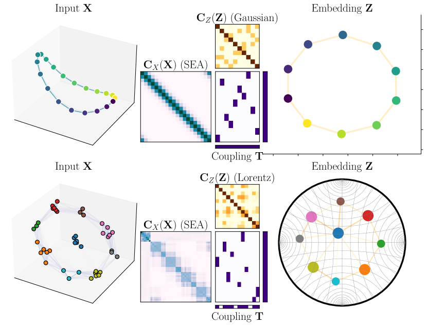
Our contributions. In this paper, we propose to bridge this gap by proposing a novel and general distributional framework that encompasses both DR and clustering as special cases. We notably cast those problems as finding a reduced distribution that minimizes the GW divergence from the original empirical data distribution. Our method proceeds by first constructing an input similarity matrix ${\bm{C}}_{X}({\bm{X}})$ that is matched with the embedding similarity ${\bm{C}}_{Z}({\bm{Z}})$ through an OT coupling matrix ${\bm{T}}$. The latter establishes correspondences between input and embedding samples. We illustrate this principle in Figure 1 where one can notice that ${\bm{C}}_{Z}({\bm{Z}})$ preserves the topology of ${\bm{C}}_{X}({\bm{X}})$ with a reduced number of nodes. The adaptivity of our model that can select an effective number of cluster $<n$, is visible in the bottom plot, where only the exact number of clusters in the original data ($9$ out of the $12$ initially proposed) is automatically recovered. Our method can operate in any embedding space, which is illustrated by projecting in either a 2D Euclidean plane or a Poincaré ball as embedding spaces.

We show that this framework is versatile and allows to recover many popular DR methods such as the kernel PCA and neighbor embedding algorithms, but also clustering algorithms such as K-means and spectral clustering. We first prove in Section 3 that DR can be formulated as a GW projection problem under some conditions on the loss and similarity functions. We then propose in Section 4 a novel formulation of data summarization as a minimal GW estimator that allows to select both the dimensionality of the embedding $d$ (DR) but also the number of Diracs $n$ (Clustering). Finally, we show in section 5 the practical interest of our approach, which regularly outperforms its competitors for various joint DR/Clustering tasks.

Notations. The $i^{th}$ entry of a vector ${\bm{v}}$ is denoted as either $v_{i}$ or $[{\bm{v}}]_{i}$. Similarly, for a matrix ${\bm{M}}$, $M_{ij}$ and $[{\bm{M}}]_{ij}$ both denote its entry $(i,j)$. $S_{N}$ is the set of permutations of ${[\![N]\!]}$. $P_{N}(\mathbb{R}^{d})$ refers to the set of discrete probability measures composed of N points of $\mathbb{R}^{d}$. $\Sigma_{N}$ stands for the probability simplex of size $N$ that is $\Sigma_{N}:=\{{\bm{h}}\in\mathbb{R}^{N}_{+}\>\text{s.t.}\>\sum_{i}h_{i}=1\}$. In all of the paper $\log({\bm{M}}),\exp({\bm{M}})$ are to be understood element-wise. For ${\bm{x}}\in\mathbb{R}^{N},\operatorname{diag}({\bm{x}})$ denotes the diagonal matrix whose elements are the $x_{i}$.

2 Background on Dimensionality Reduction and Optimal Transport

We start by reviewing the most popular DR approaches and we introduce the Gromov-Wasserstein problem.

2.1 Unified View of Dimensionality Reduction

Let ${\bm{X}}=({\bm{x}}_{1},...,{\bm{x}}_{N})^{\top}\in\mathbb{R}^{N\times p}$ be an input dataset. Dimensionality reduction focuses on constructing a low-dimensional representation or embedding ${\bm{Z}}=({\bm{z}}_{1},...,{\bm{z}}_{N})^{\top}\in\mathbb{R}^{N\times d}$, where $d<p$. The latter should preserve a prescribed geometry for the dataset encoded via a symmetric pairwise similarity matrix ${\bm{C}}_{{\bm{X}}}\in\mathbb{R}_{+}^{N\times N}$ obtained from ${\bm{X}}$. To this end, most popular DR methods optimize ${\bm{Z}}$ such that a certain pairwise similarity matrix in the output space matches ${\bm{C}}_{{\bm{X}}}$ according to some criteria. We subsequently introduce the functions

$${\bm{C}}_{X}:\mathbb{R}^{N\times p}\to\mathbb{R}^{N\times N},{\bm{C}}_{Z}:\mathbb{R}^{N\times d}\to\mathbb{R}^{N\times N}\,,$$ (1)

which define pairwise similarity matrices in the input and output space from embeddings ${\bm{X}}$ and ${\bm{Z}}$. The DR problem can be formulated quite generally as the optimization problem

$$\min_{{\bm{Z}}\in\mathbb{R}^{N\times d}}\>\sum_{(i,j)\in{[\![N]\!]}^{2}}L\big{(}[{\bm{C}}_{X}({\bm{X}})]_{ij},[{\bm{C}}_{Z}({\bm{Z}})]_{ij}\big{)}\,.$$ (DR)

where $L:\mathbb{R}\times\mathbb{R}\rightarrow\mathbb{R}$ is a loss that quantifies how similar are two points in the input space $\mathbb{R}^{p}$ compared to two points in the output space $\mathbb{R}^{d}$. Various losses are used, such as the quadratic loss $L_{2}(x,y)\coloneqq(x-y)^{2}$ or the Kullback-Leibler divergence $L_{\operatorname{KL}}(x,y)\coloneqq x\log(x/y)-x+y$. Below, we recall several popular methods that can be placed within this framework.

Spectral methods. When ${\bm{C}}_{X}({\bm{X}})$ is a positive semi-definite matrix, eq. DR recovers spectral methods by choosing the quadratic loss $L=L_{2}$ and ${\bm{C}}_{Z}({\bm{Z}})=(\langle{\bm{z}}_{i},{\bm{z}}_{j}\rangle)_{(i,j)\in{[\![N]\!]}^{2}}$ the matrix of inner products in the embedding space. Indeed, in this case, the objective value of eq. DR reduces to

$$\sum_{(i,j)\in{[\![N]\!]}^{2}}\!\!\!\!\!L_{2}([{\bm{C}}_{X}({\bm{X}})]_{ij},\langle{\bm{z}}_{i},{\bm{z}}_{j}\rangle)=\|{\bm{C}}_{X}({\bm{X}})-{\bm{Z}}{\bm{Z}}^{\top}\|^{2}_{F}\,$$

where $\|\cdot\|_{F}$ is the Frobenius norm. This problem is commonly known as kernel Principal Component Analysis (PCA) (Schölkopf et al., 1997) and an optimal solution is given by ${\bm{Z}}^{\star}=(\sqrt{\lambda_{1}}{\bm{v}}_{1},...,\sqrt{\lambda_{d}}{\bm{v}}_{d})^{\top}$ where $\lambda_{i}$ is the $i$-th largest eigenvalue of ${\bm{C}}_{X}({\bm{X}})$ with corresponding eigenvector ${\bm{v}}_{i}$ (Eckart & Young, 1936). As shown by Ham et al. (2004); Ghojogh et al. (2021), numerous dimension reduction methods can be categorized in this manner. This includes PCA when ${\bm{C}}_{X}({\bm{X}})={\bm{X}}{\bm{X}}^{\top}$ is the matrix of inner products in the input space; (classical) multidimensional scaling (Borg & Groenen, 2005), when ${\bm{C}}_{X}({\bm{X}})=-\frac{1}{2}{\bm{H}}{\bm{D}}_{\bm{X}}{\bm{H}}$ with ${\bm{D}}_{\bm{X}}$ the matrix of squared euclidean distance between the points in $\mathbb{R}^{p}$ and ${\bm{H}}={\bm{I}}_{N}-\frac{1}{N}\bm{1}_{N}\bm{1}_{N}^{\top}$ is the centering matrix; Isomap (Tenenbaum et al., 2000), with ${\bm{C}}_{X}({\bm{X}})=-\frac{1}{2}{\bm{H}}{\bm{D}}_{\bm{X}}^{(g)}{\bm{H}}$ with ${\bm{D}}_{\bm{X}}^{(g)}$ the geodesic distance matrix; Laplacian Eigenmap (Belkin & Niyogi, 2003), with ${\bm{C}}_{X}({\bm{X}})={\bm{L}}_{\bm{X}}^{\dagger}$ the pseudo-inverse of the Laplacian associated to some adjacency matrix ${\bm{W}}_{\bm{X}}$; but also Locally Linear Embedding (Roweis & Saul, 2000), and Diffusion Map (Coifman & Lafon, 2006) (for all of these examples we refer to Ghojogh et al. 2021, Table 1).

Neighbor embedding methods. An alternative group of methods relies on neighbor embedding techniques which consists in minimizing in ${\bm{Z}}$ the quantity

$$\sum_{(i,j)\in{[\![N]\!]}^{2}}L_{\operatorname{KL}}([{\bm{C}}_{X}({\bm{X}})]_{ij},[{\bm{C}}_{Z}({\bm{Z}})]_{ij})\>.$$ (NE)

Within our framework, this corresponds to eq. DR with $L=L_{\operatorname{KL}}$. The objective function of popular methods such as stochastic neighbor embedding (SNE) (Hinton & Roweis, 2002) or t-SNE (Van der Maaten & Hinton, 2008) can be derived from eq. NE with a particular choice of ${\bm{C}}_{X},{\bm{C}}_{Z}$. For instance SNE and t-SNE both consider in the input space a symmetrized version of the entropic affinity (Vladymyrov & Carreira-Perpinan, 2013; Van Assel et al., 2023). In the embedding space, ${\bm{C}}_{Z}({\bm{Z}})$ is usually constructed from a “kernel” matrix ${\bm{K}}_{\bm{Z}}$ which undergoes a scalar (Van der Maaten & Hinton, 2008), row-stochastic (Hinton & Roweis, 2002) or doubly stochastic (Lu et al., 2019; Van Assel et al., 2023) normalization. Gaussian kernel $[{\bm{K}}_{\bm{Z}}]_{ij}=\exp(-\|{\bm{z}}_{i}-{\bm{z}}_{j}\|_{2}^{2})$, or heavy-tailed Student-t kernel $[{\bm{K}}_{\bm{Z}}]_{ij}=(1+\|{\bm{z}}_{i}-{\bm{z}}_{j}\|_{2}^{2})^{-1}$, are typical choices (Van der Maaten & Hinton, 2008). We also emphasize that one can retrieve the UMAP objective (McInnes et al., 2018) from eq. DR using the binary cross-entropy loss. As described in Van Assel et al. (2022) from a probabilistic point of view, all these objectives can be derived from a common Markov random field model with various graph priors.

Remark 2.1.

The usual formulations of neighbor embedding methods rely on the loss $L(x,y)=x\log(x/y)$. However, due to the normalization, the total mass $\sum_{ij}[{\bm{C}}_{Z}({\bm{Z}})]_{ij}$ is constant (often equal to $1$) in all of the cases mentioned above. Thus the minimization in ${\bm{Z}}$ with the $L_{\operatorname{KL}}$ formulation is equivalent.

Hyperbolic geometry. The presented DR methods can also be extended to incorporate non-Euclidean geometries. Hyperbolic spaces (Chami et al., 2021; Fan et al., 2022; Guo et al., 2022; Lin et al., 2023) are of particular interest as they can capture hierarchical structures more effectively than Euclidean spaces and mitigate the curse of dimensionality by producing representations with lower distortion rates. For instance, Guo et al. (2022) adapted t-SNE by using the Poincaré distance and by changing the Student’s t-distribution with a more general hyperbolic Cauchy distribution. Notions of projection subspaces can also be adapted, e.g. Chami et al. (2021) use horospheres as one-dimensional subspaces.

2.2 Optimal Transport Across Spaces

Optimal Transport (OT) (Villani et al., 2009; Peyré et al., 2019) is a popular framework for comparing probability distributions and is at the core of our contributions. We review in this section the Gromov-Wasserstein formulation of OT aiming at comparing distributions “across spaces”.

Gromov-Wasserstein (GW). The GW framework (Mémoli, 2011; Sturm, 2012) comprises a collection of OT methods designed to compare distributions by examining the pairwise relations within each domain. For two matrices ${\bm{C}}\in\mathbb{R}^{N\times N}$, $\overline{{\bm{C}}}\in\mathbb{R}^{n\times n}$, and weights ${\bm{h}}\in\Sigma_{N},\overline{{\bm{h}}}\in\Sigma_{n}$, the GW discrepancy is defined as

$$\begin{split}&\operatorname{GW}_{L}({\bm{C}},\overline{{\bm{C}}},{\bm{h}},\overline{{\bm{h}}})\coloneqq\min_{{\bm{T}}\in{\mathcal{U}}({\bm{h}},\overline{{\bm{h}}})}E_{L}({\bm{C}},\overline{{\bm{C}}},{\bm{T}})\,,\\ &\text{where}\quad E_{L}({\bm{C}},\overline{{\bm{C}}},{\bm{T}})\coloneqq\sum_{ijkl}L(C_{ij},\overline{C}_{kl})T_{ik}T_{jl}\,,\end{split}$$ (GW)

and ${\mathcal{U}}({\bm{h}},\overline{{\bm{h}}})=\left\{{\bm{T}}\in\mathbb{R}_{+}^{N\times n}:{\bm{T}}\bm{1}_{n}={\bm{h}},{\bm{T}}^{\top}\bm{1}_{N}=\overline{{\bm{h}}}\right\}$ is the set of couplings between ${\bm{h}}$ and $\overline{{\bm{h}}}$. In this formulation, both pairs $({\bm{C}},{\bm{h}})$ and $(\overline{{\bm{C}}},\overline{{\bm{h}}})$ can be interpreted as graphs with corresponding connectivity matrices ${\bm{C}},\overline{\bm{C}}$, and where nodes are weighted by histograms ${\bm{h}},\overline{\bm{h}}$. Equation GW is thus a quadratic problem (in ${\bm{T}}$) which consists in finding a soft-assignment matrix ${\bm{T}}$ that aligns the nodes of the two graphs in a way that preserves their pairwise connectivities.

From a distributional perspective, GW can also be viewed as a distance between distributions that do not belong to the same metric space. For two discrete probability distributions $\mu_{X}=\sum_{i=1}^{N}[{\bm{h}}_{X}]_{i}\delta_{{\bm{x}}_{i}}\in{\mathcal{P}}_{N}(\mathbb{R}^{p}),\mu_{Z}=\sum_{i=1}^{n}[{\bm{h}}_{Z}]_{i}\delta_{{\bm{z}}_{i}}\in{\mathcal{P}}_{n}(\mathbb{R}^{d})$ and pairwise similarity matrices ${\bm{C}}_{X}({\bm{X}})$ and ${\bm{C}}_{Z}({\bm{Z}})$ associated with the supports ${\bm{X}}=({\bm{x}}_{1},\cdots,{\bm{x}}_{n})^{\top}$ and ${\bm{Z}}=({\bm{z}}_{1},\cdots,{\bm{z}}_{n})^{\top}$, the quantity $\operatorname{GW}_{L}({\bm{C}}_{X}({\bm{X}}),{\bm{C}}_{Z}({\bm{Z}}),{\bm{h}}_{X},{\bm{h}}_{Z})$ is a measure of dissimilarity or discrepancy between $\mu_{X},\mu_{Z}$. Specifically, when $L=L_{2}$, and ${\bm{C}}_{X}({\bm{X}}),{\bm{C}}_{Z}({\bm{Z}})$ are pairwise distance matrices, GW defines a proper distance between $\mu_{X}$ and $\mu_{Z}$ with respect to measure preserving isometries (Mémoli, 2011).

Due to its versatile properties, notably in comparing distributions over different domains, the GW problem has found many applications in machine learning, e.g., for 3D meshes alignment (Solomon et al., 2016; Ezuz et al., 2017), NLP (Alvarez-Melis & Jaakkola, 2018), (co-)clustering (Peyré et al., 2016; Redko et al., 2020), single-cell analysis (Demetci et al., 2020), neuroimaging (Thual et al., 2022), graph representation learning (Xu, 2020; Vincent-Cuaz et al., 2021; Liu et al., 2022b; Vincent-Cuaz et al., 2022b; Zeng et al., 2023) and partitioning (Xu et al., 2019; Chowdhury & Needham, 2021).

In this work, we leverage the GW discrepancy to extend classical DR approaches, framing them as the projection of a distribution onto a space of lower dimensionality.

3 Dimensionality Reduction as OT

In this section, we present the strong connections between the classical eq. DR and the GW problem.

Gromov-Monge interpretation of DR. As suggested by eq. DR, dimension reduction seeks to find embeddings ${\bm{Z}}$ so that the similarity between the $(i,j)$ samples of the input data is as close as possible to the similarity between the $(i,j)$ samples of the embeddings. Under reasonable assumptions about ${\bm{C}}_{Z}$, this also amounts to identifying the embedding ${\bm{Z}}$ and the best permutation that realigns the two similarity matrices. Recall that the function ${\bm{C}}_{Z}$ is equivariant by permutation, if, for any $N\times N$ permutation matrix ${\bm{P}}$ and any ${\bm{Z}}$, ${\bm{C}}_{Z}({\bm{P}}{\bm{Z}})={\bm{P}}{\bm{C}}_{Z}({\bm{Z}}){\bm{P}}^{\top}$ (Bronstein et al., 2021). This type of assumption is natural for ${\bm{C}}_{Z}$: if we rearrange the order of samples (i.e. , the rows of ${\bm{Z}}$), we expect the similarity matrix between the samples to undergo the same rearrangement.

Lemma 3.1.

Let ${\bm{C}}_{Z}$ be a permutation equivariant function and $L$ any loss. The minimum eq. DR is equal to

$$\min_{{\bm{Z}}\in\mathbb{R}^{N\times d}}\min_{\sigma\in S_{N}}\sum_{ij}L([{\bm{C}}_{X}({\bm{X}})]_{ij},[{\bm{C}}_{Z}({\bm{Z}})]_{\sigma(i)\sigma(j)})\>.$$ (2)

Also, any sol. ${\bm{Z}}$ of eq. DR is such that $({\bm{Z}},\operatorname{id})$ is sol. of eq. 2 and conversely any $({\bm{Z}},\sigma)$ sol. of eq. 2 is such that ${\bm{Z}}$ is a sol of eq. DR up to $\sigma$.

See proof in Section A.1. The correspondence established between eq. DR and eq. 2 unveils a quadratic problem similar to GW. Specifically, eq. 2 relates to the Gromov-Monge problem (Mémoli & Needham, 2018) which seeks to identify, by solving a quadratic assignment problem (Cela, 2013), the permutation $\sigma$ that best aligns two similarity matrices. Lemma 3.1 therefore shows that the best permutation is the identity when we also optimize the embedding ${\bm{Z}}$. We can delve deeper into these comparisons and demonstrate that the general formulation of dimension reduction is also equivalent to minimizing the Gromov-Wasserstein objective, which serves as a relaxation of the Gromov-Monge problem (Mémoli & Needham, 2022).

DR as GW Minimization. We suppose that the distributions have the same number of points ($N=n$) and uniform weights (${\bm{h}}_{Z}={\bm{h}}_{X}=\frac{1}{N}\bm{1}_{N}$). We recall that a matrix ${\bm{C}}\in\mathbb{R}^{N\times N}$ is conditionally positive definite (CPD), resp. conditionally negative definite (CND), if it is symmetric and $\forall{\bm{x}}\in\mathbb{R}^{N},{\bm{x}}^{\top}\mathbf{1}_{N}=0\text{ s.t. }{\bm{x}}^{\top}{\bm{C}}{\bm{x}}\geq 0$, resp. $\leq 0$.

We thus have the following theorem that extends Lemma 3.1 to the GW problem (proof can be found in Section A.2).

Theorem 3.2.

The minimum eq. DR is equal to $\min_{{\bm{Z}}}\operatorname{GW}_{L}({\bm{C}}_{X}({\bm{X}}),{\bm{C}}_{Z}({\bm{Z}}),\frac{1}{N}\bm{1}_{N},\frac{1}{N}\bm{1}_{N})$ in the following settings:

1. (spectral methods) ${\bm{C}}_{X}({\bm{X}})$ is any matrix, $L=L_{2}$ and ${\bm{C}}_{Z}({\bm{Z}})={\bm{Z}}{\bm{Z}}^{\top}$.

2. (neighbor embedding methods) $\operatorname{Im}({\bm{C}}_{X})\subseteq\mathbb{R}_{>0}^{N\times N}$, $L=L_{\operatorname{KL}}$, the matrix ${\bm{C}}_{X}({\bm{X}})$ is CPD and, for any ${\bm{Z}}$,

   $${\bm{C}}_{Z}({\bm{Z}})=\operatorname{diag}(\bm{\alpha}_{\bm{Z}}){\bm{K}}_{\bm{Z}}\operatorname{diag}(\bm{\beta}_{\bm{Z}})\,,$$ (3)

   where $\bm{\alpha}_{\bm{Z}},\bm{\beta}_{\bm{Z}}\in\mathbb{R}^{N}_{>0}$ and ${\bm{K}}_{\bm{Z}}\in\mathbb{R}^{N\times N}_{>0}$ is such that $\log({\bm{K}}_{\bm{Z}})$ is CPD.

Remarkably, this result shows that all spectral DR methods can be seen as OT problems in disguise, as they all equivalently minimize a GW problem. The second point of the theorem also provides some insights into this equivalence in the case of neighbor embedding methods. For instance, the Gaussian kernel ${\bm{K}}_{\bm{Z}}$, used extensively in DR, satisfies the hypothesis as $\log({\bm{K}}_{\bm{Z}})=(-\|{\bm{z}}_{i}-{\bm{z}}_{j}\|_{2}^{2})_{ij}$ is CPD (see e.g. Maron & Lipman 2018). The terms $\bm{\alpha}_{\bm{Z}},\bm{\beta}_{\bm{Z}}$ also allow for considering all the usual normalizations of ${\bm{K}}_{\bm{Z}}$: by a scalar so as to have $\sum_{ij}[{\bm{C}}_{Z}({\bm{Z}})]_{ij}=1$, but also any row-stochastic or doubly stochastic normalization (with the Sinkhorn-Knopp algorithm Sinkhorn & Knopp 1967).

Matrices satisfying $\log({\bm{K}}_{\bm{Z}})$ being CPD are well-studied in the literature and are known as infinitely divisible matrices (Bhatia, 2006). It is noteworthy that the t-Student kernel does not fall into this category. Moreover, in the aforementioned neighbor embedding methods, the matrix ${\bm{C}}_{X}({\bm{X}})$ is generally not CPD. The intriguing question of generalizing this result with weaker assumptions on ${\bm{C}}_{Z}$ and ${\bm{C}}_{X}$ remains open for future research. Interestingly, we have observed in the numerical experiments performed in Section 5 that the symmetric entropic affinity of Van Assel et al. (2023) was systematically CPD.

Remark 3.3.

In Corollary A.3 of the appendix we also provide other sufficient conditions for neighbor embedding methods with the cross-entropy loss $L(x,y)=x\log(x/y)$. They rely on specific structures for ${\bm{C}}_{Z}$ but do not impose any assumptions on ${\bm{C}}_{X}$. Additionally, in Section A.3, we provide a necessary condition based on a bilinear relaxation of the GW problem. Although its applicability is limited due to challenges in proving it in full generality, it requires minimal assumptions on ${\bm{C}}_{X},{\bm{C}}_{Z}$ and $L$.

In essence, both Lemma 3.1 and Theorem 3.2 indicate that dimensionality reduction can be reframed from a distributional perspective, with the search for an empirical distribution that aligns with the data distribution in the sense of optimal transport, through the lens of GW. In other words, DR is informally solving $\min_{{\bm{z}}_{1},\cdots,{\bm{z}}_{N}}\operatorname{GW}(\frac{1}{n}\sum_{i=1}^{N}\delta_{{\bm{x}}_{i}},\frac{1}{n}\sum_{i=1}^{N}\delta_{{\bm{z}}_{i}})$.

4 Distributional Reduction

The previous interpretation is significant because it allows for two generalizations. Firstly, beyond solely determining the positions ${\bm{z}}_{i}$ of Diracs (as in classical DR) we can now optimize the mass of the distribution $\mu_{Z}$. This is interpreted as finding the relative importance of each point in the embedding ${\bm{Z}}$. More importantly, due to the flexibility of GW, we can also seek a distribution in the embedding with a smaller number of points $n<N$. This will result in both reducing the dimension and clustering the points in the embedding space through the optimal coupling. Informally, our Distributional Reduction (DistR) framework aims at solving $\min_{\mu_{Z}\in{\mathcal{P}}_{n}(\mathbb{R}^{d})}\operatorname{GW}(\frac{1}{n}\sum_{i=1}^{N}\delta_{{\bm{x}}_{i}},\mu_{Z})$.

4.1 Distributional Reduction Problem

Precisely, the optimization problem that we tackle in this paper can be formulated as follows

$$\min_{\begin{smallmatrix}{\bm{Z}}\in\mathbb{R}^{n\times d}\\ {\bm{h}}_{Z}\in\Sigma_{n}\end{smallmatrix}}\operatorname{GW}_{L}({\bm{C}}_{X}({\bm{X}}),{\bm{C}}_{Z}({\bm{Z}}),{\bm{h}}_{X},{\bm{h}}_{Z})$$ (DistR)

This problem comes down to learning the closest graph $({\bm{C}}_{Z}({\bm{Z}}),{\bm{h}}_{Z})$ parametrized by ${\bm{Z}}$ from $({\bm{C}}_{X}({\bm{X}}),{\bm{h}}_{X})$ in the GW sense. When $n<N$, the embeddings $({\bm{z}}_{1},\cdots,{\bm{z}}_{n})$ then act as low-dimensional prototypical examples of input samples, whose learned relative importance ${\bm{h}}_{Z}$ accommodates clusters of varying proportions in the input data ${\bm{X}}$ (see Figure 1). We refer to them as prototypes. The weight vector ${\bm{h}}_{X}$ is typically assumed to be uniform, that is ${\bm{h}}_{X}=\frac{1}{N}\bm{1}_{N}$, in the absence of prior knowledge. As discussed in Section 3, traditional DR amounts to setting $n=N,{\bm{h}}_{Z}=\frac{1}{N}\bm{1}_{N}$.

Clustering with DistR. One notable aspect of our model is its capability to simultaneously perform dimensionality reduction and clustering. Indeed, the optimal coupling ${\bm{T}}\in[0,1]^{N\times n}$ of problem eq. DistR is, by construction, a soft-assignment matrix from the input data to the embeddings. It allows each point ${\bm{x}}_{i}$ to be linked to one or more prototypes ${\bm{z}}_{j}$ (clusters). In Section 4.2 we explore conditions where these soft assignments transform into hard ones, such that each point is therefore linked to a unique prototype/cluster.

Figure 2: GW projections of a single-cell genomics dataset (Chen et al., 2019) on regular grids with increasing resolutions, respectively encoded as $C_{X}({\bm{X}})={\bm{X}}{\bm{X}}^{\top}$ and $C_{Z}({\bm{Z}})={\bm{Z}}{\bm{Z}}^{\top}$. Pixels on cropped grids are colored by interpolating samples’ colors according to the transport plan and their intensity is proportional to their mass.

A semi-relaxed objective.

For a given embedding ${\bm{Z}}$ and $L=L_{2}$, it is known that minimizing in ${\bm{h}}_{Z}$ the DistR objective is equivalent to a problem that is computationally simpler than the usual GW one, namely the semi-relaxed GW divergence $\operatorname{srGW}_{L}$ (Vincent-Cuaz et al., 2022a):

$$\min_{{\bm{T}}\in{\mathcal{U}}_{n}({\bm{h}}_{X})}E_{L}({\bm{C}}_{X}({\bm{X}}),{\bm{C}}_{Z}({\bm{Z}}),{\bm{T}})\>,$$ (srGW)

where ${\mathcal{U}}_{n}({\bm{h}}_{X}):=\left\{{\bm{T}}\in\mathbb{R}_{+}^{N\times n}:{\bm{T}}\bm{1}_{n}={\bm{h}}_{X}\right\}$. To efficiently address eq. DistR, we first observe that this equivalence holds for any inner divergence $L$ with a straightforward adaptation of the proof in Vincent-Cuaz et al. (2022a). Additionally, we prove that $\operatorname{srGW}_{L}$ remains a divergence as soon as $L$ is itself a divergence. Consequently, $\operatorname{srGW}_{L}$ vanishes iff both measures are isomorphic in a weak sense (Chowdhury & Mémoli, 2019). We emphasize that taking a proper divergence $L$ is important (and basic assumptions on ${\bm{X}}$), as it avoids some trivial solutions as detailed in Appendix B.

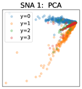
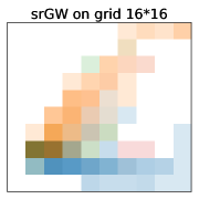
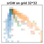
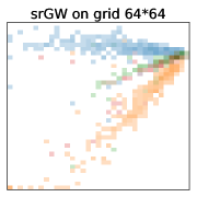
Interestingly, srGW projections, i.e. optimizing only the weights ${\bm{h}}_{Z}$ over simple fixed supports ${\bm{Z}}$, have already remarkable representational capability. We illustrate this in Figure 2, by considering projections of a real-world dataset over 2D grids of increasing resolutions. Setting ${\bm{C}}_{X}({\bm{X}})={\bm{X}}{\bm{X}}^{\top}$ and ${\bm{C}}_{Z}({\bm{X}})={\bm{Z}}{\bm{Z}}^{\top}$, we can see that those projections recover faithful coarsened representations of the embeddings learned using PCA. DistR aims to exploit the full potential of this divergence by learning a few optimal prototypes that best represent the dataset.

4.2 Clustering Properties

In addition to the connections established between DistR and DR methods in Section 3, we elaborate now on the links between DistR and clustering methods. In what follows, we call a coupling ${\bm{T}}\in[0,1]^{N\times n}$ with a single non-null element per row a membership matrix. When the coupling is a membership matrix each data point is associated with a single prototype thus achieving a hard clustering of the input samples.

We will see that a link can be drawn with kernel K-means using the analogy of GW barycenters. More precisely the srGW barycenter (Vincent-Cuaz et al., 2022a) seeks for a closest target graph $(\overline{{\bm{C}}},\overline{{\bm{h}}})$ from $({\bm{C}}_{X},{\bm{h}}_{X})$ by solving

$$\min_{\overline{{\bm{C}}}\in\mathbb{R}^{n\times n}}\min_{{\bm{T}}\in\mathcal{U}_{n}({\bm{h}}_{X})}E_{L}({\bm{C}}_{X}({\bm{X}}),\overline{{\bm{C}}},{\bm{T}})\>.$$ (srGWB)

We emphasize that the only (important) difference between eq. srGWB and eq. DistR is that there is no constraint imposed on $\overline{{\bm{C}}}$ in srGWB. In contrast, eq. DistR looks for minimizing over $\overline{{\bm{C}}}\in\{{\bm{C}}_{Z}({\bm{Z}}):{\bm{Z}}\in\mathbb{R}^{N\times d}\}$. For instance, choosing ${\bm{C}}_{Z}({\bm{Z}})={\bm{Z}}{\bm{Z}}^{\top}$ in eq. DistR is equivalent to enforcing $\operatorname{rank}(\overline{{\bm{C}}})\leq d$ in eq. srGWB.

Figure 3: Examples of 2-dimensional embeddings produced by DistR using the SEA similarity for ${\bm{C}}_{X}$ and the Student’s kernel for ${\bm{C}}_{Z}$. The latter computed in $\mathbb{R}^{2}$ for the first three datasets and the Poincaré ball for the last one. Displayed images are medoids for each cluster i.e. $\operatorname*{arg\,max}_{i}[{\bm{C}}_{X}({\bm{X}}){\bm{T}}_{:,k}]_{i}$ for cluster $k$. The area of image $k$ is proportional to $[{\bm{h}}_{Z}]_{k}$.

We establish below that srGWB is of particular interest for clustering. The motivation for this arises from the findings of Chen et al. (2023), which demonstrate that when ${\bm{C}}_{X}({\bm{X}})$ is positive semi-definite and ${\bm{T}}$ is constrained to belong to the set of membership matrices (as opposed to couplings in ${\mathcal{U}}_{n}({\bm{h}})$), eq. srGWB is equivalent to a kernel K-means whose samples are weighted by ${\bm{h}}_{X}$ (Dhillon et al., 2004, 2007). These additional constraints are in fact unnecessary since we show below that the original srGWB problem admits membership matrices as the optimal coupling for a broader class of ${\bm{C}}_{X}({\bm{X}})$ input matrices (see proofs in appendix C).

Theorem 4.1.

Let ${\bm{h}}_{X}\in\Sigma_{N}$ and $L=L_{2}$. Suppose that for any ${\bm{X}}\in\mathbb{R}^{N\times p}$ the matrix ${\bm{C}}_{X}({\bm{X}})$ is CPD or CND. Then the problem eq. srGWB admits a membership matrix as optimal coupling, i.e. , there is a minimizer of ${\bm{T}}\in\mathcal{U}_{n}({\bm{h}}_{X})\to\min_{\overline{{\bm{C}}}\in\mathbb{R}^{n\times n}}E_{L}({\bm{C}}_{X}({\bm{X}}),\overline{{\bm{C}}},{\bm{T}})$ with only one non-zero value per row.

Theorem 4.1 and relations proven in Chen et al. (2023) provide that eq. srGWB is equivalent to the aforementioned kernel K-means when ${\bm{C}}_{X}({\bm{X}})$ is positive semi-definite. Moreover, as the (hard) clustering property holds for more generic types of matrices, namely CPD and CND, srGWB stands out as a fully-fledged clustering method. Although these results do not apply directly to DistR, we argue that they further legitimize the use of GW projections for clustering. Interestingly, we also observe in practice that the couplings obtained by DistR are always membership matrices, regardless of ${\bm{C}}_{Z}$. Further research will be carried out to better understand this phenomenon.

4.3 Computation

DistR is a non-convex problem that we propose to tackle using a Block Coordinate Descent algorithm (BCD, Tseng 2001) guaranteed to converge to local optimum (Grippo & Sciandrone, 2000; Lyu & Li, 2023). The BCD alternates between the two following steps. First, we optimize in ${\bm{Z}}$ for a fixed transport plan using gradient descent with adaptive learning rates (Kingma & Ba, 2014). Then we solve for a srGW problem given ${\bm{Z}}$. To this end, we benchmarked both the Conditional Gradient and Mirror Descent algorithms proposed in Vincent-Cuaz et al. (2022a), extended to support losses $L_{2}$ and $L_{\operatorname{KL}}$.

Following Proposition 1 in (Peyré et al., 2016), a vanilla implementation leads to $\mathcal{O}(nN^{2}+n^{2}N)$ operations to compute the loss or its gradient. In many DR methods, ${\bm{C}}_{X}({\bm{X}})$ or ${\bm{C}}_{Z}({\bm{Z}})$, or their transformations within the loss $L$, admit explicit low-rank factorizations. Including e.g. matrices involved in spectral methods and other similarity matrices derived from squared Euclidean distance matrices (Scetbon et al., 2022). In these settings, we exploit these factorizations to reduce the computational complexity of our solvers down to $\mathcal{O}(Nn(p+d)+(N+m)pd+n^{2})$ when $L=L_{2}$, and $O(Nnd+n^{2}d)$ when $L=L_{\operatorname{KL}}$. We refer the reader interested in these algorithmic details to Appendix D.

4.4 Related Work

The closest to our work is the CO-Optimal-Transport (COOT) clustering approach proposed in (Redko et al., 2020) that estimates simultaneously a clustering of samples and features through the CO-Optimal Transport problem,

$$\min_{\begin{subarray}{c}{\bm{T}}_{1}\in{\mathcal{U}}({\bm{h}}_{1},\overline{{\bm{h}}}_{1})\\ {\bm{T}}_{2}\in{\mathcal{U}}({\bm{h}}_{2},\overline{{\bm{h}}}_{2})\end{subarray}}\>\sum_{ijkl}(X_{ik}-Z_{jl})^{2}[{\bm{T}}_{1}]_{ij}[{\bm{T}}_{2}]_{kl}\,,$$ (COOT)

where ${\bm{h}}_{1}\in\Sigma_{N}$, $\overline{{\bm{h}}}_{1}\in\Sigma_{n}$, ${\bm{h}}_{2}\in\Sigma_{p}$ and $\overline{{\bm{h}}}_{2}\in\Sigma_{d}$. We emphasize that COOT-clustering, which consists in optimizing the COOT objective above w.r.t. ${\bm{Z}}$, is a linear DR model as the reduction is done with the map ${\bm{T}}_{2}$. In contrast, DistR leverages the more expressive non-linear similarity functions of existing DR methods. Other joint DR-clustering approaches, such as (Liu et al., 2022a), involve modeling latent variables by a mixture of distributions. In comparison, our framework is more versatile, as it can easily adapt to any $(L,{\bm{C}}_{X},{\bm{C}}_{Z})$ of existing DR methods (Section 2.1).

	methods	${\bm{C}}_{X}/{\bm{C}}_{Z}$	MNIST	FMNIST	COIL	SNA1	SNA2	ZEI1	ZEI2	PBMC
$d=10$	DistR (ours)	$\langle,\rangle_{\mathbb{R}^{p}}$ / $\langle,\rangle_{\mathbb{R}^{d}}$	76.9 (0.4)	74.0 (0.6)	77.4 (0.7)	75.6 (0.0)	86.6 (2.9)	76.5 (1.0)	49.1 (1.9)	86.3 (0.5)
	$\text{DistR}_{\varepsilon}$ (ours)	-	76.5 (0.0)	74.5 (0.0)	78.5 (0.0)	68.9 (0.2)	78.9 (1.3)	79.8 (0.2)	52.7 (0.2)	85.1 (0.0)
	DR$\to$C	-	73.9 (1.7)	63.9 (0.0)	70.6 (3.3)	77.3 (2.5)	66.9(14.3)	73.6 (0.8)	26.9 (7.9)	76.9 (1.2)
	C$\to$DR	-	76.5 (0.0)	74.3 (0.0)	62.3 (0.0)	68.3 (0.2)	86.0 (0.3)	79.6 (0.1)	52.5 (0.1)	86.0 (0.0)
	COOT	NA	32.8 (2.5)	28.2 (6.0)	47.9 (1.0)	49.3 (6.8)	76.6 (6.5)	81.0 (2.4)	30.0 (1.6)	34.5 (1.3)
$d=2$	DistR (ours)	SEA / St.	77.5 (0.8)	76.8 (0.5)	83.3 (0.7)	80.2 (1.9)	88.5 (0.0)	81.0 (0.6)	47.6 (1.1)	82.5 (1.2)
	$\text{DistR}_{\varepsilon}$ (ours)	-	77.9 (0.2)	75.6 (0.6)	83.9 (0.5)	80.4 (1.8)	90.7 (0.1)	79.9 (0.2)	48.2 (0.6)	86.4 (0.2)
	DR$\to$C	-	74.8 (0.9)	75.7 (0.5)	80.3 (0.5)	77.2 (0.4)	89.3 (0.1)	79.0 (0.5)	47.4 (2.7)	82.0 (1.7)
	C$\to$DR	-	76.2 (0.6)	75.0 (0.3)	81.6 (0.3)	77.6 (0.5)	89.8 (0.1)	78.8 (0.7)	45.8 (0.9)	88.4 (0.5)
	COOT	NA	26.1 (5.7)	24.9 (1.5)	42.5 (2.5)	32.6 (5.1)	56.8 (4.0)	78.2 (0.7)	25.2 (0.6)	28.9 (3.2)
$d=2$	DistR (ours)	SEA / H-St.	75.0 (0.0)	75.3 (0.6)	70.2 (0.8)	75.4 (0.8)	88.9 (1.8)	77.4 (3.1)	41.6 (1.7)	73.2 (1.6)
	$\text{DistR}_{\varepsilon}$ (ours)	-	66.9 (0.5)	66.4 (0.3)	69.6 (0.9)	81.3 (5.1)	78.6 (1.0)	73.6 (1.8)	38.6 (0.7)	72.9 (2.3)
	DR$\to$C	-	58.4 (4.6)	59.7 (9.7)	47.4 (1.5)	51.8 (5.9)	58.1 (9.9)	80.6 (5.2)	41.5 (2.4)	67.4 (7.2)
	C$\to$DR	-	67.1 (1.8)	66.3 (0.5)	71.1 (1.1)	80.8 (3.9)	75.0(0.0)	71.2 (0.9)	37.5 (0.4)	67.6 (0.4)

Table 1: Average $\overline{\mathcal{SH}}$ scores (with standard deviation) for the main experiment (Section 5). The reported results are averaged on 5 different random seeds. The best result is in bold, second best is underlined. DistR refers to our solution relying on the conditional gradient to update ${\bm{T}}$ while $\text{DistR}_{\varepsilon}$ relies on $\operatorname{KL}$ mirror descent (details in Section 4.3 and Appendix D). Finally, St. refers to the Student’s kernel and H-St. is its equivalent in the hyperbolic context.

5 Numerical Experiments

In this section, we demonstrate the relevance of our approach for joint clustering and dimensionality reduction.

Datasets. We experiment with popular labeled image datasets: COIL-20 (Nene et al., 1996), MNIST and fashion-MNIST (Xiao et al., 2017) as well as the following single-cell genomics datasets: PBMC 3k (Wolf et al., 2018), SNAREseq chromatin and gene expression (Chen et al., 2019) and the scRNA-seq dataset from Zeisel et al. (2015) with two hierarchical levels of label. Dataset sizes and pre-processing steps are detailed in appendix E.

Benchmarked methods. Let us recall that any DR method presented in Section 2.1 is fully characterized by a triplet $(L,{\bm{C}}_{X},{\bm{C}}_{Z})$ of loss and pairwise similarity functions. Given $(L,{\bm{C}}_{X},{\bm{C}}_{Z})$, we compare our DistR model against sequential approaches of DR and clustering. Namely DR then clustering (DR$\to$C) and Clustering then DR (C$\to$DR) using the DR method associated with the same triplet. DR$\to$C representations are constructed by first running the DR method (Section 2.1) associated with $(L,{\bm{C}}_{X},{\bm{C}}_{Z})$ thus obtaining an intermediate representation $\widetilde{{\bm{Z}}}\in\mathbb{R}^{N\times p}$. Then, spectral clustering (Von Luxburg, 2007) on the similarity matrix ${\bm{C}}_{Z}(\widetilde{{\bm{Z}}})$ is performed to compute a cluster assignment matrix $\widetilde{{\bm{T}}}\in\mathbb{R}^{N\times n}$. The final reduced representation in $\mathbb{R}^{n\times p}$ is the average of each point per cluster, i.e. the collection of the centroids, which is formally $\operatorname{diag}(\tilde{{\bm{h}}})^{-1}\widetilde{{\bm{T}}}^{\top}\widetilde{{\bm{Z}}}\in\mathbb{R}^{n\times p}$ where $\tilde{{\bm{h}}}=\widetilde{{\bm{T}}}^{\top}\bm{1}_{N}$. For C$\to$DR, a cluster assignment matrix $\widehat{{\bm{T}}}\in\mathbb{R}^{N\times n}$ is first computed using spectral clustering on ${\bm{C}}_{X}({\bm{X}})$. Then, the cluster centroid $\operatorname{diag}(\hat{{\bm{h}}})^{-1}\widehat{{\bm{T}}}^{\top}{\bm{X}}$, where $\hat{{\bm{h}}}=\widehat{{\bm{T}}}^{\top}\bm{1}_{N}$, is passed as input to the DR method associated with $(L,{\bm{C}}_{X},{\bm{C}}_{Z})$. Finally, we compare against the COOT-clustering model which enables to perform clustering and DR jointly but with many limitations compared to DistR as discussed in Section 4.4.

Implementation details. Throughout, the spectral clustering implementation of scikit-learn (Pedregosa et al., 2011) is used to perform either the clustering steps or the initialization of transport plans. For all methods, ${\bm{Z}}$ is initialized from i.i.d. sampling of the standard gaussian distribution $\mathcal{N}(0,1)$ (or an equivalent Wrapped Normal distribution in Hyperbolic spaces (Nagano et al., 2019)), and further optimized using PyTorch’s automatic differentiation (Paszke et al., 2017) with Adam optimizer (Kingma & Ba, 2014), or with RAdam in hyperbolic settings (Bécigneul & Ganea, 2018). OT-based solvers are built upon the POT (Flamary et al., 2021) library. and computations in Hyperbolic spaces with Geoopt (Kochurov et al., 2020). For the Hyperbolic space, all the computations were conducted in the Lorentz model (Nickel & Kiela, 2018), which is less prone to numerical errors. As such, we used the associated distance function to form ${\bm{C}}_{Z}$. After optimization, results are projected back to the Poincaré ball for visualization purpose. In this hyperbolic context, we adopted the formulation and the default hyperparameters of Guo et al. (2022) which generalize Student’s t-distributios by Hyperbolic Cauchy distributions (denoted as H-St in the results Table 1). Evaluation metric. We aim to evaluate both the DR and clustering abilities of our method DistR. For clustering evaluation, we use the homogeneity_score of Torchmetrics (Rosenberg & Hirschberg, 2007; Detlefsen et al., 2022) and denoted by ${\mathcal{H}}$. Relying on known class labels ${\bm{y}}$, this score ranging from $0$ to $1$ quantifies the extent to which each prototype ${\bm{z}}_{k}$ receives mass through ${\bm{T}}$ from points within the same class. To assess DR performance, we make use of the silhouette score (Rousseeuw, 1987) ranging from $-1$ to $1$. This score is computed by first associating with each prototype ${\bm{z}}_{k}$ a label defined by the $y$ maximizing $\sum_{i\in{[\![N]\!]}}T_{ik}\bm{1}_{y_{i}=y}$ where $y_{i}$ is the class label of the input data point ${\bm{x}}_{i}$. Then it evaluates whether the relative position of prototypes, quantified via the appropriate metric depending on the embedding space, is aligned with the label they are assigned to. To compute the final silhouette, we slightly adapt the usual criterion to take into account the relative importance of each ${\bm{z}}_{k}$ given by the amount of mass it receives, that is $\sum_{i\in{[\![N]\!]}}T_{ik}$. More details can be found in Appendix E. We use the notation $\mathcal{S}$ for this score. To best quantify the trade-off between clustering and DR, our final general criterion is defined as the average of the homogeneity and silhouette score, where the latter is rescaled and shifted such that it ranges from $0$ to $1$, i.e.

$$\overline{\mathcal{SH}}=\frac{1}{2}\left(\frac{\mathcal{S}+1}{2}+\mathcal{H}\right)\,.$$ (Score)

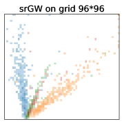
Setting and discussion. We experiment using both spectral and neighbor embedding methods (NE) for $(L,{\bm{C}}_{X},{\bm{C}}_{Z})$. For spectral, we consider the usual PCA setting which amounts to ${\bm{C}}_{X}({\bm{X}})={\bm{X}}{\bm{X}}^{\top}$ and ${\bm{C}}_{Z}({\bm{Z}})={\bm{Z}}{\bm{Z}}^{\top}$ choosing $d=10$ as embedding dimension. Regarding NE, we rely on the Symmetric Entropic Affinity (SEA) from (Van Assel et al., 2023) for ${\bm{C}}_{X}$ and the scalar-normalized student similarity for ${\bm{C}}_{Z}$ (Van der Maaten & Hinton, 2008) in dimension $d=2$. The SEA similarity enables controlling both mass and entropy making it robust to varying noise levels and depends on the perplexity hyperparameter $\xi$ which determines the considered scale of dependency. For each configuration, we select the parameter $\xi$ across the set $\{20,50,100,150,200,250\}$, while the number of output samples $n$ is validated in a set of $10$ values, starting at the number of classes in the data and incrementing in steps of $20$. For the computation of ${\bm{T}}$ in DistR (see Section 4.3), we benchmark our Conditional Gradient solver, and the Mirror Descent algorithm whose parameter $\varepsilon$ is validated in the set $\{0.1,1,10\}$. $\overline{\mathcal{SH}}$ scores are displayed in Table 1. We also provide, in Appendix E, the corresponding separated scores $\mathcal{S}$ and $\mathcal{H}$. They show the superiority of DistR for $80\%$ of the considered configurations. Therefore, our approach effectively achieves the ideal equilibrium between homogeneity and preservation of the structure of the prototypes. For a qualitative illustration, we display some embeddings produced by our method in Figure 3.

6 Conclusion

After making a connection between the GW problem and popular clustering and DR algorithms, we proposed a unifying framework denoted as DistR, enabling to jointly reduce the feature and sample sizes of an input dataset. We believe that the versatility of the GW framework will enable new extensions in unsupervised learning. For instance, the formalism associated with (semi-relaxed) GW barycenters naturally enables considering multiple inputs, potentially unaligned and of different sizes. Hence our approach can be useful to address challenges related to the multi-view dimensionality reduction and clustering problems. Other promising directions involve better capturing multiple dependency scales in the input data by hierarchically adapting the resolution of the embedding similarity graph.

Appendix A Proof of results in Section 3

A.1 Proof of Lemma 3.1

We recall the result. See 3.1

Proof.

By suboptimality of $\sigma=\operatorname{id}$ we clearly have $\min_{{\bm{Z}}\in\mathbb{R}^{N\times d}}\min_{\sigma\in S_{N}}\sum_{ij}L([{\bm{C}}_{X}({\bm{X}})]_{ij},[{\bm{C}}_{Z}({\bm{Z}})]_{\sigma(i)\sigma(j)})\leq\min_{{\bm{Z}}\in\mathbb{R}^{N\times d}}\sum_{ij}L([{\bm{C}}_{X}({\bm{X}})]_{ij},[{\bm{C}}_{Z}({\bm{Z}})]_{ij})$. For the other direction, take an optimal solution $({\bm{Z}},\sigma)$ of eq. 2. Using the permutation equivariance of ${\bm{C}}_{Z}$, $[{\bm{C}}_{Z}({\bm{Z}})]_{\sigma(i)\sigma(j)}=[{\bm{P}}{\bm{C}}_{Z}({\bm{Z}}){\bm{P}}^{\top}]_{ij}=[{\bm{C}}_{Z}({\bm{P}}{\bm{Z}})]_{ij}$ for some permutation matrix ${\bm{P}}$. But ${\bm{P}}{\bm{Z}}$ is admissible for problem eq. DR. Hence $\min_{{\bm{Z}}\in\mathbb{R}^{N\times d}}\min_{\sigma\in S_{N}}\sum_{ij}L([{\bm{C}}_{X}({\bm{X}})]_{ij},[{\bm{C}}_{Z}({\bm{Z}})]_{\sigma(i)\sigma(j)})\geq\min_{{\bm{Z}}\in\mathbb{R}^{N\times d}}\sum_{ij}L([{\bm{C}}_{X}({\bm{X}})]_{ij},[{\bm{C}}_{Z}({\bm{Z}})]_{ij})$. ∎

A.2 Proof of Theorem 3.2

In the following $\operatorname{DS}$ is the space of $N\times N$ doubly stochastic matrices. We begin by proving the first point of Theorem 3.2. We will rely on the simple, but useful, result below

Proposition A.1.

Let $\Omega\subseteq\mathbb{R}$ and $\operatorname{Im}({\bm{C}}_{X})\subseteq\Omega^{N\times N}$. Suppose that $L(a,\cdot)$ is convex for any $a\in\Omega$ and

$$\min_{{\bm{Z}}\in\mathbb{R}^{N\times d}}\ \sum_{ij}L([{\bm{C}}_{X}({\bm{X}})]_{ij},[{\bm{C}}_{Z}({\bm{Z}})]_{ij})\leq\min_{{\bm{Z}}\in\mathbb{R}^{N\times d},{\bm{T}}\in\operatorname{DS}}\ \sum_{ij}L([{\bm{C}}_{X}({\bm{X}})]_{ij},[{\bm{T}}{\bm{C}}_{Z}({\bm{Z}}){\bm{T}}^{\top}]_{ij})\,.$$ (4)

Then the minimum eq. DR is equal to $\min_{{\bm{Z}}}\operatorname{GW}_{L}({\bm{C}}_{X}({\bm{X}}),{\bm{C}}_{Z}({\bm{Z}}),\frac{1}{N}\bm{1}_{N},\frac{1}{N}\bm{1}_{N})$.

Proof.

Consider any doubly stochastic matrix ${\bm{T}}$ and note that $[{\bm{T}}{\bm{C}}_{Z}({\bm{Z}}){\bm{T}}^{\top}]_{ij}=\sum_{kl}[{\bm{C}}_{Z}({\bm{Z}})]_{kl}T_{ik}T_{jl}$. Using the convexity of $L(a,\cdot)$ for any $a\in\Omega$ and Jensen’s inequality we have

$$\sum_{ij}L([{\bm{C}}_{X}({\bm{X}})]_{ij},[{\bm{T}}{\bm{C}}_{Z}({\bm{Z}}){\bm{T}}^{\top}]_{ij})=\sum_{ij}L([{\bm{C}}_{X}({\bm{X}})]_{ij},\sum_{kl}[{\bm{C}}_{Z}({\bm{Z}})]_{kl}T_{ik}T_{jl})\leq\sum_{ijkl}L([{\bm{C}}_{\bm{X}}]_{ij},[{\bm{C}}_{Z}({\bm{Z}})]_{kl})T_{ik}T_{jl}\,.$$ (5)

In particular

$$\min_{{\bm{Z}}}\min_{{\bm{T}}\in\operatorname{DS}}\ \sum_{ij}L([{\bm{C}}_{X}({\bm{X}})]_{ij},[{\bm{T}}{\bm{C}}_{Z}({\bm{Z}}){\bm{T}}^{\top}]_{ij})\leq\min_{{\bm{Z}}}\ \min_{{\bm{T}}\in\operatorname{DS}}\sum_{ijkl}L([{\bm{C}}_{\bm{X}}]_{ij},[{\bm{C}}_{Z}({\bm{Z}})]_{kl})T_{ik}T_{jl}\,.$$ (6)

Hence, using eq. 4,

$$\min_{{\bm{Z}}}\ \sum_{ij}L([{\bm{C}}_{X}({\bm{X}})]_{ij},[{\bm{C}}_{Z}({\bm{Z}})]_{ij})\leq\min_{{\bm{Z}}}\ \min_{{\bm{T}}\in\operatorname{DS}}\sum_{ijkl}L([{\bm{C}}_{X}({\bm{X}})]_{ij},[{\bm{C}}_{Z}({\bm{Z}})]_{kl})T_{ik}T_{jl}\,.$$ (7)

But the converse inequality is also true by sub-optimality of ${\bm{T}}={\bm{I}}_{N}$ for the problem $\min_{{\bm{Z}}}\ \min_{{\bm{T}}\in\operatorname{DS}}\sum_{ijkl}L([{\bm{C}}_{X}({\bm{X}})]_{ij},[{\bm{C}}_{Z}({\bm{Z}})]_{kl})T_{ik}T_{jl}$. Overall

$$\min_{{\bm{Z}}}\ \sum_{ij}L([{\bm{C}}_{X}({\bm{X}})]_{ij},[{\bm{C}}_{Z}({\bm{Z}})]_{ij})=\min_{{\bm{Z}}}\ \min_{{\bm{T}}\in\operatorname{DS}}\sum_{ijkl}L([{\bm{C}}_{X}({\bm{X}})]_{ij},[{\bm{C}}_{Z}({\bm{Z}})]_{kl})T_{ik}T_{jl}\,.$$ (8)

Now we conclude by using that the RHS of this equation is equivalent to the minimization in ${\bm{Z}}$ of $\operatorname{GW}_{L}({\bm{C}}_{X}({\bm{X}}),{\bm{C}}_{Z}({\bm{Z}}),\frac{1}{N}\bm{1}_{N},\frac{1}{N}\bm{1}_{N})$ (both problems only differ from a constant scaling factor $N^{2}$). ∎

As a consequence we have the following result.

Proposition A.2.

Let $\Omega\subseteq\mathbb{R}$ and $\operatorname{Im}({\bm{C}}_{X})\subseteq\Omega^{N\times N}$. The minimum eq. DR is equal to $\min_{{\bm{Z}}}\operatorname{GW}_{L}({\bm{C}}_{X}({\bm{X}}),{\bm{C}}_{Z}({\bm{Z}}),\frac{1}{N}\mathbf{1}_{N},\frac{1}{N}\mathbf{1}_{N})$ when:

1. $L(a,\cdot)$ is convex for any $a\in\Omega$ and the image of ${\bm{C}}_{Z}$ is stable by doubly-stochastic matrices, i.e. ,

   $$\forall{\bm{Z}}\in\mathbb{R}^{N\times d},\forall{\bm{T}}\in\operatorname{DS},\exists{\bm{Y}}\in\mathbb{R}^{N\times d},\ {\bm{C}}_{Z}({\bm{Y}})={\bm{T}}{\bm{C}}_{Z}({\bm{Z}}){\bm{T}}^{\top}\,.$$ (9)

2. $L(a,\cdot)$ is convex and non-decreasing for any $a\in\Omega$ and

   $$\forall{\bm{Z}}\in\mathbb{R}^{N\times d},\forall{\bm{T}}\in\operatorname{DS},\exists{\bm{Y}}\in\mathbb{R}^{N\times d},\ {\bm{C}}_{Z}({\bm{Y}})\leq{\bm{T}}{\bm{C}}_{Z}({\bm{Z}}){\bm{T}}^{\top}\,,$$ (10)

   where $\leq$ is understood element-wise, i.e. , $\bm{A}\leq\bm{B}\iff\forall(i,j),\ A_{ij}\leq B_{ij}$.

Proof.

For the first point it suffices to see that the condition eq. 9 implies that $\{{\bm{T}}{\bm{C}}_{Z}({\bm{Z}}){\bm{T}}^{\top}:{\bm{Z}}\in\mathbb{R}^{N\times d},{\bm{T}}\in\operatorname{DS}\}\subseteq\{{\bm{C}}_{Z}({\bm{Z}}):{\bm{Z}}\in\mathbb{R}^{N\times d}\}$ (in fact we have equality by choosing ${\bm{T}}=\mathbf{I}_{N}$) and thus eq. 4 holds and we apply Proposition A.1.

For the second point we will also show that eq. 4 holds. Consider ${\bm{Z}}^{\star},{\bm{T}}^{\star}$ minimizers of $\min_{{\bm{Z}},{\bm{T}}\in\operatorname{DS}}\ \sum_{ij}L([{\bm{C}}_{X}({\bm{X}})]_{ij},[{\bm{T}}{\bm{C}}_{Z}({\bm{Z}}){\bm{T}}^{\top}]_{ij})$. By hypothesis there exists ${\bm{Y}}\in\mathbb{R}^{N\times d}$ such that $\forall(i,j)\in{[\![N]\!]}^{2},[{\bm{T}}^{\star}{\bm{C}}_{Z}({\bm{Z}}^{\star}){{\bm{T}}^{\star}}^{\top}]_{ij}\geq[{\bm{C}}_{Z}({\bm{Y}})]_{ij}$. Since $L([{\bm{C}}_{X}({\bm{X}})]_{ij},\cdot)$ is non-decreasing for any $(i,j)$ then $\sum_{ij}L([{\bm{C}}_{X}({\bm{X}})]_{ij},[{\bm{T}}^{\star}{\bm{C}}_{Z}({\bm{Z}}^{\star}){{\bm{T}}^{\star}}^{\top}]_{ij})\geq\sum_{ij}L([{\bm{C}}_{X}({\bm{X}})]_{ij},[{\bm{C}}_{Z}({\bm{Y}})]_{ij})$ and thus $\sum_{ij}L([{\bm{C}}_{X}({\bm{X}})]_{ij},[{\bm{T}}^{\star}{\bm{C}}_{Z}({\bm{Z}}^{\star}){{\bm{T}}^{\star}}^{\top}]_{ij})\geq\min_{{\bm{Z}}}\ \sum_{ij}L([{\bm{C}}_{X}({\bm{X}})]_{ij},[{\bm{C}}_{Z}({\bm{Z}})]_{ij})$ which gives the condition eq. 4 and we have the conclusion by Proposition A.1. ∎

We recall that a function $R:\mathbb{R}^{N\times d}\to\mathbb{R}$ is called permutation invariant if $R({\bm{P}}{\bm{Z}})=R({\bm{Z}})$ for any ${\bm{Z}}\in\mathbb{R}^{N\times d}$ and $N\times N$ permutation matrix ${\bm{P}}$. From the previous results we have the following corollary, which proves, in particular, the first point of Theorem 3.2.

Corollary A.3.

We have the following equivalences:

1. Consider the spectral methods which correspond to ${\bm{C}}_{Z}({\bm{Z}})={\bm{Z}}{\bm{Z}}^{\top}$ and $L=L_{2}$. Then for any ${\bm{C}}_{X}$

   $$\min_{{\bm{Z}}\in\mathbb{R}^{N\times d}}\sum_{ij}L_{2}([{\bm{C}}_{\bm{X}}]_{ij},\langle{\bm{z}}_{i},{\bm{z}}_{j}\rangle)$$ (11)

   and

   $$\min_{{\bm{Z}}\in\mathbb{R}^{N\times d}}\operatorname{GW}_{L_{2}}({\bm{C}}_{X}({\bm{X}}),{\bm{Z}}{\bm{Z}}^{\top},\frac{1}{N}\mathbf{1}_{N},\frac{1}{N}\mathbf{1}_{N})$$ (12)

   are equal.

2. Consider the cross-entropy loss $L(x,y)=x\log(x/y)$ and ${\bm{C}}_{X}$ such that $\operatorname{Im}({\bm{C}}_{X})\subseteq\mathbb{R}_{+}^{N\times N}$. Suppose that the similarity in the output space can be written as

   $$\forall(i,j)\in{[\![N]\!]}^{2},[{\bm{C}}_{Z}({\bm{Z}})]_{ij}=f({\bm{z}}_{i}-{\bm{z}}_{j})/R({\bm{Z}})\,,$$ (13)

   for some logarithmically concave function $f:\mathbb{R}^{d}\to\mathbb{R}_{+}$ and normalizing factor $R:\mathbb{R}^{N\times d}\to\mathbb{R}_{+}^{*}$ which is both convex and permutation invariant. Then,

   $$\min_{{\bm{Z}}\in\mathbb{R}^{N\times d}}\sum_{ij}L([{\bm{C}}_{X}({\bm{X}})]_{ij},[{\bm{C}}_{Z}({\bm{Z}})]_{ij})$$ (14)

   and

   $$\min_{{\bm{Z}}\in\mathbb{R}^{N\times d}}\operatorname{GW}_{L}({\bm{C}}_{X}({\bm{X}}),{\bm{C}}_{Z}({\bm{Z}}),\frac{1}{N}\mathbf{1}_{N},\frac{1}{N}\mathbf{1}_{N})$$ (15)

   are equal.

Proof.

For the first point we show that the condition eq. 9 of Proposition A.2 is satisfied. Indeed take any ${\bm{Z}},{\bm{T}}$ then ${\bm{T}}{\bm{C}}_{Z}({\bm{Z}}){\bm{T}}^{\top}={\bm{T}}{\bm{Z}}{\bm{Z}}^{\top}{\bm{T}}^{\top}=({\bm{T}}{\bm{Z}})({\bm{T}}{\bm{Z}})^{\top}={\bm{C}}_{Z}({\bm{T}}{\bm{Z}})$.

For the second point if we consider $\tilde{L}(a,b)=a\times b$ then we use that the neighbor embedding problem eq. 14 is equivalent to $\min_{{\bm{Z}}\in\mathbb{R}^{N\times d}}\sum_{ij}-[{\bm{C}}_{X}({\bm{X}})]_{ij}\log([{\bm{C}}_{Z}({\bm{Z}})]_{ij})=\min_{{\bm{Z}}\in\mathbb{R}^{N\times d}}\sum_{ij}\tilde{L}([{\bm{C}}_{X}({\bm{X}})]_{ij},[\widetilde{{\bm{C}}_{Z}}({\bm{Z}})]_{ij})$ where $[\widetilde{{\bm{C}}_{Z}}({\bm{Z}})]_{ij}=g({\bm{z}}_{i}-{\bm{z}}_{j})+\log(R({\bm{Z}}))$ with $g=-\log\circ f$. Since $f$ is logarithmically concave $g$ is convex. Moreover we have that $\tilde{L}(a,\cdot)$ is convex (it is linear) and non-decreasing since $a\in\mathbb{R}_{+}$ in this case (${\bm{C}}_{\bm{X}}$ is non-negative). Also for any ${\bm{Z}}\in\mathbb{R}^{N\times d}$ and ${\bm{T}}\in\operatorname{DS}$ we have, using Jensen’s inequality since ${\bm{T}}$ is doubly-stochastic,

$$\begin{split}[{\bm{T}}\widetilde{{\bm{C}}_{Z}}({\bm{Z}}){\bm{T}}^{\top}]_{ij}&=\sum_{kl}g({\bm{z}}_{k}-{\bm{z}}_{l})T_{ik}T_{jl}+\log(R({\bm{Z}}))\\ &\geq g(\sum_{kl}({\bm{z}}_{k}-{\bm{z}}_{l})T_{ik}T_{jl})+\log(R({\bm{Z}}))\\ &=g(\sum_{k}{\bm{z}}_{k}T_{ik}-\sum_{l}{\bm{z}}_{l}T_{jl})+\log(R({\bm{Z}}))\,.\end{split}$$ (16)

Now we will prove that $\log(R({\bm{Z}}))\geq\log(R({\bm{T}}{\bm{Z}}))$. Using Birkhoff’s theorem (Birkhoff, 1946) the matrix ${\bm{T}}$ can be decomposed as a convex combination of permutation matrices, i.e. , ${\bm{T}}=\sum_{k}\lambda_{k}{\bm{P}}_{k}$ where $({\bm{P}}_{k})_{k}$ are permutation matrices and $\lambda_{k}\in\mathbb{R}_{+}$ with $\sum_{k}\lambda_{k}=1$. Hence by convexity and Jensen’s inequality $R({\bm{T}}{\bm{Z}})=R(\sum_{k}\lambda_{k}{\bm{P}}_{k}{\bm{Z}})\leq\sum_{k}\lambda_{k}R({\bm{P}}_{k}{\bm{Z}})$. Now using that $R$ is permutation invariant we get $R({\bm{P}}_{k}{\bm{Z}})=R({\bm{Z}})$ and thus $R({\bm{T}}{\bm{Z}})\leq\sum_{k}\lambda_{k}R({\bm{Z}})=R({\bm{Z}})$. Since the logarithm is non-decreasing we have $\log(R({\bm{Z}}))\geq\log(R({\bm{T}}{\bm{Z}}))$ and, overall,

$$\begin{split}[{\bm{T}}\widetilde{{\bm{C}}_{Z}}({\bm{Z}}){\bm{T}}^{\top}]_{ij}\geq g(\sum_{k}{\bm{z}}_{k}T_{ik}-\sum_{l}{\bm{z}}_{l}T_{jl})+\log(R({\bm{T}}{\bm{Z}}))=[\widetilde{{\bm{C}}_{Z}}({\bm{T}}{\bm{Z}})]_{ij}\,.\end{split}$$ (17)

Thus if we introduce ${\bm{Y}}={\bm{T}}{\bm{Z}}$ we have $[{\bm{T}}\widetilde{{\bm{C}}_{Z}}({\bm{Z}}){\bm{T}}^{\top}]_{ij}\geq[\widetilde{{\bm{C}}_{Z}}({\bm{Y}})]_{ij}$ and eq. 10 is satisfied. Thus we can apply Proposition A.2 and state that $\min_{{\bm{Z}}\in\mathbb{R}^{N\times d}}\sum_{ij}\tilde{L}([{\bm{C}}_{X}({\bm{X}})]_{ij},[\widetilde{{\bm{C}}_{Z}}({\bm{Z}})]_{ij})$ and $\min_{{\bm{Z}}\in\mathbb{R}^{N\times d}}\operatorname{GW}_{\tilde{L}}({\bm{C}}_{X}({\bm{X}}),\widetilde{{\bm{C}}_{Z}}({\bm{Z}}),\frac{1}{N}\mathbf{1}_{N},\frac{1}{N}\mathbf{1}_{N})$ are equivalent which concludes as $\min_{{\bm{Z}}\in\mathbb{R}^{N\times d}}\operatorname{GW}_{\tilde{L}}({\bm{C}}_{X}({\bm{X}}),\widetilde{{\bm{C}}_{Z}}({\bm{Z}}),\frac{1}{N}\mathbf{1}_{N},\frac{1}{N}\mathbf{1}_{N})=\min_{{\bm{Z}}\in\mathbb{R}^{N\times d}}\operatorname{GW}_{L}({\bm{C}}_{X}({\bm{X}}),{\bm{C}}_{Z}({\bm{Z}}),\frac{1}{N}\mathbf{1}_{N},\frac{1}{N}\mathbf{1}_{N})$. ∎

It remains to prove the second point of Theorem 3.2 as stated below.

Proposition A.4.

Consider $\operatorname{Im}({\bm{C}}_{X})\subseteq\mathbb{R}_{+}^{N\times N}$, $L=L_{\operatorname{KL}}$. Suppose that for any ${\bm{X}}$ the matrix ${\bm{C}}_{X}({\bm{X}})$ is CPD and for any ${\bm{Z}}$

$${\bm{C}}_{Z}({\bm{Z}})=\operatorname{diag}(\bm{\alpha}_{\bm{Z}}){\bm{K}}_{\bm{Z}}\operatorname{diag}(\bm{\beta}_{\bm{Z}})\,,$$ (18)

where $\bm{\alpha}_{\bm{Z}},\bm{\beta}_{\bm{Z}}\in\mathbb{R}^{N}_{>0}$ and ${\bm{K}}_{\bm{Z}}\in\mathbb{R}^{N\times N}_{>0}$ is such that $\log({\bm{K}}_{\bm{Z}})$ is CPD. Then the minimum eq. DR is equal to $\min_{{\bm{Z}}}\operatorname{GW}_{L}({\bm{C}}_{X}({\bm{X}}),{\bm{C}}_{Z}({\bm{Z}}),\frac{1}{N}\bm{1}_{N},\frac{1}{N}\bm{1}_{N})$.

Proof.

To prove this result we will show that, for any ${\bm{Z}}$, the function

$${\bm{T}}\in{\mathcal{U}}(\frac{1}{N}\bm{1}_{N},\frac{1}{N}\bm{1}_{N})\to E_{L}({\bm{C}}_{X}({\bm{X}}),{\bm{C}}_{Z}({\bm{Z}}),{\bm{T}})\,,$$ (19)

is actually concave. Indeed, in this case there exists a minimizer which is an extremal point of ${\mathcal{U}}(\frac{1}{N}\bm{1}_{N},\frac{1}{N}\bm{1}_{N})$. By Birkhoff’s theorem (Birkhoff, 1946) these extreme points are the matrices $\frac{1}{N}{\bm{P}}$ where ${\bm{P}}$ is a $N\times N$ permutation matrix. Consequently, when the function eq. 19 is concave minimizing $\operatorname{GW}_{L}({\bm{C}}_{X}({\bm{X}}),{\bm{C}}_{Z}({\bm{Z}}),\frac{1}{N}\bm{1}_{N},\frac{1}{N}\bm{1}_{N})$ in ${\bm{Z}}$ is equivalent to minimizing in ${\bm{Z}}$

$$\min_{{\bm{P}}\in\mathbb{R}^{N\times N}\text{ permutation}}\ \sum_{ijkl}L([{\bm{C}}_{X}({\bm{X}})]_{ik},[{\bm{C}}_{Z}({\bm{Z}})]_{jl})P_{ij}P_{kl}=\min_{\sigma\in S_{N}}\ \sum_{ij}L([{\bm{C}}_{X}({\bm{X}})]_{ij},[{\bm{C}}_{Z}({\bm{Z}})]_{\sigma(i)\sigma(j)})\,,$$ (20)

which is exactly the Gromov-Monge problem described in Lemma 3.1 and thus the problem is equivalent to eq. DR by Lemma 3.1.

First note that $L(x,y)=x\log(x)-x-x\log(y)+y$ so for any ${\bm{T}}\in{\mathcal{U}}(\frac{1}{N}\bm{1}_{N},\frac{1}{N}\bm{1}_{N})$ the loss $E_{L}({\bm{C}}_{X}({\bm{X}}),{\bm{C}}_{Z}({\bm{Z}}),{\bm{T}})$ is equal to

$$\begin{split}\sum_{ijkl}L([{\bm{C}}_{X}({\bm{X}})]_{ik},[{\bm{C}}_{Z}({\bm{Z}})]_{jl})T_{ij}T_{kl}&=a_{\bm{X}}+b_{\bm{Z}}-\sum_{ijkl}[{\bm{C}}_{X}({\bm{X}})]_{ik}\log([{\bm{C}}_{Z}({\bm{Z}})]_{jl})T_{ij}T_{kl}\\ &=a_{\bm{X}}+b_{\bm{Z}}-\sum_{ijkl}[{\bm{C}}_{X}({\bm{X}})]_{ik}\log([\bm{\alpha}_{\bm{Z}}]_{j}[\bm{\beta}_{\bm{Z}}]_{l}[{\bm{W}}]_{jl})T_{ij}T_{kl}\\ &=a_{\bm{X}}+b_{\bm{Z}}-\frac{1}{N}\sum_{ijk}[{\bm{C}}_{X}({\bm{X}})]_{ik}\log([\bm{\alpha}_{\bm{Z}}]_{j})T_{ij}\\ &-\frac{1}{N}\sum_{ikl}[{\bm{C}}_{X}({\bm{X}})]_{ik}\log([\bm{\beta}_{\bm{Z}}]_{l})T_{kl}-\sum_{ijkl}[{\bm{C}}_{X}({\bm{X}})]_{ik}\log([{\bm{K}}_{\bm{Z}}]_{jl})T_{ij}T_{kl}\,,\end{split}$$ (21)

where $a_{\bm{X}},b_{\bm{Z}}$ are terms that do not depend on ${\bm{T}}$. Since the problem is quadratic the concavity only depends on the term $-\sum_{ijkl}[{\bm{C}}_{X}({\bm{X}})]_{ik}\log([{\bm{K}}_{\bm{Z}}]_{jl})T_{ij}T_{kl}=-\operatorname{Tr}({\bm{C}}_{X}({\bm{X}}){\bm{T}}^{\top}\log({\bm{K}}_{\bm{Z}}){\bm{T}})$. From Maron & Lipman (2018) we know that the function ${\bm{T}}\to-\operatorname{Tr}({\bm{C}}_{X}({\bm{X}}){\bm{T}}^{\top}\log({\bm{K}}_{\bm{Z}}){\bm{T}})$ is concave on ${\mathcal{U}}(\frac{1}{N}\bm{1}_{N},\frac{1}{N}\bm{1}_{N})$ when ${\bm{C}}_{X}({\bm{X}})$ is CPD and $\log({\bm{W}}_{\bm{Z}})$ is CPD. This concludes the proof.

∎

A.3 Necessary and sufficient condition

We give a necessary and sufficient condition under which the DR problem is equivalent to a GW problem

Proposition A.5.

Let ${\bm{C}}_{1}\in\mathbb{R}^{N\times N},L:\mathbb{R}\times\mathbb{R}\to\mathbb{R}$ and $\mathcal{C}\subseteq\mathbb{R}^{N\times N}$ a subspace of $N\times N$ matrices. We suppose that $\mathcal{C}$ is stable by permutations i.e. , ${\bm{C}}\in\mathcal{C}$ implies that ${\bm{P}}{\bm{C}}{\bm{P}}^{\top}\in\mathcal{C}$ for any $N\times N$ permutation matrix ${\bm{P}}$. Then

$$\min_{{\bm{C}}_{2}\in\mathcal{C}}\sum_{(i,j)\in{[\![N]\!]}^{2}}L([{\bm{C}}_{1}]_{ij},[{\bm{C}}_{2}]_{ij})=\min_{{\bm{C}}_{2}\in\mathcal{C}}\min_{\begin{smallmatrix}{\bm{T}}\in\mathbb{R}_{+}^{N\times N}\\ {\bm{T}}\bm{1}_{N}=\bm{1}_{N}\\ {\bm{T}}^{\top}\bm{1}_{N}=\bm{1}_{N}\end{smallmatrix}}\ \sum_{ijkl}L([{\bm{C}}_{1}]_{ij},[{\bm{C}}_{2}]_{kl})\ T_{ik}T_{jl}$$ (22)

if and only if the optimal assignment problem

$$\min_{\sigma_{1},\sigma_{2}\in S_{N}}\ f(\sigma_{1},\sigma_{2}):=\min_{{\bm{C}}_{2}\in\mathcal{C}}\sum_{ij}L([{\bm{C}}_{1}]_{ij},[{\bm{C}}_{2}]_{\sigma_{1}(i)\sigma_{2}(j)})$$ (23)

admits an optimal solution $(\sigma_{1}^{\star},\sigma_{2}^{\star})$ with $\sigma_{1}^{\star}=\sigma_{2}^{\star}$.

Proof.

We note that the LHS of eq. 22 is always smaller than the RHS since ${\bm{T}}=\mathbf{I}_{N}$ is admissible for the RHS problem. So both problems are equal if and only if

$$\min_{{\bm{C}}_{2}\in\mathcal{C}}\sum_{(i,j)\in{[\![N]\!]}^{2}}L([{\bm{C}}_{1}]_{ij},[{\bm{C}}_{2}]_{ij})\leq\min_{{\bm{C}}_{2}\in\mathcal{C}}\min_{\begin{smallmatrix}{\bm{T}}\in\mathbb{R}_{+}^{N\times N}\\ {\bm{T}}\bm{1}_{N}=\bm{1}_{N}\\ {\bm{T}}^{\top}\bm{1}_{N}=\bm{1}_{N}\end{smallmatrix}}\ \sum_{ijkl}L([{\bm{C}}_{1}]_{ij},[{\bm{C}}_{2}]_{kl})\ T_{ik}T_{jl}\,.$$ (24)

Now consider any ${\bm{C}}_{2}$ fixed and observe that

$$\min_{{\bm{T}}\in\operatorname{DS}}\ \sum_{ijkl}L([{\bm{C}}_{1}]_{ij},[{\bm{C}}_{2}]_{kl})\ T_{ik}T_{jl}\geq\min_{{\bm{T}}^{(1)},{\bm{T}}^{(2)}\in\operatorname{DS}}\ \sum_{ijkl}L([{\bm{C}}_{1}]_{ij},[{\bm{C}}_{2}]_{kl})\ T^{(1)}_{ik}T^{(2)}_{jl}\,.$$ (25)

The latter problem is a co-optimal transport problem (Redko et al., 2020), and, since it is a bilinear problem, there is an optimal solution $({\bm{T}}^{(1)},{\bm{T}}^{(2)})$ such that both ${\bm{T}}^{(1)}$ and ${\bm{T}}^{(2)}$ are in an extremal point of $\operatorname{DS}$ which is the space of $N\times N$ permutation matrices by Birkhoff’s theorem (Birkhoff, 1946). This point was already noted by (Konno, 1976) but we recall the proof for completeness. We note $L_{ijkl}=L([{\bm{C}}_{1}]_{ij},[{\bm{C}}_{2}]_{kl})$ and consider an optimal solution $({\bm{T}}_{\star}^{(1)},{\bm{T}}_{\star}^{(2)})$ of $\min_{{\bm{T}}^{(1)},{\bm{T}}^{(2)}\in\operatorname{DS}}\phi({\bm{T}}^{(1)},{\bm{T}}^{(2)}):=\sum_{ijkl}L_{ijkl}T^{(1)}_{ik}T^{(2)}_{jl}$. Consider the linear problem $\min_{{\bm{T}}\in\operatorname{DS}}\phi({\bm{T}},{\bm{T}}_{\star}^{(2)})$. Since it is a linear over the space of doubly stochastic matrices it admits a permutation matrix ${\bm{P}}^{(1)}$ as optimal solution. Also $\phi({\bm{P}}^{(1)},{\bm{T}}_{\star}^{(2)})\leq\phi({\bm{T}}_{\star}^{(1)},{\bm{T}}_{\star}^{(2)})$ by optimality. Now consider the linear problem $\min_{{\bm{T}}\in\operatorname{DS}}\phi({\bm{P}}^{(1)},{\bm{T}})$, in the same it admits a permutation matrix ${\bm{P}}^{(2)}$ as optimal solution and by optimality $\phi({\bm{P}}^{(1)},{\bm{P}}^{(2)})\leq\phi({\bm{P}}^{(1)},{\bm{T}}_{\star}^{(2)})$ thus $\phi({\bm{P}}^{(1)},{\bm{P}}^{(2)})\leq\phi({\bm{T}}_{\star}^{(1)},{\bm{T}}_{\star}^{(2)})$ which implies that $({\bm{P}}^{(1)},{\bm{P}}^{(2)})$ is an optimal solution. Combining with eq. 25 we get

$$\begin{split}\min_{{\bm{C}}_{2}\in\mathcal{C}}\ \min_{{\bm{T}}\in\operatorname{DS}}\ \sum_{ijkl}L([{\bm{C}}_{1}]_{ij},[{\bm{C}}_{2}]_{kl})\ T_{ik}T_{jl}&\geq\min_{{\bm{C}}_{2}\in\mathcal{C}}\min_{\sigma_{1},\sigma_{2}\in S_{N}}\sum_{ij}L([{\bm{C}}_{1}]_{ij},[{\bm{C}}_{2}]_{\sigma_{1}(i)\sigma_{2}(j)})\\ &=\min_{\sigma_{1},\sigma_{2}\in S_{N}}f(\sigma_{1},\sigma_{2})\,.\end{split}$$ (26)

Now suppose that the optimal assignment problem $\min_{\sigma_{1},\sigma_{2}\in S_{N}}\ f(\sigma_{1},\sigma_{2})$ admits an optimal solution $(\sigma_{1}^{\star},\sigma_{2}^{\star})$ with $\sigma_{1}^{\star}=\sigma_{2}^{\star}$. Then with eq. 29

$$\begin{split}\min_{{\bm{C}}_{2}\in\mathcal{C}}\ \min_{{\bm{T}}\in\operatorname{DS}}\ \sum_{ijkl}L([{\bm{C}}_{1}]_{ij},[{\bm{C}}_{2}]_{kl})\ T_{ik}T_{jl}&\geq\min_{{\bm{C}}_{2}\in\mathcal{C}}\sum_{ij}L([{\bm{C}}_{1}]_{ij},[{\bm{C}}_{2}]_{\sigma^{\star}_{1}(i)\sigma^{\star}_{1}(j)})\\ &\geq\min_{\sigma\in S_{N}}\min_{{\bm{C}}_{2}\in\mathcal{C}}\sum_{ij}L([{\bm{C}}_{1}]_{ij},[{\bm{C}}_{2}]_{\sigma(i)\sigma(j)})\,.\end{split}$$ (27)

Now since $\mathcal{C}$ is stable by permutation then $\{\left([{\bm{C}}]_{\sigma(i)\sigma(j)}\right)_{(i,j)\in{[\![N]\!]}^{2}}:{\bm{C}}\in\mathcal{C},\sigma\in S_{N}\}=\mathcal{C}$ and consequently $\min_{\sigma\in S_{N}}\min_{{\bm{C}}_{2}\in\mathcal{C}}\sum_{ij}L([{\bm{C}}_{1}]_{ij},[{\bm{C}}_{2}]_{\sigma(i)\sigma(j)})=\min_{{\bm{C}}_{2}\in\mathcal{C}}\sum_{ij}L([{\bm{C}}_{1}]_{ij},[{\bm{C}}_{2}]_{ij})$. Consequently, using eq. 27,

$$\begin{split}\min_{{\bm{C}}_{2}\in\mathcal{C}}\ \min_{{\bm{T}}\in\operatorname{DS}}\ \sum_{ijkl}L([{\bm{C}}_{1}]_{ij},[{\bm{C}}_{2}]_{kl})\ T_{ik}T_{jl}&\geq\min_{{\bm{C}}_{2}\in\mathcal{C}}\sum_{ij}L([{\bm{C}}_{1}]_{ij},[{\bm{C}}_{2}]_{ij})\,,\end{split}$$ (28)

and thus both are equal.

Conversely suppose that eq. 22 holds. Then, from eq. 29 we have

$$\begin{split}\min_{\sigma_{1},\sigma_{2}\in S_{N}}f(\sigma_{1},\sigma_{2})=\min_{\sigma_{1},\sigma_{2}\in S_{N}}\min_{{\bm{C}}_{2}\in\mathcal{C}}\sum_{ij}L([{\bm{C}}_{1}]_{ij},[{\bm{C}}_{2}]_{\sigma_{1}(i)\sigma_{2}(j)})&\leq\min_{{\bm{C}}_{2}\in\mathcal{C}}\ \min_{{\bm{T}}\in\operatorname{DS}}\ \sum_{ijkl}L([{\bm{C}}_{1}]_{ij},[{\bm{C}}_{2}]_{kl})\ T_{ik}T_{jl}\\ &=\min_{{\bm{C}}_{2}\in\mathcal{C}}\sum_{(i,j)\in{[\![N]\!]}^{2}}L([{\bm{C}}_{1}]_{ij},[{\bm{C}}_{2}]_{ij})=f(\operatorname{id},\operatorname{id})\,,\end{split}$$ (29)

which concludes the proof. ∎

Remark A.6.

The condition on the set of similarity matrices $\mathcal{C}$ is quite reasonable: it indicates that if ${\bm{C}}$ is an admissible similarity matrix, then permuting the rows and columns of ${\bm{C}}$ results in another admissible similarity matrix. For DR, the corresponding $\mathcal{C}$ is $\mathcal{C}=\{{\bm{C}}_{Z}({\bm{Z}}):{\bm{Z}}\in\mathbb{R}^{N\times d}\}$. In this case, if ${\bm{C}}_{Z}({\bm{Z}})$ is of the form

$$[{\bm{C}}_{Z}({\bm{Z}})]_{ij}=h(f(\bm{z}_{i},\bm{z}_{j}),g({\bm{Z}}))\,,$$ (30)

where $f:\mathbb{R}^{d}\times\mathbb{R}^{d}\to\mathbb{R},\ h:\mathbb{R}\times\mathbb{R}\to\mathbb{R}$ and $g:\mathbb{R}^{N\times d}\to\mathbb{R}$ which is permutation invariant (Bronstein et al., 2021), then $\mathcal{C}$ is stable under permutation. Indeed, permuting the rows and columns of ${\bm{C}}_{Z}({\bm{Z}})$ by $\sigma$ is equivalent to considering the similarity ${\bm{C}}_{Z}({\bm{Y}})$, where ${\bm{Y}}=(\bm{z}_{\sigma(1)},\cdots,\bm{z}_{\sigma(n)})^{\top}$. Moreover, most similarities in the target space considered in DR take the form eq. 30: $\langle\Phi(\bm{z}_{i}),\Phi(\bm{z}_{j})\rangle_{\mathcal{H}}$ (kernels such as in spectral methods with $\Phi=\operatorname{id}$), $f(\bm{z}_{i},\bm{z}_{j})/\sum_{nm}f(\bm{z}_{n},\bm{z}_{m})$ (normalized similarities such as in SNE and t-SNE). Also note that the condition on $\mathcal{C}=\{{\bm{C}}_{Z}({\bm{Z}}):{\bm{Z}}\in\mathbb{R}^{N\times d}\}$ of Proposition A.5 is met as soon as ${\bm{C}}_{Z}:\mathbb{R}^{N\times d}\to\mathbb{R}^{N\times N}$ is permutation equivariant.

Appendix B Generalized Semi-relaxed Gromov-Wasserstein is a divergence

Remark B.1 (Weak isomorphism).

According to the notion of weak isomorphism in Chowdhury & Mémoli (2019), for a graph $({\bm{C}},{\bm{h}})$ with corresponding discrete measure $\mu=\sum_{i}h_{i}\delta_{x_{i}}$, two nodes $x_{i}$ and $x_{j}$ are the “same” if they have the same internal perception i.e $C_{ii}=C_{jj}=C_{ij}=C_{ji}$ and external perception $\forall k\neq(i,j),C_{ik}=C_{jk},C_{ki}=C_{kj}$. So two graphs $({\bm{C}}_{1},{\bm{h}}_{1})$ and $({\bm{C}}_{2},{\bm{h}}_{2})$ are said to be weakly isomorphic, if there exist a canonical representation $({\bm{C}}_{c},{\bm{h}}_{c})$ such that $\operatorname{card}(\operatorname{supp}({\bm{h}}_{c}))=p\leq n,m$ and $M_{1}\in\left\{0,1\right\}^{n\times p}$ (resp. $M_{2}\in\left\{0,1\right\}^{m\times p}$) such that for $k\in\left\{1,2\right\}$

$${\bm{C}}_{c}={\bm{M}}_{k}^{\top}{\bm{C}}_{c}{\bm{M}}_{k}\quad\text{and}\quad{\bm{h}}_{c}={\bm{M}}_{k}^{\top}{\bm{h}}_{k}$$ (31)

We first emphasize a simple result.

Proposition B.2.

Let any divergence $L:\Omega\times\Omega\rightarrow\mathbb{R}_{+}$ for $\Omega\subseteq\mathbb{R}$, then for any $({\bm{C}},{\bm{h}})$ and $(\overline{{\bm{C}}},\overline{{\bm{h}}})$, we have $\operatorname{GW}_{L}({\bm{C}},\overline{{\bm{C}}},{\bm{h}},\overline{{\bm{h}}})=0$ if and only if $\operatorname{GW}_{L_{2}}({\bm{C}},\overline{{\bm{C}}},{\bm{h}},\overline{{\bm{h}}})=0$.

Proof.

If $\operatorname{GW}_{L}({\bm{C}},\overline{{\bm{C}}},{\bm{h}},\overline{{\bm{h}}})=0$, then there exists ${\bm{T}}\in\mathcal{U}({\bm{h}},\overline{{\bm{h}}})$ such that

$$E_{L}({\bm{C}},\overline{{\bm{C}}},{\bm{T}})=\sum_{ijkl}L(C_{ij},\overline{C}_{kl})T_{ik}T_{jl}=0$$ (32)

so whenever $T_{ik}T_{jl}\neq 0$, we must have $L(C_{ij},\overline{C}_{kl})=0$ i.e $C_{ij}=\overline{C}_{kl}$ as $L$ is a divergence. Which implies that $E_{L^{\prime}}({\bm{C}},\overline{{\bm{C}}},{\bm{T}})=0$ for any other divergence $L^{\prime}$ well defined on any domain $\Omega\times\Omega$, necessarily including $L_{2}$. ∎

Lemma B.3.

Let any divergence $L:\Omega\times\Omega\rightarrow\mathbb{R}_{+}$ for $\Omega\subseteq\mathbb{R}$. Let $({\bm{C}},{\bm{h}})\in\Omega^{n\times n}\times\Sigma_{n}$ and $(\overline{{\bm{C}}},\overline{{\bm{h}}})\in\mathbb{R}^{m\times m}\times\Sigma_{m}$. Then $\operatorname{srGW}_{L}({\bm{C}},\overline{{\bm{C}}},{\bm{h}},\overline{{\bm{h}}})=0$ if and only if there exists $\overline{{\bm{h}}}\in\Sigma_{m}$ such that $({\bm{C}},{\bm{h}})$ and $(\overline{{\bm{C}}},\overline{{\bm{h}}})$ are weakly isomorphic.

Proof.

$(\Rightarrow)$ As $\operatorname{srGW}_{L}({\bm{C}},\overline{{\bm{C}}},{\bm{h}},\overline{{\bm{h}}})=0$ there exists ${\bm{T}}\in\mathcal{U}({\bm{h}},\overline{{\bm{h}}})$ such that $E_{L}({\bm{C}},\overline{{\bm{C}}},{\bm{T}})=0$ hence $\operatorname{GW}_{L}({\bm{C}},\overline{{\bm{C}}},{\bm{h}},\overline{{\bm{h}}})=0$. Using proposition B.2, $\operatorname{GW}_{L_{2}}=0$ hence using Theorem 18 in Chowdhury & Mémoli (2019), it implies that $({\bm{C}},{\bm{h}})$ and $(\overline{{\bm{C}}},\overline{{\bm{h}}})$ are weakly isomorphic.

$(\Leftarrow)$ As mentioned, $({\bm{C}},{\bm{h}})$ and $(\overline{{\bm{C}}},\overline{{\bm{h}}})$ being weakly isomorphic implies that $\operatorname{GW}_{L_{2}}=0$. So there exists ${\bm{T}}\in\mathcal{U}({\bm{h}},\overline{{\bm{h}}})$, such that $E_{L}({\bm{C}},\overline{{\bm{C}}},{\bm{T}})=0$. Moreover ${\bm{T}}$ is admissible for the srGW problem as ${\bm{T}}\in\mathcal{U}({\bm{h}},\overline{{\bm{h}}})\subset\mathcal{U}_{n}({\bm{h}})$, thus $\operatorname{srGW}_{L}({\bm{C}},\overline{{\bm{C}}},{\bm{h}},\overline{{\bm{h}}})=0$. ∎

B.1 About trivial solutions of semi-relaxed GW when $L$ is not a proper divergence

We briefly describe here some trivial solutions of $\operatorname{srGW}_{L}$ when $L$ is not a proper divergence. We recall that

$$\operatorname{srGW}_{L}({\bm{C}},\overline{{\bm{C}}},{\bm{h}})=\min_{{\bm{T}}\in\mathbb{R}_{+}^{N\times n}:{\bm{T}}\bm{1}_{n}={\bm{h}}}E_{L}({\bm{C}},\overline{{\bm{C}}},{\bm{T}})=\sum_{ijkl}L(C_{ij},\overline{C}_{kl})T_{ik}T_{jl}\,.$$ (33)

Suppose that ${\bm{h}}\in\Sigma_{N}^{*}$ and that $\overline{{\bm{C}}}$ has a minimum value on its diagonal i.e.  $\min_{(i,j)}\overline{C}_{ij}=\min_{ii}\overline{C}_{ii}$. Suppose also that $\forall a,L(a,\cdot)$ is both convex and non-decreasing. First we have $\sum_{j}\frac{T_{ij}}{h_{i}}=1$ for any $i\in{[\![N]\!]}$. Hence using the convexity of $L$, Jensen inequality and the fact that $L(a,\cdot)$ is non-decreasing for any $a$

$$\begin{split}\sum_{ijkl}L(C_{ij},\overline{C}_{kl})T_{ik}T_{jl}&=\sum_{ijkl}L(C_{ij},\overline{C}_{kl})h_{i}h_{j}\frac{T_{ik}}{h_{i}}\frac{T_{jl}}{h_{j}}\\ &\geq\sum_{ij}L(C_{ij},\sum_{kl}\overline{C}_{kl}\frac{T_{ik}}{h_{i}}\frac{T_{jl}}{h_{j}})h_{i}h_{j}\\ &\geq\sum_{ij}L(C_{ij},\sum_{kl}(\min_{nm}\overline{C}_{nm})\frac{T_{ik}}{h_{i}}\frac{T_{jl}}{h_{j}})h_{i}h_{j}\\ &=\sum_{ij}L(C_{ij},(\min_{nm}\overline{C}_{nm}))h_{i}h_{j}\\ &=\sum_{ij}L(C_{ij},(\min_{nn}\overline{C}_{nn}))h_{i}h_{j}\,.\end{split}$$ (34)

Now suppose without loss of generality that $\min_{ii}\overline{C}_{ii}=\overline{C}_{11}$ then this gives

$$\min_{{\bm{T}}\in\mathbb{R}_{+}^{N\times n}:{\bm{T}}\bm{1}_{n}={\bm{h}}}\sum_{ijkl}L(C_{ij},\overline{C}_{kl})T_{ik}T_{jl}\geq\sum_{ij}L(C_{ij},\overline{C}_{11})h_{i}h_{j}\,.$$ (35)

Now consider the coupling ${\bm{T}}^{\star}=\begin{pmatrix}h_{1}&0&0&0\\ h_{2}&0&0&0\\ \vdots&\vdots&\vdots&\vdots\\ h_{N}&0&0&0\\ \end{pmatrix}$. It is admissible and satisfies

$$E_{L}({\bm{C}},\overline{{\bm{C}}},{\bm{T}}^{\star})=\sum_{ij}L(C_{ij},\overline{C}_{11})h_{i}h_{j}\leq\min_{{\bm{T}}\in\mathbb{R}_{+}^{N\times n}:{\bm{T}}\bm{1}_{n}={\bm{h}}}E_{L}({\bm{C}},\overline{{\bm{C}}},{\bm{T}})\,.$$ (36)

Consequently the coupling ${\bm{T}}^{\star}$ is optimal. However the solution given by this coupling is trivial: it consists in sending all the mass to one unique point. In another words, all the nodes in the input graph are sent to a unique node in the target graph. Note that this phenomena is impossible for standard GW because of the coupling constraints.

We emphasize that this hypothesis on $L$ cannot be satisfied as soon as $L$ is a proper divergence. Indeed when $L$ is a divergence the constraint “$L(a,\cdot)$ is non-decreasing for any $a$” is not possible as it would break the divergence constraints $\forall a,b\ L(a,b)\geq 0\text{ and }L(a,b)=0\iff a=b$ (at some point $L$ must be decreasing).

Appendix C Proof of Theorem 4.1

We recall that a matrix ${\bm{C}}\in\mathbb{R}^{N\times N}$ is conditionally positive definite (CPD), resp. negative definite (CND), if $\forall{\bm{x}}\in\mathbb{R}^{N},{\bm{x}}^{\top}\mathbf{1}_{N}=0\text{ s.t. }{\bm{x}}^{\top}{\bm{C}}{\bm{x}}\geq 0$, resp. $\leq 0$. We also consider the Hadamard product of matrices as ${\bm{A}}\odot{\bm{B}}=(A_{ij}\times B_{ij})_{ij}$. The $i$-th column of a matrix ${\bm{T}}$ is the vector denoted by ${\bm{T}}_{:,i}$. For a vector ${\bm{x}}\in\mathbb{R}^{n}$ we denote by $\operatorname{diag}({\bm{x}})$ the diagonal $n\times n$ matrix whose elements are the $x_{i}$.

We state below the theorem that we prove in this section. See 4.1 In order to prove this result we introduce the space of semi-relaxed couplings whose columns are not zero

$${\mathcal{U}}_{n}^{+}({\bm{h}}_{X})=\{{\bm{T}}\in{\mathcal{U}}_{n}({\bm{h}}_{X}):\forall i\in{[\![n]\!]},{\bm{T}}_{:,i}\neq 0\}\,,$$ (37)

and we will use the following lemma.

Lemma C.1.

Let ${\bm{h}}_{X}\in\Sigma_{N}$, $L=L_{2}$ and ${\bm{C}}_{X}({\bm{X}})$ symmetric. For any ${\bm{T}}\in{\mathcal{U}}_{n}({\bm{h}}_{X})$, the matrix $\overline{{\bm{C}}}({\bm{T}})\in\mathbb{R}^{n\times n}$ defined by

$$\overline{{\bm{C}}}({\bm{T}})=\begin{cases}{\bm{T}}_{:,i}^{\top}{\bm{C}}_{X}({\bm{X}}){\bm{T}}_{:,j}/({\bm{T}}_{:,i}^{\top}\bm{1}_{N})({\bm{T}}_{:,j}^{\top}\bm{1}_{N})&\text{ for }(i,j)\text{ such that }{\bm{T}}_{:,i}\text{ and }{\bm{T}}_{:,j}\neq 0\\ 0&\text{ otherwise}\end{cases}$$ (38)

is a minimizer of $G:\overline{{\bm{C}}}\in\mathbb{R}^{n\times n}\to E_{L}({\bm{C}}_{X}({\bm{X}}),\overline{{\bm{C}}},{\bm{T}})$. For ${\bm{T}}\in{\mathcal{U}}_{n}({\bm{h}}_{X})$ the expression of the minimum is

$$G({\bm{T}})=\operatorname{cte}-\operatorname{Tr}\left(({\bm{T}}^{\top}\bm{1}_{N})({\bm{T}}^{\top}\bm{1}_{N})^{\top}(\overline{{\bm{C}}}({\bm{T}})\odot\overline{{\bm{C}}}({\bm{T}}))\right)\,,$$ (39)

which defines a continuous function on ${\mathcal{U}}_{n}({\bm{h}}_{X})$. If ${\bm{T}}\in{\mathcal{U}}_{n}^{+}({\bm{h}}_{X})$ it becomes

$$G({\bm{T}})=\operatorname{cte}-\sum_{ij}\frac{({\bm{T}}_{:,i}^{\top}{\bm{C}}_{X}({\bm{X}}){\bm{T}}_{:,j})^{2}}{({\bm{T}}_{:,i}^{\top}\bm{1}_{N})({\bm{T}}_{:,j}^{\top}\bm{1}_{N})}=\operatorname{cte}-\|\operatorname{diag}({\bm{T}}^{\top}\bm{1}_{N})^{-\frac{1}{2}}{\bm{T}}^{\top}{\bm{C}}_{X}({\bm{X}}){\bm{T}}\operatorname{diag}({\bm{T}}^{\top}\bm{1}_{N})^{-\frac{1}{2}}\|_{F}^{2}\,.$$ (40)

Proof.

First see that $\overline{{\bm{C}}}({\bm{T}})$ is well defined since ${\bm{T}}_{:,i}\neq 0\iff{\bm{T}}_{:,i}^{\top}\bm{1}_{N}\neq 0$ because ${\bm{T}}$ is non-negative. Consider, for ${\bm{T}}\in{\mathcal{U}}_{n}({\bm{h}}_{X})$, the function

$$F({\bm{T}},\overline{{\bm{C}}}):=E_{L}({\bm{C}}_{X}({\bm{X}}),\overline{{\bm{C}}},{\bm{T}})=\sum_{ijkl}([{\bm{C}}_{X}({\bm{X}})]_{ik}-\overline{C}_{jl})^{2}T_{ij}T_{kl}\,,$$ (41)

A development yields (using ${\bm{T}}^{\top}\bm{1}_{N}={\bm{h}}_{X}$)

$$\begin{split}F({\bm{T}},\overline{{\bm{C}}})&=\sum_{ik}[{\bm{C}}_{X}({\bm{X}})]^{2}_{ik}[{\bm{h}}_{X}]_{i}[{\bm{h}}_{X}]_{k}+\sum_{jl}\overline{C}^{2}_{jl}(\sum_{i}T_{ij})(\sum_{k}T_{kl})-2\sum_{ijkl}\overline{C}_{jl}[{\bm{C}}_{X}({\bm{X}})]_{ik}T_{ij}T_{kl}\,.\end{split}$$ (42)

We can rewrite $\sum_{ijkl}\overline{C}_{jl}[{\bm{C}}_{X}({\bm{X}})]_{ik}T_{ij}T_{kl}=\operatorname{Tr}({\bm{T}}^{\top}{\bm{C}}_{X}({\bm{X}}){\bm{T}}\overline{{\bm{C}}})$. Also we have $(\sum_{i}T_{ij})(\sum_{k}T_{kl})=[({\bm{T}}^{\top}\bm{1}_{N})({\bm{T}}^{\top}\bm{1}_{N})^{\top}]_{jl}$ Thus

$$\begin{split}\sum_{jl}\overline{C}^{2}_{jl}(\sum_{i}T_{ij})(\sum_{k}T_{kl})&=\operatorname{Tr}(({\bm{T}}^{\top}\bm{1}_{N})({\bm{T}}^{\top}\bm{1}_{N})^{\top}(\overline{{\bm{C}}}\odot\overline{{\bm{C}}}))\,.\\ \end{split}$$ (43)

Overall

$$F({\bm{T}},\overline{{\bm{C}}})=\operatorname{cte}+\operatorname{Tr}(({\bm{T}}^{\top}\bm{1}_{N})({\bm{T}}^{\top}\bm{1}_{N})^{\top}(\overline{{\bm{C}}}\odot\overline{{\bm{C}}}))-2\operatorname{Tr}({\bm{T}}^{\top}{\bm{C}}_{X}({\bm{X}}){\bm{T}}\overline{\bm{C}})\,.$$ (44)

Now taking the derivative with respect to $\overline{\bm{C}}$, the first order conditions are

$$\partial_{2}F({\bm{T}},\overline{{\bm{C}}})=2(\overline{\bm{C}}\odot({\bm{T}}^{\top}\bm{1}_{N})({\bm{T}}^{\top}\bm{1}_{N})^{\top}-{\bm{T}}^{\top}{\bm{C}}_{X}({\bm{X}}){\bm{T}})=0\,.$$ (45)

For $(i,j)$ such that ${\bm{T}}_{:,i}\text{ and }{\bm{T}}_{:,j}\neq 0$ we have $[\partial_{2}F({\bm{T}},\overline{{\bm{C}}}({\bm{T}}))]_{ij}=0$. For $(i,j)$ such that ${\bm{T}}_{:,i}\text{ or }{\bm{T}}_{:,j}=0$ we have $[\overline{\bm{C}}\odot({\bm{T}}^{\top}\bm{1}_{N})({\bm{T}}^{\top}\bm{1}_{N})^{\top}]_{ij}=0$ and also $[{\bm{T}}^{\top}{\bm{C}}_{X}({\bm{X}}){\bm{T}}]_{ij}={\bm{T}}_{:,i}^{\top}{\bm{C}}_{X}({\bm{X}}){\bm{T}}_{:,j}=0$. In particular the matrix $\overline{{\bm{C}}}({\bm{T}})$ satisfies the first order conditions. When $L=L_{2}$ the problem $\min_{\overline{{\bm{C}}}\in\mathbb{R}^{n\times n}}E_{L}({\bm{C}}_{X}({\bm{X}}),\overline{{\bm{C}}},{\bm{T}})=\frac{1}{2}\sum_{ijkl}([{\bm{C}}_{X}({\bm{X}})]_{ik}-\overline{C}_{jl})^{2}T_{ij}T_{kl}$ is convex in $\overline{{\bm{C}}}$. The first order conditions are sufficient hence $\overline{{\bm{C}}}({\bm{T}})$ is a minimizer.

Also ${\bm{T}}^{\top}{\bm{C}}_{X}({\bm{X}}){\bm{T}}=\overline{{\bm{C}}}({\bm{T}})\odot({\bm{T}}^{\top}\bm{1}_{N})({\bm{T}}^{\top}\bm{1}_{N})^{\top}$ by definition of $\overline{{\bm{C}}}({\bm{T}})$ thus

$$\begin{split}\operatorname{Tr}({\bm{T}}^{\top}{\bm{C}}_{X}({\bm{X}}){\bm{T}}\overline{\bm{C}}({\bm{T}}))&=\operatorname{Tr}([\overline{{\bm{C}}}({\bm{T}})\odot({\bm{T}}^{\top}\bm{1}_{N})({\bm{T}}^{\top}\bm{1}_{N})^{\top}]\overline{\bm{C}}({\bm{T}}))\\ &=\operatorname{Tr}(({\bm{T}}^{\top}\bm{1}_{N})({\bm{T}}^{\top}\bm{1}_{N})^{\top}[\overline{{\bm{C}}}({\bm{T}})\odot\overline{{\bm{C}}}({\bm{T}})])\,.\end{split}$$ (46)

Hence

$$\begin{split}F({\bm{T}},\overline{{\bm{C}}}({\bm{T}}))&=\operatorname{cte}-\operatorname{Tr}\left(({\bm{T}}^{\top}\bm{1}_{N})({\bm{T}}^{\top}\bm{1}_{N})^{\top}(\overline{{\bm{C}}}({\bm{T}})\odot\overline{{\bm{C}}}({\bm{T}}))\right)\,.\end{split}$$ (47)

Consequently for ${\bm{T}}\in{\mathcal{U}}_{n}({\bm{h}}_{X})$ such that $\forall i\in{[\![n]\!]},{\bm{T}}_{:,i}\neq 0$ we have

$$F({\bm{T}},\overline{{\bm{C}}}({\bm{T}}))=\operatorname{cte}-\sum_{ij}\frac{({\bm{T}}_{:,i}^{\top}{\bm{C}}_{X}({\bm{X}}){\bm{T}}_{:,j})^{2}}{({\bm{T}}_{:,i}^{\top}\bm{1}_{N})({\bm{T}}_{:,j}^{\top}\bm{1}_{N})}=\operatorname{cte}-\|\operatorname{diag}({\bm{T}}^{\top}\bm{1}_{N})^{-\frac{1}{2}}{\bm{T}}^{\top}{\bm{C}}_{X}({\bm{X}}){\bm{T}}\operatorname{diag}({\bm{T}}^{\top}\bm{1}_{N})^{-\frac{1}{2}}\|_{F}^{2}\,.$$ (48)

It just remains to demonstrate the continuity of $G$. We consider for $({\bm{x}},{\bm{y}})\in\mathbb{R}_{+}^{N}\times\mathbb{R}_{+}^{N}$ the function

$$g({\bm{x}},{\bm{y}})=\begin{cases}\frac{({\bm{x}}^{\top}{\bm{C}}_{X}({\bm{X}}){\bm{y}})^{2}}{\|{\bm{x}}\|_{1}\|{\bm{y}}\|_{1}}&\text{ when }{\bm{x}}\neq 0\text{ and }{\bm{y}}\neq 0\\ 0&\text{ otherwise}\end{cases}$$ (49)

and we show that $g$ is continuous. For $({\bm{x}},{\bm{y}})\neq(0,0)$ this is clear. Now using that

$$0\leq g({\bm{x}},{\bm{y}})=\frac{(\sum_{ij}[{\bm{C}}_{X}({\bm{X}})]_{ij}x_{i}y_{j})^{2}}{(\sum_{i}x_{i})(\sum_{j}y_{j})}\leq\|{\bm{C}}_{X}({\bm{X}})\|^{2}_{\infty}\frac{(\sum_{i}x_{i})^{2}(\sum_{j}y_{j})^{2}}{(\sum_{i}x_{i})(\sum_{j}y_{j})}=\|{\bm{C}}_{X}({\bm{X}})\|^{2}_{\infty}\|{\bm{x}}\|_{1}\|{\bm{y}}\|_{1}\,,$$ (50)

this shows $\lim_{{\bm{x}}\to 0}g({\bm{x}},{\bm{y}})=0=g(0,{\bm{y}})$ and $\lim_{{\bm{y}}\to 0}g({\bm{x}},{\bm{y}})=0=g({\bm{x}},0)$. Now for ${\bm{T}}\in{\mathcal{U}}_{n}({\bm{h}}_{X})$ we have $G({\bm{T}})=\operatorname{cte}-\sum_{ij}g({\bm{T}}_{:,i},{\bm{T}}_{:,j})$ which defines a continuous function.

∎

To prove the theorem we will first prove that the function $G:{\bm{T}}\to\min_{\overline{{\bm{C}}}\in\mathbb{R}^{n\times n}}E_{L}({\bm{C}}_{X}({\bm{X}}),\overline{{\bm{C}}},{\bm{T}})$ is concave on ${\mathcal{U}}^{+}_{n}({\bm{h}}_{X})$ and by a continuity argument it will be concave on ${\mathcal{U}}_{n}({\bm{h}}_{X})$. The concavity will allow us to prove that the minimum of $G$ is achieved in an extreme point of ${\mathcal{U}}_{n}({\bm{h}}_{X})$ which is a membership matrix.

Proposition C.2.

Let ${\bm{h}}_{\bm{X}}\in\Sigma_{N},L=L_{2}$ and suppose that ${\bm{C}}_{X}({\bm{X}})$ is CPD or CND. Then the function $G:{\bm{T}}\to\min_{\overline{{\bm{C}}}\in\mathbb{R}^{n\times n}}E_{L}({\bm{C}}_{X}({\bm{X}}),\overline{{\bm{C}}},{\bm{T}})$ is concave on ${\mathcal{U}}_{n}({\bm{h}}_{X})$. Consequently Theorem 4.1 holds.

Proof.

We recall that $F({\bm{T}},\overline{{\bm{C}}}):=E_{L}({\bm{C}}_{X}({\bm{X}}),\overline{{\bm{C}}},{\bm{T}})$ and $G({\bm{T}})=F({\bm{T}},\overline{{\bm{C}}}({\bm{T}}))$. From Lemma C.1 we know that $\overline{{\bm{C}}}({\bm{T}})$ is a minimizer of $\overline{{\bm{C}}}\to F({\bm{T}},\overline{{\bm{C}}})$ hence it satisfies the first order conditions $\partial_{2}F({\bm{T}},\overline{{\bm{C}}}({\bm{T}}))=0$. Every quantity is differentiable on ${\mathcal{U}}^{+}_{n}({\bm{h}}_{X})$. Hence, taking the derivative of $G$ and using the first order conditions

$$\nabla G({\bm{T}})=\partial_{1}F({\bm{T}},\overline{{\bm{C}}}({\bm{T}}))+\partial_{2}F({\bm{T}},\overline{{\bm{C}}}({\bm{T}}))[\nabla\overline{{\bm{C}}}({\bm{T}})]=\partial_{1}F({\bm{T}},\overline{{\bm{C}}}({\bm{T}}))\,.$$ (51)

We will found the expression of this gradient. In the proof of Lemma C.1 we have seen that

$$\begin{split}F({\bm{T}},\overline{{\bm{C}}})&=\operatorname{cte}+\operatorname{Tr}(({\bm{T}}^{\top}\bm{1}_{N})({\bm{T}}^{\top}\bm{1}_{N})^{\top}(\overline{{\bm{C}}}\odot\overline{{\bm{C}}}))-2\operatorname{Tr}({\bm{T}}^{\top}{\bm{C}}_{X}({\bm{X}}){\bm{T}}\overline{\bm{C}})\\ &=\operatorname{cte}+\operatorname{Tr}({\bm{T}}^{\top}\bm{1}_{N}\bm{1}_{N}^{\top}{\bm{T}}(\overline{{\bm{C}}}\odot\overline{{\bm{C}}}))-2\operatorname{Tr}({\bm{T}}^{\top}{\bm{C}}_{X}({\bm{X}}){\bm{T}}\overline{\bm{C}})\,.\end{split}$$ (52)

Using that the derivative of ${\bm{T}}\to\operatorname{Tr}({\bm{T}}^{\top}{\bm{A}}{\bm{T}}{\bm{B}})$ is ${\bm{A}}^{\top}{\bm{T}}{\bm{B}}^{\top}+{\bm{A}}{\bm{T}}{\bm{B}}$ and that ${\bm{C}}_{X}({\bm{X}})$ is symmetric we get

$$\partial_{1}F({\bm{T}},\overline{{\bm{C}}})=\bm{1}_{N}\bm{1}_{N}^{\top}{\bm{T}}(\overline{{\bm{C}}}\odot\overline{{\bm{C}}})^{\top}+\bm{1}_{N}\bm{1}_{N}^{\top}{\bm{T}}(\overline{{\bm{C}}}\odot\overline{{\bm{C}}})-2{\bm{C}}_{X}({\bm{X}}){\bm{T}}\overline{{\bm{C}}}^{\top}-2{\bm{C}}_{X}({\bm{X}}){\bm{T}}\overline{{\bm{C}}}\,.$$ (53)

Finally, applying to the symmetric matrix $\overline{{\bm{C}}}=\overline{{\bm{C}}}({\bm{T}})$

$$\nabla G({\bm{T}})=\partial_{1}F({\bm{T}},\overline{{\bm{C}}}({\bm{T}}))=2\left(\bm{1}_{N}\bm{1}_{N}^{\top}{\bm{T}}(\overline{{\bm{C}}}({\bm{T}})\odot\overline{{\bm{C}}}({\bm{T}}))-2{\bm{C}}_{X}({\bm{X}}){\bm{T}}\overline{{\bm{C}}}({\bm{T}})\right)\,.$$ (54)

In what follows we define

$$D({\bm{T}}):=\operatorname{diag}({\bm{T}}^{\top}\bm{1}_{N})^{-1}\in\mathbb{R}^{n\times n}\,,$$ (55)

when applicable. Using the expression of the gradient we will show that $G$ is concave on ${\mathcal{U}}^{+}_{n}({\bm{h}}_{X})$ and we will conclude by a continuity argument on ${\mathcal{U}}_{n}({\bm{h}}_{X})$. Take $({\bm{P}},{\bm{Q}})\in{\mathcal{U}}^{+}_{n}({\bm{h}}_{X})\times{\mathcal{U}}^{+}_{n}({\bm{h}}_{X})$ we will prove

$$G({\bm{P}})-G({\bm{Q}})-\langle\nabla G({\bm{Q}}),{\bm{P}}-{\bm{Q}}\rangle\leq 0\,.$$ (56)

From Lemma C.1 we have the expression (since ${\bm{P}}\in{\mathcal{U}}^{+}_{n}({\bm{h}}_{X})$)

$$G({\bm{P}})=\operatorname{cte}-\|D({\bm{P}})^{\frac{1}{2}}{\bm{P}}^{\top}{\bm{C}}_{X}({\bm{X}}){\bm{P}}D({\bm{P}})^{\frac{1}{2}}\|_{F}^{2}\,,$$ (57)

(same for $G({\bm{Q}})$) and

$$\overline{{\bm{C}}}({\bm{Q}})=D({\bm{Q}}){\bm{Q}}^{\top}{\bm{C}}_{X}({\bm{X}}){\bm{Q}}D({\bm{Q}})\,.$$ (58)

We will now calculate $\langle\nabla G({\bm{Q}}),{\bm{P}}\rangle$ which involves $\langle\bm{1}_{N}\bm{1}_{N}^{\top}{\bm{Q}}(\overline{{\bm{C}}}({\bm{Q}})\odot\overline{{\bm{C}}}({\bm{Q}}),{\bm{P}}\rangle$ and $\langle{\bm{C}}_{X}({\bm{X}}){\bm{Q}}\overline{{\bm{C}}}({\bm{Q}}),{\bm{P}}\rangle$. For the first term we have

$$\begin{split}\langle\bm{1}_{N}\bm{1}_{N}^{\top}{\bm{Q}}(\overline{{\bm{C}}}({\bm{Q}})\odot\overline{{\bm{C}}}({\bm{Q}})),{\bm{P}}\rangle&=\operatorname{Tr}({\bm{P}}^{\top}\bm{1}_{N}\bm{1}_{N}^{\top}{\bm{Q}}\overline{{\bm{C}}}({\bm{Q}})^{\odot 2})=\operatorname{Tr}(\bm{1}_{N}^{\top}{\bm{Q}}\overline{{\bm{C}}}({\bm{Q}})^{\odot 2}{\bm{P}}^{\top}\bm{1}_{N})\\ &=({\bm{Q}}^{\top}\bm{1}_{N})^{\top}(\overline{{\bm{C}}}({\bm{Q}})\odot\overline{{\bm{C}}}({\bm{Q}})){\bm{P}}^{\top}\bm{1}_{N}\\ &=\operatorname{Tr}(\overline{{\bm{C}}}({\bm{Q}})\operatorname{diag}({\bm{Q}}^{\top}\bm{1}_{N})\overline{{\bm{C}}}({\bm{Q}})\operatorname{diag}({\bm{P}}^{\top}\bm{1}_{N}))\\ &=\operatorname{Tr}\left([D({\bm{Q}}){\bm{Q}}^{\top}{\bm{C}}_{X}({\bm{X}}){\bm{Q}}D({\bm{Q}})]D({\bm{Q}})^{-1}[D({\bm{Q}}){\bm{Q}}^{\top}{\bm{C}}_{X}({\bm{X}}){\bm{Q}}D({\bm{Q}})]D({\bm{P}})^{-1}\right)\\ &=\operatorname{Tr}(D({\bm{Q}}){\bm{Q}}^{\top}{\bm{C}}_{X}({\bm{X}}){\bm{Q}}D({\bm{Q}}){\bm{Q}}^{\top}{\bm{C}}_{X}({\bm{X}}){\bm{Q}}D({\bm{Q}})D({\bm{P}})^{-1})\\ &=\operatorname{Tr}(D({\bm{P}})^{-\frac{1}{2}}[D({\bm{Q}}){\bm{Q}}^{\top}{\bm{C}}_{X}({\bm{X}}){\bm{Q}}D({\bm{Q}}){\bm{Q}}^{\top}{\bm{C}}_{X}({\bm{X}}){\bm{Q}}D({\bm{Q}})]D({\bm{P}})^{-\frac{1}{2}})\\ &=\operatorname{Tr}(D({\bm{P}})^{-\frac{1}{2}}D({\bm{Q}}){\bm{Q}}^{\top}{\bm{C}}_{X}({\bm{X}}){\bm{Q}}D({\bm{Q}})^{\frac{1}{2}}D({\bm{Q}})^{\frac{1}{2}}{\bm{Q}}^{\top}{\bm{C}}_{X}({\bm{X}}){\bm{Q}}D({\bm{Q}})D({\bm{P}})^{-\frac{1}{2}})\\ &=\langle D({\bm{P}})^{-\frac{1}{2}}D({\bm{Q}}){\bm{Q}}^{\top}{\bm{C}}_{X}({\bm{X}}){\bm{Q}}D({\bm{Q}})^{\frac{1}{2}},D({\bm{P}})^{-\frac{1}{2}}D({\bm{Q}}){\bm{Q}}^{\top}{\bm{C}}_{X}({\bm{X}}){\bm{Q}}D({\bm{Q}})^{\frac{1}{2}}\rangle\\ &=\|D({\bm{P}})^{-\frac{1}{2}}D({\bm{Q}}){\bm{Q}}^{\top}{\bm{C}}_{X}({\bm{X}}){\bm{Q}}D({\bm{Q}})^{\frac{1}{2}}\|_{F}^{2}\,.\end{split}$$ (59)

For the second term

$$\begin{split}\langle{\bm{C}}_{X}({\bm{X}}){\bm{Q}}\overline{{\bm{C}}}({\bm{Q}}),{\bm{P}}\rangle&=\operatorname{Tr}({\bm{P}}^{\top}{\bm{C}}_{X}({\bm{X}}){\bm{Q}}D({\bm{Q}}){\bm{Q}}^{\top}{\bm{C}}_{X}({\bm{X}}){\bm{Q}}D({\bm{Q}}))\\ &=\operatorname{Tr}(D({\bm{Q}})^{\frac{1}{2}}{\bm{P}}^{\top}{\bm{C}}_{X}({\bm{X}}){\bm{Q}}D({\bm{Q}})^{\frac{1}{2}}D({\bm{Q}})^{\frac{1}{2}}{\bm{Q}}^{\top}{\bm{C}}_{X}({\bm{X}}){\bm{Q}}D({\bm{Q}})^{\frac{1}{2}})\\ &=\langle D({\bm{Q}})^{\frac{1}{2}}{\bm{P}}^{\top}{\bm{C}}_{X}({\bm{X}}){\bm{Q}}D({\bm{Q}})^{\frac{1}{2}},D({\bm{Q}})^{\frac{1}{2}}{\bm{Q}}^{\top}{\bm{C}}_{X}({\bm{X}}){\bm{Q}}D({\bm{Q}})^{\frac{1}{2}}\rangle\\ &=\langle D({\bm{Q}})^{\frac{1}{2}}{\bm{P}}^{\top}{\bm{C}}_{X}({\bm{X}}){\bm{Q}}D({\bm{Q}})^{\frac{1}{2}},D({\bm{P}})^{\frac{1}{2}}D({\bm{Q}})^{-\frac{1}{2}}D({\bm{P}})^{-\frac{1}{2}}D({\bm{Q}}){\bm{Q}}^{\top}{\bm{C}}_{X}({\bm{X}}){\bm{Q}}D({\bm{Q}})^{\frac{1}{2}}\rangle\\ &=\langle D({\bm{P}})^{\frac{1}{2}}{\bm{P}}^{\top}{\bm{C}}_{X}({\bm{X}}){\bm{Q}}D({\bm{Q}})^{\frac{1}{2}},D({\bm{P}})^{-\frac{1}{2}}D({\bm{Q}}){\bm{Q}}^{\top}{\bm{C}}_{X}({\bm{X}}){\bm{Q}}D({\bm{Q}})^{\frac{1}{2}}\rangle\,.\end{split}$$ (60)

This gives

$$\begin{split}\langle\nabla G({\bm{Q}}),{\bm{P}}\rangle&=2\left(\|D({\bm{P}})^{-\frac{1}{2}}D({\bm{Q}}){\bm{Q}}^{\top}{\bm{C}}_{X}({\bm{X}}){\bm{Q}}D({\bm{Q}})^{\frac{1}{2}}\|_{F}^{2}-2\langle D({\bm{P}})^{\frac{1}{2}}{\bm{P}}^{\top}{\bm{C}}_{X}({\bm{X}}){\bm{Q}}D({\bm{Q}})^{\frac{1}{2}},D({\bm{P}})^{-\frac{1}{2}}D({\bm{Q}}){\bm{Q}}^{\top}{\bm{C}}_{X}({\bm{X}}){\bm{Q}}D({\bm{Q}})^{\frac{1}{2}}\rangle\right)\\ &=2\left(\|D({\bm{P}})^{-\frac{1}{2}}D({\bm{Q}}){\bm{Q}}^{\top}{\bm{C}}_{X}({\bm{X}}){\bm{Q}}D({\bm{Q}})^{\frac{1}{2}}-D({\bm{P}})^{\frac{1}{2}}{\bm{P}}^{\top}{\bm{C}}_{X}({\bm{X}}){\bm{Q}}D({\bm{Q}})^{\frac{1}{2}}\|_{F}^{2}-\|D({\bm{P}})^{\frac{1}{2}}{\bm{P}}^{\top}{\bm{C}}_{X}({\bm{X}}){\bm{Q}}D({\bm{Q}})^{\frac{1}{2}}\|_{F}^{2}\right)\,.\\ \end{split}$$ (61)

From this equation we get directly that

$$\langle\nabla G({\bm{Q}}),{\bm{Q}}\rangle=-2\|D({\bm{Q}})^{\frac{1}{2}}{\bm{Q}}^{\top}{\bm{C}}_{X}({\bm{X}}){\bm{Q}}D({\bm{Q}})^{\frac{1}{2}}\|_{F}^{2}\text{ and }\langle\nabla G({\bm{Q}}),{\bm{P}}\rangle\geq-2\|D({\bm{P}})^{\frac{1}{2}}{\bm{P}}^{\top}{\bm{C}}_{X}({\bm{X}}){\bm{Q}}D({\bm{Q}})^{\frac{1}{2}}\|_{F}^{2}\,.\$$ (62)

Hence

$$\begin{split}G({\bm{P}})-G({\bm{Q}})-\langle\nabla G({\bm{Q}}),{\bm{P}}-{\bm{Q}}\rangle&=-\|D({\bm{P}})^{\frac{1}{2}}{\bm{P}}^{\top}{\bm{C}}_{X}({\bm{X}}){\bm{P}}D({\bm{P}})^{\frac{1}{2}}\|_{F}^{2}+\|D({\bm{Q}})^{\frac{1}{2}}{\bm{Q}}^{\top}{\bm{C}}_{X}({\bm{X}}){\bm{Q}}D({\bm{Q}})^{\frac{1}{2}}\|_{F}^{2}\\ &-\langle\nabla G({\bm{Q}}),{\bm{P}}\rangle+\langle\nabla G({\bm{Q}}),{\bm{Q}}\rangle\\ &\stackrel{{\scriptstyle\lx@cref{creftype~refnum}{eq:conclusion_gradient}}}{{=}}-\|D({\bm{P}})^{\frac{1}{2}}{\bm{P}}^{\top}{\bm{C}}_{X}({\bm{X}}){\bm{P}}D({\bm{P}})^{\frac{1}{2}}\|_{F}^{2}-\|D({\bm{Q}})^{\frac{1}{2}}{\bm{Q}}^{\top}{\bm{C}}_{X}({\bm{X}}){\bm{Q}}D({\bm{Q}})^{\frac{1}{2}}\|_{F}^{2}\\ &-\langle\nabla G({\bm{Q}}),{\bm{P}}\rangle\\ &\stackrel{{\scriptstyle\lx@cref{creftype~refnum}{eq:conclusion_gradient}}}{{\leq}}-\|D({\bm{P}})^{\frac{1}{2}}{\bm{P}}^{\top}{\bm{C}}_{X}({\bm{X}}){\bm{P}}D({\bm{P}})^{\frac{1}{2}}\|_{F}^{2}-\|D({\bm{Q}})^{\frac{1}{2}}{\bm{Q}}^{\top}{\bm{C}}_{X}({\bm{X}}){\bm{Q}}D({\bm{Q}})^{\frac{1}{2}}\|_{F}^{2}\\ &+2\|D({\bm{P}})^{\frac{1}{2}}{\bm{P}}^{\top}{\bm{C}}_{X}({\bm{X}}){\bm{Q}}D({\bm{Q}})^{\frac{1}{2}}\|_{F}^{2}\,.\\ \end{split}$$ (63)

We note ${\bm{U}}={\bm{P}}D({\bm{P}}){\bm{P}}^{\top}\in\mathbb{R}^{N\times N},{\bm{V}}={\bm{Q}}D({\bm{Q}}){\bm{Q}}^{\top}\in\mathbb{R}^{N\times N}$, the previous calculus shows that

$$\begin{split}G({\bm{P}})-G({\bm{Q}})-\langle\nabla G({\bm{Q}}),{\bm{P}}-{\bm{Q}}\rangle&\leq-\operatorname{Tr}({\bm{U}}{\bm{C}}_{X}({\bm{X}}){\bm{U}}{\bm{C}}_{X}({\bm{X}}))-\operatorname{Tr}({\bm{V}}{\bm{C}}_{X}({\bm{X}}){\bm{V}}{\bm{C}}_{X}({\bm{X}}))\\ &+2\operatorname{Tr}({\bm{V}}{\bm{C}}_{X}({\bm{X}}){\bm{U}}{\bm{C}}_{X}({\bm{X}}))\,,\end{split}$$ (64)

Now note that

$${\bm{U}}^{\top}\bm{1}_{N}={\bm{P}}D({\bm{P}}){\bm{P}}^{\top}\bm{1}_{N}={\bm{P}}\operatorname{diag}({\bm{P}}^{\top}\bm{1}_{N})^{-1}{\bm{P}}^{\top}\bm{1}_{N}={\bm{P}}\bm{1}_{N}={\bm{h}}_{X}\,.$$ (65)

Since ${\bm{U}}$ is symmetric we also have ${\bm{U}}\bm{1}_{N}={\bm{h}}_{X}$ and similarly we have the same result for ${\bm{V}}$. Overall ${\bm{V}}^{\top}\bm{1}_{N}={\bm{U}}^{\top}\bm{1}_{N}$ and ${\bm{V}}\bm{1}_{N}={\bm{U}}\bm{1}_{N}$. Since ${\bm{C}}_{X}({\bm{X}})$ is CPD or CND we can apply Lemma C.3 below which proves that $-\operatorname{Tr}({\bm{U}}{\bm{C}}_{X}({\bm{X}}){\bm{U}}{\bm{C}}_{X}({\bm{X}}))-\operatorname{Tr}({\bm{V}}{\bm{C}}_{X}({\bm{X}}){\bm{V}}{\bm{C}}_{X}({\bm{X}}))+2\operatorname{Tr}({\bm{V}}{\bm{C}}_{X}({\bm{X}}){\bm{U}}{\bm{C}}_{X}({\bm{X}}))\leq 0$ and consequently that $G$ is concave on ${\mathcal{U}}^{+}_{n}({\bm{h}}_{X})$. We now use the continuity of $G$ to prove that it is concave on ${\mathcal{U}}_{n}({\bm{h}}_{X})$.

Take ${\bm{P}}\in{\mathcal{U}}^{+}_{n}({\bm{h}}_{X})$ and ${\bm{Q}}\in{\mathcal{U}}_{n}({\bm{h}}_{X})\setminus{\mathcal{U}}^{+}_{n}({\bm{h}}_{X})$ i.e.  there exists $k\in{[\![n]\!]}$ such that ${\bm{Q}}_{:,k}=0$. Without loss of generality we suppose $k=1$. Consider for $m\in\mathbb{N}^{*}$ the matrix ${\bm{Q}}^{(m)}=(\frac{1}{m}\bm{1}_{N},{\bm{Q}}_{:,2},\cdots,{\bm{Q}}_{:,n})$. Then ${\bm{Q}}^{(m)}\to{\bm{Q}}$ as $m\to+\infty$. Also since ${\bm{Q}}^{(m)}\in{\mathcal{U}}^{+}_{n}({\bm{h}}_{X})$ we have by concavity of $G$

$$G((1-\lambda){\bm{P}}+\lambda{\bm{Q}}^{(m)})\geq(1-\lambda)G({\bm{P}})+\lambda G({\bm{Q}}^{(m)})\,,$$ (66)

for any $\lambda\in[0,1]$. Taking the limit as $m\to\infty$ gives, by continuity of $G$,

$$G((1-\lambda){\bm{P}}+\lambda{\bm{Q}})\geq(1-\lambda)G({\bm{P}})+\lambda G({\bm{Q}})\,,$$ (67)

and hence $G$ is concave on ${\mathcal{U}}_{n}({\bm{h}}_{X})$. This proves Theorem 4.1. Indeed the minimization of ${\bm{T}}\in{\mathcal{U}}_{n}({\bm{h}}_{X})\to\min_{\overline{{\bm{C}}}}E_{L}({\bm{C}}_{X}({\bm{X}}),\overline{{\bm{C}}},{\bm{T}})$ is a minimization of a concave function over a polytope, hence admits an extremity of ${\mathcal{U}}_{n}({\bm{h}}_{X})$ as minimizer. But these extremities are membership matrices as they can be described as $\{\operatorname{diag}({\bm{h}}_{X}){\bm{P}}:{\bm{P}}\in\{0,1\}^{N\times n},{\bm{P}}^{\top}\bm{1}_{n}=\bm{1}_{N}\}$ (Cao et al., 2022). ∎

Lemma C.3.

Let ${\bm{C}}\in\mathbb{R}^{N\times N}$ be a CPD or CND matrix. Then for any $({\bm{P}},{\bm{Q}})\in\mathbb{R}^{N\times N}\times\mathbb{R}^{N\times N}$ such that ${\bm{P}}^{\top}\bm{1}_{N}={\bm{Q}}^{\top}\bm{1}_{N}$ and ${\bm{P}}\bm{1}_{N}={\bm{Q}}\bm{1}_{N}$ we have

$$\operatorname{Tr}({\bm{P}}^{\top}{\bm{C}}{\bm{Q}}{\bm{C}})\leq\frac{1}{2}(\operatorname{Tr}({\bm{P}}^{\top}{\bm{C}}{\bm{P}}{\bm{C}})+\operatorname{Tr}({\bm{Q}}^{\top}{\bm{C}}{\bm{Q}}{\bm{C}}))\,.$$ (68)

Proof.

First, since ${\bm{C}}$ is symmetric,

$$\begin{split}\operatorname{Tr}\left(({\bm{P}}-{\bm{Q}})^{\top}{\bm{C}}({\bm{P}}-{\bm{Q}}){\bm{C}}\right)&=\operatorname{Tr}({\bm{P}}^{\top}{\bm{C}}{\bm{P}}{\bm{C}}-{\bm{P}}^{\top}{\bm{C}}{\bm{Q}}{\bm{C}}-{\bm{Q}}^{\top}{\bm{C}}{\bm{P}}{\bm{C}}+{\bm{Q}}^{\top}{\bm{C}}{\bm{Q}}{\bm{C}})\\ &=\operatorname{Tr}({\bm{P}}^{\top}{\bm{C}}{\bm{P}}{\bm{C}})+\operatorname{Tr}({\bm{Q}}^{\top}{\bm{C}}{\bm{Q}}{\bm{C}})-2\operatorname{Tr}({\bm{P}}^{\top}{\bm{C}}{\bm{Q}}{\bm{C}})\,.\end{split}$$ (69)

We note ${\bm{U}}={\bm{P}}-{\bm{Q}}$. Since ${\bm{P}}^{\top}\bm{1}_{N}={\bm{Q}}^{\top}\bm{1}_{N}$ we have ${\bm{U}}^{\top}\bm{1}_{N}=0$. In the same way ${\bm{U}}\bm{1}_{N}=0$. We introduce ${\bm{H}}={\bm{I}}_{N}-\frac{1}{N}\bm{1}_{N}\bm{1}_{N}^{\top}$ the centering matrix. Note that

$${\bm{H}}{\bm{U}}{\bm{H}}=({\bm{U}}-\frac{1}{N}\bm{1}_{N}(\bm{1}_{N}^{\top}{\bm{U}})){\bm{H}}={\bm{U}}{\bm{H}}={\bm{U}}-\frac{1}{N}({\bm{U}}\bm{1}_{N})\bm{1}_{N}^{\top}={\bm{U}}\,.$$ (70)

Also ${\bm{C}}$ is CPD if and only if ${\bm{H}}{\bm{C}}{\bm{H}}$ is positive semi-definite (PSD). Indeed if ${\bm{H}}{\bm{C}}{\bm{H}}$ is PSD then take ${\bm{x}}$ such that ${\bm{x}}^{\top}\bm{1}_{N}=0$. We then have ${\bm{H}}{\bm{x}}={\bm{x}}$ and thus ${\bm{x}}^{\top}{\bm{C}}{\bm{x}}={\bm{x}}^{\top}({\bm{H}}{\bm{C}}{\bm{H}}){\bm{x}}\geq 0$. On the other hand when ${\bm{C}}$ is CPD then take any ${\bm{x}}$ and see that ${\bm{x}}^{\top}{\bm{H}}{\bm{C}}{\bm{H}}{\bm{x}}=({\bm{H}}{\bm{x}})^{\top}{\bm{C}}({\bm{H}}{\bm{x}})$. But $({\bm{H}}{\bm{x}})^{\top}\bm{1}_{N}={\bm{x}}^{\top}({\bm{H}}^{\top}\bm{1}_{N})=0$. So $({\bm{H}}{\bm{x}})^{\top}{\bm{C}}({\bm{H}}{\bm{x}})\geq 0$.

By hypothesis ${\bm{C}}$ is CPD so ${\bm{H}}{\bm{C}}{\bm{H}}$ is PSD and symmetric, so it has a square root. But using eq. 70 we get

$$\begin{split}\operatorname{Tr}\left(({\bm{P}}-{\bm{Q}})^{\top}{\bm{C}}({\bm{P}}-{\bm{Q}}){\bm{C}}\right)&=\operatorname{Tr}({\bm{U}}^{\top}{\bm{C}}{\bm{U}}{\bm{C}})=\operatorname{Tr}({\bm{H}}{\bm{U}}^{\top}{\bm{H}}{\bm{C}}{\bm{H}}{\bm{U}}{\bm{H}}{\bm{C}})\\ &=\operatorname{Tr}({\bm{U}}^{\top}({\bm{H}}{\bm{C}}{\bm{H}}){\bm{U}}({\bm{H}}{\bm{C}}{\bm{H}}))\\ &=\|({\bm{H}}{\bm{C}}{\bm{H}})^{\frac{1}{2}}{\bm{U}}({\bm{H}}{\bm{C}}{\bm{H}})^{\frac{1}{2}}\|_{F}^{2}\geq 0\,,\end{split}$$ (71)

For the CND case is suffices to use that ${\bm{C}}$ is CND if and only if $-{\bm{C}}$ is CPD and that $\operatorname{Tr}\left(({\bm{P}}-{\bm{Q}})^{\top}{\bm{C}}({\bm{P}}-{\bm{Q}}){\bm{C}}\right)=\operatorname{Tr}\left(({\bm{P}}-{\bm{Q}})^{\top}(-{\bm{C}})({\bm{P}}-{\bm{Q}})(-{\bm{C}})\right)$ which concludes the proof. ∎

Appendix D Algorithmic details

We detail in the following the algorithms mentioned in Section 4 to address the semi-relaxed GW divergence computation in our Block Coordinate Descent algorithm for the DistR problem. We begin with details on the computation of an equivalent objective function and its gradient, potentially under low-rank assumptions over structures ${\bm{C}}$ and $\overline{{\bm{C}}}$.

D.1 Objective function and gradient computation.

Problem statement.

Let consider any matrices ${\bm{C}}\in\mathbb{R}^{n\times n}$, $\overline{{\bm{C}}}\in\mathbb{R}^{m\times m}$, and a probability vector ${\bm{h}}\in\Sigma_{n}$. In all our use cases, we considered inner losses $L:\mathbb{R}\times\mathbb{R}\rightarrow\mathbb{R}_{+}$ which can be decomposed following Proposition 1 in (Peyré et al., 2016). Namely we assume the existence of functions $f_{1},f_{2},h_{1},h_{2}$ such that

$$\forall a,b\in\Omega^{2},\quad L(a,b)=f_{1}(a)+f_{2}(b)-h_{1}(a)h_{2}(b)$$ (72)

More specifically we considered

$$\begin{split}L_{2}(a,b)=(a-b)^{2}&\implies f_{1}(a)=a^{2},\quad f_{2}(b)=b^{2},\quad h_{1}(a)=a,\quad h_{2}(b)=2b\\ L_{KL}(a,b)=a\log\frac{a}{b}-a+b&\implies f_{1}(a)=a\log a-a,\quad f_{2}(b)=b,\quad h_{1}(a)=a,\quad h_{2}(b)=\log b\\ \end{split}$$ (L2)

In this setting, we proposed to solve for the equivalent problem to $\operatorname{srGW}_{L}$ :

$$\min_{{\bm{T}}\in\mathcal{U}_{n}({\bm{h}})}F({\bm{T}})$$ (srGW-2)

where the objective function reads as

$$\begin{split}F({\bm{T}})&:=\langle F_{1}(\overline{{\bm{C}}},{\bm{T}})-F_{2}({\bm{C}},\overline{{\bm{C}}},{\bm{T}}),{\bm{T}}\rangle\\ &=\langle\bm{1}_{N}\bm{1}_{n}^{\top}{\bm{T}}^{\top}f_{2}(\overline{{\bm{C}}}^{\top}),{\bm{T}}\rangle-\langle h_{1}({\bm{C}}){\bm{T}}h_{2}(\overline{{\bm{C}}})^{\top},{\bm{T}}\rangle\end{split}$$ (73)

Problem srGW-2 is usually a non-convex QP with Hessian $\mathcal{H}=f_{2}(\overline{{\bm{C}}})\otimes\bm{1}\bm{1}^{\top}-h_{2}(\overline{{\bm{C}}})\otimes_{K}h_{1}({\bm{C}})$. In all cases this equivalent form is interesting as it avoids computing the constant term $\langle f_{1}({\bm{C}}),{\bm{h}}{\bm{h}}^{\top}\rangle$ that requires $O(n^{2})$ operations in all cases.

The gradient of $F$ w.r.t ${\bm{T}}$ then reads as

$$\nabla_{{\bm{T}}}F({\bm{C}},\overline{{\bm{C}}},{\bm{T}})=F_{1}(\overline{{\bm{C}}},{\bm{T}})+F_{1}(\overline{{\bm{C}}}^{\top},{\bm{T}})-F_{2}({\bm{C}},\overline{{\bm{C}}},{\bm{T}})-F_{2}({\bm{C}}^{\top},\overline{{\bm{C}}}^{\top},{\bm{T}})$$ (74)

When $C_{X}({\bm{X}})$ and $C_{Z}({\bm{Z}})$ are symmetric, which is the case in all our experiments, this gradient reduces to $\nabla_{{\bm{T}}}F=2(F_{1}-F_{2})$.

Low-rank factorization.

Inspired from the work of Scetbon et al. (2022), we propose implementations of $\operatorname{srGW}$ that can leverage the low-rank nature of ${\bm{C}}_{X}({\bm{X}})$ and ${\bm{C}}_{Z}({\bm{Z}})$. Let us assume that both structures can be exactly decomposed as follows, ${\bm{C}}_{X}({\bm{X}})={\bm{A}}_{1}{\bm{A}}_{1}^{\top}$ where ${\bm{A}}\in\mathbb{R}^{N\times r}$ and ${\bm{C}}_{Z}({\bm{Z}})={\bm{B}}_{1}{\bm{B}}_{1}^{\top}$ with ${\bm{B}}\in\mathbb{R}^{n\times s}$, such that $r<<N$ and $s<<n$. For both inner losses $L$ we make use of the following factorization:

$L=L_{2}$: Computing the first term $F_{1}$ coming for the optimized second marginal can not be factored because $f_{2}({\bm{C}}_{Z}({\bm{Z}}))={\bm{C}}_{Z}({\bm{Z}})^{2}$, does not preserve the low-rank structure. Hence computing $F_{2}(\cdot,\cdot,{\bm{T}})$, following this paranthesis $\bm{1}_{N}(({\bm{T}}\bm{1}_{n})^{\top})f_{2}(\overline{{\bm{C}}})^{\top})$ in $O(Nn+n^{2})$ operation. And its scalar product with ${\bm{T}}$ comes down to $O(Nn)$ operations. Then Computing $F_{2}({\bm{T}})$ and its scalar product with ${\bm{T}}$ can be done following the development of Scetbon et al. (2022, Section 3) for the corresponding GW problem, in $O(Nn(r+s)+rs(N+n))$ operations. So the overall complexity at is $O(Nn(r+s)+rs(N+n)+n^{2})$.

$L=L_{KL}$: In this setting $f_{2}(\overline{{\bm{C}}})=\overline{{\bm{C}}}$ and $h_{1}({\bm{C}})={\bm{C}}$ naturally preserves the low-rank nature of input matrices, but $h_{2}(\overline{{\bm{C}}})=\log(\overline{{\bm{C}}})$ does not. So computing the first term $F_{1}$, can be performed following this paranthesis order $\bm{1}_{N}((\bm{1}_{n}^{\top}({\bm{T}}^{\top}{\bm{A}})){\bm{A}}^{\top})$ in $O(Nnr)$ operations. While the second term $F_{2}$ should be computed following this order ${\bm{A}}(({\bm{A}}^{\top}{\bm{T}})\log(\overline{{\bm{C}}}))$ in $O(Nnr+rn^{2})$ operations. While their respective scalar product can be computed in $O(Nn)$. So the overall complexity is $O(Nnr+n^{2}r)$.

D.2 Solvers.

We develop next our extension of both the Mirror Descent and Conditional Gradient solvers first introduced in Vincent-Cuaz et al. (2022a), for any inner loss $L$ that decomposes as in equation 72 .

Mirror Descent algorithm.

This solver comes down to solve for the exact srGW problem using mirror-descent scheme w.r.t the KL geometry. At each iteration $(i)$, the solver comes down to, first computing the gradient $\nabla_{{\bm{T}}}F({\bm{T}}^{(i)})$ given in equation 74 evaluated in ${\bm{T}}^{(i)}$, then updating the transport plan using the following closed-form solution to a KL projection:

$${\bm{T}}^{(i+1)}\leftarrow\operatorname{diag}\left(\frac{{\bm{h}}}{{\bm{K}}^{(i)}\bm{1}_{n}}\right){\bm{K}}^{(i)}$$ (75)

where ${\bm{K}}^{(i)}=\exp\left(\ \nabla_{{\bm{T}}}F({\bm{T}}^{(i)})-\varepsilon\log({\bm{T}}^{(i)})\right)$ and $\varepsilon>0$ is an hyperparameter to tune. Proposition 3 and Lemma 7 in Vincent-Cuaz (2023, Chapter 6) provides that the Mirror-Descent algorithm converges to a stationary point non-asymptotically when $L=L_{2}$. A quick inspection of the proof suffices to see that this convergence holds for any losses $L$ satisfying equation 72, up to adaptation of constants involved in the Lemma.

Conditional Gradient algorithm.

This algorithm, known to converge to local optimum (Lacoste-Julien, 2016), iterates over the 3 steps summarized in Algorithm 1: .

Algorithm 1 CG solver for $\operatorname{srGW}_{L}$

1:  repeat

2:     ${\bm{F}}^{(i)}\leftarrow$ Compute gradient w.r.t ${\bm{T}}$ of equation 74.

3:     ${\bm{X}}^{(i)}\leftarrow\min_{\begin{subarray}{c}{\bm{X}}\bm{1}_{m}={\bm{h}}\\ {\bm{X}}\geq 0\end{subarray}}\langle{\bm{X}},{\bm{F}}^{(i)}\rangle$

4:     ${\bm{T}}^{(i+1)}\leftarrow(1-\gamma^{\star}){\bm{T}}^{(i)}+\gamma^{\star}{\bm{X}}^{(i)}$ with $\gamma^{\star}\in[0,1]$ from exact-line search.

5:  until convergence.

This algorithm consists in solving at each iteration $(i)$ a linearization $\langle{\bm{X}},{\bm{F}}^{(i)}\rangle$ of the problem equation srGW-2 where ${\bm{F}}({\bm{T}}^{(i)})$ is the gradient of the objective in equation 74. The solution of the linearized problem provides a descent direction ${\bm{X}}^{(i)}-{\bm{T}}^{(i)}$, and a line-search whose optimal step can be found in closed form to update the current solution ${\bm{T}}^{(i)}$. We detail in the following this line-search step for any loss that can be decomposed as in equation 72. It comes down for any ${\bm{T}}\in\mathcal{U}_{n}({\bm{h}})$, to solve the following problem:

$$\gamma=\operatorname*{arg\,min}_{\gamma\in[0,1]}g(\gamma):=F({\bm{T}}+\gamma({\bm{X}}-{\bm{T}}))$$ (76)

Observe that this objective function can be developed as a second order polynom $g(\gamma)=a\gamma^{2}+b\gamma+c$. To find an optimal $\gamma$ it suffices to express coefficients $a$ and $b$ to conclude using Algorithm 2 in Vayer et al. (2018).

Denoting ${\bm{X}}^{\top}\bm{1}_{n}={\bm{q}}_{X}$ and ${\bm{T}}^{\top}\bm{1}_{n}={\bm{q}}_{T}$ and following equation 73, we have

$$\begin{split}a&=\langle\bm{1}_{n}({\bm{q}}_{X}-{\bm{q}}_{T})^{\top}f_{2}(\overline{{\bm{C}}})^{\top}-h_{1}({\bm{C}})({\bm{X}}-{\bm{T}})h_{2}(\overline{{\bm{C}}})^{\top},{\bm{X}}-{\bm{T}}\rangle\\ &=\langle F_{1}({\bm{X}})-F_{1}({\bm{T}})-F_{2}({\bm{X}})+{\bm{F}}({\bm{T}}),{\bm{X}}-{\bm{T}}\rangle\end{split}$$ (77)

Finally the coefficient $b$ of the linear term is

$$\begin{split}b&=\langle F_{1}({\bm{T}})-F_{2}({\bm{T}}),{\bm{X}}-{\bm{T}}\rangle+\langle F_{1}({\bm{X}}-{\bm{T}})-F_{2}({\bm{X}}-{\bm{T}}),{\bm{T}}\rangle\\ \end{split}$$ (78)

Appendix E Additional Details for Experiments

Datasets. We provide details about the datasets used in section 5. MNIST and Fashion-MNIST are taken from Torchvision (Marcel & Rodriguez, 2010), the COIL dataset can be downloaded at https://www1.cs.columbia.edu/CAVE/software/softlib/coil-100.php, the two SNAREseq datasets can be found in https://github.com/rsinghlab/SCOT, the Zeisel dataset at the following repository https://github.com/solevillar/scGeneFit-python and PBMC can be downloaded from Scanpy (Wolf et al., 2018). When the dimensionality of a dataset exceeds $50$, we pre-process it by applying a PCA in dimension $50$, as done in practice (Van der Maaten & Hinton, 2008).

Table 2: Dataset Sizes.

	Number of samples	Dimensionality	Number of classes
MNIST	$10000$	$784$	$10$
F-MNIST	$10000$	$784$	$10$
COIL	$1440$	$16384$	$20$
SNAREseq (chromatin)	$1047$	$19$	$5$
SNAREseq (gene expression)	$1047$	$10$	$5$
Zeisel	3005	5000	(8, 49)
PBMC	2638	1838	8

Weighted silhouette score.

The silhouette score measures whether positions of points are in adequation with their predicted clusters. In the classical DR framework (see Section 2.1), the measure associated to embeddings ${\bm{Z}}\in\mathbb{R}^{N\times d}$ contains as many locations than the input measure, and their relative importance is considered uniform. Assume that ${\bm{z}}_{i}$ belongs to cluster $y_{i}\in\left\{1,...,K\right\}$ acting as $K$ classes. The classical silhouette score is then defined as $\mathcal{S}({\bm{Z}},{\bm{Y}})=\frac{1}{N}\sum_{i\in{[\![N]\!]}}s_{i}({\bm{Z}},{\bm{Y}})$, i.e the (uniform) mean of the silhouette coefficient associate to each prototype $i$, based on two main components:

• The mean intra-cluster distance $a_{i}$: i.e the mean of distances from ${\bm{z}}_{i}$ to other locations ${\bm{z}}_{j}$ that belongs to the same cluster $y_{i}=y_{j}$,

  $$a_{i}({\bm{Z}},{\bm{Y}})=\frac{\sum_{j\in{[\![N]\!]}\delta_{y_{i}=y_{j}}d({\bm{z}}_{j},{\bm{z}}_{j})}}{\sum_{j\in{[\![N]\!]}\delta_{y_{i}=y_{j}}}}$$ (79)

• The mean nearest-cluster distance $b_{i}$: i.e the mean distace between the point ${\bm{z}}_{i}$ and the nearest cluster ${\bm{z}}_{i}$ does not belong to. Assume that the nearest cluster is $k$ with samples $\left\{{\bm{z}}_{j}|y_{j}=k\right\}$, then we have

  $$b_{i}({\bm{Z}},{\bm{Y}})=\frac{\sum_{j\in{[\![N]\!]}}\delta_{y_{j}=k}d({\bm{z}}_{j},{\bm{z}}_{i})}{\sum_{j\in{[\![N]\!]}}\delta_{y_{j}=k}}$$ (80)

  Then the silhouette coefficient of sample ${\bm{z}}_{i}$ reads as $s_{i}({\bm{Z}},{\bm{Y}})=\frac{b_{i}-a_{i}}{\max(a_{i},b_{i})}$.

  In our case, the prototypes ${\bm{z}}_{i}$ are associted with a relative importance $w_{i}=\left[{\bm{h}}_{Z}\right]_{i}$. Hence to incorporate it within the classical silhouette score it suffices to interpret the aforementioned components as if distances were weighted with uniform weights $w_{i}=1/N$. It comes to define the weighted mean intra-cluster and nearest-cluster distances that read

  $$\widetilde{a}_{i}({\bm{Z}},{\bm{Y}},{\bm{w}})=\frac{\sum_{j\in{[\![N]\!]}\delta_{y_{i}=y_{j}}w_{j}d({\bm{z}}_{j},{\bm{z}}_{j})}}{\sum_{j\in{[\![N]\!]}\delta_{y_{i}=y_{j}}w_{j}}}\quad\text{and}\quad\widetilde{b}_{i}({\bm{Z}},{\bm{Y}},{\bm{w}})=\frac{\sum_{j\in{[\![N]\!]}}\delta_{y_{j}=k}w_{j}d({\bm{z}}_{j},{\bm{z}}_{i})}{\sum_{j\in{[\![N]\!]}}\delta_{y_{j}=k}w_{j}}$$ (81)

  such that the weighted silhouette coefficient is $\widetilde{s}_{i}({\bm{Z}},{\bm{Y}},{\bm{w}})=\frac{\widetilde{b}_{i}-\widetilde{a}_{i}}{\max(b_{i},a_{i})}$ and the weighted silhouette score reads as

  $$\widetilde{S}({\bm{Z}},{\bm{Y}},{\bm{w}})=\sum_{i\in{[\![N]\!]}}w_{i}\widetilde{s}_{i}({\bm{Z}},{\bm{Y}},{\bm{w}})$$ (82)

Table 3: Silhouette scores $\mathcal{S}$ for configurations maximizing our joint DR/clustering Score $\overline{\mathcal{SH}}$.

	methods	${\bm{C}}_{X}$ / ${\bm{C}}_{Z}$	MNIST	FMNIST	COIL	SNA1	SNA2	ZEI1	ZEI2	PBMC
$d=10$	DistR	$\langle,\rangle_{\mathbb{R}^{p}}$ / $\langle,\rangle_{\mathbb{R}^{d}}$	13.7 (0.3)	14.9 (0.8)	12.2 (1.9)	2.3 (0.0)	46.5 (11.6)	6.0 (4.0)	-23.1 (6.4)	53.0 (0.6)
	$\text{DistR}_{\varepsilon}$	-	13.6 (0.0)	11.0 (0.0)	14.1 (0.1)	14.4 (0.7)	15.4 (5.3)	19.1 (0.6)	-11.4 (0.6)	59.2 (0.1)
	DR$\to$C	-	-1.0 (0.0)	-0.7 (0.0)	-1.2 (5.5)	14.2 (1.2)	-2.9 (9.7)	-5.6 (3.3)	-21.0 (5.3)	27.3 (4.2)
	C$\to$DR	-	13.4 (0.0)	10.5 (0.0)	-18.2 (0.0)	12.2 (0.7)	56.8 (1.1)	18.3 (0.4)	-12.1 (0.5)	57.3 (0.0)
	COOT	NA	18.6 (9.3)	12.8 (23.8)	5.0 (3.2)	27.7 (15.8)	69.8 (8.5)	23.1 (6.8)	19.9 (6.3)	6.3 (7.7)
$d=2$	DistR	SEA / St.	21.4 (3.1)	19.3 (1.5)	37.2 (2.4)	27.9 (6.2)	54.0 (0.1)	23.8 (2.5)	-5.6 (2.9)	32.4 (3.5)
	$\text{DistR}_{\varepsilon}$	-	21.0 (0.9)	17.8 (2.6)	35.8 (2.1)	27.9 (6.2)	67.6 (0.2)	19.5 (0.7)	-22.4 (2.3)	51.5 (1.0)
	DR$\to$C	-	16.9 (3.1)	19.2 (2.1)	23.7 (0.4)	15.8 (4.0)	56.9 (0.5)	15.7 (2.5)	-24.2 (2.1)	33.6 (2.6)
	C$\to$DR	-	14.1 (2.2)	15.9 (1.1)	29.5 (1.1)	21.3 (8.0)	59.3 (0.2)	15.2 (2.7)	-31.9 (3.7)	60.3 (1.8)
	COOT	NA	0.5 (21.6)	-8.3 (3.0)	-15.6 (7.8)	30.4 (20.5)	27.6 (6.8)	12.6 (2.9)	1.0 (2.3)	-12.4 (10.3)
$d=2$	DistR	SEA / H-St.	0.0 (0.0)	1.1 (2.2)	-3.9 (4.6)	1.7 (3.3)	55.7 (7.3)	9.6 (12.3)	-50.3 (5.0)	8.4 (6.41)
	$\text{DistR}_{\varepsilon}$	-	-22.9 ( 1.9)	-18.9 (1.2)	-8.7 (3.5)	21.0 (20.2)	23.4 (3.9)	-5.7 (7.3)	-54.9 (2.2)	-0.8 (9.1)
	DR$\to$C	-	-13.5 (4.2)	-9.0 (7.3)	-42.3 (2.4)	9.2 (16.9)	-7.7 (9.4)	22.5 (20.6)	-28.1 (9.4)	41.1 (21.4)
	C$\to$DR	-	-27.3 (7.4)	-18.5 (2.1)	-2.6 (4.4)	23.1 (15.4)	0.0(0.0)	-15.0 (3.6)	-15.9 (4.9)	-23.7 (1.6)

Table 4: Homogeneity scores $\mathcal{H}$ for configurations maximizing our joint DR/clustering Score $\overline{\mathcal{SH}}$.

	methods	${\bm{C}}_{X}$ / ${\bm{C}}_{Z}$	MNIST	FMNIST	COIL	SNA1	SNA2	ZEI1	ZEI2	PBMC
$d=10$	DistR	$\langle,\rangle_{\mathbb{R}^{p}}$ / $\langle,\rangle_{\mathbb{R}^{d}}$	97.0 (0.9)	90.6 (0.9)	98.6 (0.4)	100.0 (0.0)	100.0 (0.0)	100.0 (0.0)	59.8 (3.2)	96.1 (1.3)
	$\text{DistR}_{\varepsilon}$	-	96.3 (0.0)	93.4 (0.0)	100.0 (0.0)	80.5 (0.0)	100.0 (0.0)	100.0 (0.0)	61.1 (0.0)	90.6 (0.0)
	DR$\to$C	-	98.3 (3.4)	78.2 (0.0)	91.8 (5.2)	97.4 (5.1)	53.4 (7.7)	100.0 (0.0)	14.2 (15.1)	90.1 (0.2)
	C$\to$DR	-	96.3 (0.0)	93.4 (0.0)	83.7 (0.0)	80.5 (0.0)	93.6 (0.0)	100.0 (0.0)	61.1 (0.0)	93.3 (0.0)
	COOT	NA	6.3 (2.0)	0.0 (0.0)	43.4 (1.0)	34.7 (9.8)	68.3 (10.0)	100.0 (0.0)	0.0 (0.0)	15.8 (3.9)
$d=2$	DistR	SEA / St.	94.3 (1.4)	93.9 (0.7)	98.0 (0.4)	96.4 (1.6)	100.0 (0.0)	100.0 (0.0)	48.0 (1.8)	98.8 (1.0)
	$\text{DistR}_{\varepsilon}$	-	95.3 (0.0)	92.3 (0.0)	100.0 (0.0)	96.4 (1.6)	97.6 (0.0)	100.0 (0.0)	57.5 (0.0)	97.0 (0.0)
	DR$\to$C	-	91.2 (0.9)	91.8 (0.5)	98.2 (0.5)	95.7 (0.7)	98.1 (0.5)	100.0 (0.0)	51.9 (2.3)	94.7 (1.0)
	C$\to$DR	-	95.3 (0.0)	92.0 (0.0)	98.5 (0.0)	95.0 (0.0)	100.0 (0.0)	100.0 (0.0)	57.5 (0.0)	96.6 (0.0)
	COOT	NA	2.0 (1.0)	3.9 (1.5)	42.8 (1.5)	0.0 (0.0)	49.7 (8.6)	100.0 (0.0)	0.0 (0.0)	14.1 (2.2)
$d=2$	DistR	SEA / H-St.	100.0 (0.0)	100.0 (0.0)	92.4 (1.7)	100.0 (0.0)	100.0 (0.0)	100.0 (0.0)	58.4 (4.6)	92.2 (3.4)
	$\text{DistR}_{\varepsilon}$	-	95.3 (0.0)	92.2 (0.0)	93.5 (0.0)	100.0 (0.0)	95.5 (0.0)	100.0 (0.0)	54.3 (0.0)	96.3 (0.0)
	DRC	-	61.5 (15.3)	73.9 (17.8)	65.9 (2.2)	49.0 (12.1)	70.0(24.5)	100.0 (0.0)	47.1 (3.7)	64.2 (4.5)
	CDR	-	97.8 (0.0)	91.9 (0.0)	93.5 (0.0)	100.0 (0.0)	100.0 (0.0)	100.0 (0.0)	100.0 (0.0)	97.0 (0.0)
	CDR*	-	95.3 (0.0)	92.6 (0.0)	93.5 (0.0)	100.0 (0.0)	93.5 (0.0)	100.0 (0.0)	56.7 (0.0)	97.0 (0.0)

References

- Agrawal et al. (2021) Agrawal, A., Ali, A., Boyd, S., et al. Minimum-distortion embedding. Foundations and Trends® in Machine Learning, 14(3):211–378, 2021.
- Alvarez-Melis & Jaakkola (2018) Alvarez-Melis, D. and Jaakkola, T. S. Gromov-wasserstein alignment of word embedding spaces. arXiv preprint arXiv:1809.00013, 2018.
- Bécigneul & Ganea (2018) Bécigneul, G. and Ganea, O.-E. Riemannian adaptive optimization methods. arXiv preprint arXiv:1810.00760, 2018.
- Belkin & Niyogi (2003) Belkin, M. and Niyogi, P. Laplacian eigenmaps for dimensionality reduction and data representation. Neural computation, 15(6):1373–1396, 2003.
- Bhatia (2006) Bhatia, R. Infinitely divisible matrices. The American Mathematical Monthly, 113(3):221–235, 2006.
- Birkhoff (1946) Birkhoff, G. Tres observaciones sobre el algebra lineal. Univ. Nac. Tucuman, Ser. A, 5:147–154, 1946.
- Borg & Groenen (2005) Borg, I. and Groenen, P. J. Modern multidimensional scaling: Theory and applications. Springer Science & Business Media, 2005.
- Bronstein et al. (2021) Bronstein, M. M., Bruna, J., Cohen, T., and Veličković, P. Geometric deep learning: Grids, groups, graphs, geodesics, and gauges. arXiv preprint arXiv:2104.13478, 2021.
- Canas & Rosasco (2012) Canas, G. and Rosasco, L. Learning probability measures with respect to optimal transport metrics. In Advances in Neural Information Processing Systems, volume 25. Curran Associates, Inc., 2012.
- Cantini et al. (2021) Cantini, L., Zakeri, P., Hernandez, C., Naldi, A., Thieffry, D., Remy, E., and Baudot, A. Benchmarking joint multi-omics dimensionality reduction approaches for the study of cancer. Nature communications, 12(1):124, 2021.
- Cao et al. (2022) Cao, L., McLaren, D., and Plosker, S. Centrosymmetric stochastic matrices. Linear and Multilinear Algebra, 70(3):449–464, 2022.
- Cela (2013) Cela, E. The quadratic assignment problem: theory and algorithms, volume 1. Springer Science & Business Media, 2013.
- Chami et al. (2021) Chami, I., Gu, A., Nguyen, D., and Ré, C. Horopca: Hyperbolic dimensionality reduction via horospherical projections. In International Conference on Machine Learning, volume 139 of Proceedings of Machine Learning Research, pp. 1419–1429. PMLR, 2021.
- Chen et al. (2019) Chen, S., Lake, B. B., and Zhang, K. High-throughput sequencing of the transcriptome and chromatin accessibility in the same cell. Nature biotechnology, 37(12):1452–1457, 2019.
- Chen et al. (2023) Chen, Y., Yao, R., Yang, Y., and Chen, J. A gromov–wasserstein geometric view of spectrum-preserving graph coarsening. arXiv preprint arXiv:2306.08854, 2023.
- Chowdhury & Mémoli (2019) Chowdhury, S. and Mémoli, F. The gromov–wasserstein distance between networks and stable network invariants. Information and Inference: A Journal of the IMA, 8(4):757–787, 2019.
- Chowdhury & Needham (2021) Chowdhury, S. and Needham, T. Generalized spectral clustering via gromov-wasserstein learning. In International Conference on Artificial Intelligence and Statistics, pp. 712–720. PMLR, 2021.
- Coifman & Lafon (2006) Coifman, R. R. and Lafon, S. Diffusion maps. Applied and computational harmonic analysis, 21(1):5–30, 2006.
- Demetci et al. (2020) Demetci, P., Santorella, R., Sandstede, B., Noble, W. S., and Singh, R. Gromov-wasserstein optimal transport to align single-cell multi-omics data. BioRxiv, pp. 2020–04, 2020.
- Detlefsen et al. (2022) Detlefsen, N. S., Borovec, J., Schock, J., Jha, A. H., Koker, T., Di Liello, L., Stancl, D., Quan, C., Grechkin, M., and Falcon, W. Torchmetrics-measuring reproducibility in pytorch. Journal of Open Source Software, 7(70):4101, 2022.
- Dhillon et al. (2004) Dhillon, I. S., Guan, Y., and Kulis, B. Kernel k-means: spectral clustering and normalized cuts. In Proceedings of the tenth ACM SIGKDD international conference on Knowledge discovery and data mining, pp. 551–556, 2004.
- Dhillon et al. (2007) Dhillon, I. S., Guan, Y., and Kulis, B. Weighted graph cuts without eigenvectors a multilevel approach. IEEE transactions on pattern analysis and machine intelligence, 29(11):1944–1957, 2007.
- Eckart & Young (1936) Eckart, C. and Young, G. The approximation of one matrix by another of lower rank. Psychometrika, 1(3):211–218, 1936.
- Ezugwu et al. (2022) Ezugwu, A. E., Ikotun, A. M., Oyelade, O. O., Abualigah, L., Agushaka, J. O., Eke, C. I., and Akinyelu, A. A. A comprehensive survey of clustering algorithms: State-of-the-art machine learning applications, taxonomy, challenges, and future research prospects. Engineering Applications of Artificial Intelligence, 110:104743, 2022.
- Ezuz et al. (2017) Ezuz, D., Solomon, J., Kim, V. G., and Ben-Chen, M. Gwcnn: A metric alignment layer for deep shape analysis. In Computer Graphics Forum, volume 36, pp. 49–57. Wiley Online Library, 2017.
- Fan et al. (2022) Fan, X., Yang, C.-H., and Vemuri, B. C. Nested hyperbolic spaces for dimensionality reduction and hyperbolic nn design. In Conference on Computer Vision and Pattern Recognition, pp. 356–365, June 2022.
- Flamary et al. (2021) Flamary, R., Courty, N., Gramfort, A., Alaya, M. Z., Boisbunon, A., Chambon, S., Chapel, L., Corenflos, A., Fatras, K., Fournier, N., et al. Pot: Python optimal transport. The Journal of Machine Learning Research, 22(1):3571–3578, 2021.
- Ghojogh et al. (2021) Ghojogh, B., Ghodsi, A., Karray, F., and Crowley, M. Unified framework for spectral dimensionality reduction, maximum variance unfolding, and kernel learning by semidefinite programming: Tutorial and survey. arXiv preprint arXiv:2106.15379, 2021.
- Grippo & Sciandrone (2000) Grippo, L. and Sciandrone, M. On the convergence of the block nonlinear gauss–seidel method under convex constraints. Operations research letters, 26(3):127–136, 2000.
- Guo et al. (2022) Guo, Y., Guo, H., and Yu, S. X. CO-SNE: Dimensionality reduction and visualization for hyperbolic data. In Computer Vision and Pattern Recognition (CVPR), pp. 11–20, Los Alamitos, CA, USA, jun 2022.
- Ham et al. (2004) Ham, J., Lee, D. D., Mika, S., and Schölkopf, B. A kernel view of the dimensionality reduction of manifolds. In Proceedings of the twenty-first international conference on Machine learning, pp. 47, 2004.
- Hastie et al. (2009) Hastie, T., Tibshirani, R., and Friedman, J. Unsupervised Learning. Springer New York, New York, NY, 2009.
- Hinton & Roweis (2002) Hinton, G. E. and Roweis, S. Stochastic neighbor embedding. Advances in neural information processing systems, 15, 2002.
- Kingma & Ba (2014) Kingma, D. P. and Ba, J. Adam: A method for stochastic optimization. arXiv preprint arXiv:1412.6980, 2014.
- Kochurov et al. (2020) Kochurov, M., Karimov, R., and Kozlukov, S. Geoopt: Riemannian optimization in pytorch, 2020.
- Konno (1976) Konno, H. A cutting plane algorithm for solving bilinear programs. Mathematical Programming, 11(1):14–27, 1976.
- Lacoste-Julien (2016) Lacoste-Julien, S. Convergence rate of frank-wolfe for non-convex objectives. arXiv preprint arXiv:1607.00345, 2016.
- Lin et al. (2023) Lin, Y.-W. E., Coifman, R. R., Mishne, G., and Talmon, R. Hyperbolic diffusion embedding and distance for hierarchical representation learning. In International Conference on Machine Learning, 2023.
- Liu et al. (2022a) Liu, W., Liao, X., Yang, Y., Lin, H., Yeong, J., Zhou, X., Shi, X., and Liu, J. Joint dimension reduction and clustering analysis of single-cell rna-seq and spatial transcriptomics data. Nucleic acids research, 50(12):e72–e72, 2022a.
- Liu et al. (2022b) Liu, W., Xie, J., Zhang, C., Yamada, M., Zheng, N., and Qian, H. Robust graph dictionary learning. In The Eleventh International Conference on Learning Representations, 2022b.
- Lu et al. (2019) Lu, Y., Corander, J., and Yang, Z. Doubly stochastic neighbor embedding on spheres. Pattern Recognition Letters, 128:100–106, 2019.
- Lyu & Li (2023) Lyu, H. and Li, Y. Block majorization-minimization with diminishing radius for constrained nonconvex optimization. 08 2023.
- Marcel & Rodriguez (2010) Marcel, S. and Rodriguez, Y. Torchvision the machine-vision package of torch. In Proceedings of the 18th ACM international conference on Multimedia, pp. 1485–1488, 2010.
- Maron & Lipman (2018) Maron, H. and Lipman, Y. (probably) concave graph matching. Advances in Neural Information Processing Systems, 31, 2018.
- McInnes et al. (2018) McInnes, L., Healy, J., and Melville, J. Umap: Uniform manifold approximation and projection for dimension reduction. arXiv preprint arXiv:1802.03426, 2018.
- Mémoli (2011) Mémoli, F. Gromov–wasserstein distances and the metric approach to object matching. Foundations of computational mathematics, 11:417–487, 2011.
- Mémoli & Needham (2018) Mémoli, F. and Needham, T. Gromov-monge quasi-metrics and distance distributions. arXiv, 2018, 2018.
- Mémoli & Needham (2022) Mémoli, F. and Needham, T. Comparison results for gromov-wasserstein and gromov-monge distances. arXiv preprint arXiv:2212.14123, 2022.
- Nagano et al. (2019) Nagano, Y., Yamaguchi, S., Fujita, Y., and Koyama, M. A wrapped normal distribution on hyperbolic space for gradient-based learning. In International Conference on Machine Learning, volume 97, pp. 4693–4702. PMLR, 09–15 Jun 2019.
- Nene et al. (1996) Nene, S. A., Nayar, S. K., Murase, H., et al. Columbia object image library (coil-20). 1996.
- Nickel & Kiela (2018) Nickel, M. and Kiela, D. Learning continuous hierarchies in the Lorentz model of hyperbolic geometry. In International Conference on Machine Learning, volume 80, pp. 3779–3788, 10–15 Jul 2018.
- Paszke et al. (2017) Paszke, A., Gross, S., Chintala, S., Chanan, G., Yang, E., DeVito, Z., Lin, Z., Desmaison, A., Antiga, L., and Lerer, A. Automatic differentiation in pytorch. 2017.
- Pedregosa et al. (2011) Pedregosa, F., Varoquaux, G., Gramfort, A., Michel, V., Thirion, B., Grisel, O., Blondel, M., Prettenhofer, P., Weiss, R., Dubourg, V., et al. Scikit-learn: Machine learning in python. the Journal of machine Learning research, 12:2825–2830, 2011.
- Peyré et al. (2016) Peyré, G., Cuturi, M., and Solomon, J. Gromov-wasserstein averaging of kernel and distance matrices. In International conference on machine learning, pp. 2664–2672. PMLR, 2016.
- Peyré et al. (2019) Peyré, G., Cuturi, M., et al. Computational optimal transport: With applications to data science. Foundations and Trends® in Machine Learning, 11(5-6):355–607, 2019.
- Redko et al. (2020) Redko, I., Vayer, T., Flamary, R., and Courty, N. Co-optimal transport. Advances in Neural Information Processing Systems, 33(17559-17570):2, 2020.
- Rosenberg & Hirschberg (2007) Rosenberg, A. and Hirschberg, J. V-measure: A conditional entropy-based external cluster evaluation measure. In Proceedings of the 2007 joint conference on empirical methods in natural language processing and computational natural language learning (EMNLP-CoNLL), pp. 410–420, 2007.
- Rousseeuw (1987) Rousseeuw, P. J. Silhouettes: a graphical aid to the interpretation and validation of cluster analysis. Journal of computational and applied mathematics, 20:53–65, 1987.
- Roweis & Saul (2000) Roweis, S. T. and Saul, L. K. Nonlinear dimensionality reduction by locally linear embedding. science, 290(5500):2323–2326, 2000.
- Saxena et al. (2017) Saxena, A., Prasad, M., Gupta, A., Bharill, N., Patel, O. P., Tiwari, A., Er, M. J., Ding, W., and Lin, C.-T. A review of clustering techniques and developments. Neurocomputing, 267:664–681, 2017.
- Scetbon et al. (2022) Scetbon, M., Peyré, G., and Cuturi, M. Linear-time gromov wasserstein distances using low rank couplings and costs. In International Conference on Machine Learning, pp. 19347–19365. PMLR, 2022.
- Schaeffer (2007) Schaeffer, S. E. Graph clustering. Computer science review, 1(1):27–64, 2007.
- Schölkopf et al. (1997) Schölkopf, B., Smola, A., and Müller, K.-R. Kernel principal component analysis. In International conference on artificial neural networks, pp. 583–588. Springer, 1997.
- Sinkhorn & Knopp (1967) Sinkhorn, R. and Knopp, P. Concerning nonnegative matrices and doubly stochastic matrices. Pacific Journal of Mathematics, 21(2):343–348, 1967.
- Solomon et al. (2016) Solomon, J., Peyré, G., Kim, V. G., and Sra, S. Entropic metric alignment for correspondence problems. ACM Transactions on Graphics (ToG), 35(4):1–13, 2016.
- Sturm (2012) Sturm, K.-T. The space of spaces: curvature bounds and gradient flows on the space of metric measure spaces. arXiv preprint arXiv:1208.0434, 2012.
- Tenenbaum et al. (2000) Tenenbaum, J. B., Silva, V. d., and Langford, J. C. A global geometric framework for nonlinear dimensionality reduction. science, 290(5500):2319–2323, 2000.
- Thual et al. (2022) Thual, A., TRAN, Q. H., Zemskova, T., Courty, N., Flamary, R., Dehaene, S., and Thirion, B. Aligning individual brains with fused unbalanced gromov wasserstein. Advances in Neural Information Processing Systems, 35:21792–21804, 2022.
- Tseng (2001) Tseng, P. Convergence of a block coordinate descent method for nondifferentiable minimization. Journal of optimization theory and applications, 109:475–494, 2001.
- Van Assel et al. (2022) Van Assel, H., Espinasse, T., Chiquet, J., and Picard, F. A probabilistic graph coupling view of dimension reduction. Advances in Neural Information Processing Systems, 35:10696–10708, 2022.
- Van Assel et al. (2023) Van Assel, H., Vayer, T., Flamary, R., and Courty, N. SNEkhorn: Dimension reduction with symmetric entropic affinities. In Thirty-seventh Conference on Neural Information Processing Systems, 2023.
- Van der Maaten & Hinton (2008) Van der Maaten, L. and Hinton, G. Visualizing data using t-sne. Journal of machine learning research, 9(11), 2008.
- Van Der Maaten et al. (2009) Van Der Maaten, L., Postma, E., Van den Herik, J., et al. Dimensionality reduction: a comparative. J Mach Learn Res, 10(66-71), 2009.
- Vayer et al. (2018) Vayer, T., Chapel, L., Flamary, R., Tavenard, R., and Courty, N. Optimal transport for structured data with application on graphs. arXiv preprint arXiv:1805.09114, 2018.
- Ventre et al. (2023) Ventre, E., Herbach, U., Espinasse, T., Benoit, G., and Gandrillon, O. One model fits all: combining inference and simulation of gene regulatory networks. PLoS Computational Biology, 19(3):e1010962, 2023.
- Villani et al. (2009) Villani, C. et al. Optimal transport: old and new, volume 338. Springer, 2009.
- Vincent-Cuaz (2023) Vincent-Cuaz, C. Optimal transport for graph representation learning. PhD thesis, Université Côte d’Azur, 2023.
- Vincent-Cuaz et al. (2021) Vincent-Cuaz, C., Vayer, T., Flamary, R., Corneli, M., and Courty, N. Online graph dictionary learning. In International conference on machine learning, pp. 10564–10574. PMLR, 2021.
- Vincent-Cuaz et al. (2022a) Vincent-Cuaz, C., Flamary, R., Corneli, M., Vayer, T., and Courty, N. Semi-relaxed gromov-wasserstein divergence and applications on graphs. In International Conference on Learning Representations, 2022a.
- Vincent-Cuaz et al. (2022b) Vincent-Cuaz, C., Flamary, R., Corneli, M., Vayer, T., and Courty, N. Template based graph neural network with optimal transport distances. Advances in Neural Information Processing Systems, 35:11800–11814, 2022b.
- Vladymyrov & Carreira-Perpinan (2013) Vladymyrov, M. and Carreira-Perpinan, M. Entropic affinities: Properties and efficient numerical computation. In International conference on machine learning, pp. 477–485. PMLR, 2013.
- Von Luxburg (2007) Von Luxburg, U. A tutorial on spectral clustering. Statistics and computing, 17:395–416, 2007.
- Wolf et al. (2018) Wolf, F. A., Angerer, P., and Theis, F. J. Scanpy: large-scale single-cell gene expression data analysis. Genome biology, 19:1–5, 2018.
- Xiao et al. (2017) Xiao, H., Rasul, K., and Vollgraf, R. Fashion-mnist: a novel image dataset for benchmarking machine learning algorithms. arXiv preprint arXiv:1708.07747, 2017.
- Xu (2020) Xu, H. Gromov-wasserstein factorization models for graph clustering. In Proceedings of the AAAI conference on artificial intelligence, volume 34, pp. 6478–6485, 2020.
- Xu et al. (2019) Xu, H., Luo, D., and Carin, L. Scalable gromov-wasserstein learning for graph partitioning and matching. Advances in neural information processing systems, 32, 2019.
- Zeisel et al. (2015) Zeisel, A., Muñoz-Manchado, A. B., Codeluppi, S., Lönnerberg, P., La Manno, G., Juréus, A., Marques, S., Munguba, H., He, L., Betsholtz, C., et al. Cell types in the mouse cortex and hippocampus revealed by single-cell rna-seq. Science, 347(6226):1138–1142, 2015.
- Zeng et al. (2023) Zeng, Z., Zhu, R., Xia, Y., Zeng, H., and Tong, H. Generative graph dictionary learning. In Krause, A., Brunskill, E., Cho, K., Engelhardt, B., Sabato, S., and Scarlett, J. (eds.), Proceedings of the 40th International Conference on Machine Learning, volume 202 of Proceedings of Machine Learning Research, pp. 40749–40769. PMLR, 23–29 Jul 2023.