Rethinking the Starting Point: Enhancing Performance and Fairness of Federated Learning via Collaborative Pre-Training

Abstract

Most existing federated learning (FL) methodologies have assumed training begins from a randomly initialized model. Recently, several studies have empirically demonstrated that leveraging a pre-trained model can offer advantageous initializations for FL. In this paper, we propose a collaborative pre-training approach, CoPreFL, which strategically designs a pre-trained model to serve as a good initialization for any downstream FL task. The key idea of our pre-training algorithm is a meta-learning procedure which mimics downstream distributed scenarios, enabling it to adapt to any unforeseen FL task. CoPreFL’s pre-training optimization procedure also strikes a balance between average performance and fairness, with the aim of addressing these competing challenges in downstream FL tasks through intelligent initializations. Extensive experimental results validate that our pre-training method provides a robust initialization for any unseen downstream FL task, resulting in enhanced average performance and more equitable predictions.

1 Introduction

Federated learning (FL) has emerged as a popular distributed machine learning paradigm, facilitating collaborative model training among sets of clients through periodic aggregations of local models by a server (McMahan et al., 2017; Konecný et al., 2016). In recent years, significant research attention has been given to various components of the FL process, such as defining appropriate aggregation schemes (Ji et al., 2019; Wang et al., 2020) and improved local training techniques (Reddi et al., 2021; Sahu et al., 2018). One aspect that remains understudied, however, is the impact of model initialization in FL: most work in FL has initialized client models using random weights, rather than aiming to start from well pre-trained models. Pre-training has already been well-studied in centralized AI/ML, e.g., through the practice of transfer learning in natural language processing (Radford et al., 2019; Devlin et al., 2019) and computer vision (Dosovitskiy et al., 2021), where existing models are adapted to new tasks. In this work, we consider the question of how to develop an effective pre-training strategy tailored to downstream FL tasks.

Background and motivation. Nguyen et al. (2023); Chen et al. (2023) were the first to demonstrate that initializing FL with centrally pre-trained models can improve FL performance. However, centralized pre-training has drawbacks for FL systems, such as performance biases that may emerge in downstream FL tasks when utilizing these models as an initialization. To see this, consider the histograms in Figure 1, which show some of our experimental results across several downstream tasks (see Section 4 for the details). Compared to random initialization (from scratch), although utilizing the centrally pre-trained model enhances average performance (measured by accuracy), it introduces substantial performance variance across clients. This phenomenon indicates that such models struggle to mimic data heterogeneity and other diverse characteristics present in downstream FL tasks. Such performance variances, in turn, result in fairness issues among FL clients (Li et al., 2020; Cho et al., 2022). Similarly, without accounting for data heterogeneity in distributed settings, the achievable performance accuracy will be suboptimal.

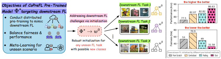
Figure 1: (Left): Overview of CoPreFL, aiming to provide a robust initialization for any unseen downstream FL task. (Right): Average accuracy and variance of FL initialized by various pre-trained models. Centralized pre-training achieves limited performance as it is not able to capture the diverse characteristics of FL settings. CoPreFL demonstrates improved performance in terms of both accuracy and fairness by strategically mimicking downstream FL scenarios during pre-training.

Challenges and goals. As shown in Figure 1, we are interested in developing a methodology that provides robust pre-trained models for FL settings, in the sense of serving as good initializations for any future downstream FL task. This problem poses several challenges. Firstly, the initialization must enhance performance without introducing large accuracy variance among clients in the downstream FL tasks, to address fairness concerns. Secondly, the initialization should effectively handle unseen data and labels, since data available for pre-training could potentially have significant differences from downstream FL tasks due to time-varying environments (e.g., a self-driving car encountering previously unseen objects to classify), new clients joining the system (e.g., face/speech recognition for new phone users), or other factors. This necessitates an initialization that must generalize well to unfamiliar classes/data, accommodating shifts in the task domain or objectives. Lastly, a robust initialization should be versatile, offering a solid starting point across as many FL tasks as possible, to ensure its applicability across various scenarios in FL (see Figure 1).

Addressing these challenges for distributed pre-training scenario is becoming crucial and aligns with many practical settings. For one, the dataset in the pre-training phase is not always centrally available, e.g., due to privacy or communication cost constraints. Despite a centrally stored public large-scale dataset being available during pre-training, the challenges persist, as we see from the centralized result in Figure 1. Considering that the downstream tasks will in turn be trained in an FL setting, FL-based pre-training can more closely resemble the downstream scenario, providing representations that better resonate with target deployment environments. This leads to our key research question:

• How can we design a pre-training strategy that addresses the performance-fairness tradeoff, data heterogeneity, and unseen data/task challenges encountered in downstream FL scenarios?

Overview of methodology and contributions. We propose CoPreFL, a collaborative FL-based pre-training approach for downstream FL tasks. CoPreFL includes several key innovations to address the challenges discussed above. First, for the challenge of mimicking real world scenarios faced in downstream FL, CoPreFL begins by leveraging pre-training data in two common distributed scenarios: (i) one where data is solely available at distributed clients and (ii) another where, in addition to clients holding data, the server also possesses a portion of the dataset. Second, to handle the unseen data challenge, we develop a model-agnostic meta-learning (MAML) approach to enable model adaptation to distributions not encountered during pre-training via meta-updates. Finally, to address the fairness concerns in downstream FL, we encode a balance between performance and variance into the meta-loss optimization objective, rather than solely optimizing based on performance. Our key contributions in developing CoPreFL are:

• We systematically examine how to initialize models for downstream FL tasks, relaxing the assumption that all pre-training data must/should be stored centrally. To this end, we develop a viable approach for pre-training in a hybrid distributed server-client data storage setting, covering scenarios where (i) only clients hold data or where (ii) the server also retains a portion of the data.

• As a component of our methodology, we develop a meta-learning scheme to mimic heterogeneity and dynamics in distributed downstream scenarios, and optimize the pre-trained model for both average accuracy and fairness. This provides robust initializations that implicitly address challenges arising due to any unforseen/evolving downstream FL task.

• We conduct extensive experiments considering several permutations of pre-training setups and different downstream FL tasks. Compared with various centralized and distributed pre-training baselines, our experiments show that CoPreFL consistently offers remarkable improvements in both average performance and fairness across clients for any downstream FL task.

It is also worth mentioning that several existing works utilize meta-learning in an FL setup for personalization (Chen et al., 2018; Jiang et al., 2019; Fallah et al., 2020), but our approach differs in purpose and approach from these works. Since our focus is on downstream FL tasks instead of client-level personalization, we take a different technical approach by meta-updating the global model during pre-training. As we will see in Section 4, this leads to significant performance improvements when clients in the downstream tasks are aiming to collaboratively train a global model via FL. To the best of our knowledge, our work is one of the first to consider FL in both the pre-training and downstream stages. In doing so, we introduce several unique characteristics including hybrid client-server learning and balancing between average performance and fairness during pre-training.

2 Related Work

Pre-training for FL. While pre-training has been extensively applied in AI applications for the centralized setup (Radford et al., 2019; Brown et al., 2020; Devlin et al., 2019; Dosovitskiy et al., 2021; Chu et al., 2024), its potential effects on FL have remained relatively unexplored. A few recent works have studied the effect of model initialization in FL (Nguyen et al., 2023; Chen et al., 2023) by comparing randomly initialized models with centrally pre-trained models. They showed that conducting FL initialized from such models – either publicly available models, or obtained from centralized pre-training on publicly available data – can significantly enhance the model performance. However, as observed in Figure 1, such initialization strategies introduce performance variance challenges and even limited accuracy in downstream FL tasks, since they are not able to mimic multiple downstream FL settings. Compared to these works, we develop a new pre-training strategy tailored to distributed downstream settings, so that initializing FL with the pre-trained model can address the challenges of heterogeneous/unseen data and performance fairness encountered when generalizing across heterogeneous FL deployments.

Meta-learning in FL. Our federated pre-training approach employs meta-learning techniques to adapt the model toward balancing performance and fairness objectives. This distinguishes it from other FL methods that have employed meta-learning, such as personalized FL and few-round FL. Park et al. (2021) introduced few-round FL, which employs a meta-learning-based episodic training strategy to adapt FL to any group within only a few rounds of FL. However, in (Park et al., 2021), fairness is not considered in downstream FL tasks, and no solution is provided for the practical scenario in which the server may hold a proxy dataset. In personalized FL (Chen et al., 2018; Jiang et al., 2019; Fallah et al., 2020; Chu et al., 2022), the global model re-defined through a meta-function which encapsulates gradient updates at each participant. The obtained global model serves as an initialization at each client to achieve a personalized local model through a limited number of gradient descent steps on its own dataset. Unlike this research direction, our emphasis is on establishing an initial model that results in a high-accuracy and equitable global model for downstream tasks that themselves are trained through FL setups. Our collaborative pre-training approach and meta-learning strategy thus differ from these existing works, leading to significant performance improvements as we will observe in Section 4.

Performance fairness in FL. Performance fairness has been studied in the FL literature (Mohri et al., 2019; Li et al., 2020; Cho et al., 2022), aiming to construct a global model that satisfies as many clients as possible (e.g., achieving a uniform distribution of accuracy across participants). One advantages of such models is that, when properly constructed, they are more likely to satisfy the new clients joining the FL system without additional model training. The primary objective of our pre-training method is to construct a robust initial model that guarantees performance and equity for all participants in any downstream FL scenario.

3 Proposed Pre-Training Methodology

In this section, we develop CoPreFL, our meta-learning based pre-training approach, simulating the conditions that could be encountered when applying a pre-trained model to the downstream FL task.

3.1 Problem Setup and Objectives

Federated learning: downstream tasks. Our pre-training approach aims to serve several downstream FL tasks. In each downstream task, a central server is connected to a set of clients $G$. Starting from the initialized model $w^{0}$, each FL task iterates between parallel local training at the clients and global aggregations at the server, across multiple communication rounds. In each downstream training round $r$, every client $g\in G$ downloads the previous global model $w^{r-1}$ from the server and subsequently updates it through multiple iterations of stochastic gradient descent (SGD) using their local dataset, denoted $D_{g}$. After all clients have completed their local model updates, the updated local models, denoted $w^{r}_{g}$, are uploaded to the server for aggregation. This aggregation results in a new global model $w^{r}=\sum_{g\in G}\frac{|D_{g}|}{|D|}w^{r}_{g}$ assuming FedAvg (McMahan et al., 2017) is employed, where $D$ represents the aggregated training set comprising data from all clients and $|D|$ denotes the number of samples in dataset $D$. This entire process is iterated for $R$ communication rounds until convergence.

Pre-training scenarios. As discussed, in this paper, we depart from the convention of centralized pre-training, considering a practical yet challenging scenario in which data samples are distributed across the clients even during the pre-training stage. Here, the labels and data that appear in the pre-training stage are potentially different from the ones that will appear in the downstream FL tasks. We explore two distinct FL scenarios in our analysis during pre-training:

1. Scenario I: The conventional scenario encountered in FL where pre-training datasets are exclusively available at the clients.

2. Scenario II: A hybrid scenario in which the server also holds a small amount of data for pre-training.

Scenario II emulates real-world settings where the entity responsible for creating the machine learning model manages the server and holds a limited dataset that reflects the broader population distribution (e.g., a self-driving car manufacturer with a data store of images encountered on roadways). Such hybrid FL strategies that combine the abundant client data with a relatively small portion of server data are becoming increasingly popular (Yang et al., 2023; Bian et al., 2023).

CoPreFL objectives. Instead of randomly initializing the starting model for downstream FL task, our objective is to design a pre-trained model $\Phi^{*}$ under both scenarios I and II, that serves as a robust starting point $w^{0}=\Phi^{*}$ for any unseen downstream FL task, as shown in Figure 1. More precisely, one of the goals of $\Phi^{*}$ is to minimize the following objective function for downstream FL tasks:

$$A(\Phi)=\mathbb{E}_{G\sim p(\mathcal{G})}\biggl{[}\frac{1}{|G|}\sum_{g\in G}f(w^{R}(\Phi^{*},G),D_{g})\biggr{]},$$ (1)

where $p(\mathcal{G})$ represents the probability distribution of all possible sets of clients comprising any downstream FL task, $G$ is a specific group of clients (i.e., a specific task) drawn from $p(\mathcal{G})$, $f(\cdot)$ represents the loss function, $w^{R}(\Phi^{*},G)$ symbolizes the final $R$-th round global model derived from clients in set $G$ starting from $\Phi^{*}$ as initialization, and $D_{g}$ represents the local dataset of client $g$. The metric in (1) represents the average FL performance across all clients that could possibly appear in the downstream tasks.

On the other hand, FL settings risk producing significant variations in performance among different clients, particularly when the model exhibits bias towards those with larger datasets. This fairness can be assessed by quantifying the variance in testing accuracy across participants (Li et al., 2020). Therefore, besides achieving performance gains on any unseen FL task, we also aim for the final global model $w^{R}(\Phi^{*},G)$ initialized from our designed pre-trained model $\Phi^{*}$ to exhibit a fair testing performance distribution across $|G|$ clients. Specifically, our second objective in designing $\Phi^{*}$ is to minimize the variance of the prediction distribution across participants in downstream FL tasks, i.e.,

$$\begin{split}F(\Phi)&=\mathbb{E}_{{G}\sim p(\mathcal{G})}\biggl{[}\frac{1}{|G|}\sum_{g\in{G}}f^{2}(w^{R}(\Phi^{*},G),D_{g})\\ &-\Big{(}\frac{1}{|G|}\sum_{g\in{G}}f(w^{R}(\Phi^{*},G),D_{g})\Big{)}^{2}\biggr{]}.\end{split}$$ (2)

CoPreFL overview. We aim to strike a balance between (1) and (2). However, we encounter challenges because $D_{g}$, $G$, and $p(\mathcal{G})$ are not known during pre-training, preventing us from directly optimizing $A(\Phi)$ and $F(\Phi)$. To address this, our methodology will employ meta-learning during pre-training to simulate data heterogeneity and dynamics in downstream FL scenarios. We find that this leads to pre-trained models capable of providing robust initialization for any unseen downstream FL task, considering (1) and (2).

To achieve this, we construct a pre-training environment mirroring the federated setup, facilitating the pre-trained model’s ability to account for data heterogeneity across clients and tasks. Our meta-learning-based CoPreFL updates the pre-trained model iteratively over federated rounds using a support set, followed by a concluding adjustment (meta-update) using a query set. By treating the query set as unseen knowledge, our pre-trained model has the capability to effectively handle unforeseen FL scenarios in downstream tasks while striking a balance between (1) and (2).

3.2 CoPreFL in Scenario I (Pre-training with Distributed Clients)

Algorithm 1 Our Pre-training Method CoPreFL (Pre-training Phase in Scenario I)

1:  Input: A set of clients $M$ in the pre-training phase, with each client $i$ holding its pre-training dataset $D^{p}_{i}$.

2:  for Each pre-training communication round $t=1,2,...,T$ do

3:    Randomly select a set of clients $m\subset M$ to participate in learning

4:    Each participant $j\in m$ partitions its own dataset $D^{p}_{j}$ into support set $S_{j}$ and query set $Q_{j}$

5:    for Each participant $j$ in parallel do

6:       Download $\Phi^{t-1}$ from the server

7:       $\mathcal{L}_{S_{j}}(\Phi^{t})$ $\leftarrow$ $\frac{1}{|S_{j}|}$ $\sum_{(x,y)\in S_{j}}{}\ell(\Phi^{t-1}(x),y)$ {// Compute local loss using support set $S_{j}$}

8:       $\Phi^{t}_{j}$ $\leftarrow$ $\Phi^{t-1}$ $-$ $\eta\nabla\mathcal{L}_{S_{j}}(\Phi^{t})$ {// Perform SGD local update using support loss $\mathcal{L}_{S_{j}}$}

9:    end for

10:    $\overline{\Phi^{t}}$ $\leftarrow$ $\sum_{j\in m}\frac{|S_{j}|}{\sum_{i\in m}|S_{i}|}\Phi^{t}_{j}$ {// Model aggregation to construct temporary global model}

11:    for Each participant $j$ in parallel do

12:       Downloads $\overline{\Phi^{t}}$ from the server

13:       $\mathcal{L}_{Q_{j}}(\overline{\Phi^{t}})$ $\leftarrow$ $\frac{1}{|Q_{j}|}$ $\sum_{(x,y)\in Q_{j}}{}\ell(\overline{\Phi^{t}}(x),y)$ {// Compute local loss (and gradient) using query set $Q_{j}$}

14:    end for

15:    Overall query meta-loss: $\mathcal{L}_{Q}(\overline{\Phi^{t}})=\sum_{j\in m}\mathcal{L}_{Q_{j}}(\overline{\Phi^{t}})$; Variance across meta-losses: $\sigma_{Q}^{2}(\overline{\Phi^{t}})$

16:    $\mathcal{L}_{meta}(\overline{\Phi^{t}})=\gamma\mathcal{L}_{Q}(\overline{\Phi^{t}})+(1-\gamma)\sigma_{Q}^{2}(\overline{\Phi^{t}})$ {// Compute customized query meta-loss}

17:    $\Phi^{t}$ $\leftarrow$ $\overline{\Phi^{t}}$ $-$ $\zeta\nabla\mathcal{L}_{meta}(\overline{\Phi^{t}})$ {// Meta-learning model update using customized loss}

18:  end for

19:  Output: A pre-trained model for downstream FL tasks: $\Phi^{T}$

We first consider the scenario where pre-training data is collected from $M$ distributed clients, and no data is stored on the server. The detailed procedure of CoPreFL for this case is given in Algorithm 1. To start, in each round of pre-training, each participant $j$ splits its local pre-training dataset $D^{p}_{j}$ into support set $S_{j}$ and query set $Q_{j}$, which are disjoint. This division will help our meta-learning maximize the model’s generalization ability in unseen downstream scenarios.

Temporary global model construction. In each FL round $t$ of pre-training, we randomly select $m\subset M$ participants to download $\Phi^{t-1}$ from the server (line 6 in Algorithm 1). Subsequently, clients engage in a series of local training iterations using their respective support sets $S_{j}$ (line 7 in Algorithm 1), resulting in a training support loss $\mathcal{L}_{S_{j}}(\Phi^{t})=\frac{1}{|S_{j}|}\sum_{(x,y)\in S_{j}}{}\ell(\Phi^{t-1}(x),y)$, where $\ell(\cdot)$ denotes the loss function applied to the model’s input $x$ and target $y$ (e.g., cross-entropy loss). Participants then update their local models using the loss $\mathcal{L}_{S_{j}}(\Phi^{t})$ to obtain $\Phi^{t}_{j}$ (line 8). The updated models are aggregated at the server (line 10) according to $\overline{\Phi^{t}}=\sum_{j\in m}\frac{|S_{j}|}{\sum_{i\in m}|S_{i}|}\Phi^{t}_{j}$. This model can be viewed as the temporary global model that will be further refined using the query sets. Note that our emphasis is on crafting an initial model that can establish a robust “global model” during downstream tasks, requiring updates to this temporary global model.

Measuring performance and fairness. Next, the query sets are used to evaluate the model’s performance on each client and to conduct the meta-update process. CoPreFL aims to strike a balance between the following functions during the pre-training phase:

$$\min_{\Phi}\mathcal{L}_{Q}(\overline{\Phi^{t}})=\min_{\Phi}\sum_{j\in m}\mathcal{L}_{Q_{j}}(\overline{\Phi^{t}})\text{ and}$$ (3)

$$\min_{\Phi}\sigma_{Q}^{2}(\overline{\Phi^{t}})=\min_{\Phi}\frac{1}{|m|}\sum_{j\in m}\Big{(}\mathcal{L}_{Q_{j}}(\overline{\Phi^{t}})-\frac{1}{|m|}\mathcal{L}_{Q}(\overline{\Phi^{t}})\Big{)}^{2},$$ (4)

where $\mathcal{L}_{Q_{j}}$ represents the loss evaluated using the query set $Q_{j}$ of participant $j$, $\mathcal{L}_{Q}$ denotes the overall query loss, which is characterized by aggregating $\mathcal{L}_{Q_{j}}$ across all participants, and $\sigma_{Q}^{2}$ represents the performance variance evaluated using the query set across participants. Based on this, to capture the performance-fairness tradeoff, we construct a customized query meta-loss function $\mathcal{L}_{meta}(\overline{\Phi^{t}})$ to minimize not only the overall query loss $\mathcal{L}_{Q}(\overline{\Phi^{t}})$ when encountering unseen data, but also the variance $\sigma_{Q}^{2}(\overline{\Phi^{t}})$ of query losses across participants:

$$\min_{\Phi}\mathcal{L}_{meta}(\overline{\Phi^{t}})=\min_{\Phi}\left[\gamma\mathcal{L}_{Q}(\overline{\Phi^{t}})+(1-\gamma)\sigma_{Q}^{2}(\overline{\Phi^{t}})\right],$$ (5)

where $\gamma\in[0,1]$ represents a controllable balancer between the average performance and fairness. Setting $\gamma=0$ encourages a more uniform training accuracy distribution and improves fairness, aligning with (4), but may sacrifice performance. A larger $\gamma$ means that we emphasize the clients’ average performance with less consideration for uniformity, optimizing the pre-trained model more towards (3).

Meta update. Considering the above objective function, each participant $j$ downloads the temporary global model $\overline{\Phi^{t}}$ and employs its query set $Q_{j}$ to compute its local query loss $\mathcal{L}_{Q_{j}}(\overline{\Phi^{t}})=\frac{1}{|Q_{j}|}\sum_{(x,y)\in Q_{j}}{}\ell(\overline{\Phi^{t}}(x),y)$ as in line 13 in Algorithm 1. The gradients are also computed locally and sent back to server, as both are necessary to conduct the meta-update. Subsequently, the overall query meta-loss $\mathcal{L}_{Q}(\overline{\Phi^{t}})$ is computed by aggregating all local query losses, and the performance variance $\sigma_{Q}^{2}(\overline{\Phi^{t}})$ is determined by analyzing query meta-losses across all participants (line 15). Then, as described in line 17 of Algorithm 1, CoPreFL updates the temporary global model $\overline{\Phi^{t}}$ using the customized query meta-loss $\mathcal{L}_{meta}$ and the aggregated received gradients to align with our controlled objective. The server finally broadcasts the meta-updated global model $\Phi^{t}$ to the participants and proceeds to the next round.

After $T$ federated rounds, the final global model $\Phi^{T}$ serves as the pre-trained model for initializing FL in the downstream tasks, i.e., in Figure 1, the set of clients in any downstream task conduct FL starting from the pre-trained model $w^{0}=\Phi^{T}$.

3.3 CoPreFL in Scenario II (Hybrid Client-Server Pre-Training)

We next explore a pre-training scenario where in addition to clients holding the data, the server also possesses a small portion of data drawn from the broader population distribution. Hence, unlike CoPreFL in scenario I where we separated participants’ data into support and query sets, viewing the query sets as unseen knowledge to control average performance and fairness, in scenario II, we employ all samples within each client as support data for local updates. Instead, we treat the server’s data as the query set.

The detailed procedure of CoPreFL in scenario II is given in Algorithm 2 in Appendix B. Here, we highlight the key differences from Algorithm 1. First, the temporary global model $\overline{\Phi^{t}}$ is aggregated from local models trained on the client’s entire local dataset $D^{p}_{j}$. Second, we facilitate the meta-update of the temporary global model $\overline{\Phi^{t}}$ using the server’s data instead of client’s data. Specifically, we randomly partition the server’s dataset $D^{s}$ into $|m|$ equally-sized partitions to help mimic the distributed nature of downstream FL tasks, and furnish distributed clients with a global model suited to our objectives (3) and (4). The temporary global model $\overline{\Phi^{t}}$ is then updated based on a customized meta-loss $\mathcal{L}_{meta}(\overline{\Phi^{t}})$ defined similarly to (5), but calculated through meta-updates on the server’s partitioned data.

Note that unequal and/or non-uniformly random partitionings of the server-side dataset for meta-updating could be considered as alternatives, e.g., to force specific label splits across partitions. However, due to the server’s lack of knowledge about future downstream FL tasks during pre-training, including their dataset sizes, distributions, and dynamics, meta-updating the model with randomly allocated query sets is an intuitive solution. We show in Section 4 that this partitioning provides significant performance improvements over other pre-training strategies.

Remark 1 (Temporary global model). Note that our meta update for each scenario is applied to the temporary global model to mimic downstream FL tasks. This is an important distinction from existing meta-learning based FL methods discussed in Section 2 that meta-update the local models to mimic local/personalized training. This leads to significant performance improvement of CoPreFL compared with employing these existing algorithms as pre-training baselines, as we will see in Section 4.

Remark 2 (Applications to centralized public datasets). Although we presented CoPreFL for two specific distributed pre-training scenarios, CoPreFL is applicable even when all of the pre-training data is centralized at the server (e.g., public datasets). The server can split the dataset to mimic either scenarios I or II, and directly apply the above training strategies. We will show in Section 4 that CoPreFL obtains advantages over standard centralized pre-training even in these settings, since it provides an initialization better prepared for downstream heterogeneity.

4 Experiments

4.1 Experimental Setup

Dataset and model. We conduct image classification using CIFAR-100 (Krizhevsky, 2009), Tiny-ImageNet (Le & Yang, 2015), and FEMNIST (Caldas et al., 2018), adhering to the data splits provided in (Ravi & Larochelle, 2016; Park et al., 2021), and adopt ResNet-18 (He et al., 2015). For CIFAR-100, the dataset is divided into 80 classes for pre-training and 20 classes for downstream FL tasks, while for Tiny-ImageNet, the dataset is separated into 160 classes for pre-training and 40 classes for downstream FL tasks. This models a practical scenario where downstream task labels are unknown during pre-training. Additionally, we will explore mixed scenarios where there are overlapping classes between pre-training and downstream tasks. By default, we randomly select 95% of the samples from the pre-training dataset to form the dataset for clients, while the remaining 5% of samples constitute the server dataset. For FEMNIST, we report the detailed settings and results in Appendix D.4.

Pre-training phase. We distribute the pre-training dataset to $|M|=100$ clients following non-IID data distributions and select $|m|=20$ participants out of the $|M|$ clients to participate in each FL round. Results with different $|m|$ and IID setups are reported throughout Appendix D. Each participant employs 80% of its local data as support samples and the remaining 20% as query samples. We set the number of global rounds to $T=50$, and each round of local training takes 5 iterations for each participant. See Appendix C.1- C.2 for detailed hyperparameters and compute settings.

Downstream FL task and evaluation metrics. As illustrated in Figure 1, the final global model of the pre-training phase is utilized as the initialization for each downstream FL task, where we consider multiple downstream tasks to evaluate the overall performance. To generate each downstream FL task, we randomly select 5 classes out of the 20 classes from the CIFAR-100 dataset and 40 classes from the Tiny-ImageNet dataset, and distribute the corresponding data samples to $|G|=10$ clients following non-IID data distributions (see Appendix D for IID results). Each participant in the downstream phase utilizes 80% of its local data as training samples, while the remaining 20% is reserved for testing samples. To focus on the impact of different pre-training methods to FL, we keep the training procedure consistent for each downstream task, using the widely used FedAvg algorithm (see Appendix C.2 for detailed settings). We evaluate the final global model’s performance using test samples from each participant and report both the accuracy and the variance of the accuracy distribution across $|G|$ clients for each FL task. We consider a total of $X=10$ downstream FL tasks, and the evaluation metrics are reported as the average across these different tasks.

Data distribution. Data samples from each class are distributed to $|M|=100$ clients for pre-training and $|G|=10$ clients for downstream FL tasks using the corresponding dataset based on a Dirichlet($\alpha$) distribution with $\alpha=0.5$, as done in the literature (Morafah et al., 2022; Li et al., 2021).

Pre-training	Downstream: Non-IID FedAvg (CIFAR-100)					Downstream: Non-IID FedAvg (Tiny-ImageNet)
Method	Acc $\uparrow$	Variance $\downarrow$	Worst 10% $\uparrow$	Worst 20%$\uparrow$	Worst 30% $\uparrow$	Acc $\uparrow$	Variance $\downarrow$	Worst 10% $\uparrow$	Worst 20% $\uparrow$	Worst 30% $\uparrow$
FedAvg	78.96	64.80	62.70	67.00	69.80	82.94	37.21	68.99	72.29	74.40
FedMeta	82.45	48.72	68.97	72.41	74.35	81.03	37.58	69.44	71.55	72.93
q-FFL	80.01	88.92	64.39	67.48	70.30	84.11	43.96	73.87	76.05	77.37
CoPreFL	83.29	34.69	71.58	73.20	74.59	85.23	35.40	76.77	78.46	79.86

(a) Results in scenario I using CIFAR-100 and Tiny-ImageNet datasets.

Pre-training	Downstream: Non-IID FedAvg (CIFAR-100)					Downstream: Non-IID FedAvg (Tiny-ImageNet)
Method	Acc $\uparrow$	Variance $\downarrow$	Worst 10% $\uparrow$	Worst 20% $\uparrow$	Worst 30% $\uparrow$	Acc $\uparrow$	Variance $\downarrow$	Worst 10% $\uparrow$	Worst 20% $\uparrow$	Worst 30% $\uparrow$
FedAvg	82.82	49.00	69.71	72.54	74.58	82.87	48.16	68.94	72.91	75.28
FedMeta	82.69	48.44	68.84	71.82	74.14	84.19	49.70	70.41	72.63	74.74
q-FFL	82.14	73.10	68.22	70.64	73.77	83.51	44.22	69.91	73.71	76.01
CoPreFL-SGD	83.63	41.73	69.76	73.46	75.64	84.30	36.24	72.83	75.64	77.37
CoPreFL	86.63	31.58	73.05	75.82	77.58	84.72	24.80	75.84	77.31	78.50

(b) Results in scenario II using CIFAR-100 and Tiny-ImageNet datasets.

Table 1: Average performance across 10 different non-IID downstream FL tasks, initialized with various non-IID FL pre-trained methods. CoPreFL provides the best initialization for downstream FL scenarios on all metrics.

Baselines for pre-training. We compare CoPreFL with various established FL algorithms, including standard FedAvg (McMahan et al., 2017), FedMeta (Chen et al., 2018), which addresses the unseen scenario through meta-learning, and q-FFL(q $>$ 0) (Li et al., 2020), which aims at enhancing performance fairness across clients. For fair comparison, all schemes are adopted during the pre-training to construct initial models under the same setting. When applying these baselines in scenario II, after the global model is constructed in each round, we proceed to further train the global model with 5 additional iterations on the server dataset. This extended training follows the approach in (Yang et al., 2023; Bian et al., 2023), where the server’s data is used to further refine the global model. Similarly, we introduce a baseline called CoPreFL-SGD, which first constructs a global model according to Algorithm 1 and then further performs SGD iterations using server data on the global model. Finally, we also consider initializations based on random weights, conventional centralized pre-training, and additional FL algorithms (in Table 3 and Appendix D.5).

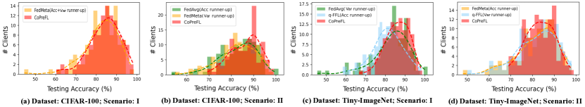
Figure 2: Testing accuracy distributions in different non-IID FL downstream tasks. CoPreFL achieves the best average accuracy and a narrower (i.e., fairer) distribution while also improving the accuracies of worst performing clients.

4.2 Experimental Results

Results for scenario I. Table 1(a) shows test accuracies averaged over 10 different non-IID FL downstream tasks, initialized with various pre-trained methods in scenario I on the CIFAR-100 and Tiny-ImageNet datasets. We see that our pre-trained method CoPreFL offers a robust initialization that is characterized by higher average accuracy and reduced variance across clients in downstream FL tasks. Moreover, CoPreFL also increases accuracies for the worst-performing clients, as indicated by the Worst 10-30% metrics. This further highlights the advantage of balancing the two objective functions (3) and (4), particularly in benefiting the worst-performing clients. See Appendix D.1 for supplemental results considering varying the number of participants in pre-training as well as different data distributions in downstream FL tasks for scenario I.

Results for scenario II. Table 1(b) displays the performance of various pre-trained methods trained in scenario II. Once again, CoPreFL outperforms other baselines, demonstrating that utilizing server data for meta-updates and striking a balance between objectives (3) and (4) with the server’s data can still effectively align with goals (1) and (2). We observe that CoPreFL consistently outperforms CoPreFL-SGD, indicating that conducting a few SGD iterations using server data in a centralized manner after meta-updating the global model might diminish the effectiveness of our designed objectives. This further emphasizes the importance of performing meta-learning on the server data following the partitioning outlined in Algorithm 2 for scenario II. See Appendix D.2 for results considering different configurations.

Fairness of CoPreFL. Figure 2 depicts the testing accuracy distributions of the final global model on each client in downstream tasks. We provide visualizations for our method, as well as the methods with the second-best average accuracy and the second-lowest variance. CoPreFL achieves both higher average accuracies compared to other pre-training methods, as well as narrower (i.e., fairer) accuracy distributions with reduced variances. Moreover, CoPreFL effectively shifts low-performing clients on the left towards the right, signifying an enhancement in accuracy for these clients. We provide additional visual results across different scenarios in Appendix D.3.

$\gamma$ of CoPreFL	Acc $\uparrow$	Variance $\downarrow$
0.0	83.11	24.70
0.25	84.04	35.88
0.5	85.23	35.40
0.75	85.19	39.31
1.0	86.33	39.81

Table 2: Effect of $\gamma$ in scenario I, using Tiny-ImageNet.

Effect of balancer $\gamma$ in CoPreFL. Table 2 gives the performance obtained from initializing with CoPreFL using different balancers $\gamma$ on Tiny-ImageNet. A larger $\gamma$ implies that the pre-trained model prioritizes the devices’ average performance, whereas a smaller $\gamma$ implies that the pre-trained model aims to improve fairness. In Table 2, as the balancer $\gamma$ increases, we observe an increase in the average accuracy of downstream FL tasks but a decrease in fairness, indicated by higher variance. The trend shows that CoPreFL establishes a robust pre-training environment that mimics downstream FL tasks while allowing control over the relative importance between accuracy and fairness.

Pre-training (Scenario I)	Downstream: Non-IID FedAvg
Method	Acc $\uparrow$	Variance $\downarrow$
Random Initialization	75.32	41.39
Centralized (Nguyen et al., 2023)	81.30	69.44
SCAFFOLD (Karimireddy et al., 2019)	79.15	57.84
FedDyn (Acar et al., 2021)	81.23	53.17
PerFedAvg (Fallah et al., 2020)	81.58	49.73
CoPreFL	83.29	34.69

Table 3: Results with other initializations on CIFAR-100.

Comparison with other initialization methods. In addition to the baselines in Table 1(b) which incorporate fairness or meta-learning, in Table 3, we also consider the popular SCAFFOLD (Karimireddy et al., 2019), FedDyn (Acar et al., 2021), and PerFedAvg (Fallah et al., 2020) algorithms for pre-training. We see that CoPreFL outperforms these baselines as well, demonstrating that a proper pre-training design based on (3) and (4) can indeed enhance FL through initialization. The other FL algorithms are not as well equipped to handle unseen dynamics and performance fairness during pre-training. Moreover, besides FL algorithms, we also consider random weights and a centrally pre-trained model, a concept introduced in (Nguyen et al., 2023), for initializing downstream FedAvg. While the centralized method improves the accuracy of downstream FL compared to random initialization, it introduces significant variance across clients, resulting in fairness issues due to inability to mimic downstream FL characteristics. More details along with additional results can be found in Appendix D.5.

Pre-training (Scenario I)	Downstream: Non-IID FL
	FedProx ($\mu$ = 1)		q-FFL (q = 2)
Method	Acc $\uparrow$	Variance $\downarrow$	Acc $\uparrow$	Variance $\downarrow$
Centralized	82.39	51.46	79.26	47.10
FedAvg	79.53	46.15	79.53	44.59
FedMeta	81.77	63.12	79.30	39.63
q-FFL	83.19	52.12	81.38	37.27
CoPreFL	84.31	30.55	82.71	25.39

Table 4: Applications of other FL algorithms during downstream scenarios on CIFAR-100.

Implementation using other downstream FL algorithms. We next explore the ability of our pre-training method to enhance the performance of downstream FL algorithms other than FedAvg. For this, we consider FedProx (Sahu et al., 2018) and fairness-aware q-FFL (Li et al., 2020). Table 4 shows the results. Overall, we see that CoPreFL consistently achieves superiority in accuracy and variance for different downstream FL algorithms compared to other pre-training baselines. Details on the implementation and further discussions are provided in Appendix D.6.

Both unseen/seen classes in downstream FL tasks. In addition to the setting without overlapping classes between pre-training and downstream tasks, we explore a mixed scenario where clients in the downstream FL task also hold “seen classes.” To implement this, we randomly sampled 10 classes from the pre-training dataset and 10 classes from our CIFAR-100 downstream dataset, resulting in 20 classes total with 10 seen and 10 unseen. To construct each downstream scenario, we randomly selected 5 classes to conduct non-IID downstream FedAvg, and repeated this 10 times. The pre-trained models were solely trained on the original 80 classes of CIFAR-100. Table 5 shows the results. We see that the accuracies are generally higher compared to those in Table 1(a), as the downstream tasks involve classes seen during pre-training. Also, the observed trends compared with the baselines further align with the outcomes for only unseen classes, confirming the advantage of CoPreFL.

Pre-training	Downstream: Non-IID FedAvg
Method	Acc $\uparrow$	Var $\downarrow$	Worst 10%	Worst 20%	Worst 30%
Centralized	82.63	63.57	67.35	69.22	70.38
FedAvg	80.19	51.35	68.72	70.15	72.33
FedMeta	83.14	39.85	67.29	71.35	73.81
q-FFL	81.34	47.98	69.22	70.35	72.37
CoPreFL	84.79	30.51	70.83	72.66	74.10

Table 5: Results with both seen/unseen classes during downstream FL. CIFAR-100 is adopted in pre-training scenario I.

Pre-training	Downstream: Non-IID FedAvg
Method	Acc $\uparrow$	Variance $\downarrow$
Centralized	86.75	67.34
CoPreFL	87.96	30.79

Table 6: Results with pre-training on a centrally stored public dataset. ImageNet is used for pre-training, while CIFAR-100 is used for downstream FL.

Application to centrally stored large public dataset. Finally, we further consider the applicability of CoPreFL when a large dataset is available and centrally stored. To achieve this, we performed pre-training using the ImageNet_1K dataset and used FedAvg as the downstream task with CIFAR-100. Recall from Remark 2 that even when a public large-scale dataset is centrally stored, we can intentionally split the dataset to mimic the distributed nature of downstream FL. The results are shown in Table 6. The superiority in performance and fairness achieved by CoPreFL further confirms the advantage and applicability of our approach to different scenarios. Detailed implementations and additional results can be found in Appendix D.7.

5 Conclusion

We presented CoPreFL, a collaborative pre-training method that provides a robust model initialization for downstream FL tasks. CoPreFL leverages meta-learning to equip the pre-trained model with the ability handle unseen dynamics and heterogeneity in FL scenarios, while balancing between performance and fairness. We showed how our pre-training approach can be applied to different scenarios of data samples being distributed among clients and the server, or even when all samples are centrally stored. Extensive experiments demonstrated the advantages of CoPreFL compared with baselines in initializing downstream FL tasks.

Appendix A Key Applications

Consider a healthcare application where each client, such as a hospital or an individual patient, aims to build a comprehensive global model capable of classifying a wide range of diseases. However, individual clients may possess limited types of diseases in their local datasets – for instance, one client may have data on diseases A and B but lacks information on diseases C and D. In this context, federated learning becomes essential. Clients need to collaborate to construct a global model that not only reflects the diseases available locally but also incorporates information about diseases not present in their individual datasets, ensuring a more robust and universally applicable healthcare model.

Similarly, in the domain of autonomous vehicles, each self-driving car may strive to develop a global model for scenario detection in various weather conditions. However, individual cars might encounter limited weather scenarios locally – one car might navigate through a desert environment, while another faces challenges in a snowy storm. Through federated learning, these cars can collectively construct a global model that accounts for a broad spectrum of weather conditions, ensuring robust scenario detection capabilities for all vehicles involved.

As noted in Remark 2, the server can intentionally partition the centralized dataset and implement our scheme, utilizing multiple computing units available at the server, to obtain a pre-trained model. The advantage of this approach, compared to simple centralized training, lies in mitigating side effects such as performance biases and the substantial variance associated with centralized training. This phenomenon stems from the lack of generalizability in the model’s design. When a model undergoes pre-training in a centralized manner based on SGD, it becomes rigidly bound to the knowledge in the pre-training dataset. This fixation presents a challenge in adapting the model to the diverse clients that may possess new or unseen data in downstream tasks. Such variations can arise from factors like the time-varying environment or new clients joining the system, as exemplified in the aforementioned applications: classifying different scenarios based on the self-driving car’s environment, identifying diverse diseases based on patient interests, or enabling face/speech recognition for new phone users.

In our experimental comparison, we consider a FL baseline, FedMeta (Chen et al., 2018), which also incorporates meta-learning. We would like to emphasize that the distinction between our CoPreFL and FedMeta lies in the application, which requires us to conduct meta-update in a totally different way. FedMeta is designed to offer personalization to individual clients, e.g., when a specific client is interested in predicting only diseases A and B, or when a specific self-driving car is interested in the model tailored to a specific weather. In contrast, our emphasis is on creating an initial model that can construct a good “global model” during downstream instead of “personalized models”, targeting the aforementioned applications. This is the reason why we need to update the temporary global model instead of the local models, which is the key technical difference with FedMeta. Another technical difference is the consideration of fairness in our method. These two key techniques enables CoPreFL to construct a robust initial model that can quickly adapt to “any group of clients” (instead of individual clients) to construct a global model during downstream tasks.

Appendix B Detailed Procedure for CoPreFL in Scenario II

This section provides a detailed introduction to our CoPreFL in scenario II, as discussed in Section 3.3. Similar to the goals of CoPreFL in scenario II, we still aim to balance between objective functions (3) and (4), but in this scenario, the data used to perform meta-updates and control our objectives is different. During each federated round $t$ in the pre-training phase, participants download the global model $\Phi^{t-1}$ from the previous round (line 6 in Algorithm 2). Subsequently, they perform few local training iterations utilizing their respective local datasets $D^{p}_{j}$ (line 7 in Algorithm 2). This process leads to a training loss $\mathcal{L}_{D^{p}_{j}}(\Phi^{t})$, defined as $\frac{1}{|D^{p}_{j}|}$ $\sum_{(x,y)\in D^{p}_{j}}{}\ell(\Phi^{t-1}(x),y)$, where $x$ represents the input (e.g., images), $y$ denotes the true label, and $\ell(\cdot)$ denotes the loss function (e.g.,cross-entropy loss). The local models are then updated based on this loss, yielding their respective updated local models $\Phi^{t}_{j}$ (line 8 in Algorithm 2). Upon the completion of local training by all participants, participants’ local models are transmitted to the server (line 10 in Algorithm 2), and the server aggregates these models into a temporary global model $\overline{\Phi^{t}}=\sum_{j\in m}\mu_{j}\Phi^{t}_{j}$, which is weighted by relative dataset sizes $\mu_{j}=\frac{|D^{p}_{j}|}{\sum_{i\in m}|D^{p}_{i}|}$.

We then perform meta-updates on the temporary global model $\overline{\Phi^{t}}$ using server’s dataset $D^{s}$. To start, we first randomly divide the server’s dataset $D^{s}$ into $|m|$ equal partitions. Instead of equal partitioning, one can also divide the server-side dataset into partitions with unequal sizes and use them for meta-update. However, during pre-training, the server does not know the dataset sizes of clients in future downstream tasks. In this case, one intuitive way is to treat all clients equally/fairly, by meta-updating the model with the same query set sizes. We show that this equal partitioning provides significant performance improvements as can be seen in our experiments. Subsequently, the server evaluates the temporary global model $\overline{\Phi^{t}}$ using each subset $D^{s}_{j}$ (line 12 in Algorithm 2), resulting in the corresponding gradient and loss $\mathcal{L}_{D^{s}_{j}}(\overline{\Phi^{t}})$ = $\frac{1}{|D^{s}_{j}|}$ $\sum_{(x,y)\in D^{s}_{j}}{}\ell(\overline{\Phi^{t}}(x),y)$. The collective server’s loss, denoted as $\mathcal{L}_{D^{s}}(\overline{\Phi^{t}})$ in line 14 of Algorithm 2, is determined by aggregating all the collected loss values obtained from $D^{s}_{j}$, and we also calculate the variance $\sigma_{D^{s}}^{2}=\frac{1}{m}\sum_{i\in m}(\mathcal{L}_{D^{s}_{i}}(\overline{\Phi^{t}})-\frac{1}{m}\mathcal{L}_{D^{s}}(\overline{\Phi^{t}}))$ across server’s losses to examine the performance distribution. We then tailor a customized server meta-loss $\mathcal{L}_{meta}(\overline{\Phi^{t}})=\gamma\mathcal{L}_{D^{s}}(\overline{\Phi^{t}})+(1-\gamma)\sigma_{D^{s}}^{2}(\overline{\Phi^{t}})$ to achieve a balance between optimizing for performance and fairness. Finally, in line 17 of Algorithm 2, we employ the customized server meta-loss $\mathcal{L}_{meta}(\overline{\Phi^{t}})$ and the aggregated gradient gathered from the server’s subsets to update the temporary global model $\overline{\Phi^{t}}$, aligning it with our controlled objective. The server then sends this meta-updated global model $\Phi^{t}$ to the participants in the next round for initialization. After completing $T$ federated rounds, we regard the final global model $\Phi^{T}$ as the pre-trained model in scenario II, which serves as the initialization for the downstream FL tasks.

Algorithm 2 Our Pre-training Method CoPreFL (Pre-training Phase in Scenario II)

1:  Input: $M$ clients in the pre-training phase, with each client $i$ holding their own dataset $D^{p}_{i}$; the server also holds a dataset $D^{s}$.

2:  for Each communication round $t=1,2,...,T$ do

3:     Randomly select a set of client $m\subset M$ to participate in learning

4:     Randomly split server’s dataset $D^{s}$ into $|m|$ subsets

5:     for Each participant $j$ in parallel do

6:        Downloads $\Phi^{t-1}$ from the server

7:        $\mathcal{L}_{D^{p}_{j}}(\Phi^{t})$ $\leftarrow$ $\frac{1}{|D^{p}_{j}|}$ $\sum_{(x,y)\in D^{p}_{j}}{}\ell(\Phi^{t-1}(x),y)$ {// Get local loss using local dataset $D^{p}_{j}$}

8:        $\Phi^{t}_{j}$ $\leftarrow$ $\Phi^{t-1}$ $-$ $\eta\nabla\mathcal{L}_{D^{p}_{j}}(\Phi^{t})$ {// Perform SGD local update using local loss $\mathcal{L}_{D^{p}_{j}}$}

9:     end for

10:     $\overline{\Phi^{t}}$ $\leftarrow$ $\sum_{j\in m}\frac{|D^{p}_{j}|}{\sum_{i\in m}|D^{p}_{i}|}\Phi^{t}_{j}$ {// Model aggregation to construct temporary global model}

11:     for Each split server’s dataset $D^{s}_{j}$ in parallel, Server do

12:        $\mathcal{L}_{D^{s}_{j}}(\overline{\Phi^{t}})$ $\leftarrow$ $\frac{1}{|D^{s}_{j}|}$ $\sum_{(x,y)\in D^{s}_{j}}{}\ell(\overline{\Phi^{t}}(x),y)$ {// Server’s loss corresponding to each partition}

13:     end for

14:     Overall meta-loss on server: $\mathcal{L}_{D^{s}}(\overline{\Phi^{t}})=\sum_{j\in m}\mathcal{L}_{D^{s}_{j}}(\overline{\Phi^{t}})$

15:     Variance across server meta-losses: $\sigma_{D^{s}}^{2}(\overline{\Phi^{t}})=\frac{1}{|m|}\sum_{j\in m}(\mathcal{L}_{D^{s}_{j}}(\overline{\Phi^{t}})-\frac{1}{|m|}\mathcal{L}_{D^{s}}(\overline{\Phi^{t}}))^{2}$

16:     Customized server meta-loss: $\mathcal{L}_{meta}(\overline{\Phi^{t}})=\gamma\mathcal{L}_{D^{s}}(\overline{\Phi^{t}})+(1-\gamma)\sigma_{D^{s}}^{2}(\overline{\Phi^{t}})$

17:     $\Phi^{t}$ $\leftarrow$ $\overline{\Phi^{t}}$ $-$ $\zeta\nabla\mathcal{L}_{meta}(\overline{\Phi^{t}})$ {// Model meta-updates using customized loss}

18:  end for

19:  Output: A pre-trained model for downstream FL tasks: $\Phi^{T}$

Appendix C Detailed Settings for Datasets and Hyperparameters

C.1 Datasets Details

In a practical scenario where labels for downstream tasks are unknown during pre-training, we split the dataset based on classes. For CIFAR-100 (100 classes with 600 images per class), 80 classes are used for pre-training and 20 classes for downstream FL tasks, resulting in 48,000 images for pre-training and 12,000 images for downstream tasks. Similarly, for Tiny-ImageNet (200 classes with 600 images per class), 160 classes are employed for pre-training and 40 classes for downstream FL tasks, providing 96,000 images for pre-training and 24,000 images for downstream tasks. We randomly select 95% of the pre-training dataset samples for clients, while the remaining 5% of samples for the server. Specifically, for CIFAR-100, this results in 45,600 images for clients and 2,400 images for the server. For Tiny-ImageNet, we allocate 91,200 images for clients and 4,800 images for the server. We will distribute 45,600 and 91,200 images to $|M|=100$ clients based on IID or non-IID data distribution for CIFAR-100 and Tiny-ImageNet, respectively. Each client further divides its local data into 80% support samples and 20% query samples.

For the downstream phase samples (12,000 images for CIFAR-100 and 24,000 images for Tiny-ImageNet), we randomly select 5 classes from the available downstream classes (20 classes for CIFAR-100 and 40 classes for Tiny-ImageNet) to form a single FL task. This results in 3,000 images (5 classes with 600 images per class) for each FL task in both CIFAR-100 and Tiny-ImageNet datasets. These 3,000 images are distributed to $|G|=10$ clients based on either IID or non-IID data distribution. Within each client, 80% of local data is used for FL training, while the remaining 20% is reserved to evaluate the final global model.

In the IID setup, data samples from each class are distributed equally to $|M|=100$ clients for pre-training and $|G|=10$ clients for downstream FL task. Taking the CIFAR-100 dataset in the IID pre-training phase as an example, there are $|M|=100$ clients, each holding 456 images. We will randomly select $|m|$ clients to participate in pre-training in each round. In the IID downstream phase of CIFAR-100, there are $|G|=10$ clients, each holding 300 images. In the non-IID setup, samples within each class are partitioned among $|M|$ and $|G|$ clients using a Dirichlet($\alpha$) distribution for pre-training and downstream task, respectively, with $\alpha=0.5$ selected as is in the literature (Morafah et al., 2022; Li et al., 2021).

C.2 Hyperparameters and Compute Settings

We use ResNet-18 as model structure for image classification, following the setting of (Nguyen et al., 2023; Chen et al., 2023). For our method, the SGD optimizer with a learning rate of $\eta=10^{-3}$ and $\zeta=10^{-3}$ is adopted for both local and meta updates. Both local and meta learning rates are searched within the range of [1e-2, 5e-3, 1e-3, 5e-4]. We searched for learning rates within the range of [1e-2, 5e-3, 1e-3, 5e-4] for local training of all FL pre-training baselines and selected 1e-3 as the optimal learning rate for them. In scenario II, each FL baseline will continue to conduct a few SGD iterations using the server’s data after constructing their global model. We searched for learning rates in the range of [1e-2 and 1e-3] for this additional training and selected 1e-3 as the optimal learning rate for the server. Regarding hyperparameters in the q-FFL baseline, we conducted experiments with q-values of 1, 3, and 5 and reported the corresponding best statistics. We select a learning rate $\eta$ from the range [1e-2, 5e-3, 1e-3, 5e-4] for local updates in our CoPreFL and determined that 1e-3 provides the best results. Additionally, for meta-updates in both scenarios, we search for the learning rate $\zeta$ within the range [1e-2, 1e-3] and find that 1e-3 is the optimal value. In the case of the centralized baseline mentioned in Section 4.2, we searched for the optimal learning rate within the range [1e-2, 5e-3, 1e-3, 5e-4, 1e-4], ultimately selecting 1e-3. We utilized the SGD optimizer for all updates across all methods, and the batch size is set to be 32 for all experiments.

For downstream FL tasks, we employ the widely used FedAvg algorithm to isolate the effects of different FL approaches and focus specifically on the impact of different initializations. We consider $R=50$ FL rounds using the training set, involving 5 iterations per round for local training using the SGD optimizer with a learning rate of $10^{-3}$. For the settings of other downstream FL algorithms, see Appendix D.6. In our simulations of CoPreFL, we assessed various balancer values $\gamma$ from the range [0.0, 0.25, 0.5, 0.75, 1.0] in all scenarios during pre-training. For evaluation of downstream FL, we report the best-performing (highest average accuracy) value in our paper. For fair selection/comparison, we also report the results of other baselines with their own best accuracy when searching for hyperparameters. We run all experiments on a 3-GPU cluster of Tesla V100 GPUs, with each GPU having 32GB of memory.

Appendix D Additional Experiments and Analyses

D.1 Downstream FL Results with Scenario I Pre-training

This section provides supplementary results for pre-training scenario I, as discussed in Section 4.2. We train pre-trained models using both IID and non-IID distributions, varying the number of participants in each federated round during the pre-training phase. To be more specific, we specify the number of participants $|m|$ as 15, 20, 25, and 30 out of 100 clients to participate in FL during the pre-training phase. Subsequently, we evaluate these pre-trained models by initializing them for IID and non-IID downstream FL tasks. Tables 7, 8, 9, and 10 display the average performance across 10 IID FL downstream tasks and Tables 11, 12, 13, and 14 show the average performance across 10 non-IID FL downstream tasks. In both cases, the downstream FL were initialized by pre-trained models trained on 15, 20, 25, and 30 participants out of 100 clients, respectively, on the CIFAR-100 dataset. For the Tiny-ImageNet dataset, Tables 15, 16, 17, and 18 show the average performance across 10 IID FL downstream tasks and Tables 19, 20, 21, and 22 display the average performance across 10 non-IID FL downstream tasks. In both cases, the downstream FL were also initialized by pre-trained models trained on 15, 20, 25, and 30 participants out of 100 clients, respectively. Across these experimental results, considering different data distribution setup during the pre-training phase and different datasets, our CoPreFL consistently demonstrates superiority over the baseline when used as an initialization for various downstream FL tasks. By creating an environment that mimics downstream FL tasks and specifically addressing the challenges encountered in these tasks, our designed pre-training objectives (3) and (4) establish an ideal pre-trained model for FL. As initialization for various unseen FL tasks, our CoPreFL provide downstream FL tasks with both better average performance and fairer predictions across clients.

To model various unseen downstream scenarios, we conduct 5-way classification during downstream FL (i.e., sampling 5 classes from 20 in CIFAR-100 downstream dataset to conduct one task.) The goal is to design a “generalized initial model” that can adapt to arbitrary downstream tasks that potentially contain unseen classes and to evaluate the versatility of the pre-trained model in providing a robust starting point for various scenarios. We also consider a “single downstream scenario” with 20-way classification using all downstream classes (that have not appeared during pre-training). To be more specific, we distribute the entire downstream dataset of CIFAR-100 among $|G|=10$ clients based on non-IID distribution and performed FedAvg. The results are provided in Table 23, indicating that CoPreFL still performs better than other initialization baselines.

D.2 Downstream FL Results with Scenario II Pre-training

This section provides supplementary results for scenario II, where the server holds a small portion of the dataset during the pre-training phase. We also consider varying numbers of participants $|m|$, specifically 15, 20, 25, and 30 out of 100 clients, during the pre-training phase for these models. Tables 24, 25, 26, and 27 display the average performance across 10 IID FL downstream tasks and Tables 28, 29, 30, and 31 show the average performance across 10 non-IID FL downstream tasks. In both cases, the downstream FL were initialized by pre-trained models trained on 15, 20, 25, and 30 participants out of 100 clients, respectively, on the CIFAR-100 dataset. For the Tiny-ImageNet dataset, Tables 32, 33, 34, and 35 show the average performance across 10 IID FL downstream tasks and Tables 36, 37, 38, and 39 display the average performance across 10 non-IID FL downstream tasks. In both cases, the downstream FL were also initialized by pre-trained models trained on 15, 20, 25, and 30 participants out of 100 clients, respectively. It is important to note that in this scenario, FedAvg, FedMeta, and q-FFL undergo further training using server data through the SGD optimizer after each method completes its local iterations and obtains its respective global model in each round (Yang et al., 2023; Bian et al., 2023). Similarly, CoPreFL-SGD is trained using server data with the SGD optimizer on $\Phi^{t}$ in line 17 of Algorithm 1 in each round. This process involves conducting meta-updates and balancing performance and fairness using clients’ data first, followed by updating the aggregate model again using the server’s dataset. Finally, CoPreFL follows Algorithm 2, utilizing server data for meta-updates. By incorporating meta-updates using server data to align with our objectives (3) and (4), our pre-training method consistently outperforms other baselines, leading to improved average accuracy and reduced variance. Comparing CoPreFL with CoPreFL-SGD strongly suggests that, rather than conducting a few SGD iterations using server data, which may dilute our objectives, we recommend building pre-training objectives upon server data using meta-updates.

In addition to the hybrid training approach introduced in (Yang et al., 2023; Bian et al., 2023), which utilizes clients’ data ($\bigcup_{i\in M}D^{p}_{i}$) to train local models and then refines the aggregated global model using the server’s data ($D^{S}$), we explore an alternative implementation for other FL baselines in scenario II. In this case, we distribute the entire training dataset ($\bigcup_{i\in M}D^{p}_{i}+D^{S}$) to $|M|=100$ clients and select $|m|=20$ participants in each round for federated learning without a further refining step since there is no server’s data in this case. Therefore, each client holds more samples compared to their previous scheme. Table 40 shows the average performance of downstream non-IID FedAvg using non-IID federated methods as initialization. It is important to note that we maintain a fixed data splitting setup for our method, meaning we use $\bigcup_{i\in M}D^{p}_{i}$ for local training and meta-update the temporary model using $D^{S}$. These comparisons also show the superiority of our method.

D.3 Testing Accuracy Distribution of Downstream FL tasks

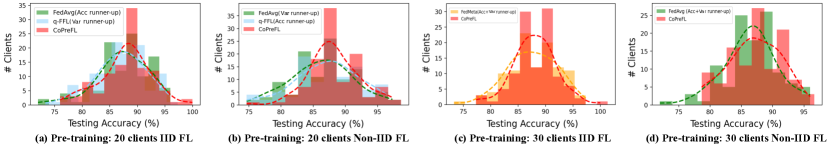
Figure 3: The distributions of testing accuracy in IID FL downstream tasks under various pre-training setups in scenario I on the CIFAR-100 dataset.

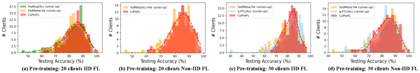
Figure 4: The distributions of testing accuracy in non-IID FL downstream tasks under various pre-training setups in scenario I on the CIFAR-100 dataset.

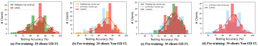
Figure 5: The distributions of testing accuracy in IID FL downstream tasks under various pre-training setups in scenario I on the Tiny-ImageNet dataset.

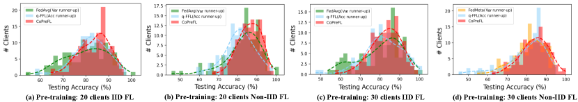
Figure 6: The distributions of testing accuracy in non-IID FL downstream tasks under various pre-training setups in scenario I on the Tiny-ImageNet dataset

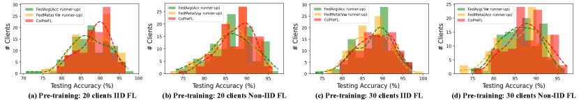
Figure 7: The distributions of testing accuracy in IID FL downstream tasks under various pre-training setups in scenario II on the CIFAR-100 dataset.

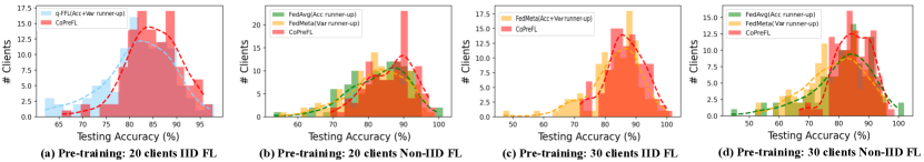
Figure 8: The distributions of testing accuracy in non-IID FL downstream tasks under various pre-training setups in scenario II on the CIFAR-100 dataset

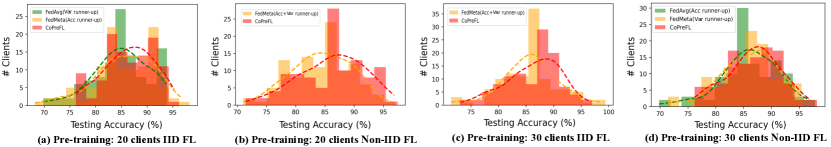
Figure 9: The distributions of testing accuracy in IID FL downstream tasks under various pre-training setups in scenario II on the Tiny-ImageNet dataset.

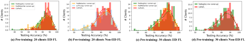
Figure 10: The distributions of testing accuracy in non-IID FL downstream tasks under various pre-training setups in scenario II on the Tiny-ImageNet dataset.

This section presents supplementary distribution results to evaluate the fairness of the pre-trained models discussed in Section 4.2. For pre-trained models trained in scenario I, Figures 3 and 4 show the testing accuracy distribution of IID and non-IID FL tasks on CIFAR-100 dataset, and Figures 5 and 6 display the respective distribution on Tiny-ImageNet dataset. Figures 7 and 8 present the testing accuracy distribution of IID and non-IID FL tasks initialized by pre-trained models trained in scenario II on CIFAR-100 dataset, and Figures 9 and 10 show the respective distribution on Tiny-ImageNet dataset. Across our experimental results, which encompass different data distribution setups and scenarios during the pre-training phase and various datasets, our CoPreFL consistently enhances the fairness of testing accuracy distributions for diverse downstream FL tasks. In general, distributions of FL tasks initialized by our CoPreFL tend to shift towards the right, indicating improved prediction performance. Moreover, when analyzing clients positioned at the left end of the distribution in each pre-training method, our approach effectively elevates underperforming clients towards the right end, resulting in enhanced predictive accuracy for these clients.

D.4 Details and Additional Results for FEMNIST Dataset

We also consider the FEMNIST dataset, widely used in FL research, following the data partition provided in (Park et al., 2021). We divide the 62 classes into 52 alphabet classes for the pre-training phase, reserving the remaining 10 digit classes for downstream FL tasks. Instead of using a ResNet-18 model, we employ a model consisting of two 3$\times$3 convolutional layers followed by two linear layers. We fixed the total number of clients as $|M|=100$ for pre-training and $|G|=10$ for downstream FL tasks. During the pre-training phase, we set the number of participants $|m|=20$ and the federated round $T=50$ for each federated pre-trained method. We use the SGD optimizer with a learning rate of $10^{-3}$ and batch size 32 for baselines and our method.

For downstream tasks, we randomly select 5 classes from a pool of 10 classes to conduct each FL task using FedAvg. We perform a total of $X=10$ FL tasks and report the average evaluations across these tasks. Each task executes FedAvg for $R=10$ rounds using the SGD optimizer with a learning rate of $10^{-3}$. Tables 41 and 42 display the averaged performance of 10 IID and 10 non-IID FL downstream tasks, initialized by various pre-training methods trained in scenario I, on the FEMNIST dataset. For scenario II, Tables 43 and 44 show the performance of IID and non-IID downstream FL tasks. The results also demonstrate that our proposed CoPreFL serves as a robust initialization for various FL setups, benefiting both performance and fairness.

D.5 Implementation Details and Additional Results for Different Initialization Methods

This section presents supplementary details and results with different initialization methods discussed in Section 4.2, including random initialization, centralized model initialization, and other FL algorithms used for initializing downstream FL. For scenario I, the centralized model is trained on a dataset collected from all $|M|=100$ clients during the pre-training phase. In scenario II, the centralized model is trained on a dataset obtained from both $|M|=100$ clients and the server. This centralized training is conducted using the SGD optimizer with a learning rate of $10^{-3}$ chosen from the range [1e-2, 5e-3, 1e-3, 5e-4], with a batch size of 64 and 50 epochs.

For FL baselines, we additionally consider SCAFFOLD (Karimireddy et al., 2019), which addresses partial client sampling, FedDyn (Acar et al., 2021), designed to tackle non-IID issues, and PerFedAvg (Fallah et al., 2020), aiming to provide an adaptable personalized model, for a detailed comparison. We train all FL algorithms for 50 rounds with $|m|=20$ participants selected from $|M|=100$ clients under a non-IID setting (Dirichlet $\alpha=0.5$) , and the final global model is used as initialization for downstream FedAvg. In the case of non-IID related FL, FedDyn, we set the parameter $\alpha$ to 0.01. For personalized FL, PerFedAvg, we employ a two-step gradient descent for local client training introduced in their paper. We use the SGD optimizer with a learning rate of $10^{-3}$, a batch size of 32, and 50 federated rounds for these FL-based baselines.

Tables 45 and 46 display the average performance of 10 FL downstream tasks initialized by different pre-training methods trained in two scenarios on the CIFAR-100 dataset and Tiny-ImageNet dataset, respectively. Comparing centralized and random initialization, we observe that the centralized method generally improves the average accuracy of downstream FL but at the cost of higher variance in most cases. However, our CoPreFL consistently enhances both average accuracy and fairness in various downstream FL tasks, demonstrating that with proper FL designs as pre-trained model, FL can be improved through initialization. Comparing with other FL designs as initialization, the results demonstrate the superiority of our method due to the considerations for unseen adaptation and performance fairness during pre-training phase.

D.6 Implementation Details and Additional Results for Different Downstream FL Tasks

In addition to the general downstream FL tasks built by FedAvg, we consider FedProx (Sahu et al., 2018) and q-FFL (Li et al., 2020), more advanced FL algorithms that addresses heterogeneity and fairness compared to FedAvg, to examine the robustness and generalizability of our pre-trained method. The experiments are conducted using the CIFAR-100 dataset under non-IID pre-training scenario I. Two additional FL algorithms, non-IID FedProx and non-IID q-FFL, are considered for downstream phase. We randomly sample 5 classes from the 20 available in our CIFAR-100 downstream dataset for each downstream task. The sampled data is then distributed to 10 clients, and the training consists of 50 rounds with 5 local iterations per round, utilizing an SGD optimizer with a learning rate of $10^{-3}$. We set the parameters $\mu=1$ for the proximal term coefficient in FedProx and $q=2$ for the loss-reweighting coefficient in q-FFL, following the optimal values reported by the authors for the CIFAR-100 dataset.

In Tables 47 and  48, the results demonstrate that our pre-trained method maintains superiority in different downstream FL algorithms compared to other pre-training methods. It is important to note that the choice of FedAvg as our downstream task is made to minimize the varying impact introduced by other FL algorithms. Comparing the pre-training $+$ downstream pairs, the improvement of CoPreFL $+$ FedAvg (in Table 1(a)) over Centralized $+$ FedProx/q-FFL (in Table 47 and  48) shows that a better initialization, which considers the distributed scenario and balances fairness/performance in the pre-training phase, could potentially benefit the inferior downstream FL algorithm.

D.7 Implementation Details when A Public Large-Scale Dataset is Available

In addition to utilizing CIFAR-100 and Tiny-ImageNet datasets, where we partition the datasets for pre-training and downstream tasks, we also explore a scenario where public large datasets are available for pre-training phase. We conducted experiments using pre-trained models with the ImageNet dataset (Deng et al., 2009), a widely used large public dataset for image classification. We sampled 200 images for each of the 1,000 classes in ImageNet_1K as a pre-training dataset. We conducted pre-training using both the centralized method and our proposed CoPreFL with ImageNet_1K. Subsequently, we conducted 10 non-IID FedAvg tasks using the CIFAR-100 dataset and initialized the models with these pre-trained models. For the centralized model in pre-training phase, we trained the model with the SGD optimizer and a learning rate of 1e-3, training the model for 50 epochs. For our proposed method during pre-training, we distributed all the sampled data across $|M|=100$ clients based on non-IID distribution (Dirichlet $\alpha=0.5$), sampling $|m|=20$ clients in each round, and conducted CoPreFL for 50 rounds. Since the goal of this experiment is to demonstrate that even with a centrally-stored public large dataset, we can intentionally distribute the dataset and apply our method, we only consider conducting our method under scenario I. For the downstream FL phase, we apply 10 IID and non-IID FedAvg tasks to the 20-class and 40-class downstream datasets we used in CIFAR-100 and Tiny-ImageNet, respectively. Each task executes FedAvg for $R=10$ rounds using the SGD optimizer with a learning rate of $10^{-3}$. Note that all classes observed during downstream tasks are the seen classes that have already appeared during pre-training, given that CIFAR-100 and Tiny-ImageNet are the subsets of ImageNet.

Table 49 shows the performance of FL downstream tasks on CIFAR-100 and Tiny-ImageNet, where the downstream tasks are initialized by different methods trained on ImageNet_1K dataset. As we can expect, models pre-trained on ImageNet_1K provide downstream FL tasks with higher accuracy compared to those pre-trained on CIFAR-100 or Tiny-ImageNet (in Table 1(a)) since there is no unseen classes when pre-trained on ImageNet. More importantly, as mentioned, we can still apply our method by intentionally splitting the dataset and mimicking the distributed nature of downstream FL to achieve further performance improvements: The centrally pre-trained model on ImageNet achieves lower accuracy and higher variance compared to our CoPreFL. This advantage of CoPreFL is achieved by initializing the model to get higher accuracy and better fairness in federated settings based on meta-learning. The overall results further confirm the advantage and applicability of our approach.

Pre-training (Scenario I, $|m|=15$)		Downstream: IID FedAvg
Distribution	Method	Acc $\uparrow$	Variance $\downarrow$	Worst 10% $\uparrow$	Worst 20% $\uparrow$	Worst 30% $\uparrow$
IID	FedAvg	87.01	15.44	78.91	80.55	81.41
	FedMeta	87.09	14.67	81.45	82.42	83.15
	q-FFL	87.25	13.25	80.85	81.52	82.26
	CoPreFL ($\gamma$ = 0.5)	87.84	11.49	82.61	83.52	84.44
Non-IID	FedAvg	85.85	15.37	78.91	80.55	81.41
	FedMeta	86.84	12.25	81.45	82.42	83.15
	q-FFL	86.37	13.54	80.85	81.52	82.26
	CoPreFL ($\gamma$ = 0.25)	86.90	8.70	81.52	82.58	83.21

Table 7: Average performance across 10 IID downstream FL tasks, initialized with various FL pre-trained methods using 15 out of 100 participants in scenario I, on the CIFAR-100 dataset.

Pre-training (Scenario I, $|m|=20$)		Downstream: IID FedAvg
Distribution	Method	Acc $\uparrow$	Variance $\downarrow$	Worst 10% $\uparrow$	Worst 20% $\uparrow$	Worst 30% $\uparrow$
IID	FedAvg	87.34	12.46	80.48	81.64	82.51
	FedMeta	86.70	14.52	81.33	82.06	82.75
	q-FFL	86.95	11.97	80.48	81.58	82.51
	CoPreFL ($\gamma$ = 0.5)	87.54	10.18	81.94	82.97	83.84
Non-IID	FedAvg	86.04	14.36	80.85	81.39	82.02
	FedMeta	86.15	16.16	79.52	81.27	82.18
	q-FFL	86.30	17.14	80.24	81.58	82.46
	CoPreFL ($\gamma$ = 0.25)	86.32	14.14	81.45	82.20	82.75

Table 8: Average performance across 10 IID downstream FL tasks, initialized with various FL pre-trained methods using 20 out of 100 participants in scenario I, on the CIFAR-100 dataset.

Pre-training (Scenario I, $|m|=25$)		Downstream: IID FedAvg
Distribution	Method	Acc $\uparrow$	Variance $\downarrow$	Worst 10% $\uparrow$	Worst 20% $\uparrow$	Worst 30% $\uparrow$
IID	FedAvg	87.68	11.36	81.58	82.79	83.68
	FedMeta	87.10	13.62	81.45	82.61	83.23
	q-FFL	87.07	17.89	80.48	81.82	82.59
	CoPreFL ($\gamma$ = 0.0)	88.13	9.30	82.85	83.94	84.75
Non-IID	FedAvg	86.78	11.90	81.09	81.82	82.55
	FedMeta	85.41	15.05	79.15	79.94	80.81
	q-FFL	85.92	12.11	79.03	80.55	81.49
	CoPreFL ($\gamma$ = 0.0)	86.84	11.16	82.06	82.85	83.43

Table 9: Average performance across 10 IID downstream FL tasks, initialized with various FL pre-trained methods using 25 out of 100 participants in scenario I, on the CIFAR-100 dataset.

Pre-training (Scenario I, $|m|=30$)		Downstream: IID FedAvg
Distribution	Method	Acc $\uparrow$	Variance $\downarrow$	Worst 10% $\uparrow$	Worst 20% $\uparrow$	Worst 30%
IID	FedAvg	86.52	13.54	80.85	81.76	82.55
	FedMeta	87.65	13.47	81.58	82.91	83.64
	q-FFL	86.40	15.68	79.27	80.12	81.45
	CoPreFL ($\gamma$ = 0.0 )	87.90	11.16	82.67	83.58	84.36
Non-IID	FedAvg	86.78	12.32	80.85	81.76	82.55
	FedMeta	85.87	17.22	81.58	82.09	82.64
	q-FFL	85.77	13.40	79.27	80.12	81.45
	CoPreFL ($\gamma$ = 0.5)	87.04	9.18	81.70	82.12	82.91

Table 10: Average performance across 10 IID downstream FL tasks, initialized with various FL pre-trained methods using 30 out of 100 participants in scenario I, on the CIFAR-100 dataset.

Pre-training (Scenario I, $|m|=15$)		Downstream: Non-IID FedAvg
Distribution	Method	Acc $\uparrow$	Variance $\downarrow$	Worst 10% $\uparrow$	Worst 20% $\uparrow$	Worst 30% $\uparrow$
IID	FedAvg	81.46	62.09	68.87	71.12	72.76
	FedMeta	81.20	63.84	69.39	71.52	73.14
	q-FFL	83.45	39.94	69.95	73.66	75.43
	CoPreFL ($\gamma$ = 0.75)	84.79	37.09	72.71	74.80	76.75
Non-IID	FedAvg	83.76	51.84	69.50	72.80	74.30
	FedMeta	82.65	39.19	69.39	72.76	74.87
	q-FFL	82.00	53.00	70.78	73.03	74.22
	CoPreFL ($\gamma$ = 0.25)	84.55	38.07	71.47	73.40	75.20

Table 11: Average performance across 10 non-IID downstream FL tasks, initialized with various FL pre-trained methods using 15 out of 100 participants in scenario I, on the CIFAR-100 dataset.

Pre-training (Scenario I, $|m|=20$)		Downstream: Non-IID FedAvg
Distribution	Method	Acc $\uparrow$	Variance $\downarrow$	Worst 10% $\uparrow$	Worst 20% $\uparrow$	Worst 30% $\uparrow$
IID	FedAvg	84.20	57.15	68.43	71.83	74.38
	FedMeta	83.80	42.64	72.30	73.79	75.47
	q-FFL	82.60	45.56	70.46	73.41	75.14
	CoPreFL ($\gamma$ = 0.25)	84.36	38.56	73.66	75.63	77.40
Non-IID	FedAvg	78.96	64.80	62.70	67.00	69.80
	FedMeta	82.45	48.72	68.97	72.41	74.35
	q-FFL	80.01	88.92	64.39	67.48	70.30
	CoPreFL ($\gamma$ = 0.75)	83.29	34.69	71.58	73.20	74.59

Table 12: Average performance across 10 non-IID downstream FL tasks, initialized with various FL pre-trained methods using 20 out of 100 participants in scenario I, on the CIFAR-100 dataset.

Pre-training (Scenario I, $|m|=25$)		Downstream: Non-IID FedAvg
Distribution	Method	Acc $\uparrow$	Variance $\downarrow$	Worst 10% $\uparrow$	Worst 20% $\uparrow$	Worst 30% $\uparrow$
IID	FedAvg	84.02	51.98	71.26	73.21	75.57
	FedMeta	82.44	55.06	68.53	71.73	73.95
	q-FFL	82.63	47.20	70.52	72.42	74.01
	CoPreFL ($\gamma$ = 0.75)	85.60	37.45	74.42	76.53	78.43
Non-IID	FedAvg	82.01	39.82	70.75	73.02	74.63
	FedMeta	84.02	39.56	71.86	75.17	76.80
	q-FFL	82.18	46.79	70.53	72.43	73.61
	CoPreFL ($\gamma$ = 0.25)	85.72	29.38	75.81	77.24	78.54

Table 13: Average performance across 10 non-IID downstream FL tasks, initialized with various FL pre-trained methods using 25 out of 100 participants in scenario I, on the CIFAR-100 dataset.

Pre-training (Scenario I, $|m|=30$)		Downstream: Non-IID FedAvg
Distribution	Method	Acc $\uparrow$	Variance $\downarrow$	Worst 10% $\uparrow$	Worst 20% $\uparrow$	Worst 30% $\uparrow$
IID	FedAvg	79.60	83.36	62.68	65.87	68.57
	FedMeta	79.90	48.02	67.01	69.69	71.46
	q-FFL	83.02	52.27	70.64	72.71	74.50
	CoPreFL ($\gamma$ = 0.75)	83.48	45.16	70.80	72.72	74.59
Non-IID	FedAvg	81.79	50.84	69.70	72.08	74.20
	FedMeta	82.61	43.43	71.84	73.30	74.68
	q-FFL	82.68	54.17	68.68	72.08	74.06
	CoPreFL ($\gamma$ = 0.75)	83.48	40.20	72.83	74.29	75.80

Table 14: Average performance across 10 non-IID downstream FL tasks, initialized with various FL pre-trained methods using 30 out of 100 participants in scenario I, on the CIFAR-100 dataset.

Pre-training (Scenario I, $|m|=15$)		Downstream: IID FedAvg
Distribution	Method	Acc $\uparrow$	Variance $\downarrow$	Worst 10% $\uparrow$	Worst 20% $\uparrow$	Worst 30% $\uparrow$
IID	FedAvg	84.27	16.48	77.20	78.43	79.27
	FedMeta	84.15	19.27	78.50	79.65	80.66
	q-FFL	84.24	17.64	77.20	78.86	79.99
	CoPreFL ($\gamma$ = 0.0)	85.05	15.21	79.08	80.38	81.19
Non-IID	FedAvg	85.19	15.13	77.78	79.29	80.38
	FedMeta	85.35	15.60	78.50	80.01	81.00
	q-FFL	85.91	15.76	78.22	80.38	81.12
	CoPreFL ($\gamma$ = 0.0)	86.39	10.63	79.08	80.45	81.24

Table 15: Average performance across 10 IID downstream FL tasks, initialized with various FL pre-trained methods using 15 out of 100 participants in scenario I, on the Tiny-ImageNet dataset.

Pre-training (Scenario I, $|m|=20$)		Downstream: IID FedAvg
Distribution	Method	Acc $\uparrow$	Variance $\downarrow$	Worst 10% $\uparrow$	Worst 20% $\uparrow$	Worst 30% $\uparrow$
IID	FedAvg	85.74	17.39	77.20	78.79	79.80
	FedMeta	85.56	17.64	77.92	79.51	80.57
	q-FFL	84.64	21.07	78.79	79.74	80.91
	CoPreFL ($\gamma$ = 0.5)	86.03	13.99	79.08	80.09	81.24
Non-IID	FedAvg	85.43	17.31	77.49	79.65	80.76
	FedMeta	84.16	16.89	77.20	79.73	81.05
	q-FFL	85.83	19.18	78.07	79.37	80.62
	CoPreFL ($\gamma$ = 0.5)	86.00	16.16	79.37	80.30	81.19

Table 16: Average performance across 10 IID downstream FL tasks, initialized with various FL pre-trained methods using 20 out of 100 participants in scenario I, on the Tiny-ImageNet dataset.

Pre-training (Scenario I, $|m|=25$)		Downstream: IID FedAvg
Distribution	Method	Acc $\uparrow$	Variance $\downarrow$	Worst 10% $\uparrow$	Worst 20% $\uparrow$	Worst 30% $\uparrow$
IID	FedAvg	85.24	19.71	78.35	79.87	81.05
	FedMeta	85.19	22.00	78.21	79.73	80.71
	q-FFL	85.26	16.89	78.50	79.94	81.00
	CoPreFL ($\gamma$ = 0.75)	85.74	12.81	79.84	80.68	81.49
Non-IID	FedAvg	85.47	14.36	77.63	79.29	80.33
	FedMeta	85.74	17.64	77.92	79.80	81.10
	q-FFL	85.82	17.64	79.08	80.52	81.58
	CoPreFL ($\gamma$ = 0.0)	86.25	12.96	79.87	80.99	81.68

Table 17: Average performance across 10 IID downstream FL tasks, initialized with various FL pre-trained methods using 25 out of 100 participants in scenario I, on the Tiny-ImageNet dataset.

Pre-training (Scenario I, $|m|=30$)		Downstream: IID FedAvg
Distribution	Method	Acc $\uparrow$	Variance $\downarrow$	Worst 10% $\uparrow$	Worst 20% $\uparrow$	Worst 30% $\uparrow$
IID	FedAvg	85.71	14.90	79.08	80.66	81.53
	FedMeta	85.48	15.92	79.51	80.16	81.19
	q-FFL	85.95	21.25	77.34	78.93	80.13
	CoPreFL ($\gamma$ = 0.75)	86.05	14.90	80.31	81.49	82.27
Non-IID	FedAvg	85.64	21.07	75.90	77.99	79.32
	FedMeta	85.90	17.89	80.23	81.10	81.87
	q-FFL	86.49	14.75	78.79	80.16	81.24
	CoPreFL ($\gamma$ = 0.0)	86.51	14.06	80.74	81.35	82.16

Table 18: Average performance across 10 IID downstream FL tasks, initialized with various FL pre-trained methods using 30 out of 100 participants in scenario I, on the Tiny-ImageNet dataset.

Pre-training (Scenario I, $|m|=15$)		Downstream: Non-IID FedAvg
Distribution	Method	Acc $\uparrow$	Variance $\downarrow$	Worst 10% $\uparrow$	Worst 20% $\uparrow$	Worst 30% $\uparrow$
IID	FedAvg	78.88	64.16	67.03	68.42	69.95
	FedMeta	82.62	43.16	70.76	73.48	74.48
	q-FFL	83.58	49.70	67.11	71.38	73.78
	CoPreFL ($\gamma$ = 0.5)	83.83	41.22	73.28	74.39	75.50
Non-IID	FedAvg	82.19	38.32	72.64	73.90	75.38
	FedMeta	81.45	53.73	68.42	71.17	72.98
	q-FFL	82.85	32.26	73.89	76.14	77.28
	CoPreFL ($\gamma$ = 0.25)	83.65	25.81	75.41	76.45	77.73

Table 19: Average performance across 10 non-IID downstream FL tasks, initialized with various FL pre-trained methods using 15 out of 100 participants in scenario I, on the Tiny-ImageNet dataset.

Pre-training (Scenario I, $|m|=20$)		Downstream: Non-IID FedAvg
Distribution	Method	Acc $\uparrow$	Variance $\downarrow$	Worst 10% $\uparrow$	Worst 20% $\uparrow$	Worst 30% $\uparrow$
IID	FedAvg	79.45	35.40	64.86	68.61	70.78
	FedMeta	81.68	65.61	65.96	69.17	71.59
	q-FFL	82.65	39.69	70.65	74.14	76.27
	CoPreFL ($\gamma$ = 0.0)	83.79	34.93	72.59	75.05	76.76
Non-IID	FedAvg	82.94	37.21	68.99	72.29	74.40
	FedMeta	81.03	37.58	69.44	71.55	72.93
	q-FFL	84.11	43.96	73.87	76.05	77.37
	CoPreFL ($\gamma$ = 0.5)	85.23	35.40	76.77	78.46	79.86

Table 20: Average performance across 10 non-IID downstream FL tasks, initialized with various FL pre-trained methods using 20 out of 100 participants in scenario I, on the Tiny-ImageNet dataset.

Pre-training (Scenario I, $|m|=25$)		Downstream: Non-IID FedAvg
Distribution	Method	Acc $\uparrow$	Variance $\downarrow$	Worst 10% $\uparrow$	Worst 20% $\uparrow$	Worst 30% $\uparrow$
IID	FedAvg	83.71	50.41	69.91	73.50	75.40
	FedMeta	84.19	42.90	73.77	76.22	77.77
	q-FFL	80.11	55.20	65.45	68.54	70.72
	CoPreFL ($\gamma$ = 0.0)	84.29	36.60	76.02	77.56	78.95
Non-IID	FedAvg	79.08	55.80	66.80	69.06	71.38
	FedMeta	81.58	38.07	70.86	72.83	74.39
	q-FFL	83.16	45.56	72.39	75.29	77.09
	CoPreFL ($\gamma$ = 0.25)	83.87	25.60	75.16	76.87	78.05

Table 21: Average performance across 10 non-IID downstream FL tasks, initialized with various FL pre-trained methods using 25 out of 100 participants in scenario I, on the Tiny-ImageNet dataset.

Pre-training (Scenario I, $|m|=30$)		Downstream: Non-IID FedAvg
Distribution	Method	Acc $\uparrow$	Variance $\downarrow$	Worst 10% $\uparrow$	Worst 20% $\uparrow$	Worst 30% $\uparrow$
IID	FedAvg	80.37	43.56	69.27	70.91	72.44
	FedMeta	80.51	44.09	68.05	70.74	72.18
	q-FFL	81.89	45.97	68.85	72.07	73.99
	CoPreFL ($\gamma$ = 0.0)	83.17	31.81	71.16	73.64	75.49
Non-IID	FedAvg	82.73	42.51	72.90	74.84	76.50
	FedMeta	82.58	34.81	71.67	74.39	75.85
	q-FFL	83.39	38.07	72.60	74.97	76.57
	CoPreFL ($\gamma$ = 0.75)	84.25	30.11	76.18	77.54	78.73

Table 22: Average performance across 10 non-IID downstream FL tasks, initialized with various FL pre-trained methods using 30 out of 100 participants in scenario I, on the Tiny-ImageNet dataset.

Pre-training (Scenario I, $|m|=20$)	Downstream: Non-IID FedAvg
Method	Acc $\uparrow$	Variance $\downarrow$	Worst 10% $\uparrow$	Worst 20% $\uparrow$	Worst 30% $\uparrow$
FedAvg	81.35	59.69	70.35	70.91	71.63
FedMeta	82.69	46.38	72.74	73.51	74.39
q-FFL	83.27	51.48	73.01	73.82	75.02
CoPreFL ($\gamma$ = 0.5)	84.71	39.26	73.28	74.99	75.35

Table 23: Performance of 20-way classification downstream FedAvg, initialized with various non-IID FL pre-trained methods in scenario I, on the CIFAR-100 dataset.

Pre-training (Scenario II, $|m|=15$)		Downstream: IID FedAvg
Distribution	Method	Acc $\uparrow$	Variance $\downarrow$	Worst 10% $\uparrow$	Worst 20% $\uparrow$	Worst 30% $\uparrow$
IID	FedAvg	87.02	12.82	82.42	83.33	84.04
	FedMeta	87.07	10.76	81.94	82.73	83.43
	q-FFL	87.27	13.69	81.21	82.30	82.95
	CoPreFL-SGD ($\gamma$ = 0.25)	87.87	13.32	82.73	83.58	84.06
	CoPreFL ($\gamma$ = 0.25)	88.58	8.70	83.39	83.88	84.69
Non-IID	FedAvg	86.22	15.44	79.15	80.36	81.54
	FedMeta	86.09	11.42	80.12	81.03	81.98
	q-FFL	86.56	15.29	78.42	80.00	81.37
	CoPreFL-SGD ($\gamma$ = 0.75)	86.73	12.46	80.61	81.76	82.63
	CoPreFL ($\gamma$ = 0.75)	87.42	9.06	81.21	82.30	82.95

Table 24: Average performance across 10 IID downstream FL tasks, initialized with various FL pre-trained methods using 15 out of 100 participants in scenario II, on the CIFAR-100 dataset.

Pre-training (Scenario II, $|m|=20$)		Downstream: IID FedAvg
Distribution	Method	Acc $\uparrow$	Variance $\downarrow$	Worst 10% $\uparrow$	Worst 20% $\uparrow$	Worst 30% $\uparrow$
IID	FedAvg	87.28	15.21	80.00	81.21	82.10
	FedMeta	87.27	12.46	81.45	82.12	82.95
	q-FFL	86.84	12.74	80.73	82.12	82.87
	CoPreFL-SGD ($\gamma$ = 0.5)	87.67	12.32	81.82	83.09	83.92
	CoPreFL ($\gamma$ = 0.5)	88.10	9.30	83.52	84.30	85.05
Non-IID	FedAvg	86.39	17.31	79.64	80.79	81.78
	FedMeta	86.32	12.46	80.61	81.45	82.26
	q-FFL	86.17	16.24	79.27	81.09	82.02
	CoPreFL-SGD ($\gamma$ = 0.25)	86.63	11.76	81.21	82.00	82.46
	CoPreFL ($\gamma$ = 0.25)	87.02	10.50	81.70	82.42	83.23

Table 25: Average performance across 10 IID downstream FL tasks, initialized with various FL pre-trained methods using 20 out of 100 participants in scenario II, on the CIFAR-100 dataset.

Pre-training (Scenario II, $|m|=25$)		Downstream: IID FedAvg
Distribution	Method	Acc $\uparrow$	Variance $\downarrow$	Worst 10% $\uparrow$	Worst 20% $\uparrow$	Worst 30% $\uparrow$
IID	FedAvg	87.31	14.90	79.39	81.64	82.75
	FedMeta	86.81	10.89	80.97	82.30	83.07
	q-FFL	87.36	17.47	80.73	81.76	82.87
	CoPreFL-SGD ($\gamma$ = 0.5)	87.98	11.22	82.55	83.15	83.92
	CoPreFL ($\gamma$ = 0.5)	88.67	9.98	83.88	84.55	85.29
Non-IID	FedAvg	86.37	15.44	78.79	80.12	81.25
	FedMeta	85.49	16.89	79.27	80.36	81.25
	q-FFL	85.67	17.06	80.61	81.45	81.98
	CoPreFL-SGD ($\gamma$ = 0.75)	86.40	13.10	80.62	81.45	82.34
	CoPreFL ($\gamma$ = 0.75)	87.32	11.22	82.42	83.27	83.84

Table 26: Average performance across 10 IID downstream FL tasks, initialized with various FL pre-trained methods using 25 out of 100 participants in scenario II, on the CIFAR-100 dataset.

Pre-training (Scenario II, $|m|=30$)		Downstream: IID FedAvg
Distribution	Method	Acc $\uparrow$	Variance $\downarrow$	Worst 10% $\uparrow$	Worst 20% $\uparrow$	Worst 30% $\uparrow$
IID	FedAvg	87.51	13.76	82.55	83.58	84.20
	FedMeta	87.25	12.39	81.70	82.55	83.03
	q-FFL	86.78	13.76	81.21	82.06	82.79
	CoPreFL-SGD ($\gamma$ = 0.75)	87.75	13.40	81.52	82.94	83.70
	CoPreFL ($\gamma$ = 0.75)	88.27	9.06	84.06	84.55	85.05
Non-IID	FedAvg	86.07	11.09	80.61	81.64	82.38
	FedMeta	86.25	12.96	79.03	80.36	81.66
	q-FFL	85.50	15.29	77.58	79.39	80.57
	CoPreFL-SGD ($\gamma$ = 0.5)	86.47	10.96	80.36	81.36	82.00
	CoPreFL ($\gamma$ = 0.5)	87.54	10.96	81.09	81.67	82.40

Table 27: Average performance across 10 IID downstream FL tasks, initialized with various FL pre-trained methods using 30 out of 100 participants in scenario II, on the CIFAR-100 dataset.

Pre-training (Scenario II, $|m|=15$)		Downstream: Non-IID FedAvg
Distribution	Method	Acc $\uparrow$	Variance $\downarrow$	Worst 10% $\uparrow$	Worst 20% $\uparrow$	Worst 30% $\uparrow$
IID	FedAvg	84.02	46.79	71.01	74.53	76.81
	FedMeta	83.47	34.11	73.68	75.20	76.35
	q-FFL	85.03	35.64	74.04	76.39	78.12
	CoPreFL-SGD ($\gamma$ = 0.75)	85.04	35.64	74.61	76.40	78.34
	CoPreFL ($\gamma$ = 0.75)	85.08	31.70	74.61	76.87	78.63
Non-IID	FedAvg	82.91	41.99	71.90	75.23	76.81
	FedMeta	78.77	70.39	65.13	67.47	69.28
	q-FFL	80.94	49.42	69.57	71.46	72.86
	CoPreFL-SGD ($\gamma$ = 0.25)	83.42	40.20	73.09	74.54	76.29
	CoPreFL ($\gamma$ = 0.25)	83.83	39.31	74.26	76.42	78.10

Table 28: Average performance across 10 non-IID downstream FL tasks, initialized with various FL pre-trained methods using 15 out of 100 participants in scenario II, on the CIFAR-100 dataset.

Pre-training (Scenario II, $|m|=20$)		Downstream: Non-IID FedAvg
Distribution	Method	Acc $\uparrow$	Variance $\downarrow$	Worst 10% $\uparrow$	Worst 20% $\uparrow$	Worst 30% $\uparrow$
IID	FedAvg	81.79	41.73	69.84	73.47	75.11
	FedMeta	82.29	47.75	71.69	74.17	75.71
	q-FFL	82.40	40.32	73.96	75.30	76.59
	CoPreFL-SGD ($\gamma$ = 0.75)	82.90	38.94	73.02	75.60	77.18
	CoPreFL ($\gamma$ = 0.75)	85.68	27.14	75.36	77.25	78.49
Non-IID	FedAvg	82.82	49.00	69.71	72.54	74.58
	FedMeta	82.69	48.44	68.84	71.82	74.14
	q-FFL	82.14	73.10	68.22	70.64	73.77
	CoPreFL-SGD ($\gamma$ = 0.25)	83.63	41.73	69.76	73.46	75.64
	CoPreFL ($\gamma$ = 0.25)	86.63	31.58	73.05	75.82	77.58

Table 29: Average performance across 10 non-IID downstream FL tasks, initialized with various FL pre-trained methods using 20 out of 100 participants in scenario II, on the CIFAR-100 dataset.

Pre-training (Scenario II, $|m|=25$)		Downstream: Non-IID FedAvg
Distribution	Method	Acc $\uparrow$	Variance $\downarrow$	Worst 10% $\uparrow$	Worst 20% $\uparrow$	Worst 30% $\uparrow$
IID	FedAvg	80.53	62.57	66.51	68.54	70.78
	FedMeta	82.37	45.97	70.68	73.40	75.21
	q-FFL	82.06	48.44	71.08	73.03	74.71
	CoPreFL-SGD ($\gamma$ = 0.25)	82.62	75.86	68.12	70.73	72.51
	CoPreFL ($\gamma$ = 0.25)	85.05	33.99	75.12	76.74	77.79
Non-IID	FedAvg	84.06	40.07	71.11	73.36	75.67
	FedMeta	81.40	47.33	67.41	70.87	72.49
	q-FFL	82.30	55.06	67.82	71.53	73.70
	CoPreFL-SGD ($\gamma$ = 0.5)	84.25	53.88	71.62	73.48	75.92
	CoPreFL ($\gamma$ = 0.5)	84.92	39.82	75.04	77.45	78.93

Table 30: Average performance across 10 non-IID downstream FL tasks, initialized with various FL pre-trained methods using 25 out of 100 participants in scenario II, on the CIFAR-100 dataset.

Pre-training (Scenario II, $|m|=30$)		Downstream: Non-IID FedAvg
Distribution	Method	Acc $\uparrow$	Variance $\downarrow$	Worst 10% $\uparrow$	Worst 20% $\uparrow$	Worst 30% $\uparrow$
IID	FedAvg	82.70	62.09	66.99	71.18	73.18
	FedMeta	83.00	39.94	71.16	73.43	75.52
	q-FFL	82.81	44.09	71.82	73.68	75.31
	CoPreFL-SGD ($\gamma$ = 0.25)	85.05	37.33	75.16	76.79	78.21
	CoPreFL ($\gamma$ = 0.25)	85.78	35.88	75.26	78.60	80.55
Non-IID	FedAvg	81.14	71.23	65.42	69.17	70.99
	FedMeta	78.98	64.48	63.97	66.89	69.06
	q-FFL	79.87	70.06	63.96	67.47	70.16
	CoPreFL-SGD ($\gamma$ = 0.75)	83.21	37.94	72.75	74.53	76.01
	CoPreFL ($\gamma$ = 0.75)	85.11	36.84	72.66	75.63	77.47

Table 31: Average performance across 10 non-IID downstream FL tasks, initialized with various FL pre-trained methods using 30 out of 100 participants in scenario II, on the CIFAR-100 dataset.

Pre-training (Scenario II, $|m|=15$)		Downstream: IID FedAvg
Distribution	Method	Acc $\uparrow$	Variance $\downarrow$	Worst 10% $\uparrow$	Worst 20% $\uparrow$	Worst 30% $\uparrow$
IID	FedAvg	85.79	16.16	77.34	78.37	80.17
	FedMeta	85.88	17.47	77.49	78.93	80.33
	q-FFL	85.24	15.60	77.38	78.37	80.23
	CoPreFL-SGD ($\gamma$ = 0.75)	85.37	14.82	77.49	79.00	80.33
	CoPreFL ($\gamma$ = 0.75)	86.64	14.59	80.23	81.17	82.06
Non-IID	FedAvg	85.17	16.56	78.21	79.73	80.52
	FedMeta	85.76	18.40	78.93	80.52	81.39
	q-FFL	86.29	18.06	78.79	80.38	81.58
	CoPreFL-SGD ($\gamma$ = 0.25)	85.49	13.84	79.65	80.66	82.07
	CoPreFL ($\gamma$ = 0.25)	86.68	12.67	80.09	81.02	82.36

Table 32: Average performance across 10 IID downstream FL tasks, initialized with various FL pre-trained methods using 15 out of 100 participants in scenario II, on the Tiny-ImageNet dataset.

Pre-training (Scenario II, $|m|=20$)		Downstream: IID FedAvg
Distribution	Method	Acc $\uparrow$	Variance $\downarrow$	Worst 10% $\uparrow$	Worst 20% $\uparrow$	Worst 30% $\uparrow$
IID	FedAvg	85.08	14.29	78.21	79.44	80.52
	FedMeta	85.39	19.89	78.33	79.30	80.48
	q-FFL	85.41	20.70	77.63	79.22	80.28
	CoPreFL-SGD ($\gamma$ = 0.75)	85.57	17.89	78.64	80.01	80.95
	CoPreFL ($\gamma$ = 0.75)	86.77	12.25	80.52	81.17	81.96
Non-IID	FedAvg	85.15	20.98	79.04	80.45	81.34
	FedMeta	85.38	14.82	78.79	80.59	81.58
	q-FFL	85.46	19.71	78.81	80.11	81.97
	CoPreFL-SGD ($\gamma$ = 0.75)	85.57	18.75	79.65	81.10	82.06
	CoPreFL ($\gamma$ = 0.75)	86.74	12.82	80.66	81.60	82.49

Table 33: Average performance across 10 IID downstream FL tasks, initialized with various FL pre-trained methods using 20 out of 100 participants in scenario II, on the Tiny-ImageNet dataset.

Pre-training (Scenario II, $|m|=25$)		Downstream: IID FedAvg
Distribution	Method	Acc $\uparrow$	Variance $\downarrow$	Worst 10% $\uparrow$	Worst 20% $\uparrow$	Worst 30% $\uparrow$
IID	FedAvg	85.99	16.65	78.50	79.73	80.66
	FedMeta	85.58	19.89	78.21	79.80	80.81
	q-FFL	85.66	17.22	78.07	79.73	80.71
	CoPreFL-SGD ($\gamma$ = 0.5)	86.33	15.44	80.63	81.35	82.28
	CoPreFL ($\gamma$ = 0.5)	86.72	15.29	80.94	81.59	82.20
Non-IID	FedAvg	85.50	16.48	78.35	79.80	80.86
	FedMeta	86.57	17.81	78.93	79.80	80.86
	q-FFL	86.45	14.82	79.08	80.74	81.96
	CoPreFL-SGD ($\gamma$ = 0.5)	86.61	13.62	79.37	80.45	81.19
	CoPreFL ($\gamma$ = 0.5)	87.16	10.43	80.38	81.39	82.20

Table 34: Average performance across 10 IID downstream FL tasks, initialized with various FL pre-trained methods using 25 out of 100 participants in scenario II, on the Tiny-ImageNet dataset.

Pre-training (Scenario II, $|m|=30$)		Downstream: IID FedAvg
Distribution	Method	Acc $\uparrow$	Variance $\downarrow$	Worst 10% $\uparrow$	Worst 20% $\uparrow$	Worst 30% $\uparrow$
IID	FedAvg	85.27	14.90	77.92	79.15	80.04
	FedMeta	85.61	13.54	78.07	79.87	81.14
	q-FFL	85.34	17.22	80.37	81.39	82.15
	CoPreFL-SGD ($\gamma$ = 1.0)	85.61	12.25	79.94	80.74	81.29
	CoPreFL ($\gamma$ = 1.0)	86.62	11.69	81.24	81.89	82.64
Non-IID	FedAvg	85.70	20.61	78.64	80.09	81.19
	FedMeta	85.44	16.56	79.08	80.38	81.34
	q-FFL	85.54	17.56	79.22	80.66	81.67
	CoPreFL-SGD ($\gamma$ = 0.5)	85.79	14.21	79.65	80.59	81.43
	CoPreFL ($\gamma$ = 0.5)	86.15	13.25	80.66	81.89	82.68

Table 35: Average performance across 10 IID downstream FL tasks, initialized with various FL pre-trained methods using 30 out of 100 participants in scenario II, on the Tiny-ImageNet dataset.

Pre-training (Scenario II, $|m|=15$)		Downstream: Non-IID FedAvg
Distribution	Method	Acc $\uparrow$	Variance $\downarrow$	Worst 10% $\uparrow$	Worst 20% $\uparrow$	Worst 30% $\uparrow$
IID	FedAvg	82.50	39.06	70.33	73.19	75.15
	FedMeta	81.57	62.57	67.65	70.95	72.83
	q-FFL	82.31	48.16	70.00	72.07	73.99
	CoPreFL-SGD ($\gamma$ = 0.75)	83.11	38.94	72.06	73.63	75.29
	CoPreFL ($\gamma$ = 0.75)	84.68	33.76	73.84	75.50	77.35
Non-IID	FedAvg	80.19	53.00	67.13	69.67	71.36
	FedMeta	81.94	56.40	67.15	71.39	73.39
	q-FFL	81.64	54.46	69.58	71.65	73.02
	CoPreFL-SGD ($\gamma$ = 0.25)	83.57	41.22	71.46	73.45	75.41
	CoPreFL ($\gamma$ = 0.25)	84.26	28.52	73.61	75.55	76.79

Table 36: Average performance across 10 non-IID downstream FL tasks, initialized with various FL pre-trained methods using 15 out of 100 participants in scenario II, on the Tiny-ImageNet dataset.

Pre-training (Scenario II, $|m|=20$)		Downstream: Non-IID FedAvg
Distribution	Method	Acc $\uparrow$	Variance $\downarrow$	Worst 10% $\uparrow$	Worst 20% $\uparrow$	Worst 30% $\uparrow$
IID	FedAvg	81.91	77.97	64.37	71.67	74.51
	FedMeta	81.58	38.56	70.94	71.82	73.09
	q-FFL	82.17	48.58	70.22	72.66	74.24
	CoPreFL-SGD ($\gamma$ = 0.5)	82.32	42.25	71.61	73.31	74.62
	CoPreFL ($\gamma$ = 0.5)	84.48	35.64	73.66	74.75	76.21
Non-IID	FedAvg	82.87	48.16	68.94	72.91	75.28
	FedMeta	84.19	49.70	70.41	72.63	74.74
	q-FFL	83.51	44.22	69.91	73.71	76.01
	CoPreFL-SGD ($\gamma$ = 0.5)	84.30	36.24	72.83	75.64	77.37
	CoPreFL ($\gamma$ = 0.5)	84.72	24.80	75.84	77.31	78.50

Table 37: Average performance across 10 non-IID downstream FL tasks, initialized with various FL pre-trained methods using 20 out of 100 participants in scenario II, on the Tiny-ImageNet dataset.

Pre-training (Scenario II, $|m|=25$)		Downstream: Non-IID FedAvg
Distribution	Method	Acc $\uparrow$	Variance $\downarrow$	Worst 10% $\uparrow$	Worst 20% $\uparrow$	Worst 30% $\uparrow$
IID	FedAvg	83.42	44.36	70.04	72.88	75.10
	FedMeta	80.66	45.29	68.38	70.89	73.05
	q-FFL	83.60	34.93	74.41	75.86	77.29
	CoPreFL-SGD ($\gamma$ = 0.75)	84.49	46.51	72.66	74.48	75.97
	CoPreFL ($\gamma$ = 0.75)	84.81	32.15	76.65	77.97	79.12
Non-IID	FedAvg	79.44	64.80	65.35	68.25	70.19
	FedMeta	81.22	48.58	69.53	71.87	73.52
	q-FFL	82.14	41.60	72.32	74.56	76.31
	CoPreFL-SGD ($\gamma$ = 0.5)	82.88	35.64	71.25	73.00	74.32
	CoPreFL ($\gamma$ = 0.5)	84.02	24.01	75.49	77.02	78.17

Table 38: Average performance across 10 non-IID downstream FL tasks, initialized with various FL pre-trained methods using 25 out of 100 participants in scenario II, on the Tiny-ImageNet dataset.

Pre-training (Scenario II, $|m|=30$)		Downstream: Non-IID FedAvg
Distribution	Method	Acc $\uparrow$	Variance $\downarrow$	Worst 10% $\uparrow$	Worst 20% $\uparrow$	Worst 30% $\uparrow$
IID	FedAvg	83.63	42.25	71.27	73.56	75.00
	FedMeta	83.41	39.82	72.34	72.81	73.15
	q-FFL	82.98	63.68	62.50	65.62	68.31
	CoPreFL-SGD ($\gamma$ = 0.25)	83.66	42.90	71.84	74.30	75.70
	CoPreFL ($\gamma$ = 0.25)	84.26	39.31	73.77	75.91	77.58
Non-IID	FedAvg	83.24	42.25	69.06	73.39	75.31
	FedMeta	81.61	47.89	69.38	72.47	74.39
	q-FFL	81.92	51.55	69.73	72.17	74.38
	CoPreFL-SGD ($\gamma$ = 0.0)	83.37	46.38	72.17	74.15	75.53
	CoPreFL ($\gamma$ = 0.0)	85.45	38.32	74.43	75.90	77.45

Table 39: Average performance across 10 non-IID downstream FL tasks, initialized with various FL pre-trained methods using 30 out of 100 participants in scenario II, on the Tiny-ImageNet dataset.

Pre-training (Scenario II)	Downstream: Non-IID FedAvg
Method	Acc $\uparrow$	Variance $\downarrow$	Worst 10% $\uparrow$	Worst 20% $\uparrow$	Worst 30% $\uparrow$
FedAvg	83.15	51.19	70.33	72.17	73.49
FedMeta	81.77	39.52	69.71	71.55	73.68
q-FFL	83.39	51.77	70.63	72.91	74.28
CoPreFL-SGD ($\gamma$ = 0.25)	83.63	41.73	69.76	73.46	75.64
CoPreFL ($\gamma$ = 0.25)	86.63	31.58	73.05	75.82	77.58

Table 40: Average performance across 10 non-IID downstream FL tasks, initialized with various non-IID FL pre-trained models. Note that, for FedAvg, FedMeta, and q-FFL baselines, the dataset is distributed from all clients’ and server’s data without a further refining step, while our method is trained on clients’ data and refined using the server’s dataset.

Pre-training (Scenario I, $|m|=20$)		Downstream: IID FedAvg
Distribution	Method	Acc $\uparrow$	Variance $\downarrow$	Worst 10% $\uparrow$	Worst 20% $\uparrow$	Worst 30% $\uparrow$
IID	FedAvg	86.84	2.43	76.88	79.87	81.47
	FedMeta	82.16	2.31	75.32	75.97	76.62
	q-FFL	79.91	3.09	76.62	77.40	77.83
	CoPreFL ($\gamma$ = 0.75)	91.59	1.61	86.75	87.40	88.31
Non-IID	FedAvg	83.84	2.13	75.97	77.88	80.79
	FedMeta	86.71	1.61	74.69	77.82	78.21
	q-FFL	79.85	2.53	69.22	71.95	74.94
	CoPreFL ($\gamma$ = 0.5)	89.01	1.46	81.29	83.55	84.24

Table 41: Average performance across 10 IID downstream FL tasks, initialized with various FL pre-trained methods using 20 out of 100 participants in scenario I, on the FEMNIST dataset.

Pre-training (Scenario I, $|m|=20$)		Downstream: Non-IID FedAvg
Distribution	Method	Acc $\uparrow$	Variance $\downarrow$	Worst 10% $\uparrow$	Worst 20% $\uparrow$	Worst 30% $\uparrow$
IID	FedAvg	75.04	16.16	70.75	71.65	72.19
	FedMeta	69.61	6.81	59.19	62.35	64.54
	q-FFL	70.47	19.30	58.31	61.66	63.67
	CoPreFL ($\gamma$ = 0.5)	78.38	6.70	72.77	74.54	75.35
Non-IID	FedAvg	70.74	28.58	65.06	66.20	66.99
	FedMeta	64.02	33.29	60.91	61.57	62.07
	q-FFL	68.04	31.55	58.09	60.57	61.72
	CoPreFL ($\gamma$ = 0.5)	72.65	24.89	67.49	68.40	69.32

Table 42: Average performance across 10 Non-IID downstream FL tasks, initialized with various FL pre-trained methods using 20 out of 100 participants in scenario I, on the FEMNIST dataset.

Pre-training (Scenario II, $|m|=20$)		Downstream: IID FedAvg
Distribution	Method	Acc $\uparrow$	Variance $\downarrow$	Worst 10% $\uparrow$	Worst 20% $\uparrow$	Worst 30% $\uparrow$
IID	FedAvg	86.70	6.86	75.24	77.94	80.58
	FedMeta	81.29	3.42	70.82	72.10	74.87
	q-FFL	87.07	2.85	79.16	83.52	83.72
	CoPreFL-SGD ($\gamma$ = 0.5)	86.31	5.33	77.16	79.72	81.23
	CoPreFL ($\gamma$ = 0.5)	90.33	2.22	82.03	83.54	84.09
Non-IID	FedAvg	85.24	7.78	77.01	79.25	80.52
	FedMeta	83.52	5.76	71.44	75.37	77.76
	q-FFL	87.11	10.24	74.83	75.52	76.44
	CoPreFL-SGD ($\gamma$ = 0.25)	87.05	11.22	73.30	76.42	79.76
	CoPreFL ($\gamma$ = 0.25)	89.01	5.47	79.63	81.22	82.71

Table 43: Average performance across 10 IID downstream FL tasks, initialized with various FL pre-trained methods using 20 out of 100 participants in scenario II, on the FEMNIST dataset.

Pre-training (Scenario I, $|m|=20$)		Downstream: Non-IID FedAvg
Distribution	Method	Acc $\uparrow$	Variance $\downarrow$	Worst 10% $\uparrow$	Worst 20% $\uparrow$	Worst 30% $\uparrow$
IID	FedAvg	71.25	15.28	54.99	58.71	60.31
	FedMeta	73.29	16.89	61.39	65.22	66.17
	q-FFL	77.93	8.88	65.91	66.74	68.03
	CoPreFL-SGD ($\gamma$ = 0.0)	76.19	9.30	66.07	66.62	67.80
	CoPreFL ($\gamma$ = 0.0)	82.33	7.95	68.31	70.37	72.19
Non-IID	FedAvg	66.31	21.06	44.79	50.93	53.29
	FedMeta	71.49	13.10	58.31	59.27	61.33
	q-FFL	74.99	29.26	61.20	63.98	65.01
	CoPreFL-SGD ($\gamma$ = 0.75)	72.66	29.05	58.71	61.29	63.32
	CoPreFL ($\gamma$ = 0.75)	79.31	9.55	63.29	65.33	66.92

Table 44: Average performance across 10 Non-IID downstream FL tasks, initialized with various FL pre-trained methods using 20 out of 100 participants in scenario II, on the FEMNIST dataset.

Pre-training		Downstream: IID FedAvg		Downstream: Non-IID FedAvg
Scenario	Method	Acc $\uparrow$	Variance $\downarrow$	Acc $\uparrow$	Variance $\downarrow$
I	Random	78.03	16.17	75.32	41.39
	Centralized	83.17	17.93	81.30	69.44
	SCAFFOLD	82.19	33.26	79.15	57.84
	FedDyn	83.61	20.31	81.23	53.17
	PerFedAvg	82.69	22.38	81.58	49.73
	CoPreFL	86.32	14.14	83.29	34.69
II	Random	78.21	16.44	77.50	53.00
	Centralized	84.39	15.92	82.07	70.90
	SCAFFOLD	83.44	17.39	82.11	63.41
	FedDyn	85.16	19.22	83.92	56.70
	PerFedAvg	84.79	13.28	84.19	54.32
	CoPreFL	87.02	10.50	86.63	31.58

Table 45: Average performance of 10 downstream FL tasks with various initializations on CIFAR-100 dataset.

Pre-training		Downstream: IID FedAvg		Downstream: Non-IID FedAvg
Scenario	Method	Acc $\uparrow$	Variance $\downarrow$	Acc $\uparrow$	Variance $\downarrow$
I	Random	81.29	18.33	75.50	54.88
	Centralized	83.81	19.03	83.19	42.69
	SCAFFOLD	83.66	20.29	81.49	44.76
	FedDyn	84.79	31.00	83.76	39.25
	PerFedAvg	83.97	26.33	82.93	38.93
	CoPreFL	86.00	16.16	85.23	35.40
II	Random	83.16	16.08	76.23	61.62
	Centralized	84.36	17.89	82.39	39.31
	SCAFFOLD	85.01	19.67	82.73	41.69
	FedDyn	84.33	21.30	83.17	30.66
	PerFedAvg	84.61	22.71	83.27	33.79
	CoPreFL	86.74	12.82	84.72	24.80

Table 46: Average performance of 10 downstream FL tasks with various initializations on Tiny-ImageNet dataset.

Pre-training (Scenario I)	Downstream: Non-IID FedProx ($\mu=1$)
Method	Acc $\uparrow$	Variance $\downarrow$	Worst 10% $\uparrow$	Worst 20% $\uparrow$	Worst 30% $\uparrow$
Centralized	82.39	51.46	70.33	71.28	73.52
FedAvg	79.53	46.15	63.17	69.74	71.59
FedMeta	81.77	63.12	63.58	68.19	70.28
q-FFL	83.19	52.12	67.41	70.59	72.33
CoPreFL ($\gamma$ = 0.25)	84.31	30.55	70.19	73.88	75.13

Table 47: Average performance across 10 non-IID downstream FedProx tasks, initialized with centralized model and various non-IID FL pre-trained models.

Pre-training (Scenario I)	Downstream: Non-IID q-FFL ($q=2$)
Method	Acc $\uparrow$	Variance $\downarrow$	Worst 10% $\uparrow$	Worst 20% $\uparrow$	Worst 30% $\uparrow$
Centralized	79.26	47.1	68.31	70.22	71.39
FedAvg	79.53	44.59	64.52	68.93	72.93
FedMeta	79.30	39.63	65.63	67.33	71.53
q-FFL	81.38	37.27	69.35	71.63	73.15
CoPreFL ($\gamma$ = 0.25)	82.71	25.39	71.66	73.94	76.29

Table 48: Average performance across 10 non-IID downstream q-FFL tasks, initialized with centralized model and various non-IID FL pre-trained models.

Pre-training (ImageNet)	Dataset: CIFAR-100				Dataset: Tiny-ImageNet
	Downstream: IID FedAvg		Downstream: Non-IID FedAvg		Downstream: IID FedAvg		Downstream: Non-IID FedAvg
Method	Acc $\uparrow$	Variance $\downarrow$	Acc $\uparrow$	Variance $\downarrow$	Acc $\uparrow$	Variance $\downarrow$	Acc $\uparrow$	Variance $\downarrow$
Centralized	87.91	13.96	86.75	67.34	87.02	15.92	85.58	50.93
CoPreFL	88.39	11.37	87.96	30.79	88.94	13.21	86.79	31.44

Table 49: Results with pre-training on a centrally stored public dataset. ImageNet is used for pre-training, while CIFAR-100 and Tiny-ImageNet are used for downstream FL.

References

- Acar et al. (2021) Acar, D. A. E., Zhao, Y., Navarro, R. M., Mattina, M., Whatmough, P. N., and Saligrama, V. Federated learning based on dynamic regularization. abs/2111.04263, 2021. URL https://api.semanticscholar.org/CorpusID:235614315.
- Bian et al. (2023) Bian, J., Wang, L., Yang, K., Shen, C., and Xu, J. Accelerating hybrid federated learning convergence under partial participation. ArXiv, abs/2304.05397, 2023. URL https://api.semanticscholar.org/CorpusID:258079117.
- Brown et al. (2020) Brown, T. B., Mann, B., Ryder, N., Subbiah, M., Kaplan, J., Dhariwal, P., Neelakantan, A., Shyam, P., Sastry, G., Askell, A., Agarwal, S., Herbert-Voss, A., Krueger, G., Henighan, T. J., Child, R., Ramesh, A., Ziegler, D. M., Wu, J., Winter, C., Hesse, C., Chen, M., Sigler, E., Litwin, M., Gray, S., Chess, B., Clark, J., Berner, C., McCandlish, S., Radford, A., Sutskever, I., and Amodei, D. Language models are few-shot learners. Conference on Neural Information Processing Systems, abs/2005.14165, 2020. URL https://api.semanticscholar.org/CorpusID:218971783.
- Caldas et al. (2018) Caldas, S., Wu, P., Li, T., Konecný, J., McMahan, H. B., Smith, V., and Talwalkar, A. Leaf: A benchmark for federated settings. ArXiv, abs/1812.01097, 2018. URL https://api.semanticscholar.org/CorpusID:53701546.
- Chen et al. (2018) Chen, F., Luo, M., Dong, Z., Li, Z., and He, X. Federated meta-learning with fast convergence and efficient communication. arXiv: Learning, 2018. URL https://api.semanticscholar.org/CorpusID:209376818.
- Chen et al. (2023) Chen, H.-Y., Tu, C.-H., Li, Z., Shen, H. W., and Chao, W.-L. On the importance and applicability of pre-training for federated learning. In The Eleventh International Conference on Learning Representations, 2023. URL https://openreview.net/forum?id=fWWFv--P0xP.
- Cho et al. (2022) Cho, Y. J., Jhunjhunwala, D., Li, T., Smith, V., and Joshi, G. Maximizing global model appeal in federated learning. 2022. URL https://api.semanticscholar.org/CorpusID:256615954.
- Chu et al. (2022) Chu, Y.-W., Hosseinalipour, S., Tenorio, E., Cruz, L., Douglas, K. A., Lan, A. S., and Brinton, C. G. Mitigating biases in student performance prediction via attention-based personalized federated learning. Proceedings of the 31st ACM International Conference on Information & Knowledge Management, 2022. URL https://api.semanticscholar.org/CorpusID:251253075.
- Chu et al. (2024) Chu, Y.-W., Han, D.-J., and Brinton, C. G. Only send what you need: Learning to communicate efficiently in federated multilingual machine translation. ArXiv, abs/2401.07456, 2024. URL https://api.semanticscholar.org/CorpusID:266999807.
- Deng et al. (2009) Deng, J., Dong, W., Socher, R., Li, L.-J., Li, K., and Fei-Fei, L. Imagenet: A large-scale hierarchical image database. 2009 IEEE Conference on Computer Vision and Pattern Recognition, pp. 248–255, 2009. URL https://api.semanticscholar.org/CorpusID:57246310.
- Devlin et al. (2019) Devlin, J., Chang, M.-W., Lee, K., and Toutanova, K. Bert: Pre-training of deep bidirectional transformers for language understanding. Proceedings of the 2019 Conference of the North American Chapter of the Association for Computational Linguistics: Human Language Technologies, abs/1810.04805, 2019. URL https://api.semanticscholar.org/CorpusID:52967399.
- Dosovitskiy et al. (2021) Dosovitskiy, A., Beyer, L., Kolesnikov, A., Weissenborn, D., Zhai, X., Unterthiner, T., Dehghani, M., Minderer, M., Heigold, G., Gelly, S., Uszkoreit, J., and Houlsby, N. An image is worth 16x16 words: Transformers for image recognition at scale. The Ninth International Conference on Learning Representations, abs/2010.11929, 2021. URL https://api.semanticscholar.org/CorpusID:225039882.
- Fallah et al. (2020) Fallah, A., Mokhtari, A., and Ozdaglar, A. E. Personalized federated learning with theoretical guarantees: A model-agnostic meta-learning approach. In Neural Information Processing Systems, 2020. URL https://api.semanticscholar.org/CorpusID:227276412.
- He et al. (2015) He, K., Zhang, X., Ren, S., and Sun, J. Deep residual learning for image recognition. 2016 IEEE Conference on Computer Vision and Pattern Recognition (CVPR), pp. 770–778, 2015. URL https://api.semanticscholar.org/CorpusID:206594692.
- Ji et al. (2019) Ji, S., Pan, S., Long, G., Li, X., Jiang, J., and Huang, Z. Learning private neural language modeling with attentive aggregation. The International Joint Conference on Neural Networks, pp. 1–8, 2019.
- Jiang et al. (2019) Jiang, Y., Konecný, J., Rush, K., and Kannan, S. Improving federated learning personalization via model agnostic meta learning. ArXiv, abs/1909.12488, 2019. URL https://api.semanticscholar.org/CorpusID:203591432.
- Karimireddy et al. (2019) Karimireddy, S. P., Kale, S., Mohri, M., Reddi, S. J., Stich, S. U., and Suresh, A. T. Scaffold: Stochastic controlled averaging for federated learning. In International Conference on Machine Learning, 2019. URL https://api.semanticscholar.org/CorpusID:214069261.
- Konecný et al. (2016) Konecný, J., McMahan, H. B., Yu, F. X., Richtárik, P., Suresh, A. T., and Bacon, D. Federated learning: Strategies for improving communication efficiency. ArXiv, abs/1610.05492, 2016.
- Krizhevsky (2009) Krizhevsky, A. Learning multiple layers of features from tiny images. 2009. URL https://api.semanticscholar.org/CorpusID:18268744.
- Le & Yang (2015) Le, Y. and Yang, X. S. Tiny imagenet visual recognition challenge. 2015. URL https://api.semanticscholar.org/CorpusID:16664790.
- Li et al. (2021) Li, Q., He, B., and Song, D. X. Model-contrastive federated learning. 2021 IEEE/CVF Conference on Computer Vision and Pattern Recognition (CVPR), pp. 10708–10717, 2021. URL https://api.semanticscholar.org/CorpusID:232417422.
- Li et al. (2020) Li, T., Sanjabi, M., Beirami, A., and Smith, V. Fair resource allocation in federated learning. In International Conference on Learning Representations, 2020. URL https://openreview.net/forum?id=ByexElSYDr.
- McMahan et al. (2017) McMahan, H. B., Moore, E., Ramage, D., Hampson, S., and y Arcas, B. A. Communication-efficient learning of deep networks from decentralized data. In International Conference on Artificial Intelligence and Statistics, 2017.
- Mohri et al. (2019) Mohri, M., Sivek, G., and Suresh, A. T. Agnostic federated learning. International Conference on Machine Learning, abs/1902.00146, 2019. URL https://api.semanticscholar.org/CorpusID:59553531.
- Morafah et al. (2022) Morafah, M., Vahidian, S., Chen, C., Shah, M., and Lin, B. Rethinking data heterogeneity in federated learning: Introducing a new notion and standard benchmarks. NeurIPS 2022 workshop on Federated Learning, abs/2209.15595, 2022. URL https://api.semanticscholar.org/CorpusID:252668691.
- Nguyen et al. (2023) Nguyen, J., Wang, J., Malik, K., Sanjabi, M., and Rabbat, M. Where to begin? on the impact of pre-training and initialization in federated learning. In The Eleventh International Conference on Learning Representations, 2023. URL https://openreview.net/forum?id=Mpa3tRJFBb.
- Park et al. (2021) Park, Y., Han, D.-J., Kim, D.-Y., Seo, J., and Moon, J. Few-round learning for federated learning. In Neural Information Processing Systems, 2021. URL https://api.semanticscholar.org/CorpusID:245011397.
- Radford et al. (2019) Radford, A., Wu, J., Child, R., Luan, D., Amodei, D., and Sutskever, I. Language models are unsupervised multitask learners. 2019. URL https://api.semanticscholar.org/CorpusID:160025533.
- Ravi & Larochelle (2016) Ravi, S. and Larochelle, H. Optimization as a model for few-shot learning. In International Conference on Learning Representations, 2016. URL https://api.semanticscholar.org/CorpusID:67413369.
- Reddi et al. (2021) Reddi, S. J., Charles, Z. B., Zaheer, M., Garrett, Z., Rush, K., Konecný, J., Kumar, S., and McMahan, H. B. Adaptive federated optimization. The Ninth International Conference on Learning Representations, abs/2003.00295, 2021.
- Sahu et al. (2018) Sahu, A. K., Li, T., Sanjabi, M., Zaheer, M., Talwalkar, A., and Smith, V. Federated optimization in heterogeneous networks. 2018. URL https://api.semanticscholar.org/CorpusID:59316566.
- Wang et al. (2020) Wang, H., Yurochkin, M., Sun, Y., Papailiopoulos, D., and Khazaeni, Y. Federated learning with matched averaging. The Eighth International Conference on Learning Representations, abs/2002.06440, 2020. URL https://api.semanticscholar.org/CorpusID:211132598.
- Yang et al. (2023) Yang, K., Chen, S., and Shen, C. On the convergence of hybrid server-clients collaborative training. IEEE Journal on Selected Areas in Communications, 41:802–819, 2023. URL https://api.semanticscholar.org/CorpusID:255250634.