Long time behavior of small solutions in the viscous Klein-Gordon equation

Abstract

For a viscous Klein-Gordon equation with quadratic nonlinearity, we prove that small solutions exist on exponentially long time scale. Our approach is based on the space-time resonance method in a diffusive setting. It allow to identify, through a simple computation, which of the non-linear effects are critical. The main technical challenge is to handle the interaction of two oscillating and diffusive modes.

Keywords:

viscous Klein-Gordon equation, existence of small solutions, time resonances, temporal oscillations, quadratic non-linearity

MSC classification:

35B40 (Primary), 35B34, 35B35, 35G25, 35E15, 35Q40 (Secondary)

1 Introduction

1.1 Main result

We consider the Klein-Gordon equation with viscoelastic dissipation, given by

(1) $$u_{tt}+\alpha_{1}u-\alpha_{2}\partial_{x}^{2}u-\alpha_{3}\partial_{x}^{2}u_{t}=N(u),$$

with $x\in\mathbb{R}$, $t\geq 0$, $u(x,t)\in\mathbb{R}$, positive parameters $\alpha_{1}$, $\alpha_{2}$, $\alpha_{3}$, and where

(2) $$N(u)=\kappa u^{2}+\beta u^{3},$$

with $(\kappa,\beta)\in\mathbb{R}^{2}$ and $\kappa\neq 0$. The original model [14, 9] with $\alpha_{3}=0$ describes the evolution of a $0$-spin particle’s quantum field. After rescaling time, space, $\kappa$ and $\beta$, we can without loss of generality assume $\alpha_{1}=\alpha_{2}=1$, so that (1) reads

(3) $$u_{tt}+u-\partial_{x}^{2}u-\alpha\partial_{x}^{2}u_{t}=N(u)$$

for some $\alpha>0$. We study the impact of nonlinear terms on the existence time of small solutions. For such question, the case $\alpha>0$ has been considered mainly on bounded spatial domains [2, 3, 6, and references therein] with interests about the well-posedness globally in time and the vanishing viscosity limit. For unbounded spatial domain, the linear equation have been studied recently [19, 5]. In the following, we will mainly inspire from and refer to non-dissipative works $\alpha=0$.

Before stating the main result, let us introduce some notation. For each $m\in\mathbb{N}$, let

$$X_{m}:=\{f\in L^{2}(\mathbb{R}):\rho^{m}\hat{f}\in L^{1}(\mathbb{R})\cap L^{\infty}(\mathbb{R})\},$$

where $\rho\colon\mathbb{R}\to\mathbb{R}$ is the algebraic weight $\rho(k)=\sqrt{1+k^{2}}$. We equip $X_{m}$ with the norm $\|f\|_{X_{m}}=\|\rho^{m}\hat{f}\|_{L^{1}}+\|\rho^{m}\hat{f}\|_{L^{\infty}}$.

Theorem 1.1.

Let $\alpha>0$ and $(\kappa,\beta)\in\mathbb{R}^{2}$ with $\kappa\neq 0$. There exist positive constants $M_{0}$ and $\varepsilon_{0}$ such that the following holds. Let $\varepsilon\in(0,\varepsilon_{0})$ and $u_{0},w_{0}\in X_{0}$ satisfying $\|u_{0}\|_{X_{0}}+\|w_{0}\|_{X_{0}}<\varepsilon$. Denoting $T_{\varepsilon}=\mathrm{e}^{\varepsilon_{0}/\varepsilon}-2$, there exists a classical solution

$$u\in C\big{(}\big{[}0,T_{\varepsilon}\big{]},X_{0}\big{)}\cap C^{2}\big{(}\big{(}0,T_{\varepsilon}\big{]},X_{0}\big{)}\cap C^{1}\big{(}\big{(}0,T_{\varepsilon}\big{]},X_{2}\big{)},$$

of (3) with initial conditions $u(0)=u_{0}$ and $u_{t}(0)=w_{0}$, which enjoys the estimate

$$\left\|u(t)\right\|_{L^{\infty}}\leq\frac{M_{0}\varepsilon}{\sqrt{1+t}},$$

for all $t\in\big{[}0,T_{\varepsilon}]$.

Such an exponentially long existence time is typical for the heat equation with cubic nonlinearity, and we remark that our approach is comparable to [18]. More precisely, we exploit the absence of time resonances for quadratic terms. Using integration by part with respect to time, which roughly correspond to a normal form transform at low frequencies, we are able to improve the nonlinearity into a sum of two cubic terms. Since the latter are time resonant, further integration by part in time is not possible and global existence of solution to (3) can not be proven. It is however standard to bound the existence time from below and obtain a transient decay. We hope that the present approach is robust enough to be applicable to system, as is considered in [20].

In comparison to the purely dispersive case, working with $\alpha>0$ has two main advantages. First, it instantaneously regularize solutions, so that we can afford to work in low regularity spaces. Second, the spectral situation is drastically simplified, since all frequency but those close to $0$ are strongly damped (only in the linear setting, see Remark 5.1). As a direct consequence, the study of the resonance phases for a nonlinearity of order $n$ reduces to the single point $(0,0)\in\mathbb{R}\times\mathbb{R}^{n-1}$ instead of the whole frequency space $\mathbb{R}^{n}$.

What is not changed by the activation of $\alpha$ is that the frequency $0$ is space resonant for nonlinear terms of any order, thus making the whole argument rely solely on time resonances. More precisely, the quadratic contact between spectral curves and the imaginary axis ensures that both critical modes travel with same zero speed. To this extent, the present situation is quite different than [15, 19, 4] where the presence of diffusive waves allow for spatial weight arguments.

With the aim of precisely describing the transformed quadratic term, we investigate the possibility of its cancellation together with the simple cubic term $\beta u^{3}$. Cancellation of their resonant parts would lead to existence of solutions globally in time through further integration by part. Our conclusion is that this scenario never occurs when $(\kappa,\beta)\neq(0,0)$, meaning that the transformed quadratic term always exhibit different resonances than the cubic term, see Lemma 4.4 and Remark 4.5 below.

To decide if blow up does happen or not in presence of resonant cubic term is still the main open question. On the first hand, all known explosion results [13, 7] rely on compact support of solutions, and thus does not seem to transfer to the $\alpha>0$ case. On the other hand, the closest global existence result to our setting [10, 11] (that is for non-compactly supported solutions) relies on a precise structure of the problem, that is not immediately related to transparency conditions. A direct way to obtain global existence would be to restrict to special families of nonlinearity, as done in [17, 12]. Since we are exclusively interested into relevant nonlinearity (in the sens of [4]), we refrain to do so here.

1.2 Further comments

Oscillations in time

The fact that critical linear modes are oscillatory allow to apply integration by part in time without condition. In the nonlinear heat equation $\partial_{t}u=\partial_{xx}u+\kappa u^{p}$ with $p\geq 2$, the critical linear mode is not oscillatory, which prevents integration in time of the semigroup $e^{-k^{2}t}$. Such defect can be repaired by an additional structure, often referred to as transparency conditions. If $\kappa u^{p}$ is replaced by $\kappa\partial_{xx}(u^{p})$, an extra $k^{2}$ factor makes $k^{2}e^{-k^{2}t}$ integrable in time again.

Time resonances

In presence of a time resonance, integration by part may still be available. However, it creates a singularity which counters the gain in nonlinear terms. We discuss this aspect in section 6.

Interaction of critical modes

The takeaway is that, for the viscous Klein-Gordon equation, interaction of the two critical mode prevent global existence of solutions. Indeed, in presence of only one single time-oscillatory mode, global existence of solutions is obtained in [8] through multiple integration by parts.

1.3 Technical summary

We start by showing existence of solutions locally in time. The remaining of the article is then devoted to extend this existence time as much as possible. To do so, we rely on space-time resonance method, in the following way. We first decompose the linear dynamic (which is dominant when solutions are small) as the sum of two critical modes (that correspond to low spatial frequencies) and strongly damped modes (high spatial frequencies). Then, we describe how nonlinear terms make these modes interact through very simple objects called phases (in reference to stationary phase methods). The fact that critical modes are oscillating in time allows to integrate by part in time with hope to improve the order of nonlinear terms. This procedure is successfully applied to non-resonant quadratic terms. However, the presence of the two critical modes prevent to improve the resonant cubic terms. We then close a non-linear iteration scheme on exponentially long time scales. Finally, we discuss heuristically what happens if one tries to push this approach one step further by doing more integration by parts.

2 Notations, local well-posedness

Upon introducing the fully diffusive variables

(4) $$v=\left(1-\partial_{x}^{2}\right)^{-1}\left(u_{t}-\frac{\alpha}{2}\partial_{x}^{2}u\right),\qquad U=\begin{pmatrix}u\\ v\end{pmatrix},$$

we write (3) as the first-order system

(5) $$U_{t}=\Lambda U+\mathcal{N}(U),$$

where the linear operator $\Lambda$ is given by

$$\Lambda=\begin{pmatrix}\frac{\alpha}{2}\partial_{x}^{2}&1-\partial_{x}^{2}\\ -1+\frac{\alpha^{2}}{4}\partial_{x}^{4}\left(1-\partial_{x}^{2}\right)^{-1}&\frac{\alpha}{2}\partial_{x}^{2}\end{pmatrix},$$

and the nonlinearity $\mathcal{N}(U)$ is defined by

(6) $$\mathcal{N}(U)=\left(1-\partial_{x}^{2}\right)^{-1}N\left(U_{1}\right)e_{2},$$

where $e_{2}$ is the unit vector $e_{2}=(0,1)^{\top}$ and $U_{1}$ denotes the first coordinate of the vector $U$.

Proposition 2.1.

For all $U_{0}\in X_{0}$, there exists $T_{\max}\in(0,\infty]$ and a unique, maximally defined, classical solution

$$U\in C\big{(}[0,T_{\max}),X_{0}\big{)}\cap C^{1}\big{(}(0,T_{\max}),X_{0}\big{)}\cap C\big{(}(0,T_{\max}),X_{2}\big{)},$$

of (5) with initial condition $U(0)=U_{0}$. If $T_{\max}<\infty$, then it holds

$$\lim_{t\uparrow T_{\max}}\|U(t)\|_{X_{0}}=\infty.$$

Proof.

We first observe that the elliptic operator $\partial_{x}^{2}$ acts on $X_{0}$ with dense domain $X_{2}$. Thus, the preconditioner $(1-\partial_{x}^{2})^{-1}$ is a bounded linear operator from $X_{2}$ into $X_{0}$. We conclude that $\Lambda$ acts on $X_{0}$ with dense domain $X_{2}$.

Then, we bound its resolvent by regarding $\Lambda$ as a bounded perturbation of the operator $\Lambda_{0}$ given by

$$\Lambda_{0}=\begin{pmatrix}\frac{\alpha}{2}\partial_{x}^{2}&1-\partial_{x}^{2}\\ \frac{\alpha^{2}}{4}\partial_{x}^{4}\left(1-\partial_{x}^{2}\right)^{-1}&\frac{\alpha}{2}\partial_{x}^{2}\end{pmatrix}.$$

The spectrum of the constant-coefficient operator $\Lambda_{0}$ is determined by the eigenvalues $\lambda_{0,\pm}(k)$ of its Fourier symbol

$$\widehat{\Lambda}_{0}(k)=\begin{pmatrix}-\frac{\alpha}{2}k^{2}&1+k^{2}\\ \frac{\alpha^{2}}{4}\frac{k^{4}}{1+k^{2}}&-\frac{\alpha}{2}k^{2}\end{pmatrix},$$

which are given by

(7) $$\lambda_{0,-}(k)=-\alpha k^{2},\qquad\lambda_{0,+}(k)=0.$$

Thus, we find $\sigma(\Lambda_{0})=(-\infty,0]$. So, the resolvent set $\rho(\Lambda_{0})$ contains the sector $\Sigma_{0}=\{\lambda\in\mathbb{C}:\lambda\neq 1,|\mathrm{arg}(\lambda-1)|\leq\frac{3\pi}{4}\}$. The resolvent $(\Lambda_{0}-\lambda)^{-1}$ possesses the Fourier symbol

$$\frac{1}{\lambda}\begin{pmatrix}-1+\frac{\alpha k^{2}}{2(\alpha k^{2}+\lambda)}&-\frac{1+k^{2}}{\alpha k^{2}+\lambda}\\ -\frac{\alpha^{2}k^{4}}{4\left(1+k^{2}\right)\left(\alpha k^{2}+\lambda\right)}&-1+\frac{\alpha k^{2}}{2(\alpha k^{2}+\lambda)}\end{pmatrix},$$

for $\lambda\in\Sigma_{0}$. For $\lambda\in\Sigma_{0}$ and $k\in\mathbb{R}$ we have the basic inequalities

$$\left|1+\frac{\lambda}{\alpha k^{2}}\right|\geq\frac{1}{\sqrt{2}},\quad\left|\alpha k^{2}+\lambda\right|\geq\frac{1}{\sqrt{2}},\quad\frac{k^{2}}{1+k^{2}}\leq 1,\quad|\lambda-1|\leq|\lambda|+1\leq|\lambda|(1+\sqrt{2}).$$

Hence, there exists a constant $M>0$ such that

$$\left\|(\Lambda_{0}-\lambda)^{-1}\right\|_{X_{0}}\leq\frac{M}{|\lambda-1|},$$

for all $\lambda\in\Sigma_{0}$. We conclude that $\Lambda_{0}$ is sectorial. By standard perturbation theory of sectorial operators [16, Proposition 2.4.1], it follows that $\Lambda$ is sectorial, since $\Lambda$ is a bounded perturbation of $\Lambda_{0}$.

Sectoriality ensures that $\Lambda$ generates an analytic semigroup on $X_{0}$. Furthermore, $\mathcal{N}$ is locally Lipschitz continuous on $X_{0}$, since $N\in C^{1}(\mathbb{R})$ and because $(1-\partial_{x}^{2})^{-1}$ is a bounded linear operator on $X_{0}$. The result thus follows by standard local existence theory for semilinear parabolic equations, cf. [16]. ∎

3 Semigroup decomposition

3.1 Spectrum decomposition

The eigenvalues $\lambda_{\pm}(k)$ of the Fourier symbol

$$\widehat{\Lambda}(k)=\begin{pmatrix}-\frac{\alpha}{2}k^{2}&1+k^{2}\\ -1+\frac{\alpha^{2}}{4}\frac{k^{4}}{1+k^{2}}&-\frac{\alpha}{2}k^{2}\end{pmatrix},$$

of $\Lambda$ read

(8) $$\lambda_{\pm}(k)=-\dfrac{1}{2}\alpha k^{2}\pm\mu(k),\qquad\mu(k)=\sqrt{\dfrac{1}{4}\alpha^{2}k^{4}-1-k^{2}}.$$

So, it holds

$$\sigma(\Lambda)=\left\{\lambda_{\pm}(k):k\in\mathbb{R}\right\}.$$

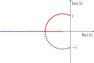
Figure 1: Representation of $\sigma(\Lambda)$. Both the plain red curve $\lambda_{+}$ and the dashed blue curve $\lambda_{-}$ touch the imaginary axis when $k=0$ in a quadratic way. When $k\to\pm\infty$, they go respectively to $\frac{-1}{\alpha}$ and $-\infty$. For small values of $k$, the two curves lie on the circle with center $-\frac{1}{\alpha}$ and radius $\sqrt{1+\frac{1}{\alpha^{2}}}$.

We note that the curves $\lambda_{\pm}\colon\mathbb{R}\to\mathbb{C}$ are confined to the left-half plane and touch the imaginary axis only at the points $\pm\mathrm{i}$ for the same frequency $k=0$. So, for small values of $k$, $\lambda_{+}(k)\neq\lambda_{-}(k)$ thus the Fourier symbol $\widehat{\Lambda}(k)$ is diagonizable. Hence, there exist $k_{0}>0$ and smooth maps $P_{\pm}\colon(-k_{0},k_{0})\to\mathbb{C}^{2\times 2}$ such that $P_{\pm}(k)$ is the spectral projection of $\widehat{\Lambda}(k)$ onto the $1$-dimensional eigenspace corresponding to the eigenvalue $\lambda_{\pm}(k)$ for $k\in(-k_{0},k_{0})$. Moreover, there exists $\theta_{1}>0$ such that it holds

(9) $$\Re(\lambda_{\pm}(k))=-\frac{1}{2}\alpha k^{2},\qquad k\in(-k_{0},k_{0}),$$

and

(10) $$\sup\Re(\sigma(\widehat{\Lambda}(k)))<-\theta_{1},\qquad k\in\mathbb{R}\setminus\left(-\frac{k_{0}}{2},\frac{k_{0}}{2}\right).$$

To separate critical from damped modes and diagonalize the system at criticality we introduce mode filters. Thus, let $\chi$ be a smooth cut-off function whose support is contained in $(-k_{0},k_{0})$ such that $\chi(k)=1$ for $k\in[-k_{0}/2,k_{0}/2]$. Given a solution $U$ of (5) we introduce the functions

(11) $$\widehat{U}_{\mathrm{c}}(t,k)=\chi(k)\widehat{U}(t,k),\qquad\qquad\widehat{U}_{\mathrm{s}}=\widehat{U}-\widehat{U}_{\mathrm{c}}.$$

In addition to separate low frequency (critical) from high frequency (damped), this decomposition also allow to separate the two critical modes. Indeed, projections $P_{\pm}$ are not well defined for $k\notin[-k_{0},k_{0}]$. Thanks to $\chi(k)=0$ for $\lvert k\rvert\geq k_{0}$, we have the decomposition

(12) $$\widehat{U}=P_{+}\widehat{U}_{\mathrm{c}}+P_{-}\widehat{U}_{\mathrm{c}}+\widehat{U}_{\mathrm{s}}.$$

3.2 Linear estimates

Our aim is to obtain estimates on the matrix exponential $\mathrm{e}^{\widehat{\Lambda}(k)t}$ for $k\in\mathbb{R}\setminus(-k_{0}/2,k_{0}/2)$ and $t\geq 0$. First, setting

$$k_{1}:=\sqrt{\frac{2+2\sqrt{1+\alpha^{2}}}{\alpha^{2}}},$$

we observe that the eigenvalues $\lambda_{+}(k)$ and $\lambda_{-}(k)$ are distinct for $k^{2}>k_{1}^{2}$ and, thus, $\widehat{\Lambda}(k)$ can be diagonalized. The associated change of basis is represented by a matrix $S(k)$, whose columns are comprised of eigenvectors of $\widehat{\Lambda}(k)$, and its inverse, which are given by

$$S(k)=\begin{pmatrix}\frac{1+k^{2}}{\mu(k)}&-\frac{1+k^{2}}{\mu(k)}\\ 1&1\end{pmatrix},\qquad S(k)^{-1}=\frac{1}{2}\begin{pmatrix}\frac{\mu(k)}{4k^{2}+4}&1\\ -\frac{\mu(k)}{4k^{2}+4}&1\end{pmatrix}.$$

One readily observes that the coefficients of $S(\cdot)$ and $S(\cdot)^{-1}$ are bounded on $\mathbb{R}\setminus(-2k_{1},2k_{1})$. On the other hand, it holds

$$\lambda_{-}(k)\leq-\dfrac{1}{2}\alpha k^{2},\qquad\lambda_{+}(k)\leq-\dfrac{1}{\alpha}$$

for $|k|>k_{1}$. We conclude that there exists $\theta_{2}>0$ such that the matrix exponential

$$\mathrm{e}^{\widehat{\Lambda}(k)t}=S(k)^{-1}\mathrm{diag}\left(\mathrm{e}^{\lambda_{+}(k)t},\mathrm{e}^{\lambda_{-}(k)t}\right)S(k),$$

obeys the estimate

(13) $$\left\|\mathrm{e}^{\widehat{\Lambda}(k)t}\right\|\lesssim\mathrm{e}^{-\theta_{2}t},\qquad k\in\mathbb{R}\setminus(-2k_{1},2k_{1}),\,t\geq 0.$$

To bound the matrix exponential $\mathrm{e}^{\widehat{\Lambda}(k)t}$ on the compact set $J:=[-2k_{1},-k_{0}/2]\cup[k_{0}/2,2k_{1}]$ we collect some facts from [1, Chapter A-III, §7]. First, since $J$ is compact and $\widehat{\Lambda}$ is continuous on $J$, the multiplication operator $A\colon f\mapsto\widehat{\Lambda}f$ generates a strongly continuous semigroup $(T(t))_{t\geq 0}$ on $C(J,\mathbb{C}^{2})$, which is given by

$$(T(t)f)(k)=\mathrm{e}^{\widehat{\Lambda}(k)t}f(k),\qquad k\in J.$$

Second, the growth bound of the semigroup $(T(t))_{t\geq 0}$ coincides with the spectral bound of $A$. Third, the spectrum of $A$ is given by

$$\sigma(A)=\bigcup_{k\in J}\sigma(\widehat{\Lambda}(k)).$$

Combining the latter three observations with (10) yields that the growth bound of the semigroup $(T(t))_{t\geq 0}$ is smaller than $-\theta_{1}$, which implies $\|\mathrm{e}^{\widehat{\Lambda(k)}t}\|\lesssim\mathrm{e}^{-\theta_{1}t}$ for all $t\geq 0$ and $k\in J$. Combining the latter with (13) yields $\theta_{0}>0$ such that

(14) $$\left\|\mathrm{e}^{\widehat{\Lambda}(k)t}\right\|\lesssim\mathrm{e}^{-\theta_{0}t},\qquad k\in\mathbb{R}\setminus\left(-\frac{k_{0}}{2},\frac{k_{0}}{2}\right),\,t\geq 0.$$

4 Space-time resonance

4.1 Resonance phases

Nonlinear terms creates interaction between linear critical modes $\left\{\chi e^{\hat{\Lambda}t}P_{+},\chi e^{\hat{\Lambda}t}P_{-}\right\}$. Whether or not the resulting interaction is further amplified by the linear dynamic will decide the long time behavior of solutions. As we shall see in the next subsection, evaluating the presence of such a resonance mechanism comes down to computation of simple objects called resonance phases.

For quadratic terms

For all $(k,l)\in\mathbb{R}^{2}$, for $j=(j_{0},j_{1},j_{2})\in\left\{-1,1\right\}^{3}$, let

$$\phi^{2}_{j}(k,l)=\lambda_{j_{0}}(k)-\lambda_{j_{1}}(k-l)-\lambda_{j_{2}}(l).$$

Heuristically, this phase vanishes when the two modes $j_{1}$ and $j_{2}$ (respectively with spatial frequency $k-l$ and $l$) interact and result in a mode $j_{0}$ with spatial frequency $k$. Due to $k=0$ being the only non-stable frequency at linear level, it will be enough to describe these phases for small values of $k$ and $l$.

Lemma 4.1.

There exists $k_{1}>0$ and $\theta_{0}>0$ such that for all $(k,l)\in[-k_{1},k_{1}]^{2}$ and all $j\in\left\{-1,1\right\}^{3}$

(15) $$\lvert\phi^{2}_{j}(k,l)\rvert\geq\theta_{0}.$$

Proof.

Remark that for all $j\in\left\{-1,1\right\}^{3}$, we have $\phi^{2}_{j}(0,0)\in\left\{-3\mathrm{i},-\mathrm{i},\mathrm{i},3\mathrm{i}\right\}$ due to $\lambda_{\pm}(0)=\pm\mathrm{i}$. Hence $\lvert\phi^{2}_{j}(0,0)\rvert\geq 1$. The lemma then follow from smoothness of $\phi^{2}_{j}$. ∎

For cubic terms

For $k\in\mathbb{R}$, for $l=(l_{1},l_{2})\in\mathbb{R}^{2}$ and $j=(j_{0},j_{1},j_{2},j_{3})\in\left\{-1,1\right\}^{4}$, let

$$\phi^{3}_{j}(k,l)=\lambda_{j_{0}}(k)-\lambda_{j_{1}}(k-l_{1})-\lambda_{j_{2}}(l_{1}-l_{2})-\lambda_{j_{3}}(l_{2}).$$

In contrast to the above computations, cubic terms do create resonances in time.

Lemma 4.2.

Denoting $\pm 1$ as simply $\pm$, let

$$\mathcal{T}={} \big{\{}(+,-,+,+),(+,+,-,+),(+,+,+,-),$$

$$\ \ (-,+,-,-),(-,-,+,-),(-,-,-,+)\big{\}}\subset\left\{-1,1\right\}^{4}.$$

Then for all $j\in\mathcal{T}$, $\phi^{3}_{j}(0,0,0)=0$. Furthermore, there exists $k_{1}>0$ and $\theta_{0}>0$ such that for all $(k,l)\in[-k_{1},k_{1}]^{3}$ and all $j\in\left\{-1,1\right\}^{4}\backslash\mathcal{T}$,

(16) $$\lvert\phi^{3}_{j}(k,l)\rvert\geq\theta_{0}.$$

Proof.

It is direct to compute that $\phi^{3}_{j}(0,0,0)\in\left\{-4\mathrm{i},-2\mathrm{i},2\mathrm{i},4\mathrm{i}\right\}$ when $j\notin\mathcal{T}$, leading to (16) at $(k,l_{1},l_{2})=(0,0,0)$. The lemma then follows from smoothness of $\phi^{3}_{j}$. ∎

4.2 Integration by parts

For quadratic terms

The exact expression of $\mathcal{N}$ in Fourier space is easily computed by insertion of (2) into (6). For $k\in\mathbb{R}$, it reads

(17) $$\mathcal{F}(\mathcal{N}(U))(k)=\int_{\mathbb{R}}N_{2}(k,l)(\widehat{U},\widehat{U})\,\mathrm{d}l+\int_{\mathbb{R}^{2}}N_{3}(k,l_{1},l_{2})(\widehat{U},\widehat{U},\widehat{U})\,\mathrm{d}l_{1}\,\mathrm{d}l_{2},$$

where $N_{2}$ and $N_{3}$ respectively account for the quadratic and cubic terms

$$N_{2}(k,l)(\widehat{U},\widehat{V}) {}\overset{\scriptscriptstyle{\mathrm{def}}}{=}\frac{\kappa}{1+k^{2}}\,\widehat{U}_{1}(k-l)\,\widehat{V}_{1}(l)\,e_{2}$$

$$N_{3}(k,l_{1},l_{2})(\widehat{U},\widehat{V},\widehat{W}) {}\overset{\scriptscriptstyle{\mathrm{def}}}{=}\frac{\beta}{1+k^{2}}\,\widehat{U}_{1}(k-l_{1})\,\widehat{V}_{1}(l_{1}-l_{2})\,\widehat{W}_{1}(l_{2})\,e_{2}.$$

For further use, we remark that

(18) $$\lvert N_{2}(k,l)(\widehat{U},\widehat{V})\rvert\lesssim\lvert\widehat{U}(k-l)\rvert\,\lvert\widehat{V}(l)\rvert.$$

$N_{2}$ being the integrand of a convolution. Similarly,

(19) $$\lvert N_{3}(k,l_{1},l_{2})(\widehat{U},\widehat{V},\widehat{W})\rvert\lesssim\lvert\widehat{U}(k-l_{1})\rvert\,\lvert\widehat{V}(l_{1}-l_{2})\rvert\,\lvert\widehat{W}(l_{2})\rvert.$$

In the duhamel formula

$$\widehat{U}(t,k)={} e^{t\hat{\Lambda}(k)}\widehat{U}_{0}(k)+\int_{0}^{t}e^{(t-\tau)\hat{\Lambda}(k)}\int_{\mathbb{R}}N_{2}(k,l)(\widehat{U}(\tau),\widehat{U}(\tau))\,\mathrm{d}l\,\mathrm{d}\tau$$

$${}+\int_{0}^{t}e^{(t-\tau)\hat{\Lambda}(k)}\int_{\mathbb{R}^{2}}N_{3}(k,l_{1},l_{2})(\widehat{U},\widehat{U},\widehat{U})\,\mathrm{d}l_{1}\,\mathrm{d}l_{2}\,\mathrm{d}\tau$$

the most dangerous term (from the point of view of long-time behavior of small solutions) is the one involving $N_{2}(k,l)(\widehat{U}_{\mathrm{c}},\widehat{U}_{\mathrm{c}})$, recall the definition of $\widehat{U}_{\mathrm{c}}$ at (11). We rely on Lemma 4.1 to replace it by a cubic contribution.

Proposition 4.3.

For $(k,l,l_{1},l_{2})\in[-k_{0},k_{0}]^{4}$ let

$$Q_{2}(k,l)(\widehat{U},\widehat{V})=\sum_{j\in\left\{-1,1\right\}^{3}} \frac{P_{j_{0}}(k)}{\phi^{2}_{j}(k,l)}N_{2}(k,l)(P_{j_{1}}\widehat{U},P_{j_{2}}\widehat{V})$$

and

$$Q_{3}(k,l_{1},l_{2})(\widehat{U},\widehat{V},\widehat{W})=\sum_{j\in\left\{-1,1\right\}^{3}} \frac{P_{j_{0}}(k)}{\phi^{2}_{j}(k,l_{2})}N_{2}(k,l_{2})\bigg{(}P_{j_{1}}N_{2}(\cdot,l_{1}-l_{2})(\widehat{U},\widehat{V}),P_{j_{2}}\widehat{W}\bigg{)}$$

$$+\frac{P_{j_{0}}(k)}{\phi^{2}_{j}(k,l_{1})}N_{2}(k,l_{1})\bigg{(}P_{j_{1}}\widehat{U},P_{j_{2}}N_{2}(\cdot,l_{2})(\widehat{V},\widehat{W})\bigg{)}.$$

Then for all $k\in[-k_{0},k_{0}]$ and $p\in[1,+\infty]$, $\widehat{U}_{\mathrm{c}}$ satisfies

$$\int_{0}^{t}e^{(t-\tau)\hat{\Lambda}(k)}\int_{\mathbb{R}} N_{2}(k,l)(\widehat{U}_{\mathrm{c}}(\tau),\widehat{U}_{\mathrm{c}}(\tau))\,\mathrm{d}l\,\mathrm{d}\tau$$

$$={} -\left[e^{(t-\tau)\hat{\Lambda}(k)}\int_{\mathbb{R}}Q_{2}(k,l)(\widehat{U}_{\mathrm{c}}(\tau),\widehat{U}_{\mathrm{c}}(\tau))\,\mathrm{d}l\right]_{0}^{t}$$

$$+\int_{0}^{t}e^{(t-\tau)\hat{\Lambda}(k)}\int_{\mathbb{R}^{2}}Q_{3}(k,l_{1},l_{2})(\widehat{U}_{\mathrm{c}}(\tau),\widehat{U}_{\mathrm{c}}(\tau),\widehat{U}_{\mathrm{c}}(\tau))\,\mathrm{d}l_{1}\,\mathrm{d}l_{2}\,\mathrm{d}\tau$$

$$+\int_{0}^{t}e^{(t-\tau)\hat{\Lambda}(k)}\mathcal{O}_{L^{p}(\mathbb{R})}\left(\lVert\widehat{U}_{\mathrm{c}}(\tau)\rVert_{L^{p}(\mathbb{R})}\lVert\widehat{U}_{\mathrm{c}}(\tau)\rVert_{L^{1}(\mathbb{R})}^{3}\right)\,\mathrm{d}\tau,$$

where the $\mathcal{O}$ term stands for a function whose $L^{p}(\mathbb{R})$ norm is bounded from above by $C\lVert\widehat{U}_{\mathrm{c}}(\tau)\rVert_{L^{p}(\mathbb{R})}\lVert\widehat{U}_{\mathrm{c}}(\tau)\rVert_{L^{1}(\mathbb{R})}^{3}$ for some constant $C>0$ independent of $U$.

Proof.

Recall that $\widehat{U}_{\mathrm{c}}$ has support in $[-k_{0},k_{0}]$, and that projections $P_{\pm}$ are well defined there (12). Thus, we can decompose the quadratic term into

$$\int_{0}^{t}e^{(t-\tau)\hat{\Lambda}(k)} \int_{\mathbb{R}}N_{2}(k,l)(\widehat{U}_{\mathrm{c}}(\tau),\widehat{U}_{\mathrm{c}}(\tau))\,\mathrm{d}l\,\mathrm{d}\tau$$

(20) $$= \sum_{j\in\left\{-1,1\right\}^{3}}\int_{0}^{t}e^{(t-\tau)\lambda_{j_{0}}(k)}\int_{\mathbb{R}}P_{j_{0}}(k)N_{2}(k,l)(P_{j_{1}}\widehat{U}_{\mathrm{c}}(\tau),P_{j_{2}}\widehat{U}_{\mathrm{c}}(\tau))\,\mathrm{d}l\,\mathrm{d}\tau.$$

Because $\lambda_{j_{0}}(k)$ never vanishes, we are able to integrate by part each summand of (20) with respect to time. Let first compute, since $N_{2}(k,l)$ is multilinear, that

$$\partial_{\tau}N_{2}(k,l)(\widehat{U},\widehat{V})=N_{2}(k,l)(\partial_{\tau}\widehat{U},\widehat{V})+N_{2}(k,l)(\widehat{U},\partial_{\tau}\widehat{V}).$$

Thus we compute, using the original equation (5) and the Fourier expression (17) of $\mathcal{N}$, that

$$\partial_{\tau}N_{2} (k,l)(P_{j_{1}}\widehat{U}_{\mathrm{c}},P_{j_{2}}\widehat{U}_{\mathrm{c}})$$

$$={} \big{(}\lambda_{j_{1}}(k-l)+\lambda_{j_{2}}(l)\big{)}N_{2}(k,l)(P_{j_{1}}\widehat{U}_{\mathrm{c}},P_{j_{2}}\widehat{U}_{\mathrm{c}})$$

(21) $${}+\int_{\mathbb{R}}N_{2}(k,l)(P_{j_{1}}N_{2}(\cdot,\tilde{l})(\widehat{U}_{\mathrm{c}},\widehat{U}_{\mathrm{c}})\,,\,P_{j_{2}}\widehat{U}_{\mathrm{c}})+N_{2}(k,l)(P_{j_{1}}\widehat{U}_{\mathrm{c}},P_{j_{2}}N_{2}(\cdot,\tilde{l})(\widehat{U}_{\mathrm{c}},\widehat{U}_{\mathrm{c}}))\,\mathrm{d}\tilde{l}$$

(22) $${}+\int_{\mathbb{R}^{2}}N_{2}(k,l)(P_{j_{1}}N_{3}(\cdot,\tilde{l}_{1},\tilde{l}_{2})(\widehat{U}_{\mathrm{c}},\widehat{U}_{\mathrm{c}},\widehat{U}_{\mathrm{c}}),P_{j_{2}}\widehat{U}_{\mathrm{c}})$$

(23) $$\hskip 30.00005pt+N_{2}(k,l)(P_{j_{1}}\widehat{U}_{\mathrm{c}},P_{j_{2}}N_{3}(\cdot,\tilde{l}_{1},\tilde{l}_{2})(\widehat{U}_{\mathrm{c}},\widehat{U}_{\mathrm{c}},\widehat{U}_{\mathrm{c}}))\,\mathrm{d}\tilde{l}_{1}\,\mathrm{d}\tilde{l}_{2}.$$

Let $j\in\left\{-1,1\right\}^{4}$. Instead of directly integrating by part the $j$-th summand of (20), we introduce a function $f_{j}:\mathbb{R}^{2}\to\mathbb{R}$ whose expression will be determined in a few lines, and integrate by part the following expression:

$$\int_{0}^{t} e^{(t-\tau)\lambda_{j_{0}}(k)}\int_{\mathbb{R}}f_{j}(k,l)\,P_{j_{0}}(k)\,N_{2}(k,l)(P_{j_{1}}\widehat{U}_{\mathrm{c}},P_{j_{2}}\widehat{U}_{\mathrm{c}})\,\mathrm{d}l\,\mathrm{d}\tau$$

$$= \left[\frac{e^{(t-\tau)\lambda_{j_{0}}(k)}}{-\lambda_{j_{0}}(k)}\int_{\mathbb{R}}f_{j}(k,l)\,P_{j_{0}}(k)\,N_{2}(k,l)(P_{j_{1}}\widehat{U}_{\mathrm{c}},P_{j_{2}}\widehat{U}_{\mathrm{c}})\,\mathrm{d}l\right]_{0}^{t}$$

(24) $${}+\int_{0}^{t}\frac{e^{(t-\tau)\lambda_{j_{0}}(k)}}{\lambda_{j_{0}}(k)}\bigg{(}\int_{\mathbb{R}}f_{j}(k,l)\,\big{(}\lambda_{j_{1}}(k-l)+\lambda_{j_{2}}(l)\big{)}\,P_{j_{0}}(k)\,N_{2}(k,l)(P_{j_{1}}\widehat{U}_{\mathrm{c}},P_{j_{2}}\widehat{U}_{\mathrm{c}})\,\mathrm{d}l$$

$${}\qquad\qquad\qquad\qquad\quad+\int_{\mathbb{R}^{2}}f_{j}(k,l)\,\tilde{Q}_{3}^{j}(k,l,\tilde{l})(\widehat{U}_{\mathrm{c}},\widehat{U}_{\mathrm{c}},\widehat{U}_{\mathrm{c}})\,\mathrm{d}l\,\mathrm{d}\tilde{l}$$

$${}\qquad\qquad\qquad\qquad\quad+\int_{\mathbb{R}^{3}}f_{j}(k,l)\big{(}Q_{4}^{j,1}(\widehat{U}_{\mathrm{c}})+Q_{4}^{j,2}(\widehat{U}_{\mathrm{c}})\big{)}\,\mathrm{d}l\,\mathrm{d}\tilde{l}_{1}\,\mathrm{d}\tilde{l}_{2}\bigg{)},$$

where $\tilde{Q}_{3}^{j}$, $Q_{4}^{j,1}$ and $Q_{4}^{j,2}$ are respectively the integrand of $P_{j_{0}}$(21), $P_{j_{0}}$(22) and $P_{j_{0}}$(23). By moving the terms (24) to the left hand side of the above equality, we can factor out a

$$1-\frac{\lambda_{j_{1}}(k-l)+\lambda_{j_{2}}(l)}{\lambda_{j_{0}}(k)}=\frac{\phi^{2}_{j}(k,l)}{\lambda_{j_{0}}(k)}.$$

Setting $f_{j}(k,l)=\frac{\lambda_{j_{0}}(k)}{\phi^{2}_{j}(k,l)}$, these terms simplify and we finally get an expression for the $j$-th summand of (20):

$$\int_{0}^{t} e^{(t-\tau)\lambda_{j_{0}}(k)}\int_{\mathbb{R}}P_{j_{0}}(k)\,N_{2}(k,l)(P_{j_{1}}\widehat{U}_{\mathrm{c}},P_{j_{2}}\widehat{U}_{\mathrm{c}})\,\mathrm{d}l\,\mathrm{d}\tau$$

$${}=-\left[e^{(t-\tau)\lambda_{j_{0}}(k)}\int_{\mathbb{R}}\frac{1}{\phi^{2}_{j}(k,l)}\,P_{j_{0}}(k)\,N_{2}(k,l)(P_{j_{1}}\widehat{U}_{\mathrm{c}},P_{j_{2}}\widehat{U}_{\mathrm{c}})\,\mathrm{d}l\right]_{0}^{t}$$

$${}\quad\,+\int_{0}^{t}e^{(t-\tau)\lambda_{j_{0}}(k)}\bigg{(}\int_{\mathbb{R}^{2}}\frac{1}{\phi^{2}_{j}(k,l)}\,\tilde{Q}_{3}^{j}(k,l,\tilde{l})(\widehat{U}_{\mathrm{c}},\widehat{U}_{\mathrm{c}},\widehat{U}_{\mathrm{c}})\,\mathrm{d}l\,\mathrm{d}\tilde{l}$$

$${}\qquad\qquad\qquad\qquad\quad+\int_{\mathbb{R}^{3}}\frac{1}{\phi^{2}_{j}(k,l)}(Q_{4}^{j,1}(\widehat{U}_{\mathrm{c}})+Q_{4}^{j,2}(\widehat{U}_{\mathrm{c}}))\,\mathrm{d}l\,\mathrm{d}\tilde{l}_{1}\,\mathrm{d}\tilde{l}_{2}\bigg{)}\mathrm{d}\tau.$$

It is direct to see from the two changes of variables $(l,\tilde{l})=(l_{2},l_{1}-l_{2})$ and $(l,\tilde{l})=(l_{1},l_{2})$ (respectively corresponding to each summand below integral (21)) that

$$\sum_{j\in\left\{-1,1\right\}^{3}}P_{j_{0}}(k)\int_{\mathbb{R}^{2}}\frac{1}{\phi^{2}_{j}(k,l)}\,\tilde{Q}_{3}^{j}(k,l,\tilde{l})(\widehat{U},\widehat{V},\widehat{W})\,\mathrm{d}l\,\mathrm{d}\tilde{l}=\int_{\mathbb{R}^{2}}Q_{3}(k,l_{1},l_{2})(\widehat{U},\widehat{V},\widehat{W})\,\mathrm{d}l_{1}\,\mathrm{d}l_{2}.$$

We now turn to the bound of higher order terms. Successively applying (18) and (19), we obtain

$$\lvert Q_{4}^{j,1}(\widehat{U}_{\mathrm{c}})\rvert\lesssim\lvert\widehat{U}_{\mathrm{c}}(k-l-\tilde{l}_{1})\rvert\,\lvert\widehat{U}_{\mathrm{c}}(\tilde{l}_{1}-\tilde{l}_{2})\rvert\,\lvert\widehat{U}_{\mathrm{c}}(\tilde{l}_{2})\rvert\,\lvert\widehat{U}_{\mathrm{c}}(l)\rvert,$$

$$\lvert Q_{4}^{j,2}(\widehat{U}_{\mathrm{c}})\rvert\lesssim\lvert\widehat{U}_{\mathrm{c}}(k-l)\rvert\,\lvert\widehat{U}_{\mathrm{c}}(l-\tilde{l}_{1})\rvert\,\lvert\widehat{U}_{\mathrm{c}}(\tilde{l}_{1}-\tilde{l}_{2})\rvert\,\lvert\widehat{U}_{\mathrm{c}}(\tilde{l}_{2})\rvert.$$

Applying the change of variables $(l_{1},l_{2},l_{3})=(l+\tilde{l}_{1},l+\tilde{l}_{2},l)$ to the first and $(l_{1},l_{2},l_{3})=(l,\tilde{l}_{1},\tilde{l}_{2})$ to the second, we get

$$\lvert Q_{4}^{j,1}(\widehat{U}_{\mathrm{c}})+Q_{4}^{j,2}(\widehat{U}_{\mathrm{c}})\rvert\lesssim\lvert\widehat{U}_{\mathrm{c}}(k-l_{1})\rvert\,\lvert\widehat{U}_{\mathrm{c}}(l_{1}-l_{2})\rvert\,\lvert\widehat{U}_{\mathrm{c}}(l_{2}-l_{3})\rvert\,\lvert\widehat{U}_{\mathrm{c}}(l_{3})\rvert.$$

Since the right hand side is the integrand of a convolution, we can use Young’s inequality:

$$\left\lVert\int_{\mathbb{R}^{3}}\frac{Q_{4}^{j,1}(\widehat{U}_{\mathrm{c}})+Q_{4}^{j,2}(\widehat{U}_{\mathrm{c}})}{\phi^{2}_{j}(\cdot,l)}\,\mathrm{d}l_{1}\,\mathrm{d}l_{2}\,\mathrm{d}l_{3}\right\rVert_{L^{p}(\mathbb{R})}\lesssim{} \left\lVert\lvert\widehat{U}_{\mathrm{c}}\rvert*\lvert\widehat{U}_{\mathrm{c}}\rvert*\lvert\widehat{U}_{\mathrm{c}}\rvert*\lvert\widehat{U}_{\mathrm{c}}\rvert\right\rVert_{L^{p}(\mathbb{R})},$$

$$\lesssim{} \lVert\widehat{U}_{\mathrm{c}}\rVert_{L^{p}(\mathbb{R})}\lVert\widehat{U}_{\mathrm{c}}\rVert_{L^{1}(\mathbb{R})}^{3}.$$

The term of order four is thus the announced $\mathcal{O}$, and the proof is complete. ∎

Relying on Lemma 4.1, it is direct to check that $Q_{3}$ satisfies a similar bound than $N_{3}$:

(25) $$\lvert Q_{3}(k,l_{1},l_{2})(\widehat{U},\widehat{V},\widehat{W})\rvert\lesssim\lvert\widehat{U}(k-l_{1})\rvert\,\lvert\widehat{V}(l_{1}-l_{2})\rvert\,\lvert\widehat{W}(l_{2})\rvert.$$

For cubic terms

After the first integration by part, the Duhamel formula for (5) reads

$$\widehat{U}(t,k)={} e^{t\hat{\Lambda}(k)}\widehat{U}_{0}(k)-\left[e^{(t-\tau)\hat{\Lambda}(k)}\int_{\mathbb{R}}Q_{2}(k,l)(\widehat{U}_{\mathrm{c}}(\tau),\widehat{U}_{\mathrm{c}}(\tau))\,\mathrm{d}l\right]_{0}^{t}$$

$$+\int_{0}^{t}e^{(t-\tau)\hat{\Lambda}(k)}\bigg{(}\int_{\mathbb{R}}N_{2}(k,l)(\widehat{U}(\tau),\widehat{U}(\tau))-N_{2}(k,l)(\widehat{U}_{\mathrm{c}}(\tau),\widehat{U}_{\mathrm{c}}(\tau))\,\mathrm{d}l$$

$$\phantom{{}+\int_{0}^{t}e^{(t-\tau)\hat{\Lambda}(k)}\bigg{(}}+\int_{\mathbb{R}^{2}}(Q_{3}+N_{3})(k,l_{1},l_{2})(\widehat{U}_{\mathrm{c}}(\tau),\widehat{U}_{\mathrm{c}}(\tau),\widehat{U}_{\mathrm{c}}(\tau))\,\mathrm{d}l_{1}\,\mathrm{d}l_{2}$$

$$\phantom{{}+\int_{0}^{t}e^{(t-\tau)\hat{\Lambda}(k)}\bigg{(}}+\mathcal{O}_{L^{p}(\mathbb{R})}\left(\lVert\widehat{U}_{\mathrm{c}}(\tau)\rVert_{L^{p}(\mathbb{R})}\lVert\widehat{U}_{\mathrm{c}}(\tau)\rVert_{L^{1}(\mathbb{R})}^{3}\right)\bigg{)}\mathrm{d}\tau.$$

As we shall see in further sections, remaining quadratic terms are not problematic, so that most dangerous term is the one involving $Q_{3}+N_{3}$. This cubic term can be further decomposed as

$$(Q_{3}+N_{3}) (k,l_{1},l_{2})(\widehat{U}(\tau),\widehat{U}(\tau),\widehat{U}(\tau))$$

$$={} \sum_{j\in\left\{-1,1\right\}^{4}}\rho_{j_{0}}(k)\,\langle\widehat{U},\rho^{*}_{j_{1}}\rangle(k-l_{1})\,\langle\widehat{U},\rho_{j_{2}}^{*}\rangle(l_{1}-l_{2})\,\langle\widehat{U},\rho^{*}_{j_{3}}\rangle(l_{2})\,\bigg{(}Q_{3}^{j}+N_{3}^{j}\bigg{)}(k,l_{1},l_{2})$$

with coefficients

$$Q_{3}^{j}(k,l_{1},l_{2})={} \langle Q_{3}(k,l_{1},l_{2})(\rho_{j_{1}},\rho_{j_{2}},\rho_{j_{3}}),\rho_{j_{0}}(k)\rangle,$$

$$N_{3}^{j}(k,l_{1},l_{2})={} \langle N_{3}(k,l_{1},l_{2})(\rho_{j_{1}},\rho_{j_{2}},\rho_{j_{3}}),\rho_{j_{0}}(k)\rangle.$$

The indices $j\in\mathcal{T}$ correspond to the time resonant terms which can not be integrated by part in time. However, it could happen that coefficients $Q_{3}^{j}(k,l_{1},l_{2})$ and $N_{3}^{j}(k,l_{1},l_{2})$ cancel each other. If all resonant terms cancels out, the remaining terms can be integrated by part once more, and global existence of solution is easily obtain by a standard modification of the nonlinear iteration scheme below. In the following Lemma, we check that such cancellation can not happen simultaneously for all resonant indices, in the setting of the viscous Klein-Gordon equation.

Let us comment that cancellation for all $(k,l_{1},l_{2})\in\left\{0\right\}\times\mathbb{R}^{2}$ would be enough to close the non-linear iteration. In the present situation, inspection of coefficients at $(k,l_{1},l_{2})=(0,0,0)$ is enough to obtain a negative result.

Lemma 4.4.

With the above notations, for all $j\in\left\{-1,1\right\}^{4}$,

$$N_{3}^{j}(0,0,0)={} \beta\,\frac{j_{0}}{2\mathrm{i}},$$

$$Q_{3}^{j}(0,0,0)={} \kappa^{2}\,\frac{j_{0}}{2\mathrm{i}}\sum_{h\in\left\{-1,1\right\}}\frac{h}{2\mathrm{i}}\left(\frac{1}{\phi^{2}_{j_{0}hj_{3}}(0,0)}+\frac{1}{\phi^{2}_{j_{0}j_{1}h}(0,0)}\right).$$

These expressions reduce to the following table of numerical values.

$$\begin{array}[]{|c|c|c|}\hline\cr j&N_{3}^{j}(0,0,0)&Q_{3}^{j}(0,0,0)\\[1.99997pt] \hline\cr(+,-,+,+)&\frac{\beta}{2\mathrm{i}}&\frac{\kappa^{2}}{2\mathrm{i}}\cdot\frac{2}{3}\\[1.99997pt] \hline\cr(+,+,-,+)&\frac{\beta}{2\mathrm{i}}&\frac{\kappa^{2}}{2\mathrm{i}}\cdot 2\\[1.99997pt] \hline\cr(+,+,+,-)&\frac{\beta}{2\mathrm{i}}&\frac{\kappa^{2}}{2\mathrm{i}}\cdot\frac{2}{3}\\[1.99997pt] \hline\cr\end{array}$$

The coefficients that correspond to remaining indices $j\in\mathcal{T}$ are easily obtained from the relations $N_{3}^{-j}(0,0,0)=-N_{3}^{j}(0,0,0)$ and $Q_{3}^{-j}(0,0,0)=-Q_{3}^{j}(0,0,0)$. In particular, the system of equation

$$N_{3}^{j}(0,0,0)+Q_{3}^{j}(0,0,0)=0,\hskip 40.00006pt\forall j\in\mathcal{T}$$

admits no other solution than $(\kappa,\beta)=(0,0)$.

Proof.

It is quite direct to compute that

$$N_{3}(0,0,0)(\rho_{j_{1}},\rho_{j_{2}},\rho_{j_{3}})=\beta e_{2}.$$

Decomposing $e_{2}$ as $e_{2}=\frac{1}{2\mathrm{i}}\left(\rho_{+}(0)-\rho_{-}(0)\right)$ gives the claimed expresion of $N_{3}^{j}(0,0,0)$. We now turn to the computation of $Q_{3}^{j}(0,0,0)$. From definition of $Q_{3}$, we see that

$$P_{j_{0}}(0)Q_{3}(0,0,0) (\rho_{j_{1}},\rho_{j_{2}},\rho_{j_{3}})$$

$$={} P_{j_{0}}(0)\sum_{h\in\left\{-1,1\right\}^{3}}\frac{P_{h_{0}}(0)}{\phi^{2}_{h}(0,0)}N_{2}(0,0)\bigg{(}P_{h_{1}}N_{2}(\cdot,0)(\rho_{j_{1}},\rho_{j_{2}}),P_{h_{2}}\rho_{j_{3}}\bigg{)}$$

$$\hskip 70.0001pt{}+\frac{P_{h_{0}}(0)}{\phi^{2}_{h}(0,0)}N_{2}(0,0)\bigg{(}P_{h_{1}}\rho_{j_{1}},P_{h_{2}}N_{2}(\cdot,0)(\rho_{j_{2}},\rho_{j_{3}})\bigg{)},$$

$$={} \sum_{h_{1}\in\left\{-1,1\right\}}\frac{P_{j_{0}}(0)}{\phi^{2}_{j_{0}h_{1}j_{3}}(0,0)}N_{2}(0,0)\bigg{(}P_{h_{1}}N_{2}(\cdot,0)(\rho_{j_{1}},\rho_{j_{2}}),\rho_{j_{3}}\bigg{)}$$

$${}+\sum_{h_{2}\in\left\{-1,1\right\}}\frac{P_{j_{0}}(0)}{\phi^{2}_{j_{0}j_{1}h_{2}}(0,0)}N_{2}(0,0)\bigg{(}\rho_{j_{1}},P_{h_{2}}N_{2}(\cdot,0)(\rho_{j_{2}},\rho_{j_{3}})\bigg{)}.$$

At this point, let us recall that $N_{2}(0,0)(\rho_{j_{1}},\rho_{j_{2}})=\kappa\,e_{2}$, and that $P_{h_{1}}(0)e_{2}=\frac{h_{1}}{2\mathrm{i}}\rho_{h_{1}}(0)$. This allow to considerably reduce the above:

$$P_{j_{0}}(0)Q_{3}(0,0,0) (\rho_{j_{1}},\rho_{j_{2}},\rho_{j_{3}})$$

$$={} \sum_{h_{1}\in\left\{-1,1\right\}}\kappa^{2}\frac{P_{j_{0}}(0)}{\phi^{2}_{j_{0}h_{1}j_{3}}(0,0)}\frac{h_{1}}{2\mathrm{i}}e_{2}\ +\sum_{h_{2}\in\left\{-1,1\right\}}\kappa^{2}\frac{P_{j_{0}}(0)}{\phi^{2}_{j_{0}j_{1}h_{2}}(0,0)}\frac{h_{2}}{2\mathrm{i}}e_{2},$$

$$={} \frac{j_{0}}{2\mathrm{i}}\,\rho_{j_{0}}(0)\,\kappa^{2}\sum_{h\in\left\{-1,1\right\}}\frac{h}{2\mathrm{i}}\left(\frac{1}{\phi^{2}_{j_{0}hj_{3}}(0,0)}+\frac{1}{\phi^{2}_{j_{0}j_{1}h}(0,0)}\right),$$

which is the claimed expression of $Q_{3}^{j}$. The table is easily obtained by explicit computations, for example:

$$\frac{2\mathrm{i}}{\kappa^{2}}M_{+-++}=\frac{1}{2\mathrm{i}}\left(\frac{1}{\phi^{2}_{+++}}+\frac{1}{\phi^{2}_{+-+}}-\frac{1}{\phi^{2}_{+-+}}-\frac{1}{\phi^{2}_{+--}}\right)=\frac{1}{2\mathrm{i}}\left(\frac{1}{-\mathrm{i}}-\frac{1}{3\mathrm{i}}\right)=\frac{2}{3}.$$

The relation on $Q_{3}^{-j}(0,0,0)$ comes from the change of variable $h\to-h$ and the fact that $\phi^{2}_{-j}(0,0)=-\phi^{2}_{j}(0,0)$. ∎

Remark 4.5.

In the above Lemma, the fact that $N_{3}^{j}(0,0,0)$ and $Q_{3}^{j}(0,0,0)$ can not coincide should be no surprise. Indeed, while $N_{3}(\widehat{U},\widehat{V},\widehat{W})$ contains an internal symmetry with respect to $\widehat{U}$, $\widehat{V}$ and $\widehat{W}$, the term $Q_{3}(\widehat{U},\widehat{V},\widehat{W})$ lacks a $N_{2}(\widehat{V},N_{2}(\widehat{U},\widehat{W}))$ summand to exhibit the same symmetry.

5 Nonlinear integral scheme

To lighten notations, we use nonlinear notations rather than multilinear ones. Let

$$\mathcal{N}_{2}(\widehat{U})(k)={} \int_{\mathbb{R}}N_{2}(k,l)(\widehat{U},\widehat{U})\,\mathrm{d}l,$$

$$\mathcal{N}_{3}(\widehat{U})(k)={} \int_{\mathbb{R}_{2}}N_{3}(k,l_{1},l_{2})(\widehat{U},\widehat{U},\widehat{U})\,\mathrm{d}l_{1}\,\mathrm{d}l_{2},$$

$$\mathcal{Q}_{2}(\widehat{U})(k)={} \int_{\mathbb{R}}Q_{2}(k,l)(\widehat{U},\widehat{U})\,\mathrm{d}l,$$

$$\mathcal{Q}_{3}(\widehat{U})(k)={} \int_{\mathbb{R}_{2}}Q_{3}(k,l_{1},l_{2})(\widehat{U},\widehat{U},\widehat{U})\,\mathrm{d}l_{1}\,\mathrm{d}l_{2}.$$

Then from the previous section, the Duhamel formula for solutions of (5) reads

$$\widehat{U}(t,k)={} e^{t\hat{\Lambda}(k)}\widehat{U}_{0}(k)-\left[e^{(t-\tau)\hat{\Lambda}(k)}\mathcal{Q}_{2}(\widehat{U}_{\mathrm{c}}(\tau))(k)\right]_{0}^{t}$$

(26) $${}+\int_{0}^{t}e^{(t-\tau)\hat{\Lambda}(k)}\bigg{(}\mathcal{N}_{2}(\widehat{U}(\tau))(k)-\mathcal{N}_{2}(\widehat{U}_{\mathrm{c}}(\tau))(k)+\mathcal{N}_{3}(\widehat{U}(\tau))(k)$$

$$\phantom{{}+\int_{0}^{t}e^{(t-\tau)\hat{\Lambda}(k)}\bigg{(}}+\mathcal{Q}_{3}(\widehat{U}_{\mathrm{c}}(\tau))(k)+\mathcal{O}_{L^{p}}\left(\lVert\widehat{U}_{\mathrm{c}}(\tau)\rVert_{L^{p}}\lVert\widehat{U}_{\mathrm{c}}(\tau)\rVert_{L^{1}}^{3}\right)\bigg{)}\mathrm{d}\tau.$$

5.1 Nonlinear bounds

Young’s inequality allow to convert the pointwise bounds (19) and (25) into the following convolution bounds:

(27) $$\lVert\mathcal{N}_{3}(\widehat{U})\rVert_{L^{p}(\mathbb{R})}+\lVert\mathcal{Q}_{3}(\widehat{U}_{\mathrm{c}})\rVert_{L^{p}(\mathbb{R})}\lesssim\lVert\widehat{U}\rVert_{L^{p}(\mathbb{R})}\lVert\widehat{U}\rVert_{L^{1}(\mathbb{R})}^{2}.$$

Similarly, using the pointwise bound (18) together with the non-resonance property (15), we obtain

(28) $$\lVert\mathcal{N}_{2}(\widehat{U})\rVert_{L^{p}(\mathbb{R})}+\lVert\mathcal{Q}_{2}(\widehat{U}_{\mathrm{c}})\rVert_{L^{p}(\mathbb{R})}\lesssim\lVert\widehat{U}\rVert_{L^{p}(\mathbb{R})}\lVert\widehat{U}\rVert_{L^{1}(\mathbb{R})}.$$

Using that $N_{2}(k,l)$ is multilinear, we also obtain

(29) $$\lVert\mathcal{N}_{2}(\widehat{U}_{\mathrm{c}}+\widehat{U}_{\mathrm{s}})-\mathcal{N}_{2}(\widehat{U}_{\mathrm{c}})\rVert_{L^{p}(\mathbb{R})}\lesssim\lVert\widehat{U}_{\mathrm{c}}\rVert_{L^{p}(\mathbb{R})}\lVert\widehat{U}_{\mathrm{s}}\rVert_{L^{1}(\mathbb{R})}+\lVert\widehat{U}_{\mathrm{s}}\rVert_{L^{p}(\mathbb{R})}\lVert\widehat{U}_{\mathrm{s}}\rVert_{L^{1}(\mathbb{R})}.$$

5.2 Proof of the main result

Proof of Theorem 1.1.

First, note that the pseudoderivatives $\partial_{x}^{j}\left(1-\partial_{x}^{2}\right)^{-1}$ for $j=0,2$ are bounded linear operators on $X_{0}$ of norm $\leq 1$. Hence,

$$v_{0}=\left(1-\partial_{x}^{2}\right)^{-1}w_{0}-\frac{\alpha}{2}\partial_{x}^{2}\left(1-\partial_{x}^{2}\right)^{-1}u_{0}$$

is a well-defined element of $X_{0}$ satisfying

$$\|v_{0}\|_{X_{0}}\leq\|w_{0}\|_{X_{0}}+\frac{\alpha}{2}\|u_{0}\|_{X_{0}}\leq\left(1+\frac{\alpha}{2}\right)\varepsilon.$$

Set $U_{0}:=(u_{0},v_{0})^{\top}$. By the local well-posedness result in §2 there exist $T_{\max}\in(0,\infty]$ and a unique, maximally defined classical solution

$$U\in C\big{(}[0,T_{\max}),X_{0}\big{)}\cap C^{2}\big{(}(0,T_{\max}),X_{0}\big{)}\cap C\big{(}(0,T_{\max}),X_{4}\big{)},$$

of (5) with initial condition $U(0)=U_{0}$. If $T_{\max}<\infty$, then it holds

$$\lim_{t\uparrow T_{\max}}\|U(t)\|_{X_{0}}=\infty.$$

Hence, we find that the template function $\eta\colon[0,T_{\max})\to\mathbb{R}$ given by

$$\eta(t)=\sup_{\tau\in[0,t]} \lVert\widehat{U}_{\mathrm{c}}(\tau)\rVert_{L^{\infty}(\mathbb{R})}+(1+\tau)^{1/2}\lVert\widehat{U}_{\mathrm{c}}(\tau)\rVert_{L^{1}(\mathbb{R})}$$

$${}+(1+\tau)^{1/2}\lVert\widehat{U}_{\mathrm{s}}(\tau)\rVert_{L^{\infty}(\mathbb{R})}+(1+\tau)\lVert\widehat{U}_{\mathrm{s}}(\tau)\rVert_{L^{1}(\mathbb{R})}$$

is well-defined, continuous, monotonically increasing and, if $T_{\max}<\infty$, then it satisfies

(30) $$\lim_{t\uparrow T_{\max}}\eta(t)=\infty.$$

Set $E_{0}:=\lVert U_{0}\rVert_{X_{0}}\leq\varepsilon$ and let $t\in[0,T_{\max})$ be such that $\eta(t)\leq 1$. We estimate the right-hand side of the Duhamel formula (26). From the bounds (9) and (10) on the spectrum of $\hat{\Lambda}(k)$, we obtain

$$\lVert\widehat{U}_{\mathrm{c}}(t)\rVert_{L^{1}(\mathbb{R})}\lesssim{} \frac{\lVert\widehat{U}_{0}\rVert_{L^{\infty}\cap L^{1}(\mathbb{R})}+\lVert\mathcal{Q}_{2}(\widehat{U}_{\mathrm{c}}(0))\rVert_{L^{\infty}\cap L^{1}(\mathbb{R})}}{(1+t)^{1/2}}+\lVert\mathcal{Q}_{2}(\widehat{U}_{\mathrm{c}}(t))\rVert_{L^{1}(\mathbb{R})}$$

$${}+\int_{0}^{t}\frac{1}{\sqrt{t-\tau}}\bigg{(}\lVert\mathcal{N}_{2}(\widehat{U}(\tau))-\mathcal{N}_{2}(\widehat{U}_{\mathrm{c}}(\tau))\rVert_{L^{\infty}(\mathbb{R})}+\lVert\mathcal{N}_{3}(\widehat{U}(\tau))\rVert_{L^{\infty}(\mathbb{R})}$$

$${}\qquad\qquad\qquad\quad+\lVert\mathcal{Q}_{3}(\widehat{U}_{\mathrm{c}}(\tau))\rVert_{L^{\infty}(\mathbb{R})}+\lVert\widehat{U}_{\mathrm{c}}(\tau)\rVert_{L^{\infty}(\mathbb{R})}\lVert\widehat{U}_{\mathrm{c}}(\tau)\rVert_{L^{1}(\mathbb{R})}^{3}\bigg{)}\mathrm{d}\tau.$$

Then applying the nonlinear estimates (27) to (29) it becomes

$$\lVert\widehat{U}_{\mathrm{c}}(t)\rVert_{L^{1}(\mathbb{R})}\lesssim{} \frac{\lVert\widehat{U}_{0}\rVert_{L^{\infty}\cap L^{1}(\mathbb{R})}+\lVert\widehat{U}_{0}\rVert_{L^{\infty}\cap L^{1}(\mathbb{R})}\lVert\widehat{U}_{0}\rVert_{L^{1}(\mathbb{R})}}{(1+t)^{1/2}}+\lVert\widehat{U}_{\mathrm{c}}(t)\rVert_{L^{1}(\mathbb{R})}^{2}$$

$${}+\int_{0}^{t}\frac{1}{\sqrt{t-\tau}}\left(\lVert\widehat{U}(\tau)\rVert_{L^{\infty}(\mathbb{R})}\lVert\widehat{U}_{\mathrm{s}}(\tau)\rVert_{L^{1}(\mathbb{R})}+\lVert\widehat{U}(\tau)\rVert_{L^{\infty}(\mathbb{R})}\lVert\widehat{U}(\tau)\rVert_{L^{1}(\mathbb{R})}^{2}\right)\mathrm{d}\tau$$

$$\lesssim{} \frac{E_{0}}{(1+t)^{1/2}}+\frac{\eta(t)^{2}}{1+t}+\int_{0}^{t}\frac{\eta(\tau)^{2}}{\sqrt{t-\tau}(1+\tau)}\mathrm{d}\tau$$

$$\lesssim{} \frac{E_{0}+\eta(t)^{2}\ln(2+t)}{(1+t)^{1/2}}.$$

In a very similar way, we bound the three other terms of the expression of $\eta$. Remark that the $\mathcal{O}$ term can always be absorbed into $\mathcal{Q}_{3}$ and $\mathcal{N}_{3}$. We obtain successively

$$\lVert\widehat{U}_{\mathrm{c}}(t)\rVert_{L^{\infty}(\mathbb{R})}\lesssim{} \lVert\widehat{U}_{0}\rVert_{L^{\infty}}+\lVert\widehat{U}_{0}\rVert_{L^{\infty}(\mathbb{R})}\lVert\widehat{U}_{0}\rVert_{L^{1}(\mathbb{R})}+\frac{\eta(t)^{2}}{(1+t)^{1/2}}+\int_{0}^{t}\frac{\eta(\tau)^{2}}{1+\tau}\mathrm{d}\tau$$

$$\lesssim{} E_{0}+\eta(t)^{2}\ln(2+t),$$

$$\lVert\widehat{U}_{\mathrm{s}}(t)\rVert_{L^{\infty}(\mathbb{R})}\lesssim{} e^{-\theta_{0}t}\lVert\widehat{U}_{0}\rVert_{L^{\infty}(\mathbb{R})}(1+\lVert\widehat{U}_{0}\rVert_{L^{1}(\mathbb{R})})+\frac{\eta(t)^{2}}{(1+t)^{1/2}}+\int_{0}^{t}\frac{e^{-\theta_{0}(t-\tau)}\eta(\tau)^{2}}{1+\tau}\mathrm{d}\tau$$

$$\lesssim{} \frac{E_{0}+\eta(t)^{2}}{(1+t)^{1/2}}.$$

Finally, we bound

$$\lVert\widehat{U}_{\mathrm{s}}(t)\rVert_{L^{1}(\mathbb{R})}\lesssim{} e^{-\theta_{0}t}\left(\lVert\widehat{U}_{0}\rVert_{L^{1}(\mathbb{R})}+\lVert\mathcal{Q}_{2}(\widehat{U}_{\mathrm{c}}(0))\rVert_{L^{1}(\mathbb{R})}\right)+\lVert\mathcal{Q}_{2}(\widehat{U}_{\mathrm{c}}(t))\rVert_{L^{1}(\mathbb{R})}$$

$${}+\int_{0}^{t}e^{-\theta_{0}(t-\tau)}\bigg{(}\lVert\mathcal{N}_{2}(\widehat{U}(\tau))-\mathcal{N}_{2}(\widehat{U}_{\mathrm{c}}(\tau))\rVert_{L^{1}(\mathbb{R})}+\lVert\mathcal{N}_{3}(\widehat{U}(\tau))\rVert_{L^{1}(\mathbb{R})}$$

$$\phantom{{}+\int_{0}^{t}e^{-\theta_{0}(t-\tau)}\bigg{(}}+\lVert\mathcal{Q}_{3}(\widehat{U}_{\mathrm{c}}(\tau))\rVert_{L^{1}(\mathbb{R})}+\lVert\widehat{U}_{\mathrm{c}}(\tau)\rVert_{L^{1}}^{4}\bigg{)}\mathrm{d}\tau$$

$$\lesssim{} e^{-\theta_{0}t}\lVert\widehat{U}_{0}\rVert_{L^{1}(\mathbb{R})}(1+\lVert\widehat{U}_{0}\rVert_{L^{1}(\mathbb{R})})+\frac{\eta(t)^{2}}{1+t}+\int_{0}^{t}\frac{e^{-\theta_{0}(t-\tau)}\eta(\tau)^{2}}{(1+\tau)^{3/2}}\mathrm{d}\tau$$

$$\lesssim{} \frac{E_{0}+\eta(t)^{2}}{1+t}.$$

Combining the latter four estimates yields a constant $C\geq 1$ such that for all $t\in[0,T_{\max})$ with $\eta(t)\leq 1$ it holds

(31) $$\eta(t)\leq C\left(E_{0}+\eta(t)^{2}\ln(2+t)\right).$$

Thus, taking

$$\varepsilon_{0}<\frac{1}{4C^{2}},\qquad M_{0}=2C,$$

it follows by the continuity, monotonicity and non-negativity of $\eta$ that, provided $\varepsilon\in(0,\varepsilon_{0})$, we have $\eta(t)\leq M_{0}\varepsilon=2C\varepsilon\leq 1$ for all $t\in[0,T_{\max})\cap\big{[}0,T_{\varepsilon}\big{]}$ with $T_{\varepsilon}=\mathrm{e}^{\varepsilon_{0}/\varepsilon}-2$. Indeed, given $t\in[0,T_{\max})\cap\big{[}0,T_{\varepsilon}\big{]}$ with $\eta(\tau)\leq 2C\varepsilon$ for each $\tau\in[0,t]$, we arrive at

$$\eta(t)\leq C\left(\varepsilon+4C^{2}\varepsilon^{2}\ln(2+t)\right)<2C\varepsilon,$$

by estimate (31) and the fact that $4C^{2}\varepsilon\ln(2+t)<1$. Thus, if (31) is satisfied, then we have $\eta(t)\leq 2C\varepsilon$, for all $t\in[0,T_{\max})\cap\big{[}0,T_{\varepsilon}\big{]}$, which implies by (30) that it must hold $T_{\max}>T_{\varepsilon}$. Consequently, $\eta(t)\leq M_{0}\varepsilon$ is satisfied for all $t\in\big{[}0,T_{\varepsilon}\big{]}$. Finally,

$$\left\|u(t)\right\|_{L^{\infty}}\leq\|U(t)\|_{L^{\infty}}\leq\lVert\widehat{U}(t)\rVert_{L^{1}}\leq\frac{M_{0}\varepsilon}{\sqrt{1+t}}$$

completes the proof by noticing that the first coordinate $u(t)=U_{1}(t)$ of $U(t)$ solves (3) by construction and $\partial_{t}u(t)=\left(1-\partial_{x}^{2}\right)U_{2}(t)+\frac{\alpha}{2}\partial_{x}^{2}U_{1}(t)\in C\big{(}[0,T_{\varepsilon}],X_{2}\big{)}$. ∎

Remark 5.1.

We observe that for the nonlinear equation, high frequencies decay is dictated by the one of low frequencies, in contrast with the linear setting. This connection arises from the integration by part in time, and more precisely from the boundary term $\mathcal{Q}_{2}(\widehat{U}_{\mathrm{c}}(t))$, that never benefits from the semigroup decay.

Remark 5.2.

We comment that to obtain the bound on $\lVert\widehat{U}_{\mathrm{s}}(t)\rVert_{L^{1}(\mathbb{R})}$, the $\mathcal{O}$ term have to be estimated in $L^{1}(\mathbb{R})$. Indeed, the Fourier multiplier associated with the semigroup does not belong to $L^{1}(\mathbb{R})$ since the eigenvalue $\lambda_{+}(k)$ is bounded when $k\to\pm\infty$. This fact alone prevents the use of a generic nonlinear term $N(u)=\kappa u^{2}+\beta u^{3}+\mathcal{O}(u^{4})$. Indeed, a $\mathcal{O}(u^{4})$ term would typically lack a convolution structure in Fourier side, and thus could not be bounded in $L^{1}(\mathbb{R})$.

6 Discussion on multiple integration by parts

In the above, we saw that cubic terms are time resonant due to vanishing of $\phi^{3}_{j}(0,0,0)$ for $j\in\mathcal{T}$. We remark that integration by part in time is still allowed since $\lambda_{\pm}$ never vanishes. Doing so typically creates a singularity, e.g.

$$\lvert\phi^{3}_{+-++}(k,l_{1},l_{2})\rvert^{-1}\geq(k^{2}+l_{1}^{2}+l_{2}^{2})^{-1}.$$

Indeed, the quadratic touching between $\lambda_{\pm}(k)$ and the imaginary axis guaranty that $\phi^{3}_{+-++}$ vanishes at least at order two. Together with this singularity, integration by parts improve terms by providing an extra integral and an extra power of $\widehat{U}$.

One could be tempted to use the integral to compensate for the singularity, and save the extra power of $\widehat{U}$ to close the non-linear scheme. In this direction, it is even possible to do a third integration by parts (quartic terms, as any even power, or non-resonant), thus improving our current scheme by two integrals, two powers of $\widehat{U}$, and a singularity of order at least $2$ spreaded along lines, e.g. $(k^{2}+l_{1}^{2}+l_{3}^{2})^{-1}$ along $\left\{k=l_{1}=l_{3}=0\right\}\subset\mathbb{R}^{4}$.

However, our conclusions in this direction are fruitless, for the following reasons. Although we do gain powers of $\widehat{U}$, recall that we work in frequency space, so that the usual role of $L^{\infty}(\mathbb{R})$ and $L^{1}(\mathbb{R})$ are exchanged when it comes down to temporal decay of linear dynamic. In particular, the decay is not provided by powers of $\widehat{U}$, but rather by integrals, and more precisely by the convolution structure. Thus, using two integral to erase the singularity precisely unwrap the improved decay that is expected between a cubic and quintic nonlinearity.

Finally, let us mention that global existence would be available in cases where the loss in singularity is strictly less than the gain in integrability, e.g. when space-resonance is available, or in presence of a transparency condition. As commented above, the former is excluded here, while Lemma 4.4 ensures that no transparency condition arises.

References

- [1] W. Arendt, A. Grabosch, G. Greiner, U. Groh, H. P. Lotz, U. Moustakas, R. Nagel, F. Neubrander, and U. Schlotterbeck. One-parameter semigroups of positive operators, volume 1184 of Lecture Notes in Mathematics. Springer-Verlag, Berlin, 1986.
- [2] P. Aviles and J. Sandefur. Nonlinear second order equations with applications to partial differential equations. J. Differential Equations, 58(3):404–427, 1985.
- [3] J. D. Avrin. Convergence properties of the strongly damped nonlinear Klein-Gordon equation. J. Differential Equations, 67(2):243–255, 1987.
- [4] B. de Rijk and G. Schneider. Global existence and decay in multi-component reaction-diffusion-advection systems with different velocities: oscillations in time and frequency. NoDEA Nonlinear Differential Equations Appl., 28(1):Paper No. 2, 38, 2021.
- [5] M. D’Abbicco and R. Ikehata. Asymptotic profile of solutions for strongly damped Klein-Gordon equations. Math. Methods Appl. Sci., 42(7):2287–2301, 2019.
- [6] M. D’Abbicco, R. Ikehata, and H. Takeda. Critical exponent for semi-linear wave equations with double damping terms in exterior domains. NoDEA Nonlinear Differential Equations Appl., 26(6):Paper No. 56, 25, 2019.
- [7] J.-M. Delort. Minoration du temps d’existence pour l’équation de Klein-Gordon non-linéaire en dimension 1 d’espace. Ann. Inst. H. Poincaré C Anal. Non Linéaire, 16(5):563–591, 1999.
- [8] L. Garénaux and B. de Rijk. Global existence and decay of small solutions in a viscous half klein–gordon equation. CRC 1173 Preprint 2022/80, Karlsruhe Institute of Technology, preprint.
- [9] W. Gordon. Der Comptoneffekt nach der Schrödingerschen Theorie. Z. Phys., 40:117–133, 1926.
- [10] N. Hayashi and P. I. Naumkin. The initial value problem for the quadratic nonlinear Klein-Gordon equation. Adv. Math. Phys., pages Art. ID 504324, 35, 2010.
- [11] N. Hayashi and P. I. Naumkin. Quadratic nonlinear Klein-Gordon equation in one dimension. J. Math. Phys., 53(10):103711, 36, 2012.
- [12] S. Katayama. A note on global existence of solutions to nonlinear Klein-Gordon equations in one space dimension. J. Math. Kyoto Univ., 39(2):203–213, 1999.
- [13] M. Keel and T. Tao. Small data blow-up for semilinear Klein-Gordon equations. Amer. J. Math., 121(3):629–669, 1999.
- [14] O. Klein. Quantentheorie und fünfdimensionale relativitätstheorie. Zeitschrift für Physik, 37(12):895–906, Dec 1926.
- [15] T.-P. Liu and Y. Zeng. Large time behavior of solutions for general quasilinear hyperbolic-parabolic systems of conservation laws. Mem. Amer. Math. Soc., 125(599):viii+120, 1997.
- [16] A. Lunardi. Analytic semigroups and optimal regularity in parabolic problems. Progress in Nonlinear Differential Equations and their Applications, 16. Birkhäuser Verlag, Basel, 1995.
- [17] K. Moriyama. Normal forms and global existence of solutions to a class of cubic nonlinear Klein-Gordon equations in one space dimension. Differential Integral Equations, 10(3):499–520, 1997.
- [18] K. Moriyama, S. Tonegawa, and Y. Tsutsumi. Almost global existence of solutions for the quadratic semilinear Klein-Gordon equation in one space dimension. Funkc. Ekvacioj, Ser. Int., 40(2):313–333, 1997.
- [19] Y. Shibata. On the rate of decay of solutions to linear viscoelastic equation. Math. Methods Appl. Sci., 23(3):203–226, 2000.
- [20] H. Sunagawa. On global small amplitude solutions to systems of cubic nonlinear Klein-Gordon equations with different mass terms in one space dimension. J. Differential Equations, 192(2):308–325, 2003.