An Extended ADMM for Three-block Nonconvex Nonseparable Problem with Applications

Abstract

We consider a three-block alternating direction method of multipliers (ADMM) for solving the nonconvex nonseparable optimization problem with linear constraint. Inspired by [1], the third variable is updated twice in each iteration to ensure the global convergence. Based on the powerful Kurdyka-Łojasiewicz property, we prove that the sequence generated by the ADMM converges globally to the critical point of the augmented Lagrangian function. We also point out the convergence of proposed ADMM with swapping the update order of the first and second variables, and with adding a proximal term to the first variable for more general nonseparable problems, respectively. Moreover, we make numerical experiments on three nonconvex problems: multiple measurement vector (MMV), robust PCA (RPCA) and nonnegative matrix completion (NMC). The results show the efficiency and outperformance of proposed ADMM.
keywords ADMM, nonconvex nonseparable optimization, global convergence, Kurdyka-Łojasiewicz property

1 Introduction

In this paper, we consider the following nonconvex nonseparable optimization problem:

$$\min_{X,Y,Z} \Phi(X)+\Psi(Y)+f(Z)+H(X,Y,Z)$$ (1.1)

$$\mathrm{s.t.} \mathcal{A}(X)+\mathcal{B}(Y)+\mathcal{C}(Z)=D,$$

where $\Phi:\mathbb{R}^{m\times n}\to\mathbb{R}\cup\{+\infty\}$ is proper lower semicontinuous, and possibly nonsmooth, nonconvex. $\Psi:\mathbb{R}^{m\times n}\to\mathbb{R}\cup\{+\infty\}$ is convex, and possibly nonsmooth. $f:\mathbb{R}^{m\times n}\to\mathbb{R}$ is Lipschitz continuously differentiable with the modulus $L_{f}>0$, and possibly nonconvex. $H:\mathbb{R}^{m\times n}\times\mathbb{R}^{m\times n}\times\mathbb{R}^{m\times n}\to\mathbb{R}$ is smooth. $\mathcal{A},\mathcal{B},\mathcal{C}:\mathbb{R}^{m\times n}\to\mathbb{R}^{d_{1}\times d_{2}}$ are linear operators, and $D\in\mathbb{R}^{d_{1}\times d_{2}}$ is a given matrix. Note that $X$, $Y$, and $Z$ can have different dimensions, as long as the operators $\mathcal{A}$, $\mathcal{B}$, and $\mathcal{C}$ map each of them to the same dimension. Here we let $X$, $Y$, and $Z$ have the same dimension only for ease of exposition. Various practical problems can be reduced to the special case of (1.1), such as compressed sensing [2, 3, 4], low-rank matrix sensing [5, 6, 7], robust principle component analysis [8, 9, 10] and so on. The augmented Lagrangian function of problem (1.1) is defined as:

$$\mathcal{L}_{\beta}(X,Y,Z,\Lambda):= \Phi(X)+\Psi(Y)+f(Z)+H(X,Y,Z)$$ (1.2)

$$-\langle\Lambda,\mathcal{A}(X)+\mathcal{B}(Y)+\mathcal{C}(Z)-D\rangle+\frac{\beta}{2}\|\mathcal{A}(X)+\mathcal{B}(Y)+\mathcal{C}(Z)-D\|_{F}^{2},$$

where $\Lambda\in\mathbb{R}^{m\times n}$ is the Lagrangian multiplier, and $\beta>0$ is the penalty parameter.

As an efficient algorithm for solving separable problems deriving from the Douglas–Rachford splitting method [11, 12], the classic ADMM [13, 14] for solving problem (1.1) uses the following Gauss-Seidel format iterations,

$$(1.3)\quad X^{k+1}\in\arg\min_{X}\mathcal{L}_{\beta}(X,Y^{k},Z^{k},\Lambda^{k}),$$

$$(1.3)\quad Y^{k+1}\in\arg\min_{Y}\mathcal{L}_{\beta}(X^{k+1},Y,Z^{k},\Lambda^{k}),$$

$$(1.3)\quad Z^{k+1}=\arg\min_{Z}\mathcal{L}_{\beta}(X^{k+1},Y^{k+1},Z,\Lambda^{k}),$$

$$(1.3)\quad \Lambda^{k+1}=\Lambda^{k}-\beta(\mathcal{A}(X^{k+1})+\mathcal{B}(Y^{k+1})+\mathcal{C}(Z^{k+1})-D).$$

When the Lipschitz part $f\equiv 0$, the nonseparable part $H\equiv 0$ and $\Phi$, $\Psi$ are proper closed convex functions, (1) reduces to the classic two-block ADMM which is designed for two-block separable convex optimization problems. For ADMM being applied on this class of problems, there has been a large body of literature studying its convergence and convergence rate [15, 16, 17, 18]. Besides, on the basis of two-block separable problems, considering $\Phi$ to be nonconvex, there have also been quantities of researches establishing the convergence by the powerful Kurdyka-Łojasiewicz (KL) inequality [19, 20]. Furthermore, adding a nonseparable part $H$ to two-block optimization problems, Gao et al. [21] established the convergence of the proximal ADMM when $\Phi$ is convex, $\Psi$ is strongly convex and $\nabla H$ is Lipschitz continous. Guo et al. [22] proved the global convergence of the classic ADMM under the assumptions that $\Phi$ is semiconvex, $\nabla\Psi$ is Lipschitz continous, and $\nabla H$ is Lipschitz continous on bounded subsets based on the KL property.

Consider multi-block separable ADMM, i.e. $\Phi$, $\Psi$ and $f$ are all non-zero, and $H\equiv 0$. For this case, even though all objective functions are convex, the direct extension of classic ADMM to three-block convex optimization problems can be divergent [23]. Han et al. [24] first established the global convergence of the direct extension of classic ADMM to multi-block separable optimization problems with all the objective functions being strongly convex and penalty factor being smaller than a threshold. Based on the powerful KL property, Guo et al. [25] obtained the global convergence of the nonconvex classic ADMM for multi-block case under the assumptions that $A_{i}$ is of full column rank and the penalty parameter is restricted to a certain range. Wang et al. [26] analysed the convergence of the multi-block ADMM with the Bregman distance. As an extension of the work by Sun et al. [1], Zhang et al. [27] proposed an extended proximal ADMM for nonconvex three-block optimization problems with the third variable being updated twice in each iteration, and established the global convergence with the help of the KL property.

As for multi-block ADMM with coupled variables, just as stated in [28], the convergence of multi-block ADMM for the general (1.1) is still an open problem. And Hong et al. [28] considered the nonconvex sharing problems which are a special form of (1.1), proving the convergence of the classic ADMM, together with some extensions using various block selection rules. Wang et al. [29] considered multi-block ADMM for a more general nonconvex nonsmooth case which can be nonseparable, and obtained the convergence with the objective function being continuous and the separable objective parts $f_{i}$ satisfying the prox-regularity.

In this paper, we consider the general nonconvex nonsmooth and nonseparable problem (1.1) without assuming the continuity of $\Phi$ and any special structure of the coupled term $H$. Inspired by the work in [1, 27], we update the third variable twice in each iteration to ensure the convergence of the ADMM and call it ADMMn. The iteration scheme of ADMMn is given as follows,

$$(1.4)\quad X^{k+1}\in\arg\min_{X}\mathcal{L}_{\beta}(X,Y^{k},Z^{k},\Lambda^{k}),$$ (1.4a)

$$(1.4)\quad Z^{k+\frac{1}{2}}=\arg\min_{Z}\mathcal{L}_{\beta}(X^{k+1},Y^{k},Z,\Lambda^{k}),$$ (1.4b)

$$(1.4)\quad Y^{k+1}\in\arg\min_{Y}\mathcal{L}_{\beta}(X^{k+1},Y,Z^{k+\frac{1}{2}},\Lambda^{k}),$$ (1.4c)

$$(1.4)\quad Z^{k+1}=\arg\min_{Z}\mathcal{L}_{\beta}(X^{k+1},Y^{k+1},Z,\Lambda^{k}),$$ (1.4d)

$$(1.4)\quad \Lambda^{k+1}=\Lambda^{k}-\beta(\mathcal{A}(X^{k+1})+\mathcal{B}(Y^{k+1})+\mathcal{C}(Z^{k+1})-D).$$ (1.4e)

To the best of our knowledge, there has been no previous research applying the extended ADMM with the third variable being updated twice in each iteration to the general three-block nonconvex nonseparable problem (1.1). Our ADMMn has the following features: (i) It can handle lots of problems since the assumptions for ADMMn are not hard to satisfy in practice; (ii) It still converges with the update order of the first and the second variables being swapped, which means it still works for the two-block case when $\Psi\equiv 0$ instead of reducing to the classic ADMM. And in practice, one can choose either one of the two update orders according to specific problems; (iii) The ADMMn (1.4e) is proposed for nonseparable problems with the first and the third variables being separable. With a simple modification, ADMMn is also applicable to the general nonseparable problems by adding a proximal term to (1.4a).

The structure of this paper is as follows: in Section 2, we set some notations and recall some definitions and well-known lemmas used in convergence analysis. In Section 3, we prove the main theoretical results of this paper, that is, the global convergence of ADMMn. In Section 4, three numerical experiments are held to validate the ADMMn. Section 5 concludes this paper.

2 Preliminaries

In this section, we list some notations and definitions which are used in the analysis.

Notations: $\left\|X\right\|_{F}$ represents the Frobenius-norm of the matrix $X$. $\left\langle\cdot,\cdot\right\rangle$ denotes the inner product of two matrices of equal size. $A\succeq B$ means that the matrix $A-B\in\mathbb{S}^{n}$ is semi-positive definite. $A\odot B$ denotes the element-wise product of two matrices of equal size. While $A\oslash B$ denotes the element-wise division of two matrices of equal size. For the linear operator $\mathcal{A}$ in (1.1), its adjoint operator is denoted as $\mathcal{A}^{*}$. The identity operator is $\mathcal{I}$, and the identity matrix is $I$.

A generalized real-valued function $f:\mathbb{R}^{m\times n}\to\mathbb{R}\cup\left\{\pm\infty\right\}$ is said to be proper, if $f(X)>-\infty$ for any $X\in\mathbb{R}^{m\times n}$ and its domain $\mathrm{dom}f:=\{X\in\mathbb{R}^{m\times n}:f(X)<+\infty\}\neq\emptyset$. We call $f$ a lower semicontinuous function, if it satisfies $\liminf_{Y\to X}f(Y)\geq f(X)$ for all $X\in\mathbb{R}^{m\times n}$. The distance of any $X\in\mathbb{R}^{m\times n}$ to any subset $\mathcal{S}\subseteq\mathbb{R}^{m\times n}$ is defined as $\mathrm{dist}(X,\mathcal{S}):=\inf_{Y\in\mathcal{S}}\|Y-X\|_{F}$. Set $\mathrm{dist}(X,\mathcal{S})=+\infty$ if $\mathcal{S}=\emptyset$. The (limiting-) subdifferential of $f$ at $X\in\mathrm{dom}f$ is defined as

$$\partial f(X):=\{Z\in\mathbb{R}^{m\times n}:\exists\enspace X^{k}\to X,f(X^{k})\to f(X),\text{ and }Z^{k}\to Z\text{ with }Z^{k}\in\widehat{\partial}f(X^{k})\},$$

where $\widehat{\partial}f(X)$ denotes the Fréchet subdifferential of $f$ at $X\in\mathrm{dom}f$:

$$\widehat{\partial}f(X):=\{Z\in\mathbb{R}^{m\times n}:\liminf_{Y\neq X,Y\to X}\frac{f(Y)-f(X)-\left\langle Z,Y-X\right\rangle}{\|Y-X\|_{F}}\geq 0\}.$$

Recall that when $f$ is convex, the above subdifferential has a simplified form [30] as

$$\partial f(X)=\{G\in\mathbb{R}^{m\times n}:f(Y)\geq f(X)+\langle G,Y-X\rangle,\forall\enspace Y\in\text{dom}f\}.$$ (2.1)

From the above definition, we also have $\widehat{\partial}f(X)\subseteq\partial f(X)$, where the first one is closed convex, and the second set is closed. Moreover, the generalized Fermat’s rule [31] implies that a necessary condition for $X\in\mathbb{R}^{m\times n}$ to be a local minimizer of $f$ is $0\in\partial f(X)$. We call $X\in\mathbb{R}^{m\times n}$ the critical point of $f$ if it satisfies $0\in\partial f(X)$, and the set of all critical points of $f$ is denoted as $\mathrm{crit}f$. Besides, for a proper lower semicontinuous function $f$ and a continuously differentiable function $g$, it holds that $\partial(f+g)(X)=\partial f(X)+\nabla g(X)$ for any $X\in\mathrm{dom}f$.

Lemma 2.1 ([32]).

For $L(X,Y,Z,\Lambda)=f(X)+g(Y)+h(Z)+p(\Lambda)+Q(X,Y,Z)$, where $f,g,h,p:\mathbb{R}^{m\times n}\to\mathbb{R}\cup\{+\infty\}$ are lower semicontinuous, $Q:\mathbb{R}^{m\times n}\times\mathbb{R}^{m\times n}\times\mathbb{R}^{m\times n}\to\mathbb{R}$ is a $C^{1}$ function, and $\nabla Q$ is Lipschitz continuous on bounded subsets of $\mathbb{R}^{m\times n}\times\mathbb{R}^{m\times n}\times\mathbb{R}^{m\times n}$. Then for all $(X,Y,Z,\Lambda)\in\mathrm{dom}L=\mathrm{dom}f\times\mathrm{dom}g\times\mathrm{dom}h\times\mathrm{dom}p$, we have

$$\partial L(X,Y,Z,\Lambda)=\partial_{X}L(X,Y,Z,\Lambda)\times\partial_{Y}L(X,Y,Z,\Lambda)\times\partial_{Z}L(X,Y,Z,\Lambda)\times\partial_{\Lambda}L(X,Y,Z,\Lambda).$$

Now we recall the important Kurdyka–Łojasiewicz (KL) property which is useful in the convergence analysis. Denote $\Phi_{\eta}(\eta>0)$ as the class of concave functions $\varphi:[0,\eta)\to\mathbb{R}_{+}$ which satisfy: (1) $\varphi(0)=0$; (2) $\varphi\in C^{1}(0,\eta)$ and continuous at 0; (3) $\varphi^{\prime}(x)>0$ for all $x\in(0,\eta)$.

Definition 2.1 (KL property, [32, 33]).

Let $f$ be a proper lower semicontinuous function.

1. $f$ is said to have the KL property at $X^{*}\in\mathrm{dom}\partial f:=\{X\in\mathbb{R}^{m\times n}:\partial f(X)\neq\emptyset\}$ if there exist an $\eta\in(0,+\infty]$, a neighborhood $U$ of $X^{*}$, and a function $\varphi\in\Phi_{\eta}$, such that for all $X\in U\cap[f(X^{*})<f<f(X^{*})+\eta]$, the KL inequality holds:

   $$\varphi^{\prime}(f(X)-f(X^{*}))\cdot\mathrm{dist}(0,\partial f(X))\geq 1.$$

2. Call $f$ a KL function if it satisfies the KL property at each point of $\mathrm{dom}\partial f$.

Proposition 2.1 (Uniformized KL property, [34]).

Let $f$ be a proper lower semicontinuous function and $\Omega$ be a compact set. If $f\equiv f^{*}$ is constant on $\Omega$ and satisfies the KL property at each point of $\Omega$. Then, there exist $\eta,\sigma>0$ and $\varphi\in\Phi_{\eta}$ such that for all $X\in\{X\in\mathbb{R}^{m\times n}:\operatorname{dist}(X,\Omega)<\sigma\}\cap\{X\in\mathbb{R}^{m\times n}:f^{*}<f(X)<f^{*}+\eta\}$, it holds that

$$\varphi^{\prime}(f(X)-f^{*})\cdot\mathrm{dist}(0,\partial f(X))\geq 1.$$

Proposition 2.2.

We list some simple but useful inequalities:

• $(a+b)^{2}\leq 2(a^{2}+b^{2})$ for any $a,b\in\mathbb{R}$.

• $\|\frac{\sum_{i=1}^{n}X_{i}}{n}\|_{F}^{2}\leq\frac{1}{n}\sum_{i=1}^{n}\|X_{i}\|_{F}^{2}$ (Jensen inequality).

• $\sqrt{ab}\leq\frac{a+b}{2}$ for any $a,b\in\mathbb{R}$.

• $\|A+B\|_{F}\geq\left|\|A\|_{F}-\|B\|_{F}\right|$ for any $A,B\in\mathbb{R}^{m\times n}$.

• $\|A+B\|_{F}\leq\|A\|_{F}+\|B\|_{F}$ for any $A,B\in\mathbb{R}^{m\times n}$.

Lemma 2.2 ([35]).

Suppose $f:\mathbb{R}^{m\times n}\to\mathbb{R}$ is a continuously differentiable function with the modulus $L_{f}>0$, then, for any $X,Y\in\mathbb{R}^{m\times n}$, we have

$$|f(Y)-f(X)-\langle\nabla f(X),Y-X\rangle|\leq\frac{L_{f}}{2}\|Y-X\|_{F}^{2}.$$

Definition 2.2.

Call $W^{*}:=(X^{*},Y^{*},Z^{*},\Lambda^{*})$ a critical point of the augmented Lagrangian function $\mathcal{L}_{\beta}(\cdot)$ (1.2), if it satisfies

$$(2.3)\quad \mathcal{A}^{*}(\Lambda^{*})-\nabla_{X}H(X^{*},Y^{*},Z^{*})\in\partial\Phi(X^{*})$$ (2.2a)

$$(2.3)\quad \mathcal{B}^{*}(\Lambda^{*})-\nabla_{Y}H(X^{*},Y^{*},Z^{*})\in\partial\Psi(Y^{*})$$ (2.2b)

$$(2.3)\quad \mathcal{C}^{*}(\Lambda^{*})-\nabla_{Z}H(X^{*},Y^{*},Z^{*})=\nabla f(Z^{*})$$ (2.2c)

$$(2.3)\quad \mathcal{A}(X^{*})+\mathcal{B}(Y^{*})+\mathcal{C}(Z^{*})-D=0$$ (2.2d)

3 Convergence analysis

Before proving the convergence of ADMM (1.4e), we first make the following assumptions.

Assumption 3.1.

$\Psi,\mathcal{A},\mathcal{B},\mathcal{C},H$, and $\beta$ satisfy:

1. $\Psi$ is continuous;

2. $\mathcal{A}^{*}\mathcal{A}\succeq\mu_{1}\mathcal{I}$, $\mathcal{B}^{*}\mathcal{B}\succeq\mu_{2}\mathcal{I}$, $\mathcal{C}^{*}\mathcal{C}\succeq\mu_{3}\mathcal{I}$, and $\mathcal{C}\mathcal{C}^{*}\succeq\mu_{4}\mathcal{I}$ for some $\mu_{1},\mu_{2},\mu_{3},\mu_{4}>0$;

3. For any fixed $X$, there exists $N(X)$ such that $\|\nabla_{X}H(X,Y_{1},Z_{1})-\nabla_{X}H(X,Y_{2},Z_{2})\|_{F}\leq N(X)(\|Y_{1}-Y_{2}\|_{F}+\|Z_{1}-Z_{2}\|_{F})$;

4. For any fixed $X$ and $Y$, $\nabla_{Y}H(X,Y,\cdot)$ is $L_{1}(X,Y)$-Lipschitz. For any fixed $X$ and $Z$, $\nabla_{Y}H(X,\cdot,Z)$ is $L_{2}(X,Z)$-Lipschitz. For any fixed $X$ and $Y$, $\nabla_{Z}H(X,Y,\cdot)$ is $L_{3}(X,Y)$-Lipschitz;

5. There exist $L_{1},L_{2},L_{3}>0,N>0$ such that $\sup_{k\in\mathbb{N}}L_{1}(X^{k+1},Y^{k+1})\leq L_{1}$, $\sup_{k\in\mathbb{N}}L_{2}(X^{k+1},Z^{k+\frac{1}{2}})\leq L_{2}$, $\sup_{k\in\mathbb{N}}\{L_{3}(X^{k},Y^{k}),L_{3}(X^{k+1},Y^{k})\}\leq L_{3}$, and $\sup_{k\in\mathbb{N}}N(X^{k})\leq N$;

6. There exists $M>0$ such that $\|\nabla_{Z}H(X_{1},Y_{1},Z_{1})-\nabla_{Z}H(X_{2},Y_{2},Z_{2})\|_{F}\leq M(\|Y_{1}-Y_{2}\|_{F}+\|Z_{1}-Z_{2}\|_{F})$;

7. $\beta>\hat{\beta}:=\max\{\frac{\mu_{4}L_{2}+\sqrt{\mu_{4}^{2}L_{2}^{2}+16\mu_{2}\mu_{4}(M+L_{f})^{2}}}{2\mu_{2}\mu_{4}},\frac{\mu_{4}(L_{f}+L_{3})+\sqrt{\mu_{4}^{2}(L_{f}+L_{3})^{2}+32\mu_{3}\mu_{4}(M+L_{f})^{2}}}{2\mu_{3}\mu_{4}},(M+L_{f})\sqrt{\frac{\mu_{4}}{\mu_{3}}}\}$.

Remark 3.1 (Note on Assumption 3.1).

(i) Actually, in the convergence analysis, we do not need $\Psi$ is continuous on the whole space $\mathbb{R}^{m\times n}$. It is sufficient to prove the global convergence under the assumption that $\Psi$ is continuous on the space consisting of points generated by ADMM (1.4e). Hence the ADMM (1.4e) also has the global convergence in the case of $\Psi=\delta_{\varOmega}$ being an indicator function of a closed convex set $\varOmega$; (ii) (a6) means $X$ and $Z$ are separable. One possible form of $H(X,Y,Z)$ can be $h_{1}(X,Y)+h_{2}(Y,Z)$.

The first-order optimality conditions for ADMM (1.4e) will be used frequently in the convergence analysis, and we present here:

$$(3.1)\quad 0\in\partial\Phi(X^{k+1})+\nabla_{X}H(X^{k+1},Y^{k},Z^{k})-\mathcal{A}^{*}(\Lambda^{k})+\beta\mathcal{A}^{*}(\mathcal{A}(X^{k+1})+\mathcal{B}(Y^{k})+\mathcal{C}(Z^{k})-D),$$ (3.1a)

$$(3.1)\quad 0=\nabla f(Z^{k+\frac{1}{2}})+\nabla_{Z}H(X^{k+1},Y^{k},Z^{k+\frac{1}{2}})-\mathcal{C}^{*}(\Lambda^{k})+\beta\mathcal{C}^{*}(\mathcal{A}(X^{k+1})+\mathcal{B}(Y^{k})+\mathcal{C}(Z^{k+\frac{1}{2}})-D),$$ (3.1b)

$$(3.1)\quad 0\in\partial\Psi(Y^{k+1})+\nabla_{Y}H(X^{k+1},Y^{k+1},Z^{k+\frac{1}{2}})-\mathcal{B}^{*}(\Lambda^{k})+\beta\mathcal{B}^{*}(\mathcal{A}(X^{k+1})+\mathcal{B}(Y^{k+1})+\mathcal{C}(Z^{k+\frac{1}{2}})-D),$$ (3.1c)

$$(3.1)\quad 0=\nabla f(Z^{k+1})+\nabla_{Z}H(X^{k+1},Y^{k+1},Z^{k+1})-\mathcal{C}^{*}(\Lambda^{k})+\beta\mathcal{C}^{*}(\mathcal{A}(X^{k+1})+\mathcal{B}(Y^{k+1})+\mathcal{C}(Z^{k+1})-D),$$ (3.1d)

$$(3.1)\quad \Lambda^{k+1}=\Lambda^{k}-\beta(\mathcal{A}(X^{k+1})+\mathcal{B}(Y^{k+1})+\mathcal{C}(Z^{k+1})-D).$$ (3.1e)

For simplicity, we denote $\{W^{k}:=(X^{k},Y^{k},Z^{k},\Lambda^{k})\}_{k\in\mathbb{N}}$, $W^{*}:=(X^{*},Y^{*},Z^{*},\Lambda^{*})$. And we analyse the convergence by the following steps like the routines in [32, 27, 22, 19].

Lemma 3.1 (Sufficient descent).

Suppose $\{W^{k}\}_{k\in\mathbb{N}}$ is the sequence generated by ADMM (1.4e). If (a2), (a4), (a5), (a6) and (a7) in Assumption 3.1 hold, then we have

$$\mathcal{L}_{\beta}(W^{k+1})\leq\mathcal{L}_{\beta}(W^{k})-c_{1}\|Y^{k+1}-Y^{k}\|_{F}^{2}-c_{2}\|Z^{k+1}-Z^{k}\|_{F}^{2},$$ (3.2)

where $c_{1}=\frac{\beta\mu_{2}-L_{2}}{2}-\frac{2(M+L_{f})^{2}}{\beta\mu_{4}}>0$, $c_{2}=\frac{\beta\mu_{3}-L_{f}-L_{3}}{4}-\frac{2(M+L_{f})^{2}}{\beta\mu_{4}}>0$.

Proof.

We give the estimations of the following five descents one by one. First,

$$\mathcal{L}_{\beta}(X^{k+1},Y^{k+1},Z^{k+1},\Lambda^{k+1})-\mathcal{L}_{\beta}(X^{k+1},Y^{k+1},Z^{k+1},\Lambda^{k})$$ (3.3)

$$={} -\langle\Lambda^{k+1}-\Lambda^{k},\mathcal{A}(X^{k+1})+\mathcal{B}(Y^{k+1})+\mathcal{C}(Z^{k+1})-D\rangle$$

$$\overset{(\ref{equ:2optadmm5})}{=} \frac{1}{\beta}\|\Lambda^{k+1}-\Lambda^{k}\|_{F}^{2}.$$

Second, we have

$$\mathcal{L}_{\beta}(X^{k+1},Y^{k+1},Z^{k+1},\Lambda^{k})-\mathcal{L}_{\beta}(X^{k+1},Y^{k+1},Z^{k+\frac{1}{2}},\Lambda^{k})$$ (3.4)

$$= f(Z^{k+1})-f(Z^{k+\frac{1}{2}})+H(X^{k+1},Y^{k+1},Z^{k+1})-H(X^{k+1},Y^{k+1},Z^{k+\frac{1}{2}})-\langle\Lambda^{k},\mathcal{C}(Z^{k+1}-Z^{k+\frac{1}{2}})\rangle$$

$$+\frac{\beta}{2}\|\mathcal{A}(X^{k+1})+\mathcal{B}(Y^{k+1})+\mathcal{C}(Z^{k+1})-D\|_{F}^{2}-\frac{\beta}{2}\|\mathcal{A}(X^{k+1})+\mathcal{B}(Y^{k+1})+\mathcal{C}(Z^{k+\frac{1}{2}})-D\|_{F}^{2}.$$

Since $\nabla f(Z)$, $\nabla_{Z}H(X^{k+1},Y^{k+1},\cdot)$ is Lipschitz with $L_{f}$, $L_{3}(X^{k+1},Y^{k+1})$, respectively, Lemma 2.2 tells that

$$f(Z^{k+1})-f(Z^{k+\frac{1}{2}})\leq\langle\nabla f(Z^{k+1}),Z^{k+1}-Z^{k+\frac{1}{2}}\rangle+\frac{L_{f}}{2}\|Z^{k+1}-Z^{k+\frac{1}{2}}\|_{F}^{2},$$ (3.5)

$$H(X^{k+1},Y^{k+1},Z^{k+1})-H(X^{k+1},Y^{k+1},Z^{k+\frac{1}{2}})\leq\langle\nabla_{Z}H(X^{k+1},Y^{k+1},Z^{k+1}),Z^{k+1}-Z^{k+\frac{1}{2}}\rangle+\frac{L_{3}}{2}\|Z^{k+1}-Z^{k+\frac{1}{2}}\|_{F}^{2}.$$ (3.6)

And the polarization identity tells that

$$\frac{\beta}{2}\|\mathcal{A}(X^{k+1})+\mathcal{B}(Y^{k+1})+\mathcal{C}(Z^{k+1})-D\|_{F}^{2}-\frac{\beta}{2}\|\mathcal{A}(X^{k+1})+\mathcal{B}(Y^{k+1})+\mathcal{C}(Z^{k+\frac{1}{2}})-D\|_{F}^{2}$$ (3.7)

$$= \frac{\beta}{2}\|\mathcal{C}(Z^{k+1}-Z^{k+\frac{1}{2}})\|_{F}^{2}+\beta\langle\mathcal{A}(X^{k+1})+\mathcal{B}(Y^{k+1})+\mathcal{C}(Z^{k+\frac{1}{2}})-D,\mathcal{C}(Z^{k+1}-Z^{k+\frac{1}{2}})\rangle.$$

By (3.1d), it follows that

$$\nabla f(Z^{k+1})+\nabla_{Z}H(X^{k+1},Y^{k+1},Z^{k+1})-\mathcal{C}^{*}(\Lambda^{k})+\beta\mathcal{C}^{*}(\mathcal{A}(X^{k+1})+\mathcal{B}(Y^{k+1})+\mathcal{C}(Z^{k+\frac{1}{2}})-D)$$ (3.8)

$$= -\beta\mathcal{C}^{*}\mathcal{C}(Z^{k+1}-Z^{k+\frac{1}{2}}).$$

Therefore, combining the above four equations and (3.4), we can get

$$\mathcal{L}_{\beta}(X^{k+1},Y^{k+1},Z^{k+1},\Lambda^{k})-\mathcal{L}_{\beta}(X^{k+1},Y^{k+1},Z^{k+\frac{1}{2}},\Lambda^{k})$$ (3.9)

$$\leq \frac{L_{f}+L_{3}}{2}\|Z^{k+1}-Z^{k+\frac{1}{2}}\|_{F}^{2}-\frac{\beta}{2}\|\mathcal{C}(Z^{k+1}-Z^{k+\frac{1}{2}})\|_{F}^{2}$$

$$\overset{(a2)}{\leq} \frac{L_{f}+L_{3}-\beta\mu_{3}}{2}\|Z^{k+1}-Z^{k+\frac{1}{2}}\|_{F}^{2}.$$

Next, we have

$$\mathcal{L}_{\beta}(X^{k+1},Y^{k+1},Z^{k+\frac{1}{2}},\Lambda^{k})-\mathcal{L}_{\beta}(X^{k+1},Y^{k},Z^{k+\frac{1}{2}},\Lambda^{k})$$ (3.10)

$$= \Psi(Y^{k+1})-\Psi(Y^{k})+H(X^{k+1},Y^{k+1},Z^{k+\frac{1}{2}})-H(X^{k+1},Y^{k},Z^{k+\frac{1}{2}})-\langle\Lambda^{k},\mathcal{B}(Y^{k+1}-Y^{k})\rangle$$

$$+\frac{\beta}{2}\|\mathcal{A}(X^{k+1})+\mathcal{B}(Y^{k+1})+\mathcal{C}(Z^{k+\frac{1}{2}})-D\|_{F}^{2}-\frac{\beta}{2}\|\mathcal{A}(X^{k+1})+\mathcal{B}(Y^{k})+\mathcal{C}(Z^{k+\frac{1}{2}})-D\|_{F}^{2}.$$

Cause $\Psi$ is convex, by the definition of the subdifferential (2.1), we have

$$\Psi(Y^{k+1})-\Psi(Y^{k})\leq\langle G^{k+1},Y^{k+1}-Y^{k}\rangle,\quad\forall G^{k+1}\in\partial\Psi(Y^{k+1}).$$ (3.11)

Similar to (3.6) and (3.7), it follows that

$$H(X^{k+1},Y^{k+1},Z^{k+\frac{1}{2}})-H(X^{k+1},Y^{k},Z^{k+\frac{1}{2}})\leq\langle\nabla_{Y}H(X^{k+1},Y^{k+1},Z^{k+\frac{1}{2}}),Y^{k+1}-Y^{k}\rangle+\frac{L_{2}}{2}\|Y^{k+1}-Y^{k}\|_{F}^{2}.$$ (3.12)

$$\frac{\beta}{2}\|\mathcal{A}(X^{k+1})+\mathcal{B}(Y^{k+1})+\mathcal{C}(Z^{k+\frac{1}{2}})-D\|_{F}^{2}-\frac{\beta}{2}\|\mathcal{A}(X^{k+1})+\mathcal{B}(Y^{k})+\mathcal{C}(Z^{k+\frac{1}{2}})-D\|_{F}^{2}$$ (3.13)

$$= \frac{\beta}{2}\|\mathcal{B}(Y^{k+1}-Y^{k})\|_{F}^{2}+\beta\langle\mathcal{A}(X^{k+1})+\mathcal{B}(Y^{k})+\mathcal{C}(Z^{k+\frac{1}{2}})-D,\mathcal{B}(Y^{k+1}-Y^{k})\rangle.$$

From (3.1c), there exists a $\tilde{G}^{k+1}\in\partial\Psi(Y^{k+1})$, such that

$$0=\tilde{G}^{k+1}+\nabla_{Y}H(X^{k+1},Y^{k+1},Z^{k+\frac{1}{2}})-\mathcal{B}^{*}(\Lambda^{k})+\beta\mathcal{B}^{*}(\mathcal{A}(X^{k+1})+\mathcal{B}(Y^{k+1})+\mathcal{C}(Z^{k+\frac{1}{2}})-D).$$ (3.14)

Thus

$$\tilde{G}^{k+1}+\nabla_{Y}H(X^{k+1},Y^{k+1},Z^{k+\frac{1}{2}})-\mathcal{B}^{*}(\Lambda^{k})+\beta\mathcal{B}^{*}(\mathcal{A}(X^{k+1})+\mathcal{B}(Y^{k})+\mathcal{C}(Z^{k+\frac{1}{2}})-D)$$ (3.15)

$$= -\beta\mathcal{B}^{*}\mathcal{B}(Y^{k+1}-Y^{k}).$$

Let $G^{k+1}=\tilde{G}^{k+1}$ in (3.11), and combine (3.10), (3.11), (3.12), (3.13), (3.15) to conclude that

$$\mathcal{L}_{\beta}(X^{k+1},Y^{k+1},Z^{k+\frac{1}{2}},\Lambda^{k})-\mathcal{L}_{\beta}(X^{k+1},Y^{k},Z^{k+\frac{1}{2}},\Lambda^{k})$$ (3.16)

$$\leq \frac{L_{2}}{2}\|Y^{k+1}-Y^{k}\|_{F}^{2}-\frac{\beta}{2}\|\mathcal{B}(Y^{k+1}-Y^{k})\|_{F}^{2}$$

$$\overset{(a2)}{\leq} \frac{L_{2}-\beta\mu_{2}}{2}\|Y^{k+1}-Y^{k}\|_{F}^{2}.$$

Similar to (3.9), we can conclude that

$$\mathcal{L}_{\beta}(X^{k+1},Y^{k},Z^{k+\frac{1}{2}},\Lambda^{k})-\mathcal{L}_{\beta}(X^{k+1},Y^{k},Z^{k},\Lambda^{k})\leq\frac{L_{f}+L_{3}-\beta\mu_{3}}{2}\|Z^{k+\frac{1}{2}}-Z^{k}\|_{F}^{2}.$$ (3.17)

At last, by the update rule (1.4a), it follows that

$$\mathcal{L}_{\beta}(X^{k+1},Y^{k},Z^{k},\Lambda^{k})-\mathcal{L}_{\beta}(X^{k},Y^{k},Z^{k},\Lambda^{k})\leq 0.$$ (3.18)

Moreover, combining (3.1d) and (3.1e), we have

$$\mathcal{C}^{*}(\Lambda^{k+1})=\nabla f(Z^{k+1})+\nabla_{Z}H(X^{k+1},Y^{k+1},Z^{k+1}).$$ (3.19)

Thus,

$$\mathcal{C}^{*}(\Lambda^{k+1}-\Lambda^{k})=\nabla f(Z^{k+1})-\nabla f(Z^{k})+\nabla_{Z}H(X^{k+1},Y^{k+1},Z^{k+1})-\nabla_{Z}H(X^{k},Y^{k},Z^{k}),$$

which tells that

$$\|\Lambda^{k+1}-\Lambda^{k}\|_{F}\overset{(a2)}{\leq}\frac{1}{\sqrt{\mu_{4}}}\|\mathcal{C}^{*}(\Lambda^{k+1}-\Lambda^{k})\|_{F}\overset{(a6)}{\leq}\frac{M+L_{f}}{\sqrt{\mu_{4}}}(\|Y^{k+1}-Y^{k}\|_{F}+\|Z^{k+1}-Z^{k}\|_{F}).$$ (3.20)

Hence,

$$\|\Lambda^{k+1}-\Lambda^{k}\|_{F}^{2}\hskip 3.99994pt\overset{(\text{I1})}{\leq}\frac{2(M+L_{f})^{2}}{\mu_{4}}(\|Y^{k+1}-Y^{k}\|_{F}^{2}+\|Z^{k+1}-Z^{k}\|_{F}^{2}).$$ (3.21)

Note that $\frac{L_{f}+L_{3}-\beta\mu_{3}}{2}<0$ by (a7), thus

$$\frac{L_{f}+L_{3}-\beta\mu_{3}}{2}(\|Z^{k+1}-Z^{k+\frac{1}{2}}\|_{F}^{2}+\|Z^{k+\frac{1}{2}}-Z^{k}\|_{F}^{2})\overset{(\text{I2})}{\leq}\frac{L_{f}+L_{3}-\beta\mu_{3}}{4}\|Z^{k+1}-Z^{k}\|_{F}^{2}.$$ (3.22)

Combining (3.3), (3.9), (3.16), (3.17), (3.18), (3.21) and (3.22), we obtain

$$\mathcal{L}_{\beta}(W^{k+1})-\mathcal{L}_{\beta}(W^{k})$$

$$\leq (\frac{L_{2}-\beta\mu_{2}}{2}+\frac{2(M+L_{f})^{2}}{\beta\mu_{4}})\|Y^{k+1}-Y^{k}\|_{F}^{2}+(\frac{L_{f}+L_{3}-\beta\mu_{3}}{4}+\frac{2(M+L_{f})^{2}}{\beta\mu_{4}})\|Z^{k+1}-Z^{k}\|_{F}^{2}$$

$$:= -c_{1}\|Y^{k+1}-Y^{k}\|_{F}^{2}-c_{2}\|Z^{k+1}-Z^{k}\|_{F}^{2},$$

where $c_{1}=\frac{\beta\mu_{2}-L_{2}}{2}-\frac{2(M+L_{f})^{2}}{\beta\mu_{4}}>0$, $c_{2}=\frac{\beta\mu_{3}-L_{f}-L_{3}}{4}-\frac{2(M+L_{f})^{2}}{\beta\mu_{4}}>0$ by (a7). This completes the proof. $\square$

Lemma 3.2 (Square-summable).

Suppose $\{W^{k}\}_{k\in\mathbb{N}}$ is the sequence generated by ADMM (1.4e). Assume Lemma 3.1 holds, and $\{W^{k}\}_{k\in\mathbb{N}}$ is bounded, then

$$\sum_{k=0}^{+\infty}\|W^{k+1}-W^{k}\|_{F}^{2}<+\infty.$$ (3.23)

Proof.

Since $\{W^{k}\}_{k\in\mathbb{N}}$ is bounded, it must have a convergent subsequence $\{W^{k_{j}}\}_{j\in\mathbb{N}}$. Denote the limit point $W^{*}:=\lim_{j\to+\infty}W^{k_{j}}$. It is easy to check that $\mathcal{L}_{\beta}(\cdot)$ is lower semicontinuous, hence

$$\mathcal{L}_{\beta}(W^{*})\leq\operatorname*{liminf}_{j\to+\infty}\mathcal{L}_{\beta}(W^{k_{j}}).$$ (3.24)

Thus $\{\mathcal{L}_{\beta}(W^{k_{j}})\}_{j\in\mathbb{N}}$ is bounded from below. From Lemma 3.1 we know that $\{\mathcal{L}_{\beta}(W^{k_{j}})\}_{j\in\mathbb{N}}$ is monotonically decreasing. So $\{\mathcal{L}_{\beta}(W^{k_{j}})\}_{j\in\mathbb{N}}$ is convergent. Combining $\{\mathcal{L}_{\beta}(W^{k})\}_{k\in\mathbb{N}}$ being monotonically decreasing, it holds that $\{\mathcal{L}_{\beta}(W^{k})\}_{k\in\mathbb{N}}$ is also convergent.

By Lemma 3.1, we have

$$c_{1}\|Y^{k+1}-Y^{k}\|_{F}^{2}+c_{2}\|Z^{k+1}-Z^{k}\|_{F}^{2}\leq\mathcal{L}_{\beta}(W^{k})-\mathcal{L}_{\beta}(W^{k+1}).$$

Summing up from $k=0,1,2,\cdots,K$, and letting $K\to+\infty$, combining $\{\mathcal{L}_{\beta}(W^{k})\}_{k\in\mathbb{N}}$ being convergent and (3.24), we get

$$c_{1}\sum_{k=0}^{+\infty}\|Y^{k+1}-Y^{k}\|_{F}^{2}+c_{2}\sum_{k=0}^{+\infty}\|Z^{k+1}-Z^{k}\|_{F}^{2}\leq\mathcal{L}_{\beta}(W^{0})-\mathcal{L}_{\beta}(W^{*})<+\infty.$$

Therefore,

$$\sum_{k=0}^{+\infty}\|Y^{k+1}-Y^{k}\|_{F}^{2}<+\infty,\quad\sum_{k=0}^{+\infty}\|Z^{k+1}-Z^{k}\|_{F}^{2}<+\infty.$$ (3.25)

Besides, (3.21) tells that

$$\sum_{k=0}^{+\infty}\|\Lambda^{k+1}-\Lambda^{k}\|_{F}^{2}<+\infty.$$ (3.26)

Recall (3.1e)

$$\Lambda^{k+1} =\Lambda^{k}-\beta(\mathcal{A}(X^{k+1})+\mathcal{B}(Y^{k+1})+\mathcal{C}(Z^{k+1})-D),$$

$$\Lambda^{k} =\Lambda^{k-1}-\beta(\mathcal{A}(X^{k})+\mathcal{B}(Y^{k})+\mathcal{C}(Z^{k})-D),$$

hence

$$\Lambda^{k+1}-\Lambda^{k}=\Lambda^{k}-\Lambda^{k-1}-\beta\mathcal{A}(X^{k+1}-X^{k})-\beta\mathcal{B}(Y^{k+1}-Y^{k})-\beta\mathcal{C}(Z^{k+1}-Z^{k}).$$

Then it follows that

$$\beta\sqrt{\mu_{1}}\|X^{k+1}-X^{k}\|_{F}\overset{(a2)}{\leq}\|\beta\mathcal{A}(X^{k+1}-X^{k})\|_{F}$$

$$= \|(\Lambda^{k}-\Lambda^{k-1})-(\Lambda^{k+1}-\Lambda^{k})-\beta\mathcal{B}(Y^{k+1}-Y^{k})-\beta\mathcal{C}(Z^{k+1}-Z^{k})\|_{F}$$

$$\overset{(\text{I5})}{\leq} \|\Lambda^{k}-\Lambda^{k-1}\|_{F}+\|\Lambda^{k+1}-\Lambda^{k}\|_{F}+\|\beta\mathcal{B}(Y^{k+1}-Y^{k})\|_{F}+\|\beta\mathcal{C}(Z^{k+1}-Z^{k})\|_{F}.$$

Therefore, we get

$$\|X^{k+1}-X^{k}\|_{F}\leq\frac{1}{\beta\sqrt{\mu_{1}}}(\|\Lambda^{k}-\Lambda^{k-1}\|_{F}+\|\Lambda^{k+1}-\Lambda^{k}\|_{F}+\beta\|\mathcal{B}\|\|Y^{k+1}-Y^{k}\|_{F}+\beta\|\mathcal{C}\|\|Z^{k+1}-Z^{k}\|_{F}).$$ (3.27)

Which means

$$\|X^{k+1}-X^{k}\|_{F}^{2}\overset{(\text{I2})}{\leq}\frac{4}{\beta^{2}\mu_{1}}(\|\Lambda^{k}-\Lambda^{k-1}\|_{F}^{2}+\|\Lambda^{k+1}-\Lambda^{k}\|_{F}^{2}+\beta^{2}\|\mathcal{B}\|^{2}\|Y^{k+1}-Y^{k}\|_{F}^{2}+\beta^{2}\|\mathcal{C}\|^{2}\|Z^{k+1}-Z^{k}\|_{F}^{2}).$$ (3.28)

Then, (3.25), (3.26) and (3.28) imply that $\sum_{k=0}^{+\infty}\|X^{k+1}-X^{k}\|_{F}^{2}<+\infty$. Hence we obtain $\sum_{k=0}^{+\infty}\|W^{k+1}-W^{k}\|_{F}^{2}<+\infty$. $\square$

Lemma 3.3 (Boundness of the subdifferential).

Suppose $\{W^{k}\}_{k\in\mathbb{N}}$ is the sequence generated by ADMM (1.4e). Assume (a2), (a3), (a4), (a5) and (a6) in Assumption 3.1 hold, and $\{W^{k}\}_{k\in\mathbb{N}}$ is bounded, then there exists $\vartheta>0$ such that

$$\mathrm{dist}(0,\partial\mathcal{L}_{\beta}(W^{k+1}))\leq\vartheta(\|Y^{k+1}-Y^{k}\|_{F}+\|Z^{k+1}-Z^{k}\|_{F}).$$ (3.29)

Proof.

From the definition of $\mathcal{L}_{\beta}(\cdot)$ in (1.2), we have

$$\left.\left\{\begin{array}[]{ll}\partial_{X}\mathcal{L}_{\beta}(W^{k+1})=\partial\Phi(X^{k+1})+\nabla_{X}H(X^{k+1},Y^{k+1},Z^{k+1})-\mathcal{A}^{*}(\Lambda^{k+1})+\beta\mathcal{A}^{*}(\mathcal{A}(X^{k+1})+\mathcal{B}(Y^{k+1})+\mathcal{C}(Z^{k+1})-D),\\ \partial_{Y}\mathcal{L}_{\beta}(W^{k+1})=\partial\Psi(Y^{k+1})+\nabla_{Y}H(X^{k+1},Y^{k+1},Z^{k+1})-\mathcal{B}^{*}(\Lambda^{k+1})+\beta\mathcal{B}^{*}(\mathcal{A}(X^{k+1})+\mathcal{B}(Y^{k+1})+\mathcal{C}(Z^{k+1})-D),\\ \nabla_{Z}\mathcal{L}_{\beta}(W^{k+1})=\nabla f(Z^{k+1})+\nabla_{Z}H(X^{k+1},Y^{k+1},Z^{k+1})-\mathcal{C}^{*}(\Lambda^{k+1})+\beta\mathcal{C}^{*}(\mathcal{A}(X^{k+1})+\mathcal{B}(Y^{k+1})+\mathcal{C}(Z^{k+1})-D),\\ \nabla_{\Lambda}\mathcal{L}_{\beta}(W^{k+1})=-(\mathcal{A}(X^{k+1})+\mathcal{B}(Y^{k+1})+\mathcal{C}(Z^{k+1})-D).\end{array}\right.\right.$$ (3.30)

Substituting (3.1e) into (3.30) yields

$$\left.\left\{\begin{array}[]{ll}\mathcal{A}^{*}(\Lambda^{k}-\Lambda^{k+1})+\beta\mathcal{A}^{*}\left[\mathcal{B}(Y^{k+1}-Y^{k})+\mathcal{C}(Z^{k+1}-Z^{k})\right]+\nabla_{X}H(X^{k+1},Y^{k+1},Z^{k+1})-\nabla_{X}H(X^{k+1},Y^{k},Z^{k})\in\partial_{X}\mathcal{L}_{\beta}(W^{k+1}),\\ \mathcal{B}^{*}(\Lambda^{k}-\Lambda^{k+1})+\beta\mathcal{B}^{*}\left[\mathcal{C}(Z^{k+1}-Z^{k+\frac{1}{2}})\right]+\nabla_{Y}H(X^{k+1},Y^{k+1},Z^{k+1})-\nabla_{Y}H(X^{k+1},Y^{k+1},Z^{k+\frac{1}{2}})\in\partial_{Y}\mathcal{L}_{\beta}(W^{k+1}),\\ \mathcal{C}^{*}(\Lambda^{k}-\Lambda^{k+1})=\nabla_{Z}\mathcal{L}_{\beta}(W^{k+1}),\\ \frac{1}{\beta}(\Lambda^{k+1}-\Lambda^{k})=\nabla_{\Lambda}\mathcal{L}_{\beta}(W^{k+1}).\end{array}\right.\right.$$ (3.31)

Denote

$$\left.\left\{\begin{array}[]{ll}\Xi_{1}^{k+1}:=\mathcal{A}^{*}(\Lambda^{k}-\Lambda^{k+1})+\beta\mathcal{A}^{*}\left[\mathcal{B}(Y^{k+1}-Y^{k})+\mathcal{C}(Z^{k+1}-Z^{k})\right]+\nabla_{X}H(X^{k+1},Y^{k+1},Z^{k+1})-\nabla_{X}H(X^{k+1},Y^{k},Z^{k}),\\ \Xi_{2}^{k+1}:=\mathcal{B}^{*}(\Lambda^{k}-\Lambda^{k+1})+\beta\mathcal{B}^{*}\left[\mathcal{C}(Z^{k+1}-Z^{k+\frac{1}{2}})\right]+\nabla_{Y}H(X^{k+1},Y^{k+1},Z^{k+1})-\nabla_{Y}H(X^{k+1},Y^{k+1},Z^{k+\frac{1}{2}}),\\ \Xi_{3}^{k+1}:=\mathcal{C}^{*}(\Lambda^{k}-\Lambda^{k+1}),\\ \Xi_{4}^{k+1}:=\frac{1}{\beta}(\Lambda^{k+1}-\Lambda^{k}).\end{array}\right.\right.$$ (3.32)

By Lemma 2.1, we know $(\Xi_{1}^{k+1},\Xi_{2}^{k+1},\Xi_{3}^{k+1},\Xi_{4}^{k+1})\in\partial\mathcal{L}_{\beta}(W^{k+1})$. Therefore, from (3.32), we can conclude that

$$\mathrm{dist}(0,\partial\mathcal{L}_{\beta}(W^{k+1}))\leq\|(\Xi_{1}^{k+1},\Xi_{2}^{k+1},\Xi_{3}^{k+1},\Xi_{4}^{k+1})\|_{F}$$ (3.33)

$$\overset{(\text{I5})}{\leq} \|\Xi_{1}^{k+1}\|_{F}+\|\Xi_{2}^{k+1}\|_{F}+\|\Xi_{3}^{k+1}\|_{F}+\|\Xi_{4}^{k+1}\|_{F}\overset{(\ref{lem33-3}),(\text{I5}),(a3),(a4),(a5)}{\leq}$$

$$(\|\mathcal{A}^{*}\|+\|\mathcal{B}^{*}\|+\|\mathcal{C}^{*}\|+\frac{1}{\beta})\|\Lambda^{k+1}-\Lambda^{k}\|_{F}+(\beta\|\mathcal{A}^{*}\|\|\mathcal{B}\|+N)\|Y^{k+1}-Y^{k}\|_{F}$$

$$+(\beta\|\mathcal{A}^{*}\|\|\mathcal{C}\|+N)\|Z^{k+1}-Z^{k}\|_{F}+(\beta\|\mathcal{B}^{*}\|\|\mathcal{C}\|+L_{1})\|Z^{k+1}-Z^{k+\frac{1}{2}}\|_{F}.$$

Now we estimate $\|Z^{k+1}-Z^{k+\frac{1}{2}}\|_{F}$. By (3.1b), (3.1d) and (3.1e), we can get

$$0 =\nabla f(Z^{k+\frac{1}{2}})+\nabla_{Z}H(X^{k+1},Y^{k},Z^{k+\frac{1}{2}})-\mathcal{C}^{*}(\Lambda^{k+1})-\beta\mathcal{C}^{*}\left[\mathcal{B}(Y^{k+1}-Y^{k})+\mathcal{C}(Z^{k+1}-Z^{k+\frac{1}{2}})\right],$$

$$0 =\nabla f(Z^{k+1})+\nabla_{Z}H(X^{k+1},Y^{k+1},Z^{k+1})-\mathcal{C}^{*}(\Lambda^{k+1}).$$

It follows then

$$\|\nabla f(Z^{k+1})-\nabla f(Z^{k+\frac{1}{2}})+\nabla_{Z}H(X^{k+1},Y^{k+1},Z^{k+1})-\nabla_{Z}H(X^{k+1},Y^{k},Z^{k+\frac{1}{2}})\|_{F}$$ (3.34)

$$= \beta\left\|\mathcal{C}^{*}\left[\mathcal{B}(Y^{k+1}-Y^{k})+\mathcal{C}(Z^{k+1}-Z^{k+\frac{1}{2}})\right]\right\|_{F}.$$

The LHS of (3.34)

$$\|\nabla f(Z^{k+1})-\nabla f(Z^{k+\frac{1}{2}})+\nabla_{Z}H(X^{k+1},Y^{k+1},Z^{k+1})-\nabla_{Z}H(X^{k+1},Y^{k},Z^{k+\frac{1}{2}})\|_{F}$$ (3.35)

$$\overset{(a6)}{\leq} M\|Y^{k+1}-Y^{k}\|_{F}+(M+L_{f})\|Z^{k+1}-Z^{k+\frac{1}{2}}\|_{F}.$$

The RHS of (3.34)

$$\beta\left\|\mathcal{C}^{*}\left[\mathcal{B}(Y^{k+1}-Y^{k})+\mathcal{C}(Z^{k+1}-Z^{k+\frac{1}{2}})\right]\right\|_{F}$$ (3.36)

$$\overset{(a2)}{\geq} \frac{\beta}{\sqrt{\mu_{4}}}\|\mathcal{B}(Y^{k+1}-Y^{k})+\mathcal{C}(Z^{k+1}-Z^{k+\frac{1}{2}})\|_{F}$$

$$\overset{(\text{I4})}{\geq} \frac{\beta}{\sqrt{\mu_{4}}}\left|\|\mathcal{B}(Y^{k+1}-Y^{k})\|_{F}-\|\mathcal{C}(Z^{k+1}-Z^{k+\frac{1}{2}})\|_{F}\right|.$$

Combining (3.34), (3.35) and (3.36), we obtain

$$M\|Y^{k+1}-Y^{k}\|_{F}+(M+L_{f})\|Z^{k+1}-Z^{k+\frac{1}{2}}\|_{F}\geq\frac{\beta}{\sqrt{\mu_{4}}}\left|\|\mathcal{B}(Y^{k+1}-Y^{k})\|_{F}-\|\mathcal{C}(Z^{k+1}-Z^{k+\frac{1}{2}})\|_{F}\right|.$$ (3.37)

If $\|\mathcal{B}(Y^{k+1}-Y^{k})\|_{F}<\|\mathcal{C}(Z^{k+1}-Z^{k+\frac{1}{2}})\|_{F}$, then (3.37) tells that

$$\left(\beta\sqrt{\frac{\mu_{3}}{\mu_{4}}}-M-L_{f}\right)\|Z^{k+1}-Z^{k+\frac{1}{2}}\|_{F}$$ (3.38)

$$\overset{(a2)}{\leq} \frac{\beta}{\sqrt{\mu_{4}}}\|\mathcal{C}(Z^{k+1}-Z^{k+\frac{1}{2}})\|_{F}-(M+L_{f})\|Z^{k+1}-Z^{k+\frac{1}{2}}\|_{F}$$

$$\overset{(\ref{lem33-8})}{\leq} \left(\frac{\beta}{\sqrt{\mu_{4}}}\|\mathcal{B}\|+M\right)\|Y^{k+1}-Y^{k}\|_{F}.$$

Hence, we have

$$\|Z^{k+1}-Z^{k+\frac{1}{2}}\|_{F}\leq\frac{\beta\|\mathcal{B}\|+\sqrt{\mu_{4}}M}{\beta\sqrt{\mu_{3}}-(M+L_{f})\sqrt{\mu_{4}}}\|Y^{k+1}-Y^{k}\|_{F},$$ (3.39)

since $\frac{\beta\|\mathcal{B}\|+\sqrt{\mu_{4}}M}{\beta\sqrt{\mu_{3}}-(M+L_{f})\sqrt{\mu_{4}}}\overset{(a7)}{\geq}\frac{\|\mathcal{B}\|}{\sqrt{\mu_{3}}}$.

At last, combining (3.20), (3.33) and (3.39), we get the desired boundness

$$\mathrm{dist}(0,\partial\mathcal{L}_{\beta}(W^{k+1}))\leq\vartheta_{1}\|Y^{k+1}-Y^{k}\|_{F}+\vartheta_{2}\|Z^{k+1}-Z^{k}\|_{F}\leq\vartheta(\|Y^{k+1}-Y^{k}\|_{F}+\|Z^{k+1}-Z^{k}\|_{F}),$$ (3.40)

where $\vartheta=\max\{\vartheta_{1},\vartheta_{2}\}$, $\vartheta_{1}:=(\|\mathcal{A}^{*}\|+\|\mathcal{B}^{*}\|+\|\mathcal{C}^{*}\|+\frac{1}{\beta})\frac{M+L_{f}}{\sqrt{\mu_{4}}}+\frac{(\beta\|\mathcal{B}^{*}\|\|\mathcal{C}\|+L_{1})(\beta\|\mathcal{B}\|+\sqrt{\mu_{4}}M)}{\beta\sqrt{\mu_{3}}-(M+L_{f})\sqrt{\mu_{4}}}+\beta\|\mathcal{A}^{*}\|\|\mathcal{B}\|+N>0$, and $\vartheta_{2}:=(\|\mathcal{A}^{*}\|+\|\mathcal{B}^{*}\|+\|\mathcal{C}^{*}\|+\frac{1}{\beta})\frac{M+L_{f}}{\sqrt{\mu_{4}}}+\beta\|\mathcal{A}^{*}\|\|\mathcal{C}\|+N>0$. $\square$

Lemma 3.4 (Global subsequencial convergence).

Suppose $\{W^{k}\}_{k\in\mathbb{N}}$ is the sequence generated by ADMM (1.4e). Assume the Assumption 3.1 holds, and $\{W^{k}\}_{k\in\mathbb{N}}$ is bounded. Denote the set of limit points of $\{W^{k}\}_{k\in\mathbb{N}}$ as $\mathcal{S}(W^{0}):=\{W^{*}:\exists\text{ a subsequence }\{W^{k_{j}}\}_{j\in\mathbb{N}}\text{ of }\{W^{k}\}_{k\in\mathbb{N}}\text{ converges to }W^{*}\}$. Then, we have

1. $\mathcal{S}(W^{0})$ is nonempty, compact and connected. And

   $$\mathrm{dist}(W^{k},\mathcal{S}(W^{0}))\to 0,\text{ as }k\to+\infty.$$ (3.41)

2. $\mathcal{S}(W^{0})\subseteq\mathrm{crit}\mathcal{L}_{\beta}$.

3. $\mathcal{L}_{\beta}(\cdot)$ equals to $\lim_{k\to+\infty}\mathcal{L}_{\beta}(W^{k})$ on $\mathcal{S}(W^{0})$.

Proof.

We prove the above statements one by one.

(i) From the definition of the set of limit points, it is trivial and can be found in [34].

(ii) For any $W^{*}\in\mathcal{S}(W^{0})$, there exists a subsequence $\{W^{k_{j}}\}_{j\in\mathbb{N}}$ that converges to $W^{*}$. From Lemma 3.2, we know $\|W^{k+1}-W^{k}\|_{F}^{2}\to 0$, which means that $\{W^{k_{j}+1}\}_{j\in\mathbb{N}}$ also converges to $W^{*}$. Thus, from

$$\mathcal{L}_{\beta}(X^{k+1},Y^{k},Z^{k},\Lambda^{k})\overset{(\ref{equ:admmscheme1})}{\leq}\mathcal{L}_{\beta}(X^{*},Y^{k},Z^{k},\Lambda^{k}),$$

we can conclude

$$\limsup_{j\to+\infty}\mathcal{L}_{\beta}(W^{k_{j}+1})=\limsup_{j\to+\infty}\mathcal{L}_{\beta}(X^{k_{j}+1},Y^{k_{j}},Z^{k_{j}},\Lambda^{k_{j}})\leq\limsup_{j\to+\infty}\mathcal{L}_{\beta}(X^{*},Y^{k_{j}},Z^{k_{j}},\Lambda^{k_{j}})=\mathcal{L}_{\beta}(W^{*}),$$ (3.42)

where both equalities are due to the continuity of $\mathcal{L}_{\beta}(\cdot)$ w.r.t. $(Y,Z,\Lambda)$.

Since $\mathcal{L}_{\beta}(\cdot)$ is lower semicontinuous, we also have

$$\liminf_{j\to+\infty}\mathcal{L}_{\beta}(W^{k_{j}+1})\geq\mathcal{L}_{\beta}(W^{*}).$$ (3.43)

Combining (3.42) and (3.43), we get

$$\lim_{j\to+\infty}\mathcal{L}_{\beta}(W^{k_{j}+1})=\mathcal{L}_{\beta}(W^{*}).$$ (3.44)

Lemma 3.2 implies $\|Y^{k_{j}+1}-Y^{k_{j}}\|_{F}\to 0$, $\|Z^{k_{j}+1}-Z^{k_{j}}\|_{F}\to 0$. It then follows that $\mathrm{dist}(0,\partial\mathcal{L}_{\beta}(W^{k_{j}+1}))\to 0$ by Lemma 3.3. Since $\partial\Phi$, $\partial\Psi$ are closed, $\nabla f$, $\nabla_{X}H$, $\nabla_{Y}H$ and $\nabla_{Z}H$ are continuous, taking limit along the subsequence $\{W^{k_{j}+1}\}_{j\in\mathbb{N}}$, we can obtain $(0,0,0,0)\in\partial\mathcal{L}_{\beta}(W^{*})$. Hence $W^{*}\in\mathrm{crit}\mathcal{L}_{\beta}$, which proves $\mathcal{S}(W^{0})\subseteq\mathrm{crit}\mathcal{L}_{\beta}$.

(iii) Lemma 3.1 implying that $\{\mathcal{L}_{\beta}(W^{k})\}_{k\in\mathbb{N}}$ is monotonically decreasing, combining (3.44), we immediately have

$$\lim_{k\to+\infty}\mathcal{L}_{\beta}(W^{k})=\mathcal{L}_{\beta}(W^{*}).$$ (3.45)

Hence $\mathcal{L}_{\beta}(\cdot)$ equals to the constant $\lim_{k\to+\infty}\mathcal{L}_{\beta}(W^{k})$ on $\mathcal{S}(W^{0})$. $\square$

Now, we are ready to give the main result as shown below.

Theorem 3.1 (Global convergence).

Suppose $\mathcal{L}_{\beta}(\cdot)$ is a KL function and the Assumption 3.1 holds. Let $\{W^{k}\}_{k\in\mathbb{N}}$ be the sequence generated by ADMM (1.4e) which is bounded. Then, we have

$$\sum_{k=0}^{+\infty}\|W^{k+1}-W^{k}\|_{F}<+\infty.$$ (3.46)

As a consequence, $\{W^{k}\}_{k\in\mathbb{N}}$ converges to $W^{*}\in\mathrm{crit}\mathcal{L}_{\beta}$.

Proof.

Lemma 3.4 implies that (3.45) holds. Hence there are only two cases.

(a) Case 1: There exists some $k_{0}\in\mathbb{N}$, such that $\mathcal{L}_{\beta}(W^{k_{0}})=\mathcal{L}_{\beta}(W^{*})$.

From Lemma 3.1, we know for any $k>k_{0}$,

$$c_{1}\|Y^{k+1}-Y^{k}\|_{F}^{2}+c_{2}\|Z^{k+1}-Z^{k}\|_{F}^{2}\leq\mathcal{L}_{\beta}(W^{k})-\mathcal{L}_{\beta}(W^{k+1})\leq\mathcal{L}_{\beta}(W^{k_{0}})-\mathcal{L}_{\beta}(W^{*})=0,$$

hence $Y^{k+1}=Y^{k}$, $Z^{k+1}=Z^{k}$. Together with (3.20) we immediately get $\Lambda^{k+1}=\Lambda^{k}$. Combining (3.27) one can know $X^{k+1}=X^{k}$ for any $k>k_{0}+1$. Therefore, $W^{k+1}=W^{k}$ for any $k>k_{0}+1$, which proves (3.46).

(b) Case 2: For any $k\in\mathbb{N}$, $\mathcal{L}_{\beta}(W^{k})>\mathcal{L}_{\beta}(W^{*})$.

From (3.41) and (3.45), we know for any $\eta,\sigma>0$, there exists $k_{1}\in\mathbb{N}$, such that $\mathcal{L}_{\beta}(W^{k})<\mathcal{L}_{\beta}(W^{*})+\eta$, $\mathrm{dist}(W^{k},\mathcal{S}(W^{0}))<\sigma$ for any $k>k_{1}$. Besides, Lemma 3.4 implies that $\mathcal{S}(W^{0})$ is a nonempty compact set, and $\mathcal{L}_{\beta}(\cdot)$ is a constant on it. Let $\Omega=\mathcal{S}(W^{0})$ in Proposition 2.1, we know for any $k>k_{1}$,

$$\varphi^{\prime}(\mathcal{L}_{\beta}(W^{k})-\mathcal{L}_{\beta}(W^{*}))\cdot\mathrm{dist}(0,\partial\mathcal{L}_{\beta}(W^{k}))\geq 1.$$ (3.47)

For convenience, denote $\Delta_{k,k+1}:=\varphi(\mathcal{L}_{\beta}(W^{k})-\mathcal{L}_{\beta}(W^{*}))-\varphi(\mathcal{L}_{\beta}(W^{k+1})-\mathcal{L}_{\beta}(W^{*}))$. Since $\varphi$ is concave, we have

$$\Delta_{k,k+1}\geq\varphi^{\prime}(\mathcal{L}_{\beta}(W^{k})-\mathcal{L}_{\beta}(W^{*}))\cdot(\mathcal{L}_{\beta}(W^{k})-\mathcal{L}_{\beta}(W^{k+1})).$$

Combining $\varphi^{\prime}>0$ on $(0,\eta)$, it follows that

$$\mathcal{L}_{\beta}(W^{k})-\mathcal{L}_{\beta}(W^{k+1})\leq\frac{\Delta_{k,k+1}}{\varphi^{\prime}(\mathcal{L}_{\beta}(W^{k})-\mathcal{L}_{\beta}(W^{*}))}.$$ (3.48)

The LHS of (3.48)

$$\mathcal{L}_{\beta}(W^{k})-\mathcal{L}_{\beta}(W^{k+1})\overset{(\ref{equ:descent})}{\geq}c(\|Y^{k+1}-Y^{k}\|_{F}^{2}+\|Z^{k+1}-Z^{k}\|_{F}^{2})\overset{(\text{I1})}{\geq}\frac{c}{2}(\|Y^{k+1}-Y^{k}\|_{F}+\|Z^{k+1}-Z^{k}\|_{F})^{2},$$ (3.49)

where $c=\min\{c_{1},c_{2}\}>0$ in (3.2).
The RHS of (3.48)

$$\frac{\Delta_{k,k+1}}{\varphi^{\prime}(\mathcal{L}_{\beta}(W^{k})-\mathcal{L}_{\beta}(W^{*}))}\overset{(\ref{thm1-1})}{\leq}\Delta_{k,k+1}\cdot\mathrm{dist}(0,\partial\mathcal{L}_{\beta}(W^{k}))\overset{(\ref{equ:boundsub})}{\leq}\vartheta(\|Y^{k}-Y^{k-1}\|_{F}+\|Z^{k}-Z^{k-1}\|_{F})\cdot\Delta_{k,k+1}.$$ (3.50)

Therefore, combining (3.48), (3.49) and (3.50), we have for any $k>k_{1}$,

$$(\|Y^{k+1}-Y^{k}\|_{F}+\|Z^{k+1}-Z^{k}\|_{F})^{2}\leq\frac{2\vartheta}{c}(\|Y^{k}-Y^{k-1}\|_{F}+\|Z^{k}-Z^{k-1}\|_{F})\cdot\Delta_{k,k+1}.$$

Thus for any $k>k_{1}$,

$$\|Y^{k+1}-Y^{k}\|_{F}+\|Z^{k+1}-Z^{k}\|_{F}$$

$$\leq \sqrt{\frac{2\vartheta}{c}\Delta_{k,k+1}}\cdot\sqrt{\|Y^{k}-Y^{k-1}\|_{F}+\|Z^{k}-Z^{k-1}\|_{F}}$$

$$\overset{(\text{I3})}{\leq} \frac{\vartheta}{c}\Delta_{k,k+1}+\frac{1}{2}(\|Y^{k}-Y^{k-1}\|_{F}+\|Z^{k}-Z^{k-1}\|_{F}).$$

Summing up from $k=k_{1}+1$ to $K$, and letting $K\to+\infty$, we can conclude that

$$\sum_{k=k_{1}+1}^{+\infty}(\|Y^{k+1}-Y^{k}\|_{F}+\|Z^{k+1}-Z^{k}\|_{F})$$ (3.51)

$$\leq{} \|Y^{k_{1}+1}-Y^{k_{1}}\|_{F}+\|Z^{k_{1}+1}-Z^{k_{1}}\|_{F}+\frac{2\vartheta}{c}\varphi(\mathcal{L}_{\beta}(W^{k_{1}+1})-\mathcal{L}_{\beta}(W^{*}))<+\infty,$$

which means

$$\sum_{k=0}^{+\infty}\|Y^{k+1}-Y^{k}\|_{F}<+\infty,\quad\sum_{k=0}^{+\infty}\|Z^{k+1}-Z^{k}\|_{F}<+\infty.$$

Besides,

$$\sum_{k=0}^{+\infty}\|\Lambda^{k+1}-\Lambda^{k}\|_{F}\overset{(\ref{equ:lambda})}{\leq}\frac{M+L_{f}}{\sqrt{\mu_{4}}}\sum_{k=0}^{+\infty}(\|Y^{k+1}-Y^{k}\|_{F}+\|Z^{k+1}-Z^{k}\|_{F})<+\infty,$$

and

$$\sum_{k=0}^{+\infty}\|X^{k+1}-X^{k}\|_{F}$$

$$\overset{(\ref{equ:X})}{\leq} \|X^{1}-X^{0}\|_{F}+\frac{1}{\beta\sqrt{\mu_{1}}}\sum_{k=1}^{+\infty}(\|\Lambda^{k}-\Lambda^{k-1}\|_{F}+\|\Lambda^{k+1}-\Lambda^{k}\|_{F})$$

$$+\frac{1}{\sqrt{\mu_{1}}}\sum_{k=1}^{+\infty}(\|\mathcal{B}\|\|Y^{k+1}-Y^{k}\|_{F}+\|\mathcal{C}\|\|Z^{k+1}-Z^{k}\|_{F})<+\infty.$$

Therefore, we prove that $\sum_{k=0}^{+\infty}\|W^{k+1}-W^{k}\|_{F}<+\infty$.

Above all, no matter which cases, it holds that $\sum_{k=0}^{+\infty}\|W^{k+1}-W^{k}\|_{F}<+\infty$, which means $\{W^{k}\}_{k\in\mathbb{N}}$ is a Cauchy sequence. Hence $\{W^{k}\}_{k\in\mathbb{N}}$ is globally convergent. And by Lemma 3.4, we know that $W^{k}\to W^{*}\in\mathrm{crit}\mathcal{L}_{\beta}$. This completes the proof. $\square$

Theorem 3.2 (Convergence rate).

Suppose $\{W^{k}\}_{k\in\mathbb{N}}$ is the sequence generated by ADMM (1.4e) which converges to $W^{*}$. Assume $\mathcal{L}_{\beta}(\cdot)$ has the KL property at $W^{*}$ with $\varphi(x):=tx^{1-\theta}$, $\theta\in[0,1)$, $t>0$. Then the convergence rate of ADMM (1.4e) is determined by $\theta$ as follows.

1. If $\theta=0$, then $\{W^{k}\}_{k\in\mathbb{N}}$ converges to $W^{*}$ in a finite number of steps.

2. If $\theta\in(0,\frac{1}{2}]$, then $\exists\enspace\bar{c}_{1}>0$, $\tau\in[0,1)$ such that $\|W^{k}-W^{*}\|_{F}\leq\bar{c}_{1}\tau^{k}$, i.e. the convergence rate is linear.

3. If $\theta\in(\frac{1}{2},1)$, then $\exists\enspace\bar{c}_{2}>0$, such that $\|W^{k}-W^{*}\|_{F}\leq\bar{c}_{2}k^{\frac{\theta-1}{2\theta-1}}$, i.e. the convergence rate is sublinear.

Proof.

We prove the theorem based on the conclusions in [36].

(i) If $\theta=0$, then $\varphi(x)=tx$, $\varphi^{\prime}(x)=t$. Assuming that $\{W^{k}\}_{k\in\mathbb{N}}$ does not converge to $W^{*}$ in a finite number of steps, then (3.47) tells that $t\cdot\mathrm{dist}(0,\partial\mathcal{L}_{\beta}(W^{k}))\geq 1$ for any $k>k_{1}$, which is contradict to Lemma 3.3.

Now suppose $\theta>0$ and denote $\Delta_{k}:=\sum_{i=k}^{+\infty}(\|Y^{i+1}-Y^{i}\|_{F}+\|Z^{i+1}-Z^{i}\|_{F})$ for $k\in\mathbb{N}$. (3.51) implies that

$$\Delta_{k_{1}+1}\leq\Delta_{k_{1}}-\Delta_{k_{1}+1}+\frac{2\vartheta}{c}\varphi(\mathcal{L}_{\beta}(W^{k_{1}+1})-\mathcal{L}_{\beta}(W^{*})).$$ (3.52)

Since $\varphi(x)=tx^{1-\theta}$, (3.47) tells that

$$t(1-\theta)\cdot\mathrm{dist}(0,\partial\mathcal{L}_{\beta}(W^{k_{1}+1}))\geq(\mathcal{L}_{\beta}(W^{k_{1}+1})-\mathcal{L}_{\beta}(W^{*}))^{\theta}.$$ (3.53)

Besides, (3.29) implies that

$$\mathrm{dist}(0,\partial\mathcal{L}_{\beta}(W^{k_{1}+1}))\leq\vartheta(\|Y^{k_{1}+1}-Y^{k_{1}}\|_{F}+\|Z^{k_{1}+1}-Z^{k_{1}}\|_{F})=\vartheta(\Delta_{k_{1}}-\Delta_{k_{1}+1}).$$ (3.54)

Combining (3.53), (3.54) and $\varphi(x)=tx^{1-\theta}$, we have

$$\varphi(\mathcal{L}_{\beta}(W^{k_{1}+1})-\mathcal{L}_{\beta}(W^{*}))=t(\mathcal{L}_{\beta}(W^{k_{1}+1})-\mathcal{L}_{\beta}(W^{*}))^{1-\theta}$$ (3.55)

$$\overset{(\ref{thm2-2})}{\leq} t^{\frac{1}{\theta}}(1-\theta)^{\frac{1-\theta}{\theta}}\cdot(\mathrm{dist}(0,\partial\mathcal{L}_{\beta}(W^{k_{1}+1})))^{\frac{1-\theta}{\theta}}\overset{(\ref{thm2-3})}{\leq}\gamma(\Delta_{k_{1}}-\Delta_{k_{1}+1})^{\frac{1-\theta}{\theta}},$$

where $\gamma:=t^{\frac{1}{\theta}}\left[(1-\theta)\vartheta\right]^{\frac{1-\theta}{\theta}}>0$. Substituting (3.55) into (3.52), it holds that

$$\Delta_{k_{1}+1}\leq\Delta_{k_{1}}-\Delta_{k_{1}+1}+\frac{2\vartheta}{c}\gamma(\Delta_{k_{1}}-\Delta_{k_{1}+1})^{\frac{1-\theta}{\theta}}.$$ (3.56)

The inequalities of the form as (3.56) have been studied in [36]:

(ii) If $\theta\in(0,\frac{1}{2}]$, then $\exists\enspace\bar{c}>0$, $\tau\in[0,1)$ such that

$$\|Y^{k}-Y^{*}\|_{F}+\|Z^{k}-Z^{*}\|_{F}\overset{(\text{I5})}{\leq}\Delta_{k}\overset{\text{\cite[cite]{[\@@bibref{Number}{rate}{}{}]}}}{\leq}\bar{c}\tau^{k}.$$ (3.57)

Combining (2.2c) and (3.19), similar to the process of estimating (3.20), we have

$$\|\Lambda^{k}-\Lambda^{*}\|_{F}\leq\frac{M+L_{f}}{\sqrt{\mu_{4}}}(\|Y^{k}-Y^{*}\|_{F}+\|Z^{k}-Z^{*}\|_{F}).$$ (3.58)

Combining (2.2d) and (3.1e), similar to the estimation of (3.27), we get

$$\|X^{k}-X^{*}\|_{F}\leq\frac{1}{\beta\sqrt{\mu_{1}}}(\|\Lambda^{k}-\Lambda^{*}\|_{F}+\|\Lambda^{k-1}-\Lambda^{*}\|_{F}+\beta\|\mathcal{B}\|\|Y^{k}-Y^{*}\|_{F}+\beta\|\mathcal{C}\|\|Z^{k}-Z^{*}\|_{F}).$$ (3.59)

Therefore,

$$\|W^{k}-W^{*}\|_{F}\overset{(\text{I5})}{\leq}\|X^{k}-X^{*}\|_{F}+\|Y^{k}-Y^{*}\|_{F}+\|Z^{k}-Z^{*}\|_{F}+\|\Lambda^{k}-\Lambda^{*}\|_{F}$$ (3.60)

$$\overset{(\ref{thm2-7}),(\ref{thm2-8})}{\leq} \gamma_{1}(\|Y^{k-1}-Y^{*}\|_{F}+\|Z^{k-1}-Z^{*}\|_{F})+\gamma_{1}(\|Y^{k}-Y^{*}\|_{F}+\|Z^{k}-Z^{*}\|_{F})$$

$$\overset{(\ref{thm2-6})}{\leq}{}{} \gamma_{1}\bar{c}(\tau^{k-1}+\tau^{k})=\bar{c}_{1}\tau^{k},$$

where $\gamma_{1}:=\left(\frac{1}{\beta\sqrt{\mu_{1}}}+1\right)\frac{M+L_{f}}{\sqrt{\mu_{4}}}+\frac{1}{\sqrt{\mu_{1}}}\max\{\|\mathcal{B}\|,\|\mathcal{C}\|\}>0$, and $\bar{c}_{1}:=\gamma_{1}\bar{c}\left(1+\frac{1}{\tau}\right)>0$ if $\tau\neq 0$ (if $\tau=0$ conclusion (ii) holds due to the last inequality of (3.60)).

(iii) If $\theta\in(\frac{1}{2},1)$, then $\exists\enspace\bar{c}_{2}>0$, such that

$$\|Y^{k}-Y^{*}\|_{F}+\|Z^{k}-Z^{*}\|_{F}\overset{(\text{I5})}{\leq}\Delta_{k}\overset{\text{\cite[cite]{[\@@bibref{Number}{rate}{}{}]}}}{\leq}\bar{c}k^{\frac{\theta-1}{2\theta-1}}.$$ (3.61)

Similar to (3.60) in (ii), we can conclude that

$$\|W^{k}-W^{*}\|_{F}\overset{(\ref{thm2-9})}{\leq} \gamma_{1}(\|Y^{k-1}-Y^{*}\|_{F}+\|Z^{k-1}-Z^{*}\|_{F})+\gamma_{1}(\|Y^{k}-Y^{*}\|_{F}+\|Z^{k}-Z^{*}\|_{F})$$ (3.62)

$$\overset{(\ref{thm2-10})}{\leq} \gamma_{1}\bar{c}\left((k-1)^{\frac{\theta-1}{2\theta-1}}+k^{\frac{\theta-1}{2\theta-1}}\right)\leq\bar{c}_{2}k^{\frac{\theta-1}{2\theta-1}},$$

where $\gamma_{1}$ is the same as defined in (ii), and $\bar{c}_{2}:=2\gamma_{1}\bar{c}>0$.

Above all, we complete the whole proof. $\square$

The following Proposition provides a sufficient condition to obtain a bounded sequence $\{W^{k}\}$ generated by ADMM (1.4e). Note that there are other conditions to bound the sequence $\{W^{k}\}$. One can also use the similar way to Proposition 3.1 to check if the sequence $\{W^{k}\}$ generated by (1.4e) bounded for specific problems.

Proposition 3.1 (Boundness of $\{W^{k}\}$).

Suppose $\{W^{k}\}$ is the sequence generated by ADMM (1.4e). If

1. $\inf_{X}\Phi(X)>-\infty$, $\inf_{Y}\Psi(Y)>-\infty$;

2. f(Z) is coercive, i.e. $\liminf_{\|Z\|\to+\infty}f(Z)=+\infty$. And $\bar{f}:=\inf_{Z}\{f(Z)-\frac{2}{\mu_{4}\hat{\beta}}\|\nabla f(Z)\|_{F}^{2}\}>-\infty$;

3. H(X,Y,Z) is coercive to $X$ and $Y$, i.e. $\liminf_{\|X\|+\|Y\|\to+\infty}H(X,Y,Z)=+\infty$. And $\bar{H}:=\inf_{X,Y,Z}\{H(X,Y,Z)-\frac{2}{\mu_{4}\hat{\beta}}\|\nabla_{Z}H(X,Y,Z)\|_{F}^{2}\}>-\infty$.

Then, the sequence $\{W^{k}\}$ is bounded.

Proof.

From (3.19), we have

$$\|\Lambda^{k}\|_{F}^{2}\overset{(a2)}{\leq}\frac{1}{\mu_{4}}\|\mathcal{C}^{*}(\Lambda^{k})\|_{F}^{2}\overset{(\ref{equ:2optadmm6})}{=}\frac{1}{\mu_{4}}\|\nabla f(Z^{k})+\nabla_{Z}H(X^{k},Y^{k},Z^{k})\|_{F}^{2}\overset{(\text{I2})}{\leq}\frac{2}{\mu_{4}}(\|\nabla f(Z^{k})\|_{F}^{2}+\|\nabla_{Z}H(X^{k},Y^{k},Z^{k})\|_{F}^{2}).$$ (3.63)

It follows from Lemma 3.1 that

$$\mathcal{L}_{\beta}(W^{1})\geq\mathcal{L}_{\beta}(W^{k})$$

$$={} \Phi(X^{k})+\Psi(Y^{k})+f(Z^{k})+H(X^{k},Y^{k},Z^{k})-\langle\Lambda^{k},\mathcal{A}(X^{k})+\mathcal{B}(Y^{k})+\mathcal{C}(Z^{k})-D\rangle$$

$$+\frac{\beta}{2}\|\mathcal{A}(X^{k})+\mathcal{B}(Y^{k})+\mathcal{C}(Z^{k})-D\|_{F}^{2}$$

$$={} \Phi(X^{k})+\Psi(Y^{k})+f(Z^{k})+H(X^{k},Y^{k},Z^{k})+\frac{\beta}{2}\|\mathcal{A}(X^{k})+\mathcal{B}(Y^{k})+\mathcal{C}(Z^{k})-D-\frac{\Lambda^{k}}{\beta}\|_{F}^{2}-\frac{1}{2\beta}\|\Lambda^{k}\|_{F}^{2}$$

$$={} \Phi(X^{k})+\Psi(Y^{k})+\frac{1}{2}f(Z^{k})+\frac{1}{2}\left(f(Z^{k})-\frac{2}{\mu_{4}\hat{\beta}}\|\nabla f(Z^{k})\|_{F}^{2}\right)+\frac{1}{2}H(X^{k},Y^{k},Z^{k})$$

$$+\frac{1}{2}\left(H(X^{k},Y^{k},Z^{k})-\frac{2}{\mu_{4}\hat{\beta}}\|\nabla_{Z}H(X^{k},Y^{k},Z^{k})\|_{F}^{2}\right)+\frac{\beta}{2}\|\mathcal{A}(X^{k})+\mathcal{B}(Y^{k})+\mathcal{C}(Z^{k})-D-\frac{\Lambda^{k}}{\beta}\|_{F}^{2}$$

$$+\frac{1}{\mu_{4}\hat{\beta}}(\|\nabla f(Z^{k})\|_{F}^{2}+\|\nabla_{Z}H(X^{k},Y^{k},Z^{k})\|_{F}^{2})-\frac{1}{2\beta}\|\Lambda^{k}\|_{F}^{2}$$

$$\overset{(\ref{equ:pro31-1})}{\geq} \Phi(X^{k})+\Psi(Y^{k})+\frac{1}{2}f(Z^{k})+\frac{1}{2}\bar{f}+\frac{1}{2}H(X^{k},Y^{k},Z^{k})+\frac{1}{2}\bar{H}$$

$$+\frac{\beta}{2}\|\mathcal{A}(X^{k})+\mathcal{B}(Y^{k})+\mathcal{C}(Z^{k})-D-\frac{\Lambda^{k}}{\beta}\|_{F}^{2}+\frac{1}{2}\left(\frac{1}{\hat{\beta}}-\frac{1}{\beta}\right)\|\Lambda^{k}\|_{F}^{2}.$$

Due to conditions (i), (ii), (iii) and $\beta>\hat{\beta}$ in the Assumption 3.1 (a7), we know that $\{X^{k}\}$, $\{Y^{k}\}$, $\{Z^{k}\}$, $\{\Lambda^{k}\}$, and $\{\mathcal{A}(X^{k})+\mathcal{B}(Y^{k})+\mathcal{C}(Z^{k})-D-\frac{\Lambda^{k}}{\beta}\}$ are all bounded. Thus $\{W^{k}\}$ is bounded.

In particular, if $H(X,Y,Z)$ is a function independent of $X$ or $Y$, take $H(X,Y,Z)=H(Y,Z)$ as an example. The above exposition can only tell that $\{Y^{k}\}$, $\{Z^{k}\}$, $\{\Lambda^{k}\}$, and $\{\mathcal{A}(X^{k})+\mathcal{B}(Y^{k})+\mathcal{C}(Z^{k})-D-\frac{\Lambda^{k}}{\beta}\}$ are bounded. At this point, denote $E^{k}:=\mathcal{A}(X^{k})+\mathcal{B}(Y^{k})+\mathcal{C}(Z^{k})-D-\frac{\Lambda^{k}}{\beta}$. From

$$\|X^{k}\|_{F}^{2}\overset{(a2)}{\leq} \frac{1}{\mu_{1}}\|\mathcal{A}(X^{k})\|_{F}^{2}=\frac{1}{\mu_{1}}\|E^{k}-\mathcal{B}(Y^{k})-\mathcal{C}(Z^{k})+D+\frac{\Lambda^{k}}{\beta}\|_{F}^{2}$$

$$\overset{(\text{I2})}{\leq} \frac{5}{\mu_{1}}(\|E^{k}\|_{F}^{2}+\|\mathcal{B}(Y^{k})\|_{F}^{2}+\|\mathcal{C}(Z^{k})\|_{F}^{2}+\|D\|_{F}^{2}+\|\frac{\Lambda^{k}}{\beta}\|_{F}^{2})<+\infty,$$

we also get $\{X^{k}\}$ bounded. Therefore, the sequence $\{W^{k}\}$ is bounded. $\square$

Remark 3.2 (Note on Proposition 3.1).

In practice, one may encounter situations where $f(Z)$ is not coercive. In this case, using similar proofs in Proposition 3.1, one is able to obtain another sufficient condition to bound $\{W^{k}\}$ with a stronger assumption that $H(X,Y,Z)$ is coercive to $X$, $Y$ and $Z$, i.e., $\liminf_{\|X\|+\|Y\|+\|Z\|\to+\infty}H(X,Y,Z)=+\infty$

When the convex part $\Psi\equiv 0$ in (1.1), (1.1) degrades to a two-block nonconvex optimization problem. And ADMM (1.4e) also becomes the classic two-block ADMM algorithm with $Z$ being updated only once in each iteration. One may still want to apply the ADMM (1.4e) with $Z$ being updated twice in each iteration, which means that (1.4e) is applied with the update order of $X$ and $Y$ being swapped. A natural question is, is (1.4e) still convergent with the update order of $X$ and $Y$ being swapped? The answer is yes, and we have the following proposition.

Proposition 3.2.

When swapping the update order of $X$ and $Y$ in ADMM (1.4e), it still has the global convergence under the following simple modifications to (a3), (a4), and (a5) in Assumption 3.1.

1. For any fixed $Y$, there exists $N(Y)$ such that $\|\nabla_{Y}H(X_{1},Y,Z_{1})-\nabla_{Y}H(X_{2},Y,Z_{2})\|_{F}\leq N(Y)(\|X_{1}-X_{2}\|_{F}+\|Z_{1}-Z_{2}\|_{F})$;

2. For any fixed $X$ and $Y$, $\nabla_{X}H(X,Y,\cdot)$ is $L_{1}(X,Y)$-Lipschitz. For any fixed $X$ and $Z$, $\nabla_{Y}H(X,\cdot,Z)$ is $L_{2}(X,Z)$-Lipschitz. For any fixed $X$ and $Y$, $\nabla_{Z}H(X,Y,\cdot)$ is $L_{3}(X,Y)$-Lipschitz;

3. There exist $L_{1},L_{2},L_{3}>0,N>0$ such that $\sup_{k\in\mathbb{N}}L_{1}(X^{k+1},Y^{k+1})\leq L_{1}$, $\sup_{k\in\mathbb{N}}L_{2}(X^{k},Z^{k})\leq L_{2}$,
   $\sup_{k\in\mathbb{N}}\{L_{3}(X^{k},Y^{k}),L_{3}(X^{k},Y^{k+1})\}\leq L_{3}$, and $\sup_{k\in\mathbb{N}}N(Y^{k+1})\leq N$.

Proof.

The proof is similar to the convergence analysis of ADMM (1.4e), we only give some key steps here.

First, Lemma 3.1, 3.2 still works. And the subdifferential is still bounded, but the upper bound is no longer (3.29). (3.39) and (3.33) becomes

$$\|Z^{k+1}-Z^{k+\frac{1}{2}}\|_{F}\leq B_{1}\|X^{k+1}-X^{k}\|_{F},$$ (3.64)

$$\operatorname{dist}(0,\partial\mathcal{L}_{\beta}(W^{k+1}))\leq B_{2}(\|\Lambda^{k+1}-\Lambda^{k}\|_{F}+\|X^{k+1}-X^{k}\|_{F}+\|Z^{k+1}-Z^{k}\|_{F}+\|Z^{k+1}-Z^{k+\frac{1}{2}}\|_{F}),$$ (3.65)

respectively, where $B_{1},B_{2}>0$ are constants. Thus combining (3.20), (3.27), (3.64) and (3.65), there exists $\vartheta>0$ such that

$$\operatorname{dist}(0,\partial\mathcal{L}_{\beta}(W^{k+1}))\leq\vartheta(\|Y^{k+1}-Y^{k}\|_{F}+\|Z^{k+1}-Z^{k}\|_{F}+\|Y^{k}-Y^{k-1}\|_{F}+\|Z^{k}-Z^{k-1}\|_{F}).$$ (3.66)

Lemma 3.4 is consistent with the previous. For the final convergence theorem 3.1, case 1 is unchanged. As for case 2, (3.50) becomes

$$\frac{\Delta_{k,k+1}}{\varphi^{\prime}(\mathcal{L}_{\beta}(W^{k})-\mathcal{L}_{\beta}(W^{*}))}\leq\vartheta(\|Y^{k}-Y^{k-1}\|_{F}+\|Z^{k}-Z^{k-1}\|_{F}+\|Y^{k-1}-Y^{k-2}\|_{F}+\|Z^{k-1}-Z^{k-2}\|_{F})\cdot\Delta_{k,k+1}.$$

Denote $A_{k}:=\|Y^{k+1}-Y^{k}\|_{F}+\|Z^{k+1}-Z^{k}\|_{F}$, then for any $k>k_{1}$,

$$A_{k}^{2}\leq\frac{2\vartheta}{c}(A_{k-1}+A_{k-2})\cdot\Delta_{k,k+1}.$$

Thus for any $k>k_{1}$,

$$A_{k}\leq\sqrt{\frac{4\vartheta}{c}\Delta_{k,k+1}}\cdot\sqrt{\frac{1}{2}(A_{k-1}+A_{k-2})}\leq\frac{2\vartheta}{c}\Delta_{k,k+1}+\frac{1}{4}(A_{k-1}+A_{k-2}).$$

Add $\frac{\sqrt{17}-1}{8}A_{k-1}$ to both sides, we get

$$A_{k}+\frac{\sqrt{17}-1}{8}A_{k-1}\leq\frac{2\vartheta}{c}\Delta_{k,k+1}+\frac{\sqrt{17}+1}{8}(A_{k-1}+\frac{\sqrt{17}-1}{8}A_{k-2}).$$

Similar to (3.51), we can obtain

$$\sum_{k=0}^{+\infty}A_{k}\leq A_{0}+\sum_{k=1}^{+\infty}(A_{k}+\frac{\sqrt{17}-1}{8}A_{k-1})<+\infty.$$

And the rest of the proof is easy to obtain in a similar way to Theorem 3.1. $\square$

In practice, one may also meet the following cases which do not satisfy the Assumption 3.1: (i) $H(X,Y,Z)$ is nonseparable for $X$, $Y$ and $Z$, which means (a6) in Assumption 3.1 is not satisfied; (ii) The linear constraint of problem (1.1) does not contain one of $X$ and $Y$, which tells one of $\mathcal{A}$ and $\mathcal{B}$ equals to zero-operator, thus (a2) in Assumption 3.1 is not satisfied.

For case (i), one can apply the following modified ADMM with the proximal term to ensure the convergence,

$$(3.67)\quad X^{k+1}\in\arg\min_{X}\{\mathcal{L}_{\beta}(X,Y^{k},Z^{k},\Lambda^{k})+\frac{\beta}{2}\|X-X^{k}\|_{Q}^{2}\},$$

$$(3.67)\quad Z^{k+\frac{1}{2}}=\arg\min_{Z}\mathcal{L}_{\beta}(X^{k+1},Y^{k},Z,\Lambda^{k}),$$

$$(3.67)\quad Y^{k+1}\in\arg\min_{Y}\mathcal{L}_{\beta}(X^{k+1},Y,Z^{k+\frac{1}{2}},\Lambda^{k}),$$

$$(3.67)\quad Z^{k+1}=\arg\min_{Z}\mathcal{L}_{\beta}(X^{k+1},Y^{k+1},Z,\Lambda^{k}),$$

$$(3.67)\quad \Lambda^{k+1}=\Lambda^{k}-\beta(\mathcal{A}(X^{k+1})+\mathcal{B}(Y^{k+1})+\mathcal{C}(Z^{k+1})-D),$$

where $Q$ is a symmetric positive-definite matrix.

As for case (ii), one approach is to rewrite a equivalent linear constraint so that it satisfies (a2) in Assumption 3.1. Another option is also to add a proximal term to the update of the missing variable in the linear constraint.

Due to the proximal term, the convergence analysis of (3) is easier than (1.4e). So we omit the proof since it is highly similar to the analysis of (1.4e).

4 Numerical experiments

In this section, we make numerical experiments to test ADMMn for nonconvex optimization problems such as the multiple measurement vector (MMV), robust principal component analysis (RPCA) and nonnegative matrix completion (NMC). For comparison, we also run the pADMMz [27], IPPS-ADMM [37], PSR-ADMM [38] in the first two experiments, and ADM [7] for the nonnegative matrix factorization / completion (NMFC). All the experiments are performed in 64-bit MATLAB R2023a on a 64-bit PC with an Intel Core i7-13700H 2.4 GHz CPU and 16 GB RAM.

4.1 Multiple measurement vector

The original problem for MMV is

$$\min_{Z\in\mathbb{R}^{N\times J}} \left\|Z\right\|_{2,0}$$

$$s.t. B=AZ,$$

where $A\in\mathbb{R}^{M\times N}$ is the sensing matrix, $B\in\mathbb{R}^{M\times J}$ is the observation matrix, and the $\ell_{2,0}$-norm $\left\|Z\right\|_{2,0}$ is the number of non-zero rows of $Z$. Recently, [4] proposed a two-block nonconvex model with a linear equality constraint to describe MMV as follows.

$$\min_{X,Z\in\mathbb{R}^{N\times J}} \left\|B-AZ\right\|_{F}^{2}+\delta_{\mathcal{M}}(X)$$ (4.1)

$$s.t. X-Z=0,$$

where $\delta_{\mathcal{M}}$ is the indicator function to $\mathcal{M}:=\{X\in\mathbb{R}^{N\times J}:\left\|X\right\|_{2,0}\leq K\}$, and $K$ can be set as the number of non-zero rows of $Z$ if we have the prior information. The augmented Lagrangian function of (4.1) is

$$\mathcal{L}_{\beta}(X,Z,\Lambda)=\left\|B-AZ\right\|_{F}^{2}+\delta_{\mathcal{M}}(X)-\left\langle\Lambda,X-Z\right\rangle+\frac{\beta}{2}\left\|X-Z\right\|_{F}^{2}.$$

Now we apply ADMMn, pADMMz [27], ADMM-$\ell_{2,0}$ [4] and PSR-ADMM [38] to problem (4.1). Note that problem (4.1) is a special two-block case of problem (1.1) with the convex part $\Psi\equiv 0$ and the nonseparable part $H\equiv 0$. And just as the discussion in Propositon 3.2, we swap the update order of $X$ and $Y$ in (1.4e) to distinguish ADMMn from the classic ADMM. For the similar pADMMz [27] which also updates $Z$ twice in each iteration, we also exchange the update order of $X$ and $Y$ to keep it consistent with ADMMn. It is worth noting that though the convergence of pADMMz with update order of $X$ and $Y$ being swapped is not discussed in [27], pADMMz is actually also globally convergent under the exchange. Besides, the analysis is similar to the proof in Proposition 3.2 and easier to handle due to the existence of the proximal term.

The explicit iteration format of ADMMn on (4.1) is

$$(4.2)\quad Z^{k+\frac{1}{2}}=(2A^{\top}A+\beta I)^{-1}(2A^{\top}B+\beta X^{k}-\Lambda^{k}),$$

$$(4.2)\quad X^{k+1}=\mathcal{P}_{\mathcal{M}}(Z^{k+\frac{1}{2}}+\frac{\Lambda^{k}}{\beta}),$$

$$(4.2)\quad Z^{k+1}=(2A^{\top}A+\beta I)^{-1}(2A^{\top}B+\beta X^{k+1}-\Lambda^{k}),$$

$$(4.2)\quad \Lambda^{k+1}=\Lambda^{k}-\beta(X^{k+1}-Z^{k+1}),$$

where $\mathcal{P}_{\mathcal{M}}$ is the row hard thresholding operator [4]. Set the proximal matrices $S=\frac{I}{\beta}$ in pADMMz and $F_{1}=I$ in PSR-ADMM. As for the update details of pADMMz, ADMM-$\ell_{2,0}$ and PSR-ADMM on (4.1), please refer to [27, 4, 38].

Let ’spr’ and ’sr’ represent the row-sparsity rate of the original matrix $Z$ and the sampling rate $M/N$, respectively. And the MATLAB code to set up the experiments are as follows.

⬇

K = round(N*spr); M = round(N*sr);

Index = randperm(N); spar = randn(1,K*J);

Z = sparse(repelem(Index(1:K),J),repmat(1:J,1,K),spar,N,J); X = Z;

A = sqrt(1/M)*randn(M,N); % column unit Gaussian sensing matrix;

B = A*Z;

Specifically, set $N=500$, $J=10$, and test 9 different combinations of sparsity rate and sampling rate with 20 independently random trials for each combination. $X$, $Z$ and $\Lambda$ are all initialized to be zero-matrix, and the penalty parameter is set to be $\beta=3.2$ for all tested algorithms. For PSR-ADMM, set $(r,s)=(0.85,0.85)$. The stopping criterion is set to be

$$\mathrm{RelChg}:=\frac{\|(X^{k+1},Z^{k+1})-(X^{k},Z^{k})\|_{F}}{\|(X^{k},Z^{k})\|_{F}+1}\leq\epsilon\mathrm{~{}or~{}}k>\mathrm{MaxIter},$$

where $\epsilon=10^{-7}$ is the tolerance and $\mathrm{MaxIter}=3000$.

Denote the recovered solution of (4.1) as $(\hat{X},\hat{Z})$, whereas the ground truth is $(X^{*},Z^{*})$. We use the following relative error to measure the recovery accuracy:

$$\mathrm{RelErr}:=\frac{\|(\hat{X},\hat{Z})-(X^{*},Z^{*})\|_{F}}{\|(X^{*},Z^{*})\|_{F}+1}.$$

The numerical results are shown in Table 1, where iter represents the average number of iterations, and time is the average cpu time (second) to meet the stopping criterion. Table 1 shows that ADMMn is able to recover the original matrix $Z$ with high precision, and the performance of tested algorithms is close when (4.1) is ’good’ (which means the spr is low and sr is high). However, in practice, (4.1) is always not so ’good’ (that is to say the spr is a little large and sr is as small as possible). In this case, from the last two lines in Table 1, we can see that ADMMn has a clear advantage in recovery accuracy comparing with pADMMz and PSR-ADMM, and a slight advantage comparing with ADMM-$\ell_{2,0}$. Moreover, updating $Z$ is the most time consuming in each iteration for (4.1). Hence both ADMMn and pADMMz show a disadvantage in time cost comparing to the other two algorithms since ADMMn and pADMMz both update $Z$ twice in one iteration. Therefore, when updating $Z$ is the most time consuming step in each iteration, and there is no simple relation between $Z^{k+\frac{1}{2}}$ and $Z^{k+1}$, ADMMn may take a little longer time to solve problems if the number of iterations for the algorithms are close. But it is also worth noting that for most problems, updating the Lipschitz part variable $Z$ is efficient, and the number of iterations of ADMMn is much less than other algorithms, which means ADMMn has the ability to solve most problems both accurately and efficiently. And we will see the fact in the next two experiments.

(spr,sr)			ADMMn					pADMMz					ADMM-$\ell_{2,0}$					PSR-ADMM
spr	sr		iter	time	RelChg	RelErr		iter	time	RelChg	RelErr		iter	time	RelChg	RelErr		iter	time	RelChg	RelErr
0.05	0.5		48	0.04	8.7122e-08	1.8122e-07		53	0.03	9.2243e-08	2.5318e-07		46	0.02	8.5778e-08	2.0879e-07		35	0.01	8.1425e-08	9.7618e-08
0.05	0.4		54	0.04	8.7702e-08	2.2611e-07		60	0.03	8.6869e-08	2.3922e-07		52	0.02	8.7354e-08	2.2694e-07		39	0.01	7.9920e-08	9.4474e-08
0.05	0.3		66	0.05	8.5244e-08	2.4773e-07		72	0.03	8.9186e-08	3.3561e-07		63	0.02	8.8960e-08	2.8374e-07		45	0.01	8.5725e-08	1.3503e-07
0.1	0.5		53	0.04	8.9444e-08	2.5331e-07		60	0.03	8.7055e-08	2.9981e-07		53	0.02	8.5370e-08	2.4825e-07		50	0.02	8.8178e-08	2.6960e-07
0.1	0.4		61	0.04	8.8875e-08	2.9065e-07		73	0.03	8.8012e-08	3.8939e-07		60	0.02	9.0795e-08	3.1370e-07		59	0.02	8.8677e-08	3.4285e-07
0.1	0.3		76	0.05	9.2092e-08	4.0815e-07		106	0.04	9.3857e-08	6.6409e-07		78	0.02	9.1289e-08	4.2557e-07		82	0.02	9.1776e-08	4.9945e-07
0.15	0.5		70	0.05	9.1574e-08	4.3517e-07		98	0.05	9.4308e-08	6.8057e-07		79	0.03	9.1385e-08	5.1707e-07		74	0.02	9.2344e-08	4.8219e-07
0.15	0.4		102	0.07	9.2437e-08	6.9725e-07		141	0.06	9.5591e-08	3.1730e-03		109	0.03	9.4245e-08	7.7394e-07		104	0.03	9.3909e-08	3.1727e-03
0.15	0.3		194	0.13	9.6885e-08	1.1150e-01		253	0.09	9.7575e-08	3.0145e-01		199	0.05	9.7111e-08	1.2181e-01		182	0.05	9.6563e-08	2.9927e-01

Table 1: Comparison of the algorithms on MMV with different sparsity rate and sampling rate.

4.2 Robust principle component analysis

Consider the following three-block nonconvex model for robust PCA [38, 37]

$$\min_{X,Y,Z\in\mathbb{R}^{m\times n}} \left\|X\right\|_{*}+\rho\|Y\|_{1}+\frac{\omega}{2}\|Z-M\|_{F}^{2}$$ (4.3)

$$s.t. X+Y-Z=0,$$

where $M\in\mathbb{R}^{m\times n}$ is the given observation matrix, the low-rank term $\|X\|_{*}:=\sum_{i=1}^{\min(m,n)}\left|\sigma_{i}(X)\right|^{1/2}$ ($\sigma_{i}(X)$ is the singular value of $X$), $\|Y\|_{1}:=\sum_{i=1}^{m}\sum_{j=1}^{n}|Y_{ij}|$, $\rho$ and $\omega$ are two model parameters. The augmented Lagrangian function of (4.3) is

$$\mathcal{L}_{\beta}(X,Y,Z,\Lambda)=\left\|X\right\|_{*}+\rho\|Y\|_{1}+\frac{\omega}{2}\|Z-M\|_{F}^{2}-\left\langle\Lambda,X+Y-Z\right\rangle+\frac{\beta}{2}\left\|X+Y-Z\right\|_{F}^{2}.$$

Note that (4.3) is a form of problem (1.1) with the nonseparable part $H\equiv 0$. Applying the tested algorithms ADMMn, pADMMz [27], IPPS-ADMM [37] and PSR-ADMM [38] to RPCA (4.3), set $S=T=\frac{I}{\beta}$ in pADMMz, $F_{1}=F_{2}=I$ in IPPS-ADMM and PSR-ADMM. The iteration details of ADMMn on RPCA (4.3) is

$$(4.4)\quad Y^{k+1}=\mathrm{Prox}_{\frac{\rho}{\beta}\|\cdot\|_{1}}(Z^{k}+\frac{\Lambda^{k}}{\beta}-X^{k}),$$

$$(4.4)\quad Z^{k+\frac{1}{2}}=\frac{\omega M+\beta(X^{k}+Y^{k+1})-\Lambda^{k}}{\omega+\beta},$$

$$(4.4)\quad X^{k+1}=\mathrm{Prox}_{\frac{1}{\beta}\|\cdot\|_{1/2}^{1/2}}(Z^{k+\frac{1}{2}}+\frac{\Lambda^{k}}{\beta}-Y^{k+1}),$$

$$(4.4)\quad Z^{k+1}==\frac{\omega M+\beta(X^{k+1}+Y^{k+1})-\Lambda^{k}}{\omega+\beta},$$

$$(4.4)\quad \Lambda^{k+1}=\Lambda^{k}-\beta(X^{k+1}+Y^{k+1}-Z^{k+1}),$$

where $\mathrm{Prox}_{\mu\|\cdot\|_{1}}$ is the soft shrinkage operator [39], and $\mathrm{Prox}_{\mu\|\cdot\|_{1/2}^{1/2}}$ is the half shrinkage operator [40]. As for the explicit iteration format of pADMMz, IPPS-ADMM and PSR-ADMM on (4.3), please refer to [27, 37, 38].

Denote the sparsity rate of $Y$ and the rank of $X$ as ’spr’ and ’rank’, respectively. The numerical experiment setup in MATLAB is shown as follows.

⬇

X = randn(m,rank)*randn(rank,n);

q = randperm(m*n); Y = zeros(m,n); K = round(spr*m*n); Y(q(1:K)) = randn(K,1);

sigma = 0; % Noiseless case; sigma = 0.01; % Gaussian Noise case;

N = randn(m,n)*sigma;

Z = X + Y; M = Z + N;

In numerical experiments, we set $m=n=100$, $\rho=\frac{0.1}{\sqrt{m}}$, $\omega=10^{3}$, and test 8 different combinations of sparsity rate and rank with 20 independently random trials for each combination. $X$, $Y$, $Z$ and $\Lambda$ are all initialized to be zero-matrix, and $\beta$ is set to be 3.2 for all tested algorithms. Set $(r,s)=(0.2,0.5)$ for PSR-ADMM and IPPS-ADMM, and $(\alpha_{1},\alpha_{2})=(0.25,0.25)$ for IPPS-ADMM. The stopping criterion is set to be

$$\mathrm{RelChg}:=\frac{\|(X^{k+1},Y^{k+1},Z^{k+1})-(X^{k},Y^{k},Z^{k})\|_{F}}{\|(X^{k},Y^{k},Z^{k})\|_{F}+1}\leq\epsilon\mathrm{~{}or~{}}k>\mathrm{MaxIter},$$

where $\epsilon=10^{-7}$ is the tolerance and $\mathrm{MaxIter}=3000$.

Let the recovered solution of (4.3) be $(\hat{X},\hat{Y},\hat{Z})$, and the ground truth is denoted as $(X^{*},Y^{*},Z^{*})$. The relative error is used to measure the recovery quality:

$$\mathrm{RelErr}:=\frac{\|(\hat{X},\hat{Y},\hat{Z})-(X^{*},Y^{*},Z^{*})\|_{F}}{\|(X^{*},Y^{*},Z^{*})\|_{F}+1}.$$

Table 2 and 3 show the numerical results for the noiseless case and Gaussian noise $\sigma=0.01$ case, respectively. It can be seen that our ADMMn outperforms the other tested algorithms on RPCA (4.3), since it can obtain a high precision solution with much less iterations and time for both noiseless and noisy cases. Moreover, in order to observe the change of the relative error in the iterations clearly, we apply all the tested algorithms without stopping early (all iterates to MaxIter) on (4.3). As shown in Figure 1, ADMMn indeed needs much less iterations to converge, which also confirms the discussion at the end of the previous experiment.

(spr,rank)			ADMMn					pADMMz					IPPS-ADMM					PSR-ADMM
spr	rank		iter	time	RelChg	RelErr		iter	time	RelChg	RelErr		iter	time	RelChg	RelErr		iter	time	RelChg	RelErr
0.05	1		116	0.11	5.3191e-08	3.9356e-06		419	0.38	7.3043e-08	3.2052e-06		338	0.31	5.8963e-08	3.6178e-06		416	0.38	6.2790e-08	3.5981e-06
0.05	5		136	0.12	5.9140e-08	1.6848e-06		715	0.66	7.6441e-08	1.3541e-06		575	0.53	6.7662e-08	1.5134e-06		710	0.65	7.1526e-08	1.4584e-06
0.05	10		151	0.14	5.8961e-08	1.2825e-06		876	0.82	7.7014e-08	1.1062e-06		705	0.68	7.1385e-08	1.2175e-06		868	0.80	7.7185e-08	1.1948e-06
0.05	20		232	0.21	7.6907e-08	1.0980e-06		1294	1.16	7.7523e-08	9.8465e-07		1050	0.95	8.4229e-08	1.0886e-06		1282	1.15	8.4493e-08	1.1118e-06
0.1	1		169	0.15	7.2301e-08	4.5134e-06		472	0.43	6.1080e-08	3.6372e-06		382	0.35	7.6264e-08	4.0061e-06		468	0.43	5.7529e-08	3.9191e-06
0.1	5		196	0.18	6.8309e-08	2.0727e-06		724	0.66	7.3826e-08	1.7861e-06		585	0.54	8.0545e-08	1.9301e-06		718	0.66	7.4547e-08	1.8973e-06
0.1	10		235	0.21	7.5711e-08	1.5782e-06		959	0.86	7.6897e-08	1.4270e-06		782	0.71	8.0084e-08	1.5269e-06		951	0.85	7.6837e-08	1.5166e-06
0.1	20		374	0.33	8.2447e-08	1.3967e-06		1410	1.26	8.6412e-08	1.3637e-06		1162	1.04	8.3876e-08	1.3857e-06		1399	1.25	9.0631e-08	1.4276e-06

Table 2: Comparison of the algorithms on RPCA with different sparsity rate and rank: $\sigma=0$.

(spr,rank)			ADMMn					pADMMz					IPPS-ADMM					PSR-ADMM
spr	rank		iter	time	RelChg	RelErr		iter	time	RelChg	RelErr		iter	time	RelChg	RelErr		iter	time	RelChg	RelErr
0.05	1		1047	1.14	9.9225e-08	1.0320e-02		1435	1.52	9.9397e-08	1.0320e-02		1536	1.65	9.9588e-08	1.0320e-02		1610	1.76	9.9524e-08	1.0320e-02
0.05	5		919	0.87	9.9666e-08	4.6148e-03		1544	1.45	9.9733e-08	4.6148e-03		1519	1.44	9.9692e-08	4.6148e-03		1653	1.55	9.9833e-08	4.6148e-03
0.05	10		927	0.85	9.9784e-08	3.3898e-03		1757	1.60	9.9827e-08	3.3897e-03		1678	1.55	9.9794e-08	3.3898e-03		1859	1.71	9.9818e-08	3.3898e-03
0.05	20		1023	0.92	9.9785e-08	2.6138e-03		2173	1.97	9.9880e-08	2.6134e-03		1987	1.80	9.9841e-08	2.6135e-03		2238	2.00	9.9854e-08	2.6135e-03
0.1	1		1082	1.00	9.9342e-08	9.9595e-03		1457	1.35	9.9621e-08	9.9595e-03		1520	1.41	9.9694e-08	9.9595e-03		1624	1.51	9.9518e-08	9.9595e-03
0.1	5		1015	0.94	9.9721e-08	4.6906e-03		1637	1.51	9.9664e-08	4.6906e-03		1611	1.50	9.9788e-08	4.6906e-03		1746	1.61	9.9823e-08	4.6906e-03
0.1	10		1026	0.93	9.9884e-08	3.4650e-03		1841	1.67	9.9769e-08	3.4651e-03		1755	1.59	9.9801e-08	3.4650e-03		1931	1.74	9.9823e-08	3.4651e-03
0.1	20		1272	1.13	9.9827e-08	2.8349e-03		2450	2.18	9.9851e-08	2.8347e-03		2266	2.04	9.9845e-08	2.8346e-03		2516	2.24	9.9885e-08	2.8347e-03

Table 3: Comparison of the algorithms on RPCA with different sparsity rate and rank: $\sigma=0.01$.

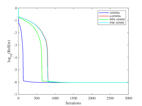
(a)

(b)

(c)

(d)

Figure 1: The change of $\mathrm{log}_{10}(\mathrm{RelErr})$ with the iterations for the tested algorithms under different sparsity rate and rank: (a) spr = 0.05, rank = 10, noiseless; (b) spr = 0.05, rank = 20, noiseless; (c) spr = 0.05, rank = 10, Gaussian noise $\sigma=0.01$; (d) spr = 0.05, rank = 20, Gaussian noise $\sigma=0.01$.

4.3 Nonnegative matrix completion

The original rank-constrained nonnegative matrix completion problem can be formulated as

$$\min_{X\in\mathbb{R}^{m\times n}} \left\|\mathcal{P}_{\Omega}(X-M)\right\|_{F}^{2}$$ (4.5)

$$s.t. rank(X)\leq r,$$

$$X\geq 0,$$

where $M$ is the observation matrix, $r$ is the given upper rank estimation of the matrix $X$, and $\mathcal{P}_{\Omega}$ is the projection onto the sampling set $\Omega$:

$$(\mathcal{P}_{\Omega}(X))_{ij}=\begin{cases}~{}X_{ij},\quad&if~{}(i,j)\in\Omega\\ ~{}0,\quad&if~{}(i,j)\notin\Omega\end{cases}$$

If we reformulate the above problem to a two-block nonconvex optimization problem with a linear equality constraint, either the subproblem is hard to solve, or the reformulated problem has no convergence guarantee. Hence we model the above problem to a three-block nonconvex form as follows.

$$\min_{X,Y,Z\in\mathbb{R}^{m\times n}} \delta_{\mathcal{K}}(X)+\delta_{\mathcal{N}}(Y)+\left\|\mathcal{P}_{\Omega}(Z-M)\right\|_{F}^{2}+\frac{\rho}{2}\|Y-Z\|_{F}^{2}$$ (4.6)

$$s.t. 2X-Y-Z=0,$$

where $\mathcal{K}:=\{X\in\mathbb{R}^{m\times n}:rank(X)\leq r\}$, $\mathcal{N}:=\{X\in\mathbb{R}^{m\times n}:X\geq 0\}$ and $\rho>0$ is the penalty parameter of $\|Y-Z\|_{F}^{2}$. The augmented Lagrangian function of (4.6) is

$$\mathcal{L}_{\beta}(X,Y,Z,\Lambda)=\delta_{\mathcal{K}}(X)+\delta_{\mathcal{N}}(Y)+\left\|\mathcal{P}_{\Omega}(Z-M)\right\|_{F}^{2}+\frac{\rho}{2}\|Y-Z\|_{F}^{2}-\left\langle\Lambda,2X-Y-Z\right\rangle+\frac{\beta}{2}\left\|2X-Y-Z\right\|_{F}^{2}.$$

Note that (4.6) is a form of problem (1.1) with the nonseparable part $H=\frac{\rho}{2}\|Y-Z\|_{F}^{2}$. It has not yet been shown that the algorithms in the first two experiments have convergence guarantees for problems like (4.6). Hence we only apply ADMMn to NMC (4.6), and the update format of ADMMn is

$$(4.7)\quad Y^{k+1}=\frac{1}{\rho+\beta}\max(2\beta X^{k}+(\rho-\beta)Z^{k}-\Lambda^{k},0),$$

$$(4.7)\quad Z^{k+\frac{1}{2}}=(2\Omega\odot M+(\rho-\beta)Y^{k+1}+2\beta X^{k}-\Lambda^{k})\oslash(2\Omega+(\rho+\beta)\textbf{1}),$$

$$(4.7)\quad X^{k+1}=\frac{1}{2}\mathrm{TSVD}(Y^{k+1}+Z^{k+\frac{1}{2}}+\frac{\Lambda^{k}}{\beta},r),$$

$$(4.7)\quad Z^{k+1}=(2\Omega\odot M+(\rho-\beta)Y^{k+1}+2\beta X^{k+1}-\Lambda^{k})\oslash(2\Omega+(\rho+\beta)\textbf{1}),$$

$$(4.7)\quad \Lambda^{k+1}=\Lambda^{k}-\beta(2X^{k+1}-Y^{k+1}-Z^{k+1}),$$

where $\mathrm{TSVD}(\cdot,r)$ is the truncated singular value decomposition (TSVD) [41], and 1 represents the $m\times n$ matrix whose entries all equal to 1.

For comparison, we consider another formulation of (4.5) which is known as the nonnegative factorization matrix completion (NFMC) problem as follows,

$$\operatorname*{min}_{(U,V,X,Y,Z)} \frac{1}{2}\|XY-Z\|_{F}^{2}$$ (4.8)

$$s.t. X=U,Y=V,$$

$$U\geq 0,V\geq 0,$$

$$\mathcal{P}_{\Omega}(Z-M)=0,$$

where $X,U\in\mathbb{R}^{m\times r}$ and $Y,V\in\mathbb{R}^{r\times n}$. An ADMM scheme algorithm is proposed in [7] to solve the five-block problem (4.8) and has the global convergence guarantee. We call it ADM in this experiment and compare our ADMMn with it. Please refer to [7] for more details about the updating format and so on.

Let ’rank’ and ’sr’ represent the rank of the original low-rank matrix $r$ and the sampling rate $|\Omega|/mn$, respectively. The MATLAB code for experiment setup is shown as follows.

⬇

U = rand(m,rank); V = rand(rank,n); X = U*V; % Generate the low-rank matrix

Omega = zeros(m,n); ind = randi(numel(Omega),1,round(m*n*sr));

Omega(ind) = 1; % Generate the sampling set

M = Omega.*X; % The observation matrix

Set $m=n=500$, and test 9 combinations of rank and sampling rate with 20 independently random trials for each combination. For ADMMn on (4.6), set $\rho=1$, $\beta_{1}=1$, and $X$, $Y$, $Z$, $\Lambda$ are all initialized as zero-matrix. To keep consistent with the settings of ADM on (4.8), we set the stopping criterion as

$$\mathrm{RelChg}:=\frac{\|\mathcal{P}_{\Omega}(X^{k}-M)\|_{F}}{\|M\|_{F}}\leq\epsilon\mathrm{~{}or~{}}k>\mathrm{MaxIter},$$

where $\epsilon=10^{-6}$ is the tolerance and $\mathrm{MaxIter}=3000$.

Denote the recovered solution of (4.6) as $(\hat{X},\hat{Y},\hat{Z})$, and the ground truth is $(X^{*},Y^{*},Z^{*})$. We use the following relative error to measure the recovery quality in order to keep consistent with the ADM on (4.8):

$$\mathrm{RelErr}:=\frac{\|\hat{X}-X^{*}\|_{F}}{\|X^{*}\|_{F}+1}.$$

For ADM on (4.8), as [7] suggested, we set $\gamma=1.618$, $\alpha=1.91\times 10^{-4}\|M\|_{F}\frac{\max(m,n)}{r}$ and $\beta_{2}=\frac{n\alpha}{m}$. $U$, $V$, $\Lambda$, $\Pi$ are initialized as zero-matrix, while $Y$ is set as a nonnegative random matrix, and $Z=M$. The stopping criterion in [7] is given as

$$\mathrm{RelChg}:=\frac{\|\mathcal{P}_{\Omega}(X^{k}Y^{k}-M)\|_{F}}{\|M\|_{F}}\leq\epsilon\mathrm{~{}or~{}}k>\mathrm{MaxIter},$$

where $\epsilon=10^{-6}$ is the tolerance and $\mathrm{MaxIter}=3000$.

Denote the recovered solution of (4.8) as $(\hat{X},\hat{Y},\hat{Z},\hat{U},\hat{V})$, and the ground truth is $(X^{*},Y^{*},Z^{*},U^{*},V^{*})$. [7] uses the relative error to measure the recovery quality:

$$\mathrm{RelErr}:=\frac{\|\hat{X}\hat{Y}-X^{*}Y^{*}\|_{F}}{\|X^{*}Y^{*}\|_{F}+1}.$$

Table 4 shows the experiment results. We can see that when the original matrix is really low-rank, both ADMMn and ADM can recover it with high precision, and ADMMn uses much less iterations and time in reconstruction than ADM. However, when the rank of the original matrix is a little large, it can be seen that the recovery quality of ADM is far inferior to ADMMn, and the stopping criterion of ADM is not satisfied in the iterations for this case. Besides, one can find that ADMMn would cost more time than ADM when the number of iterations is the same. This occurs because TSVD is used in NMC (4.6), which is more time-consuming than the matrix factorization in NFMC (4.8). Thanks to the fewer iterations of ADMMn to converge, ADMMn takes less time than ADM in general.

(rank,sr)			ADMMn					ADM
rank	sr		iter	time	RelChg	RelErr		iter	time	RelChg	RelErr
2	0.7		93	0.30	9.4517e-07	1.0523e-06		2833	3.52	9.9568e-06	9.9090e-06
2	0.5		125	0.38	9.6058e-07	1.1160e-06		2806	3.48	1.5677e-05	1.5935e-05
2	0.3		214	0.62	9.6896e-07	1.2213e-06		2966	3.71	3.6358e-05	3.7457e-05
10	0.7		130	0.46	9.4706e-07	1.2106e-06		3000	4.13	3.5762e-04	3.7393e-04
10	0.5		197	0.67	9.6856e-07	1.3378e-06		3000	4.07	7.8137e-04	8.4139e-04
10	0.3		414	1.41	9.8436e-07	1.5899e-06		3000	4.07	4.5016e-04	5.2008e-04
20	0.7		223	1.19	9.6093e-07	1.3835e-06		3000	4.16	2.6131e-03	2.8698e-03
20	0.5		376	2.00	9.7492e-07	1.5764e-06		3000	4.16	2.9042e-03	3.3680e-03
20	0.3		1186	6.29	9.8860e-07	2.0521e-06		3000	4.17	3.3527e-03	4.3619e-03

Table 4: Comparison of the algorithms on NMC / NFMC with different rank and sampling rate.

5 Conclusions

To solve the three-block nonconvex nonseparable problem with linear constraint, we consider an ADMM algorithm with the third variable updated twice in each iteration. With the help of the powerful Kurdyka-Łojasiewicz property, global convergence of the proposed ADMM is established. We also discuss some simple extensions of the proposed ADMM which are useful in practice. At last, we experiment on a recently proposed two-block separable nonconvex MMV problem with $\Psi\equiv 0$, $H\equiv 0$, a three-block separable nonconvex RPCA problem with $H\equiv 0$, and a new three-block nonseparable nonconvex NMC problem proposed by us, respectively. The numerical results show that for the degraded form of (1.1), the proposed ADMM outperforms comparing with others, too. And for (1.1), the proposed ADMM is consistent with theoretical expectations, which also shows a clear advantage in general.

References

- [1] Defeng Sun, Kim-Chuan Toh, and Liuqin Yang. A convergent 3-block semiproximal alternating direction method of multipliers for conic programming with 4-type constraints. SIAM Journal on Optimization, 25(2):882–915, 2015.
- [2] D.L. Donoho. Compressed sensing. IEEE Transactions on Information Theory, 52(4):1289–1306, 2006.
- [3] Yonina C. Eldar and Moshe Mishali. Robust recovery of signals from a structured union of subspaces. IEEE Transactions on Information Theory, 55(11):5302–5316, 2009.
- [4] Zekun Liu and Siwei Yu. Alternating direction method of multipliers based on -norm for multiple measurement vector problem. IEEE Transactions on Signal Processing, 71:3490–3501, 2023.
- [5] Amit Deshpande and Santosh S. Vempala. Adaptive sampling and fast low-rank matrix approximation. Electron. Colloquium Comput. Complex., TR06, 2006.
- [6] Chuangchuang Sun and Ran Dai. A customized admm for rank-constrained optimization problems with approximate formulations. In 2017 IEEE 56th Annual Conference on Decision and Control (CDC), pages 3769–3774, 2017.
- [7] Yangyang Xu, Wotao Yin, Zaiwen Wen, and Yin Zhang. An alternating direction algorithm for matrix completion with nonnegative factors. Frontiers of Mathematics in China, 7:365 – 384, 2011.
- [8] Emmanuel J. Candès, Xiaodong Li, Yi Ma, and John Wright. Robust principal component analysis? J. ACM, 58(3), jun 2011.
- [9] Xiyu Yu, Tongliang Liu, Xinchao Wang, and Dacheng Tao. On compressing deep models by low rank and sparse decomposition. In 2017 IEEE Conference on Computer Vision and Pattern Recognition (CVPR), pages 67–76, 2017.
- [10] Dimitris Bertsimas, Ryan Cory-Wright, and Nicholas A. G. Johnson. Sparse plus low rank matrix decomposition: A discrete optimization approach. Journal of Machine Learning Research, 24(267):1–51, 2023.
- [11] Jim Douglas and H. H. Jr. Rachford. On the numerical solution of heat conduction problems in two and three space variables. Transactions of the American Mathematical Society, 82:421–439, 1956.
- [12] P. L. Lions and B. Mercier. Splitting algorithms for the sum of two nonlinear operators. SIAM Journal on Numerical Analysis, 16(6):964–979, 1979.
- [13] Daniel Gabay and Bertrand Mercier. A dual algorithm for the solution of nonlinear variational problems via finite element approximation. Computers & Mathematics With Applications, 2:17–40, 1976.
- [14] Roland GLOWINSKI and A. Marroco. Sur l’approximation, par elements finis d’ordre un, et la resolution, par penalisation-dualite, d’une classe de problemes de dirichlet non lineaires. Rev Fr Autom Inf Rech Oper, 9(R-2):41–76, 1975.
- [15] Wei Deng and Wotao Yin. On the global and linear convergence of the generalized alternating direction method of multipliers. J. Sci. Comput., 66(3):889–916, mar 2016.
- [16] Bingsheng He and Xiaoming Yuan. On the convergence rate of the douglas–rachford alternating direction method. SIAM Journal on Numerical Analysis, 50(2):700–709, 2012.
- [17] Wei Hong Yang and Deren Han. Linear convergence of the alternating direction method of multipliers for a class of convex optimization problems. SIAM Journal on Numerical Analysis, 54(2):625–640, 2016.
- [18] Roland Glowinski and J. T. Oden. Numerical Methods for Nonlinear Variational Problems. Journal of Applied Mechanics, 52(3):739–740, 09 1985.
- [19] Ke Guo, Deren Han, and Tingting Wu. Convergence of alternating direction method for minimizing sum of two nonconvex functions with linear constraints. International Journal of Computer Mathematics, 94:1653 – 1669, 2017.
- [20] Guoyin Li and Ting Kei Pong. Global convergence of splitting methods for nonconvex composite optimization. SIAM Journal on Optimization, 25(4):2434–2460, 2015.
- [21] Xiang Gao and Shuzhong Zhang. First-order algorithms for convex optimization with nonseparable objective and coupled constraints. Journal of the Operations Research Society of China, 5:131–159, 2017.
- [22] Ke Guo, Deren Han, and Tingting Wu. Convergence of admm for optimization problems with nonseparable nonconvex objective and linear constraints. Pacific Journal of Optimization, 14:489 – 506, 2018.
- [23] Caihua Chen, Bingsheng He, Yinyu Ye, and Xiaoming Yuan. The direct extension of admm for multi-block convex minimization problems is not necessarily convergent. Math. Program., 155(1–2):57–79, jan 2016.
- [24] Deren Han and Xiaoming Yuan. A note on the alternating direction method of multipliers. J. Optim. Theory Appl., 155(1):227–238, oct 2012.
- [25] Ke GUO, Deren HAN, David Z. W. WANG, and Tingting WU. Convergence of admm for multi-block nonconvex separable optimization models. Frontiers of Mathematics in China, 12(5):1139, 2017.
- [26] Fenghui WANG, Wenfei CAO, and Zongben XU. Convergence of multi-blockbregman admm for nonconvex composite problems. SCIENCE CHINA Information Sciences, 61(12):122101–, 2018.
- [27] Chun Zhang, Yongzhong Song, Xingju Cai, and Deren Han. An extended proximal admm algorithm for three-block nonconvex optimization problems. J. Comput. Appl. Math., 398:113681, 2021.
- [28] Mingyi Hong, Zhi-Quan Luo, and Meisam Razaviyayn. Convergence analysis of alternating direction method of multipliers for a family of nonconvex problems. SIAM Journal on Optimization, 26(1):337–364, 2016.
- [29] Yu Wang, Wotao Yin, and Jinshan Zeng. Global convergence of admm in nonconvex nonsmooth optimization. Journal of Scientific Computing, 78:29 – 63, 2015.
- [30] Wen Zaiwen, Hu Jiang, Li Yongfeng, and Liu Haoyang. Optimization: Modeling, Algorithm and Theory(in Chinese). Higher Education Press, 2020.
- [31] R. Tyrrell Rockafellar, Roger J.-B. Wets, and Maria Wets. Variational analysis. In Grundlehren der mathematischen Wissenschaften, 1998.
- [32] Hédy Attouch, Jérôme Bolte, Patrick Redont, and Antoine Soubeyran. Proximal alternating minimization and projection methods for nonconvex problems: An approach based on the kurdyka-Łojasiewicz inequality. Mathematics of Operations Research, 35:438 – 457, 2010.
- [33] Hédy Attouch, Jérôme Bolte, and Benar Fux Svaiter. Convergence of descent methods for semi-algebraic and tame problems: proximal algorithms, forward–backward splitting, and regularized gauss–seidel methods. Mathematical Programming, 137:91–129, 2013.
- [34] Jérôme Bolte, Shoham Sabach, and Marc Teboulle. Proximal alternating linearized minimization for nonconvex and nonsmooth problems. Math. Program., 146(1–2):459–494, aug 2014.
- [35] Yurii Nesterov. Introductory Lectures on Convex Optimization: A Basic Course. Springer Publishing Company, Incorporated, 1 edition, 2014.
- [36] Hédy Attouch and Jérôme Bolte. On the convergence of the proximal algorithm for nonsmooth functions involving analytic features. Mathematical Programming, 116:5–16, 2009.
- [37] Xiaoquan Wang, Hu Shao, Pengjie Liu, and Ting Wu. An inertial proximal partially symmetric admm-based algorithm for linearly constrained multi-block nonconvex optimization problems with applications. J. Comput. Appl. Math., 420(C), mar 2023.
- [38] Jinbao Jian, Pengjie Liu, and Xianzhen Jiang. A partially symmetric regularized alternating direction method of multipliers for nonconvex multi-block optimization. Acta Mathematica Sinica, Chinese Series, 64(6), 2021.
- [39] Ingrid Daubechies, Michel Defrise, and Christine De Mol. An iterative thresholding algorithm for linear inverse problems with a sparsity constraint. Communications on Pure and Applied Mathematics, 57, 2003.
- [40] Zongben Xu, Xiangyu Chang, Fengmin Xu, and Hai Zhang. regularization: A thresholding representation theory and a fast solver. IEEE Transactions on Neural Networks and Learning Systems, 23(7):1013–1027, 2012.
- [41] Tony F. Chan and Per Christian Hansen. Computing truncated singular value decomposition least squares solutions by rank revealing qr-factorizations. SIAM J. Sci. Comput., 11:519–530, 1990.