Continuous Tensor Relaxation for Finding Diverse Solutions
in Combinatorial Optimization Problems

Abstract

Finding the best solution is the most common objective in combinatorial optimization (CO) problems. However, a single solution may not be suitable in practical scenarios, as the objective functions and constraints are only approximations of original real-world situations. To tackle this, finding (i) “heterogeneous solutions”, diverse solutions with distinct characteristics, and (ii) “penalty-diversified solutions”, variations in constraint severity, are natural directions. This strategy provides the flexibility to select a suitable solution during post-processing. However, discovering these diverse solutions is more challenging than identifying a single solution. To overcome this challenge, this study introduces Continual Tensor Relaxation Annealing (CTRA) for unsupervised-learning (UL)-based CO solvers. CTRA addresses various problems simultaneously by extending the continual relaxation approach, which transforms discrete decision variables into continual tensors. This method finds heterogeneous and penalty-diversified solutions through mutual interactions, where the choice of one solution affects the other choices. Numerical experiments show that CTRA enables UL-based solvers to find heterogeneous and penalty-diversified solutions much faster than existing UL-based solvers. Moreover, these experiments reveal that CTRA enhances the exploration ability.

1 Introduction

Combinatorial optimization (CO) problems aim to find the best solution from a discrete space. CO problem is a fundamental problem in many scientific and engineering applications such as transportation logistics, scheduling, network design, and energy management (Glover et al., 2019; Kochenberger et al., 2014; Anthony et al., 2017; Papadimitriou & Steiglitz, 1998; Korte et al., 2011). However, formulating an effective CO problem can be challenging, as real-world issues often involve complex constraints and implicit preferences that are typically simplified in CO formulations. Therefore, obtaining the optimal solution does not necessarily ensure its validity for the original real-world problem. Recently, this issue has attracted increased attention (Fernau et al., 2019; Baste et al., 2022; Hanaka et al., 2023). To tackle this issue, discovering two distinct types of diverse solutions could be a promising way. The first type is “heterogeneous solutions”, which involves finding the set of solutions with distinct characteristics for a CO problems. This diverse solutions enable users to choose a solution, which includes their implicit preferences, during post-processing. The second type is “penalty-diversified solutions”, which involves varying the intensity of constraints by treating them as soft constraints which allows for solutions that may not strictly adhere to the constraints but can violate them with certain penalties. This diverse solutions helps alleviate the problem of overly rigid constraints, where no solutions fully comply, and overly weak constraints that do not model the complexities of real-world problems.

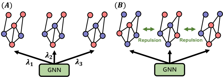
Figure 1: Overview of CRA-PI-GNN solver for penalty-diversified solutions (A) and heterogeneous solutions (B).

Furthermore, the effective exploration of the penalty-diversified solutions would be beneficial for CO solvers based on statistical mechanics, such as adiabatic quantum computation (Albash & Lidar, 2018) and and Fujitsu Digital Annealer (Aramon et al., 2019), as well as for the recently developed unsupervised learning (UL)-based solvers (Wang et al., 2022; Schuetz et al., 2022a; Karalias & Loukas, 2020; Amizadeh et al., 2018). While these solvers are effective for large-scaled CO problems, they can not directly deal with CO problems with hard constraints, which are often essential in practical situation. To address hard-constrained CO problems, these solvers incorporate the constraints into the cost function using penalty method. This method, however, demands considerable computational time to fine-tune the parameters which controls the intensity of incorporated soft constraints; setting the parameter too low might lead to solutions that violate constraints, while setting it too high can complicate the optimization process(Smith et al., 1997). This challenge has emerged as a major bottleneck for the statistical mechanics based and UL based solvers.

To efficiently discover these diverse solutions, this study proposes Continual Tensor Relaxation Annealing (CTRA) method for UL-based CO solvers. CTRA is designed to solve various CO problems in parallel by extending the continual relaxation approach in UL-based solvers, which transforms discrete decision variables into a continual tensor. Through the interaction in UL model, CTRA effectively finds both heterogeneous and penalty-diversified solutions.

Numerical experiments demonstrate that CTRA enables UL-based solvers to find both heterogeneous and penalty-diversified solutions more efficiently than the repetitive use of existing UL-based solvers. The efficient discovery of penalty-diversified solutions considerably reduces the fine-tuning challenges in hard-constrained CO problems using UL-based solvers, which greatly expand the potential for applying UL-based solvers to more complex CO problems. Moreover, the experiments show that exploring heterogeneous solutions with CTRA improve the search capabilities, consequently outperforming existing UL-based solvers.

Notation.

In the following, we use the shorthand expression $[N]=\{1,2,\ldots,N\}$, $N\in{\mathbb{N}}$. $I_{N}\in{\mathbb{R}}^{N\times N}$ represents an identity matrix of size $N\times N$. Here, ${\bm{1}}_{N}$ denotes the vector $(1,\ldots,1)^{\top}\in{\mathbb{R}}^{N}$, and ${\bm{0}}_{N}$ denotes the vector $(0,\ldots,0)^{\top}\in{\mathbb{R}}^{N}$. The matrix $A$ represents the adjacency matrix, where $A_{ij}=0$ indicates no edge between node $i$ and $j$, and $A_{ij}>0$ indicates a weighted edge connecting these nodes. ${\mathbb{V}}{\mathbb{A}}{\mathbb{R}}[\{a_{k}\}_{k=1}^{K}]$ represents the empirical variance $\sum_{k=1}^{K}(a_{k}-\sum_{k^{\prime}=1}^{K}a_{k^{\prime}}/K)^{2}/K$, and ${\mathbb{S}}{\mathbb{T}}{\mathbb{D}}[\{a_{k}\}_{k=1}^{K}]$ denotes the empirical standard deviation $({\mathbb{V}}{\mathbb{A}}{\mathbb{R}}[\{a_{k}\}_{k=1}^{K}])^{1/2}$. For binary vectors ${\bm{a}},{\bm{b}}\in\{0,1\}^{N}$, we define the Hamming distance as $d_{H}({\bm{a}},{\bm{b}})=\sum_{i=1}^{N}{\bm{1}}[a_{i}\neq b_{i}]$, where ${\bm{1}}[\cdot]$ denotes the indicator function.

2 Background

CO Problems.

Our goal is to solve the following constrained CO problem:

$$\min_{{\bm{x}}}f({\bm{x}};C)~{}~{}~{}\mathrm{s.t.}~{}~{}~{}{\bm{x}}\in{\mathcal{X}}(C)$$ (1)

where $C\in{\mathcal{C}}$ represents instance parameters, such as a graph $G=(V,E)$, with $V$ denoting the set of nodes and $E$ the set of edges. The function $f:{\mathcal{X}}\times{\mathcal{C}}\to{\mathbb{R}}$ is the cost function, and the binary vector ${\bm{x}}\in(x_{i})_{1\leq i\leq N}\in\{0,1\}^{N}$ is to be optimized. The feasible solution space ${\mathcal{X}}(C)\subseteq\{0,1\}^{N}$ is typically defined by equality and inequality constraints, as follows:

$${\mathcal{X}}(C)=\{{\bm{x}}\in\{0,1\}^{N}\mid\forall i\in[I],~{}g_{i}({\bm{x}};C)\leq 0,\\ \forall j\in[J],~{}h_{j}({\bm{x}};C)=0\},$$

where, for $i\in[I]$, $g_{i}:\{0,1\}^{n}\times{\mathcal{C}}\to{\mathbb{R}}$ denotes inequality constraints, and for $j\in[J]$, $h_{j}:\{0,1\}^{N}\times{\mathcal{C}}\to{\mathbb{R}}$ denotes equality constraints. These constraints are referred to as “hard constraints”.

Soft Constraint and Penalty Method.

In practical applications, it typically occurs that no solutions completely satisfy all the constraints, or the constraints are not entirely representative of real-world problems. In these cases, considering solutions that slightly violate the constraints to minimize the cost function may be more practical. The penalty method (Smith et al., 1997; Coello, 2002) is used in CO problems for such situations. This method integrates constraints into the cost function as penalties, that is, converting the constrained CO problems as multi-objective CO problems, as follows:

$$\min_{{\bm{x}}}l({\bm{x}};C,{\bm{\lambda}}),~{}~{}l({\bm{x}};C,{\bm{\lambda}})\mathrel{\ensurestackMath{\stackon[1pt]{=}{\scriptstyle\Delta}}}f({\bm{x}};C)+\sum_{i=1}^{I+J}\lambda_{i}v_{i}({\bm{x}};C)$$ (2)

where for all $i\in[I+J]$, $v:\{0,1\}^{N}\times{\mathcal{C}}\to{\mathbb{R}}$ represents a penalty term that increases in value when the constraints are violated. For instance, the penalty term is defined as follows:

$$\forall i\in[I],~{}v_{i}({\bm{x}};C)=\max(0,g_{i}({\bm{x}};C))~{}~{}[\mathrm{Inequality}]$$

$$\forall j\in[J],~{}v_{I+j}({\bm{x}};C)=(h_{j}({\bm{x}};C))^{2}~{}~{}[\mathrm{Equality}]$$

and ${\bm{\lambda}}=(\lambda_{i})_{1\leq i\leq I+J}\in{\mathbb{R}}^{I+J}$ are penalty parameters that balance the trade-off between satisfying the constraints and minimizing the cost function. These integrated constraints are referred to as “soft constraints”. As the penalty parameters ${\bm{\lambda}}$ increase, the severity of the penalty for constraint violations also increases, and vice versa. It can be challenging to predict solutions with specific penalty parameters ${\bm{\lambda}}$ before the optimization process, making it hard to pre-set these parameters to ensure the desired outcome. Therefore, it may be necessary to adjust the penalty parameters during the optimizing process or to find solutions with various penalty parameters.

Moreover, the penalty method is applied to find solutions for CO problems with hard constraints, using statistical mechanics based solvers, such as adiabatic quantum computation (Albash & Lidar, 2018) and and Fujitsu Digital Annealer (Aramon et al., 2019), and UL-based solvers (Wang et al., 2022; Schuetz et al., 2022a; Karalias & Loukas, 2020; Amizadeh et al., 2018), which are incapable of directly addressing hard constraints. In such scenarios, it is essential to adjust the penalty parameters to ensure constraint satisfactions. However, finding a suitable penalty parameters for these solvers is a practical challenge; setting the parameter too low might lead to solutions that violate constraints, while setting it too high can complicate the optimization process (Smith et al., 1997).

Continuous Relaxation and UL-based Solver.

Continuous relaxation is a strategy that converts an original CO problem into a continuous optimization problem. This transformation is typically achieved by converting discrete variables into their continuous counterparts. An example of this approach can be represented as follows:

$$\min_{{\bm{p}}}\hat{l}({\bm{p}};C,{\bm{\lambda}}),~{}~{}\hat{l}({\bm{p}};C,{\bm{\lambda}})\mathrel{\ensurestackMath{\stackon[1pt]{=}{\scriptstyle\Delta}}}\hat{f}({\bm{p}};C)+\sum_{i=1}^{I+J}\lambda_{i}\hat{v}_{i}({\bm{p}};C),$$

where ${\bm{p}}=(p_{i})_{1\leq i\leq N}\in[0,1]^{N}$ represents a set of relaxed continuous variables. Specifically, each binary variable $x_{i}\in\{0,1\}$ is relaxed into a continuous variable $p_{i}\in[0,1]$. $\hat{f}:[0,1]^{N}\times{\mathcal{C}}\to{\mathbb{R}}$ denotes the relaxation of $f$, satisfying $\hat{f}({\bm{x}};C)=f({\bm{x}};C)$ for ${\bm{x}}\in\{0,1\}^{N}$. Similarly, the relationship between the constraint $v_{i}$ and its relaxed counterpart $\hat{v}_{i}$ is maintained for $i\in[I+J]$, i.e., $\forall i\in[I+J],~{}\hat{v}_{i}({\bm{x}};C)=v_{i}({\bm{x}};C)$ for ${\bm{x}}\in\{0,1\}^{N}$.

UL-based solvers use the continuous relaxation strategy (Wang et al., 2022; Schuetz et al., 2022a), designing a machine learning model that outputs a relaxed solution, ${\bm{p}}_{{\bm{\theta}}}(\cdot;C)\in[0,1]^{n}$, parameterized by a neural network with learning parameter ${\bm{\theta}}$. The model is optimized directly through the following objective function:

$$\hat{l}({\bm{\theta}};C,{\bm{\lambda}})\mathrel{\ensurestackMath{\stackon[1pt]{=}{\scriptstyle\Delta}}}\hat{f}({\bm{p}}_{{\bm{\theta}}}(C);C)+\sum_{i=1}^{I+J}\lambda_{i}\hat{v}_{i}({\bm{p}}_{{\bm{\theta}}}(C);C).$$ (3)

In particular, physics-inspired graph neural network (PI-GNN) solver (Schuetz et al., 2022a, b) focuses on CO problems on graphs, denoted as $C=G(V,E)$. This solver employs GNNs to output the relaxed solution, $p_{\theta}(G)$. Specifically, an $L$-layer GNN is designed to minimize $\hat{l}({\bm{\theta}};C,{\bm{\lambda}})$ in Eq. (3). For a more detailed explanation of GNNs, see Appendix B.1. This approach is applicable to cost functions with the following property because it employs a gradient-based algorithm to minimize Eq (3).

Assumption 2.1 (Differentiable cost function).

Throughout the optimization process, both the relaxed cost function $\hat{l}({\bm{\theta}};C,{\bm{\lambda}})$ and its partial derivative $\partial\hat{l}/\partial{\bm{\theta}}$ can be acccessed.

These properties include nonlinear cost functions and multi-body interactions that extent beyond two-body interactions. After training ${\bm{p}}_{\theta}$, the relaxed solution is converted into discrete variables. This conversion can be done by rounding ${\bm{p}}_{\theta}$ as in $\forall i\in[N],~{}x_{i}=\mathrm{int}(p_{\theta,i}(C))$ with a threshold (Schuetz et al., 2022a), a greedy approach (Wang et al., 2022), or by sampling from a Bernoulli distribution with parameter ${\bm{p}}_{\theta}$, as $\forall i\in[N],~{}x_{i}\sim\mathrm{Bernouli}(p_{\theta,i}(C))$.

Although continuous relaxation provides benefits, such as a tractable gradient, it often results in a potential discrepancy between the optimal solutions of the original CO problem and relaxed continuous counterparts. This discrepancy arises as the relaxation expands the solution space. Furthermore, as a CO problem grows more complex, optimizing ${\bm{\theta}}$ becomes more challenging, often hindered by trivial local solutions (Ichikawa, 2023). To mitigate these issues, Ichikawa (2023) has proposed continuous relaxation annealing (CRA) strategy, which includes the following penalty term:

$$\hat{r}({\bm{\theta}};C,{\bm{\lambda}},\gamma)=\hat{l}({\bm{\theta}};C,{\bm{\lambda}})+\phi({\bm{\theta}};C,\gamma,\alpha),\\ \phi({\bm{\theta}};C,\gamma,\alpha)\mathrel{\ensurestackMath{\stackon[1pt]{=}{\scriptstyle\Delta}}}\gamma\sum_{i=1}^{N}(1-(2p_{{\bm{\theta}},i}(C)-1)^{\alpha}),$$ (4)

where $\gamma\in{\mathbb{R}}$ represents a penalty parameter, and an $\alpha$ is an even number in the set $\{2,4,\ldots\}$. Ichikawa (2023) anneals the penalty parameter $\gamma$ in Eq. (4) from negative to positive value, until the penalty term approaches zero, i.e., $\phi({\bm{\theta}},C)\approx 0$. This indicates that the relaxed variables ${\bm{p}}$ are nearly discrete, eliminating the need for artificial rounding from a soft solution to discrete one. Furthermore, this annealing process improves the optimization performance of UL-based solvers. Following Ichikawa (2023), this study adopts a following scheduling, $\gamma(N_{\mathrm{EPOCH}}+1)\leftarrow\gamma(N_{\mathrm{EPOCH}})+\varepsilon$ where $\varepsilon\in{\mathbb{R}}$, a small constant, represents the scheduling rate, and $N_{\mathrm{epoch}}$ denotes the number of updates to the trainable parameter during learning process.

3 Continuous Tensor Relaxation Annealing for UL-based Solver

In this section, we propose the Continual Tensor Relaxation Annealing (CTRA) for UL-based solvers, designed to efficiently solve multiple problems with similar structures simultaneously. Subsequently, we apply the CTRA to the discovery of both penalty-diversified solutions and heterogeneous solutions.

Continuous Tensor Relaxation Strategy.

We consider solving multiple instances $\mathcal{C}_{S}=\{C_{s}\mid C_{s}\in\mathcal{C}\}_{1\leq s\leq S}$, each with different penalty parameters $\Lambda_{S}=\{{\bm{\lambda}}_{s}\}_{1\leq s\leq S}$ simultaneously. To achieve this, we relax a binary vector ${\bm{x}}\in\{0,1\}^{N}$ into an augmented continual tensor $P\in[0,1]^{N\times S}$, and then minimize the following loss function:

$$\hat{R}(P;{\mathcal{C}}_{S},\Lambda_{S},\gamma)=\sum_{s=1}^{S}\hat{l}(P_{:s};C_{s},{\bm{\lambda}}_{s})+\Phi(P;\gamma,\alpha)\\ \Phi(P;\gamma,\alpha)\mathrel{\ensurestackMath{\stackon[1pt]{=}{\scriptstyle\Delta}}}\gamma\sum_{i=1}^{N}\sum_{s=1}^{S}(1-(2P_{is}-1)^{\alpha}),$$ (5)

where $P_{:s}\in[0,1]^{N}$ denotes each column vector of the continuous matrix $P$, i.e. $P=(P_{:s})_{1\leq s\leq S}\in[0,1]^{N\times S}$. When $\hat{R}$ is optimized, each column $P_{:s}$ is to minimize $\hat{l}(P_{:s};C_{s},{\bm{\lambda}}_{s})$. Additionally, we also extend the function $\phi(\cdot)$ in Eq. (4) into $\Phi(\cdot)$ for augmented continual tensor. Specifically, the following theorem holds.

Theorem 3.1.

Under the assumption that the objective function $\sum_{s}\hat{l}(P_{:s};C_{s},{\bm{\lambda}}_{s})$ is bounded within the domain $[0,1]^{N\times S}$, for any $S\in{\mathbb{N}}$, $C_{s}\in{\mathcal{C}}_{S}$ and ${\bm{\lambda}}_{s}\in\Lambda_{S}$, as $\gamma\to+\infty$, each column $P_{:s}^{\ast}$ of the soft solutions, i.e., $P^{\ast}\in\mathrm{argmin}_{P}\hat{R}(P;{\mathcal{C}}_{S},\Lambda_{S},\gamma)$, converges to the original solutions ${\bm{x}}^{\ast}\in\mathrm{argmin}_{{\bm{x}}}l({\bm{x}};C_{s},{\bm{\lambda}}_{s})$. In addition, as $\gamma\to-\infty$, the loss function $\hat{R}(P;{\mathcal{C}}_{S},\Lambda_{S})$ becomes convex and the soft solution ${\bm{1}}_{N}{\bm{1}}_{N}^{\top}/2=\mathrm{argmin}_{P}\hat{R}(P;{\mathcal{C}}_{S},\Lambda_{S},\gamma)$ is unique.

Refer to Appendix A.1 for the detailed proof. The relaxation approach has the potential for further extension to higher-order tensors, exemplified by $P\in[0,1]^{N\times S_{1}\times\cdots}$. Investigating this implementation presents a interesting direction for future research endeavors.

In UL-based solvers, we parameterize the soft tensor solution as follows:

$$\hat{R}({\bm{\theta}};{\mathcal{C}}_{S},\Lambda_{S},\gamma)=\sum_{s=1}^{S}\hat{l}({\bm{\theta}};C_{s},{\bm{\lambda}}_{s})+\Phi({\bm{\theta}};{\mathcal{C}}_{S},\gamma,\alpha)\\ \Phi({\bm{\theta}},{\mathcal{C}}_{S},\gamma,\alpha)\mathrel{\ensurestackMath{\stackon[1pt]{=}{\scriptstyle\Delta}}}\gamma\sum_{i=1}^{N}\sum_{s=1}^{S}(1-(2P_{{\bm{\theta}},is}(C_{s})-1)^{\alpha}).$$ (6)

Following the PI-GNN solver (Schuetz et al., 2022b) and CRA-PI-GNN solver, this study characterizes $P_{\theta}$ using a GNN. Thus, we refer to the PI-GNN applied with CTRA as the “CTRA-PI-GNN” solver. Specifically, the input is a graph $G$ with feature vectors ${\bm{h}}^{(0)}\in{\mathbb{R}}^{H^{(0)}}$ on its nodes. The output of the last layer of the GNN, ${\bm{h}}^{(L)}\in[0,1]^{N\times S}$, on the nodes, represents the soft tensor solution.

Here, both the PI-GNN solver and the CTRA-PI-GNN share the same intermediate layer. The only increase in parameter for the CTRA-PI-GNN solver is in the final layer due to the augmented feature dimension $S$, which induces significant acceleration. This structure is conjectured to learn similar representations up to the final layer for CO problems with similar structures. In Appendix D.2, we provide examples demonstrating the capability of solving multiple problems with similar structures more efficiently and effectively than the CRA-PI-GNN. However, since this paper focuses on acquiring diverse solutions, the extent to which similar problems can be solved quickly remains a topic for future work.

CTRA for Penalty-Diversified Solutions

To finding penalty-diversified solutions, we aim to minimize the following loss function, which is a special case of Eq. (6):

$$\hat{R}({\bm{\theta}};C,\Lambda_{S},\gamma)=\sum_{s=1}^{S}\hat{l}({\bm{\theta}};C,{\bm{\lambda}}_{s})+\gamma\Phi({\bm{\theta}};{\mathcal{C}}_{S},\gamma)$$ (7)

By solving this optimization, each column $P_{\theta,:s}({\mathcal{G}})$ corresponds to the optimal solution for the penalty parameters. ${\bm{\lambda}}_{s}$. Regarding this formulation, we expect that problems differing only their penalty parameters ${\bm{\lambda}}_{s}$ possess multiple similar structures, which allows for the efficient discovery of penalty-diversified solutions.

CTRA for Heterogeneous Solutions.

Next, for the exploration of heterogeneous solutions, we introduce a diversity metric of solutions in Eq. (6). Specifically, we aim to minimize the following loss function:

$$\hat{R}({\bm{\theta}};C,{\bm{\lambda}},\gamma)+\Psi({\bm{\theta}};C,\nu),\\ \Psi({\bm{\theta}};C,\nu)=-\nu S\sum_{i=1}^{N}{\mathbb{S}}{\mathbb{T}}{\mathbb{D}}\left[\{P_{{\bm{\theta}},is}(C)\}_{1\leq s\leq S}\right],$$ (8)

where, $\Psi({\bm{\theta}};C,\nu)$ acts as a constraint term to induce diversity in each column $P_{\theta,:s}(C)$, and $\nu$ is the parameter controlling the intensity of this constraints. Setting $\nu$ to $0$ in Eq. (8) almost corresponds to tackling the same CO problem with different initial conditions. Additionally, the following proposition indicate that this diversity measure $\Psi({\bm{\theta}};C,\nu)$ is a natural relaxation of the diversity metric in CO problems, known to max sum hamming distance (Fomin et al., 2020, 2023; Baste et al., 2022, 2019).

Proposition 3.2.

For the binary sequence $\{{\bm{x}}_{s}\}_{s=1}^{S}$, $\forall s\in[S],{\bm{x}}_{s}\in\{0,1\}^{N}$, following equality holds

$$S^{2}\sum_{i=1}^{N}{\mathbb{V}}{\mathbb{A}}{\mathbb{R}}\left[\{{\bm{x}}_{s,i}\}_{1\leq s\leq S}\right]=\sum_{s<l}d_{H}({\bm{x}}_{s},{\bm{x}}_{l}).$$ (9)

where the right-hand side of Eq. (9) is the max sum hamming distance.

Refer to Appendix A.2 for the detailed proof. This proposition indicate for a continuas tensor variable $P\in[0,1]^{N\times S}$, the variance in the left-hand side of Eq.(9) is the relaxation of max sum hamming distance. This study use standard deviation in Eq. 8 to match scaling of other terms in Eq. 8.

4 Experiments

This section evaluate the effectiveness of CTRA-PI-GNN solver in identifying penalty-diversified and heterogeneous solutions across three CO problems. First, we briefly describe the experimental settings.

4.1 Settings

Maximum Independent Set Problems.

The MIS problem, a fundamental NP-hard problem (Karp, 2010), has various applications in the network design (Hale, 1980) and finance (Boginski et al., 2005) fields. Given an undirected graph $G(V,E)$, the MIS problem aims to find the largest independent set, wherein no two nodes are adjacent. The problem formulation assigns a binary variable $x_{i}$ to each node $i\in V$, where the MIS problem is identical to maximizing the number of nodes assigned $1$ while ensuring that their non-adjacency. Specifically, it is formulated as minimizing:

$$l({\bm{x}};G,\lambda)=-\sum_{i\in V}x_{i}+\lambda\sum_{(i,j)\in E}x_{i}x_{j},$$ (10)

where the first term aims to maximize the number of nodes assigned $1$, while the second term impose penalties on the adjacent nodes marked $1$. This experiments adopt the MIS problems on random-regular graphs (RRG), as in UL-based solvers due to the difficulty (Schuetz et al., 2022a; Wang & Li, 2023); see Appendix C.1.1 for the detailed theoretical background. Consistent with Schuetz et al. (2022a); Wang & Li (2023), this experiments use RRG with the node degree $d=3,5,20$, where $d=20$ is the hardest setting, see Appendix C.1.1 for the background.

Diverse Bipartite Matching (DBM) Problems.

We adopt this CO problem from Ferber et al. (2020); Mulamba et al. (2020); Mandi et al. (2022) as a practical example. The topologies are sourced from the CORA citation network (Sen et al., 2008), where each node signifying a scientific publication, is characterized by $1{,}433$ bag-of-words features, and the edges represents represents the likelihood of citation links. Mandi et al. (2022) focused on disjoint topologies, creating $27$ distinct instances. Each instance is composed of $100$ nodes, categorised into two group of $50$ nodes, labeled $N_{1}$ and $N_{2}$. The objective of DBM problems is to find the maximum matching under diversity constraints for similar and different fields. It is formulated as follows:

$$\begin{split}&l({\bm{x}};C,M,{\bm{\lambda}})=-\textstyle\sum_{ij}C_{ij}x_{ij}\\ &\qquad+\lambda_{1}\textstyle\sum_{i=1}^{N_{1}}\mathrm{ReLU}\Big{(}\textstyle\sum_{j=1}^{N_{2}}x_{ij}-1\Big{)}\\ &\qquad+\lambda_{2}\textstyle\sum_{j=1}^{N_{2}}\mathrm{ReLU}\Big{(}\textstyle\sum_{i=1}^{N_{1}}x_{ij}-1\Big{)}\\ &\qquad+\lambda_{3}\mathrm{ReLU}\Big{(}p\textstyle\sum_{ij}x_{ij}-\textstyle\sum_{ij}M_{ij}x_{ij}\Big{)}\\ &\qquad+\lambda_{4}\mathrm{ReLU}\Big{(}q\textstyle\sum_{ij}x_{ij}-\textstyle\sum_{ij}(1-M_{ij})x_{ij}\Big{)},\end{split}$$ (11)

where a reward matrix $C\in{\mathbb{R}}^{N_{1}\times N_{2}}$ indicates the likelihood of a link between each node pair, for all $i,j$, $M_{ij}$ is assigned $0$ if articles $i$ and $j$ belong to the same field, or $1$ if they don’t. The parameters $p,q\in[0,1]$ represent the probability of pairs being in the same field and in different fields, respectively. Following (Mandi et al., 2022), we examine two variations of this problem: Matching-1 and Matching-2, characterized by $p$ and $q$ values of $25$% and $5$%.

Maximum Cut Problems.

The MaxCut problem, a well-known NP hard problems (Karp, 2010), has practical application in machine scheduling (Alidaee et al., 1994), image recognition (Neven et al., 2008) and electronic circuit layout design (Deza & Laurent, 1994). It is defined as follows: In an undirected graph $G=(V,E)$, a cut set ${\mathcal{C}}\in E$, which is a subset of edges, divides the nodes into two groups $(V_{1},V_{2}\mid V_{1}\cup V_{2}=V,~{}V_{1}\cap V_{2}=\emptyset)$. The objective the MaxCut problem is to find the largest cut set. To formulate this problem, each node is assigned a binary variable: $x_{i}=1$ signifies that node $i$ is in $V_{1}$, while $x_{i}=0$ indicates node $i$ is in $V_{2}$. For an edge $(i,j)$, $x_{i}+x_{j}-2x_{i}x_{j}=1$ is true if $(i,j)\in{\mathcal{C}}$; otherwise, it equal $0$. This leads to the following objective function:

$$l({\bm{x}};G)=\sum_{i<j}A_{ij}(2x_{i}x_{j}-x_{i}-x_{j})$$ (12)

where $A_{ij}$ is the adjacency matrix, where $A_{ij}=0$ signifies the absence of an edge, and $A_{ij}>0$ indicates a connecting edge. Following Schuetz et al. (2022a); Ichikawa (2023), this experiments employ seven instances from Gset dataset (Ye, 2003), recognized as a standard MaxCut benchmark. These seven instances are defined on distinct graphs, including Erdös-Renyi graphs with uniform edge probability, graphs with gradually decaying connectivity from $1$ to $N$, 4-regular toroidal graphs, and one of the largest instance with $10{,}000$ nodes.

Baseline.

In all experiments, we take CRA-PI-GNN solver Ichikawa (2023) as the direct baseline method. For the MaxCut problems, we also include the PI-GNN solver Schuetz et al. (2022a) and the RUN-CSP solver (Toenshoff et al., 2019) as additional baselines. We track the time $t$ that the model learns and then outputs solutions. Note that we do not consider UL-based solvers because they generally perform worse than the CRA-PI-GNN and RUN-CSP solvers. We also do not include UL-based solvers that use historical information (Karalias & Loukas, 2020; Wang & Li, 2023), focusing on the case where historical information is not utilized.

Implementation.

The main objective of our numerical experiments is to conduct a comparative analysis between the CTRA-PI-GNN and CRA-PI-GNN solvers. Thus, we follow the experimental settings in (Schuetz et al., 2022a, 2023; Ichikawa, 2023), where a simple GraphSAGE (Hamilton et al., 2017) architecture with PyTorch GraphSage implemented using the Deep Graph Library (Wang et al., 2019). For each node $v\in V$, the first convolutional layer takes a node embedding vectors, ${\bm{h}}_{v,{\bm{\theta}}}^{(0)}$ for each node, yielding feature vectors ${\bm{h}}_{v,{\bm{\theta}}}^{(1)}\in{\mathbb{R}}^{H^{(1)}}$. Then, the ReLU function is used as a component-wise nonlinear transformation. The second convolutional layer takes the feature vector, ${\bm{h}}^{(1)}_{{\bm{\theta}}}$, as input, producing a feature vector ${\bm{h}}^{(2)}_{v,{\bm{\theta}}}\in{\mathbb{R}}^{S}$. Finally, a sigmoid function is applied to the vector ${\bm{h}}^{(2)}_{{\bm{\theta}}}$, producing the tensor solutions $P_{v:,{\bm{\theta}}}\in[0,1]^{N\times S}$. Here, for MIS and MaxCut problems, we set $H^{(0)}$ as $\mathrm{int}(N^{0.8})$ as in Schuetz et al. (2022a); Ichikawa (2023), and for the DBM problems, we set it to $2{,}500$. Across all problems, we set $H^{(1)}=H^{(0)}$, and $H_{2}=S$. We use the AdamW (Kingma & Ba, 2014) optimizer with a learning rate as $\eta=10^{-4}$ and weight decay as $10^{-2}$. The training the GNNs conducted for a duration of up to $5\times 10^{4}$ epochs with early stopping, which monitors the summarized loss function $\sum_{s=1}^{S}\hat{l}(P_{:,s})$ and penalty term $\Phi(P;\gamma,\alpha)$ with tolerance $10^{-5}$ and patience $10^{3}$. Lastly, we set the initial scheduling value as $\gamma(0)=-20$ for the MIS and DBM problems and $\gamma(0)=-6$ for the MaxCut problems, with same scheduling rate $\varepsilon=10^{-3}$ and curveture rate $\alpha=2$ in Eq. (6). After the training phase, we apply projection heuristics to round the obtained soft solutions back to discrete solutions using simple projection, where for all $i\in[N],s\in[S]$, we map $P_{\theta,i,s}$ to $0$ if $P_{\theta,i,s}\leq 0.5$ and $P_{\theta,i,s}$ to $1$ if $P_{\theta,i,s}>0.5$. Due to the early stopping, the CRA-PI-GNN solver ensures that the soft solution are nearly binary for all benchmarks, making them robust against the threshold $0.5$ in our experiments.

Evaluation Metric

Following the metric of Wang & Li (2023), we adopt the approximation rate (ApR) for the MIS problems, defined by $\mathrm{ApR}=f({\bm{x}};C)/f({\bm{x}}^{\ast})$, where ${\bm{x}}^{\ast}$ signifies the theoretical results (Barbier et al., 2013). All the results for MIS are summarized based on 5 RRGs with different random seeds. For the DBM problems, we calculate the ApR against the global optimal, which is identified using Gurobi 10.0.1 solver with default settings. For the MaxCut Gset problem, the ApR is assessed relative to the best-known solutions.

4.2 Finding penalty-diversified Solutions

In this section, we demonstrate that CTRA-PI-GNN solver can discover penalty-diversified solutions much faster than by running the CRA-PI-GNN solver on multiple times.

MIS Problems.

First, we conduct a comparison between the CTRA-PI-GNN and CRA-PI-GNN solvers for the MIS problems on RRGs $G(V,E)$ with the node $10{,}000$ nodes and the node degree selected as $5$ and $20$. We run CTRA-PI-GNN solver using Eq. 7, employing a set of penalty parameters, $\Lambda_{S}=\{2^{s-3}\mid s=1,\ldots,20\}$. In contrast, the CRA-PI-GNN solver is run multiple times for each distinct $\lambda_{s}\in\Lambda_{S}$.

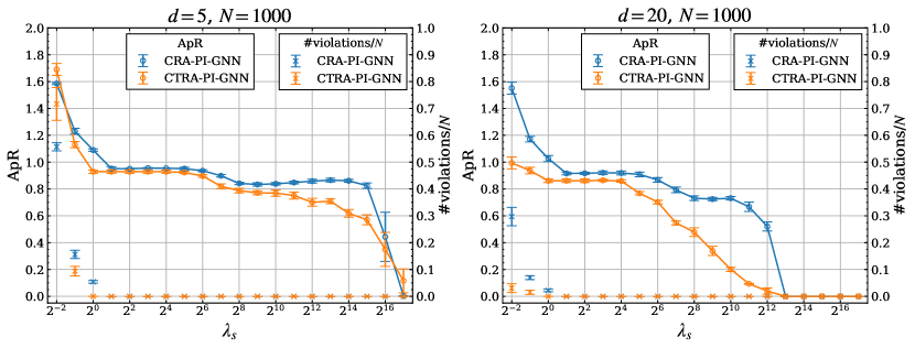
Figure 2: The ApR of MIS problems on RRGs with $10{,}000$ nodes as a function of the penalty parameters $\Lambda_{S}$, using both the CTRA-PI-GNN and CRA-PI-GNN solvers. (Left) Results for graphs with the node degree $d=5$. (Right) Results for graphs with the node degree $d=20$. Error bars represent the standard deviations of 5 random seeds.

Figure 2 shows the ApR as a function of penalty parameters $\Lambda_{s}$, using CTRA-PI-GNN and CRA-PI-GNN solver. Across all penalty parameters, from $2^{-2}$ to $2^{17}$, the CTRA-PI-GNN solver performs on par with or slightly underperforms the CRA-PI-GNN solver, whose underperformance is in the region from $\lambda_{s}\in\{2^{5},2^{12}\}$ on the graphs with the degree $d=20$. Next, we investigate how the runtime of the CTRA-PI-GNN solver is influenced by the number of shots, $S$, compared to the runtime for $S$ individual runs of the PI-GNN solver. Figure 3 shows each runtime as a function of the number of shots $S$. For this analysis, we incrementally increase the number of shots, further dividing the range of penalty parameters from $2^{-2}$ to $2^{17}$. The results indicate that the CTRA-PI-GNN solver can find penalty-diversified solutions within a runtime nearly identical to that of a single run of the CRA-PI-GNN solver for shot numbers $S$ from $2^{0}$ to $2^{9}$. However, for $S>2^{9}$, we observe a linear increase in runtime as the number of shots $S$ grows.

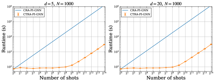
Figure 3: The runtime of the CTRA-PI-GNN solver, compared to $S$ individual runs of the CRA-PI-GNN solver, as a function of number of shots $S$. Error bars represent the standard deviations of 5 random seeds.

As a result, the CTRA-PI-GNN solver efficiently finds penalty-diversified solutions, mitigating the bottleneck issue of penalty parameter tuning in UL-based solvers.

DBM Problems.

Next, we demonstrate that the CTRA-PI-GNN solver can efficiently find the penalty-diversified solutions in DBM problems, which serve as practical CO problems. We focus on the first of 27 DBM instances; see Appendix D.3 for the results of other instances except for the first. Since $(\lambda_{1},\lambda_{2})$ and $(\lambda_{3},\lambda_{4})$ would have the same properties, we run the CTRA-PI-GNN for $S=11\times 11$ shots on the a grid, $\Lambda_{S}=\{{\bm{\lambda}}_{s}=(\lambda_{a},\lambda_{a},\lambda_{b},\lambda_{b})\}$, where $\lambda_{a},\lambda_{b}\in\{2^{s}\mid s=0,\ldots,10\}$. In comparison, the CRA-PI-GNN solver is executed multiple times for each ${\bm{\lambda}}_{s}\in\Lambda_{S}$. Figure 4 shows the ApR across the grid $\lambda_{S}$ using the CTRA-PI-GNN solver. Furthermore, the CTRA-PI-GNN solver demonstrates a significant reduction in runtime, $1{,}961\pm 101$ seconds, compared to the cumulative runtime of executing the CRA-PI-GNN solver $11\times 11$ times, $165{,}291\pm 2{,}851$ seconds. These results indicate that the CTRA-PI-GNN solver can explore both the optimal ${\bm{\lambda}}_{s}$ where the ApR equals one and the regions causing constraint violations all within a significantly reduced runtime compared to the CRA-PI-GNN solver.

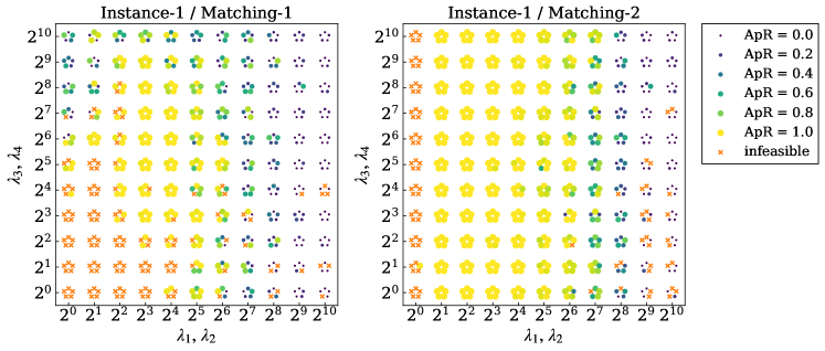
Figure 4: The ApR for the DBM problems across the grid $\Lambda_{S}$ using CTRA-PI-GNN solver. (left) Results for Matching-$1$ where $p=q=25$%. (right) Results for the matching- $2$ where $p=q=5$%. Each point on the coordinate plane represents the results with five different random seed, with the colors indicating the ApR. The constraints violations are marked with a cross symbol.

4.3 Finding Heterogeneous Solutions

Next, we demonstrate that the CTRA-PI-GNN solver can find heterogeneous solutions and enhance the exploration.

MIS Problems.

We first run CTRA-PI-GNN solver using Eq. (8) to find heterogeneous solutions for MIS problems on small-scaled RRGs with $30$ nodes and the node degree set to $3$. We set the parameter $\nu=0.5$ and the number of shots $S=100$ in Eq. (8). As shown in Figure 5, CTRA-PI-GNN solver can successfully obtain $6$ solutions with $13$ independent sets, which is the global optimum value.

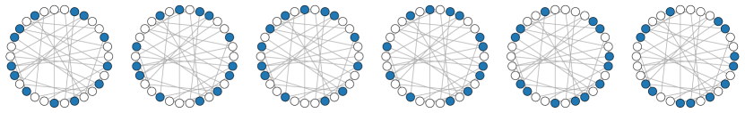
Figure 5: The obtained solutions by CTRA-PI-GNN solver for the MIS problem on a RRG with $30$ nodes and the degree $d=3$. Blue nodes represent the independent set.

We extend the investigation to large-scale RRG with $10{,}000$ nodes and a node degree $d=20$, which is known for its optimization challenges (Angelini & Ricci-Tersenghi, 2023). Particularly, these experiments examine the parameter $\nu$ dependency with a fixed number of shots $S=300$. Figure 6 (left) shows the distribution of hamming distances combination, $\{d_{H}(P_{:s},P_{:l})\}_{1\leq s<l\leq 300}$, and the count of unique solutions with different $\nu=0.00,0.05,0.10,0.20$, whereas Figure 6 (right) shows the maximum ApR, i.e., $\max_{s=1,\ldots,300}\mathrm{ApR}(P_{:,s})$ as a function of the parameter $\nu$. These results indicate that the CTRA-PI-GNN solver can find more heterogeneous solutions as the parameter $\nu$ increases. Furthermore, This result indicates that the CTRA-PI-GNN solver can boost the exploration capabilities of the CRA-PI-GNN solver, leading to the discovery of better solutions.

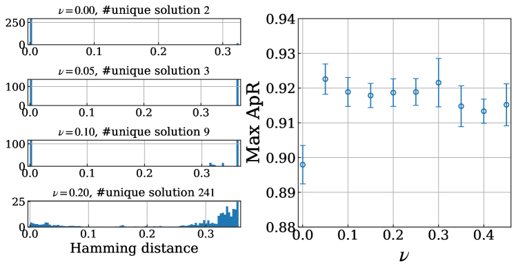
Figure 6: The density of Hamming distance combination of the solution, $\{d_{H}(P_{:s},P_{:l})\}_{1\leq s<l\leq 300}$, with different parameters $\nu$ and the count of unique solutions (left), and the maximum ApR, $\max_{s=1,\ldots,300}\mathrm{ApR}(P_{:s})$, as a function of the parameter $\nu$.

MaxCut Problem.

Next, we examine the performance of the CTRA-PI-GNN solver on the MaxCut benchmark instances within the Gset. We first evaluate the ability to find heterogeneous solutions in the G14 instance, which has 4-clustered solution space. For this analysis, we set the number of shot $S=1{,}000$ in Eq. (8). Figure 7 (left) illustrates that a 2 dimensional mapping of solutions $\{P_{:s}\}_{s=1}^{1000}$ using principal component analysis, selecting the two principal components with the highest contribution rates for different parameters $\nu=0.0,0.4,0.8,1.2$. 7 show the ApR as a function of the parameter $\nu$; see Appendix D.1 for the distribution of hamming distance combination, $\{d_{H}(P_{:s},P_{:l})\}_{1\leq s<l\leq 1{,}000}$. These results shows that, by adjusting $\nu$, the CTRA-PI-GNN solver not only discovers 4-clustered solutions but also enhance the exploration of the CRA-PI-GNN solvers. These improvement is consistent across other Gset instances on distict graphs with varying nodes, as shown in Table. 1. In these experiment, we fix as $\nu=6$ and evaluate the maximum ApR, $\max_{s=1,\ldots,1000}\mathrm{ApR}(P_{:s})$. This result shows that CTRA-PI-GNN solver outperforme CRA-PI-GNN, PI-GNN, and RUN-CSP solvers.

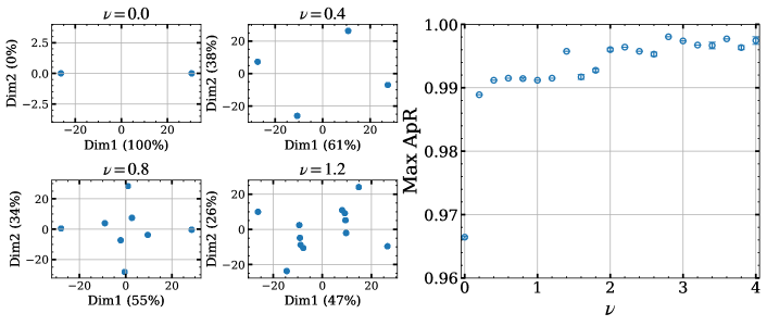
Figure 7: (Left) the 2-dimension mapping by first and second principal components of the solutions generated by the CTRA-PI-GNN solvers with different parameters $\nu$. (Right) The maximum ApR, $\max_{s}\mathrm{ApR}(P_{:s})$ with error bars indicating the standard deviations of 5 random seeds.

Table 1: Numerical results for MaxCut on Gset instances

(Nodes, Edges)	CSP	PI	CRA	CTRA
G14 ($800$, $4{,}694$)	$0.960$	$0.988$	$0.994$	$0.997$
G15 ($800$, $4{,}661$)	$0.960$	$0.980$	$0.992$	$0.995$
G22 ($2{,}000$, $19{,}990$)	$0.975$	$0.987$	$0.998$	$0.999$
G49 ($3{,}000$, $6{,}000$)	$\mathbf{1.000}$	$0.986$	$\mathbf{1.000}$	$\mathbf{1.000}$
G50 ($3{,}000$, $6{,}000$)	$\mathbf{1.000}$	$0.990$	$\mathbf{1.000}$	$\mathbf{1.000}$
G55 ($5{,}000$, $12{,}468$)	$0.982$	$0.983$	$0.991$	$0.994$
G70 ($10{,}000$, $9{,}999$)	$-$	$0.982$	$0.992$	$0.997$

5 Related Work

In the following, we review two groups of works: UL-based solvers for CO optimization and exploration of diverse solutions.

UL-based Solvers.

UL-based solvers have attracted attention in CO problems (Cappart et al., 2023; Lamb et al., 2020). Previous works of UL-based solver have studied constraint satisfaction problems (Toenshoff et al., 2019; Amizadeh et al., 2018) and TSP problems (Hudson et al., 2021) , while these works depend on carefully designed cost function. Employing these approaches to address general CO problems necessitates problem reductions. Karalias & Loukas (2020) propose an UL-solver for general CO problems based on the Erdős’ probabilistic method. Wang et al. (2022) generalize this UL-solver and prove that if the CO cost function can be relaxed into an entry-wise concave form, a solution of good quality can be achieved. Schuetz et al. (2022a, b) have recently extend this UL-based solver (Karalias & Loukas, 2020) to large scale CO problems. Furthermore, (Wang & Li, 2023) have applied meta learning to UL-based solver using historical instances and the solutions and pointed out that PI-GNN solver does not learn from history but is directly optimized over each instance, which tends to be trapped into a local optimum and then is inferior to the greedy algorithms. As in (Wang & Li, 2023), while the PI-GNN solver struggles with optimization issues, discussed in Sec., CRA approach achieves outperforms the greedy algorithms.

Exploration of Diverse Solutions.

Recently, finding diverse solutions in CO problems have attracted increasing attention in many fields (Fernau et al., 2019; Baste et al., 2019, 2022). Previous studies typically employ a diversity measure based on Hamming distance to evaluate the diversity of solutions (Fomin et al., 2020, 2023). These studies consider the problem of finding diverse solutions as a multi-objective optimization problem, simultaneously optimizing the cost function and these diversity measures. In particular, these methods are applied for methods such as mathematical programming (Danna et al., 2007; Danna & Woodruff, 2009; Petit & Trapp, 2019), constraint programming (Hebrard et al., 2005; Petit & Trapp, 2015), and heuristics (Drosou & Pitoura, 2010; Van Hentenryck et al., 2009; Vieira et al., 2011). Additionally, the theoretical aspects of the problems finding diverse solutions have been investigated (Fernau et al., 2019), revealing that finding diverse solutions is much harder than finding a single solution. This theoretical study has also developed the algorithms for finding diverse solutions (Baste et al., 2019, 2022), which have been applied for specific CO problems (Hanaka et al., 2021; Fomin et al., 2020); However, these methods encounter the challenge of a limited number of solutions that can be found, which can be a potential bottleneck in practice. However, CTRA-PI-GNN solvers can find relatively large diverse solutions.

6 Conclusion

In CO problems, the objective functions and constraints typically approximate the original real-world situations. In such cases, exploring heterogeneous and penalty-diversified solutions is essential, as they provide the flexibility to select an appropriate solution, adopting the complexities and uncertainties inherent in real-world situations. We introduced the Continual Tensor Relaxation Annealing (CTRA) method for UL-based solvers to address these diverse solutions. CTRA efficiently finds these diverse solutions much faster than existing approaches. Furthermore, this approach addresses the limitations of tuning the penalty parameters in UL-based solvers when dealing with hard constraints.

Appendix A Derivations

A.1 Proof of Theorem 3.1

Following the proof of Ichikawa (2023), we show Theorem A.4 based on following three lemmas.

Lemma A.1.

For any even natural number $\alpha=2,4,\ldots$, the function $\phi(p;\alpha)=1-(2p-1)^{\alpha}$ defined on $[0,1]$ achieves its maximum value of $1$ when $p=1/2$ and its minimum value of $0$ when $p=0$ or $p=1$.

Proof.

The derivative of $\phi(p;\alpha)$ relative to $p$ is $\phi^{\prime}(p;\alpha)=-2\alpha(2p-1)$, which is zero when $p=1/2$. This is a point where the function is maximized because the second derivative $\phi^{\prime\prime}(p;\alpha)=-4\alpha\leq 0$. In addition, this function is concave and symmetric relative to $p=1/2$ because $\alpha$ is an even natural number, i.e., $\phi(p;\alpha)=\phi(1-p;\alpha)$, thereby achieving its minimum value of $0$ when $p=0$ or $p=1$. ∎

Lemma A.2.

For any even natural number $\alpha=2,4,\ldots$ and a matrix $P\in[0,1]^{N\times S}$, if $\lambda\to+\infty$, minimizing the penalty term $\Phi(P;\gamma,\alpha)=\gamma\sum_{s=1}^{S}\sum_{i=1}^{N}(1-(2P_{is}-1)^{\alpha})=\gamma\sum_{s=1}^{S}\sum_{i=1}^{N}\phi(P_{is};\alpha)$ enforces that the components of $P_{is}$ must be either $0$ or $1$ and, if $\gamma\to-\infty$, the penalty term enforces $P={\bm{1}}_{N}{\bm{1}}_{N}^{\top}/2$.

Proof.

From Lemma B1, as $\gamma\to+\infty$, the case where $\phi(P_{is};\alpha)$ becomes minimal occurs when, for each $i,s$, $p_{is}=0$ or $p_{i}=1$. In addition, as $\gamma\to-\infty$, the case where $\phi(p;\alpha,\gamma)$ is minimized occurs when, for each $i$, $P_{is}$ reaches its maximum value with $P_{is}=1/2$. ∎

Lemma A.3.

$\Phi(P;\gamma,\alpha)=\gamma\sum_{s=1}^{S}\sum_{i=1}^{N}(1-(2p_{i}-1)^{\alpha})=\gamma\sum_{s=1}^{S}\sum_{i=1}^{N}\phi(p_{i};\alpha)$ is concave when $\lambda$ is positive and is a convex function when $\lambda$ is negative.

Proof.

Note that $\Phi(P;\gamma,\alpha)=\gamma\sum_{s=1}^{S}\sum_{i=1}^{N}\phi(P_{is};\alpha)=\gamma\sum_{i=1}^{N}(1-(2P_{is}-1)^{\alpha})$ is separable across its components $P_{is}$. Thus, it is sufficient to prove that each $\gamma\phi(P_{is};\alpha)$ is concave or convex in $P_{is}$ because the sum of the concave or convex functions is also concave (and vice versa). Therefore, we consider the second derivative of $\gamma\phi_{i}(P_{is};\alpha)$ with respect to $P_{is}$:

$$\gamma\frac{d^{2}\phi_{i}(P_{is};\alpha)}{dP_{is}^{2}}=-4\gamma\alpha$$

Here, if $\gamma>0$, the second derivative is negative for all $p_{i}\in[0,1]$, and this completes the proof that $\Phi(P;\gamma,\alpha)$ is a concave function when $\gamma$ is positive over the domain ${\bm{p}}\in[0,1]^{N}$ ∎

Theorem A.4.

Under the assumption that the objective function $\sum_{s}\hat{l}(P_{:s};C_{s},{\bm{\lambda}}_{s})$ is bounded within the domain $[0,1]^{N\times S}$, for any $S\in{\mathbb{N}}$, $C_{s}\in{\mathcal{C}}_{S}$ and ${\bm{\lambda}}_{s}\in\Lambda_{S}$, as $\gamma\to+\infty$, each column $P_{:s}^{\ast}$ of the soft solutions $P^{\ast}\in\mathrm{argmin}_{P}\hat{R}(P;{\mathcal{C}}_{S},\Lambda_{S},\gamma)$ converges to the original solutions ${\bm{x}}^{\ast}\in\mathrm{argmin}_{{\bm{x}}}l({\bm{x}};C_{s},{\bm{\lambda}}_{s})$. In addition, as $\gamma\to-\infty$, the loss function $\hat{R}(P;{\mathcal{C}}_{S},\Lambda_{S})$ becomes convex and the soft solution ${\bm{1}}_{N}{\bm{1}}_{N}^{\top}/2=\mathrm{argmin}_{P}\hat{R}(P;{\mathcal{C}}_{S},\Lambda_{S},\gamma)$ is unique.

Proof.

As $\lambda\to+\infty$, the penalty term $\Phi(P;\alpha)$ dominates the loss function $\hat{R}({\bm{p}};C,{\bm{\lambda}},\gamma)$. According to Lemma B.2, this penalty term forces the optimal solution $P^{\ast}$ to have components $p_{is}^{\ast}$ that are either $0$ or $1$ because any nonbinary value will result in an infinitely large penalty. This effectively restricts the feasible region to the vertices of the unit hypercube, which correspond to the binary vector in $\{0,1\}^{NS}$. Thus, as $\lambda\to+\infty$, the solutions to the relaxed problem converge to $X=\mathrm{argmin}_{X\in\{0,1\}^{N\times S}}R(X_{:s};C_{s},{\bm{\lambda}}_{s})$. Futhermore, $\mathrm{argmin}_{X\in\{0,1\}^{N\times S}}R(X_{:s};C_{s},{\bm{\lambda}}_{s})$ is separable as $\sum_{s=1}^{S}\mathrm{argmin}_{{\bm{x}}\in\{0,1\}^{N}}l({\bm{x}};C_{s},{\bm{\lambda}}_{s})$, which indicate that each columns $X_{:s}^{\ast}\in\mathrm{argmin}_{{\bm{x}}\in\{0,1\}^{N}}l({\bm{x}};C_{s},{\bm{\lambda}}_{s})$. As $\lambda\to-\infty$, the penalty term $\Phi({\bm{p}};\alpha)$ also dominates the loss function $\hat{r}({\bm{p}};C,{\bm{\lambda}},\gamma)$ and the $\hat{r}({\bm{p}};C,{\bm{\lambda}})$ convex function from Lemma B.3. According to Lemma B.2, this penalty term forces the optimal solution $P^{\ast}={\bm{1}}_{N}{\bm{1}}_{N}/2$. ∎

A.2 Proof of Proposition 3.2

In this section, we derive Eq. (9) in Proposition 3.2. optimization.

Proof.

We first note that, for binary vectors ${\bm{x}}_{s},{\bm{x}}_{l}\in\{0,1\}^{N}$, the Hamming distance is expressed as follows:

$$d_{H}({\bm{x}}_{s},{\bm{x}}_{l})=\sum_{i=1}^{N}\left(x_{s,i}^{2}+x_{l,i}^{2}-2x_{s,i}x_{l,i}\right).$$ (13)

Based on this expression, the diversity metric $\sum_{s<l}d_{H}(X_{:s},X_{:l})$ can be expanded for a binary matrix $X\in\{0,1\}^{N\times S}$ as follows:

$$\sum_{s<l}d_{H}(X_{:s},X_{:l}) =\frac{1}{2}\left(\sum_{sl}d_{H}(X_{:s},X_{:l})-\sum_{s}d_{H}^{2}(X_{:s},X_{:s})\right)$$

$$=\frac{1}{2}\sum_{i=1}^{N}\sum_{sl}(X_{:s,i}^{2}+X_{:l,i}^{2}-2X_{:s,i}X_{:l,i})$$

$$=S\sum_{i}^{N}\left(\sum_{s}X_{:s,i}^{2}-\frac{1}{S}\sum_{s,l}X_{:s,i}X_{:l,i}\right).$$

On the other hand, the variance of each column in a binary matrix $X$ can be expanded as follows:

$$S^{2}\sum_{i=1}^{N}{\mathbb{V}}{\mathbb{A}}{\mathbb{R}}\left[\{X_{s,i}\}_{1\leq s\leq S}\right] =S\sum_{i=1}^{N}\sum_{s^{\prime}=1}^{S}\left(X_{:s^{\prime},i}-\frac{1}{S}\sum_{s}X_{:s,i}\right)^{2}$$

$$=S\sum_{i=1}^{N}\sum_{s^{\prime}=1}^{S}\left(X^{2}_{:s^{\prime},i}-2X_{:s^{\prime},i}\frac{1}{S}\sum_{s}X_{:s,i}+\frac{1}{S^{2}}\sum_{sl}X_{:s,i}X_{:l,i}\right)$$

$$=S\sum_{i=1}^{N}\left(\sum_{s^{\prime}}X^{2}_{:s^{\prime},i}-\frac{2}{S}\sum_{s^{\prime},s}X_{:s^{\prime},i}X_{:s,i}+\frac{1}{S}\sum_{sl}X_{:s,i}X_{:l,i}\right)$$

$$=S\sum_{i=1}^{N}\left(\sum_{s^{\prime}}X^{2}_{:s^{\prime},i}+\frac{1}{S}\sum_{sl}X_{:s,i}X_{:l,i}\right)$$

$$=\sum_{s<l}d_{H}(X_{:s},X_{:l}).$$

By this, we finish the proof. ∎

Appendix B Additional Implementation Details

B.1 Graph Neural Networks

A graph neural network (GNN) (Gilmer et al., 2017; Scarselli et al., 2008) is a specialized neural network for representation learning of graph-structured data. GNNs learn a vectorial representation of each node through two steps. (I) Aggregate step: This step employs a permutation-invariant function to generate an aggregated node feature. (II) Combine step: Subsequently, the aggregated node feature is passed through a trainable layer to generate a node embedding, known as ‘message passing’ or ‘readout phase.’ Formally, for given graph $G=(V,E)$, where each node feature ${\bm{h}}^{0}_{v}\in{\mathbb{R}}^{N^{0}}$ is attached to each node $v\in V$, the GNN iteratively updates the following two steps. First, the aggregate step at each $k$-th layer is defined by

$${\bm{a}}_{v}^{k}=\mathrm{Aggregate}_{\theta}^{k}\left(\{h_{u}^{k-1},\forall u\in{\mathcal{N}}_{v}\}\right),$$ (14)

where the neighorhood of $v\in V$ is denoted as ${\mathcal{N}}_{v}=\{u\in V\mid(v,u)\in E\}$, ${\bm{h}}_{u}^{k-1}$ is the node feature of neighborhood, and ${\bm{a}}_{v}^{k}$ is the aggregated node feature of the neighborhood. Second, the combined step at each $k$-th layer is defined by

$${\bm{h}}_{v}^{k}=\mathrm{Combine}^{k}_{\theta}({\bm{h}}_{v}^{k-1},{\bm{a}}_{v}^{k}),$$ (15)

where ${\bm{h}}_{v}^{k}\in{\mathbb{R}}^{N^{k}}$ denotes the node representation at $k$-th layer. The total number of layers, $K$, and the intermediate vector dimension, $N^{k}$, are empirically determined hyperparameters. Although numerous implementations for GNN architectures have been proposed, the most basic and widely used GNN architecture is a graph convolutional network (GCN) (Scarselli et al., 2008) given by

$${\bm{h}}_{v}^{k}=\sigma\left(W^{k}\sum_{u\in{\mathcal{N}}(v)}\frac{{\bm{h}}_{u}^{k-1}}{|{\mathcal{N}}(v)|}+B^{k}{\bm{h}}_{v}^{k-1}\right),$$ (16)

where $W^{k}$ and $B^{k}$ are trainable parameters, $|{\mathcal{N}}(v)|$ serves as normalization factor, and $\sigma:{\mathbb{R}}^{N^{k}}\to{\mathbb{R}}^{N^{k}}$ is some component-wise nonlinear activation function such as sigmoid or ReLU function.

Appendix C Experiment Details

This section describes the details of the experiments .

C.1 Problem Specification

C.1.1 Maximum Independent Set Problem

There are some theoretical results for MIS problems on RRGs with the node degree set to $d$, where each node is connected to exactly $d$ other nodes. First, for every $d$, a specific value $\rho_{d}^{\ast}$, which is dependent on only the degree $d$, exists such that the independent set density $|{\mathcal{I}}^{\ast}|/|V|$ converges to $\rho_{d}^{\ast}$ with a high probability as $N$ approaches infinity (Bayati et al., 2010). Second, a statistical mechanical analysis provides the typical MIS density $\rho^{\mathrm{Theory}}_{d}$, and we clarify that for $d>16$, the solution space of ${\mathcal{I}}$ undergoes a clustering transition, which is associated with hardness in sampling (Barbier et al., 2013) because the clustering is likely to create relevant barriers that affect any algorithm searching for the MIS ${\mathcal{I}}^{\ast}$. Finally, the hardness is supported by analytical results in a large $d$ limit, which indicates that, while the maximum independent set density is known to have density $\rho^{\ast}_{d\to\infty}=2\log(d)/d$, to the best of our knowledge, there is no known algorithm that can find an independent set density exceeding $\rho^{\mathrm{alg}}_{d\to\infty}=\log(d)/d$ (Coja-Oghlan & Efthymiou, 2015).

Appendix D Additional Experiments

D.1 Additional Results of Heterogeneous solutions for MaxCut G14.

In this section, to supplement the results of the heterogeneous solutions for MaxCut G14 in Section 4.3, we present the results of the Hamming distance distribution. Figure 8 shows the distribution of combinations of solution Hamming distances under the same settings as in Section 4.1. From these results, it is evident that the CTRA-PI-GNN solver has acquired solutions in four distinct clusters.

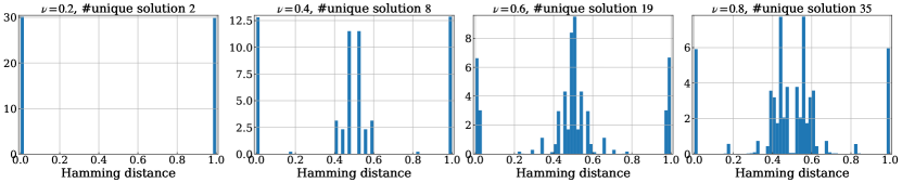
Figure 8: The density of Hamming distance combination of the solution, $\{d_{H}(P_{:s},P_{:l})\}_{1\leq s<l\leq 1000}$ in MaxCut G14, with different parameters $\nu$ and the count of unique solutions

D.2 CTRA for Multi-instance Solutions

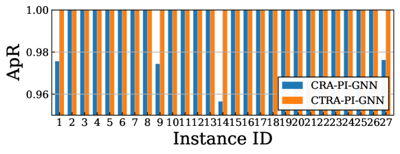
Figure 9: The ApR of DBM (Matching-1) using CTRA-PI-GNN and CRA-PI-solvers (Ichikawa, 2023).

In this section, we numerically demonstrate that the CTRA-PI-GNN solver can efficiently solve multiple problems with similar structures. The numerical experiments solve all $27$ DBM instances using the CTRA-PI-GNN solver with the following loss function:

$$\hat{R}({\bm{\theta}};{\mathcal{C}}_{S},{\bm{\lambda}},\gamma)=\sum_{s=1}^{S}\hat{l}({\bm{\theta}};C_{s},{\bm{\lambda}}_{s})+\Phi({\bm{\theta}};{\mathcal{C}}_{S},\gamma,\alpha),~{}~{}\Phi({\bm{\theta}},{\mathcal{C}}_{S},\gamma,\alpha)\mathrel{\ensurestackMath{\stackon[1pt]{=}{\scriptstyle\Delta}}}\gamma\sum_{i=1}^{N}\sum_{s=1}^{S}(1-(2P_{{\bm{\theta}},is}(C_{s})-1)^{\alpha}).$$

where ${\mathcal{C}}_{S}=\{C_{s},M_{s}\}_{s=1}^{27}$ represents the instance parameters, and $\hat{l}$ is defined as follows:

$$l({\bm{x}};C,M,{\bm{\lambda}})=-\sum_{i,j}C_{ij}x_{ij}+\lambda_{1}\sum_{i}\mathrm{ReLU}\Big{(}\sum_{j}x_{ij}-1\Big{)}+\lambda_{2}\sum_{j}\mathrm{ReLU}\Big{(}\sum_{i}x_{ij}-1\Big{)}\\ +\lambda_{3}\mathrm{ReLU}\Big{(}p\sum_{ij}x_{ij}-\sum_{ij}M_{ij}x_{ij}\Big{)}+\lambda_{4}\mathrm{ReLU}\Big{(}q\sum_{ij}x_{ij}-\sum_{ij}(1-M_{ij})x_{ij}\Big{)},$$

where ${\bm{\lambda}}$ is fixed as ${\bm{\lambda}}=(\lambda_{1},\lambda_{2},\lambda_{3},\lambda_{4})=(2,2,12,12)$. The parameters for the CTRA-PI-GNN solver is set the same as in Section 4.1. On the other hand, the CRA-PI-GNN solver repeatedly solve the $27$ problems using the same settings as Ichikawa (2023). As a result, the CTRA-PI-GNN solver can explore global optimal solutions for all problems. Figure 9 showcases the solutions yielded by both the CRA-PI-GNN and CTRA-PI-GNN solvers for the 27 Matching-1 instances. Matching-2 is excluded from this comparison, given that both solvers achieved global solutions for these instances. The CRA-PI-GNN solver, applied 27 times for Matching-1, accumulated a total runtime of $36{,}925\pm 445$ seconds, significantly longer than the CTRA-PI-GNN’s efficient $5{,}617\pm 20$ seconds. For Matching-2, the CRA-PI-GNN solver required $36{,}816\pm 149$ seconds, whereas the CTRA-PI-GNN solver completed its tasks in just $2{,}907\pm 19$ seconds. The reported errors correspond to the standard deviation from five random seeds. These findings not only highlight the CTRA-PI-GNN solver’s superior efficiency in solving a multitude of problems but also its ability to achieve higher Acceptance Probability Ratios (ApR) compared to the CRA-PI-GNN solver. The consistency of these advantages across different problem types warrants further investigation.

D.3 Additional Results of penalty-diversified solutions for DBM problems

This section extends our discussion on penalty-diversified solutions for DBM problems, as introduced in Section 4.2. In these numerical experiments, we used the same $\Lambda_{S}$ as in Section 4.2 and executed the CTRA-PI-GNN under the same settings as in Section 4.1. As shown in Figure 10, the CTRA-PI-GNN can acquire penalty-diversified solutions for all instances of the DBM.

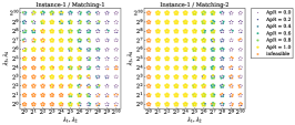
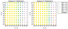
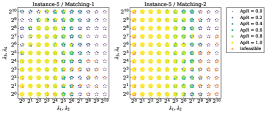
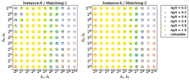
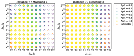
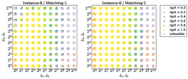
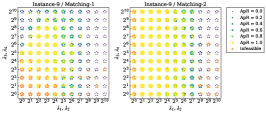
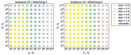
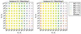
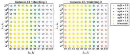
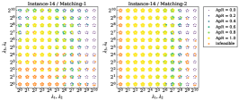
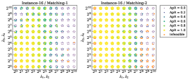
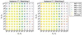
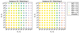
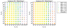
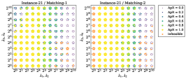
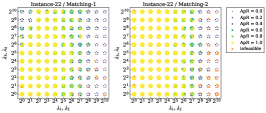
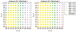
Figure 10: ApR of the DBM problems on th grid $\Lambda_{S}$ using CTRA-PI-GNN solver. Each point on the coordinate plane represents the results from five different random seed, with the colors indicating the ApR. The constraints violation are marked with a cross symbol.

References

- Albash & Lidar (2018) Albash, T. and Lidar, D. A. Adiabatic quantum computation. Reviews of Modern Physics, 90(1):015002, 2018.
- Alidaee et al. (1994) Alidaee, B., Kochenberger, G. A., and Ahmadian, A. 0-1 quadratic programming approach for optimum solutions of two scheduling problems. International Journal of Systems Science, 25(2):401–408, 1994.
- Amizadeh et al. (2018) Amizadeh, S., Matusevych, S., and Weimer, M. Learning to solve circuit-sat: An unsupervised differentiable approach. In International Conference on Learning Representations, 2018.
- Angelini & Ricci-Tersenghi (2023) Angelini, M. C. and Ricci-Tersenghi, F. Modern graph neural networks do worse than classical greedy algorithms in solving combinatorial optimization problems like maximum independent set. Nature Machine Intelligence, 5(1):29–31, 2023.
- Anthony et al. (2017) Anthony, M., Boros, E., Crama, Y., and Gruber, A. Quadratic reformulations of nonlinear binary optimization problems. Mathematical Programming, 162:115–144, 2017.
- Aramon et al. (2019) Aramon, M., Rosenberg, G., Valiante, E., Miyazawa, T., Tamura, H., and Katzgraber, H. G. Physics-inspired optimization for quadratic unconstrained problems using a digital annealer. Frontiers in Physics, 7:48, 2019.
- Barbier et al. (2013) Barbier, J., Krzakala, F., Zdeborová, L., and Zhang, P. The hard-core model on random graphs revisited. In Journal of Physics: Conference Series, volume 473, pp. 012021. IOP Publishing, 2013.
- Baste et al. (2019) Baste, J., Jaffke, L., Masařík, T., Philip, G., and Rote, G. Fpt algorithms for diverse collections of hitting sets. Algorithms, 12(12):254, 2019.
- Baste et al. (2022) Baste, J., Fellows, M. R., Jaffke, L., Masařík, T., de Oliveira Oliveira, M., Philip, G., and Rosamond, F. A. Diversity of solutions: An exploration through the lens of fixed-parameter tractability theory. Artificial Intelligence, 303:103644, 2022.
- Bayati et al. (2010) Bayati, M., Gamarnik, D., and Tetali, P. Combinatorial approach to the interpolation method and scaling limits in sparse random graphs. In Proceedings of the forty-second ACM symposium on Theory of computing, pp. 105–114, 2010.
- Boginski et al. (2005) Boginski, V., Butenko, S., and Pardalos, P. M. Statistical analysis of financial networks. Computational statistics & data analysis, 48(2):431–443, 2005.
- Cappart et al. (2023) Cappart, Q., Chételat, D., Khalil, E. B., Lodi, A., Morris, C., and Velickovic, P. Combinatorial optimization and reasoning with graph neural networks. J. Mach. Learn. Res., 24:130–1, 2023.
- Coello (2002) Coello, C. A. C. Theoretical and numerical constraint-handling techniques used with evolutionary algorithms: a survey of the state of the art. Computer methods in applied mechanics and engineering, 191(11-12):1245–1287, 2002.
- Coja-Oghlan & Efthymiou (2015) Coja-Oghlan, A. and Efthymiou, C. On independent sets in random graphs. Random Structures & Algorithms, 47(3):436–486, 2015.
- Danna & Woodruff (2009) Danna, E. and Woodruff, D. L. How to select a small set of diverse solutions to mixed integer programming problems. Operations Research Letters, 37(4):255–260, 2009.
- Danna et al. (2007) Danna, E., Fenelon, M., Gu, Z., and Wunderling, R. Generating multiple solutions for mixed integer programming problems. In International Conference on Integer Programming and Combinatorial Optimization, pp. 280–294. Springer, 2007.
- Deza & Laurent (1994) Deza, M. and Laurent, M. Applications of cut polyhedra—ii. Journal of Computational and Applied Mathematics, 55(2):217–247, 1994.
- Drosou & Pitoura (2010) Drosou, M. and Pitoura, E. Search result diversification. ACM SIGMOD Record, 39(1):41–47, 2010.
- Ferber et al. (2020) Ferber, A., Wilder, B., Dilkina, B., and Tambe, M. Mipaal: Mixed integer program as a layer. In Proceedings of the AAAI Conference on Artificial Intelligence, volume 34, pp. 1504–1511, 2020.
- Fernau et al. (2019) Fernau, H., Golovach, P., Sagot, M.-F., et al. Algorithmic enumeration: Output-sensitive, input-sensitive, parameterized, approximative (dagstuhl seminar 18421). In Dagstuhl Reports, volume 8. Schloss Dagstuhl-Leibniz-Zentrum fuer Informatik, 2019.
- Fomin et al. (2020) Fomin, F. V., Golovach, P. A., Jaffke, L., Philip, G., and Sagunov, D. Diverse pairs of matchings. arXiv preprint arXiv:2009.04567, 2020.
- Fomin et al. (2023) Fomin, F. V., Golovach, P. A., Panolan, F., Philip, G., and Saurabh, S. Diverse collections in matroids and graphs. Mathematical Programming, pp. 1–33, 2023.
- Gilmer et al. (2017) Gilmer, J., Schoenholz, S. S., Riley, P. F., Vinyals, O., and Dahl, G. E. Neural message passing for quantum chemistry. In International conference on machine learning, pp. 1263–1272. PMLR, 2017.
- Glover et al. (2019) Glover, F., Kochenberger, G., and Du, Y. Quantum bridge analytics i: a tutorial on formulating and using qubo models. 4or, 17:335–371, 2019.
- Hale (1980) Hale, W. K. Frequency assignment: Theory and applications. Proceedings of the IEEE, 68(12):1497–1514, 1980.
- Hamilton et al. (2017) Hamilton, W., Ying, Z., and Leskovec, J. Inductive representation learning on large graphs. Advances in neural information processing systems, 30, 2017.
- Hanaka et al. (2021) Hanaka, T., Kobayashi, Y., Kurita, K., and Otachi, Y. Finding diverse trees, paths, and more. In Proceedings of the AAAI Conference on Artificial Intelligence, volume 35, pp. 3778–3786, 2021.
- Hanaka et al. (2023) Hanaka, T., Kiyomi, M., Kobayashi, Y., Kobayashi, Y., Kurita, K., and Otachi, Y. A framework to design approximation algorithms for finding diverse solutions in combinatorial problems. In Proceedings of the AAAI Conference on Artificial Intelligence, volume 37, pp. 3968–3976, 2023.
- Hebrard et al. (2005) Hebrard, E., Hnich, B., O’Sullivan, B., and Walsh, T. Finding diverse and similar solutions in constraint programming. In AAAI, volume 5, pp. 372–377, 2005.
- Hudson et al. (2021) Hudson, B., Li, Q., Malencia, M., and Prorok, A. Graph neural network guided local search for the traveling salesperson problem. arXiv preprint arXiv:2110.05291, 2021.
- Ichikawa (2023) Ichikawa, Y. Controlling continuous relaxation for combinatorial optimization. arXiv preprint arXiv:2309.16965, 2023.
- Karalias & Loukas (2020) Karalias, N. and Loukas, A. Erdos goes neural: an unsupervised learning framework for combinatorial optimization on graphs. Advances in Neural Information Processing Systems, 33:6659–6672, 2020.
- Karp (2010) Karp, R. M. Reducibility among combinatorial problems. Springer, 2010.
- Kingma & Ba (2014) Kingma, D. P. and Ba, J. Adam: A method for stochastic optimization. arXiv preprint arXiv:1412.6980, 2014.
- Kochenberger et al. (2014) Kochenberger, G., Hao, J.-K., Glover, F., Lewis, M., Lü, Z., Wang, H., and Wang, Y. The unconstrained binary quadratic programming problem: a survey. Journal of combinatorial optimization, 28:58–81, 2014.
- Korte et al. (2011) Korte, B. H., Vygen, J., Korte, B., and Vygen, J. Combinatorial optimization, volume 1. Springer, 2011.
- Lamb et al. (2020) Lamb, L. C., Garcez, A., Gori, M., Prates, M., Avelar, P., and Vardi, M. Graph neural networks meet neural-symbolic computing: A survey and perspective. arXiv preprint arXiv:2003.00330, 2020.
- Mandi et al. (2022) Mandi, J., Bucarey, V., Tchomba, M. M. K., and Guns, T. Decision-focused learning: through the lens of learning to rank. In International Conference on Machine Learning, pp. 14935–14947. PMLR, 2022.
- Mulamba et al. (2020) Mulamba, M., Mandi, J., Diligenti, M., Lombardi, M., Bucarey, V., and Guns, T. Contrastive losses and solution caching for predict-and-optimize. arXiv preprint arXiv:2011.05354, 2020.
- Neven et al. (2008) Neven, H., Rose, G., and Macready, W. G. Image recognition with an adiabatic quantum computer i. mapping to quadratic unconstrained binary optimization. arXiv preprint arXiv:0804.4457, 2008.
- Papadimitriou & Steiglitz (1998) Papadimitriou, C. H. and Steiglitz, K. Combinatorial optimization: algorithms and complexity. Courier Corporation, 1998.
- Petit & Trapp (2015) Petit, T. and Trapp, A. C. Finding diverse solutions of high quality to constraint optimization problems. In IJCAI. International Joint Conference on Artificial Intelligence, 2015.
- Petit & Trapp (2019) Petit, T. and Trapp, A. C. Enriching solutions to combinatorial problems via solution engineering. INFORMS Journal on Computing, 31(3):429–444, 2019.
- Scarselli et al. (2008) Scarselli, F., Gori, M., Tsoi, A. C., Hagenbuchner, M., and Monfardini, G. The graph neural network model. IEEE transactions on neural networks, 20(1):61–80, 2008.
- Schuetz et al. (2022a) Schuetz, M. J., Brubaker, J. K., and Katzgraber, H. G. Combinatorial optimization with physics-inspired graph neural networks. Nature Machine Intelligence, 4(4):367–377, 2022a.
- Schuetz et al. (2022b) Schuetz, M. J., Brubaker, J. K., Zhu, Z., and Katzgraber, H. G. Graph coloring with physics-inspired graph neural networks. Physical Review Research, 4(4):043131, 2022b.
- Schuetz et al. (2023) Schuetz, M. J., Brubaker, J. K., and Katzgraber, H. G. Reply to: Modern graph neural networks do worse than classical greedy algorithms in solving combinatorial optimization problems like maximum independent set. Nature Machine Intelligence, 5(1):32–34, 2023.
- Sen et al. (2008) Sen, P., Namata, G., Bilgic, M., Getoor, L., Galligher, B., and Eliassi-Rad, T. Collective classification in network data. AI magazine, 29(3):93–93, 2008.
- Smith et al. (1997) Smith, A. E., Coit, D. W., Baeck, T., Fogel, D., and Michalewicz, Z. Penalty functions. Handbook of evolutionary computation, 97(1):C5, 1997.
- Toenshoff et al. (2019) Toenshoff, J., Ritzert, M., Wolf, H., and Grohe, M. Run-csp: unsupervised learning of message passing networks for binary constraint satisfaction problems. CoRR, abs/1909.08387, 2019.
- Van Hentenryck et al. (2009) Van Hentenryck, P., Coffrin, C., and Gutkovich, B. Constraint-based local search for the automatic generation of architectural tests. In Principles and Practice of Constraint Programming-CP 2009: 15th International Conference, CP 2009 Lisbon, Portugal, September 20-24, 2009 Proceedings 15, pp. 787–801. Springer, 2009.
- Vieira et al. (2011) Vieira, M. R., Razente, H. L., Barioni, M. C., Hadjieleftheriou, M., Srivastava, D., Traina, C., and Tsotras, V. J. On query result diversification. In 2011 IEEE 27th International Conference on Data Engineering, pp. 1163–1174. IEEE, 2011.
- Wang & Li (2023) Wang, H. and Li, P. Unsupervised learning for combinatorial optimization needs meta-learning. arXiv preprint arXiv:2301.03116, 2023.
- Wang et al. (2022) Wang, H. P., Wu, N., Yang, H., Hao, C., and Li, P. Unsupervised learning for combinatorial optimization with principled objective relaxation. Advances in Neural Information Processing Systems, 35:31444–31458, 2022.
- Wang et al. (2019) Wang, M., Zheng, D., Ye, Z., Gan, Q., Li, M., Song, X., Zhou, J., Ma, C., Yu, L., Gai, Y., et al. Deep graph library: A graph-centric, highly-performant package for graph neural networks. arXiv preprint arXiv:1909.01315, 2019.
- Ye (2003) Ye, Y. The gset dataset. https://web.stanford.edu/~yyye/yyye/Gset/, 2003.