Evolution Guided Generative Flow Networks

Abstract

Generative Flow Networks (GFlowNets)are a family of probabilistic generative models that learn to sample compositional objects proportional to their rewards. One big challenge of GFlowNets is training them effectively when dealing with long time horizons and sparse rewards. To address this, we propose Evolution guided generative flow networks (EGFN), a simple but powerful augmentation to the GFlowNets training using Evolutionary algorithms (EA). Our method can work on top of any GFlowNets training objective, by training a set of agent parameters using EA, storing the resulting trajectories in the prioritized replay buffer, and training the GFlowNets agent using the stored trajectories. We present a thorough investigation over a wide range of toy and real-world benchmark tasks showing the effectiveness of our method in handling long trajectories and sparse rewards.

1 Introduction

Generative Flow Networks (GFlowNets)(Bengio et al., 2021, 2023) are a family of probabilistic amortized samplers that learns to sample from a space proportionally to some reward function $R(x)$, effectively sampling compositional objects over some probability distribution. As a generative process, it composes objects by some sequence of actions, terminating by reaching a termination state.

GFlowNets have shown great potential for diverse challenging applications, such as molecule discovery (Jain et al., 2023a), biological sequence design (Jain et al., 2022), combinatorial optimization (Zhang et al., 2023a), latent variable sampling (Liu et al., 2023) and road generation (Ikram et al., 2023). The key advantage of GFlowNets over other methods such as reinforcement learning (RL)is that GFlowNets’s key objective is not reward maximization, allowing them to sample diverse samples from different peaks of high rewards. Although entropy-regularized RL also encourages randomness when taking actions, it is not general in when the underlying graph is not a tree (i.e., a state can have multiple parent states) (Zhao et al., 2019).

Despite the recent advancements, the real-world adaptation of GFlowNets is still limited by a major problem: temporal credit assignment for long trajectories and sparse rewards. For example, real-world problems such as protein design often are often long-horizon problems, necessitating long trajectories for sampling. Since reward is given only when the agent reaches the terminal states, associating intermediate actions with rewards over a lengthy trajectory becomes challenging. Additionally, reward space is sparse in real-world tasks, making temporal credit assignment more difficult. Trajectory balance (TB)objective (Malkin et al., 2022) attempts to tackle the problem by matching the flow across the entire trajectory, but in practice, it induces larger variance and is highly sensitive to sparse rewards (Madan et al., 2023), making the training unstable.

Evolutionary algorithms (EA)(Bäck & Schwefel, 1993), a class of optimization algorithms inspired by natural selection and evolution, can be a promising candidate for tackling the said challenges. Indeed, the shortcomings of GFlowNets are the advantages of EA, which makes it promising to consider incorporating EA into the learning paradigm of GFlowNets to leverage the best from both worlds. First, the selection operation in EA is achieved by fitness evaluation throughout the entire trajectory, which makes them robust to long trajectories and sparse rewards as they naturally bias towards regions with high expected returns. Secondly, mutation makes EA naturally exploratory, which is crucial for GFlowNets training and mode-finding as they rely on diverse samples for better training (Pan et al., 2022b). Third, EA’s natural selection biases towards parameters that generate high reward samples, which, coupled with a replay buffer, can provide sample redundancy, resulting in a better gradient signal for stable GFlowNets training.

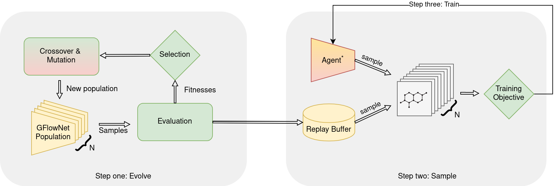
Figure 1: The proposed EGFN architecture. Step one provides high-quality trajectories to the replay buffer. Step two gathers training trajectories from both online and offline trajectories. Step three trains the star agent using the training trajectories.

In this work, we introduce Evolution guided generative flow networks (EGFN), a novel training method for GFlowNets combining gradient-based and gradient-free approaches and benefit from the best of both worlds. Our proposed approach is a three-step training process. First, using a fitness metric across sampled trajectories taken over a population of GFlowNets agents, we perform selection, crossover, and mutation on neural network parameters of GFlowNets agents to generate a new population. To reuse the population’s experience, we store the evaluated trajectories in the prioritized replay buffer (PRB). For the second step, we sample the stored trajectories from a prioritized replay buffer (PRB)and combine them with online samples from a different GFlowNets agent. Finally, using the gathered samples, we train a GFlowNets agent using gradient descent over some objectives such as Flow matching (FM), TB, and Detailed balance (DB). The reward-maximizing capability of EA enhances gradient signal through high reward training samples, ensuring stable GFlowNets training even in conditions with sparse rewards and long trajectories. Through extensive evaluation in experimental and a wide range of real-world settings, our method proves effective in addressing weaknesses related to temporal credit assignment in sparse rewards and long trajectories, surpassing GFlowNets baselines in terms of both the number of re-discovered modes and top-K rewards.

2 Preliminaries

2.1 Generative Flow Networks (GFlowNets)

Generative Flow Networks (GFlowNets) are a family of generative models that samples compositional objects through a sequence of actions. Given a terminal state space $\mathcal{X}$, they aim to learn a stochastic policy $\pi$ that can sample terminal states $x\in\mathcal{X}$ proportionally to a non-negative reward function $R(x)$, i.e., $\pi(x)\propto R(x)$. GFlowNets construct objects $x\in\mathcal{X}$ by sampling constructive, irreversible actions $a\in\mathcal{A}$ that transition $s_{t}$ to $s_{t+1}$. We denote the Markovian composition trajectory $(s_{0}\rightarrow s_{1}\xrightarrow{}\dots\rightarrow x)$ as $\tau\in\mathcal{T}$, where $\mathcal{T}$ is the set of all trajectories. Thus, the problem is formulated as a directed acyclic graph (DAG), $(\mathcal{S},\mathcal{E})$, where each node in $\mathcal{S}$ denotes a state with an initial state $s_{0}$, and each edge in $\mathcal{E}$ denotes a transition $s_{t}\rightarrow s_{t+1}$ with a special terminal action indicating $s=x\in\mathcal{X}$. There exist different paths leading to the same state in the DAG. An important advantage of GFlowNets is that GFN can sample proportionally to different peaks of reward and we can train it in both online and offline settings, allowing us to train from replay buffers.

The key objective of GFlowNets training is to train $P_{F}$ such that $\pi(x)\propto R(x)$, where,

$$\pi(x)=\sum_{\tau\in\mathcal{T}:x\in\tau}\prod_{t=0}^{|\tau-2|}{P_{F}(s_{t+1}|s_{t};\theta)}$$ (1)

where, $P_{F}$ is a parametric model reprenting the forward transition probability of $s_{t}$ to $s_{t+1}$ with parameter $\theta$. There are several widely used loss functions to optimize GFlowNets including FM, DB and TB.

Flow matching Following Bengio et al. (2021), we define the state flow and edge flow functions $F(s)=\sum_{s\in\tau}{F(\tau)}$ and $F(s\rightarrow s^{\prime})=\sum_{\tau=(\dots s\rightarrow s^{\prime}...)}{F(\tau)}$, respectively. Then, the FM criterion matches the in-flow and the out-flow for all states $s\in\mathcal{S}$, formally –

$$\sum_{s:(s\rightarrow s^{\prime})\in\mathcal{A}}{F(s\rightarrow s^{\prime})}=\sum_{s^{\prime\prime}:(s^{\prime}\rightarrow s^{\prime\prime})\in\mathcal{A}}{F(s^{\prime}\rightarrow s^{\prime\prime})}$$ (2)

where $F(s^{\prime}\rightarrow s^{\prime\prime})=R(s)$ if $s\in\mathcal{X}$. Using $P_{F}(s^{\prime}|s,\theta)=F(s^{\prime}\rightarrow s^{\prime\prime})$, we turn equation 2 to a loss function –

$$\mathcal{L}_{\text{FM}}(s^{\prime},\theta)=\left[\text{log}\frac{\sum_{(s\rightarrow s^{\prime})\in\mathcal{A}}{P_{F}(s^{\prime}|s,\theta)}}{\sum_{(s^{\prime}\rightarrow s^{\prime\prime})\in\mathcal{A}}{P_{F}(s^{\prime}|s^{\prime\prime},\theta)}}\right]^{2}$$ (3)

Detailed balance Following Bengio et al. (2023), we parameterize $F(s)$, $F(s\rightarrow s^{\prime})$, and $F(s^{\prime}\rightarrow s)$ with $F_{\theta}(s)$, $P_{F}(s^{\prime}|s,\theta)$, and $P_{B}(s|s^{\prime},\theta)$, respectively. Then, the DB loss for a sampled trajectory $\tau\in\mathcal{T}$ is –

$$\mathcal{L}_{\text{DB}}(s,s^{\prime},\theta)=\left[\text{log}\frac{F_{\theta}(s)P_{F}(s^{\prime}|s,\theta)}{F_{\theta}(s^{\prime})P_{B}(s|s^{\prime},\theta)}\right]^{2}$$ (4)

for all $(s\rightarrow s^{\prime})\in\tau$.

Trajectory balance Malkin et al. (2022) extends the detail balance objective to the trajectory level, via a telescoping operation of Eq. (4). Specifically, $Z_{\theta}$ is a learnable parameter that represents the total flow: $\sum_{x\in\mathcal{X}}{R(x)}=\sum_{s:s_{0}\rightarrow s\in\tau\forall\tau\in\mathcal{T}}{P_{F}(s|s_{0};\theta)}$, and the TB loss is defined as:

$$\mathcal{L}_{\text{TB}}(\tau,\theta)=\left[\text{log}\frac{Z_{\theta}\prod_{t=0}^{|\tau|-1}{P_{F}(s_{t+1}|s_{t},\theta)}}{R(x)\prod_{t=0}^{|\tau|-1}{P_{B}(s_{t}|s_{t+1},\theta)}}\right]^{2}.$$ (5)

This can incur larger variance as demonstrated in Madan et al. (2023).

We train the GFlowNets parameter $\theta$ by minimizing the loss $\mathcal{L}$ by performing stochastic gradient descent.

Algorithm 1 Evolution Guided GFlowNet Training

Input:
$P_{F}^{*}$: Forward flow of the star agent with weights $\theta^{*}$
$pop_{F}$: Population of k agents with randomly initiated weights
$\mathcal{D}$ : Prioritized replay buffer
$\mathcal{E}$: Number of episodes in an evaluation
$\epsilon$: percent of greedily selected elites
$\delta$: online-to-offline sample ratio
$\gamma$: mutation strength
for each episodes do

       for each $P_{F}\in pop_{F}$ do

             fitness, $\mathcal{D}$ = EVALUATE($P_{F}$, $\mathcal{E}$, noise = None, $\mathcal{D}$);

              // store experience in replay buffer

      Sort $pop_{F}$ based on fitness in a descending order
Select the first $\epsilon$k $P_{F}$ from $pop_{F}$ as $elite$
Select (1 - $\epsilon$) $P_{F}$ from $pop_{F}$ stochastically based on fitness as $S$
while $|S|<$ k do

             crossover between $P_{F}\in elite$ and $P_{F}\in S$ and append to $S$

      for each $P_{F}\in S$ do

             Apply mutation $\sim\mathcal{N}(0,\gamma)$ to $\theta_{P_{F}}$ with probability $p_{mutation}$

      fitness, $\mathcal{D}$ = EVALUATE($P_{F}^{*}$, $\mathcal{E}$, $\mathcal{D}$)
Sample a minibatch of $(1-\delta)T$ offline trajectories $\mathcal{T}$ from $\mathcal{D}$
Sample a minibatch of $\delta T$ online trajectories $\mathcal{T}$ from $P_{F}^{*}$
Compute loss $\mathcal{L}$ using trajectory balance loss from $\mathcal{T}$
Update parameters $\theta^{*}$ using stochastic descent on loss $\mathcal{L}$

2.2 Evolutionary algorithms (EA)

Evolutionary algorithms (EA)(Bäck, 2006; Spears et al., 1993) are a class of combinatorial optimization algorithms that generally rely on three key techniques: mutation, crossover, and selection as in biological evolution. The crossover operation is responsible for generating new samples based on exchange of segments among a population of samples. The mutation operation alters the generated samples, usually with some probability $p_{mutation}$. Finally, the selection operation evaluates the fitness score of the population and is responsible for generating the next population. In this work, we apply EA in the context of the weights of the neural networks, often referred to as neuroevolution (Stanley & Miikkulainen, 2002b; Risi & Togelius, 2014; Floreano et al., 2008; Lüders et al., 2017).

3 Evolution guided generative flow networks (EGFN)

EGFN is an augmentation of existing training methods of GFlowNets. The evolutionary part in EGFN (Step one) samples discrete objects, e.g., a molecular structure, using a population of GFlowNets agents, evaluates the fitness of the agents based on the samples, and generates better samples by manipulating the weights of the agent population. We store the samples obtained from the population in a PRB that the GFlowNets sampler uses to, alongside on-policy samples, train its weights (Step two & three). To differentiate the GFlowNets agent trained by gradient descent in step two and three from the agent population trained by EA in step one, we refer to the agent trained by gradient descent as the star agent and GFlowNets agents trained by EA as EA GFlowNets agents. The training loop can be summarized in the following three steps:

Step One

Generate a population of EA GFlowNets agents. Evaluate the fitness of the agents’ weights by evaluating the samples gathered from the agents’. Apply the necessary selection, mutation, and crossover to the weights to generate the next population. Store the generated trajectories $\{(\tau_{1},\dots,\tau_{\mathcal{E}})_{1},\tau_{1},\dots,\tau_{\mathcal{E}})_{2},\dots,(\tau_{1},\dots,\tau_{\mathcal{E}})_{k}\}$ to the PRB.

Step Two

Gather online trajectories from star agent $P_{F}^{*}$ and offline samples from PRB.

Step Three

Train $P_{F}^{*}$ using $\{\tau_{1},\tau_{2},\dots,\tau_{T}\}$ using gradient descent on any GFlowNets loss function such as equations 3, 4, or 5.

3.1 Step one: Evolve

This step involves optimizing EA GFlowNets agent weights to produce trajectories that accelerate $P_{F}^{*}$ training using the PRB. To this end, before the train begins, we initialize $pop$, a population of $k$ EA GFlowNets agents with random weights. We optimize the population weights in a standard EA process that contains selection, crossover, and mutation. Algorithm 2 in the appendix C details the evaluation process.

Selection The selection process begins with an evaluation of the population by calculating each agent’s fitness scores. We define the fitness score of an agent by the mean reward of $\mathcal{E}$ trajectories $\{\tau_{1},\tau_{2},\dots,\tau_{\mathcal{E}}\}$ sampled from the agent. Next, based on fitness scores, we transfer the top $\epsilon$% $elite$ agents’ weights to the next population, unmodified. Notably, we store the $k\mathcal{E}$ trajectories sampled from this step to the PRB in this step.

Crossover The crossover step ensures weight mixing between agents’, ensuring stochasticity. Here, we perform the crossover in two steps. First, we perform a selection tournament process among the agents to get $pop$ - $elite$ agents, sampling proportionally to their fitness value and performing crossover among them. Next, we perform a crossover between the unselected agents and $elite$. We combine the two sets of agents and pass them on to the mutation process.

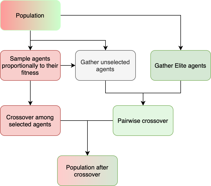
Figure 2: The crossover operation in EGFN. Here, we fill a proportion of population through the crossover between agents selected proportionally to their fitness. We fill the rest with the crossover between the unselected agents and the elite agents.

Mutation The mutation process ensures natural exploration among agents. We apply mutation by adding a gaussian perturbation $\mathcal{N}(0,\gamma)$ to the agent weights. In this work, we only apply mutation to the non-$elite$ agents.

3.2 Step two: Sample

In this step, we gather trajectory samples $\{\tau_{1},\tau_{2},\dots,\tau_{T}\}$ to train the star agent. We use both online trajectories sampled by the star agent and offline trajectories stored in the PRB. For online trajectories, we construct a trajectory $\tau$ by applying $P_{F}^{*}$ to get $s_{0}\rightarrow s_{1}\rightarrow\dots\rightarrow x,x\in\mathcal{X}$, where $\mathcal{X}$ is the set of all terminal states. It is noteworthy that there are many works (Rector-Brooks et al., 2023; Kim et al., 2023; Pan et al., 2023a, 2022a) that augment or perturb the online trajectories by applying stochastic exploration, temperature scaling, etc. In this work, we choose a simple on-policy sampling from $P_{F}^{*}$ to get the online trajectories. For offline samples, we simply use PRB to sample trajectories collected from step one proportionally to the terminal reward. For this work, we take a simple approach for PRB, uniformly sampling 50% trajectories from the 20 percentile and 50% trajectories from the rest.

3.3 Step three: Train

We train the star agent by calculating loss $\mathcal{L}$ using equation 3, 4, or 5 and minimizing the loss by applying stochastic gradient descent to the parameter $\theta$.

4 Experiments

In this section, we validate EGFN for different synthetic and real-world tasks. 4.1 presents an investigation of EGFN’s performance in long trajectory and sparse rewards, generalizability across multiple GFlowNets objectives, and an ablation study on different components. Next, we present three real-world molecule generation experiments in 4.2, 4.3, and 4.4. Finally, we present an experiment summary. For all the following experiments, we use $k=10$, $\mathcal{E}=4$, $\epsilon=0.2$, and $\gamma=1$. For fair comparison, we equip all baselines with a replay buffer of comparable settings to the EGFN. All result figures report the mean and variance over three random seeds.

4.1 Synthetic tasks

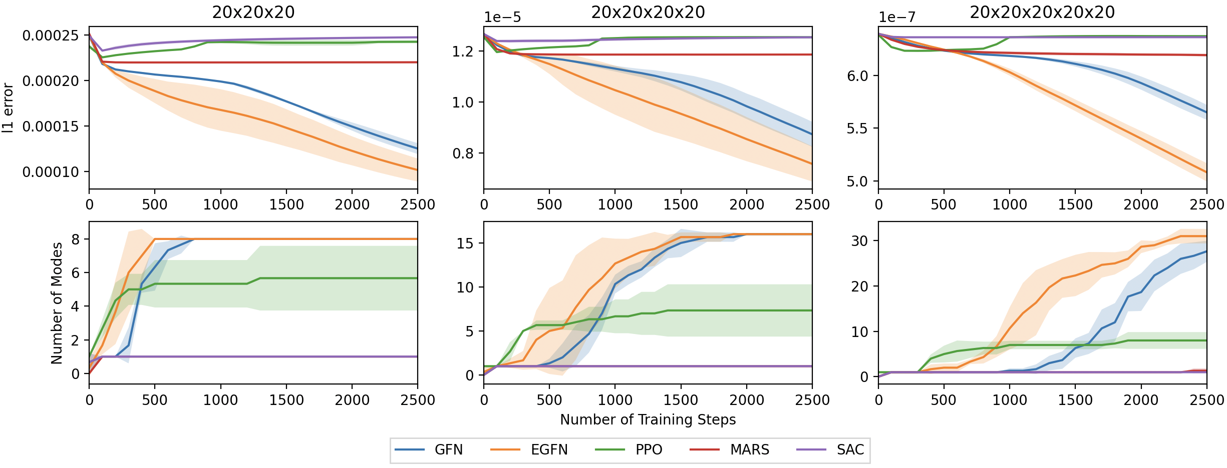
Figure 3: Left: An example hypergrid environment for $\text{dimension }D=2,\text{horizon }H=16$. Here, the $2^{2}=4$ yellow tiles refer to the high reward modes. Right: Experimental results comparison for the hypergrid task between EGFN, GFlowNets, RL, and MCMC baseline across increasing dimensions for 2500 training steps. Right top: the $\ell_{1}$ error between the learned distribution density and the true target density. Right bottom: the number of discovered modes across the training process. As the dimension of the grid increases, the trajectory length also increases. The proposed EGFN method achieves better performance than all baselines, with broader performance gap between EGFN and GFlowNets with increasing trajectory length.

We first study the effectiveness of EGFN investigating the well-studied hypergrid task introduced by Bengio et al. (2021). The hypergrid is a $D$-dimensional environment of $H$ horizons, with a $H^{D}$ state-space, $D+1$ action-space, and $2^{D}$ modes. The $i$th action in the action space corresponds to moving 1 step in the $i$th dimension, with the $D$th action being a termination action with which the agent completes the trajectory and gets a reward specified by equation 6.

In this empirical experiment, two questions interest us.

• Does EGFN augmentation provide improvement against the best GFlowNets baseline for longer trajectories and sparse rewards?

• Is this method generally applicable to other baselines?

Setup We run all hypergrid experiments for $D\in\{3,4,5\}$, $H=20$, and $R_{0}\in\{10^{-3},10^{-4},10^{-5}\}$. To determine the best GFlowNets baseline, we run three objectives $\in\{\text{\lx@glossaries@gls@link{acronym}{fm}{\leavevmode FM}},\text{\lx@glossaries@gls@link{acronym}{tb}{\leavevmode TB}},\text{\lx@glossaries@gls@link{acronym}{db}{\leavevmode DB}}\}$ (please see figure 7 below) and decide to use DB with a PRB of size 1000. For a fair comparison, we use DB for implementing EGFN. We use $R_{0}=10^{-5}$ for the long trajectory experiment and $D=5$ for the reward sparsity experiment, keeping other variables fixed. Finally, we present an ablation study on different components used in our experiments for $H=16,D=5,\text{and }R_{0}=10^{-5}$.

For a complete picture, we compare our method with RL baselines such as PPO (Schulman et al., 2017) and SAC (Haarnoja et al., 2018; Christodoulou, 2019) and MCMC baseline such as MARS (Xie et al., 2020).

Long time horizon result In this experiment, as $D$ increases, $|\tau|$ increases, showing the performance over increasing $|\tau|$. Figure 3 demonstrates that EGFN outperforms GFlowNets baseline both in terms of mode finding efficiency and L1 error. Notably, as $|\tau|$ increases, the performance gap increases, confirming its efficacy in challenging environments. Unexpectedly, MARS prove to be very slow for these challenging environments. Besides, while RL baseline such PPO competes with GFlowNets and EGFN in the beginning, it fails to discover all modes due to its mode maximization objective.

Figure 4: Experimental results for the hypergrid task on different components of EGFN. Top: the $\ell_{1}$ error between the learned distribution density and the true target density. Bottom: the number of discovered modes across the training process. Here, $H=20,D=5$, and we use DB objective. We observe that PRB itself does not improve the results, but when it is coupled with mutation, the results improve.

Reward sparsity result Next, to understand the effect of sparse rewards, we compare our method against GFlowNets. With a decreasing $R_{0}$, reward sparsity increases. Figure 5 shows that EGFN outperforms traditional GFlowNets. Similar to the previous experiment, we see an increasing performance gap as the reward sparsity increases. Similar to previous experiment, both RL and MCMC baselines are no match for such difficult environments.

Different training objectives To see how well EGFN works with different GFlowNets objectives, we show the result of augmentation of our method over all three GFlowNets objectives in figure 7. We see that EGFN offers a steady improvement across all three GFlowNets objectives.

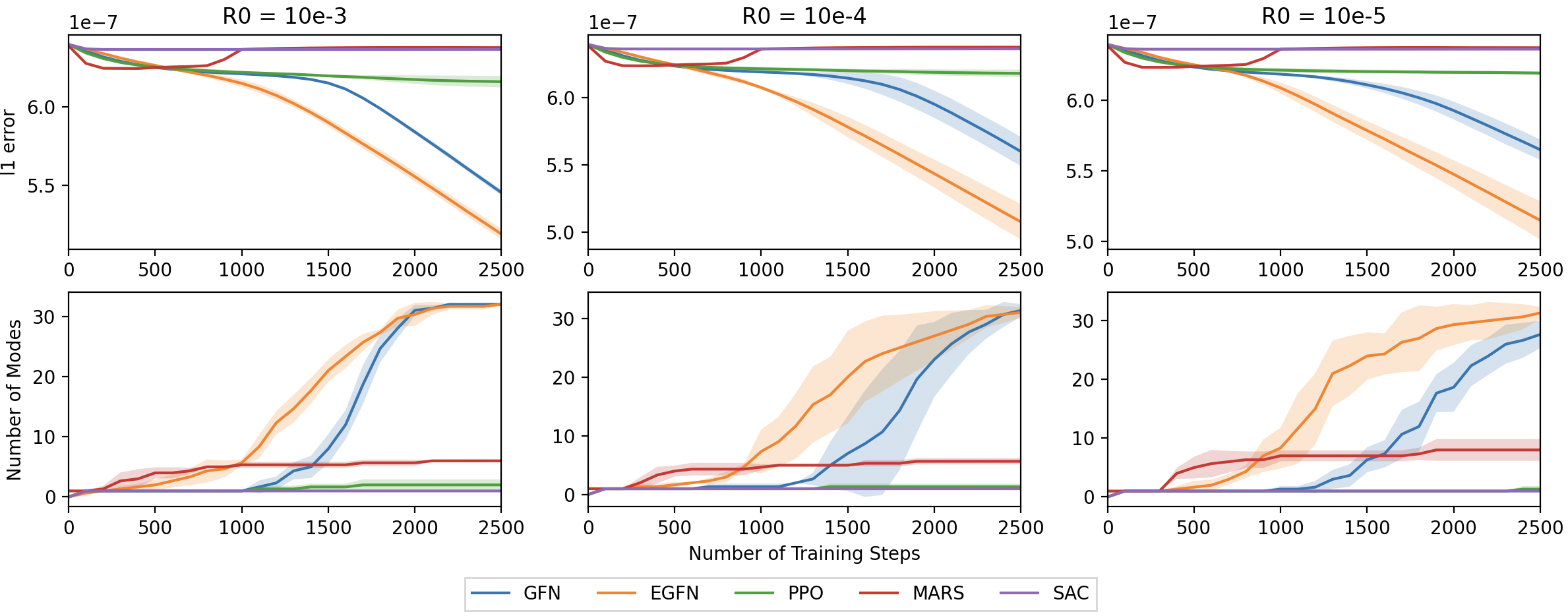
Figure 5: Experimental results comparison for the hypergrid task between EGFN, GFlowNets, RL, and MCMC baseline across increasing dimensions for 2500 training steps. Top: the $\ell_{1}$ error between the learned distribution density and the true target density. Bottom: the number of discovered modes across the training process. Here, $H=20,D=5$. As the $R_{0}$ value decreases, the reward sparsity increases. The proposed EGFN method achieves better performance than all baselines, with broader performance gap between EGFN and GFlowNets with increasing sparsity.

Ablation study result To understand the individual effect of each component of our method, we run the hypergrid experiment by comparing our method against the same without PRB and mutation. Figure 4 details the results of the experiment, underscoring the importance of the mutation operator in EGFN. It shows that PRB individually is not effective for improved results, but when it is coupled with mutation, our method delivers better results.

4.2 Soluable Epoxy Hydrolase (sEH)binder generation task $\left(|\mathcal{X}|\approx 10^{16}\right)$

Setup In this experiment, we are interested in generating molecules with desired chemical properties that are not too similar to one another. Here, we represent molecules states as graph structures and actions as a vocabulary of blocks specified by junction tree modeling (Bickerton et al., 2012; Shi et al., 2020). In the pharmaceutical industry, drug-likeliness (Bickerton et al., 2012), synthesizability (Shi et al., 2020), and toxicity are crucial properties. Hence, we are interested in finding diverse candidate molecules for a given criteria to increase chances for post-selection. Here, the criteria is the molecule’s binding energy to the 4JNC inhibitor of the soluble epoxide hydrolase (sEH) protein. To this end, we train a proxy reward function for predicting the negative binding energy that serves as the reward function. We perform the experiment following the experimental details and reward function specifications from Bengio et al. (2021); Zhang et al. (2023b). Since we are interested in both the diversity and efficacy of drugs, we define a mode as a molecule with a reward greater than 7.5 and a Tanimoto similarity among previous modes less than 0.7. We use FM as the GFlowNets baseline and implement EGFN for the same objective.

Results Since the state space is large, we show the result of the number of modes with reward threshold of 7.5 and 8.0, the top-100, and the top-1000 over the first $2.5\times 10^{4}$ states visited. Figure 10 confirms that EGFN outperforms GFlowNets baseline for mode discovery. Remarkably, EGFN discovers rare molecules with very high reward ($R>8$) that GFlowNets fails to discover. Besides, EGFN has a better top-100 and top-1000 reward performance than GFlowNets baseline, soliciting its mode diversity, which is essential in a molecular discovery setting.

4.3 Transcription factor binder generation task $\left(|\mathcal{X}|\approx 70000\right)$

Setup In this experiment, we generate a nucleotide sequence as a string of length 8. Although the string could be generated autoregressively, in this experiment setting, we use a Prepend-Append Markov decision process (PA-MDP), used in similar settings by Shen et al. (2023); Ikram et al. (2023). Using this MDP, GFlowNets agent actions prepend or append to the nucleotide string. The reward is a DNA binding affinity to a human transcription factor provided by Trabucco et al. (2022). We attempt three GFlowNets objectives, finally deciding to use TB as the best GFlowNets baseline and implement EGFN with the same using a reward exponent $\beta=3$.

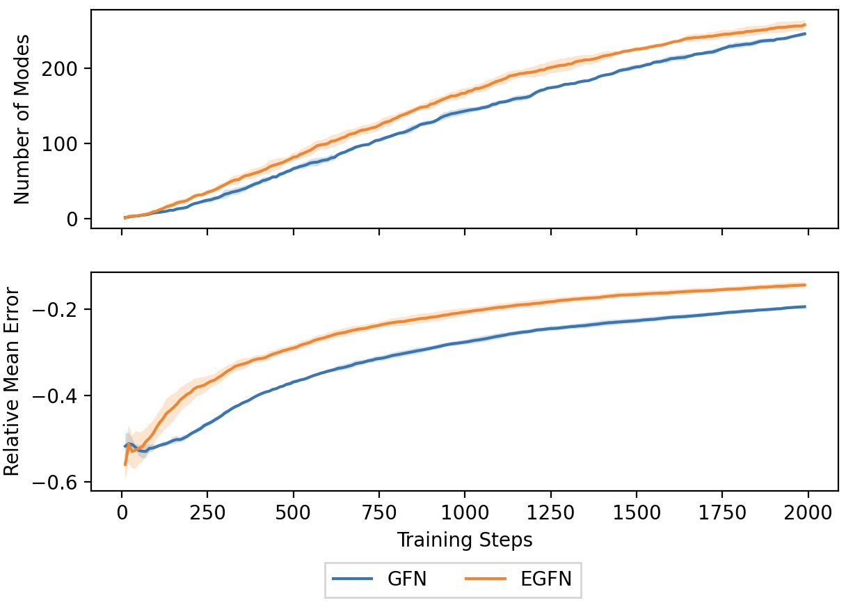
Figure 6: Experiment results for transcription factor binder generation task over 2000 training steps for $\beta=3$. Top: the number of discovered modes across the training process. Bottom: the relative mean error. The proposed augmentation with EGFN achieves better results. GFlowNets implementation uses TB objective.

Results Figure 6 shows the result over 2000 training steps, showing that GFlowNets outperforms GFlowNets baseline both in terms of the number of modes discovered and the mean relative error.

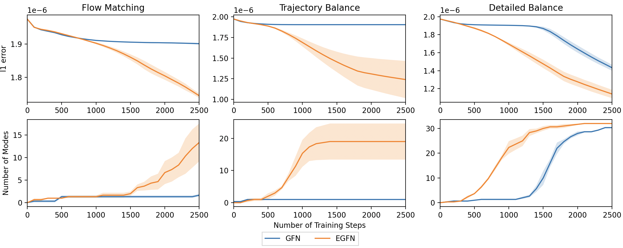
Figure 7: Experimental results for the hypergrid task between EGFN and GFN across different GFlowNets objectives. Top: the $\ell_{1}$ error between the learned distribution density and the true target density. Bottom: the number of discovered modes across the training process. The proposed augmentation with EGFN achieves better results for all three objectives.

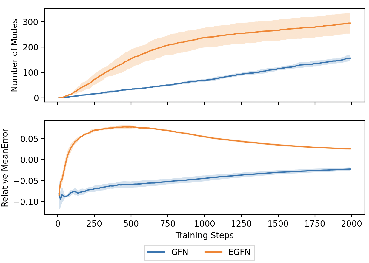
Figure 8: From top to bottom: Example molecule produced in the qm9 task with SMILES representation C1CCCCC1NOCFO. Experiment results for small molecule generation task on the QM9 data over 2000 training steps for $\beta=1$. The number of discovered modes across the training process. The relative mean error. The proposed augmentation with EGFN achieves better results. GFlowNets implementation uses TB objective.

4.4 Small molecule generation Task $\left(|\mathcal{X}|\approx 60000\right)$

Setup In this experiment, we generate a small molecule graph based on the QM9 data (Ramakrishnan et al., 2014) that maximizes the energy gap between its HOMO and LUMO orbitals, thereby increasing its stability. The resulting molecule is a 5-block molecule, having a choice among 12 blocks for its two stems. For the reward function, we use a pre-trained MXMNet proxy by Zhang et al. (2020) with a reward exponent $\beta=1$. Similar to 4.3, we use TB for this experiment.

Results In figure 8, we report the mode discovery and L1 error results over 2000 training steps. Similar to previous experiments, EGFN maintains a steady improvement over the GFlowNets baseline for mode discovery while decreasing the L1 error quicker.

4.5 Result summary

In both the synthetic and real-world experiments, EGFN performs well for mode discovery using fewer training steps than GFlowNets baseline. The performance gap increases with increasing trajectory length and reward sparsity. We also discover that the mutation operator is the most important factor for performance improvement.

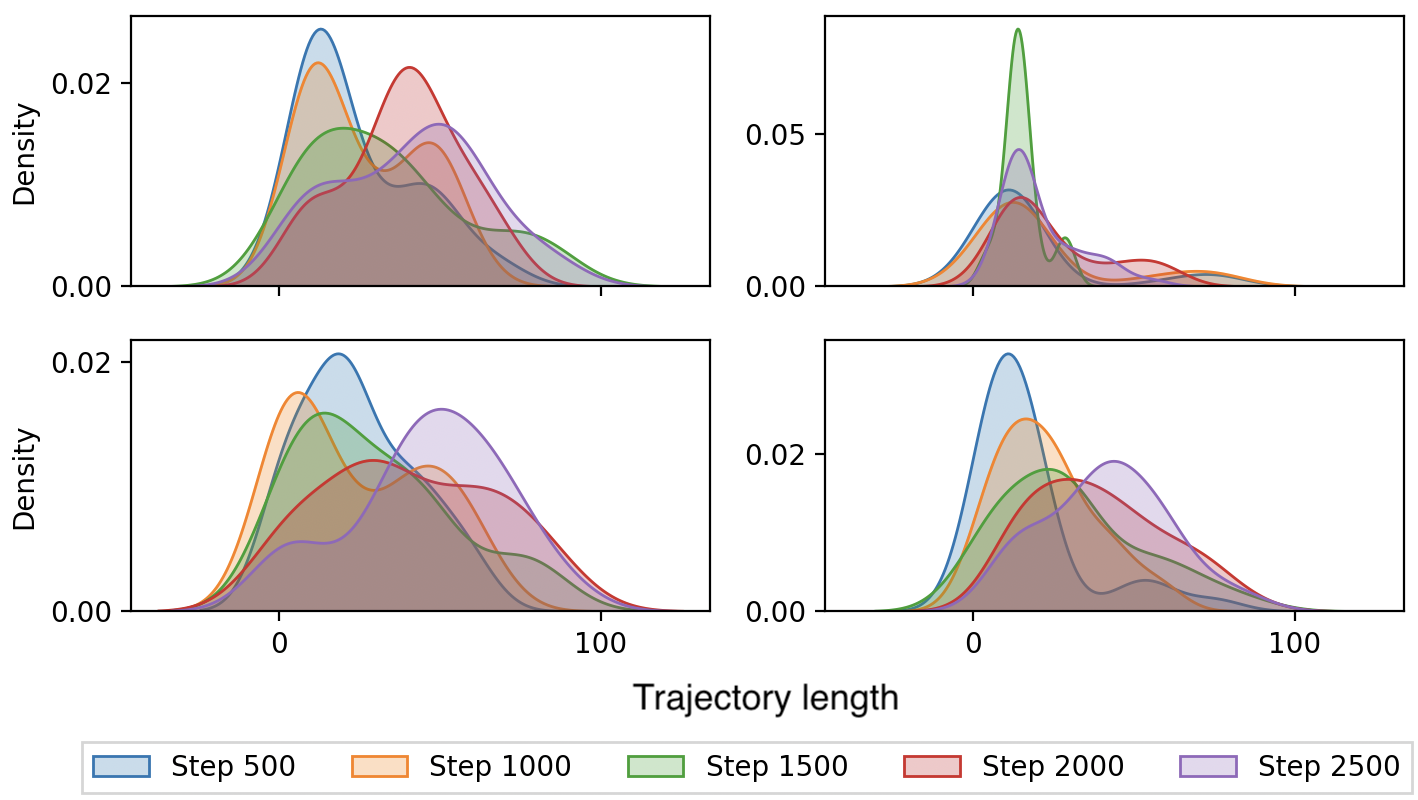
Figure 9: Experimental results for the trajectory lengths of the trajectories stored in the training samples across different training steps for $R_{0}=10^{-2}$ (left) and $10^{-4}$ (right). Top: GFlowNets Bottom: EGFN

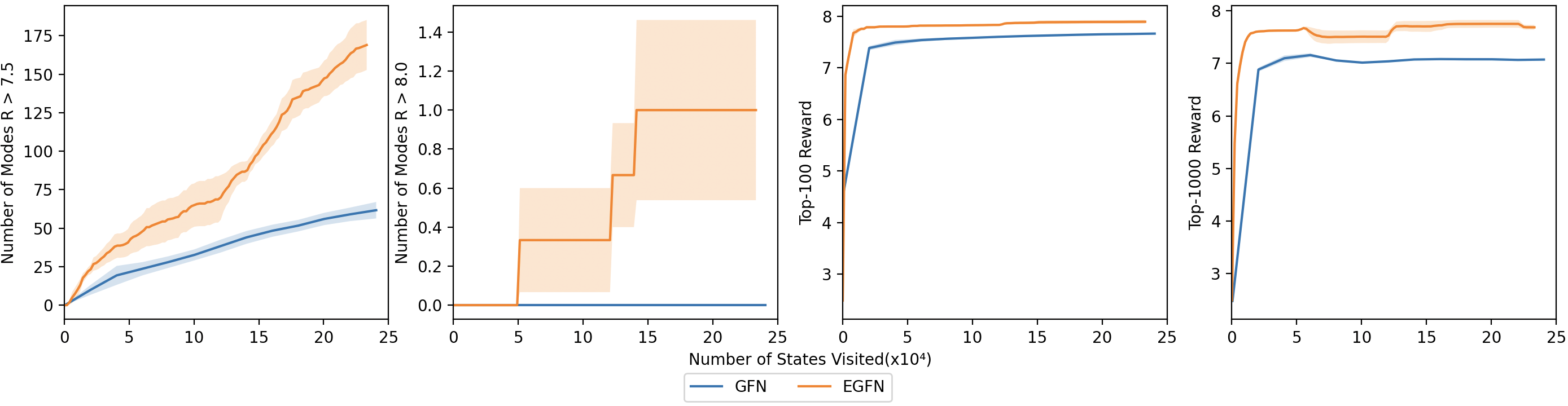
Figure 10: From left to right. (Example binder produced in the Soluable Epoxy Hydrolase (sEH)binder generation task. Here the structure corresponds to the molecule with SMILES representation O=P([O-])(O)c1ccc2ccccc2c1. sEH binder generation experiment over $2.5\times 10^{4}$ training steps. GFlowNets implementation uses FM objective. The number of modes with a reward threshold of 7.5 and 8.0. The average reward across the top-100 and 1000 molecules. The proposed augmentation with EGFN achieves better results both in terms of mode discovery and average reward.

5 Discussion

Why does EGFN work? To explore this, we compare the trajectories stored in the training step for GFlowNets and EGFN across training steps $\in\{500,1000,1500,2000,2500\}$ in the hypergrid task in figure 9 for different levels of sparsity ($R_{0}\in\{10^{-2},10^{-5}\}$). We see that when reward sparsity is low (left), training trajectory length distribution of both methods is similar. However, when the reward sparsity increases (right), GFlowNets training trajectories center around a lower trajectory length than that of EGFN. However, for a reward-symmetrical environment like hypergrid, the trajectory length’s distribution must tend towards the mean to truly capture the data distribution. EGFN can achieve this by its reward-maximizing evolutionary process which supplies diverse modes to the PRB, ensuring a better training for the star agent.

6 Related work

6.1 Evolution in learning

There has been many attempts to augment learning, especially RL, with EA. Early works such Whiteson (2006) combine NEAT (Stanley & Miikkulainen, 2002a) and Q Learning (Watkins & Dayan, 1992) by using evolutionary strategies to better tune the function approximators. In a similar manner, Colas et al. (2018) uses EA for exploration in policy gradient, generating diverse samples using mutation. Fernando et al. (2017) use EA for allowing parameter reuse without catastrophic forgetting. Recently, many methods use EA to enhance deep RL architectures such as Proximal Policy Optimization (PPO)(Hämäläinen et al., 2020), Soft-Actor Critic (SAC)(Hou et al., 2020), and Policy Gradient (Khadka & Tumer, 2018). The key idea from these approaches is to use EA to overcome the temporal credit assignment and improve exploration by getting diverse samples (Lee et al., 2020), with some exceptions such as Gangwani & Peng (2018); Fujimoto et al. (2018); Pourchot & Sigaud (2019) where they utilize EA to tune the parameter of the actor itself.

6.2 GFlowNets

GFlowNets have recently been applied to various problems (Liu et al., 2023; Bengio et al., 2021). There have also been recent efforts in extending GFlowNets to continuous (Lahlou et al., 2023) and stochastic worlds (Pan et al., 2023b), and also leveraging the power of pre-trained models (Pan et al., 2024). In GFlowNets training, exploration is an important concept for training convergence, which many works attempt in different ways. For example, Bengio et al. (2021) use $\epsilon$-greedy exploration strategy, Kim et al. (2023) learn the logits conditioned on different annealed temperatures, Pan et al. (2022b) introduces augmented flows into the flow network represented by intrinsic rewards, etc. The temporal credit assignment for long trajectories and sparse reward is a more recently studied topic for GFlowNets. Recent works such as Malkin et al. (2022) attempt to tackle this problem by minimizing the loss over an entire trajectory as opposed to state-wise FM proposed by Bengio et al. (2021), however, it may incur large variance as demonstrated in Madan et al. (2023).

7 Conclusion

In this work, we presented EGFN, a simple but effective augmentation EA strategy for training GFlowNets, especially for credit assignment in long trajectories and sparse rewards. This strategy mixes the best of both worlds: EA’s population-based approach biases towards regions with long-term returns, and GFlowNet’s gradient-based objectives handle the matching of the reward distribution with the sample distribution by leveraging better gradient signals. Besides, EA promotes natural diversity of the explored region, removing the need to use any other exploration strategies for GFlowNets training. Furthermore, by incorporating PRB for offline samples, EA promotes redundancy of high region samples, stabilizing the GFlowNet training with better gradient signals. We validate our method on a wide range of challenging toy and real-world benchmarks with exponentially large combinatorial search spaces, showing that our method outperforms the best GFlowNet baselines on long time horizon and sparse rewards.

In this work, we implement a standard evolutionary algorithm for EGFN. Incorporating more complex sub-modules of EA for GFlowNets training such as Covariance Matrix Adaptation and Evolution Strategy (CMA-ES) such as the work in Pourchot & Sigaud (2019) can be an exciting future work. Another future direction could be integrating the gradient signal from the GFlowNets objectives into the EA strategy, creating a feedback loop. Besides, while we use a reward-maximization formulation for the EA in this work, there are works such as Parker-Holder et al. (2020) that directly improves diversity by formulation. We leave that for the future work.

Impact statement

The primary goal of this work is to advance the field of Machine Learning. The authors, thus, do not foresee any specfic negative impacts of this work.

Appendix A Reproducibility

Our code is available at https://anonymous.4open.science/r/E-GFN/. The hypergrid and sEH binder task is based on the code from https://github.com/zdhNarsil/Distributional-GFlowNets. The QM9 and TFBind8 task is based on the code from https://github.com/maxwshen/gflownet. All our implementation code uses the PyTorch library (Paszke et al., 2019). We used MolView https://molview.org/ to visualize the molecule diagrams for our paper.

Appendix B Summary of notations

We summarize the notations used in our paper in the table 1 below.

Table 1: Notations summary

Symbol	Description
$\mathcal{S}$	state space
$\mathcal{X}$	terminal state space
$\mathcal{A}$	action space ($s\rightarrow s^{\prime}$)
$\mathcal{T}$	trajectory space
$s_{0}$	initial state in $\mathcal{S}$
$s$	state in $\mathcal{S}$
x	terminal state in $\mathcal{X}$
$\tau$	trajectory in $\mathcal{T}$
$P_{F}$	forward flow
$P_{B}$	backward flow
$k$	population size
$\mathcal{D}$	replay buffer
$\epsilon$	elite population ratio
$\gamma$	mutation strength

Appendix C Fitness evaluation algorithm

Algorithm 2 Evaluation of Forward Flows

Data: Forward flow $P_{F}$

Result: Updated replay buffer with trajectories and fitness of $P_{F}$

Procedure EVALUATE($P_{F},\mathcal{E},\mathcal{D}$)

       fitness $\leftarrow$ 0
for $iter$ = 1 to $\mathcal{E}$ do

             Initialize start state $s$ ;

              // Can also be parallelized Initialize trajectory $\mathcal{T}$ to an empty list
while $s$ not a terminal state do

                   Sample action $a$ based on $P_{F}(s|\theta_{P_{F}})$
$s^{\prime}\leftarrow transition(s,a)$
Append $(s^{\prime},a)$ to the $\mathcal{T}$
$s\leftarrow s^{\prime}$

            Compute $\mathcal{R}$(s) using reward function using the last state in $\mathcal{T}$
Append $\mathcal{T}$ to $\mathcal{D}$

      Return $\frac{\text{fitness}}{\mathcal{E}}$, $\mathcal{D}$

Appendix D Additional implementation details

D.1 Hypergrid task

The hypergrid reward function is defined by -

$$R(\texttt{x})=R_{0}+R_{1}\prod_{d=1}^{D}{\mathbb{I}\left[\left|\frac{\texttt{x}_{d}}{H-1}-0.5\right|\in\left(0.25,0.5\right]\right]}+R_{2}\prod_{d=1}^{D}{\mathbb{I}\left[\left|\frac{\texttt{x}_{d}}{H-1}-0.5\right|\in\left(0.3,0.4\right]\right]}$$ (6)

where $\mathbb{I}$ is the indicator function and $R_{0},R_{1},$ and $R_{2}$ are reward control parameters. In our experiments, $R_{1}$ and $R_{2}$ stay at a fixed value of 0.5 and 2. In our experiments, $R_{0}$ varies within $\{10^{-3},10^{-4},10^{-5}\}$. A mode is the terminal state x for which $R(\texttt{x})=R_{max}$. From the equation 6, it is evident that there are $2^{D}$ distinct modes. Besides, $H$ refers to the horizon of the environment, meaning each dimension of x can be equal to $i\in\{0,1,2,\dots,H-1\}$. For example, figure 5 uses $D=5$ and $H=20$. Clearly, while increasing both $D$ and $H$ increases the complexity of the task, effecting the trajectory length $|\tau|$ and the number of states $|\mathcal{X}|$, only increasing $D$ increases the number of modes. To calculate the empirical probability density, we collect the past visited 200000 states and calculate the probability density.

Architecture We model the forward layer with a 3-layer MLP with 256 hidden dimensions, followed by a leaky ReLU. The forward layer takes the one-hot encoding of the states as inputs and outputs action logits. For FM, we simply use the forward layer to model the edge flow. For TB and DB, we double the action space and train the MLP as both the forward and backward flow. We use a learning rate of $10^{-4}$ for FM and $10^{-3}$ for both TB and DB, including a learning rate of 0.1 for $Z_{\theta}$. The replay buffer uses a maximum size of 1000, and we use a worst-reward first policy for replay replacement.

D.2 sEH binder generation Task

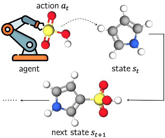
Figure 11: Illustration of GFlowNets policy for sEH binder generation task. Figure adopted from Pan et al. (2022a)

For this task, the number of actions is within 100 to 2000, depending on the state, making $|\mathcal{X}|\approx 10^{16}$. We allow the agent to choose from a library of 72 blocks. Similar to Bengio et al. (2021), we include the different symmetry groups of a given block, making the action count 105 per stem. We also allow the agent to select up to 8 blocks, choosing them as suggested by (Sterling & Irwin, 2015) from the ZINC dataset (Sterling & Irwin, 2015). Following Zhang et al. (2023b), we use Tanimoto similarity, defined by the ratio between the intersection and the union of two molecules based on their SMILES representation. To maintain diversity, we define a mode to be a terminal state for which the normalized negative binding energy to the 4JNC inhibitor of the soluble epoxide hydrolase (sEH) protein is more than 7.5 and the tanimoto similarity of other discovered modes is less than 0.7. Note that this objective is more limiting than simply counting the number of different Bemis-Murcko scaffolds that reach the reward threshold like Bengio et al. (2021). Since we are focusing on both molecule separation and optimization, our approach is more applicable for de novo molecule design, while the scaffold-based metric is suitable for lead optimization.

Architecture Following Bengio et al. (2021), we use a message passing neural network (MPNN)(Gilmer et al., 2017) that receives the atom graph to calculate the proxy reward of the molecules. Similarly, we use another MPNN that receives the block graph for flow estimation. The block graph is a tree of learned node embeddings that represent the blocks and edge embeddings that represent the bonds. To represent the flow, we pass the stems through a 10-layer graph convolution followed by GRU to calculate their embedding and pass the embedding through a 3-layer MLP to get a 105-dimension logit. Similarly, to represent the stop action, we pass the global mean pooling to the 3-layer MLP. The MLPs use 256 hidden dimensions, followed by a leakyReLU. We use a learning rate of 0.0005 and a minibatch size of 4. For EGFN, we use an offline sample probability of 0.2. Besides, we use a reward exponent $\beta$ = 10 and a normalizing constant of 8. For RL and MCMC baselines, we use the implementation provided by Bengio et al. (2021).

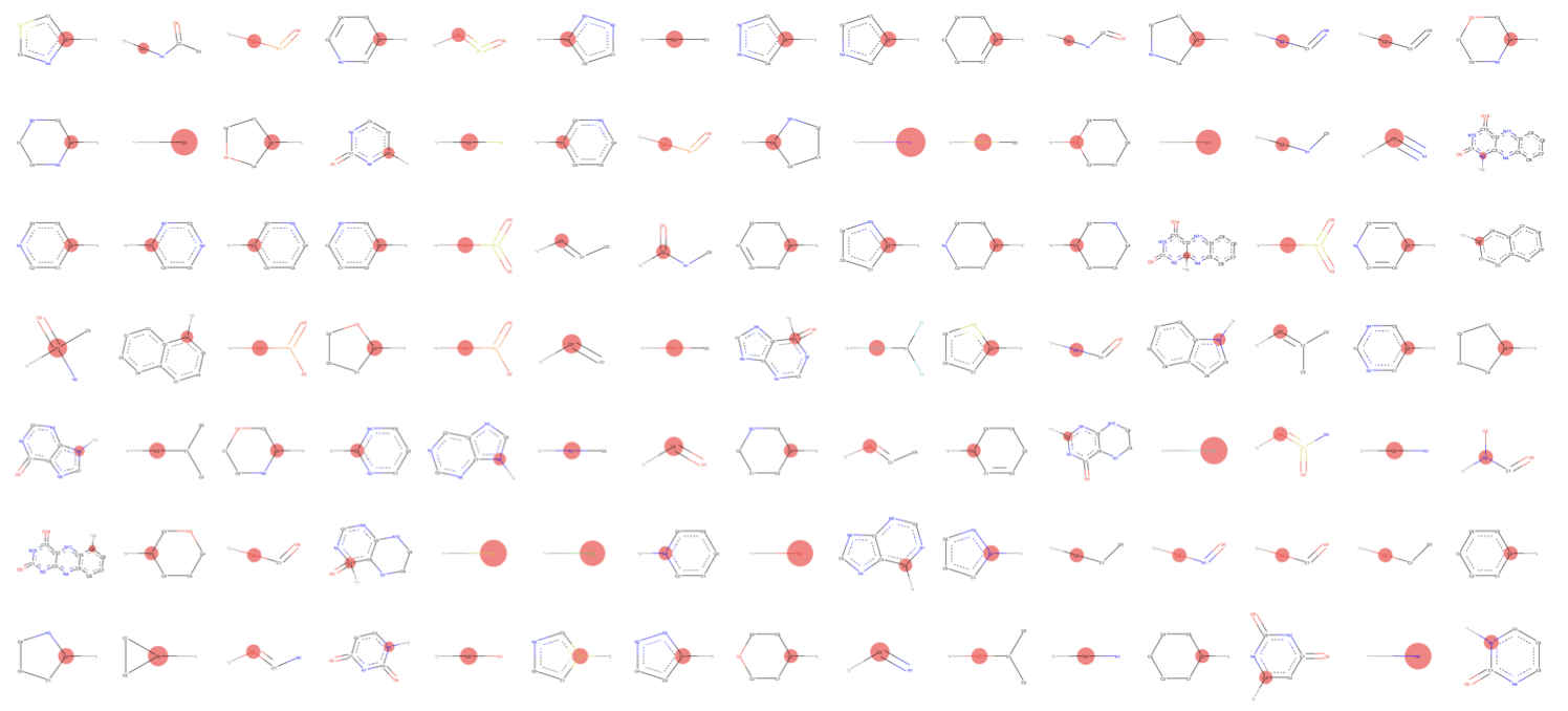
Figure 12: Molecule blocks for the sEH protein task. Figure adapted from Bengio et al. (2021)

D.3 TFBind8 task

For this task, the goal is to generate an 8-length DNA sequence that maximizes the binding activity score with a particular transcription factor SIX6REFR1 (Barrera et al., 2016). We use a precalculated oracle for the proxy reward calculation. Using a PA-MDP, we prepend or append a neucleotide in each step. Note that this formulation reduces the trajectory length significantly despite our effort to showcase better performance in long trajectories, but we use it following previous works.

Architecture Following (Shen et al., 2023), the GFlowNets architecture uses a 2-layer MLP with 128-dimension hidden layer parameterizing SSR ($\mathcal{S},\mathcal{S^{\prime}}\rightarrow\mathbb{R}^{+}$). For each training step, we train on both online and offline trajectories for three steps, using a minibatch of 32. Besides, we use a learning rate of $10^{-4}$ for policy and $0.01$ for $Z_{\theta}$. Finally, we use a reward exponent $\beta$ = 3 and an exploration probability of 0.01 (we do not use any exploration for EGFN).

D.4 QM9 task

The goal here is to generate diverse molecules based on the QM9 data (Ramakrishnan et al., 2014) that maximize the HOMO-LUMO. To that end, we use the reward proxy that Jain et al. (2023b) provides based on Zhang et al. (2020). Similar to the sEH task, we generate molecules with atoms and bonds. The blocks used here are the following: C, 0, N, C-F, C=0, C#C, c1ccccc1, C1CCCCC1, C1CCNC1, CCC.

Architecture Using a PA-MDP, we use a 2-layer MLP with 1024 hidden dimensions for flow estimation. The reward proxy is a MXMNet proxy trained on the QM9 data. We use a reward exponent $\beta=1$. The learning rate and training style follow the ones used for the TFBind8 task, with the exception of exploration probability (0.1 here) and hidden dimension (1024 here).

We detail the summary of the training hyperparameters in table 2.

Table 2: Summary of the hyperparameters for all experiments

	Hypergrid	sEH Small Molecules	TFBind8	QM9
Learning Rate	$10^{-4}$ (FM), $10^{-3}$	$5\times 10^{-4}$	$10^{-4}$	$10^{-4}$
$Z_{\theta}$ Learning Rate	0.1	N/A	0.01	0.01
$\beta$	1	10	3	1
MDP	Enumerate	Sequence Insert	PA-MDP	PA-MDP
Exploration $\epsilon$ (none for EGFN)	0	0	0.01	0.1
Replay Buffer Training	50%	0 (20% for egfn)	50%	50%
MLP layers	3	3	2	2
MLP hidden dimensions	256	256	128	1024

Appendix E Additional ablation experiments

E.1 Number of population

To investigate the effect of population size, we vary the $k\in$ $\{5,10,15\}$, while keeping $\epsilon=0.2,D=5,H=20,R_{0}=10^{-5}$. We plot the results of the experiment in figure 13. It shows that increasing $k$ beyond 10 leads to diminishing returns, motivating our choice of $k=10$ for all the experiments. For DB, however, increasing $k$ leads to considerable improvement. Indeed, this is useful because increased population size leads to more evaluation round required. While these evaluation round can be parallelized with threads as we do in our work, massive population size requirement is difficult to satisfy.

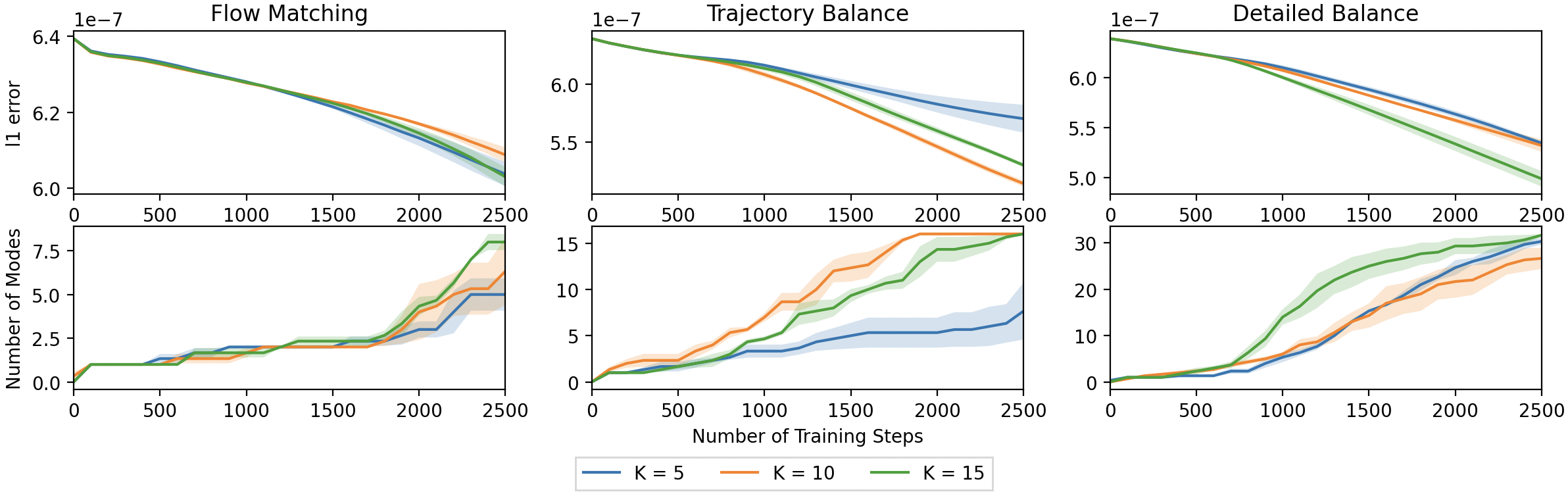
Figure 13: Experimental results for the hypergrid task for EGFN among different values of $k$ across the three training objectives. Top: the $\ell_{1}$ error between the learned distribution density and the true target density. Bottom: the number of discovered modes across the training process. Here, $H=20,D=5$. The results show that increasing population size leads to diminishing returns.

E.2 Elite population

Following ablation on $k$, we next perform ablation on the elite population ratio, $\epsilon\in\{0.2,0.4,0.6\}$. For this experiment, we use the same hypergrid settings for $k=10$. We plot the results of the experiment in figure 14. It shows that low $\epsilon$ improves mode discovery, especially for FM and TB objectives. This result is reasonable: we apply mutation and crossover only to the non-elite population, so having a low number of elite population means we have a better chance at exploring using the non-elite population’s mutation and crossover.

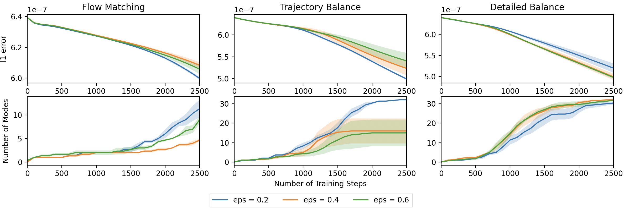
Figure 14: Experimental results for the hypergrid task for EGFN among different values of $\epsilon$ across the three training objectives. Top: the $\ell_{1}$ error between the learned distribution density and the true target density. Bottom: the number of discovered modes across the training process. Here, $H=20,D=5$. We observe that lower $\epsilon$ leads to better results for FM and TB.

E.3 Replay buffer size

To understand the effect of replay buffer size, we run GFlowNets baseline with PRB and EGFN on a 20x20x20x20x20 environment with $R_{0}=10^{-5}$ for replay buffer size $\in\{1000,5000,10000\}$. We present the findings in figure 15. From the figure, we see that increasing buffer size generally has little effect for GFlowNets, but it improves EGFN’s robustness a little.

Figure 15: Experimental results for the hypergrid task between GFlowNets and EGFN across different values of $|\mathcal{D}|$. Top: the $\ell_{1}$ error between the learned distribution density and the true target density. Bottom: the number of discovered modes across the training process. Here, we use DB for $H=20,D=5$. The results show that while increasing replay buffer size improves the robustness of the result, it has little effect otherwise.

E.4 Mutation strength

We now turn our attention to the mutation. To observe the effect of the mutation strength $\gamma$, we run the hypergrid experiment for the three training objectives using EGFN for $\gamma\in{1,5,10}$. The hypergrid configurations follow the the same configurations as before. We plot the mode discovery and $\ell_{1}$ error between the learned distribution density and the true target density over 2500 training steps in figure 16. While the results indicate that having a higher $\gamma$ leads to better result for DB, the improvement is not extraordinary. Besides, in our work, we experience training instability for higher $\gamma$. Thus, we restrict $\gamma$ to be 1 throughout in our work.

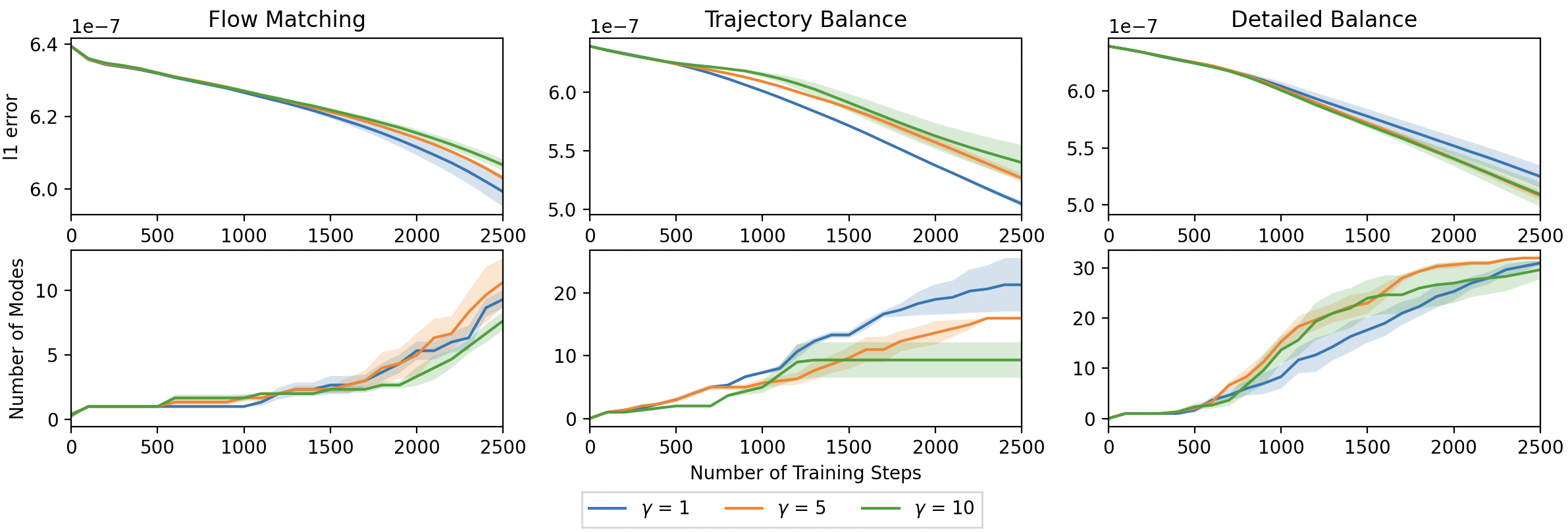
Figure 16: Experimental results for the hypergrid task for EGFN among different values of $\gamma$ across the three training objectives. Top: the $\ell_{1}$ error between the learned distribution density and the true target density. Bottom: the number of discovered modes across the training process. Here, $H=20,D=5$. We observe that lower $\gamma$ leads to better results for FM and TB, while higher $\gamma$ leads to better results for DB.

References

- Bäck (2006) Bäck, T. Evolutionary computation: Toward a new philosophy of machine intelligence (ieee press series on computational intelligence). 2006. URL https://api.semanticscholar.org/CorpusID:27611267.
- Bäck & Schwefel (1993) Bäck, T. and Schwefel, H.-P. An overview of evolutionary algorithms for parameter optimization. Evolutionary computation, 1(1):1–23, 1993.
- Barrera et al. (2016) Barrera, L. A., Vedenko, A., Kurland, J. V., Rogers, J. M., Gisselbrecht, S. S., Rossin, E. J., Woodard, J., Mariani, L., Kock, K. H., Inukai, S., et al. Survey of variation in human transcription factors reveals prevalent dna binding changes. Science, 351(6280):1450–1454, 2016.
- Bengio et al. (2021) Bengio, E., Jain, M., Korablyov, M., Precup, D., and Bengio, Y. Flow network based generative models for non-iterative diverse candidate generation. Advances in Neural Information Processing Systems, 34:27381–27394, 2021.
- Bengio et al. (2023) Bengio, Y., Lahlou, S., Deleu, T., Hu, E. J., Tiwari, M., and Bengio, E. Gflownet foundations. Journal of Machine Learning Research, 24(210):1–55, 2023.
- Bickerton et al. (2012) Bickerton, G. R., Paolini, G. V., Besnard, J., Muresan, S., and Hopkins, A. L. Quantifying the chemical beauty of drugs. Nature chemistry, 4(2):90–98, 2012.
- Christodoulou (2019) Christodoulou, P. Soft actor-critic for discrete action settings. arXiv preprint arXiv:1910.07207, 2019.
- Colas et al. (2018) Colas, C., Sigaud, O., and Oudeyer, P.-Y. Gep-pg: Decoupling exploration and exploitation in deep reinforcement learning algorithms. In International conference on machine learning, pp. 1039–1048. PMLR, 2018.
- Fernando et al. (2017) Fernando, C., Banarse, D., Blundell, C., Zwols, Y., Ha, D., Rusu, A. A., Pritzel, A., and Wierstra, D. Pathnet: Evolution channels gradient descent in super neural networks. arXiv preprint arXiv:1701.08734, 2017.
- Floreano et al. (2008) Floreano, D., Dürr, P., and Mattiussi, C. Neuroevolution: from architectures to learning. Evolutionary Intelligence, 1:47–62, 2008. URL https://api.semanticscholar.org/CorpusID:2942634.
- Fujimoto et al. (2018) Fujimoto, S., Hoof, H., and Meger, D. Addressing function approximation error in actor-critic methods. In International conference on machine learning, pp. 1587–1596. PMLR, 2018.
- Gangwani & Peng (2018) Gangwani, T. and Peng, J. Policy optimization by genetic distillation. In International Conference on Learning Representations, 2018.
- Gilmer et al. (2017) Gilmer, J., Schoenholz, S. S., Riley, P. F., Vinyals, O., and Dahl, G. E. Neural message passing for quantum chemistry. In International conference on machine learning, pp. 1263–1272. PMLR, 2017.
- Haarnoja et al. (2018) Haarnoja, T., Zhou, A., Abbeel, P., and Levine, S. Soft actor-critic: Off-policy maximum entropy deep reinforcement learning with a stochastic actor. In International conference on machine learning, pp. 1861–1870. PMLR, 2018.
- Hämäläinen et al. (2020) Hämäläinen, P., Babadi, A., Ma, X., and Lehtinen, J. Ppo-cma: Proximal policy optimization with covariance matrix adaptation. In 2020 IEEE 30th International Workshop on Machine Learning for Signal Processing (MLSP), pp. 1–6. IEEE, 2020.
- Hou et al. (2020) Hou, Z., Zhang, K., Wan, Y., Li, D., Fu, C., and Yu, H. Off-policy maximum entropy reinforcement learning: Soft actor-critic with advantage weighted mixture policy (sac-awmp). arXiv preprint arXiv:2002.02829, 2020.
- Ikram et al. (2023) Ikram, Z., Pan, L., and Liu, D. Probabilistic generative modeling for procedural roundabout generation for developing countries. In NeurIPS 2023 Workshop on Adaptive Experimental Design and Active Learning in the Real World, 2023. URL https://openreview.net/forum?id=WWqJWiyQ2D.
- Jain et al. (2022) Jain, M., Bengio, E., Hernandez-Garcia, A., Rector-Brooks, J., Dossou, B. F., Ekbote, C. A., Fu, J., Zhang, T., Kilgour, M., Zhang, D., et al. Biological sequence design with gflownets. In International Conference on Machine Learning, pp. 9786–9801. PMLR, 2022.
- Jain et al. (2023a) Jain, M., Deleu, T., Hartford, J., Liu, C.-H., Hernandez-Garcia, A., and Bengio, Y. Gflownets for ai-driven scientific discovery. Digital Discovery, 2(3):557–577, 2023a.
- Jain et al. (2023b) Jain, M., Raparthy, S. C., Hernández-Garcıa, A., Rector-Brooks, J., Bengio, Y., Miret, S., and Bengio, E. Multi-objective gflownets. In International Conference on Machine Learning, pp. 14631–14653. PMLR, 2023b.
- Khadka & Tumer (2018) Khadka, S. and Tumer, K. Evolution-guided policy gradient in reinforcement learning. In Neural Information Processing Systems, 2018. URL https://api.semanticscholar.org/CorpusID:53096951.
- Kim et al. (2023) Kim, M., Ko, J., Zhang, D., Pan, L., Yun, T., Kim, W. C., Park, J., and Bengio, Y. Learning to scale logits for temperature-conditional gflownets. In NeurIPS 2023 AI for Science Workshop, 2023.
- Lahlou et al. (2023) Lahlou, S., Deleu, T., Lemos, P., Zhang, D., Volokhova, A., Hernández-Garcıa, A., Ezzine, L. N., Bengio, Y., and Malkin, N. A theory of continuous generative flow networks. In International Conference on Machine Learning, pp. 18269–18300. PMLR, 2023.
- Lee et al. (2020) Lee, K., Lee, B.-U., Shin, U., and Kweon, I. S. An efficient asynchronous method for integrating evolutionary and gradient-based policy search. Advances in Neural Information Processing Systems, 33:10124–10135, 2020.
- Liu et al. (2023) Liu, D., Jain, M., Dossou, B. F., Shen, Q., Lahlou, S., Goyal, A., Malkin, N., Emezue, C. C., Zhang, D., Hassen, N., et al. Gflowout: Dropout with generative flow networks. In International Conference on Machine Learning, pp. 21715–21729. PMLR, 2023.
- Lüders et al. (2017) Lüders, B., Schläger, M., Korach, A., and Risi, S. Continual and one-shot learning through neural networks with dynamic external memory. In EvoApplications, 2017. URL https://api.semanticscholar.org/CorpusID:37413014.
- Madan et al. (2023) Madan, K., Rector-Brooks, J., Korablyov, M., Bengio, E., Jain, M., Nica, A. C., Bosc, T., Bengio, Y., and Malkin, N. Learning gflownets from partial episodes for improved convergence and stability. In International Conference on Machine Learning, pp. 23467–23483. PMLR, 2023.
- Malkin et al. (2022) Malkin, N., Jain, M., Bengio, E., Sun, C., and Bengio, Y. Trajectory balance: Improved credit assignment in gflownets. Advances in Neural Information Processing Systems, 35:5955–5967, 2022.
- Pan et al. (2022a) Pan, L., Zhang, D., Courville, A., Huang, L., and Bengio, Y. Generative augmented flow networks. In The Eleventh International Conference on Learning Representations, 2022a.
- Pan et al. (2022b) Pan, L., Zhang, D., Courville, A., Huang, L., and Bengio, Y. Generative augmented flow networks. In The Eleventh International Conference on Learning Representations, 2022b.
- Pan et al. (2023a) Pan, L., Malkin, N., Zhang, D., and Bengio, Y. Better training of gflownets with local credit and incomplete trajectories. arXiv preprint arXiv:2302.01687, 2023a.
- Pan et al. (2023b) Pan, L., Zhang, D., Jain, M., Huang, L., and Bengio, Y. Stochastic generative flow networks. arXiv preprint arXiv:2302.09465, 2023b.
- Pan et al. (2024) Pan, L., Jain, M., Madan, K., and Bengio, Y. Pre-training and fine-tuning generative flow networks. In The Twelfth International Conference on Learning Representations, 2024. URL https://openreview.net/forum?id=ylhiMfpqkm.
- Parker-Holder et al. (2020) Parker-Holder, J., Pacchiano, A., Choromanski, K. M., and Roberts, S. J. Effective diversity in population based reinforcement learning. Advances in Neural Information Processing Systems, 33:18050–18062, 2020.
- Paszke et al. (2019) Paszke, A., Gross, S., Massa, F., Lerer, A., Bradbury, J., Chanan, G., Killeen, T., Lin, Z., Gimelshein, N., Antiga, L., et al. Pytorch: An imperative style, high-performance deep learning library. Advances in neural information processing systems, 32, 2019.
- Pourchot & Sigaud (2019) Pourchot, A. and Sigaud, O. Cem-rl: Combining evolutionary and gradient-based methods for policy search. In 7th International Conference on Learning Representations, ICLR 2019, 2019.
- Ramakrishnan et al. (2014) Ramakrishnan, R., Dral, P. O., Rupp, M., and Von Lilienfeld, O. A. Quantum chemistry structures and properties of 134 kilo molecules. Scientific data, 1(1):1–7, 2014.
- Rector-Brooks et al. (2023) Rector-Brooks, J., Madan, K., Jain, M., Korablyov, M., Liu, C.-H., Chandar, S., Malkin, N., and Bengio, Y. Thompson sampling for improved exploration in gflownets. In ICML 2023 Workshop on Structured Probabilistic Inference & Generative Modeling, 2023.
- Risi & Togelius (2014) Risi, S. and Togelius, J. Neuroevolution in games: State of the art and open challenges. IEEE Transactions on Computational Intelligence and AI in Games, 9:25–41, 2014. URL https://api.semanticscholar.org/CorpusID:11245845.
- Schulman et al. (2017) Schulman, J., Wolski, F., Dhariwal, P., Radford, A., and Klimov, O. Proximal policy optimization algorithms. arXiv preprint arXiv:1707.06347, 2017.
- Shen et al. (2023) Shen, M. W., Bengio, E., Hajiramezanali, E., Loukas, A., Cho, K., and Biancalani, T. Towards understanding and improving gflownet training. arXiv preprint arXiv:2305.07170, 2023.
- Shi et al. (2020) Shi, C., Xu, M., Guo, H., Zhang, M., and Tang, J. A graph to graphs framework for retrosynthesis prediction. In International conference on machine learning, pp. 8818–8827. PMLR, 2020.
- Spears et al. (1993) Spears, W. M., Jong, K. A. D., Bäck, T., Fogel, D. B., and de Garis, H. An overview of evolutionary computation. In European Conference on Machine Learning, 1993. URL https://api.semanticscholar.org/CorpusID:175549.
- Stanley & Miikkulainen (2002a) Stanley, K. O. and Miikkulainen, R. Evolving neural networks through augmenting topologies. Evolutionary computation, 10(2):99–127, 2002a.
- Stanley & Miikkulainen (2002b) Stanley, K. O. and Miikkulainen, R. Evolving neural networks through augmenting topologies. Evolutionary Computation, 10:99–127, 2002b. URL https://api.semanticscholar.org/CorpusID:498161.
- Sterling & Irwin (2015) Sterling, T. and Irwin, J. J. Zinc 15–ligand discovery for everyone. Journal of chemical information and modeling, 55(11):2324–2337, 2015.
- Trabucco et al. (2022) Trabucco, B., Geng, X., Kumar, A., and Levine, S. Design-bench: Benchmarks for data-driven offline model-based optimization. In International Conference on Machine Learning, pp. 21658–21676. PMLR, 2022.
- Watkins & Dayan (1992) Watkins, C. J. and Dayan, P. Q-learning. Machine learning, 8:279–292, 1992.
- Whiteson (2006) Whiteson, S. Evolutionary function approximation for reinforcement learning. Journal of Machine Learning Research, 7, 2006.
- Xie et al. (2020) Xie, Y., Shi, C., Zhou, H., Yang, Y., Zhang, W., Yu, Y., and Li, L. Mars: Markov molecular sampling for multi-objective drug discovery. In International Conference on Learning Representations, 2020.
- Zhang et al. (2023a) Zhang, D., Dai, H., Malkin, N., Courville, A., Bengio, Y., and Pan, L. Let the flows tell: Solving graph combinatorial problems with gflownets. In Thirty-seventh Conference on Neural Information Processing Systems, 2023a.
- Zhang et al. (2023b) Zhang, D., Pan, L., Chen, R. T., Courville, A., and Bengio, Y. Distributional gflownets with quantile flows. arXiv preprint arXiv:2302.05793, 2023b.
- Zhang et al. (2020) Zhang, S., Liu, Y., and Xie, L. Molecular mechanics-driven graph neural network with multiplex graph for molecular structures. arXiv preprint arXiv:2011.07457, 2020.
- Zhao et al. (2019) Zhao, R., Sun, X., and Tresp, V. Maximum entropy-regularized multi-goal reinforcement learning. In International Conference on Machine Learning, pp. 7553–7562. PMLR, 2019.