Phase space eigenfunctions with applications to continuum kinetic simulations

Abstract

Fully kinetic simulations utilizing finite element methods or structure-preserving particle-in-cell methods are becoming increasingly sophisticated and capable of resolving analytic features in high-dimensional phase space. These capabilities can be more fully explored by using linear kinetic theory to initialize the phase space mode structures corresponding to the modes of oscillation and instability in model problems and benchmarking. Phase space eigenfunctions typically have a fairly simple analytic form, or in some cases may be sufficiently well approximated by truncation of a cyclotron-harmonic expansion. This article explores the phase space eigenfunctions of linear kinetic theory in their simplest manifestations for homogeneous plasmas, and illustrates their practical application by simulation of single- and multi-mode instabilities evolving into nonlinear structures for the prototypical streaming instability, loss-cone instability, and Weibel instability problems. Other applications of the linear kinetic modes are noted, namely their utility as the underlying actors in the spectra predicted by quasilinear kinetic theories.

1 Introduction

Plasma kinetic simulations shed light on fundamental dynamics and make up a perennial topic in the literature (Bertrand and Feix, (1968); Cheng and Knorr, (1976); Birdsall and Langdon, (1991); Heath et al., (2012); Morrison, (2017)). As a well-known example of such fundamental behavior, a plasma in macroscopic equilibrium yet away from thermal equilibrium may be associated with unstable linear modes (Penrose, (1960)). The drive towards thermal equilibrium is a broad and general principle, so that one finds even in the simplest homogeneous plasmas numerous instability modes due to streaming, anisotropic pressure, loss-cones, etc. (Weibel, 1959a ; Rosenbluth and Post, (1965)). Put simply, the unstable phase space distribution functions are entropically unfavorable distributions of relative velocity. Kinetic instabilities are important to macroscopic dynamics through their relationship with resistivity and diffusion (Drummond and Rosenbluth, (1962); Yoon and Lui, (2006)), and many decades of kinetic simulations have supported theory to make substantial contributions in the dynamical sciences (Escande, (2016)) and in transport modeling for fluid closures (Conner and Wilson, (1994)). A huge potential remains for kinetic simulation to enrich plasma theory as advances in technique and computing power overcome the curse of dimensionality (He et al., (2016); Choi et al., (2021)).

Usually kinetic simulations solve the initial-value problem of a perturbed, unstable equilibrium probability distribution function $f_{0}$. The perturbation is constructed as a superposition of spatial modes with particle densities arising from a perturbed distribution $f_{1}$. To achieve these density perturbations the equilibrium is often perturbed as $f_{1}(x,v)=A\sin(kx)f_{0}(v)$. However, plasma modes consist of structure in both the field and the phase space self-consistently. Indeed, linear modes (namely, self-consistent plasma-field configurations) have a phase space structure more like $f_{1}(x,v)=(\zeta-v)^{-1}\partial_{v}f_{0}e^{ikx}$ with $\zeta=\omega/k$ a complex phase velocity, and so a significant portion of the perturbation energy is channeled into the Landau-damped modes and the model’s energy trace begins by a transient energetic reorganization via Landau damping. In other words, perturbations of the form $f_{1}=A\sin(kx)f_{0}(v)$ partition the perturbation energy in a manner different from what the researcher may have intended. The partition of energy into non-eigenfunction perturbations is okay when initial amplitudes are small, but at larger perturbation amplitude Landau damping may non-physically contribute to nonlinear phenomena as these modes are usually activated by thermal fluctuations. A numerical consideration arises when the perturbation contains both growing and damped modes of oscillation, in which case precise measurement of growth rates is obscured by Landau damping.

The objective of this article is to demonstrate that self-consistent plasma-field configurations can be specified and initialized using analytic expressions for the phase space eigenfunctions. The numerical and theoretical methods and results presented in this article will be of interest to researchers conducting kinetic simulations, whether by the particle-in-cell method (Barnes and Chacón, (2021)) or by the continuum finite element discretization (Heath et al., (2012); Einkemmer, (2019); Crews and Shumlak, (2022); Datta and Shumlak, (2023)). The methods of this article apply most directly to approaches where the perturbed distribution can be functionally specified in phase space. In our work we use a mixed Fourier spectral/finite element numerical method for continuum kinetic discretization discussed in Appendix A. However, it seems to the authors that sophisticated particle-in-cell methods can utilize these results and initialize eigenmode perturbations (Kraus et al., (2017); Glasser and Qin, (2020); Perse et al., (2021)).

This article is organized as theory followed by simulation, treating progressively the unmagnetized and magnetized electrostatic and unmagnetized electromagnetic problems. Section 2 reviews unmagnetized electrostatic phase space eigenfunctions and Landau modes, including a historical summary, a review of the initial-value problem, and an energetic analysis. Section 3 discusses the electrostatic cyclotron modes, making new connections to the theory of special functions for the dielectric tensor of loss cones regarding hypergeometric functions and the Laguerre polynomials, and notes the helical phase space structure of Bernstein modes. Section 4 considers the vector eigenmodes of the Vlasov-Maxwell system by casting the dielectric tensor as an eigenvalue problem for a system of integral equations over the equilibrium, and presents a method to obtain these modes. The natural consistency of the plasma-field configuration resulting from this method is observed as a benefit, so that the initial condition already satisfies Poisson’s equation, for example. That only instabilities occur as phase space eigenfunctions is generalized to the vector case, and the dielectric components of the bi-Maxwellian are explored in the context of Weibel instability. Illustrative simulations are presented in the relevant sections and include the multidimensional multi-mode two-stream instability in Section 2.7, single-mode Dory-Guest-Harris instability in Section 3.6, single-mode Weibel instability in Section 4.4, and multidimensional multi-mode Weibel problem in Section 4.5. The magnetized electromagnetic problem is not treated here, but we mention that simple analytic eigenfunctions do exist, such as the parallel-field whistler modes which involve only the first cyclotron harmonic. The linear theory for the electromagnetic problem can be found in Stix, (1992), for example.

2 Electrostatic plasma modes with zero-order ballistic trajectories

Perhaps the simplest problem in plasma kinetic theory is that of electrostatic modes in unmagnetized homogeneous plasma, meaning that the zero-order orbits are simply free-streaming ballistic motions. Here the problem is treated beginning with a historical discussion, followed by analysis of the initial-value problem, and an energetic analysis of response to eigenfunction and non-eigenfunction phase space perturbations. Recall that there are two ways of considering the linearized dynamics: the eigenvalue problem ($t\in(-\infty,\infty)$) and the initial-value problem ($t\in[0,\infty)$). A somewhat subtle theoretical point is the distinction between eigenfunctions and Landau-damped modes; to clarify this distinction requires a review of the Case-van Kampen modes and the theory of linear Landau damping, which can be found in Crews, (2022) and is omitted here for brevity. Nevertheless, in the following the distinction is reviewed at a qualitative level.

2.1 Historical summary and context

The study of eigenfunctions of collisionless and collisional plasma kinetic equations has a long history. Vlasov was the first to suggest a method to estimate the plasma oscillation frequencies by prescribing that the principal value be taken at the resonant velocity in the dispersion function. Following this Bohm and Gross, (1949) side-stepped the resonant term by considering high-enough phase velocities that the distribution function was effectively zero at the pole. Famously Landau, (1946) formally solved the linearized initial-value problem for Vlasov-Poisson dynamics using Laplace transformation, discovering a discrete set of solutions for the Maxwellian plasma, wherein the electric potential damped in time. This collisionless decay phenomenon is called Landau damping. For the collisionless plasma the decaying Landau modes are not eigenfunctions, meaning that such solutions cannot evolve independently. Yet Landau’s analysis also found unstable modes for certain distributions $f_{0}$. Thus, despite both unstable and dissipative modes sharing a similar phase space structure like $(v-\zeta)^{-1}\partial_{v}f_{0}e^{ikx}$, unstable modes evolve as a single analytic function while dissipation spreads across the entire Landau spectrum.

As the eigenvalue problem remained unsolved, van Kampen, (1955) and Case, (1959) formally solved the problem and determined the spectrum of the linearized kinetic equation to be continuous with a possibly discrete component. Discrete eigenvalues arise only for unstable modes where $\text{Im}(\omega)>0$. The continuous part of the spectrum consists of ballistic modes in the form $\varepsilon(k,\zeta)\delta(v-\zeta)$, while the discrete part in the analytic form $(v-\zeta)^{-1}\partial_{v}f_{0}$. Here $\varepsilon(k,\zeta)$ is the dielectric function and $f_{0}(v)$ the homogeneous equilibrium. The discrete part of the Case-van Kampen spectrum is identical to Landau’s unstable modes. Landau’s damping modes are represented as an integral expansion over the continuous Case-van Kampen spectrum. As a complete orthogonal system the Case-van Kampen modes are a useful though under-utilized tool. An insightful application was accomplished by P.J. Morrison and colleagues in constructing a linear integral transform, termed “G transform,” to reduce the linearized Vlasov equation to an advection problem by utilizing the Case-van Kampen modes as a basis (Morrison and Pfirsch, (1992); Morrison, (2000); Heninger and Morrison, (2018)).

As the Landau damping modes are not eigenfunctions their status has remained somewhat obscure. Light is shed on this problem by considering weak dissipation in the Vlasov equation, such as the collision operator of Lenard and Bernstein, (1958). It has been found numerically (Ng et al., (1999)) and analytically (Short and Simon, (2002)) that as dissipation tends to zero the dissipative eigenfunctions converge to the Landau damping modes, with the conclusion that dissipation is a singular perturbation of the collisionless dynamics. Bratanov et al., (2013) numerically confirmed this limit for discrete systems. However, the authors wish to highlight here that the Case-van Kampen modes still play a role in the dissipative picture. Namely, one can show (Bratanov et al., (2013); Crews, (2022)) that the propagator of the linearized kinetic equation with the Lenard-Bernstein operator limits to the Case-van Kampen modes as the dissipation $\nu\to 0^{+}$. This fact clarifies the relationship between the continuous Case-van Kampen spectrum and Landau damping modes, as even in the dissipative picture the Landau modes are represented as an integral over the diffusive propagator, and the collisionless Case-van Kampen modes indeed play the role of non-diffusive propagators (Balescu, (1997)). To understand why Landau modes are easily identified in the initial-value problem, consider that Landau damping originates from phase mixing (Mouhot and Villani, (2011)) and so the modes possess the peculiar property of decaying in both directions of time. Thus they arise by propagating initial data, or otherwise must be represented as an interference of free-streaming modes un-mixing from $t\in(-\infty,0)$ and re-mixing from $t\in(0,\infty)$.

In summary, in collisionless plasma kinetic theory unstable modes are normal modes and evolve independently, while dissipative modes either occur as a summation of non-orthogonal transient modes or must be represented in the Case-van Kampen spectrum. The Case-van Kampen spectrum has found fruitful application as the basis of constructing an integral transform theory for linearized dynamics, most recently explored in Heninger and Morrison, (2018). In weakly collisional dynamics dissipative modes are also eigenfunctions and limit to the collisionless Landau mode spectrum as dissipation tends to zero. As a consequence, it is possible to excite a single-mode instability by initializing its eigenfunction, but one may not excite a lone Landau-damping plane wave under collisionless dynamics. The following example illustrates this point.

2.2 Phase space linear response and the dielectric function

The electric susceptibility $\chi$ is the linear response function which relates in the spatiotemporal frequency domain $(\bm{x},t)\to(\bm{k},\omega)$ the polarization $\bm{\widetilde{P}}(\bm{k},\omega)$ and electric field $\bm{\widetilde{E}}(\bm{k},\omega)$ by the constitutive relation $\bm{\widetilde{P}}=\varepsilon_{0}\chi\bm{\widetilde{E}}$. In the scheme of electrostatic theory one aims to determine the susceptibility and consequently the dielectric permittivity $\varepsilon(\bm{k},\omega)=\varepsilon_{0}(1+\chi)$ of a plasma with equilibrium distribution $f_{0}(\bm{v})$. The susceptibility is determined through the self-consistent particle response $f_{1}(\bm{k},\bm{v},\omega)$ such that $f=f_{0}+f_{1}$, leading to the sought-after modal structures in the charge density. The distribution $f_{1}$ encodes a linear response of the charges to the electric potential $\varphi$ according to the relation $f_{1}=h(\bm{k},\bm{v},\omega)\varphi$ for some response function $h$. For this reason, we mean by “phase space linear response function” the self-consistent particle response $f_{1}$ to the potential $\varphi$. The permittivity is often referred to as simply the dielectric function because the permittivity tensor reduces to a scalar for isotropic equilibria.

The following review of the initial-value problem is done in detail for the simplest case in order to build intuition for the electromagnetic and magnetized problems where propagation of the initial data is tedious. Using the results, we then consider the evolution of perturbations in a plasma with Maxwellian $f_{0}$, namely a so-called Maxwellian perturbation (that is, where $f_{1}(x,v)=A\sin(kx)f_{0}(v)$) and a special pertubation describing a propagating, damping plane wave. When this plane wave is unstable the special pertubation grows as an eigenmode, i.e. a constant phase space structure with time-dependent amplitude, and when damped its structure evolves in phase space.

Rather than the usual Laplace transform notation, we use a more standard notation for the one-sided temporal Fourier transform pair as

$$f(\omega) =\int_{0}^{\infty}f(t)e^{i\omega t}dt,$$ (1)

$$f(t) =\frac{1}{2\pi}\int_{-\infty+is}^{\infty+is}f(\omega)e^{-i\omega t}d\omega$$ (2)

where the factor $s$ keeps the contour above all poles of the integrand in order that Eq. 1 converges. The contour in Eq. 2 is closed at infinity around the lower half-plane, and the inverse transform is then given by the residue theorem as

$$f(t)=-i\sum\text{Res}(f(\omega))$$ (3)

with the sum over all poles of the response function $f(\omega)$. The spatial Fourier transform $\bm{x}\to\bm{k}$ is defined as usual over all of space by $f(\bm{k})=\int d\bm{x}e^{-i\bm{k}\cdot\bm{x}}f(\bm{x})$. We consider for simplicity the response of a single species of particle charge $q$ and mass $m$ amidst a uniform neutralizing Maxwellian background, so we do not write a species subscript.

The Vlasov-Poisson system linearized by $f(\bm{x},\bm{v},t)=f_{0}+f_{1}$ with $f_{1}\ll f_{0}$ is given by

$$\frac{\partial f_{1}}{\partial t} +\bm{v}\cdot\nabla f_{1}-\frac{q}{m}(\nabla_{x}\varphi)\cdot\nabla_{v}f_{0}=0,$$ (4)

$$\nabla^{2}\varphi =-\frac{qn_{0}}{\varepsilon_{0}}\int f_{1}d\bm{v}.$$ (5)

Fourier transforming for all of space and for time $t\in(0,\infty)$ as described, the phase space linear response is obtained as

$$f_{1}(\bm{k},\bm{v},\omega)=i\frac{g(k,v)}{\omega-\bm{k}\cdot\bm{v}}-\frac{q}{m}\varphi\frac{\bm{k}\cdot\nabla_{v}f_{0}}{\omega-\bm{k}\cdot\bm{v}}.$$ (6)

where $g(k,v)=f_{1}(t=0,k,v)$ is the initial condition.

The following result is as described in Landau, (1946) with some change in notation. Define the Cauchy integral $g^{*}(k,\zeta)\equiv\int_{\mathcal{C}}\frac{g(k,v)}{\zeta-v}dv$, with $\mathcal{C}$ Landau’s contour (that is, analytically-continued into the lower-half $\zeta$-plane). Choose the coordinates such that one axis aligns with the wavevector $\bm{k}$, so that when computing the zeroth velocity moment of $f_{1}$, two of the velocity coordinates integrate out. The potential is found to be

$$\varphi(k,\zeta)=i\frac{\sigma}{k^{3}}\frac{g^{*}(k,\zeta)}{\varepsilon(k,\zeta)}$$ (7)

where $\sigma=q/|q|$ and $\varepsilon(k,\zeta)=1+k^{-2}\int_{\mathcal{C}}\frac{1}{\zeta-v}\frac{\partial f_{0}}{\partial v}dv$ is the electrostatic dielectric function. Here the wavenumber $k$ is normalized to the Debye length. If each root $\zeta_{j}$ of $\varepsilon(k,\zeta)=0$ is simple and $g^{*}(k,\zeta)$ has no poles then inverse transforming in time gives

$$\varphi(k,t)=\frac{\sigma}{k^{3}}\sum_{j}\frac{g^{*}(k,\zeta_{j})}{\varepsilon_{\omega}(k,\zeta_{j})}e^{-i\omega_{j}t}$$ (8)

with $\varepsilon_{\omega}\equiv\frac{\partial\varepsilon}{\partial\omega}$. Figure 1 shows the typical locations of the infinite set of zeros $\varepsilon(k,\omega)=0$ in the lower-half frequency plane making up the Landau damping mode spectrum. The amplitude of each mode $\zeta_{j}$ is given by the Cauchy integral of the initial perturbation weighted by that mode’s factor $\varepsilon_{\omega}^{-1}$. For example, a typical perturbation used in numerical simulations is Maxwellian in velocity space, namely $g(v)=(\sqrt{\pi}v_{t})^{-1}e^{-v^{2}/v_{t}^{2}}$. In this case our Cauchy integral is $g^{*}(\zeta)=v_{t}^{-1}Z(\zeta/v_{t})$ with $Z(\zeta)$ the plasma dispersion function defined by Fried and Conte, (1961). Normalizing phase velocity to $v_{t}$, the self-consistent electric potential response for the Maxwellian perturbation is

$$\varphi(k,t)=-\sigma\sum_{j}\frac{Z(\zeta_{j})}{Z^{\prime\prime}(\zeta_{j})}e^{-i\omega_{j}t}$$ (9)

as $\varepsilon(\zeta)=1-k^{-2}Z^{\prime}(\zeta)$ and $\varepsilon^{\prime}(\zeta)=-k^{-2}Z^{\prime\prime}(\zeta)$.

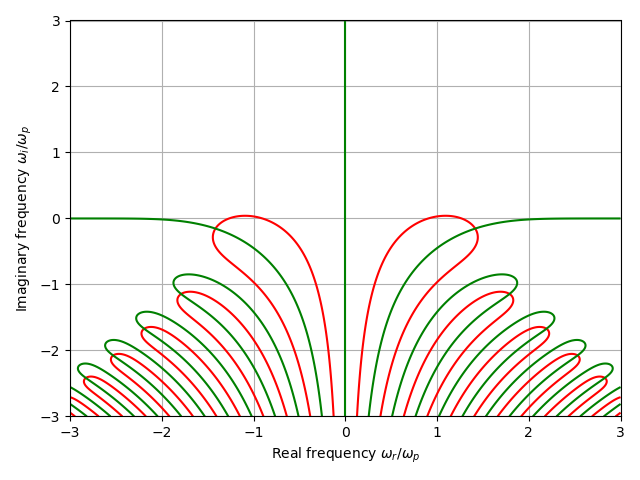
Figure 1: Locations of solutions to $\varepsilon(k,\omega)=0$ showing contours of $\text{Re}(\varepsilon)=0$ in red and $\text{Im}(\varepsilon)=0$ in green for a Maxwellian $f_{0}(v)$ at short wavelength, $k\lambda_{D}=0.5$. Solutions to $\varepsilon(k,\omega)=0$ occur at the intersection of the real and imaginary zero-contours. These damped modes represent the transient Landau spectrum which accompanies any simulation of kinetic instability not initialized with an eigenfunction.

In the theory of continuous dielectrics (Landau and Lifshitz, (1946); Nicholson, (1983)), wave energy density consists of electric field energy density multiplied by the so-called Brillouin factor $\partial_{\omega}(\omega\varepsilon_{r})$. The denominator of Eq. 8 evokes the Brillouin factor because for each root $\omega_{n}=k\zeta_{n}$, we have $\partial_{\omega}(\omega\varepsilon)=\omega_{n}\varepsilon_{\omega}(\omega_{n})$. This energy factor $\varepsilon_{\omega}(k,\zeta_{j})$ is monotonically increasing towards the higher Landau modes. For this reason we speculate that in Landau damping the lowest-energy state is also the least-damped mode, and that the lower-energy states are also of greater amplitude in general perturbations.

2.3 Electrostatic eigenfunctions and transient responses

Equation 8 is the response when the initial data $g^{*}(k,\zeta)$ is an entire function of $\zeta$. However, the phase space linear response Eq. 6 itself has a simple pole. Since the initial data supplied to the kinetic equation is supposed to simulate the self-consistent response of the plasma to some perturbation, it follows that appropriate initial data may also have a pole. Consider the initial condition to be the linear response,

$$g(k,v)=-\frac{q}{m}\frac{1}{k^{2}}\frac{1}{\zeta_{n}-v}\frac{\partial f_{0}}{\partial v}$$ (10)

where $\zeta_{n}$ is a root of the dielectric function, $\varepsilon(k,\zeta_{n})=0$. The Cauchy transform of Eq. 10 is the dielectric function with an added residue for $\text{Im}(\zeta)<0$,

$$g^{*}(k,\zeta)=\frac{\sigma}{\zeta-\zeta_{n}}\Big{(}\varepsilon(k,\zeta)+\begin{cases}0,&\text{Im}(\zeta_{n})>0\\ \frac{2\pi i}{k^{2}}\frac{\partial f_{0}}{\partial v}\Big{|}_{v=\zeta_{n}},&\text{Im}(\zeta_{n})<0\end{cases}\Big{)}$$ (11)

Consider first $\text{Im}(\zeta)>0$. Combining Eqs. 7 and 11 and performing an inverse Fourier transform with Eq. 2 gives the potential $\varphi=k^{-2}e^{i(kx-\omega_{n}t)}.$ The phase space structure is given by Eq. 6, and again observing the form of Eq. 10 and combining with the expression for the potential gives

$$f_{1}(x,v,t)=g(k,v)e^{i(kx-\omega_{n}t)}.$$ (12)

Therefore Eq. 12 is a linear eigenfunction of the Vlasov equation. The phase space fluctuation grows in time and there is no phase mixing. On the other hand, in the case of $\text{Im}(\zeta)<0$ the spectral potential contains a residue,

$$\varphi(k,\zeta)=\frac{i}{k^{3}}\frac{1}{\zeta-\zeta_{n}}-\frac{2\pi}{k^{3}}\frac{1}{(\zeta-\zeta_{n})\varepsilon(k,\zeta)}\frac{1}{k^{2}}\frac{\partial f_{0}}{\partial v}\Big{|}_{v=\zeta_{n}}.$$ (13)

Equation 13 has a double pole at $\zeta=\zeta_{n}$ in the second term, and a simple pole at all other roots $\varepsilon(k,\zeta_{j})=0$ with $j\neq n$. Inverting the solution obtains the expression

$$\begin{split}\varphi(k,t)&=\Big{\{}1+\frac{i\pi}{k^{2}}\frac{\varepsilon_{\omega\omega}(k,\zeta_{n})}{\varepsilon_{\omega}^{2}(k,\zeta_{n})}\frac{\partial f_{0}}{\partial v}\Big{|}_{v=\zeta_{n}}\Big{\}}\frac{e^{-i\omega_{n}t}}{k^{2}}\\ &\quad\quad+\sum_{j\neq n}\Big{(}\frac{1}{(\omega_{n}-\omega_{j})\varepsilon_{\omega}(k,\zeta_{j})}\frac{2\pi}{k^{2}}\frac{\partial f_{0}}{\partial v}\Big{|}_{v=\zeta_{n}}\Big{)}\frac{e^{-i\omega_{j}t}}{k^{2}}.\end{split}$$ (14)

Although the kinetic mode with frequency $\omega_{n}$ is preferentially excited by this perturbation, it is evident that all Landau modes are also necessarily involved. The form of Eq. 14 demonstrates phase mixing and decay at the Landau damping frequencies. However, at long wavelength the mode propagates decoupled from the others to $\mathcal{O}(k^{-2})$.

So far the results are independent of the specific form of $f_{0}(v)$ other than its spatial uniformity. Now, to illustrate the partition of energy into the damped modes, the relative response amplitudes to (a) a Maxwellian perturbation and (b) one with a single pole, namely Eq. 10, are computed for a Maxwellian equilibrium distribution $f_{0}(v)$. In case (a) the Maxwellian perturbation evolves with the potential

$$\varphi(k,t)=-2\sum_{j}\frac{Z(\widetilde{\zeta}_{j})}{Z^{\prime\prime}(\widetilde{\zeta}_{j})}e^{-i\omega_{j}t}$$ (15)

where $\widetilde{\zeta}_{j}=\zeta_{j}/v_{t}$, while case (b) evolves with the potential

$$\varphi(k,t)=\frac{1}{k^{2}}\Big{\{}\Big{(}1-2\pi i\frac{Z^{\prime\prime\prime}(\widetilde{\zeta}_{n})}{(Z^{\prime\prime}(\widetilde{\zeta}_{n}))^{2}}\frac{\partial f_{0}}{\partial v}\Big{)}e^{-i\omega_{n}t}-4\sqrt{2}\pi\frac{\partial f_{0}}{\partial v}\sum_{j\neq n}\frac{e^{-i\omega_{j}t}}{(\zeta_{n}-\zeta_{j})Z^{\prime\prime}(\widetilde{\zeta}_{j})}\Big{\}}.$$ (16)

Figure 2 compares these relative potential amplitudes for the two cases (a) and (b), where (b) represents a rightward-propagating Langmuir wave. While mostly the primary plasma oscillation mode is excited, the higher modes make a substantial contribution.

In summary, Landau damping modes are not eigenfunctions of the Vlasov equation. If they are initialized and time is run either forward or backward they damp through phase mixing in either direction of time. However, their phase space structure is essentially the same as that of the unstable eigenfunctions, namely the plasma part of the plasma-field configuration occurring in a plasma wave. On the other hand, unstable modes are true eigenfunctions whose phase space structures do not change in time.

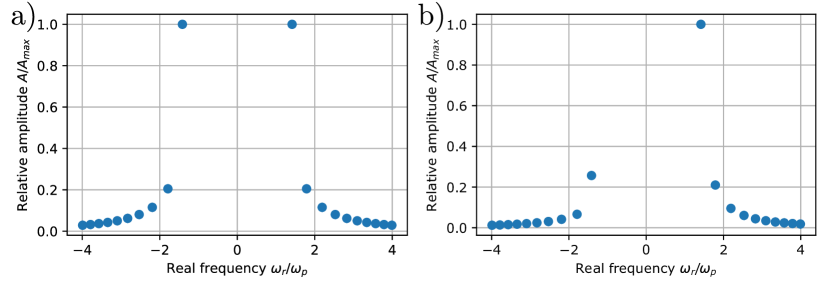
Figure 2: Relative potential amplitudes (normalized to the highest magnitude) of the Landau damping spectrum for the first $\pm 10$ frequencies $\omega_{j}$ given a Maxwellian equilibrium distribution $f_{0}(v)$ at $k\lambda_{D}=0.5$ for a) the Maxwellian perturbation with $g^{*}(\zeta)=Z(\zeta)$, and b) initial data as Eq. 10 with a single complex pole. The modes are ordered by the real part of their frequency. Higher modes are rapidly damped, as seen in Fig. 1 which is computed for the same equilibrium Maxwellian distribution. Case b) shows that while Eq. 10 can excite a propagating, damping plane wave it is necessarily accompanied by transient oscillations in its phase space structure with initial amplitudes up to 20% of the primary oscillation.

2.4 Visualizing the electrostatic phase space eigenfunctions

Let us visually explore the phase space structure just discussed mathematically. Given a solution $\zeta_{n}$ to $\varepsilon(\zeta_{n},k_{n})=0$ for particular $k_{n}$ (for instability, $\text{Im}(k_{n}\zeta_{n})>0$) the perturbed distribution is given by Eq. 12 in complex-conjugate pair. Examining the real part gives

$$f_{1}(x,v,t_{0}) =\alpha\text{Re}(\psi)\frac{\partial f_{0}}{\partial v},$$ (17)

$$\psi(x,v) \equiv\frac{e^{ik_{n}(x-\zeta_{n}t_{0})}}{\zeta_{n}-v}.$$ (18)

Provided that no solution to $\varepsilon(\zeta,k)$ has $\text{Im}(\zeta)=0$ the denominator of $\psi$ does not vanish and the function is well-defined. The complex function $\psi$ is defined for convenience to account for all phase information in the perturbation. The real part is chosen arbitrarily as the linear modes come in conjugate pairs. Note that one can think of the mode as an instantaneous Cauchy transform of the distribution gradient.

For example, consider the two-stream mode of two drifting Maxwellians of drift velocities $v_{d}=\pm 4v_{t}$ with wave-number $k_{0}\lambda_{D}=0.1$, giving a growth rate $\omega_{i}\approx 0.28\omega_{p}$. Figure 3 visualizes the phase space of the corresponding mode given by Eqs. 17-18. The perturbation is a two-dimensional oscillatory structure in phase space, yet the zeroth moment is a pure sine wave resulting in an initial electric potential $\varphi(x)=\varphi_{0}\sin(x)$.

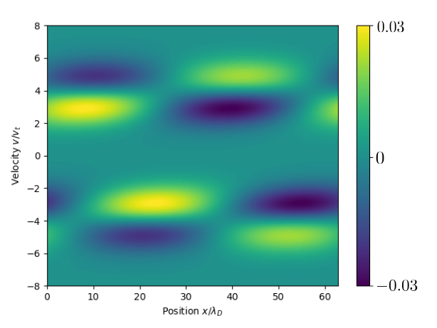
Figure 3: Depicted is the phase space eigenfunction of an unstable two-stream mode on two drifting Maxwellians of drift velocities $v_{d}=\pm 4v_{t}$, which appears as coupled plasma waves on each drifting distribution in the specific sense that the phase space structure on each beam is visually and mathematically similar to a Landau-damped mode of a thermal Maxwellian (i.e. the phase space structure of Eq. 10). However, these plasma wave structures only occur as a normal mode, or eigenfunction, when unstable. The mode has structure in both $x$ and $v$, but its zeroth velocity moment is a pure sine wave and its first moment is zero.

2.5 Phase space eigenfunctions applied to nonlinear initial-value problems

The physically correct initial data is usually discussed in the context of the thermal fluctuation spectrum (Ichimaru, (1992); Yoon, (2007)). Linear eigenfunctions grow from spontaneous thermal fluctuations until nonlinear saturation at some significant fraction of the thermal energy (Crews and Shumlak, (2022)). The Vlasov model does not resolve thermal fluctuations, but this is acceptable for typical plasmas as the magnitude of such fluctuations is much less than the thermal energy.

The eigenfunction part of a general perturbation amplifies its energy while the non-eigenfunction part decays with the same timescale $\omega_{p}^{-1}$. Clearly, with sufficiently small initial amplitude the non-eigenfunction part of a general perturbation does not participate in nonlinear saturation, so that sufficiently low-amplitude general perturbations are physically correct. Yet in the same way, an eigenfunction perturbation of initially large amplitude compared to the thermal fluctuation level is also physically correct. For this reason, eigenfunction perturbations yield a physically meaningful computational cost-savings when initialized with amplitudes just below nonlinear levels, while high-amplitude general perturbations introduce nonlinear Landau damping. Initialization at high amplitude translates to considerable computational savings for high-dimensional, computationally-intesive continuum-kinetic problems.

We mention an application of eigenfunction perturbations to small-amplitude perturbation problems. Sometimes linear instability growth rates are measured for verification of model implementation (Ho et al., (2018); Einkemmer, (2019)). Small-amplitude eigenfunction perturbations allow linear instability growth rates to be deduced from data with basically arbitrary precision because there is a complete absence of Landau damping.

2.5.1 Phase space eigenfunctions applied to the two-stream instability problem

Here we refer to perturbations as “separable” when they factor as $g(x,v)=h(x)f_{0}(v)$ with $h(x)$ representing the desired density perturbation. Given the preceding discussion, it is illustrative to compare energy traces of fully nonlinear Vlasov-Poisson simulations initialized both with general separable perturbations and eigenfunction perturbations. Consider, for example, the two-stream unstable distribution

$$f_{0}(v)=\frac{1}{2\sqrt{2\pi}v_{t}}\Big{(}\exp\Big{\{}-\frac{(v-v_{d})^{2}}{2v_{t}^{2}}\Big{\}}+\exp\Big{\{}-\frac{(v+v_{d})^{2}}{2v_{t}^{2}}\Big{\}}\Big{)}.$$ (19)

Initialization with a separable Maxwellian perturbation, namely $g(x,v)=\alpha f_{0}(v)e^{ikx}$ with $\alpha$ a scalar amplitude, leads to the linear solution

$$\varphi(k,t)=-2\alpha\sum_{j}\frac{Z(\zeta_{+,j})+Z(\zeta_{-,j})}{Z^{\prime\prime}(\zeta_{+,j})+Z^{\prime\prime}(\zeta_{-,j})}e^{-i\omega_{j}t}$$ (20)

where $\zeta_{\pm,j}\equiv(\zeta_{j}\pm v_{d})/\sqrt{2}v_{t}$ are the beam-shifted phase velocities. Table 1 lists the greatest amplitudes of Eq. 20 for drifts $u_{d}=5v_{t}$ at wavenumber $k\lambda_{D}=0.126$, and shows that the unstable mode is only the fifth-largest amplitude. Langmuir waves influence dynamics by masking the growing mode or through nonlinear Landau damping.

Mode	1	2	3	4	5	6
Frequency, $\omega_{r}/\omega_{p}$	$\pm$ 1.42	$\pm$ 0.0157	0	$\pm$ 1.10	$\pm$ 1.20	$\pm$ 1.29
Growth rate, $\gamma/\omega_{p}$	$-3.2\times 10^{-7}$	-0.341	0.335	-0.228	-0.377	-0.488
Amplitude, $|\varphi_{j}|/\text{max}(|\varphi|)$	1	0.710	0.335	0.0701	0.0581	0.0466

Table 1: Relative amplitudes of electric potential for the first six linear mode pairs in a separable perturbation of two counterstreaming thermal plasmas of drift velocities $u_{d}=5v_{t}$ and at wavenumber $k\lambda_{D}=0.126$. In this case, for each non-zero frequency $\omega$ there is a pair of solutions. Due to these mode pairs the unstable mode (here of growth rate $\gamma/\omega_{p}=0.335$) has only the fifth-largest relative amplitude of electric potential in the initial condition (counting the modes twice, as they come in pairs). The significance is that the unstable mode contains only a small fraction of the initialized energy, as all modes occur at the same wavelength. The amplitude and growth rate matching is here only a coincidence.

Figure 4 compares the energy traces of nonlinear simulations of the two-stream instability initialized by both separable and eigenfunction perturbations. When initialized at small amplitude the type of perturbation does not make a difference to saturation dynamics. On the other hand, a perturbation of large amplitude reaches saturation much faster. The large amplitude Maxwellian perturbation in Fig. 4a introduces nonlinearities and changes the energy trace from the desired evolution. Observe that the simulations initialized with the eigenfunction perturbations undergo a pure growth.

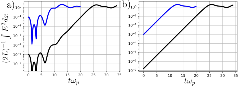
Figure 4: Comparison of energy traces for nonlinear simulations of a single wavelength two-stream instability of drift velocities $u_{d}=5v_{t}$ at wavenumber $k\lambda_{D}=0.126$ showing (a) separable perturbation and (b) eigenfunction perturbation. Two subcases are shown. The black trace represents a small-amplitude perturbation and the blue trace a large-amplitude one. The large-amplitude Maxwellian perturbation introduces nonlinearity, polluting the solution, while the large-amplitude eigenmode saturates equivalently as if seeded from small amplitude. In any case solutions initialized by eigenfunction perturbation undergo pure growth in the linear phase.

2.6 Multidimensional dispersion function for the two-stream instability

Electrostatic turbulence at the Debye length scale generated by streaming instability of electron beams is a ubiquitous plasma phenomenon (Rudakov and Tsytovich, (1978); Che, (2016)), and is inherently three dimensional. This section considers the two-stream instability in the computationally tractable two-dimensional configuration space as an example of the methodology used to compute electrostatic phase space eigenfunctions in multiple dimensions. Recall that the electrostatic dielectric function is determined by

$$\varepsilon(\omega,\bm{k})=1+\frac{\omega_{p}^{2}}{k^{2}}\int\frac{\bm{k}\cdot\nabla_{v}f_{0}}{\omega-\bm{k}\cdot\bm{v}}d\bm{v}=0.$$ (21)

Now consider a thermal two-stream distribution with equal temperatures on each beam,

$$\begin{split}f_{0}(u,v,w)=\frac{e^{-(v^{2}+w^{2})/(2u_{t}^{2})}}{2(2\pi)^{3/2}u_{t}^{3}}\Big{(}\exp\Big{(}-\frac{(u-u_{d})^{2}}{2u_{t}^{2}}\Big{)}+\exp\Big{(}-\frac{(u+u_{d})^{2}}{2u_{t}^{2}}\Big{)}\Big{)},\end{split}$$ (22)

which differs from Eq. 19 in retaining three components of velocity. Having assumed an isotropic thermal velocity $u_{t}$ greatly simplifies analysis; otherwise complications arise due to the elliptical level-sets of $f_{0}$. Let the wavevector lie in the $(x,y)$-plane and consider Eq. 21. The $w$-component integrates out immediately, while the $(x,y)$-directed velocities must be rotated into the frame of the wavevector. Rotating through an angle $\varphi$ to coordinates $(v_{\parallel},v_{\perp})$, the distribution function is $f_{0}(v_{\parallel},v_{\perp})=(f_{+}+f_{-})/2$ with

$$\begin{split}f_{\pm}\equiv\frac{1}{2\pi u_{t}^{2}}\exp\Big{(}-\frac{(v_{\parallel}\mp\cos(\varphi)u_{d})^{2}}{2u_{t}^{2}}\Big{)}\exp\Big{(}-\frac{(v_{\perp}\pm\sin(\varphi)u_{d})^{2}}{2u_{t}^{2}}\Big{)}\end{split}$$ (23)

Evaluating the integral for each drifting component $f_{\pm}$ as $-Z^{\prime}(\zeta_{\pm})/2u_{t}^{2}$ as in Skoutnev et al., (2019) with drift velocity-shifted phase velocity $\zeta_{\pm}\equiv(\zeta\mp\cos\varphi u_{d})/\sqrt{2}u_{t}$ gives

$$\varepsilon(k,\zeta,\varphi)=1-\frac{1}{(k\lambda_{D})^{2}}\frac{Z^{\prime}(\zeta_{+})+Z^{\prime}(\zeta_{-})}{2}=0.$$ (24)

The wavevector having transverse components to the drift axis decreases the effective drift by the cosine of $\varphi$, leading to maximum growth rate of longitudinal waves parallel to the streaming velocity. However, the growth of these transverse-axis components seeds a multi-dimensional turbulence, depending on the configuration space dimensionality.

2.7 Nonlinear simulation of two-stream instability in two spatial dimensions

Although the fastest growing mode of the two-stream problem has a wavevector aligned with the beam axis (in this case, the $x$-axis), eigenmodes with a long-wavelength transverse wavevector component $k_{\perp}\ll k_{\parallel}$ have comparable growth rates to the fastest mode, as illustrated in Fig. 5 computed using the dielectric function obtained in Eq. 24. In this way, streaming instabilities in unmagnetized plasma produce multi-dimensional Langmuir turbulence as long-wavelength transverse components grow along with the longitudinal modes. In practice this is a three-dimensional phenomenon, but for computational tractability this section presents a simulation of the electrostatic streaming instability in phase space with two space dimensions and two velocity dimensions (2D2V).

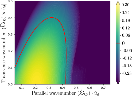
Figure 5: Growth rates of the electron two-stream instability as $\text{Im}(\omega)/\omega_{pe}$ for two counter-streaming Maxwellians with drift speeds relative to the thermal speed of $u_{d}/u_{t}=\pm 3$, in terms of parallel and perpendicular wavenumbers relative to the beam axis vector $\hat{u}_{d}$. The red contour indicates the line of marginal stability where $\text{Im}(\omega)=0$. While the fastest growing mode is aligned with the beam axis (occuring at $(k\lambda_{D})\cdot\hat{u}_{d}\approx 0.2$), modes of comparable growth rates occur with transverse wavelengths roughly five-to-ten times the unstable wavelength on-axis.

2.7.1 Problem set-up and initialization

Our numerical method is summarized in Appendix A. The domain used is periodic and set by fundamental wavenumbers $k_{x}\lambda_{D}=0.05$ and $k_{y}\lambda_{D}=0.02$. The $x$-axis is divided into forty evenly-spaced collocation nodes and the $y$-axis into fifty nodes. Velocity space is truncated at $v_{\max}=\pm 11.5v_{t}$, and each axis divided into fourteen finite elements each of a seventh-order Legendre-Gauss-Lobatto polynomial basis. A non-uniform velocity grid is used; ten elements are linearly clustered between $v\in(-7.5,7.5)v_{t}$ and two elements into $v\in\pm(7.5,11.5)v_{t}$. The drift velocity in Eq. 22 is set to $u_{d}=3v_{t}$. Finally, a spatial hyperviscosity $\nu\nabla_{x}^{4}f$ with $\nu=10$ is added to the kinetic equation to mitigate spectral blocking with this low spatial resolution, as in Crews and Shumlak, (2022). Many modes of comparable growth rates are initialized using the eigenfunction perturbations

$$f_{1}(x,y,u,v)=\frac{\alpha}{k}\text{Re}\Big{(}\frac{k_{x}\partial_{u}f+k_{y}\partial_{v}f}{\omega(k_{x},k_{y})-k_{x}u-k_{y}v}\exp(i(k_{x}x+k_{y}y+\theta))\Big{)}$$ (25)

with $\alpha$ an amplitude scalar, $\omega(k_{x},k_{y})$ solution to the dispersion relation for the mode $(k_{x},k_{y})$, and of random phases $\theta$. A total of thirty-three modes are excited, each with the amplitude $\alpha=0.01$; for each harmonic of the $x$-fundamental $k_{n,x}=nk_{1,x}$ with $n=2$, $3$, and $4$, eleven harmonics of the $y$-fundamental are excited with $k_{m,y}=mk_{1,y}$ with $m=0$, $\pm 1$, $\pm 2$, $\pm 3$, $\pm 4$, and $\pm 5$. There is no symmetry in the $y$-direction as different phases $\theta$ are used for the modes $\pm m$. Mode $n=1$ has small growth rate and is not initialized.

2.7.2 Two-dimensional nonlinear simulations of the streaming instability

The simulation is run to a stop time of $t\omega_{p}=30$. Figure 6 shows the simulation’s electric field energy trace. Hyperviscosity with this spatial resolution leads to a domain energy loss of $\mathcal{O}(10^{-3})$ while electric energy saturates at $\mathcal{O}(10^{-1})$. Due to the use of eigenfunction perturbations there are no oscillations in the electric field energy trace. Therefore, the simulation was initialized with a perturbation energy just two orders below saturation. In this case, this saves approximately $10/\omega_{p}$ of simulation time compared to, for example, a perturbation of initial energy $10^{-6}$.

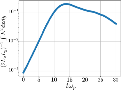
Figure 6: Electric energy trace of the 2D2V two-stream instability with thirty-three excited domain modes. Initialization with eigenmodes enables a perturbation just two decades below saturation energy. The aggressive spatial hyperviscosity of $\nu=10$ leads to an energy loss of $\mathcal{O}(10^{-3})$ by the stop time of this simulation. This artificial dissipation would not be necessary with greater spatial resolution, but the loss is well beneath the electric energy at the stop time.

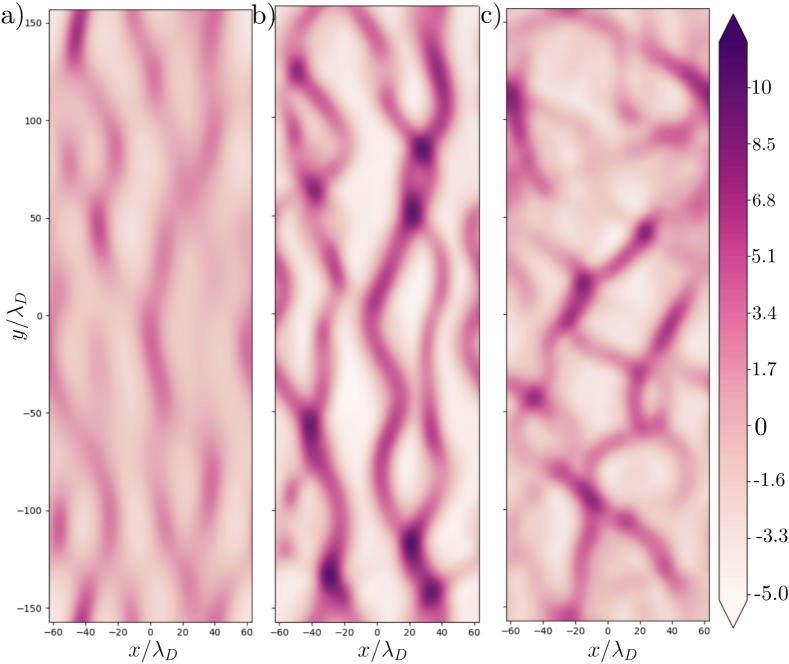
Figure 7: Electric potential $\varphi(x,y)$ of the 2D2V electron two-stream instability for three times: a) $t\omega_{p}=8$ (linear phase); b) $t\omega_{p}=18$ (nonlinear phase); c) $t\omega_{p}=27$ (isotropizing). The evolution begins with the formation of one-dimensional electron holes, or phase space vortex lines, transverse to the streaming axis. These vortex lines then break up after saturation into two-dimensional hole structures with more complex orbits which maintain connection to one another by the Vlasov-dynamical conservation of phase space circulation. The lines of potential in this simulation may be understood as a projection of these phase space vortex tubes.

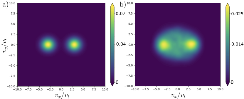
Figure 8: Domain-averaged (coarse-grained) distribution $\langle f\rangle_{(x,y)}(v_{x},v_{y})$ showing relaxation to a Penrose-stable distribution on averaged scales due to multidimensional Langmuir turbulence, for two times: (a) $t\omega_{p}=0$, the unstable initial condition; (b) $t\omega_{p}=30$, the stop time of the simulation. At the end of the simulation the average distribution is double-humped, having heated significantly in the direction transverse to the beam axis compared to the initial state.

Figure 7 plots evolution of electric potential and demonstrates initial predominance of beam-axis wave energy as electron holes form with wavenumber $k_{x}\gg k_{y}$, yet the beam-transverse components with comparable growth rates to the beam-axis components result in two-dimensional structures. The nonlinear phase sees wave energy significantly increase in the beam-transverse direction as the electron holes tilt, consolidate, and isotropize. Figure 8 visualizes evolution of the domain-averaged (coarse-grained) distribution and demonstrates that the consequence of the beam-driven electrostatic turbulence’s isotropization is to distribute energy into the beam-transverse direction. That is, beam-transverse temperature is observed to increase significantly in the resulting marginally stable double-humped distribution (Penrose, (1960)). In effect, heat transfers from coarse-grained wave energy to the coarse-grained distribution (Nicholson, (1983)). These results support the notion that the continuum of electron hole solutions is key to strongly driven plasma transport (Schamel, (2023)).

2.8 Quasilinear kinetic simulation with phase-space eigenfunctions

Quasilinear theory (QLT) is the name given to the simplest closure in the hierarchy of equations resulting from separating the variables of a turbulent system into fluctuating and mean components (Vedenov, (1963); Dodin, (2022)). The scheme of the theory is as follows: a suitable method of averaging is defined, typically temporal, spatial, or ensemble averaging; the dynamical equation is averaged and the mean subtracted from the original equation to obtain the mean and fluctuating components of the system; lastly a closure hypothesis is made by neglecting the “second fluctuation” of the fluctuating equation. Under this procedure the equation for the fluctuation becomes quasilinear and can be solved by spectral methods (Crews and Shumlak, (2022)). As is well known, substitution into the equation for the mean gives a diffusion equation in velocity space.

Diffusion equations are numerically stiff when diffusivity is large. A drawback of QLT posed as a diffusion problem is that the diffusivity is asymptotically singular in the relaxed state of an unstable system. The singularity arises in the theory around the purely real frequencies of the relaxed state (Crews and Shumlak, (2022)). This singularity is side-stepped by solving the equations of QLT as an initial-value problem for a system of first-order equations, resolving both linear eigenfunction growth and Landau damping as a linear phenomenon, and of course the asymptotic ($t\to\infty$) saturation as a quasilinear phenomenon. As a first-order system there is no dimensionality reduction as in the diffusion theory, but significant advantage remains over the fully nonlinear theory as the turbulent nonlinear cascade does not form and only the unstable scales need be resolved. Further, there is no need to solve the dielectric function. To prevent spurious Landau damping it is wise to utilize eigenfunction perturbations, as described in Section 2.5.

To demonstrate we consider the kinetic equation for electrons in a neutralizing background. Splitting the distribution function $f=\langle f\rangle_{L}+\delta f$ where $\langle\cdot\rangle$ is a spatial average, the quasilinear system in normalized units is (Crews and Shumlak, (2022))

$$\frac{\partial\langle f\rangle_{L}}{\partial t} =\frac{\partial}{\partial v}\langle E\delta f\rangle_{L}$$ (26)

$$\frac{d(\delta f)}{dt} =\frac{\partial}{\partial v}(E\langle f\rangle_{L})$$ (27)

with $\frac{d}{dt}=\partial_{t}+v\partial_{x}$ the change along a zero-order trajectory. Consider the expansion of the distribution function in finite Fourier series,

$$f(x,v,t)=f_{0}+\sum_{n=1}^{\infty}\big{(}f_{n}e^{ik_{n}x}+f_{n}^{*}e^{-ik_{n}x}\big{)}.$$ (28)

We identify the DC component of Eq. 28 as the average distribution, $f_{0}=\langle f\rangle_{L}$, and the remaining Fourier coefficients as the Fourier spectrum of the fluctuation. Thus dropping the symbols $\delta(\cdot)$ and $\langle\cdot\rangle_{L}$, Eqs. 26 and 27 are

$$\frac{\partial f_{0}}{\partial t} =\frac{\partial}{\partial v}\langle Ef\rangle_{L},$$ (29)

$$\frac{\partial f_{n}}{\partial t} =-ik_{n}vf_{n}+\frac{\partial}{\partial v}\big{(}E_{n}f_{0}\big{)},$$ (30)

$$E_{n} =ik_{n}^{-1}\int_{-\infty}^{\infty}f_{n}dv,$$ (31)

for $n\neq 0$, where Eq. 31 is obtained from Gauss’s law in the Fourier basis.

2.8.1 Numerical method for the initial-value problem for the quasilinear equations

Equations 29 and 30 are to be discretized in velocity space, and Eq. 31 is applied as a constraint. First, the Fourier series is truncated at a chosen mode number (Galerkin projection) to resolve the range of instability, with the corresponding spatial grid identified as the evenly spaced collocation nodes of the frequency range in a standard manner through the fast Fourier transform. The velocity axis is to be discretized by discontinuous Galerkin method (DG) similarly to the method in Appendix A. We consider the two velocity fluxes in Eqs. 29 and 30,

$$\mathcal{T}(v) =\langle Ef\rangle_{L}=L^{-1}\int_{0}^{L}E\delta f(x,v)dx,$$ (32)

$$\mathcal{M}_{n}(v) =E_{n}f_{0}=\Big{(}ik_{n}^{-1}\int_{-\infty}^{\infty}f_{n}(v^{\prime})dv^{\prime}\Big{)}f_{0}(v).$$ (33)

We evaluate the flux $\mathcal{T}(v)$ by the trapezoidal rule because of its ideal trigonometric quadrature properties (Boyd, (2001)) using the inverse FFT of the spectra $E_{n}$ and $f_{n}(v)$. On the other hand, the fluxes $\mathcal{M}_{n}(v)$ depend only on the local field mode $E_{n}$ and the mean distribution $f_{0}(v)$, so this quantity is simply computed by quadrature in $v$. Both fluxes $\mathcal{T}$ and $\mathcal{M}_{n}$ are then utilized in the DG method as a nonlinear flux. The linear translation operator $ik_{n}vf_{n}$ is discretized by quadrature as in Appendix A, and in the same manner the system is integrated in time semi-implicitly by Strang splitting.

2.8.2 Simulation of the bump-on-tail instability using phase space eigenfunctions

We repeat the calculation of Crews and Shumlak, (2022) for the nonlinear and quasilinear evolutions of the bump-on-tail instability, with the difference that here QLT is solved as an initial-value problem in phase space instead of as a diffusion problem for the reduced distribution. See Crews and Shumlak, (2022) for the details of initialization including the domain and the zero-order distribution. In Crews and Shumlak, (2022) the perturbation is constructed using the phase space eigenfunctions given by Eq. 10. Figure 9 compares the energy traces of the nonlinear and quasilinear simulations where QLT is solved as an initial-value problem, while Fig. 10 compares the spectral phase space at saturation and demonstrates the absence of phase space cascade in QLT. In addition, there is an absence of Landau damping as the perturbation is constructed from eigenfunctions.

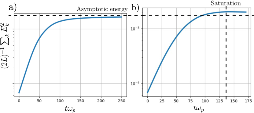
Figure 9: Electric energy traces are compared for (a) the quasilinear evolution, and (b) the fully nonlinear Vlasov-Poisson simulation (from the data of Crews and Shumlak, (2022)) from identical initial conditions and perturbations. The quasilinear system approaches the marginally stable state asymptotically, while the fully nonlinear system saturates in a finite time due to nonlinear particle trapping. Both simulations are initialized at high, yet sub-nonlinear, amplitude without subsequent Landau damping oscillations using phase space eigenfunction perturbations.

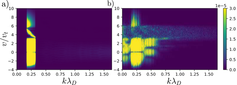
Figure 10: Spectral $(k\lambda_{D},v/v_{t})$ phase space is compared at saturation $t=150\omega_{p}^{-1}$ between (a) the quasilinear system, and (b) the corresponding fully nonlinear Vlasov-Poisson simulation. The spectral phase of the quasilinear system is grossly overresolved in $k\lambda_{D}$ space only for the purpose of comparison; energy remains spatially localized in QLT because the system is unable to cascade through turbulent mixing of phase space eddies, a fully nonlinear phenomenon. The phase space structures in a simulation of QLT remain always as linear eigenfunctions of the form of Eq. 10. In this way sub-Debye length scales need not be resolved in simulation of QLT.

3 Electrostatic eigenmodes with zero-order cyclotron motion

We consider electrostatic phase space eigenfunctions for strongly magnetized plasma by reviewing the linearized theory for the particular case of ring distributions of the so-called Dory-Guest-Harris or $\chi$-distribution type (Dory et al., (1965)), which are of particular interest in space plasmas and magnetic mirror experiments. By strongly magnetized plasma we mean that the zero-order thermal magnetic force $qv_{th}B_{0}$ exceeds the first-order perturbation force $qE_{1}$ such that the zero-order trajectories are taken to be cyclotron motion. Strongly magnetized electrostatic modes are longitudinal oscillations characterized by two fundamental frequencies, the plasma frequency $\omega_{p}$ and the cyclotron frequency $\omega_{c}$. Defining the obliquity through $\hat{\bm{k}}\cdot\bm{B}=kB\cos(\phi)=k_{\parallel}B$, the wavevector decomposes as $\bm{k}=k_{\parallel}\hat{e}_{\parallel}+k_{\perp}\hat{e}_{\perp}$. The spectrum is determined by the roots of the dielectric function $\varepsilon(\omega,k_{\perp},k_{\parallel})=0$, and is strongly dependent on the angle between the wavevector $\bm{k}$ and magnetic field $\bm{B}$. In contrast to the unmagnetized case there are undamped waves perpendicular to $\bm{B}$, including the well-known Bernstein waves of the Maxwellian plasma (Bernstein, (1958)). We will see that the electrostatic phase space eigenfunctions have a helical structure in the perpendicular velocity phase space.

3.1 Review of the Harris dispersion relation

Coordinates are chosen such that $\bm{B}=B\hat{z}$, $\bm{k}=k_{\perp}\hat{x}+k_{\parallel}\hat{z}$ and the velocity space is expressed in cylindrical coordinates as $\bm{v}=v_{\perp}\cos(\phi)\hat{v}_{x}+v_{\perp}\sin(\phi)\hat{v}_{y}+v_{\parallel}\hat{v}_{z}$. In these coordinates the Vlasov equation linearizes around $f_{0}(v_{\perp},v_{\parallel})$ as, with $\omega_{c}=qB/m$,

$$\frac{\partial f_{1}}{\partial t}+v_{\perp}\cos\phi\frac{\partial f_{1}}{\partial x}+v_{\parallel}\frac{\partial f_{1}}{\partial z}-\omega_{c}\frac{\partial f_{1}}{\partial\phi}=\frac{q}{m}\Big{(}E_{x}\cos\phi\frac{\partial f_{0}}{\partial v_{\perp}}+E_{z}\frac{\partial f_{0}}{\partial v_{\parallel}}\Big{)}.$$ (34)

The linearized equation is then Fourier transformed $(x,z,t)\to(k_{\perp},k_{\parallel},\omega)$ to yield

$$\frac{df_{1}}{d\phi}+i\frac{\omega-k_{\perp}v_{\perp}\cos\phi-k_{\parallel}v_{\parallel}}{\omega_{c}}f_{1}=-i\frac{q\varphi}{m}\Big{(}k_{\perp}\cos\phi\frac{\partial f_{0}}{\partial v_{\perp}}+k_{\parallel}\frac{\partial f_{0}}{\partial v_{\parallel}}\Big{)}.$$ (35)

Equation 35 is a first order inhomogeneous equation in the cylindrical velocity-space angle $\phi$ and can be solved by the usual methods. Integrating the inhomogeneous term along the solution of the homogeneous equation yields

$$f_{1}(v_{\perp},\phi,v_{\parallel})=-\frac{q\varphi(k)}{m}\exp(ik_{\perp}v_{y}/\omega_{c})\Big{[}\frac{1}{v_{\perp}}\frac{\partial f_{0}}{\partial v_{\perp}}\Upsilon_{1}+k_{\parallel}\frac{\partial f_{0}}{\partial v_{\parallel}}\Lambda_{1}\Big{]}$$ (36)

where the terms $\Upsilon_{1}$ and $\Lambda_{1}$ are auxiliary wavefunctions defined as the polar Fourier series

$$\Upsilon_{1} =\sum_{n=-\infty}^{\infty}\frac{n\omega_{c}}{\omega-k_{\parallel}v_{\parallel}-n\omega_{c}}J_{n}(k_{\perp}v_{\perp}/\omega_{c})e^{in\phi},$$ (37)

$$\Lambda_{1} =\sum_{n=-\infty}^{\infty}\frac{\omega_{c}}{\omega-k_{\parallel}v_{\parallel}-n\omega_{c}}J_{n}(k_{\perp}v_{\perp}/\omega_{c})e^{in\phi}.$$ (38)

The terms of the series $\Upsilon_{1}$ associated with perpendicular propagation decay one order slower in $n$ than the series $\Lambda_{1}$, meaning that high-order resonances are more important for the perpendicular propagation component. Equation 36 is the phase space linear response for electrostatic fluctuations in a strongly magnetized plasma.

The self-consistent spectrum consists of all pairs $(\omega,k_{\perp},k_{\parallel})$ such that the zeroth moment of $f_{1}(\omega,k_{\perp},k_{\parallel},v_{\perp},\phi,v_{\parallel})$ results in an electric potential mode of wavenumber $(k_{\perp},k_{\parallel})$. Integration of the phase space fluctuation gives the density fluctuation as

$$n_{1}(\omega,k_{\perp},k_{\parallel})=-i\frac{q\varphi}{m}\int_{-\infty}^{\infty}\int_{0}^{\infty}\Big{[}\frac{1}{v_{\perp}}\frac{\partial f_{0}}{\partial v_{\perp}}\Upsilon_{2}+k_{\parallel}\frac{\partial f_{0}}{\partial v_{\parallel}}\Lambda_{2}\Big{]}2\pi v_{\perp}dv_{\perp}dv_{\parallel}$$ (39)

where a set of additional series, analogs of Eqs. 37 and 38, are defined as

$$\Upsilon_{2} =\sum_{n=-\infty}^{\infty}\frac{n\omega_{c}}{\omega-k_{\parallel}v_{\parallel}-n\omega_{c}}J_{n}^{2}(k_{\perp}v_{\perp}/\omega_{c}),$$ (40)

$$\Lambda_{2} =\sum_{n=-\infty}^{\infty}\frac{\omega_{c}}{\omega-k_{\parallel}v_{\parallel}-n\omega_{c}}J_{n}^{2}(k_{\perp}v_{\perp}/\omega_{c}).$$ (41)

Substitution of $n_{1}$ into Poisson’s equation gives Harris’s dispersion relation

$$\varepsilon(\omega,k_{\perp},k_{\parallel})\equiv 1-\Big{(}\frac{\omega_{p}}{\omega_{c}}\Big{)}^{2}\frac{1}{(k\lambda_{D})^{2}}\int_{-\infty}^{\infty}\Big{(}\mathbb{V}_{\perp}f_{\parallel}+k_{\parallel}\mathbb{V}_{\parallel}\frac{\partial f_{\parallel}}{\partial v_{\parallel}}\Big{)}dv_{\parallel}=0$$ (42)

where the integration over perpendicular velocities is broken out into the two quantities

$$\mathbb{V}_{\perp} =\int_{0}^{\infty}\frac{1}{v_{\perp}}\frac{\partial f_{\perp}}{\partial v_{\perp}}\Upsilon_{2}(v_{\perp},v_{\parallel})2\pi v_{\perp}dv_{\perp},$$ (43)

$$\mathbb{V}_{\parallel} =\int_{0}^{\infty}f_{\perp}\Lambda_{2}(v_{\perp},v_{\parallel})2\pi v_{\perp}dv_{\perp},$$ (44)

and separability of the background $f_{0}(v_{\perp},v_{\parallel})=f_{\perp}(v_{\perp})f_{\parallel}(v_{\parallel})$ has been assumed.

3.2 Amplitude limitation of linearization around zero-order cyclotron orbits

Given a zero-order spatially uniform magnetic field $B=\bm{B}_{0}$ and first-order electric field perturbations $\bm{E}=\bm{E}_{1}$, the zero- and first-order kinetic equations are

$$(\bm{v}\times\bm{B}_{0})\cdot\nabla_{v}f_{0} =0,$$ (45)

$$\partial_{t}f_{1}+\bm{v}\cdot\nabla_{x}f_{1}+\frac{q}{m}(\bm{v}\times\bm{B}_{0})\cdot\nabla_{v}f_{1}+\frac{q}{m}\bm{E}_{1}\cdot\nabla_{v}f_{0} =0$$ (46)

assuming a homogeneous zero-order distribution $f_{0}=f_{0}(\bm{v})$. Equation 45 indicates gyrotropy of $f_{0}$ (Gurnett and Bhattacharjee, (2017)). This ordering is valid when the zero-order cyclotron acceleration is much greater than the electrostatic acceleration of a typical particle. Validity translates to an amplitude restriction on electric potential and the density fluctuation. Assuming $k_{\parallel}=0$ and comparing terms proportional to $\nabla_{v}f_{0}$ in Eqs. 45 and 46 for a thermal particle gives $E_{1}\ll v_{th}B_{0}$. Estimating the field $E_{1}$ of wavenumber $k$ by Gauss’s law gives $E_{1}=e\delta n/k\varepsilon_{0}$ for density fluctuation $\delta n$. Combining these estimates results in equivalent conditions on amplitude as measured by $\delta n$ or $\varphi$,

$$\frac{\delta n}{n_{0}} \ll\Big{(}\frac{\omega_{c}}{\omega_{p}}\Big{)}^{2}(kr_{L}),$$ (47)

$$\frac{e\varphi}{kT} \ll\frac{1}{kr_{L}},$$ (48)

for Larmor radius $r_{L}=v_{th}/\omega_{c}$. Amplitudes which exceed these inequalities are subject to electrostatic Landau damping as the dielectric function of Eq. 42 is not valid. Typical cyclotron instabilities have $k_{\perp}r_{L}\approx 1$ which limits the amplitudes of the linear modes considered in this section to amplitudes $\delta n/n_{0}\ll(\omega_{c}/\omega_{p})^{2}$ and $e\varphi\ll kT$.

3.3 The dielectric function for loss cones ($\chi$-distributions)

The linear mode spectrum depends on the background distribution (the zero-order equilibrium). Plasma theory textbooks consider Maxwellian plasmas by expansion in the cyclotron harmonics (Gurnett and Bhattacharjee, (2017)). However, in ideal collisionless plasmas with plasma parameter $\Lambda\to\infty$ distributions are expected to be observed only close enough to Maxwellian such that the Penrose criterion is satisfied.

Recent analytical work on non-Maxwellian distributions focuses on the kappa distributions (Mace and Hellberg, (2009)) to model observations in space plasma (Pierrard and Lazar, (2010)). Kappa distributions, also called q-Gaussians, are motivated by recent advances in entropy methods (Livadiotis and McComas, (2023); Zhdankin, (2023)). It is thought that such entropy methods may facilitate the extension of maximum entropy principles to the prediction of metastable equilibria such as non-Maxwellian velocity distributions or self-organized equilibria in magnetic confinement such as tokamaks (Dyabilin and Razumova, (2015)) and Z pinches (Crews et al., (2024)). Ewart et al., (2022) is a significant recent advance with a lucid description of collisionless relaxation.

Spatially uniform strongly magnetized plasmas must have zero-order gyrotropy so that non-Maxwellian features in perpendicular velocity space are typically ring-shaped. Ring distributions commonly arise from the loss cone mechanism of magnetic traps or planetary magnetospheres. Early identifications of velocity-space instability in ring-distributed plasmas were made by Dory et al., (1965). Dory’s ring distribution, known in the mathematics literature as a $\chi$-distribution, is a type of maximum entropy distribution subject to two constraints on variance.The studies of Tataronis and Crawford, 1970a and Tataronis and Crawford, 1970b extended the theory to oblique propagation, showing maximal growth rates for near-perpendicular propagation, though analytical work was performed only with singular ring distributions. Around the turn of the millennium $q$-analogs of Dory’s analytic ring distributions were introduced by Leubner and Schupfer, (2001) and extended in Pokhotelov et al., (2002), motivated by the successful use of $\kappa$-distributions as $q$-deformations of Maxwell-Boltzmann statistics. Dory’s $\chi$-distribution is the $q\to 1$ limit of Leubner’s $\kappa$-like ring distributions in the same way that the Maxwell-Boltzmann distribution is the $q\to 1$ limit of the $q$-Gaussian (or $\kappa$-) distributions.

For this reason, in this section we focus on Dory’s ring distribution and analyze the dielectric function for such rings assuming separability of the zero-order distribution as

$$f_{0}(v_{\parallel},v_{\perp})=f_{\parallel}(v_{\parallel})f_{\gamma}(v_{\perp})$$ (49)

where $f_{\parallel}(v_{\parallel})$ is a Maxwellian of thermal velocity $v_{t}$ and $f_{\gamma}(v_{\perp})$ is Dory’s ring function

$$f_{\gamma}(v)=\frac{1}{\pi\alpha^{2}}\frac{1}{\Gamma(\gamma+1)}\Big{(}\frac{v^{2}}{\alpha^{2}}\Big{)}^{\gamma}\exp\Big{(}-\frac{v^{2}}{\alpha^{2}}\Big{)}$$ (50)

of thermal velocity $\alpha$ and parameter $\gamma$. The function $f_{\gamma}$ is a two-dimensional distribution,

$$\int_{0}^{\infty}f_{\gamma}(v)2\pi vdv=1,\quad\text{Re}(\gamma)>-1$$ (51)

yet is bounded at zero only for $\gamma\geq 0$. Equation 50 is also known as a $\chi$-distribution and is “two-temperature”. That is, the loss-cone distribution $f_{\gamma}(v_{\perp})$ is the maximum entropy distribution for $v_{\perp}\in[0,\infty)$ subject to the two constraints $\langle v_{\perp}^{2}\rangle=\big{(}\gamma+1\big{)}\alpha^{2}$ and $\big{\langle}(v_{\perp}-\langle v_{\perp}\rangle)^{2}\big{\rangle}=\alpha^{2}\Big{(}1+\gamma-\big{(}\frac{\Gamma(\gamma+3/2)}{\Gamma(\gamma+1)}\big{)}^{2}\Big{)}$ or $\big{\langle}(v_{\perp}-\langle v_{\perp}\rangle)^{2}\big{\rangle}=\frac{1}{4}\alpha^{2}+\mathcal{O}(\gamma^{-1})$ such that the temperature in the gyrating frame is independent of $\gamma$ as $\gamma\to\infty$. Thus the physical meaning of $\alpha$ is the thermal velocity in the gyrating frame, while $\gamma$ is the boost to thermal energy in the laboratory frame (and need not be an integer). In this sense the distribution has two temperatures.

The ring distribution satisfies the recurrence (and $f_{-1}=0$),

$$\frac{1}{v}\frac{df_{\gamma}}{dv}=\frac{1}{\alpha^{2}}\frac{f_{\gamma-1}-f_{\gamma}}{2}.$$ (52)

In the case of ring distributions of the form of Eq. 50, the integrals in both quantities $\mathbb{V}_{\perp}$ and $\mathbb{V}_{\parallel}$ involve only $f_{\gamma}$ due to the recurrence Eq. 52, and suggests defining

$$\mathbb{F}_{n,\gamma}(k)\equiv\int_{0}^{\infty}f_{\gamma}(v)J_{n}^{2}(kv)2\pi vdv$$ (53)

which, as shown in Appendix B, is a type-${}_{2}F_{2}$ hypergeometric function with series representation (Gradshteyn and Ryzhik, (2015))

$$\begin{split}\mathbb{F}_{n,\gamma}(x)=\frac{1}{\Gamma(\gamma+1)}\sum_{\ell=0}^{\infty}&\frac{\Gamma(2n+2\gamma+2\ell+1)}{\Gamma^{2}(n+\ell+1)\Gamma(2n+\ell+1)}\frac{(-1)^{\ell}}{\ell!}x^{2(\ell+n)}.\end{split}$$ (54)

We now proceed with integrating this power series over the parallel velocities. First, we can make a note on an alternative possibility. Rather than integrating the auxiliaries Eqs. 40 and 41 in their summation form, it is possible to first close the summation with the Lerche-Newberger summation theorem (Newberger, (1982)), and to determine the perpendicular velocity integrals in Eqs. 43 and 44 in closed form as hypergeometric functions, as in Appendix C, for arbitrary $k_{\parallel}$. However, the integration over parallel velocities must then proceed by a series expansion around the poles of these hypergeometric functions, making a power series approach inevitable. On the other hand, the power series developed in this section maintains separability of terms containing the parallel velocity.

Proceeding to the integration over parallel velocities, with the parallel distribution $f_{\parallel}(v_{\parallel})$ taken as a Maxwellian distribution, the two integrals are

$$\int_{-\infty}^{\infty}\frac{n\omega_{c}}{\omega-k_{\parallel}v_{\parallel}-n\omega_{c}}f_{\parallel}dv_{\parallel} =-\frac{n}{k_{\parallel}}Z(\zeta_{n})$$ (55)

$$\int_{-\infty}^{\infty}\frac{\omega_{c}}{\omega-k_{\parallel}v_{\parallel}-n\omega_{c}}\frac{\partial f_{\parallel}}{\partial v_{\parallel}}dv_{\parallel} =\frac{1}{2k_{\parallel}}Z^{\prime}(\zeta_{n})$$ (56)

where $Z(\zeta)$ is the plasma dispersion function and the cyclotron harmonic-shifted phase velocity is defined as $\zeta_{n}\equiv\frac{\omega-n\omega_{c}}{\sqrt{2}k_{\parallel}v_{t}}$. Thus the dielectric function for loss-cones is

$$\begin{split}\varepsilon(\omega,k)&=1-\Big{(}\frac{\omega_{p}}{\omega_{c}}\Big{)}^{2}\frac{1}{(kr_{L})^{2}}\sum_{n=-\infty}^{\infty}\Big{[}Z^{\prime}(\zeta_{n})\mathbb{F}_{n,\gamma}(k_{\perp}r_{L})\\ &\quad\quad\quad+\frac{n}{k_{\parallel}r_{L}}Z(\zeta_{n})\Big{\{}\mathbb{F}_{n,\gamma-1}(k_{\perp}r_{L})-\mathbb{F}_{n,\gamma}(k_{\perp}r_{L})\Big{\}}\Big{]}.\end{split}$$ (57)

Equation 57 reduces to the standard series for a Maxwellian ($\gamma=0$) by the identity $\mathbb{F}_{n,0}(k)=e^{-k^{2}}I_{n}(k^{2})$ where $I_{n}(k)$ is the modified Bessel function of the first kind.

3.4 Propagation purely perpendicular to the magnetic field

In the limit of perpendicular propagation, $k_{\parallel}\to 0$, the series Eq. 57 in the cyclotron harmonics simplifies as the terms incorporating proportional to $Z(\zeta_{n})$ vanish. Further, by use of the Lerche-Newberger summation theorem two alternatives to the power series for the perpendicular cyclotron wave dielectric function may be developed which incorporate the contributions from the cyclotron harmonics to all orders. The derivation of these expressions may be found in Appendix C. The first is a closed form, a hypergeometric function with complex poles at the cyclotron resonances,

$$\begin{split}\varepsilon(\omega,k_{\perp})=1+\Big{(}\frac{\omega_{p}}{\omega_{c}}\Big{)}^{2}\frac{1}{(k_{\perp}r_{L})^{2}}\Big{\{}&{}_{2}F_{2}\genfrac{[}{]}{0.0pt}{}{\frac{1}{2},\quad\quad\gamma+1}{1+\omega/\omega_{c},1-\omega/\omega_{c}}(-2(k_{\perp}r_{L})^{2})\\ &-{}_{2}F_{2}\genfrac{[}{]}{0.0pt}{}{\frac{1}{2},\quad\quad\gamma}{1+\omega/\omega_{c},1-\omega/\omega_{c}}(-2(k_{\perp}r_{L})^{2})\Big{\}}=0\end{split}$$ (58)

and the second form is a representation of Eq. 58 as a trigonometric integral generalizing that used in Tataronis and Crawford, 1970a ; Vogman et al., (2014); Datta et al., (2021),

$$\varepsilon(\omega,k)=1+\Big{(}\frac{\omega_{p}}{\omega_{c}}\Big{)}^{2}\csc(\pi\omega/\omega_{c})\int_{0}^{\pi}\sin(\theta)\sin(\theta\omega/\omega_{c})L_{\gamma}(\beta)\exp(-\beta)d\theta$$ (59)

with $\beta\equiv 2\cos^{2}\big{(}\theta/2\big{)}(k_{\perp}r_{L})^{2}$ and $L_{\gamma}(\beta)$ the Laguerre polynomial of order $\gamma$. Hypergeometrics similar to Eq. 58 have been obtained for the Maxwellian plasma and for $\kappa$-distributions (Mace, (2004); Mace and Hellberg, (2009)), and reduce to the Maxwellian result for the parameter $\gamma=0$. Equation 59 is particularly suited to numerical calculation by quadrature. Observe that Eqs. 58 and 59 are naturally functions of frequency and not of phase velocity as there is no ballistic contribution to the zero-order motion. It is hoped that Eqs. 57–59 will be of use in developing analytic forms for the q-analogs to $\chi$-distributions proposed by Leubner and Schupfer, (2001).

3.5 Visualization of the dispersion function and phase space eigenfunctions

Figure 11 plots the electrostatic dispersion function in the complex frequency plane for a loss-cone distribution of $\gamma=6$ for magnetization $\omega_{c}/\omega_{p}=0.1$ at wavenumber $kr_{L}=0.9$. A plethora of solutions to the complex dispersion function $\varepsilon=0$ is illustrated by the intersection of the zeros of the real and imaginary parts, which take place at both solutions and poles. Complex poles at the cyclotron harmonics occur only for the case $k_{\parallel}\to 0$, as evident from the cosecant function $\csc(\pi\omega/\omega_{c})$ in Eq. 59. In this way solutions and simple poles can be clearly distinguished. It is clear that, given zero-order cyclotron orbits, oblique modes are Landau damped but perpendicular modes are not. When wave amplitudes violate the inequality of Eq. 47 nonlinear phenomena occur, and perpendicular waves are also Landau damped. In this situation one may see streaming instabilities in numerical experiments in the magnetization transition regime $\omega_{c}\approx\omega_{p}$.

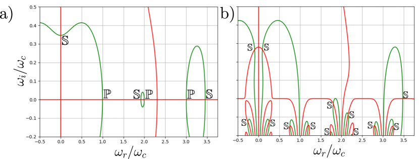
Figure 11: Contours of $\text{Re}(\varepsilon)=0$ (green) and $\text{Im}(\varepsilon)=0$ (red) for the electrostatic dispersion function of a loss cone-distributed plasma with parameters $\omega_{p}=10\omega_{c}$, $\gamma=6$, and $k_{\perp}r_{L}=0.9$ for case a) $90^{\circ}$ propagation and case b) $85^{\circ}$ propagation. Either a solution or a pole occurs at an intersection of these two curve families. Solutions to the dispersion relation $\varepsilon(\omega,k)=0$ are labelled $\mathbb{S}$ while simple poles are labelled $\mathbb{P}$. There are no poles for oblique $(<90^{\circ})$ propagation. Solutions correspond to the first few electron Bernstein modes. The dispersion function shows Gaussian-like responses in the lower-half plane for the oblique wave, an indicator of dissipative wave-particle resonance near the cyclotron harmonics.

Therefore perpendicularly propagating linear modes do not experience Landau resonance so that all such modes are true eigenfunctions. The phase space structure associated with these cyclotron waves (that is, Eq. 36) consists of helical modes in the perpendicular velocity space, since the primary phase component is $\exp(i(kx+n\phi-\omega t))$ for a mode with frequency $\omega\approx n\omega_{c}$, with $\phi$ the cylindrical velocity space angle. The simplest example of such helical phase space modes are the electron Bernstein modes. Figure 12 visualizes the eigenfunctions of the first and second cyclotron harmonics for a Maxwellian background distribution $f_{0}(v_{\perp})$ in the phase space $(x,u,v)$ with $(u,v)$ the perpendicular velocity space and $x$ the propagation coordinate perpendicular to the background magnetic field. With non-zero real frequency these helical modes propagate through phase space.

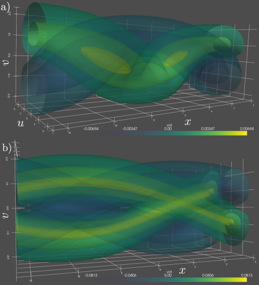
Figure 12: Phase space eigenfunctions of (a) the first and (b) the second cyclotron-harmonic electron Bernstein waves propagating orthogonal to $\bm{B}_{0}$, visualized in the phase space $(x,u,v)$. The order of the cyclotron harmonic determines the number of helical strands of a given sign. The phase space eigenfunction propagates in the lab frame, but when the velocity space is observed at a fixed spatial coordinate the eigenfunction rigidly rotates in the perpendicular velocity space. Balanced counterpropagating modes produce a stationary wave.

3.6 Simulation of perpendicular electron cyclotron loss-cone instability

A useful single-species model problem is the instability of an electron loss cone to perpendicular cyclotron oscillations in a neutralizing background, as studied in Vogman et al., (2014). Normalizing to the Debye length, plasma frequency, and thermal velocity, and the fields by $E_{0}=v_{th}B_{0}$, the Vlasov-Poisson equations are

$$\partial_{t}f+F^{j}\partial_{j}f=0,$$ (60)

$$\frac{d^{2}\varphi}{dx^{2}}=\int_{-\infty}^{\infty}\int_{-\infty}^{\infty}fdudv-1,$$ (61)

$$F=\begin{bmatrix}u,&\frac{d\varphi}{dx}-vB_{\text{ext}},&uB_{\text{ext}}\end{bmatrix}^{T}$$ (62)

with coordinates $(x,u,v)$. The external magnetic field $B_{\text{ext}}$ is set such that the magnetization parameter $\omega_{c}/\omega_{p}=B_{\text{ext}}$ in normalized units. Two single-mode simulations termed $A$ and $B$ are performed for Eqs. 60–62 in the highly unstable over-dense parameter regime $\omega_{p}=10\omega_{c}$ using as eigenvalues two solutions to $\varepsilon(\omega,k)=0$, namely $(k_{A}\lambda_{D},\omega_{A}/\omega_{c})\approx(0.886,0.349i)$ and $(k_{B}\lambda_{D},\omega_{B}/\omega_{c})\approx(1.4,1.182+0.131i)$ found using the integral form of Eq. 59 with fifty point Gauss-Legendre quadrature.

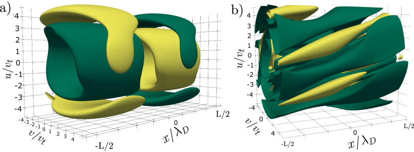
Figure 13: Shown here are the perturbations $f_{1}\equiv f-f_{0}$ at time $t=0$ for a) simulation $A$ with $\omega_{r}=0$ and b) simulation $B$ with $\omega_{r}\neq 0$, each with iso-surfaces at $30\%$ of the minimum (green) and maximum (yellow). The considered eigenfunctions $f_{1}(x,u,v)$ consist of twisting islands in the phase space, capturing the combined physics of translation, electric acceleration, and magnetic gyration. Translating modes ($\omega_{r}\neq 0$) are associated with a helical structure.

In this situation, case $A$ corresponds to a stationary mode with wavelength long compared to the thermal Larmor radius, similar to the two-stream instability studied in the unmagnetized case, while case $B$ corresponds to a destabilized propagating Bernstein-like mode at the first cyclotron harmonic with more significant finite Larmor radius effect. The spatial domain is set to $L=2\pi/k$ in each case and the velocity boundaries to $u_{\text{max}},v_{\text{max}}=\pm 8.5$. We perturb these nonlinear simulations using the phase space eigenfunctions corresponding to the eigenvalue pairs $(k_{A},\omega_{A})$, $(k_{B},\omega_{B})$.

Figure 13 shows isocontours of the phase space eigenfunctions used as the initial perturbations. Case $A$ has a phase space structure similar to the basic plasma wave seen in the two-stream instability, while case $B$ has a helical structure as a cyclotron mode with $\omega_{r}\approx\omega_{c}$. We reiterate here that the eigenfunction perturbation allows arbitrary perturbation amplitude and still produces the same nonlinear phenomena, namely the saturated state or mode coupling/conversion. However, with zero-order $\bm{B}_{0}$ the initial amplitude must not exceed the limit of Eq. 47 or nonlinear phenomena will develop as the perturbation electric force is not first order compared to the thermal magnetic force.

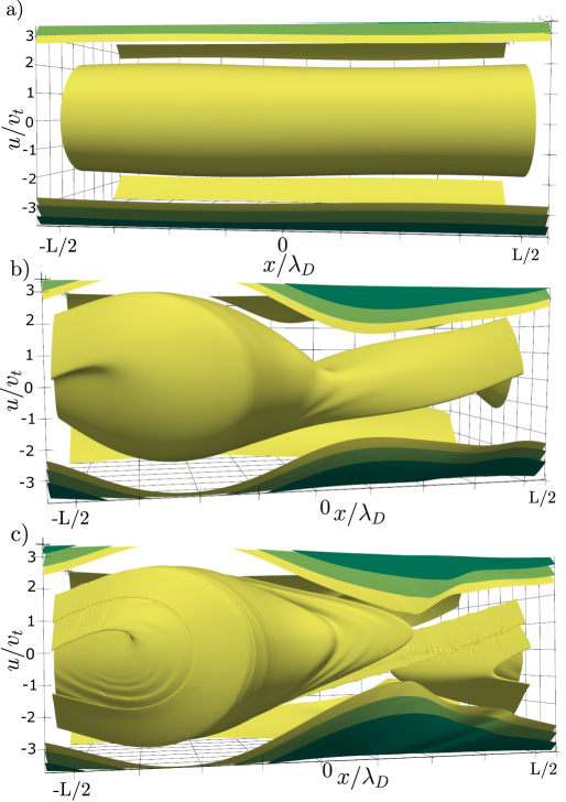
Figure 14: Phase space view $(x,u,v)$ of simulation $A$ focused on $(x,u)$-plane as iso-contours at $15\%$ of $\text{max}(f)$ shown in yellow, at times a) $t=0$, b) $t=80$, and c) $t=120$. The domain within the original ring is shown with $(u,v)\in(-3.5,3.5)$ to focus on the trapping dynamics. The trapping structure consists of a ribbon winding around a separatrix, while the outer bulk ring distribution maintains passing trajectories. This saturation geometry is typical for electrostatic potentials in a magnetic field as the magnetic force depends on the sign of the transverse velocity.

3.6.1 Numerical methods

The problem is evolved numerically using the discontinuous Galerkin (DG) method described in Appendix A and in Crews and Shumlak, (2022), with the difference that the spatial coordinate is not Fourier transformed but also discretized by DG method. We use an element resolution $(N_{x},N_{u},N_{v})=(25,50,50)$ and nodal basis of $n=8$ LGL nodes per dimension, while the Shu-Osher SSPRK3 method is used to integrate the semi-discrete equation in time. These instabilities grow on a slow time-scale relative to the plasma frequency; that is, they grow at a fraction of the cyclotron time-scale $\omega_{c}^{-1}$, while time $t$ is normalized to the plasma frequency $\omega_{p}^{-1}$. Thus these instabilities take many plasma periods to reach nonlinear saturation beginning from amplitudes below the limit of Eq. 47. Simulation $A$ reaches saturation around $t=100$ and runs to $t=175$ while simulation $B$ saturates at around $t=175$ and stops at $t=200$.

Three-dimensional isosurface plots were produced using PyVista, a Python package for VTK. To prepare the data, an average is taken of nodal values lying on element boundaries for smoothness, and the $8$-nodes per element are resampled to $25$ linearly-spaced points per axis and per element onto the basis functions of the DG method. These iso-contours are shown for simulations $A$ and $B$ in Figs. 14 and 15 respectively.

3.6.2 Fully nonlinear single-mode simulation results

Figure 16 shows the electric potentials $\varphi(x)$ in simulations $A$ and $B$. In simulation $A$ the wave potential $\varphi(x)$ is stationary with a weakly fluctuating boundary, so that part of the density $f(x,v)$ within the potential well executes trapped orbits. This results in a trapping structure with orbits tracing a nonlinear potential similar to the characteristic pendulum-like cats-eye separatrix of the single-mode electrostatic two-stream instability. In this case the electrons are magnetized and execute zero-order cyclotron motion so that the trapping separatrix in simulation $A$ is instead in the form shown by the isosurfaces. The saturated state of simulation A is a lattice of one-dimensional strongly magnetized electron holes. The continuum of such hole solutions is key to strongly driven plasma transport physics (Schamel, (2023)). Two-dimensional axisymmetric magnetized holes are the focus of analytical work in Hutchinson, (2020) and Hutchinson, (2021).

The saturated wave potential of simulation $B$, on the other hand, translates with positive phase velocity $\zeta\approx\omega_{r}/k$. The region of particle interaction translates along with the wave potential and forms a vortex structure in the phase space density $f(x,u,v)$. The center of this kink continues to tighten as the simulation progresses, leading to progressively finer structures just as in simulation $A$. This effect is in agreement with the filamentation phenomenon and introduces simulation error as the structures lead to large gradients on the grid scale where discreteness produces dispersion error. For this reason the simulation is stopped at $t=200$. This solution is perhaps somewhat artificial as it is obtained by single-mode initialization via its phase space eigenfunction, thereby not disturbing modes of greater growth rate. This is demonstrated through the energy traces in Fig. 17, showing that simulation $A$ saturates with a greater proportion of the plasma thermal energy than simulation $B$. The solution of simulation B has the significance of a propagating train of nonlinear electrostatic cyclotron waves with associated electron holes, driven unstable by the free energy of a ring distribution.

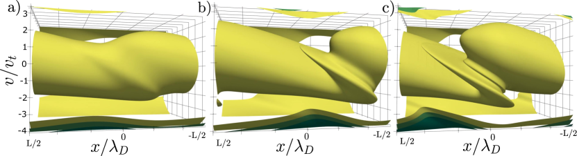
Figure 15: Phase space view looking on $(-x,v)$-plane of simulation B at $15\%$ iso-contours of $\text{max}(f)$ (yellow), with a) the nonlinear mode developing at $t=100$, b) the developed vortex at $t=160$, and c) the saturated vortex translating at $t=180$. The mode is seen to be a growing, translating electrostatic potential $\varphi(x)$ of positive phase velocity $v_{\varphi}=\omega_{r}/k$ with an underlying phase space vortex structure centered at $(u,v)=0$. The vortex shape is explained by considering the trajectory of a test particle in the wave. That is, particles with a velocity close to that of the wave see a stationary potential and are accelerated to a high $u$-velocity. They then translate towards positive $x$ while their velocity vector is rotated by the Lorentz force to $-u$ at a rate close to the wave frequency (as $\omega_{r}\approx 1.2\omega_{c}$) and repeats the cycle.

Figure 16: Electric potentials $\varphi(x)$ at saturation of the two studied cases, for (a) simulation A at $t=120$ and (b) simulation B at $t=180$. The potential of A is stationary while that of B is translating to the right. The negative of potential $-\varphi(x)$ is shown in order to account for the electron’s negative charge. In both cases electron holes develop in the potential wells of $-\varphi(x)$.

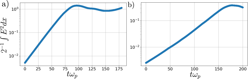
Figure 17: Domain-integrated electric field energy traces for simulations (a) A and (b) B. The thermal energy of the zero-order distribution is $0.25$ per unit length with $\gamma=6$ and $\alpha=1$. In simulation A this corresponds to a domain-integrated thermal energy of $E_{A}\approx 17.8$ and in simulation B to $E_{B}\approx 11.2$. Therefore in both cases the instability saturates with an electric energy a few percent of the thermal energy, approximately $6\%$ in A and $2.5\%$ in B.

3.6.3 Experimental consequences of cyclotron loss-cone instabilities

Magnetic mirror trapping requires the maintenance of a loss-cone distribution in the confined plasma. Simulations such as these, and quasilinear theories, maintain that kinetic instabilities lead to a relaxation of the distribution function on macroscopic scales towards near-Maxwellian distributions, along with long-lived vortical structures in the phase space. By examination of the dispersion functions one finds that phase space instability may be suppressed when $\omega_{p}\ll\omega_{c}$. Assuming equal electron and ion temperatures and densities, we may write for the plasma beta

$$\beta=\Big{(}\frac{v_{ti}}{c}\Big{)}^{2}\Big{(}\frac{\omega_{pi}}{\omega_{ci}}\Big{)}^{2}=\Big{(}\frac{r_{Li}}{\lambda_{i}}\Big{)}^{2}$$ (63)

with $\lambda_{i}=c/\omega_{pi}$ the ion skin depth. Thus, non-Maxwellian features such as ring distributions, as $\chi$-distributions or their $\kappa$-analogs (Pokhotelov et al., (2002); Leubner, (2004)), are expected to persist in very low–$\beta$ plasma, in much the same way in which for weakly magnetized plasma the $\kappa$-distributions persist in the collisionless regime when the plasma parameter $\Lambda\gg 1$. Further discussion on the consequences of mirror instability in high-$\beta$ space plasma can be found in Pokhotelov et al., (2004).

4 Electromagnetic eigenmodes with zero-order ballistic trajectories

We return to weakly magnetized plasma where the zero-order magnetic field is weak compared to perturbations such that zero-order motion is ballistic. We consider the electromagnetic linear response, determine the phase space eigenfunctions and their corresponding electromagnetic eigenfunctions, and utilize them to initialize one- and two-dimensional nonlinear simulations of collisionless electromagnetic instability. We then study the magnetic-trapping electron holes resulting from electromagnetic instability. Purely electromagnetic instability arises from pressure anisotropy, in which case the linear eigenfunctions are known as Weibel instabilities (Weibel, 1959b ), although streaming instability may still be determined as electrostatic theory is contained in the limit $\zeta\ll c$.

Linearization of the Vlasov-Maxwell system around a weakly magnetized spatially uniform equilibrium $f_{0}(\bm{v})$ with no mean drift yields the system

$$\partial_{t}f_{1} +\bm{v}\cdot\nabla_{x}f_{1}+\frac{q}{m}(\bm{E}+\bm{v}\times\bm{B})\cdot\nabla_{v}f_{0}=0,$$ (64)

$$\partial_{t}\bm{B} =-\nabla\times\bm{E},$$ (65)

$$c^{-2}\partial_{t}\bm{E} =-\mu_{0}\bm{j}_{1}+\nabla\times\bm{B}.$$ (66)

Faraday’s equation gives $\bm{B}=\omega^{-1}\bm{k}\times\bm{E}$ such that the spectral Lorentz force is

$$\begin{split}\bm{E}+\bm{v}\times\bm{B}&=\omega^{-1}\big{(}(\omega-\bm{k}\cdot\bm{v})\bm{E}+(\bm{v}\cdot\bm{E})\bm{k}\big{)},\end{split}$$ (67)

and a two-sided-in-time quasi-analysis produces the Vlasov linear response as

$$i\omega f_{1}=\frac{q}{m}\bm{E}\cdot\nabla_{v}f_{0}+\frac{q}{m}(\bm{v}\cdot\bm{E})\frac{\bm{k}\cdot\nabla_{v}f_{0}}{\omega-\bm{k}\cdot\bm{v}}.$$ (68)

The spectral time-derivative of the perturbed current follows as

$$\mu_{0}(-i\omega\bm{j}_{1})=\frac{\omega_{p}^{2}}{c^{2}}\Big{(}\bm{E}-\int\bm{v}(\bm{v}\cdot\bm{E})\frac{\bm{k}\cdot\nabla_{v}f_{0}}{\omega-\bm{k}\cdot\bm{v}}d\bm{v}\Big{)}.$$ (69)

The first term of the phase space linear response has no resonant denominator and thus yields a non-thermal perturbed current independent of the zero-order distribution function, while the second term encodes resonance between the plasma and its wavefield.

4.1 Tensor components for arbitrary Cartesian coordinates

In Cartesian coordinates $(x,y,z)$ with wavevector $\bm{k}=k_{x}\hat{x}+k_{y}\hat{y}+k_{z}\hat{z}$, the dielectric tensor (Skoutnev et al., (2019)) is obtained from combination of Eqs. 69 and 66 as

$$\begin{split}\varepsilon_{ij}E_{j}&=0,\\ \varepsilon_{ij}&=\delta_{ij}-\frac{c^{2}k^{2}}{\omega^{2}}\Big{(}\delta_{ij}-\frac{k_{i}k_{j}}{k^{2}}\Big{)}-\frac{\omega_{p}^{2}}{\omega^{2}}\Big{(}\delta_{ij}-\int v_{i}v_{j}\frac{\bm{k}\cdot\nabla_{v}f_{0}}{\omega-\bm{k}\cdot\bm{v}}d\bm{v}\Big{)}.\end{split}$$ (70)

In the formal initial-value problem an initial-value vector results in the system $\varepsilon_{ij}E_{j}=g_{i}$. Typically in Cartesian form the moment integrals are inseparable because of the resonant denominator $\omega-\bm{k}\cdot\bm{v}$, yet are separable when the frame is chosen with one coordinate aligned with the wave-vector such that the resonant denominator appears as $\omega-kv_{\parallel}$.

4.2 Electromagnetic susceptibility and the eigenvalue problem

Reformulation of Eq. 70 as an eigenvalue problem for the phase velocity $\zeta$ allows calculation of electric field eigenfunctions $\bm{E}$ naturally consistent with the corresponding phase space eigenfunction $f_{1}$ given by Eq. 68. This facilitates construction of initial conditions for simulation of Vlasov-Maxwell instabilities. Multiply by $\omega^{2}$ and pull out the diagonal tensor $\omega^{2}\delta_{ij}$. Define the integrals encoding resonant wave-particle interaction into the self-consistent perturbation current as

$$I_{ij}\equiv\int_{\mathcal{C}}v_{i}v_{j}\frac{\bm{k}\cdot\nabla_{v}f_{0}}{\omega-\bm{k}\cdot\bm{v}}d\bm{v}$$ (71)

where the integral is evaluated on the Landau contour $\mathcal{C}$, i.e. analytically continued to the lower-half complex $\omega$-plane. The dielectric tensor system may then be rewritten as

$$\Big{\{}\delta_{ij}-I_{ij}+(k\lambda_{c})^{2}\Big{(}\delta_{ij}-\frac{k_{i}k_{j}}{k^{2}}\Big{)}\Big{\}}E_{j}=\Big{(}\frac{\omega}{\omega_{p}}\Big{)}^{2}E_{i}$$ (72)

where $\lambda_{c}=c/\omega_{p}$ is the inertial length. The resonant integrals are naturally functions of the phase velocity $\zeta=\omega/k$, so one can also express the system as

$$\frac{1}{(k\lambda_{D})^{2}}\Big{\{}\delta_{ij}-I_{ij}+(k\lambda_{c})^{2}\Big{(}\delta_{ij}-\frac{k_{i}k_{j}}{k^{2}}\Big{)}\Big{\}}E_{j}=\Big{(}\frac{\zeta}{v_{t}}\Big{)}^{2}E_{i}.$$ (73)

Equation 73 casts the problem in eigenvalue form as the system of integral equations

$$\chi(k,\zeta)\vec{E}=\zeta^{2}\vec{E}.$$ (74)

As in the scalar Poisson problem there is a spectrum of solutions $\zeta$ for a given $k$, obtained by determining a root of the characteristic function $D(k,\zeta)\equiv$ det$(\chi-\zeta^{2}I)=0$. As in the scalar problem only unstable solutions satisfying $\text{Im}(\zeta)>0$ constitute normal modes of oscillation. In unmagnetized spatially uniform plasma these modes are either streaming instability (two-stream, Buneman, ion-acoustic) or generalized Weibel instability. In either case their effect is thermalization on averaged scales by reducing relative velocities far from equilibrium. Casting the dispersion tensor for plasma with zero-order cyclotron orbits (Stix, (1992)) into eigenvalue form proceeds in exactly the same manner; the main difference is that the integral functions $I_{ij}$ are sums over resonances at Doppler-shifted cyclotron harmonics and their calculation, though methodical, is lengthy.

Having determined a particular eigenvalue $\zeta_{n}$ such that $D(k,\zeta_{n})=0$, the corresponding electric field eigenfunction $\bm{E}_{n}$ is found by solving for the eigenvector of the matrix $\chi_{n}=\chi(\zeta_{n},k)$ with eigenvalue $\zeta_{n}^{2}$. The other two eigenvalues of the matrix $\chi_{n}$ are spurious as they do not correspond to solutions of Eq. 74. The magnetic field eigenfunction is obtained through $\vec{B}_{n}=\zeta_{n}^{-1}\hat{k}\times\vec{E}_{n}$, and the phase space eigenfunction $f_{1,n}$ from Eq. 68.

4.3 Dielectric tensor components for the anisotropic Maxwellian

In order to illustrate the Weibel instability due to anisotropy in a plasma with zero-order ballistic trajectories it is useful to consider the anisotropic Maxwellian, or multiple-temperature, zero-order distribution (Davidson et al., (1972)). Let $(x,y,z)$ and $(u,v,w)$ be Cartesian coordinates in configuration space and velocity space respectively. Consider a three-temperature Maxwellian distribution given by

$$f_{0}=\frac{1}{(2\pi)^{3/2}\theta_{u}\theta_{v}\theta_{w}}\exp\Big{\{}-\frac{1}{2}\Big{(}\frac{u^{2}}{\theta_{u}^{2}}+\frac{v^{2}}{\theta_{v}^{2}}+\frac{w^{2}}{\theta_{w}^{2}}\Big{)}\Big{\}}.$$ (75)

Anisotropy plays a key role in magnetized plasmas (Mahajan and Hazeltine, (2000)), and the anisotropic Maxwellian is the simplest such model to illustrate Weibel instability. For purpose of illustration we obtain from Eq. 75 one- and two-dimensional model problems of Weibel instability by letting the wavevector lie in the $(x,y)$-plane and the $\hat{z}$-direction to be the wave binormal. These model problems have the advantage of zero-order electrostatic stability such that all eigenfunctions are fully electromagnetic.

With wavevector in the $(x,y)$-plane the off-diagonal integrals $I_{13}$, $I_{23}$ vanish as $\langle w\rangle=0$, so that the $\hat{z}$-directed perturbation does not contribute the $(x,y)$-plane’s perturbation current, decoupling the binormal from the longitudinal and transverse components (Sharma and Bhatnagar, (1976); Datta et al., (2021)). A fully general wavevector would couple all three components of the perturbation. Equation 70 simplifies to

$$\begin{Bmatrix}\omega^{2}-\omega_{p}^{2}(1-I_{11})&\omega_{p}^{2}I_{12}&0\\ \omega_{p}^{2}I_{12}&\omega^{2}-c^{2}k^{2}-\omega_{p}^{2}(1-I_{22})&0\\ 0&0&\omega^{2}-c^{2}k^{2}-\omega_{p}^{2}(1-I_{33})\end{Bmatrix}\begin{Bmatrix}E_{1}\\ E_{2}\\ E_{3}\end{Bmatrix}=0.$$ (76)

Focusing on the $(x,y)$-plane we consider a reduced distribution, the bi-Maxwellian $f_{0}(u,v)=\int f_{0}(u,v,w)dw$ whose level sets form ellipses in the $(u,v)$ velocity plane. Take $\theta_{v}>\theta_{u}$ so that the semi-major axis of each ellipse is $v$-directed and the characteristic eccentricity is $e^{2}=1-\theta_{u}^{2}/\theta_{v}^{2}$. To ensure separability of the resonant integrals $I_{ij}$, the $(x,y)$-plane is rotated through an angle $\varphi$, transforming velocities $(u,v)\to(v_{\parallel},v_{\perp})$ such that the resonant denominator is $\omega-kv_{\parallel}$. By completing the square on $v_{\perp}$, the anisotropic Maxwellian of Eq. 75 in the reduced coordinates $(u,v)\to(v_{\parallel},v_{\perp})$ is

$$f_{0}(v_{\parallel},v_{\perp})=\frac{1}{2\pi\theta_{\parallel}\theta_{\perp}}\exp\Big{(}-\frac{v_{\parallel}^{2}}{2\theta_{\parallel}^{2}}\Big{)}\exp\Big{(}-\frac{(v_{\perp}-\alpha v_{\parallel})^{2}}{2\theta_{\perp}^{2}}\Big{)},$$ (77)

where the rotated thermal and mean velocities are defined as

$$\theta_{\parallel}^{2}\equiv\frac{(1-e^{2})\theta_{u}^{2}}{1-e^{2}\cos^{2}(\varphi)},\quad\theta_{\perp}^{2}\equiv\frac{\theta_{u}^{2}}{1-e^{2}\cos^{2}(\varphi)},\quad\alpha\equiv\frac{e^{2}\sin(\varphi)\cos(\varphi)}{1-e^{2}\cos^{2}(\varphi)}.$$ (78)

Equation 77 shows that the distribution in the rotated frame is Maxwellian in the longitudinal and transverse directions, yet in the frame of reference of a resonant particle of velocity $v_{\parallel}$ the distribution function has a mean velocity $\alpha v_{\parallel}$ transverse to the wavevector, as illustrated in Fig. 18. The off-diagonal integrals are non-zero, $I_{ij}\neq 0$, for anisotropic distributions as the apparent transverse current in the resonant particle frame couples the longitudinal and transverse wave components for propagation not aligned with the principal axes, even though there is no net current in the lab frame. However, the other transverse component, the binormal, is independent. This phenomenon does not occur for isotropic distributions, for which the longitudinal plasma wave and the two components of the transverse electromagnetic wave have fully independent dispersion relations. In general all three components can couple for non-principal propagation.

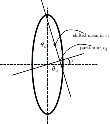
Figure 18: In the frame of reference of a particle propagating in a direction not aligned with the principal axes of an anisotropic distribution there is a mean drift velocity in the direction transverse to the particle’s motion which couples together the electromagnetic wave’s longitudinal and transverse components. In other words, in a frame where the velocity coordinates $(u,v)$ are rotated through an angle $\varphi$ into coordinates $(v_{\parallel},v_{\perp})$, for a particular value of $v_{\parallel}$ there is a non-zero mean value of $v_{\perp}$ such that the off-diagonal integrals $I_{ij}\neq 0$ of Eq. 71.

To evaluate the integrals $I_{11}$, $I_{12}$, and $I_{22}$ for the distribution in Eq. 77 in the rotated coordinates, note the following integrals related to the plasma dispersion function $Z(\zeta)$,

$$\frac{1}{\sqrt{\pi}}\int_{-\infty}^{\infty}\frac{x}{\zeta-x}e^{-x^{2}/2a^{2}}dx =\frac{a}{2}Z^{\prime}(\widetilde{\zeta}),$$ (79)

$$\frac{1}{\sqrt{\pi}}\int_{-\infty}^{\infty}\frac{x^{2}}{\zeta-x}e^{-x^{2}/2a^{2}}dx =-\frac{a^{2}}{2}(Z^{\prime\prime}(\widetilde{\zeta})+2Z(\widetilde{\zeta})),$$ (80)

$$\frac{1}{\sqrt{\pi}}\int_{-\infty}^{\infty}\frac{x^{3}}{\zeta-x}e^{-x^{2}/2a^{2}}dx =\frac{a^{3}}{2^{3/2}}(Z^{\prime\prime\prime}(\widetilde{\zeta})+6Z^{\prime}(\widetilde{\zeta})),$$ (81)

where $\widetilde{\zeta}=\zeta/\sqrt{2}a$. These identities are found through integration by parts using the Hermite relation $\psi_{n}(x)=\frac{d^{n}}{dx^{n}}e^{-x^{2}/2}$ and the identity $Z^{\prime}(\zeta)=-2(1+\zeta Z(\zeta))$. With the gradient $\frac{\partial f}{\partial v_{\parallel}}=\big{(}-v_{\parallel}/\theta_{\parallel}^{2}+\alpha(v_{\perp}-\alpha v_{\parallel})/\theta_{\perp}^{2}\big{)}f$ the integrals $I_{ij}$ in Eq. 76 work out to

$$I_{11} =-\frac{1}{4}(Z^{\prime\prime\prime}(\widetilde{\zeta})+6Z^{\prime}(\widetilde{\zeta})),$$ (82)

$$I_{12} =-\frac{\alpha}{4}(Z^{\prime\prime\prime}(\widetilde{\zeta})+6Z^{\prime}(\widetilde{\zeta})),$$ (83)

$$I_{22} =-\frac{\alpha^{2}}{4}(Z^{\prime\prime\prime}(\widetilde{\zeta})+2Z^{\prime}(\widetilde{\zeta}))-\frac{\theta_{\perp}^{2}}{\theta_{\parallel}^{2}}\frac{Z^{\prime}(\widetilde{\zeta})}{2},$$ (84)

$$I_{33} =-\frac{\theta_{w}^{2}}{\theta_{\parallel}^{2}}\frac{Z^{\prime}(\widetilde{\zeta})}{2},$$ (85)

where $\widetilde{\zeta}\equiv\zeta/\sqrt{2}\theta_{\parallel}$. Let the angular eccentricity be $\gamma=\arcsin(e)$. The characteristic anisotropies are then $A_{1}\equiv\theta_{\perp}^{2}/\theta_{\parallel}^{2}-1=\frac{e^{2}}{1-e^{2}}=\tan^{2}(\gamma)$ for the in-plane anisotropy and $A_{2}\equiv\theta_{w}^{2}/\theta_{\parallel}^{2}-1$ for the binormal anisotropy. These two anisotropy parameters induce electromagnetic Weibel instability to relax the anisotropy of their respective dimensions. For propagation along the principal axes, $\varphi\to 0,\pi/2$ the parameter $\alpha\to 0$, decoupling the $\hat{x}$- and $\hat{y}$-components as $I_{12}\to 0$ and $I_{22}\to-\frac{\theta_{v}^{2}}{\theta_{u}^{2}}\frac{Z^{\prime}(\zeta/\sqrt{2}\theta_{u})}{2}$ as in Eq. 85.

4.3.1 Dispersion function for the classic Weibel instability

Focusing on the decoupled component in Eq. 76, namely $\varepsilon_{33}E_{3}=0$, leads to

$$1-\Big{(}\frac{\zeta}{c}\Big{)}^{2}+\frac{1}{(k\lambda_{c})^{2}}\Big{(}1+\frac{Z^{\prime}(\widetilde{\zeta})}{2}+A_{2}\frac{Z^{\prime}(\widetilde{\zeta})}{2}\Big{)}=0$$ (86)

where $A_{2}\equiv\theta_{w}^{2}/\theta_{\parallel}^{2}-1$ is the anisotropy. For propagation with $\varphi=0$ (that is, in the $\hat{x}$-direction) the anisotropy $A_{1}=\theta_{v}^{2}/\theta_{u}^{2}-1$ and $A_{2}=\theta_{w}^{2}/\theta_{u}^{2}-1$ such that Eq. 86 describes both the transverse and binormal component. Isotropy reduces Eq. 86 to the dispersion relation for an ordinary wave,

$$1-\Big{(}\frac{\zeta}{c}\Big{)}^{2}+\frac{1}{(k\lambda_{c})^{2}}\Big{(}1+\frac{Z^{\prime}(\widetilde{\zeta})}{2}\Big{)}=0.$$ (87)

Equation 76 is also solved by the longitudinal and transverse coupled branch

$$\Big{(}-\Big{(}\frac{\zeta}{c}\Big{)}^{2}+\frac{1}{(k\lambda_{c})^{2}}(1-I_{11})\Big{)}\Big{(}1-\Big{(}\frac{\zeta}{c}\Big{)}^{2}+\frac{1}{(k\lambda_{c})^{2}}(1-I_{22})\Big{)}-\frac{1}{(k\lambda_{c})^{4}}I_{12}^{2}=0$$ (88)

with transverse magnetic field out-of-plane and two components of electric field in-plane.

4.4 Single-mode saturation of Weibel instability in one spatial dimension

Just as electrostatic instability saturates by electrostatic trapping of near-resonant particles in the wavefield, magnetic trapping is the means by which electromagnetic instability saturates. Simulation of a single unstable Weibel eigenfunction allows one to visualize the nonlinear phase space structure of magnetic trapping. Continuum-kinetic simulation of single-mode Weibel saturation was done in Cagas et al., (2017) using as zero-order distribution a pair of counter-streaming electron beams, where electrostatic streaming instability was proposed to explain the growth of beam-axis directed electric field close to nonlinear saturation.

Zero-order beam distributions are often used because Weibel instability is induced in the laboratory by colliding high velocity plasmas (Hill et al., (2005); Fox et al., (2013); Huntington et al., (2015); Shukla et al., (2018)). While zero-order beam distributions are inherently anisotropic they are also possibly unstable to electrostatic streaming instability. The possible introduction of electrostatic streaming instability can confuse and complicate an attempt to isolate Weibel instability. On the other hand, there is no possibility of streaming instability when the Weibel instability is induced by a zero-order anisotropic Maxwellian distribution. In fact, the foundational work on electromagnetic instability of anisotropic distributions analyzed anisotropic Maxwellians by the particle-in-cell method (Davidson et al., (1972)). For this reason the anisotropic Maxwellian is considered here using the continuum kinetic method.

4.4.1 Numerical method

We use the mixed spectral-DG method presented in Appendix A and Crews and Shumlak, (2022), where the space coordinate is represented using Fourier modes and the two velocity dimensions are discretized with discontinuous Galerkin method. The field equations are chosen as follows: Ampere’s law and Faraday’s law are used to evolve the transverse electrodynamic field, and Gauss’s law is used to constrain the electric field along the axis of the wavevector. When considering only a single spatial coordinate three field equations can be chosen in this way (one component each of the electrodynamic equations and Gauss’s law).

The geometry is established by aligning the hot direction of the bi-Maxwellian with the $y$-coordinate, the growing magnetic field with the $z$-direction, and perturbing the distribution function with wavenumber in the $x$-direction. This necessitates two dimensions of velocity, $v_{x}$ in the $x$-direction and $v_{y}$ in the $y$-direction, for a 1D2V phase space geometry. Phase space is discretized using $N_{x}=100$ evenly-spaced collocation nodes in the $x$-direction, and $N_{v_{x}}=N_{v_{y}}=22$ finite elements in velocity, each of $11$th polynomial order. Fourteen elements are evenly spaced between the velocity intervals $[-7,7]v_{t}$, and four elements are evenly spaced within each interval $[-15,-7]v_{t}$ and $[7,15]v_{t}$. A spatial hyperviscosity $10^{-4}\nabla_{x}^{4}f$ is used to prevent spectral blocking by the turbulent cascade saturation. The field equations are discretized by a standard Fourier spectral method.

4.4.2 Initialization with phase space eigenfunctions

The characteristic parameters are chosen such that $v_{t}/c=0.3$ and anisotropy $A=3$ (or ratio $\theta_{v}/\theta_{u}=2$) with the zero-order distribution given by Eq. 75 and the direction of propagation set to $\varphi=0$. This is equivalent to using Eq. 86 for the dispersion function. Velocities are normalized to $\theta_{u}$, time to $\omega_{p}^{-1}$, and lengths to $\lambda_{D}=\theta_{u}/\omega_{p}$. The domain length is then specified by the chosen wavenumber $k_{x}\lambda_{D}=0.1$. Solution of Eq. 86 gives the eigenvalue of the problem as the phase velocity $\zeta/v_{t}=1.23i$. The phase space perturbation is constructed using Eq. 68 for the phase space eigenfunction in the form

$$f_{1}(x,v_{x},v_{y})=\text{Re}\Big{\{}i\frac{\mathcal{A}}{k}\Big{(}\frac{v_{y}}{\zeta-v_{x}}\frac{\partial f_{0}}{\partial v_{x}}+\frac{\partial f_{0}}{\partial v_{y}}\Big{)}\exp(ikx)\Big{\}},$$ (89)

and the initial transverse electrodynamic fields by

$$B_{z1} =\text{Re}\Big{(}\mathcal{A}\exp(ikx)\Big{)},$$ (90)

$$E_{y1} =\text{Re}\Big{(}\zeta\mathcal{A}\exp(ikx)\Big{)},$$ (91)

where the amplitude is set to $\mathcal{A}=10^{-3}$. This initial condition is consistent in the sense that the charge density is zero and the current density satisfies Ampere’s law.

4.4.3 Fully nonlinear simulation results for single-mode Weibel saturation

The simulation is run until $t\omega_{p}=100$ using the time integration method of Appendix A with time-step $\Delta t=2.0\times 10^{-3}$. The change in domain-integrated wave energies is shown in Fig. 19. Of note is that the transverse electric field is oscillatory at saturation, and that the longitudinal electric energy trend generally follows that of the magnetic energy.

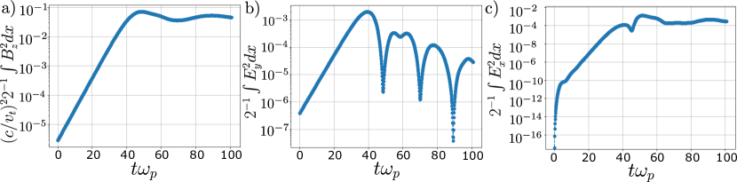
Figure 19: Growth of domain-integrated wave energies towards saturation of Weibel instability in one spatial dimension, namely (a) the magnetic energy, (b) the transverse electric energy of $E_{y}$, and (c) the longitudinal electric energy of $E_{x}$, or energy along the axis of the wavevector. A nonlinear phase is reached at $t\omega_{p}=40$, with peak magnetic energy around $t\omega_{p}=50$. Longitudinal electric energy is observed to grow with a similar trend to the magnetic energy.

Figure 20 shows the time evolution of magnetic field and electron density in increments of $t\omega_{p}=20$. As the magnetic energy grows electrons are progressively trapped by the velocity-dependent force $v_{y}B_{z}$. The magnetic trapping mechanism of nonlinear saturation occurs due to near-resonant particle trapping within the effective potential wells of the electromagnetic field as the distribution function evolves towards a function of the constants of motion, namely the energy $E=\frac{1}{2}m(v_{x}^{2}+v_{y}^{2})-e\varphi(x)$ and components of canonical momentum $p_{y}=mv_{y}-eA_{y}(x)$, $p_{x}=mv_{x}$. Specifically, trapped and passing phase space trajectories are determined by the equation (Morse and Nielson, (1971))

$$mv_{x}=\sqrt{2m(E+e\varphi(x))-(p_{y}+eA_{y}(x))^{2}}$$ (92)

for the particle’s initial energy $E=\frac{1}{2}m(v_{x0}^{2}+v_{y0}^{2})$ and momentum $p_{y}=mv_{y0}$. Figure 21 visualizes magnetic trapping in phase space, showing a contour of the distribution function at $10\%$ of the maximum value. Trapped and passing trajectories are seen at the right and left of the figure, respectively, for $v_{y}>0$. Trapped trajectories circulate within the phase space vortex while passing trajectories execute motion in the vicinity of the separatrix (that is, the vortex’s outer limit). Upon inversion of the transverse velocity, $v_{y}\to-v_{y}$, the positions of the trapped trajectories and passing trajectories are inverted, $x\to-x$, as the sign of the effective potential changes with that of $B_{z}(x)$.

Linear electrostatic instability is not possible due to the zero-order anisotropic Maxwellian, so here we explain the growth of electrostatic energy observed both here and in Cagas et al., (2017) to be a second-order phenomenon arising from space-charge-generating filamentation (that is, the magnetic-trapping electron holes of Fig. 20). While saturated filaments can be understood intuitively as electron holes, the progressive development of longitudinal electric energy in the linear phase should be understood as mode coupling of the longitudinal field to the transverse field at second order in the transverse dynamic field (Taggart et al., (1972)).

Both electric and magnetic field trapping is associated with local variations in the electron density which manifests as space charge. Since the fraction of trapped electrons is proportional to the magnetic energy, with saturation when the characteristic magnetic bounce frequency reaches the growth rate (Davidson et al., (1972)), it follows intuitively that longitudinal electric field should trend nonlinearly with the magnetic field. The Weibel instability’s phase space eigenfunction produces no density fluctuation, so the growth of longitudinal electric field is a nonlinear phenomenon even when the phase space eigenfunction is the principal phase space structure. The development of space charge from magnetic pressure is anticipated in the numerics of Morse and Nielson, (1971), and the longitudinal field is explained in Taggart et al., (1972) to arise at second-order from the coupling of two magnetic modes. Since the magnetic field, plotted in Fig. 20, is observed to evolve into a multi-mode nonlinear wave with the spectral signature of an elliptic cosine, mode pairs are indeed available to couple into the longitudinal field. Dynamic space charge, or filamentation, has been observed in modeling to modify growth rates, in both early and more recent studies (Taggart et al., (1972); Tzoufras et al., (2006)), pointing to the importance of higher-order effects prior to saturation. While the charge density is a second-order effect, the first-order effect of electrodynamic instability is the generation of electric currents to sustain the steadily growing magnetic mode.

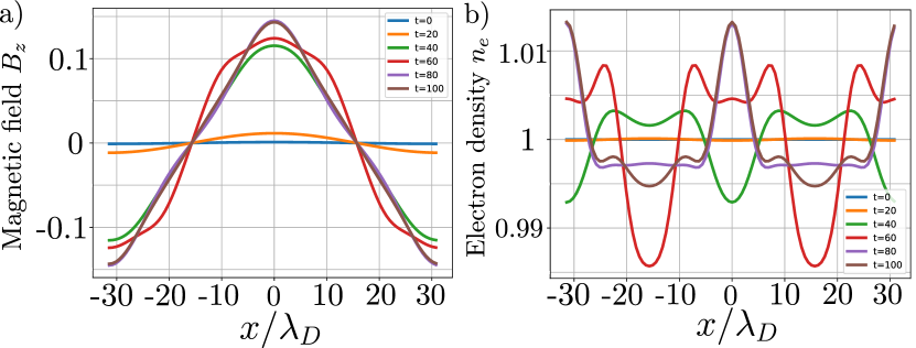
Figure 20: Evolution of (a) magnetic field $B_{z}(x)$ and (b) electron density $n_{e}(x)$, to nonlinear saturation of a single unstable Weibel mode. The mode saturates around $t\omega_{p}\approx 45$. Prior to saturation the magnetic field has a spectrum consisting of only even mode numbers with an apparent power law in logarithmic amplitudes. Since the function is clearly analytic this spectrum is consistent with an elliptic cosine function until nonlinear saturation. It is interesting that this higher-order phenomenon arises even from a single-mode eigenfunction perturbation. The electron holes at saturation are bounded by the maxima of magnetic energy $B^{2}/2\mu_{0}$, or equivalently bounded by the potential wells $A_{y}(x)$.

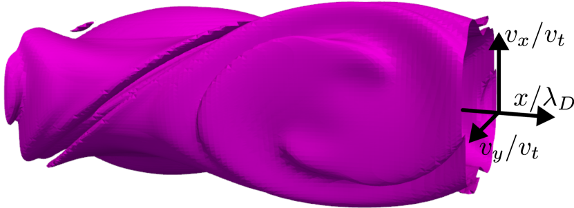
Figure 21: Phase space vortex shown by contour at $0.1\text{max}(f)$ in the coordinates $(x,v_{x},v_{y})$ at saturation of a single Weibel mode. The mid-domain $x$-coordinate corresponds to $x=0$. The magnetic trapping phase space vortex is distinguished from the electrostatic vortex as velocity-dependent since the momentum $p_{y}$ in Eq. 92 is linear in $v_{y}$. In this way the single-mode phase space vortex is antisymmetric, with trapped and passing orbits swapping under $v_{y}\to-v_{y}$. For this reason there is no magnetic trapping along the $v_{y}=0$ plane.

4.5 Saturation of many unstable Weibel modes in two spatial dimensions

Weibel instability is inherently multidimensional as wavevectors oblique to the principal anisotropy axes have comparable growth rates to the principal axes (similar to the multidimensional streaming instability studied in Section 2.7). We consider for example the branch of the dispersion function for the anisotropic Maxwellian given by Eq. 88 with transverse magnetic field out of plane and the longitudinal and transverse electric fields in-plane. The out-of-plane magnetic field allows a reduced 2D2V phase space geometry for reduced continuum-kinetic simulation (Skoutnev et al., (2019)). It should be kept in mind that the instability dynamics are truly three-dimensional just as in the multidimensional Langmuir turbulence simulation of Section 2.7. Figure 22 plots the growth rate as a function of the wavevector $\bm{k}=k_{x}\hat{x}+k_{y}\hat{y}$ of the unstable branch of Eq. 88 for a zero-order bi-Maxwellian of anisotropy $A=3$ and with $v_{t}/c=0.3$.

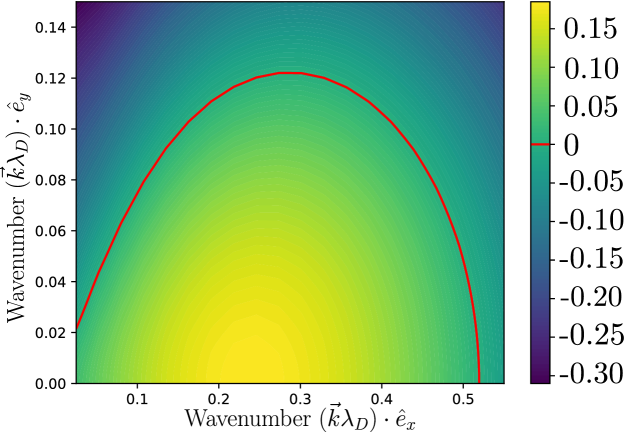
Figure 22: Growth rates of multidimensional Weibel instability as $\text{Im}(\omega)/\omega_{pe}$ for an anisotropic bi-Maxwellian of anisotropy $A=3$ where the electric field is assumed to lie in the $(x,y)$-plane and the first-order transverse magnetic field to be out-of-plane. The higher-temperature direction is assumed to lie in the $\hat{y}$-direction assuming $v_{t}/c=0.3$. The red line identifies marginal stability.

4.5.1 Initialization of two-dimensional multi-mode Weibel instability

The numerical method is summarized in Appendix A and Crews and Shumlak, (2022) with the difference that here Ampere’s law and Faraday’s law are used for the field equations, and are time-integrated in Fourier spectral space with the same third-order Adams-Bashforth multistep method used for the kinetic equation. However there is an important difference in initialization of the unstable modes. In the Vlasov-Poisson system the phase space eigenfunctions are proportional to the scalar potential $\varphi$, yet in the multidimensional Vlasov-Maxwell system the phase space eigenfunctions are related to the electric field eigenfunction $\bm{E}$, a vector quantity. When initializing with phase space eigenfunctions in an electrodynamic problem this vector must be an eigenfunction of the equation $\chi\bm{E}=\zeta^{2}\bm{E}$, as discussed in Section 4.2. In our implementation, for each wavevector the eigenfunction is computed in the rotated frame of the wavevector and then anti-rotated back into the $(x,y)$-plane with components $\bm{E}=E_{x}\hat{x}+E_{y}\hat{y}$. Thus for each desired pair of wavenumbers $(k_{x},k_{y})$ a perturbation is applied as

$$f_{1}=\mathcal{A}\text{Re}\Big{[}\frac{q}{i\omega}\Big{\{}E_{x}\Big{(}\frac{\partial f_{0}}{\partial u}+\frac{v_{x}(\bm{k}\cdot\nabla_{v}f_{0})}{\omega-\bm{k}\cdot\bm{v}}\Big{)}+E_{y}\Big{(}\frac{\partial f_{0}}{\partial v}+\frac{v_{y}(\bm{k}\cdot\nabla_{v}f_{0})}{\omega-\bm{k}\cdot\bm{v}}\Big{)}\Big{\}}e^{i(\bm{k}\cdot\bm{x}+\widetilde{\varphi})}\Big{]}$$ (93)

with $\widetilde{\varphi}$ a randomly chosen phase shift per wavevector and the amplitude $\mathcal{A}=2\times 10^{-3}$. The magnetic field is then initialized as $B_{z}=\zeta^{-1}\hat{k}\times\bm{E}$ where $\zeta$ is the eigenvalue. Higher amplitude than the one-dimensional problem is chosen to reduce time to saturation.

The domain is specified by fundamental wavenumbers $k_{x}\lambda_{D}=0.125$ and $k_{y}\lambda_{D}=0.01$. Physical space is represented with $N_{x}=32$ and $N_{y}=128$ evenly-spaced collocation points, while velocity space is represented as a Cartesian tensor product of linear finite elements with eleven finite elements per velocity axis, each linear element of seventh-order polynomial basis for $(v_{x},v_{y})\in[-11,11]\theta_{u}$. As in Section 2.7 many modes are excited; for each of the first two harmonics of the fundamental wavenumber, namely $nk_{x}\lambda_{D}$ with $n=1,2$, five transverse wavenumbers $\pm mk_{y}\lambda_{D}$ are excited with $m=0,1,2$. The normalized thermal velocity $v_{t}/c=0.3$ and the anisotropy is $A=3$, as in the one-dimensional problem. The simulation is run to $t\omega_{p}=40$ using a time-step of $\Delta t=8\times 10^{-3}$ with an added hyperviscosity $\nu\nabla_{x}^{4}f$ with $\nu=1$ to prevent spectral blocking. Due to the hyperviscosity total energy is conserved only to $\mathcal{O}(10^{-4})$ by the simulation stop time.

4.5.2 Nonlinear simulations of the two-dimensional Weibel instability

Figure 23 shows the energy traces of the electrodynamic field during the linear phase and beyond instability saturation. Nonlinear saturation occurs around $t\omega_{p}=17$, as gauged by the transverse electric field $E_{y}$. The $\hat{x}$-directed electric field energy follows a similar trend as in the one-dimensional problem. Its growth is made up of two effects: linear growth from the initialized oblique modes, and the development of “longitudinal” space charge (filamentation) to second-order in the magnetic field as discussed in Section 4.4. Nonlinear saturation occurs due to the formation of magnetic-trapping electron holes at the boundary between counter-streaming mean flows.

Figure 24 illustrates the dynamics of the multidimensional instability through streamlines of the current density $\bm{j}(x,y)$ and filled contours of its magnitude for three times in the simulation output. Trigonometric interpolation is used to visualize the current density by zero-padding the spectrum and inverse Fourier transformation, as the spectrum is properly resolved up to the chosen spectral cut-off. In Fig. 24b one can observe spiral current streamlines indicating the local production of space charge as the electron density filaments into two-dimensional analogues of the magnetic-trapping electron holes studied in the single-mode problem, also observed in Califano et al., (1997). By the simulation’s end, nonlinear mixing has caused some of the filaments to rotate, as in the multidimensional electrostatic problem considered in Section 2.7, indicating a similar isotropization on averaged scales. Inspection of Fig. 25, which plots the spatially-averaged distribution function $\langle f\rangle_{(x,y)}(v_{x},v_{y})$ at $t\omega_{p}=0$ and $t\omega_{p}=40$ in Figs. 25a,b and in Fig. 25c the trace of the anisotropy parameter $A$, shows the anisotropic Maxwellian to relax towards isotropy through Weibel turbulence. The initial anisotropy $A=3$ is observed to decrease monotonically until at saturation $A\approx 1$, meaning that the saturated state is weakly anisotropic. This persistent anisotropy coexists with the fluctuating turbulent filamentation currents, consistent with the observations of Davidson et al., (1972). Indeed, persistent anisotropy accompanying electron shear flow dynamics in the saturated state is expected for collisionless dynamics (Del Sarto and Pegoraro, (2018)).

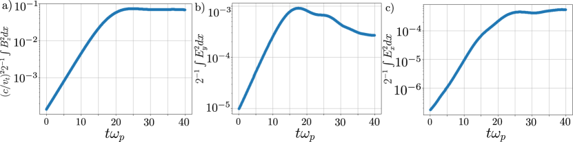
Figure 23: Evolution of domain-integrated energy for (a) the out-of-plane magnetic field $B_{z}$, (b) the electric field transverse to the maximum growth-rate axis, and (c) the electric field parallel to that axis (formerly the longitudinal field of the one-dimensional simulation). A difference from the one-dimensional simulation is a steadily decreasing transverse electric energy rather than a coherent oscillation after saturation time. The $\hat{x}$-directed electric energy increases at a rate faster than the growth of the linear modes due to the same space charge effects as in the single-mode simulation discussed in Section 4.4.

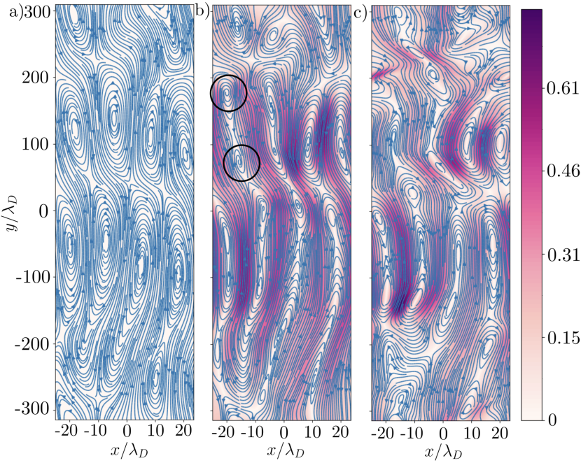
Figure 24: Evolution of current at times (a) $t\omega_{p}=0$, (b) $t\omega_{p}=25$, and (c) $t\omega_{p}=39.5$. Plotted are streamlines of $\bm{j}$ and its magnitude $|\bm{j}|$ as filled contours. Current tends to form closed paths at long wavelength in $y$. The indicated spiral vortices in the streamlines demonstrate rapid local space charge production ($\nabla\cdot\bm{j}\neq 0$) as expected from the filamentation and trapping dynamics of the one-dimensional problem. The large circulating configuration space electron current vortices manifest on small scales as counter-propagating electron streams which sustain a train of magnetic-trapping electron phase space vortices. In this unmagnetized model problem, these structures isotropize from four-dimensional phase space dynamics.

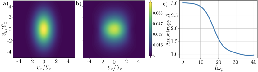
Figure 25: The relaxing spatially-averaged distribution function $\langle f\rangle_{(x,y)}(v_{x},v_{y})$ shown at two times: (a) the initial condition $t\omega_{p}=0$, (b) the stop-time $t\omega_{p}=40$, and in addition (c) the time evolution of the anisotropy parameter $A=\langle v_{y}^{2}\rangle/\langle v_{x}^{2}\rangle-1$. The turbulence of magnetic trapping phase space vortices in the turbulent currents of the saturated instability isotropizes the distribution function. Note that $A=0$ would indicate a fully isotropic distribution, so that the saturated state consists of some degree of anisotropy coexisting with the turbulent wavefield (Davidson et al., (1972)).

5 General discussion

This article has reviewed the theory of phase space eigenfunctions and their application in nonlinear kinetic simulations through detailed examples of the most commonly treated model problems. The initial discussion summarized the kinetic eigenvalue and initial value problems, and it is highlighted that the instabilities identified in Landau’s initial value analysis are indeed true eigenfunctions, and may be utilized as perturbations in nonlinear simulations. Perturbation of a kinetic problem using phase space eigenfunctions provides several benefits, such as a controlled partition of perturbation energy, initialization of perturbations at close-to-nonlinear amplitudes, and measurement of linear instability growth rates up to machine precision unpolluted by linear Landau-damping modes. This method is then applied to the multidimensional streaming instability problem, and extended to more complex problems encountered by researchers in space and fusion plasma physics, namely cyclotron loss-cone instability and electromagnetic Weibel instability.

While by no means an exhaustive overview of the possibilities of kinetic eigenfunctions, a few notable problems are demonstrated to benefit from an eigenfunction approach. The electrostatic problem in a static magnetic field is treated in detail for loss-cone distributions, and new analytic results for the loss-cone dielectric function are presented. Nonlinear saturation of the multi-dimensional Weibel instability of an anisotropic Maxwellian distribution, originally treated by Davidson et al., (1972) with the particle-in-cell method, is revisited and new light shed with a high-order accurate continuum kinetic method. One further simple and important model problem is left for future work, namely pressure anisotropy induced whistler wave emission parallel to the magnetic field.

A few further notes are in order regarding the importance of phase space eigenfunctions in numerical plasma theory. In this work the emphasis is on observing the evolution of the linear eigenfunctions into nonlinear structures as the examined zero-order distributions are far from equilibrium. Another important class of problems are the weakly unstable distributions, which are commonly treated by quasilinear theory. In numerical solutions of quasilinear theory there is no transition to nonlinear structures and the phase space dynamics of the obtained spectra are necessarily those of the eigenfunctions. As another way of phrasing this, one can say that in weak turbulence the linear eigenfunctions contain most of the fluctuation energy. The application of kinetic phase space eigenfunctions to numerically study quasilinear theory potentially offers a multitude of interesting and valuable avenues of further exploration.

Acknowledgements

The authors would like to thank J. B. Coughlin, I. A. M. Datta, A. Ho, E. T. Meier, A. D. Stepanov, Y. Takagaki, W. H. Thomas, and G. V. Vogman for helpful discussions. The information, data, or work presented herein was funded in part by the Air Force Office of Scientific Research under Award No. FA9550–15–1–0271. This material is based upon work supported by the National Science Foundation under Grant No. PHY-2108419.

Appendix A Summary of numerical method

Our numerical method is a combination of the pseudospectral method for spatial fluxes (Boyd, (2001)) with high-order discontinuous Galerkin method for velocity space (Crews and Shumlak, (2022)). The Vlasov-Poisson system is discretized in configuration space by Galerkin projection onto a truncated multi-dimensional Fourier basis, for example $(x,y)\to(k_{n},k_{m})$. That is, if the original kinetic equation is

$$\partial_{t}f+\bm{v}\cdot\nabla_{x}f+\bm{F}\cdot\nabla_{v}f=0$$ (94)

with $\bm{F}$ the vector of momentum fluxes, then the Galerkin-projected kinetic equation is

$$\frac{\partial f_{nm}}{\partial t}+ik_{n}uf_{nm}+ik_{m}vf_{nm}+\nabla_{v}\cdot(\bm{\mathcal{F}}_{nm})=0$$ (95)

with $\bm{\mathcal{F}}_{nm}$ the vector of spectral momentum fluxes. Eq. 95 is discretized by truncating the velocity domain and applying the discontinuous Galerkin method $(u,v)\to(u_{jk},v_{pq})$, with $(j,p)$ the element indices and $(k,q)$ the sub-element indices (that is, the collocation nodes), and a set of basis functions $\psi_{k}$ are chosen. We use the Legendre-Gauss-Lobatto basis (Hesthaven and Warburton, (2007)). The semi-discrete equation obtained is

$$\frac{df_{nmjkpq}}{dt}=\mathcal{N}_{nmjkpq}[f]+\mathcal{L}_{nmjkpq}^{\ell r}f_{nmj\ell pr}$$ (96)

where $\mathcal{N}$ is a nonlinear operator representing the discretized velocity flux divergences, while $\mathcal{L}$ is the advective part of the semi-discrete operator and is linear in $f$. Advection is not linear in $\bm{v}$, but is integrated over the basis functions $\psi_{k}$ to form a linear operator

$$\mathbb{T}_{njk}^{\ell}\equiv-ik_{n}(\bar{v}_{j}I_{k}^{\ell}+J_{m}\langle\psi_{k}|\psi^{s}\rangle^{-1}\langle\xi\psi_{s}|\psi^{\ell}\rangle),$$ (97)

with $\langle\cdot|\cdot\rangle$ an inner product over the reference element with coordinate $\xi\in[-1,1]$, and $\bar{v}_{j}$ the velocity in the midpoint of element $j$ with transformation $v_{j}(\xi)=\bar{v}_{j}+(\Delta v)_{j}\xi/2$ with $(\Delta v)_{j}$ the element width. Then advection is represented by a linear operator

$$\mathcal{L}_{nmjkpq}^{\ell r}f_{nmj\ell pr}\equiv\mathbb{T}_{njk}^{\ell}f_{nmj\ell pq}+\mathbb{T}_{mpq}^{r}f_{nmjkpr}.$$ (98)

Poisson’s equation is solved algebraically in Fourier space, and the velocity fluxes $\mathcal{N}$ are computed by the pseudospectral method. That is, the spectral field and distribution are both zero-padded using Orszag’s two-thirds rule and transformed to nodal values on the spatial collocation points where the fluxes are calculated. The velocity element boundary fluxes are then calculated in $(\bm{x},\bm{v})$ space by upwind method and transformed back to spectral space for time integration. However, element-internal fluxes are calculated in $(\bm{k},\bm{v})$ space by inverse transformation as the spectral symmetry from $\text{Im}(f(\bm{x},\bm{v}))=0$ reduces the operations by a factor of two. Finally, the semi-discrete equation is advanced through $\Delta t=h$ using second-order Strang splitting of linear $\mathcal{L}$ and nonlinear $\mathcal{N}$ fluxes,

$$f^{n+1}=\mathcal{S}[\mathcal{L}]^{h/2}\mathcal{S}[\mathcal{N}]^{h}\mathcal{S}[\mathcal{L}]^{h/2}f^{n}$$ (99)

where $\mathcal{S}[\cdot]$ represents evaluation of the separated operator by any method of approximation. In this simulation the explicit third-order Adams-Bashforth method is used for the nonlinear flux $\mathcal{S}[\mathcal{N}]^{h}$ while advection is advanced implicitly by Crank-Nicholson stepping,

$$\Big{(}\mathcal{S}[\mathcal{L}]^{h}\Big{)}^{\ell r}_{nmjkpq}=\Big{(}I^{\ell}_{njk}-\frac{h}{2}\mathbb{T}^{\ell}_{njk}\Big{)}^{-1}\Big{(}I^{\ell}_{njk}+\frac{h}{2}\mathbb{T}^{\ell}_{njk}\Big{)}\Big{(}I^{r}_{mpq}-\frac{h}{2}\mathbb{T}^{r}_{mpq}\Big{)}^{-1}\Big{(}I^{r}_{mpq}+\frac{h}{2}\mathbb{T}^{r}_{mpq}\Big{)}$$ (100)

with $I_{mpq}^{r}$ the identity matrix $I_{q}^{r}$ for each $(m,n)$. Fractional stepping for advection is advantageous as it reduces the $\mathcal{O}(N^{2})$ operations per cell into two $\mathcal{O}(N)$ operations. The calculation of the nonlinear momentum flux operator $\mathcal{N}$ is treated in Crews, (2022).

Appendix B Polar Fourier integrals of loss-cone distributions

This appendix integrates the ring distribution of Eq. 50 over perpendicular velocities,

$$\mathbb{F}_{n,m,\gamma}(k)\equiv\int_{0}^{\infty}f_{\gamma}(v)J_{n}(kv)J_{m}(kv)2\pi vdv$$ (101)

for integer $n,m$. By this formula one can also determine the integral of products, $J_{n}(v)J_{n}^{\prime}(v)$ etc., by recursion of the derivatives $J_{n}^{\prime}(z)$. The result is that Eq. 101 is a type-${}_{3}F_{3}$ hypergeometric function,

$$\begin{split}\mathbb{F}_{n,m,\gamma}(k)=&\frac{\Gamma(\gamma+\frac{n+m}{2}+1)(k\alpha)^{n+m}}{\Gamma(n+1)\Gamma(m+1)\Gamma(\gamma+1)}\times\\ &{}_{3}F_{3}\genfrac{[}{]}{0.0pt}{}{\frac{n+m}{2}+\frac{1}{2},\frac{n+m}{2}+1,\gamma+\frac{n+m}{2}+1}{n+1,\quad m+1,\quad n+m+1}(-(2k\alpha)^{2})\end{split}$$ (102)

which is equivalently written as a power series with Gamma function coefficients,

$$\mathbb{F}_{n,m,\gamma}(k)=\frac{1}{\Gamma(\gamma+1)}\sum_{\ell=0}^{\infty}\frac{\Gamma(n+m+2\gamma+2\ell+1)}{\Gamma(n+\ell+1)\Gamma(m+\ell+1)\Gamma(n+m+\ell+1)}\frac{(-1)^{\ell}}{\ell!}(k\alpha)^{2\ell+n+m}.$$ (103)

Setting $n=m$ as in electrostatic theory reduces to a more manageable ${}_{2}F_{2}$ function,

$$\mathbb{F}_{n,\gamma}(k)=\frac{\Gamma(\gamma+n+1)(k\alpha)^{2n}}{\Gamma^{2}(n+1)\Gamma(\gamma+1)}{}_{2}F_{2}\genfrac{[}{]}{0.0pt}{}{n+\frac{1}{2},\gamma+n+1}{n+1,2n+1}(-(2k\alpha)^{2})$$ (104)

with the power series for practical computation given in Eq. 54.

B.1 The product of integer-order Bessel functions

The product of integer-order Bessel functions is a generalized ${}_{2}F_{3}$-type hypergeometric,

$$J_{n}(z)J_{m}(z)=\frac{1}{n!m!}\Big{(}\frac{z}{2}\Big{)}^{n+m}{}_{2}F_{3}\genfrac{[}{]}{0.0pt}{}{\frac{n+m}{2}+\frac{1}{2},\frac{n+m}{2}+1}{n+1,m+1,n+m+1}(-z^{2})$$ (105)

which for $n=m$ reduces to a type ${}_{1}F_{2}$ function,

$$J_{n}^{2}(z)=\frac{1}{(n!)^{2}}\Big{(}\frac{z}{2}\Big{)}^{2n}{}_{1}F_{2}\genfrac{[}{]}{0.0pt}{}{n+\frac{1}{2}}{n+1,2n+1}(-z^{2}).$$ (106)

B.1.1 Demonstration of Equation 105

Multiplying term-by-term the power series of $J_{n}$, $J_{m}$ and diagonalizing by $\ell=j+k$,

$$\begin{split}J_{n}(z)J_{m}(z)&=\Big{(}\frac{z}{2}\Big{)}^{n+m}\sum_{j,k=0}^{\infty}\frac{1}{\Gamma(n+k+1)\Gamma(m+j+1)}\frac{(-z^{2}/4)^{j+k}}{j!k!}\\ &=\Big{(}\frac{z}{2}\Big{)}^{n+m}\sum_{\ell=0}^{\infty}\Big{[}\sum_{k=0}^{\infty}\frac{1}{\Gamma(k+n+1)\Gamma(\ell-k+m+1)\Gamma(\ell-k+1)\Gamma(k+1)}\Big{]}\Big{(}\frac{-z^{2}}{4}\Big{)}^{\ell}.\end{split}$$ (107)

Using properties of Pochhammer symbols and Gauss’s hypergeometric theorem,

$$\begin{split}\sum_{k=0}^{\infty}&\frac{1}{\Gamma(k+n+1)\Gamma(\ell-k+m+1)\Gamma(\ell-k+1)\Gamma(k+1)}\\ =&\frac{1}{\Gamma(n+1)\Gamma(\ell+1)\Gamma(\ell+m+1)}{}_{2}F_{1}\genfrac{[}{]}{0.0pt}{}{-\ell,-\ell-m}{n+1}(1)\\ =&\frac{\Gamma(n+m+2\ell+1)}{\Gamma(\ell+1)\Gamma(m+\ell+1)\Gamma(n+\ell+1)\Gamma(n+m+\ell+1)}\end{split}$$ (108)

one obtains a single summation for $J_{n}(z)J_{m}(z)$,

$$J_{n}(z)J_{m}(z)=\Big{(}\frac{z}{2}\Big{)}^{n+m}\sum_{\ell=0}^{\infty}\frac{\Gamma(n+m+2\ell+1)}{\Gamma(m+\ell+1)\Gamma(n+\ell+1)\Gamma(n+m+\ell+1)}\frac{(-z^{2}/4)^{\ell}}{\ell!}.$$ (109)

The numerator factorial is then written in Pochhammer symbols by the formulas

$$(x+\ell)_{\ell} =\frac{(x)_{2\ell}}{(x)_{\ell}},$$ (110)

$$(x)_{2\ell} =2^{2\ell}\Big{(}\frac{x}{2}\Big{)}_{\ell}\Big{(}\frac{1+x}{2}\Big{)}_{\ell},$$ (111)

yielding a series identical to Eq. 105 and proving the identity,

$$J_{n}(z)J_{m}(z)=\frac{1}{n!m!}\Big{(}\frac{z}{2}\Big{)}^{n+m}\sum_{\ell=0}^{\infty}\frac{\big{(}\frac{n+m}{2}+\frac{1}{2}\big{)}_{\ell}\big{(}\frac{n+m}{2}+1\big{)}_{\ell}}{(m+1)_{\ell}(n+1)_{\ell}(n+m+1)_{\ell}}\frac{(-z^{2})^{\ell}}{\ell!}.$$ (112)

B.2 Integration of Eq. 105 with a loss-cone distribution

Having developed the product of two Bessel functions in terms of a single entire function the integration over perpendicular velocities is now shown to be Eq. 102.

B.2.1 Demonstration of Eq. 102

The ring distribution $f_{\gamma}(v)$ is combined with Eq. 112 and integrated term-by-term,

$$\begin{split}\mathbb{F}_{n,m,\gamma}(k)=\frac{k^{n+m}}{n!m!\gamma!(\alpha^{2})^{\gamma+1}}\Big{(}\frac{k}{2}\Big{)}^{n+m}\sum_{\ell=0}^{\infty}&\frac{\big{(}\frac{n+m}{2}+\frac{1}{2}\big{)}_{\ell}\big{(}\frac{n+m}{2}+1\big{)}_{\ell}}{(m+1)_{\ell}(n+1)_{\ell}(n+m+1)_{\ell}}\frac{(-k^{2})^{\ell}}{\ell!}\times\\ &\int_{0}^{\infty}v^{2(\ell+\gamma+\frac{n+m}{2})}e^{-v^{2}/\alpha^{2}}2vdv.\end{split}$$ (113)

The interior integral is Euler’s form of the Gamma function upon substitution $u=\frac{v^{2}}{\alpha^{2}}$,

$$\begin{split}\mathbb{F}_{n,m,\gamma}=&\frac{\Gamma(\gamma+\frac{n+m}{2}+1)}{\Gamma(n+1)\Gamma(m+1)\Gamma(\gamma+1)}(k\alpha)^{n+m}\times\\ &\sum_{\ell=0}^{\infty}\frac{\big{(}\frac{n+m}{2}+\frac{1}{2}\big{)}_{\ell}\big{(}\frac{n+m}{2}+1\big{)}_{\ell}(\gamma+\frac{n+m}{2}+1)_{\ell}}{(m+1)_{\ell}(n+1)_{\ell}(n+m+1)_{\ell}}\frac{(-4\alpha^{2}k^{2})^{\ell}}{\ell!}.\end{split}$$ (114)

The series is a hypergeometric function of type-${}_{3}F_{3}$, demonstrating Eq. 102. While the form of the integral as a type-${}_{3}F_{3}$ function reveals connections to the theory of special functions, in a practical computation it is more practical to use the Gamma function form of the series as in Eq. 103.

Appendix C The Harris dispersion function in loss-cone plasmas

This appendix demonstrates Eqs. 58 and 59 for electrostatic modes in a plasma with zero-order cyclotron orbits distributed as a loss cone, beginning from Eq. 42 known as the Harris dispersion function. We begin by constructing the function in closed form as a hypergeometric function, and then consider a convenient trigonometric integral form by calculation of the loss cone’s Hankel transform. These forms of the dielectric function $\varepsilon(\omega,k_{\perp})$, which sum the contribution of the cyclotron resonances to all orders, enable precise numerics to determine eigenvalues in continuum kinetic simulations.

C.1 The perpendicular wave dielectric function in closed form

We demonstrate Eq. 58 for the closed form of the dielectric function for perpendicular cyclotron waves in a loss-cone distributed plasma using the Lerche-Newberger summation theorem (Lerche, (1974); Newberger, (1982)), which sums the Bessel series in Eqs. 40 and 41 to all orders in the cyclotron harmonics,

$$\Upsilon_{2} =\sum_{n=-\infty}^{\infty}\frac{n}{\omega^{\prime}-n}J_{n}^{2}(\beta)=\frac{\pi\omega^{\prime}}{\sin(\pi\omega^{\prime})}J_{\omega^{\prime}}(\beta)J_{-\omega^{\prime}}(\beta)-1$$ (115)

$$\Lambda_{2} =\sum_{n=-\infty}^{\infty}\frac{1}{\omega^{\prime}-n}J_{n}^{2}(\beta)=\frac{\pi}{\sin(\pi\omega^{\prime})}J_{\omega^{\prime}}(\beta)J_{-\omega^{\prime}}(\beta)$$ (116)

with each sum limiting to a product of Bessel functions $J_{z}(\beta)J_{-z}(\beta)$ of complex order. Here the auxiliary quantities are $\omega^{\prime}=(\omega-k_{\parallel}v_{\parallel})/\omega_{c}$ and $\beta=k_{\perp}v_{\perp}/\omega_{c}$. The polar velocity-space integrals over $v_{\perp}$, when considering the closed forms of Eqs. 115 and 116, result in a generalized hypergeometric function (see the following for a demonstration),

$$\frac{1}{2^{\gamma}\alpha^{2\gamma+2}\Gamma(\gamma+1)}\int_{0}^{\infty}v^{2j+1}e^{-v^{2}/2\alpha^{2}}\frac{\pi\omega}{\sin(\pi\omega)}J_{\omega}(qv)J_{-\omega}(qv)dv={}_{2}F_{2}\genfrac{[}{]}{0.0pt}{}{\frac{1}{2},\quad\gamma+1}{1+\omega,1-\omega}(-2(\alpha q)^{2}).$$ (117)

First note that with $k_{\parallel}=0$ the Harris dispersion function is

$$\varepsilon(\omega,k_{\perp})=1+\Big{(}\frac{\omega_{p}}{\omega_{c}}\Big{)}^{2}\frac{1}{(k\lambda_{D})^{2}}\int_{0}^{\infty}\frac{\Upsilon_{2}}{v_{\perp}}\frac{\partial f_{0}}{\partial v_{\perp}}2\pi v_{\perp}dv_{\perp}.$$ (118)

Using the identity Eq. 117, and the recurrence relation for $f_{\gamma}(v_{\perp})$ of Eq. 52, one obtains

$$\int_{0}^{\infty}\frac{\Upsilon_{2}}{v_{\perp}}\frac{\partial f_{0}}{\partial v_{\perp}}2\pi v_{\perp}dv_{\perp}={}_{2}F_{2}\genfrac{[}{]}{0.0pt}{}{\frac{1}{2},\quad\gamma+1}{1+\omega^{\prime},1-\omega^{\prime}}(-2(k_{\perp}r_{L})^{2})-{}_{2}F_{2}\genfrac{[}{]}{0.0pt}{}{\frac{1}{2},\quad\quad\gamma}{1+\omega^{\prime},1-\omega^{\prime}}(-2(k_{\perp}r_{L})^{2})$$ (119)

which was to be shown.

C.1.1 Demonstration of Eq. 117

Observe that term-by-term multiplication of the power series for both $J_{\omega}$ and $J_{-\omega}$, and diagonalization of the double sum with $\ell=m+k$, leads to the expression

$$\frac{\pi\omega}{\sin(\pi\omega)}J_{\omega}(z)J_{-\omega}(z) =\sum_{m=0}^{\infty}\sum_{k=0}^{\infty}\frac{\Gamma(1+\omega)\Gamma(1-\omega)}{\Gamma(m+\omega+1)\Gamma(k-\omega+1)}\frac{(-1)^{m+k}}{m!k!}\Big{(}\frac{z}{2}\Big{)}^{2(m+k)}$$ (120)

$$=\sum_{\ell=0}^{\infty}\Big{[}\sum_{m=0}^{\infty}\frac{\Gamma(1+\omega)\Gamma(1-\omega)}{\Gamma(m+\omega+1)\Gamma(\ell-m-\omega+1)}\frac{1}{m!(\ell-m)!}\Big{]}(-1)^{\ell}\Big{(}\frac{z}{2}\Big{)}^{2\ell}$$ (121)

having used Euler’s reflection formula $\pi z\csc(\pi z)=\Gamma(1+z)\Gamma(1-z)$ with $\Gamma(z)$ the Gamma function. Recall an identity for the rising factorial $(z)_{n}$ (or Pochhammer symbol),

$$(z)_{n}=\frac{\Gamma(z+n)}{\Gamma(z)}=(-1)^{n}\frac{\Gamma(z+1)}{\Gamma(z-n+1)}$$ (122)

as well as Gauss’s hypergeometric summation theorem,

$${}_{2}F_{1}\genfrac{[}{]}{0.0pt}{}{a,b}{c}(1)=\frac{\Gamma(c)\Gamma(c-a-b)}{\Gamma(c-a)\Gamma(c-b)},\quad\text{Re}(c)>\text{Re}(a+b).$$ (123)

Application of Eqs. 122 and 123 to Eq. 121 shows that the inner summation becomes

$$\sum_{m=0}^{\infty}\frac{\Gamma(1+\omega)\Gamma(1-\omega)}{\Gamma(m+\omega+1)\Gamma(\ell-m-\omega+1)}\frac{1}{m!(\ell-m)!}=2^{2\ell}\frac{(\frac{1}{2})_{\ell}}{(1+\omega)_{\ell}(1-\omega)_{\ell}}\frac{1}{\ell!}.$$ (124)

Therefore, the function expressed by the Lerche-Newberger theorem is a hypergeometric,

$$\frac{\pi\omega}{\sin(\pi\omega)}J_{\omega}(z)J_{-\omega}(z)=\sum_{\ell=0}^{\infty}\frac{(-1)^{\ell}(\frac{1}{2})_{\ell}}{(1+\omega)_{\ell}(1-\omega)_{\ell}}\frac{z^{2\ell}}{\ell!}={}_{1}F_{2}\genfrac{[}{]}{0.0pt}{}{\frac{1}{2}}{1+\omega,1-\omega}(-z^{2}).$$ (125)

Now to compute the integral, the power series in Eq. 125 is integrated term-by-term,

$$\frac{1}{2^{\gamma}\alpha^{2\gamma+2}\Gamma(\gamma+1)}\int_{0}^{\infty} v^{2j+1}e^{-v^{2}/2\alpha^{2}}\frac{\pi\omega}{\sin(\pi\omega)}J_{\omega}(qv)J_{-\omega}(qv)dv=$$ (126)

$$=\frac{1}{2^{\gamma}\alpha^{2\gamma+2}\Gamma(\gamma+1)}\int_{0}^{\infty}v^{2\gamma+1}e^{-v^{2}/2\alpha^{2}}{}_{1}F_{2}\genfrac{[}{]}{0.0pt}{}{\frac{1}{2}}{1+\omega,1-\omega}(-(qv)^{2})dv$$ (127)

$$=\sum_{\ell=0}^{\infty}\frac{(\frac{1}{2})_{\ell}(\gamma+1)_{\ell}}{(1+\omega)_{\ell}(1-\omega)_{\ell}}\frac{(-2(\alpha q)^{2})^{\ell}}{\ell!}$$ (128)

as the coefficients reduce to Euler’s integral $\Gamma(1+z)=\int_{0}^{\infty}x^{z}e^{-x}dx$, establishing Eq. 117.

C.2 The trigonometric form of the dielectric function

The preceding closed form as a hypergeometric function of complex order is of theoretical interest as it connects the characteristic frequencies to the theory of special functions. However, at the present stage of development of scientific computing libraries there are limited options for hypergeometric functions with complex index. For this reason the dielectric function is alternatively represented as a trigonometric integral (Tataronis and Crawford, 1970a ; Vogman et al., (2014); Datta et al., (2021)),

$$\varepsilon(\omega,k)=1+\frac{\omega_{p}^{2}}{\omega_{c}^{2}}\int_{0}^{\pi}\frac{\sin(\theta)\sin(\theta\omega)}{\sin(\pi\omega)}\Big{[}\int_{0}^{\infty}f_{\perp}(v)J_{0}(\lambda(\theta)v)2\pi vdv\Big{]}d\theta$$ (129)

with $\lambda=2k\cos(\theta/2)/\omega_{c}$. The inner integration is an azimuthally symmetric polar Fourier transform, or zero-order Hankel transform $\mathcal{H}_{0}[f(r);k]=\int_{0}^{\infty}f(r)J_{0}(kr)rdr$. The Hankel transform has a Fourier-multiplier property with the radial Laplacian,

$$\mathcal{H}_{0}[r^{2n}f(r);k]=(-\nabla_{k}^{2})^{n}\mathcal{H}_{0}[f(r);k].$$ (130)

Further, the coefficients of successive radial Laplacians of the Gaussian function are precisely the Laguerre polynomials,

$$(\nabla_{k}^{2})^{n}[\exp(-\alpha^{2}k^{2}/2)]=(-2\alpha^{2})^{n}L_{n}(\alpha^{2}k^{2}/2)\exp(-\alpha^{2}k^{2}/2).$$ (131)

Therefore the Hankel transform of $f_{\gamma}(v)$ is the family of polar Hermite functions

$$\mathcal{H}_{0}[f_{\gamma}(v);q]=L_{\gamma}\Big{(}\frac{\alpha^{2}q^{2}}{2}\Big{)}\exp\Big{(}-\frac{\alpha^{2}q^{2}}{2}\Big{)}.$$ (132)

Substitution of Eq. 132 into Eq. 129 gives Eq. 59, as was to be shown.

References

- Balescu, (1997) Balescu, R. (1997). Statistical dynamics: matter out of equilibrium. World Scientific.
- Barnes and Chacón, (2021) Barnes, D. C. and Chacón, L. (2021). Finite spatial-grid effects in energy-conserving particle-in-cell algorithms. Computer Physics Communications, 258:107560.
- Bernstein, (1958) Bernstein, I. B. (1958). Waves in a plasma in a magnetic field. Physical Review, 109(1):10.
- Bertrand and Feix, (1968) Bertrand, P. and Feix, M. R. (1968). Nonlinear electron plasma oscillation: the “water bag model”. Physics Letters A, 28(1):68–69.
- Birdsall and Langdon, (1991) Birdsall, C. K. and Langdon, A. B. (1991). Plasma Physics via Computer Simulation. Series in Plasma Physics and Fluid Dynamics. Taylor & Francis.
- Bohm and Gross, (1949) Bohm, D. and Gross, E. P. (1949). Theory of plasma oscillations. A. Origin of medium-like behavior. Phys. Rev., 75.
- Boyd, (2001) Boyd, J. P. (2001). Chebyshev and Fourier spectral methods. Courier Corporation.
- Bratanov et al., (2013) Bratanov, V., Jenko, F., Hatch, D., and Brunner, S. (2013). Aspects of linear Landau damping in discretized systems. Physics of Plasmas, 20(2):022108.
- Cagas et al., (2017) Cagas, P., Hakim, A., Scales, W., and Srinivasan, B. (2017). Nonlinear saturation of the Weibel instability. Physics of Plasmas, 24(11):112116.
- Califano et al., (1997) Califano, F., Pegoraro, F., and Bulanov, S. V. (1997). Spatial structure and time evolution of the Weibel instability in collisionless inhomogeneous plasmas. Physical review E, 56(1):963.
- Case, (1959) Case, K. M. (1959). Plasma oscillations. Annals of physics, 7(3):349–364.
- Che, (2016) Che, H. (2016). Electron two-stream instability and its application in solar and heliophysics. Modern Physics Letters A, 31(19):1630018.
- Cheng and Knorr, (1976) Cheng, C. Z. and Knorr, G. (1976). The integration of the Vlasov equation in configuration space. Journal of Computational Physics, 22(3):330–351.
- Choi et al., (2021) Choi, B., Christlieb, A., and Wang, Y. (2021). High-dimensional sparse Fourier algorithms. Numerical Algorithms, 87:161–186.
- Conner and Wilson, (1994) Conner, J. W. and Wilson, H. R. (1994). Survey of theories of anomalous transport. Plasma physics and controlled fusion, 36(5):719.
- Crews, (2022) Crews, D. W. (2022). Numerical simulation of collisionless kinetic plasma turbulence. PhD thesis, University of Washington.
- Crews et al., (2024) Crews, D. W., Datta, I. A. M., Meier, E. T., and Shumlak, U. (2024). The Kadomtsev pinch revisited for sheared-flow-stabilized Z-pinch modeling. Revised manuscript submitted for consideration in IEEE TPS.
- Crews and Shumlak, (2022) Crews, D. W. and Shumlak, U. (2022). On the validity of quasilinear theory applied to the electron bump-on-tail instability. Physics of Plasmas, 29(4):043902.
- Datta et al., (2021) Datta, I. A. M., Crews, D. W., and Shumlak, U. (2021). Electromagnetic extension of the Dory–Guest–Harris instability as a benchmark for Vlasov–Maxwell continuum kinetic simulations of magnetized plasmas. Physics of Plasmas, 28(7):072112.
- Datta and Shumlak, (2023) Datta, I. A. M. and Shumlak, U. (2023). Computationally efficient high-fidelity plasma simulations by coupling multi-species kinetic and multi-fluid models on decomposed domains. Journal of Computational Physics, 483:112073.
- Davidson et al., (1972) Davidson, R. C., Hammer, D. A., Haber, I., and Wagner, C. E. (1972). Nonlinear development of electromagnetic instabilities in anisotropic plasmas. The Physics of Fluids, 15(2):317–333.
- Del Sarto and Pegoraro, (2018) Del Sarto, D. and Pegoraro, F. (2018). Shear-induced pressure anisotropization and correlation with fluid vorticity in a low collisionality plasma. Monthly notices of the royal astronomical society, 475(1):181–192.
- Dodin, (2022) Dodin, I. Y. (2022). Quasilinear theory for inhomogeneous plasma. Journal of Plasma Physics, 88(4):905880407.
- Dory et al., (1965) Dory, R. A., Guest, G. E., and Harris, E. G. (1965). Unstable electrostatic plasma waves propagating perpendicular to a magnetic field. Physical Review Letters, 14(5):131.
- Drummond and Rosenbluth, (1962) Drummond, W. E. and Rosenbluth, M. N. (1962). Anomalous Diffusion Arising from Microinstabilities in a Plasma. The Physics of Fluids, 5(12):1507–1513.
- Dyabilin and Razumova, (2015) Dyabilin, K. S. and Razumova, K. A. (2015). Thermodynamic approach to the interpretation of self-consistent pressure profiles in a tokamak. Plasma Physics Reports, 41:685–695.
- Einkemmer, (2019) Einkemmer, L. (2019). A performance comparison of semi-Lagrangian discontinuous Galerkin and spline based Vlasov solvers in four dimensions. Journal of Computational Physics, 376:937–951.
- Escande, (2016) Escande, D. F. (2016). Contributions of plasma physics to chaos and nonlinear dynamics. Plasma Physics and Controlled Fusion, 58(11):113001.
- Ewart et al., (2022) Ewart, R. J., Brown, A., Adkins, T., and Schekochihin, A. A. (2022). Collisionless relaxation of a Lynden-Bell plasma. Journal of Plasma Physics, 88(5):925880501.
- Fox et al., (2013) Fox, W., Fiksel, G., Bhattacharjee, A., Chang, P.-Y., Germaschewski, K., Hu, S. X., and Nilson, P. M. (2013). Filamentation instability of counterstreaming laser-driven plasmas. Physical review letters, 111(22):225002.
- Fried and Conte, (1961) Fried, B. D. and Conte, S. D. (1961). The plasma dispersion function: the Hilbert transform of the Gaussian. Academic press.
- Glasser and Qin, (2020) Glasser, A. S. and Qin, H. (2020). The geometric theory of charge conservation in particle-in-cell simulations. Journal of Plasma Physics, 86(3):835860303.
- Gradshteyn and Ryzhik, (2015) Gradshteyn, I. S. and Ryzhik, I. M. (2015). Table of Integrals, Series, and Products. Academic Press, Seventh edition.
- Gurnett and Bhattacharjee, (2017) Gurnett, D. A. and Bhattacharjee, A. (2017). Introduction to plasma physics: With space, laboratory and astrophysical applications. Cambridge University Press.
- He et al., (2016) He, Y., Sun, Y., Qin, H., and Liu, J. (2016). Hamiltonian particle-in-cell methods for Vlasov-Maxwell equations. Physics of Plasmas, 23(9):092108.
- Heath et al., (2012) Heath, R. E., Gamba, I. M., Morrison, P. J., and Michler, C. (2012). A discontinuous Galerkin method for the Vlasov–Poisson system. Journal of Computational Physics, 231(4):1140–1174.
- Heninger and Morrison, (2018) Heninger, J. M. and Morrison, P. J. (2018). An integral transform technique for kinetic systems with collisions. Physics of Plasmas, 25(8):082118.
- Hesthaven and Warburton, (2007) Hesthaven, J. S. and Warburton, T. (2007). Nodal discontinuous Galerkin methods: algorithms, analysis, and applications. Springer Science & Business Media.
- Hill et al., (2005) Hill, J. M., Key, M. H., Hatchett, S. P., and Freeman, R. R. (2005). Beam-Weibel filamentation instability in near-term and fast-ignition experiments. Physics of plasmas, 12(8):082304.
- Ho et al., (2018) Ho, A., Datta, I. A. M., and Shumlak, U. (2018). Physics-based-adaptive plasma model for high-fidelity numerical simulations. Frontiers in Physics, 6:105.
- Huntington et al., (2015) Huntington, C. M., Fiuza, F., Ross, J. S., Zylstra, A. B., Drake, R. P., Froula, D. H., Gregori, G., Kugland, N. L., Kuranz, C. C., Levy, M. C., et al. (2015). Observation of magnetic field generation via the Weibel instability in interpenetrating plasma flows. Nature Physics, 11(2):173–176.
- Hutchinson, (2020) Hutchinson, I. H. (2020). Particle trapping in axisymmetric electron holes. Journal of Geophysical Research: Space Physics, 125(8):e2020JA028093.
- Hutchinson, (2021) Hutchinson, I. H. (2021). Synthetic multidimensional plasma electron hole equilibria. Physics of Plasmas, 28(6):062306.
- Ichimaru, (1992) Ichimaru, S. (1992). Statistical Plasma Physics, Volume I: Basic Principles. CRC Press.
- Kraus et al., (2017) Kraus, M., Kormann, K., Morrison, P., and Sonnendrücker, E. (2017). Gempic: geometric electromagnetic particle-in-cell methods. Journal of Plasma Physics, 83(4):905830401.
- Landau, (1946) Landau, L. D. (1946). On the vibrations of the electronic plasma. J. Phys. USSR, 10(26).
- Landau and Lifshitz, (1946) Landau, L. D. and Lifshitz, E. M. (1946). Electrodynamics of continuous media. Pergamon press Oxford.
- Lenard and Bernstein, (1958) Lenard, A. and Bernstein, I. B. (1958). Plasma oscillations with diffusion in velocity space. Physical Review, 112(5):1456.
- Lerche, (1974) Lerche, I. (1974). A note on summing series of Bessel functions occurring in certain plasma astrophysical situations. Astrophysical Journal, Vol. 190, pp. 165-166 (1974), 190:165–166.
- Leubner, (2004) Leubner, M. P. (2004). Fundamental issues on kappa-distributions in space plasmas and interplanetary proton distributions. Physics of Plasmas, 11(4):1308–1316.
- Leubner and Schupfer, (2001) Leubner, M. P. and Schupfer, N. (2001). A general kinetic mirror instability criterion for space applications. Journal of Geophysical Research: Space Physics, 106(A7):12993–12998.
- Livadiotis and McComas, (2023) Livadiotis, G. and McComas, D. J. (2023). Entropy defect in thermodynamics. Scientific Reports, 13(1):9033.
- Mace, (2004) Mace, R. L. (2004). Generalized electron Bernstein modes in a plasma with a kappa velocity distribution. Physics of Plasmas, 11(2):507–522.
- Mace and Hellberg, (2009) Mace, R. L. and Hellberg, M. A. (2009). A new formulation and simplified derivation of the dispersion function for a plasma with a kappa velocity distribution. Physics of Plasmas, 16(7):072113.
- Mahajan and Hazeltine, (2000) Mahajan, S. M. and Hazeltine, R. D. (2000). Sheared-flow generalization of the Harris sheet. Physics of Plasmas, 7(4):1287–1293.
- Morrison, (2000) Morrison, P. J. (2000). Hamiltonian description of vlasov dynamics: action-angle variables for the continuous spectrum. Transport theory and statistical physics, 29(3-5):397–414.
- Morrison, (2017) Morrison, P. J. (2017). Structure and structure-preserving algorithms for plasma physics. Physics of Plasmas, 24(5):055502.
- Morrison and Pfirsch, (1992) Morrison, P. J. and Pfirsch, D. (1992). Dielectric energy versus plasma energy, and Hamiltonian action-angle variables for the Vlasov equation. Physics of Fluids B: Plasma Physics, 4(10):3038–3057.
- Morse and Nielson, (1971) Morse, R. L. and Nielson, C. W. (1971). Numerical simulation of the Weibel instability in one and two dimensions. The Physics of Fluids, 14(4):830–840.
- Mouhot and Villani, (2011) Mouhot, C. and Villani, C. (2011). On Landau damping. Acta Mathematica, 207(1):29 – 201.
- Newberger, (1982) Newberger, B. S. (1982). New sum rule for products of Bessel functions with application to plasma physics. Journal of Mathematical Physics, 23(7):1278–1281.
- Ng et al., (1999) Ng, C. S., Bhattacharjee, A., and Skiff, F. (1999). Kinetic eigenmodes and discrete spectrum of plasma oscillations in a weakly collisional plasma. Physical review letters, 83(10):1974.
- Nicholson, (1983) Nicholson, D. R. (1983). Introduction to plasma theory. Wiley New York.
- Penrose, (1960) Penrose, O. (1960). Electrostatic Instabilities of a Uniform Non‐Maxwellian Plasma. The Physics of Fluids, 3(2):258–265.
- Perse et al., (2021) Perse, B., Kormann, K., and Sonnendrücker, E. (2021). Geometric Particle-in-Cell Simulations of the Vlasov–Maxwell System in Curvilinear Coordinates. SIAM Journal on Scientific Computing, 43(1):B194–B218.
- Pierrard and Lazar, (2010) Pierrard, V. and Lazar, M. (2010). Kappa distributions: Theory and applications in space plasmas. Solar physics, 267:153–174.
- Pokhotelov et al., (2004) Pokhotelov, O. A., Sagdeev, R. Z., Balikhin, M. A., and Treumann, R. A. (2004). Mirror instability at finite ion-Larmor radius wavelengths. Journal of Geophysical Research: Space Physics, 109(A9).
- Pokhotelov et al., (2002) Pokhotelov, O. A., Treumann, R. A., Sagdeev, R. Z., Balikhin, M. A., Onishchenko, O. G., Pavlenko, V. P., and Sandberg, I. (2002). Linear theory of the mirror instability in non-Maxwellian space plasmas. Journal of Geophysical Research: Space Physics, 107(A10):SMP–18.
- Rosenbluth and Post, (1965) Rosenbluth, M. N. and Post, R. F. (1965). High‐Frequency Electrostatic Plasma Instability Inherent to “Loss‐Cone” Particle Distributions. The Physics of Fluids, 8(3):547–550.
- Rudakov and Tsytovich, (1978) Rudakov, L. I. and Tsytovich, V. N. (1978). Strong Langmuir turbulence. Physics Reports, 40(1):1–73.
- Schamel, (2023) Schamel, H. (2023). Pattern formation in Vlasov–Poisson plasmas beyond Landau caused by the continuous spectra of electron and ion hole equilibria. Reviews of Modern Plasma Physics, 7(1):11.
- Sharma and Bhatnagar, (1976) Sharma, S. R. and Bhatnagar, T. N. (1976). Wave propagation along an arbitrary direction in a bi-maxwellian plasma. Plasma Physics, 18(2):95.
- Short and Simon, (2002) Short, R. W. and Simon, A. (2002). Damping of perturbations in weakly collisional plasmas. Physics of Plasmas, 9(8):3245–3253.
- Shukla et al., (2018) Shukla, N., Vieira, J., Muggli, P., Sarri, G., Fonseca, R., and Silva, L. (2018). Conditions for the onset of the current filamentation instability in the laboratory. Journal of Plasma Physics, 84(3).
- Skoutnev et al., (2019) Skoutnev, V., Hakim, A., Juno, J., and TenBarge, J. M. (2019). Temperature-dependent Saturation of Weibel-type Instabilities in Counter-streaming Plasmas. The Astrophysical Journal Letters, 872(2):L28.
- Stix, (1992) Stix, T. H. (1992). Waves in plasmas. Springer Science & Business Media.
- Taggart et al., (1972) Taggart, K. A., Godrey, B. B., Rhoades Jr, C. E., and Ives, H. C. (1972). Second-Order Effects in the Weibel Instability. Physical Review Letters, 29(26):1729.
- (78) Tataronis, J. A. and Crawford, F. W. (1970a). Cyclotron harmonic wave propagation and instabilities: I. Perpendicular propagation. Journal of Plasma Physics, 4(2):231–248.
- (79) Tataronis, J. A. and Crawford, F. W. (1970b). Cyclotron harmonic wave propagation and instabilities: II. Oblique propagation. Journal of Plasma Physics, 4(2):249–264.
- Tzoufras et al., (2006) Tzoufras, M., Ren, C., Tsung, F. S., Tonge, J. W., Mori, W. B., Fiore, M., Fonseca, R., and Silva, L. O. (2006). Space-charge effects in the current-filamentation or Weibel instability. Physical review letters, 96(10):105002.
- van Kampen, (1955) van Kampen, N. G. (1955). On the theory of stationary waves in plasmas. Physica, 21(6-10):949–963.
- Vedenov, (1963) Vedenov, A. A. (1963). Quasi-linear plasma theory (theory of a weakly turbulent plasma). Journal of Nuclear Energy. Part C, Plasma Physics, Accelerators, Thermonuclear Research, 5(3):169.
- Vogman et al., (2014) Vogman, G. V., Colella, P., and Shumlak, U. (2014). Dory–Guest–Harris instability as a benchmark for continuum kinetic Vlasov–Poisson simulations of magnetized plasmas. Journal of Computational Physics, 277:101–120.
- (84) Weibel, E. S. (1959a). Spontaneously Growing Transverse Waves in a Plasma Due to an Anisotropic Velocity Distribution. Phys. Rev. Lett., 2:83–84.
- (85) Weibel, E. S. (1959b). Spontaneously growing transverse waves in a plasma due to an anisotropic velocity distribution. Physical Review Letters, 2(3):83.
- Yoon, (2007) Yoon, P. H. (2007). Spontaneous thermal magnetic field fluctuation. Physics of plasmas, 14(6).
- Yoon and Lui, (2006) Yoon, P. H. and Lui, A. T. Y. (2006). Quasi-linear theory of anomalous resistivity. Journal of Geophysical Research: Space Physics, 111(A2).
- Zhdankin, (2023) Zhdankin, V. (2023). Dimensional measures of generalized entropy. Journal of Physics A: Mathematical and Theoretical, 56(38):385002.