The dynamics and gravitational-wave signal of a binary flying closely by a Kerr supermassive black hole

Abstract

Recent astrophysical models predict that stellar-mass binary black holes (BBHs) could form and coalesce within a few gravitational radii of a supermassive black hole (SMBH). Detecting the gravitational waves (GWs) from such systems requires numerical tools which can track the dynamics of the binaries while capturing all the essential relativistic effects. This work develops upon our earlier study of a BBH moving along a circular orbit in the equatorial plane of a Kerr SMBH. Here we modify the numerical method to simulate a BBH falling toward the SMBH along a parabolic orbit of arbitrary inclination with respect to the equator. By tracking the evolution in a frame freely falling alongside the binary, we find that the eccentricity of the BBH is more easily excited than it is in the previous equatorial case, and that the cause is the asymmetry of the tidal tensor imposed on the binary when the binary moves out of the equatorial plane. Since the eccentricity reaches maximum around the same time that the BBH becomes the closest to the SMBH, multi-band GW bursts could be produced which are simultaneously detectable by the space- and ground-based detectors. We show that the effective spins of such GW events also undergo significant variation due to the rapid reorientation of the inner BBHs during their interaction with SMBHs. These results demonstrate the richness of three-body dynamics in the region of strong gravity, and highlight the necessity of building new numerical tools to simulate such systems.

1 Introduction

The interaction between supermassive black holes (SMBHs) and binary compact objects, such as stellar-mass binary black holes (BBHs) or double neutron stars (DNSs), can produce various types of gravitational-wave (GW) sources. (i) If a BBH penetrates deeply into the potential well of a SMBH, it is likely tidally disrupted, and the corresponding distance from the SMBH is called the “tidal radius” (Hills, 1988). In many cases, the tidal disruption will leave one of the stellar-mass black holes (BHs) tightly bound to the SMBH, forming a GW source known as the extreme-mass-ratio inspiral (Miller et al., 2005), which is one of the major targets of the Laser Interferometer Space Antenna (LISA, Amaro-Seoane et al., 2023). (ii) Later numerical simulations showed that not all BBHs reaching the tidal radius of a SMBH are disrupted. A substantial fraction can survive, but the eccentricities of the surviving binaries can be excited to large values during the tidal interaction (Addison et al., 2019; Fernández & Kobayashi, 2019). The high eccentricity enhances GW radiation, causing the binaries to coalesce later and become potential targets of the Laser Interferometer Gravitational-wave Observatory (LIGO) and the Virgo detectors (The LIGO Scientific Collaboration & the Virgo Collaboration, 2019, 2020; Ligo Scientific Collaboration et al., 2023). (iii) If the distance is not as close as the tidal radius (and not significantly larger either), the interaction could result in a capture of the binary by the SMBH (Hills, 1991). The captured binary could also be driven to a high eccentricity by the nearby SMBH and coalesce. If the binary is a BBH, when it coalesces the triple system could emit GWs which are simultaneously detectable by LISA as well as LIGO/Virgo (Chen & Han, 2018; Han & Chen, 2019). (iv) At even larger distances, the interaction between an SMBH and a BBH becomes more stable. Such long-term interaction could periodically excite the BBH to high eccentricities via a Von Zeipel-Lidov-Kozai mechanism (Antonini et al., 2010; Antonini & Perets, 2012). Consequently, the lifetimes of the BBHs are reduced (Petrovich & Antonini, 2017; Meiron et al., 2017; Hoang et al., 2018; Hamers et al., 2018; Fragione et al., 2019). This mechanism could have contributed a large fraction of the BBHs detected by LIGO/Virgo (Takátsy et al., 2019; Wang et al., 2019; Zhang et al., 2019; Arca Sedda, 2020).

More recent studies have revealed cases in which the BBHs can reach a distance smaller than ten Schwarzschild radii ($R_{S}$) from a SMBH. First, the aforementioned mechanism of tidal capture normally deposit BBHs on highly eccentric orbits around a SMBH. The pericenter distances of the orbits can be comparable or smaller than $10R_{S}$ when the population of the most compact BBHs are considered (Han & Chen, 2019; Addison et al., 2019). Second, it is well known that the accretion disk of an active galactic nucleus (AGN) is a breeding ground of BBHs (Baruteau et al., 2011; McKernan et al., 2012) and DNSs (Cheng & Wang, 1999). While the majority of the BBHs form and merge relatively far away from the SMBH (Bellovary et al., 2016; Bartos et al., 2017; Stone et al., 2017; Secunda et al., 2019; Li et al., 2022, 2023; DeLaurentiis et al., 2023), a small fraction of them migrate fast in the accretion disk and can reach the inner edge of the disk (Chen et al., 2019; Tagawa et al., 2020; Peng & Chen, 2021, 2023).

At such a small distance from the SMBH, the dynamical evolution of the BBH is strongly affected by relativistic effects. For example, the apsidal precession of the “outer orbit” (the orbital motion of the BBH around the SMBH) becomes important. If this precession resonates with the apsidal precession of the inner BBH, the eccentricity of the inner binary could be excited (Liu & Lai, 2020). Moreover, the BBH starts to feel the frame-dragging effect if the central SMBH is spinning. Such an effect could enhance the Von Zeipel-Lidov-Kozai oscillation of the BBH (Liu et al., 2019; Fang et al., 2019; Liu & Lai, 2022). The emergence of these effects also motivated a recent development of an effective field theory to tackle the relativistic three-body problem in general (Kuntz et al., 2021, 2023).

Besides dynamics, the GW signal of a merging BBH (or DNS) is also affected by the presence of a nearby SMBH. First, the Doppler and gravitational redshifts induced by the SMBH, which normally are not considered in the data analysis, can make the merging binary appear more massive and more distant in the detector frame (Chen et al., 2019; Vijaykumar et al., 2022; Zhang & Chen, 2023). Second, the high velocity of the binary around the SMBH beams the GW radiation, which can affect the measurement of the distance (Torres-Orjuela et al., 2019; Torres-Orjuela & Chen, 2023; Yan et al., 2023). Third, because of its motion around the SMBH, the center-of-mass (c.m.) velocity of the binary varies with time (called “peculiar acceleration”). The variation modulates the redshift (Bonvin et al., 2017; Meiron et al., 2017; Inayoshi et al., 2017; Tamanini et al., 2020) as well as the effective viewing angle (Torres-Orjuela et al., 2020) of the binary, resulting in a phase shift which is potentially detectable by LISA. If the binary is located at the inner edge of the accretion disk of an AGN, the phase shift accumulated during the final few seconds of the merger can be large enough to be detectable by ground-based detectors (Vijaykumar et al., 2023). Fourth, the curved spacetime of a SMBH can bend the trajectories of the GWs emitted from the merging binary (Campbell & Matzner, 1973; Lawrence, 1973; Ohanian, 1973; Kocsis, 2013; D’Orazio & Loeb, 2020; Yu et al., 2021; Gondán & Kocsis, 2022; Oancea et al., 2022). Finally, the GWs could also be amplified by a Penrose-like process (Gong et al., 2021) or by resonating with the qusi-normal modes of the central SMBH (Cardoso et al., 2021).

Despite the increasing interest in studying the dynamics and GW signal of a binary in the vicinity of a SMBH, one problem remains and becomes more prominent. The conventional tools of simulating three-body dynamics becomes insufficient as the triple system becomes more relativistic. On one hand, the commonly used post-Newtonian (PN) formalism (Will, 2014, 2017) breaks down because the presumption, that the velocities of the bodies are much smaller than the speed of light, is invalid in the current case ($r\lesssim 10R_{S}$). On the other hand, the outer orbit is typically $10^{4}$ times bigger than the size of the inner binary, if not greater. Such a large dynamical range makes it intractable to solve the problem by full numerical relativity (e.g. Bai et al., 2011).

Several recent works made a first step towards solving the above problem. The key idea is that in a frame freely falling alongside the inner binary, by the equivalence principle, the dynamics is much simpler. In this free-fall frame (FFF), the equations of motion of the binary are determined mainly by its self-gravity, plus a weak perturbation induced by the spacetime curvature of the SMBH (Gorbatsievich & Bobrik, 2010; Komarov et al., 2018). The perturbation behaves like an electromagnetic force, known as the gravito-electromagnetic (GEM) force (Mashhoon, 2003). Using the GEM formalism and assuming a qusi-circular outer orbit, Chen & Zhang (2022) showed that a BBH very close (several gravitational radii) to a Kerr SMBH cannot move along a geodesic line. Moreover, the inner orbital eccentricity of the BBH could evolve to a high value even though the binary is coplanar with the outer orbit. Camilloni et al. (2023) assumed a circular geodesic motion for the BBH and used a double-averaging technique to derive the long-term evolution of the binary in the comoving frame. Most recently, Maeda et al. (2023a, b) used a Fermi-Walker transport to correct for the deviation of the c.m. of the binary from geodesic motion, and they reanalyzed the criterion for the stability of a BBH on a quasi-circular orbit in the equatorial plane of a Kerr SMBH.

In these previous works, the outer orbits are usually chosen to be coplanar with the equatorial plane of the Kerr SMBH and nearly circular, so that the curvature tensor in the FFF of the BBH takes simple form. However, we have mentioned above that the outer orbits can be highly elongated, for example, if BBHs are tidally captured by SMBHs (Chen & Han, 2018; Addison et al., 2019). Such orbits can send BBHs to even closer distances from the SMBH, not limited by the innermost stable circular orbit. As the distance decreases, the curvature tensor increases and varies faster with time. Elongated outer orbits are not restricted in the equatorial plane either. Outside the equatorial plane, the curvature tensor becomes more asymmetric (Bardeen et al., 1972). This paper aims at studying these new effects on the dynamical evolution of the BBHs.

The paper is organized as follows. In Section 2 we describe the theoretical framework of simulating the evolution of a BBH in its FFF. Based on the observation that the perturbation by the Kerr background induces GEM forces in the FFF, we argue that the asymmetric and non-diagonal forces can drive the dynamical evolution of the BBH. In Section 3 we carry out numerical simulations to verify our analytical argument. We pay special attention to the properties of the surviving binaries, including their orbital elements and lifetimes after the interaction. In Section 4 we discuss the possible observational signatures imprinted in the GW signal of such a triple system, as well as the caveats for future improvement. Throughout the paper, we use geometrized units where $G=c=1$.

2 Numerical method

2.1 Brief review of the method

The method used here is adopted from our earlier work (Chen & Zhang, 2022). For the completeness of this work, we briefly review the major steps. The system of our interest has a clear hierarchy. On one hand, the SMBH has a typical mass of $10^{6}\lesssim M/M_{\odot}\lesssim 10^{9}$. The spacetime close to the SMBH has a typical curvature radius of $\rho\sim M$. On the other hand, the BBH, which we refer to as the “inner binary”, has a semi-major axis of $a\simeq(10^{3}-10^{4})m_{12}$ (Chen & Han, 2018; Addison et al., 2019; Peng & Chen, 2021), where $m_{12}=m_{1}+m_{2}\simeq{\cal O}(10)M_{\odot}$ is the total mass of the binary. We find that $a/\rho\ll 1$. This ratio indicates that spacetime is sufficiently flat within the vicinity of the BBH. In this case, the dynamics is sufficiently simple in a frame falling freely together with the BBH. In this frame, the binary evolves mainly according to its self-gravity, except for a weak perturbation induced by the small background curvature. Taking advantage of the above hierarchy, we divide our calculation into two parts.

First, we compute the geodesic motion of a free-fall observer in the Kerr metric. The computation is carried out in the Boyer-Lindquist coordinates $(t,r,\theta,\varphi)$. Following the convention of three-body dynamics, we call this geodesic the “outer orbit”. To facilitate the following calculation, we construct a local frame centered on the free-fall observer such that sufficiently close to the observer the metric is approximately Minkowskian. The corresponding coordinates are known as the Fermi normal coordinates (Fermi, 1922; Manasse & Misner, 1963) and we denote them as $(\tau,\mathbf{x})=(\tau,x,y,z)$, where $\tau$ is the proper time inside this FFF.

Second, we place a BBH of our interest in the FFF. Initially, the c.m. of the BBH coincides with the origin of the FFF, and they share the same velocity in the Boyer-Lindquist coordinates. The subsequent evolution of the BBH in the FFF is determined by

$$m_{a}\frac{d^{2}\mathbf{x}_{a}}{d\tau^{2}}=m_{a}m_{b}\frac{\mathbf{x}_{b}-\mathbf{x}_{a}}{|\mathbf{x}_{a}-\mathbf{x}_{b}|^{3}}+\mathbf{F}_{a}(\tau,\mathbf{x}_{a},\mathbf{v}_{a})+\mathbf{F}_{\rm PN},$$ (1)

where $a,b=1,2$ denote the two stellar-mass BHs. Here, $\mathbf{F}_{a}$ is the GEM force induced by the weak background curvature (Mashhoon, 2003). The last term $\mathbf{F}_{\rm PN}$ accounts for PN corrections, which becomes important when the two stellar BHs are close to each other. We have included the PN terms up to the 2.5 order (Blanchet, 2014) so that we can simulate the merger of the BBH due to GW radiation.

The GEM force in Equation (1) can be written as

$$\mathbf{F}=-m\mathbf{E}-2m\mathbf{v}\times\mathbf{B}$$ (2)

(Mashhoon, 2003), where $m$ is the rest mass of an object and $\mathbf{v}:=d\mathbf{x}/d\tau$ is its velocity relative to the FFF. The gravito-electric (GE) and gravito-magnetic (GM) fields, $\mathbf{E}$ and $\mathbf{B}$, are calculated with

$$E_{i}(\tau,\mathbf{x}) = R_{0i0j}(\tau)x^{j},$$ (3)

$$B_{i}(\tau,\mathbf{x}) = -\frac{1}{2}\epsilon_{ijk}{R^{jk}}_{0l}(\tau)x^{l},$$ (4)

where $R_{0i0j}$ and ${R^{jk}}_{0l}$ are the components of the Riemann tensor in the FFF, $\epsilon_{ijk}$ is the Levi-Civita symbol, and $i$, $j$, $k$, and $l$ are spatial indices which take the values $1,2,3$. In the following, we refer to the aforementioned two Riemann-tensor components as $R_{ij}$ and ${R^{jk}}_{l}$ for simplicity.

2.2 Implementing a parabolic outer orbit

The previous works have focused on the BBHs on circular orbits around Kerr SMBHs (Chen & Zhang, 2022; Maeda et al., 2023a; Camilloni et al., 2023). Describing such an orbit is relatively simple, because it is restricted in the equatorial plane of the SMBH and keeps a constant distance from the central SMBH. A parabolic outer orbit is more complicated. It allows three constants of motion, the specific energy $E=1$, the component of angular momentum along the spin axis of the SMBH $L_{z}$, and the Carter constant $Q$ (Carter, 1968). The latter two need to be specified in this work.

In practice, we substitute $Q$ using the pericenter distance $r_{p}$ of the orbit. The relationship between $r_{p}$ and the constants of motion is

$$r_{p}^{3}+\left[(sM-L_{z})^{2}+Q\right]r_{p}-\frac{L^{2}r_{p}^{2}}{2M}-\frac{s^{2}MQ}{2}=0,$$ (5)

where $s\in[0,1)$ is the spin parameter of the SMBH and $L^{2}=Q+L_{z}^{2}$. Given $r_{p}$, the choice of $L_{z}$ is not totally free. The condition $Q\geq 0$ requires that

$$\frac{-2s-\sqrt{2r_{p}\Delta}}{(r_{p}-2)}\leq L_{z}\leq\frac{-2s+\sqrt{2r_{p}\Delta}}{(r_{p}-2)},$$ (6)

where $\Delta=r_{p}^{2}-2Mr_{p}+M^{2}s^{2}$.

Having chosen the constants of motion, we also need to specify two Boyer-Lindquist coordinates, $r$ and $\theta$, to fix the starting point of the parabolic orbit. For $r$, it cannot be smaller than the radius of the marginally bound circular orbit $r_{\rm mb}$ (Bardeen et al., 1972). For $\theta$, it is restricted in the region where $(\cos\theta)^{2}\leq Q/(Q+L_{z}^{2})$, so that the solution to the coordinate velocity $d\theta/dt$ exits.

To illustrate the complexity of a parabolic orbit, Figure 1 shows the allowed range of $\theta$, as well as the value of $Q$, as a function of $L_{z}$. In the plot we have set $r_{p}=10M$ and $s=0.9$. The curve of $Q$ is axisymmetric, but the axis of symmetry is offset from $L_{z}=0$ due to the spinning of the SMBH. It is also clear that the geodesic can leave the equatorial plane ($\theta=\pi/2$) when $Q\neq 0$.

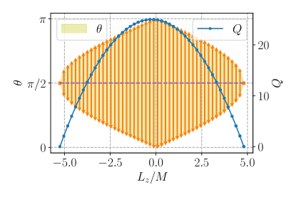
Figure 1: The range of the inclination angle $\theta$ (shaded area with arrows) and the value of the Carter constant $Q$ (blue curve with dots) as a function of $L_{z}$ , the angular-momentum component projected on the spin axis of the central Kerr SMBH. We have assumed $r_{p}=10M$ and $s=0.9$ in the plot.

2.3 Tidal forces in the free-fall frame

Having set up a parabolic orbit, we now calculate the tidal forces in the frame freely falling along the parabola. In this work we will focus on the GE forces. We can neglect the GM ones for the following two reasons. (i) The GM forces, according to Equation (2), are smaller than the GE ones by a factor of $v/c$. In our problem where $a\simeq(10^{3}-10^{4})m_{12}$, we have $v/c\sim{\cal O}(10^{-2})$. (ii) In our earlier work we found that the dynamical effect of GM forces is accumulative (Chen & Zhang, 2022). In order for such an effect to build up, the inner binary has to complete tens of revolutions. However, the parabolic encounter considered here is much quicker. Typically, the inner binary has time to complete only a couple of revolution during the pericenter passage.

Since GE forces are commonly known as the “tidal forces”, the corresponding Riemann tensor, i.e., $R_{ij}$ in Equation (3), are also called the tidal tensor. The tidal tensor in an FFF moving along an arbitrary time-like geodesic has been derived in Marck (1983). Its components are the simplest when written in a local inertia frame (LIF), which differs from the FFF by a rotation (see our earlier work, Chen & Zhang, 2022, for explanation). In the LIF, the $R_{13}$ and $R_{23}$ components and their symmetric parts (note that $R_{ij}$ is symmetric) will vanish.

While the tidal tensor of a circular outer orbit (the focus of our previous work) contains only diagonal components in the LIF and remains constant, the tidal tensor of a parabolic geodesic differs drastically. First, the off-diagonal component $R_{12}$ in the LIF will appear as soon as the geodesic leaves the equatorial plane of the SMBH. This property is illustrated in Figure 2, where the color map shows the magnitude of the tidal force, $R_{12}a$, divided by the self-gravity of the inner binary, $-m_{12}/a^{2}$. We can see that the $R_{12}$ component is non-zero outside the equatorial plane, and it can produce a tidal force as large as $40\%$ of the self-gravity of the inner BBH when $r$ approaches the pericenter. This tidal force is comparable to the ones resulting from the diagonal components of the tidal tensor (see the contours). Such a large off-diagonal component will impose an additional tidal torque which is absent from the earlier studies of the BBHs in the equatorial plane.

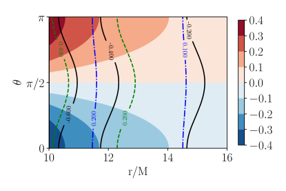
Figure 2: Tidal forces in the local inertia frame as a function of the Boyer-Lindquist coordinates $r$ and $\theta$. The color map shows the force induced by the off-diagonal component $R_{12}$ of the tidal tensor. In comparison, the black solid, green dashed, and blue dot-dashed contours correspond to the forces induced by, respectively, $R_{11}$, $R_{22}$, $R_{33}$. The value shown here is in unit of the self-gravity of the BBH, i.e., $-m_{12}/a^{2}$. In the plot, we have assumed $M=4\times 10^{6}M_{\odot}$, $m_{1}=15M_{\odot}$, $m_{2}=10M_{\odot}$, $a=2\times 10^{4}m_{12}$, $E=1$, $r_{p}=10M$, $s=0.9$, and $L_{z}=2.2M$.

The second dynamical effect induced by a parabolic orbit is a variation of the rotational velocity of the FFF relative to the LIF. This rotational velocity can be calculated with

$$\omega= \frac{K^{\frac{1}{2}}}{r^{2}+s^{2}M^{2}\cos^{2}\theta}$$ (7)

$$\times \left(\frac{r^{2}+s^{2}M^{2}-sML_{z}}{r^{2}+K}+\frac{sML_{z}-s^{2}M^{2}\sin^{2}\theta}{K-s^{2}M^{2}\cos^{2}\theta}\right)$$

(see Eq. (46) in Marck, 1983), where $K=(sME-L_{z})^{2}+Q$ is another definition of the Carter constant and we have used $E=1$ in the calculation. Figure 3 shows the value of $\omega$ for different $r$ and $\theta$. We find that the rotational velocity is determined mainly by the $r$ coordinate, and it can vary by orders of magnitude along a parabolic orbit. Since the axes of the LIF determine the orientation of the tidal tensor, a variation of the rotational velocity of the LIF will make the tidal forces in the FFF behave more irregularly.

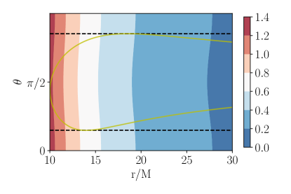
Figure 3: Rotational velocity of the tidal tensor in the FFF as a function of the $r$ and $\theta$ coordinates. The value is in unit of $\sqrt{M/r_{p}^{3}}$. The yellow curve shows the projection of a parabolic orbit, which starts in the equatorial plane at a radius of $r=100M$. The black dashed lines are the expected turning points in the $\theta$ direction. The other parameters are the same as in Figure 2.

3 Scattering experiments and results

3.1 Initial conditions

In our fiducial model, we choose the following parameters, $M=4\times 10^{6}M_{\odot}$, $s=0.9$, $m_{1}=15M_{\odot}$, and $m_{2}=10M_{\odot}$. The mass of the SMBH resembles that of the Milky Way, although it is unlikely that the SMBH in the Galactic Center is currently accompanied by a BBH (Chen & Han, 2018; Peng & Chen, 2021).

For the outer orbit, we assume that initially $r_{p}=10M$ and $E=1$. For $L_{z}$, we assume a uniform distribution within the range given by Equation (6). Such a distribution corresponds to a random distribution of orbital inclination with respect to the equatorial plane of the Kerr SMBH. Moreover, initially we place the c.m. of the BBH in the equatorial plane. It will later leave the equatorial plane if $Q>0$. Note that the above initial conditions cannot determine the initial radius of the outer orbit. For this reason, we choose $r_{\rm ini}=100M$. Such a radius is far enough from the central SMBH, so that the tidal perturbation has not significantly affected the dynamics of the BBH. Meanwhile, $r_{\rm ini}$ is relatively small, so that we can complete the simulation within a reasonable amount of computational time.

For the inner BBH, we choose an initial semimajor axis of $a_{0}=20,000m_{12}$, which corresponds to an orbital period of $\tau_{0}=2\pi\sqrt{a_{0}^{3}/m_{12}}\simeq 2,217~{}{\rm s}$. Since $a_{0}$ is much smaller than the curvature radius of the Kerr SMBH, the precision in the calculation of the GEM forces can be guaranteed. For simplicity, we further assume that the inner orbit is initially circular. The corresponding GW radiation timescale is $5a_{0}^{4}/(256m_{1}m_{2}m_{12})\simeq 52,000$ yrs (Peters, 1964), much longer than the mission duration of LISA. As for the stability of the BBH, we follow the convention and define a penetration factor of $\beta=r_{t}/r_{p}$, where $r_{t}=(M/m_{12})^{1/3}a_{0}$ is the tidal disruption radius derived in the Newtonian limit. In our fiducial model, we have $\beta\simeq 0.6786$, indicating that the BBH is marginally stable. The inclination of the inner BBH is defined by the angle $\iota$ between the inner orbital angular momentum of the BBH with respect to the rotating axis of the LIF.

3.2 Parameter space of the surviving BBHs

Since the penetration factor in our fiducial model is close to unity, a large fraction of the BBHs are tidally disrupted during their encounters with the central Kerr SMBH. Interesting, according to Figure 4, the surviving binaries occupy a specific region in the parameter space of $L_{z}$ and $\iota$.

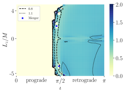
Figure 4: Dependence of the final semimajor axis of the inner BBH on the initial values of $L_{z}$ and $\iota$. The other parameters are the same as in Figure 2. The solid curve marks the boundary between tidal disruption and survival. The dashed and dotted contours show the regions where the final semimajor axis is, respectively, $0.8a_{0}$ and $1.1a_{0}$. The blue stars show the cases in which the BBHs coalesce during the pericenter passage.

The survivors reside mostly at $\iota\gtrsim\pi/2$. The reason for their survival is that they are counterrotating with respect to the LIF. For example, the rotational velocity of the BBH itself is about $\omega_{b}=\sqrt{m_{12}/a^{3}}\simeq 5.2\times 10^{-3}\rm{rad/s}$, and the rotational velocity of the LIF relative to the FFF is $\omega\sim\sqrt{M/r_{p}^{3}}\simeq 3\times 10^{-3}\rm{rad/s}$ when the BBH approaches the pericenter of the outer orbit. Therefore, in the rest frame of the binary, the tidal field could rotate at an angular velocity as high as $\omega_{b}+\omega\simeq 8\times 10^{-3}\rm{rad/s}$. Such a rapid variation effectively washes out the asymmetry of the tidal field, so that tidal disruption becomes less likely. In the following, we refer to these BBHs with $\iota>\pi/2$ as “retrograde” binaries. On the contrary, the BBHs with $\iota<\pi/2$ are rotating in the same sense as the rotation of the LIF, and we call them “prograde” binaries. In the rest frame of a prograde BBH, the LIF has an angular velocity of $\omega-\omega_{b}\simeq-2\times 10^{-3}\rm{rad/s}$. Such a slower rotation induces a more persistent tidal force on the BBH, so that the binary is disrupted more easily.

Figure 4 also shows that $L_{z}$ plays a minor role in determining the stability of the BBHs. The weak dependence reflects the fact that at $r=r_{p}$, the angular velocity of the LIF, $\omega$, is insensitive to the value of $L_{z}$. Nevertheless, close to $L_{z}\simeq 4M$ and $L_{z}\simeq-5M$, more BBHs are tidally disrupted than in the other cases of $L_{z}$. The reason is that the orbits here are closer to the equatorial plane when $|L_{z}|$ is greater. According to Figure 2, the tidal forces induced by the diagonal components of the tidal tensor are larger in the equatorial plane than in the polar regions.

We notice that Heggie & Rasio (1996) studied the interaction of a binary with a third body and derived a criterion for the survival of the binary,

$$\mathcal{F}^{-1}(\iota)>6\sqrt{\pi}2^{1/4}\beta^{-3/4}\exp\left[-\frac{2\sqrt{2}}{3}\beta^{-3/2}\right],$$ (8)

where $\mathcal{F}(\iota)=(\cos\iota+1)(\cos\iota+5)^{2}/72$. Recently, Addison et al. (2019) used the same criterion to identify surviving BBHs around SMBH. However, the criterion is derived using Newtonian forces. Its efficacy in the relativistic case is not yet testified.

Figure 5 compares the Newtonian criterion (red solid line) with the results derived in our relativistic simulations (lines with symbols as well as the blue shaded region). In the plot, the survivors are lying either above a demarcation line or in the shaded area, depending on their initial conditions. Interestingly, we find good agreement in most of the cases. Significant deviation appears when the penetration factor $\beta$ exceeds $0.9$, in the simulations of $s=0.9$ and $L_{z}<0$ (green line with down triangles). In these cases, we see that the BBH in the relativistic simulation is more stable than that in the Newtonian one. The stability in the relativistic simulation could be attributed to a faster rotation of the tidal field with respect to the rest frame of the BBH.

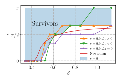
Figure 5: Comparing the Newtonian criterion (red solid line) for the survival of BBHs with the results of our relativistic simulations. The upper and down triangles refer to the simulations with an outer orbit inside the equatorial plane of a Kerr SMBH (with a spin parameter of $s=0.9$). The difference is that the upper triangles have $L_{z}>0$, while the lower triangles have $L_{z}<0$. The purple stars show the results of inclined orbits, which have $L_{z}=0$. The blue shaded region corresponds to the surviving BBHs around a Schwarzschild SMBH.

3.3 Eccentricities of the surviving BBHs

Beside semi-axis, the eccentricity of an inner BBH also varies during the interaction. Figure 6 shows the final eccentricity after the BBH has completed the interaction and traveled to a distance of $r=100M$ from the SMBH.

Figure 6: Final eccentricity of the inner binary as a function of the initial values of $L_{z}$ and $\iota$. The solid line marks the boundary between the surviving and the disrupted binaries. The dashed and the dotted lines show, respectively, the contours for $e_{\rm fin}=0.2$ and $e_{\rm fin}=0.5$. The other parameters are the same as in Figure 2.

First, we find that the final eccentricity $e_{\rm fin}$ can exceed $0.5$ when the inner BBH is inclined with respect to the rotational axis of the LIF, i.e., when $\iota\simeq\pi/2$. The cause is similar to the classical Von Zeipel-Lidov-Kozai mechanism, in which the inner binary trades its inclination for eccentricity (von Zeipel, 1910; Lidov, 1962; Kozai, 1962). The major difference, however, is that the tidal tensor in our LIF is asymmetric and contains non-diagonal terms, while in the classical scenario the tidal tensor is diagonal and is symmetric in the two azimuthal directions. Second, close to $L_{z}=0$, some BBHs with $\iota\neq\pi/2$ are also excited to high eccentricities. The cause, as has been shown in Figure 2, is the appearance of large off-diagonal terms in the tidal tensor as the binary reaches the polar regions of the Kerr SMBH. Third, we find that slightly more BBHs at $L_{z}<0$ than those at $L_{z}>0$ are excited to an eccentricity of $e_{\rm fin}>0.2$. The reason is that the rotation velocity $\omega$ of the LIF is slightly smaller when $L_{z}<0$. Therefore, in the rest frame of the BBH, the tidal field rotates slower, since this relative rotational velocity is $\omega+\omega_{b}$ for $\iota>\pi/2$.

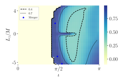
Figure 7: Same as Figure 4 but showing the maximum eccentricity of the inner BBH during the encounter with the Kerr SMBH.

We notice that during the close encounter with the central SMBH, a BBH can temporarily reach a very high eccentricity. Figure 7 shows the maximum eccentricity recorded during the interaction of each BBH with the SMBH. We find that most surviving BBHs have reached an eccentricity as high as $e_{\rm max}=0.4$, and many have exceeded $e_{\rm max}=0.7$. Such large eccentricities are expected to result in GW bursts, which will be further discussed in Section  4.1.

Significant variation of the eccentricity of the inner binary is also found in our earlier study of a BBH moving along a circular orbit in the equatorial plane (Chen & Zhang, 2022). However, it happens only when the binary is much closer to the SMBH, e.g., $r<3M$. In the current work, the closest distance between the BBH and the SMBH is $10M$. Nevertheless, significant variation of eccentricity is seen in a large fraction of the parameter space (see Figure 7). Such an easier excitation of eccentricity highlights the dynamical consequence of the asymmetric tidal tensors at the places outside the equatorial plane. It also indicates that BBHs reaching a distance of $r\sim 10M$ from a SMBH are more susceptible to merger than previously thought.

3.4 Lifetimes of the surviving BBHs

We have seen that the eccentricities of the surviving BBHs are excited during their close encounters with the Kerr SMBH. The lifetime of a compact binary is sensitive to the eccentricity since the GW radiation timescale is

$$T_{\mathrm{gw}} =\frac{5a^{4}F(e)}{256m_{1}m_{2}m_{12}}\simeq 5.2\times 10^{4}\left(\frac{a}{a_{0}}\right)^{4}F(e)~{}{\rm yr},$$ (9)

where $F(e)=(1-e_{0}^{2})^{7/2}(1+73/24e_{0}^{2}+37/96e_{0}^{4})^{-1}$ (Peters, 1964) and $a_{0}=20,000m_{12}$ is the initial semimajor axis. As a result, we expect a shorter lifetime for the surviving binaries.

The lifetimes of the post-interaction BBHs are shown in Figure 8, where we have assumed a random distribution for the initial orientation of the BBHs in the FFF. We find that in $54\%$ of the cases, the interaction results in a BBH with a shorter lifetime. Only in about $3\%$ of our simulations do we find a longer lifetime for the BBH after the interaction. Noticeably, in about $12\%$ ($4\%$) of the case, the lifetime is shortened by a factor of $10$ ($10^{4}$).

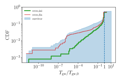
Figure 8: Cumulative distribution function of the ratios $T_{\rm gw}/T_{{\rm gw},0}$ for the BBHs surviving the interaction with the SMBH (blue histogram), where $T_{{\rm gw},0}\simeq 2\times 10^{5}~{}{\rm yrs}$ is the GW-radiation timescale of the original BBH and $T_{\rm gw}$ is the corresponding timescale after the interaction. The blue dashed vertical line marks the boundary of $T_{\rm gw}/T_{{\rm gw},0}=1$. The green thick (red thin) histogram corresponds to the BBHs which are initially (finally) counterrotating relative to the LIF.

The green thick (red thin) histogram in Figure 8 shows the BBHs which are counterrotating ($\iota>\pi/2$) with respect to the LIF before (after) the interaction with the SMBH. At $T_{\rm gw}/T_{{\rm gw},0}\lesssim 0.1$, we see a significant increase of the number of retrograde BBHs after the interaction has completed. This result indicates that many BBHs with significantly shortened lifetimes are originally corotating ($\iota<\pi/2$) with the LIF, but their orbital orientations flip during the interaction with the SMBH. Such an orbital flipping will affect the effective spin of the binaries (also noticed in Fernández & Kobayashi, 2019), which will be further discussed in section 4.2.

In particular, in about $f_{m}\simeq 0.17\%$ of our scattering experiments, we find that the BBHs coalesce during the encounter with the SMBH. In another $f_{i}\simeq 24.1\%$ of the cases, the lifetimes of the BBHs are shortened to a value significantly less than the typical dynamical timescale of the galactic nucleus, $r_{i}/\sigma\simeq 4\times 10^{4}$ yrs, where $\sigma\simeq 75~{}\mathrm{kms^{-1}}$ is the stellar velocity dispersion of the nucleus of a Milky-Way-like galaxy (Tremaine et al., 2002) and $r_{i}=GM/\sigma^{2}$ is the radius of gravitational influence of the SMBH. The latter BBHs, because of their shortened lifetimes, will also coalesce before they come back to interact with the SMBH again. Taking the above two types of binaries into account, we derive a lower limit for the merger rate of BBHs,

$$\mathcal{R} =p\Gamma_{\mathrm{BHB}}\cdot n_{g}\cdot f$$ (10)

$$\simeq(0.78-1.94)\times 10^{-2}\mathrm{Gpc^{-3}yr^{-1}},$$

where $p\Gamma_{\mathrm{BHB}}\sim(1.6-4)\times 10^{-9}~{}\mathrm{yr}^{-1}~{}\mathrm{galaxy}^{-1}$ is the supply rate of compact BBHs ($a\sim a_{0}$) to the SMBH which was estimated in Han & Chen (2019), $n_{g}\sim 2\times 10^{7}~{}\mathrm{Gpc}^{-3}$ is the number density of galaxies (Conselice et al., 2005), and $f=(f_{i}+f_{m})\simeq 0.24$. The real merger rate should be higher since many surviving BBHs could come back and interact with the SMBH again. A more accurate estimation of the merger rate requires a dynamical model which can self-consistently track the formation and evolution of BBHs in nuclear star clusters (e.g. Zhang & Amaro Seoane, 2023). We will incorporate such a model in our future work.

4 Discussions and conclusion

In this work, we simulated the close encounter ($r_{p}=10M$) of a Kerr SMBH with a BBH coming from a parabolic outer orbit. We solved the equations of motion of the binary in its FFF, in which the dynamics is no longer highly relativistic. We showed that in the FFF, a BBH rotating in the same direction as the tidal field is more likely disrupted. Those surviving binaries, mostly counterrotating with respect to the tidal field, are excited by the tidal field to a large orbital eccentricity so that about $54\%$ of them end up with a shorter lifetime. Our results have important implications for future GW observations, which we now discuss.

4.1 Multi-band GW bursts

The reason why we consider $a_{0}\sim 10^{4}m_{12}$ is that such a binary falls in the sensitive band of LISA (also see Chen & Han, 2018; Chen & Zhang, 2022). The frequency of the GWs is

$$f_{\mathrm{gw}}\sim 2f_{\mathrm{orb}} =\frac{1}{\pi}\sqrt{\frac{m_{12}}{a^{3}}}$$ (11)

$$=0.23\mathrm{mHz}\left(\frac{m_{12}}{\mathrm{25}M_{\odot}}\right)^{-1}\left(\frac{a}{a_{0}}\right)^{-3/2},$$

where we have assumed $e=0$. The amplitude of the GW radiation is

$$h_{\mathrm{gw}} \sim\sqrt{\frac{32}{5}}\frac{m_{1}m_{2}}{d\,a}$$ (12)

$$\simeq 3.6\times 10^{-21}\left(\frac{d}{\mathrm{10kpc}}\right)^{-1}\left(\frac{a}{a_{0}}\right)^{-1}$$

(Peters & Mathews, 1963; Xuan et al., 2023), where $d$ is the luminosity distance of the source. The latter equation indicates that under normal circumstances it is difficult for LISA to catch such a BBH unless the binary is inside the Milky Way.

However, the increase of the inner orbital eccentricity during the encounter with the SMBH, as is shown in Figure 7, could shift the main power of the GW radiation into the LIGO/Virgo band. It is known that the frequency where the GW spectrum peaks correlates with the characteristic frequency of the orbital pericenter, $\sqrt{m_{12}/r_{p,b}^{3}}/\pi$, where $r_{p,b}$ is the pericenter distance of the inner orbit (Wen, 2003). In our simulations, we found that $r_{p,b}$ could be as small as $0.002a_{0}$ in about $0.3\%$ of the cases. Therefore, the GW frequency could increase to

$$f_{\mathrm{{gw},p}}\simeq 2.52\mathrm{Hz}\left(\frac{m_{12}}{\mathrm{25}M_{\odot}}\right)^{-1}\left(\frac{r_{p,b}}{0.002a_{0}}\right)^{-3/2},$$ (13)

a frequency to which LIGO/Virgo are sensitive. Moreover, the GW amplitude of an eccentric BBH can be estimated with

$$h_{\mathrm{gw},p}\simeq 1.8\times 10^{-22}\left(\frac{d}{\mathrm{100Mpc}}\right)^{-1}\left(\frac{r_{p,b}}{0.002a_{0}}\right)^{-1}$$ (14)

(Xuan et al., 2023). Such an amplitude becomes accessible by the current LIGO/Virgo detectors.

Therefore, even though we started with a LISA BBH, the binary could exit the LISA band and enter the LIGO/Virgo band during its closer encounter with the central SMBH. Note that the encounter is short, lasting only a couple of orbital periods of the BBH, since $\omega_{b}/\omega$ is slightly greater than unity. After the encounter, the eccentricity of the BBH returns to a relatively low value as is shown in Figures 6, which indicates that the binary returns to the LISA band again. Such an excursion would have produced a couple of detectable bursts in the LIGO/Virgo band.

We have seen that when the inner binary enters the LIGO/Virgo band, the c.m. of the binary also reaches the pericenter of the outer orbit. This passage also produces a burst of GW radiation, which we refer to as the “extreme-mass-ratio burst” (EMRB). Notice that the conventional picture of an EMRB involves only one stellar-mass BH around an SMBH (Rubbo et al., 2006; Hopman et al., 2007; Yunes et al., 2008; Berry & Gair, 2013), but in our case we have two stellar-mass BHs (Fernández & Kobayashi, 2019). Following the earlier calculation of the GW signal of an eccentric binary, we find that the EMRB has a characteristic frequency of

$$f_{\mathrm{{EMRB}}}\simeq 0.13\mathrm{mHz}\left(\frac{M}{4\times 10^{6}M_{\odot}}\right)^{-1}\left(\frac{r_{p}}{10M}\right)^{-3/2},$$ (15)

and a typical amplitude of

$$h_{\mathrm{EMRB}}\simeq 3.1\times 10^{-21}\left(\frac{d}{\mathrm{100Mpc}}\right)^{-1}\left(\frac{r_{p}}{10M}\right)^{-1}.$$ (16)

Such a signal is detectable by LISA.

The above analysis of the GW signal indicates that our system may be a multi-band GW source. When the inner BBH passes by the central Kerr SMBH, its inner orbital eccentricity could be excited so that the binary produces high-frequency GW bursts which are detectable by LIGO/Virgo. Meanwhile, its motion around the SMBH could also produce a low-frequency GW burst which falls in the LISA band. Our analysis suggests that LIGO/Virgo/LISA can detect such a source out to a luminosity distance of ${\cal O}(10^{2})$ Mpc.

4.2 Effective spin of merging BBH

The effective spin of a BBH is a measurable quantity in GW signal (e.g. LIGO Scientific Collaboration & Virgo Collaboration, 2016), and it is defined as

$$\chi_{\mathrm{eff}}:= \frac{m_{1}\mathbf{S_{1}}+m_{2}\mathbf{S_{2}}}{m_{12}}\cdot\mathbf{\hat{L}_{in}},$$ (17)

where $\mathbf{S}_{1,2}$ are the dimensionless spin vectors of the two BHs, and $\mathbf{\hat{L}_{in}}$ is a unit vector aligned with the orbital angular momentum of the BBH (Damour, 2001; Santamaría et al., 2010; Ajith et al., 2011). It is suggested that the distribution of $\chi_{\mathrm{eff}}$ could reveal the formation channel of the LIGO/Virgo BBHs (Farr et al., 2017; Talbot & Thrane, 2017; Vitale et al., 2017). We have seen in Section 3.4 that the orbital angular momentum of a BBH could flip its direction during the close interaction of the binary with the SMBH. According to Equation (17), the value of $\chi_{\mathrm{eff}}$ will change.

To understand the impact of the angular-momentum flip on observation, here we analyze the distribution of $\chi_{\mathrm{eff}}$ during two phases when the GW is the strongest, i.e., (i) the burst phase when the eccentricity of a BBH is the highest and (ii) the final merger when the BBH is safely in the LIGO/Virgo band. To simplify the analysis, we assume that initially the spin axes are aligned with the original direction of the angular momentum, $\mathbf{\hat{L}_{in,0}}$, so that $\chi_{\mathrm{eff},0}/S=1$. We also assume that during the interaction the direction and magnitude of the spin of each BH is constant (in the FFF), since the term of spin-orbit coupling is only a factor of $(v/c)^{3/2}/0.1\sim{\cal O}(10^{-2})$ of the tidal force imposed on the BBH. Therefore, the effective spin during the encounter with the SMBH can be calculated with

$$\chi_{\mathrm{eff}}/S=\mathbf{\hat{L}_{in,0}}\cdot\mathbf{\hat{L}_{in}},$$ (18)

where $S=(m_{1}|\mathbf{S}_{1}|+m_{2}|\mathbf{S}_{1,2}|)/m_{12}$ is the dimensionless spin of the BBH. After the encounter ($r>100M$), $\chi_{\mathrm{eff}}$ remains approximately constant (Racine, 2008).

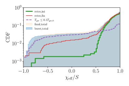
Figure 9: Cumulative probability distribution of the effective spins of the inner binaries. The yellow and blue histograms show the effective spins measured at, respectively, the final merger and the burst phase. The green and red histograms have the same meanings as in Fig. 8 but for the effective spins of the merging BBHs. Additionally, the purple dashed histogram shows the distribution of the BBHs whose lifetimes are shortened by more than a factor of $10$ due to their interaction with the SMBH.

The cumulative distribution of $\chi_{\mathrm{eff}}/S$ is shown in Figure 9. We find that during the burst phase and the final merger, the effect spin covers a wide range, unlike its initial distribution only at $\chi_{\mathrm{eff}}/S=1$. About $4\%$ of the surviving BBHs have $\chi_{\rm eff}\leq-0.5$ when they merge. This fraction is about four times higher than the percentage found previously in Newtonian simulations (see Fig. (7) in Fernández & Kobayashi, 2019). The significant difference highlights the necessity of carrying out relativistic three-body simulations like ours.

Figure 9 also shows that at $\chi_{\rm eff}\leq 0.5$, a relatively small fraction of BBHs initially have retrograde inner orbits. This result corroborates our earlier observations that retrograde inner binaries in general are more stable than those prograde ones.

4.3 Caveats

So far, we have focused on the systems with parabolic outer orbits. However, our method also applies to the BBHs on eccentric or hyperbolic outer orbits. In particular, BBHs moving on eccentric outer orbits could be produced by a dynamical process called “tidal capture” (Chen & Han, 2018; Addison et al., 2019). Such a captured BBH would interact with the central SMBH multiple times before it is either tidally disrupted or driven to merger. To study the final outcome, we need to further consider the cumulative loss of the energy and angular momentum of the outer orbit during successive close encounters.

When choosing the initial conditions, we only considered a variation of the orientations of the inner and outer orbits while keeping the other parameters fixed. It has been reported by previous works that the initial values of the ascending node and the phase of the inner binary also play a important role in determining the outcome (Addison et al., 2019; Fernández & Kobayashi, 2019). Dedicated simulations are needed to cover such a parameter space of higher dimension.

When estimating the frequency and amplitude of the GW burst emitted during a close encounter of two BHs, we made a simplification that the observable quantities are similar to those of a circular binary whose orbital semimajor axis is the same as the closest distance during the encounter. However, a burst signal contains multiple GW frequencies and, in fact, we have considered in this work only the most powerful GW mode. Taking the full GW spectrum into account could enhance the signal-to-noise ratio and help identify burst events in future GW observations.

Although the PN formalism adopted in this work can appropriately treat the evolution of the BH spin in the FFF, we find that in most cases the corresponding term (1.5 PN) remains small relative to the GE force. This is the reason why we only considered the variation of the orbital angular momentum when we calculated the effective spin of the inner binary. Only in a couple of rare cases, where the BBHs coalesce during their close encounter with the SMBH, did we find that the 1.5PN term is no longer negligible. In these cases, the BHs become so close to each other that higher order PN corrections, such as those up to 3.5 PN order (Will, 2017), need to be included in the calculation.

Despite these caveats, our series of works (also see Chen & Zhang, 2022) have established a framework which can simulate the dynamical evolution of a compact binary moving on an arbitrary orbit around a Kerr SMBH. Further improvements, as described above, will enable us to derive long-term evolution of the triple system and construct accurate waveforms, which are very much needed for the detection such sources in GW observation.

5 Acknowledgement

This work is supported by the National Key Research and Development Program of China Grant No. 2021YFC2203002 and the National Natural Science Foundation of China (NSFC) grant No. 11991053.

References

- Addison et al. (2019) Addison, E., Gracia-Linares, M., Laguna, P., & Larson, S. L. 2019, General Relativity and Gravitation, 51, 38, doi: 10.1007/s10714-019-2523-4
- Ajith et al. (2011) Ajith, P., Hannam, M., Husa, S., et al. 2011, Phys. Rev. Lett., 106, 241101, doi: 10.1103/PhysRevLett.106.241101
- Amaro-Seoane et al. (2023) Amaro-Seoane, P., Andrews, J., Arca Sedda, M., et al. 2023, Living Reviews in Relativity, 26, 2, doi: 10.1007/s41114-022-00041-y
- Antonini et al. (2010) Antonini, F., Faber, J., Gualandris, A., & Merritt, D. 2010, ApJ, 713, 90, doi: 10.1088/0004-637X/713/1/90
- Antonini & Perets (2012) Antonini, F., & Perets, H. B. 2012, ApJ, 757, 27, doi: 10.1088/0004-637X/757/1/27
- Arca Sedda (2020) Arca Sedda, M. 2020, ApJ, 891, 47, doi: 10.3847/1538-4357/ab723b
- Bai et al. (2011) Bai, S., Cao, Z., Han, W.-B., et al. 2011, in Journal of Physics Conference Series, Vol. 330, Journal of Physics Conference Series, 012016, doi: 10.1088/1742-6596/330/1/012016
- Bardeen et al. (1972) Bardeen, J. M., Press, W. H., & Teukolsky, S. A. 1972, ApJ, 178, 347, doi: 10.1086/151796
- Bartos et al. (2017) Bartos, I., Kocsis, B., Haiman, Z., & Márka, S. 2017, ApJ, 835, 165, doi: 10.3847/1538-4357/835/2/165
- Baruteau et al. (2011) Baruteau, C., Cuadra, J., & Lin, D. N. C. 2011, ApJ, 726, 28, doi: 10.1088/0004-637X/726/1/28
- Bellovary et al. (2016) Bellovary, J. M., Mac Low, M.-M., McKernan, B., & Ford, K. E. S. 2016, ApJ, 819, L17, doi: 10.3847/2041-8205/819/2/L17
- Berry & Gair (2013) Berry, C. P. L., & Gair, J. R. 2013, 429, 589, doi: 10.1093/mnras/sts360
- Blanchet (2014) Blanchet, L. 2014, Living Reviews in Relativity, 17, 2, doi: 10.12942/lrr-2014-2
- Bonvin et al. (2017) Bonvin, C., Caprini, C., Sturani, R., & Tamanini, N. 2017, Phys. Rev. D, 95, 044029, doi: 10.1103/PhysRevD.95.044029
- Camilloni et al. (2023) Camilloni, F., Grignani, G., Harmark, T., et al. 2023, Phys. Rev. D, 107, 084011, doi: 10.1103/PhysRevD.107.084011
- Campbell & Matzner (1973) Campbell, G. A., & Matzner, R. A. 1973, Journal of Mathematical Physics, 14, 1, doi: 10.1063/1.1666159
- Cardoso et al. (2021) Cardoso, V., Duque, F., & Khanna, G. 2021, Phys. Rev. D, 103, L081501, doi: 10.1103/PhysRevD.103.L081501
- Carter (1968) Carter, B. 1968, Phys. Rev., 174, 1559, doi: 10.1103/PhysRev.174.1559
- Chen & Han (2018) Chen, X., & Han, W.-B. 2018, Communications Physics, 1, 53, doi: 10.1038/s42005-018-0053-0
- Chen et al. (2019) Chen, X., Li, S., & Cao, Z. 2019, Monthly Notices of the Royal Astronomical Society: Letters, 485, L141, doi: 10.1093/mnrasl/slz046
- Chen & Zhang (2022) Chen, X., & Zhang, Z. 2022, Phys. Rev. D, 106, 103040, doi: 10.1103/PhysRevD.106.103040
- Cheng & Wang (1999) Cheng, K. S., & Wang, J.-M. 1999, ApJ, 521, 502, doi: 10.1086/307572
- Conselice et al. (2005) Conselice, C. J., Blackburne, J. A., & Papovich, C. 2005, ApJ, 620, 564, doi: 10.1086/426102
- Damour (2001) Damour, T. 2001, Phys. Rev. D, 64, 124013, doi: 10.1103/PhysRevD.64.124013
- DeLaurentiis et al. (2023) DeLaurentiis, S., Epstein-Martin, M., & Haiman, Z. 2023, MNRAS, 523, 1126, doi: 10.1093/mnras/stad1412
- D’Orazio & Loeb (2020) D’Orazio, D. J., & Loeb, A. 2020, Phys. Rev. D, 101, 083031, doi: 10.1103/PhysRevD.101.083031
- Fang et al. (2019) Fang, Y., Chen, X., & Huang, Q.-G. 2019, ApJ, 887, 210, doi: 10.3847/1538-4357/ab510e
- Farr et al. (2017) Farr, W. M., Stevenson, S., Miller, M. C., et al. 2017, Nature, 548, 426, doi: 10.1038/nature23453
- Fermi (1922) Fermi, E. 1922, Rend. Lincei, 31, 21
- Fernández & Kobayashi (2019) Fernández, J. J., & Kobayashi, S. 2019, MNRAS, 487, 1200, doi: 10.1093/mnras/stz1353
- Fragione et al. (2019) Fragione, G., Grishin, E., Leigh, N. W. C., Perets, H. B., & Perna, R. 2019, MNRAS, 488, 47, doi: 10.1093/mnras/stz1651
- Gondán & Kocsis (2022) Gondán, L., & Kocsis, B. 2022, MNRAS, 515, 3299, doi: 10.1093/mnras/stac1985
- Gong et al. (2021) Gong, Y., Cao, Z., & Chen, X. 2021, Phys. Rev. D, 103, 124044, doi: 10.1103/PhysRevD.103.124044
- Gorbatsievich & Bobrik (2010) Gorbatsievich, A., & Bobrik, A. 2010, AIP Conference Proceedings, 1205, 87, doi: 10.1063/1.3382338
- Hamers et al. (2018) Hamers, A. S., Bar-Or, B., Petrovich, C., & Antonini, F. 2018, ApJ, 865, 2, doi: 10.3847/1538-4357/aadae2
- Han & Chen (2019) Han, W.-B., & Chen, X. 2019, MNRAS, 485, L29, doi: 10.1093/mnrasl/slz021
- Heggie & Rasio (1996) Heggie, D. C., & Rasio, F. A. 1996, MNRAS, 282, 1064, doi: 10.1093/mnras/282.3.1064
- Hills (1988) Hills, J. G. 1988, 331, 687
- Hills (1991) —. 1991, 102, 704
- Hoang et al. (2018) Hoang, B.-M., Naoz, S., Kocsis, B., Rasio, F. A., & Dosopoulou, F. 2018, ApJ, 856, 140, doi: 10.3847/1538-4357/aaafce
- Hopman et al. (2007) Hopman, C., Freitag, M., & Larson, S. L. 2007, 378, 129, doi: 10.1111/j.1365-2966.2007.11758.x
- Inayoshi et al. (2017) Inayoshi, K., Tamanini, N., Caprini, C., & Haiman, Z. 2017, Phys. Rev. D, 96, 063014, doi: 10.1103/PhysRevD.96.063014
- Kocsis (2013) Kocsis, B. 2013, ApJ, 763, 122, doi: 10.1088/0004-637X/763/2/122
- Komarov et al. (2018) Komarov, S., Gorbatsievich, A., & Tarasenko, A. 2018, General Relativity and Gravitation, 50, 132, doi: 10.1007/s10714-018-2461-6
- Kozai (1962) Kozai, Y. 1962, AJ, 67, 591, doi: 10.1086/108790
- Kuntz et al. (2021) Kuntz, A., Serra, F., & Trincherini, E. 2021, Phys. Rev. D, 104, 024016, doi: 10.1103/PhysRevD.104.024016
- Kuntz et al. (2023) —. 2023, Phys. Rev. D, 107, 044011, doi: 10.1103/PhysRevD.107.044011
- Lawrence (1973) Lawrence, J. K. 1973, Phys. Rev. D, 7, 2275, doi: 10.1103/PhysRevD.7.2275
- Li et al. (2023) Li, J., Dempsey, A. M., Li, H., Lai, D., & Li, S. 2023, ApJ, 944, L42, doi: 10.3847/2041-8213/acb934
- Li et al. (2022) Li, J., Lai, D., & Rodet, L. 2022, ApJ, 934, 154, doi: 10.3847/1538-4357/ac7c0d
- Lidov (1962) Lidov, M. L. 1962, Planet. Space Sci., 9, 719, doi: 10.1016/0032-0633(62)90129-0
- Ligo Scientific Collaboration et al. (2023) Ligo Scientific Collaboration, Collaboration, V., & Kagra Collaboration. 2023, Physical Review X, 13, 041039, doi: 10.1103/PhysRevX.13.041039
- LIGO Scientific Collaboration & Virgo Collaboration (2016) LIGO Scientific Collaboration, & Virgo Collaboration. 2016, Phys. Rev. Lett., 116, 241102, doi: 10.1103/PhysRevLett.116.241102
- Liu & Lai (2020) Liu, B., & Lai, D. 2020, Phys. Rev. D, 102, 023020, doi: 10.1103/PhysRevD.102.023020
- Liu & Lai (2022) —. 2022, ApJ, 924, 127, doi: 10.3847/1538-4357/ac3aef
- Liu et al. (2019) Liu, B., Lai, D., & Wang, Y.-H. 2019, ApJ, 883, L7, doi: 10.3847/2041-8213/ab40c0
- Maeda et al. (2023a) Maeda, K.-i., Gupta, P., & Okawa, H. 2023a, Phys. Rev. D, 107, 124039, doi: 10.1103/PhysRevD.107.124039
- Maeda et al. (2023b) —. 2023b, arXiv e-prints, arXiv:2309.12096, doi: 10.48550/arXiv.2309.12096
- Manasse & Misner (1963) Manasse, F. K., & Misner, C. W. 1963, Journal of Mathematical Physics, 4, 735, doi: 10.1063/1.1724316
- Marck (1983) Marck, J. A. 1983, Proceedings of the Royal Society of London Series A, 385, 431, doi: 10.1098/rspa.1983.0021
- Mashhoon (2003) Mashhoon, B. 2003, arXiv e-prints, gr. https://arxiv.org/abs/gr-qc/0311030
- McKernan et al. (2012) McKernan, B., Ford, K. E. S., Lyra, W., & Perets, H. B. 2012, MNRAS, 425, 460, doi: 10.1111/j.1365-2966.2012.21486.x
- Meiron et al. (2017) Meiron, Y., Kocsis, B., & Loeb, A. 2017, ApJ, 834, 200, doi: 10.3847/1538-4357/834/2/200
- Miller et al. (2005) Miller, M. C., Freitag, M., Hamilton, D. P., & Lauburg, V. M. 2005, 631, L117, doi: 10.1086/497335
- Oancea et al. (2022) Oancea, M. A., Stiskalek, R., & Zumalacárregui, M. 2022, arXiv e-prints, arXiv:2209.06459, doi: 10.48550/arXiv.2209.06459
- Ohanian (1973) Ohanian, H. C. 1973, Phys. Rev. D, 8, 2734, doi: 10.1103/PhysRevD.8.2734
- Peng & Chen (2021) Peng, P., & Chen, X. 2021, MNRAS, 505, 1324, doi: 10.1093/mnras/stab1419
- Peng & Chen (2023) —. 2023, ApJ, 950, 3, doi: 10.3847/1538-4357/acce3b
- Peters (1964) Peters, P. 1964, Physical Review (U.S.) Superseded in part by Phys. Rev. A, Phys. Rev. B: Solid State, Phys. Rev. C, and Phys. Rev. D, 136, doi: 10.1103/PhysRev.136.B1224
- Peters & Mathews (1963) Peters, P., & Mathews, J. 1963, Physical Review (U.S.) Superseded in part by Phys. Rev. A, Phys. Rev. B: Solid State, Phys. Rev. C, and Phys. Rev. D, 131, doi: 10.1103/PhysRev.131.435
- Petrovich & Antonini (2017) Petrovich, C., & Antonini, F. 2017, ApJ, 846, 146, doi: 10.3847/1538-4357/aa8628
- Racine (2008) Racine, E. 2008, Phys. Rev. D, 78, 044021, doi: 10.1103/PhysRevD.78.044021
- Rubbo et al. (2006) Rubbo, L. J., Holley-Bockelmann, K., & Finn, L. S. 2006, ApJ, 649, L25, doi: 10.1086/508326
- Santamaría et al. (2010) Santamaría, L., Ohme, F., Ajith, P., et al. 2010, Phys. Rev. D, 82, 064016, doi: 10.1103/PhysRevD.82.064016
- Secunda et al. (2019) Secunda, A., Bellovary, J., Mac Low, M.-M., et al. 2019, ApJ, 878, 85, doi: 10.3847/1538-4357/ab20ca
- Stone et al. (2017) Stone, N. C., Metzger, B. D., & Haiman, Z. 2017, MNRAS, 464, 946, doi: 10.1093/mnras/stw2260
- Tagawa et al. (2020) Tagawa, H., Haiman, Z., Bartos, I., & Kocsis, B. 2020, ApJ, 899, 26, doi: 10.3847/1538-4357/aba2cc
- Takátsy et al. (2019) Takátsy, J., Bécsy, B., & Raffai, P. 2019, MNRAS, 486, 570, doi: 10.1093/mnras/stz820
- Talbot & Thrane (2017) Talbot, C., & Thrane, E. 2017, Phys. Rev. D, 96, 023012, doi: 10.1103/PhysRevD.96.023012
- Tamanini et al. (2020) Tamanini, N., Klein, A., Bonvin, C., Barausse, E., & Caprini, C. 2020, Phys. Rev. D, 101, 063002, doi: 10.1103/PhysRevD.101.063002
- The LIGO Scientific Collaboration & the Virgo Collaboration (2019) The LIGO Scientific Collaboration, & the Virgo Collaboration. 2019, Physical Review X, 9, 031040, doi: 10.1103/PhysRevX.9.031040
- The LIGO Scientific Collaboration & the Virgo Collaboration (2020) —. 2020, arXiv e-prints, arXiv:2010.14527. https://arxiv.org/abs/2010.14527
- Torres-Orjuela & Chen (2023) Torres-Orjuela, A., & Chen, X. 2023, Phys. Rev. D, 107, 043027, doi: 10.1103/PhysRevD.107.043027
- Torres-Orjuela et al. (2020) Torres-Orjuela, A., Chen, X., & Amaro-Seoane, P. 2020, Ph. Rv. D, 101, 083028, doi: 10.1103/PhysRevD.101.083028
- Torres-Orjuela et al. (2019) Torres-Orjuela, A., Chen, X., Cao, Z., Amaro-Seoane, P., & Peng, P. 2019, Phys. Rev. D, 100, 063012, doi: 10.1103/PhysRevD.100.063012
- Tremaine et al. (2002) Tremaine, S., Gebhardt, K., Bender, R., et al. 2002, 574, 740
- Vijaykumar et al. (2022) Vijaykumar, A., Kapadia, S. J., & Ajith, P. 2022, MNRAS, doi: 10.1093/mnras/stac1131
- Vijaykumar et al. (2023) Vijaykumar, A., Tiwari, A., Kapadia, S. J., Arun, K. G., & Ajith, P. 2023, ApJ, 954, 105, doi: 10.3847/1538-4357/acd77d
- Vitale et al. (2017) Vitale, S., Lynch, R., Sturani, R., & Graff, P. 2017, Classical and Quantum Gravity, 34, 03LT01, doi: 10.1088/1361-6382/aa552e
- von Zeipel (1910) von Zeipel, H. 1910, Astronomische Nachrichten, 183, 345, doi: 10.1002/asna.19091832202
- Wang et al. (2019) Wang, Y.-H., Leigh, N. W. C., Sesana, A., & Perna, R. 2019, MNRAS, 490, 2627, doi: 10.1093/mnras/stz2780
- Wen (2003) Wen, L. 2003, ApJ, 598, 419, doi: 10.1086/378794
- Will (2014) Will, C. M. 2014, Phys. Rev. D, 89, 044043, doi: 10.1103/PhysRevD.89.044043
- Will (2017) —. 2017, Phys. Rev. D, 96, 023017, doi: 10.1103/PhysRevD.96.023017
- Xuan et al. (2023) Xuan, Z., Naoz, S., Kocsis, B., & Michaely, E. 2023, arXiv e-prints, arXiv:2310.00042, doi: 10.48550/arXiv.2310.00042
- Yan et al. (2023) Yan, H., Chen, X., & Torres-Orjuela, A. 2023, Phys. Rev. D, 107, 103044, doi: 10.1103/PhysRevD.107.103044
- Yu et al. (2021) Yu, H., Wang, Y., Seymour, B., & Chen, Y. 2021, Phys. Rev. D, 104, 103011, doi: 10.1103/PhysRevD.104.103011
- Yunes et al. (2008) Yunes, N., Sopuerta, C. F., Rubbo, L. J., & Holley-Bockelmann, K. 2008, 675, 604, doi: 10.1086/525839
- Zhang & Amaro Seoane (2023) Zhang, F., & Amaro Seoane, P. 2023, arXiv e-prints, arXiv:2306.03924, doi: 10.48550/arXiv.2306.03924
- Zhang et al. (2019) Zhang, F., Shao, L., & Zhu, W. 2019, ApJ, 877, 87, doi: 10.3847/1538-4357/ab1b28
- Zhang & Chen (2023) Zhang, X., & Chen, X. 2023, MNRAS, 521, 2919, doi: 10.1093/mnras/stad728