One Graph Model for Cross-domain Dynamic Link Prediction

Abstract

This work proposes DyExpert, a dynamic graph model for cross-domain link prediction. It can explicitly model historical evolving processes to learn the evolution pattern of a specific downstream graph and subsequently make pattern-specific link predictions. DyExpert adopts a decode-only transformer and is capable of efficiently parallel training and inference by conditioned link generation that integrates both evolution modeling and link prediction. DyExpert is trained by extensive dynamic graphs across diverse domains, comprising 6M dynamic edges. Extensive experiments on eight untrained graphs demonstrate that DyExpert achieves state-of-the-art performance in cross-domain link prediction. Compared to the advanced baseline under the same setting, DyExpert achieves an average of 11.40% improvement (Average Precision) across eight graphs. More impressive, it surpasses the fully supervised performance of 8 advanced baselines on 6 untrained graphs.

1 Introduction

Recently, building artificial intelligence (AI) systems for various downstream tasks has become a popular paradigm (Brown et al., 2020; Radford et al., 2021). These systems are usually based on “foundation models” (Bommasani et al., 2021), which are trained on broad and diverse datasets and can be broadly and conveniently adapted across a wide range of downstream tasks. Foundation models have gained significant success in various fields. For example, in the computer vision field, (Kirillov et al., 2023) has established the image segmentation model that achieves competitive zero-shot performance via large-scale training. Numerous successful cases demonstrate that foundation models offer several advantages over fully supervised models. Training on board datasets allows foundation models to scale up to larger parameters and achieve stronger expressiveness (Kaplan et al., 2020; Hoffmann et al., 2022). Then once foundation models are trained, they can conveniently provide services for broad masses and various applications.

In dynamic graph research (Zaki et al., 2016), link prediction holds significant potential to build foundation models. Various real-world scenarios, involving numerous entities engage in continuous interactions over time (Chakrabarti, 2007). These scenarios can be represented by dynamic graphs where nodes represent entities and edges denote their interactions at a timestamp (Kumar et al., 2019). Therefore, link prediction on dynamic graphs is an essential and all-inclusive task for numerous interaction-related applications, such as user-item recommendations (Ye et al., 2021). Each application can be framed as link predictions on graphs within a specific domain. Consequently, a model capable of cross-domain link prediction can bring benefits to numerous interaction-related applications across various scenarios.

This work aims to explore such a foundation model capable of cross-domain link prediction on dynamic graphs. The process of link prediction on a particular dynamic graph essentially involves learning the evolution patterns of the graph from previous links and extending the learned patterns to predict future edges, which can be generalized across domains instinctively. Graphs from different domains may share some similar evolution patterns, which we term “evolution similarities”. For instance, the triadic closure process (Zhou et al., 2018; Huang et al., 2014) is a similar evolution mechanism found in both friendships at a university (Kossinets & Watts, 2006) and scientific collaborations (Newman, 2001). Acquiring numerous such evolution patterns from extensive datasets and leveraging their similarities for cross-domain generalization is a promising way of building foundational models for dynamic link prediction.

Currently, dynamic graph models based on end-to-end learning achieve the advanced performance of dynamic link prediction in single-graph scenarios (Huang et al., 2023). Specifically, given a pair of nodes at a certain timestamp, these methods initially represent their previous temporal structures and then leverage their representations to predict the possibility of whether an edge exists between them in the future (Yu et al., 2023). For instance, TGAT (Xu et al., 2020) incorporates time encoders into Graph Neural Networks (GNNs) (Hamilton et al., 2017; Veličković et al., 2017) to effectively learn nodes’ temporal representation. These methods are trained by supervised learning (end2end) on historical edges from a specific graph (Wang et al., 2021b; Cong et al., 2023).

However, these methods have limitations in constructing foundational models, as diverse graphs encompass various physical meanings in cross-domain scenarios. For instance, two pairs from different graphs that share similar evolution patterns may have a significant gap between their structural representations, since they employ distinct metrics for recording time (Huang et al., 2023; Yu et al., 2023). In these scenarios, existing models encounter challenging limitations in the: (1) Learning evolution similarities. Current models lack awareness of the distinctions in the physical meaning of input graphs, thereby encountering difficulties in extracting similarities from cross-domain graphs. (2) Generalizing to other graphs. When faced with two pairs displaying comparable structures but stemming from graphs with entirely different physical meanings, these models still solely learn on nodes’ structure and give similar prediction results. Such a phenomenon may jeopardize the model’s effectiveness in cross-domain prediction.

Thus, we propose DyExpert, a cross-domain foundation model that explicitly models the evolution process of graphs and simultaneously performs evolution-specific link predictions. It adopts a decode-only transformer, enabling large-scale parallel training and efficient inference, and optimized by conditioned link generation (CLG) that can integrate the modeling of the evolution and link prediction. Specifically, CLG is based on a chronological sequence of link prediction tasks tied with labels. This sequence is sampled from the previous edges of a specific graph and typically represents a projection of previous evolution. In this sequence, generating the next label based on all before information is equivalent to a link prediction (generation) based on the previous evolution process. Utilizing the decoder-only transformer, conditioned link generation can be learned in parallel and then capable of large-scale training. When generalizing to a downstream graph, DyExpert samples a CLG sequence from the observed graph and tails a specific link prediction to infer with evolution. This process can be accelerated by leveraging QV-caching in transformer (Pope et al., 2023) thereby efficient inference on various graphs.

We utilized six dynamic graphs from diverse domains, comprising a total of 6 million edges, to train DyExpert. Extensive experiments are conducted on eight untrained graphs to assess the effectiveness of DyExpert in cross-domain link prediction. When compared to five advanced dynamic graph models operating under cross-domain settings with the same training graphs, DyExpert demonstrated an 11.40% improvement in terms of link prediction average precision (AP) across the eight datasets. More remarkably, the cross-domain performance of DyExpert surpasses full-supervised performance of eight advanced baselines on six datasets. Detailed ablation studies indicate that DyExpert indeed improved by learning evolving patterns. Furthermore, analysis of training data showcases DyExpert’s potential for scale-up to larger datasets and more parameters.

Our contributions are outlined as follows:

• Pioneering exploration of foundation model for cross-domain link prediction, which is promising and can benefit broad applications.

• We propose a transformer-based model, DyExpert, explicitly learning evolving patterns and achieving SOTA performance on cross-domain tasks.

• Comprehensive experiment on 14 datasets and 8 advanced baselines, providing valuable insights to the community

2 Related Work

Dynamic link prediction. Dynamic graphs can model temporal interactions in various real-world scenarios (Kazemi et al., 2020), and link prediction stands as a crucial task with widespread applications (Kumar et al., 2020). Leveraging node representation for predicting edges has been widely employed in numerous applications (Kazemi et al., 2020). Some studies focus on learning dynamically representing nodes based on self-supervised methods (Zhou et al., 2018; Huang et al., 2014). With the advent of Graph Neural Networks (GNNs), some research endeavors to tackle link prediction through end-to-end learning. However, since GNNs are primarily designed for static graphs (Hamilton et al., 2017; Veličković et al., 2017), various approaches have been proposed to incorporate time-aware structures with GNNs, such as time encoders (Xu et al., 2020) and sequence models (Rossi et al., 2020; Kumar et al., 2019; Pareja et al., 2020) More recently, some studies have proposed link prediction by employing neighbor sampling and unifying the representation using sequential models (Wang et al., 2021b; Yu et al., 2023) to achieve state-of-the-art performance on dynamic graphs (Huang et al., 2023). However, these methods are often limited to single datasets. Currently, the exploration of cross-domain link prediction still stays in statistic (Snijders, 2011) or static graphs (Cao et al., 2010; Guo & Chen, 2013). Therefore, this paper concentrates on constructing a foundation model for cross-domain link prediction on dynamic graphs, aiming to benefit diverse real-world applications.

Foundation model. Currently, foundation models have been widely researched in various fields. For example, BERT (Devlin et al., 2018), GPT-2/3 (Radford et al., 2019; Brown et al., 2020), and LLAMA (Touvron et al., 2023) in natural language processing (NLP); CLIP (Radford et al., 2021), and SAM (Kirillov et al., 2023) in CV. These methods have gained significant success in various applications. Since their pre-training tasks naturally support task-specific descriptions (Bommasani et al., 2021) (e.g., prompts (Wei et al., 2022)), one trained model can be applied to a variety of downstream tasks (Liu et al., 2023b). However, the exploration of foundational models in the field of graphs is confined solely to static graphs (Anonymous, 2024; Liu et al., 2023a). These inspire us to build a cross-domain link prediction model for dynamic graphs, where task-specific descriptions are typically the evolution of the graph.

3 Background

3.1 Problem Definition

Dynamic graph: This paper considers a scenario that has numerous graphs for diverse domains. We represent domains as $\mathcal{D}=\{0,1,...\}$. Each domain $d\in\mathcal{D}$ corresponds to a dynamic graph, expressed as a sequence of evolving links denoted by $\mathcal{E}_{d}=\{(e_{1},t_{1}),(e_{2},t_{2}),...\}$. Here, $e_{i}$ signifies a dyadic event occurring between two nodes ${u_{i},v_{i}}$. We also assume that each node $u_{i}$ exclusively belongs to a specific domain $d_{i}$, represented as $d_{i}=\phi(u_{i})$. For a node $u_{i}\in\mathcal{E}_{d}$, $d_{i}=d$. Link Prediction on $\mathcal{E}_{d}$: the task of dynamic link prediction is defined as using the previous edge set $\mathcal{E}_{d}^{t}=\{(e_{i},t_{i})\,|\,t_{i}\leq t\}$ to predict the future edges ${\mathcal{E}^{\prime}}_{d}^{t}=\{(e_{i},t_{i})\,|\,t_{i}>t\}$.

From a machine learning perspective, the link prediction model can be defined as $\mathcal{F}(\mathcal{E}_{d}^{t})$, where $\mathcal{E}_{d}^{t}$ serves as the input for the model. Most past works focus on single domain scenarios, which means the $\mathcal{F}(\cdot)$ is also trained by $\mathcal{E}_{d}^{t}$, i.e., End2End training. However, this paper focuses on a more challenging task: cross-domain link prediction, which problem can be formalized as follows:

Problem definition: Consider two sets of domains: $\mathcal{D}_{train}$ and $\mathcal{D}_{infer}$. The objective of this paper is to train one model, denoted as $\tilde{\mathcal{F}}(\cdot)$, utilizing multi-graphs from $\mathcal{D}_{train}$. For each untrained dynamic graph from $d\in\mathcal{D}_{infer}$ at timestamp $t$, $\tilde{\mathcal{F}}(\cdot)$ can directly predict ${\mathcal{E}^{\prime}}_{d}^{t}$ based on ${\mathcal{E}}_{d}^{t}$ without the need for any further training process.

3.2 Dynamic Graph Models

Currently, many dynamic graph models based on end2end learning gained advanced performance on link prediction tasks. These methods learn the representation of nodes’ dynamic structure in $\mathcal{E}^{d}_{t}$ and pair-wised predicting future edges. That means their input consists of a node pair with a timestamp $\{u_{i},v_{i},t_{i}\}$, and they output the probability of a link appearing between $u_{i}$ and $v_{i}$ at timestamp $t_{i}$.

More specifically, these works propose various graph encoders to represent the historical temporal structure of nodes. Therefore, when considering a predictive edge pair ${u_{i},v_{i},t_{i}}$, the general framework of a graph encoder is outlined as follows: (1) First, sample local sub-graphs before timestamp $t_{i}$ for these two nodes, denoted as $\mathcal{G}_{u_{i}}^{t_{i}}=\{(e_{u,0},t_{u,0}),(e_{u,1},t_{u,1}),\ldots\}$ and $\mathcal{G}_{v_{i}}^{t_{i}}$. (2) Obtain the initial node/edge features through feature construction and time features using a Time encoder. (3) Feed these features into either a sequence-based neural network or a graph neural network to obtain their respective representations.

The specific details in each step vary in different methods. See more details in Appendix A.1. Since encoding the temporal structure is not the main focus of this paper, these processes can be briefly formalized as follows:

$$Z_{u_{i}}^{t_{i}},Z_{v_{i}}^{t_{i}}=\mathbf{GraphEncoder}(\mathcal{G}_{u_{i}}^{t_{i}},\mathcal{G}_{v_{i}}^{t_{i}},\mathcal{T}(t_{*}))$$ (1)

Here, $\mathcal{T}(t_{*})\in\mathbb{R}^{*\times h}$ represents the process of encoding all the time $t_{*}\in\mathbb{R}^{*\times 1}$ in the sub-graphs regarding two nodes, $Z_{u_{i}}^{t_{i}}$ and $Z_{v_{i}}^{t_{i}}$ are the final node representations of nodes $u_{i}$ and $v_{i}$ at time step $t_{i}$. Subsequently, dynamic models can make link predictions based on them, denoted as ${y^{\prime}}^{t_{i}}_{u_{i},v_{i}}=f(Z_{u_{i}}^{t_{i}},Z_{v_{i}}^{t_{i}})$, where the function $f(\cdot)$ typically employs MLPs or dot-product in previous works (Cong et al., 2023).

4 Proposed Method: DyExpert

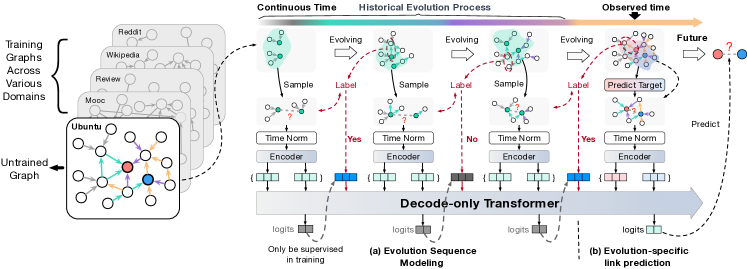
Figure 1: Framework of DyExpert. (a) Models the graph’s evolution process via a sequence of link prediction tasks with ground truths; (b) Evolution-specific link prediction based on both nodes’ representations and the evolution process.

4.1 Overview

This paper centers on the training of a foundation model by multi-domain dynamic graphs that can perform cross-domain link prediction. Intuitively, diverse graphs encompass various physical meanings in cross-domain scenarios, which are harmful for training on numerous graphs and cross-domain generalizing. Hence, we introduce DyExpert, designed for training and inference on diverse datasets. The core idea of DyExpert is straightforward: it conducts link prediction based on the evolving patterns of the corresponding graph. DyExpert trained by conditioned link generation (CLG) that can integrate the modeling of the evolution and link prediction and using caching.

Outline: When conducting a specific link prediction on a given graph, the DyExpert framework unfolds as follows: (1) Depict the graph’s evolution process via a sequence of link prediction tasks with ground-truths; (2) Perform evolution-specific link prediction based on both nodes’ representations and the evolution process. Then in the training stage, we merge (1) and (2) as conditioned link generation for parallel training. And in inference, we adapt caching (1) by QV-caching to accelerate (2).

4.2 Represent Graph Evolution by Sequence

We next show the details of how DyExpert represents the evolution process of a graph by a sequence of link prediction tasks. The evolution of a graph involves an ongoing process of sequential link generation. Naturally, graphs in different domains exhibit distinct generation sequences. Therefore, DyExpert directly models the historic generation sequences of the graphs to learn the evolution pattern.

Consider a dynamic graph $\mathcal{E}_{d}^{t}$ in the domain $d\in\mathcal{D}$ at timestamp $t$. We can sample a series of node pairs from this graph. Formally, the sampled edge pairs are represented as:

$$\tilde{\mathcal{E}}_{d_{K}}^{t_{K}}=\{...(u_{i},v_{i},t_{i},y_{u_{i},v_{i}}^{t_{i}})...(u_{K},v_{K},t_{K},y_{u_{K},v_{K}}^{t_{K}})\}$$ (2)

where $t_{i}<t_{i+1}<t_{K}<t$, $d_{i}=d_{K}=d$, and $y_{u_{i},v_{i}}^{t_{i}}\in\{0,1\}$ denotes whether $u_{i}$ is connected to $v_{i}$ at timestamp $t_{i}$. This sequence of pairs is a subset of the whole link generation process of $\mathcal{E}_{d}^{t}$, which reflects the intrinsic evolution pattern of the graph in domain $d$.

The evolution pattern especially is the correlation between the historical structure of two nodes and their future edge. Therefore, DyExpert uses a graph encoder to obtain the representation of all nodes in $\tilde{\mathcal{E}}_{d_{K}}^{t_{K}}$. Formally, for a pair $(u_{i},v_{i},t_{i},y_{u_{i},v_{i}}^{t_{i}})$, we derive the representations of $u_{i}$ and $v_{i}$ at timestamp $t_{i}$:

$$Z_{u_{i}}^{t_{i}},Z_{v_{i}}^{t_{i}}=\mathbf{GraphEncoder}(\mathcal{G}_{u_{i}}^{t_{i}},\mathcal{G}_{v_{i}}^{t_{i}},\mathcal{T}(t_{*}))$$ (3)

Where $\mathcal{G}_{u_{i}}^{t_{i}}$ is the local sub-graph of $u_{i}$ before $t_{i}$. Since the primary focus of this paper is not on representing the dynamic graph structure, we use $\mathbf{GraphEncoder}(\cdot)$ as a general notation for a dynamic graph representation method. In this paper, we employ DyGFormer (Yu et al., 2023) as the instance of the graph encoder. Then, we can obtain the representation of $\tilde{\mathcal{E}}_{d_{K}}^{t_{K}}$:

$$\mathcal{P}(\tilde{\mathcal{E}}_{d}^{t_{K}})=\{(Z_{u_{0}}^{t_{0}},Z_{v_{0}}^{t_{0}},{y}^{t_{0}}_{u_{0},v_{0}})...(Z_{u_{K}}^{t_{K}},Z_{v_{K}}^{t_{K}},{y}^{t_{K}}_{u_{K},v_{K}})\}$$ (4)

Here, $\mathcal{P}(\tilde{\mathcal{E}}_{d}^{t_{K}})$ is denoted as the evolving sequence in this paper, which contains rich information about $\mathcal{E}_{d}^{t}$. On one hand, the structure distribution of graph of $\mathcal{E}_{d}^{t}$ can be described by $Z_{u_{i}}^{t_{i}}$. On the other hand, the evolving pattern can be reflected by the correlation between node representation and corresponding $y_{u_{*},v_{*}}^{t_{*}}$.

4.3 Link Prediction based on Graph Evolution

Next, DyExpert simultaneously models the gained evolving sequence and the representation of the target node to perform evolution-specific link prediction via transformer.

Let ${u_{K+1},v_{K+1},t_{K+1}}$ denote an edge in domain $d$ to be predicted, where $t_{K+1}>t$. According to our assumption, the predicted $y_{u_{K+1},v_{K+1}}^{t_{K+1}}$ is not only related to the temporal structure of $u_{K+1}$ and $v_{K+1}$ but also to the evolution pattern. To gain a better understanding of the structure of $u_{K+1}$ and $v_{K+1}$, DyExpert employs the same graph encoder $\mathbf{GraphEncoder}(\cdot)$ as in Eq. 2 to model the representation of nodes $u_{K+1}$ and $v_{K+1}$ before timestamp $t_{K}$, denoted as $Z_{u_{K+1}}^{t_{K+1}}$ and $Z_{v_{K+1}}^{t_{K+1}}$. Therefore, $Z_{u_{K+1}}^{t_{K+1}}$ exists in the same representation space as nodes in the sampled evolution pattern, making it easier to model their correlation.

Next, DyExpert integrates the representation of the predicting node pair with the graph evolution pattern represented by $\mathcal{P}(\tilde{\mathcal{E}}_{d}^{t_{K}})$. Given that evolution patterns are described in sequence form, for consistency, the predicting node pair is also treated as a sequence, facilitating their combination through sequence concatenation. Subsequently, DyExpert employs a Transformer to sequentially model them, formalized as:

$$\{...H_{v_{K+1}}\}=\mathbf{Transformer}([\mathcal{P}({\tilde{\mathcal{E}}_{d}^{t_{K}}})||Z_{u_{K+1}}^{t_{K+1}},Z_{v_{K+1}}^{t_{K+1}}])$$ (5)

Note that this is a 12-layer decode-only Transformer (with causality masking), adopted by many foundation models such as GPT-2 (Radford et al., 2019). Its sequential modeling aligns with the graph evolving process as well as our target, namely link prediction based on evolution. Therefore, we use the last hidden state $H_{v_{K+1}}$ to predict the next token, as $H_{v_{K+1}}$ contains all input information and the final prediction result formalized as ${y^{\prime}}_{u_{K+1},v_{K+1}}^{t_{K+1}}=f_{\theta}(H_{v_{K+1}})$, it optimized by cross-entropy with the ground truth, i.e., $\mathbf{CE}({y^{\prime}}_{u_{K+1},v_{K+1}}^{t_{K+1}},{y}_{u_{K+1},v_{K+1}}^{t_{K+1}}))$.

4.4 Training and Inferring

Parallel training by conditioned link generation: Revisiting the representation used to model the evolving $\mathcal{P}(\tilde{\mathcal{E}}_{d}^{t_{K}})$, where each sampled pair is ordered by timestamp, i.e., in $\{...(Z_{u_{i-1}}^{t_{i-1}},Z_{v_{i-1}}^{t_{i-1}},{y}^{t_{i-1}}_{u_{K},v{i-1}}),(Z_{u_{i}}^{t_{i}},Z_{v_{i}}^{t_{i}},{y}^{t_{i}}_{u_{K},v_{i}})...\}$, $t_{i-1}<t_{i}$. Additionally, since $Z_{u_{i}}^{t_{i}}$ and $Z_{v_{i}}^{t_{i}}$ represent the structure before $t_{i}$ if we use $Z_{u_{i}}^{t_{i}}$ and $Z_{v_{i}}^{t_{i}}$ to predict $y_{u_{i},v_{i}}^{t_{i}}$, this process can be treated as a link prediction task based on a shortened evolving pattern. Formally, let $\mathcal{P}(\tilde{\mathcal{E}}_{d}^{t{i-1}})\subset\mathcal{P}(\tilde{\mathcal{E}}_{d}^{t_{K}})$ denote all sampled node pairs before $t_{i}$. This link prediction task can be expressed as:

$$\{...H_{v_{i}}...\}=\mathbf{Transformer}([\mathcal{P}({\mathcal{E}_{d}^{t_{i-1}}})||Z_{u_{i}}^{t_{i}},Z_{v_{i}}^{t_{i}}||...])$$ (6)

Since DyExpert employs a decode-only transformer, the sequence following of $Z_{v_{i}}^{t_{i}}$ does not influence the result of $H_{v_{i}}$. Consequently, based on $H_{v_{i}}$, we can reuse the prediction head to make a link prediction of the following content of $t_{i}$, denoted as ${y^{\prime}}_{u_{i},v_{i}}^{t_{i}}=f_{\theta}(H_{v_{i}})$.

Optimizing ${y^{\prime}}_{u_{i},v_{i}}^{t_{i}}$ offers several advantages. On the one hand, it can enhance the robustness of link prediction with evolving, as it essentially optimizes the predicting results based on evolving sequences of different lengths and combinations. On the other hand, it also can enhance the modeling evolution. Link prediction is modeling the evolution pattern of dynamic graphs. Therefore, the intermediate result of link prediction can reflect the characteristics of evolution patterns. Meanwhile, the modeling of evolution patterns is optimized by successor link prediction which is based on evolution patterns. Therefore, this optimization is typically a multi-task training model for better-comprehending evolution patterns.

Therefore, considering one sample in domain $d$, the loss of DyExpert:

$$\mathcal{L}_{d}(u_{K+1},v_{K+1},t_{K+1})=\sum_{i=1}^{K+1}{\mathbf{CE}({y^{\prime}}_{u_{i},v_{i}}^{t_{i}},{y}_{u_{i},v_{i}}^{t_{i}}))}$$ (7)

Where $d_{i}=d_{K+1}=d$, and $K+1$ is the max evolving sequence number. Since the last predicting pair also have ground truth, so all the pairs essentially generate the next ground-truth current nodes’ representations and previous involution process. Thus, we term the entire process of Eq (7) as conditioned link generation (CLG).

Finally, considering the multi-domain setting, the whole loss of DyExpert is: $\mathcal{L}_{all}=\sum_{d=0}^{\mathcal{D}_{train}}{\mathcal{L}_{d}(*)}$. It is worth noting that different domains would not be cross-sampled. Each computational process of $\mathcal{L}_{d}(*)$ occurred within a single graph in domain $d$. Algorithm 1 in the Appendix shows more details.

Time augmentation: To minimize the disparity in the physical meaning of different graphs, we conduct time normalization for each sub-graph $\mathcal{G}_{u_{i}}^{t_{i}}$ used in Eq (3). In $\mathcal{G}_{u_{i}}^{t_{i}}$, each time $t_{u,*}$ is normalized by $\tilde{t}_{u,*}=\frac{\alpha({t_{i}}-t_{u,*})}{{t_{i}}}$, where the $\alpha$ is super-parameters. Additionally, to enhance the models’ robustness to the temporal aspects and improve their ability to learn from evolving processes in link prediction, we introduce a time shuffle. For all times in one sequence, the normalized time is shuffled using two random seeds, $\hat{t}_{u,*}=\beta(\tilde{t}_{u,*}+\gamma)$. Since the random seeds are consistent for one sequence, DyExpert comprehends the temporal meaning by modeling the context of the sequence.

Efficient inference:

In inference on a downstream graph, the construction of $\tilde{\mathcal{E}}_{d}^{t_{K}}$ in Eq (5) occurs only once. Subsequently, it can be reused for all link predictions. All computation results related to $\tilde{\mathcal{E}}_{d}^{t_{K}}$, including intermediate results in the decode-only transformer, can be cached. Thus, the time complexity during inference is only $O((K+1)C)$ for each prediction, based on caching. Here, $K+1$ represents the sequence length in self-attention and $C$ accounts for all other matrix operations. With the incorporation of engineering optimizations, DyExpert, once trained, can effortlessly conduct efficient inference on very large-scale graphs.

5 Experiment

Table 1: Performance of various methods regarding cross-domain link prediction. We report their Average Precision (average of 3 runs and omit by %) across eight graphs. Methods above the double horizontal lines present adopt cross-domain settings, and “SOTA (End2End)” denotes the best performance of eight baselines in End2End training (See details in Table 9). Bold and underline indicate the best and the second best performance respectively, and ± represents the variance. All subsequent tables utilize the same notations and metrics.

	Enron	UCI	Nearby	Myket	UN Trade	Ubuntu	Mathover.	College
Random	54.85  ±9.26	55.17  ±9.14	52.22  ±9.38	53.06  ±7.05	50.43  ±6.21	53.61  ±5.98	52.47  ±9.92	55.17  ±9.26
TGAT	61.23  ±0.91	82.88  ±0.11	71.50  ±0.36	66.80  ±0.85	51.43  ±1.73	62.51  ±0.24	72.00  ±0.18	82.88  ±0.11
CAWN	81.00  ±1.05	94.16  ±0.01	69.10  ±0.34	71.46  ±0.17	56.20  ±0.58	58.18  ±0.53	68.23  ±0.37	94.16  ±0.01
GraphMixer	55.84  ±2.26	83.66  ±0.04	74.25  ±0.25	59.24  ±2.35	54.69  ±0.03	71.28  ±0.99	79.21  ±0.66	83.66  ±0.04
TCL	75.84  ±0.37	87.08  ±0.28	69.96  ±0.03	67.73  ±0.40	54.26  ±0.27	66.26  ±0.19	74.31  ±0.16	87.08  ±0.28
DyGFormer	90.80  ±0.54	93.86  ±0.19	71.74  ±0.39	71.34  ±0.46	55.17  ±2.37	65.95  ±0.82	75.70  ±0.34	93.86  ±0.19
DyExpert	91.60  ±0.47	96.02  ±0.07	89.61  ±0.92	87.72  ±0.11	60.52  ±0.29	87.44  ±0.76	89.13  ±0.33	96.04  ±0.07
SOTA (End2End)	92.47  ±0.12	95.79  ±0.17	89.32  ±0.05	86.77  ±0.00	66.92  ±0.07	76.91 ±0.12	89.04  ±0.08	94.75  ±0.03

5.1 Experimental Settings

This paper is dedicated to training a foundation model capable of cross-domain link prediction on dynamic graphs without any additional training. To assess the efficacy of DyExpert in this challenging scenario, we conduct an experiment involving 14 datasets and 9 baselines under 2 settings.

Datasets: Referencing prior research and current benchmarks (Yu et al., 2023; Huang et al., 2023), this paper selects 14 unique and distinct graphs. As Table 5 shows, each link prediction task can be associated with a specific real-world application. Six graphs, namely Mooc, Wikipedia (abbreviated as Wiki), LastFM, Review, UN Vote, and Reddit, are randomly chosen for training, collectively comprising eight million dynamic edges. The remaining eight graphs used for training include Enron, UCI, Nearby, Myket, UN Trade, Ubuntu, Mathoverflow (abbreviated as Mathover.), and College. Due to the varying features of nodes across different datasets, we standardize the node and edge features of all data to be 0. Further details can be found in Appendix C.1.

Baselines: We select eight state-of-the-art (SOTA) dynamic graph models as our baselines, including TGAT (Xu et al., 2020), TGN (Rossi et al., 2020), DyRep(Trivedi et al., 2019), Jodie(Kumar et al., 2019), CAWN(Wang et al., 2021b), GraphMixer(Cong et al., 2023), TCL(Wang et al., 2021a), and DyGFormer(Yu et al., 2023). It’s important to note that TGN, DyRep, and Jodie are exclusively utilized under the End2End setting, as their designs are not suitable for cross-domain settings. For additional information, please refer to the Appendix C.2.

Training setting and evaluation metrics: This experiment mainly involves 2 training settings. (1) Cross-domain: all models are trained using the same set of six training graphs and evaluated on the other eight evaluated datasets. (2) End2End: independently train on the train-set and early stopping based on the validation set of 8 evaluated graphs. To enable a comparative analysis of cross-domain link prediction with End2End training, we chronologically split each evaluation dataset into training, validation, and testing sets at a ratio of 70%/15%/15%. Additionally, we employ random negative sampling strategies for evaluation, a common practice in previous research. We report different performances of different models under different settings on the test-set sets. Due to the inclusion of extensive datasets and experiments, all the reported results are the Average Precision (AP) on the test set.

Implementation details:

Our experiment is conducted based on DyGLib (Yu et al., 2023), see Appendix C.2 for more details.

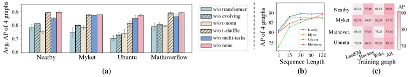
Figure 2: Analysis result of DyExpert regarding multi-domain training. (a) shows the result of ablation studies, where “w/o” removes a certain component of our model. (b) shows the performance of DyExpert adopts different maximum sequence lengths (both training and inference). (c) indicates the performance on evaluated graphs that model solely trained by a specific graph. See more detailed results in Table 10, Table 11, and Table 12, respectively.

5.2 Experiment Result

To assess DyExpert’s effectiveness in cross-domain link prediction, we conduct a comparison with baselines in a cross-domain setting. In this setting, DyExpert and the baselines are trained by six graphs and subsequently evaluated on other eight untrained graphs. We further compare the cross-domain performance with full-supervised baselines (End2End), where baselines are trained by the train-set of each evaluated graph. Importantly, both settings utilized the same test sets. The reported results showcase the best End2End performance across the 8 baselines. Table 1 reveals three key insights from the experiment results:

Insight 1. Link prediction is a generalized task across different domains: (1) Existing baselines naturally demonstrate cross-domain transferability in link prediction. Compared to random prediction, all methods exhibit a 40.33% improvement after training on alternative datasets. Enron, UCI, and College stand out as easily transferable datasets, with the best performance of methods under cross-domain settings on these datasets being only 0.21% lower than the performance of the End2End setting on average. These results suggest that link prediction is a task that can be generalized across diverse domains. (2) However, current methods show instability under cross-domain settings. For example, GraphMixer performs second-best in Nearby and Mathoverflow but struggles in Enron, UCI, and Myket.

Insight 2. DyExpert gains comprehensive improvement on cross-domain link prediction: DyExpert differs from baselines that rely solely on the temporal structure of nodes for predicting links. Instead, DyExpert takes into account both the inherent patterns within predicting graphs and the temporal structure of nodes in link prediction. The experiment results demonstrate that DyExpert achieves significant improvement across various graphs. Compared to the best performance of all baselines under the same training setting, DyExpert showcases a remarkable improvement of over 11.40% (on an average of eight graphs). Particularly on datasets Nearby, Myket, Ubuntu, and Mathoverflow, the average improvement reaches up to 19.66% on average. These results thoroughly illustrate the advancements of DyExpert in cross-domain link prediction.

Insight 3. DyExpert surpasses fully supervised performance on six datasets: Furthermore, we compare DyExpert with the best performance of 8 baselines under End2End (SOTA of End2End). Surprisingly, on these 8 datasets, DyExpert outperforms the SOTA of End2End on 6 datasets, particularly on Ubuntu, with an impressive improvement of nearly 13.69%. For the datasets where DyExpert does not surpass, DyExpert is only 5.25% lower than End2End on average. This exciting result highlights the potential of DyExpert. Furthermore, it validates the feasibility of exploring foundation models for link prediction tasks.

Besides, we also observe the performance of five baselines and DyExpert on the test sets of six training datasets, and it also gains the SOTA performance on them. Besides, we find that training on more datasets indeed leads to poorer performance for some baselines, but DyExpert does not exhibit the same phenomenon. See more details in Table 6.

5.3 Analysis on Multi-domain Training

To delve deeper into why DyExpert performs well, we conduct a comprehensive analysis of its training process. To present the results more clearly, all observations are based on the four most improved datasets, namely Nearby, Myket, Ubuntu, and Mathoverflow. We observe the impact of the model’s different components through ablation studies and then explore the effects of training data and model size.

Insight 4. All components of DyExpert are important: We conducted ablation studies to observe the influence of each component of DyExpert. According to the results shown in Figure 2, we have gathered several observations as follows:

• Modeling evolution drives DyExpert’s performance improvement. When we exclude the evolving pattern (denoted as “w/o evolving”), DyExpert showed an average decrease of 11.11% across four datasets. This outcome suggests that capturing the evolution process is the key to DyExpert’s advancement.

• Multi-task training indeed enhances DyExpert. Multi-task training aids DyExpert in better modeling the evolution sequence. Removing the evolution-based multi-task learning led to an average AP decrease of 2.96% across these four datasets.

• Maximum evolution length can influence model performance: we further explore the impact of the maximum evolution length on the model (i.e., $K+1$ in Eq (5)). As observed, with a rise in the evolution sequence length, the model’s average ranking gradually increases.

• Time normalization is also crucial. Eliminating time normalization (denoted as “w/o t-norm”) results in an average decrease of 13.21% across these datasets. This indicates that although evolution is crucial, it still requires a time normalization that effectively operates on a unified scale. Additionally, appropriately perturbing the normalized time can aid the model in more effective transfer. The removal of random shuffling (“w/o t-shuffle”) also resulted in a decrease of 2.02%.

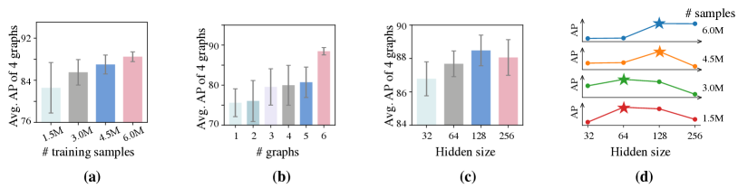
Figure 3: Performance of DyExpert with diverse settings. (a) show the performance of the model improves with more training samples. (b) shows the performance of DyExpert is influenced by the number of training graphs. (c) shows the best-hidden size of the model under 6M training samples. (d) further shows the best-hidden size under different training samples. See more details in Appendix.

Insight 5. Multi-domain training can prompt the model’s generalization: We also compare DyExpert with training on single dataset scenarios. As illustrated in Figure 2 (c), training on single datasets exhibits unstable performance across four datasets. In contrast, training on multi-datasets maintains stability on these four datasets and outperforms the best performance achieved by training on single datasets for each evaluated dataset.

Insight 6. Large-scale and diversity of training datasets and suitable model size also important for DyExpert:

• The model’s performance increases with the expansion of the dataset scale. We train DyExpert under different training sizes (measured by number of edges), which are uniformly sampled from six training datasets. As shown in Figure 3 (a), with the increase in the number of training samples, the model’s performance across four datasets gradually rises. Besides, we also observe changes in the model under different numbers of training datasets. As shown in Figure 3 (b), as the increase of graphs’ number, the model’s performance exhibits overall stable growth.

• The best-hidden size of the model grows with the increase of datasets. We initially show the performance of models with different hidden sizes under 6M training sets. As Figure 3 (c) shows, the best-hidden size of DyExpert is 128. We also examine the best-hidden size under other scales of training sets. As Figure 3 (d) shows as the increase of training datasets, the optimal parameters of the model also decrease from 64 to 128.

• DyExpert exhibits the potential for scale-up. Based on the above results, we observe that under the same parameters, model performance can grow with the scale-up of training data. Besides, as the dataset size increases, the optimal hidden size also gradually rises. This implies that if we continue to increase the scale of training data and incorporate a larger model, we may build a powerful foundation model.

5.4 Analysis on Cross-domain Inferring

We further analyze the properties of DyExpert in cross-domain inference. We first investigate the impact of the sequence length of the evolution sequence in the evaluated graph. Subsequently, we next explore the effects on the model if an inappropriate evolution sequence is employed.

Insight 7. Longer evolving on target dataset can improve the predicting performance: During the inference process, we vary the length of the evolving pattern (denoted as seq-length). As shown in Table 2, the model’s performance steadily increases with the length. This aligns with intuition, as a longer evolution sequence has more information so can better reflect the characteristics of a graph. This result also suggests that DyExpert’s cross-domain link prediction capability is indeed attributed to the modeling of the evolution sequence on the target graph.

Insight 8. We can also use other graphs to activate the model’s performance. We further investigate how the model would behave if link prediction is based on evolving sequences from another graph. As shown in Table 3, the performance varies when models using evolving sequences from some graphs may lead to a decline in the model’s performance on the target dataset, while others do not. On the one hand, this result suggests model indeed models the evolution sequence and makes evolution-specific predictions. On the one hand, it also implies a potential advantage of DyExpert: even when there are not enough edges on the target dataset, we also can use the evolution sequence of graphs similar to the target graph, thereby activating DyExpert’s link prediction capability.

Table 2: Performance of DyExpert with varying evolution sequence lengths. Note that here the model is fixed and only varying lengths of trained models. See more details in Table 7.

Seq length	1	29	59	89	119
Nearby	82.25	85.16	86.69	88.65	89.61
Myket	81.90	87.47	87.50	87.71	87.72
Ubuntu	71.91	79.07	78.79	84.92	87.44
Mathover.	80.42	84.34	84.21	87.31	89.13

Table 3: Performance of DyExpert with evolving patterns from other graphs with 119 sequence length. For comparison, we report the performance under the same domain while the sequence length is only 1. See more details in Table 8.

	# Seq = 1	Evolving pattern of other domain
		Mooc	LastFM	Review	Reddit
Nearby	82.26	80.76	82.00	87.47	84.33
Myket	81.95	79.30	86.23	86.63	87.78
Ubuntu	71.92	75.34	74.96	88.78	79.68
Mathover.	80.43	81.80	81.16	89.10	83.68

6 Conculsion

This paper introduces DyExpert, which explicitly models the evolution process of graphs and conducts evolution-specific link predictions. Extensive experiments are conducted on eight untrained graphs, showcasing the effectiveness of DyExpert in cross-domain link prediction. Detailed analysis results reveal that DyExpert improved by model evolution and exhibits potential. The success of DyExpert demonstrates the feasibility and generalizability of modeling evolution. Besides, DyExpert’s surpassing of fully supervised baselines and the analysis of its scalability both indicate that constructing a foundational model for link prediction tasks is a promising avenue.

Impact Statements

This paper presents work whose goal is to advance the field of Machine Learning. There are many potential societal consequences of our work, none of which we feel must be specifically highlighted here.

Appendix A Dynamic Graph Models

A.1 framework of dynamic graph

Currently, many dynamic graph models based on end2end learning gained advanced performance on link prediction tasks. These methods learn the representation of nodes’ dynamic structure in $\mathcal{E}^{d}_{t}$ and pair-wised predicting future edges. That means their input consists of a node pair with a timestamp $\{u_{i},v_{i},t_{i}\}$, and they output the probability of a link appearing between $u_{i}$ and $v_{i}$ at timestamp $t_{i}$.

More specifically, these works propose various graph encoders to represent the historical temporal structure of nodes. Therefore, when considering a predictive edge pair ${u_{i},v_{i},t_{i}}$, the general framework of a graph encoder is outlined as follows: (1) First, sample local sub-graphs before timestamp $t_{i}$ for these two nodes, denoted as $\mathcal{G}_{u_{i}}^{t_{i}}=\{(e_{u,0},t_{u,0}),(e_{u,1},t_{u,1}),\ldots\}$ and $\mathcal{G}_{v_{i}}^{t_{i}}$. (2) Obtain the initial node/edge features through feature construction and time features using a Time encoder. (3) Feed these features into either a sequence-based neural network or a graph neural network to obtain their respective representations.

For instance, in the sampling strategy of the sub-graph $\mathcal{G}_{u_{i}}^{t_{i}}$, DyGFormer only considers one-hop neighbors (Yu et al., 2023), while CAWN (Wang et al., 2021b) utilizes several sequences based on a time-aware random walk.

A.2 DyGFormer

Here are the details of DyGFormer. DyGFormer only sample nodes 1-hop neighbors. Step 1: Sample 1-hop neighbors of $u$ and $v$:

$\mathcal{N}_{u}^{t}$ = $\{(w_{u,0},t_{u,0}),(w_{u,1},t_{u,1}),...(w_{u,k},t_{u,k})\}$

Step 2: Padding and Time Encoding:

$\mathbf{C}_{\theta}(w_{0})=f_{\theta}(\mathbf{Count}(w_{0},\mathcal{N}_{u}^{t_{i}}))+f_{\theta}(\mathbf{Count}(w_{0},\mathcal{N}_{v}^{t_{i}}))$

$P_{u_{i},k}^{t_{i}}=\mathbf{Concat}(x_{u,k},\mathbf{T}_{\theta}(t_{u,k}),\mathbf{C}_{\theta}({w_{u,k}}))$

$X_{u_{i}}^{t_{i}}=\{P_{u_{i},0}^{t_{i}},P_{u_{i},1}^{t_{i}}...P_{u_{i},K}^{t_{i}}\}$

$\tilde{X}_{u_{i},v_{i}}^{t}=\mathbf{Patch}([X_{u_{i}}^{t_{i}}||X_{v_{i}}^{t_{i}}])$

Step 3: Encoding Transformer:

$Z_{u_{i}}^{t_{i}},Z_{v_{i}}^{t_{i}}=\mathbf{Transformer}(\tilde{X}_{u_{i},v_{i}}^{t})$

Appendix B Algorithm of DyExpert

Here is the details algorithm of DyExpert, note that SortInSeqByTime implies grouping according to SeqNum, sorting only within groups based on time. This randomization and grouping are primarily aimed at ensuring training variability and regularity in negative sample collection, thereby better-maintaining consistency with inference scenarios.

Algorithm 1 Multi-domain training of DyExpert

  Input: $\mathbb{E}=\{\mathcal{E}_{0},...\mathcal{E}_{|\mathcal{D}|}\}$, $m$

  for $epoch$ in Range($maxEpoch$)  do

     $TensorAllData=[]$

     $GroundTruth=[]$

     for $\mathcal{E}_{i}$ in $\mathbb{E}$ do

        $batchSingleData$ = Sample($\mathcal{E}_{i}$)

        for $(u,v,t)$ in $batchSingleData$ do

           $batchSingleData$ = SortByEdgeTime($batchSingleData$)

           $\tilde{v}$ = NegtiveSampe($u,v,\mathcal{E}_{i}$,t)

           $\mathcal{N}_{u},\mathcal{N}_{v},\mathcal{N}_{\tilde{v}}$ = NeighborSample($u,v,\tilde{v},\mathcal{E}_{i}$,t)

           $\mathbf{C}(u,v)$ = CooNeighbor($\mathcal{N}_{u},\mathcal{N}_{v}$)

           $\mathbf{C}(u,\tilde{v})$ = CooNeighbor($\mathcal{N}_{u},\mathcal{N}_{\tilde{v}}$)

           $TensorBatchData$.add([$\mathcal{N}_{u},\mathcal{N}_{v},\mathbf{C}(u,v),PosLabel$])

           $TensorBatchData$.add([$\mathcal{N}_{u},\mathcal{N}_{\tilde{v}},\mathbf{C}(u,\tilde{v}),NegLabel$])

           $BatchGroundTruth$.add(PosLabel)

           $BatchGroundTruth$.add(NegtiveSampe)

        end for

        $randomIndex$ = random()

        $BatchGroundTruth=BatchGroundTruth$[$randomIndex$]

        $TensorBatchData=TensorBatchData$[$randomIndex$]

        $BatchGroundTruth=$ SortInSeqByTime($BatchGroundTruth$,seqNum)

     end for

     $\mathbb{S},\mathbb{R},\mathbb{L}=\mathbf{GraphEncode}(TensorAllData)$

     $evolvingSeq=\mathbf{Concat}$$(\mathbb{S},\mathbb{R},\mathbb{L},dim=1).$reshape(-1,seqNum*3,hiddenSize)

     $hiddenstates=\mathbf{Transformer}(evolvingSeq)$

     $hiddenstates$ = $hiddenstates$.reshape(-1,3,hiddenSize)

     $logitsNextLabel=hiddenstates$[:,1,:]

     $\mathcal{L}=\mathbf{CrossEntropy}$($logitsNextLabel,GroundTruth$)

     $\mathcal{L}$.backward()

  end for

Appendix C Experiment setting

C.1 Datasets

We use $8$ datasets collected by (Poursafaei et al., 2022) in the experiments, which are publicly available in the website:

• Wikipedia can be described as a bipartite interaction graph, which encompasses the modifications made to Wikipedia pages within the span of over a month. In this graph, nodes are utilized to represent both users and pages, while the links between them signify instances of editing actions, accompanied by their respective timestamps. Furthermore, each link is associated with a 172-dimensional Linguistic Inquiry and Word Count (LIWC) feature (Pennebaker et al., 2001). Notably, this dataset also includes dynamic labels that serve to indicate whether users have been subjected to temporary editing bans.

• Reddit is a bipartite network that captures user interactions within subreddits over the course of one month. In this network, users and subreddits serve as nodes, and the links represent timestamped posting requests. Additionally, each link is associated with a 172-dimensional LIWC feature, similar to that of Wikipedia. Furthermore, this dataset incorporates dynamic labels that indicate whether users have been prohibited from posting.

• MOOC refers to a bipartite interaction network within an online educational platform, wherein nodes represent students and course content units. Each link in this network corresponds to a student’s interaction with a specific content unit and includes a 4-dimensional feature to capture relevant information.

• LastFM is a bipartite network that comprises data concerning the songs listened to by users over the course of one month. In this network, users and songs are represented as nodes, and the links between them indicate the listening behaviors of users.

• Enron documents the email communications among employees of the ENRON energy corporation spanning a period of three years.

• UCI represents an online communication network, where nodes correspond to university students, and links represent messages posted by these students.

• UN Trade dataset encompasses the trade of food and agriculture products among 181 nations spanning over a duration of more than 30 years. The weight associated with each link within this dataset quantifies the cumulative value of normalized agriculture imports or exports between two specific countries.

• UN Vote records roll-call votes in the United Nations General Assembly. When two nations both vote ’yes’ on an item, the weight of the link connecting them is incremented by one.

And, we still used other datasets collected from different places:

• Nearby. This dataset contains all public posts and comments, can be downloaded in website

• Ubuntu collected by (Paranjape et al., 2017). A temporal network of interactions on the stack exchange website Ask Ubuntu and every edge represents that user $u$ answered user $v$’s question at time $t$.

• Mathoverflow collected by (Paranjape et al., 2017). A temporal network of interactions on the stack exchange website Mathoverflow and every edge represents that user $u$ answered user $v$’s question at time $t$.

• Review, as described in (Huang et al., 2023), comprises an Amazon product review network spanning the period from 1997 to 2018. In this network, users provide ratings for various electronic products on a scale from one to five. As a result, the network is weighted, with both users and products serving as nodes, and each edge representing a specific review from a user to a product at a specific timestamp. Only users who have submitted a minimum of ten reviews during the mentioned time interval are retained in the network. The primary task associated with this dataset is predicting which product a user will review at a given point in time.

• Myket collected by (Loghmani & Fazli, 2023). This dataset encompasses data regarding user interactions related to application installations within the Myket Android application market.

• College collected by (Panzarasa et al., 2009). This dataset consists of private messages exchanged within an online social network at the University of California, Irvine. An edge denoted as $(u,v,t)$ signifies that user $u$ sent a private message to user $v$ at the timestamp $t$.

Table 4: Statistics of the datasets. Above the dotted line are the six pre-training datasets. #Nodes, #Links, #Src/#Dst, #N&L respectively refer to the number of nodes, the number of links, the ratio of unique source nodes to unique destination nodes within the dataset and the node&link feature dimension(– means not having the feature). Bipartite and Directed indicate whether the graph is a bipartite graph or a directed graph (denoted as 1F5F8 for yes and 2613 for no). / means remaining unknown.

Datasets	Domains	#Nodes	#Links	#Src/#Dst	#N&L Feat	Bipartite	Directed	Duration	Unique Steps	Time Granularity
MOOC	Interaction	7,144	411,749	72.65	– & 4	1F5F8	1F5F8	17 months	345,600	Unix timestamps
LastFM	Interaction	1,980	1,293,103	0.98	– & –	1F5F8	1F5F8	1 month	1,283,614	Unix timestamps
Review	Rating	352,637	4,873,540	1.18	– & –	2613	1F5F8	21 years	6,865	Unix timestamps
UN Vote	Politics	201	1,035,742	1.00	– & 1	2613	1F5F8	72 years	72	years
Wikipedia	Social	9,227	157,474	8.23	– & 172	1F5F8	1F5F8	1 month	152,757	Unix timestamps
Reddit	Social	10,984	672,447	10.16	– & 172	1F5F8	1F5F8	1 month	669,065	Unix timestamps
Enron	Social	184	125,235	0.98	– & –	2613	1F5F8	3 years	22,632	Unix timestamps
UCI	Social	1,899	59,835	0.73	– & –	2613	1F5F8	196 days	58,911	Unix timestamps
Nearby	Social	34,038	120,772	0.80	– & –	2613	1F5F8	21 days	99,224	Unix timestamps
Myket	Action	17,988	694,121	1.25	– & –	1F5F8	1F5F8	/	693,774	/
UN Trade	Economics	255	507,497	1.00	– & 1	2613	1F5F8	32 years	32	years
Ubuntu	Interaction	137,517	280,102	0.75	– & –	2613	1F5F8	2613 days	279,840	days
Mathoverflow	Interaction	21,688	90,489	0.65	– & –	2613	1F5F8	2350 days	107,547	days
College	Social	1,899	59,835	0.73	– & –	2613	1F5F8	193 days	58,911	Unix timestamps

Table 5: The aligned real-world application by each link prediction. Above the dotted line are the six training datasets.

	Type	Real-world Application
MOOC	Course Selecting	Weather a course in a specific content unit selected by a student.
LastFM	Song listened	Weather a particular song was listened to by a user.
Review	Product Reviewed	Weather a product is reviewed in Amazon.
UN Vote	Voting	Weather a nation vote ”yes” on an item in the United Nations General Assembly.
Wikipedia	Entry Editing	Weather a user edited a specific entry in Wikipedia.
Reddit	Social Interaction	Weather user’s interactions within subreddits.
Enron	Email Communication	Weather Two employees in ENRON energy corporation communicate by email.
UCI	Online Communication	Weather messages posted by students in a university.
Nearby	Post Commented	Weather a public post in Nearby is commented.
Myket	App installed	Weather an Android application installations within the Myket Android application market.
UN Trade	International Trade	Weather is a cumulative value of normalized agriculture imports or exports between two specific countries.
Ubuntu	Question Answered	whether a user answered another user’s question in Ask Ubuntu.
Mathoverflow	Question Answered	Weather a user answered another user’s question in Mathoverflow.
College	Online Communication	Weather is a private message sent between students in the University of California, Irvine.

C.2 Implementation details

Our experiment is conducted based on DyGLib (Yu et al., 2023), an open-source toolkit with standard training pipelines including diverse benchmark datasets and thorough baselines.

Due to the varying number of edges in each dataset, we apply duplicate sampling to datasets with fewer edges to ensure consistency in the number of edges for each dataset. Following the setting of (Yu et al., 2023), we employ a 1:1 negative sampling strategy for the edges of each dataset, with three random seeds in both the training and inference phases to ensure that each method is trained or tested with the same negative samples in each randomization.

Our method and baselines utilize the default setup of DyGLib (Yu et al., 2023), with hidden sizes of 128 for time, edge, and node, employing AdamW as the optimizer and linear warm-up. Given the cross-domain scenario and the presence of negative sampling in link prediction, we observed that the validation set of the training data does not necessarily correlate directly with the performance of the evaluated dataset. Considering that real-world scenarios often involve training on the entire dataset and emphasize the robustness of methods, all our models were trained for 50 epochs, and results were reported based on the last epoch. Each model underwent three training iterations with three different random seeds, ensuring consistency in the edges and negative samples seen by all models in each epoch.

For our method, the graph encoder employed DyGFomer with time augmentation. The transformer had 12 layers, 8 attention heads, and a hidden size of 128. All details, including activation functions, layer normalization, and GPT2 decoder, are consistent throughout.

Appendix D Experiment Result

Table 6: Link Prediction AP for training on the single dataset, comparing with training on the all $6$ datasets.

Dataset	Train	TGAT	CAWN	Mixer.	Former.	Ours
Mooc	Single	80.76	83.22	72.09	83.55	83.84
	All	80.67	82.76	67.10	82.99	83.38
	Impv.	-0.11%	-0.56%	-7.44%	-0.67%	-0.55%
Wiki	Single	95.58	99.20	95.99	99.36	99.39
	All	95.21	99.21	91.85	99.31	99.40
	Impv.	-0.39%	-0.06%	-4.51%	-0.05%	+0.01%
LastFM	Single	67.85	86.29	70.74	89.75	91.82
	All	66.22	86.29	58.51	89.73	91.84
	Impv.	-2.46%	+0.00%	-20.90%	-0.02%	+0.02%
Review	Single	72.46	73.26	89.28	85.59	91.54
	All	70.26	77.62	82.90	84.87	91.53
	Impv.	-3.13%	+5.62%	-7.70%	-0.85%	-0.01%
UN Vote	Single	50.59	53.76	50.96	56.71	55.86
	All	50.87	53.98	50.96	56.53	55.63
	Impv.	+0.55%	+0.41%	+0.00%	-0.32%	-0.41%
Reddit	Single	91.33	98.58	91.34	98.98	99.11
	All	91.57	98.49	88.12	98.93	99.11
	Impv.	+0.26%	-0.09%	-3.65%	-0.05%	+0.00%

Table 7: Detailed Link prediction Average Precision (AP) on the unseen datasets across various inference sequence lengths for a model trained by 120 maximum evolving length. ± indicates variance, and the remaining notations in the table are consistent with those in Table 2.

Seq Length	1	29	59	89	119
Nearby	0.8225±0.0065	0.8516±0.0033	0.8669±0.0015	0.8865±0.0133	0.8961±0.0092
Myket	0.8190±0.0139	0.8747±0.0012	0.8750±0.0035	0.8771±0.0023	0.8772±0.0011
Ubuntu	0.7191±0.0009	0.7907±0.0218	0.7879±0.0132	0.8492±0.0174	0.8744±0.0076
Mathoverflow	0.8042±0.0185	0.8434±0.0152	0.8421±0.0046	0.8731±0.0189	0.8913±0.0033

Table 8: Detailed ink prediction Average Precision (AP) on the unseen datasets while using no in-context (# Seq = 1) or using the evolving pattern of other domain with sequence length 120. ±indicates variance, and the remaining notations in the table are consistent with those in Table 3.

	Seq = 1	Using other evolving pattern
		Mooc	LastFM	Review	Reddit
Nearby	0.82255±0.0065	0.80755±0.0106	0.81995±0.0048	0.87465±0.0082	0.84335±0.0072
Myket	0.81950±0.0139	0.79295±0.0093	0.86225±0.0034	0.86625±0.0029	0.87775±0.0008
Ubuntu	0.71915±0.0009	0.75345±0.0109	0.74955±0.0128	0.88775±0.0033	0.79675±0.0110
Mathoverflow	0.80425±0.0185	0.81795±0.0183	0.81155±0.0229	0.89095±0.0053	0.83675±0.0064

Table 9: Link Prediction Average Precision (AP) for End2End training and inferring.

	Enron	UCI	Nearby	Myket	UN Trade	Ubuntu	Mathoverflow	College
TGAT	71.12±0.97	79.63±0.70	83.20 ±0.10	76.32 ±1.03	55.80 ±1.15	76.00 ±0.12	75.18 ±0.03	85.09 ±0.32
TGN	86.53±1.11	92.34±1.04	76.62 ±4.62	85.72 ±0.88	66.84 ±1.13	50.47 ±2.39	62.53 ±1.04	88.37 ±0.27
DyRep	82.38±3.36	65.14±2.30	73.72 ±0.52	86.05 ±0.09	54.61 ±0.48	64.56 ±0.29	73.63 ±0.21	65.72 ±1.87
Jodie	84.77±0.30	89.43±1.09	80.19 ±0.40	86.30 ±0.47	58.11 ±0.61	67.25 ±0.70	77.43 ±0.09	77.08 ±0.48
TCL	79.70±0.71	89.57±1.63	82.13 ±0.43	67.52 ±1.75	54.65 ±0.08	71.93 ±0.86	74.83 ±0.21	87.03 ±0.30
CAWN	89.56±0.09	95.18±0.06	85.01 ±0.16	77.64 ±0.25	61.35 ±0.22	75.05 ±0.40	79.27 ±0.10	94.58 ±0.05
GraphMixer	82.25±0.16	93.25±0.57	89.32 ±0.05	86.77 ±0.00	54.64 ±0.05	84.82 ±0.03	89.04 ±0.08	92.44 ±0.03
DyGFormer	92.47±0.12	95.79±0.17	84.70 ±0.24	85.12 ±0.04	66.92 ±0.07	76.00 ±0.12	80.43 ±0.02	94.75 ±0.03

Table 10: Ablation experiments for DyExpert. Each line indicates the performance for link prediction evaluated by AP when certain aspects of our model’s design are removed.

		Enron	UCI	Nearby	Myket	UN Trade	Ubuntu	Mathoverflow	College
Network Structure	w/o decoder	90.09±0.39	95.89±0.29	78.20±2.19	74.69±3.47	58.43±0.48	70.64±2.12	79.08±2.65	95.89±0.29
	w/o evolving	90.84±0.72	96.08±0.07	81.21±0.14	80.03±0.86	54.72±0.49	72.96±1.88	80.45±1.70	96.09±0.07
Time Processer	w/o t-norm	85.86±0.50	95.47±0.17	75.20±1.11	78.37±1.39	58.68±1.19	74.02±3.03	79.52±0.50	95.47±0.17
	w/o t-shuffle	91.37±0.15	96.25±0.28	89.17±0.27	87.49±0.33	60.35±0.43	81.09 ±2.22	89.07±0.67	95.25±0.28
Training Strategy	w/o multi-datasets	91.08±0.50	95.57±0.08	87.88±0.43	86.70±0.77	57.52±0.88	86.33±0.89	87.01±0.30	95.57±0.08
	w/o multi-tasks	88.20±1.59	95.49±0.13	84.92±0.89	87.23±0.26	57.13±0.26	85.07±2.31	86.16±1.68	95.50±0.13
All Strategy		91.60±0.47	96.02±0.07	89.61±0.92	87.72±0.11	60.52±0.29	87.44±0.76	89.13±0.33	96.04±0.07

Table 11: The performance of link prediction in terms of Average Precision (AP) under various maximum training and inference sequence lengths is presented. The experiments were conducted on the same six datasets with consistent settings throughout. The values in the table represent the mean, and ± indicates the variance.

Maximum of Seq Length	1	15	30	60	120
Enron	90.84±0.72	90.91±0.46	91.56±0.19	91.57±0.50	91.60±0.47
UCI	96.08±0.07	95.82±0.21	95.83±0.20	95.97±0.25	96.02±0.07
Nearby	81.21±0.14	88.12±0.29	89.62±0.29	89.46±0.22	89.61±0.92
Myket	80.03±0.86	87.47±0.20	87.67±0.39	87.45±0.45	87.72±0.11
UNtrade	54.72±0.49	58.35±0.47	58.99±0.86	60.07±0.54	60.52±0.29
Ubuntu	72.96±1.88	82.89±1.83	85.16±2.26	87.44±1.44	87.44±0.76
Mathoverflow	80.45±1.70	84.61±0.36	86.66±2.62	87.07±2.63	89.13±0.33
College	96.09±0.07	95.84±0.21	95.84±0.19	95.78±0.25	96.04±0.07

Table 12: The performance of link prediction, as measured by the Average Precision (AP), was trained on different individual datasets and tested on another dataset. Different rows represent the datasets used for training, while different columns represent the datasets used for testing. The values in the table represent the mean, and ± indicates the variance.

	Mooc	LastFM	Review	UNvote	Wiki	Reddit
enron	82.46±1.91	90.19±1.11	60.14±4.96	71.01±3.76	91.08±0.50	86.58±1.68
UCI	93.02±0.25	95.57±0.08	85.12±2.72	79.56±0.83	95.26±0.16	95.02±0.25
Nearby	76.66±2.02	80.41±0.52	87.88±0.43	55.67±3.13	81.12±0.17	71.97±2.24
Myket	73.60±2.64	86.70±0.77	84.47±0.23	68.14±1.88	86.38±0.24	82.86±2.20
UN Trade	52.09±2.94	57.26±0.40	54.42±4.39	51.65±0.54	57.52±0.88	57.10±0.41
Mathoverflow	80.73±0.80	76.29±3.46	86.33±0.89	61.66±2.63	85.22±0.38	75.58±0.52
Ubuntu	71.46±1.92	68.46±2.59	87.01±0.30	55.63±2.68	78.25±0.44	69.01±0.53
College	93.01±0.25	95.57±0.08	85.12±2.72	79.56±0.83	95.26±0.16	95.03±0.24

Table 13: The Average Precision (AP) of DyExpert trained on a dataset of size 1.5 million for link prediction on an unseen dataset. Bold indicates the best results, underline indicates the second best results, and ± represents the variance.

hidden size	32	64	128	256
Enron	85.29±0.96	86.59±1.98	87.59±0.76	88.41±0.53
UCI	95.86±0.08	95.88±0.30	95.90±0.02	95.81±0.08
Nearby	83.84±0.25	86.21±0.76	85.62±0.51	84.62±1.17
Myket	86.75±0.22	87.51±0.29	87.39±0.45	86.98±0.39
UN Trade	55.21±1.77	55.51±0.48	56.62±0.88	55.97±0.23
Ubuntu	81.10±1.60	82.22±4.38	74.86±1.22	73.69±1.48
Mathoverflow	81.25±0.65	82.58±1.52	82.44±0.84	81.50±1.42
College	95.87±0.08	95.89±0.30	95.90±0.01	95.81±0.09

Table 14: The Average Precision (AP) of DyExpert trained on a dataset of size 3.0 million for link prediction on an unseen dataset. Bold indicates the best results, underline indicates the second best results, and ± represents the variance.

hidden size	32	64	128	256
Enron	90.15±0.25	90.75±0.52	90.67±0.92	90.76±0.61
UCI	96.10±0.18	96.16±0.05	96.16±0.05	95.94±0.15
Nearby	86.81±0.70	87.26±0.33	88.57±1.20	87.20±0.43
Myket	85.04±1.30	87.08±0.79	87.09±0.51	86.77±0.67
UN Trade	58.37±1.22	59.18±1.33	56.39±0.95	58.63±1.03
Ubuntu	83.32±1.50	83.91±0.40	82.55±2.41	79.55±0.73
Mathoverflow	83.58±1.45	84.06±0.29	83.88±0.37	82.95±1.15
College	96.11±0.18	96.17±0.05	95.90±0.01	95.84±0.14

Table 15: The Average Precision (AP) of DyExpert trained on a dataset of size 4.5 million for link prediction on an unseen dataset. Bold indicates the best results, underline indicates the second best results, and ± represents the variance.

hidden size	32	64	128	256
Enron	91.21±0.91	91.84±0.06	91.86±0.24	91.55±0.40
UCI	95.73±0.10	96.15±0.13	95.93±0.05	96.01±0.14
Nearby	87.71±0.13	87.96±0.49	89.49±0.29	88.65±0.47
Myket	86.17±0.43	87.39±0.49	87.52±0.47	86.77±1.33
UN Trade	57.10±2.59	59.48±0.93	58.49±1.54	59.16±0.88
Ubuntu	84.44±1.68	85.81±1.73	84.52±1.52	82.87±1.59
Mathoverflow	84.89±0.63	84.96±1.50	86.46±1.91	84.46±0.64
College	95.75±0.10	96.16±0.13	95.94±0.04	96.01±0.15

Table 16: The Average Precision (AP) of DyExpert trained on a dataset of size 6.0 million for link prediction on an unseen dataset. Bold indicates the best results, underline indicates the second best results, and ± represents the variance.

hidden size	32	64	128	256
Enron	91.76±0.41	91.49±0.38	91.60±0.47	91.47±0.68
UCI	95.69±0.19	95.85±0.22	96.02±0.07	95.60±0.06
Nearby	88.03±0.40	88.90±0.72	89.61±0.92	89.16±0.78
Myket	87.12±0.33	87.68±0.07	87.72±0.11	87.01±0.66
UN Trade	57.33±2.06	59.64±0.65	60.52±0.29	60.58±0.62
Ubuntu	85.20±1.24	87.29±0.73	07.44±0.76	86.97±1.28
Mathoverflow	86.77±1.69	86.83±0.85	89.13±0.33	89.11±0.90
College	95.71±0.19	95.87±0.22	96.04±0.07	95.61±0.07

References

- Anonymous (2024) Anonymous. One for all: Towards training one graph model for all classification tasks. In The Twelfth International Conference on Learning Representations, 2024.
- Bommasani et al. (2021) Bommasani, R., Hudson, D. A., Adeli, E., Altman, R., Arora, S., von Arx, S., Bernstein, M. S., Bohg, J., Bosselut, A., Brunskill, E., et al. On the opportunities and risks of foundation models. arXiv preprint arXiv:2108.07258, 2021.
- Brown et al. (2020) Brown, T., Mann, B., Ryder, N., Subbiah, M., Kaplan, J. D., Dhariwal, P., Neelakantan, A., Shyam, P., Sastry, G., Askell, A., et al. Language models are few-shot learners. Advances in neural information processing systems, 33:1877–1901, 2020.
- Cao et al. (2010) Cao, B., Liu, N. N., and Yang, Q. Transfer learning for collective link prediction in multiple heterogenous domains. In Proceedings of the 27th international conference on machine learning (ICML-10), pp. 159–166. Citeseer, 2010.
- Chakrabarti (2007) Chakrabarti, S. Dynamic personalized pagerank in entity-relation graphs. In Proceedings of the 16th international conference on World Wide Web, pp. 571–580, 2007.
- Cong et al. (2023) Cong, W., Zhang, S., Kang, J., Yuan, B., Wu, H., Zhou, X., Tong, H., and Mahdavi, M. Do we really need complicated model architectures for temporal networks? arXiv preprint arXiv:2302.11636, 2023.
- Devlin et al. (2018) Devlin, J., Chang, M.-W., Lee, K., and Toutanova, K. Bert: Pre-training of deep bidirectional transformers for language understanding. arXiv preprint arXiv:1810.04805, 2018.
- Guo & Chen (2013) Guo, Y. and Chen, X. Cross-domain scientific collaborations prediction using citation. In 2013 IEEE/ACM international conference on advances in social networks analysis and mining (ASONAM 2013), pp. 765–770. IEEE, 2013.
- Hamilton et al. (2017) Hamilton, W., Ying, Z., and Leskovec, J. Inductive representation learning on large graphs. Advances in neural information processing systems, 30, 2017.
- Hoffmann et al. (2022) Hoffmann, J., Borgeaud, S., Mensch, A., Buchatskaya, E., Cai, T., Rutherford, E., Casas, D. d. L., Hendricks, L. A., Welbl, J., Clark, A., et al. Training compute-optimal large language models. arXiv preprint arXiv:2203.15556, 2022.
- Huang et al. (2014) Huang, H., Tang, J., Wu, S., Liu, L., and Fu, X. Mining triadic closure patterns in social networks. In Proceedings of the 23rd international conference on World wide web, pp. 499–504, 2014.
- Huang et al. (2023) Huang, S., Poursafaei, F., Danovitch, J., Fey, M., Hu, W., Rossi, E., Leskovec, J., Bronstein, M., Rabusseau, G., and Rabbany, R. Temporal graph benchmark for machine learning on temporal graphs. arXiv preprint arXiv:2307.01026, 2023.
- Kaplan et al. (2020) Kaplan, J., McCandlish, S., Henighan, T., Brown, T. B., Chess, B., Child, R., Gray, S., Radford, A., Wu, J., and Amodei, D. Scaling laws for neural language models. arXiv preprint arXiv:2001.08361, 2020.
- Kazemi et al. (2020) Kazemi, S. M., Goel, R., Jain, K., Kobyzev, I., Sethi, A., Forsyth, P., and Poupart, P. Representation learning for dynamic graphs: A survey. The Journal of Machine Learning Research, 21(1):2648–2720, 2020.
- Kirillov et al. (2023) Kirillov, A., Mintun, E., Ravi, N., Mao, H., Rolland, C., Gustafson, L., Xiao, T., Whitehead, S., Berg, A. C., Lo, W.-Y., et al. Segment anything. arXiv preprint arXiv:2304.02643, 2023.
- Kossinets & Watts (2006) Kossinets, G. and Watts, D. J. Empirical analysis of an evolving social network. science, 311(5757):88–90, 2006.
- Kumar et al. (2020) Kumar, A., Singh, S. S., Singh, K., and Biswas, B. Link prediction techniques, applications, and performance: A survey. Physica A: Statistical Mechanics and its Applications, 553:124289, 2020.
- Kumar et al. (2019) Kumar, S., Zhang, X., and Leskovec, J. Predicting dynamic embedding trajectory in temporal interaction networks. In Proceedings of the 25th ACM SIGKDD international conference on knowledge discovery & data mining, pp. 1269–1278, 2019.
- Liu et al. (2023a) Liu, J., Yang, C., Lu, Z., Chen, J., Li, Y., Zhang, M., Bai, T., Fang, Y., Sun, L., Yu, P. S., et al. Towards graph foundation models: A survey and beyond. arXiv preprint arXiv:2310.11829, 2023a.
- Liu et al. (2023b) Liu, P., Yuan, W., Fu, J., Jiang, Z., Hayashi, H., and Neubig, G. Pre-train, prompt, and predict: A systematic survey of prompting methods in natural language processing. ACM Computing Surveys, 55(9):1–35, 2023b.
- Loghmani & Fazli (2023) Loghmani, E. and Fazli, M. Effect of choosing loss function when using t-batching for representation learning on dynamic networks, 2023.
- Newman (2001) Newman, M. E. Clustering and preferential attachment in growing networks. Physical review E, 64(2):025102, 2001.
- Panzarasa et al. (2009) Panzarasa, P., Opsahl, T., and Carley, K. M. Patterns and dynamics of users’ behavior and interaction: Network analysis of an online community. Journal of the American Society for Information Science and Technology, 60(5):911–932, 2009.
- Paranjape et al. (2017) Paranjape, A., Benson, A. R., and Leskovec, J. Motifs in temporal networks. In Proceedings of the tenth ACM international conference on web search and data mining, pp. 601–610, 2017.
- Pareja et al. (2020) Pareja, A., Domeniconi, G., Chen, J., Ma, T., Suzumura, T., Kanezashi, H., Kaler, T., Schardl, T., and Leiserson, C. Evolvegcn: Evolving graph convolutional networks for dynamic graphs. In Proceedings of the AAAI conference on artificial intelligence, volume 34, pp. 5363–5370, 2020.
- Pennebaker et al. (2001) Pennebaker, J. W., Francis, M. E., and Booth, R. J. Linguistic inquiry and word count: Liwc 2001. Mahway: Lawrence Erlbaum Associates, 71(2001):2001, 2001.
- Pope et al. (2023) Pope, R., Douglas, S., Chowdhery, A., Devlin, J., Bradbury, J., Heek, J., Xiao, K., Agrawal, S., and Dean, J. Efficiently scaling transformer inference. Proceedings of Machine Learning and Systems, 5, 2023.
- Poursafaei et al. (2022) Poursafaei, F., Huang, S., Pelrine, K., and Rabbany, R. Towards better evaluation for dynamic link prediction. Advances in Neural Information Processing Systems, 35:32928–32941, 2022.
- Radford et al. (2019) Radford, A., Wu, J., Child, R., Luan, D., Amodei, D., Sutskever, I., et al. Language models are unsupervised multitask learners. OpenAI blog, 1(8):9, 2019.
- Radford et al. (2021) Radford, A., Kim, J. W., Hallacy, C., Ramesh, A., Goh, G., Agarwal, S., Sastry, G., Askell, A., Mishkin, P., Clark, J., et al. Learning transferable visual models from natural language supervision. In International conference on machine learning, pp. 8748–8763. PMLR, 2021.
- Rossi et al. (2020) Rossi, E., Chamberlain, B., Frasca, F., Eynard, D., Monti, F., and Bronstein, M. Temporal graph networks for deep learning on dynamic graphs. arXiv preprint arXiv:2006.10637, 2020.
- Snijders (2011) Snijders, T. A. Statistical models for social networks. Annual review of sociology, 37:131–153, 2011.
- Touvron et al. (2023) Touvron, H., Martin, L., Stone, K., Albert, P., Almahairi, A., Babaei, Y., Bashlykov, N., Batra, S., Bhargava, P., Bhosale, S., et al. Llama 2: Open foundation and fine-tuned chat models. arXiv preprint arXiv:2307.09288, 2023.
- Trivedi et al. (2019) Trivedi, R., Farajtabar, M., Biswal, P., and Zha, H. Dyrep: Learning representations over dynamic graphs. In International conference on learning representations, 2019.
- Veličković et al. (2017) Veličković, P., Cucurull, G., Casanova, A., Romero, A., Lio, P., and Bengio, Y. Graph attention networks. arXiv preprint arXiv:1710.10903, 2017.
- Wang et al. (2021a) Wang, L., Chang, X., Li, S., Chu, Y., Li, H., Zhang, W., He, X., Song, L., Zhou, J., and Yang, H. Tcl: Transformer-based dynamic graph modelling via contrastive learning. arXiv preprint arXiv:2105.07944, 2021a.
- Wang et al. (2021b) Wang, Y., Chang, Y.-Y., Liu, Y., Leskovec, J., and Li, P. Inductive representation learning in temporal networks via causal anonymous walks. arXiv preprint arXiv:2101.05974, 2021b.
- Wei et al. (2022) Wei, J., Wang, X., Schuurmans, D., Bosma, M., Xia, F., Chi, E., Le, Q. V., Zhou, D., et al. Chain-of-thought prompting elicits reasoning in large language models. Advances in Neural Information Processing Systems, 35:24824–24837, 2022.
- Xu et al. (2020) Xu, D., Ruan, C., Korpeoglu, E., Kumar, S., and Achan, K. Inductive representation learning on temporal graphs. arXiv preprint arXiv:2002.07962, 2020.
- Ye et al. (2021) Ye, R., Hou, Y., Lei, T., Zhang, Y., Zhang, Q., Guo, J., Wu, H., and Luo, H. Dynamic graph construction for improving diversity of recommendation. In Proceedings of the 15th ACM Conference on Recommender Systems, pp. 651–655, 2021.
- Yu et al. (2023) Yu, L., Sun, L., Du, B., and Lv, W. Towards better dynamic graph learning: New architecture and unified library. arXiv preprint arXiv:2303.13047, 2023.
- Zaki et al. (2016) Zaki, A., Attia, M., Hegazy, D., and Amin, S. Comprehensive survey on dynamic graph models. International Journal of Advanced Computer Science and Applications, 7(2), 2016.
- Zhou et al. (2018) Zhou, L., Yang, Y., Ren, X., Wu, F., and Zhuang, Y. Dynamic network embedding by modeling triadic closure process. In Proceedings of the AAAI conference on artificial intelligence, volume 32, 2018.