$\alpha$-Divergence Loss Function for Neural Density Ratio Estimation

Abstract

Recently, neural networks have produced state-of-the-art results for density-ratio estimation (DRE), a fundamental technique in machine learning. However, existing methods bear optimization issues that arise from the loss functions of DRE: a large sample requirement of Kullback–Leibler (KL)-divergence, vanishing of train loss gradients, and biased gradients of the loss functions. Thus, an $\alpha$-divergence loss function ($\alpha$-Div) that offers concise implementation and stable optimization is proposed in this paper. Furthermore, technical justifications for the proposed loss function are presented. The stability of the proposed loss function is empirically demonstrated and the estimation accuracy of DRE tasks is investigated. Additionally, this study presents a sample requirement for DRE using the proposed loss function in terms of the upper bound of $L_{1}$ error, which connects a curse of dimensionality as a common problem in high-dimensional DRE tasks.

1 Introduction

Density ratio estimation (DRE) is a fundamental technique used in various machine learning (ML) fields. DRE estimates the density ratio $r(\mathbf{x})=q(\mathbf{x})/p(\mathbf{x})$ of two probability densities using two sample sets drawn separately from $p$ and $q$. Several ML methods involve such problems including generative modeling (Goodfellow et al., 2014; Nowozin et al., 2016; Uehara et al., 2016), mutual information estimation and representation learning (Belghazi et al., 2018; Hjelm et al., 2018), energy-based modeling (Gutmann & Hyvärinen, 2010), and covariate shift and domain adaptation (Shimodaira, 2000; Huang et al., 2006). Owing to its potential to leverage various ML methods, the development of an effective DRE method has garnered significant attention.

Recently, neural network methods for DRE have yielded state-of-the-art results. Such methods train neural networks as density ratio functions using loss functions obtained from variational representations of $f$-divergence (Nguyen et al., 2010), which is equivalent to density-ratio matching under Bregman divergence (Sugiyama et al., 2012). The optimal function for a variational representation of $f$-divergence with the Legendre transform corresponds to the density ratio.

However, existing neural network methods offer the following drawbacks. First, Kullback–Leibler (KL)-divergence optimization often fails to train neural networks because optimization requires the sample size to exponentially increase with the true amount of divergence (Poole et al., 2019; Song & Ermon, 2019; McAllester & Stratos, 2020). Second, loss function gradients sometimes vanish when the estimated probability ratios are close to zero or infinity (Arjovsky & Bottou, 2017). Third, for naive loss functions obtained from the variational representation of divergences, gradients over mini-batch samples lead to a biased estimate of the full gradient (Belghazi et al., 2018).

For training neural networks with a large KL-divergence, existing methods address large sample requirements by dividing the KL-divergence estimation into smaller estimations (Rhodes et al., 2020). However, the approach incurs high computational learning and prediction costs. To solve vanishing gradient problems, loss functions with penalties have been proposed (Gulrajani et al., 2017; Roth et al., 2017). Nonetheless, the problems are yet to be solved completely despite extensive efforts. To handle biased loss function gradients, unbiased estimators of the gradients have been proposed (Grover et al., 2019; Yu et al., 2020).

Thus, this study focuses on $\alpha$-divergence, a subgroup of $f$-divergence. $\alpha$-divergence has a sample complexity that is independent of its ground truth value. By selecting $\alpha$ from a particular interval, vanishing gradients of loss functions can be avoided when the optimization of neural network parameters reaches extreme local minima. Additionally, a Gibbs density representation for a variational representation of divergence to obtain unbiased mini-batch gradients is proposed. The proposed loss function is named as $\alpha$-divergence loss function ($\alpha$-Div). Owing to its concise implementation and stability during optimization, $\alpha$-Div offers numerous potential applications.

The proposed approach is empirically justified and the estimation accuracies of DRE tasks are investigated. Furthermore, a sample requirement for DRE using the proposed loss function is presented in terms of the upper bound of $L_{1}$ error. Thereafter, a curse of dimensionality in high-dimensional DRE tasks, which is assumed to be a common problem in DRE, is discussed.

This study is divided into nine parts. First, the background of the study is introduced. Second, notations and problem settings are discussed. Third, a DRE method is described using $f$-divergence variational representations, and its major problems are investigated. Fourth, a novel loss function for DRE is proposed. Fifth, technical justifications for the proposed loss function are presented. Sixth, the stability of the proposed loss function is empirically demonstrated, and the estimation accuracy of DRE tasks is investigated. Seventh, the sample requirement for DRE is discussed using the proposed loss function in terms of the upper bound of $L_{1}$ error. Eighth, related studies are reviewed. Finally, this paper is concluded. All proofs are provided in the appendix.

2 Problem Setup

$P$ and $Q$ are probability distributions on $\Omega\subset\mathbb{R}^{d}$ with unknown probability densities $p$ and $q$, respectively. Assuming $p(\mathbf{x})>0\Leftrightarrow q(\mathbf{x})>0$ at almost everywhere $\mathbf{x}\in\Omega$, the goal of DRE is to accurately estimate $r(\mathbf{x})=q(\mathbf{x})/p(\mathbf{x})$ from given i.i.d. samples $\mathbf{X}_{P}^{(N)}=\{\mathbf{x}_{i}^{p}\}_{i=1}^{N}\sim p$ and $\mathbf{X}_{Q}^{(M)}=\{\mathbf{x}_{i}^{q}\}_{i=1}^{M}\sim q$.

Remark 2.1.

Let $\Omega_{p}$ and $\Omega_{q}$ denote the support of $P$ and $Q$, respectively. Then, $\Omega_{p}=\Omega_{q}$ is assumed in the considered setting, which has an advantage of making clear discussions on vanishing gradient problems. If $\Omega_{q}\subset\Omega_{p}$ is assumed, use only the samples in $\Omega_{q}$ to follow this assumption. Specifically, let $\mathbf{X}_{P\cap Q}^{(N^{\prime})}=\mathbf{X}_{P}^{(N)}\cap\Omega_{q}$. Subsequently, train a neural network model using $\mathbf{X}_{P\cap Q}^{(N^{\prime})}$ and $\mathbf{X}_{Q}^{(M)}$; and then estimate the density ratio $r(\mathbf{x})$ from outputs of the model if $\mathbf{x}\in\Omega_{q}$; otherwise estimate the density ratio such that $r(\mathbf{x})\equiv 0$.

2.1 Additional Notation

$E_{P}[\cdot]$ denotes expectations under the distribution $P$: $E_{P}[f(\mathbf{X})]=\int_{\Omega_{p}}f(\mathbf{x})dP(\mathbf{x})$. $\hat{E}_{P}[\cdot]$ denotes the empirical expectations of $\mathbf{X}_{P}^{(N)}$: $\hat{E}_{P}[f(\mathbf{X})]=\sum_{i=1}^{N}f(\mathbf{x}_{i}^{p})/N$. Similarly, the notation $E_{Q}[\cdot]$ and $\hat{E}_{Q}[\cdot]$ are defined. $E[\cdot]$ is written for $E_{P}[E_{Q}[\cdot]]$.

Table 1: List of loss functions $\mathcal{L}_{f}(\phi_{\theta})$ in Equation (2) of $f$-divergences together with convex functions. A part of the listed divergences and their convex functions is based on Nowozin et al. (2016).

Name	convex function $f$	$\mathcal{L}_{f}(\phi_{\theta})$
Kullback–Leibler (KL)	$u\log u$	$-\hat{E}_{Q}[\log(\phi_{\theta})]+\hat{E}_{P}[\phi_{\theta}]-1$
Reverse KL	$-\log u$	$\hat{E}_{Q}[\phi_{\theta}^{-1}]+\hat{E}_{P}[\log(\phi_{\theta})]-1$
Peason $\chi^{s}$	$(u-1)^{2}$	$-2\hat{E}_{Q}[\phi_{\theta}]+\hat{E}_{P}[\phi_{\theta}^{2}]+1$
Squared Hellinger	$(\sqrt{u}-1)^{2}$	$\hat{E}_{Q}[\phi_{\theta}^{-1/2}]+\hat{E}_{P}[\phi_{\theta}^{1/2}]-2$
GAN	$u\log-(u+1)\log(u+1)$	$\hat{E}_{Q}[\log(1+\phi_{\theta}^{-1})]+\hat{E}_{P}[\log(1+\phi_{\theta})]$

3 DRE via $f$-Divergence Variational Representations and Major Problems

In this section, DRE with $f$-divergence variational representations is introduced. Thereafter, three major problems in existing DRE methods with $f$-divergence variational representations are discussed. First, biased gradient problems of the loss functions are introduced. Second, the sample size requirements for KL-divergence is discussed. Third, vanishing-gradient problems for optimizing divergences are investigated.

Table 2: List of gradient formulas $\nabla_{\theta}\mathcal{L}_{f}(\phi_{\theta})$ of loss functions $\mathcal{L}_{f}(\phi_{\theta})$ given in Table 1 and the destinations of $E[\nabla_{\theta}\mathcal{L}_{f}(\phi_{\theta})]$ as $\phi_{\theta}\rightarrow 0$ or $\phi_{\theta}\rightarrow\infty$ under regular conditions. The symbol “*” denotes undetermined destination as a linear formula of $E_{Q}[\nabla_{\theta}\phi_{\theta}]$ and $E_{P}[\nabla_{\theta}\phi_{\theta}]$.

		$E[\nabla_{\theta}\mathcal{L}_{f}(\phi_{\theta})]\rightarrow\text{?}$
Name	$\nabla_{\theta}\mathcal{L}_{f}(\phi_{\theta})$	$\phi_{\theta}\rightarrow 0$	$\phi_{\theta}\rightarrow\infty$
Kullback–Libler(KL)	$-\hat{E}_{Q}[\nabla_{\theta}\phi_{\theta}/\phi_{\theta}]+\hat{E}_{P}[\nabla_{\theta}\phi_{\theta}]$	*	$E_{Q}[\nabla_{\theta}\phi_{\theta}]$
Reverse KL	$-\hat{E}_{Q}[\nabla_{\theta}\phi_{\theta}/\phi_{\theta}^{2}]+\hat{E}_{P}[\nabla_{\theta}\phi_{\theta}/\phi_{\theta}]$	*	0
Peason $\chi^{s}$	$-2\hat{E}_{Q}[\nabla_{\theta}\phi_{\theta}]+2\hat{E}_{P}[\nabla_{\theta}\phi_{\theta}\cdot\phi_{\theta}]$	$-2E_{Q}[\nabla_{\theta}\phi_{\theta}]$	*
Squared Hellinger	$-\frac{1}{2}\hat{E}_{Q}[\nabla_{\theta}\phi_{\theta}\cdot\phi_{\theta}^{-3/2}]+\frac{1}{2}\hat{E}_{P}[\nabla_{\theta}\phi_{\theta}\cdot\phi_{\theta}^{-1/2}]$	*	0
GAN	$-\hat{E}_{Q}[\nabla_{\theta}\phi_{\theta}/(\phi_{\theta}\cdot(1+\phi_{\theta}))]+\hat{E}_{P}[\nabla_{\theta}\phi_{\theta}/(1+\phi_{\theta})]$	*	0

3.1 DRE with $f$-Divergence Variational Representation

First, the definition of $f$-divergence is reviewed.

Definition 3.1 ($f$-divergence).

The $f$-divergence $D_{f}$ between the two probability measures $P$ and $Q$, induced by a convex function $f$ satisfying $f(1)=0$, is defined as $D_{f}(Q||P)=E_{P}[f(q(\mathbf{x})/p(\mathbf{x}))]$.

Several divergences are specific cases obtained by selecting a suitable generator function $f$. For example, $f(u)=u\log u$ corresponds to KL-divergence.

The variational representations of $f$-divergences are obtained using the Legendre transform of the convex conjugate of a twice differentiable convex function $f$, $f^{*}(\psi)=\sup_{u\in\mathbb{R}}\{\psi\cdot r-f(u)\}$:

$$D_{f}(Q||P)=\sup_{\phi\geq 0}\{E_{Q}[f^{\prime}(\phi)]-E_{P}[f^{*}(f^{\prime}(\phi))]\},$$ (1)

where supremum is considered over all measurable functions $\phi:\Omega\rightarrow\mathbb{R}$ with $E_{Q}[f^{\prime}(\phi)]<\infty$ and $E_{P}[f^{*}(f^{\prime}(\phi))]<\infty$. The maximum value is achieved at $\phi(\mathbf{x})=q(\mathbf{x})/p(\mathbf{x})$.

Then, by replacing $\phi$ in the equation of a neural network model $\phi_{\theta}$, the optimal function for Equation (1) is trained through back-propagation with a loss function, such that

$$\mathcal{L}_{f}(\phi_{\theta})=-\left\{\hat{E}_{Q}[f^{\prime}(\phi_{\theta})]-\hat{E}_{P}[f^{*}(f^{\prime}(\phi_{\theta}))]\right\},$$ (2)

where $\phi_{\theta}$ denotes a real-valued function, such that $\phi_{\theta}(\mathbf{x})\in\mathbb{R}$.

Table 1 lists pairs of convex and loss functions $\mathcal{L}_{f}(\phi_{\theta})$ in Equation (2) for several $f$-divergences.

3.2 Biased Gradient Problem

When a neural network is trained with a loss function $\mathcal{L}_{f}(\phi_{\theta})$ as in Equation (2), its parameters are updated by the addition of a loss function gradient for sub-data obtained from each mini-batch sampling. To obtain unbiased training with the mini-batch samples, the gradients in the mini-batch samples should not have a bias, such that $E[\nabla_{\theta}\mathcal{L}(\theta)_{f}]=\nabla_{\theta}E[\mathcal{L}_{f}(\theta)]$.

However, naive loss functions in Equation (2) often fail to have unbiased gradients. For example, a case of KL-divergence is considered. In the case, $f(u)=u\log u$. Then, $\mathcal{L}_{KL}(\phi_{\theta})\allowbreak=\allowbreak-\hat{E}_{Q}[\log\phi_{\theta}]\allowbreak+\allowbreak\hat{E}_{P}[\phi_{\theta}]-1$ and $\nabla_{\theta}\mathcal{L}_{KL}(\phi_{\theta})\allowbreak=\allowbreak-\hat{E}_{Q}[\nabla_{\theta}(\log\phi_{\theta})]\allowbreak+\allowbreak\hat{E}_{P}[\nabla_{\theta}(\phi_{\theta})]$.

Notably, in the integral over $\Omega$ for $E_{Q}[\cdot]$, $\nabla_{\theta}E_{Q}[\log\phi_{\theta}]=E_{Q}[\nabla_{\theta}(\log\phi_{\theta})]$ does not hold, but it holds for the sample mean $\hat{E}_{Q}$ as observed previously. Subsequently, $\nabla_{\theta}E[\mathcal{L}_{KL}(\phi_{\theta})]\neq E[\nabla_{\theta}\mathcal{L}_{KL}(\phi_{\theta})]$ is observed.

To address such problems, for example, Yu et al. (2020) proposed an unbiased estimator of loss function gradients.

3.3 Sample Size Requirement Problem for KL-Divergence

Training a neural network with a KL-divergence variational representation requires the sample sizes of training data to increase exponentially with the true value of divergence because the sample complexity of KL-divergence is $O(e^{KL(Q||P)})$ (Poole et al., 2019; Song & Ermon, 2019; McAllester & Stratos, 2020):

$$\lim_{N\rightarrow\infty}N\cdot\mathrm{Var}\Big{[}\widehat{KL^{N}}(Q||P)\Big{]}\geq e^{KL(Q||P)}-1,$$ (3)

where $\widehat{KL^{N}}(Q||P)$ is the KL-divergence estimator for sample size $N$ that uses a variational representation of divergence, and $KL(Q||P)$ is the ground truth value of divergence.

Owing to such high sample complexity, training a neural network with KL-divergence loss function tends to fail particularly in cases of high-dimensional data.

Thus, existing methods divide a high divergence estimation into small divergence estimations (Rhodes et al., 2020). However, the approach incurs high computational cost.

3.4 Vanishing Gradient Problem

Vanishing gradient problems for optimizing divergence are known in generative adversarial networks (GANs) (Goodfellow et al., 2014; Arjovsky & Bottou, 2017). A part of the problems is believed to occur when the following two conditions are satisfied: ($\rm{i}$) The loss function slightly updates the model parameters. ($\rm{ii}$) Updating the model parameters causes little change in the model outputs. Thus, the problem can be assumed to occur when the following relations hold:

$$\underbrace{E[\nabla_{\theta}\mathcal{L}_{f}(\phi_{\theta})]=\vec{0}}_{\text{(}\rm{i}\text{)}}\ \ \text{\&}\ \ \underbrace{E_{Q}[\nabla_{\theta}\phi_{\theta}]=\vec{0}\ \ \text{\&}\ \ E_{P}[\nabla_{\theta}\phi_{\theta}]=\vec{0}}_{\text{(}\rm{ii}\text{)}},$$ (4)

where $\vec{0}$ denotes a vector of zeros of the same size as the model parameters.

Further, a case where the estimated density ratio is either very small or large is considered, allowing the relations in Equation (4) to arise. Table 2 lists the gradient formulas of the divergence loss functions presented in Table 1 and the asymptotic values of the loss gradients as $\phi_{\theta}\rightarrow 0$ or $\phi_{\theta}\rightarrow\infty$. With constants $c_{1}$ and $c_{2}$ in Table 2, cases where $E[\nabla_{\theta}\mathcal{L}_{f}(\phi_{\theta})]=c_{1}\cdot E_{Q}[\nabla_{\theta}\phi_{\theta}]+c_{2}\cdot E_{P}[\nabla_{\theta}\phi_{\theta}]$ as $\phi_{\theta}\rightarrow 0$ or $\phi_{\theta}\rightarrow\infty$ are found, such that the relations in Equation (4) can hold.

In summary, all divergence loss functions presented in Tables 1 and 2 can fall into their vanishing gradients when the estimated density ratio approaches extreme local minima. Notably, the discussed case includes a case of overfitting pointed out by Kato & Teshima (2021), in which train losses of a neural network become extremely small.

To prevent vanishing gradients of train losses, loss functions with penalties have been proposed (Gulrajani et al., 2017; Roth et al., 2017).

4 DRE using a Neural Network with an $\alpha$-Divergence Loss

In this section, the proposed loss function is derived from a variational representation of $\alpha$-divergences. Then, training and prediction methods using the loss function are presented. The exact claims and proofs for all theorems in this section are provided under B.3 in the appendix.

4.1 Derivation of the Proposed Loss Function for DRE

The definition of $\alpha$-divergence, a subgroup of $f$-divergences, is expressed as

$$D_{\alpha}(Q||P)=E_{P}\left[\frac{1}{\alpha(\alpha-1)}\left\{\left(\frac{q(\mathbf{x})}{p(\mathbf{x})}\right)^{1-\alpha}-1\right\}\right],$$ (5)

where $\alpha\in\mathbb{R}\setminus\{0,1\}$. From Equation (5), Hellinger divergence is obtained as $\alpha=1/2$, while $\chi^{2}$ divergence is given by $\alpha=-1$.

Then, the variational representation of $\alpha$-divergence is given by the following.

Theorem 4.1.

A variational representation of $\alpha$-divergence is given as

$$D_{\alpha}(Q||P)\!\!\!\! = \!\!\!\!\sup_{\phi\geq 0}\left\{\frac{1}{\alpha(1-\alpha)}-\frac{1}{\alpha}E_{Q}\left[\phi^{\alpha}\right]\qquad\qquad\right.$$ (6)

$$\left.\quad\qquad-\quad\frac{1}{1-\alpha}E_{P}\left[\phi^{\alpha-1}\right]\right\},$$

where supremum is considered over all measurable functions with $E_{P}[\phi^{1-\alpha}]<\infty$ and $E_{Q}[\phi^{-\alpha}]<\infty$. The maximum value is achieved at $\phi(\mathbf{x})=q(\mathbf{x})/p(\mathbf{x})$.

Generally, as $\nabla_{\theta}E_{Q}[\phi_{\theta}^{\alpha}]\allowbreak\neq\allowbreak E_{Q}[\nabla_{\theta}(\phi_{\theta}^{\alpha})]$ and $\nabla_{\theta}E_{P}[\phi_{\theta}^{\alpha-1}]\allowbreak\neq\allowbreak E_{P}[\nabla_{\theta}(\phi_{\theta}^{\alpha-1})]$, the naive loss function obtained from the right-hand side of Equation (6) has biased gradients. By rewriting the terms $\phi_{\theta}^{\alpha}$ and $\phi_{\theta}^{\alpha-1}$ in the Gibbs density expression, unbiased gradients of the proposed loss function can be obtained. Subsequently, another variational representation of $\alpha$-divergence is as follows.

Theorem 4.2.

A variational representation of $\alpha$-divergence is given as

$$D_{\alpha}(Q||P)\!\!\!\! = \!\!\!\!\sup_{T:\Omega\rightarrow\mathbb{R}}\left\{\frac{1}{\alpha(1-\alpha)}-\frac{1}{\alpha}E_{Q}\left[e^{\alpha\cdot T}\right]\right.$$ (7)

$$\left.\quad\qquad-\quad\frac{1}{1-\alpha}E_{P}\left[e^{(\alpha-1)\cdot T}\right]\right\},$$

where supremum is considered over all measurable functions $T:\Omega\rightarrow\mathbb{R}$ with $E_{P}[e^{(\alpha-1)\cdot T}]<\infty$ and $E_{Q}[e^{\alpha\cdot T}]<\infty$. Equality holds for $T^{*}$, thereby satisfying $e^{-T^{*}(\mathbf{x})}=q(\mathbf{x})/p(\mathbf{x})$.

Therefore, from the aforementioned representations, the proposed loss function for DRE is obtained, which is named as $\alpha$-divergence loss function ($\alpha$-Div).

Definition 4.3 ($\alpha$-Div).

$\alpha$-Divergence loss is defined as follows:

$$\mathcal{L}_{\alpha}^{(N,M)}(T_{\theta})\!\!\!\! = \!\!\!\!\frac{1}{\alpha}\hat{E}_{Q}\left[e^{\alpha\cdot T_{\theta}}\right]+\frac{1}{1-\alpha}\hat{E}_{P}\left[e^{(\alpha-1)\cdot T_{\theta}}\right]$$ (8)

$$= \!\!\!\!\frac{1}{\alpha}\cdot\frac{1}{M}\cdot\Sigma_{i=1}^{M}e^{\alpha\cdot T_{\theta}(\mathbf{x}_{i}^{q})}$$

$$+\ \ \frac{1}{1-\alpha}\cdot\frac{1}{N}\cdot\Sigma_{i=1}^{N}e^{(\alpha-1)\cdot T_{\theta}(\mathbf{x}_{i}^{p})}.$$

The superscript variable “$(N,M)$” is dropped when unnecessary in the context and represented as $\mathcal{L}_{\alpha}(T_{\theta})$.

Theorem 4.2 can be rewritten for $\alpha$-Div as follows.

Theorem 4.4.

Let $T^{*}$ be the optimal function for the following infimum

$$T^{*}\!\!\!\! = \!\!\!\!\arg\inf_{T:\Omega\rightarrow\mathbb{R}}E[\mathcal{L}_{\alpha}(T)]$$ (9)

$$= \!\!\!\!\arg\inf_{T:\Omega\rightarrow\mathbb{R}}\left\{\frac{1}{\alpha}E_{Q}\left[e^{\alpha\cdot T}\right]\right.$$

$$\left.\quad\qquad+\quad\frac{1}{1-\alpha}E_{P}\left[e^{(\alpha-1)\cdot T}\right]\right\},$$

where infimum is considered over all measurable functions $T:\Omega\rightarrow\mathbb{R}$ with $E_{P}[e^{(\alpha-1)\cdot T}]<\infty$ and $E_{Q}[e^{\alpha\cdot T}]<\infty$. Then, $T^{*}$ represents the energy function of the density ratio $q(\mathbf{x})/p(\mathbf{x})$, such that $T^{*}(\mathbf{x})=-\log(q(\mathbf{x})/p(\mathbf{x}))$.

4.2 Training and Predicting with $\alpha$-Div

Algorithm 1 Training for DRE with $\alpha$-Div

  Input: Data from a denominator distribution $\{\mathbf{x}_{i}^{p}\}_{i=1}^{N}$, and from a numerator distribution $\{\mathbf{x}_{i}^{q}\}_{i=1}^{M}$.

  Output: A neural network model $T_{\theta_{K}}$.

  for $t=1$ to $t_{\max}$ do

     $\hat{E}_{P}\leftarrow\frac{1}{N}\Sigma_{i=1}^{N}e^{(\alpha-1)\cdot T_{\theta_{t}}(\mathbf{x}_{i}^{p})}$

     $\hat{E}_{Q}\leftarrow\frac{1}{M}\Sigma_{i=1}^{M}e^{\alpha\cdot T_{\theta_{t}}(\mathbf{x}_{i}^{q})}$

     $\mathcal{L}_{\alpha}({\theta_{t}})\leftarrow\hat{E}_{Q}/\alpha+\hat{E}_{P}/(1-\alpha)$

     $\theta_{t+1}\leftarrow\theta_{t}-\nabla_{\theta_{t}}\mathcal{L}_{\alpha}({\theta_{t}})$

  end for

Training a neural network with $\alpha$-Div is shown in Algorithm 1. Practically, neural networks rarely achieve infimum as in Equation (9). Therefore, normalizing the naive estimated values of neural networks is efficient in achieving better optimization. The following theorem justifies the normalization of the estimated values.

Theorem 4.5.

For a fixed function $T:\Omega\rightarrow\mathbb{R}$, let $c_{*}$ be the optimal scaler value for the follwoing infimum

$$c_{*}\!\!\!\! = \!\!\!\!\arg\inf_{c\in\mathbb{R}}E[\mathcal{L}_{\alpha}(T+c)]$$ (10)

$$= \!\!\!\!\arg\inf_{c\in\mathbb{R}}\left\{\frac{1}{\alpha}E_{Q}\left[e^{\alpha\cdot(T+c)}\right]\right.$$

$$\left.\quad\qquad+\quad\frac{1}{1-\alpha}E_{P}\left[e^{(\alpha-1)\cdot(T+c)}\right]\right\}.$$

Then, $c_{*}$ satisfies $e^{c_{*}}=E_{P}\left[e^{-T}\right]$, or equivalently, $e^{-(T+c_{*})}=e^{-T}/E_{P}\left[e^{-T}\right]$.

Consequently, the target density ratio can be estimated as follows.

Estimated density ratio using outputs of $T_{\theta}(\mathbf{x})$ in Algorithm 1:

$$\widehat{\frac{q(\mathbf{x})}{p(\mathbf{x})}}=\frac{e^{-T_{\theta}(\mathbf{x})}}{\hat{E}_{P}\left[e^{-T_{\theta}}\right]}$$ (11)

5 Theoretical Justifications of $\alpha$-Div

In this section, theoretical results that justify the proposed approach with $\alpha$-Div, which can solve all problems mentioned in Section 3, are discussed. The exact claims and proofs for all theorems in this section are provided under Section B.4 in the appendix.

5.1 Unbiasedness of Gradients

Theorem 5.1 guarantees unbiased gradients of $\alpha$-Div.

Theorem 5.1 (brief and informal).

Let $T_{\theta}(\mathbf{x}):\Omega\rightarrow\mathbb{R}$ be a function such that the map $\theta=(\theta_{1},\theta_{2},\ldots,\theta_{p})\in\Theta\mapsto T_{\theta}(\mathbf{x})$ is differentiable for all $\theta$ and $\mu$ at almost every $\mathbf{x}\in\Omega$. Then, under some regular conditions for $T_{\theta}$, Equation (12) holds such that

$$E\left[\nabla_{\theta}\mathcal{L}_{\alpha}(\theta)|_{\theta=\bar{\theta}}\right]=\nabla_{\theta}E\left[\mathcal{L}_{\alpha}(\theta)\right]|_{\theta=\bar{\theta}}.$$ (12)

5.2 Sample Size Requirements

The sample requirement of $\alpha$-Div does not exceed a specific value that depends on $\alpha$. Intuitively, such a property of $\alpha$-Div comes from the boundedness of $\alpha$-divergences, such that $0\leq D_{\alpha}\leq 1/(\alpha\cdot(1-\alpha))$. Theorem 5.2 provides the exact upper bond of the $\alpha$-Div sample requirement, which corresponds to Equation (3) for KL-divergence.

Theorem 5.2.

Let $T^{*}=-\log(q(\mathbf{x})/p(\mathbf{x}))$. Subsequently, let

$$\hat{D}_{\alpha}^{(N)}(Q||P)=\frac{1}{\alpha(1-\alpha)}-\mathcal{L}^{(N,N)}_{\alpha}(T^{*}).$$ (13)

Then,

$$\sqrt{N}\left\{\hat{D}_{\alpha}^{(N)}(Q||P)-D_{\alpha}(Q||P)\right\}\xrightarrow{\ \ d\ \ }\mathcal{N}(0,\sigma_{\alpha})$$ (14)

holds, where

$$\sigma_{\alpha}^{2}\!\!\!\! = \!\!\!\!C^{1}_{\alpha}\cdot D_{2\alpha}(Q||P)+C^{2}_{2\alpha}\cdot D_{1-2\alpha}(Q||P)$$

$$\ +C^{3}_{\alpha}\cdot D_{\alpha}(Q||P)^{2}+C^{4}_{\alpha}\cdot D_{\alpha}(Q||P)+C^{5}_{\alpha},$$

and $C^{1}_{\alpha}=2\alpha\cdot(1-2\alpha)/\alpha^{2}$, $C^{2}_{\alpha}=2\alpha\cdot(1-2\alpha)/(1-\alpha)^{2}$, $C^{3}_{\alpha}=-1/\alpha^{2}-1/(1-\alpha)^{2}$, $C^{4}_{\alpha}=2/\alpha^{2}+2/(1-\alpha)^{2}$, and $C^{5}_{\alpha}=(1/\alpha^{2}+1/(1-\alpha)^{2})\cdot(2-2\alpha\cdot(1-\alpha))$.

5.3 Addressing Gradient Vanishing Problem

$\alpha$-Div can avoid vanishing gradients of its train losses by setting $\alpha$ within $(0,1)$.

First, the gradients of $\alpha$-Div are obtained.

$$\nabla_{\theta}\mathcal{L}_{\alpha}(\theta)=\hat{E}_{Q}\Big{[}\nabla_{\theta}T_{\theta}\cdot e^{\alpha\cdot T_{\theta}}\Big{]}-\hat{E}_{P}\Big{[}\nabla_{\theta}T_{\theta}\cdot e^{(\alpha-1)\cdot T_{\theta}}\Big{]}.$$ (16)

Then, the case where the probability ratio $e^{T_{\theta}(\mathbf{x})}$ in Equation (16) is nearly zero or large for any point $\mathbf{x}\in\Omega$ is considered. Notably, under the assumption that $p(\mathbf{x})>0\Leftrightarrow q(\mathbf{x})>0$ for $\forall\mathbf{x}\in\Omega$, $E_{Q}[e^{T_{\theta}}]\rightarrow 0\Leftrightarrow E_{P}[e^{T_{\theta}}]\rightarrow 0$ and $E_{Q}[e^{T_{\theta}}]\rightarrow\infty\Leftrightarrow E_{P}[e^{T_{\theta}}]\rightarrow\infty$ are observed. Then, the behavior of $E[\nabla_{\theta}\mathcal{L}_{\alpha}(\theta)]$ when $E_{P}[e^{T_{\theta}}]\rightarrow 0$ or $E_{P}[e^{T_{\theta}}]\allowbreak\rightarrow\allowbreak\infty$, under some regular conditions for $T_{\theta}$, can be summarized as

$\alpha>1$:

$$E[\nabla_{\theta}\mathcal{L}_{\alpha}(\theta)]\!\!\!\! \rightarrow \!\!\!\!\vec{0}\quad\text{as}\ \ E_{P}[e^{T_{\theta}}]\rightarrow 0,\ \ \ \text{and}$$ (17)

$$E[\nabla_{\theta}\mathcal{L}_{\alpha}(\theta)]\!\!\!\! \rightarrow \!\!\!\!\vec{\infty}-\vec{\infty}\ \ \text{as}\ \ E_{P}[e^{T_{\theta}}]\rightarrow\infty.$$ (18)

$\alpha<0$:

$$E[\nabla_{\theta}\mathcal{L}_{\alpha}(\theta)]\!\!\!\! \rightarrow \!\!\!\!\vec{0}\quad\text{as}\ \ E_{P}[e^{T_{\theta}}]\rightarrow\infty,\ \ \ \text{and}$$ (19)

$$E[\nabla_{\theta}\mathcal{L}_{\alpha}(\theta)]\!\!\!\! \rightarrow \!\!\!\!\vec{\infty}-\vec{\infty}\ \ \text{as}\ \ E_{P}[e^{T_{\theta}}]\rightarrow 0.$$ (20)

$0<\alpha<1$:

$$E[\nabla_{\theta}\mathcal{L}_{\alpha}(\theta)]\!\!\!\! \rightarrow \!\!\!\!-\vec{\infty}\ \ \text{as}\ \ E_{P}[e^{T_{\theta}}]\rightarrow 0,\ \ \ \text{and}$$ (21)

$$E[\nabla_{\theta}\mathcal{L}_{\alpha}(\theta)]\!\!\!\! \rightarrow \!\!\!\!\vec{\infty}\ \quad\text{as}\ \ E_{P}[e^{T_{\theta}}]\rightarrow\infty.$$ (22)

For $\alpha>1$ and $\alpha<0$, cases where $E[\nabla_{\theta}\mathcal{L}_{\alpha}(\theta)]\allowbreak\rightarrow\vec{0}$ as found in Equations (17) and (19) exist. Thus, the possibility that the neural networks reach extreme local minima such that their estimations for density ratios are $0$ or $\infty$ arises. However, the problem can be avoided by selecting $\alpha$ from the interval $(0,1)$. Moreover, the selection of $\alpha$ does not cause instability in numerical calculations for cases where $E[\nabla_{\theta}\mathcal{L}_{\alpha}(\theta)]\rightarrow\vec{\infty}-\vec{\infty}$, as in Equations (18) and (20).

6 Experiments

In this section, the stability of $\alpha$-Div over optimization for diverse values of $\alpha$, as discussed in Section 3.4, is empirically demonstrated. Next, the $L^{2}$ error of $\alpha$-Div in DRE tasks is investigated using synthetic datasets.

6.1 Experiments on Stability during Optimization for Different Values of $\alpha$

First, the stability of $\alpha$-Div over optimization for diverse values of $\alpha$ was demonstrated. For $\alpha=-3,\allowbreak-2,\allowbreak-1,\allowbreak 0.2,\allowbreak 0.5,\allowbreak 0.8,\allowbreak 2.0,\allowbreak 3.0$, and $4.0$, neural network models with synthetic datasets over 100 trials were trained while measuring the training loss of $\alpha$-Div for each learning step. Then, the median, the range of the 45th–55th, and the 5th–95th quartiles of the training loss were reported at each learning step.

Experimental Setup.

Synthetic data of size 5000 were generated from 5-dimensional normal distribution $\{X_{1},X_{2},\ldots,X_{5}\}$ with $E[X_{i}]=0$, $\mathrm{Var}[X_{i}]=1$, and $E[X_{i}\cdot X_{j}]=0.8$ ($i\neq j$). A 100×4 perceptron with ReLU activation was used. The Adam algorithm in PyTorch was employed. The learning rate of the hyperparameters in the training was 0.001, BathSize was 2500, and the number of epochs was 250. The other hyperparameter settings in the training of the neural networks are presented in Section C in the appendix.

Results.

The training loss results of $\alpha$-Div for each learning step during optimization are shown in Figure 1. The $y$-axis of each graph represents the training loss of $\alpha$-Div, whereas the $x$-axis represents the learning step. The solid blue line indicates the median of the training losses. The dark blue area shows the training loss ranges between the 45th and 55th quartiles, while the light blue area shows that between the 5th and 95th quartiles.

As shown in the top and center figures of Figure 1, the training losses of $\alpha$-Div diverged to large negative values for $\alpha=-3,-2,-1,2.0,3.0$, and $4.0$. However, as shown in the bottom figures of Figure 1, optimizations with $\alpha$-Div were stable, such that its training losses converged for $\alpha=0.2,0.5$, and $0.8$.

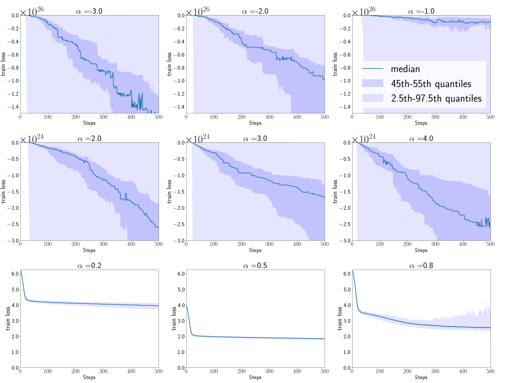
Figure 1: Results of Section 6.1 for $\alpha=-3,-2,-1,0.2,0.5,0.8,2.0,3.0$, and $4.0$. The $y$-axis of each graph represents training losses of $\alpha$-Div, while the $x$-axis of each graph represents the learning step. The solid blue line indicates the median of the training losses of $\alpha$-Div. The dark blue area shows the ranges of the training losses between the 45th and 55th quartiles, while the light blue area shows that between the 5th and 95th quartiles.

6.2 Experiments on $L^{2}$ Error in DRE using Synthetic Datasets

The $L^{2}$ error in DRE tasks was investigated using $\alpha$-Div. The experimental setup provided by Kato & Teshima (2021) was followed. The mean squared errors (MSEs) of DRE tasks were measured for synthetic datasets using state-of-the-art DRE methods and $\alpha$-Div over 100 trials. The average mean and standard deviation of all results were reported.

Experimental Setup.

The proposed method was compared with Kullback-Leibler importance estimation procedure (KLIEP) (Sugiyama et al., 2007), unconstrained least-Squares importance fitting (uLSIF) (Kanamori et al., 2009), and deep direct DRE (D3RE) (Kato & Teshima, 2021). The densratio library in R was used for KLIEP and uLSIF. For D3RE, nnBD-LSIF and a 100×3 perceptron with ReLU activation, which was used in experiments by Kato & Teshima (2021), were used. The hyperparameter $C$ of D3RE was set at 2.0. For $\alpha$-Div, the same neural network structure as for D3RE was used. For both D3RE and $\alpha$-Div, the neural networks were trained with a common learning rate of SGD, but with different epoch sizes tuned with small parts of the datasets. The other hyperparameter settings for each method are presented in Section C in the appendix.

Let the dimensions of the synthetic dataset be $d$, where $d=10,20,30,50$ and $100$. First, 100 datasets of training and test data were generated, each of which comprised 1000 samples of $d$-dimensional data from $P=\mathcal{N}(\mu_{p},I_{d})$ and $q=\mathcal{N}(\mu_{q},I_{d})$. Herein, $I_{d}$ denotes a $d$-dimensional identity matrix, and $\mu_{p}$ and $\mu_{q}$ represent $d$-dimensional vectors with $\mu_{p}=(0,0,\ldots,0)$ and $\mu_{q}=(1,0,\ldots,0)$, respectively. For each dataset, the model parameters were optimized using the training data, and then the density ratios for the test data were estimated. The MSEs of the estimated density ratios and the true density ratios of the test data were measured. Furthermore, the average mean and standard deviation of all results for the aforementioned methods were reported.

Table 3: Results of Section 6.2. The average mean and standard deviation of MSEs in the DRE tasks obtained using the synthetic datasets. The results from 100 simulations are in the form of “mean (std. err.)”. The lowest MSEs are highlighted in bold.

MODEL	Dim=10	Dim=20	Dim=30	Dim=50	Dim=100
KLIEP	2.141(0.392)	2.072(0.660)	2.005(0.569)	1.887(0.450)	1.797(0.419)
uLSIF	1.482(0.381)	1.590(0.562)	1.655(0.578)	1.715(0.446)	1.668(0.420)
D3RE	1.111(0.314)	1.127(0.413)	1.219(0.458)	1.222(0.305)	1.369(0.355)
$\alpha$-Div	1.036(0.236)	1.032(0.266)	1.117(0.325)	1.191(0.265)	1.343(0.308)

Results.

The obtained results are presented in Table 3. From the results of KLIEP, six cases where the MSE was greater than 1000 were excluded.

For all data dimensions, $\alpha$-Div estimated more accurately than the other methods with a lower MSE. However, when the data dimensions were 50 and 100, the results of $\alpha$-Div were close to those of D3RE. The DRE results for the high-dimensional datasets suggested an extremely important phenomenon for DRE tasks: a curse of dimensionality in $L_{1}$ error of DRE. This phenomenon is further investigated, as discussed in the next section.

7 Limitations: A Curse of Dimensionality in $L_{1}$ error of DRE

In this section, a sample requirement of $\alpha$-Div in terms of the upper bound of $L_{1}$ error is presented. Then, a curse of dimensionality in high-dimensional DRE tasks, which is a common problem in DRE, is discussed.

Unfortunately, the following upper bound of $L_{1}$ error in estimation is obtained for $\alpha$-Div.

Theorem 7.1 (brief and informal).

Assuming $\Omega$, the support of $p$ and $q$, to be a compact set in $\mathbb{R}^{d}$ with $d\geq 2$. Let $\mathcal{T}_{\text{Lip}}$ be the set of all locally Lipschitz continuous functions that minimize $\mathcal{L}_{\alpha}^{(N,M)}$ for validation data. Additionally, for $T\in\mathcal{T}_{\text{Lip}}$, let $\widehat{\frac{q(\mathbf{x})}{p(\mathbf{x})}}^{T}$ denote the estimated density ratio with $T$ obtained from Equation (11), and let $K=\min\{N,M\}$.

Then, ($\mathrm{i}$) if $r(\mathbf{x})=p(\mathbf{x})/q(\mathbf{x})$ is Lipschitz continuous on $\Omega$, Equation (23) holds for any $T\in\mathcal{T}_{\text{Lip}}$ such that

$$E_{P}\left|\widehat{\frac{q(\mathbf{x})}{p(\mathbf{x})}}^{T}-\ \frac{q(\mathbf{x})}{p(\mathbf{x})}\right|\leq O\left(\left(\frac{1}{K}\right)^{\frac{1}{d}}\right).$$ (23)

In addition, ($\mathrm{ii}$) if $r(\mathbf{x})=p(\mathbf{x})/q(\mathbf{x})$ is bi-Lipschitz continuous on $\Omega$, then there exists $T_{0}\in\mathcal{T}_{\text{Lip}}$ such that

$$E_{P}\left|\widehat{\frac{q(\mathbf{x})}{p(\mathbf{x})}}^{T_{0}}-\ \frac{q(\mathbf{x})}{p(\mathbf{x})}\right|=O\left(\left(\frac{1}{K}\right)^{\frac{1}{d}}\right).$$ (24)

Notably, when $\Omega$ is a compact set, $q(\mathbf{x})/p(\mathbf{x})$ is bounded and has a positive minimum value on $\Omega$ in the considered setting. According to Theorem 7.1, when $p$ and $q$ are positive over $\Omega$, a sample size of $O\left(\left(\frac{1}{\varepsilon}\right)^{d}\right)$ is required to guarantee $\left|\widehat{\frac{q(\mathbf{x})}{p(\mathbf{x})}}-\frac{q(\mathbf{x})}{p(\mathbf{x})}\right|<\varepsilon$ on average.

From a technical perspective, such a sample requirement for the upper bound in $L_{1}$ estimation error would hold for other divergence loss functions $\mathcal{L}_{f}$ because Theorem 7.1 is mainly derived from the consistency of the estimation with $\mathcal{L}_{\alpha}$ (Theorem B.12 in the appendix) and the convergence rate of the expected value of the distance between two neighboring samples (Lemma B.13 in the appendix). Additionally, the sample requirement is considered natural with the following interpretation: to obtain an accurate DRE in a multi-dimensional space, a sample size of data sufficient to fill the space is required. Further research should be performed to address this problem.

8 Related Work

First, studies on DRE using variational representations of $f$-divergences are reviewed. DRE tasks have gained significant attention in various ML fields. For this work, studies on ($\rm{i}$) direct density ratio estimation, ($\rm{ii}$) GANs, and ($\mathrm{iii}$) energy-based models (EBM) are focused. For DRE using variational representations of $f$-divergences, Nguyen et al. (2010) proposed DRE and divergence estimation using variational representations of $f$-divergences. Sugiyama et al. (2012) proposed density-ratio matching under Bregman divergence. As Sugiyama et al. (2012) mentioned, DRE using variational representations of $f$-divergences and density-ratio matching under the Bregman divergence are equivalent. In recent studies, Kato & Teshima (2021) proposed a correction method for Bregman divergence loss functions to prevent the loss functions from overfitting. For GANs, $f$-divergences are used as discriminators (Nowozin et al., 2016). Uehara et al. (2016) highlighted the relations between discriminators of GANs and DRE. For EBMs, this study is included in EBMs (LeCun et al., 2006). We refer readers to Song & Kingma (2021) for a detailed description of the existing methods for training EBMs. Yu et al. (2020), for example, proposed a training method for EBMs using variational representations of $f$-divergences.

Next, studies of the problems in Section 3 are reviewed. Biased gradient problems have been extensively studied in the context of Variational inference (VI) (Kingma & Welling, 2013). Hernandez-Lobato et al. (2016) reduced a baias of gradients of an $\alpha$-divergence loss function. Geffner & Domke (2020) proposed a method for correcting a baias of gradients of an $\alpha$-divergence loss function, which also provided a detailed review of its problem. For DRE using KL-divergence, Rhodes et al. (2020) and Choi et al. (2022) proposed methods to address the sample requirement of large KL-divergences. The vanishing gradient problem of train losses has been studied primarily in the context of optimizing GANs (Gulrajani et al., 2017; Roth et al., 2017).

In addition to the aforementioned studies, researchers have attempted to improve divergences (Birrell et al., 2022).

9 Conclusion

A novel loss function for DRE $\alpha$-Div that provides concise implementation and stable optimization was proposed in this paper. Technical justifications for the proposed loss function were discussed. In the experiments of this study, the effectiveness of the proposed loss function was empirically demonstrated and the estimation accuracy of DRE tasks was investigated. Finally, the sample size requirements for DRE in terms of the upper bound of $L_{1}$ error was confirmed, and then the curse of dimensionality that occurs as a common problem in high-dimensional DRE tasks was discussed. Although the curse of dimensionality remains in the proposed approach, we believe that this study provides a basic method for DRE.

Impact of This Study

This paper presents work whose goal is to advance the field of Machine Learning. There are many potential societal consequences of our work, none which we feel must be specifically highlighted here.

Appendix A Organization of the supplementary

The organization of this supplementary document is as follows: In Section B, we present proofs of the theorems and propositions referenced in this study; In Section C, the details of the experimental settings of Section 6 are provided; In addition to this material, the code used in the numerical experiments is also submitted as supplementary material.

Appendix B Proofs

In this Section, we provide the theorems and proofs referred to in this study. First, we provide notations and Terminologies usded in proofs in the appendix. Next, we present the definition of the $\alpha$-Divergence loss in the manner of probability theory. Then, we provide the theorems and proofs refered to in each section.

B.1 Notations and Terminologies in Appendix

In this section, we provide the notations and terminologies used in proofs in the appendix. Additionally, we summarize all notations used in the appendix in Table 4.

Capital, small and bold letters.

Random variables are denoted by capital letters; for example, $A$. Small letters are used for the values of random variables of the corresponding capital letters; $a$ is the value of the random variable $A$. Bold letters $\mathbf{A}$ or $\mathbf{a}$ represent a set of variables or random variable values. For example, the domain of the variable $A$ is denoted by $\mathcal{X}_{A}$, and $\mathcal{X}_{A_{1}}\times\cdots\times\mathcal{X}_{A_{n}}$ is denoted by $\mathcal{X}_{\mathbf{A}}$ for $\mathbf{A}=A_{1}\times\cdots\times A_{n}$.

Notations and terminologies for the measure theory.

$\Omega$ denotes a subset in $\mathbb{R}^{d}$. $P$ and $Q$ are used as the probability measures on $(\Omega,\mathscr{F})$, where $\mathscr{F}$ denotes the $\sigma$-algebra on $\Omega$. subsets of $\mathbb{R}^{d}$. $P$ is called absolute continuous with respect to $Q$, $P(A)=0$ whenever $Q(A)=0$ for any $A\in\mathscr{F}$, which is represented as $P\ll Q$. $\frac{dP}{dQ}$ denotes the Radon–Nikodým derivative of $P$ with respect to $Q$ for $P$ and $Q$ with $P\ll Q$. In this study, we refer to density ratios as the Radon–Nikodým derivatives. $\mu$ denotes a probability measure on $\Omega$ with $P\ll\mu$ and $Q\ll\mu$. One example of $\mu$ is $(P+Q)/2$.

Table 4: Notations and definitions used in the proofs

Notations	Definitions, Meanings
(Capital,	Random variables are denoted by capital letters; for example, $A$. Small letters are used for the
small and	values of random variables of the corresponding capital letters; $a$ is the value of the random
bold letters)	variable $A$. Bold letters $\mathbf{A}$ or $\mathbf{a}$ represent a set of variables or random variable values.
$\Omega$	A subset in $\mathbb{R}^{d}$: $\Omega\subset\mathbb{R}^{d}$.
$\|\cdot\|$	The euclidean norm.
$O(a_{n})$	The boundedness with rate $a_{n}$: $f(a_{n})=O(a_{n})$ $\Leftrightarrow$ $\lim_{n\rightarrow\infty}|f(a_{n})/a_{n}|\leq C$ with some $C>0$.
$O_{p}(a_{n})$	The stochastic boundedness with rate $a_{n}$ in $\mu$: $\mathbf{X}=O_{p}(a_{n})\Leftrightarrow$ $\forall$ $\varepsilon>0$, $\exists\delta>0$ s.t. $\mu(|\mathbf{X}|>\delta)<\varepsilon$.
$P\ll Q$	$P$ is absolutely continuous with respect to $Q$.
$P$, $Q$	A pair of probability measures with $P\ll Q$ and $Q\ll P$.
$\mu$	A probability measure with $P\ll\mu$ and $Q\ll\mu$.
$\frac{dP}{dQ}$	The Radon–Nikodým derivative of $P$ with respect to $Q$.
$\mathbf{X}_{P}^{(N)}$	$N$ i.i.d. random variables obtained from $P$, which correspond to $N$ samples drawn from $P$:
	$\mathbf{X}_{P}^{(N)}=\{\mathbf{X}^{1}_{\sim P},\mathbf{X}^{2}_{\sim P},\ldots,\mathbf{X}^{N}_{\sim P}\}$, $\mathbf{X}^{i}_{\sim P}\overset{\mathrm{iid}}{\sim}P$.
$\mathbf{X}_{Q}^{(M)}$	$M$ i.i.d. random variables obtained from $Q$, which correspond to $M$ samples drawn from $Q$:
	$\mathbf{X}_{Q}^{(M)}=\{\mathbf{X}^{1}_{\sim Q},\mathbf{X}^{2}_{\sim Q},\ldots,\mathbf{X}^{M}_{\sim Q}\}$, $\mathbf{X}^{i}_{\sim Q}\overset{\mathrm{iid}}{\sim}Q$.
$K$	$K=\min\{N,M\}$.
$\mathcal{L}_{\alpha}^{(N,M)}(T)$	$\alpha$-Divergence loss function. See Definition B.1 in Section B.2.
$\widetilde{l}_{\alpha}\left(\mathbf{x},\mathbf{y};T\right)$	$\widetilde{l}_{\alpha}\left(\mathbf{x},\mathbf{y};T\right)=\frac{1}{\alpha}e^{\alpha\cdot T(\mathbf{x})}\cdot\frac{dQ}{d\mu}(\mathbf{x})+\frac{1}{1-\alpha}e^{(\alpha-1)\cdot T(\mathbf{y})}\cdot\frac{dP}{d\mu}(\mathbf{x})$. See Lemma B.4 in Section B.4.
$\mathbf{X}^{(K)}$	$K$ i.i.d. random variables from $\mu$: $\mathbf{X}^{(K)}=\{\mathbf{X}^{1},\mathbf{X}^{2},\ldots,\mathbf{X}^{K}\}$, $\mathbf{X}^{i}\overset{\mathrm{iid}}{\sim}\mu$.
$\mathbf{X}_{(1)}(\mathbf{x})$	The nearest neighbor variable of $\mathbf{x}$ in $\mathbf{X}^{(K)}$. Specifically, let $\mathbf{X}_{(1)}(\mathbf{x})$ be $\mathbf{X}_{i}$ in $\mathbf{X}^{(K)}$ such that
	$\|\mathbf{X}_{i}-\mathbf{x}\|<\|\mathbf{X}_{j}-\mathbf{x}\|$ ($\forall j<i$) and $\|\mathbf{X}_{i}-\mathbf{x}\|\leq\|\mathbf{X}_{j}-\mathbf{x}\|$ ($\forall j>i$).
$V_{i}$	A nearest neighborhood of $\mathbf{X}_{i}$: $V_{i}=\{\mathbf{y}\in\Omega\ |\ \|\mathbf{X}_{i}-\mathbf{y}\|=\|\mathbf{X}_{(1)}(\mathbf{y})-\mathbf{y}\|\}$.
$\widetilde{\mathcal{L}}_{\alpha}^{(K)}(T)$	$\mu$-approximation of $\alpha$-Divergence loss function $\mathcal{L}_{\alpha}^{(N,M)}(T)$. See Definition B.10 in Section B.5.
$B(\mathbf{a},r)$	The Euclidean ball in $\mathbb{R}^{d}$ with radius $r$: $B(\mathbf{a},r)=\{\mathbf{x}\in\mathbb{R}^{d}|\ \|\mathbf{x}-\mathbf{a}\|<r\}$.
$\bar{B}_{\mathbf{x}}$	A neighborhood of $\mathbf{x}$ within a radius of $\|\mathbf{X}_{(1)}(\mathbf{x})-\mathbf{x}\|$: $\bar{B}_{\mathbf{x}}=\{\mathbf{y}\in\Omega\ |\ \|\mathbf{y}-\mathbf{x}\|\leq\|\mathbf{X}_{(1)}(\mathbf{x})-\mathbf{x}\|\}$.
$\mathrm{diag}(\mathcal{B})$	The diameter of $\mathcal{B}$: $\mathrm{diag}(\mathcal{B})=\inf_{r\in\mathbb{R}}\{\mathcal{B}\subseteq B(\mathbf{a},r)\ |\ \exists\mathbf{a}\in\mathcal{B}\ \}$.

B.2 Definition of $\alpha$-Div

Definition B.1 ($\alpha$-Divergence loss).

Let $\mathbf{X}_{P}^{(N)}=\{\mathbf{X}^{1}_{\sim P},\mathbf{X}^{2}_{\sim P},\ldots,\mathbf{X}^{N}_{\sim P}\}$, $\mathbf{X}^{i}_{\sim P}\overset{\mathrm{iid}}{\sim}P$ denote $N$ i.i.d. random variables from $P$, and let $\mathbf{X}_{Q}^{(M)}=\{\mathbf{X}^{1}_{\sim Q},\mathbf{X}^{2}_{\sim Q},\ldots,\mathbf{X}^{M}_{\sim Q}\}$, $\mathbf{X}^{i}_{\sim Q}\overset{\mathrm{iid}}{\sim}Q$ denote $M$ i.i.d. random variables from $Q$. Then, $\alpha$-Divergence loss $\mathcal{L}_{\alpha}^{(N,M)}$ is defined as follows:

$$\mathcal{L}_{\alpha}^{(N,M)}(T)=\frac{1}{\alpha}\cdot\frac{1}{M}\cdot\Sigma_{i=1}^{M}e^{\alpha\cdot T(\mathbf{X}^{i}_{\sim Q})}+\frac{1}{1-\alpha}\cdot\frac{1}{N}\cdot\Sigma_{i=1}^{N}e^{(\alpha-1)\cdot T(\mathbf{X}^{i}_{\sim P})}.$$ (25)

B.3 Proofs for Section 4

In this Section, we provide the theorems and proofs referred to in Section 4.

Theorem B.2.

A variational representation of $\alpha$-divergence is given as

$$D_{\alpha}(Q||P) = \sup_{\phi\geq 0}\left\{\frac{1}{\alpha(1-\alpha)}-\frac{1}{\alpha}E_{Q}\left[\phi^{-\alpha}\right]-\frac{1}{1-\alpha}E_{P}\left[\phi^{1-\alpha}\right]\right\},$$ (26)

where supremum is considered over all measurable functions with $E_{P}[\phi^{1-\alpha}]<\infty$ and $E_{Q}[\phi^{-\alpha}]<\infty$. The maximum value is achieved at $\phi=dQ/dP$.

proof of Theorem B.2.

Let $f_{\alpha}(t)=\{t^{1-\alpha}-(1-\alpha)\cdot t-\alpha\}/\{\alpha(\alpha-1)\}$ for $\alpha\neq 0,1$, then

$$E_{P}\left[f_{\alpha}\left(\frac{dQ}{dP}\right)\right] = E_{P}\left[\frac{1}{\alpha(\alpha-1)}\left(\frac{dQ}{dP}\right)^{1-\alpha}+\frac{1}{\alpha}\left(\frac{dQ}{dP}\right)+\frac{1}{1-\alpha}\right]$$ (27)

$$= \frac{1}{\alpha(\alpha-1)}E_{P}\left[\left(\frac{dQ}{dP}\right)^{1-\alpha}\right]+\frac{1}{\alpha}+\frac{1}{1-\alpha}$$

$$= D_{\alpha}(Q||P).$$

Note that, the Legendre transform for $g_{\alpha}(x)=\mathbf{x}^{1-\alpha}/(1-\alpha)$ is obatined as

$$g_{\alpha}^{*}(x)=\frac{\alpha}{\alpha-1}x^{1-\frac{1}{\alpha}}.$$ (28)

In addition, note that, for the Legendre transforms of any fuction $h(x)$, it hold that

$$\{C\cdot h(x)\}^{*}=C\cdot h^{*}\left(\frac{x}{C}\right)\quad\text{and}\quad\{h(x)+C\cdot t+D\}^{*}=h^{*}(x-C)-D.$$ (29)

Here, $A^{*}$ denotes the the Legendre transform of $A$.

From (28) and (29), we have

$$f_{\alpha}^{*}(t) = \left\{\frac{1}{(-\alpha)}g_{\alpha}(t)+\frac{1}{\alpha}t+\frac{1}{1-\alpha}\right\}^{*}$$ (30)

$$= \frac{1}{(-\alpha)}g_{\alpha}^{*}\left(-\alpha\cdot\left\{t-\frac{1}{\alpha}\right\}\right)-\frac{1}{1-\alpha}$$

$$= -\frac{1}{\alpha}g_{\alpha}^{*}\left(1-\alpha t\right)+\frac{1}{\alpha-1}$$

$$= -\frac{1}{\alpha}\left\{\frac{\alpha}{\alpha-1}\left(1-\alpha t\right)^{1-\frac{1}{\alpha}}\right\}+\frac{1}{\alpha-1}$$

$$= \frac{1}{1-\alpha}\left(1-\alpha t\right)^{1-\frac{1}{\alpha}}+\frac{1}{\alpha-1}.$$

By differentiating $f_{\alpha}(t)$, we obtain

$$f_{\alpha}^{\prime}(t)=-\frac{1}{\alpha}t^{-\alpha}+\frac{1}{\alpha}.$$ (31)

Thus, we have

$$E_{Q}\left[f_{\alpha}^{\prime}(\phi)\right]=E_{Q}\left[-\frac{1}{\alpha}\phi^{-\alpha}+\frac{1}{\alpha}\right].$$ (32)

From (30) and (31), we obtain

$$E_{P}\left[f_{\alpha}^{*}(f_{\alpha}^{\prime}(\phi))\right] = E_{P}\left[\frac{1}{1-\alpha}\left\{1-\alpha\cdot\left(-\frac{1}{\alpha}\phi^{-\alpha}+\frac{1}{\alpha}\right)\right\}^{1-\frac{1}{\alpha}}+\frac{1}{\alpha-1}\right]$$ (33)

$$= E_{P}\left[\frac{1}{1-\alpha}\phi^{1-\alpha}+\frac{1}{\alpha-1}\right].$$

In additionm, from (32) and (33), we see for both $E_{P}[\phi^{1-\alpha}]<\infty$ and $E_{Q}[\phi^{-\alpha}]<\infty$ to hold is equivalent for both $E_{P}\left[f_{\alpha}^{*}(f_{\alpha}^{\prime}(\phi))\right]<\infty$ and $E_{Q}\left[f_{\alpha}^{\prime}(\phi)\right]<\infty$ to hold.

Finally, substituting (32) and (33) for (1), we have

$$D_{\alpha}(Q||P) = \sup_{\phi\geq 0}\{E_{Q}[f_{\alpha}^{\prime}(\phi)]-E_{P}[f_{\alpha}^{*}(f_{\alpha}^{\prime}(\phi))]\}$$

$$= \sup_{\phi\geq 0}\left\{E_{Q}\left[-\frac{1}{\alpha}\phi^{-\alpha}+\frac{1}{\alpha}\right]-E_{P}\left[\frac{1}{1-\alpha}\phi^{1-\alpha}+\frac{1}{\alpha-1}\right]\right\}$$

$$= \sup_{\phi\geq 0}\left\{\frac{1}{\alpha(1-\alpha)}-\frac{1}{\alpha}E_{Q}\left[\phi^{-\alpha}\right]-\frac{1}{1-\alpha}E_{P}\left[\phi^{1-\alpha}\right]\right\}.$$

Thus, the proof is complete. ∎

Theorem B.3 (Theorem 4.2 in Section 4 is restated).

$\alpha$-divergence can be written as follows:

$$D_{\alpha}(Q||P)=\sup_{T:\Omega\rightarrow\mathbb{R}}\left\{\frac{1}{\alpha(1-\alpha)}-\frac{1}{\alpha}E_{Q}\left[e^{\alpha\cdot T}\right]-\frac{1}{1-\alpha}E_{P}\left[e^{(\alpha-1)\cdot T}\right]\right\},$$ (34)

where supremum is considered over all measurable functions $T:\Omega\rightarrow\mathbb{R}$ with $E_{P}[e^{(\alpha-1)\cdot T}]<\infty$ and $E_{Q}[e^{\alpha\cdot T}]<\infty$. The equality holds for $T^{*}$ satisfying

$$\frac{dQ}{dP}=e^{-T^{*}}.$$ (35)

proof of Theorem 4.2.

Substituting $e^{-T}$ for $\phi$ in (26), we have

$$D_{\alpha}(Q||P) = \sup_{\phi\geq 0}\left\{\frac{1}{\alpha(1-\alpha)}-\frac{1}{\alpha}E_{Q}\left[\phi^{-\alpha}\right]-\frac{1}{1-\alpha}E_{P}\left[\phi^{1-\alpha}\right]\right\}$$ (36)

$$= \sup_{T:\Omega\rightarrow\mathbb{R}}\left\{\frac{1}{\alpha(1-\alpha)}-\frac{1}{\alpha}E_{Q}\left[\left\{e^{-T}\right\}^{-\alpha}\right]-\frac{1}{1-\alpha}E_{P}\left[\left\{e^{-T}\right\}^{1-\alpha}\right]\right\}$$

$$= \sup_{T:\Omega\rightarrow\mathbb{R}}\left\{\frac{1}{\alpha(1-\alpha)}-\frac{1}{\alpha}E_{Q}\left[e^{\alpha\cdot T}\right]-\frac{1}{1-\alpha}E_{P}\left[e^{(\alpha-1)\cdot T}\right]\right\}.$$

Finally, from Lemma B.2, the equality for (36) holds if and only if

$$\frac{dQ}{dP}=e^{-T^{*}}.$$ (37)

Thus, the proof is complete. ∎

Lemma B.4.

For a measurable functions $T:\Omega\rightarrow\mathbb{R}$ with $E_{P}[e^{(\alpha-1)\cdot T}]<\infty$ and $E_{Q}[e^{\alpha\cdot T}]<\infty$, let

$$\widetilde{l}_{\alpha}\left(T(\mathbf{x})\right) = \frac{1}{\alpha}e^{\alpha\cdot T(\mathbf{x})}\frac{dQ}{d\mu}(\mathbf{x})+\frac{1}{1-\alpha}e^{(\alpha-1)\cdot T(\mathbf{x})}\frac{dp}{d\mu}(\mathbf{x}).$$ (38)

Then the optimal function $T^{*}$ for $\inf_{T:\Omega\rightarrow\mathbb{R}}\widetilde{l}_{\alpha}\left(T\right)$ is obtained as $T^{*}=-\log dQ/dP$, $\mu$-almost everywhere.

proof of Lemma B.4.

First, note that it follows from Jensen’s inequality that

$$\log(p\cdot X+q\cdot Y)\geq p\cdot\log(X)+q\cdot\log(Y),$$ (39)

for $X,Y>0$ and $p,q>0$ with $p+q=1$, and the equality holds when $X=Y$.

From this equation, by letting $X=e^{\alpha\cdot T(\mathbf{x})}\cdot\frac{dQ}{d\mu}(\mathbf{x})$, $Y=e^{(\alpha-1)\cdot T(\mathbf{x})}\cdot\frac{dP}{d\mu}(\mathbf{x})$, $p=1-\alpha$ and $q=\alpha$, we observe that

$$\log(p\cdot X+q\cdot Y)=\log\left(\frac{1}{\alpha\cdot(1-\alpha)}\cdot\widetilde{l}_{\alpha}(T)\right),$$

and $\log\left(\frac{1}{\alpha\cdot(1-\alpha)}\cdot\widetilde{l}_{\alpha}(T)\right)$ is minimized when $e^{\alpha\cdot T(\mathbf{x})}\cdot\frac{dQ}{d\mu}(\mathbf{x})=e^{(\alpha-1)\cdot T(\mathbf{x})}\cdot\frac{dP}{d\mu}(\mathbf{x})$, $\mu$-almost everywhere.

Then, we see that $\inf_{T:\Omega\rightarrow\mathbb{R}}\widetilde{l}_{\alpha}(T)$ is achieved at $e^{-T^{*}(\mathbf{x})}=\frac{dQ}{dP}(\mathbf{x})$, $\mu$-almost everywhere. Hence, we have $T^{*}(\mathbf{x})=-\log dQ/dP(\mathbf{x})$, $\mu$-almost everywhere.

∎

Lemma B.5.

For a measurable functions $T:\Omega\rightarrow\mathbb{R}$ with $E_{P}[e^{(\alpha-1)\cdot T}]<\infty$ and $E_{Q}[e^{\alpha\cdot T}]<\infty$, let

$$L_{\alpha}(T) = E_{\mu}\left[\widetilde{l}_{\alpha}\left(T(\mathbf{x})\right)\right]$$ (40)

$$= \frac{1}{\alpha}\cdot E_{Q}\left[e^{\alpha\cdot T(\mathbf{X})}\right]+\frac{1}{1-\alpha}\cdot E_{P}\left[e^{(\alpha-1)\cdot T(\mathbf{X})}\right],$$ (41)

and let

$$\widetilde{l}_{\alpha}^{*} = \inf_{T:\Omega\rightarrow\mathbb{R}}\widetilde{l}_{\alpha}(T),$$ (42)

$$L_{\alpha}^{*} = \inf_{T:\Omega\rightarrow\mathbb{R}}L_{\alpha}(T),$$ (43)

where the infimums of (42)-(43) are considered over all measurable functions with $T:\Omega\rightarrow\mathbb{R}$ with $E_{P}[e^{(\alpha-1)\cdot T}]<\infty$ and $E_{Q}[e^{\alpha\cdot T}]<\infty$.

Then, it holds that

$$E_{\mu}\left[\widetilde{l}_{\alpha}(T)\right]=L_{\alpha}(T),$$ (44)

$$E_{\mu}\left[\widetilde{l}_{\alpha}^{*}\right]=L_{\alpha}^{*}.$$ (45)

Additionally, the equalities in (42) and (43) hold for $T^{*}=-\log dQ/dP$.

proof of Lemma B.5.

We first show the last equality in (45) holds. Now, we consider the following integral:

$$E\left[\frac{1}{\alpha(1-\alpha)}-\widetilde{l}_{\alpha}^{*}\right] = \int\left\{\frac{1}{\alpha(1-\alpha)}-\widetilde{l}_{\alpha}^{*}\right\}d\mu$$

$$= \int\left\{\frac{1}{\alpha(1-\alpha)}-\inf_{T:\Omega\rightarrow\mathbb{R}}\widetilde{l}_{\alpha}(T)\right\}d\mu$$

$$= \int\sup_{T:\Omega\rightarrow\mathbb{R}}\left\{\frac{1}{\alpha(1-\alpha)}-\widetilde{l}_{\alpha}(T)\right\}d\mu.$$

Let $T^{*}$ be the opimal function for (38) in Lemma B.4. That is, $T^{*}=-\log dQ/dP$. Let $T_{k}=T^{*}+1/k$, then from Lemma B.4, we have

$$\lim_{k\rightarrow\infty}\widetilde{l}_{\alpha}(T_{k})=\inf_{T:\Omega\rightarrow\mathbb{R}}\widetilde{l}_{\alpha}(T).$$ (47)

From this, we obtain

$$\lim_{k\rightarrow\infty}\left\{\frac{1}{\alpha(1-\alpha)}-\widetilde{l}_{\alpha}(T_{k})\right\} = \frac{1}{\alpha(1-\alpha)}-\lim_{k\rightarrow\infty}\left\{\widetilde{l}_{\alpha}(T_{k})\right\}$$ (48)

$$= \frac{1}{\alpha(1-\alpha)}-\inf_{T:\Omega\rightarrow\mathbb{R}}\widetilde{l}_{\alpha}(T)$$

$$= \sup_{T:\Omega\rightarrow\mathbb{R}}\Big{\{}\frac{1}{\alpha(1-\alpha)}-\widetilde{l}_{\alpha}(T)\ \Big{\}}.$$

In addition, from Theorem B.3, we have

$$\lim_{k\rightarrow\infty}E\left[\frac{1}{\alpha(1-\alpha)}-\widetilde{l}_{\alpha}(T_{k})\right] = \frac{1}{\alpha(1-\alpha)}-\lim_{k\rightarrow\infty}E\left[\widetilde{l}_{\alpha}(T_{k})\right]$$ (49)

$$= \frac{1}{\alpha(1-\alpha)}-\lim_{k\rightarrow\infty}\left\{\frac{1}{\alpha}E_{Q}\left[e^{\alpha\cdot T_{k}}\right]+\frac{1}{1-\alpha}E_{P}\left[e^{(\alpha-1)\cdot T_{k}}\right]\right\}$$

$$= \frac{1}{\alpha(1-\alpha)}-\inf_{T:\Omega\rightarrow\mathbb{R}}\left\{\frac{1}{\alpha}E_{Q}\left[e^{\alpha\cdot T}\right]+\frac{1}{1-\alpha}E_{P}\left[e^{(\alpha-1)\cdot T}\right]\right\}$$

$$= \frac{1}{\alpha(1-\alpha)}-\inf_{T:\Omega\rightarrow\mathbb{R}}E\left[\widetilde{l}_{\alpha}(T)\right]$$

$$= \sup_{T:\Omega\rightarrow\mathbb{R}}\left\{\frac{1}{\alpha(1-\alpha)}-E\left[\widetilde{l}_{\alpha}(T)\right]\right\}$$

$$= \sup_{T:\Omega\rightarrow\mathbb{R}}E\left[\frac{1}{\alpha(1-\alpha)}-\widetilde{l}_{\alpha}(T)\right].$$

Now, we see

$$\left|\frac{1}{\alpha(1-\alpha)}-\widetilde{l}_{\alpha}(T_{k})\right| = \left|\frac{1}{\alpha(1-\alpha)}-\frac{1}{\alpha}\left(\frac{dQ}{dP}\left(\mathbf{x}\right)\right)^{\alpha}\cdot\frac{dQ}{d\mu}\left(\mathbf{x}\right)\cdot e^{\frac{\alpha}{k}}-\frac{1}{1-\alpha}\left(\frac{dQ}{dP}\left(\mathbf{x}\right)\right)^{\alpha-1}\cdot\frac{dP}{d\mu}\left(\mathbf{x}\right)\cdot e^{\frac{\alpha-1}{k}}\right|$$

$$\leq \frac{1}{\alpha(1-\alpha)}+\frac{1}{\alpha}\cdot e^{\frac{\alpha}{k}}\cdot\left(\frac{dQ}{dP}\left(\mathbf{x}\right)\right)^{\alpha}\cdot\frac{dQ}{d\mu}\left(\mathbf{x}\right)+\frac{1}{1-\alpha}\cdot e^{\frac{\alpha-1}{k}}\cdot\left(\frac{dQ}{dP}\left(\mathbf{x}\right)\right)^{\alpha-1}\cdot\frac{dQ}{d\mu}\left(\mathbf{x}\right)$$

Let $\phi(\mathbf{x})$ denote the term on the right hand side of (LABEL:Lemma_loss_not_biased_lemma_integral_is_finte). Then, we observe that

$$\left|\frac{1}{\alpha(1-\alpha)}-\widetilde{l}_{\alpha}(T_{k}(\mathbf{x}))\right|\leq\phi(\mathbf{x})\quad\text{and}\quad E[\phi(\mathbf{X})]<\infty.$$

That is, we see that the following sequence is uniformaly integrable for $\mu$:

$$\left\{\frac{1}{\alpha(1-\alpha)}-\widetilde{l}_{\alpha}(T_{k})\right\}_{k=1}^{K}.$$

Thus, from the property of the Lebesgue integral (Shiryaev, P188, Theorem 4), we obtain

$$E\left[\lim_{k\rightarrow\infty}\left\{\frac{1}{\alpha(1-\alpha)}-\widetilde{l}_{\alpha}(T_{k})\right\}\right]=\lim_{k\rightarrow\infty}E\left[\frac{1}{\alpha(1-\alpha)}-\widetilde{l}_{\alpha}(T_{k})\right].$$ (51)

From (48), (49) and (51), we have

$$\frac{1}{\alpha(1-\alpha)}-E\left[\widetilde{l}_{\alpha}^{*}\right] = E\left[\frac{1}{\alpha(1-\alpha)}-\widetilde{l}_{\alpha}^{*}\right]$$

$$= E\left[\sup_{T:\Omega\rightarrow\mathbb{R}}\Big{\{}\frac{1}{\alpha(1-\alpha)}-\widetilde{l}_{\alpha}(T)\Big{\}}\ \right]$$

$$= E\left[\lim_{k\rightarrow\infty}\left\{\frac{1}{\alpha(1-\alpha)}-\widetilde{l}_{\alpha}(T_{k})\right\}\right]\qquad\therefore(\ref{Eq_Lemma_loss_not_biased_lemma_N_left_1})$$

$$= \lim_{k\rightarrow\infty}E\left[\frac{1}{\alpha(1-\alpha)}-\widetilde{l}_{\alpha}(T_{k})\right]\qquad\therefore(\ref{exchange_integral_sup})$$

$$= \sup_{T:\Omega\rightarrow\mathbb{R}}\Big{\{}E\left[\frac{1}{\alpha(1-\alpha)}-\widetilde{l}_{\alpha}(T_{k})\ \right]\Big{\}}\qquad\therefore(\ref{Eq_Lemma_loss_not_biased_lemma_N_left_2})$$

$$= \frac{1}{\alpha(1-\alpha)}-\inf_{T:\Omega\rightarrow\mathbb{R}}E\left[\widetilde{l}_{\alpha}(T_{k})\right]\qquad$$

$$= \frac{1}{\alpha(1-\alpha)}-L_{\alpha}^{*}.$$

Here, we see

$$E\left[\widetilde{l}_{\alpha}^{*}\right]=L_{\alpha}^{*}.$$ (53)

Finaly, for $T^{*}=-\log dQ/dP$, it follows from (47) that

$$\widetilde{l}_{\alpha}^{*}=\widetilde{l}_{\alpha}(T^{*}),$$ (54)

and from (B.3), it follows that

$$L_{\alpha}^{*}=L_{\alpha}(T^{*}).$$ (55)

Thus, the proof is complete. ∎

Theorem B.6 (Theorem 4.4 in Section 4 is restated).

Let $T^{*}$ is the optimal fucntion for the follwoing infimum:

$$T^{*} = \ \arg\inf_{T:\Omega\rightarrow\mathbb{R}}E[\mathcal{L}_{\alpha}(T)]$$ (56)

$$= \arg\inf_{T:\Omega\rightarrow\mathbb{R}}\left\{\frac{1}{\alpha}E_{Q}\left[e^{\alpha\cdot T}\right]\right.$$

$$\left.\quad\qquad+\quad\frac{1}{1-\alpha}E_{P}\left[e^{(\alpha-1)\cdot T}\right]\right\},$$

where infimum is considered over all measurable functions $T:\Omega\rightarrow\mathbb{R}$ with $E_{P}[e^{(\alpha-1)\cdot T}]<\infty$ and $E_{Q}[e^{\alpha\cdot T}]<\infty$. Then, $T^{*}=-\log dQ/dP$, $\mu$-almost everywhere.

proof of Theorem B.6.

Note that,

$$E[\mathcal{L}_{\alpha}(T)] = E\left[\frac{1}{\alpha}\cdot\frac{1}{M}\cdot\Sigma_{i=1}^{M}e^{\alpha\cdot T(\mathbf{X}^{i}_{\sim Q})}+\frac{1}{1-\alpha}\cdot\frac{1}{N}\cdot\Sigma_{i=1}^{N}e^{(\alpha-1)\cdot T(\mathbf{X}^{i}_{\sim P})}\right]$$ (57)

$$= \frac{1}{\alpha}\cdot E_{Q}\left[e^{\alpha\cdot T(\mathbf{X})}\right]+\frac{1}{1-\alpha}\cdot E_{P}\left[e^{(\alpha-1)\cdot T(\mathbf{X})}\right]$$

$$= L_{\alpha}(T).$$ (58)

Thus, the statement of this theorem follows from Equation (45) in Lemma B.5. ∎

Theorem B.7 (Theorem 4.5 in Section 4 is restated).

For a fixed function $T:\Omega\rightarrow\mathbb{R}$, let $c_{*}$ be the optimal scaler value for the follwoing infimum:

$$c_{*} = \arg\inf_{c\in\mathbb{R}}E[\mathcal{L}_{\alpha}(T+c)]$$ (59)

$$= \arg\inf_{c\in\mathbb{R}}\left\{\frac{1}{\alpha}E_{Q}\left[e^{\alpha\cdot(T+c)}\right]\right.$$

$$\left.\quad\qquad+\quad\frac{1}{1-\alpha}E_{P}\left[e^{(\alpha-1)\cdot(T+c)}\right]\right\},$$

Then, $c_{*}$ satisfies that $e^{c_{*}}=E_{P}\left[e^{-T}\right]$. That is, $e^{-(T+c_{*})}=e^{-T}/E_{P}\left[e^{-T}\right]$.

proof of Theorem B.7.

Now, we have

$$\widetilde{l}_{\alpha}(T+c)=e^{\alpha\cdot c}\cdot e^{\alpha\cdot T(\mathbf{x})}\cdot\frac{dQ}{d\mu}(\mathbf{x})+e^{\alpha\cdot c}\cdot e^{\alpha\cdot T(\mathbf{x})}\cdot\frac{dP}{d\mu}(\mathbf{x}).$$

From Jensen’s inequality in (39), let $X=e^{\alpha\cdot c}\cdot e^{\alpha\cdot T(\mathbf{x})}\cdot\frac{dQ}{d\mu}(\mathbf{x})$, $Y=e^{(\alpha-1)\cdot c}\cdot e^{(\alpha-1)\cdot T(\mathbf{x})}\cdot\frac{dP}{d\mu}(\mathbf{x})$, $p=1-\alpha$ and $q=\alpha$. Then, $\widetilde{l}_{\alpha}\left(T+c\right)$ is minimized when $e^{\alpha\cdot c_{*}}\cdot e^{\alpha\cdot T(\mathbf{x})}\cdot\frac{dQ}{d\mu}(\mathbf{x})=e^{(\alpha-1)\cdot c_{*}}\cdot e^{(\alpha-1)\cdot T(\mathbf{x})}\cdot\frac{dP}{d\mu}(\mathbf{x})$, $\mu$-almost everywhere.

Then, we see

$$e^{c_{*}}\cdot\frac{dQ}{d\mu}(\mathbf{x})=e^{-T(\mathbf{x})}\cdot\frac{dP}{d\mu}(\mathbf{x}).$$

By integrating both sides of the above equality over $\Omega$ with $\mu$, we obtain

$$e^{c_{*}}=E_{P}\left[e^{-T}\right].$$

Thus, the proof is complete. ∎

B.4 Proofs for Section 5

In this Section, we provide the theorems and proofs referred to in Section 5.

Theorem B.8 (Theorem 5.1 in Section 5 is restated).

Let $T_{\theta}(\mathbf{x}):\Omega\rightarrow\mathbb{R}$ be a function such that the map $\theta=(\theta_{1},\theta_{2},\ldots,\theta_{p})\in\Theta\mapsto T_{\theta}(\mathbf{x})$ is differentiable for all $\theta$ and $\mu$-almost every $\mathbf{x}\in\Omega$. Assume that, for a point $\bar{\theta}\in\Theta$, it holds that $E_{P}[e^{(\alpha-1)\cdot T_{\bar{\theta}}}]<\infty$ and $E_{Q}[e^{\alpha\cdot T_{\bar{\theta}}}]<\infty$, and there exist a compact neighborhood of the $\bar{\theta}$, which is denoted by $B_{\bar{\theta}}$, and a constant value $L$, such that $|T_{\psi}(\mathbf{x})-T_{\bar{\theta}}(\mathbf{x})|<L\|\psi-\bar{\theta}\|$ holds. Then, it holds that

$$E\left[\nabla_{\theta}\,\mathcal{L}_{\alpha}^{(N,M)}(T)\Big{|}_{\theta=\bar{\theta}}\right]=\nabla_{\theta}\,E\left[\mathcal{L}_{\alpha}^{(N,M)}(T)\right]\Big{|}_{\theta=\bar{\theta}}.$$ (60)

proof of Theorem 5.1.

We now consider the values, as $\psi\rightarrow\bar{\theta}$, of the following two integrals:

$$\int\frac{1}{\|\psi-\bar{\theta}\|}\left\{\frac{1}{\alpha}e^{\alpha\cdot T_{\psi}}-\frac{1}{\alpha}e^{\alpha\cdot T_{\bar{\theta}}}\right\}dQ,$$ (61)

and

$$\int\frac{1}{\|\psi-\bar{\theta}\|}\left\{\frac{1}{1-\alpha}e^{(\alpha-1)\cdot T_{\psi}}-\frac{1}{1-\alpha}e^{(\alpha-1)\cdot T_{\bar{\theta}}}\right\}dP.$$ (62)

Note that, it follows from the intermediate value theorem that

$$\left|\frac{1}{\alpha}e^{\alpha\cdot x}-\frac{1}{\alpha}e^{\alpha\cdot y}\right|=|x-y|\cdot e^{\alpha\cdot\{y+\gamma\cdot(x-y)\}}\quad(\,\exists\gamma\in[0,1]\,).$$ (63)

By using the above equation as $x=T_{\psi}(\mathbf{x})$ and $y=T_{\bar{\theta}}(\mathbf{x})$ for the integrand of (61), we see

$$\left|\frac{1}{\|\psi-\bar{\theta}\|}\left\{\frac{1}{\alpha}e^{\alpha\cdot T_{\psi}(\mathbf{x})}-\frac{1}{\alpha}e^{\alpha\cdot T_{\bar{\theta}}(\mathbf{x})}\right\}\right|$$ (64)

$$= \frac{1}{\|\psi-\bar{\theta}\|}|T_{\psi}(\mathbf{x})-T_{\bar{\theta}}(\mathbf{x})|\cdot e^{\alpha\cdot\{T_{\bar{\theta}}(\mathbf{x})+\gamma_{\mathbf{x}}\cdot(T_{\psi}(\mathbf{x})-T_{\bar{\theta}}(\mathbf{x}))\}}\quad\qquad(\,\gamma_{\mathbf{x}}\in[0,1]\,)$$

$$= \frac{1}{\|\psi-\bar{\theta}\|}|T_{\psi}(\mathbf{x})-T_{\bar{\theta}}(\mathbf{x})|\cdot e^{\alpha\cdot\gamma_{\mathbf{x}}\cdot(T_{\psi}(\mathbf{x})-T_{\bar{\theta}}(\mathbf{x}))}\cdot e^{\alpha\cdot T_{\bar{\theta}}(\mathbf{x})}$$

$$\leq \frac{1}{\|\psi-\bar{\theta}\|}|T_{\psi}(\mathbf{x})-T_{\bar{\theta}}(\mathbf{x})|\cdot e^{\alpha\gamma_{\mathbf{x}}|T_{\psi}(\mathbf{x})-T_{\bar{\theta}}(\mathbf{x})|}\cdot e^{\alpha\cdot T_{\bar{\theta}}(\mathbf{x})}$$

$$\leq L\cdot e^{\alpha L\cdot\|\psi-\bar{\theta}\|}\cdot e^{\alpha\cdot T_{\bar{\theta}}(\mathbf{x})},$$

for all $\psi\in B_{\bar{\theta}}$.

Thus, integrating the term on the left hand side of (64) by $Q$, we see

$$\int\left|\frac{1}{\|\psi-\bar{\theta}\|}\left\{\frac{1}{\alpha}e^{\alpha\cdot T_{\psi}(\mathbf{x})}-\frac{1}{\alpha}e^{\alpha\cdot T_{\bar{\theta}}(\mathbf{x})}\right\}\right|dQ$$ (65)

$$\leq \int L\cdot e^{\alpha L\cdot\|\psi-\bar{\theta}\|}\cdot e^{\alpha\cdot T_{\bar{\theta}}(\mathbf{x}}dQ$$

$$= L\cdot e^{\alpha L\cdot\|\psi-\bar{\theta}\|}E_{Q}\left[e^{\alpha\cdot T_{\bar{\theta}}}\right].$$

Considering the supremum for $\psi\in B_{\bar{\theta}}$ of (65), it holds that

$$\sup_{\psi\in B_{\bar{\theta}}}\Bigg{\{}\int\left|\frac{1}{\|\psi-\bar{\theta}\|}\left\{\frac{1}{\alpha}e^{\alpha\cdot T_{\psi}}-\frac{1}{\alpha}e^{\alpha\cdot T_{\bar{\theta}}}\right\}\right|dQ\Bigg{\}}$$ (66)

$$\leq \sup_{\psi\in B_{\bar{\theta}}}\Big{\{}L\cdot e^{\alpha L\cdot\|\psi-\bar{\theta}\|}\,E_{Q}\left[e^{\alpha\cdot T_{\bar{\theta}}}\right]\Big{\}}$$

$$= E_{Q}\left[e^{\alpha\cdot T_{\bar{\theta}}}\right]\cdot\sup_{\psi\in B_{\bar{\theta}}}L\cdot e^{\alpha L\cdot\|\psi-\bar{\theta}\|}<\infty,$$

since $B_{\bar{\theta}}$ is compact.

Therefore, the following set is uniformaly integrable for $Q$:

$$\left\{\frac{1}{\|\psi-\bar{\theta}\|}\left\{\frac{1}{\alpha}e^{\alpha\cdot T_{\psi}(\mathbf{X})}-\frac{1}{\alpha}e^{\alpha\cdot T_{\bar{\theta}}(\mathbf{X})}\right\}\,:\,\psi\in B_{\bar{\theta}}\right\}.$$ (67)

Similarly, as for (62), we see

$$\sup_{\psi\in B_{\bar{\theta}}}\hbox to0.0pt{$\displaystyle\int\left|\frac{1}{\|\psi-\bar{\theta}\|}\left\{\frac{1}{1-\alpha}e^{(\alpha-1)\cdot T_{\psi}(\mathbf{x})}-\frac{1}{1-\alpha}e^{(\alpha-1)\cdot T_{\bar{\theta}}(\mathbf{x})}\right\}\right|dP$\hss}$$ (68)

$$\leq \sup_{\psi\in B_{\bar{\theta}}}\Big{\{}L\cdot e^{(1-\alpha)L\cdot\|\psi-\bar{\theta}\|}\,E_{P}\left[e^{(1-\alpha)\cdot T_{\bar{\theta}}}\right]\Big{\}}$$

$$= E_{P}\left[e^{(1-\alpha)\cdot T_{\bar{\theta}}}\right]\cdot\sup_{\psi\in B_{\bar{\theta}}}L\cdot e^{(1-\alpha)L\cdot\|\psi-\bar{\theta}\|}<\infty.$$

Therefore, the following set is uniformaly integrable for $P$:

$$\left\{\frac{1}{\|\psi-\bar{\theta}\|}\left\{\frac{1}{1-\alpha}e^{(\alpha-1)\cdot T_{\psi}(\mathbf{X})}-\frac{1}{1-\alpha}e^{(\alpha-1)\cdot T_{\bar{\theta}}(\mathbf{X})}\right\}\,:\,\psi\in B_{\bar{\theta}}\right\}.$$ (69)

Then, from the property of the Lebesgue integral (Shiryaev, P188, Theorem 4), the integral $\int\int(\cdot)\,dPdQ$ and the limitation $\lim_{\psi\rightarrow\bar{\theta}}\,$ for the above term are exchangeable.

Hence, we have

$$\nabla_{\theta}E_{Q}\left[\frac{1}{\alpha}e^{\alpha\cdot T_{\theta}(\mathbf{X})}\right]\Bigg{|}_{\theta=\bar{\theta}} = \lim_{\psi\rightarrow\bar{\theta}}\int\frac{1}{\|\psi-\bar{\theta}\|}\Big{\{}\frac{1}{\alpha}e^{\alpha\cdot T_{\psi}(\mathbf{x})}-\frac{1}{\alpha}e^{\alpha\cdot T_{\bar{\theta}}(\mathbf{x})}\Big{\}}dQ$$ (70)

$$= \int\lim_{\psi\rightarrow\bar{\theta}}\left[\frac{1}{\|\psi-\bar{\theta}\|}\Big{\{}\frac{1}{\alpha}e^{\alpha\cdot T_{\psi}(\mathbf{x})}-\frac{1}{\alpha}e^{\alpha\cdot T_{\bar{\theta}}(\mathbf{x})}\Big{\}}\right]dQ$$

$$= E_{Q}\left[\nabla_{\theta}\left(\frac{1}{\alpha}e^{\alpha\cdot T_{\theta}(\mathbf{X})}\right)\Bigg{|}_{\theta=\bar{\theta}}\right].$$

Similarly, we obtain Hence, we have

$$\nabla_{\theta}E_{P}\left[\frac{1}{1-\alpha}e^{(\alpha-1)\cdot T_{\theta}(\mathbf{X})}\right]\Bigg{|}_{\theta=\bar{\theta}} = \lim_{\psi\rightarrow\bar{\theta}}\int\frac{1}{\|\psi-\bar{\theta}\|}\Big{\{}\frac{1}{1-\alpha}e^{(\alpha-1)\cdot T_{\psi}(\mathbf{x})}-\frac{1}{1-\alpha}e^{(\alpha-1)\cdot T_{\bar{\theta}}(\mathbf{x})}\Big{\}}dP$$ (71)

$$= \int\lim_{\psi\rightarrow\bar{\theta}}\left[\frac{1}{\|\psi-\bar{\theta}\|}\Big{\{}\frac{1}{1-\alpha}e^{(\alpha-1)\cdot T_{\psi}(\mathbf{x})}-\frac{1}{1-\alpha}e^{(\alpha-1)\cdot T_{\bar{\theta}}(\mathbf{x})}\Big{\}}\right]dP$$

$$= E_{P}\left[\nabla_{\theta}\left(\frac{1}{1-\alpha}e^{(\alpha-1)\cdot T_{\theta}(\mathbf{X})}\right)\Bigg{|}_{\theta=\bar{\theta}}\right].$$

From this, we also have

$$E\left[\nabla_{\theta}\,\mathcal{L}_{\alpha}^{(N,M)}(T)\Big{|}_{\theta=\bar{\theta}}\right] = E\left[\nabla_{\theta}|_{\theta=\bar{\theta}}\left\{\frac{1}{\alpha}\cdot\frac{1}{M}\cdot\Sigma_{i=1}^{M}e^{\alpha\cdot T(\mathbf{X}^{i}_{\sim Q})}+\frac{1}{1-\alpha}\cdot\frac{1}{N}\cdot\Sigma_{i=1}^{N}e^{(\alpha-1)\cdot T(\mathbf{X}^{i}_{\sim P})}\right\}\right]$$ (72)

$$= E\left[\frac{1}{\alpha}\cdot\frac{1}{M}\cdot\Sigma_{i=1}^{M}\nabla_{\theta}\left(e^{\alpha\cdot T(\mathbf{X}^{i}_{\sim Q})}\right)\Big{|}_{\theta=\bar{\theta}}+\frac{1}{1-\alpha}\cdot\frac{1}{N}\cdot\Sigma_{i=1}^{N}\nabla_{\theta}\left(e^{(\alpha-1)\cdot T(\mathbf{X}^{i}_{\sim P})}\right)\Big{|}_{\theta=\bar{\theta}}\,\right]$$

$$= \frac{1}{\alpha}\cdot\frac{1}{M}\cdot\Sigma_{i=1}^{M}E\left[\nabla_{\theta}\left(e^{\alpha\cdot T(\mathbf{X}^{i}_{\sim Q})}\right)\right]\Big{|}_{\theta=\bar{\theta}}+\frac{1}{1-\alpha}\cdot\frac{1}{N}\cdot\Sigma_{i=1}^{N}E\left[\nabla_{\theta}\left(e^{(\alpha-1)\cdot T(\mathbf{X}^{i}_{\sim P})}\right)\Big{|}_{\theta=\bar{\theta}}\right]$$

$$= \frac{1}{\alpha}\cdot\frac{1}{M}\cdot\Sigma_{i=1}^{M}\nabla_{\theta}E\left[e^{\alpha\cdot T(\mathbf{X}^{i}_{\sim Q})}\right]\Big{|}_{\theta=\bar{\theta}}+\frac{1}{1-\alpha}\cdot\frac{1}{N}\cdot\Sigma_{i=1}^{N}\nabla_{\theta}E\left[e^{(\alpha-1)\cdot T(\mathbf{X}^{i}_{\sim P})}\right]\Big{|}_{\theta=\bar{\theta}}$$

$$= \frac{1}{\alpha}\cdot\nabla_{\theta}\,E_{Q}\left[e^{\alpha\cdot T(\mathbf{X})}\right]\Big{|}_{\theta=\bar{\theta}}+\frac{1}{1-\alpha}\cdot\nabla_{\theta}\,E_{P}\left[e^{(\alpha-1)\cdot T(\mathbf{X})}\right]\Big{|}_{\theta=\bar{\theta}}$$

$$= \nabla_{\theta}\,\left\{\frac{1}{\alpha}\cdot E_{Q}\left[e^{\alpha\cdot T(\mathbf{X})}\right]+\frac{1}{1-\alpha}\cdot E_{P}\left[e^{(\alpha-1)\cdot T(\mathbf{X})}\right]\right\}\Big{|}_{\theta=\bar{\theta}}$$

$$= \nabla_{\theta}\,E\left[\mathcal{L}_{\alpha}^{(N,M)}(T)\right]\Big{|}_{\theta=\bar{\theta}}.$$

Thus, the proof is complete. ∎

Theorem B.9 (Theorem 5.2 in Section 5 is restated).

Let $T^{*}=-\log dQ/dP$. Subsequently, let

$$\hat{D}_{\alpha}^{(N)}(Q||P)=\frac{1}{\alpha(1-\alpha)}-\mathcal{L}_{\alpha}^{(N,N)}(T^{*}).$$ (73)

Then, it holds that as $N\rightarrow\infty$,

$$\sqrt{N}\left\{\hat{D}_{\alpha}^{(N)}(Q||P)-D_{\alpha}(Q||P)\right\}\quad\xrightarrow{\ \ d\ \ }\quad\mathcal{N}\Big{(}\ 0,\ \sigma_{\alpha}^{2}\Big{)},$$ (74)

where

$$\sigma_{\alpha}^{2} = C^{1}_{\alpha}\cdot D_{2\alpha}(Q||P)+C^{2}_{2\alpha}\cdot D_{1-2\alpha}(Q||P)+C^{3}_{\alpha}\cdot D_{\alpha}(Q||P)^{2}+C^{4}_{\alpha}\cdot D_{\alpha}(Q||P)+C^{5}_{\alpha},$$ (75)

and

$$C^{1}_{\alpha} = \frac{2\alpha\cdot(1-2\alpha)}{\alpha^{2}},$$ (76)

$$C^{2}_{\alpha} = \frac{2\alpha\cdot(1-2\alpha)}{(1-\alpha)^{2}},$$ (77)

$$C^{3}_{\alpha} = -\frac{1}{\alpha^{2}}-\frac{1}{(1-\alpha)^{2}},$$ (78)

$$C^{4}_{\alpha} = \frac{2}{\alpha^{2}}+\frac{2}{(1-\alpha)^{2}},$$

$$C^{5}_{\alpha} = \left(\frac{1}{\alpha^{2}}+\frac{1}{(1-\alpha)^{2}}\right)\cdot(2-2\alpha\cdot(1-\alpha)).$$ (79)

proof of Theorem B.9.

First, we note that

$$\hat{D}_{\alpha}^{(N)}(Q||P) = \frac{1}{\alpha(1-\alpha)}-\frac{1}{\alpha}\left\{\frac{1}{N}\sum_{i=1}^{N}e^{\alpha\cdot T^{*}(\mathbf{X}^{i}_{\sim Q})}\right\}-\frac{1}{1-\alpha}\left\{\frac{1}{N}\sum_{i=1}^{N}e^{(\alpha-1)\cdot T^{*}(\mathbf{X}^{i}_{\sim P})}\right\}$$ (80)

$$= \frac{1}{\alpha(1-\alpha)}-\frac{1}{\alpha}\left\{\frac{1}{N}\sum_{i=1}^{N}\left(\frac{dQ}{dP}(\mathbf{X}^{i}_{\sim Q})\right)^{-\alpha}\right\}-\frac{1}{1-\alpha}\left\{\frac{1}{N}\sum_{i=1}^{N}\left(\frac{dQ}{dP}(\mathbf{X}^{i}_{\sim P})\right)^{1-\alpha}\right\}$$

On the other hand, from Lemma B.5, it holds that

$$D_{\alpha}(Q||P) = \sup_{T:\Omega\rightarrow\mathbb{R}}\left\{\frac{1}{\alpha(1-\alpha)}-\frac{1}{\alpha}E_{Q}\left[e^{\alpha\cdot T}\right]-\frac{1}{1-\alpha}E_{P}\left[e^{(\alpha-1)\cdot T}\right]\right\}$$

$$= \frac{1}{\alpha(1-\alpha)}-\inf_{T:\Omega\rightarrow\mathbb{R}}\left\{\frac{1}{\alpha}E_{Q}\left[e^{\alpha\cdot T}\right]-\frac{1}{1-\alpha}E_{P}\left[e^{(\alpha-1)\cdot T}\right]\right\}$$

$$= \frac{1}{\alpha(1-\alpha)}-L_{\alpha}^{*}$$

$$= \frac{1}{\alpha(1-\alpha)}-\frac{1}{\alpha}E_{Q}\left[e^{\alpha\cdot T^{*}}\right]-\frac{1}{1-\alpha}E_{P}\left[e^{(\alpha-1)\cdot T^{*}}\right]$$

$$= \frac{1}{\alpha(1-\alpha)}-\frac{1}{\alpha}E_{Q}\left[\left(\frac{dQ}{dP}(\mathbf{X})\right)^{-\alpha}\right]-\frac{1}{1-\alpha}E_{P}\left[\left(\frac{dQ}{dP}(\mathbf{X})\right)^{1-\alpha}\right]$$

$$= \frac{1}{\alpha(1-\alpha)}-\frac{1}{\alpha}\left\{\frac{1}{N}\sum_{i=1}^{N}E\left[\left(\frac{dQ}{dP}(\mathbf{X}^{i})\right)^{-\alpha}\right]\right\}-\frac{1}{1-\alpha}\left\{\frac{1}{N}\sum_{i=1}^{N}E\left[\left(\frac{dQ}{dP}(\mathbf{X}^{i})\right)^{1-\alpha}\right]\right\}.$$

Subtracting (LABEL:D_alpha_represented_as_exp) from (80), we have

$$\hat{D}_{\alpha}^{(N)}(Q||P)-D_{\alpha}(Q||P) = \frac{1}{N}\sum_{i=1}^{N}\frac{1}{\alpha}\cdot\left\{\left(\frac{dQ}{dP}(\mathbf{X}^{i}_{\sim Q})\right)^{-\alpha}-E\left[\left(\frac{dQ}{dP}(\mathbf{X}^{i}_{\sim Q})\right)^{-\alpha}\right]\right\}$$ (82)

$$\qquad+\ \frac{1}{N}\sum_{i=1}^{N}\frac{1}{1-\alpha}\cdot\left\{\left(\frac{dQ}{dP}(\mathbf{X}^{i}_{\sim P})\right)^{1-\alpha}-E\left[\left(\frac{dQ}{dP}(\mathbf{X}^{i}_{\sim P})\right)^{1-\alpha}\right]\right\}$$

Let $L_{Q}^{i}=\frac{1}{\alpha}\cdot\left\{\left(\frac{dQ}{dP}(\mathbf{X}^{i}_{\sim Q})\right)^{-\alpha}-E\left[\left(\frac{dQ}{dP}(\mathbf{X}^{i}_{\sim Q})\right)^{-\alpha}\right]\right\}$. Then $\{L_{Q}^{i}\}_{i=1}^{N}$ are independently identically distributed variables whose means and variances are as follows:

$$E\left[L_{Q}^{i}\right] = 0,$$ (83)

$$\mathrm{Var}\left[L_{Q}^{i}\right] = E\left[\frac{1}{\alpha^{2}}\cdot\left\{\ \left(\frac{dQ}{dP}(\mathbf{X}^{i}_{\sim Q})\right)^{-\alpha}-E\left[\left(\frac{dQ}{dP}(\mathbf{X}^{i}_{\sim Q})\right)^{-\alpha}\right]\right\}^{2}\right]$$ (84)

$$= \frac{1}{\alpha^{2}}\cdot E_{Q}\left[\left\{\left(\frac{dQ}{dP}(\mathbf{X}^{i})\right)^{-\alpha}\right\}^{2}\ \right]-\frac{1}{\alpha^{2}}\cdot\left\{E_{Q}\left[\left(\frac{dQ}{dP}(\mathbf{X}^{i})\right)^{-\alpha}\ \right]\right\}^{2}$$

$$= \frac{1}{\alpha^{2}}\cdot E_{P}\left[\frac{dQ}{dP}(\mathbf{X}^{i})\cdot\left(\frac{dQ}{dP}(\mathbf{X}^{i})\right)^{-2\alpha}\ \right]-\frac{1}{\alpha^{2}}\cdot\left\{E_{P}\left[\frac{dQ}{dP}(\mathbf{X}^{i})\cdot\left(\frac{dQ}{dP}(\mathbf{X}^{i})\right)^{-\alpha}\ \right]\right\}^{2}$$

$$= \frac{1}{\alpha^{2}}\cdot E_{P}\left[\left(\frac{dQ}{dP}(\mathbf{X}^{i})\right)^{1-2\alpha}\right]-\frac{1}{\alpha^{2}}\cdot\left\{E_{P}\left[\left(\frac{dQ}{dP}(\mathbf{X}^{i})\right)^{1-\alpha}\ \right]\right\}^{2}$$

$$= \frac{1}{\alpha^{2}}\times\Bigg{\{}\ 2\alpha\cdot(2\alpha-1)\left(\frac{1}{2\alpha\cdot(2\alpha-1)}E_{P}\left[\left(\frac{dQ}{dP}\right)^{1-2\alpha}-1\right]\right)\ +1$$

$$\quad\quad-\alpha^{2}(1-\alpha)^{2}\left(\frac{1}{\alpha\cdot(\alpha-1)}E_{P}\left[\left(\frac{dQ}{dP}\right)^{1-\alpha}-1\ \right]\right)^{2}+1$$

$$\quad\quad+\alpha^{2}(1-\alpha)^{2}\left(\frac{2}{\alpha\cdot(\alpha-1)}E_{P}\left[\left(\frac{dQ}{dP}\right)^{1-\alpha}-1\ \right]\right)-2\alpha\cdot(1-\alpha)\ \Bigg{\}}.$$

Similarly, let $L_{P}^{i}=\frac{1}{1-\alpha}\cdot\left\{\left(\frac{dQ}{dP}(\mathbf{X}^{i}_{\sim P})\right)^{1-\alpha}-E\left[\left(\frac{dQ}{dP}(\mathbf{X}^{i}_{\sim P})\right)^{1-\alpha}\right]\right\}$. Then $\{L_{P}^{i}\}_{i=1}^{N}$ are independently identically distributed variables whose means and variances are as follows:

$$E\left[L_{P}^{i}\right] = 0,$$ (85)

$$\mathrm{Var}\left[L_{P}^{i}\right] = E\left[\frac{1}{(1-\alpha)^{2}}\cdot\left\{\ \left(\frac{dQ}{dP}(\mathbf{X}^{i}_{\sim P})\right)^{1-\alpha}-E\left[\left(\frac{dQ}{dP}(\mathbf{X}^{i}_{\sim P})\right)^{1-\alpha}\right]\right\}^{2}\right]$$ (86)

$$= \frac{1}{(1-\alpha)^{2}}\cdot E_{P}\left[\left\{\left(\frac{dQ}{dP}(\mathbf{X}^{i})\right)^{1-\alpha}\right\}^{2}\ \right]-\frac{1}{(1-\alpha)^{2}}\cdot\left\{E_{P}\left[\left(\frac{dQ}{dP}(\mathbf{X}^{i})\right)^{1-\alpha}\ \right]\right\}^{2}$$

$$= \frac{1}{(1-\alpha)^{2}}\cdot E_{P}\left[\left(\frac{dQ}{dP}(\mathbf{X}^{i})\right)^{2(1-\alpha)}\ \right]-\frac{1}{(1-\alpha)^{2}}\cdot\left\{E_{P}\left[\left(\frac{dQ}{dP}(\mathbf{X}^{i})\right)^{1-\alpha}\ \right]\right\}^{2}$$

$$= \frac{1}{(1-\alpha)^{2}}\cdot E_{P}\left[\left(\frac{dQ}{dP}(\mathbf{X}^{i})\right)^{1-(2\alpha-1)}\right]-\frac{1}{(1-\alpha)^{2}}\cdot\left\{E_{P}\left[\left(\frac{dQ}{dP}(\mathbf{X}^{i})\right)^{1-\alpha}\ \right]\right\}^{2}$$

$$= \frac{1}{(1-\alpha)^{2}}\times\Bigg{\{}\ 2\alpha\cdot(2\alpha-1)\left(\frac{1}{2\alpha\cdot(2\alpha-1)}E_{P}\left[\left(\frac{dQ}{dP}\right)^{1-(2\alpha-1)}-1\right]\right)\ +1$$

$$\quad\quad-\alpha^{2}(1-\alpha)^{2}\left(\frac{1}{\alpha\cdot(\alpha-1)}E_{P}\left[\left(\frac{dQ}{dP}\right)^{1-\alpha}-1\ \right]\right)^{2}+1$$

$$\quad\quad+\alpha^{2}(1-\alpha)^{2}\left(\frac{2}{\alpha\cdot(\alpha-1)}E_{P}\left[\left(\frac{dQ}{dP}\right)^{1-\alpha}-1\ \right]\right)-2\alpha\cdot(1-\alpha)\ \Bigg{\}}.$$

Now, we have

$$\sqrt{N}\left\{\hat{D}_{\alpha}^{(N)}(Q||P)-D_{\alpha}(Q||P)\right\}$$ (87)

$$= \sqrt{N}\left(\frac{1}{N}\sum_{i=1}^{N}\Big{\{}L_{Q}^{i}-E\left[L_{Q}^{i}\right]\Big{\}}\right)+\sqrt{N}\left(\frac{1}{N}\sum_{i=1}^{N}\Big{\{}L_{P}^{i}-E\left[L_{P}^{i}\right]\Big{\}}\right)$$

By the central limit theorem, we observe, as $N\rightarrow\infty$,

$$\sqrt{N}\left(\frac{1}{N}\sum_{i=1}^{N}\Big{\{}L_{Q}^{i}-E\left[L_{Q}^{i}\right]\Big{\}}\right)\quad\xrightarrow{\ \ d\ \ }\quad\mathcal{N}(0,\mathrm{Var}\left[L_{Q}^{i}\right]),$$ (88)

and $N\rightarrow\infty$,

$$\sqrt{N}\left(\frac{1}{N}\sum_{i=1}^{N}\Big{\{}L_{P}^{i}-E\left[L_{P}^{i}\right]\Big{\}}\right)\quad\xrightarrow{\ \ d\ \ }\quad\mathcal{N}(0,\mathrm{Var}\left[L_{P}^{i}\right]),$$ (89)

Therefore, from (84) and (84), we obtain

$$\sqrt{N}\left\{\hat{D}_{\alpha}^{(N)}(Q||P)-D_{\alpha}(Q||P)\right\}\xrightarrow{\ \ d\ \ }\mathcal{N}(0,\sigma_{\alpha}^{2}),$$ (90)

and

$$\sigma_{\alpha}^{2} = \mathrm{Var}\left[L_{Q}^{i}\right]+\mathrm{Var}\left[L_{P}^{i}\right]$$ (91)

$$= C^{1}_{\alpha}\cdot D_{2\alpha}(Q||P)+C^{2}_{2\alpha}\cdot D_{1-2\alpha}(Q||P)+C^{3}_{\alpha}\cdot D_{\alpha}(Q||P)^{2}+C^{4}_{\alpha}\cdot D_{\alpha}(Q||P)+C^{5}_{\alpha},$$

where

$$C^{1}_{\alpha} = \frac{2\alpha\cdot(1-2\alpha)}{\alpha^{2}},$$ (92)

$$C^{2}_{\alpha} = \frac{2\alpha\cdot(1-2\alpha)}{(1-\alpha)^{2}},$$ (93)

$$C^{3}_{\alpha} = -\frac{1}{\alpha^{2}}-\frac{1}{(1-\alpha)^{2}},$$ (94)

$$C^{4}_{\alpha} = \frac{2}{\alpha^{2}}+\frac{2}{(1-\alpha)^{2}},$$

$$C^{5}_{\alpha} = \left(\frac{1}{\alpha^{2}}+\frac{1}{(1-\alpha)^{2}}\right)\cdot(2-2\alpha\cdot(1-\alpha)).$$ (95)

Thus, the proof is complete. ∎

B.5 Proofs for Section 7

In this Section, we present the theorems and proofs referred to in Section 7. We first describe our approach in the proofs of this section, and then provide the theorems and proofs.

B.5.1 Our approch in proofs of Section 7

Our approch in proofs.

We first describe our approach in proofs in this section. To prove the theorem in Section 7, we use an approximation of $\alpha$-Div loss function, because an optimal function of the original $\alpha$-Div loss function defined as Equation (25) in Definition B.1 can overfit training data. To see this, let the training data, $\mathbf{X}_{P}^{(N)}$ and $\mathbf{X}_{Q}^{(M)}$ in Definition B.1, be deterministic. For example, let $\mathbf{X}_{P}^{(N)}=\{1,2,\ldots,N\}$ and $\mathbf{X}_{Q}^{(M)}=\{N+1,N+2,\ldots,N+M\}$. Subsequently, a function $T$ such that $T(\mathbf{x})\approx-\infty$ ($\forall\mathbf{x}\in\left\{1,2,\ldots,N\right\}$) and $T(\mathbf{x})\approx+\infty$ ($\forall\mathbf{x}\in\left\{N+1,N+2,\ldots,N+M\right\}$) minimizes the original $\alpha$-Div loss: $\mathcal{L}_{\alpha}^{(N,M)}(T)\approx 0$ for $\mathbf{X}_{P}^{(N)}$ and $\mathbf{X}_{Q}^{(M)}$. In practice, this case is avoided by measuring validation loss when optimizing the loss function. To investigate the loss function mathematically, we believe it is convenient to the following approximation of it, which approximates the loss function with the asymptotically same optimizing errors.

Definition B.10 ($\mu$-approximation $\alpha$-Divergence loss).

Let $K=\min\{N,M\}$, and let $\mathbf{X}^{(K)}=\{\mathbf{X}^{1},\ldots,\mathbf{X}^{K}\}$ denote $K$ i.i.d. random variables from $\mu$. Then, the $\mu$-approximation of the $\alpha$-Divergence loss $\mathcal{L}_{\alpha}^{(N,M)}$ in Equation (25), which is written for $\widetilde{\mathcal{L}}_{\alpha}^{(K)}$, is defined as follows:

$$\widetilde{\mathcal{L}}_{\alpha}^{(K)}(T)=\frac{1}{\alpha}\cdot\frac{1}{K}\cdot\Sigma_{i=1}^{K}\left\{e^{\alpha\cdot T(\mathbf{X}^{i})}\cdot\frac{dQ}{d\mu}(\mathbf{X}^{i})\right\}+\frac{1}{1-\alpha}\cdot\frac{1}{K}\cdot\Sigma_{i=1}^{K}\left\{e^{(\alpha-1)\cdot T(\mathbf{X}^{i})}\cdot\frac{dP}{d\mu}(\mathbf{X}^{i})\right\}.$$ (96)

Note that, from Lemma B.5, $E[\widetilde{\mathcal{L}}_{\alpha}^{(K)}(T)]=E[\mathcal{L}_{\alpha}^{(N,M)}(T)](=L_{\alpha}(T))$. Therefore, from the central limit theorem, the converge rate of $\widetilde{\mathcal{L}}_{\alpha}^{(K)}(T)$ is as follows:

$$\widetilde{\mathcal{L}}_{\alpha}^{(K)}(T)-E\Big{[}L_{\alpha}(T)\Big{]}=O_{p}\left(\frac{1}{\sqrt{K}}\right).$$ (97)

Here, $O_{p}(a_{n})$ denotes the stochastic boundedness with rate $a_{n}$ in $\mu$: $\mathbf{X}=O_{p}(a_{n})\Leftrightarrow$ $\forall$ $\varepsilon>0$, $\exists\delta>0$ s.t. $\mu(|\mathbf{X}|>\delta)<\varepsilon$.

On the other hand, the converge rate of $\mathcal{L}_{\alpha}^{(N,M)}(T)$ is as follows:

$$\mathcal{L}_{\alpha}^{(N,M)}(T)-E\Big{[}L_{\alpha}(T)\Big{]}=O_{p}\left(\frac{1}{\sqrt{N}}\right)+O_{p}\left(\frac{1}{\sqrt{M}}\right)=O_{p}\left(\frac{1}{\sqrt{K}}\right).$$ (98)

Thus, the both converge rates of $\mathcal{L}_{\alpha}^{(N,M)}(T)$ and $\widetilde{\mathcal{L}}_{\alpha}^{(K)}(T)$ are at most $O_{p}(1/\sqrt{K})$.

In addition, let $T_{K}^{*}$ be the optimal function for $\widetilde{\mathcal{L}}_{\alpha}^{(K)}(T)$. Then, we obtain from Proposition B.14

$$T^{\prime}(\mathbf{X}^{i})-T_{K}^{*}(\mathbf{X}^{i})=O_{p}\left(\frac{1}{\sqrt{K}}\right),\ \text{for}\ 1\leq\forall i\leq K$$

$$\Longleftrightarrow \widetilde{\mathcal{L}}_{\alpha}^{(K)}(T^{\prime})-\inf_{T:\Omega\rightarrow\mathbb{R}}E\Big{[}L_{\alpha}(T)\Big{]}=O_{p}\left(\frac{1}{\sqrt{K}}\right),$$ (99)

where $\{\mathbf{X}^{1},\mathbf{X}^{2},\ldots,\mathbf{X}^{K}\}$ is the training data (defined in Definition B.10).

From (97), (98) and (99), for $T_{K}^{*}=\arg\min_{T:\Omega\rightarrow\mathbb{R}}\widetilde{\mathcal{L}}_{\alpha}^{(K)}(T)$, we see that

$$T^{\prime}(\mathbf{X}^{i})-T_{K}^{*}(\mathbf{X}^{i})=O_{p}\left(\frac{1}{\sqrt{K}}\right),\ \text{for}\ 1\leq\forall i\leq K$$ (100)

$$\Longleftrightarrow \mathcal{L}_{\alpha}^{(N,M)}(T^{\prime})-\inf_{T:\Omega\rightarrow\mathbb{R}}E\Big{[}L_{\alpha}(T)\Big{]}=\widetilde{\mathcal{L}}_{\alpha}^{(K)}(T^{\prime})-\inf_{T:\Omega\rightarrow\mathbb{R}}E\Big{[}L_{\alpha}(T)\Big{]}=\ O_{p}\left(\frac{1}{\sqrt{K}}\right).$$

Equation (100) suggests that values of $T^{\prime}(\mathbf{x})$ obtained by optimizing $\mathcal{L}_{\alpha}^{(N,M)}$ using validation data differ by at most $O_{p}\left(\frac{1}{\sqrt{K}}\right)$ from those of $T_{K}^{*}$ which is obtained by optimizing $\widetilde{\mathcal{L}}_{\alpha}^{(K)}$ using the training data. Therefore, the error rate for DRE by optimizing $\mathcal{L}_{\alpha}^{(N,M)}$ using validation data is in an range of estimation errors for all $T^{\prime}$s’ which differ by at most $O_{p}\left(\frac{1}{\sqrt{K}}\right)$ from $T_{K}^{*}$. However, Corollary B.16 shows that the difference in the estimation error rates between optimizing $\mathcal{L}_{\alpha}^{(N,M)}$ and $\widetilde{\mathcal{L}}_{\alpha}^{(K)}$ is negligible when $d\geq 2$.

In the next section, we first provide theorems about the property of $\mu$-approximation $\alpha$-Divergence loss, and then present theorems for the sample requirements in DRE using $\alpha$-Divergence loss.

Additional notations and terminologies used in proofs of this section.

$B(\mathbf{a},r)$ denotes the Euclidean ball in $\mathbb{R}^{d}$ with radius $r$: $B(\mathbf{a},r)=\{\mathbf{x}\in\mathbb{R}^{d}|\ \|\mathbf{x}-\mathbf{a}\|<r\}$. $\mathrm{diag}(\mathcal{B})$ denotes the diameter of $\mathcal{B}$ : $\mathrm{diag}(\mathcal{B})=\inf_{r\in\mathbb{R}}\{\mathcal{B}\subseteq B(\mathbf{a},r)\ |\ \exists\mathbf{a}\in\mathcal{B}\ \}$. $\mathbf{X}^{(K)}$ denotes a set of $K$ i.i.d. random variables from $\mu$: $\mathbf{X}^{(K)}=\{\mathbf{X}^{1},\mathbf{X}^{2},\ldots,\mathbf{X}^{K}\}$, $\mathbf{X}^{i}\overset{\mathrm{iid}}{\sim}\mu$. $\mathbf{X}_{(1)}(\mathbf{x})$ denotes the nearest neighbor variable of $\mathbf{x}$ in $\mathbf{X}^{(K)}$: $\mathbf{X}_{(1)}(\mathbf{x})$. Specifically, let $\mathbf{X}_{(1)}(\mathbf{x})$ be $\mathbf{X}_{i}$ in $\mathbf{X}^{(K)}$ such that $\|\mathbf{X}_{i}-\mathbf{x}\|<\|\mathbf{X}_{j}-\mathbf{x}\|$ ($\forall j<i$), and $\|\mathbf{X}_{i}-\mathbf{x}\|\leq\|\mathbf{X}_{j}-\mathbf{x}\|$ ($\forall j>i$). $\bar{B}_{\mathbf{x}}$ denotes a neighborhood of $\mathbf{x}$ within a radius of $\|\mathbf{X}_{(1)}(\mathbf{x})-\mathbf{x}\|$: $\bar{B}_{\mathbf{x}}=\{\mathbf{y}\in\Omega\ |\ \|\mathbf{y}-\mathbf{x}\|\leq\|\mathbf{X}_{(1)}(\mathbf{x})-\mathbf{x}\|\}$. $V_{\mathbf{x}}$ denotes $\{\mathbf{y}\in\Omega\ |\|\mathbf{X}_{i}-\mathbf{y}\|=\|\mathbf{X}_{(1)}(\mathbf{y})-\mathbf{y}\|\}$.

B.5.2 Proofs

In ths section, we first provide theorems regarding the property of $\mu$-approximation $\alpha$-Divergence loss, and then present theorems for the sample requirements in DRE using $\alpha$-Divergence loss.

Lemma B.11.

For a fixed point $\mathbf{x}_{0}\in\mathbb{R}^{d}$, suppose that $\frac{dQ}{d\mu}(\mathbf{x}_{0})>0$ and $\frac{dP}{d\mu}(\mathbf{x}_{0})>0$. For a constant $L>0$, let $I_{L}$ denote an interval $[-L-\log\frac{dQ}{dP}(\mathbf{x}_{0}),L-\log\frac{dQ}{dP}(\mathbf{x}_{0})]$. Subsequently, let $f:I_{L}\rightarrow\mathbb{R}$ be a function as follows:

$$f(t)=\frac{1}{\alpha}\cdot e^{\alpha\cdot t}\cdot\frac{dQ}{d\mu}(\mathbf{x}_{0})+\frac{1}{1-\alpha}\cdot e^{(\alpha-1)\cdot t}\cdot\frac{dP}{d\mu}(\mathbf{x}_{0}).$$ (101)

Let $\frac{\lambda}{2}=e^{-L}\cdot\left\{\frac{dQ}{d\mu}(\mathbf{x}_{0})\right\}^{1-\alpha}\left\{\frac{dP}{d\mu}(\mathbf{x}_{0})\right\}^{\alpha}$. Then, $f(t)$ satisfies $f^{\prime\prime}(t)\cdot t^{2}\geq\frac{\lambda}{2}\cdot t^{2}$ for all $t\in I_{L}$, that is, $f(t)$ is $\lambda$-strongly convex. In addition, $\left|f^{\prime}(t)\right|\leq 2\cdot e^{L}\cdot\left\{\frac{dQ}{d\mu}(\mathbf{x}_{0})\right\}^{1-\alpha}\left\{\frac{dP}{d\mu}(\mathbf{x}_{0})\right\}^{\alpha}$ holds for all $t\in I_{L}$, and $f(t)$ is minimized at $t_{*}=-\log\frac{dQ}{dP}(\mathbf{x}_{0})$.

proof of Lemma B.11.

By repeating the derivative of $f(t)$, we obtain

$$f^{\prime}(t)=e^{\alpha\cdot t}\cdot\frac{dQ}{d\mu}(\mathbf{x})-e^{(\alpha-1)\cdot t}\cdot\frac{dP}{d\mu}(\mathbf{x}),$$ (102)

and

$$f^{\prime\prime}(t)=\alpha\cdot e^{\alpha\cdot t}\cdot\frac{dQ}{d\mu}(\mathbf{x})+(1-\alpha)\cdot e^{(\alpha-1)\cdot t}\cdot\frac{dP}{d\mu}(\mathbf{x}).$$ (103)

First, we see that $f^{\prime\prime}(t)\geq\frac{\lambda}{2}$ holds for all $t\in I_{L}$. From (103), we have

$$f^{\prime\prime}(t) \geq \alpha\cdot e^{\alpha\cdot(t_{*}-L)}\cdot\frac{dQ}{d\mu}(\mathbf{x})+(1-\alpha)\cdot e^{(\alpha-1)\cdot(t_{*}+L)}\cdot\frac{dP}{d\mu}(\mathbf{x})$$ (104)

$$\geq \alpha\cdot e^{-\alpha\cdot L}\cdot e^{\alpha\cdot t_{*}}\cdot\frac{dQ}{d\mu}(\mathbf{x})+(1-\alpha)\cdot e^{(\alpha-1)\cdot L}\cdot e^{(\alpha-1)\cdot t_{*}}\cdot\frac{dP}{d\mu}(\mathbf{x})$$

$$\geq \alpha\cdot e^{-L}\cdot e^{\alpha\cdot t_{*}}\cdot\frac{dQ}{d\mu}(\mathbf{x})+(1-\alpha)\cdot e^{-L}\cdot e^{(\alpha-1)\cdot t_{*}}\cdot\frac{dP}{d\mu}(\mathbf{x})$$

$$= e^{-L}\cdot\left\{\alpha\cdot e^{\alpha\cdot t_{*}}\cdot\frac{dQ}{d\mu}(\mathbf{x})+(1-\alpha)\cdot e^{(\alpha-1)\cdot t_{*}}\cdot\frac{dP}{d\mu}(\mathbf{x})\right\}.$$

Note that, from (39), we have

$$p\cdot X+q\cdot Y\geq X^{p}\cdot Y^{q},$$ (105)

for $X,Y>0$ and $p,q>0$ with $p+q=1$, and the equality holds when $X=Y$. By letting $X=e^{\alpha\cdot t_{*}}\cdot\frac{dQ}{d\mu}(\mathbf{x})$, $Y=e^{(\alpha-1)\cdot t_{*}}\cdot\frac{dP}{d\mu}(\mathbf{x})$, $p=\alpha$, and $q=1-\alpha$ in the above equality, we obtain

$$\alpha\cdot e^{\alpha\cdot t_{*}}\cdot\frac{dQ}{d\mu}(\mathbf{x})+(1-\alpha)\cdot e^{(\alpha-1)\cdot t_{*}}\cdot\frac{dP}{d\mu}(\mathbf{x}) \geq \left\{e^{\alpha\cdot t_{*}}\cdot\frac{dQ}{d\mu}(\mathbf{x})\right\}^{\alpha}\left\{e^{(\alpha-1)\cdot t_{*}}\cdot\frac{dP}{d\mu}(\mathbf{x})\right\}^{1-\alpha}$$ (106)

$$= e^{\left\{\alpha^{2}-(1-\alpha)^{2}\right\}\cdot t_{*}}\left\{\frac{dQ}{d\mu}(\mathbf{x})\right\}^{\alpha}\left\{\frac{dP}{d\mu}(\mathbf{x})\right\}^{1-\alpha}$$

$$= \left\{\frac{dQ}{dP}(\mathbf{x})\right\}^{1-2\alpha}\left\{\frac{dQ}{d\mu}(\mathbf{x})\right\}^{\alpha}\left\{\frac{dP}{d\mu}(\mathbf{x})\right\}^{1-\alpha}$$

$$= \left\{\frac{dQ}{d\mu}(\mathbf{x})\right\}^{1-\alpha}\left\{\frac{dP}{d\mu}(\mathbf{x})\right\}^{\alpha}.$$

Thus, from (104) and (106), we see $f^{\prime\prime}(t)\geq\frac{\lambda}{2}$ holds for all $t\in I_{L}$.

Next, we obtain $\left|f^{\prime}(t)\right|\leq 2e^{L}\left\{\frac{dQ}{d\mu}(\mathbf{x}_{0})\right\}^{1-\alpha}\left\{\frac{dP}{d\mu}(\mathbf{x}_{0})\right\}^{\alpha}$. From (102), we have

$$\left|f^{\prime}(t)\right| \leq e^{\alpha\cdot(t_{*}+L)}\cdot\frac{dQ}{d\mu}(\mathbf{x})+e^{(\alpha-1)\cdot(t_{*}-L)}\cdot\frac{dP}{d\mu}(\mathbf{x})$$ (107)

$$= e^{\alpha\cdot t_{*}}\cdot e^{\alpha\cdot L}\cdot\frac{dQ}{d\mu}(\mathbf{x})+e^{(\alpha-1)\cdot t_{*}}\cdot e^{(1-\alpha)\cdot L}\cdot\frac{dP}{d\mu}(\mathbf{x})$$

$$\leq e^{L}\left\{e^{\alpha\cdot t_{*}}\cdot\frac{dQ}{d\mu}(\mathbf{x})+e^{(\alpha-1)\cdot t_{*}}\cdot\frac{dP}{d\mu}(\mathbf{x})\right\}$$

$$= e^{L}\left[\left\{\frac{dQ}{dP}(\mathbf{x})\right\}^{-\alpha}\frac{dQ}{d\mu}(\mathbf{x})+\left\{\frac{dQ}{dP}(\mathbf{x})\right\}^{1-\alpha}\frac{dP}{d\mu}(\mathbf{x})\right]$$

$$= e^{L}\left[\left\{\frac{dQ}{d\mu}(\mathbf{x})\right\}^{1-\alpha}\left\{\frac{dP}{d\mu}(\mathbf{x})\right\}^{\alpha}+\left\{\frac{dQ}{d\mu}(\mathbf{x})\right\}^{1-\alpha}\left\{\frac{dP}{d\mu}(\mathbf{x})\right\}^{\alpha}\right].$$

Here, we see $f^{\prime}(t)\leq 2\cdot e^{L}\left\{\frac{dQ}{d\mu}(\mathbf{x}_{0})\right\}^{1-\alpha}\left\{\frac{dP}{d\mu}(\mathbf{x}_{0})\right\}^{\alpha}$.

The rest of the proposition statement follows from Lemma B.4.

Thus, the proof is complete. ∎

The following theorem summarizes the properties of $\mu$-approximation of $\alpha$-Divergence loss.

Theorem B.12 (Consistency and strong convexity of $\mu$-approximation of $\alpha$-Divergence loss).

For $K$ fixed points $\left\{\mathbf{x}_{i}\right\}_{i=1}^{K}\subseteq\mathbb{R}^{d}$, suppose that $\frac{dQ}{d\mu}(\mathbf{x}_{i})>0$ and $\frac{dP}{d\mu}(\mathbf{x}_{i})>0$ ($1\leq\forall\leq K$). For a constant $L>0$, let $I_{L}^{i}$ denote an interval $[-L-\log\frac{dQ}{dP}(\mathbf{x}_{i}),L-\log\frac{dQ}{dP}(\mathbf{x}_{i})]$. Subsequently, let $f^{(K)}:I_{L}^{1}\times I_{L}^{2}\times\cdots\times I_{L}^{K}\rightarrow\mathbb{R}$ be a function as follows:

$$f^{(K)}(\mathbf{t})=f^{(K)}(t_{1},t_{2},\ldots,t_{K})=\frac{1}{\alpha}\frac{1}{K}\sum_{i=1}^{K}e^{\alpha\cdot t_{i}}\cdot\frac{dQ}{d\mu}(\mathbf{x}_{i})+\frac{1}{1-\alpha}\frac{1}{K}\sum_{i=1}^{K}e^{(\alpha-1)\cdot t_{i}}\cdot\frac{dP}{d\mu}(\mathbf{x}_{i}).$$ (108)

Then, $f^{(K)}(\mathbf{t})$ is minimized at $\mathbf{t}_{*}=\allowbreak(t_{*}^{1},\allowbreak t_{*}^{2},\allowbreak\ldots,\allowbreak t_{*}^{K})=\allowbreak(-\log\frac{dQ}{dP}(\mathbf{x}_{1}),\allowbreak-\log\frac{dQ}{dP}(\mathbf{x}_{2}),\allowbreak\ldots,\allowbreak-\log\frac{dQ}{dP}(\mathbf{x}_{K}))$, for all $\mathbf{t}\allowbreak\in\allowbreak I_{L}^{1}\allowbreak\times\allowbreak I_{L}^{2}\allowbreak\times\allowbreak\cdots\allowbreak\times\allowbreak I_{L}^{K}$.

Additionally, let

$$\frac{\lambda_{i}}{2}=e^{-L}\cdot\left\{\frac{dQ}{d\mu}(\mathbf{x}_{i})\right\}^{1-\alpha}\left\{\frac{dP}{d\mu}(\mathbf{x}_{i})\right\}^{\alpha}.$$ (109)

and

$$\frac{\lambda}{2}=\min_{1\leq i\leq K}\frac{\lambda_{i}}{2}.$$ (110)

Then, $f^{(K)}(\mathbf{t})$ satisfies

$$\mathbf{t}^{T}\cdot\nabla^{2}f^{(K)}(\mathbf{t})\cdot\mathbf{t} = \sum_{1\leq i,j\leq K}t_{i}\cdot t_{j}\cdot\frac{\partial^{2}f^{(K)}}{\partial t_{i}t_{j}}$$ (111)

$$\geq \frac{1}{2}\cdot\frac{1}{K}\sum_{1\leq i,j\leq K}\frac{\lambda_{i}}{2}\cdot t_{i}^{2}$$

$$\geq \frac{1}{2}\cdot\frac{\lambda}{K}\cdot\|\mathbf{t}\|^{2}.$$ (112)

That is, $f^{(K)}(\mathbf{t})$ is $(\lambda/K)$-strongly convex.

In addition, let $D_{i}=\allowbreak 2\cdot e^{L}\cdot\allowbreak\left\{\frac{dQ}{d\mu}(\mathbf{x}_{i})\right\}^{1-\alpha}\left\{\frac{dP}{d\mu}(\mathbf{x}_{i})\right\}^{\alpha}$, and let $D=\max\left\{D_{1},\allowbreak D_{2},\allowbreak\ldots,\allowbreak D_{K}\right\}^{2}$. Then,

$$\left\|\nabla f^{(K)}(\mathbf{t})\right\|^{2} = \left\|\left(\frac{\partial}{\partial t_{1}}f^{(K)}(\mathbf{t}),\frac{\partial}{\partial t_{2}}f^{(K)}(\mathbf{t}),\ldots,\frac{\partial}{\partial t_{K}}f^{(K)}(\mathbf{t})\right)\right\|^{2}$$ (113)

$$\leq D^{2}.$$

proof of Theorem B.12.

Let

$$f_{i}(t)=\frac{1}{\alpha}e^{\alpha\cdot t}\cdot\frac{dQ}{d\mu}(\mathbf{x}_{i})+\frac{1}{1-\alpha}e^{(\alpha-1)\cdot t}\cdot\frac{dP}{d\mu}(\mathbf{x}_{i}),$$ (114)

and let $\frac{\lambda_{i}}{2}=e^{-L}\cdot\left\{\frac{dQ}{d\mu}(\mathbf{x}_{i})\right\}^{1-\alpha}\left\{\frac{dP}{d\mu}(\mathbf{x}_{i})\right\}^{\alpha}$. From Lemma B.11, for each $1\leq i\leq K$, $f_{i}(t)$ satisfies that $f^{\prime\prime}_{i}(t)\geq\frac{\lambda_{i}}{2}\cdot t$ and $f^{\prime}_{i}(t)\leq D_{i}$ holds for all $t\in I_{L}^{i}$, and $f_{i}(t)$ is minimized at $t_{*}^{i}=-\log\frac{dQ}{dP}(\mathbf{x}_{i})$.

Note that,

$$\nabla^{2}f^{(K)}(\mathbf{t}) = \begin{pmatrix}\frac{\partial^{2}}{\partial t_{1}t_{1}}f^{(K)}(\mathbf{t})&\frac{\partial^{2}}{\partial t_{1}t_{2}}f^{(K)}(\mathbf{t})&\cdots&\frac{\partial^{2}}{\partial t_{1}t_{K}}f^{(K)}(\mathbf{t})\\ \frac{\partial^{2}}{\partial t_{2}t_{1}}f^{(K)}(\mathbf{t})&\frac{\partial^{2}}{\partial t_{2}t_{2}}f^{(K)}(\mathbf{t})&&\\ \vdots&&\ddots&&\\ \frac{\partial^{2}}{\partial t_{K}t_{j}}f^{(K)}(\mathbf{t})&\frac{\partial^{2}}{\partial t_{i}t_{j}}f^{(K)}(\mathbf{t})&\cdots&\frac{\partial^{2}}{\partial t_{K}t_{K}}f^{(K)}(\mathbf{t})\end{pmatrix}$$ (115)

$$= \begin{pmatrix}\frac{1}{K}\cdot f^{\prime\prime}_{1}(t_{1})\\ &\frac{1}{K}\cdot f^{\prime\prime}_{2}(t_{2})&&\text{\huge{0}}\\ &&\ddots\\ &\text{\huge{0}}&&\ddots\\ &&&&\frac{1}{K}\cdot f^{\prime\prime}_{K}(t_{K})\end{pmatrix}.$$

From this, we see

$$\mathbf{t}^{T}\cdot\nabla^{2}f^{(K)}(\mathbf{t})\cdot\mathbf{t} = \frac{1}{K}\sum_{i=1}^{K}f^{\prime\prime}_{i}(t_{i})\cdot t_{i}^{2}$$ (116)

$$\geq \frac{1}{K}\sum_{i=1}^{K}\frac{\lambda_{i}}{2}\cdot t_{i}^{2}$$

$$= \sum_{i=1}^{K}\frac{1}{K}\cdot\frac{\lambda_{i}}{2}\cdot t_{i}^{2}$$

$$\geq \sum_{i=1}^{K}\frac{1}{2}\cdot\frac{\lambda}{K}\cdot t_{i}^{2}$$

$$= \frac{1}{2}\cdot\frac{\lambda}{K}\cdot\|\mathbf{t}\|^{2}.$$

In addition, since $f^{(K)}(t)=\frac{1}{K}\sum_{i=1}^{K}f_{i}(t_{i})$, we have

$$\left\|\nabla f^{(K)}(\mathbf{t})\right\|^{2} = \left\|\left(\frac{\partial}{\partial t_{1}}f^{(K)}(\mathbf{t}),\frac{\partial}{\partial t_{2}}f^{(K)}(\mathbf{t}),\ldots,\frac{\partial}{\partial t_{K}}f^{(K)}(\mathbf{t})\right)\right\|^{2},$$ (117)

$$= \left\|\left(\frac{1}{K}\cdot f_{1}^{\prime}(t_{1}),\frac{1}{K}\cdot f_{2}^{\prime}(t_{2}),\ldots,\frac{1}{K}\cdot f_{K}^{\prime}(t_{K})\right)\right\|^{2}$$

$$\leq \left\|\left(\frac{1}{K}\cdot D_{1},\frac{1}{K}\cdot D_{2},\ldots,\frac{1}{K}\cdot D_{K}\right)\right\|^{2}$$

$$\leq \left\|\left(\frac{1}{K}\cdot D,\frac{1}{K}\cdot D,\ldots,\frac{1}{K}\cdot D\right)\right\|^{2}$$

$$= D^{2},$$

and $f^{(K)}(\mathbf{t})$ is minimized at $\mathbf{t}_{*}=\allowbreak(t_{*}^{1},\allowbreak t_{*}^{2},\allowbreak\ldots,\allowbreak t_{*}^{K})\allowbreak=\allowbreak(-\log\frac{dQ}{dP}(\mathbf{x}_{1}),\allowbreak-\log\frac{dQ}{dP}(\mathbf{x}_{2}),\allowbreak\ldots,\allowbreak-\log\frac{dQ}{dP}(\mathbf{x}_{K}))$.

Thus, the proof is complete. ∎

The following theorem presents the convergence rate of the expected value of the distance between two neighboring samples. Similar theorems have been presented in studies on order statistics in multidimensional continuous random variables (for example, Biau & Devroye (2015), P17, theorem 2.1). In addition, we believe that this theorem is related to the weak convergence rate of the empirical distribution (Weed & Bach (2019)).

Lemma B.13.

Let $\Omega$ be a subset in $\mathbb{R}^{d}$ with $\mathrm{diag}(\Omega)<\infty$, where $\mathrm{diag}(\Omega)$ denotes the diameter of $\Omega$. Let $\mathbf{X}_{(1)}(\mathbf{x})$ denote the nearest neighbor variable of $\mathbf{x}$ in $\mathbf{X}^{(K)}$. Specifically, let $\mathbf{X}_{(1)}(\mathbf{x})$ be $\mathbf{X}_{i}$ in $\mathbf{X}^{(K)}$ such that

$$\|\mathbf{X}_{i}-\mathbf{x}\|<\|\mathbf{X}_{j}-\mathbf{x}\|\ (\forall\ j<i),\ \ \text{and}\ \ \|\mathbf{X}_{i}-\mathbf{x}\|\leq\|\mathbf{X}_{j}-\mathbf{x}\|\ (\forall\ j>i).$$ (118)

Then, for $d\geq 2$,

$$E_{\mathbf{X}}\|\mathbf{X}_{(1)}(\mathbf{X})-\mathbf{X}\|\leq\mathrm{diag}(\Omega)\cdot\left(\frac{1}{K+1}\right)^{\frac{1}{d}}.$$ (119)

proof of Lemma B.13.

Let we rewrite the $\mathbf{X}$ in (119) as $\mathbf{X}_{K+1}$. Subsequently, let $\mathbf{X}^{(K+1)}=\mathbf{X}^{(K)}\cup\{\mathbf{X}_{K+1}\}$. Let $\mathbf{B}_{i}=B(\mathbf{X}_{i},\|\mathbf{X}_{(1)}(\mathbf{X}_{i})-\mathbf{X}_{i}\|/2)$, where $B(\mathbf{a},r)=\{\mathbf{x}\in\mathbb{R}^{d}\ |\ \|\mathbf{x}-\mathbf{a}\|<r\}$. Note that, $\mathbf{B}_{i}\cap\mathbf{B}_{j}=\phi$ if $i\neq j$, and $\mathbf{B}_{i}\subseteq\Omega$, $1\leq\forall i\leq K+1$. That is, $\sqcup_{i=1}^{K+1}\mathbf{B}_{i}\subseteq\Omega$.Therefore, if $\lambda$ is the Lebesgue measure, we see that

$$\sum_{i=1}^{K+1}\lambda\left(\mathbf{B}_{i}\right)=\lambda\left(\sqcup_{i=1}^{K+1}\mathbf{B}_{i}\right)\leq\lambda\left(\Omega\right)\leq\left(\frac{\mathrm{diag}(\Omega)}{2}\right)^{d}\cdot V_{d},$$ (120)

where $V_{d}$ denotes the volume of the unit Euclidean ball in $\mathbb{R}^{d}$. That is, $V_{d}=\frac{\pi^{d/2}}{\Gamma(d/2+1)}$. Here, $\Gamma(\cdot)$ stands for the gamma function, defined for $x>0$ by $\int t^{x-1}e^{-5}dt$. Since $\lambda\left(\mathbf{B}_{i}\right)=(\|\mathbf{X}_{(1)}(\mathbf{X}_{i})-\mathbf{X}_{i}\|/2)^{d}\cdot V_{d}$, we have

$$\sum_{i=1}^{K+1}\lambda\left(\mathbf{B}_{i}\right)=\sum_{i=1}^{K+1}\left(\frac{\|\mathbf{X}_{(1)}(\mathbf{X}_{i})-\mathbf{X}_{i}\|}{2}\right)^{d}\cdot V_{d}$$ (121)

Thus, from (120) and (121), we have

$$\sum_{i=1}^{K+1}\|\mathbf{X}_{(1)}(\mathbf{X}_{i})-\mathbf{X}_{i}\|^{d}\leq\mathrm{diag}(\Omega)^{d}.$$ (122)

Note that, it follows from Jensen’s inequality that

$$\frac{1}{K+1}\sum_{i=1}^{K+1}\|\mathbf{X}_{(1)}(\mathbf{X}_{i})-\mathbf{X}_{i}\|\leq\left\{\frac{1}{K+1}\sum_{i=1}^{K+1}\left\|\mathbf{X}_{(1)}(\mathbf{X}_{i})-\mathbf{X}_{i}\right\|^{d}\right\}^{\frac{1}{d}}.$$ (123)

From (122) and (123), we have

$$\frac{1}{K+1}\sum_{i=1}^{K+1}\|\mathbf{X}_{(1)}(\mathbf{X}_{i})-\mathbf{X}_{i}\| \leq \left\{\frac{1}{K+1}\sum_{i=1}^{K+1}\left\|\mathbf{X}_{(1)}(\mathbf{X}_{i})-\mathbf{X}_{i}\right\|^{d}\right\}^{\frac{1}{d}}$$

$$\leq \left\{\frac{1}{K+1}\sum_{i=1}^{K+1}\mathrm{diag}(\Omega)^{d}\cdot\right\}^{\frac{1}{d}}$$

$$= \mathrm{diag}(\Omega)\cdot\left(\frac{1}{K+1}\right)^{\frac{1}{d}}.$$

Thus,

$$\frac{1}{K+1}\sum_{i=1}^{K+1}E\left\|\mathbf{X}_{(1)}(\mathbf{X}_{i})-\mathbf{X}_{i}\right\|\leq\mathrm{diag}(\Omega)\cdot\left(\frac{1}{K+1}\right)^{\frac{1}{d}}$$ (125)

Note that, by symmetry,

$$E_{\mathbf{X}}\|\mathbf{X}_{(1)}(\mathbf{X})-\mathbf{X}\|=\frac{1}{K+1}\sum_{i=1}^{K+1}E_{\mathbf{X}}\|\mathbf{X}_{(1)}(\mathbf{X}_{i})-\mathbf{X}_{i}\|.$$ (126)

Finally, from (125) and (126), we have

$$\ E_{\mathbf{X}}\|\mathbf{X}_{(1)}(\mathbf{X})-\mathbf{X}\|\leq\mathrm{diag}(\Omega)\cdot\left(\frac{1}{K+1}\right)^{\frac{1}{d}}$$ (127)

Thus, the proof is complete. ∎

Proposition B.14.

let $T_{K}^{*}=\arg\inf_{T:\Omega\rightarrow\mathbb{R}}\widetilde{\mathcal{L}}_{\alpha}^{(K)}(T)$, then

$$T^{\prime}(\mathbf{X}^{i})-T_{K}^{*}(\mathbf{X}^{i})=O_{p}\left(\frac{1}{\sqrt{K}}\right)\quad\text{for}\quad 1\leq\forall i\leq K$$

$$\Longleftrightarrow \widetilde{\mathcal{L}}_{\alpha}^{(K)}(T^{\prime})-\inf_{T:\Omega\rightarrow\mathbb{R}}E\Big{[}L_{\alpha}(T)\Big{]}=O_{p}\left(\frac{1}{\sqrt{K}}\right),$$ (128)

where $\{\mathbf{X}^{1},\mathbf{X}^{2},\ldots,\mathbf{X}^{K}\}$ is defined in Definition B.10.

proof of Proposition B.14.

First, we enumerate the several facts used in the proof.

($\rm{i}$) From the central limit theorem,

$$\widetilde{\mathcal{L}}_{\alpha}^{(K)}(T_{K}^{*})-E\Big{[}\widetilde{\mathcal{L}}_{\alpha}^{(K)}(T_{K}^{*})\Big{]}=O_{p}\left(\frac{1}{\sqrt{K}}\right).$$ (129)

($\rm{ii}$) From Theorem B.12, $T_{K}^{*}(\mathbf{x})=-\log dQ/dP(\mathbf{x})$ for all $\mathbf{x}\in\mathbf{X}^{(K)}$, where $\mathbf{X}^{(K)}$ is defined in Definition B.10. Thus, let $T^{*}=-\log dQ/dP$, then we see

$$\widetilde{\mathcal{L}}_{\alpha}^{(K)}(T_{K}^{*})=\widetilde{\mathcal{L}}_{\alpha}^{(K)}(T^{*})$$ (130)

and

$$E\Big{[}\widetilde{\mathcal{L}}_{\alpha}^{(K)}(T_{K}^{*})\Big{]}=E\Big{[}\widetilde{\mathcal{L}}_{\alpha}^{(K)}(T^{*})\Big{]}.$$ (131)

($\rm{iii}$) From (43) in Lemma B.5,

$$E\Big{[}\widetilde{\mathcal{L}}_{\alpha}^{(K)}(T^{*})\Big{]}=\inf_{T:\Omega\rightarrow\mathbb{R}}E\Big{[}\widetilde{\mathcal{L}}_{\alpha}^{(K)}(T)\Big{]}.$$ (132)

($\rm{iv}$) Because $e^{T+O_{p}(a_{n})}=e^{T}+O_{p}(a_{n})$ for any random variable $T$,

$$e^{T^{\prime}(\mathbf{X}^{i})}=e^{T_{K}^{*}(\mathbf{X}^{i})+O_{p}\left(1/\sqrt{K}\right)}=e^{T_{K}^{*}(\mathbf{X}^{i})}+O_{p}\left(\frac{1}{\sqrt{K}}\right).$$ (133)

($\rm{v}$) Using the notation in Theorem B.12, we obtain

$$\widetilde{\mathcal{L}}_{\alpha}^{(K)}(T_{K}^{*}) = f^{(K)}(T_{K}^{*}(\mathbf{X}^{1}),T_{K}^{*}(\mathbf{X}^{2}),\ldots,T_{K}^{*}(\mathbf{X}^{K}))$$ (134)

$$= \frac{1}{K}\sum_{i=1}^{K}f_{i}(T_{K}^{*}(\mathbf{X}^{i})),$$

where

$$f_{i}(t)=\frac{1}{\alpha}e^{\alpha\cdot t}\cdot\frac{dQ}{d\mu}(\mathbf{X}_{i})+\frac{1}{1-\alpha}e^{(\alpha-1)\cdot t}\cdot\frac{dP}{d\mu}(\mathbf{X}_{i}).$$ (135)

First, we see“$\Longrightarrow$”in (128). Let $T^{\prime}(\mathbf{X}^{i})=T_{K}^{*}(\mathbf{X}^{i})+O_{p}\left(1/\sqrt{K}\right)$ for $1\leq\forall i\leq K$. Then, from (133), we have

$$\widetilde{\mathcal{L}}_{\alpha}^{(K)}(T^{\prime}) = \frac{1}{K}\sum_{i=1}^{K}\left\{\frac{1}{\alpha}\cdot e^{\alpha\cdot T^{\prime}(\mathbf{X}^{i})}\cdot\frac{dQ}{d\mu}(\mathbf{X}^{i})\right\}$$ (136)

$$\quad+\ \ \frac{1}{K}\sum_{i=1}^{K}\left\{\frac{1}{1-\alpha}\cdot e^{(\alpha-1)\cdot T^{\prime}(\mathbf{X}^{i})}\cdot\frac{dP}{d\mu}(\mathbf{X}^{i})\right\}$$

$$= \frac{1}{K}\sum_{i=1}^{K}\left\{\frac{1}{\alpha}\cdot e^{\alpha\cdot T_{K}^{*}(\mathbf{X}^{i})}\cdot\frac{dQ}{d\mu}(\mathbf{X}^{i})\right\}+O_{p}\left(\frac{1}{\sqrt{K}}\right)$$

$$\quad+\ \ \frac{1}{K}\sum_{i=1}^{K}\left\{\frac{1}{1-\alpha}\cdot e^{(\alpha-1)\cdot T_{K}^{*}(\mathbf{X}^{i})}\cdot\frac{dP}{d\mu}(\mathbf{X}^{i})\right\}+O_{p}\left(\frac{1}{\sqrt{K}}\right)$$

$$= \widetilde{\mathcal{L}}_{\alpha}^{(K)}(T_{K}^{*})+O_{p}\left(\frac{1}{\sqrt{K}}\right)$$

Now, by summarizing (129)-(132), we have

$$\widetilde{\mathcal{L}}_{\alpha}^{(K)}(T^{\prime})-\inf_{T:\Omega\rightarrow\mathbb{R}}E\Big{[}\widetilde{\mathcal{L}}_{\alpha}^{(K)}(T)\Big{]}=O_{p}\left(\frac{1}{\sqrt{K}}\right).$$ (137)

Here, we proved“$\Longrightarrow$”.

Next, we see “$\Longleftarrow$”in (128). Suppose

$$\widetilde{\mathcal{L}}_{\alpha}^{(K)}(T^{\prime})-\inf_{T:\Omega\rightarrow\mathbb{R}}E\Big{[}\widetilde{\mathcal{L}}_{\alpha}^{(K)}(T)\Big{]}=O_{p}\left(\frac{1}{\sqrt{K}}\right).$$ (138)

Now, from (129) and (132), we have

$$E\Big{[}\widetilde{\mathcal{L}}_{\alpha}^{(K)}(T_{K}^{*})\Big{]}-\inf_{T:\Omega\rightarrow\mathbb{R}}E\Big{[}\widetilde{\mathcal{L}}_{\alpha}^{(K)}(T)\Big{]}=O_{p}\left(\frac{1}{\sqrt{K}}\right).$$ (139)

Thus,

$$\widetilde{\mathcal{L}}_{\alpha}^{(K)}(T^{\prime})-\widetilde{\mathcal{L}}_{\alpha}^{(K)}(T_{K}^{*})=O_{p}\left(\frac{1}{\sqrt{K}}\right).$$ (140)

Subsequently, from (133), we have

$$\widetilde{\mathcal{L}}_{\alpha}^{(K)}(T^{\prime})-\widetilde{\mathcal{L}}_{\alpha}^{(K)}(T_{K}^{*}) = f^{(K)}(T^{\prime}(\mathbf{X}^{1}),T^{\prime}(\mathbf{X}^{2}),\ldots,T^{\prime}(\mathbf{X}^{K}))$$ (141)

$$\quad-\quad f^{(K)}(T_{K}^{*}(\mathbf{X}^{1}),T_{K}^{*}(\mathbf{X}^{2}),\ldots,T_{K}^{*}(\mathbf{X}^{K}))$$

$$= \frac{1}{K}\sum_{i=1}^{K}f_{i}(T^{\prime}(\mathbf{X}^{i}))-f_{i}(T_{K}^{*}(\mathbf{X}^{i})).$$

Note that, from Lemma B.11, each $f_{i}$ in (141) is minimized at $T_{K}^{*}(\mathbf{X}^{i})$ and $\lambda_{i}$-strongly convex where $\lambda_{i}/2=e^{-L}\cdot\left\{\frac{dQ}{d\mu}(\mathbf{X}_{i})\right\}^{1-\alpha}\left\{\frac{dP}{d\mu}(\mathbf{X}_{i})\right\}^{\alpha}$ with any $L>0$. Then, we have

$$f_{i}(T^{\prime}(\mathbf{X}^{i}))-f_{i}(T_{K}^{*}(\mathbf{X}^{i}))\geq\frac{\lambda_{i}}{2}\cdot\frac{1}{2}\cdot\left|T^{\prime}(\mathbf{X}^{i})-T_{K}^{*}(\mathbf{X}^{i})\right|^{2}.$$ (142)

Thus,

$$\widetilde{\mathcal{L}}_{\alpha}^{(K)}(T^{\prime})-\widetilde{\mathcal{L}}_{\alpha}^{(K)}(T_{K}^{*}) = f^{(K)}(T^{\prime}(\mathbf{X}^{1}),T^{\prime}(\mathbf{X}^{2}),\ldots,T^{\prime}(\mathbf{X}^{K}))$$ (143)

$$\quad-\quad f^{(K)}(T_{K}^{*}(\mathbf{X}^{1}),T_{K}^{*}(\mathbf{X}^{2}),\ldots,T_{K}^{*}(\mathbf{X}^{K}))$$

$$= \frac{1}{K}\sum_{i=1}^{K}f_{i}(T^{\prime}(\mathbf{X}^{i}))-f_{i}(T_{K}^{*}(\mathbf{X}^{i}))$$

$$\geq \frac{1}{K}\sum_{i=1}^{K}\frac{\lambda_{i}}{2}\cdot\frac{1}{2}\cdot\left|T^{\prime}(\mathbf{X}^{i})-T_{K}^{*}(\mathbf{X}^{i})\right|^{2}.$$

Let $T^{\prime}(\mathbf{X}^{i})=T^{*}(\mathbf{X}^{i})+O_{p}\left(a_{K}\right)$ for $1\leq i\leq K$ with $\lim_{K\rightarrow\infty}a_{K}=0$. Because $\frac{1}{K}\sum_{i=1}^{K}\lambda_{i}=O_{p}\left(\sqrt{K}\right)$, we obtain

$$\frac{1}{K}\sum_{i=1}^{K}\frac{\lambda_{i}}{2}\cdot\frac{1}{2}\cdot\left|T^{\prime}(\mathbf{X}^{i})-T_{K}^{*}(\mathbf{X}^{i})\right|^{2} = \frac{1}{K}\cdot\sum_{i=1}^{K}\frac{\lambda_{i}}{2}\cdot\frac{1}{2}\cdot O_{p}\left(a_{K}^{2}\right)$$ (144)

$$= O_{p}\left(a_{K}^{2}\right)\cdot\frac{1}{K}\cdot\sum_{i=1}^{K}\lambda_{i}$$

$$= O_{p}\left(a_{K}^{2}\right)\cdot O_{p}\left(\sqrt{K}\right)$$

Then, from (140), (143) and (144), we obtain

$$O_{p}\left(\frac{1}{\sqrt{K}}\right) \geq O_{p}\left(\sqrt{K}\right)\cdot O_{p}\left(a_{K}^{2}\right).$$

$$\therefore\ O_{p}\left(\frac{1}{K}\right) \geq O_{p}\left(a_{K}^{2}\right).$$

From this, we have $a_{K}\leq O\left(1/\sqrt{K}\right)$. Then, we have

$$T^{\prime}(\mathbf{X}^{i})-T^{*}(\mathbf{X}^{i})=O_{p}\left(a_{K}\right)=O_{p}\left(\frac{1}{\sqrt{K}}\right).$$ (146)

Here, we proved “$\Longleftarrow$”.

Thus, the proof is complete. ∎

Finally, we present the thoerem on the sample requirements for DER using $\alpha$-Divergence loss. We believe that the assumptions for the probability ratio $r(\mathbf{x})$ in this theorem are essential: ($\mathrm{i}$) Lipschitz continuous and ($\mathrm{ii}$) bi-Lipschitz continuous. In particular, the bi-Lipschitz continuity of $r(\mathbf{x})$ guarantees that the probability ratio does not collapse in smaller dimensions of data. For example, cases in which $r(\mathbf{x})\equiv C$ with $C>0$ are excluded by this assumption.

Theorem B.15.

Assuming $\Omega$, the support of $p$ and $q$, to be a compact set in $\mathbb{R}^{d}$ with $d\geq 2$. Let

$$\mathcal{T}^{(K)}=\left\{T^{*}:\Omega\rightarrow\mathbb{R}\ |\ \widetilde{\mathcal{L}}_{\alpha}^{(K)}(T^{*})=\min_{T}\widetilde{\mathcal{L}}_{\alpha}^{(K)}(T)\right\}.$$ (147)

Subsequently, let

$$\mathcal{T}_{\text{Lip}}^{(K)}=\{T\in\mathcal{T}^{(K)}\ |\ \exists L>0\ \ s.t.\ \exists r>0,\forall\mathbf{y}\in B(\mathbf{x},r),\ |T(\mathbf{y})-T(\mathbf{x})|\leq L\cdot\|\mathbf{y}-\mathbf{x}\|,\ \ \text{for}\ \ P\text{-a.e.}\ \ \mathbf{x}\in\Omega\},$$ (148)

where $B(\mathbf{a},r)=\{\mathbf{x}\in\mathbb{R}^{d}|\ \|\mathbf{x}-\mathbf{a}\|<r\}$. That is, $\mathcal{T}_{\text{Lip}}^{(K)}$ is the set of all functions that minimize $\widetilde{\mathcal{L}}_{\alpha}^{(K)}(\cdot)$ and are locally Lipschitz continuous $P$-almost everywhere on $\Omega$. Additionally, for $T\in\mathcal{T}^{(K)}$, let $\widehat{\frac{q(\mathbf{x})}{p(\mathbf{x})}}^{T}$ denote the estimated density ratio with $T$ obtained using Equation (11).

Then, ($\mathrm{i}$) if $r(\mathbf{x})=p(\mathbf{x})/q(\mathbf{x})$ is Lipschitz continuous on $\Omega$, then Equation (149) holds for any for any $T\in\mathcal{T}_{\text{Lip}}^{(K)}$such that

$$E_{P}\left|\widehat{\frac{q(\mathbf{x})}{p(\mathbf{x})}}^{T}-\ \frac{q(\mathbf{x})}{p(\mathbf{x})}\right|\leq O\left(\left(\frac{1}{K}\right)^{\frac{1}{d}}\right).$$ (149)

In addition, ($\mathrm{ii}$) if $r(\mathbf{x})=p(\mathbf{x})/q(\mathbf{x})$ is bi-Lipschitz continuous on $\Omega$, then there exists $T_{0}\in\mathcal{T}_{\text{Lip}}^{(K)}$ such that

$$E_{P}\left|\widehat{\frac{q(\mathbf{x})}{p(\mathbf{x})}}^{T_{0}}-\ \frac{q(\mathbf{x})}{p(\mathbf{x})}\right|=O\left(\left(\frac{1}{K}\right)^{\frac{1}{d}}\right).$$ (150)

proof of Theorem 7.1.

Let $T^{*}=-logdQ/dP$. First, we see $T^{*}$ is Lipschitz continuous. Because $\Omega$ is comapct, $r(\mathbf{x})$ has a positive minimun value on $\Omega$. Let $r_{\text{min}}$ be the positive minimun value of $r(\mathbf{x})$ on $\Omega$ and $L_{r}$ be a Lipschitz constant of $r(\mathbf{x})$. Now, by the intermediate value theorem for $\log(\cdot)$, we have

$$|\log r_{1}-\log r_{2}|=\left|\frac{1}{c}\right|\cdot|r_{1}-r_{2}|,\qquad\text{where}\quad r_{1}\leq\exists c\leq r_{2}.$$ (151)

Thus,

$$|\log r(\mathbf{x})-\log r(\mathbf{y})|\leq\frac{1}{r_{\text{min}}}\cdot|r(\mathbf{x})-r(\mathbf{y})|\leq\frac{1}{r_{\text{min}}}\cdot L_{r}\cdot|\mathbf{x}-\mathbf{y}|.$$ (152)

We see $T^{*}$ is Lipschitz continuous.

Hereafter, let $L_{2}$ denote a Lipschitz constant for $T^{*}$. In addition, let $C_{1}$ be constant such that $e^{-T(\mathbf{x})}\leq C_{1}$, $P$-almost everywhere on $\Omega$. $C_{1}$ exists because $T(\mathbf{x})$ is locally Lipschitz continuous $P$-almost everywhere on a compact set $\Omega$. Similarly, let $C_{2}$ be constant such that $e^{-T^{*}(\mathbf{x})}\leq C_{2}$ on $\Omega$.

Next, we observe that

$$T\in\mathcal{T}^{(K)}\iff T(\mathbf{X}_{i})=T^{*}(\mathbf{X}_{i})\quad\text{for}\quad 1\leq\forall i\leq K.$$ (153)

From Theorem B.12, if $T\in\mathcal{T}^{(K)}$ then for all $\leq i\leq K$, $T(\mathbf{X}_{i})=-\log dQ/dP(\mathbf{X}_{i})=T^{*}(\mathbf{X}_{i})$. Thus, we see $T\in\mathcal{T}^{(K)}\implies T(\mathbf{X}_{i})=T^{*}(\mathbf{X}_{i})$ for $1\leq\forall i\leq K$. Similarly, from Theorem B.12, it follows that $(T^{*}(\mathbf{X}_{1}),T^{*}(\mathbf{X}_{2}),\ldots,T^{*}(\mathbf{X}_{K}))$ minimizes $f^{(K)}$, which is equivalent to minimizing $\widetilde{\mathcal{L}}_{\alpha}^{(K)}(\cdot)$. Hence, we see $T\in\mathcal{T}^{(K)}\impliedby T(\mathbf{X}_{i})=T^{*}(\mathbf{X}_{i})$, for $1\leq\forall i\leq K$.

Now, we prove the case ($\mathrm{i}$). First, by the intermediate value theorem for $e^{-t}$, we have

$$|e^{-t_{1}}-e^{-t_{2}}|=|e^{-c}|\cdot|t_{1}-t_{2}|,\qquad\text{where}\quad t_{1}\leq\exists c\leq t_{2}.$$ (154)

Therefore, we obtain for any $t_{1},t_{2}\in\mathbb{R}$

$$|e^{-t_{1}}-e^{-t_{2}}|\leq\max\{e^{-t_{1}},e^{-t_{2}}\}\cdot|t_{1}-t_{2}|,$$ (155)

and

$$|e^{-t_{1}}-e^{-t_{2}}|\geq\min\{e^{-t_{1}},e^{-t_{2}}\}\cdot|t_{1}-t_{2}|.$$ (156)

Next, let $\mathbf{X}_{(1)}(\mathbf{x})$ be the nearest neighbor variable of $\mathbf{x}$ in $\mathbf{X}^{(K)}$, where the smallest index is chosen from the tied nearest variables. Specifically, let $\mathbf{X}_{(1)}(\mathbf{x})$ be $\mathbf{X}_{i}$ in $\mathbf{X}^{(K)}$ such that

$$\|\mathbf{X}_{i}-\mathbf{x}\|<\|\mathbf{X}_{j}-\mathbf{x}\|\ (\forall\ j<i),\ \ \text{and}\ \ \|\mathbf{X}_{i}-\mathbf{x}\|\leq\|\mathbf{X}_{j}-\mathbf{x}\|\ (\forall\ j>i).$$ (157)

Subsequently, let $\bar{B}_{\mathbf{x}}=\{\mathbf{y}\in\Omega\ |\ \|\mathbf{y}-\mathbf{x}\|\leq\|\mathbf{X}_{(1)}(\mathbf{x})-\mathbf{x}\|\}$. That is, $\bar{B}_{\mathbf{x}}$ is a neighborhood of $\mathbf{x}$ within a radius of $\|\mathbf{X}_{(1)}(\mathbf{x})-\mathbf{x}\|$.

Now, let $\mathcal{O}=\{B(\mathbf{a},r)\ |\ \exists\mathbf{a}\in\Omega,\ \forall\mathbf{y}\in B(\mathbf{a},r),\ |T(\mathbf{a})-T(\mathbf{y})|\leq L\cdot\|\mathbf{a}-\mathbf{y}\|\}$. Hereafter, let us see that there exists a finite subset $\mathcal{O}_{\mathbf{x}}=\{B_{k}^{\mathbf{x}}\}_{k=1}^{I^{\prime}}$ in $\mathcal{O}$ and a point of each neighborhood, $\mathbf{b}_{k}^{\mathbf{x}}\in B_{k}^{\mathbf{x}}$, for $1\leq k\leq(I^{\prime}-1)$ such that

$$\mathbf{x}\in B_{1}^{\mathbf{x}},\ \ \text{and}\ \mathbf{b}_{k}^{\mathbf{x}}\in(B_{k}^{\mathbf{x}}\cap B_{k+1}^{\mathbf{x}})\cap\bar{B}_{\mathbf{x}},\ 1\leq\forall k\leq(I^{\prime}-1),\ \ \text{and}\ \mathbf{X}_{(1)}(\mathbf{x})\in B_{I^{\prime}}^{\mathbf{x}}.$$ (158)

First, note that there exists a finte subset $\mathcal{O}^{\prime}=\{B(\mathbf{a}_{i},r_{i})\}_{i=1}^{I}\subset\mathcal{O}$ such that $\Omega\subset\cup_{i=1}^{I}B(\mathbf{a}_{i},r_{i})$ because $\mathcal{O}$ is an open covering over a compact set $\Omega$. Then, $\{B_{k}^{\mathbf{x}}\}_{k=1}^{I^{\prime}}$ and $\{\mathbf{b}_{k}^{\mathbf{x}}\}_{k=1}^{I^{\prime}-1}$ can be chosen from $\mathcal{O}^{\prime}$ by the following steps. (At the first step) Let $B_{1}^{\mathbf{x}}=B(\mathbf{a}_{i_{1}},r_{i_{1}})$ be a set in $\mathcal{O}^{\prime}$ such that $\mathbf{x}\in B(\mathbf{a}_{i_{1}},r_{i_{1}})$. (At the $(k+1)$-th step for $k\geq 1$) Inductively after determining $B_{k}^{\mathbf{x}}$, if $\mathbf{X}_{(1)}(\mathbf{x})\notin B_{k}^{\mathbf{x}}$ then let $B_{k+1}^{\mathbf{x}}$ be a set in $\mathcal{O}^{\prime}\setminus\{B_{i}^{\mathbf{x}}\}_{i=1}^{k}$ such that $(B_{k}^{\mathbf{x}}\cap B_{k+1}^{\mathbf{x}})\cap\bar{B}_{\mathbf{x}}\neq\phi$; and let $\mathbf{b}_{k}^{\mathbf{x}}$ be a fixed point such that $\mathbf{b}_{k}^{\mathbf{x}}\in(B_{k}^{\mathbf{x}}\cap B_{k+1}^{\mathbf{x}})\cap\bar{B}_{\mathbf{x}}$. Otherwise, stop the steps. Then, let $I^{\prime}$ denote the final step number. Herein, we see Equation (158) holds for $\mathcal{O}_{\mathbf{x}}=\{B_{i}^{\mathbf{x}}\}_{i=1}^{I^{\prime}}$ and $\{\mathbf{b}_{k}^{\mathbf{x}}\}_{i=1}^{I^{\prime}-1}$ obtained through the above steps.

Now, from (153) and (155), we have

$$\left|e^{-T(\mathbf{x})}-e^{-T^{*}(\mathbf{x})}\right| \leq \left|e^{-T(\mathbf{x})}-e^{-T(\mathbf{X}_{(1)}(\mathbf{x}))}\right|+\left|e^{-T(\mathbf{X}_{(1)}(\mathbf{x}))}-e^{-T^{*}(\mathbf{x})}\right|$$

$$= \left|e^{-T(\mathbf{x})}-e^{-T(\mathbf{X}_{(1)}(\mathbf{x}))}\right|+\left|e^{-T^{*}(\mathbf{X}_{(1)}(\mathbf{x}))}-e^{-T^{*}(\mathbf{x})}\right|\qquad\qquad\therefore\text{(}\ref{Eq_Appendixtheoremsamplerequirement_2}\text{)}$$

$$\leq \max\left\{e^{-T(\mathbf{x})},e^{-T(\mathbf{X}_{(1)}(\mathbf{x}))}\right\}\cdot\left|T(\mathbf{x})-T(\mathbf{X}_{(1)}(\mathbf{x}))\right|$$

$$\quad+\ \max\left\{e^{-T^{*}(\mathbf{X}_{(1)}(\mathbf{x}))}+e^{-T^{*}(\mathbf{x})}\right\}\cdot\left|T^{*}(\mathbf{X}_{(1)}(\mathbf{x}))-T^{*}(\mathbf{x})\right|\qquad\qquad\therefore\text{(}\ref{Eq_Appendixtheoremsamplerequirement_1}\text{)}$$

$$\leq C_{1}\cdot\left|T(\mathbf{x})-T(\mathbf{X}_{(1)}(\mathbf{x}))\right|$$

$$\quad+\ C_{2}\cdot\left|T^{*}(\mathbf{x})-T^{*}(\mathbf{X}_{(1)}(\mathbf{x}))\right|$$

$$\leq C_{1}\cdot\left|T(\mathbf{x})-T(\mathbf{b}_{1}^{\mathbf{x}})\right|$$

$$\quad+\ C_{1}\cdot\sum_{i=1}^{I^{\prime}-2}\left|T(\mathbf{b}_{i}^{\mathbf{x}})-T(\mathbf{b}_{i+1}^{\mathbf{x}})\right|+C_{1}\cdot\left|T(\mathbf{b}_{I^{\prime}-1}^{\mathbf{x}})-T(\mathbf{X}_{(1)}(\mathbf{x}))\right|$$

$$\quad+\ C_{2}\cdot\left|T^{*}(\mathbf{x})-T^{*}(\mathbf{X}_{(1)}(\mathbf{x}))\right|.$$

Here, the equality in (B.5.2) is obtained because of the fact that $\mathbf{X}_{(1)}(\mathbf{x})\in\mathbf{X}^{(K)}$ and $T(x)$ is the same as $T^{*}(x)$ if $x\in\mathbf{X}^{(K)}$, which follows from (153).

Then, from the locally Lipschitz continuity of $T$ for each $B_{k}^{\mathbf{x}}$ and the Lipschitz continuity of $T^{*}$, we obtain

$$\left|e^{-T(\mathbf{x})}-e^{-T^{*}(\mathbf{x})}\right| \leq C_{1}\cdot L_{1}\left|\mathbf{x}-\mathbf{b}_{1}^{\mathbf{x}}\right|$$ (161)

$$\quad+\ C_{1}\cdot L_{1}\cdot\sum_{i=1}^{I^{\prime}-2}\left|\mathbf{b}_{i}^{\mathbf{x}}-\mathbf{b}_{i+1}^{\mathbf{x}}\right|+C_{1}\cdot L_{1}\cdot\left|\mathbf{b}_{I^{\prime}-1}^{\mathbf{x}}-\mathbf{X}_{(1)}(\mathbf{x})\right|$$

$$\quad+\ C_{2}\cdot L_{2}\cdot\left|\mathbf{x}-\mathbf{X}_{(1)}(\mathbf{x})\right|$$

$$\leq C_{1}\cdot L_{1}\left|\mathbf{X}_{(1)}(\mathbf{x})-\mathbf{x}\right|$$

$$\quad+\ C_{1}\cdot L_{1}\cdot(I^{\prime}-2)\cdot\left|\mathbf{X}_{(1)}(\mathbf{x})-\mathbf{x}\right|+C_{1}\cdot L_{1}\cdot\left|\mathbf{X}_{(1)}(\mathbf{x})-\mathbf{x}\right|$$

$$\quad+\ C_{2}\cdot L_{2}\cdot\left|\mathbf{x}-\mathbf{X}_{(1)}(\mathbf{x})\right|\quad\qquad\text{(}\therefore\{\mathbf{b}_{i}^{\mathbf{x}}\}_{i=1}^{I^{\prime}}\subset\bar{B}_{\mathbf{x}}\text{ \& }\mathrm{diag}(\bar{B}_{\mathbf{x}})=\|\mathbf{X}_{(1)}(\mathbf{x})-\mathbf{x}\|\text{)}$$

$$\leq I^{\prime}\cdot C_{1}\cdot L_{1}\left|\mathbf{X}_{(1)}(\mathbf{x})-\mathbf{x}\right|$$

$$\quad+\ C_{2}\cdot L_{2}\cdot\left|\mathbf{X}_{(1)}(\mathbf{x})-\mathbf{x}\right|$$

$$= \left(I^{\prime}\cdot C_{1}\cdot L_{1}+C_{2}\cdot L_{2}\right)\cdot\left|\mathbf{X}_{(1)}(\mathbf{x})-\mathbf{x}\right|$$

$$\leq \left(I\cdot C_{1}\cdot L_{1}+C_{2}\cdot L_{2}\right)\cdot\left|\mathbf{X}_{(1)}(\mathbf{x})-\mathbf{x}\right|.$$

By integrating both sides of (161) with $P$, we have

$$E_{P}\left|e^{-T(\mathbf{x})}-e^{-T^{*}(\mathbf{x})}\right| \leq \left(I\cdot C_{1}\cdot L_{1}+C_{2}\cdot L_{2}\right)\cdot E_{P}\left|\mathbf{X}_{(1)}(\mathbf{x})-\mathbf{x}\right|$$ (162)

$$\leq \left(I\cdot C_{1}\cdot L_{1}+C_{2}\cdot L_{2}\right)\cdot\mathrm{diag}(\Omega)\cdot\left(\frac{1}{K+1}\right)^{\frac{1}{d}}\qquad\qquad\therefore\ \text{Lemma}\ \ref{lemma_evaluating_nearestneibordistsq}$$

$$= O\left(\left(\frac{1}{K}\right)^{\frac{1}{d}}\right).$$

Here, we proved that the case ($\mathrm{i}$).

Next, we show the case ($\mathrm{ii}$). Let $T_{0}$ be a function such that $T_{0}(\mathbf{x})$ is the same as $\log dQ/dP(\mathbf{X}_{i})$ where $\mathbf{X}_{i}$ is the nearest variable to $\mathbf{x}$ in $\mathbf{X}^{(K)}$. Specifically, let $V_{i}=\{\mathbf{y}\in\Omega\ |\ \|\mathbf{X}_{i}-\mathbf{y}\|=\|\mathbf{X}_{(1)}(\mathbf{y})-\mathbf{y}\|\}$. Notably, $V_{i}\cap V_{j}=\phi$, and $P(\Omega\setminus\sqcup_{i=1}^{K}V_{i})=0$ becasue $P$ is absolute continuous to the Lebesgue measure.

Subsequently,

$$T_{0}(\mathbf{x})=\left\{\begin{array}[]{ll}-\log\frac{dQ}{dP}(\mathbf{X}_{i})&\quad\text{if}\quad\mathbf{x}\in V_{i},\\ 0&\quad\text{otherwise.}\end{array}\right.$$ (165)

Then, it holds that

$$T_{0}(\mathbf{y})-T_{0}(\mathbf{x})=0\qquad\quad\text{for any}\ \ \ \mathbf{x},\mathbf{y}\in V_{i}.$$ (166)

Thus, $T_{0}$ is locally Lipschitz continuous $P$-almost everywhere on $P$.

Let $L_{3}$ be a bi-Lipschitz constant for $T^{*}$: $\frac{1}{L_{3}}\cdot\|\mathbf{x}-\mathbf{y}\|\leq\|T^{*}(\mathbf{x})-T^{*}(\mathbf{y})\|\leq L_{3}\cdot\|\mathbf{x}-\mathbf{y}\|$. In addition, let $C_{3}>0$ be a positive constant such that $e^{-T_{*}(\mathbf{x})}\geq C_{3}$ on $\Omega$. $C_{3}$ exists because $T^{*}(\mathbf{x})$ is Lipschitz continuous on the compact set $\Omega$. Subsequently, we see

$$\left|e^{-T_{0}(\mathbf{x})}-e^{-T^{*}(\mathbf{x})}\right| \geq \left|e^{-T_{0}(\mathbf{X}_{(1)}(\mathbf{x}))}-e^{-T^{*}(\mathbf{x})}\right|-\left|e^{-T_{0}(\mathbf{X}_{(1)}(\mathbf{x}))}-e^{-T_{0}(\mathbf{x})}\right|$$

$$= \left|e^{-T_{0}(\mathbf{X}_{(1)}(\mathbf{x}))}-e^{-T^{*}(\mathbf{x})}\right|\qquad\qquad\therefore\text{(}\ref{Eq_Appendixtheoremsamplerequirement_5}\text{)}$$

$$= \left|e^{-T^{*}(\mathbf{X}_{(1)}(\mathbf{x}))}-e^{-T^{*}(\mathbf{x})}\right|\qquad\qquad\therefore\text{(}\ref{Eq_Appendixtheoremsamplerequirement_2}\text{)}$$

$$\geq \min\left\{e^{-T^{*}(\mathbf{X}_{(1)}(\mathbf{x}))},e^{-T^{*}(\mathbf{x})}\right\}\cdot\left|T^{*}(\mathbf{X}_{(1)}(\mathbf{x}))-T^{*}(\mathbf{x})\right|\qquad\qquad\therefore\text{(}\ref{Eq_Appendixtheoremsamplerequirement_6}\text{)}$$

$$\geq C_{3}\cdot\left|T^{*}(\mathbf{X}_{(1)}(\mathbf{x}))-T^{*}(\mathbf{x})\right|$$

$$\geq C_{3}\cdot\frac{1}{L_{3}}\cdot\left|\mathbf{X}_{(1)}(\mathbf{x})-\mathbf{x}\right|.$$ (168)

Here, the equality in (B.5.2) is obtained because of the fact that $\mathbf{X}_{(1)}(\mathbf{x})\in\mathbf{X}^{(K)}$ and $T_{0}(x)$ is the same as $T^{*}(x)$ if $x\in\mathbf{X}^{(K)}$, which follows from (153).

By integrating (168) on both sides with $P$, we have

$$E_{P}\left|e^{-T(\mathbf{x})}-e^{-T^{*}(\mathbf{x})}\right| \geq C_{3}\cdot\frac{1}{L_{3}}\cdot E_{P}\left|\mathbf{X}_{(1)}(\mathbf{x})-\mathbf{x}\right|$$ (169)

$$= C_{3}\cdot\frac{1}{L_{3}}\cdot\mathrm{diag}(\Omega)\cdot O\left(\frac{1}{K+1}\right)^{\frac{1}{d}}\qquad\qquad\therefore\ \text{Lemma}\ \ref{lemma_evaluating_nearestneibordistsq}$$

$$= O\left(\left(\frac{1}{K}\right)^{\frac{1}{d}}\right).$$

From (162) and (169), we proved that the case ($\mathrm{ii}$).

Thus, the proof is complete. ∎

Corollary B.16.

Assuming the same assumption as in Theorem B.15. Then, the statement of Theorem 7.1 still holds even if $T$ differs within $Op(1/\sqrt{K})$. That is, ($\mathrm{i}$) if $r(\mathbf{x})=p(\mathbf{x})/q(\mathbf{x})$ is Lipschitz continuous on $\Omega$, then Equation (170) holds for any $T^{\prime}$ with $T^{\prime}=T+Op(1/\sqrt{K})$ where $\exists T\in\mathcal{T}_{\text{Lip}}^{(K)}$ such that

$$E_{P}\left|\widehat{\frac{q(\mathbf{x})}{p(\mathbf{x})}}^{T^{\prime}}-\ \frac{q(\mathbf{x})}{p(\mathbf{x})}\right|\leq O\left(\left(\frac{1}{K}\right)^{\frac{1}{d}}\right).$$ (170)

In addition, ($\mathrm{ii}$) if $r(\mathbf{x})=p(\mathbf{x})/q(\mathbf{x})$ is bi-Lipschitz continuous on $\Omega$, then there exists $T_{0}\in\mathcal{T}_{\text{Lip}}^{(K)}$ such that for any $T^{\prime}$ with $T^{\prime}=T_{0}+Op(1/\sqrt{K})$,

$$E_{P}\left|\widehat{\frac{q(\mathbf{x})}{p(\mathbf{x})}}^{T^{\prime}}-\ \frac{q(\mathbf{x})}{p(\mathbf{x})}\right|=O\left(\left(\frac{1}{K}\right)^{\frac{1}{d}}\right).$$ (171)

proof of Corollary B.16.

First, note that $e^{T+O_{p}(a_{n})}=e^{T}+O_{p}(a_{n})$ for any random variable $T$, where $\{a_{n}\}_{i=1}^{\infty}$ is a sequence of positive numbers with $\lim_{n\rightarrow\infty}a_{n}=0$. Thus,

$$e^{-T^{\prime}}=e^{T+Op(1/\sqrt{K})}=e^{-T}+Op\left(\frac{1}{\sqrt{K}}\right).$$ (172)

We now show the case ($\mathrm{i}$). Let $T^{*}=\log dQ/dP$. Then, from Theorem 7.1, we see

$$E_{P}\left|\widehat{\frac{q(\mathbf{x})}{p(\mathbf{x})}}^{T^{\prime}}-\frac{q(\mathbf{x})}{p(\mathbf{x})}\right| = E_{P}\left|e^{T(\mathbf{X})+O\left(1/\sqrt{K}\right)}-e^{-T^{*}(\mathbf{X})}\right|$$ (173)

$$= E_{P}\left|e^{T(\mathbf{X})}+O_{p}\left(\frac{1}{\sqrt{K}}\right)-e^{-T^{*}(\mathbf{X})}\right|$$

$$= E_{P}\Bigg{|}e^{T(\mathbf{X})}-e^{-T^{*}(\mathbf{X})}\Bigg{|}+E_{P}\left|O_{p}\left(\frac{1}{\sqrt{K}}\right)\right|$$

$$\leq O\left(\left(\frac{1}{K}\right)^{\frac{1}{d}}\right)+O\left(\frac{1}{\sqrt{K}}\right)$$

$$= O\left(\left(\frac{1}{K}\right)^{\frac{1}{d}}\right).\qquad\qquad\qquad\therefore\ d\geq 2.$$

Next, we show show the case ($\mathrm{ii}$).

$$E_{P}\left|\widehat{\frac{q(\mathbf{x})}{p(\mathbf{x})}}^{T^{\prime}}-\frac{q(\mathbf{x})}{p(\mathbf{x})}\right| = E_{P}\left|e^{T_{0}(\mathbf{X})+O\left(1/\sqrt{K}\right)}-e^{-T^{*}(\mathbf{X})}\right|$$ (174)

$$= E_{P}\left|e^{T_{0}(\mathbf{X})}+O_{p}\left(\frac{1}{\sqrt{K}}\right)-e^{-T^{*}(\mathbf{X})}\right|$$

$$\geq E_{P}\Bigg{|}e^{T_{0}(\mathbf{X})}-e^{-T^{*}(\mathbf{X})}\Bigg{|}-E_{P}\left|O_{p}\left(\frac{1}{\sqrt{K}}\right)\right|$$

$$= O\left(\left(\frac{1}{K}\right)^{\frac{1}{d}}\right)-O\left(\frac{1}{\sqrt{K}}\right)$$

$$= O\left(\left(\frac{1}{K}\right)^{\frac{1}{d}}\right).\qquad\qquad\qquad\therefore\ d\geq 2.$$

Thus, the proof is complete. ∎

Appendix C Hyperparameter Settings used in the Experiments in Section 6

In this section, we provide the details of the hyperparameter settings used in the experiments in Section 6.

C.1 Experimental Settings in Section 6.1

We used a 100×4 perceptron with ReLU activation. Adam algorithm in PyTorch and NVIDIA T4 GPU were used for the training. For the hyperparameters in the training, the learning rate was 0.001, bathSize was 2500, and the number of epochs was 250.

C.2 Experimental Settings in Section 6.2

For KLIEP and uLSIF, the densratio library in R was used. . The number of kernels in KLIEP and uLSIF was 100, which was the default setting of the methods in the R library. The other hyperparameters were tuned using the methods in the R library with default settings.

For D3RE and $\alpha$-Div, we used 100×3 perceptrons with ReLU activation. Adam algorithm in PyTorch and NVIDIA T4 GPU were used for the training.

For D3RE, the learning rate was 0.00005, bathSize 128, and the number of epochs 250 for each dimension of the data, For $\alpha$-Div, the learning rate was 0.0001, bathSize 128, and $\alpha$ was 0.5, for each dimension of the data. When the data dimensions were 10, 20, 30 and 50, the numbers of epochs for $\alpha$-Div was 250, and when the data dimension was 100, the number of epochs was 300.

References

• Arjovsky & Bottou (2017) Arjovsky, M. and Bottou, L. Towards principled methods for training generative adversarial networks. arXiv preprint arXiv:1701.04862, 2017.
• Belghazi et al. (2018) Belghazi, M. I., Baratin, A., Rajeshwar, S., Ozair, S., Bengio, Y., Courville, A., and Hjelm, D. Mutual information neural estimation. In International conference on machine learning, pp. 531–540. PMLR, 2018.
• Biau & Devroye (2015) Biau, G. and Devroye, L. Lectures on the nearest neighbor method, volume 246. Springer, 2015.
• Birrell et al. (2022) Birrell, J., Katsoulakis, M. A., and Pantazis, Y. Optimizing variational representations of divergences and accelerating their statistical estimation. IEEE Transactions on Information Theory, 2022.
• Choi et al. (2022) Choi, K., Meng, C., Song, Y., and Ermon, S. Density ratio estimation via infinitesimal classification. In International Conference on Artificial Intelligence and Statistics, pp.  2552–2573. PMLR, 2022.
• Geffner & Domke (2020) Geffner, T. and Domke, J. On the difficulty of unbiased alpha divergence minimization. arXiv preprint arXiv:2010.09541, 2020.
• Goodfellow et al. (2014) Goodfellow, I., Pouget-Abadie, J., Mirza, M., Xu, B., Warde-Farley, D., Ozair, S., Courville, A., and Bengio, Y. Generative adversarial nets. Advances in neural information processing systems, 27, 2014.
• Grover et al. (2019) Grover, A., Song, J., Kapoor, A., Tran, K., Agarwal, A., Horvitz, E. J., and Ermon, S. Bias correction of learned generative models using likelihood-free importance weighting. Advances in neural information processing systems, 32, 2019.
• Gulrajani et al. (2017) Gulrajani, I., Ahmed, F., Arjovsky, M., Dumoulin, V., and Courville, A. C. Improved training of wasserstein gans. Advances in neural information processing systems, 30, 2017.
• Gutmann & Hyvärinen (2010) Gutmann, M. and Hyvärinen, A. Noise-contrastive estimation: A new estimation principle for unnormalized statistical models. In Proceedings of the thirteenth international conference on artificial intelligence and statistics, pp.  297–304. JMLR Workshop and Conference Proceedings, 2010.
• Hernandez-Lobato et al. (2016) Hernandez-Lobato, J., Li, Y., Rowland, M., Bui, T., Hernández-Lobato, D., and Turner, R. Black-box alpha divergence minimization. In International conference on machine learning, pp. 1511–1520. PMLR, 2016.
• Hjelm et al. (2018) Hjelm, R. D., Fedorov, A., Lavoie-Marchildon, S., Grewal, K., Bachman, P., Trischler, A., and Bengio, Y. Learning deep representations by mutual information estimation and maximization. arXiv preprint arXiv:1808.06670, 2018.
• Huang et al. (2006) Huang, J., Gretton, A., Borgwardt, K., Schölkopf, B., and Smola, A. Correcting sample selection bias by unlabeled data. Advances in neural information processing systems, 19, 2006.
• Kanamori et al. (2009) Kanamori, T., Hido, S., and Sugiyama, M. A least-squares approach to direct importance estimation. The Journal of Machine Learning Research, 10:1391–1445, 2009.
• Kato & Teshima (2021) Kato, M. and Teshima, T. Non-negative bregman divergence minimization for deep direct density ratio estimation. In International Conference on Machine Learning, pp. 5320–5333. PMLR, 2021.
• Kingma & Welling (2013) Kingma, D. P. and Welling, M. Auto-encoding variational bayes. arXiv preprint arXiv:1312.6114, 2013.
• LeCun et al. (2006) LeCun, Y., Chopra, S., Hadsell, R., Ranzato, M., and Huang, F. A tutorial on energy-based learning. Predicting structured data, 1(0), 2006.
• McAllester & Stratos (2020) McAllester, D. and Stratos, K. Formal limitations on the measurement of mutual information. In International Conference on Artificial Intelligence and Statistics, pp.  875–884. PMLR, 2020.
• Nguyen et al. (2010) Nguyen, X., Wainwright, M. J., and Jordan, M. I. Estimating divergence functionals and the likelihood ratio by convex risk minimization. IEEE Transactions on Information Theory, 56(11):5847–5861, 2010.
• Nowozin et al. (2016) Nowozin, S., Cseke, B., and Tomioka, R. f-gan: Training generative neural samplers using variational divergence minimization. Advances in neural information processing systems, 29, 2016.
• Poole et al. (2019) Poole, B., Ozair, S., Van Den Oord, A., Alemi, A., and Tucker, G. On variational bounds of mutual information. In International Conference on Machine Learning, pp. 5171–5180. PMLR, 2019.
• Rhodes et al. (2020) Rhodes, B., Xu, K., and Gutmann, M. U. Telescoping density-ratio estimation. Advances in neural information processing systems, 33:4905–4916, 2020.
• Roth et al. (2017) Roth, K., Lucchi, A., Nowozin, S., and Hofmann, T. Stabilizing training of generative adversarial networks through regularization. Advances in neural information processing systems, 30, 2017.
• Shimodaira (2000) Shimodaira, H. Improving predictive inference under covariate shift by weighting the log-likelihood function. Journal of statistical planning and inference, 90(2):227–244, 2000.
• Shiryaev (1995) Shiryaev, A. N. Probability, 1995.
• Song & Ermon (2019) Song, J. and Ermon, S. Understanding the limitations of variational mutual information estimators. arXiv preprint arXiv:1910.06222, 2019.
• Song & Kingma (2021) Song, Y. and Kingma, D. P. How to train your energy-based models. arXiv preprint arXiv:2101.03288, 2021.
• Sugiyama et al. (2007) Sugiyama, M., Nakajima, S., Kashima, H., Buenau, P., and Kawanabe, M. Direct importance estimation with model selection and its application to covariate shift adaptation. Advances in neural information processing systems, 20, 2007.
• Sugiyama et al. (2012) Sugiyama, M., Suzuki, T., and Kanamori, T. Density-ratio matching under the bregman divergence: a unified framework of density-ratio estimation. Annals of the Institute of Statistical Mathematics, 64:1009–1044, 2012.
• Uehara et al. (2016) Uehara, M., Sato, I., Suzuki, M., Nakayama, K., and Matsuo, Y. Generative adversarial nets from a density ratio estimation perspective. arXiv preprint arXiv:1610.02920, 2016.
• Weed & Bach (2019) Weed, J. and Bach, F. Sharp asymptotic and finite-sample rates of convergence of empirical measures in wasserstein distance. 2019.
• Yu et al. (2020) Yu, L., Song, Y., Song, J., and Ermon, S. Training deep energy-based models with f-divergence minimization. In International Conference on Machine Learning, pp. 10957–10967. PMLR, 2020.