Interpreting Graph Neural Networks with In-Distributed Proxies

Abstract

Graph Neural Networks (GNNs) have become a building block in graph data processing, with wide applications in critical domains. The growing needs to deploy GNNs in high-stakes applications necessitate explainability for users in the decision-making processes. A popular paradigm for the explainability of GNNs is to identify explainable subgraphs by comparing their labels with the ones of original graphs. This task is challenging due to the substantial distributional shift from the original graphs in the training set to the set of explainable subgraphs, which prevents accurate prediction of labels with the subgraphs. To address it, in this paper, we propose a novel method that generates proxy graphs for explainable subgraphs that are in the distribution of training data. We introduce a parametric method that employs graph generators to produce proxy graphs. A new training objective based on information theory is designed to ensure that proxy graphs not only adhere to the distribution of training data but also preserve essential explanatory factors. Such generated proxy graphs can be reliably used for approximating the predictions of the true labels of explainable subgraphs. Empirical evaluations across various datasets demonstrate our method achieves more accurate explanations for GNNs.

1 Introduction

Graph Neural Networks (GNNs) have emerged as a pivotal technology for handling graph-structured data, demonstrating remarkable performance in various applications including node classification and link prediction (Kipf & Welling, 2017; Hamilton et al., 2017; Veličković et al., 2018; Scarselli et al., 2008). Their growing use in critical sectors such as healthcare and fraud detection has escalated the need for explainability in their decision-making processes (Zhang et al., 2022a; Wu et al., 2022; Li et al., 2022). To meet this demand, a variety of explanation methods have been recently developed to interpret the behavior of GNN models. These methods primarily concentrate on identifying a subgraph that significantly impacts the model’s prediction for a particular instance (Ying et al., 2019; Luo et al., 2020).

A prominent approach to explain GNNs involves the Graph Information Bottleneck (GIB) principle (Wu et al., 2020). This principle focuses on extracting a compact yet informative subgraph from the input graph, ensuring that this subgraph retains sufficient information for the model to maintain its original prediction. A key aspect of the GIB approach is evaluating the predictive capability of such a subgraph. Typically, this is accomplished by feeding the subgraph into the GNN model and comparing its prediction against that of the complete input graph.

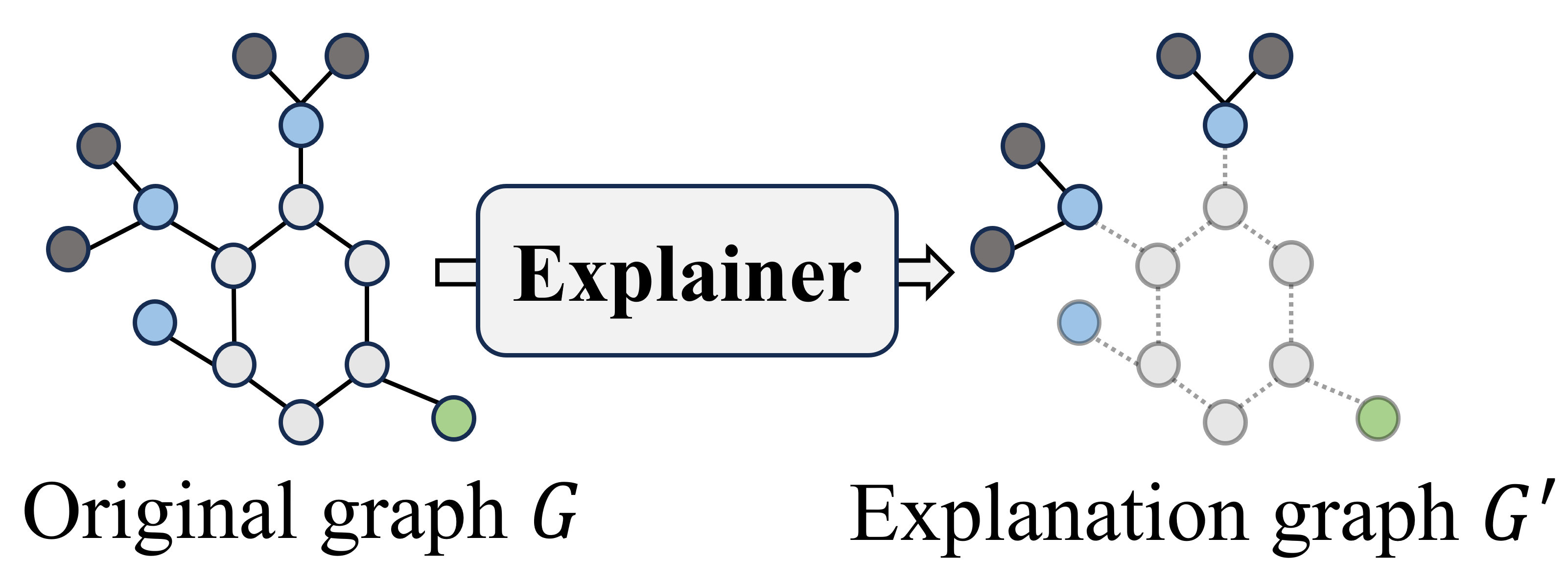
((a)) Explanation process

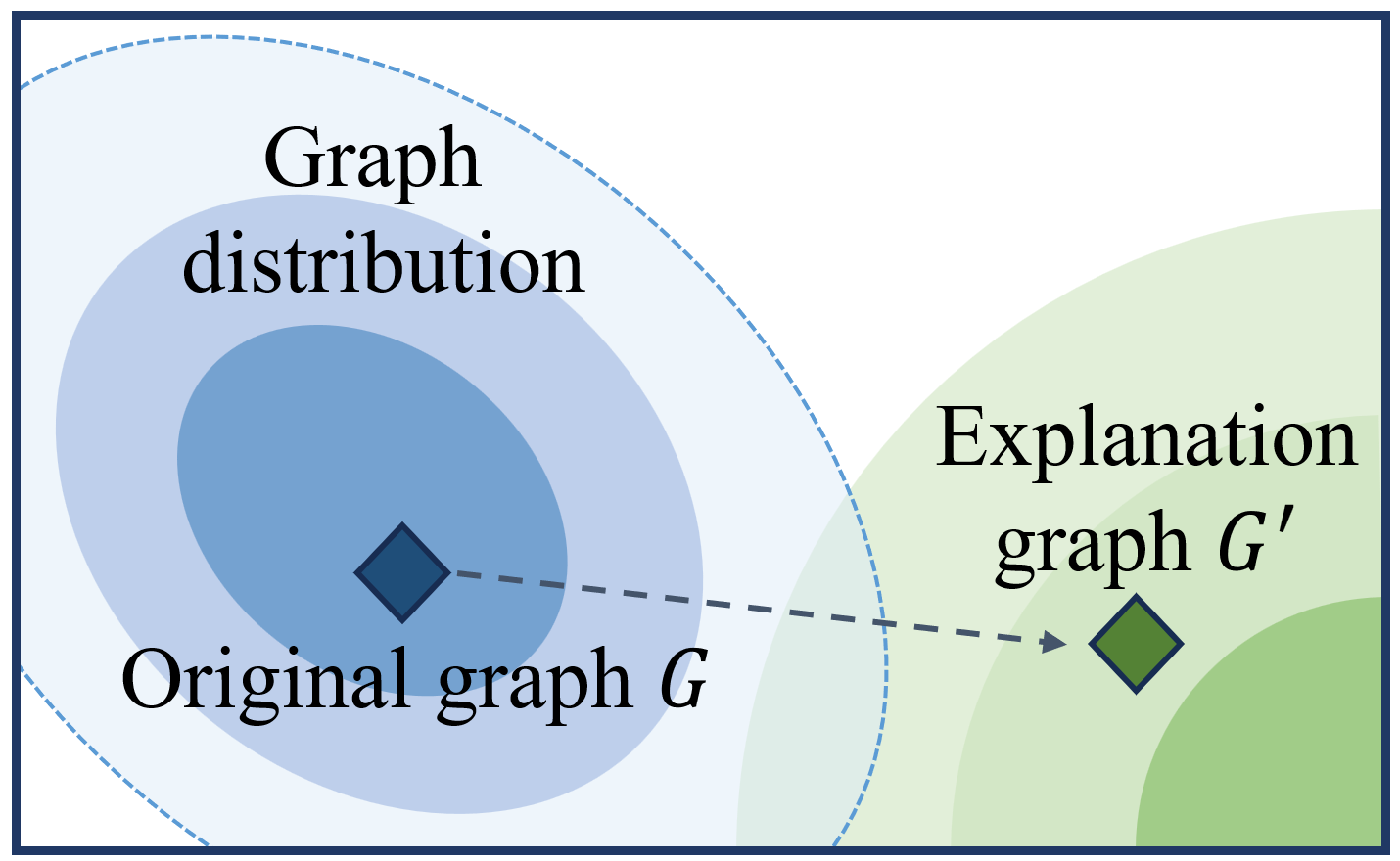
((b)) OOD problem

Figure 1: Examples of the explanation process and out-of-distribution problem. (a) is the explanation process for a graph learning model. The original graph $G$ undergoes an explanation process, resulting in an explanation graph $G^{\prime}$ that highlights the most significant features and relationships; (b) shows the explanation graph $G^{\prime}$ is out of distribution where the GNN is well-trained.

Although it is intuitively correct, the underlying assumption of the aforementioned approach – GNN model can make accurate predictions on explanation subgraphs – may not always hold. Prior research indicates that explanation subgraphs can significantly deviate from the distribution of original graphs, leading to an Out-Of-Distribution (OOD) issue (Zhang et al., 2023b; Fang et al., 2023d, b). For instance, in the MUTAG dataset (Debnath et al., 1991), each graph represents a molecule, with nodes symbolizing atoms and edges indicating chemical bonds. The molecular graphs in this dataset usually contain hundreds of edges. In contrast, the $NO_{2}$ functional group, identified as a key subgraph influencing positive mutagenicity in a molecule, comprises merely 2 edges. This stark contrast in structural properties leads to a significant difference in the distributions of explanation subgraphs and original graphs. Since the model was trained with original graphs, the reliability of predictions on subgraphs is undermined due to the distribution shifting problem.

Several pioneering studies have attempted to address this distributional challenge (Fang et al., 2023d; Zhang et al., 2023b, a). For example, CGE regards the GNN model as a transparent, fully accessible system. It considers the GNN model as a teacher network and employs an additional “student” network to predict the labels of explanation subgraphs (Fang et al., 2023d). As another example, MixupExplainer (Zhang et al., 2023b) generates a mixed graph for the explanation by blending it with a non-explanatory subgraph from a different input graph. This method posits that the mixup graph aligns with the distribution of the original input graphs. However, this claim is predicated on a rather simplistic assumption that the explanation and non-explanatory subgraphs are independently drawn. However, in real-world applications, these methods often face practical limitations. The dependence on a “white box” model in CGE and the oversimplified assumptions in MixupExplainer are not universally applicable. Instead, GNN models are usually given as “black boxes”, and the graphs in real-life applications do not conform to strict independence constraints, highlighting the need for more versatile and realistic approaches to the OOD problem.

In response to these challenges, in this work, we introduce an innovative concept of proxy graphs to the realm of explainable GNNs. These proxy graphs are designed to be both explanation-preserving and distributionally aligned with the training data. By this means, the predictive capabilities of explanation subgraphs can be reliably inferred from the corresponding proxy graphs. We begin with a thorough investigation into the feasible conditions necessary for generating such in-distributed proxy graphs. Leveraging our findings, we further propose a novel architecture that incorporates variational graph auto-encoders to produce proxy graphs. Specifically, we utilize a graph auto-encoder to reconstruct the explainable subgraph and another variational auto-encoder to generate a non-explanatory subgraph. A proxy graph is then obtained by combining two output subgraphs of auto-encoders. We delineate our main contributions as follows:

• We systematically analyze and address the challenge of the out-of-distribution issue in explainable GNNs, which is pivotal for enhancing the reliability and interpretability of GNNs in real-world applications.

• We introduce an innovative parametric method that incorporates graph auto-encoders to produce in-distributed proxy graphs that are both situated in the original data distribution and preserve essential explanation information. This facilitates more precise and interpretable explanations in GNN applications.

• Through comprehensive experimentation and rigorous evaluations on various real-world datasets, we substantiate the effectiveness of our proposed approach, showcasing its practical utility and superiority in producing explanations.

2 Notations and Preliminary

2.1 Notations and Problem Formulation.

We denote a graph $G$ from an alphabet ${\mathcal{G}}$ by a triple $({\mathcal{V}},{\mathcal{E}};{\bm{X}})$, where ${\mathcal{V}}=\{v_{1},v_{2},...,v_{n}\}$ is the node set and ${\mathcal{E}}\subseteq{\mathcal{V}}\times{\mathcal{V}}$ is the edge set. ${\bm{X}}\in{\mathbb{R}}^{n\times d}$ is the node feature matrix, where $d$ is the feature dimension and the $i$-th row is the feature vector associated with node $v_{i}$. The adjacency matrix of $G$ is denoted by ${\bm{A}}\in\{0,1\}^{n\times n}$, which is determined by the edge set $\mathcal{E}$ that ${A}_{ij}=1$ if $(v_{i},v_{j})\in\mathcal{E}$, ${A}_{ij}=0$, otherwise. In this paper, we focus on the graph classification task, as the node classification can be converted to computation graph classification problem (Ying et al., 2019; Luo et al., 2020). Specifically, for the graph classification task, each graph $G$ is associated with a label $Y\in\mathcal{C}$. The to-be-explained GNN model $f(\cdot)$ has been well-trained to classify $G$ into its class, i.e., $f:{\mathcal{G}}\mapsto\{1,2,\cdots,|\mathcal{C}|\}$.

Following existing works (Yuan et al., 2022; Luo et al., 2020; Ying et al., 2019), the explanation methods under consideration in this paper are model/task agnostic and treat GNN models as black boxes — i.e., the so-called post-hoc, instance-level explanation methods. Formally, our research problem is described as follows (Huang et al., 2024):

Problem 1 (Post-hoc Instance-level GNN Explanation).

Given a to-be-explained GNN model $f(\cdot)$ and a set of graphs ${\mathcal{G}}$, the goal of post-hoc instance-level explanation is to learn a parametric function that for an arbitrary graph $G\in{\mathcal{G}}$, it finds a compact subgraph $G^{*}\subseteq G$ that can “explain” the prediction $f(G)$. The parametric mapping $\Psi_{\psi}:{\mathcal{G}}\mapsto{\mathcal{G}}^{*}$ is called an explanation function, where ${\mathcal{G}}^{*}$ is the alphabet of $G^{*}$, and $\psi$ is the parameter of the explanation function.

2.2 Graph Information Bottleneck as the Objective Function.

The Information Bottleneck (IB) principle, foundational in learning dense representations, suggests that optimal representations should balance minimal and sufficient information for predictions (Tishby et al., 2000). This concept has been adapted for GNNs through the Graph Information Bottleneck (GIB) approach, consolidating various post-hoc GNN explanation methods like GNNExplainer (Ying et al., 2019) and PGExplainer (Luo et al., 2020). The GIB framework aim to find a subgraph $G^{*}$ to explain the GNN model’s prediction on a graph $G$ as (Zhang et al., 2023b):

$$G^{*}=\operatorname*{arg\,min}_{G^{\prime}}I(G,G^{\prime})-\alpha I(Y,G^{\prime}),$$ (1)

where $G^{\prime}$ is a candidate explanatory subgraph, $Y$ is the label, and $\alpha$ is a balance parameter. The first term is the mutual information between the original graph $G$ and the explanatory subgraph $G^{\prime}$ and the second term is negative mutual information of $Y$ and the explanation subgraph $G^{\prime}$. At a high level, the first term encourages detecting a small and dense subgraph for explanation, and the second term requires that the explanation subgraph is label preserving.

Due to the intractability of mutual information between $Y$ and $G^{\prime}$ in equation 1, existing works (Miao et al., 2022; Wu et al., 2020) derive a parameterized variational lower bound of $I(Y,G^{\prime})$:

$$I(Y,G^{\prime})\geq\mathbb{E}_{G^{\prime},Y}[\log P(Y|G^{\prime})]+H(Y),$$ (2)

where the first term measures how well the subgraphs predict the labels. A higher value indicates that the subgraphs are, on average, more predictive of the correct labels. The second term $H(Y)$ quantifies the amount of inherent unpredictability or variability in the labels. By introducing equation 2 to equation 1, a tractable upper bound is used as the objective:

$$G^{*}=\operatorname*{arg\,min}_{G^{\prime}}{I(G,G^{\prime})-\alpha\mathbb{E}_{G^{\prime},Y}[\log P(Y|G^{\prime})]},$$ (3)

where $H(Y)$ is omitted due to its independence to $G^{\prime}$.

The OOD Problem in GIB. In existing research, the estimation of $P(Y|G^{\prime})$ is typically achieved by applying the to-be-explained model $f$, to the input graph $G^{\prime}$ (Ying et al., 2019; Miao et al., 2022). A critical assumption in existing approaches involves the GNN model’s ability to accurately predict candidate explanation subgraphs $G^{\prime}$. This assumption, however, often overlooks the OOD problem, where the distribution of explanation subgraphs significantly deviates from that of the original training graphs (Zhang et al., 2023b; Fang et al., 2023a). Formally, let $P_{\mathcal{G}}$ denote the distribution of training graphs, and $P_{{\mathcal{G}}^{\prime}}$ represents the distribution of explanation subgraphs. The core issue in the GIB objective function is caused by $P_{\mathcal{G}}\neq P_{{\mathcal{G}}^{\prime}}$. This distributional disparity undermines the predictive reliability of the model $f(\cdot)$, trained on $P_{\mathcal{G}}$ when applied to subgraphs from $P_{{\mathcal{G}}^{\prime}}$. As a result, the predictive power of explanations provided by $f(G^{\prime})$ is unreliable approximation of $P(Y|G^{\prime})$ in  equation 3.

3 Graph Information Bottleneck with Proxy Graphs

In this section, we propose the concept of a proxy graph to mitigate the above-mentioned OOD issue. This proxy graph not only retains the label information present in $G^{\prime}$ but also conforms to the distribution of the original graph dataset. Specifically, we assume that proxy graphs $\tilde{G}$ are drawn from a distribution $P_{\mathcal{G}}$ and reformulate the estimation of $P(Y|G^{\prime})$ by marginalizing over the distribution of proxy graphs as follows.

$$P(Y|G^{\prime})=\mathbb{E}_{\tilde{G}\sim P_{\mathcal{G}}}[P(Y|\tilde{G})\cdot P(\tilde{G}|G^{\prime})]$$ (4)

In equation 4, we address the OOD challenge by predicting $Y$ using a proxy graph $\tilde{G}$ instead of directly using $G^{\prime}$. This approach is particularly effective when the conditional probability $P(Y|\cdot)$ is approximated by the model $f(\cdot)$. To facilitate the maximization of the likelihood as outlined in equation 4, we further approximate $P(\tilde{G}|G^{\prime})$ with a parameterized function, denoted as $Q_{\bm{\phi}}(\tilde{G}|G^{\prime})$. The formal representation is thus given by

$$P(Y|G^{\prime})=\mathbb{E}_{\tilde{G}\sim P_{\mathcal{G}}}[P(Y|\tilde{G})\cdot Q_{\bm{\phi}}(\tilde{G}|G^{\prime})],$$ (5)

where $\bm{\phi}$ denotes model parameters.

Given the combinatorial complexity inherent in graph structures, it is computationally infeasible to enumerate all potential proxy graphs $\tilde{G}$ from the unknown distribution $P_{\mathcal{G}}$, which is necessary for calculating equation 5. To overcome this challenge, we propose approximating $P_{\mathcal{G}}$ with the parameterized function $Q_{\bm{\phi}}(\tilde{G}|G^{\prime})$. Consequently, we estimate equation 5 by sampling proxy graphs from $Q_{\bm{\phi}}(\tilde{G}|G^{\prime})$, leading to the following formulation:

$$P(Y|G^{\prime})=\mathbb{E}_{\tilde{G}\sim Q_{\bm{\phi}}(\tilde{G}|G^{\prime})}[P(Y|\tilde{G})],$$ (6)

with constraints

$$Q_{\bm{\phi}}(\tilde{G}|G^{\prime})\approx P_{\mathcal{G}},\quad H(Y|\tilde{G})\approx H(Y|G^{\prime}),$$ (7)

The first constraint ensures that $\tilde{G}$ is sampled from a distribution that approximates $P_{\mathcal{G}}$, effectively addressing the OOD challenge. The second constraint guarantees that the label information preserved in $\tilde{G}$ is similar to that in $G^{\prime}$. Therefore, our proxy graph-induced objective function becomes:

$$\operatorname*{arg\,min}_{G^{\prime}}{I(G,G^{\prime})-\alpha\mathbb{E}_{G^{\prime},Y}[\log\mathbb{E}_{\tilde{G}\sim Q_{\bm{\phi}}(\tilde{G}|G^{\prime})}[P(Y|\tilde{G})]]}$$ (8)

$$\text{s.t.}~{}~{}~{}Q_{\bm{\phi}}(\tilde{G}|G^{\prime})\approx P_{\mathcal{G}},~{}~{}~{}H(Y|\tilde{G})\approx H(Y|G^{\prime})$$

Bi-level optimization In equation 8, we formulate a joint optimization loss function that aims to identify the optimal explanation alongside its corresponding proxy graphs. Building upon this, we refine the framework by replacing the first constraint with a distributional distance measure, specifically the Kullback-Leibler (KL) divergence, between $Q_{\bm{\phi}}(\tilde{G}|G^{\prime})$ and $P_{\mathcal{G}}$. This leads to the development of a bi-level optimization model. Formally, the model is expressed as follows:

$$\operatorname*{arg\,min}_{G^{\prime}}{I(G,G^{\prime})-\alpha\mathbb{E}_{G^{\prime},Y}[\log\mathbb{E}_{\tilde{G}\sim Q_{\bm{\phi}^{*}}(\tilde{G}|G^{\prime})}[P(Y|\tilde{G}^{*})]]}$$ (9)

$$\quad\text{where }\bm{\phi}^{*}=\operatorname*{arg\,min}_{\bm{\phi}}{\text{KL}(Q_{\bm{\phi}}(\tilde{G}|G^{\prime}),P_{\mathcal{G}})},$$

$$\quad\quad\quad\text{s. t. }H(Y|\tilde{G})\approx H(Y|G^{\prime}).$$

3.1 Derivation of Outer Optimization

For the outer optimization objective, we elaborate on operationalizing $I(G,G^{\prime})$. Akin to the original graph, We denote the explanation subgraph $G^{\prime}$ by $({\mathcal{V}},{\mathcal{E}}^{\prime},{\bm{X}})$, whose adjacency matrix is ${\bm{A}}^{\prime}$. We follow (Miao et al., 2022) to include a variational approximation distribution $R(G^{\prime})$ for the distribution $P(G^{\prime})$. Then, we obtain its upper bounds as follows.

$$I(G,G^{\prime})\leq\mathbb{E}_{G}[\text{KL}(P(G^{\prime}|G)||R(G^{\prime}))]$$ (10)

We follow the Erdős–Rényi model (Erdős et al., 1960) and assume that each edge in $G^{\prime}$ has a probability of being present or absent, independently of the other edges. Specifically, we assume that the existence of an edge $(u,v)$ in $G^{\prime}$ is determined by a Bernoulli variable $A_{u,v}^{\prime}\sim\text{Bern}(\pi_{uv})$. Thus, $P(G^{\prime}|G)$ can be decompose with $P(G^{\prime}|G)=\prod_{(u,v)\in{\mathcal{E}}}P(A_{uv}^{\prime}|\pi_{uv})$. The bound is always true for any prior distribution $R(G^{\prime})$. We follow an existing work and assume that in prior distribution, the existence of an edge $(u,v)$ in $G^{\prime}$ is determined by another Bernoulli variable $A^{{}^{\prime\prime}}_{u,v}\sim\text{Bern}(r)$, where $r\in[0,1]$ is a hyper-parameter (Miao et al., 2022), independently to the graph $G$. We have $R(G^{\prime})=P(|{\mathcal{E}}|)\prod_{(u,v)\in{\mathcal{E}}}P(A^{{}^{\prime\prime}}_{uv})$. Thus, the KL divergence between $P(G^{\prime}|G)$ and the above marginal distribution $R(G^{\prime})$ becomes:

$$\text{KL}(P(G^{\prime}|G)||R(G^{\prime}))$$ (11)

$$= \sum_{(u,v)\in{\mathcal{E}}}\pi_{uv}\log\frac{\pi_{uv}}{r}+(1-\pi_{uv})\log\frac{1-\pi_{uv}}{1-r}+\text{Const}.$$

By replacing $I(G^{\prime}G^{\prime})$ with the above tractable upper bound, we obtain the loss function, denoted by $\mathcal{L}_{\text{exp}}$, to train the explainer $\Psi(\cdot)$.

3.2 Derivation of Inner Optimization

For the inner optimization objective, we implement the first constraint by minimizing the distribution distance between $Q_{\bm{\phi}}(\tilde{G}|G^{\prime})$ and $P_{\mathcal{G}}$, under the Erdős–Rényi assumption, the distribution loss is equivalent to the cross-entropy loss between $\tilde{G}$ given $G^{\prime}$ and $G$ over the full adjacency matrix (Chen et al., 2023). Considering that $G$ is usually sparse compared to a fully connected graph, in practice, we adopt a weighted version to emphasize more connected node pairs (Wang et al., 2016). Formally, we have the following distribution loss.

$${\mathcal{L}}_{\text{dist}}=\frac{\beta}{|{\mathcal{E}}|}\sum_{(u,v)\in{\mathcal{E}}}\log(\tilde{p}_{uv})+\frac{1}{|\bar{{\mathcal{E}}}|}\sum_{(u,v)\in\bar{{\mathcal{E}}}}\log(1-\tilde{p}_{uv}),$$ (12)

where $\bar{{\mathcal{E}}}$ is the set of node pairs that are unconnected in $G$, $\tilde{p}_{uv}$ is the probability of node pair $(u,v)$ in $\tilde{G}$, and $\beta$ is a hyper-parameter to get a trade-off between connected and unconnected node pairs.

The second constraint requires the mutual information of $Y$ and $\tilde{G}$ is the same as that of $Y$ and $G^{\prime}$. Due to the OOD problem, it is non-trivial to directly compute $P(Y|G^{\prime})$ or $H(Y|G^{\prime})$. Instead, we implement this constraint with a novel graph generator that $\tilde{G}$ is obtained by combining $G^{\prime}$ and a non-explanatory subgraph (Zhang et al., 2023b). In practice, we implement the non-explanatory part by perturbing the remaining subgraph $G-G^{\prime}$. The intuition is that if an explanation comprises information, it is hard to change the prediction by manipulating the remaining part that is non-explanatory, which is widely adopted in the literature (Fang et al., 2023a; Zhang et al., 2023b; Zheng et al., 2023).

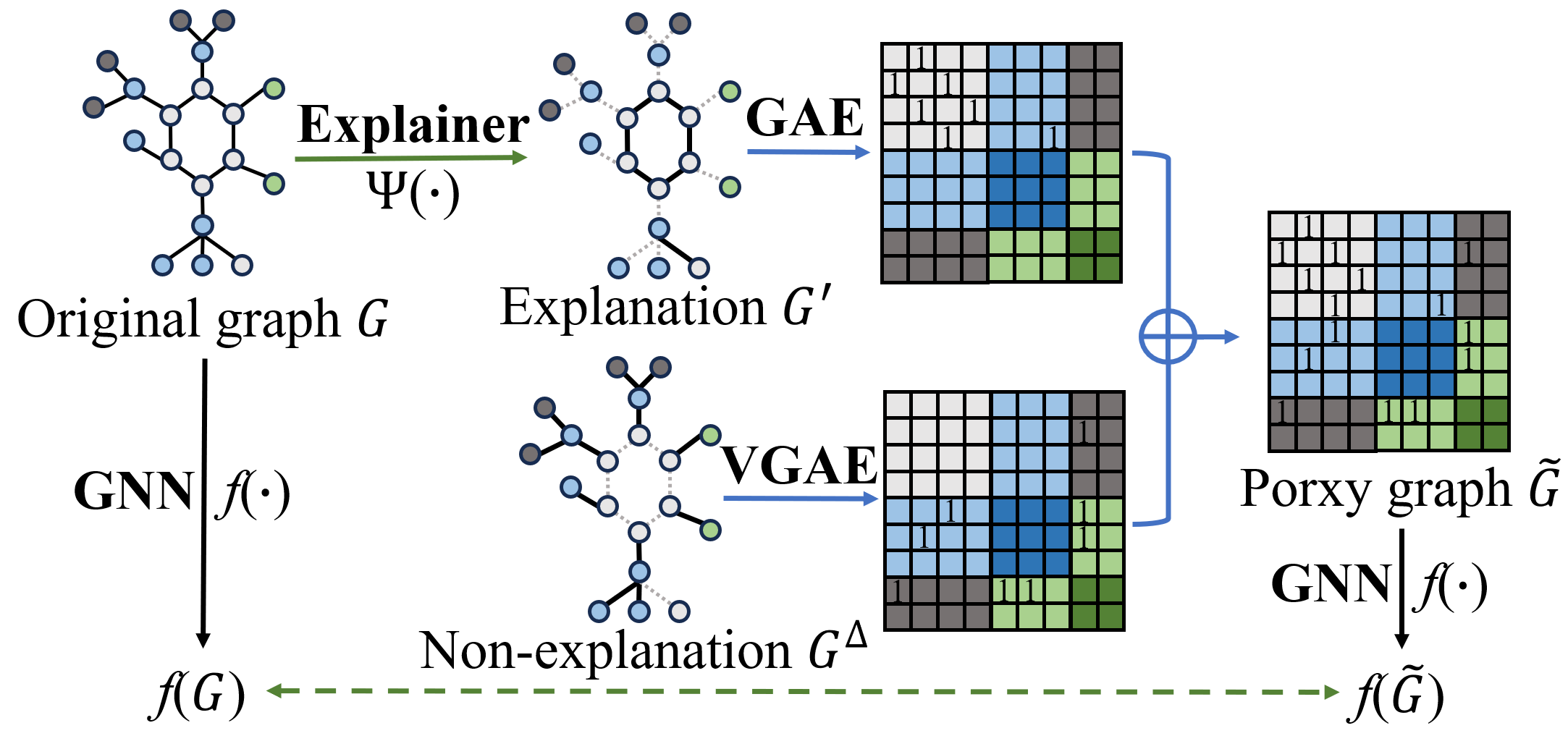
Figure 2: ProxyExplainer consists of two components: an Explainer and a Proxy Graph Generator. The Explainer takes a graph $G$ as input and produces an explainable subgraph $G^{\prime}$, The proxy generator creates an in-distribution proxy graphs that preserve the label information in $G^{\prime}$. The proxy generator consists of a graph auto-encoder (GAE) and a variational graph auto-encoder (VGAE).

4 The ProxyExplainer

Inspired by our novel GIB with proxy graphs, in this section, we introduce a straightforward yet theoretically robust instantiation, named ProxyExplainer. As shown in Figure 2, the architecture of our model comprises two key modules: the explainer and the proxy graph generator. The explainer takes the $G$ as input and outputs a subgraph $G^{\prime}$ as an explanation, which is optimized through the outer objective in equation 9. The proxy graph generator generates an in-distributed proxy graph, which is optimized with the inner objective.

4.1 The Explainer

For the sake of optimization, we follow existing works to relax the element in ${\bm{A}}$ from binary values to continuous values in the range $[0,1]$ (Ying et al., 2019; Luo et al., 2020; Miao et al., 2022). We adopt a generative explainer due to its effectiveness and efficiency (Luo et al., 2020). Specifically, we decompose the to-be-explained model $f(\cdot)$ into two functions that $f_{\text{enc}}(\cdot)$ learns node representations and $f_{\text{cls}}(\cdot)$ predicts graph labels based on node embeddings. Formally, we have ${\bm{Z}}=f_{\text{enc}}({\bm{X}},{\bm{A}})$ and $Y=f_{\text{cls}}({\bm{Z}})$, where ${\bm{Z}}\in{\mathbb{R}}^{N\times F}$ is the node representation matrix and $F$ is the number of feature dimenions. Routinely, $f_{\text{cls}}(\cdot)$ consists of a pooling layer followed by a classification layer and $f_{\text{enc}}(\cdot)$ consists of the other layers. Following the independence assumption in Section 3.1, we approximate Bernoulli distributions with binary concrete distributions (Maddison et al., 2017; Jang et al., 2017). Specifically, the probability of sampling an edge $(i,j)$ is computed by an MLP parameterized by $\psi$, denoted by $g_{\psi}(\cdot)$. Formally, we have

$$\omega_{ij}=g_{\psi}([{\bm{z}}_{i};{\bm{z}}_{j}]),\quad\quad\epsilon\sim\text{Uniform}(0,1)$$ (13)

$${A}_{ij}^{\prime}=\sigma((\log\epsilon-\log(1-\epsilon)+\omega_{ij})/\tau),$$

where $[{\bm{z}}_{i};{\bm{z}}_{j}]$ is the concatenation of node representations ${\bm{z}}_{i}$ and ${\bm{z}}_{j}$, $\epsilon$ is a independent variable, $\sigma(\cdot)$ is the Sigmoid function, and $\tau$ is a temperature hyper-parameter for approximation.

4.2 The Proxy Graph Generator

As shown in our analysis in Section 3.2, we demonstrate the synthesis of a proxy graph through the amalgamation of the explanation subgraph $G^{\prime}$ and the perturbation of its non-explanatory subgraph, represented as $G^{\Delta}=({\mathcal{V}},{\mathcal{E}}^{\Delta},{\bm{X}})$. We define the edge set of $G^{\Delta},{\mathcal{E}}^{\Delta}$, as the differential set ${\mathcal{E}}-{\mathcal{E}}^{\prime}$. Correspondingly, the adjacency matrix ${\bm{A}}^{\Delta}$ is derived through ${\bm{A}}-{\bm{A}}^{\prime}$. Building upon this foundation, and as illustrated in Figure 2, our proposed framework introduces a dual-structured mechanism comprising two distinct graph auto-encoders(GAE) (Bank et al., 2023). To be more specific, we first include an encoder to learn a latent matrix ${\bm{Z}}^{\prime}$ according to ${\bm{A}}^{\prime}$ and ${\bm{X}}^{\prime}$, and a decoder network recovers ${\bm{A}}^{\prime}$ based on ${\bm{Z}}^{\prime}$. Formally, we have:

$${\bm{Z}}^{\prime}=\text{ENC}_{1}({\bm{A}}^{\prime},{\bm{X}}),\quad\tilde{{\bm{A}}}^{\prime}=\text{DEC}({\bm{Z}}^{\prime}),$$ (14)

where $\text{ENC}_{1}$ and DEC are the encoder network and decoder network. Our framework is flexible to the choices of these two networks. $\tilde{{\bm{A}}}^{\prime}\in{\mathbb{R}}^{n\times n}$ is the reconstructed adjacency matrix.

To introduce perturbations into the non-explanatory segment, our approach employs a Variational Graph Auto-Encoder (VGAE), a generative model adept at creating varied yet structurally coherent graph data. This capability is pivotal in generating nuanced variations of the non-explanatory subgraph. The VGAE operates by first encoding the non-explanatory subgraph $G^{\Delta}$ into a latent probabilistic space, characterized by Gaussian distributions. This process is articulated as:

$$\bm{\mu}^{\Delta}=\text{ENC}_{1}({\bm{A}}^{\Delta},{\bm{X}}),\quad\bm{\sigma}^{\Delta}=\text{ENC}_{2}({\bm{A}}^{\Delta},{\bm{X}}),$$ (15)

where $\text{ENC}_{1}$ and $\text{ENC}_{2}$ are encoder networks that learn the mean $\bm{\mu}^{\Delta}$ and variance $\bm{\sigma}^{\Delta}$ of the Gaussian distributions, respectively. Following this, the latent representations ${\bm{Z}}^{\Delta}$ are sampled from these distributions, ensuring that each generated instance is a unique variation of the original. The decoder network then reconstructs the perturbed non-explanatory subgraph from these sampled latent representations:

$${\bm{Z}}^{\Delta}\sim\mathcal{N}(\bm{\mu}^{\Delta},\text{diag}(\bm{\sigma}^{\Delta})^{2}),\quad\tilde{{\bm{A}}}^{\Delta}=\text{DEC}({\bm{Z}}^{\Delta}),$$ (16)

where $\tilde{{\bm{A}}}^{\Delta}\in{\mathbb{R}}^{n\times n}$ represents the adjacency matrix of the perturbed non-explanatory subgraph. This novel use of VGAE facilitates the generation of diverse yet representative perturbations, crucial for enhancing the interpretability of explainers in our proxy graph framework. The adjacency matrix of a proxy graph is then obtained by

$$\tilde{{\bm{A}}}=\tilde{{\bm{A}}}^{\prime}+\tilde{{\bm{A}}}^{\Delta}.$$ (17)

Table 1: Explanation accuracy in terms of AUC-ROC on edges under six datasets based on GCN.

	BA-2motifs	BA-3motifs	Alkane-Carbonyl	Benzene	Fluoride-Carbonyl	MUTAG
GradCAM	0.714±0.000	0.709±0.000	0.496±0.000	0.662±0.000	0.604±0.000	0.573±0.000
GNNExplainer	0.644±0.007	0.511±0.002	0.532±0.008	0.499±0.004	0.540±0.002	0.682±0.009
PGExplainer	0.734±0.117	0.796±0.010	0.611±0.071	0.698±0.099	0.591±0.041	0.832±0.032
ReFine	0.698±0.001	0.629±0.005	0.630±0.007	0.533±0.011	0.507±0.003	0.612±0.004
MixupExplainer	0.906±0.059	0.859±0.019	0.642±0.033	0.520±0.043	0.534±0.012	0.883±0.103
ProxyExplainer	0.935±0.008	0.960±0.008	0.806±0.003	0.745±0.012	0.641±0.070	0.977±0.009

Loss function. To train the proxy graph generator, we introduce a standard Gaussian distribution as the prior for the latent space representations in the VGAE, specifically ${\bm{Z}}\sim\mathcal{N}(0,\mathcal{I})$, where $\mathcal{I}$ represents the identity matrix. Then, the loss function is as follows.

$$\mathcal{L}_{\text{proxy}}=\mathcal{L}_{\text{dist}}+\lambda\mathcal{L}_{\text{KL}},$$ (18)

where $\mathcal{L}_{\text{dist}}$ is the distribution distance between $\tilde{G}$ and $G$. $\mathcal{L}_{\text{KL}}$ represents the Kullback-Leibler (KL) divergence between the distribution of the latent representations ${\bm{Z}}^{\Delta}$ and the assumed Gaussian prior. This term is crucial for regulating the variational aspect of the VGAE, ensuring that the generated perturbations are meaningful and controlled. $\lambda$ is the hyper-parameter.

Alternative Training. To train explainer and proxy graph generator networks, we follow existing works (Zheng et al., 2023) to use an alternating training schedule that trains the proxy graph generator network $M$ times and then trains the explainer network one time. $M$ is a hyper-parameter determined by grid search. The detailed algorithm description of our model is shown in Appendix B.

5 Related Work

GNN Explanation. The goal of explainability in GNNs is to ensure transparency in graph-based tasks. Recent works have been directed towards elucidating the rationale behind GNN predictions. These explanation methods can be broadly classified into two categories: instance-level and model-level approaches (Yuan et al., 2022). In this study, we focus on instance-level explanations, which aim to clarify the specific reasoning behind individual predictions made by GNNs. These methods are critical for understanding the decision-making process on a case-by-case basis to enhance the explainability of GNNs in graph classification tasks. For example, GNNExplainer (Ying et al., 2019) excludes certain edges and node features to observe the changes in classification. However, its single-instance focus limits its applicability to provide a global understanding of the to-be-explained model. PGExplainer (Luo et al., 2020) introduces a parametric neural network to learn edge weights. Thus, once training is complete, it can explain new graphs without retraining. ReFine (Wang et al., 2021) integrates a pre-training phase that focuses on class comparisons and is fine-tuned to refine context-specific explanations. GStarX (Zhang et al., 2022b) assigns an importance score to each node by caculating the Hamiache and Navarro values of the structure to obtain explanatory subgraphs. GFlowExplainer (Li et al., 2023) uses a generator to construct a TD-like flow matching condition to learn a policy for generating explanations by adding nodes sequentially.

Distribution Shifting in Explanations. The distribution shifting problem in post-hoc explanations has been increasingly recognized in explainable AI fields (Chang et al., 2019; Qiu et al., 2022). For example, FIDO (Chang et al., 2019) works on enhancing image classifier explanations, focusing on relevant contextual details that agree with the training data’s distribution. A recent study tackles the distribution shifting problem in image explanations by introducing a module that assesses the similarity between altered data and the original dataset distribution (Qiu et al., 2022). In the graph domain, an ad-hoc strategy to mitigate distribution shifting is to initially reduce the size constraint coefficient during the explanation process (Fang et al., 2023c). MixupExplainer (Zhang et al., 2023b) proposes a non-parametric solution by mixing up the explanation subgraph with a non-explainable part from another graph. However, this method operates under the assumption that the explanatory and non-explanatory subgraphs in mixed graphs are independent, which may not hold in many real-life graphs.

6 Experiments

We present empirical results that illustrate the effectiveness of our proposed method. These experiments are mainly designed to explore the following research questions:

• RQ1: Can the proposed framework outperform other baselines in identifying explanations for GNNs?

• RQ2: Is the distribution shifting severe in explanation subgraphs? Can the proposed approach alleviate that?

• RQ3: How does each component of ProxyExplainer impact the overall performance in generating explanations?

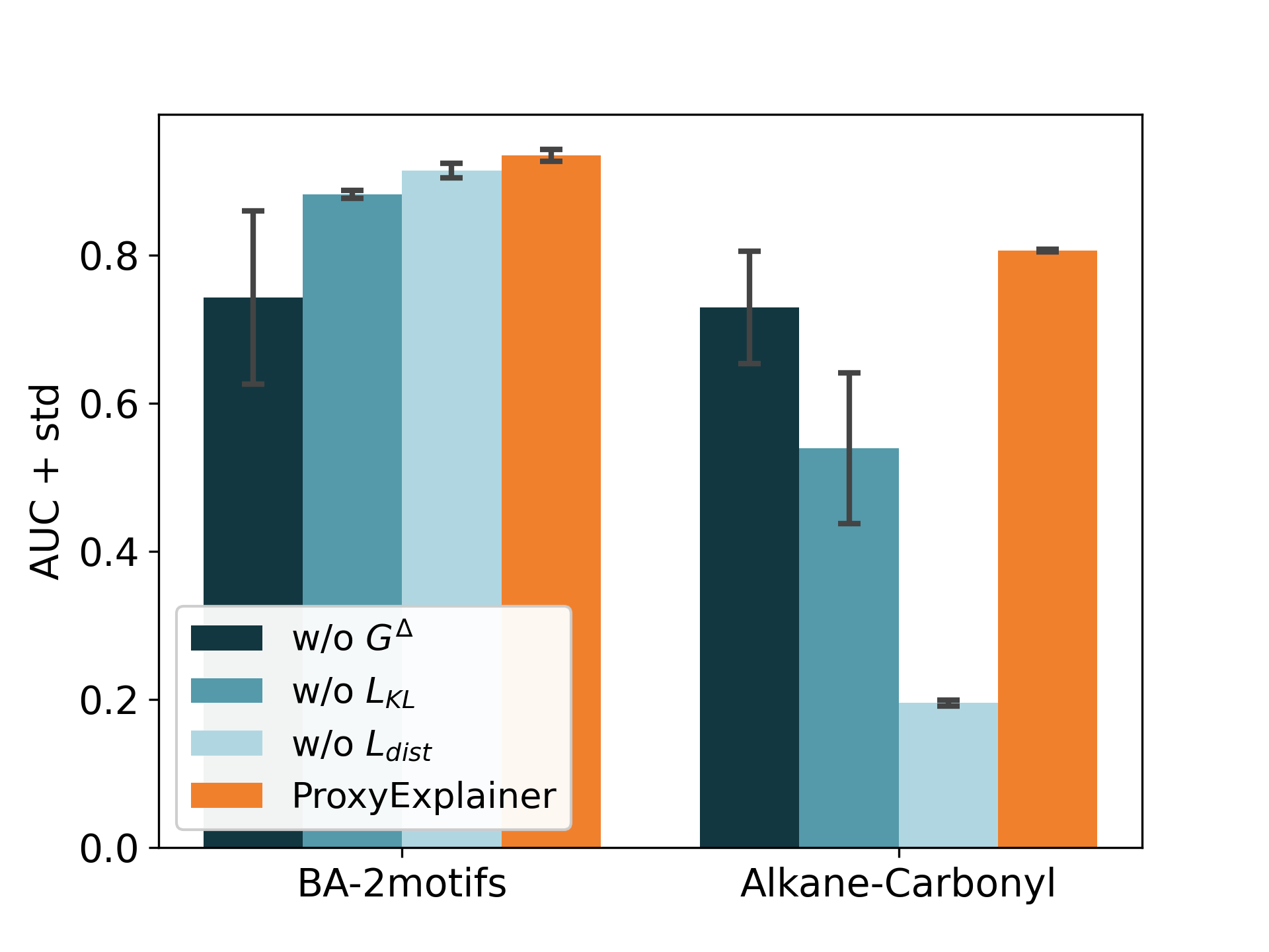
Figure 3: Ablation Studies on BA-2motifs and Alkane-Carbonyl.

6.1 Experimental Settings

To evaluate the performance of ProxyExplainer, we use six benchmark datasets with ground-truth explanations. These include two synthetic datasets: BA-2motifs (Luo et al., 2020) and BA-3motifs (Chen et al., 2023), along with four real-world datasets: Alkane-Carbonyl (Sanchez-Lengeling et al., 2020), Benzene (Sanchez-Lengeling et al., 2020), Fluoride-Carbonyl (Sanchez-Lengeling et al., 2020), and MUTAG (Kazius et al., 2005). We take GradCAM (Pope et al., 2019), GNNExplainer(Ying et al., 2019), PGExplainer(Luo et al., 2020), ReFine (Wang et al., 2021), and MixupExplainer (Zhang et al., 2023b) for comparison. We follow the experimental setting in previous works (Ying et al., 2019; Luo et al., 2020; Sanchez-Lengeling et al., 2020) to train a Graph Convolutional Network (GCN) model with three layers. We use the Adam optimizer (Kingma & Ba, 2014) with the inclusion of a weight decay $5e-4$. To evaluate the quality of explanations, we approach the explanation task as a binary classification of edges. Edges that are part of ground truth subgraphs are labeled as positive, while all others are deemed negative. The importance weights given by the explanation methods are interpreted as prediction scores. An effective explanation technique is one that assigns higher weights to edges within the ground truth subgraphs compared to those outside of them. For quantitative assessment, we utilize the AUC-ROC metric. Detailed information regarding datasets and baselines is delineated in the Appendix C.

6.2 Quantitative Evaluation (RQ1)

To answer RQ1, we compare the proposed method, ProxyExplainer, to other baselines. Each experiment was conducted 10 times using random seeds, and the average AUC scores as well as standard deviations are presented in Table 1.

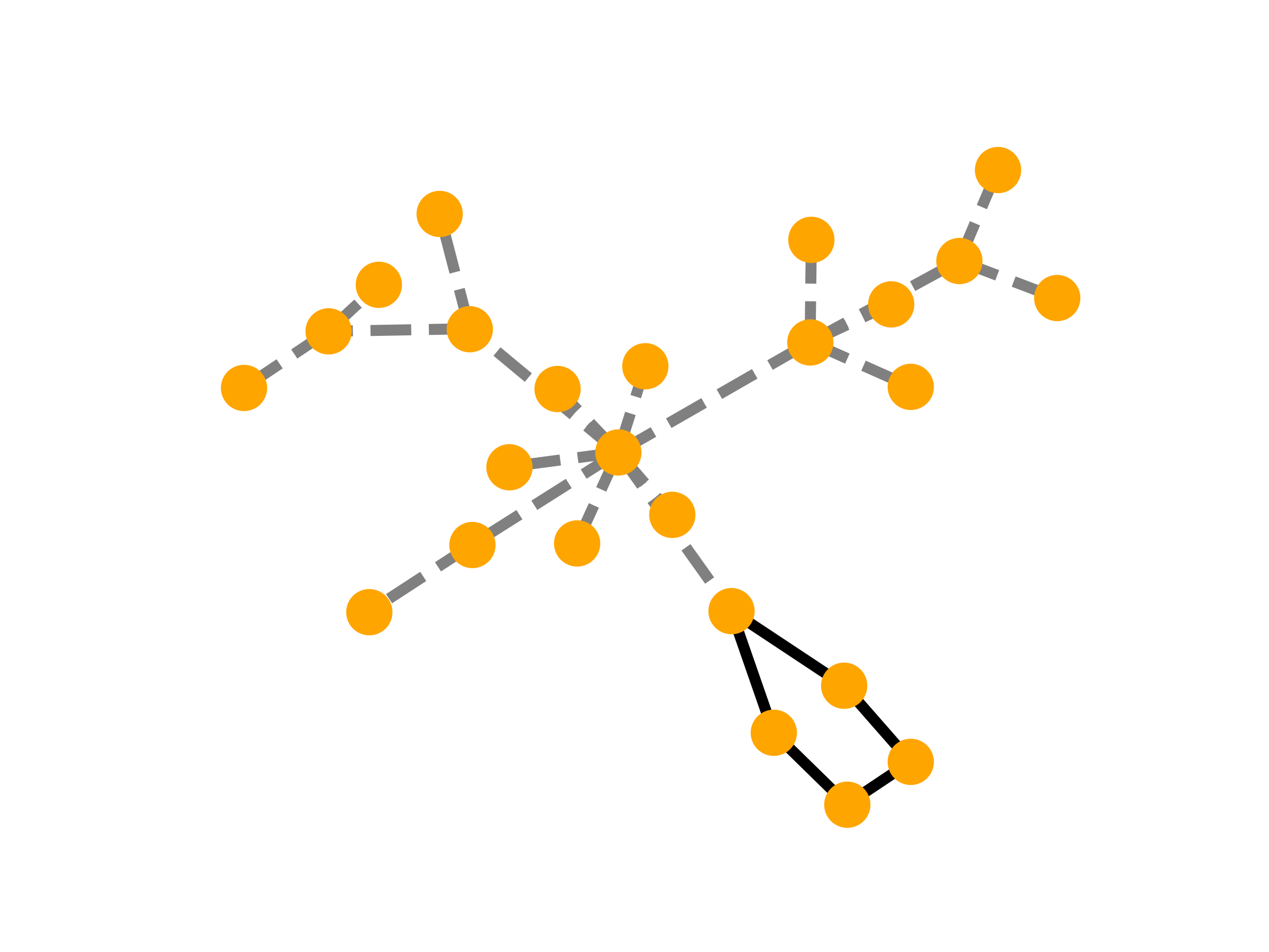
((a)) Ground Truth

((b)) ProxyExplainer

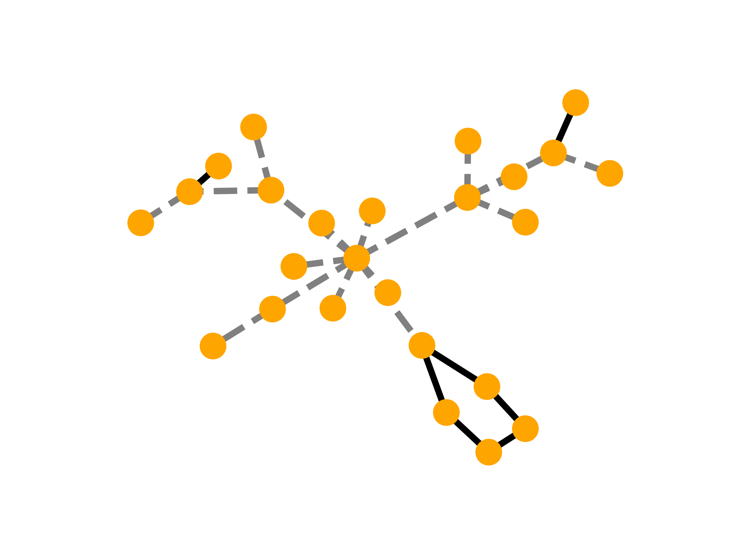
((c)) MixupExplainer

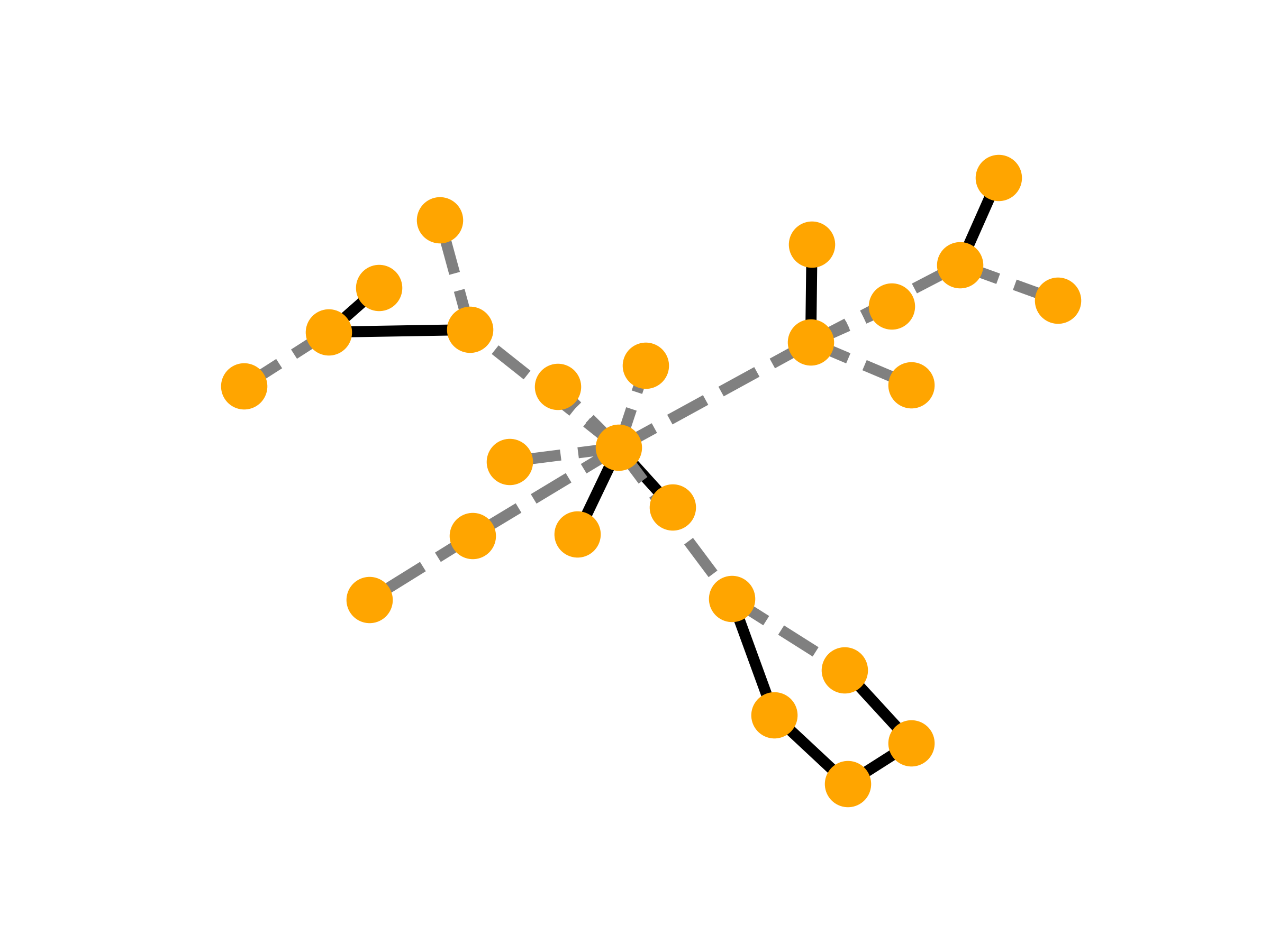
((d)) PGExplainer

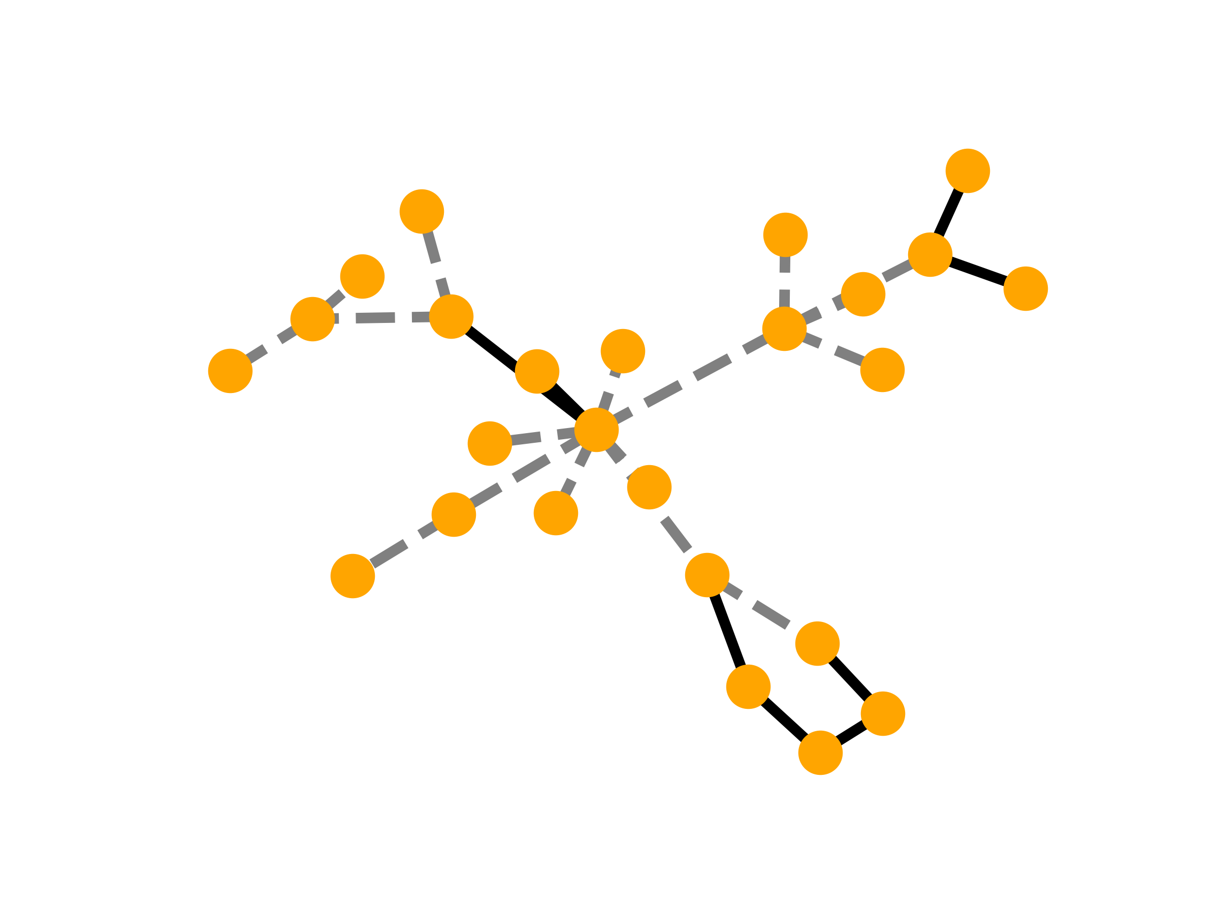
((e)) GNNExplainer

Figure 4: Visualization of explanation results from different explanation models on BA-2motifs. The generated explanations are highlighted by bold black edges.

((a)) Ground Truth

((b)) ProxyExplainer

((c)) MixupExplainer

((d)) PGExplainer

((e)) GNNExplainer

Figure 5: Visualization of explanation results from different explanation models on Benzene. The generated explanations are highlighted by bold orange edges.

The results demonstrate that ProxyExplainer provides the most accurate explanations across all datasets. Specifically, it improves the AUC scores by an average of $7.5\%$ on synthetic datasets and $12.3\%$ on real-world datasets. Comparisons with baseline methods highlight the advantages of our proposed explanation framework. Besides, ProxyExplainer captures underlying explanatory factors consistently across diverse datasets. For instance, MixupExplainer exhibits proficiency on the synthetic BA-2motifs dataset but performs poorly on the real-world Benzene dataset. The reason is that MixupExplainer relies on the independence assumption of explanation and non-explanation subgraphs, which may not hold in real-world datasets. In contrast, ProxyExplainer consistently demonstrates high performance across different datasets, showcasing its robustness and adaptability. We also replace the GCN with the Graph Isomorphism Network (GIN) in Appendix D.3 to demonstrate that ProxyExplainer can explain different GNN models.

Table 2: MMD results between the ground truth explanations and original graphs (GT); PGExplainer explanations and original graphs (PGE); proxy graphs in our methods and original graphs (Proxy).

Metric	BA-2motifs			BA-3motifs			Alkane-Carbonyl
	GT	PGE	Proxy	GT	PGE	Proxy	GT	PGE	Proxy
Deg.	0.846	0.785	0.032	0.646	0.209	0.135	0.663	0.525	0.225
Clus.	0.601	0.684	0.319	0.834	0.741	0.625	0.051	0.051	0.051
Spec.	0.278	0.289	0.023	0.259	0.108	0.103	0.635	0.469	0.049
Sum.	1.725	1.759	0.374	1.740	1.059	0.864	1.349	1.046	0.325
Metric	Benzene			Fluoride-Carbonyl			MUTAG
	GT	PGE	Proxy	GT	PGE	Proxy	GT	PGE	Proxy
Deg.	0.412	0.500	0.279	0.546	0.478	0.275	0.598	0.526	0.235
Clus.	0.059	0.001	0.052	0.049	0.049	0.049	0.029	0.029	0.071
Spec.	0.278	0.198	0.096	0.385	0.349	0.075	0.442	0.421	0.141
Sum.	0.749	0.698	0.427	0.980	0.876	0.399	1.070	0.976	0.448

6.3 Alleviating Distribution Shifts (RQ2)

In this section, we assess ProxyExplainer’s ability to generate in-distribution proxy graphs. Due to the intractable of direct computation, we follow the previous work (Chen et al., 2023) to compare distributions of multiple graph statistics, including degree distributions, clustering coefficients, and spectrum distributions, between the generated proxy graphs and original graphs. Specifically, we utilize Gaussian Earth Mover’s Distance kernel when computing MMDs. Smaller MMD values indicate similar graph distributions. For comparison, we also include the Ground truth explanations and the ones generated by PGExplainer.

The results are shown in Table 2. “GT” denotes the MMDs between the ground truth explanations and original graphs. “PGE” represents the MMDs between explanations generated by PGExplainer and original graphs. “Proxy” denotes the MMDs between proxy graphs in our method and original graphs. We have the following observations, first, the MMDs between Ground truth and original graphs are usually large, verifying our motivation that a model trained on original graphs may not have correct predictions on the OOD explanation subgraphs. Second, the explanations generated by a representative work, PGExplainer, are often OOD from original graphs, indicating that the original GIB-based objective function may be sub-optimal. Third, in most cases, proxy graphs generated by our method are with smaller MMDs, demonstrating their in-distribution property.

6.4 Ablation Studies (RQ3)

In this section, we conduct ablation studies to investigate the roles of different components. Specifically, we consider the following variants of ProxyExplainer: (1) w/o $G^{\Delta}$: in this variant, we remove the non-explanatory subgraph generator (VGAE), which is the bottom half as shown in Figure 2; (2) w/o $\mathcal{L}_{\text{KL}}$: in this variant, we remove the KL divergence from the training loss in ProxyExplainer; (3) w/o $\mathcal{L}_{\text{dist}}$: in this variant, we remove the distribution loss from ProxyExplainer. The results of the ablation study on BA-2motifs and Alkane-Carbonyl are reported in Figure 3.

Figure 3 illustrates a notable performance drop for all variants, indicating that each component contributes positively to the effectiveness of ProxyExplainer. Especially, in the real-life dataset, Alkane-Carbonyl, without the in-distribution constraint, w/o $\mathcal{L}_{\text{dist}}$ is much worse than ProxyExplainer, indicating the vital role of in-distributed proxy graphs in our framework. Extensive ablation studies on other datasets can be found in the Appendix D.2.

6.5 Case Studies

In this part, we conduct case studies to qualitatively compare the performances of ProxyExplainer against others. We adopt examples from BA-2motifs and Benzene in this part. We show visualization results in Figure 4 and Figure 5. Explanations are highlighted with bold black and bold orange edges, respectively. From the results, our ProxyExplainer stands out by generating more compelling explanations compared to baselines. Specifically, ProxyExplainer maintains clarity without introducing irrelevant edges and exhibits more concise results compared to alternative methods. The visualized performance underscores ProxyExplainer’s ability to provide meaningful and focused subgraph explanations. More visualizations on these two datasets can be found in the Appendix D.5.

7 Conclusion

In this paper, we systematically investigate the OOD problem in the de facto framework, GIB, for learning explanations in GNNs, which is highly overlooked in the literature. To address this issue, we extend the GIB by innovatively including in-distributed proxy graphs. On top of that, we derive a tractable objective function for practical implementations. We further present a new explanation framework that utilizes two graph auto-encoders to generate proxy graphs. We conduct comprehensive empirical studies on both benchmark synthetic datasets and real-life datasets to demonstrate the effectiveness of our method in alleviating the OOD problem and achieving high-quality explanations. There are several topics we will investigate in the future. First, the OOD problem also exists in obtaining model-level explanations and counterfactual explanations. We will extend our method to these research problems. Second, we will also analyze explainable learning methods with proxies in other data structures, such as image, language, and time series.

Impact Statements

This paper presents work whose goal is to advance the field of Machine Learning. There are many potential societal consequences of our work, none of which we feel must be specifically highlighted here.

Appendix A Notations

In Table 3, we summarized the main notations we used and their descriptions in this paper.

Table 3: Symbols and their descriptions.

Symbols	Descriptions
$\mathcal{G}$	A set of graphs
$G,{\mathcal{V}},{\mathcal{E}}$	Graph instance, node set, edge set
$v_{i}$	The $i$-th node
${\bm{X}}$	Node feature matrix
${\bm{A}}$	Adjacency matrix
${\bm{Z}}$	Node representation matrix
$Y$	Label of graph $G$
$\mathcal{C}$	A set of labels
$G^{*}$	Optimal explanatory subgraph
${\mathcal{G}}^{*}$	A set of $G^{*}$
$G^{\prime}$	Candidate explanatory subgraph
$G^{\Delta}$	Non-explanatory graph
$\tilde{G}$	Proxy graph of $G^{\prime}$ with a fixed distribution
h, $\textit{{h}}^{\prime}$, $\tilde{\textit{{h}}}$	Graph embedding
$d$	Dimension of node feature
$D$	Dimension of node latent embedding
$f(\cdot)$	To-be-explained GNN model
$\Psi_{\psi}$	Explanation function
$\psi$	Parameter of the explanation function
$t_{\psi}(\cdot)$	Perturbation function
$P_{\mathcal{G}}$	Distribution of original training graphs
$P_{{\mathcal{G}}^{\prime}}$	Distribution of explanation subgraphs
$Q_{\bm{\phi}}$	Parameterized function of $P(\tilde{G}|G^{\prime})$
$\bm{\phi}$	Model parameters of $Q_{\bm{\phi}}$
$\bm{\phi}^{*}$	Optimal $\bm{\phi}$
$\alpha$	Balance parameter between $I(G,G^{\prime})$ and $I(Y,G^{\prime})$
$\bar{{\mathcal{E}}}$	The set of node pairs that are unconnected in $G$
$\tilde{p}_{uv}$	Probability of node pair $(u,v)$ in $\tilde{G}$
$\beta$	A hyper-parameter to get a trade-off between connected and unconnected node pairs
$f_{\text{enc}}(\cdot)$	The front part of GNNs that learns node representations
$f_{\text{cls}}(\cdot)$	The back part of GNNs that predicts graph labels based on node embeddings
$\sigma(\cdot)$	Sigmoid function
$\tau$	Temperature hyper-parameter for approximation
$\lambda$	A hyper-parameter in Proxy loss function
$\mathcal{L}_{\text{dist}}$	Distribution loss between $\tilde{G}$ and $G$
$\mathcal{L}_{\text{KL}}$	KL divergence between distribution of ${\bm{Z}}^{\Delta}$ and its prior
$\mathcal{L}_{\text{proxy}}$	Proxy loss
$\mathcal{L}_{\text{exp}}$	Explainer loss

Appendix B Algorithm

We take as input a set of graphs $\mathcal{G}=\{G_{i}\}_{i=0}^{N}$. For each graph $G_{i}$, we use an explainer model to identify a subgraph $G^{\prime}_{i}$ as the explanation and then compute the non-explanatory graph $G^{\Delta}_{i}$, which is obtained by removing edges in $G_{i}$ that exist in $G^{\prime}_{i}$. We use GAE to reconstruct a subgraph, denoted by $\tilde{G}^{\prime}_{i}$ from the subgraph $G’_{i}$ and another VGAE to generate a new subgraph, denoted by $\tilde{G}^{\Delta}_{i}$, from the non-explainable subgraph $G^{\Delta}_{i}$. The proxy graph, $\tilde{G}_{i}$, is obtained by combining them, whose adjacency matrix can be denoted by $\tilde{{\bm{A}}}_{i}=\tilde{{\bm{A}}}^{\prime}_{i}+\tilde{{\bm{A}}}^{\Delta}_{i}$. Here $\tilde{{\bm{A}}}^{\prime}_{i}$ and $\tilde{{\bm{A}}}^{\Delta}_{i}$ are adjacency matrices of $\tilde{G}^{\prime}_{i}$ and $\tilde{G}^{\Delta}_{i}$, respectively. We alternatively train the explainer model and proxy graph generator as shown in Algorithm 1.

Algorithm 1 Algorithm of ProxyExplainer

  Input: A set of graphs $\mathcal{G}=\{G_{i}\}_{i=0}^{N}$, with each $G_{i}=({\mathcal{V}}_{i},{\mathcal{E}}_{i},{\bm{X}}_{i}),$a pretrain to-be-explained model $f(\cdot)$, hyper parameters $\alpha,\lambda,M$, epochs $E$.

  Initialize an explainer function $\Psi_{\psi}(\cdot)$

  $\text{epoch}\leftarrow 0$

  while epoch $<E$ do

     for $G_{i}\in\mathcal{{\bm{G}}}$ do

        $G^{\prime}_{i}\leftarrow\Psi_{\psi}(G_{i})$

        $G^{\Delta}_{i}\leftarrow$ $G_{i}-G^{\prime}_{i}$

        Compute $\tilde{{\bm{A}}}^{\prime}_{i}$ with equation 14

        Compute ${\bm{Z}}^{\Delta}$ and $\tilde{{\bm{A}}}^{\Delta}_{i}$ with equation 16

        compute proxy loss $\mathcal{L}_{\text{proxy}}$ with equation 18

        Update parameters in proxy graph generator with backpropagation

        if  epoch$\%M==0$ then

           compute explainer loss $\mathcal{L}_{\text{exp}}$

           Update parameters in the explainer with backpropagation.

        end if

     end for

     $\text{epoch}\leftarrow\text{epoch}+1$

  end while

Appendix C Full Experimental Setups

C.1 Datasets

BA-2motifs (Luo et al., 2020). The BA-2motifs dataset consists 1,000 synthetic graphs, each derived from a basic Barabasi-Albert (BA) model. The dataset is divided into two categories: one part of the graphs add patterns that mimic the structure of a house, and the remaining integrate five-node cyclic patterns. The classification of these graphs depends on the specific patterns.
BA-3motifs (Chen et al., 2023). BA-3motifs is an extended dataset inspired by the BA-2motifs and contains 3,000 synthetic graphs. Each base graph is accompanied by one of three different patterns: house, cycle, or grid.
Alkane-Carbonyl (Sánchez-Lengeling et al., 2020). The Alkane-Carbonyl dataset consists of a total of 4,326 molecule graphs that are categorized into two different classes. Positive samples refer to molecules that have both alkane and carbonyl functional groups. The ground-truth explanation includes alkane and carbonyl functional groups in a given molecule.
Benzene (Sánchez-Lengeling et al., 2020). Benzene consists 12,000 molecular graphs from the ZINC15(Sterling & Irwin, 2015) database, which can be classified into two classes. The main goal is to determine if a Benzene ring is exited in each molecule. In cases where multiple Benzene rings are present, each Benzene ring is treated as a distinct explanation.
Fluoride-Carbonyl (Sánchez-Lengeling et al., 2020). The Fluoride-Carbonyl dataset has 8,671 molecular graphs. The ground-truth explanation is based on the particular combination of fluoride atoms and carbonyl functional groups present in each molecule.
MUTAG (Kazius et al., 2005). MUTAG dataset includes 4,337 molecular graphs, each of them is classified into two groups based on its mutagenic effect on the Gram-negative bacterium S. Typhimurium. This classification comes from several specific virulence gland groups with mutagenicity in molecular mapping by Kazius et al.(Kazius et al., 2005).

Table 4: Statistics of molecule datasets for graph classifcation with ground-truth explanations.

	BA-2motifs	BA-3motifs	Alkane-Carbonyl	Benzene	Fluoride-Carbonyl	MUTAG
Graphs	1,000	3,000	4,326	12,000	8,671	4,337
Average nodes	25.00	21.92	21.13	20.58	21.36	29.15
Average edges	25.48	29.51	44.95	43.65	45.37	60.83
Original graph
Features	None	None	Atom	Atom	Atom	Atom
Ground truth explanation
	House, cycle	House,cycle, grid	Alkane,C=O	Benzene Ring	F-,C=O	NH2, NO2

Table 5: The graph-classification task performances of the GCN model

	BA-2motifs	BA-3motifs	Alkane-Carbonyl	Benzene	Fluoride-Carbonyl	MUTAG
Train Acc	0.999	0.997	0.979	0.930	0.951	0.850
Val Acc	1.0	0.997	0.986	0.923	0.956	0.834
Test Acc	1.0	0.977	0.975	0.915	0.951	0.804

C.2 Baselines

To evaluate our model, we well-train the GCN model in to ensure that it takes good performance in graph classification tasks. The results are displayed in Table 5. We utilize a well-established explanation method as a benchmark baseline PGExplainer. Furthermore, for a comprehensive comparison, we incorporate various post-hoc explanation methods, including GradCAM, GNNExplainer, PGExplainer, ReFine, and MixupExplainer.

• GradCAM (Pope et al., 2019). This method utilizes gradients as a weighting mechanism to merge various feature maps. It operates on heuristic assumptions and cannot elucidate node classification models.

• GNNExplainer (Ying et al., 2019). It learns soft masks for edges and node features, and aims to elucidate predictions through mask optimization. GNNExplainer integrates these masks with the original graph through element-wise multiplications. The masks are optimized by enhancing the mutual information between the original graph and the modified graph prediction results.

• PGExplainer (Luo et al., 2020). This method extends the idea of GNNExplainer by assuming that the graph is a random Gilbert graph. PGExplainer generates each edge embedding by combining the embeddings of its constituent nodes, then uses these edge embeddings to determine a Bernoulli distribution to indicate whether to mask an edge or not, and utilizes a Gumbel-Softmax approach to model the Bernoulli distribution for end-to-end training.

• ReFine (Wang et al., 2021). ReFine identifies the edge probabilities for the entire category by maximizing the mutual information and contrastive loss between categories. In fine-tuning, it uses the edge probabilities from the previous stage to sample edges, and find explanations that maximize mutual information for specific instances.

• MixupExplainer (Zhang et al., 2023b). This method combines original explanatory subgraphs with randomly sampled, label-independent base graphs in a non-parametric way to mitigate the common OOD issue which found in previous methods.

Appendix D Extensive Experiments

D.1 Extensive Distribution Analysis

As shown in previous work (Zhang et al., 2023b), another way to approximate the distribution differences of graphs is to compare their vector embeddings. Here, we adopt the same setting and use Cosine similarity and Euclidean distance to intuitively approximate the similarities between graph distributions. Table 6 presents the computed Cosine similarity and Euclidean distance between the distribution embeddings of the original graph h, the ground truth explanation subgraph $\textit{{h}}^{\prime}$, and the generated proxy graph $\tilde{\textit{{h}}}$. Notably, our proxy graph embedding $\tilde{\textit{{h}}}$ exhibits higher Cosine similarity scores and lower Euclidean distance with the original graph embedding h compared to the ground truth explanation embedding $\textit{{h}}^{\prime}$. We observe an average improvement of $17.9\%$ in Cosine similarity and $33.6\%$ in Euclidean distance. Particularly in the BA-2motifs dataset, there is a significant improvement of $60.4\%$ in Cosine similarity and $51.8\%$ in Euclidean distance. These findings underscore the effectiveness of our ProxyExplainer method in mitigating distribution shifts caused by induction bias in the to-be-explained GNN model $f(\cdot)$, thereby enhancing explanation performance.

Table 6: The Cosine score and Euclidean distance between the distribution embedding of the original graph h, explanation subgraph $\textit{{h}}^{\prime}$, and our proxy graph $\tilde{\textit{{h}}}$ on different datasets.

	BA-2motifs	BA-3motifs	Alkane-Carbonyl	Benzene	Fluoride-Carbonyl	MUTAG
Avg. Cosine(h, $\textit{{h}}^{\prime}$) $\uparrow$	0.571	0.686	0.879	0.859	0.906	0.883
Avg. Cosine(h, $\tilde{\textit{{h}}}$) $\uparrow$	0.916	0.918	0.938	0.905	0.908	0.985
Avg. Euclidean(h, $\textit{{h}}^{\prime}$) $\downarrow$	1.210	1.199	0.912	0.893	0.805	0.975
Avg. Euclidean(h, $\tilde{\textit{{h}}}$) $\downarrow$	0.583	0.613	0.719	0.767	0.779	0.368

D.2 Extensive Ablation Study

In Figure 6, we conduct a comprehensive ablation study across all datasets to examine the impact of different components. The findings illustrate the effectiveness of these components and their positive contribution to our ProxyExplainer.

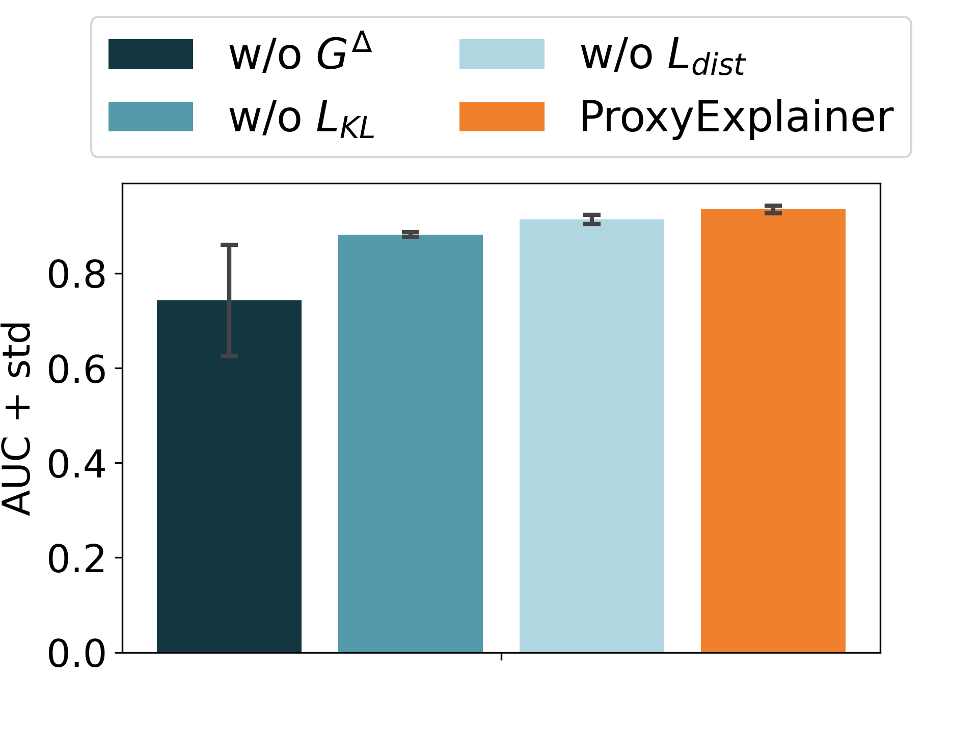
((a)) BA-2motifs

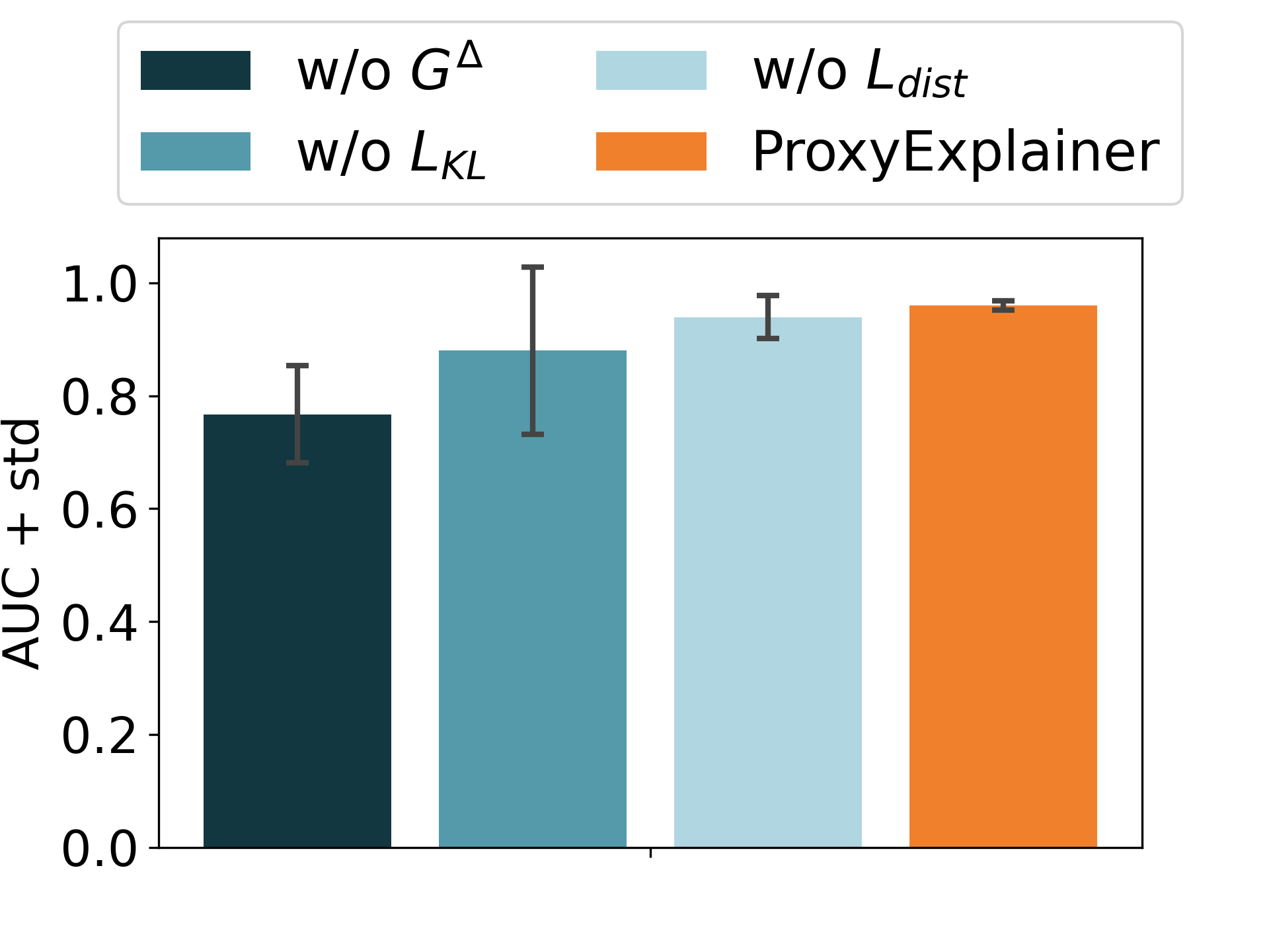
((b)) BA-3motifs

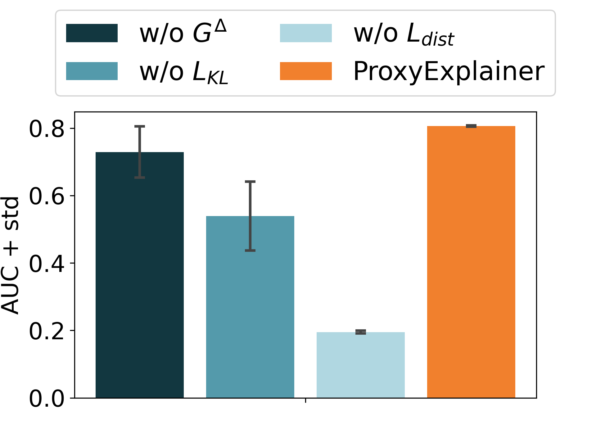
((c)) Alkane-Carbonyl

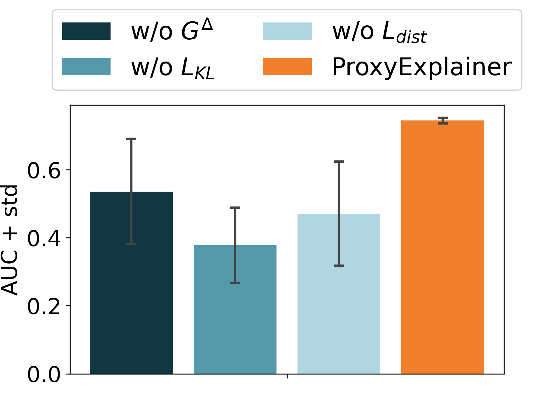
((d)) Benzene

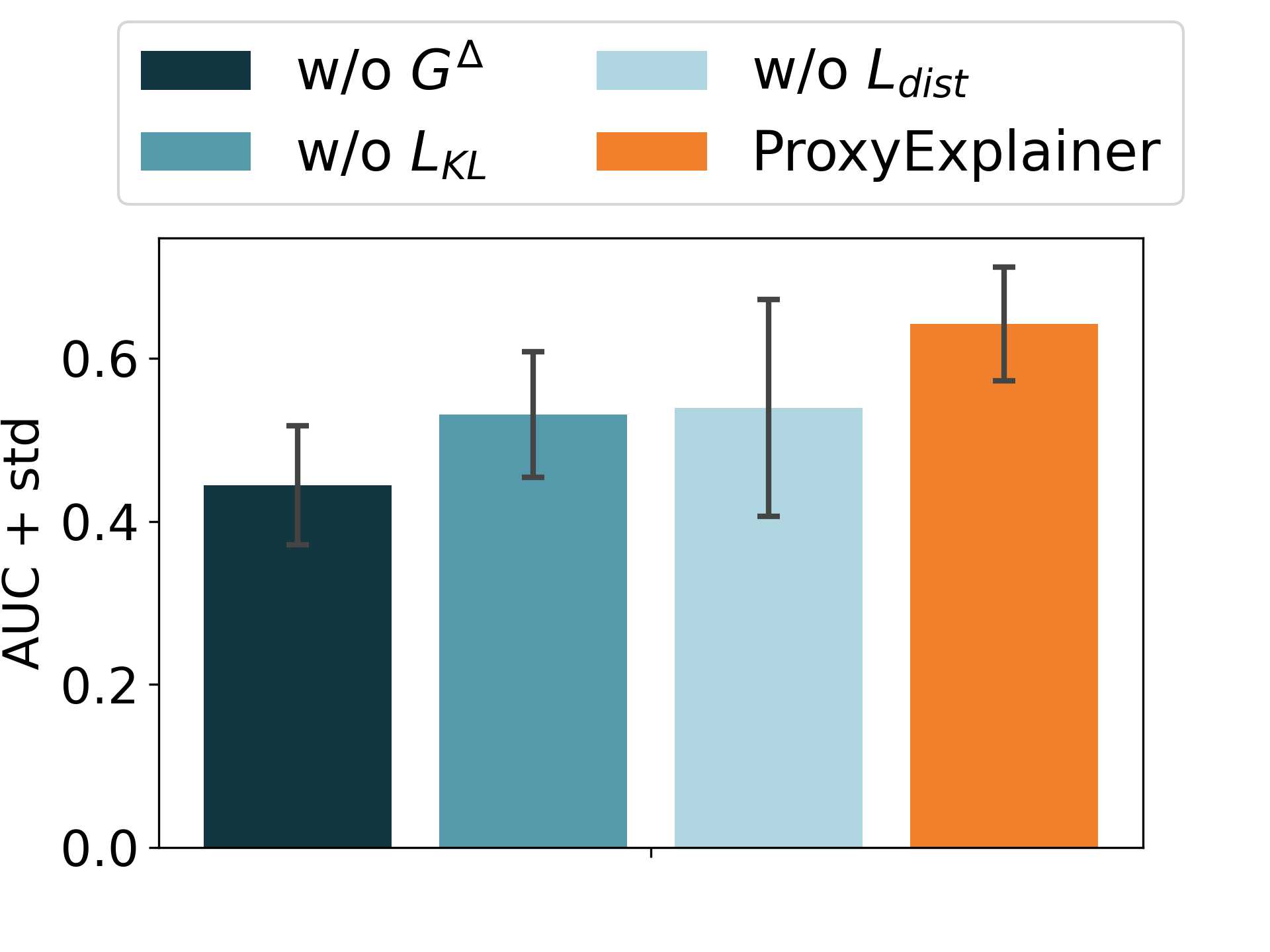
((e)) Fluoride-Carbonyl

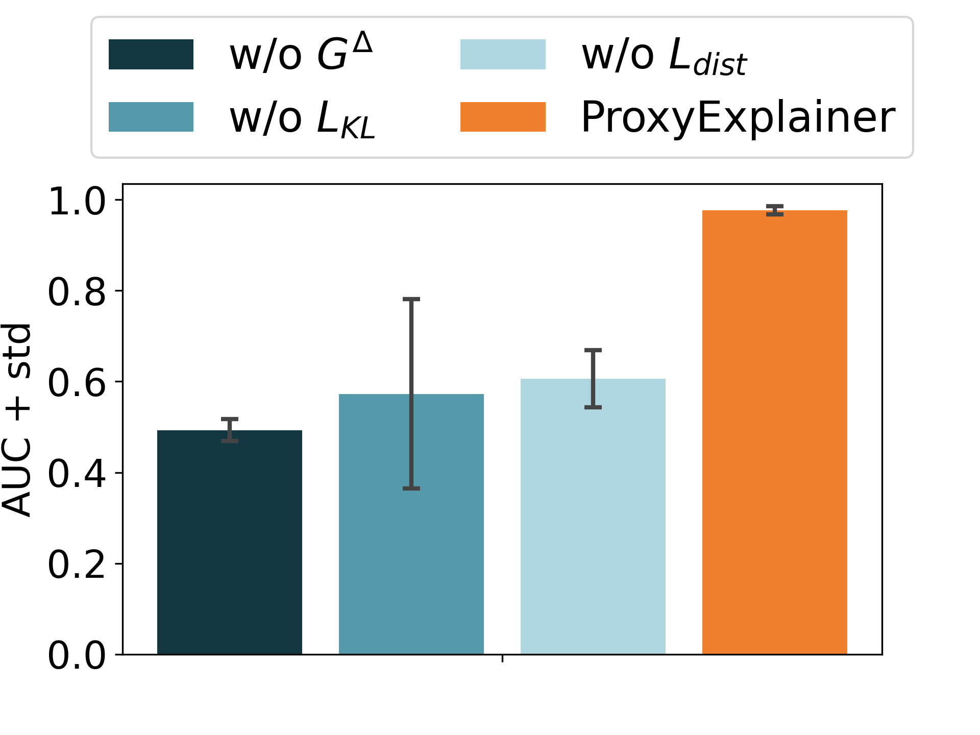
((f)) MUTAG

Figure 6: Ablation study on all datasets.

D.3 Extensive experiment with GIN

In order to show the robustness of our ProxyExplainer in explaining different GNN models, we first pre-train GIN on two synthetic datasets and two real-world datasets to ensure that GIN has the ability to classify graphs accurately. The results are displayed in Figure 7. Then we use both baseline methods in the previous experiment and our method ProxyExplainer to provide explanations for the pre-trained GIN model. As seen in Figure 8, it is noticeable that ProxyExplainer achieves the best performance on these datasets. Specifically, it improves the AUC scores of $45.9\%$ on BA-2motifs, $6.1\%$ on BA-3motifs, $2.4\%$ on Alkane-Carbonyl, and $12.5\%$ on Fluoride-Carbonyl. From the analysis, we can see that our ProxyExplainer can identify accurate explanations across different datasets.

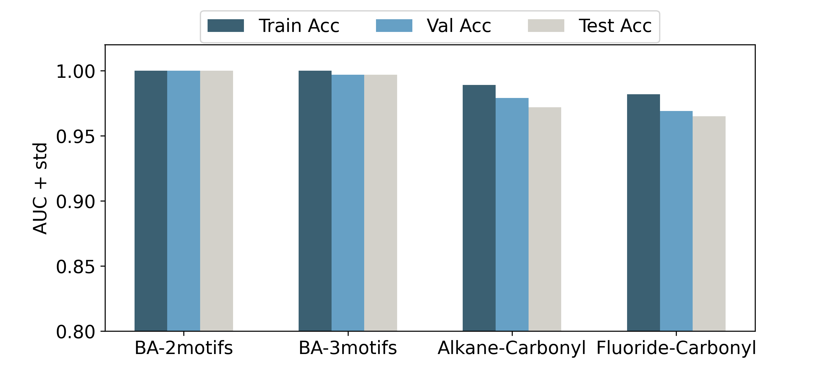
Figure 7: The graph-classification task performances of the GIN model.

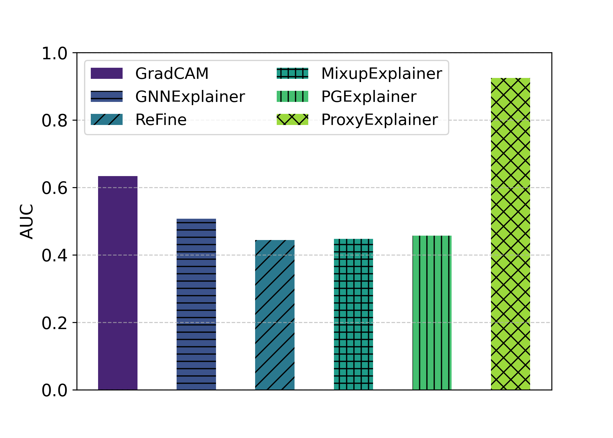
((a)) BA-2motifs

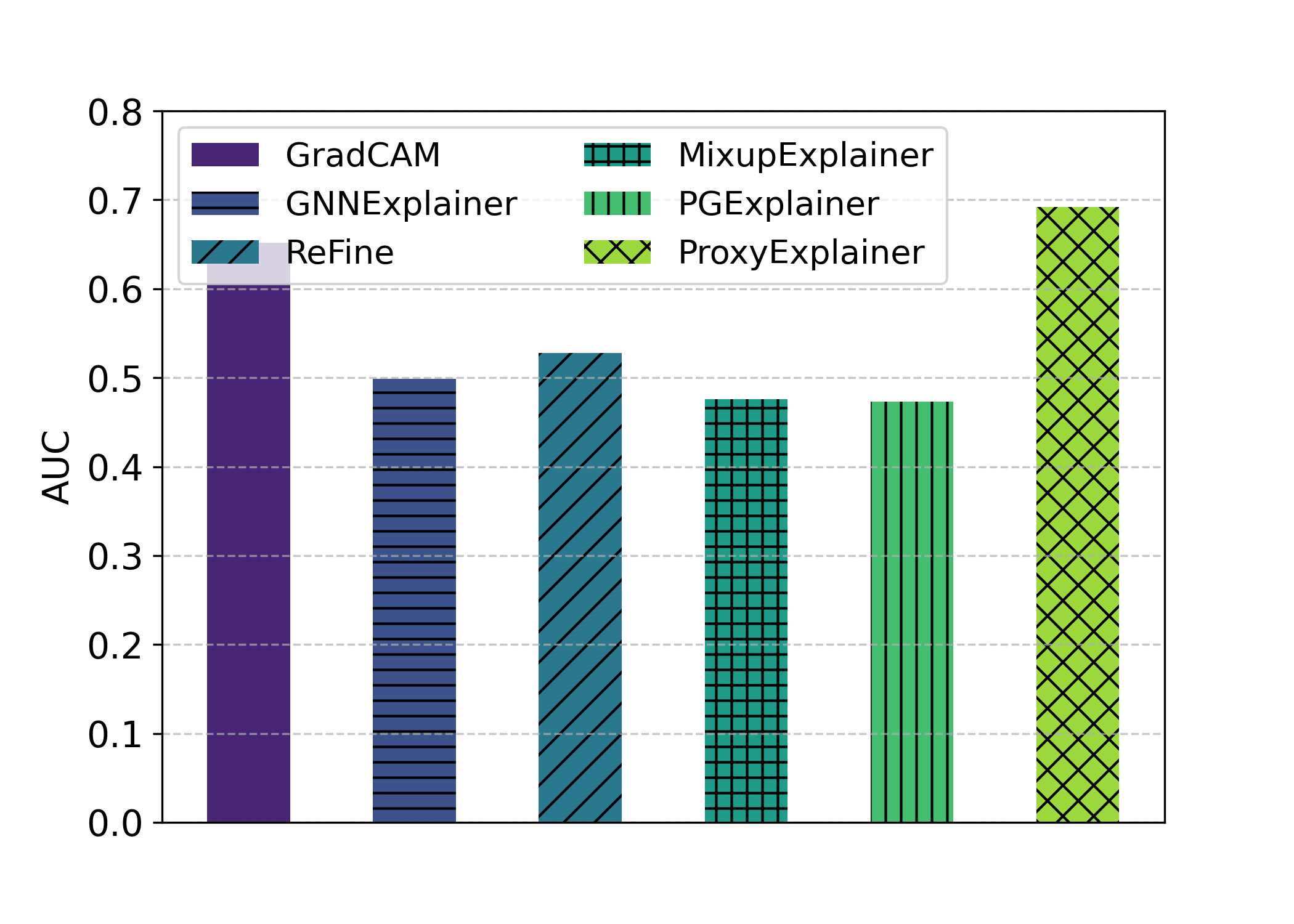
((b)) BA-3motifs

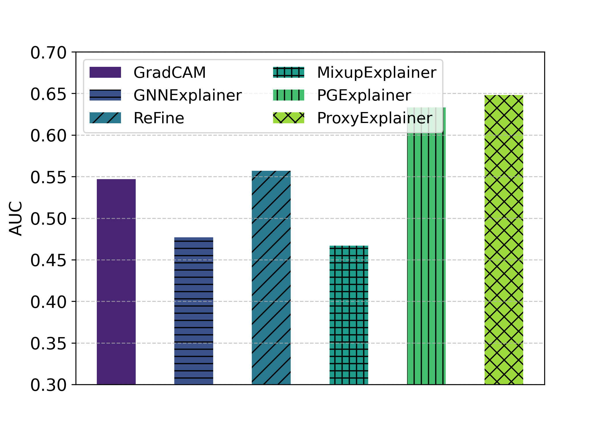
((c)) Alkane-Carbonyl

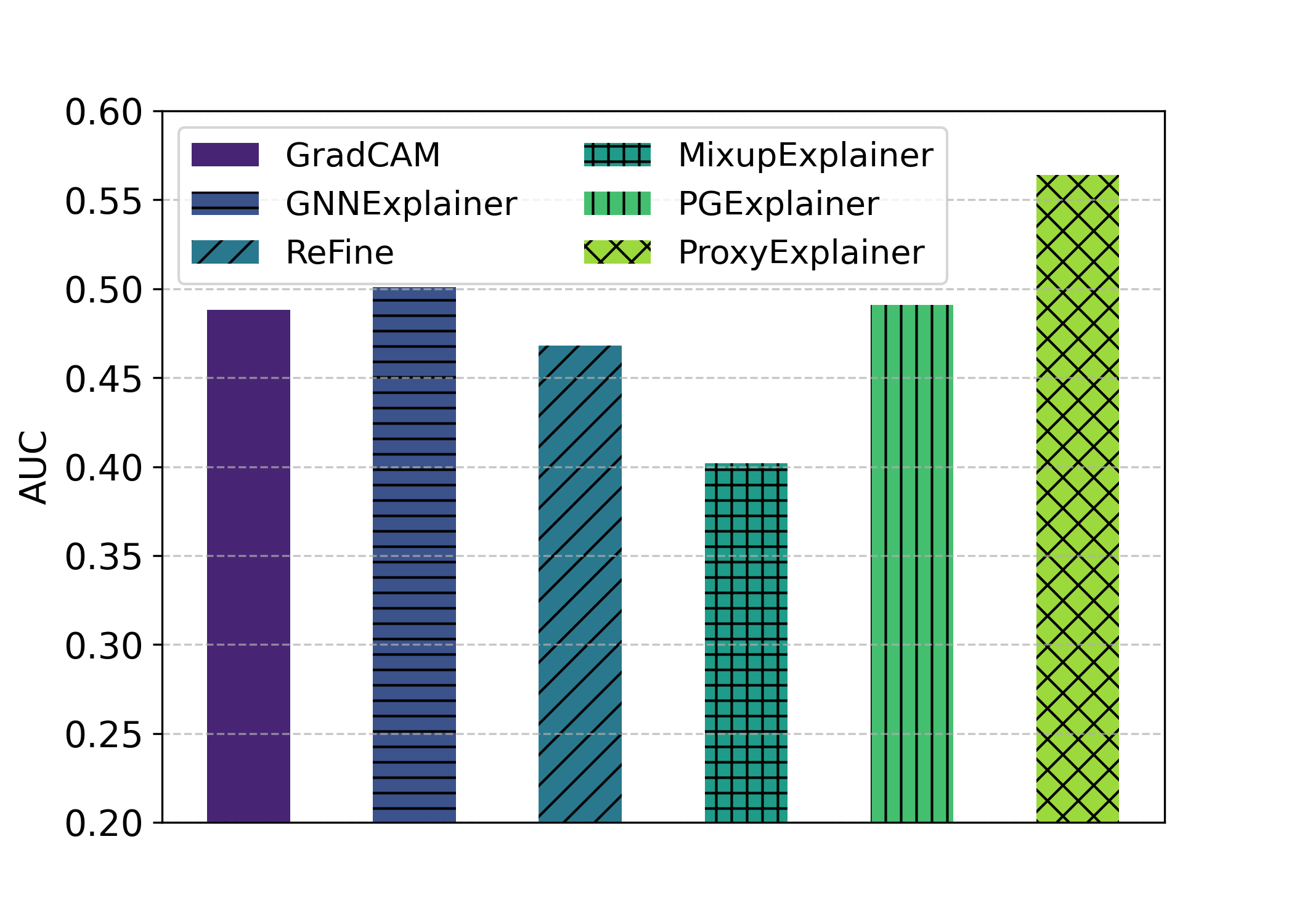
((d)) Fluoride-Carbonyl

Figure 8: Explanation accuracy in terms of AUC-ROC on edges based on GIN.

D.4 Parameter Sensitive Analysis

In this section, we analyze the influence of parameters including $\lambda$, which controls the KL divergence during the proxy graph generation process, and the dimension $D$ of node latent embedding. We vary $\lambda$ from 0.01 to 1.0. For $D$, we vary it among {32, 64, 128, 256, 512, 1024}. We only change the value of a specific parameter while fixing the remaining parameters to their respective optimal values.

Figure 9 shows the performance of our ProxyExplainer with respect to $\lambda$ on two synthetic datasets (BA-2motifs and BA-3motifs) and two real-world datasets (Alkane-Carbonyl and MUTAG). From Figure 9, we can see that ProxyExplainer consistently outperforms the best baseline, MixupExplainer, for $\lambda\in[0.25,1.0]$. This indicates that ProxyExplainer is stable. Figure 10 presents how the dimension of node latent embedding affects performance in ProxyExplainer, the results show that ProxyExplainer can reach the best performance at $D=512$.

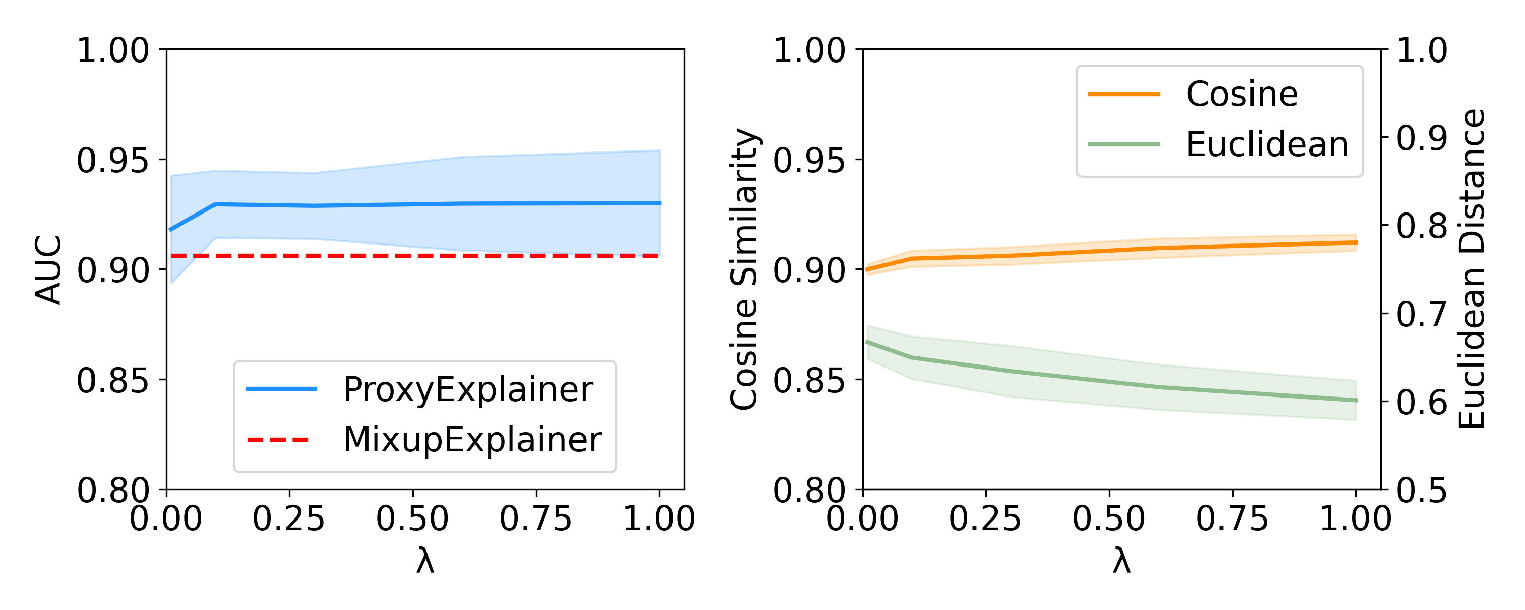
((a)) BA-2motifs

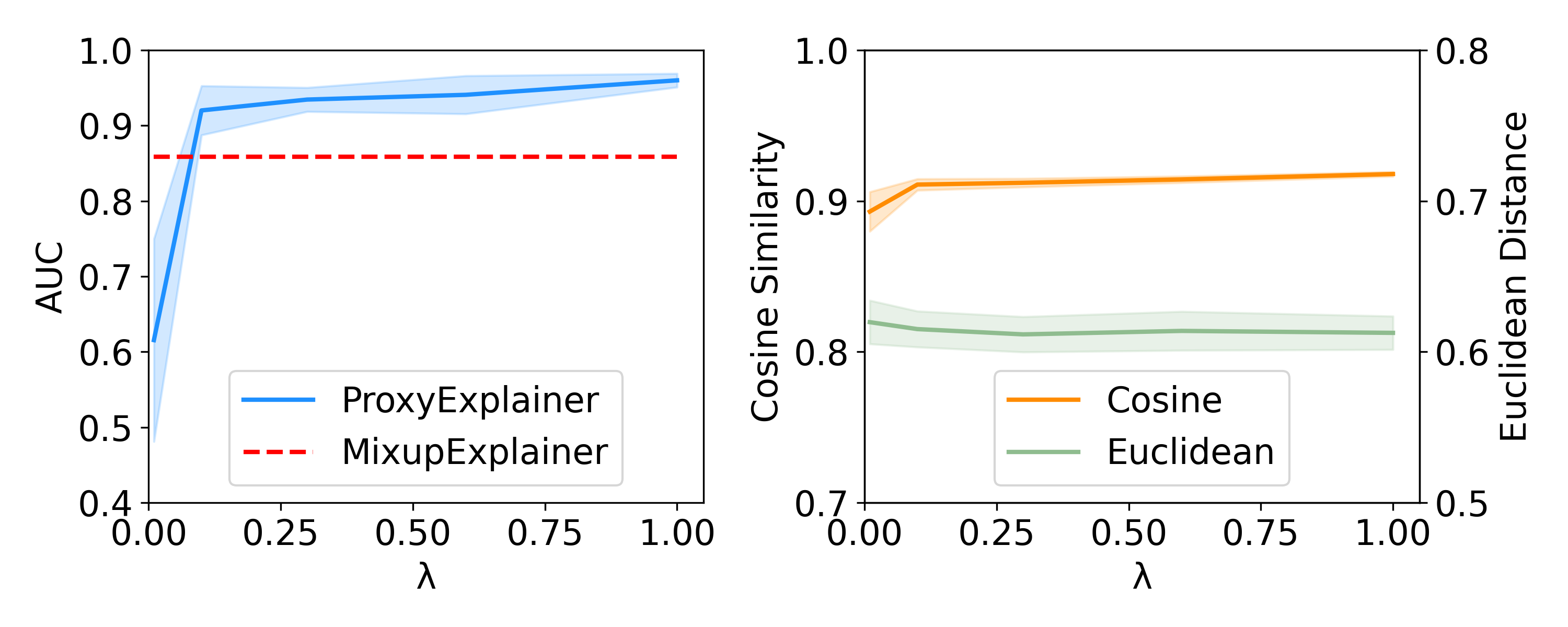
((b)) BA-3motifs

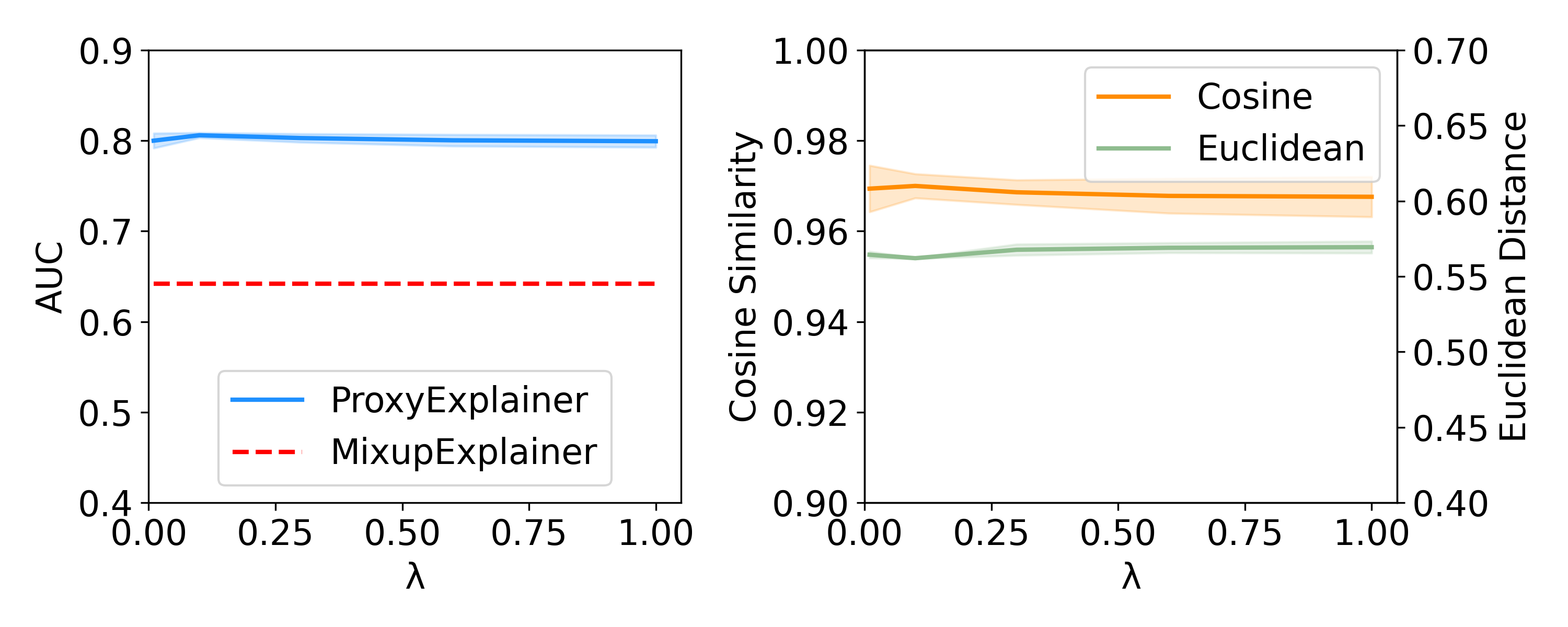
((c)) Alkane-Carbonyl

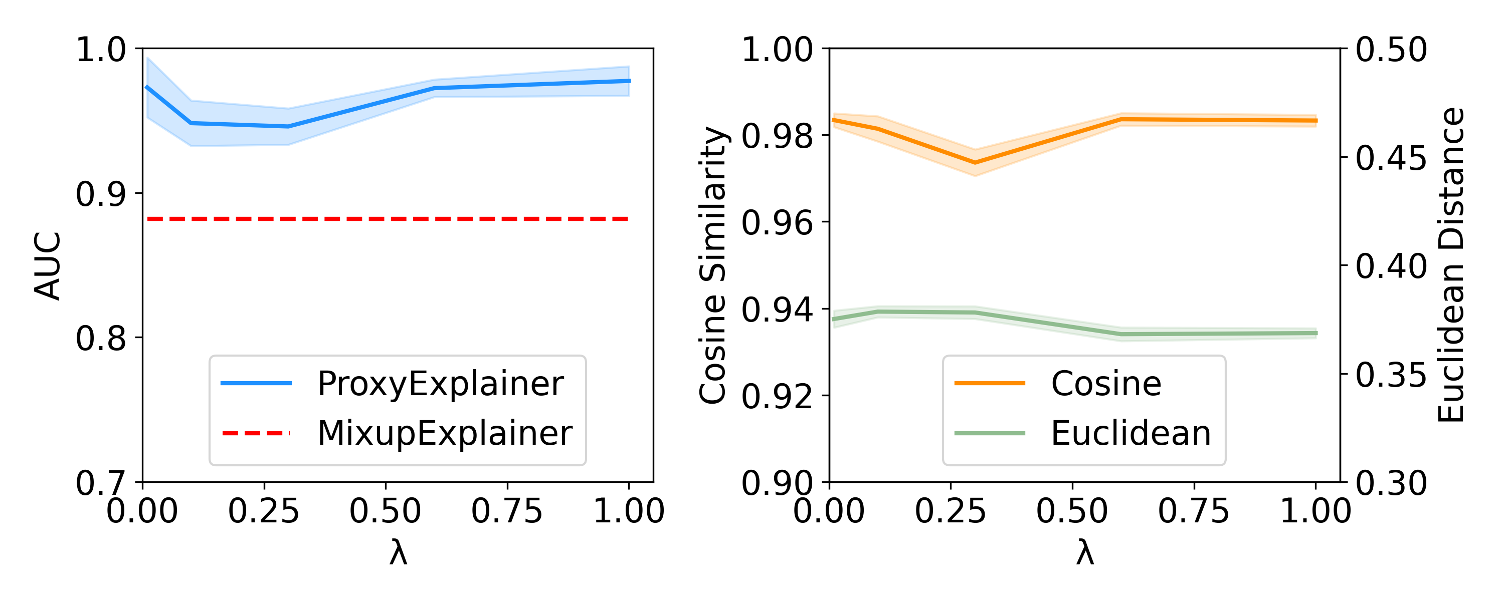
((d)) MUTAG

Figure 9: Parameter analysis of $\lambda$ on four datasets. The left side of each graph shows the explanation performance. The right side shows the Distance Analysis between h and $\tilde{\textit{{h}}}$.

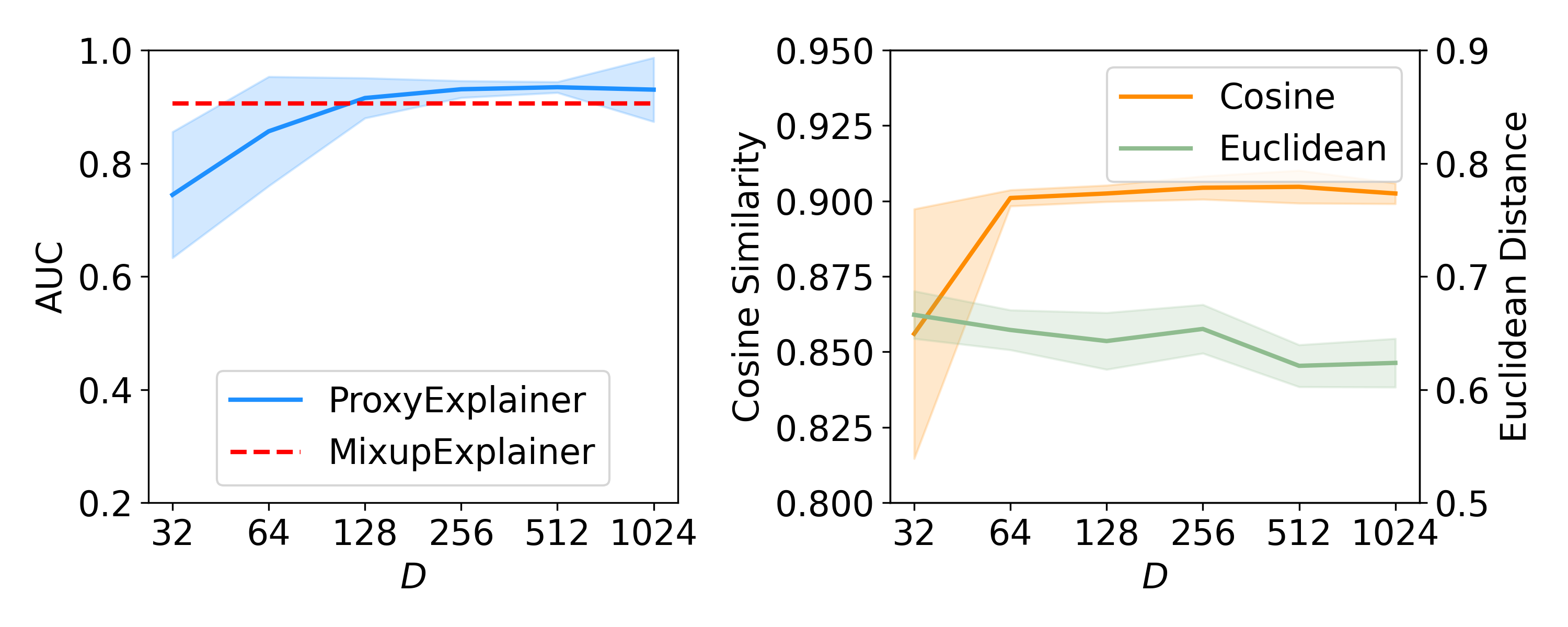
((a)) BA-2motifs

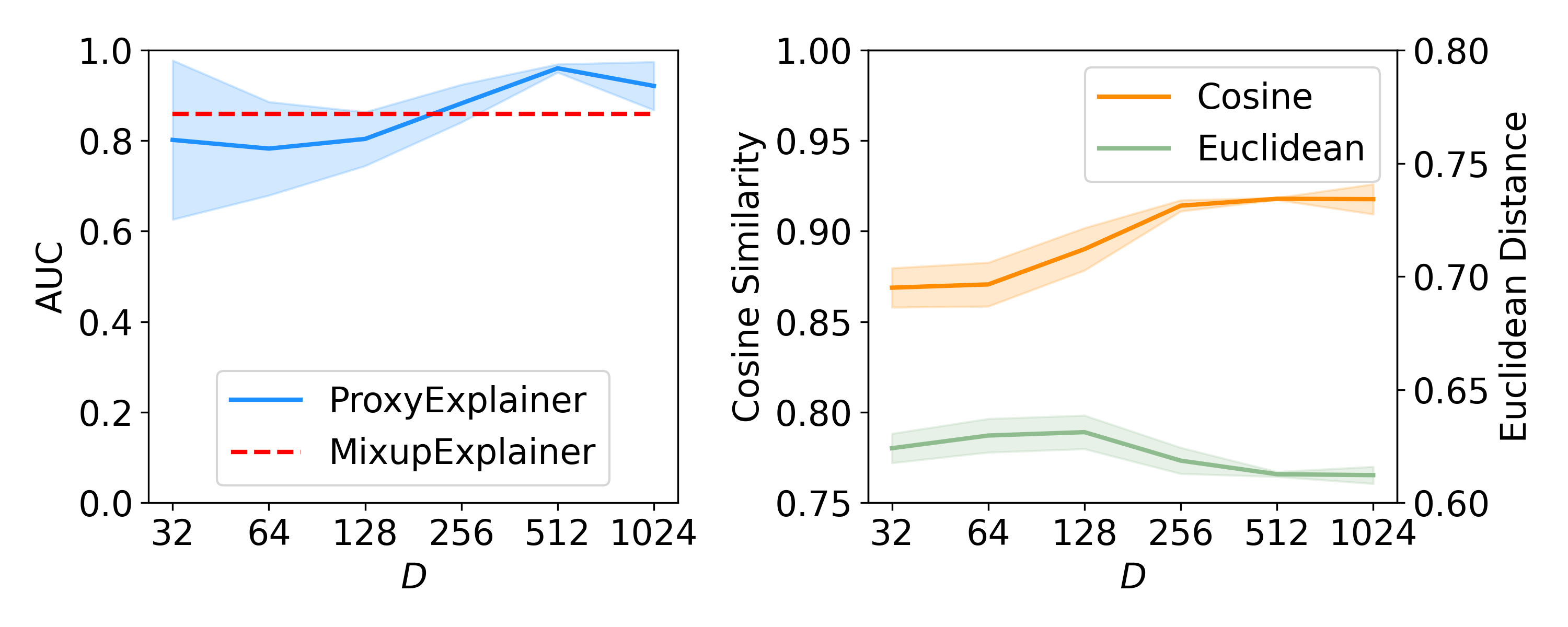
((b)) BA-3motifs

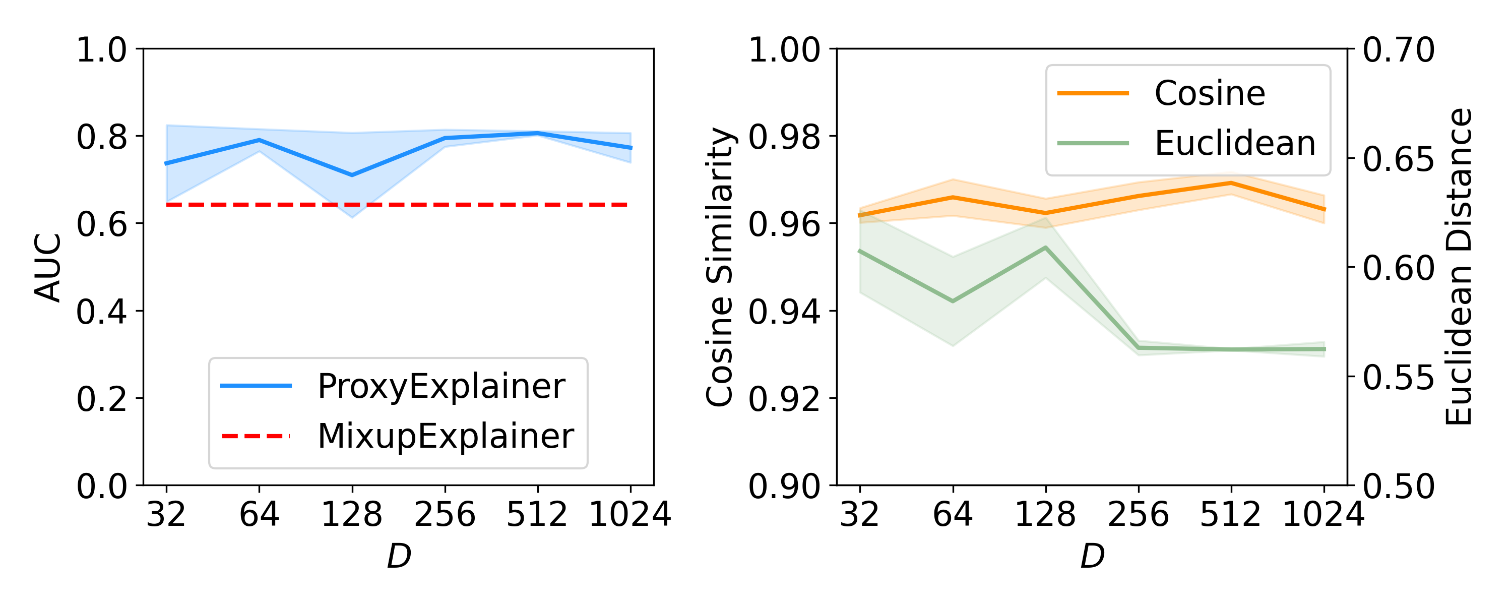
((c)) Alkane-Carbonyl

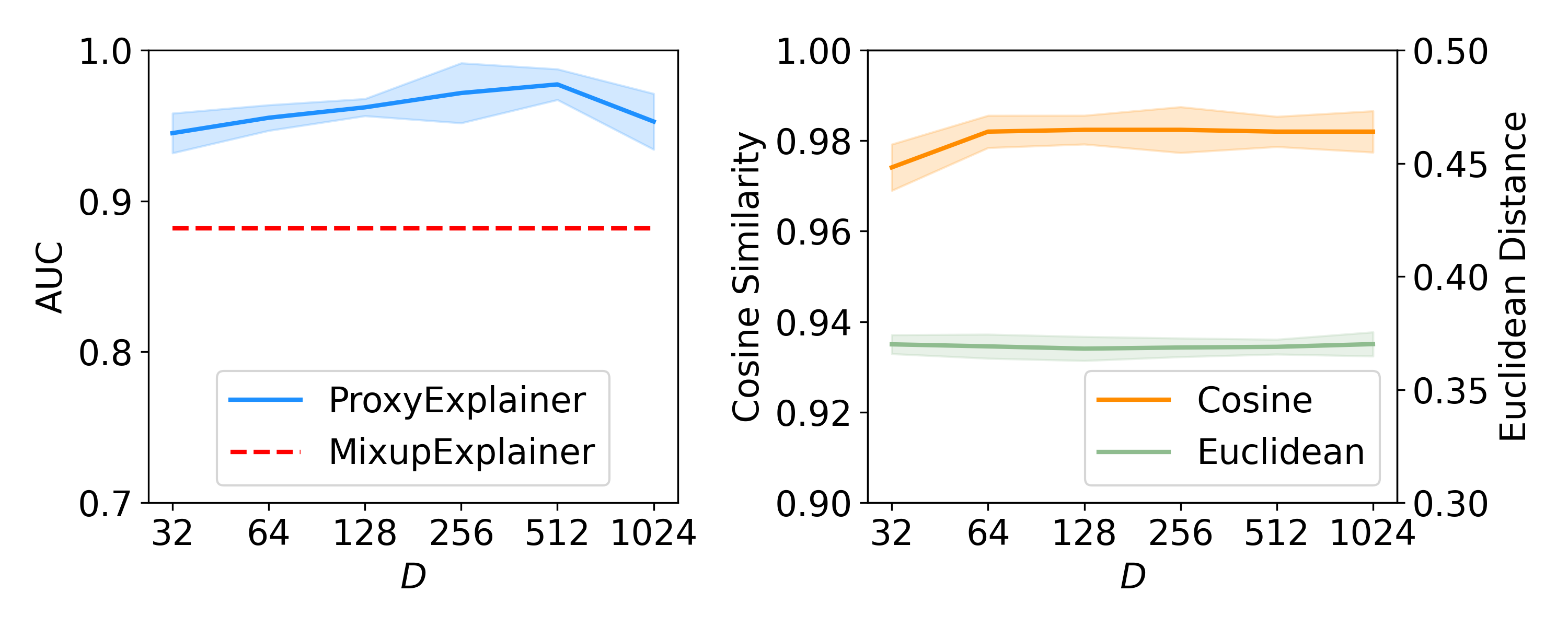
((d)) MUTAG

Figure 10: Parameter analysis of the dimension of node latent embedding. The left side of each graph shows the explanation performance and the right side displays the Cosine score and Euclidean distance between h and $\tilde{\textit{{h}}}$.

D.5 Extensive Case Study

We show more visualization examples of explanation graphs on BA-2motifs, BA-3motifs and Benzene in Figure 11, Figure 12, and Figure 13, respectively.

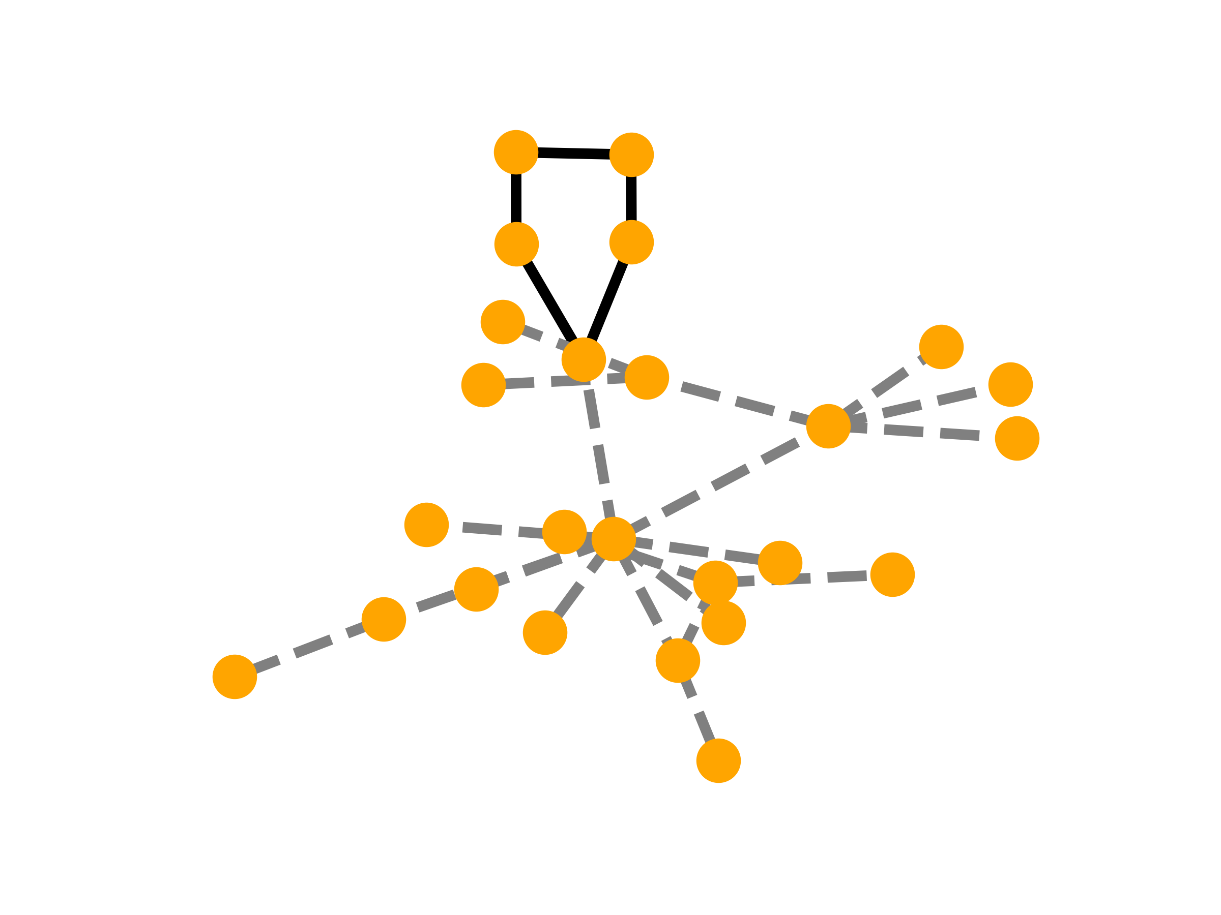
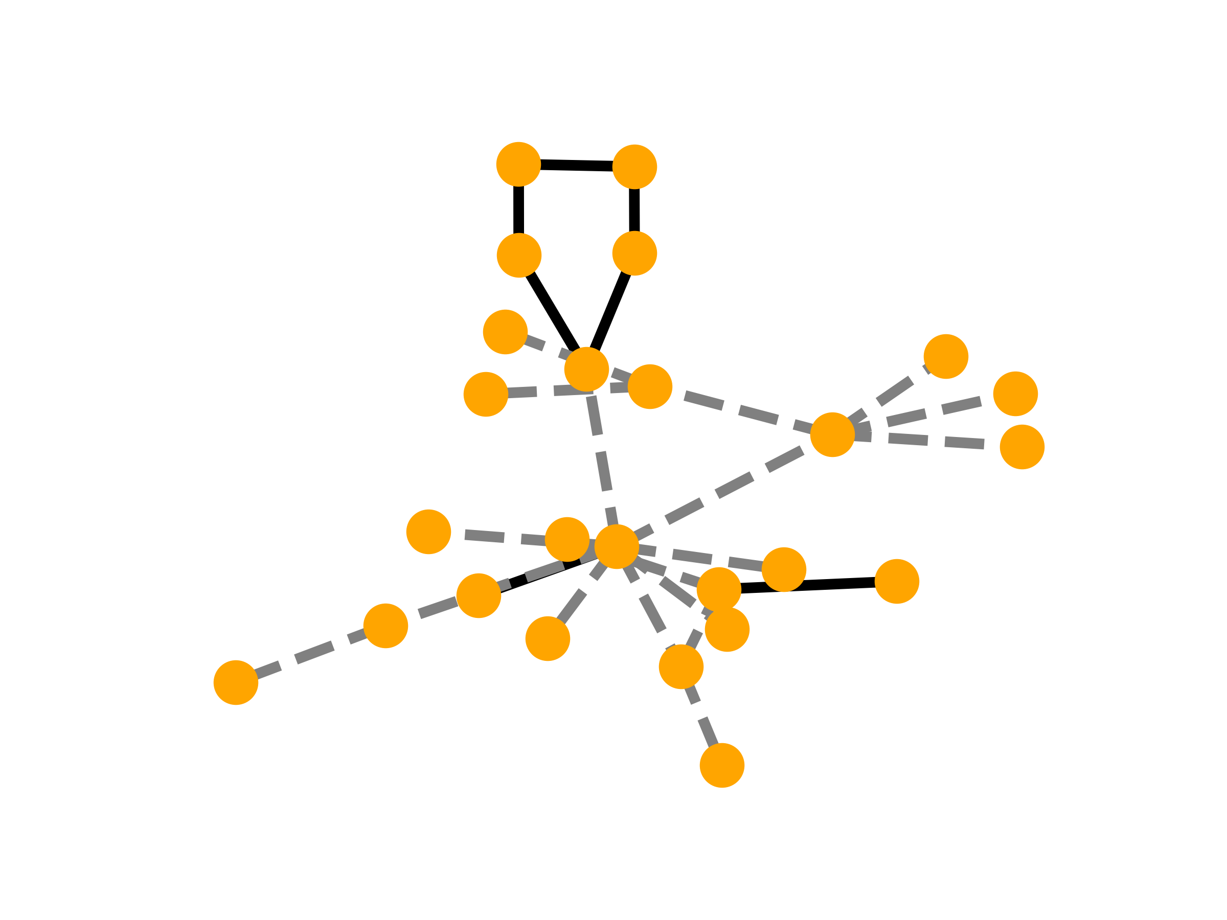
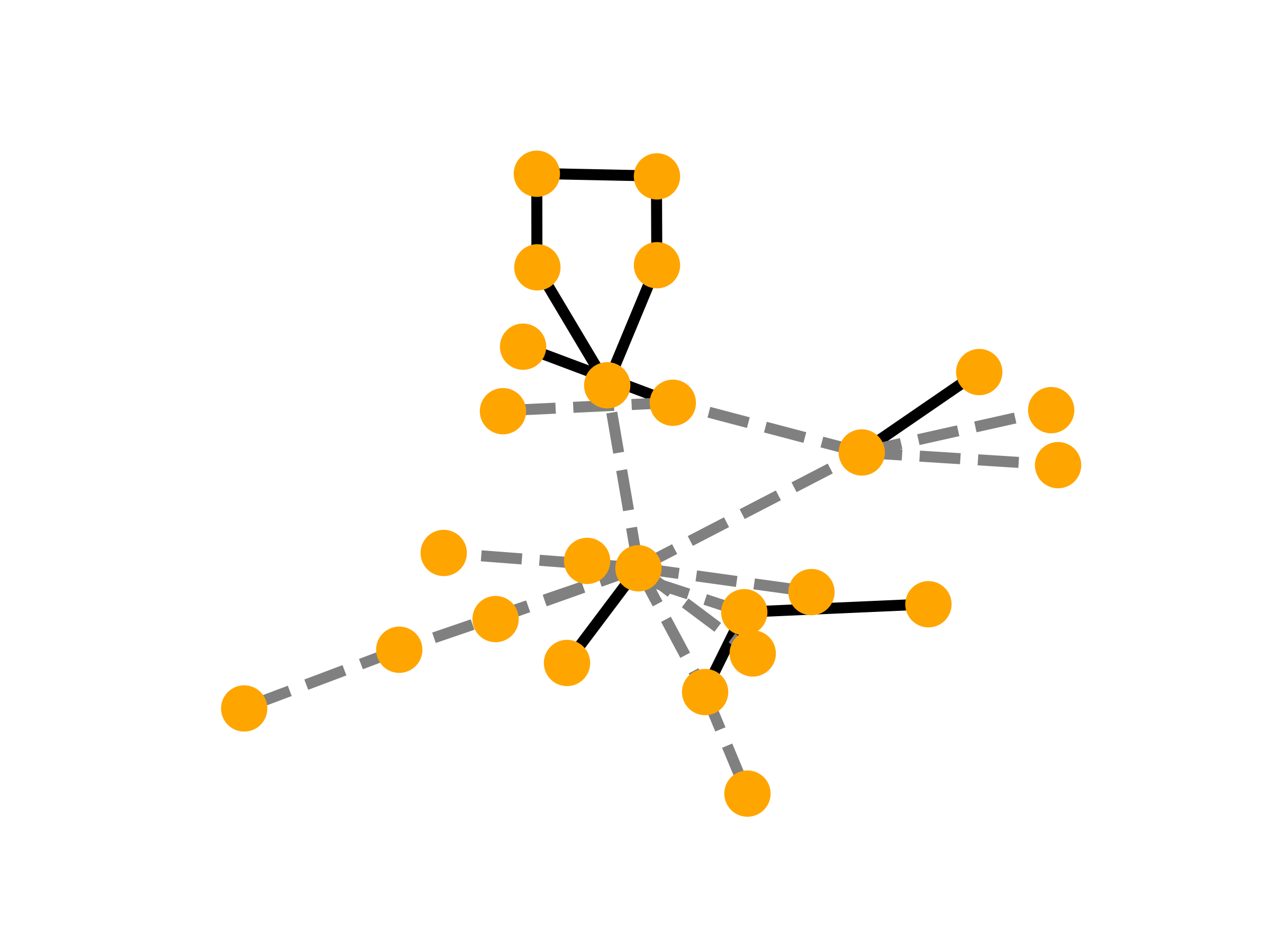
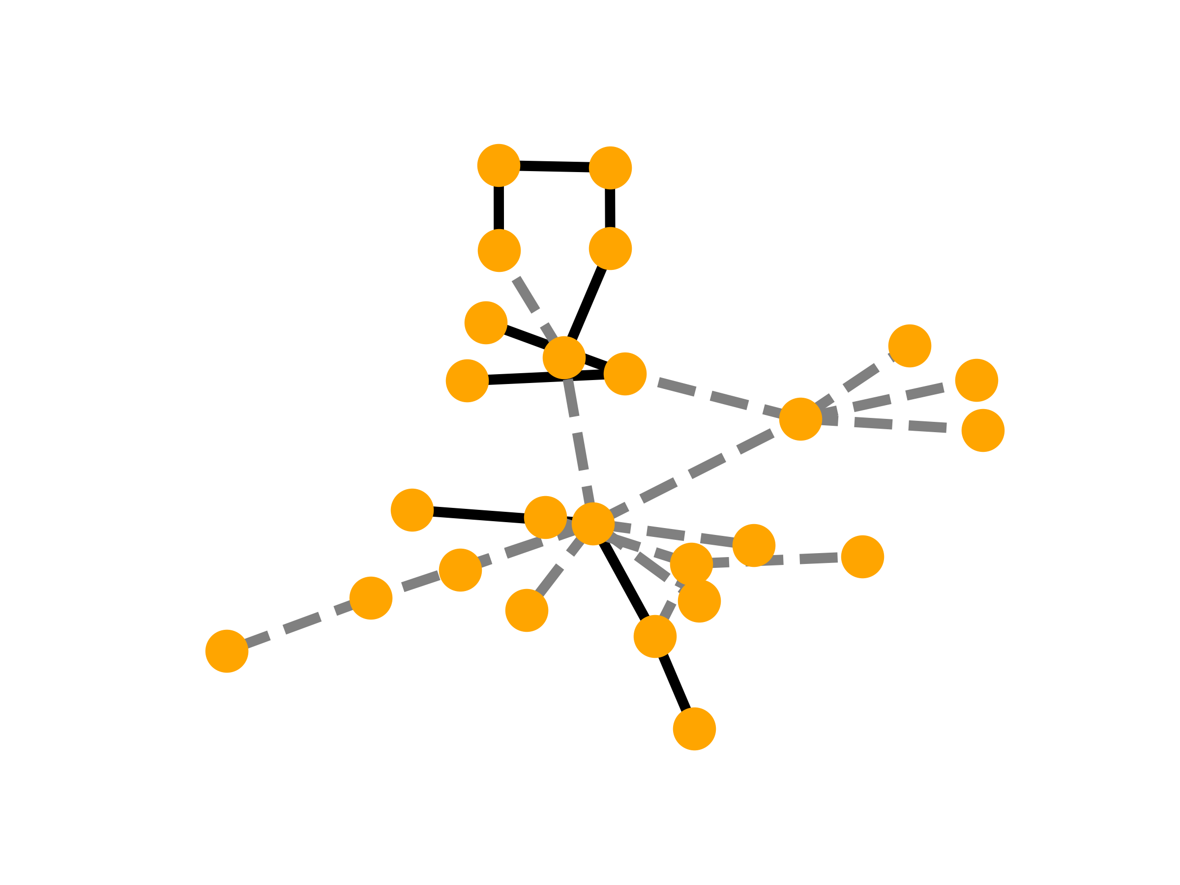
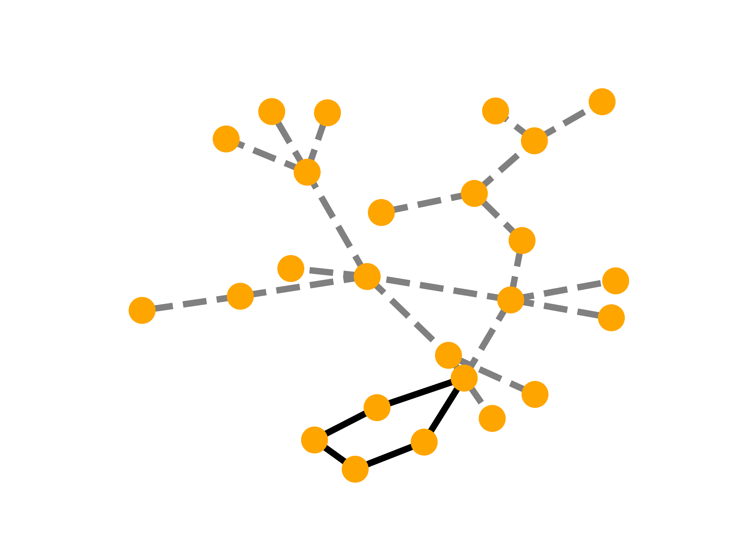
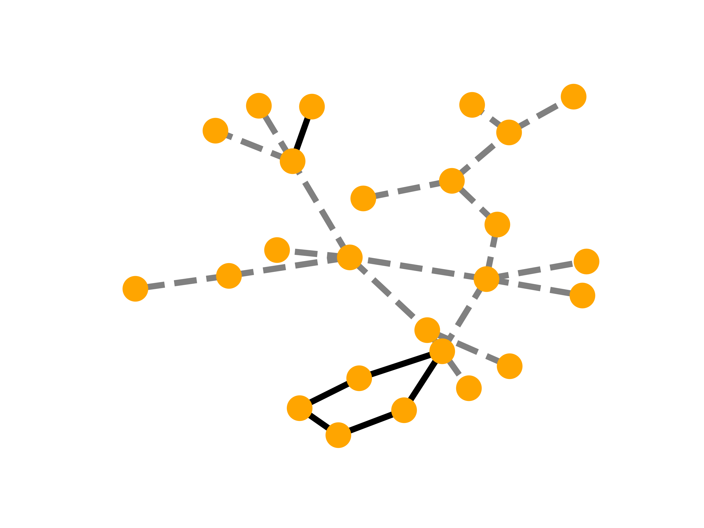
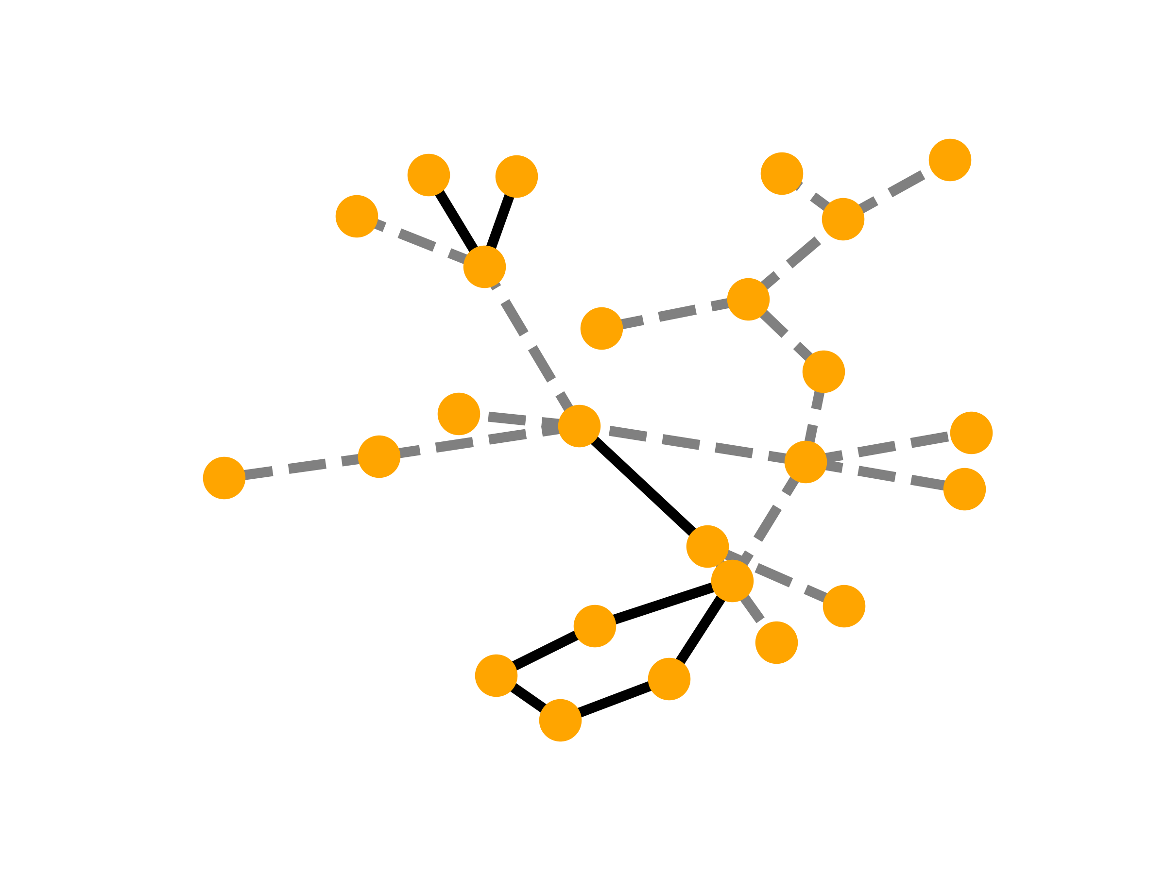
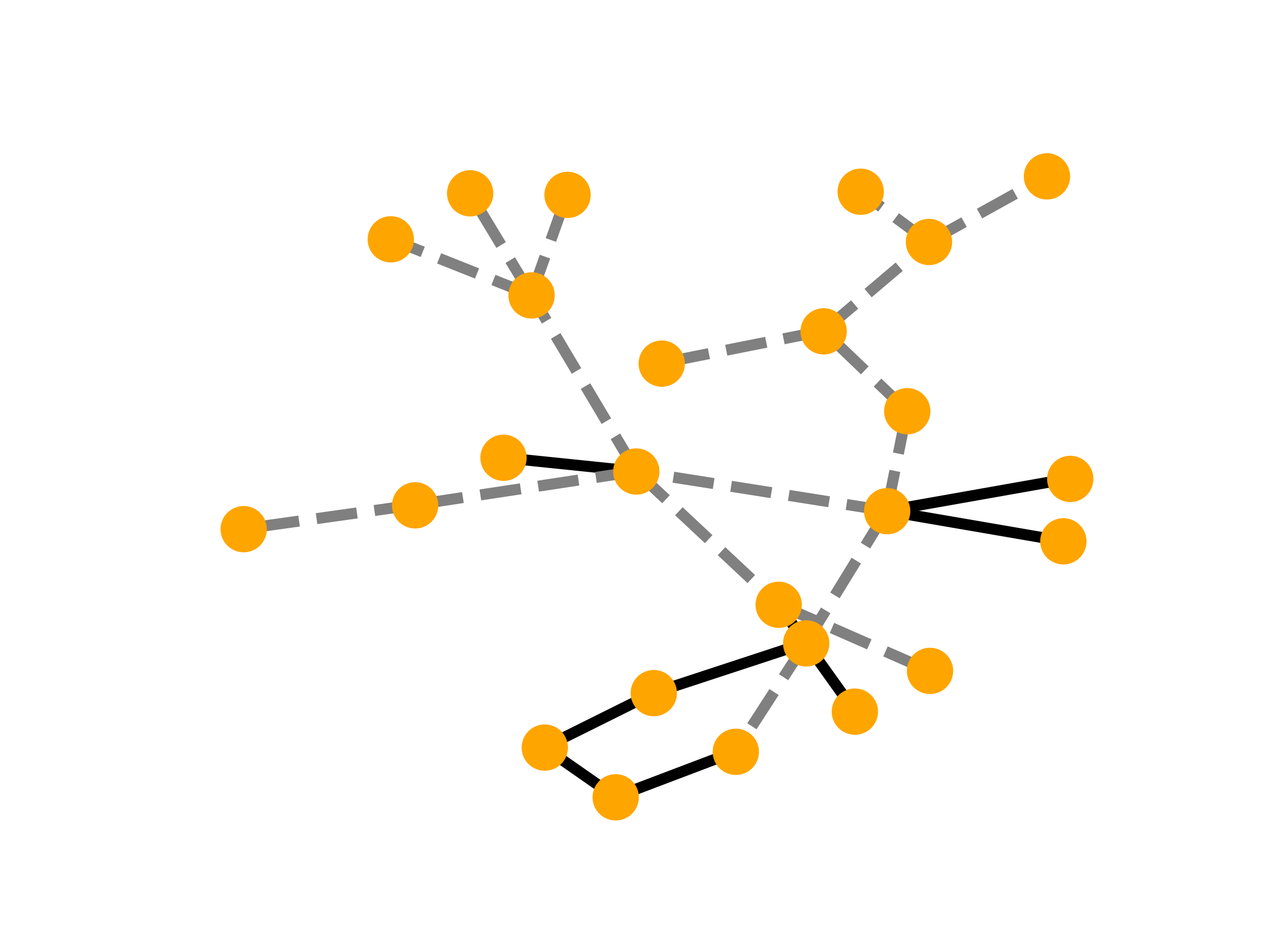
((a)) Ground Truth

((b)) ProxyExplainer

((c)) MixupExplainer

((d)) PGExplainer

((e)) GNNExplainer

Figure 11: Visualization of explanation on BA-2motifs.

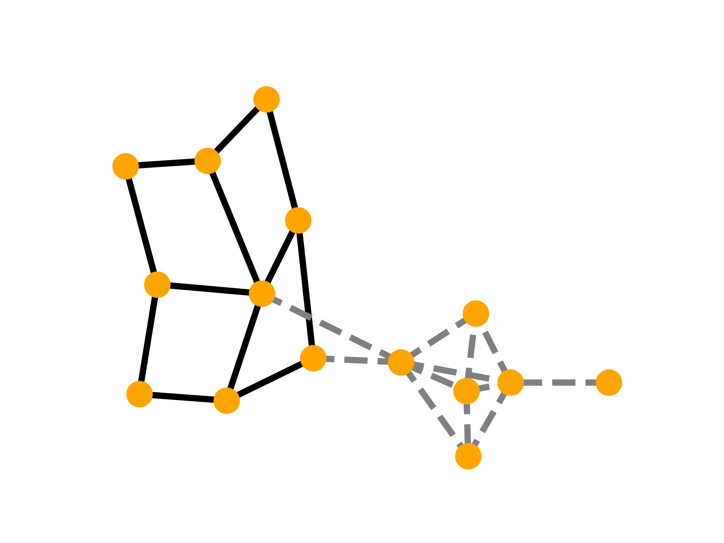
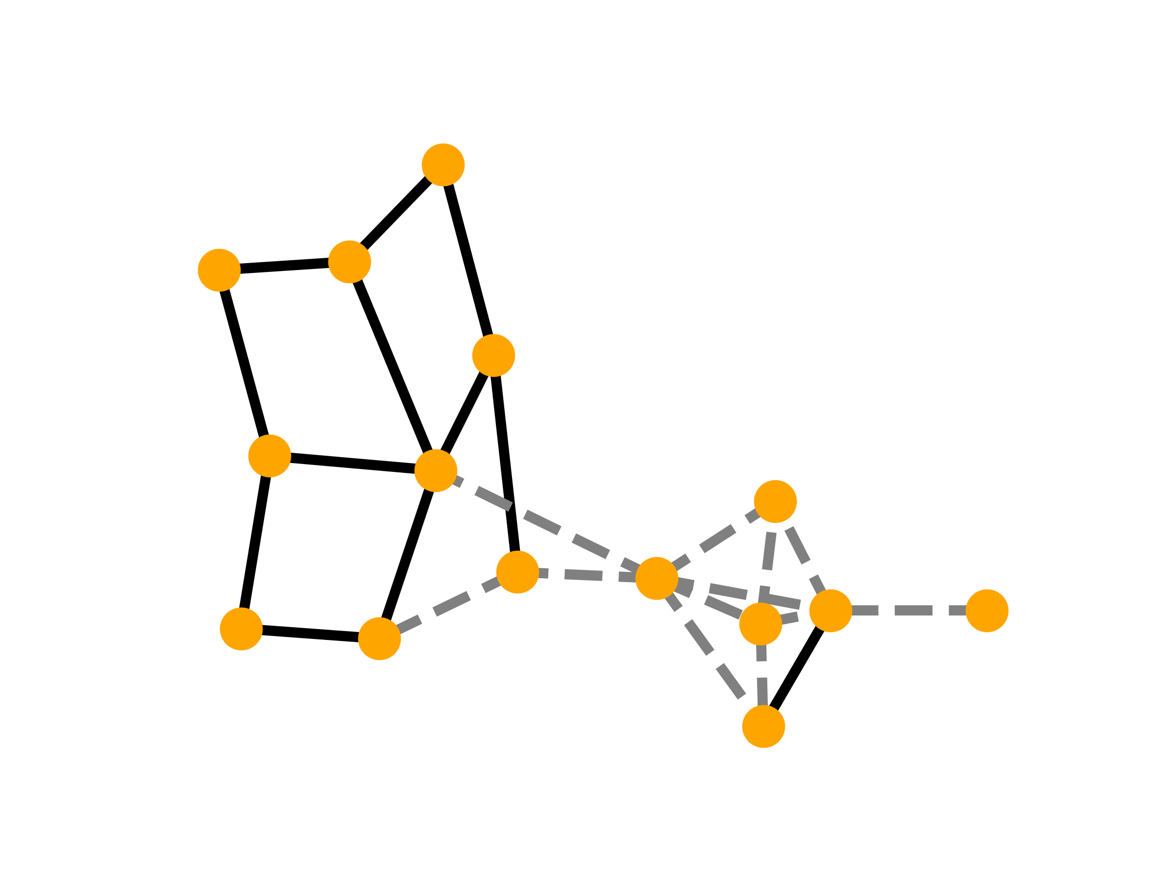
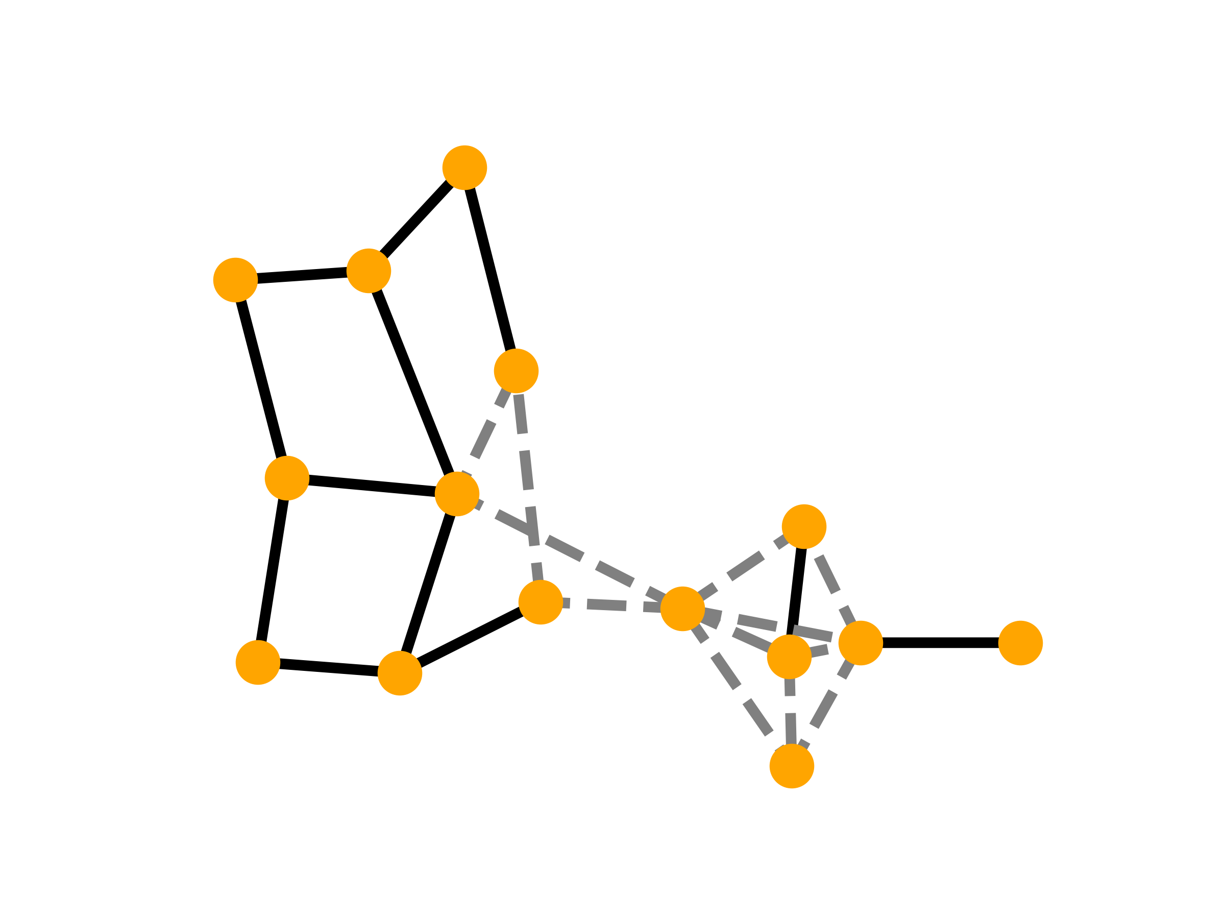
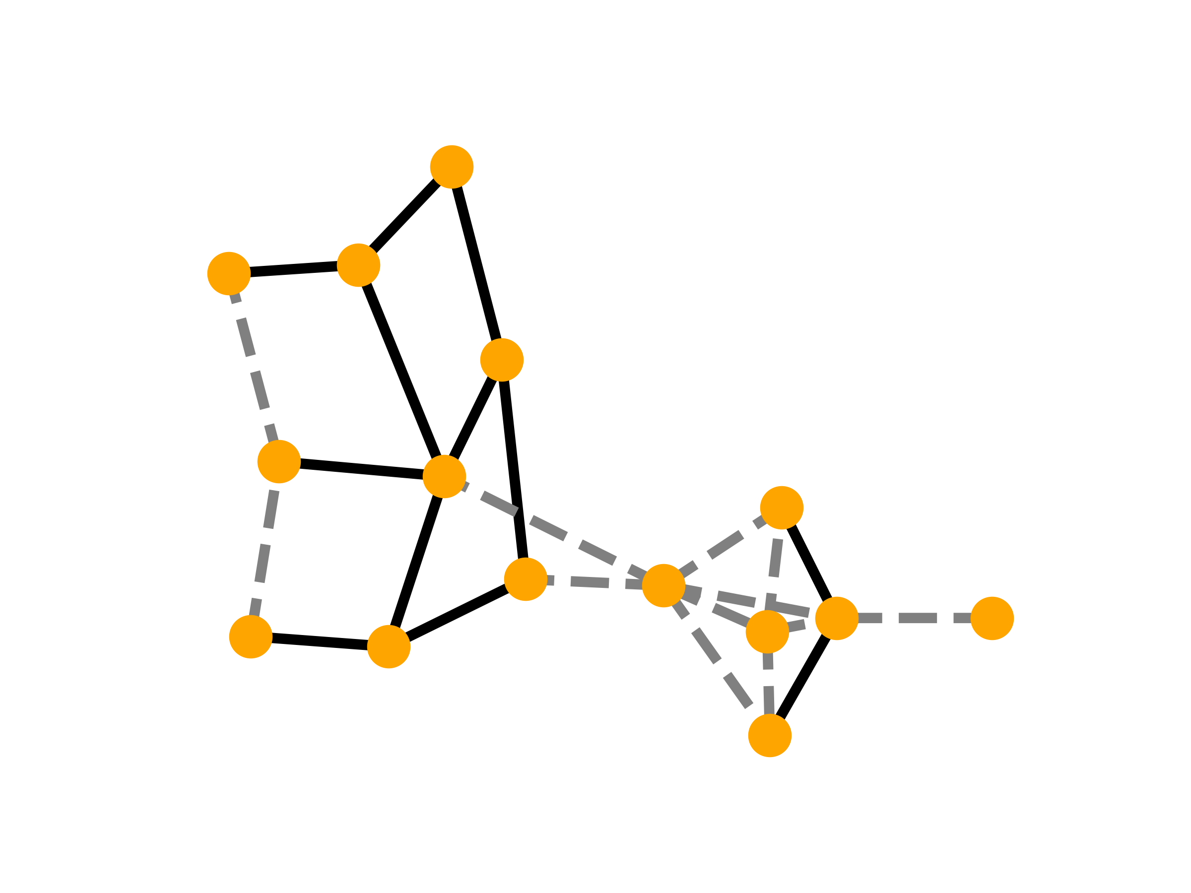
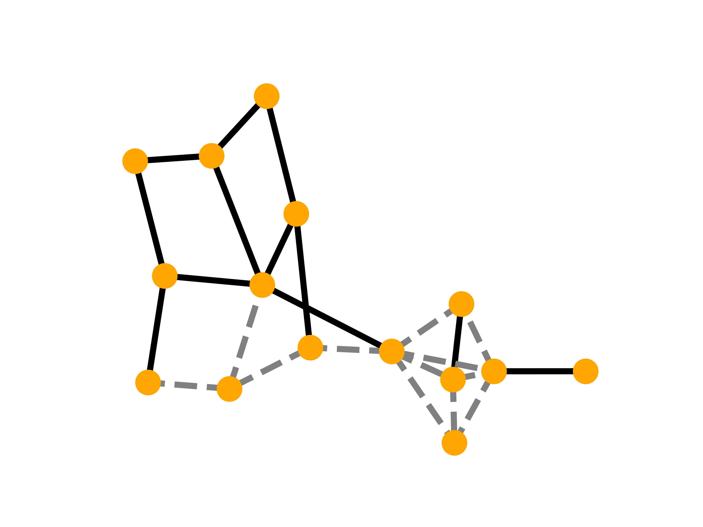
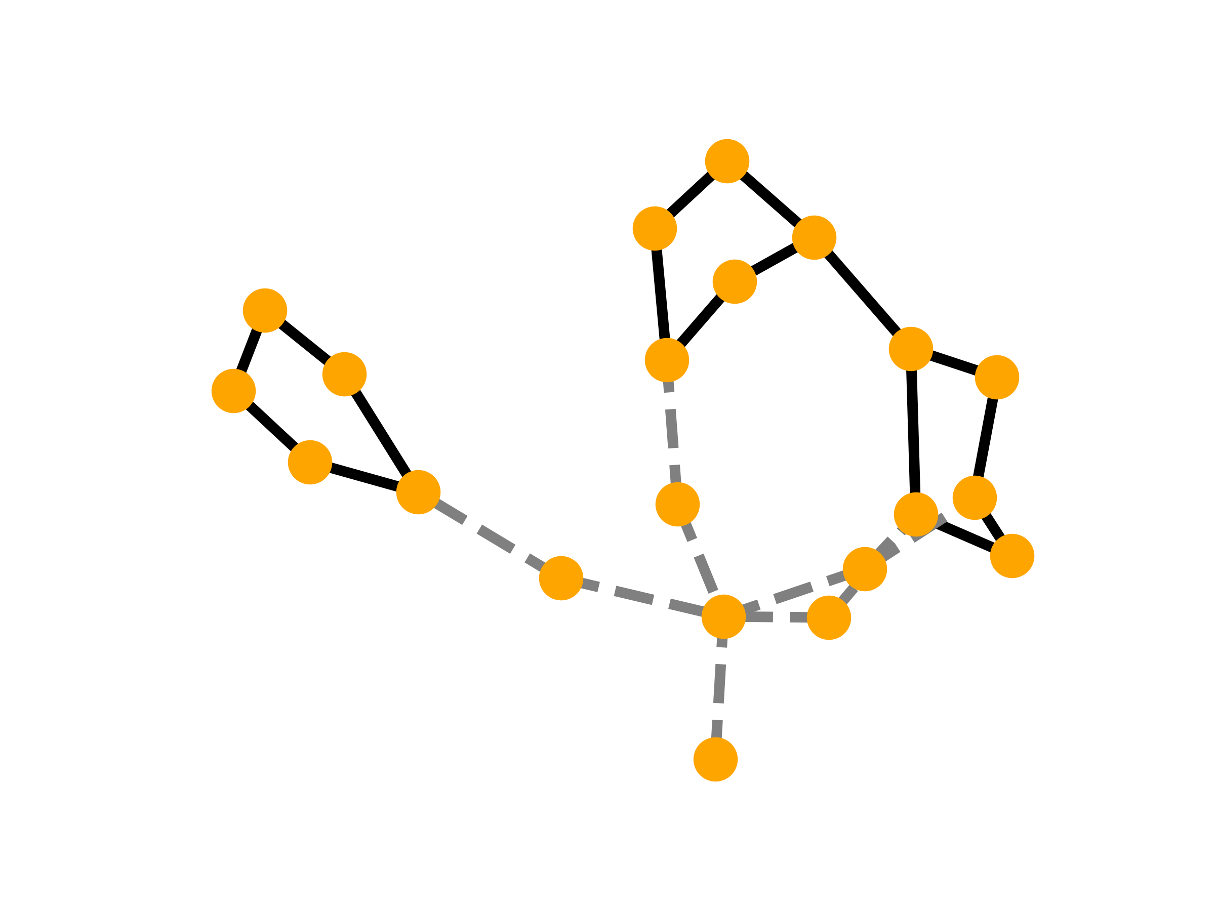
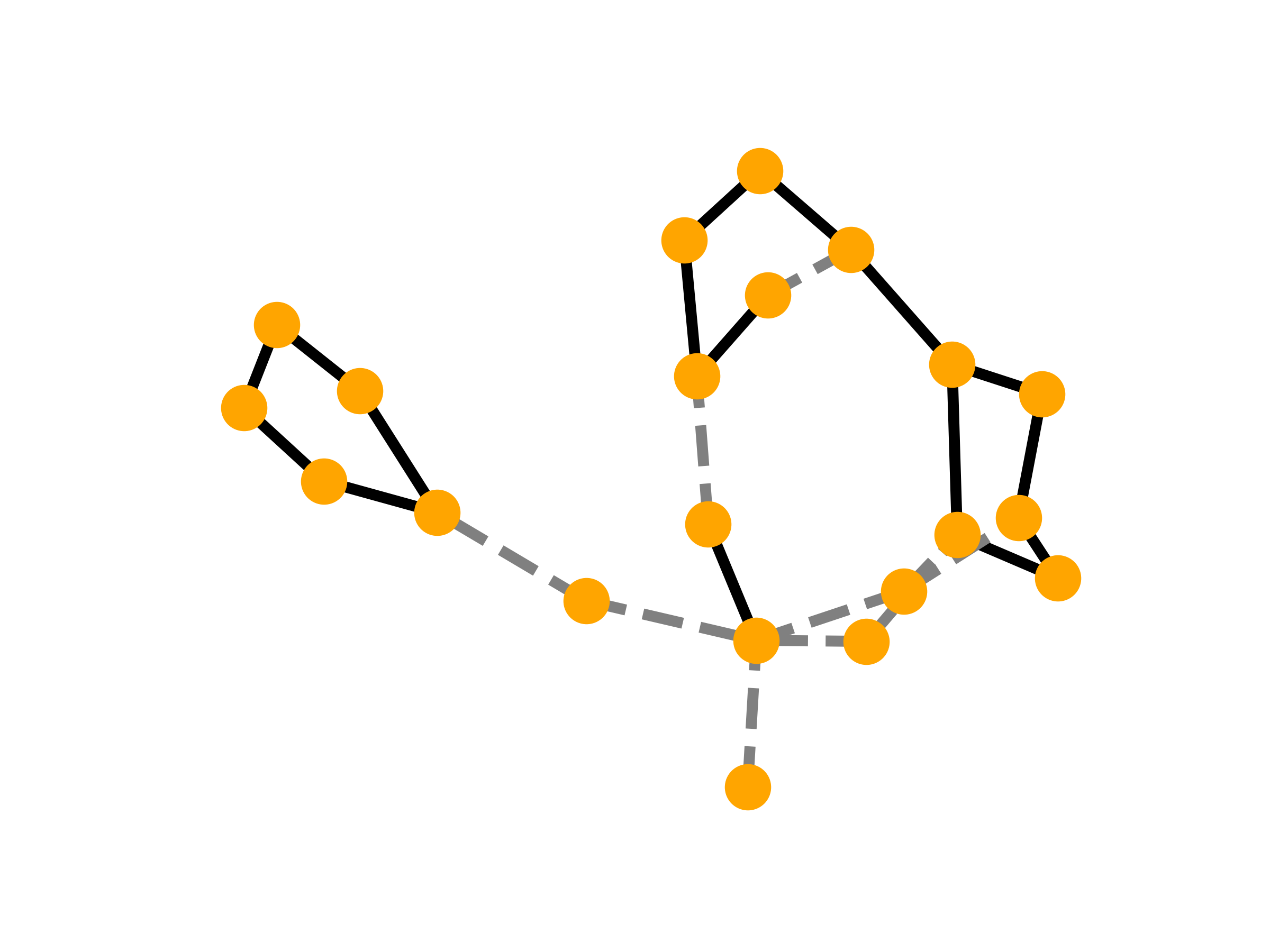
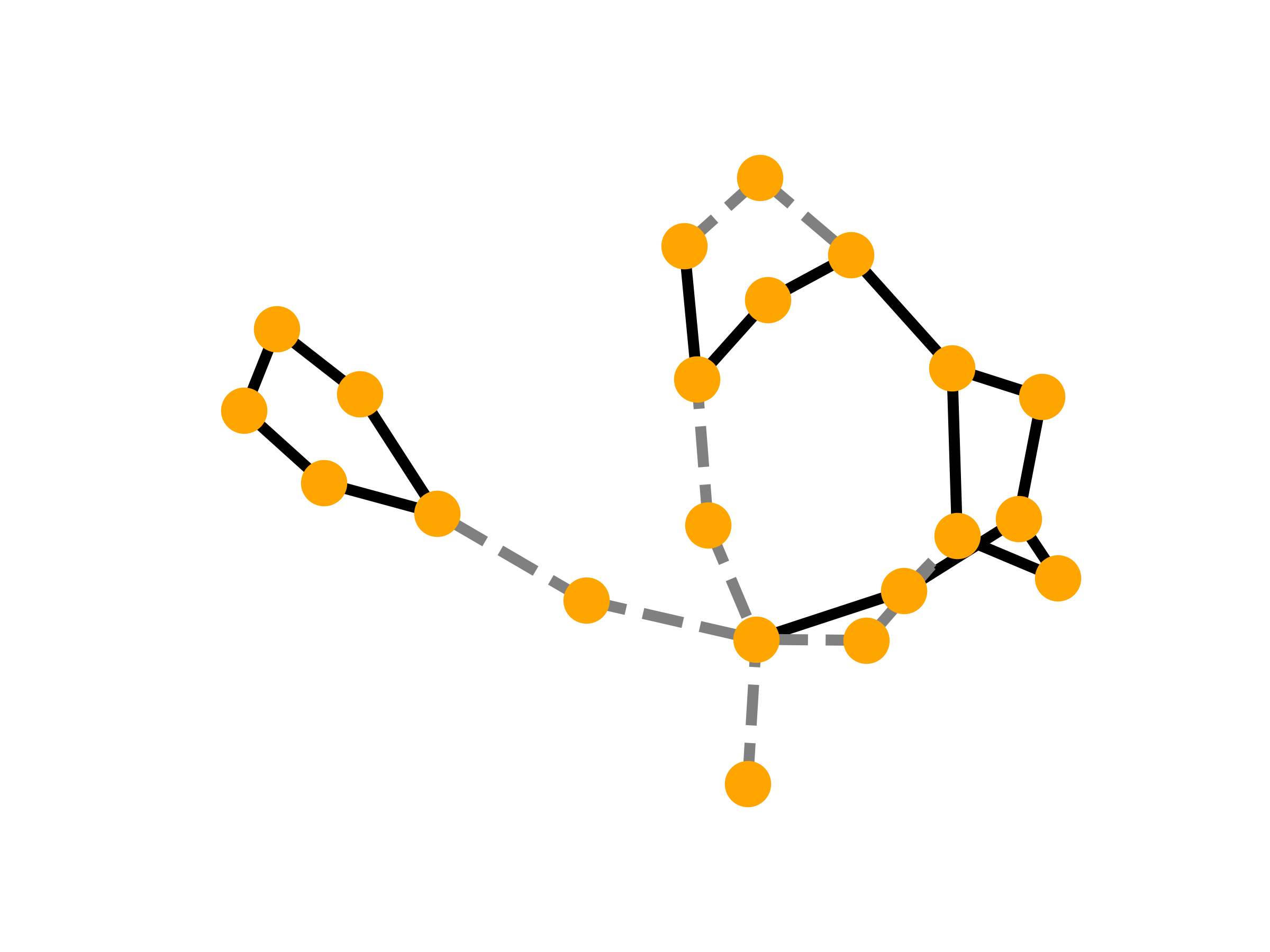
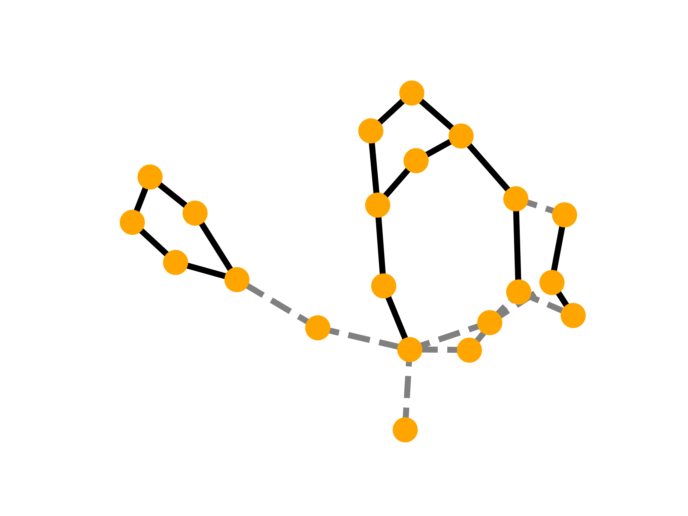
((a)) Ground Truth

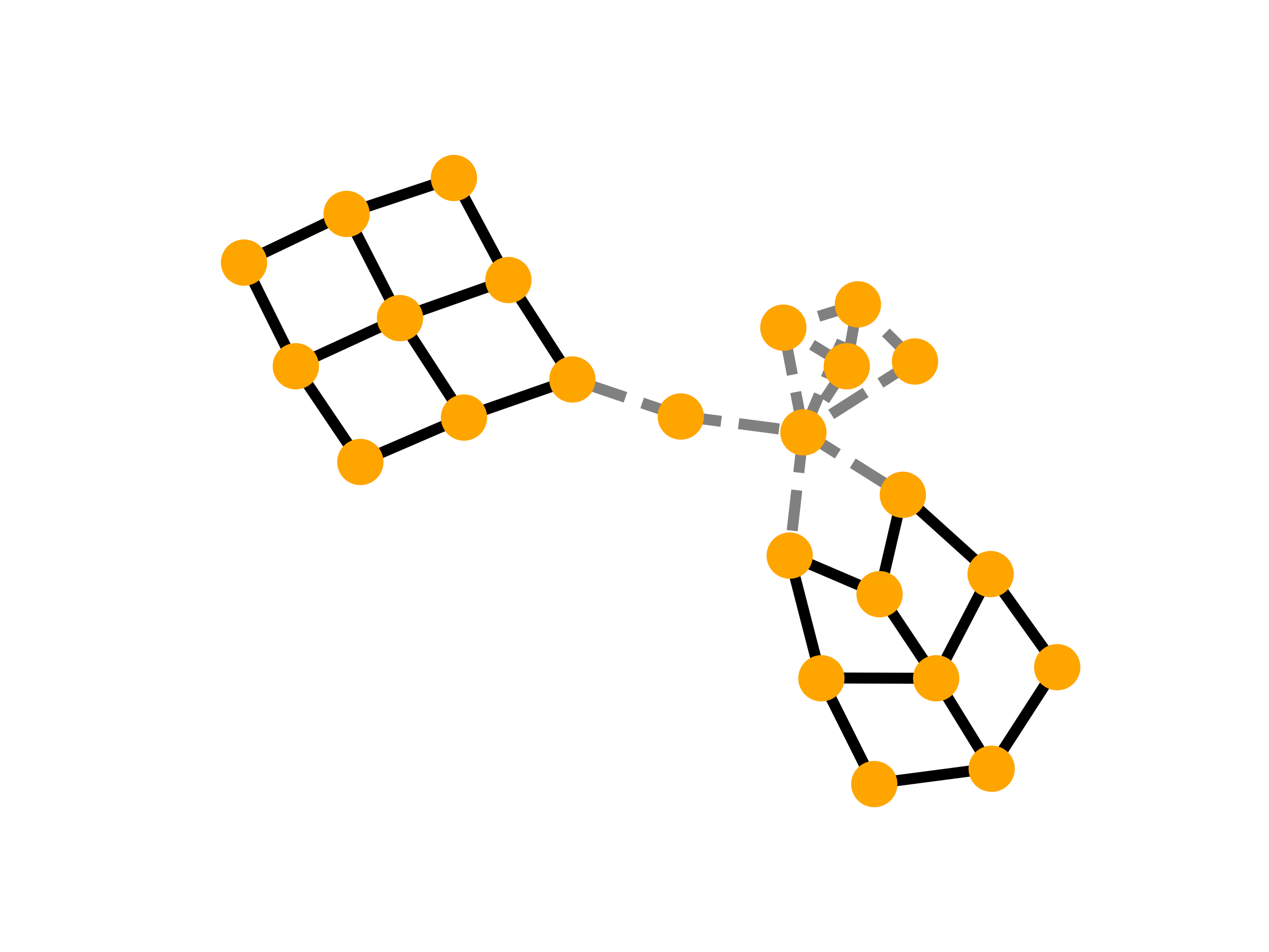
((b)) ProxyExplainer

((c)) MixupExplainer

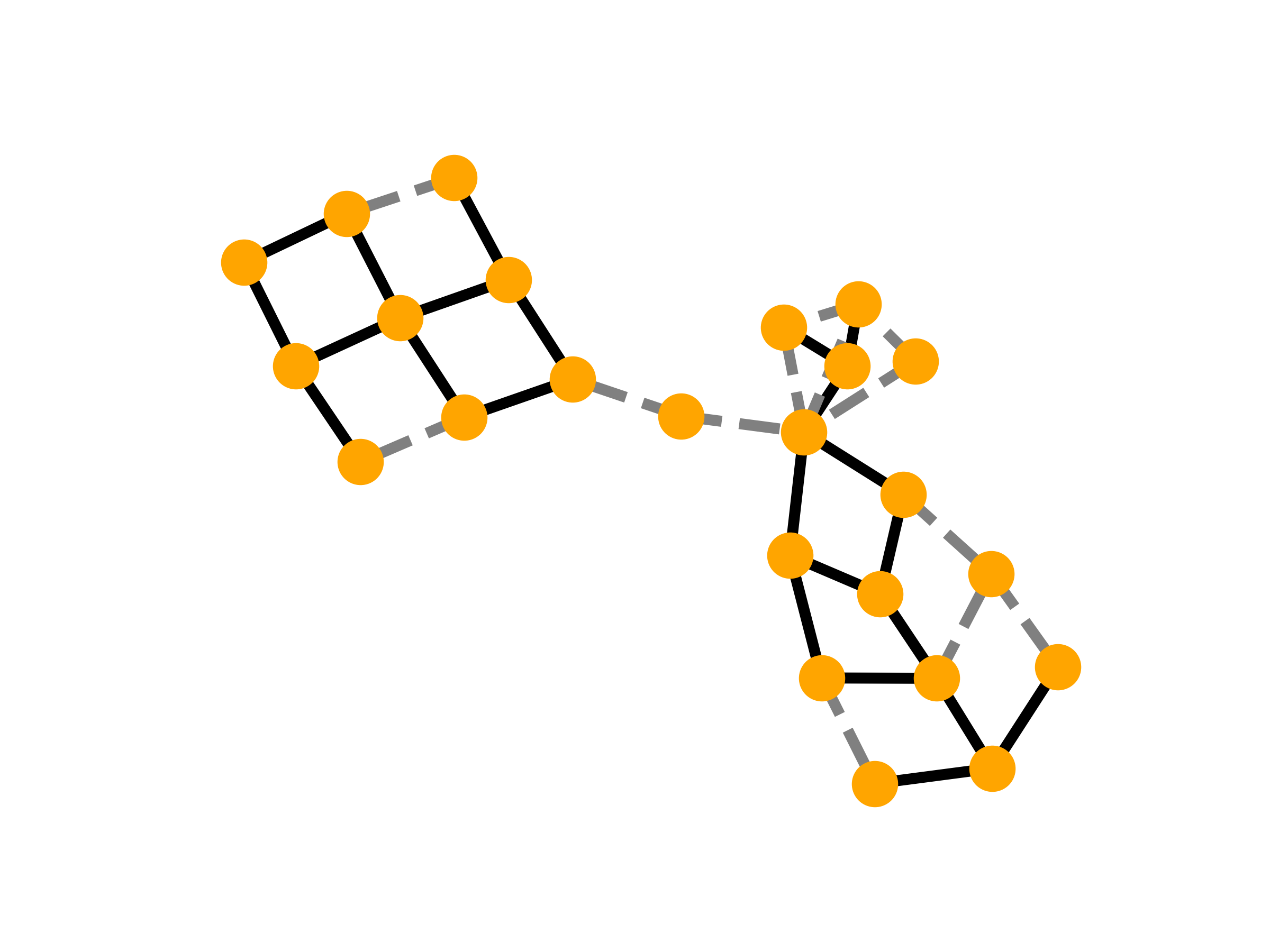
((d)) PGExplainer

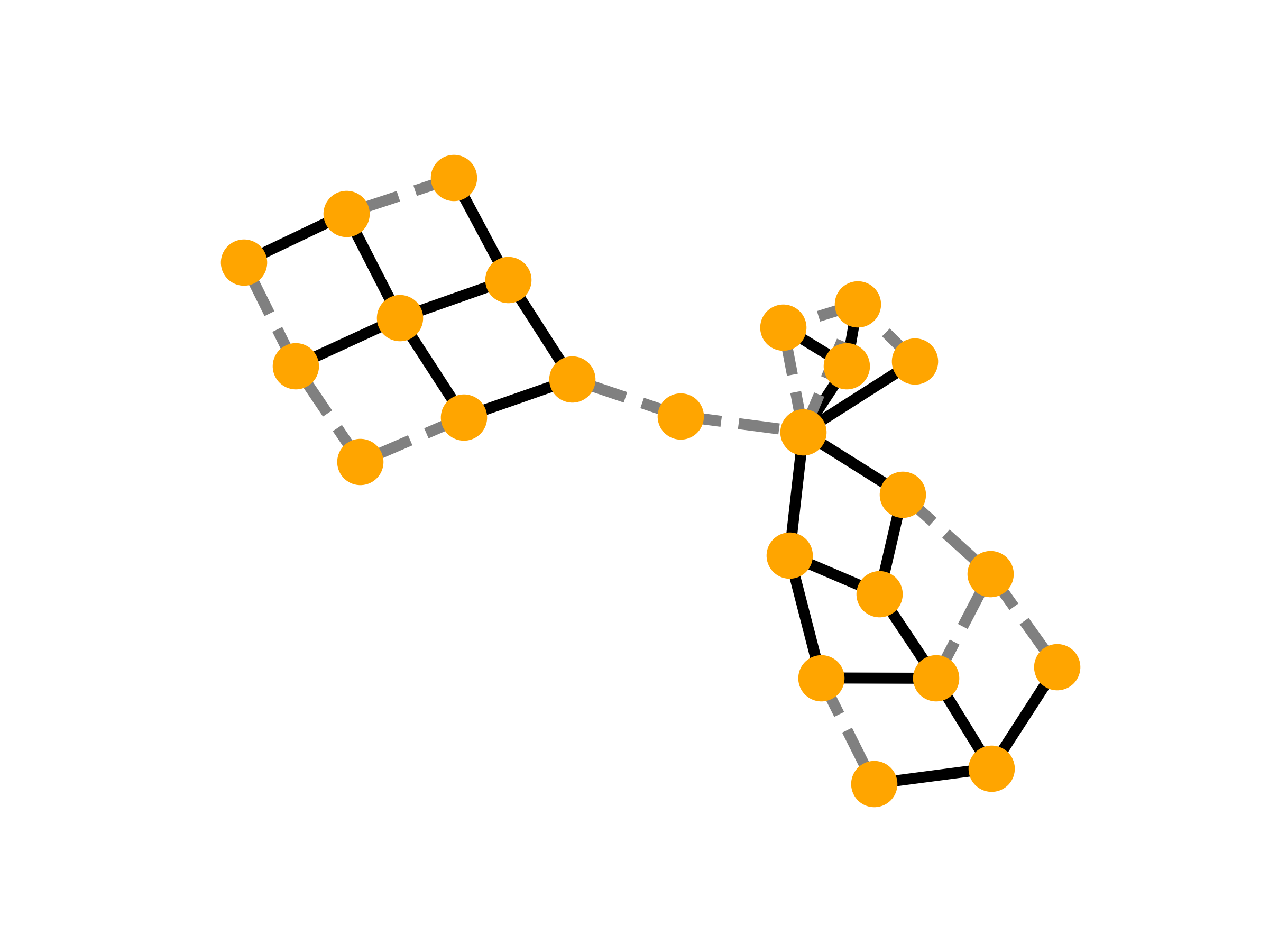
((e)) GNNExplainer

Figure 12: Visualization of explanation on BA-3motifs.

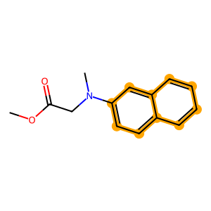
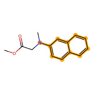
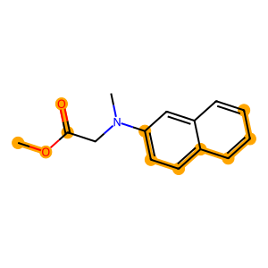
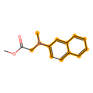
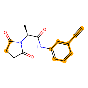
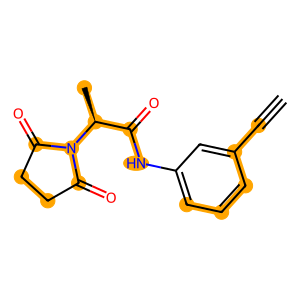
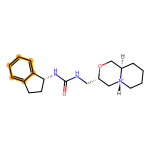
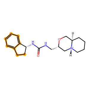
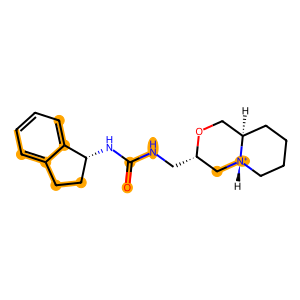
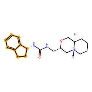
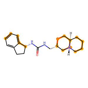
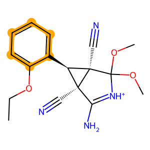
((a)) Ground Truth

((b)) ProxyExplainer

((c)) MixupExplainer

((d)) PGExplainer

((e)) GNNExplainer

Figure 13: Visualization of explanation on Benzene.

References

- Bank et al. (2023) Bank, D., Koenigstein, N., and Giryes, R. Autoencoders. Machine learning for data science handbook: data mining and knowledge discovery handbook, pp. 353–374, 2023.
- Chang et al. (2019) Chang, C.-H., Creager, E., Goldenberg, A., and Duvenaud, D. Explaining image classifiers by counterfactual generation. In International Conference on Learning Representations, 2019. URL https://openreview.net/forum?id=B1MXz20cYQ.
- Chen et al. (2023) Chen, J., Wu, S., Gupta, A., and Ying, Z. D4explainer: In-distribution explanations of graph neural network via discrete denoising diffusion. In Thirty-seventh Conference on Neural Information Processing Systems, 2023. URL https://openreview.net/forum?id=GJtP1ZEzua.
- Debnath et al. (1991) Debnath, A. K., Lopez de Compadre, R. L., Debnath, G., Shusterman, A. J., and Hansch, C. Structure-activity relationship of mutagenic aromatic and heteroaromatic nitro compounds. correlation with molecular orbital energies and hydrophobicity. Journal of medicinal chemistry, 34(2):786–797, 1991.
- Erdős et al. (1960) Erdős, P., Rényi, A., et al. On the evolution of random graphs. Publ. math. inst. hung. acad. sci, 5(1):17–60, 1960.
- Fang et al. (2023a) Fang, J., Liu, W., Gao, Y., Liu, Z., Zhang, A., Wang, X., and He, X. Evaluating post-hoc explanations for graph neural networks via robustness analysis. In Thirty-seventh Conference on Neural Information Processing Systems, 2023a.
- Fang et al. (2023b) Fang, J., Liu, W., Zhang, A., Wang, X., He, X., Wang, K., and Chua, T.-S. On regularization for explaining graph neural networks: An information theory perspective, 2023b. URL https://openreview.net/forum?id=5rX7M4wa2R_.
- Fang et al. (2023c) Fang, J., Liu, W., Zhang, A., Wang, X., He, X., Wang, K., and Chua, T.-S. On regularization for explaining graph neural networks: An information theory perspective, 2023c. URL https://openreview.net/forum?id=5rX7M4wa2R_.
- Fang et al. (2023d) Fang, J., Wang, X., Zhang, A., Liu, Z., He, X., and Chua, T.-S. Cooperative explanations of graph neural networks. In Proceedings of the Sixteenth ACM International Conference on Web Search and Data Mining, pp. 616–624, 2023d.
- Hamilton et al. (2017) Hamilton, W., Ying, Z., and Leskovec, J. Inductive representation learning on large graphs. Advances in neural information processing systems, 30, 2017.
- Huang et al. (2024) Huang, R., Shirani, F., and Luo, D. Factorized explainer for graph neural networks. In Proceedings of the AAAI conference on artificial intelligence, 2024.
- Jang et al. (2017) Jang, E., Gu, S., and Poole, B. Categorical reparameterization with gumbel-softmax. In International Conference on Learning Representations, 2017. URL https://openreview.net/forum?id=rkE3y85ee.
- Kazius et al. (2005) Kazius, J., McGuire, R., and Bursi, R. Derivation and validation of toxicophores for mutagenicity prediction. Journal of medicinal chemistry, 48(1):312–320, 2005.
- Kingma & Ba (2014) Kingma, D. P. and Ba, J. Adam: A method for stochastic optimization. arXiv preprint arXiv:1412.6980, 2014.
- Kipf & Welling (2017) Kipf, T. N. and Welling, M. Semi-supervised classification with graph convolutional networks. In International Conference on Learning Representations, 2017. URL https://openreview.net/forum?id=SJU4ayYgl.
- Li et al. (2023) Li, W., Li, Y., Li, Z., Hao, J., and Pang, Y. DAG matters! gflownets enhanced explainer for graph neural networks. In The Eleventh International Conference on Learning Representations, ICLR 2023, Kigali, Rwanda, May 1-5, 2023, 2023.
- Li et al. (2022) Li, Y., Zhou, J., Verma, S., and Chen, F. A survey of explainable graph neural networks: Taxonomy and evaluation metrics. arXiv preprint arXiv:2207.12599, 2022.
- Luo et al. (2020) Luo, D., Cheng, W., Xu, D., Yu, W., Zong, B., Chen, H., and Zhang, X. Parameterized explainer for graph neural network. Advances in neural information processing systems, 33:19620–19631, 2020.
- Maddison et al. (2017) Maddison, C. J., Mnih, A., and Teh, Y. W. The concrete distribution: A continuous relaxation of discrete random variables. In International Conference on Learning Representations, 2017. URL https://openreview.net/forum?id=S1jE5L5gl.
- Miao et al. (2022) Miao, S., Liu, M., and Li, P. Interpretable and generalizable graph learning via stochastic attention mechanism. In International Conference on Machine Learning, pp. 15524–15543. PMLR, 2022.
- Pope et al. (2019) Pope, P. E., Kolouri, S., Rostami, M., Martin, C. E., and Hoffmann, H. Explainability methods for graph convolutional neural networks. In Proceedings of the IEEE/CVF conference on computer vision and pattern recognition, pp. 10772–10781, 2019.
- Qiu et al. (2022) Qiu, L., Yang, Y., Cao, C. C., Zheng, Y., Ngai, H., Hsiao, J., and Chen, L. Generating perturbation-based explanations with robustness to out-of-distribution data. In Proceedings of the ACM Web Conference 2022, pp. 3594–3605, 2022.
- Sanchez-Lengeling et al. (2020) Sanchez-Lengeling, B., Wei, J., Lee, B., Reif, E., Wang, P., Qian, W., McCloskey, K., Colwell, L., and Wiltschko, A. Evaluating attribution for graph neural networks. Advances in neural information processing systems, 33:5898–5910, 2020.
- Sánchez-Lengeling et al. (2020) Sánchez-Lengeling, B., Wei, J. N., Lee, B. K., Reif, E., Wang, P., Qian, W. W., McCloskey, K., Colwell, L. J., and Wiltschko, A. B. Evaluating attribution for graph neural networks. In Advances in Neural Information Processing Systems 33: Annual Conference on Neural Information Processing Systems 2020, NeurIPS 2020, December 6-12, 2020, virtual, 2020.
- Scarselli et al. (2008) Scarselli, F., Gori, M., Tsoi, A. C., Hagenbuchner, M., and Monfardini, G. The graph neural network model. IEEE transactions on neural networks, 20(1):61–80, 2008.
- Sterling & Irwin (2015) Sterling, T. and Irwin, J. J. ZINC 15 - ligand discovery for everyone. J. Chem. Inf. Model., 55(11):2324–2337, 2015.
- Tishby et al. (2000) Tishby, N., Pereira, F. C., and Bialek, W. The information bottleneck method. arXiv preprint physics/0004057, 2000.
- Veličković et al. (2018) Veličković, P., Cucurull, G., Casanova, A., Romero, A., Liò, P., and Bengio, Y. Graph attention networks. In International Conference on Learning Representations, 2018. URL https://openreview.net/forum?id=rJXMpikCZ.
- Wang et al. (2016) Wang, D., Cui, P., and Zhu, W. Structural deep network embedding. In Proceedings of the 22nd ACM SIGKDD international conference on Knowledge discovery and data mining, pp. 1225–1234, 2016.
- Wang et al. (2021) Wang, X., Wu, Y., Zhang, A., He, X., and Chua, T. Towards multi-grained explainability for graph neural networks. In Advances in Neural Information Processing Systems 34: Annual Conference on Neural Information Processing Systems 2021, NeurIPS 2021, December 6-14, 2021, virtual, pp. 18446–18458, 2021.
- Wu et al. (2022) Wu, B., Li, J., Yu, J., Bian, Y., Zhang, H., Chen, C., Hou, C., Fu, G., Chen, L., Xu, T., et al. A survey of trustworthy graph learning: Reliability, explainability, and privacy protection. arXiv preprint arXiv:2205.10014, 2022.
- Wu et al. (2020) Wu, T., Ren, H., Li, P., and Leskovec, J. Graph information bottleneck. Advances in Neural Information Processing Systems, 33:20437–20448, 2020.
- Ying et al. (2019) Ying, Z., Bourgeois, D., You, J., Zitnik, M., and Leskovec, J. Gnnexplainer: Generating explanations for graph neural networks. Advances in neural information processing systems, 32, 2019.
- Yuan et al. (2022) Yuan, H., Yu, H., Gui, S., and Ji, S. Explainability in graph neural networks: A taxonomic survey. IEEE Transactions on Pattern Analysis and Machine Intelligence, 2022.
- Zhang et al. (2022a) Zhang, H., Wu, B., Yuan, X., Pan, S., Tong, H., and Pei, J. Trustworthy graph neural networks: Aspects, methods and trends. arXiv preprint arXiv:2205.07424, 2022a.
- Zhang et al. (2023a) Zhang, J., Chen, Z., Luo, D., Wei, H., et al. Regexplainer: Generating explanations for graph neural networks in regression tasks. In The Second Learning on Graphs Conference, 2023a.
- Zhang et al. (2023b) Zhang, J., Luo, D., and Wei, H. Mixupexplainer: Generalizing explanations for graph neural networks with data augmentation. In Proceedings of the 29th ACM SIGKDD Conference on Knowledge Discovery and Data Mining, pp. 3286–3296, 2023b.
- Zhang et al. (2022b) Zhang, S., Liu, Y., Shah, N., and Sun, Y. Gstarx: Explaining graph neural networks with structure-aware cooperative games. In Advances in Neural Information Processing Systems 35: Annual Conference on Neural Information Processing Systems 2022, NeurIPS 2022, New Orleans, LA, USA, November 28 - December 9, 2022, 2022b.
- Zheng et al. (2023) Zheng, X., Shirani, F., Wang, T., Cheng, W., Chen, Z., Chen, H., Wei, H., and Luo, D. Towards robust fidelity for evaluating explainability of graph neural networks. arXiv preprint arXiv:2310.01820, 2023.