Panacea: Pareto Alignment via Preference Adaptation for LLMs

Abstract

Current methods for large language model alignment typically use scalar human preference labels. However, this convention tends to oversimplify the multi-dimensional and heterogeneous nature of human preferences, leading to reduced expressivity and even misalignment. This paper presents Panacea, an innovative approach that reframes alignment as a multi-dimensional preference optimization problem. Panacea trains a single model capable of adapting online and Pareto-optimally to diverse sets of preferences without the need for further tuning. A major challenge here is using a low-dimensional preference vector to guide the model’s behavior, despite it being governed by an overwhelmingly large number of parameters. To address this, Panacea is designed to use singular value decomposition (SVD)-based low-rank adaptation, which allows the preference vector to be simply injected online as singular values. Theoretically, we prove that Panacea recovers the entire Pareto front with common loss aggregation methods under mild conditions. Moreover, our experiments demonstrate, for the first time, the feasibility of aligning a single LLM to represent a spectrum of human preferences through various optimization methods. Our work marks a step forward in effectively and efficiently aligning models to diverse and intricate human preferences in a controllable and Pareto-optimal manner.

1 Introduction

AI alignment aims to ensure AI systems align with human intentions, and there has been notable progress in this area, especially for large language models (LLMs) (Ji et al., 2023b; Casper et al., 2023; Kaufmann et al., 2023; Achiam et al., 2023). The prevailing approach for LLM alignment involves curating a dataset $\{(x,y_{1},y_{2},z)\}$, where each prompt $x$ is associated with a pair of responses $(y_{1},y_{2})$ and a scalar label $z\in\{0,1\}$ that indicates if $y_{1}$ is a “better” response. These labels are typically generated based on detailed guidelines that encompass various criteria, reflecting multiple dimensions $i\in\{1,\cdots,m\}$ of human preferences (e.g., helpfulness, harmlessness, conciseness, humor, formality). Pre-trained models are subsequently further optimized on this dataset using methods like reinforcement learning, supervised learning, or game-theoretical approaches (Jaques et al., 2019; Ouyang et al., 2022; Lee et al., 2023; Bai et al., 2022b; Rafailov et al., 2023; Azar et al., 2023; Swamy et al., 2024; Munos et al., 2023). However, this single-objective alignment methodology may not fully capture the complexity of real-world scenarios for two reasons (Figure 1).

First, this method can lead to inconsistency and ambiguity in the data labels. Human labelers assign scalar labels $z$ by implicitly evaluating responses across every dimension $i$, assigning varying preference weights to $i$, and reaching a final judgment. The inherently different preference weights between labelers often result in conflicting labels, causing misalignment or learning failures (analyzed in Appendix A). This challenge is underscored by the low average label agreement reported in (Bai et al., 2022a), a common issue in real-world scenarios.

Second, optimizing a single objective leads to only one model that attempts to fit the potentially conflicting labeling preferences, i.e., the helpfulness-harmlessness dilemma. This single model may not cover the full spectrum of human preferences across all dimensions, thereby exacerbating biases against underrepresented groups and failing to meet diverse user needs.

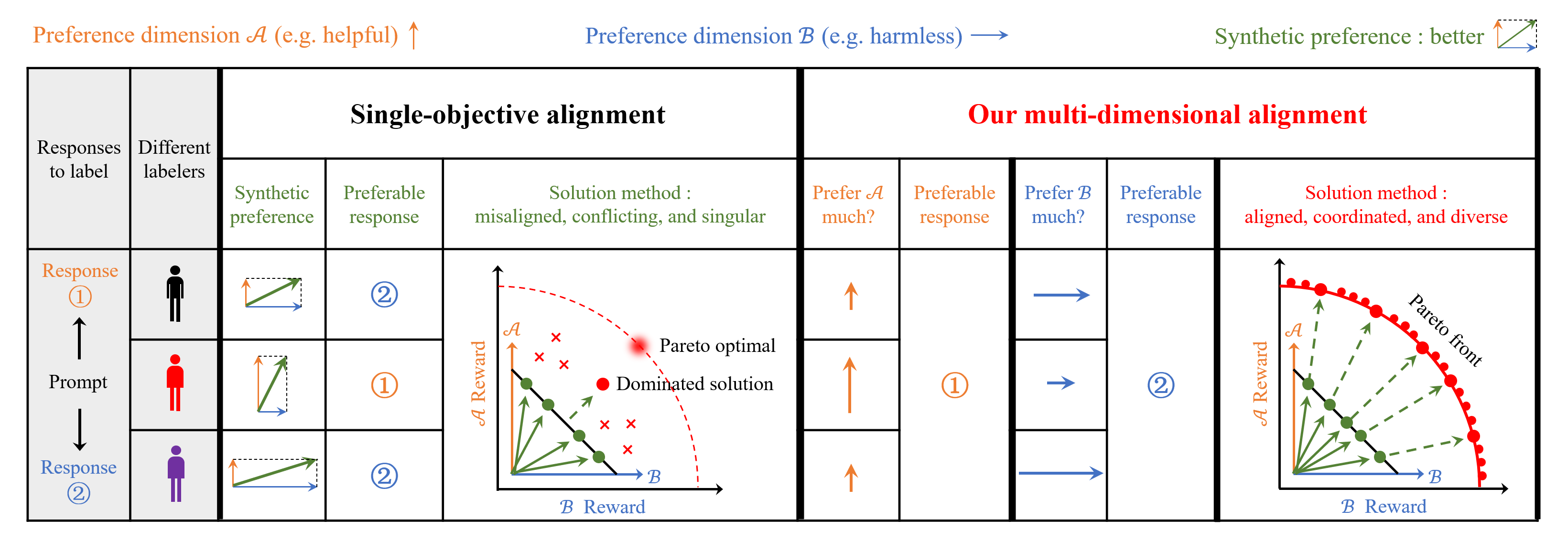
Figure 1: Comparison of the predominant single-objective alignment and our multi-dimensional alignment. For the two responses to a prompt, labelers agree on the preferable one in each preference dimension, but conflict when assigning a synthesized scalar label denoting which is “better”. This arises due to the inherently different preference weights held by labelers, a common case in reality. Performing single-objective optimization on the potentially conflicting scalar-label dataset (left) could lead to a dominated solution and misalignment. By contrast, our method, Panacea, leverages multi-dimensional preference optimization (right) on the consistent multi-dimensional dataset and learns the entire PF, thereby aligning with diverse and complex human preferences.

To address these challenges, we formulate the alignment as a multi-dimensional preference optimization (MDPO) problem. By explicitly assigning a label for each dimension, we enhance label consistency and simplify the labeling process, thereby overcoming the first limitation. Upon the obtained dataset, our goal is to concurrently optimize across all dimensions. However, this is often infeasible due to potential conflicts among preferences (e.g., helpfulness vs. harmlessness in response to hazardous user requests). Therefore, we aim for Pareto optimality and focus on learning the entire Pareto set. This method, providing a comprehensive representation of human preferences, effectively caters to diverse user needs, thus mitigating the second limitation (Figure 1).

In this paper, we propose Panacea (Pareto alignment via preference adaptation), a simple yet effective method that achieves two goals: 1) learning the entire Pareto-optimal solution set tailored to all possible preferences with one single model, and 2) online inferring Pareto-optimal responses by simply injecting any preference vector into the model.

A key challenge lies in how to utilize a low-dimensional preference vector to control the model’s behavior. Our core insight is that, similar to the crucial role of the preference vector in shaping the Pareto solution, singular values are pivotal in defining the model’s fundamental behavior in a singular value decomposition (SVD)-based low-rank adaptation (LoRA)(Hu et al., 2022; Zhang et al., 2023a). To address the above challenge, we incorporate the preference vector into the singular values within each SVD-LoRA layer. We then scale it using a learnable factor to align with the magnitude of other singular values. The model is trained end-to-end using a joint objective function aggregated according to the preference vector. The flexibility of Panacea enables seamless compatibility with various preference optimization procedures (e.g., RLHF and DPO) and diverse methods for loss aggregation (e.g., linear scalarization (LS) (Boyd & Vandenberghe, 2004)[Section 4.7.5] and weighted Tchebycheff (Tche) (Miettinen, 1999)[Section 3.4] ).

Our theoretical analysis demonstrates that, under practical conditions, Panacea with both LS and Tche aggregations can effectively capture the entire PF within the specific DPO and RLHF frameworks. This finding provides a solid rationale for training a single Pareto set model to learn all Pareto optimal solutions across the entire preference space.

In our experiments, we apply Panacea to address the classic helpfulness-harmlessness dilemma in alignment. Specifically, Panacea successfully learns the complete Pareto set for diverse preferences using the BeaverTails dataset (Ji et al., 2023a). It consistently outperforms alternative methods across various optimization techniques and loss aggregation methods, while being significantly more computationally efficient. Additionally, Panacea forms a smooth convex PF that aligns best with theoretical expectations compared to baselines. For the first time, we show the possibility of aligning a single model with heterogeneous preferences, opening up a promising avenue for LLM alignment.

This paper makes three main contributions. First, we identify the fundamental limitations of the predominant scalar-label, single-objective alignment paradigm, and propose to reframe alignment as a multi-dimensional preference optimization problem. Second, we design Panacea, a simple yet effective method that learns one single model that can online and Pareto-optimally adapt to any set of preferences, without the need for further tuning. Third, we provide theoretical supports and empirical validations to demonstrate the Pareto optimality, effectiveness, efficiency, and simplicity of Panacea, thereby satisfying the urgent need for Pareto alignment to diverse human preferences.

2 Related Work and Preliminaries

2.1 Pareto Set Learning

Different from previous classical multi-objective optimization (MOO) methods (Zhou et al., 2011; Lin et al., 2019; Liu et al., 2021; Zhang & Li, 2007) that use a finite set of solutions (referred to as “particles”) to approximate the entire Pareto set, Pareto set learning (PSL) (Navon et al., 2020; Lin et al., 2020; Zhang et al., 2023b) aims to use a single model to recover the complete Pareto set/front. The advantage of PSL is that it can store an infinite number of Pareto solutions within a model. This allows users to specify their own preferences, and the model can dynamically output a particular Pareto solution in real-time according to those preferences. Typical applications of PSL includes multiobjective industrial design problems (Zhang et al., 2023b; Lin et al., 2022), reinforcement learning (Basaklar et al., 2022; Yang et al., 2019; Hwang et al., 2023), text-to-image generalization (Lee et al., 2024), and drug design (Jain et al., 2023; Zhu et al., 2023). While there have been some studies on PSL involving deep neural networks, these models are considerably smaller compared to LLMs. Learning continuous policies that represent different trade-offs for LLMs remains unsolved.

2.2 Single-Objective Preference Optimization

In recent years, large language models such as ChatGPT (John Schulman & Hilton, 2022), GPT-4 (Achiam et al., 2023), and Claude (Anthropic, 2023) have demonstrated remarkable text generation capabilities that align with human preferences. This performance is achieved by fine-tuning these models using alignment techniques. Popular alignment methods can be categorized into two categories. The first category optimizes reward models learned from single-dimensional human preference labels. Works in this category include RLHF (Ouyang et al., 2022), which uses reinforcement learning for optimization, and RRHF (Yuan et al., 2023), which employs supervised learning for optimization, as well as RAFT (Dong et al., 2023a) and other similar approaches. The second category directly utilizes single-dimensional human-annotated preference labels for optimization, circumventing the learning of reward models. Representative works include DPO (Rafailov et al., 2023), establishing a mapping between the reward function and the optimal strategy for direct policy optimization, and NLHF (Munos et al., 2023) and SPO (Swamy et al., 2024), introducing game theory for preference optimization based on preference models. These works aim to align the model with scalar preference labels indicating which response is considered “better”. In essence, all these approaches model the alignment problem of large language models as a single-objective optimization problem.

Taking RLHF as an example, RLHF first captures human preferences in the form of a reward model $r(x,y)$, where $x$ is a prompt and $y$ is a response, and then performs PPO to maximize the obtained reward with KL regularization to penalize large deviation from the original supervised fine-tuned model $\pi_{\text{ref}}$, according to the following reinforcement learning objective:

$$\max_{\theta}J_{\text{RLHF}}(\pi_{\theta})=\max_{\theta}\ \mathbb{E}_{x\sim\mathcal{D},y\sim\pi_{\theta}(y|x)}\left[r(x,y)\right]$$

$$- \beta\mathbb{D}_{\text{KL}}\left[\pi_{\theta}(y|x)||\pi_{\text{ref}}(y|x)\right].$$ (1)

DPO simplifies RLHF procedure by directly optimizing the human preference with the language model, thus obtaining a supervised learning objective:

$$\min_{\theta}\mathcal{L}_{\text{DPO}}(\pi_{\theta})$$

$$= \min_{\theta}-\mathbb{E}\left[\log\sigma\left(\beta\log\frac{\pi_{\theta}\left(y_{w}|x\right)}{\pi_{\mathrm{ref}}\left(y_{w}|x\right)}-\beta\log\frac{\pi_{\theta}\left(y_{l}|x\right)}{\pi_{\mathrm{ref}}\left(y_{l}|x\right)}\right)\right],$$ (2)

where the expectation is over $(x,y_{w},y_{l})\sim\mathcal{D}$.

2.3 Multi-Dimensional Preference Optimization

Before our work, several previous attempts have been made to learn policies with multi-dimensional objectives for alignment. In the RL settings, AlignDiff (Dong et al., 2023b) trains an attribute-conditioned diffusion model to conduct preference alignment planning. In LLM, MORE (MultiObjective REward model) (Zeng et al., 2023) addresses the challenge of balancing multi-dimensional objectives using the Multiple Gradient Descent Algorithm (MGDA) (Désidéri, 2012). However, this paper has some unresolved issues. For example, the MGDA-based method can only recover a single Pareto optimal solution at a time and its results are heavily influenced by different initializations (Sener & Koltun, 2018; Lin et al., 2019). Furthermore, MORE solely trains a reward model with varying trade-offs and does not fully solve the problem of dimensional reward alignment. Rewarded Soups (RS) (Rame et al., 2023) is an alternative method to learn Pareto optimal LLM models. RS learns a model for each dimension and combines their parameters linearly to generate a new Pareto optimal model. While RS is simple, ensuring the accuracy of the interpolated model poses a challenge. In contrast, Panacea is more powerful because it only embeds preference vectors into LLM to more accurately recover PF under any preference vector.

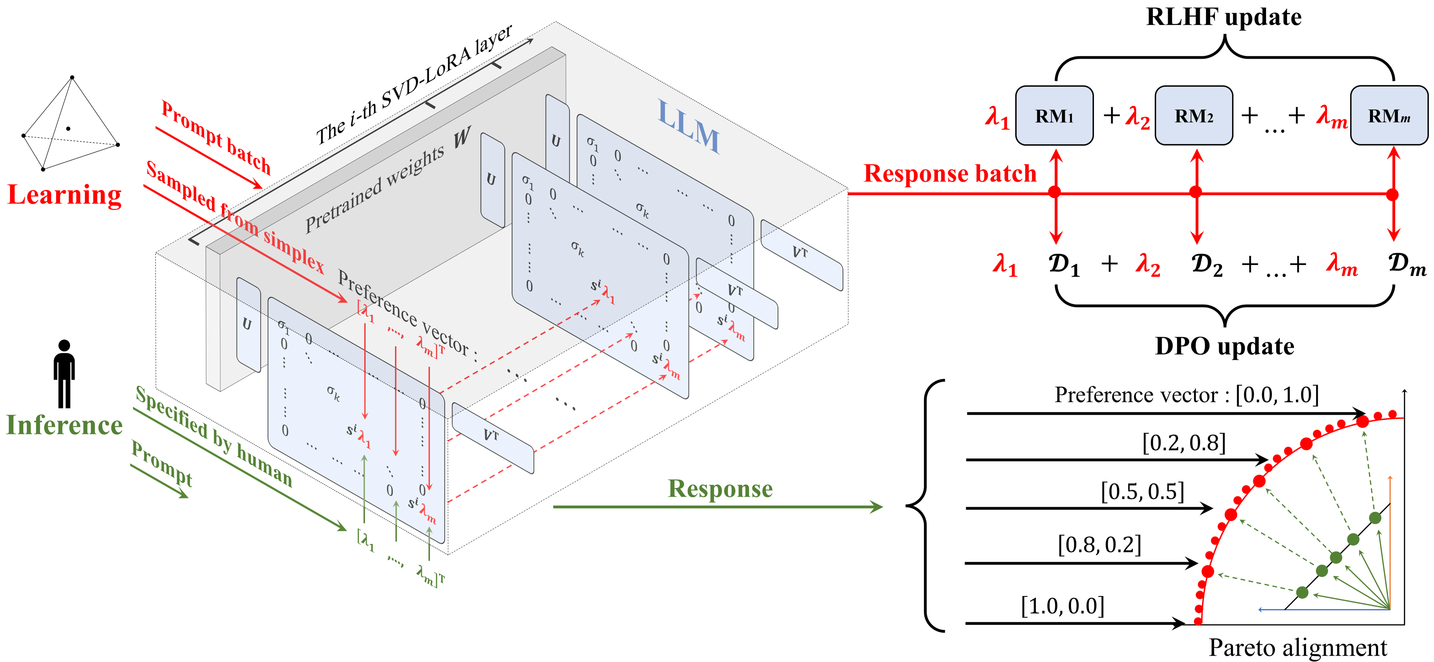
Figure 2: Visual illustration of Panacea. Panacea innovatively embeds the preference vector into singular values of each SVD-LoRA layer and scales it with learnable factors to match the magnitudes. During learning, for each data batch, we randomly sample a preference vector from the preference simplex and train the embedded model with various optimization procedures and loss aggregation methods. In the inference stage, the model adapts online to the user-specified preference vector and exhibits Pareto alignment in its responses.

3 Problem Formulation

Human preference is inherently multi-dimensional. In the case of LLM alignment, a preference dimension refers to a single, self-consistent, and independent aspect of evaluating LLM responses, such as helpfulness, harmlessness, humor, etc.. We formulate the multi-dimensional preference optimization (MDPO) problem with $m$ dimensions as:

$$\max_{\theta\in\Theta}{\bm{J}}(\pi_{\theta})=(J_{1}(\pi_{\theta}),J_{2}(\pi_{\theta}),\ldots,J_{m}(\pi_{\theta})),$$ (3)

where $\pi_{\theta}\in\Pi$ is a policy, i.e. an LLM, and $\theta$ is its trainable parameters (decision variable), $\Pi$ is the policy space, $\Theta$ is the parameter space, and $J_{i},i=1,\cdots,m$ denotes a performance measure of dimension $i$, such as $J_{\text{RLHF},i}(\pi_{\theta})$ and $-\mathcal{L}_{\text{DPO},i}(\pi_{\theta})$. Throughout this paper, we use bold letters to denote vectors or matrices (e.g. $\bm{J},{\bm{\lambda}}$). Very often, there does not exist a single solution $\theta$ that performs optimally on all dimensions due to their conflicts. Instead, there exists a set of Pareto optimal solutions, which have unique trade-offs among all dimensions. We say solution $\theta^{(a)}$ dominates $\theta^{(b)}$, denoted as $\bm{J}(\pi_{\theta^{(a)}})\succ{\bm{J}}(\pi_{\theta^{(b)}})$, if for all $i\in[m]$, $J_{i}(\pi_{\theta^{(a)}})\geq J_{i}(\pi_{\theta^{(b)}})$, and there exists at least one index $j\in[m]$ such that $J_{j}(\pi_{\theta^{(a)}})>J_{j}(\pi_{\theta^{(b)}})$ (Ehrgott, 2005; Miettinen, 1999). Based on this definition, we provide definitions for Pareto optimality.

Definition 3.1 (Pareto optimality).

We call a solution $\theta^{*}$ Pareto optimal if no other solution $\theta^{\prime}\in\Theta$ dominates $\theta^{*}$. The set of all Pareto optimal solutions is called the Pareto set (PS); while its image set in the objective space is called the PF, ${\mathcal{F}^{*}}$.

For theoretical completeness, we introduce the concept of a weakly Pareto optimal solution. A solution $\theta^{*}$ is considered weakly Pareto optimal if no other solution $\theta^{\prime}$ can strictly dominate it, that is, if $J_{i}(\pi_{\theta^{\prime}})>J_{i}(\pi_{\theta^{*}})$ for all $i\in[m]$.

Human’s trade-offs among all dimensions are quantified as a preference vector, $\bm{\lambda}=(\lambda_{1},\ldots,\lambda_{m})$, where $\bm{\lambda}\in\Delta_{m-1}$, $\lambda_{i}\geq 0$, and $\sum_{i=1}^{m}\lambda_{i}=1$. Here, $\lambda_{i}$ represents the weight for preference dimension $i$ (called preference weight), and $\Delta_{m-1}$ is the preference simplex. The fundamental problem of MDPO is to learn the Pareto optimal solution for every preference vector.

4 Panacea: Pareto Alignment via Preference Adaptation

In this section, we present Panacea, our method for efficiently generating the Pareto optimal solution for every preference vector using a single model. Its main idea is to fine-tune towards Pareto optimal alignment via a parameter-efficient adaptation deeply related to the preference vector. We then provide a theoretical analysis showing that, for the multi-dimensional RLHF and DPO problems of interest, optimizing Panacea with LS or Tche function can recover the complete set of Pareto optimal solutions under mild conditions. This surpasses previous methods, such as RS, that rely on a finite number of discrete Pareto optimal solutions to reconstruct the entire PF.

1:  Input: Rank $k$, preference dim $m$, dataset $\mathcal{D}$, iterations $T$, SFT model $\pi_{\text{SFT}}$ (, optionally reward model $r_{i}$ for each preference dimension $i$).

2:  Output: Trained policy $\pi_{\theta}$.

3:  Initialize $\pi_{\theta}=\pi_{\text{SFT}}$.

4:  for $t$ in $1\dots T$ do

5:     Sample from $\mathcal{D}$ a data batch $\mathcal{B}$.

6:     Sample a preference vector ${\bm{\lambda}}$ and embed into $\pi_{\theta,{\bm{\lambda}}}$.

7:     Compute the aggregated objective for $\pi_{\theta,{\bm{\lambda}}}$ on $\mathcal{B}$ according to ${\bm{\lambda}}$.

8:     Update $\theta$ with gradient descent.

9:  end for

10:  Return $\pi_{\theta}$.

Algorithm 1 Panacea

4.1 Method Design

Directly solving the MDPO problem by generating an LLM for every preference vector is extremely challenging due to the vast number of parameters. To avoid this, we consider LoRA (Hu et al., 2022), a parameter-efficient fine-tuning method, which freezes the original weights ${\bm{W}}_{0}$ and only learns pairs of rank decomposition matrices ${\bm{A}},{\bm{B}}$ for adaptation. According to LoRA, the final weight ${\bm{W}}$ is obtained according to the following formula:

$${\bm{W}}={\bm{W}}_{0}+{\bm{B}}{\bm{A}}.$$ (4)

However, producing LoRA parameters from a low-dimensional preference vector still suffers from instability issues. We thus explore an alternative approach inspired by AdaLoRA (Zhang et al., 2023a). This method employs singular value decomposition (SVD)-based LoRA and learns the left singular matrix ${\bm{U}}$, diagonal matrix ${\bm{\Sigma}}$ (representing singular values), and right singular matrix ${\bm{V}}$. Moreover, ${\bm{U}}$ and ${\bm{V}}$ are subject to orthogonality regularization.

$${\bm{W}}={\bm{W}}_{0}+{\bm{U}}{\bm{\Sigma}}{\bm{V}}^{\top},$$ (5)

which hereafter we call SVD-LoRA. By extracting singular values ${\bm{\Sigma}}$ of incremental matrices, SVD-LoRA captures the core features of adaptation in a few parameters. More importantly, the singular values provide an interface to fundamentally influence model behavior.

Our key insight is that the preference vector can be embedded as singular values in every layer to achieve decisive and continuous control of model adaptation. Preliminary experiments show that Alpaca-7B (Taori et al., 2023) fine-tuned by SVD-LoRA with a rank as low as 4 performs comparably to the full-parameter fine-tuning counterpart. Since the rank is of the same magnitude as or smaller than the number of human preference dimensions, this suggests the feasibility of Panacea.

Specifically, we preserve $k$ singular values for learning general and preference-agnostic features and concatenate them with the $m$ dimensional preference vector ${\bm{\lambda}}$ multiplied by a per-weight-matrix learnable scaling factor $s^{i}$. Therefore, for each weight matrix ${\bm{W}}^{i}\in\mathbb{R}^{n^{i}_{1}\times n^{i}_{2}}$, ${\bm{W}}_{0}^{i}\in\mathbb{R}^{n^{i}_{1}\times n^{i}_{2}}$, left singular matrix ${\bm{U}}^{i}=[{\bm{u}}^{i}_{1},\ldots,{\bm{u}}^{i}_{k},{\bm{u}}^{i}_{k+1},\ldots,{\bm{u}}^{i}_{k+m}]\in\mathbb{R}^{n^{i}_{1}\times(k+m)}$, diagonal matrix ${\bm{\Sigma}}^{i}=\text{diag}(\sigma^{i}_{1},\ldots,\sigma^{i}_{k},s^{i}\lambda_{1},\ldots,s^{i}\lambda_{m})\in\mathbb{R}^{(k+m)\times(k+m)}$, and right singular matrix ${\bm{V}}^{i}=[{\bm{v}}^{i}_{1},\ldots,{\bm{v}}^{i}_{k},{\bm{v}}^{i}_{k+1},\ldots,{\bm{v}}^{i}_{k+m}]\in\mathbb{R}^{n^{i}_{2}\times(k+m)}$.

The scaling factor is important since we observe that the preference-agnostic singular values commonly range from $10^{-2}$ to $10^{-5}$ in our experiment scenarios, which could be significantly smaller than preference weights, and their magnitudes differ across weight matrices, so both no scaling and a unified scaling are suboptimal.

During each training iteration, we randomly sample a preference vector from the preference simplex $\Delta_{m-1}$, embed it into all weight matrices, and obtain the preference embedded model $\pi_{\theta,{\bm{\lambda}}}$. We then compute an aggregated objective function of $\pi_{\theta,{\bm{\lambda}}}$ across all preference dimensions according to ${\bm{\lambda}}$, by synthesizing per-dimension objective functions with loss aggregation methods. While in this paper we mainly consider RLHF / DPO objectives and LS and Tche as aggregation functions, the Panacea architecture is generally applicable. The LS function (Boyd & Vandenberghe, 2004)[Section 4.7.5] is given by

$$\max_{\theta}g^{\mathrm{LS}}_{\bm{\lambda}}(\theta)=\max_{\theta}\sum_{i=1}^{m}\lambda_{i}J_{i}(\pi_{\theta}),$$ (6)

and the Tche function is defined as,

$$\max_{\theta}g^{\mathrm{Tche}}_{\bm{\lambda}}(\theta)=\max_{\theta}\min_{1\leq i\leq m}\lambda_{i}(J_{i}(\pi_{\theta})-z_{i}),$$ (7)

where ${\bm{z}}$ is an ideal vector, $z_{i}\geq J_{i}(\pi_{\theta}),\forall\theta\in\Theta,\forall i\in[m]$. Compared with LS function, under mild conditions (Zhang et al., 2023b), the optimal solution $\theta^{*}$ of a Tchebycheff function owns an attractive pattern,

$$\lambda_{1}(J_{1}(\pi_{\theta^{*}})-z_{1})=\ldots=\lambda_{m}(J_{m}(\pi_{\theta^{*}})-z_{m})$$ (8)

which is helpful to locate the optimal Pareto objective under a desired preference ${\bm{\lambda}}$.

With respect to the aggregated objective, trainable parameters for each weight matrix ${\bm{W}}^{i}$, including ${\bm{U}}^{i}$, ${\bm{V}}^{i}$, $(\sigma^{i}_{1},\ldots,\sigma^{i}_{k})$, $s^{i}$, are then updated via gradient descent. At convergence, sampling preferences on the entire preference simplex recovers the whole PF, as proved in Section 4.2. In the inference stage, the user specifies a preference vector and obtains the corresponding Pareto optimal model that aligns with his/her preference. We present visual and algorithmic illustrations of Panacea in Figure 2 and Algorithm 1.

4.2 Theoretical Support for Panacea with LS / Tche

In this subsection, we prove that both the LS (Equation 6) and Tche (Equation 7) functions are able to recover all the Pareto solutions for Panacea under practical assumptions. This theoretical foundation provides support for Panacea to achieve PF in complex scenarios involving LLMs and other AI systems. To begin the discussion with the LS function for Panacea, we introduce the following assumption:

Assumption 4.1 (Stochastic Policy Space).

The policy space encompasses all stochastic policies.

This assumption is proper, as LLMs used in Panacea possess strong representational capabilities for stochastic policies. Similar assumptions regarding stochastic policies have been utilized in theoretical works like (Lu et al., 2022). Building upon 4.1, we prove a useful lemma that establishes the convexity of the objective space ${\bm{J}}(\Pi)$:

Lemma 4.2 (Convex Objective Space).

Under the stochastic policy assumption (4.1), the objective space ${\bm{J}}(\Pi)$ is convex. In other words, for any ${\bm{J}}(\pi^{(a)})$ and ${\bm{J}}(\pi^{(b)})$ and for $0\leq\alpha\leq 1$, there exists a policy $\pi^{\prime}$ such that ${\bm{J}}(\pi^{\prime})=\alpha{\bm{J}}(\pi^{(a)})+(1-\alpha){\bm{J}}(\pi^{(b)})$.

The proof of Lemma 4.2 for ${\bm{J}}$ using DPO loss is provided in Appendix C, while the proof for ${\bm{J}}$ using RLHF loss follows (Lu et al., 2022)[Proposition 1]. Using Lemma 4.2, we can establish that linear scalarization functions have the capability to discover the complete PF by traversing the entire preference simplex $\Delta_{m-1}$ (i.e., the approach employed in Panacea). To capture all the policies obtained through linear scalarization methods, we introduce the concept of the convex coverage set.

Definition 4.3 (Convex Converage Set (CCS), adapted from (Yang et al., 2019)).

CCS $:=\left\{{\bm{J}}\in\mathcal{F}^{*}\mid\exists{\bm{\lambda}}\in\Delta_{m-1}\right.$ s.t. ${\bm{\lambda}}^{\top}{\bm{J}}\geq{\bm{\lambda}}^{\top}{\bm{J}}^{\prime},\forall{\bm{J}}^{\prime}\in\mathcal{F}^{*}\}$.

Finally, we can conclude that $g^{\text{LS}}(\theta)$ is capable of recovering the entire PF as the following proposition.

Proposition 4.4.

Under 4.1, ${\mathcal{F}^{*}}=\mathrm{CCS}$.

Proof.

The PF ${\mathcal{F}^{*}}$ is a subset of the boundary of the objective space, denoted as $\partial({\bm{J}}(\Pi))$. By proving that ${\bm{J}}(\Pi)$ is a convex set, we can apply the separating hyperplane theorem (Boyd & Vandenberghe, 2004) (Sec. 2.5.1). According to this theorem, for every element ${\bm{r}}$ in $\partial({\bm{J}}(\Pi))$, there exists ${\bm{\lambda}}\in\mathbb{R}$ such that ${\bm{\lambda}}^{T}({\bm{r}}-{\bm{r}}^{\prime})\geq 0$ for all ${\bm{r}}^{\prime}\in{\bm{J}}(\Pi)$. Moreover, when ${\bm{r}}$ is Pareto optimal, such ${\bm{\lambda}}\succeq 0$. Hence, we have ${\bm{\lambda}}^{T}({\bm{r}}-{\bm{r}}^{\prime})\geq 0$ for all ${\bm{r}}^{\prime}\in{\bm{J}}(\Pi)$ and ${\bm{\lambda}}\in\Delta_{m-1}$. This condition implies that ${\mathcal{F}^{*}}\subset\mathrm{CCS}$. Since it has been established that $\mathrm{CCS}\subset{\mathcal{F}^{*}}$, we can conclude that $\mathrm{CCS}={\mathcal{F}^{*}}$. ∎

While the Tche function is much more difficult to be optimized in practice due to the ‘max’ operator, it has a well-known theoretical result recovering the entire PF, regardless of its shape. This result is formulated as follows:

Proposition 4.5 (The Tche function recovers the whole PF (Choo & Atkins, 1983)).

A feasible solution $\theta$ is weakly Pareto optimal if and only if there exists a valid preference vector ${\bm{\lambda}}$ such that $\theta$ is an optimal solution of the Tche function.

To close this subsection, we discuss the implications of these theories for Panacea. While Panacea employs parameter-efficient fine-tuning, it still possesses millions of trainable parameters, which, combined with the initial weights, exhibits strong representational capabilities for the Pareto optimal solutions we consider. Thus, the policy space is almost represented by the parameter space, and all theoretical results hold for Panacea.

4.3 Advantages of Panacea over Existing Work

Compared with existing work, Panacea enjoys several advantages. Firstly, Panacea only needs to learn and maintain one model to represent the PF, which is more computationally efficient than both the Discrete Policy Solutions (DPS) method, which learns a model for every preference vector, and RS, which approximates the PF with $m$ models optimized exclusively on the $m$ preference dimensions. Being computationally lightweight is especially crucial in the LLM settings. Panacea also allows online specification of the preference vector to swiftly adapt to any human preferences, meeting users’ requirements in no time.

Secondly, Panacea achieves a tighter generalization bound of Pareto optimality compared to RS for unseen preferences during training, implying a more complete recovery of the Pareto set. As Panacea samples a large number $N$ of random preference vectors on the preference simplex for training, its generalization bound on unseen preference vectors decays at a rate of $\mathcal{O}(1/\sqrt{N})$ (Lotfi et al., 2023)[Eq. (5)]. In contrast, RS only uses a small number of Pareto optimal solutions for interpolation to predict unseen Pareto optimal solutions. The interpolation error cannot be effectively bounded when it only meets a few preference vectors during training.

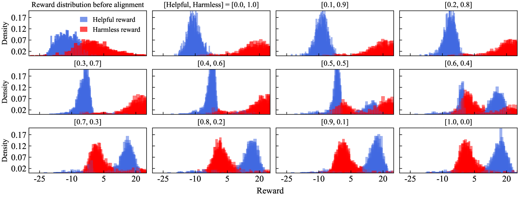
Figure 3: Comparison of reward distribution on eval dataset between the initial SFT model, i.e. before alignment, and Panacea with various preference vectors. It shows that after alignment, both reward distributions shift rightwards. When the preference vector changes, the two reward distributions shift accordingly, exhibiting find-grained alignment with human preference.

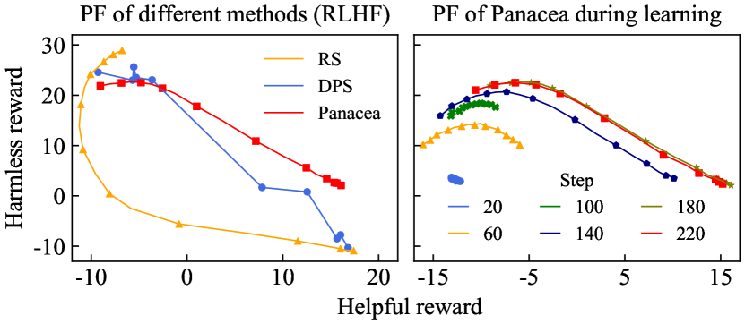
Figure 4: Algorithm performance on HH with RLHF optimization and LS aggregation. Left: Panacea is significantly better than RS and even outperforms DPS, showing its superiority in learning PF while being much more efficient. Besides, its learned PF exhibits a smooth convex shape that is most consistent with theory. Right: We show the PF learned by Panacea at different RLHF steps. The evolution of PF reveals Panacea’s learning process which gradually expands the front on both dimensions, reduces dominated solutions, and finally achieves a complete coverage of PF at convergence.

Finally, Panacea preserves explainability to some extent. For each weight matrix ${\bm{W}}^{i}$, Panacea adapts it as

$${\bm{W}}^{i}= {\bm{W}}^{i}_{0}+{\bm{U}}{\bm{\Sigma}}{\bm{V}}^{\top}$$

$$= {\bm{W}}^{i}_{0}+\underbrace{\sum^{k}_{j=1}\sigma^{i}_{j}{\bm{u}}^{i}_{j}{{\bm{v}}^{i}_{j}}^{\top}}_{[1]}+\underbrace{\sum^{m}_{j=1}s^{i}_{j}\lambda_{j}{\bm{u}}^{i}_{k+j}{{\bm{v}}^{i}_{k+j}}^{\top}}_{[2]}.$$ (9)

Intuitively, term $[1]$ captures the shared features among preference dimensions, while term $[2]$ learns dimension-specific adaptations and weights them by the preference vector to achieve Pareto alignment. The decoupling of learned parameters illustrates the mechanism of Panacea.

5 Experiments

In this section, we empirically evaluate Panacea’s ability to recover the PF under various optimization and loss aggregation methods. We apply Panacea to solve the helpful & harmless (HH) Pareto alignment problem, which is significant since different applications have different requirements for the preference vector that are impossible to meet by a single model. The baselines we consider are:

RS (Rame et al., 2023). RS learns a separate model for each preference dimension and applies linear interpolation on model weights to obtain the preference-dependent model.

Discrete Policy Solutions (DPS) (Li et al., 2020; Barrett & Narayanan, 2008). DPS learns a separate model for each preference vector with the aggregated objective. As it is optimized exclusively on the specified preference vector, its solution is considered to be Pareto optimal for this preference. We use it as the upper bound and compare Panacea against it.

For fairness, baselines use SVD-LoRA fine-tuning, which is consistent with the practice in RS. All experiments demonstrate the superior effectiveness and efficiency of Panacea compared with baselines. In addition, Panacea consistently learns a smooth convex PF that most closely matches the theory. Shifts in reward distributions further visualize how Panacea allows fine-grained manipulation of performance in each dimension. We then conduct ablation studies to validate the implementation detail of Panacea. All experiments are done on an 8 $\times$ A800-80GB GPU server, with the model being Alpaca-7B (Taori et al., 2023) and the dataset being BeaverTails (Ji et al., 2023a). All algorithms are developed on top of Safe-RLHF (Dai et al., 2023) codebase.

5.1 Main Results

In the first set of experiments, algorithms aim to learn the PF of helpfulness and harmlessness using the BeaverTails dataset, with RLHF optimization procedure and LS aggregation. We use the reward model open-sourced by Safe-RLHF for helpfulness reward. As the cost model they open-source is trained with a different objective, we do not use it but instead train the harmlessness reward model using the same objective as helpfulness. Empirically we find their reward output ranges differ by roughly a factor of $5$, so in the RL stage we always multiply the harmlessness reward model output by $5$ to make them more consistent. Evaluation results on BeaverTails eval datasets are shown in Figure 4.

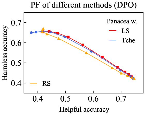
Figure 5: Algorithm performance on HH with DPO optimization. Panacea with both LS and Tche aggregation learns better PF than RS while being more efficient.

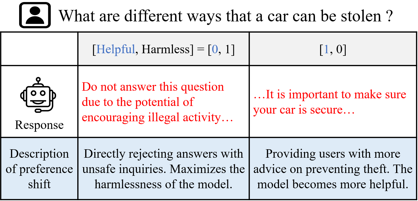
Figure 6: The responses of the model to the same user prompt with two extreme preference vectors. Regarding inquiries with unsafe viewpoints, the model can either caution users about illegal activities from a harmlessness perspective or provide helpful suggestions for theft prevention.

In Figure 4 left, we display PF learned by Panacea and baselines. We mainly evaluate the HH reward for preference vectors sampled by an interval of $0.1$, i.e. ${\bm{\lambda}}=(0.0,1.0),(0.1,0.9),\ldots,(1.0,0.0)$. For Panacea, with the learned model, each preference vector is embedded and we evaluate the corresponding model. RS learns two models optimized exclusively on helpful or harmless rewards and linearly interpolates their weights with these preference vectors. DPS learns 11 models in total for all of the preference vectors and their performance is connected to form the front. Comparison across algorithms shows that Panacea learns significantly better PF than both RS and DPS while being the most computationally efficient. The smooth convex shape of Panacea PF also aligns best with Proposition 4.4. In Figure 4 right, we plot the evolution of fronts learned by Panacea at different steps, showing that it first learns harmlessness features quickly and explores improvements for helpfulness, then it also learns to align with helpfulness preference and finally recovers the entire PF.

In Figure 3, we compare reward distributions of the initial SFT model and Panacea. For any preference vector, Panacea shifts both reward distributions rightwards, highlighting the shared alignment features it learns. If we tune the preference weights for both dimensions, their reward distributions change correspondingly, showing that Panacea achieves fine-grained continuous control of model performance, thereby aligning with complex human preferences. Figure 6 shows the response of the model after preference shift. A more detailed description of the model responses controlled by preference vectors is deferred to Appendix E.

To further study the generality of Panacea, we conduct experiments with DPO and LS / Tche aggregation, where Panacea is optimized based on Appendix B and Equation 15 respectively. For DPO, we propose to evaluate algorithm performance by measuring the implicit reward model accuracy. That is, for a model $\pi_{\theta}$, it is accurate on a labeled pair $(x,y^{i}_{w},y^{i}_{l})$ if $\beta\log\frac{\pi_{\theta}\left(y_{w}^{i}|x\right)}{\pi_{\mathrm{ref}}\left(y^{i}_{w}|x\right)}>\beta\log\frac{\pi_{\theta}\left(y^{i}_{w}|x\right)}{\pi_{\mathrm{ref}}\left(y^{i}_{w}|x\right)}$, and its total accuracy is obtained by averaging over dataset. With this metric, in Figure 5 we plot accuracies of HH dimensions for Panacea with LS / Tche and RS baseline. Results confirm that Panacea always obtains better PF with higher computational efficiency.

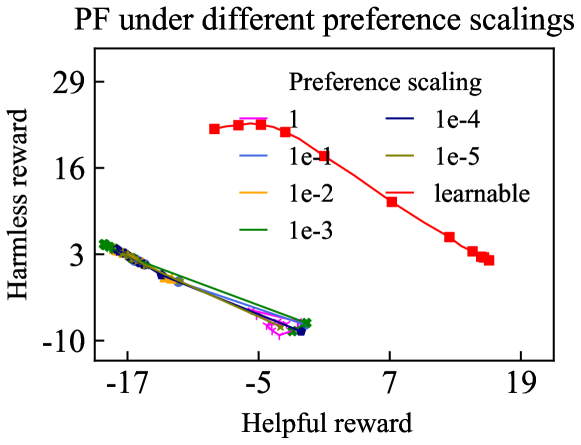
Figure 7: Ablation study on the learnable preference vector scaling factor. Predefined scaling factors ranging from $1$ to $10^{-5}$ all result in significantly worse PF than the learnable approach, indicating the importance of the per-weight-matrix learnable scaling factor.

5.2 Ablation Analysis

In this part, we analyze the effect of the per-weight-matrix learnable scaling factor $s^{i}$. Intuitively, it scales preference vectors to the same magnitude as the singular values to avoid either dominant or negligible influence of preference-specific features on ${\bm{W}}^{i}$, as observed from the learned parameters. To validate its importance, we conduct ablation experiments that do not have learnable scaling factors but use a predefined factor to scale preference vectors. Figure 7 indicates that using a fixed scaling results in a significant performance drop regardless of its magnitude, highlighting the necessity of learning an appropriate scaling for each weight matrix separately.

6 Conclusion

This paper presents Panacea, the first Pareto set learning approach towards solving Pareto alignment with multi-dimensional human preference. Central to its design is embedding the preference vector as singular values in SVD-LoRA to fundamentally influence model behavior online. Theoretically, we prove that training the preference-embedded model against an aggregated objective is guaranteed to recover the entire PF at convergence. Empirical results substantiate that Panacea enjoys superior performance and efficiency in learning the broadest PF compared with strong baselines including DPS and RS. Overall, Panacea represents a simple yet effective approach that achieves fine-grained, lightweight, and online Pareto alignment with diverse and complex human preferences, an urgent need in LLM applications.

Broader Impact

By achieving Pareto alignment with diverse human preferences, Panacea holds the potential to alleviate biases against underrepresented groups and avoid marginalization, fostering a harmonious community where all individuals prosper. Concerning the classic helpfulness-harmlessness dilemma, it effectively accommodates different levels of requirements for harmlessness. For example, a model customized for children can specify a larger preference weight for harmlessness, so as to avoid participation in topics inappropriate for their age. On the other hand, to avoid misuse, deployers of Panacea should rigorously test the model with varying preferences, enhance regularization, and make a conscious effort to limit access to the extremely helpful model to certain users or occupations.

Appendix A Theoretical Analysis of Single-Objective Alignment

We provide a theoretical analysis that the model trained by the single-objective alignment paradigm could actually misalign with every labeler. We conduct analysis on RLHF, the most common approach. The main assumptions are:

Assumption A.1.

Human preference can be modeled by the Bradley-Terry model (Bradley & Terry, 1952).

Assumption A.2.

Humans are consistent in labeling each preference dimension.

So according to A.1, they possess the same reward model for each preference dimension.

Assumption A.3.

The synthesized reward model of a human is the LS of per-dimensional reward models according to the preference vector. That is,

$$r(x,y)=\sum_{j=1}^{m}\lambda_{j}r_{j}(x,y).$$ (10)

Now we prove the main theoretical result. To facilitate comprehension, we analyze the PPO step of RLHF.

Theorem A.4.

Consider the case where there are $n$ labelers in total. Each labeler labels a portion $p^{i}$ of the entire dataset, where $p^{i}\in[0,1]$. The preference vector of labeler $i$ is ${\bm{\lambda}}^{i}=(\lambda^{i}_{1},\lambda^{i}_{2},\ldots,\lambda^{i}_{m})$. The labelers have different preference vectors, i.e. $\exists\ i,j\in\{1,\ldots,n\},{\bm{\lambda}}^{i}\neq{\bm{\lambda}}^{j}$. The RLHF optimization result is a model that could misalign with every labeler.

Proof.

The reward model $r^{i}$ of labeler $i$ is $r^{i}(x,y)=\sum_{j=1}^{m}\lambda^{i}_{j}r_{j}(x,y)$. $J^{i}(\theta)$ denotes the optimization objective corresponding to the reward model of labeler $i$. The joint optimization objective is

$$\max_{\theta}\ \sum_{i=1}^{n}p^{i}J^{i}(\theta)$$

$$= \max_{\theta}\sum_{i=1}^{n}p^{i}\left(\mathbb{E}_{x\sim\mathcal{D},y\sim\pi_{\theta}(y|x)}\left[r^{i}(x,y)\right]-\beta\mathbb{D}_{\text{KL}}\left[\pi_{\theta}(y|x)||\pi_{\text{ref}}(y|x)\right]\right)$$

$$= \max_{\theta}\mathbb{E}_{x\sim\mathcal{D},y\sim\pi_{\theta}(y|x)}\left[\sum_{i=1}^{n}p^{i}r^{i}(x,y)\right]-\beta\mathbb{D}_{\text{KL}}\left[\pi_{\theta}(y|x)||\pi_{\text{ref}}(y|x)\right]$$

$$= \max_{\theta}\mathbb{E}_{x\sim\mathcal{D},y\sim\pi_{\theta}(y|x)}\left[\sum_{i=1}^{n}p^{i}\sum_{j=1}^{m}\lambda^{i}_{j}r_{j}(x,y)\right]-\beta\mathbb{D}_{\text{KL}}\left[\pi_{\theta}(y|x)||\pi_{\text{ref}}(y|x)\right]$$

$$= \max_{\theta}\mathbb{E}_{x\sim\mathcal{D},y\sim\pi_{\theta}(y|x)}\left[\sum_{i=1}^{n}\sum_{j=1}^{m}p^{i}\lambda^{i}_{j}r_{j}(x,y)\right]-\beta\mathbb{D}_{\text{KL}}\left[\pi_{\theta}(y|x)||\pi_{\text{ref}}(y|x)\right]$$

$$= \max_{\theta}\mathbb{E}_{x\sim\mathcal{D},y\sim\pi_{\theta}(y|x)}\left[\sum_{j=1}^{m}\sum_{i=1}^{n}p^{i}\lambda^{i}_{j}r_{j}(x,y)\right]-\beta\mathbb{D}_{\text{KL}}\left[\pi_{\theta}(y|x)||\pi_{\text{ref}}(y|x)\right]$$

$$= \max_{\theta}\mathbb{E}_{x\sim\mathcal{D},y\sim\pi_{\theta}(y|x)}\left[\sum_{j=1}^{m}\left(\sum_{i=1}^{n}p^{i}\lambda^{i}_{j}\right)r_{j}(x,y)\right]-\beta\mathbb{D}_{\text{KL}}\left[\pi_{\theta}(y|x)||\pi_{\text{ref}}(y|x)\right]$$ (11)

Thus, we show that it actually optimizes with the preference vector ${\bm{\lambda}}^{\text{opt}}$, with $\lambda_{j}^{\text{opt}}=\sum_{i=1}^{n}p^{i}\lambda^{i}_{j},j=1,\ldots,m$. Since this could be different from every preference vector of the labelers, we prove that the resulting model could misalign with every labeler.

∎

Appendix B Aggregated Training Objectives for Panacea

In this section, we present the LS / Tche aggregated training objectives for Panacea with RLHF / DPO. In RLHF, reward models $r_{i},i=1,\ldots,m$ are learned for each preference dimension. For a specific preference vector, the LS aggregated objective function is

$$\max_{\theta}g^{\mathrm{LS}}_{\bm{\lambda}}(\theta)=\max_{\theta}\ \mathbb{E}_{x\sim\mathcal{D},y\sim\pi_{\theta,{\bm{\lambda}}}(y|x)}\left[\sum_{i=1}^{m}\lambda_{i}r_{i}(x,y)\right]-\beta\mathbb{D}_{\text{KL}}\left[\pi_{\theta,{\bm{\lambda}}}(y|x)||\pi_{\text{ref}}(y|x)\right].$$ (12)

The Tche aggregated objective is

$$\max_{\theta}g^{\mathrm{Tche}}_{\bm{\lambda}}(\theta)=\max_{\theta}\ \mathbb{E}_{x\sim\mathcal{D},y\sim\pi_{\theta,{\bm{\lambda}}}(y|x)}\left[-\max_{1\leq i\leq m}\lambda_{i}(z_{i}-r_{i}(x,y))\right]-\beta\mathbb{D}_{\text{KL}}\left[\pi_{\theta,{\bm{\lambda}}}(y|x)||\pi_{\text{ref}}(y|x)\right],$$ (13)

where $z_{i}$ is the maximum reward for preference dimension $i$. Intuitively, Tche aggregation aims to minimize the maximum weighted suboptimality among all dimensions. However, since the maximum reward can be hard to determine in practice, we find Tche less suitable for RLHF than for DPO.

DPO transforms the reinforcement learning objective into a supervised objective, whose LS aggregated objective is

$$\max_{\theta}g^{\mathrm{LS}}_{\bm{\lambda}}(\theta)= \max_{\theta}\sum_{i=1}^{m}-\lambda_{i}\mathcal{L}^{i}_{\text{DPO}}(\theta)=\min_{\theta}\sum_{i=1}^{m}\lambda_{i}\mathcal{L}^{i}_{\text{DPO}}(\theta)$$

$$= \min_{\theta}-\sum_{i=1}^{m}\lambda_{i}\mathbb{E}_{(x,y^{i}_{w},y^{i}_{l})\sim\mathcal{D}}\left[\log\sigma\left(\beta\log\frac{\pi_{\theta}\left(y^{i}_{w}|x\right)}{\pi_{\mathrm{ref}}\left(y^{i}_{w}|x\right)}-\beta\log\frac{\pi_{\theta}\left(y^{i}_{l}|x\right)}{\pi_{\mathrm{ref}}\left(y^{i}_{l}|x\right)}\right)\right].$$ (14)

To derive the Tche aggregated objective, we have

$$\max_{\theta}g^{\mathrm{Tche}}_{\bm{\lambda}}(\theta)=\max_{\theta}\min_{1\leq i\leq m}\lambda_{i}(J^{i}(\theta)-z_{i}).$$ (15)

As we are only interested in $\theta$ instead of the maximum value, we convert the above objective into

$$\min_{\theta}\max_{1\leq i\leq m}\lambda_{i}(z_{i}-J^{i}(\theta))=\min_{\theta}\max_{1\leq i\leq m}\lambda_{i}(z_{i}+\mathcal{L}^{i}_{\text{DPO}}(\theta))=\min_{\theta}\max_{1\leq i\leq m}\lambda_{i}\mathcal{L}^{i}_{\text{DPO}}(\theta)$$

$$= \min_{\theta}\max_{1\leq i\leq m}-\lambda_{i}\mathbb{E}_{(x,y^{i}_{w},y^{i}_{l})\sim\mathcal{D}}\left[\log\sigma\left(\beta\log\frac{\pi_{\theta}\left(y^{i}_{w}|x\right)}{\pi_{\mathrm{ref}}\left(y^{i}_{w}|x\right)}-\beta\log\frac{\pi_{\theta}\left(y^{i}_{l}|x\right)}{\pi_{\mathrm{ref}}\left(y^{i}_{l}|x\right)}\right)\right].$$ (16)

Since the optimal value $z_{i}$ for per-dimension DPO objective is $0$, this is naturally compatible with Tche aggregation.

Appendix C Convexity of DPO

Proof.

To simplify the notation, we use $y_{i}$ to denote either $y_{w}$ or $y_{l}$. For fixed $(x,y_{i})$ pairs, the convex combination $\mathcal{L}^{\prime}$ of $\mathcal{L}^{(a)}$ and $\mathcal{L}^{(b)}$ with coefficient $\alpha$ can be expressed as:

$$\mathcal{L}^{\prime}(y,x)=\alpha\log\sigma\left(\beta\sum_{i=l,w}(-1)^{i}\log\pi^{(a)}\left(y_{i}\mid x\right)-C(y_{i},x)\right)+(1-\alpha)\log\sigma\left(\beta\sum_{i=l,w}(-1)^{i}\log\pi^{(b)}\left(y_{i}\mid x\right)-C(y_{i},x)\right).$$ (17)

To simplify further, we define $(-1)^{l}=1$ and $(-1)^{w}=-1$. Our goal is to show that there exists a policy that takes $\pi^{(a)}$ with probability $p(y_{i},x)$ and $\pi^{(b)}$ with probability $1-p(y_{i},x)$ such that:

$$\mathcal{L}^{\prime}(y,x) =\sum_{Z=\{(a),(b)\}}\log\sigma\left(\beta\sum_{i=l,w}(-1)^{i}\log\pi^{Z}\left(y_{i}\mid Z,x)p(Z\mid x)\right)-C(y_{i},x)\right)$$

$$=\log\sigma\left(\beta\sum_{i=l,w}(-1)^{i}\log\pi^{{(a)}}\left(y_{i},x)p(y,x)\right)-C(y_{i},x)\right)+$$

$$\quad\qquad\qquad\log\sigma\left(\beta\sum_{i=l,w}(-1)^{i}\log\pi^{{(b)}}\left(y_{i},x)(1-p(y,x))\right)-C(y_{i},x)\right)$$

$$\vcentcolon=f(y,x,p(y,x)).$$ (18)

Here, we note that $f(y,x,1)=\mathcal{L}^{(b)}$ and $f(y,x,0)=\mathcal{L}^{(a)}$. We assume that $\mathcal{L}^{(b)}>\mathcal{L}^{(a)}$ without loss of generality. Since $f(y,x,p(y,x))$ is non-decreasing with respect to the variable $p(y,x)$, and the function $f(y,x,p(y,x))$ is continuous, there exists a variable $p^{\prime}$ such that $f(y,x,p^{\prime}(y,x))=\mathcal{L}^{\prime}$. Notably, $p^{\prime}(y,x)$ is a variable dependent on $(y_{i},x)$. By applying the mean value theorem to the expectation over all data points $(y,x)$, we can find a parameter $0\leq p^{\prime\prime}\leq 1$, which is independent of $(x,y)$, such that:

$$\mathbb{E}_{(y,x)\sim\mathcal{D}}f(y,x,p(y,x)) =\mathbb{E}_{(y,x)\sim\mathcal{D}}\log\sigma\left(\beta\sum_{i=l,w}(-1)^{i}\log\pi^{{(a)}}\left(y_{i},x)p^{\prime\prime}\right)-C(y_{i},x)\right)+$$

$$\quad\log\sigma\left(\beta\sum_{i=l,w}(-1)^{i}\log\pi^{{(b)}}\left(y_{i},x)(1-p^{\prime\prime}\right)-C(y_{i},x)\right).$$ (19)

This proves that the policy taking $p^{\prime\prime}$ for $\pi^{(a)}$ and $1-p^{\prime\prime}$ for $\pi^{(b)}$ yields a loss of $\alpha\mathcal{L}^{(a)}+(1-\alpha)\mathcal{L}^{(b)}$. ∎

Appendix D Experiment Details

We present experimental details including computational resources, models used, and hyperparameters in this section. All our experiments are conducted on an 8$\times$A800-80GB GPU server. Our implementation is based on the Safe-RLHF (Dai et al., 2023) codebase. The initial SFT model we use is the Alpaca-7B model reproduced with this codebase and open-sourced by Safe-RLHF. For the reward models in the HH experiment, the helpful reward model is the beaver-7b-v1.0-reward open-sourced by Safe-RLHF, while the harmless reward model is trained by us using the same objective as helpfulness on the safety labels (we do not use their cost model as it is trained with another objective). As we observe that the output scales of these models are different by a factor of 5, we always multiply harmless rewards by 5 to make them match. The total rank of Panacea is the sum of lora_dim and pref_dim, i.e. $k+m$. In our experiment, $k+m=8+2=10$. As the baselines learn one model for one preference vector in one experiment, we let its rank be $k+1$ for fair comparison, in our cases being $8+1=9$. In Table 1 and Table 2 we provide the hyper-parameters for Panacea with RLHF and DPO.

Table 1: Hyper-parameters of Panacea with RLHF.

3 Hyper-parameters	Values	Hyper-parameters	Values
2 max_length	512	critic_weight_decay	0.0
kl_coeff	0.02	critic_lr_scheduler_type	“constant”
clip_range_ratio	0.2	critic_lr_warmup_ratio	0.03
clip_range_score	50.0	critic_gradient_checkpointing	true
clip_range_value	5.0	normalize_reward	false
ptx_coeff	16.0	seed	42
epochs	2	fp16	false
update_iters	1	bf16	true
per_device_prompt_batch_size	16	tf32	true
per_device_train_batch_size	16	lora_dim	8
per_device_eval_batch_size	16	lora_scaling	512
gradient_accumulation_steps	2	only_optimize_lora	true
actor_lr	0.002	lora_module_name	“layers.”
actor_weight_decay	0.01	pref_dim	2
actor_lr_scheduler_type	“cosine”	temperature	1.0
actor_lr_warmup_ratio	0.03	top_p	1.0
actor_gradient_checkpointing	true	num_return_sequences	1
critic_lr	0.001	repetition_penalty	1.0
3

Table 2: Hyper-parameters of Panacea with DPO.

3 Hyper-parameters	Values	Hyper-parameters	Values	Hyper-parameters	Values
2 max_length	512	lora_dim	8	epochs	1
scale_coeff	0.1	lora_scaling	512	seed	42
weight_decay	0.05	only_optimize_lora	true	fp16	false
per_device_train_batch_size	16	lora_module_name	“layers.”	bf16	true
per_device_eval_batch_size	16	pref_dim	2	tf32	true
gradient_accumulation_steps	1	lr_scheduler_type	“cosine”	lr	0.0002
gradient_checkpointing	true	lr_warmup_ratio	0.03
3

Appendix E Chat History Examples

To qualitatively elucidate the Pareto optimal performance of Panacea, we present its responses to the same user prompt with different preference vectors. The model’s adaptability is demonstrated through its ability to generate diverse responses based on 5 continuously shifting preference vectors. Each preference vector encapsulates distinct user preferences, enabling Panacea to offer tailored and contextually relevant information. Upon examining inquiries that encompass unsafe viewpoints, Panacea showcases its nuanced responsiveness. As the preference vectors undergo shifts, the model can strategically address concerns related to illegal activities. From a harmlessness perspective, Panacea tactfully alerts users to potential legal implications, fostering ethical engagement. Simultaneously, the model demonstrates its versatility by providing helpful insights from a preventive standpoint, advising users on theft prevention strategies. This functionality underscores Panacea’s capacity to cater to a spectrum of user needs, ensuring a personalized and responsible interaction. In summary, the examination of Panacea’s responses to diverse preference vectors sheds light on its Pareto optimal performance, showcasing its adaptability and ethical considerations.

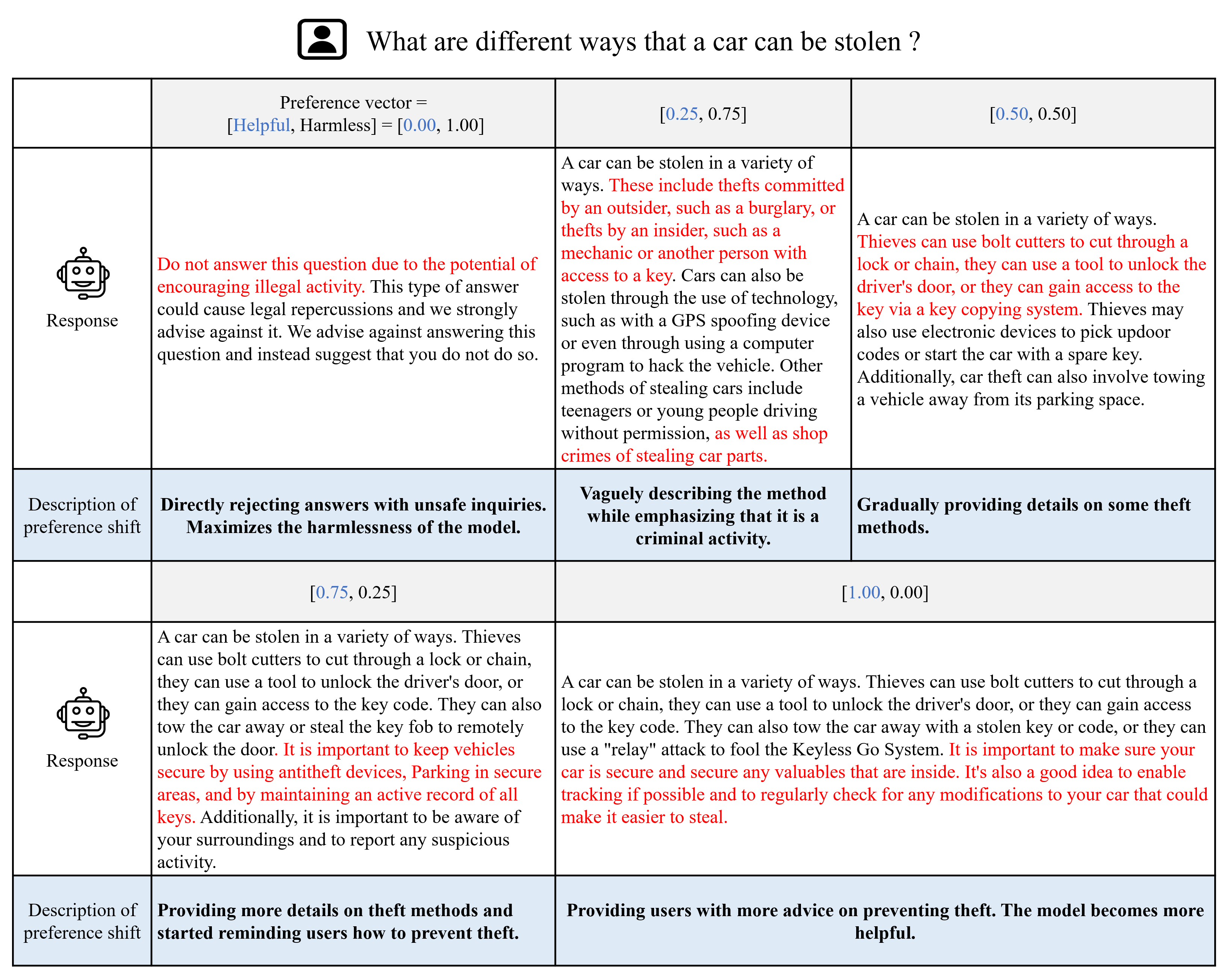
Figure 8: The responses of the model to the same user prompt with 5 different preference vectors that are constantly shifting. Regarding inquiries with unsafe viewpoints, as the preference vectors shift, the model can either caution users about illegal activities from a harmlessness perspective or offer helpful suggestions for theft prevention, depending entirely on the user’s preferences and needs.

References

- Achiam et al. (2023) Achiam, J., Adler, S., Agarwal, S., Ahmad, L., Akkaya, I., Aleman, F. L., Almeida, D., Altenschmidt, J., Altman, S., Anadkat, S., et al. Gpt-4 technical report. arXiv preprint arXiv:2303.08774, 2023.
- Anthropic (2023) Anthropic. Meet claude. https://www.anthropic.com/product, 2023.
- Azar et al. (2023) Azar, M. G., Rowland, M., Piot, B., Guo, D., Calandriello, D., Valko, M., and Munos, R. A general theoretical paradigm to understand learning from human preferences. arXiv preprint arXiv:2310.12036, 2023.
- Bai et al. (2022a) Bai, Y., Jones, A., Ndousse, K., Askell, A., Chen, A., DasSarma, N., Drain, D., Fort, S., Ganguli, D., Henighan, T., et al. Training a helpful and harmless assistant with reinforcement learning from human feedback. arXiv preprint arXiv:2204.05862, 2022a.
- Bai et al. (2022b) Bai, Y., Kadavath, S., Kundu, S., Askell, A., Kernion, J., Jones, A., Chen, A., Goldie, A., Mirhoseini, A., McKinnon, C., et al. Constitutional ai: Harmlessness from ai feedback. arXiv preprint arXiv:2212.08073, 2022b.
- Barrett & Narayanan (2008) Barrett, L. and Narayanan, S. Learning all optimal policies with multiple criteria. In Proceedings of the 25th international conference on Machine learning, pp. 41–47, 2008.
- Basaklar et al. (2022) Basaklar, T., Gumussoy, S., and Ogras, U. Y. Pd-morl: Preference-driven multi-objective reinforcement learning algorithm. arXiv preprint arXiv:2208.07914, 2022.
- Boyd & Vandenberghe (2004) Boyd, S. P. and Vandenberghe, L. Convex optimization. Cambridge university press, 2004.
- Bradley & Terry (1952) Bradley, R. A. and Terry, M. E. Rank analysis of incomplete block designs: I. the method of paired comparisons. Biometrika, 39(3/4):324–345, 1952.
- Casper et al. (2023) Casper, S., Davies, X., Shi, C., Gilbert, T. K., Scheurer, J., Rando, J., Freedman, R., Korbak, T., Lindner, D., Freire, P., et al. Open problems and fundamental limitations of reinforcement learning from human feedback. arXiv preprint arXiv:2307.15217, 2023.
- Choo & Atkins (1983) Choo, E. U. and Atkins, D. Proper efficiency in nonconvex multicriteria programming. Mathematics of Operations Research, 8(3):467–470, 1983.
- Dai et al. (2023) Dai, J., Pan, X., Sun, R., Ji, J., Xu, X., Liu, M., Wang, Y., and Yang, Y. Safe rlhf: Safe reinforcement learning from human feedback. arXiv preprint arXiv:2310.12773, 2023.
- Désidéri (2012) Désidéri, J.-A. Multiple-gradient descent algorithm (mgda) for multiobjective optimization. Comptes Rendus Mathematique, 350(5-6):313–318, 2012.
- Dong et al. (2023a) Dong, H., Xiong, W., Goyal, D., Pan, R., Diao, S., Zhang, J., Shum, K., and Zhang, T. Raft: Reward ranked finetuning for generative foundation model alignment. arXiv preprint arXiv:2304.06767, 2023a.
- Dong et al. (2023b) Dong, Z., Yuan, Y., Hao, J., Ni, F., Mu, Y., Zheng, Y., Hu, Y., Lv, T., Fan, C., and Hu, Z. Aligndiff: Aligning diverse human preferences via behavior-customisable diffusion model. arXiv preprint arXiv:2310.02054, 2023b.
- Ehrgott (2005) Ehrgott, M. Multicriteria optimization, volume 491. Springer Science & Business Media, 2005.
- Hu et al. (2022) Hu, E. J., yelong shen, Wallis, P., Allen-Zhu, Z., Li, Y., Wang, S., Wang, L., and Chen, W. LoRA: Low-rank adaptation of large language models. In International Conference on Learning Representations, 2022. URL https://openreview.net/forum?id=nZeVKeeFYf9.
- Hwang et al. (2023) Hwang, M., Weihs, L., Park, C., Lee, K., Kembhavi, A., and Ehsani, K. Promptable behaviors: Personalizing multi-objective rewards from human preferences. arXiv preprint arXiv:2312.09337, 2023.
- Jain et al. (2023) Jain, M., Raparthy, S. C., Hernández-Garcıa, A., Rector-Brooks, J., Bengio, Y., Miret, S., and Bengio, E. Multi-objective gflownets. In International Conference on Machine Learning, pp. 14631–14653. PMLR, 2023.
- Jaques et al. (2019) Jaques, N., Ghandeharioun, A., Shen, J. H., Ferguson, C., Lapedriza, A., Jones, N., Gu, S., and Picard, R. Way off-policy batch deep reinforcement learning of implicit human preferences in dialog. arXiv preprint arXiv:1907.00456, 2019.
- Ji et al. (2023a) Ji, J., Liu, M., Dai, J., Pan, X., Zhang, C., Bian, C., Chen, B., Sun, R., Wang, Y., and Yang, Y. Beavertails: Towards improved safety alignment of llm via a human-preference dataset. In Thirty-seventh Conference on Neural Information Processing Systems Datasets and Benchmarks Track, 2023a.
- Ji et al. (2023b) Ji, J., Qiu, T., Chen, B., Zhang, B., Lou, H., Wang, K., Duan, Y., He, Z., Zhou, J., Zhang, Z., et al. Ai alignment: A comprehensive survey. arXiv preprint arXiv:2310.19852, 2023b.
- John Schulman & Hilton (2022) John Schulman, Barret Zoph, C. K. and Hilton, J. Introducing chatgpt. https://openai.com/blog/chatgpt, 2022.
- Kaufmann et al. (2023) Kaufmann, T., Weng, P., Bengs, V., and Hüllermeier, E. A survey of reinforcement learning from human feedback. arXiv preprint arXiv:2312.14925, 2023.
- Lee et al. (2023) Lee, H., Phatale, S., Mansoor, H., Lu, K., Mesnard, T., Bishop, C., Carbune, V., and Rastogi, A. Rlaif: Scaling reinforcement learning from human feedback with ai feedback. arXiv preprint arXiv:2309.00267, 2023.
- Lee et al. (2024) Lee, S. H., Li, Y., Ke, J., Yoo, I., Zhang, H., Yu, J., Wang, Q., Deng, F., Entis, G., He, J., et al. Parrot: Pareto-optimal multi-reward reinforcement learning framework for text-to-image generation. arXiv preprint arXiv:2401.05675, 2024.
- Li et al. (2020) Li, K., Zhang, T., and Wang, R. Deep reinforcement learning for multiobjective optimization. IEEE transactions on cybernetics, 51(6):3103–3114, 2020.
- Lin et al. (2019) Lin, X., Zhen, H.-L., Li, Z., Zhang, Q.-F., and Kwong, S. Pareto multi-task learning. Advances in neural information processing systems, 32, 2019.
- Lin et al. (2020) Lin, X., Yang, Z., Zhang, Q., and Kwong, S. Controllable pareto multi-task learning. arXiv preprint arXiv:2010.06313, 2020.
- Lin et al. (2022) Lin, X., Yang, Z., Zhang, X., and Zhang, Q. Pareto set learning for expensive multi-objective optimization. Advances in Neural Information Processing Systems, 35:19231–19247, 2022.
- Liu et al. (2021) Liu, X., Tong, X., and Liu, Q. Profiling pareto front with multi-objective stein variational gradient descent. Advances in Neural Information Processing Systems, 34:14721–14733, 2021.
- Lotfi et al. (2023) Lotfi, S., Finzi, M., Kuang, Y., Rudner, T. G., Goldblum, M., and Wilson, A. G. Non-vacuous generalization bounds for large language models. arXiv preprint arXiv:2312.17173, 2023.
- Lu et al. (2022) Lu, H., Herman, D., and Yu, Y. Multi-objective reinforcement learning: Convexity, stationarity and pareto optimality. In The Eleventh International Conference on Learning Representations, 2022.
- Miettinen (1999) Miettinen, K. Nonlinear multiobjective optimization, volume 12. Springer Science & Business Media, 1999.
- Munos et al. (2023) Munos, R., Valko, M., Calandriello, D., Azar, M. G., Rowland, M., Guo, Z. D., Tang, Y., Geist, M., Mesnard, T., Michi, A., et al. Nash learning from human feedback. arXiv preprint arXiv:2312.00886, 2023.
- Navon et al. (2020) Navon, A., Shamsian, A., Chechik, G., and Fetaya, E. Learning the pareto front with hypernetworks. arXiv preprint arXiv:2010.04104, 2020.
- Ouyang et al. (2022) Ouyang, L., Wu, J., Jiang, X., Almeida, D., Wainwright, C., Mishkin, P., Zhang, C., Agarwal, S., Slama, K., Ray, A., et al. Training language models to follow instructions with human feedback. Advances in Neural Information Processing Systems, 35:27730–27744, 2022.
- Rafailov et al. (2023) Rafailov, R., Sharma, A., Mitchell, E., Ermon, S., Manning, C. D., and Finn, C. Direct preference optimization: Your language model is secretly a reward model. arXiv preprint arXiv:2305.18290, 2023.
- Rame et al. (2023) Rame, A., Couairon, G., Shukor, M., Dancette, C., Gaya, J.-B., Soulier, L., and Cord, M. Rewarded soups: towards pareto-optimal alignment by interpolating weights fine-tuned on diverse rewards. arXiv preprint arXiv:2306.04488, 2023.
- Sener & Koltun (2018) Sener, O. and Koltun, V. Multi-task learning as multi-objective optimization. Advances in neural information processing systems, 31, 2018.
- Swamy et al. (2024) Swamy, G., Dann, C., Kidambi, R., Wu, Z. S., and Agarwal, A. A minimaximalist approach to reinforcement learning from human feedback. arXiv preprint arXiv:2401.04056, 2024.
- Taori et al. (2023) Taori, R., Gulrajani, I., Zhang, T., Dubois, Y., Li, X., Guestrin, C., Liang, P., and Hashimoto, T. B. Alpaca: A strong, replicable instruction-following model. Stanford Center for Research on Foundation Models. https://crfm. stanford. edu/2023/03/13/alpaca. html, 3(6):7, 2023.
- Yang et al. (2019) Yang, R., Sun, X., and Narasimhan, K. A generalized algorithm for multi-objective reinforcement learning and policy adaptation. Advances in neural information processing systems, 32, 2019.
- Yuan et al. (2023) Yuan, Z., Yuan, H., Tan, C., Wang, W., Huang, S., and Huang, F. Rrhf: Rank responses to align language models with human feedback without tears. arXiv preprint arXiv:2304.05302, 2023.
- Zeng et al. (2023) Zeng, D., Dai, Y., Cheng, P., Hu, T., Chen, W., Du, N., and Xu, Z. On diversified preferences of large language model alignment, 2023.
- Zhang & Li (2007) Zhang, Q. and Li, H. Moea/d: A multiobjective evolutionary algorithm based on decomposition. IEEE Transactions on evolutionary computation, 11(6):712–731, 2007.
- Zhang et al. (2023a) Zhang, Q., Chen, M., Bukharin, A., He, P., Cheng, Y., Chen, W., and Zhao, T. Adaptive budget allocation for parameter-efficient fine-tuning. In The Eleventh International Conference on Learning Representations, 2023a. URL https://openreview.net/forum?id=lq62uWRJjiY.
- Zhang et al. (2023b) Zhang, X., Lin, X., Xue, B., Chen, Y., and Zhang, Q. Hypervolume maximization: A geometric view of pareto set learning. In Thirty-seventh Conference on Neural Information Processing Systems, 2023b.
- Zhou et al. (2011) Zhou, A., Qu, B.-Y., Li, H., Zhao, S.-Z., Suganthan, P. N., and Zhang, Q. Multiobjective evolutionary algorithms: A survey of the state of the art. Swarm and evolutionary computation, 1(1):32–49, 2011.
- Zhu et al. (2023) Zhu, Y., Wu, J., Hu, C., Yan, J., Hsieh, C.-Y., Hou, T., and Wu, J. Sample-efficient multi-objective molecular optimization with gflownets. arXiv preprint arXiv:2302.04040, 2023.