Riemannian Bilevel Optimization

Abstract

In this work, we consider the bilevel optimization problem on Riemannian manifolds. We inspect the calculation of the hypergradient of such problems on general manifolds and thus enable the utilization of gradient-based algorithms to solve such problems. The calculation of the hypergradient requires utilizing the notion of Riemannian cross-derivative and we inspect the properties and the numerical calculations of Riemannian cross-derivatives. Algorithms in both deterministic and stochastic settings, named respectively RieBO and RieSBO, are proposed that include the existing Euclidean bilevel optimization algorithms as special cases. Numerical experiments on robust optimization on Riemannian manifolds are presented to show the applicability and efficiency of the proposed methods.

1 Introduction

Bilevel optimization has drawn attentions from various fields in optimization and machine learning communities, due to its wide range of applications including meta learning (Rajeswaran et al., 2019; Ji et al., 2020), hyperparameter optimization (Okuno et al., 2021; Yu and Zhu, 2020), reinforcement learning (Konda and Tsitsiklis, 1999; Hong et al., 2020) and signal processing (Kunapuli et al., 2008; Flamary et al., 2014). In this work, we focus on the manifold-constrained bilevel optimization problem, which can be formulated as:

$$\min_{x\in\mathcal{M}}\Phi(x):=f(x,y^{*}(x))$$ (1.1)

$$\text{ s.t. }y^{*}(x)=\mathop{\mathrm{missing}}{argmin}_{y\in\mathcal{N}}g(x,y),$$

where $\mathcal{M}$ and $\mathcal{N}$ are $m$ and $n$-dimensional complete Riemannian manifolds, respectively. We also consider the stochastic bilevel optimization which is in the following form:

$$\min_{x\in\mathcal{M}}\Phi(x)=f\left(x,y^{*}(x)\right):=\mathbb{E}_{\xi}\left[F\left(x,y^{*}(x);\xi\right)\right]$$ (1.2)

$$\text{ s.t. }y^{*}(x)=\underset{y\in\mathcal{N}}{\mathop{\mathrm{missing}}{argmin}}\ g(x,y):=\mathbb{E}_{\zeta}[G(x,y;\zeta)],$$

where $\xi$ and $\zeta$ are random variables that usually represent the randomness from the data. Such a framework allows us to utilize the stochastic gradient methods to get a desired convergence result with only a noisy estimate of the gradients for $f$ and $g$. Here we also assume that $g$ is a (geodesically) strongly convex function with respect to $y$ in both (1.1) and (1.2) so that the solution to the lower level problem $y^{*}(x)$ is well-defined.

Notice that the original (Euclidean) bilevel optimization is a special case of (1.1) by taking the manifolds as the Euclidean spaces with the same dimensions:

$$\min_{x\in\mathbb{R}^{m}}\Phi(x):=f(x,y^{*}(x))$$ (1.3)

$$\text{ s.t. }y^{*}(x)=\mathop{\mathrm{missing}}{argmin}_{y\in\mathbb{R}^{n}}g(x,y),$$

where $f$ and $g$ are assumed to be continuously differentiable. It is worth noticing that the objective function $\Phi(x)$ is still nonconvex even if we impose convexity assumptions on $f$, which makes such a problem hard to tackle, let alone the more complicated manifold-constraint problems, namely (1.1) and (1.2).

There has been an extensive study on the Euclidean bilevel optimization (Ji et al., 2021; Hong et al., 2020; Chen et al., 2021b; Ghadimi and Wang, 2018). On the algorithmic sense, the bilevel optimization seeks to obtain a first-order $\epsilon$-stationary point (Definition 4.1 and 5.1 for deterministic and stochastic cases, respectively) with the access to the gradient oracle of $f$ and $g$, as well as the Jacobian- and Hessian-vector product, i.e. $\nabla_{x}\nabla_{y}g(x,y)v$ and $\nabla_{y}^{2}g(x,y)v$, respectively. To find an $\epsilon$-stationary point, we denote the number of calls to the gradient oracle of $f$ and $g$ as $\operatorname{Gc}(f,\epsilon)$ and $\operatorname{Gc}(g,\epsilon)$, correspondingly; similarly we have the notation $\operatorname{JV}$ and $\operatorname{HV}$ for the number of oracle calls for the Jacobian- and Hessian-vector product. In the Euclidean setting, We have Tables 1 and 2 as the summary for the oracle calls to achieve an $\epsilon$-stationary point for deterministic and stochastic cases, correspondingly (and we denote $\kappa$ as the condition number of the lower level strongly convex problem).

Algorithm	BA	AID-BiO	ITD-BiO*
$y$-update	GD	GD	GD
$\operatorname{Gc}(f,\epsilon)$	$\mathcal{O}(\kappa^{4}\epsilon^{-1})$	$\mathcal{O}(\kappa^{3}\epsilon^{-1})$	$\mathcal{O}(\kappa^{3}\epsilon^{-1})$
$\operatorname{Gc}(g,\epsilon)$	$\mathcal{O}(\kappa^{5}\epsilon^{-5/4})$	$\mathcal{O}(\kappa^{4}\epsilon^{-1})$	$\mathcal{O}(\kappa^{4}\epsilon^{-1})$
$\operatorname{JV}(g,\epsilon)$	$\mathcal{O}(\kappa^{4}\epsilon^{-1})$	$\mathcal{O}(\kappa^{3}\epsilon^{-1})$	$\mathcal{O}(\kappa^{4}\epsilon^{-1})$
$\operatorname{HV}(g,\epsilon)$	$\mathcal{O}(\kappa^{4.5}\epsilon^{-1})$	$\mathcal{O}(\kappa^{3.5}\epsilon^{-1})$	$\mathcal{O}(\kappa^{4}\epsilon^{-1})$

* Require explicit assumption on the sequence.

Table 1: Summary of the convergence results for different algorithms for deterministic Euclidean bilevel optimization, including BA (Ghadimi and Wang, 2018), AID-BiO (Ji et al., 2021) and ITD-BiO (Ji et al., 2021).

Algorithm	BSA	Stoc-BiO	TTSA*	ALSET	STABLE*
batch size	$\mathcal{O}(1)$	$\mathcal{O}(\epsilon^{-1})$	$\mathcal{O}(1)$	$\mathcal{O}(1)$	$\mathcal{O}(1)$
$y$-update	$\mathcal{O}(\epsilon^{-1})$ steps SGD	SGD	SGD	SGD	correction
$\operatorname{Gc}(F,\epsilon)$	$\mathcal{O}(\kappa^{6}\epsilon^{-2})$	$\mathcal{O}(\kappa^{5}\epsilon^{-2})$	$\mathcal{O}(\operatorname{poly}(\kappa)\epsilon^{-2.5})$	$\mathcal{O}(\kappa^{5}\epsilon^{-2})$	$\mathcal{O}(\operatorname{poly}(\kappa)\epsilon^{-2})$
$\operatorname{Gc}(G,\epsilon)$	$\mathcal{O}(\kappa^{9}\epsilon^{-2})$	$\mathcal{O}(\kappa^{9}\epsilon^{-2})$	$\mathcal{O}(\operatorname{poly}(\kappa)\epsilon^{-2.5})$	$\mathcal{O}(\kappa^{9}\epsilon^{-2})$	$\mathcal{O}(\operatorname{poly}(\kappa)\epsilon^{-2})$
$\operatorname{JV}(G,\epsilon)$	$\mathcal{O}(\kappa^{6}\epsilon^{-2})$	$\mathcal{O}(\kappa^{5}\epsilon^{-2})$	$\mathcal{O}(\operatorname{poly}(\kappa)\epsilon^{-2.5})$	$\mathcal{O}(\kappa^{5}\epsilon^{-2})$	$\mathcal{O}(\operatorname{poly}(\kappa)\epsilon^{-2})$
$\operatorname{HV}(G,\epsilon)$	$\mathcal{O}(\kappa^{6}\epsilon^{-2})$	$\mathcal{O}(\kappa^{6}\epsilon^{-2})$	$\mathcal{O}(\operatorname{poly}(\kappa)\epsilon^{-2.5})$	$\mathcal{O}(\kappa^{6}\epsilon^{-2})$	$\mathcal{O}(\operatorname{poly}(\kappa)\epsilon^{-2})$

* For algorithms that did not specify the dependence on condition number $\kappa$, we use the notation $\operatorname{poly}(\kappa)$ to summarize the $\kappa$ dependence.

Table 2: Summary of the convergence results for different algorithms for stochastic Euclidean bilevel optimization, including BSA (Ghadimi and Wang, 2018), Stoc-BiO (Ji et al., 2021), TTSA (Hong et al., 2020), ALSET (Chen et al., 2021b) and STABLE (Chen et al., 2021a). For the batch size we only include the $\epsilon$ dependency.

1.1 Main results

In this work, we first analyze the method of calculating and estimating the hypergradient for bilevel problems on Riemannian manifolds. Our propositions include the Euclidean bilevel problems as special cases and involve the calculation of Riemannian cross derivatives, which are of independent interests to the Riemannian optimization field.

Our contribution also lies in proposing two algorithms (RieBO and RieSBO) for both the problems (1.1) and (1.2) correspondingly. For the deterministic problem (1.1), our analysis shows that with a multi-step inner loop and a single-step outer loop, one could yield the similar gradient complexities $\operatorname{Gc}(f,\epsilon)$, $\operatorname{Gc}(g,\epsilon)$, Jacobian- and Hessian-vector product complexities $\operatorname{JV}(g,\epsilon)$ and $\operatorname{HV}(g,\epsilon)$ same as the Euclidean counterparts in Ji et al. (2021), as presented in Table 3, al well as for the stochastic problem (1.2) (Chen et al., 2021b). It is worth noticing that for the stochastic problem, we adopt the framework of Chen et al. (2021b) onto Riemannian manifolds so that the batch-size of the hypergradient estimate can be $\mathcal{O}(1)$, significantly smaller than $\mathcal{O}(\epsilon^{-1})$ as in Ji et al. (2021).

Algorithm	RieBO (Algorithm 1)	RieSBO (Algorithm 2)
batch size	No batch	$\mathcal{O}(1)$
$y$-update	GD	SGD
$\operatorname{Gc}(F,\epsilon)$	$\mathcal{O}(\kappa^{3}\epsilon^{-1})$	$\mathcal{O}(\kappa^{5}\epsilon^{-2})$
$\operatorname{Gc}(G,\epsilon)$	$\mathcal{O}(\kappa^{4}\epsilon^{-1})$	$\mathcal{O}(\kappa^{9}\epsilon^{-2})$
$\operatorname{JV}(G,\epsilon)$	$\mathcal{O}(\kappa^{3}\epsilon^{-1})$	$\mathcal{O}(\kappa^{5}\epsilon^{-2})$
$\operatorname{HV}(G,\epsilon)$	$\mathcal{O}(\kappa^{3.5}\epsilon^{-1})$	$\mathcal{O}(\kappa^{6}\epsilon^{-2})$

Table 3: Summary of the convergence results for the proposed algorithms in this paper, where all the oracles are with respect to Riemannian gradients and Riemannian second-order derivatives. RieBO (Algorithm 1) solves (1.1), and RieSBO (Algorithm 2) solves (1.2).

Finally, we implement the proposed method in the manifold-constrained bilevel optimization problems, namely the distributionally robust optimization on Riemannian manifolds with two specific examples: robust maximum likelihood estimation and robust Karcher mean problem on the manifold of positive definite matrices. These numerical results demonstrate the efficiency and potential applicability of the proposed methods.

1.2 Related works

Bilevel optimization. Bilevel optimization problem, also known as nested optimization problem, whose origin dates back to the 50s and 70s (Stackelberg and Peacock, 1952; Bracken and McGill, 1973). Since then, extensive studies have been conducted for solving the bilevel optimization problem (Shi et al., 2005; Moore, 2010). Recently, gradient-based algorithms for solving bilevel optimization problems draw attention because of their applications in machine learning, see, e.g. Domke (2012); Pedregosa (2016); Gould et al. (2016); Maclaurin et al. (2015); Franceschi et al. (2018); Liao et al. (2018); Shaban et al. (2019); Liu et al. (2020); Li et al. (2020); Grazzi et al. (2020); Lorraine et al. (2020); Ji and Liang (2021); Ghadimi and Wang (2018); Hong et al. (2020); Ji et al. (2021); Chen et al. (2021b, a), among which there has been discussions about the rate of convergence for specific algorithms (Ghadimi and Wang, 2018; Hong et al., 2020; Ji et al., 2021; Chen et al., 2021a, b). These well-established convergence rate results are summarized in Tables 1 and 2. Recently, a line of work (Khanduri et al., 2021; Yang et al., 2023) which utilizes the momentum-based stochastic algorithms can achieve a better oracle complexity of $\mathcal{O}(\epsilon^{-1.5})$ for the Euclidean version of the stochastic problem (1.2). We did not include this line of work since the Riemannian counterparts of these works would rely on the utilization of parallel/vector transport in the algorithm updates. We deliberately avoid these complicated operations in algorithm design and postpone them for future works.

It is worth mentioning that minimax saddle point problems $\min_{x}\max_{y}f(x,y)$ are special cases of bilevel optimization problems by taking $g=-f$. Minimax problems are of great interests to the machine learning community (Daskalakis and Panageas, 2018; Mokhtari et al., 2020; Yoon and Ryu, 2021; Lin et al., 2020b). The analysis of this paper relates to the nonconvex-strongly-concave minimax problem on Riemannian manifolds as in Huang et al. (2020), which showed that the Riemannian gradient descent ascent (RGDA) achieves oracle calls with orders $\mathcal{O}(\kappa^{2}\epsilon^{-1})$ for the deterministic case and $\mathcal{O}(\kappa^{3}\epsilon^{-2})$ for the stochastic case. These results match our convergence results in terms of the order of $\epsilon$, but has better $\kappa$ dependence. This makes sense because our proposed method is a multi-$y$ step GDmax algorithm (see (Nouiehed et al., 2019; Jin et al., 2020)) when applied to the minimax problem and naturally has a larger $\kappa$ dependence. Recently, the authors of Cai et al. (2023) considered the minimax game on Riemannian manifolds under the assumption of geodesic-strongly-monotone (a generalization of strongly-convex-strongly-concave minimax game) and provided a stochastic Riemannian gradient descent-ascent approach which enjoys linear rate of convergence – similar to its Euclidean counterpart. We point out that our work considers nonconvex upper level problems, which is different from the setting in Cai et al. (2023).

Other bilevel-related ongoing research topics include decentralized bilevel optimization Chen et al. (2022, 2023b); Dong et al. (2023), federate bilevel optimization Tarzanagh et al. (2022), bilevel without lower strongly convexity Chen et al. (2023a), to name a few.

Optimization on Riemannian manifolds. Optimization on Riemannian manifolds draws lots of attention recently due to its applications in various fields, including low-rank matrix completion (Boumal and Absil, 2011; Vandereycken, 2013), phase retrieval (Bendory et al., 2017; Sun et al., 2018), dictionary learning (Cherian and Sra, 2016; Sun et al., 2016), dimensionality reduction (Harandi et al., 2017; Tripuraneni et al., 2018; Mishra et al., 2019) and manifold regression (Lin et al., 2017, 2020a). The manifold optimization usually transforms an manifold constrained problem into an unconstrained problem by viewing the manifold as the ambient space and using proper retraction to deal with the loss of linearity, thus achieves better convergence results. For smooth Riemannian optimization, it can be shown that Riemannian gradient descent method require $\mathcal{O}(1/{\epsilon})$ iterations to converge to an $\epsilon$-stationary point (i.e. bounding the norm square of the gradient by $\epsilon$) (Boumal et al., 2018). Stochastic algorithms were also studied for smooth Riemannian optimization (Bonnabel, 2013; Zhou et al., 2019; Weber and Sra, 2019; Zhang et al., 2016; Kasai et al., 2018).

The combination of bilevel optimization with Riemannian optimization is largely blank. Bonnel et al. (2015) considered a semi-vectorial bilevel optimization model over Riemannian manifolds, which deals with the situation where the lower level problem does not have unique solutions and necessary optimality conditions are provided for their surrogate model. To the best of our knowledge, there lacks convergence analysis for Riemannian bilevel optimization in the literature.

2 Preliminaries on Riemannian Optimization

In this part, we briefly review the basic tools we use for optimization on Riemannian manifolds (Lee, 2006; Tu, 2011; Boumal, 2023). Suppose $\mathcal{M}$ is an $m$-dimensional differentiable manifold. The tangent space $\operatorname{T}_{x}\mathcal{M}$ at $x\in\mathcal{M}$ is a linear subspace that consists of the derivatives of all differentiable curves on $\mathcal{M}$ passing through $x$: $\operatorname{T}_{x}\mathcal{M}:=\{\gamma^{\prime}(0):\gamma(0)=x,\gamma([-\delta,\delta])\subset\mathcal{M}\text{ for some }\delta>0,\gamma\text{ is differentiable}\}$. Notice that for every vector $\gamma^{\prime}(0)\in\operatorname{T}_{x}\mathcal{M}$, it can be defined in a coordinate-free sense via the operation over smooth functions: $\forall f\in C^{\infty}(\mathcal{M})$, $\gamma^{\prime}(0)(f):=\frac{df\circ\gamma(t)}{dt}\mid_{t=0}$. The notion of Riemannian manifold is defined as follows.

Definition 2.1 (Riemannian manifold).

Manifold $\mathcal{M}$ is a Riemannian manifold if it is equipped with an inner product on the tangent space, $\langle\cdot,\cdot\rangle_{x}:\operatorname{T}_{x}\mathcal{M}\times\operatorname{T}_{x}\mathcal{M}\rightarrow\mathbb{R}$, that varies smoothly on $\mathcal{M}$. The $(0,2)$-tensor field $g$ is usually referred to as Riemannian metric.

We also review the notion of the differential between manifolds here.

Definition 2.2 (Differential and Riemannian gradients).

Let $F:\mathcal{M}\rightarrow\mathcal{N}$ be a $C^{\infty}$ map between two differential manifolds. At each point $x\in\mathcal{M}$, the differential of $F$ is a mapping (also known as the push-forward):

$$\mathrm{D}F:\operatorname{T}_{x}\mathcal{M}\rightarrow\operatorname{T}_{F(x)}\mathcal{N},$$

such that $\forall\xi\in\operatorname{T}_{x}\mathcal{M}$, $\mathrm{D}F(\xi)\in\operatorname{T}_{x}\mathcal{N}$ is given by

$$(\mathrm{D}F(\xi))(f):=\xi(f\circ F)\in\mathbb{R},\ \forall f\in C_{F(x)}^{\infty}(\mathcal{M}).$$

If $\mathcal{N}=\mathbb{R}$, i.e. $f\in C^{\infty}(\mathcal{M})$, the differential of $f$ is usually denoted as $\mathrm{d}f$. For a Riemannian manifold with Riemannian metric $\langle\cdot,\cdot\rangle$, the Riemannian gradient for $f\in C^{\infty}(\mathcal{M})$ is the unique tangent vector $\mathsf{grad}f(x)\in\operatorname{T}_{x}\mathcal{M}$ satisfying

$$\mathrm{d}f(\xi)=\langle\mathsf{grad}f,\xi\rangle_{x},\ \forall\xi\in\operatorname{T}_{x}\mathcal{M}.$$

For the convergence analysis, we also need the notion of exponential mapping and parallel transport. To this end, we need to first recall the definition of a geodesic.

Definition 2.3 (Geodesic and exponential mapping).

Given $x\in\mathcal{M}$ and $\xi\in\operatorname{T}_{x}\mathcal{M}$, the geodesic is the curve $\gamma:I\rightarrow\mathcal{M}$, $0\in I\subset\mathbb{R}$ is an open set, so that $\gamma(0)=x$, $\dot{\gamma}(0)=\xi$ and $\nabla_{\dot{\gamma}}\dot{\gamma}=0$ where $\nabla:\operatorname{T}_{x}\mathcal{M}\times\operatorname{T}_{x}\mathcal{M}\rightarrow\operatorname{T}_{x}\mathcal{M}$ is the Levi-Civita connection defined by metric $g$. In local coordinate sense, $\gamma$ is the unique solution of the following second-order differential equations:

$$\frac{d^{2}\gamma^{k}}{dt^{2}}+\Gamma_{i,j}^{k}\frac{d\gamma^{i}}{dt}\frac{d\gamma^{j}}{dt}=0,$$

under Einstein summation convention, where $\Gamma_{i,j}^{k}$ are Christoffel symbols, again defined by metric tensor. The exponential mapping $\mathsf{Exp}_{x}$ is defined as a mapping from $\operatorname{T}_{x}\mathcal{M}$ to $\mathcal{M}$ s.t. $\mathsf{Exp}_{x}(\xi):=\gamma(1)$ with $\gamma$ being the geodesic with $\gamma(0)=x$, $\dot{\gamma}(0)=\xi$. A natural corollary is $\mathsf{Exp}_{x}(t\xi):=\gamma(t)$ for $t\in[0,1]$. Another useful fact is $\operatorname{dist}(x,\mathsf{Exp}_{x}(\xi))=\|\xi\|_{x}$ since $\gamma^{\prime}(0)=\xi$ which preserves the speed. Here $\operatorname{dist}$ is the geodesic distance which connects the two points by the minimum geodesic.

Throughout this paper, we always assume that $\mathcal{M}$ is complete, so that $\mathsf{Exp}_{x}$ is always defined for every $\xi\in\operatorname{T}_{x}\mathcal{M}$. For any $x,y\in\mathcal{M}$, the inverse of the exponential mapping $\mathsf{Exp}_{x}^{-1}(y)\in\operatorname{T}_{x}\mathcal{M}$ is called the logarithm mapping, and we have $\operatorname{dist}(x,y)=\|\mathsf{Exp}_{x}^{-1}(y)\|_{x}$, which derives directly from $\operatorname{dist}(x,\mathsf{Exp}_{x}(\xi))=\|\xi\|_{x}$.

With the notion of geodesic, we have the following definition of geodesic convexity and strong convexity, which are the generalizations of their Euclidean counterparts.

Definition 2.4 (Geodesic (strong) convexity).

A geodesic convex set $\Omega\subset\mathcal{M}$ is a set such that for any two points in the set, there exists a geodesic connecting them that lies entirely in $\Omega$. A function $h:\Omega\rightarrow\mathbb{R}$ is called geodesically convex if for any $p,q\in\Omega$, we have $h(\gamma(t))\leq(1-t)h(p)+th(q)$, where $\gamma$ is a geodesic in $\Omega$ with $\gamma(0)=p$ and $\gamma(1)=q$. It is called $\mu$-geodesically strongly convex if we have $h(\gamma(t))\leq(1-t)h(p)+th(q)-\frac{\mu t(1-t)}{2}\operatorname{dist}(p,q)^{2}$.

If $h$ is a continuously differentiable function, then it is geodesically convex if and only if (see Boumal (2023, Chapter 11)) $h(y)\geq h(x)+\langle\mathsf{grad}h(x),\mathsf{Exp}^{-1}_{x}(y)\rangle_{x}$, and is geodesically strongly convex if and only if $h(y)\geq h(x)+\langle\mathsf{grad}h(x),\mathsf{Exp}^{-1}_{x}(y)\rangle_{x}+\frac{\mu}{2}\operatorname{dist}(x,y)^{2}$.

If $h$ is a twice continuously differentiable function, then it is geodesically convex if and only if (see Boumal (2023, Chapter 11)) $\frac{d^{2}h(\gamma(t))}{dt^{2}}\geq 0$, and is geodesically strongly convex if and only if $\frac{d^{2}h(\gamma(t))}{dt^{2}}\geq\mu$.

We also present the definition of parallel transport, which is used in the assumption and the convergence analysis, but not explicitly used in the algorithm updates.

Definition 2.5 (Parallel transport).

Given a Riemannian manifold $(\mathcal{M},g)$ and two points $x,y\in\mathcal{M}$, the parallel transport $P_{x\rightarrow y}:\operatorname{T}_{x}\mathcal{M}\rightarrow\operatorname{T}_{y}\mathcal{M}$ is a linear operator which keeps the inner product: $\forall\xi,\zeta\in\operatorname{T}_{x}\mathcal{M}$, we have $\langle P_{x\rightarrow y}\xi,P_{x\rightarrow y}\zeta\rangle_{y}=\langle\xi,\zeta\rangle_{x}$.

Notice that the existence of parallel transport depends on the curve connecting $x$ and $y$, which is not a problem for complete Riemannian manifold since we always take the unique geodesic that connects $x$ and $y$. Parallel transport is useful in our convergence proofs since the Lipschitz condition for the Riemannian gradient requires moving the gradients in different tangent spaces “parallel” to the same tangent space.

We also have the following definition of Lipschitz smoothness on the manifolds.

Definition 2.6 (Geodesic Lipschitz smoothness).

A function $h:\Omega\rightarrow\mathbb{R}$ is called geodesic-Lipschitz smooth if we have:

$$\|\mathsf{grad}h(y)-P_{x\rightarrow y}\mathsf{grad}h(x)\|\leq\ell_{h}\operatorname{dist}(x,y).$$ (2.1)

Moreover, we have (see Zhang et al. (2016))

$$h(y)\leq h(x)+\langle\mathsf{grad}h(x),\mathsf{Exp}^{-1}_{x}(y)\rangle_{x}+\frac{\ell_{h}}{2}\operatorname{dist}(x,y)^{2}.$$ (2.2)

To proceed to the bilevel hypergradient estimation, we need the notion of Riemannian Hessian and Riemannian cross-derivatives (Jacobians) (see Han et al. (2023)).

Definition 2.7 (Riemannian Hessian).

For function $f:\mathcal{M}\rightarrow\mathbb{R}$, the Riemannian Hessian is a symmetric 2-form $H(f):\operatorname{T}\mathcal{M}\times\operatorname{T}\mathcal{M}\rightarrow\mathbb{R}$ defined as: $\forall\xi,\eta\in\operatorname{T}\mathcal{M}$,

$$H(f)(\xi,\eta)=\langle\nabla_{\xi}\mathsf{grad}f,\eta\rangle,$$

where $\nabla$ here is the Levi-Civita connection (see Lee (2006)). $H$ can also be interpreted as a linear map $H(f):\operatorname{T}\mathcal{M}\rightarrow\operatorname{T}\mathcal{M}$, $\forall\xi\in\operatorname{T}_{x}\mathcal{M}$,

$$H(f)(\xi)=\nabla_{\xi}\mathsf{grad}f.$$

Definition 2.8 (Riemannian cross-derivatives).

For a smooth function defined on product manifold $f:\mathcal{M}\times\mathcal{N}\rightarrow\mathbb{R}$, the Riemannian cross-derivatives is defined as a linear mapping $\mathsf{grad}_{x,y}^{2}(f):\operatorname{T}\mathcal{M}\rightarrow\operatorname{T}\mathcal{N}$ such that $\forall\xi\in\operatorname{T}_{x}\mathcal{M}$,

$$\mathsf{grad}_{x,y}^{2}(f)[\xi]=\mathrm{D}_{x}\mathsf{grad}_{y}f(x,y)[\xi],$$

where $\mathrm{D}_{x}$ is the differential with respect to variable $x$. $\mathsf{grad}_{y,x}^{2}(f)$ is defined similarly.

A useful fact is that $\mathsf{grad}_{x,y}^{2}(f)$ and $\mathsf{grad}_{y,x}^{2}(f)$ are adjoint operators.

Proposition 2.1.

$\mathrm{grad}_{x,y}^{2}$ and $\mathrm{grad}_{y,x}^{2}$ are adjoints, i.e.

$$\langle\eta,\mathrm{grad}_{x,y}^{2}f(x,y)[\xi]\rangle_{y}=\langle\mathrm{grad}_{y,x}^{2}f(x,y)[\eta],\xi\rangle_{x},\forall\xi\in\operatorname{T}_{x}\mathcal{M}\text{ and }\forall\eta\in\operatorname{T}_{y}\mathcal{N},$$

where $f\in\mathcal{C}^{1}(\mathcal{M})$ is any continuously differentiable function over $\mathcal{M}$.

Proof.  Note

$$\langle\eta,\mathrm{grad}_{x,y}^{2}f(x,y)[\xi]\rangle_{y}=\xi(\langle\eta,\mathrm{grad}_{y}f(x,y)\rangle_{y})=\xi(\eta(f)),$$

and similarly

$$\langle\mathrm{grad}_{y,x}^{2}f(x,y)[\eta],\xi\rangle_{x}=\eta(\xi(f)).$$

Note that here $\xi$ and $\eta$ are actually acting on different coordinates of $f$. We can extend $\tilde{\xi}(x,y)=(\xi(x),0)\in\operatorname{T}_{x}\mathcal{M}\times\operatorname{T}_{y}\mathcal{N}$ and similarly $\tilde{\eta}(x,y)=(0,\eta(y))\in\operatorname{T}_{x}\mathcal{M}\times\operatorname{T}_{y}\mathcal{N}$. Now subtracting the above equations we have

$$\langle\eta,\mathrm{grad}_{x,y}^{2}f(x,y)[\xi]\rangle_{y}-\langle\mathrm{grad}_{y,x}^{2}f(x,y)[\eta],\xi\rangle_{x}=[\tilde{\xi},\tilde{\eta}](f),$$

where $[\tilde{\xi},\tilde{\eta}]=\tilde{\xi}\tilde{\eta}-\tilde{\eta}\tilde{\xi}$ is the Lie bracket. It is easy to verify in local coordinates that $[\tilde{\xi},\tilde{\eta}]$ is zero since $\tilde{\xi}$ and $\tilde{\eta}$ act on disjoint local coordinates. ∎

3 Bilevel hypergradient estimation on Riemannian manifolds

We first inspect the calculation of the hypergradient for problem (1.1), namely the Riemannian gradient $\mathsf{grad}\Phi(x)$. Notice that $y^{*}$ is actually a map $\mathcal{M}\rightarrow\mathcal{N}$, thus we need to follow the notion of the differential of maps between manifolds. We can calculate the Riemannian gradient $\mathsf{grad}\Phi(x)$ as follows.

Proposition 3.1.

The Riemannian gradient $\mathsf{grad}\Phi(x)$ is given by:

$$\mathsf{grad}\Phi(x)=\mathsf{grad}_{x}f(x,y^{*}(x))-\mathsf{grad}_{y,x}^{2}g(x,y^{*}(x))[v^{*}(x)],$$ (3.1)

where $v^{*}(x)\in T_{y^{*}(x)}\mathcal{N}$ is the solution of the following equation:

$$H_{y}(g(x,y^{*}(x)))(v)=\mathsf{grad}_{y}f(x,y^{*}(x)),$$ (3.2)

where $H_{y}$ is the Riemannian Hessian for the $y$ variable.

Proof.  By chain rule,

$$\mathrm{d}\Phi(x)=\mathrm{d}_{x}f(x,y^{*}(x))+\mathrm{d}_{y}f(x,y^{*}(x))\circ(\mathrm{D}y^{*}(x)),$$ (3.3)

where $\mathrm{d}$ and $\mathrm{D}$ represent the differential operators. Notice that the above equation holds in the cotangent space. Since the Riemannian gradients are defined as $\mathsf{grad}\Phi(x)\in\operatorname{T}_{x}\mathcal{M}$ s.t. $\forall\xi\in\operatorname{T}_{x}\mathcal{M}$, $\operatorname{d}\Phi(x)(\xi)=\langle\mathsf{grad}\Phi(x),\xi\rangle$, we get from the above equality that

$$\langle\mathsf{grad}\Phi(x),\xi\rangle=\langle\mathsf{grad}_{x}f(x,y^{*}(x)),\xi\rangle+\langle\mathsf{grad}_{y}f(x,y^{*}(x)),\mathrm{D}y^{*}(x)(\xi)\rangle.$$ (3.4)

Now we have the following optimality condition from the $y$ lower-level problem:

$$\mathsf{grad}_{y}g(x,y^{*}(x))=0.$$

By taking the differential for $x$ on both sides of the above formula we get: $\forall\xi\in\operatorname{T}_{x}\mathcal{M}$,

$$\mathsf{grad}_{x,y}^{2}g(x,y^{*}(x))(\xi)+H_{y}(g(x,y^{*}(x)))(\mathrm{D}y^{*}(x)(\xi))=0.$$ (3.5)

Now taking the inner-product of both sides of the above equation with $v^{*}(x)$, we get

$$\langle v^{*}(x),\mathsf{grad}_{x,y}^{2}g(x,y^{*}(x))(\xi)\rangle+\langle\mathsf{grad}_{y}f(x,y^{*}(x)),\mathrm{D}y^{*}(x)(\xi)\rangle=0.$$

Therefore we get the final result by plugging back the above equation to (3.4) and applying Proposition 2.1. ∎

When both $\mathcal{M}$ and $\mathcal{N}$ are embedded submanifolds (of two different Euclidean spaces $\mathbb{R}^{M}$ and $\mathbb{R}^{N}$), and $\bar{f}:\mathbb{R}^{M}\times\mathbb{R}^{N}\rightarrow\mathbb{R}$ which restricts to $f:\mathcal{M}\times\mathcal{N}\rightarrow\mathbb{R}$ naturally. The Riemannian gradients of $f$ are simply projections of the Euclidean gradients onto the tangent spaces:

$$\mathsf{grad}_{x}f(x,y)=\mathsf{proj}_{\operatorname{T}_{x}\mathcal{M}}(\nabla_{x}\bar{f}(x,y)),\ \mathsf{grad}_{y}f(x,y)=\mathsf{proj}_{\operatorname{T}_{y}\mathcal{N}}(\nabla_{y}\bar{f}(x,y)),$$ (3.6)

and the cross-derivatives are calculated as follows as a matrix:

$$\mathsf{grad}_{x,y}^{2}f(x,y)=P_{y}(\nabla_{x,y}^{2}\bar{f}(x,y))P_{x},$$ (3.7)

where $P_{x}=\mathsf{proj}_{\operatorname{T}_{x}\mathcal{M}}\in\mathbb{R}^{M\times M}$ and $P_{y}=\mathsf{proj}_{\operatorname{T}_{y}\mathcal{N}}\in\mathbb{R}^{N\times N}$ are projection matrices onto tangent spaces, and $\nabla_{x,y}^{2}\bar{f}(x,y)\in\mathbb{R}^{N\times M}$ is the regular partial gradient, namely $[\nabla_{x,y}^{2}\bar{f}(x,y)]_{j,i}=\frac{\partial^{2}\bar{f}}{\partial y_{j}\partial x_{i}}$.

In practice we cannot solve the inner minimization and (3.2) exactly. Suppose we have a point $y\in\mathcal{N}$, we can solve the approximate problem of (3.2):

$$H_{y}(g(x,y))[v]=\mathsf{grad}_{y}f(x,y)$$ (3.8)

with an $N$-step conjugate gradient method, yielding $\hat{v}^{N}(x,y)$, then we can estimate

$$\mathsf{grad}\Phi(x)\approx\mathsf{grad}_{x}f(x,y)-\mathsf{grad}_{y,x}^{2}g(x,y)[\hat{v}^{N}(x,y)],$$ (3.9)

which we further refer to as the approximate implicit differentiation (AID) estimate of (3.1). For the rest of the paper we denote $h_{g}^{k,t}:=\mathsf{grad}_{y}g(x^{k},y^{k,t})$ and

$$h_{\Phi}(x,y):=\mathsf{grad}_{x}f(x,y)-\mathsf{grad}_{y,x}^{2}g(x,y)[\hat{v}^{N}(x,y)].$$ (3.10)

We abbreviate the notation by $h_{\Phi}^{k}:=h_{\Phi}(x^{k},y^{k})$ in the algorithms.

For the stochastic problem (1.2), we have an estimate of the gradient of the stochastic function $G(x,y;\zeta)$ described as follows (see Hong et al. (2020); Chen et al. (2021b)). We first update the inner problem $y^{t}\leftarrow\mathsf{Exp}_{y^{t-1}}(-\alpha\mathsf{grad}_{y}G(x,y^{t-1};\zeta^{t-1}))$ for $t=1,...,T$. Meanwhile the estimate for the gradient of $F$ and the second-order gradient of $G$ will require us to further have independent samples $\xi$ and $\zeta_{(q)}$, $q=0,1,...,Q$, so that we define the stochastic gradient estimator as:

$$\mathsf{grad}\Phi\left(x\right)\approx\mathsf{grad}_{x}F(x,y^{T};\xi)-\mathsf{grad}_{y,x}^{2}G(x,y^{T};\zeta_{0})[v_{Q}(x,y^{T})],$$ (3.11)

where $v_{Q}$ is the approximation of (3.2), defined as (see (Hong et al., 2020, Lemma 1)):

$$v_{Q}(x,y):=\eta Q\prod_{q=1}^{Q^{\prime}}(I-\eta H_{y}(G(x,y;\zeta_{(q)})))[\mathsf{grad}_{y}F\left(x,y;\xi\right)],$$ (3.12)

where $Q^{\prime}$ is drawn uniformly from $\{0,1,...,Q-1\}$ and the extra parameter $\eta$ will be later determined to ensure a better approximation to (3.2), motivated by the Neumann series $\sum_{i=0}^{\infty}U^{i}=(I-U)^{-1}$.

From now on we denote $\tilde{h}_{g}^{k,t}=\mathsf{grad}_{y}G(x^{k},y^{k,t};\zeta_{k,t})$ and

$$\tilde{h}_{\Phi}^{k}:=\mathsf{grad}_{x}F(x^{k},y^{k};\xi_{k})-\mathsf{grad}_{y,x}^{2}G(x^{k},y^{k};\zeta_{k,(0)})[v_{Q}^{k}],$$ (3.13)

where

$$v_{Q}^{k}:=\eta Q\prod_{q=1}^{Q^{\prime}}(I-\eta H_{y}(G(x^{k},y^{k};\zeta_{k,(q)})))[\mathsf{grad}_{y}F(x^{k},y^{k};\xi_{k})].$$

4 Deterministic Algorithm RieBO and Its Convergence

We propose RieBO (Algorithm 1) for the deterministic bilevel manifold optimization (1.1). The algorithm is a generalization of its Euclidean counterpart proposed in Ji et al. (2021) where we employ conjugate gradient method to solve the hypergradient estimation problem (3.10).

For the deterministic case, we utilize the following notion of stationarity:

Definition 4.1.

A point $x\in\mathcal{M}$ is called an $\epsilon$-stationary point for (1.1) if $\|\nabla\Phi(x)\|^{2}\leq\epsilon$.

We need the following assumptions for the convergence analysis.

Assumption 4.1.

The manifolds $\mathcal{M}$ and $\mathcal{N}$ are complete Riemannian manifolds. Moreover, $\mathcal{N}$ is a Hadamard manifold whose sectional curvature is lower bounded by $\iota<0$ .

We use the notation $\langle\cdot,\cdot\rangle_{x}$ and $\langle\cdot,\cdot\rangle_{y}$ to represent their Riemannian metrics, for $x\in\mathcal{M}$ and $y\in\mathcal{N}$. The corresponding norms are $\|\cdot\|_{x}$ and $\|\cdot\|_{y}$. Note that from now on we may omit the subscript since the corresponding manifold and tangent space can be identified by the vector in the “$\cdot$” position.

Following Zhang and Sra (2016), it is very important that the quantity $\tau(\iota,\operatorname{dist}(y^{k,t},y^{*}(x^{k})))$ is bounded during the lower level update, where

$$\tau(\iota,c):=\frac{\sqrt{|\iota|c}}{\tanh(\sqrt{|\iota|c})}.$$ (4.1)

Therefore we need the following assumption.

Assumption 4.2.

The lower level objective function $g(x,y)$ is $\mu$-geodesically strongly convex with respect to $y$. Note that the total objective $\Phi(x)=f(x,y^{*}(x))$ may still be nonconvex. Moreover, we assume that the quantity $\tau(\iota,\operatorname{dist}(y^{k,t},y^{*}(x^{k})))$ is always upper bounded by $\tau$ for all $k$ and $t$ .

Assumption 4.3 (Smoothness).

For simplicity denote $z=(x,y)$ and $z^{\prime}=(x^{\prime},y^{\prime})$, also denote $\operatorname{dist}(z,z^{\prime})=\sqrt{\operatorname{dist}(x,x^{\prime})^{2}+\operatorname{dist}(y,y^{\prime})^{2}}$ (note that these two distances are on different manifolds). Moreover, $f$ and $g$ satisfy the following assumptions.

• $f$ satisfies $\ell_{f,0}$-Lipschitzness:

  $$f(z)-f(z^{\prime})\leq\ell_{f,0}\operatorname{dist}(z,z^{\prime}).$$

• $\mathsf{grad}f=[\mathsf{grad}_{x}f,\mathsf{grad}_{y}f]$ and $\mathsf{grad}g=[\mathsf{grad}_{x}g,\mathsf{grad}_{y}g]$ are $\ell_{f,1}$ and $\ell_{g,1}$Lipschitz, i.e.,

  $$\|\mathsf{grad}f(z)-P_{z^{\prime}\rightarrow z}\mathsf{grad}f(z^{\prime})\|\leq\ell_{f,1}\operatorname{dist}(z,z^{\prime})$$

  $$\|\mathsf{grad}g(z)-P_{z^{\prime}\rightarrow z}\mathsf{grad}g(z^{\prime})\|\leq\ell_{g,1}\operatorname{dist}(z,z^{\prime}),$$

  where $P_{z^{\prime}\rightarrow z}$ is the parallel transport on the product manifold $\mathcal{M}\times\mathcal{N}$ and the norm on the left hand side is also induced by the product Riemannian metric on $\mathcal{M}\times\mathcal{N}$ .

Assumption 4.4 (Hessian Smoothness).

The second-order derivatives $\mathsf{grad}_{x,y}^{2}g(z)$ and $H_{y}(g(z))$ are $\ell_{g,2}$ Lipschitz (we use the same constant here for simplicity), i.e. for $z=(x,y)$ and $z^{\prime}=(x^{\prime},y^{\prime})$, we have

$$\left\|\mathsf{grad}_{x,y}^{2}g(z)-P_{y^{*}(x^{\prime})\rightarrow y^{*}(x)}\circ\mathsf{grad}_{x,y}^{2}g(z^{\prime})\circ P_{x^{\prime}\rightarrow x}\right\|_{\mathrm{op}}\leq\ell_{g,2}\operatorname{dist}(z,z^{\prime})$$

$$\left\|H_{y}(g(z))-P_{y^{*}(x^{\prime})\rightarrow y^{*}(x)}\circ H_{y}(g(z^{\prime}))\circ P_{y^{*}(x)\rightarrow y^{*}(x^{\prime})}\right\|_{\mathrm{op}}\leq\ell_{g,2}\operatorname{dist}(z,z^{\prime}).$$

Here the norms on the left hand side are the operator norms. We will keep the subscript $\mathrm{op}$ whenever it comes to the operator norm, in order to distinguish it from the norms on the tangent spaces.

We have the following smoothness lemma under the above assumptions.

Lemma 4.1.

Suppose Assumptions 4.1, 4.2, 4.3 and 4.4 hold, then functions $y^{*}(x)$ and $\Phi(x):=f(x,y^{*}(x))$ satisfy: $\forall x,x^{\prime}\in\mathcal{M}$

$$\operatorname{dist}(y^{*}(x),y^{*}(x^{\prime}))\leq\kappa\operatorname{dist}(x,x^{\prime}),\ \kappa=\frac{\ell_{g,1}}{\mu}$$ (4.2a)

$$\|\mathrm{D}y^{*}(x)-P_{y^{*}(x^{\prime})\rightarrow y^{*}(x)}\circ\mathrm{D}y^{*}(x^{\prime})\circ P_{x^{\prime}\rightarrow x}\|_{\mathrm{op}}\leq L_{y^{*}}\operatorname{dist}(x,x^{\prime})$$ (4.2b)

$$\|\mathsf{grad}\Phi(x)-P_{x^{\prime}\rightarrow x}\mathsf{grad}\Phi(x^{\prime})\|\leq L_{\Phi}\operatorname{dist}(x,x^{\prime}),$$ (4.2c)

where

$$L_{y^{*}}:=\bigg{(}1+\frac{\ell_{g,2}}{\mu}\bigg{)}\frac{\ell_{g,2}}{\mu}\sqrt{1+\kappa^{2}}=\mathcal{O}(\kappa^{2}),$$ (4.3)

and

$$L_{\Phi}:=\ell_{f,1}\sqrt{1+\kappa^{2}}+\ell_{g,2}\frac{\ell_{f,0}}{\mu}+\ell_{g,1}\bigg{(}\frac{\ell_{f,0}\ell_{g,2}}{\mu^{2}}\sqrt{1+\kappa^{2}}+\frac{\ell_{f,1}}{\mu}\bigg{)}=\mathcal{O}(\kappa^{3}).$$ (4.4)

Proof.  For (4.2a), by (3.5) and our Assumptions 4.2, 4.3 and 4.4, we have

$$\begin{split}\|\mathrm{D}y^{*}(x)\|_{\mathrm{op}}=\|(H_{y}(g(x,y^{*}(x))))^{-1}\circ\mathsf{grad}_{x,y}^{2}g(x,y^{*}(x))\|_{\mathrm{op}}\leq\frac{\ell_{g,1}}{\mu}.\end{split}$$

We thus obtain (4.2a) by a mean value theorem argument in local coordinates (see this link for a detailed proof).

For (4.2b), we have

$$\begin{split}&\|\mathrm{D}y^{*}(x)-P_{y^{*}(x^{\prime})\rightarrow y^{*}(x)}\circ\mathrm{D}y^{*}(x^{\prime})\circ P_{x^{\prime}\rightarrow x}\|\\ =&\|(H_{y}(g(x,y^{*}(x))))^{-1}\circ\mathsf{grad}_{x,y}^{2}g(x,y^{*}(x))-P_{y^{*}(x^{\prime})\rightarrow y^{*}(x)}\circ(H_{y}(g(x^{\prime},y^{*}(x^{\prime}))))^{-1}\circ\mathsf{grad}_{x,y}^{2}g(x^{\prime},y^{*}(x^{\prime}))\circ P_{x^{\prime}\rightarrow x}\|\\ \leq&\|(H_{y}(g(x,y^{*}(x))))^{-1}\circ\mathsf{grad}_{x,y}^{2}g(x,y^{*}(x))\\ &\qquad\qquad\qquad\qquad\qquad-(H_{y}(g(x,y^{*}(x))))^{-1}\circ P_{y^{*}(x^{\prime})\rightarrow y^{*}(x)}\circ\mathsf{grad}_{x,y}^{2}g(x^{\prime},y^{*}(x^{\prime}))\circ P_{x^{\prime}\rightarrow x}\|\\ &+\|(H_{y}(g(x,y^{*}(x))))^{-1}\circ P_{y^{*}(x^{\prime})\rightarrow y^{*}(x)}\circ\mathsf{grad}_{x,y}^{2}g(x^{\prime},y^{*}(x^{\prime}))\\ &\qquad\qquad\qquad\qquad\qquad-P_{y^{*}(x^{\prime})\rightarrow y^{*}(x)}\circ(H_{y}(g(x^{\prime},y^{*}(x^{\prime}))))^{-1}\circ\mathsf{grad}_{x,y}^{2}g(x^{\prime},y^{*}(x^{\prime}))\|\\ \leq&\|(H_{y}(g(x,y^{*}(x))))^{-1}\|\|\mathsf{grad}_{x,y}^{2}g(x,y^{*}(x))-P_{y^{*}(x^{\prime})\rightarrow y^{*}(x)}\circ\mathsf{grad}_{x,y}^{2}g(x^{\prime},y^{*}(x^{\prime}))\circ P_{x^{\prime}\rightarrow x}\|\\ &+\|(H_{y}(g(x,y^{*}(x))))^{-1}-P_{y^{*}(x^{\prime})\rightarrow y^{*}(x)}\circ(H_{y}(g(x^{\prime},y^{*}(x^{\prime}))))^{-1}\circ P_{y^{*}(x)\rightarrow y^{*}(x^{\prime})}\|\|\mathsf{grad}_{x,y}^{2}g(x^{\prime},y^{*}(x^{\prime}))\|\\ \leq&\frac{\ell_{g,2}}{\mu}\sqrt{\operatorname{dist}(x,x^{\prime})^{2}+\operatorname{dist}(y^{*}(x),y^{*}(x^{\prime}))^{2}}\\ &+\ell_{g,1}\|(H_{y}(g(x,y^{*}(x))))^{-1}-P_{y^{*}(x^{\prime})\rightarrow y^{*}(x)}\circ(H_{y}(g(x^{\prime},y^{*}(x^{\prime}))))^{-1}\circ P_{y^{*}(x)\rightarrow y^{*}(x^{\prime})}\|\\ \leq&\frac{\ell_{g,2}}{\mu}\sqrt{1+\kappa^{2}}\operatorname{dist}(x,x^{\prime})+\ell_{g,1}\|(H_{y}(g(x,y^{*}(x))))^{-1}-P_{y^{*}(x^{\prime})\rightarrow y^{*}(x)}\circ(H_{y}(g(x^{\prime},y^{*}(x^{\prime}))))^{-1}\circ P_{y^{*}(x)\rightarrow y^{*}(x^{\prime})}\|_{\mathrm{op}}\end{split}$$

where in the second last inequality we used Assumptions 4.2, 4.3 and 4.4, and we used (4.2a) for the last inequality. Denote $H_{1}=H_{y}(g(x,y^{*}(x)))$, $P=P_{y^{*}(x^{\prime})\rightarrow y^{*}(x)}$ so that $P_{y^{*}(x)\rightarrow y^{*}(x^{\prime})}=P^{-1}$ and $H_{2}=H_{y}(g(x^{\prime},y^{*}(x^{\prime})))$, then the last term in the above formula becomes:

$$\begin{aligned} &\|H_{1}^{-1}-PH_{2}^{-1}P\|_{\mathrm{op}}=\|H_{1}^{-1}P^{-1}(H_{2}-P^{-1}H_{1}P)H_{2}^{-1}P^{-1}\|_{\mathrm{op}}\\ \leq&\frac{1}{\mu^{2}}\|H_{2}-P^{-1}H_{1}P\|_{\mathrm{op}}\leq\frac{\ell_{g,2}}{\mu^{2}}\sqrt{\operatorname{dist}(x,x^{\prime})^{2}+\operatorname{dist}(y^{*}(x),y^{*}(x^{\prime}))^{2}}\\ \leq&\frac{\ell_{g,2}}{\mu^{2}}\sqrt{1+\kappa^{2}}\operatorname{dist}(x,x^{\prime}).\end{aligned}$$ (4.5)

Here we used Assumptions 4.2, 4.4, (4.2a) and the fact that the parallel transport $P=P_{y^{*}(x^{\prime})\rightarrow y^{*}(x)}$ is an isometry, i.e., $\|P\|_{\mathrm{op}}=1$. Plugging this back we get

$$\|\mathrm{D}y^{*}(x)-P_{y^{*}(x^{\prime})\rightarrow y^{*}(x)}\circ\mathrm{D}y^{*}(x^{\prime})\circ P_{x^{\prime}\rightarrow x}\|_{\mathrm{op}}\leq\bigg{(}\frac{\ell_{g,2}}{\mu}+\frac{\ell_{g,1}\ell_{g,2}}{\mu^{2}}\bigg{)}\sqrt{1+\kappa^{2}}\operatorname{dist}(x,x^{\prime}),$$

which gives (4.2b).

We now show (4.2c). Using (3.1), we get

$$\begin{aligned} &\|\mathsf{grad}\Phi(x)-P_{x^{\prime}\rightarrow x}\mathsf{grad}\Phi(x^{\prime})\|\leq\|\mathsf{grad}_{x}f(x,y^{*}(x))-P_{x^{\prime}\rightarrow x}\mathsf{grad}_{x}f(x^{\prime},y^{*}(x^{\prime}))\|\\ &+\|\mathsf{grad}_{y,x}^{2}g(x,y^{*}(x))[v^{*}(x)]-P_{x^{\prime}\rightarrow x}\mathsf{grad}_{y,x}^{2}g(x^{\prime},y^{*}(x^{\prime}))[v^{*}(x^{\prime})]\|.\end{aligned}$$ (4.6)

For the first term on the right hand side of (4.6), by Assumption 4.3 and (4.2a), we have

$$\begin{split}&\|\mathsf{grad}_{x}f(x,y^{*}(x))-P_{x^{\prime}\rightarrow x}\mathsf{grad}_{x}f(x^{\prime},y^{*}(x^{\prime}))\|\\ \leq&\ell_{f,1}\sqrt{\operatorname{dist}(x,x^{\prime})^{2}+\operatorname{dist}(y^{*}(x),y^{*}(x^{\prime}))^{2}}\leq\ell_{f,1}\sqrt{1+\kappa^{2}}\operatorname{dist}(x,x^{\prime}).\end{split}$$

For the second term on the right hand side of (4.6), we have

$$\begin{split}&\|\mathsf{grad}_{y,x}^{2}g(x,y^{*}(x))[v^{*}(x)]-P_{x^{\prime}\rightarrow x}\mathsf{grad}_{y,x}^{2}g(x^{\prime},y^{*}(x^{\prime}))[v^{*}(x^{\prime})]\|\\ =&\|\mathsf{grad}_{y,x}^{2}g(x,y^{*}(x))[v^{*}(x)]-P_{x^{\prime}\rightarrow x}\mathsf{grad}_{y,x}^{2}g(x^{\prime},y^{*}(x^{\prime}))\bigg{[}P_{x\rightarrow x^{\prime}}P_{x^{\prime}\rightarrow x}[v^{*}(x^{\prime})]\bigg{]}\|\\ \leq&\|\mathsf{grad}_{y,x}^{2}g(x,y^{*}(x))[v^{*}(x)]-P_{x^{\prime}\rightarrow x}\mathsf{grad}_{y,x}^{2}g(x^{\prime},y^{*}(x^{\prime}))P_{x\rightarrow x^{\prime}}[v^{*}(x)]\|\\ &+\|P_{x^{\prime}\rightarrow x}\mathsf{grad}_{y,x}^{2}g(x^{\prime},y^{*}(x^{\prime}))P_{x\rightarrow x^{\prime}}[v^{*}(x)]-P_{x^{\prime}\rightarrow x}\mathsf{grad}_{y,x}^{2}g(x^{\prime},y^{*}(x^{\prime}))P_{x\rightarrow x^{\prime}}P_{x^{\prime}\rightarrow x}[v^{*}(x^{\prime})]\|\\ \leq&\|\mathsf{grad}_{y,x}^{2}g(x,y^{*}(x))-P_{x^{\prime}\rightarrow x}\mathsf{grad}_{y,x}^{2}g(x^{\prime},y^{*}(x^{\prime}))P_{x\rightarrow x^{\prime}}\|_{\mathrm{op}}\|v^{*}(x)\|\\ &+\|\mathsf{grad}_{y,x}^{2}g(x^{\prime},y^{*}(x^{\prime}))\|_{\mathrm{op}}\|v^{*}(x)-P_{x^{\prime}\rightarrow x}v^{*}(x^{\prime})\|.\end{split}$$

Since $v^{*}(x)$ is the solution of (3.2), also by Assumptions 4.2 and 4.3, we have $\|v^{*}(x)\|\leq\ell_{f,0}/\mu$, also

$$\begin{split}&\|v^{*}(x)-P_{x^{\prime}\rightarrow x}v^{*}(x^{\prime})\|\\ =&\|(H_{y}(g(x,y^{*}(x))))^{-1}\mathsf{grad}_{y}f(x,y^{*}(x))-P_{x^{\prime}\rightarrow x}(H_{y}(g(x^{\prime},y^{*}(x^{\prime}))))^{-1}\mathsf{grad}_{y}f(x^{\prime},y^{*}(x^{\prime}))\|\\ =&\|(H_{y}(g(x,y^{*}(x))))^{-1}\mathsf{grad}_{y}f(x,y^{*}(x))-P_{x^{\prime}\rightarrow x}(H_{y}(g(x^{\prime},y^{*}(x^{\prime}))))^{-1}P_{x\rightarrow x^{\prime}}P_{x^{\prime}\rightarrow x}\mathsf{grad}_{y}f(x^{\prime},y^{*}(x^{\prime}))\|\\ \leq&\|(H_{y}(g(x,y^{*}(x))))^{-1}-P_{x^{\prime}\rightarrow x}(H_{y}(g(x^{\prime},y^{*}(x^{\prime}))))^{-1}P_{x\rightarrow x^{\prime}}\|_{\mathrm{op}}\|\mathsf{grad}_{y}f(x,y^{*}(x))\|\\ &+\|(H_{y}(g(x^{\prime},y^{*}(x^{\prime}))))^{-1}\|_{\mathrm{op}}\|\mathsf{grad}_{y}f(x,y^{*}(x))-P_{x^{\prime}\rightarrow x}\mathsf{grad}_{y}f(x^{\prime},y^{*}(x^{\prime}))\|\\ \leq&\bigg{(}\frac{\ell_{f,0}\ell_{g,2}}{\mu^{2}}\sqrt{1+\kappa^{2}}+\frac{\ell_{f,1}}{\mu}\bigg{)}\operatorname{dist}(x,x^{\prime}),\end{split}$$ (4.7)

where we used (4.5), Assumptions 4.2 and 4.3.

Combining the above bounds and plugging it to (4.6), we get

$$\begin{aligned} &\|\mathsf{grad}\Phi(x)-P_{x^{\prime}\rightarrow x}\mathsf{grad}\Phi(x^{\prime})\|\\ \leq&\ell_{f,1}\sqrt{1+\kappa^{2}}\operatorname{dist}(x,x^{\prime})+\ell_{g,2}\frac{\ell_{f,0}}{\mu}\operatorname{dist}(x,x^{\prime})+\ell_{g,1}\bigg{(}\frac{\ell_{f,0}\ell_{g,2}}{\mu^{2}}\sqrt{1+\kappa^{2}}+\frac{\ell_{f,1}}{\mu}\bigg{)}\operatorname{dist}(x,x^{\prime}),\end{aligned}$$

which proves (4.2c). ∎

input : $K$, $T$, $N$(steps for conjugate gradient), stepsize $\{\alpha_{k},\beta_{k}\}$, initializations $x^{0}\in\mathcal{M},y^{0}\in\mathcal{N}$

for $k=0,1,2,...,K-1$ do

       Set $y^{k,0}=y^{k-1}$;

       for $t=0,...,T-1$ do

             Update $y^{k,t+1}\leftarrow\mathsf{Exp}_{y^{k,t}}(-\beta_{k}h_{g}^{k,t})$ with $h_{g}^{k,t}:=\mathsf{grad}_{y}g(x^{k},y^{k,t})$ ;

            

       end for

      Set $y^{k}\leftarrow y^{k,T}$;

      

      Update $x^{k+1}\leftarrow\mathsf{Exp}_{x^{k}}(-\alpha_{k}h_{\Phi}^{k})$ as in (3.10), where $\hat{v}^{N}(x^{k},y^{k})$ is given by an $N$-step conjugate gradient update, with $\hat{v}^{0}(x^{k},y^{k})=P_{y^{k-1}\rightarrow y^{k}}\hat{v}^{N}(x^{k-1},y^{k-1})$;

      

end for

Algorithm 1 Algorithm for Riemannian (deterministic) Bilevel Optimization (RieBO)

Theorem 4.1.

Suppose Assumptions 4.1, 4.2, 4.3 and 4.4 hold, and take the parameters $\beta_{k}=\beta\leq\frac{1}{\ell_{g,1}}$, $\alpha_{k}=\alpha\leq\frac{1}{8L_{\Phi}}$, $T\geq\mathcal{O}(\kappa)$ and conjugate gradient iteration number $N\geq\mathcal{O}(\sqrt{\kappa})$. Then RieBO (Algorithm 1) satisfies:

$$\frac{1}{K}\sum_{k=0}^{K-1}\|\mathsf{grad}\Phi(x^{k})\|^{2}\leq\mathcal{O}\left(\frac{L_{\Phi}}{K}\right).$$ (4.8)

The specific choice parameters are given in the proof for the simplicity of the statement. In order to achieve an $\epsilon$-accurate stationary point, the complexity is given by:

• Gradients: $\operatorname{Gc}(f,\epsilon)=\mathcal{O}(\kappa^{3}\epsilon^{-1})$, $\operatorname{Gc}(g,\epsilon)=\mathcal{O}(\kappa^{4}\epsilon^{-1})$;

• Jacobian and Hessian-vector products: $\operatorname{JV}(g,\epsilon)=\mathcal{O}(\kappa^{3}\epsilon^{-1})$, $\operatorname{HV}(g,\epsilon)=\mathcal{O}(\kappa^{3.5}\epsilon^{-1})$.

To prove this theorem, we need the following lemmas. The first lemma quantifies the error when optimizing (3.8) with $N$-step conjugate gradient method, see Grazzi et al. (2020, Equation (17)).

Lemma 4.2.

Suppose we solve (3.8) with $N$-step conjugate gradient method with the initial point $\hat{v}^{0}(x,y)$ and output $\hat{v}^{N}(x,y)$, then we have

$$\|\hat{v}^{N}(x,y)-\tilde{v}\|\leq\sqrt{\kappa}\left(\frac{\sqrt{\kappa}-1}{\sqrt{\kappa}+1}\right)^{N}\|\hat{v}^{0}(x,y)-\tilde{v}\|,$$

where $\tilde{v}$ is the exact solution of (3.8).

The next lemma quantifies the error of the inner loop, i.e. the $T$ steps where we do Riemannian gradient descent for the lower problem in RieBO (Algorithm 1).

Lemma 4.3.

Suppose Assumptions 4.1, 4.2, 4.3 and 4.4 hold, and we take $\beta_{k}=\beta=1/\ell_{g,1}$ as a constant, then RieBO satisfies:

$$\operatorname{dist}(y^{k,T},y^{*}(x^{k}))^{2}\leq(1-2\mu\tau\beta^{2})^{T}\operatorname{dist}(y^{k,0},y^{*}(x^{k}))^{2}.$$ (4.9)

Proof.  For simplicity, we denote $h(y)=g(x^{k},y)$, so that $y^{*}(x^{k})$ is the optimal solution of $h$. We also omit $k$ in this proof, i.e., the update becomes:

$$y^{t+1}\leftarrow\mathsf{Exp}_{y^{t}}(-\beta_{k}\mathsf{grad}h(y^{t})).$$

By the notion of geodesic smoothness and geodesic convexity, we have

$$\begin{split}&h(y^{t+1})-h(y^{*})=h(y^{t+1})-h(y^{t})+h(y^{t})-h(y^{*})\\ \leq&\langle\mathsf{grad}h(y^{t}),\mathsf{Exp}_{y^{t}}(y^{t+1})\rangle+\frac{\ell_{g,1}}{2}\|\mathsf{Exp}_{y^{t}}(y^{t+1})\|^{2}-\langle\mathsf{grad}h(y^{t}),\mathsf{Exp}_{y^{t}}(y^{*})\rangle-\frac{\mu}{2}\operatorname{dist}(y^{t},y^{*})^{2}\\ =&-(\beta-\frac{\beta^{2}\ell_{g,1}}{2})\|\mathsf{grad}h(y^{t})\|^{2}-\langle\mathsf{grad}h(y^{t}),\mathsf{Exp}_{y^{t}}(y^{*})\rangle-\frac{\mu}{2}\operatorname{dist}(y^{t},y^{*})^{2},\end{split}$$

i.e.,

$$(\beta-\frac{\beta^{2}\ell_{g,1}}{2})\|\mathsf{grad}h(y^{t})\|^{2}-\langle\mathsf{grad}h(y^{t}),\mathsf{Exp}_{y^{t}}(y^{*})\rangle\leq-\frac{\mu}{2}\operatorname{dist}(y^{t},y^{*})^{2}.$$ (4.10)

Now by Zhang and Sra (2016, Corollary 8), we have,

$$\begin{split}\operatorname{dist}(y^{t+1},y^{*})^{2}\leq&\operatorname{dist}(y^{t},y^{*})^{2}+2\beta\langle\mathsf{grad}h(y^{t}),\mathsf{Exp}_{y^{t}}(y^{*})\rangle+\tau\beta^{2}\|\mathsf{grad}h(y^{t})\|^{2}\\ \leq&(1-2\mu\tau\beta^{2})\operatorname{dist}(y^{t},y^{*})^{2},\end{split}$$

where the last inequality is by (4.10) and $\beta=1/\ell_{g,1}$. The proof is done by repeatedly applying the above inequality from $t=T-1$ back to $t=0$. ∎

The next lemma quantifies the error between our estimation $h_{\Phi}^{k}$ and the true upper level gradient ${\mathsf{grad}}\Phi(x^{k})$.

Lemma 4.4.

Suppose Assumptions 4.1, 4.2, 4.3 and 4.4 hold, then RieBO satisfies:

$$\begin{split}\|h_{\Phi}^{k}-{\mathsf{grad}}\Phi(x^{k})\|\leq&\Gamma(1-2\mu\tau\beta^{2})^{T/2}\operatorname{dist}(y^{*}(x^{k}),y^{k-1})\\ &+\ell_{g,1}\sqrt{\kappa}\left(\frac{\sqrt{\kappa}-1}{\sqrt{\kappa}+1}\right)^{N}\|\hat{v}^{0}(x^{k},y^{k})-P_{y^{*}(x^{k})\rightarrow y^{k}}v^{*}(x^{k})\|,\end{split}$$ (4.11)

where $h_{\Phi}^{k}$ is the estimate from (3.10) and we have the parameters:

$$\begin{split}&\tilde{v}^{k}=(H_{y}(g(x^{k},y^{k})))^{-1}\mathsf{grad}_{y}f(x^{k},y^{k})\\ &\Gamma=\ell_{f,1}+\frac{\ell_{f,0}\ell_{g,2}}{\mu}+\ell_{g,1}\left(1+\sqrt{\kappa}\left(\frac{\sqrt{\kappa}-1}{\sqrt{\kappa}+1}\right)^{N}\right)\bigg{(}\ell_{g,2}\ell_{f,0}+\frac{\ell_{f,1}}{\mu}\bigg{)}.\end{split}$$ (4.12)

Proof.  We first restate the expression (3.1) for ${\mathsf{grad}}\Phi(x)$ and (3.10) for $h_{\Phi}^{k}$:

$$\mathsf{grad}\Phi(x^{k})=\mathsf{grad}_{x}f(x^{k},y^{*}(x^{k}))-\mathsf{grad}_{y,x}^{2}g(x^{k},y^{*}(x^{k}))[v^{*}(x^{k})],$$

$$h_{\Phi}(x^{k},y^{k}):=\mathsf{grad}_{x}f(x^{k},y^{k})-\mathsf{grad}_{y,x}^{2}g(x^{k},y^{k})[\hat{v}^{N}(x^{k},y^{k})].$$

Thus,

$$\begin{split}&\|h_{\Phi}^{k}-{\mathsf{grad}}\Phi(x^{k})\|\leq\|\mathsf{grad}_{x}f(x^{k},y^{*}(x^{k}))-\mathsf{grad}_{x}f(x^{k},y^{k})\|\\ &+\|\mathsf{grad}_{y,x}^{2}g(x^{k},y^{*}(x^{k}))[v^{*}(x^{k})]-\mathsf{grad}_{y,x}^{2}g(x^{k},y^{k})[\hat{v}^{N}(x^{k},y^{k})]\|\\ \leq&\|\mathsf{grad}_{x}f(x^{k},y^{*}(x^{k}))-\mathsf{grad}_{x}f(x^{k},y^{k})\|\\ &+\|\mathsf{grad}_{y,x}^{2}g(x^{k},y^{*}(x^{k}))[v^{*}(x^{k})]-\mathsf{grad}_{y,x}^{2}g(x^{k},y^{k})[P_{y^{*}(x^{k})\rightarrow y^{k}}v^{*}(x^{k})]\|\\ &+\|\mathsf{grad}_{y,x}^{2}g(x^{k},y^{k})[P_{y^{*}(x^{k})\rightarrow y^{k}}v^{*}(x^{k})]-\mathsf{grad}_{y,x}^{2}g(x^{k},y^{k})[\hat{v}^{N}(x^{k},y^{k})]\|\\ \leq&\ell_{f,1}\operatorname{dist}(y^{*}(x^{k}),y^{k})\\ &+\|\mathsf{grad}_{y,x}^{2}g(x^{k},y^{*}(x^{k}))-\mathsf{grad}_{y,x}^{2}g(x^{k},y^{k})\circ P_{y^{*}(x^{k})\rightarrow y^{k}}\|_{\mathrm{op}}\|v^{*}(x^{k})\|\\ &+\|\mathsf{grad}_{y,x}^{2}g(x^{k},y^{k})\|_{\mathrm{op}}\|P_{y^{*}(x^{k})\rightarrow y^{k}}v^{*}(x^{k})-\hat{v}^{N}(x^{k},y^{k})\|\\ \leq&\left(\ell_{f,1}+\frac{\ell_{f,0}\ell_{g,2}}{\mu}\right)\operatorname{dist}(y^{*}(x^{k}),y^{k})+\ell_{g,1}\|P_{y^{*}(x^{k})\rightarrow y^{k}}v^{*}(x^{k})-\hat{v}^{N}(x^{k},y^{k})\|.\end{split}$$

Following Lemma 4.2, we have

$$\begin{split}&\|P_{y^{*}(x^{k})\rightarrow y^{k}}v^{*}(x^{k})-\hat{v}^{N}(x^{k},y^{k})\|\leq\|P_{y^{*}(x^{k})\rightarrow y^{k}}v^{*}(x^{k})-\tilde{v}^{k}\|+\|\tilde{v}^{k}-\hat{v}^{N}(x^{k},y^{k})\|\\ \leq&\|P_{y^{*}(x^{k})\rightarrow y^{k}}v^{*}(x^{k})-\tilde{v}^{k}\|+\sqrt{\kappa}\left(\frac{\sqrt{\kappa}-1}{\sqrt{\kappa}+1}\right)^{N}\|\hat{v}^{0}(x^{k},y^{k})-\tilde{v}^{k}\|\\ \leq&\left(1+\sqrt{\kappa}\left(\frac{\sqrt{\kappa}-1}{\sqrt{\kappa}+1}\right)^{N}\right)\|P_{y^{*}(x^{k})\rightarrow y^{k}}v^{*}(x^{k})-\tilde{v}^{k}\|+\sqrt{\kappa}\left(\frac{\sqrt{\kappa}-1}{\sqrt{\kappa}+1}\right)^{N}\|\hat{v}^{0}(x^{k},y^{k})-P_{y^{*}(x^{k})\rightarrow y^{k}}v^{*}(x^{k})\|.\end{split}$$

For $\|P_{y^{*}(x^{k})\rightarrow y^{k}}v^{*}(x^{k})-\tilde{v}^{k}\|$, by the definitions of $\tilde{v}_{k}$ and $v_{k}^{*}$, we have

$$\begin{split}&\|P_{y^{*}(x^{k})\rightarrow y^{k}}v^{*}(x^{k})-\tilde{v}^{k}\|\\ =&\|P_{y^{*}(x^{k})\rightarrow y^{k}}(H_{y}(g(x^{k},y^{*}(x^{k}))))^{-1}\mathsf{grad}_{y}f(x^{k},y^{*}(x^{k}))-(H_{y}(g(x^{k},y^{k})))^{-1}\mathsf{grad}_{y}f(x^{k},y^{k})\|\\ \leq&\|P_{y^{*}(x^{k})\rightarrow y^{k}}(H_{y}(g(x^{k},y^{*}(x^{k}))))^{-1}\mathsf{grad}_{y}f(x^{k},y^{*}(x^{k}))-(H_{y}(g(x^{k},y^{k})))^{-1}P_{y^{*}(x^{k})\rightarrow y^{k}}\mathsf{grad}_{y}f(x^{k},y^{*}(x^{k}))\|\\ &+\|(H_{y}(g(x^{k},y^{k})))^{-1}P_{y^{*}(x^{k})\rightarrow y^{k}}\mathsf{grad}_{y}f(x^{k},y^{*}(x^{k}))-(H_{y}(g(x^{k},y^{k})))^{-1}\mathsf{grad}_{y}f(x^{k},y^{k})\|\\ \leq&\|(H_{y}(g(x^{k},y^{*}(x^{k}))))^{-1}-P_{y^{k}\rightarrow y^{*}(x^{k})}(H_{y}(g(x^{k},y^{k})))^{-1}P_{y^{*}(x^{k})\rightarrow y^{k}}\|_{\mathrm{op}}\|\mathsf{grad}_{y}f(x^{k},y^{*}(x^{k}))\|\\ &+\|(H_{y}(g(x^{k},y^{k})))^{-1}\|_{\mathrm{op}}\|P_{y^{*}(x^{k})\rightarrow y^{k}}\mathsf{grad}_{y}f(x^{k},y^{*}(x^{k}))-\mathsf{grad}_{y}f(x^{k},y^{k})\|\\ \leq&\bigg{(}\ell_{g,2}\ell_{f,0}+\frac{\ell_{f,1}}{\mu}\bigg{)}\operatorname{dist}(y^{k},y^{*}(x^{k})).\end{split}$$ (4.13)

Therefore, we get

$$\begin{split}&\|h_{\Phi}^{k}-{\mathsf{grad}}\Phi(x^{k})\|\leq\left(\ell_{f,1}+\frac{\ell_{f,0}\ell_{g,2}}{\mu}\right)\operatorname{dist}(y^{*}(x^{k}),y^{k})\\ &+\ell_{g,1}\left(1+\sqrt{\kappa}\left(\frac{\sqrt{\kappa}-1}{\sqrt{\kappa}+1}\right)^{N}\right)\|P_{y^{*}(x^{k})\rightarrow y^{k}}v^{*}(x^{k})-\tilde{v}^{k}\|\\ &+\ell_{g,1}\sqrt{\kappa}\left(\frac{\sqrt{\kappa}-1}{\sqrt{\kappa}+1}\right)^{N}\|\hat{v}^{0}(x^{k},y^{k})-P_{y^{*}(x^{k})\rightarrow y^{k}}v^{*}(x^{k})\|\\ \leq&\bigg{(}\ell_{f,1}+\frac{\ell_{f,0}\ell_{g,2}}{\mu}+\ell_{g,1}\left(1+\sqrt{\kappa}\left(\frac{\sqrt{\kappa}-1}{\sqrt{\kappa}+1}\right)^{N}\right)\bigg{(}\ell_{g,2}\ell_{f,0}+\frac{\ell_{f,1}}{\mu}\bigg{)}\bigg{)}\operatorname{dist}(y^{*}(x^{k}),y^{k})\\ &+\ell_{g,1}\sqrt{\kappa}\left(\frac{\sqrt{\kappa}-1}{\sqrt{\kappa}+1}\right)^{N}\|\hat{v}^{0}(x^{k},y^{k})-P_{y^{*}(x^{k})\rightarrow y^{k}}v^{*}(x^{k})\|.\end{split}$$

We obtain the desired result by applying Lemma 4.3 to the above inequality. ∎

Lemma 4.5.

Suppose Assumptions 4.1, 4.2, 4.3 and 4.4 hold, then RieBO satisfies:

$$\operatorname{dist}(y^{k,0},y^{*}(x^{k}))^{2}+\|P_{y^{*}(x^{k})\rightarrow y^{k}}v^{*}(x^{k})-\hat{v}^{0}(x^{k},y^{k})\|^{2}\leq\left(\frac{1}{2}\right)^{k}\Delta_{0}+\Omega\sum_{j=0}^{k-1}\left(\frac{1}{2}\right)^{k-1-j}\left\|\mathsf{grad}\Phi\left(x^{j}\right)\right\|^{2},$$ (4.14)

with the following choice of parameters:

$$T\geq\log\bigg{(}2\bigg{(}7+8\kappa^{2}\alpha^{2}\Gamma^{2}\bigg{)}\bigg{(}\ell_{g,2}\ell_{f,0}+\frac{\ell_{f,1}}{\mu}\bigg{)}^{2}\bigg{)}/(2\log\bigg{(}\frac{1}{1-2\mu\tau\beta^{2}}\bigg{)})=\Theta(\kappa),$$ (4.15)

$$N\geq\log\bigg{(}(4+16\kappa^{2}\alpha^{2}\ell_{g,1}^{2})\kappa\bigg{)}/(2\log\bigg{(}\frac{\sqrt{\kappa}-1}{\sqrt{\kappa}+1}\bigg{)})=\Theta(\sqrt{\kappa}),$$

$$\Omega=\left[2\bigg{(}\frac{\ell_{f,0}\ell_{g,2}}{\mu^{2}}\sqrt{1+\kappa^{2}}+\frac{\ell_{f,1}}{\mu}\bigg{)}^{2}+4\kappa^{2}\right]\alpha^{2},$$

$$\Delta_{0}=\operatorname{dist}(y^{0,0},y^{*}(x^{0}))^{2}+\|P_{y^{*}(x^{0})\rightarrow y^{0}}v^{*}(x^{0})-\hat{v}^{0}(x^{0},y^{0})\|^{2}.$$

Proof.  Since $y^{k,0}=y^{k-1,T}$, we have

$$\operatorname{dist}(y^{k,0},y^{*}(x^{k}))^{2}\leq 2\operatorname{dist}(y^{k-1,T},y^{*}(x^{k-1}))^{2}+2\operatorname{dist}(y^{*}(x^{k-1}),y^{*}(x^{k}))^{2}.$$

Here the first term is again bounded by $(1-2\mu\tau\beta^{2})^{T}\operatorname{dist}(y^{k-1,0},y^{*}(x^{k-1}))^{2}$ by Lemma 4.3, and the second term is bounded by the Lipschitzness of $y^{*}$ (Lemma 4.1) and by the update in the following way:

$$\begin{split}\operatorname{dist}(y^{*}(x^{k-1}),y^{*}(x^{k}))^{2}\leq\kappa^{2}\operatorname{dist}(x^{k-1},x^{k})^{2}=\kappa^{2}\alpha^{2}\|h_{\Phi}^{k-1}\|^{2}.\end{split}$$

Thus,

$$\begin{split}&\operatorname{dist}(y^{k,0},y^{*}(x^{k}))^{2}\leq 2\operatorname{dist}(y^{k-1,T},y^{*}(x^{k-1}))^{2}+2\operatorname{dist}(y^{*}(x^{k-1}),y^{*}(x^{k}))^{2}\\ \leq&2(1-2\mu\tau\beta^{2})^{T}\operatorname{dist}(y^{k-1,0},y^{*}(x^{k-1}))^{2}+2\kappa^{2}\alpha^{2}\|h_{\Phi}^{k-1}\|^{2}\\ \leq&2(1-2\mu\tau\beta^{2})^{T}\operatorname{dist}(y^{k-1,0},y^{*}(x^{k-1}))^{2}+4\kappa^{2}\alpha^{2}\|h_{\Phi}^{k-1}-\mathsf{grad}\Phi(x^{k-1})\|^{2}+4\kappa^{2}\alpha^{2}\|\mathsf{grad}\Phi(x^{k-1})\|^{2}\\ \leq&\bigg{(}2+8\kappa^{2}\alpha^{2}\Gamma^{2}\bigg{)}(1-2\mu\tau\beta^{2})^{T}\operatorname{dist}(y^{*}(x^{k-1}),y^{k-1,0})^{2}\\ &+8\kappa^{2}\alpha^{2}\ell_{g,1}^{2}\kappa\left(\frac{\sqrt{\kappa}-1}{\sqrt{\kappa}+1}\right)^{2N}\|\hat{v}^{0}(x^{k-1},y^{k-1})-\tilde{v}^{k-1}\|^{2}+4\kappa^{2}\alpha^{2}\|\mathsf{grad}\Phi(x^{k-1})\|^{2}\\ \leq&\bigg{(}2+8\kappa^{2}\alpha^{2}\Gamma^{2}\bigg{)}(1-2\mu\tau\beta^{2})^{T}\operatorname{dist}(y^{*}(x^{k-1}),y^{k-1,0})^{2}+4\kappa^{2}\alpha^{2}\|\mathsf{grad}\Phi(x^{k-1})\|^{2}\\ &+16\kappa^{2}\alpha^{2}\ell_{g,1}^{2}\kappa\left(\frac{\sqrt{\kappa}-1}{\sqrt{\kappa}+1}\right)^{2N}\|\hat{v}^{0}(x^{k-1},y^{k-1})-P_{y^{*}(x^{k-1})\rightarrow y^{k-1}}v^{*}(x^{k-1})\|^{2}\\ &+16\kappa^{2}\alpha^{2}\ell_{g,1}^{2}\kappa\left(\frac{\sqrt{\kappa}-1}{\sqrt{\kappa}+1}\right)^{2N}\|P_{y^{*}(x^{k-1})\rightarrow y^{k-1}}v^{*}(x^{k-1})-\tilde{v}^{k-1}\|^{2},\end{split}$$

where the third inequality is by Lemma 4.4. For the last term, by (4.13) we have

$$\|P_{y^{*}(x^{k-1})\rightarrow y^{k}}v^{*}(x^{k-1})-\tilde{v}^{k-1}\|^{2}\leq\bigg{(}\ell_{g,2}\ell_{f,0}+\frac{\ell_{f,1}}{\mu}\bigg{)}^{2}\operatorname{dist}(y^{k-1},y^{*}(x^{k-1}))^{2}.$$ (4.16)

Thus we have

$$\begin{split}&\operatorname{dist}(y^{k,0},y^{*}(x^{k}))^{2}\\ \leq&\bigg{(}2+8\kappa^{2}\alpha^{2}\Gamma^{2}\bigg{)}(1-2\mu\tau\beta^{2})^{T}\operatorname{dist}(y^{*}(x^{k-1}),y^{k-1,0})^{2}+4\kappa^{2}\alpha^{2}\|\mathsf{grad}\Phi(x^{k-1})\|^{2}\\ &+16\kappa^{2}\alpha^{2}\ell_{g,1}^{2}\kappa\left(\frac{\sqrt{\kappa}-1}{\sqrt{\kappa}+1}\right)^{2N}\|\hat{v}^{0}(x^{k-1},y^{k-1})-P_{y^{*}(x^{k-1})\rightarrow y^{k-1}}v^{*}(x^{k-1})\|^{2}\\ &+16\kappa^{2}\alpha^{2}\ell_{g,1}^{2}\kappa\left(\frac{\sqrt{\kappa}-1}{\sqrt{\kappa}+1}\right)^{2N}\bigg{(}\ell_{g,2}\ell_{f,0}+\frac{\ell_{f,1}}{\mu}\bigg{)}^{2}\operatorname{dist}(y^{k-1},y^{*}(x^{k-1}))^{2}\\ \leq&\bigg{[}2+8\kappa^{2}\alpha^{2}\Gamma^{2}+16\kappa^{2}\alpha^{2}\ell_{g,1}^{2}\kappa\left(\frac{\sqrt{\kappa}-1}{\sqrt{\kappa}+1}\right)^{2N}\bigg{(}\ell_{g,2}\ell_{f,0}+\frac{\ell_{f,1}}{\mu}\bigg{)}^{2}\bigg{]}(1-2\mu\tau\beta^{2})^{T}\operatorname{dist}(y^{*}(x^{k-1}),y^{k-1,0})^{2}\\ &+16\kappa^{2}\alpha^{2}\ell_{g,1}^{2}\kappa\left(\frac{\sqrt{\kappa}-1}{\sqrt{\kappa}+1}\right)^{2N}\|\hat{v}^{0}(x^{k-1},y^{k-1})-P_{y^{*}(x^{k-1})\rightarrow y^{k-1}}v^{*}(x^{k-1})\|^{2}+4\kappa^{2}\alpha^{2}\|\mathsf{grad}\Phi(x^{k-1})\|^{2}.\end{split}$$

Now we bound $\|P_{y^{*}(x^{k})\rightarrow y^{k}}v^{*}(x^{k})-\hat{v}^{0}(x^{k},y^{k})\|^{2}$. We have

$$\begin{split}&\|P_{y^{*}(x^{k})\rightarrow y^{k}}v^{*}(x^{k})-\hat{v}^{0}(x^{k},y^{k})\|^{2}=\|P_{y^{*}(x^{k})\rightarrow y^{k}}v^{*}(x^{k})-P_{y^{k-1}\rightarrow y^{k}}\hat{v}^{N}(x^{k-1},y^{k-1})\|^{2}\\ \leq&2\|P_{y^{*}(x^{k})\rightarrow y^{k}}v^{*}(x^{k})-P_{y^{*}(x^{k-1})\rightarrow y^{k}}v^{*}(x^{k-1})\|^{2}+2\|P_{y^{*}(x^{k-1})\rightarrow y^{k}}v^{*}(x^{k-1})-P_{y^{k-1}\rightarrow y^{k}}\hat{v}^{N}(x^{k-1},y^{k-1})\|^{2}\\ \leq&2\|P_{y^{*}(x^{k})\rightarrow y^{*}(x^{k-1})}v^{*}(x^{k})-v^{*}(x^{k-1})\|^{2}+4\|P_{y^{*}(x^{k-1})\rightarrow y^{k-1}}v^{*}(x^{k-1})-\tilde{v}^{k-1}\|^{2}+4\|\tilde{v}^{k-1}-\hat{v}^{N}(x^{k-1},y^{k-1})\|^{2}\\ \leq&4\kappa\left(\frac{\sqrt{\kappa}-1}{\sqrt{\kappa}+1}\right)^{2N}\|\tilde{v}^{k-1}-\hat{v}^{0}(x^{k-1},y^{k-1})\|^{2}\\ &+2\|P_{y^{*}(x^{k})\rightarrow y^{*}(x^{k-1})}v^{*}(x^{k})-v^{*}(x^{k-1})\|^{2}+4\|P_{y^{*}(x^{k-1})\rightarrow y^{k}}v^{*}(x^{k-1})-\tilde{v}^{k-1}\|^{2}\\ \leq&4\kappa\left(\frac{\sqrt{\kappa}-1}{\sqrt{\kappa}+1}\right)^{2N}\|\tilde{v}^{k-1}-P_{y^{*}(x^{k-1})\rightarrow y^{k-1}}v^{*}(x^{k-1})\|^{2}\\ &+4\kappa\left(\frac{\sqrt{\kappa}-1}{\sqrt{\kappa}+1}\right)^{2N}\|P_{y^{*}(x^{k-1})\rightarrow y^{k-1}}v^{*}(x^{k-1})-\hat{v}^{0}(x^{k-1},y^{k-1})\|^{2}\\ &+2\|P_{y^{*}(x^{k})\rightarrow y^{*}(x^{k-1})}v^{*}(x^{k})-v^{*}(x^{k-1})\|^{2}+4\|P_{y^{*}(x^{k-1})\rightarrow y^{k-1}}v^{*}(x^{k-1})-\tilde{v}^{k-1}\|^{2}\\ =&4\kappa\left(\frac{\sqrt{\kappa}-1}{\sqrt{\kappa}+1}\right)^{2N}\|P_{y^{*}(x^{k-1})\rightarrow y^{k-1}}v^{*}(x^{k-1})-\hat{v}^{0}(x^{k-1},y^{k-1})\|^{2}\\ &+2\|P_{y^{*}(x^{k})\rightarrow y^{*}(x^{k-1})}v^{*}(x^{k})-v^{*}(x^{k-1})\|^{2}+4\left(\kappa(\frac{\sqrt{\kappa}-1}{\sqrt{\kappa}+1})^{2N}+1\right)\|P_{y^{*}(x^{k-1})\rightarrow y^{k-1}}v^{*}(x^{k-1})-\tilde{v}^{k-1}\|^{2},\end{split}$$ (4.17)

where in the second last inequality we again used Lemma 4.2. Now we inspect the two terms in the last line above. Note that the last term is bounded in (4.16). For the first term, by (4.7) we have

$$\|P_{y^{*}(x^{k})\rightarrow y^{*}(x^{k-1})}v^{*}(x^{k})-v^{*}(x^{k-1})\|^{2}\leq\bigg{(}\frac{\ell_{f,0}\ell_{g,2}}{\mu^{2}}\sqrt{1+\kappa^{2}}+\frac{\ell_{f,1}}{\mu}\bigg{)}^{2}\alpha^{2}\|\mathsf{grad}\Phi(x^{k-1})\|^{2}.$$

Now plugging everything back to (4.17) we get

$$\begin{split}&\|P_{y^{*}(x^{k})\rightarrow y^{k}}v^{*}(x^{k})-\hat{v}^{0}(x^{k},y^{k})\|^{2}\\ \leq&4\kappa\left(\frac{\sqrt{\kappa}-1}{\sqrt{\kappa}+1}\right)^{2N}\|P_{y^{*}(x^{k-1})\rightarrow y^{k-1}}v^{*}(x^{k-1})-\hat{v}^{0}(x^{k-1},y^{k-1})\|^{2}\\ &+2\bigg{(}\frac{\ell_{f,0}\ell_{g,2}}{\mu^{2}}\sqrt{1+\kappa^{2}}+\frac{\ell_{f,1}}{\mu}\bigg{)}^{2}\alpha^{2}\|\mathsf{grad}\Phi(x^{k-1})\|^{2}\\ &+4\left(\kappa(\frac{\sqrt{\kappa}-1}{\sqrt{\kappa}+1})^{2N}+1\right)\bigg{(}\ell_{g,2}\ell_{f,0}+\frac{\ell_{f,1}}{\mu}\bigg{)}^{2}(1-2\mu\tau\beta^{2})^{T}\operatorname{dist}(y^{k-1,0},y^{*}(x^{k-1}))^{2},\end{split}$$ (4.18)

where we also used Lemma 4.3 in the last inequality. Now summing up the bound for $\operatorname{dist}(y^{k,0},y^{*}(x^{k}))^{2}$ and $\|P_{y^{*}(x^{k})\rightarrow y^{k}}v^{*}(x^{k})-\hat{v}^{0}(x^{k},y^{k})\|^{2}$, we get:

$$\begin{split}&\operatorname{dist}(y^{k,0},y^{*}(x^{k}))^{2}+\|P_{y^{*}(x^{k})\rightarrow y^{k}}v^{*}(x^{k})-\hat{v}^{0}(x^{k},y^{k})\|^{2}\\ \leq&C_{1}(1-2\mu\tau\beta^{2})^{T}\operatorname{dist}(y^{k-1,0},y^{*}(x^{k-1}))^{2}\\ &+C_{2}\|P_{y^{*}(x^{k-1})\rightarrow y^{k-1}}v^{*}(x^{k-1})-\hat{v}^{0}(x^{k-1},y^{k-1})\|^{2}\\ &+\left[2\bigg{(}\frac{\ell_{f,0}\ell_{g,2}}{\mu^{2}}\sqrt{1+\kappa^{2}}+\frac{\ell_{f,1}}{\mu}\bigg{)}^{2}+4\kappa^{2}\right]\alpha^{2}\|\mathsf{grad}\Phi(x^{k-1})\|^{2},\end{split}$$

with

$$\begin{split}&C_{1}=\bigg{(}6+8\kappa^{2}\alpha^{2}\Gamma^{2}+C_{2}\bigg{)}\bigg{(}\ell_{g,2}\ell_{f,0}+\frac{\ell_{f,1}}{\mu}\bigg{)}^{2}\\ &C_{2}=\bigg{(}4+16\kappa^{2}\alpha^{2}\ell_{g,1}^{2}\bigg{)}\kappa\left(\frac{\sqrt{\kappa}-1}{\sqrt{\kappa}+1}\right)^{2N}.\end{split}$$

Now consider the choice of $T$ and $N$ in the statement of this lemma, we can guarantee that $C_{1},C_{2}\leq 1/2$, thus

$$\begin{split}&\operatorname{dist}(y^{k,0},y^{*}(x^{k}))^{2}+\|P_{y^{*}(x^{k})\rightarrow y^{k}}v^{*}(x^{k})-\hat{v}^{0}(x^{k},y^{k})\|^{2}\\ \leq&\frac{1}{2}(\operatorname{dist}(y^{k-1,0},y^{*}(x^{k-1}))^{2}+\|P_{y^{*}(x^{k})\rightarrow y^{k}}v^{*}(x^{k})-\hat{v}^{0}(x^{k},y^{k})\|^{2})+\Omega\|\mathsf{grad}\Phi(x^{k-1})\|^{2}.\end{split}$$

The final result is obtained by taking the telescoping sum of the above inequality. ∎

Lemma 4.6.

Suppose the parameters are set the same as in Lemma 4.5, then we have

$$\|h_{\Phi}^{k}-{\mathsf{grad}}\Phi(x^{k})\|^{2}\leq\delta_{T,N}\left(\frac{1}{2}\right)^{k}\Delta_{0}+\delta_{T,N}\Omega\sum_{j=0}^{k-1}\left(\frac{1}{2}\right)^{k-1-j}\left\|\mathsf{grad}\Phi\left(x^{j}\right)\right\|^{2},$$ (4.19)

where

$$\delta_{T,N}=2\Gamma^{2}(1-2\mu\tau\beta^{2})^{T}\ell_{g,1}^{2}\kappa\left(\frac{\sqrt{\kappa}-1}{\sqrt{\kappa}+1}\right)^{2N}.$$ (4.20)

Proof.  By Lemma 4.4 and $ab+cd\leq(a+c)(b+d)$ for any positive $a,b,c,d$, we have

$$\|h_{\Phi}^{k}-{\mathsf{grad}}\Phi(x^{k})\|^{2}\leq\delta_{T,N}\left(\operatorname{dist}(y^{*}(x^{k}),y^{k-1})^{2}+\|\hat{v}^{0}(x^{k},y^{k})-P_{y^{*}(x^{k})\rightarrow y^{k}}v^{*}(x^{k})\|^{2}\right).$$

The proof is completed by applying Lemma 4.5. ∎

Now we proceed to the proof of Theorem 4.1.

Proof. [Proof of Theorem 4.1] By Lemma 4.1, we have

$$\begin{split}\Phi(x^{k+1})&\leq\Phi(x^{k})+\langle\mathsf{grad}\Phi(x^{k}),\mathsf{Exp}^{-1}_{x^{k}}(x^{k+1})\rangle_{x^{k}}+\frac{L_{\Phi}}{2}\operatorname{dist}(x^{k},x^{k+1})^{2}\\ &=\Phi(x^{k})-\alpha\langle\mathsf{grad}\Phi(x^{k}),h_{\Phi}^{k}\rangle_{x^{k}}+\frac{L_{\Phi}\alpha^{2}}{2}\|h_{\Phi}^{k}\|_{x^{k}}^{2}\\ &\leq\Phi(x^{k})-(\frac{\alpha}{2}-\alpha^{2}L_{\Phi})\|\mathsf{grad}\Phi(x^{k})\|_{x^{k}}^{2}+(\frac{\alpha}{2}+\alpha^{2}L_{\Phi})\|\mathsf{grad}\Phi(x^{k})-h_{\Phi}^{k}\|_{x^{k}}^{2}.\end{split}$$

Now by using Lemma 4.6, we get

$$\begin{split}\Phi(x^{k+1})\leq&\Phi(x^{k})-(\frac{\alpha}{2}-\alpha^{2}L_{\Phi})\|\mathsf{grad}\Phi(x^{k})\|_{x^{k}}^{2}\\ &+(\frac{\alpha}{2}+\alpha^{2}L_{\Phi})\left[\delta_{T,N}\left(\frac{1}{2}\right)^{k}\Delta_{0}+\delta_{T,N}\Omega\sum_{j=0}^{k-1}\left(\frac{1}{2}\right)^{k-1-j}\left\|\mathsf{grad}\Phi\left(x^{j}\right)\right\|^{2}\right].\end{split}$$

Now by taking the telescoping sum of the above inequality over $k$ from $0$ to $K-1$, we have

$$\left(\frac{\alpha}{2}-\alpha^{2}L_{\Phi}\right)\sum_{k=0}^{K-1}\left\|\mathsf{grad}\Phi\left(x^{k}\right)\right\|^{2}\leq\Phi\left(x_{0}\right)-\inf_{x\in\mathcal{M}}\Phi(x)+\left(\frac{\alpha}{2}+\alpha^{2}L_{\Phi}\right)\delta_{T,N}\Delta_{0}$$

$$+\left(\frac{\alpha}{2}+\alpha^{2}L_{\Phi}\right)\delta_{T,N}\Omega\sum_{k=1}^{K-1}\sum_{j=0}^{k-1}\left(\frac{1}{2}\right)^{k-1-j}\left\|\mathsf{grad}\Phi\left(x^{j}\right)\right\|^{2}.$$

By the fact that

$$\begin{split}\sum_{k=1}^{K-1}\sum_{j=0}^{k-1}\left(\frac{1}{2}\right)^{k-1-j}\left\|\mathsf{grad}\Phi\left(x^{j}\right)\right\|^{2}\leq\sum_{k=0}^{K-1}\frac{1}{2^{k}}\sum_{k=0}^{K-1}\left\|\mathsf{grad}\Phi\left(x^{k}\right)\right\|^{2}\leq 2\sum_{k=0}^{K-1}\left\|\mathsf{grad}\Phi\left(x^{k}\right)\right\|^{2},\end{split}$$

we have

$$\begin{aligned} \left(\frac{\alpha}{2}-\alpha^{2}L_{\Phi}-(\alpha+2\alpha^{2}L_{\Phi})\delta_{T,N}\Omega\right)\sum_{k=0}^{K-1}\left\|\mathsf{grad}\Phi\left(x^{k}\right)\right\|^{2}\leq\Phi\left(x_{0}\right)-\inf_{x\in\mathcal{M}}\Phi(x)+\left(\frac{\alpha}{2}+\alpha^{2}L_{\Phi}\right)\delta_{T,N}\Delta_{0}\end{aligned}.$$

Choosing $N\geq\Theta(\sqrt{\kappa})$ and $D\geq\Theta(\kappa)$ as in Lemma 4.5, we are able to ensure that

$$\Omega\left(1+2\alpha L_{\Phi}\right)\delta_{T,N}\leq\frac{1}{4},\quad\delta_{T,N}\leq 1.$$

As a result, we get

$$\left(\frac{\alpha}{4}-\alpha^{2}L_{\Phi}\right)\sum_{k=0}^{K-1}\left\|\mathsf{grad}\Phi\left(x^{k}\right)\right\|^{2}\leq\Phi\left(x_{0}\right)-\inf_{x\in\mathcal{M}}\Phi(x)+\left(\frac{\alpha}{2}+\alpha^{2}L_{\Phi}\right)\Delta_{0}.$$

Thus, with $\alpha\leq\frac{1}{8L_{\Phi}}$ we get

$$\frac{1}{K}\sum_{k=0}^{K-1}\left\|\mathsf{grad}\Phi\left(x^{k}\right)\right\|^{2}\leq\frac{64L_{\Phi}\left(\Phi\left(x_{0}\right)-\inf_{x}\Phi(x)\right)+5\Delta_{0}}{K}.$$

Now we inspect the oracle complexities. To ensure $\frac{1}{K}\sum_{k=0}^{K-1}\left\|\mathsf{grad}\Phi\left(x^{k}\right)\right\|^{2}\leq\epsilon$, we need $K=\mathcal{O}(\frac{\kappa^{3}}{\epsilon})$, so that $\operatorname{Gc}(f,\epsilon)=\mathcal{O}(\frac{\kappa^{3}}{\epsilon})$. Since in each outer iteration, we need $D=\mathcal{O}(\kappa)$ iterations, so $\operatorname{Gc}(g,\epsilon)=\mathcal{O}(\frac{\kappa^{4}}{\epsilon})$. The Jacobian-vector product count is the same as the iteration number $K$ since it is only conducted once for every iteration. The Hessian-vector product is conducted for $N=\mathcal{O}(\sqrt{\kappa})$ times for each iteration. Thus we have the previously described complexities. ∎

5 Stochastic Algorithm RieSBO and Its Convergence

In this section, we propose RieSBO (Algorithm 2) for stochastic bilevel manifold optimization (1.2). The algorithm is a generalization of its counterpart in the Euclidean space as in Hong et al. (2020); Chen et al. (2021b), where we employ the Neumann series estimation for the hypergradient as in (3.13).

input : $K$, $T$, $Q$, stepsize $\{\alpha_{k},\beta_{k}\}$, initializations $x^{0}\in\mathcal{M},y^{0}\in\mathcal{N}$

for $k=0,1,2,...,K-1$ do

       Set $y^{k,0}=y^{k-1}$;

       for $t=0,...,T-1$ do

             Update $y^{k,t+1}\leftarrow\mathsf{Exp}_{y^{k,t}}(-\beta_{k}\tilde{h}_{g}^{k,t})$ with $\tilde{h}_{g}^{k,t}:=\mathsf{grad}_{y}G(x^{k},y^{k,t};\zeta_{k,t})$;

            

       end for

      Set $y^{k}\leftarrow y^{k,T}$;

      

      Update $x^{k+1}\leftarrow\mathsf{Exp}_{x^{k}}(-\alpha_{k}\tilde{h}_{\Phi}^{k})$, where $\tilde{h}_{\Phi}^{k}$ is as defined in (3.13);

      

end for

Algorithm 2 Algorithm for Riemannian Stochastic Bilevel Optimization (RieSBO)

For the stochastic case, we utilize the following notion of stationarity.

Definition 5.1.

A random point $x\in\mathcal{M}$ is called an $\epsilon$-stationary point for (1.2) if $\mathbb{E}\|\nabla\Phi(x)\|^{2}\leq\epsilon$.

We now proceed to the convergence analysis for the Riemannian stochastic bilevel optimization (RieSBO, Algorithm 2). For RieSBO, we need the following additional assumption over the mean and variance of the estimators.

Assumption 5.1.

The stochastic gradients satisfy $\mathsf{grad}F(x,y;\xi)=[\mathsf{grad}_{x}F(x,y;\xi),\mathsf{grad}_{y}F(x,y;\xi)]$ and $\mathsf{grad}G(x,y;\zeta)=[\mathsf{grad}_{x}G(x,y;\zeta),\mathsf{grad}_{y}G(x,y;\zeta)]$. The second order gradients $\mathsf{grad}_{x,y}^{2}G(x,y;\zeta)$, $H_{y}(G(x,y;\zeta))$ are all unbiased estimators of the corresponding deterministic quantities of $f$ and $g$. Their variances are all bounded by $\sigma^{2}$ (in tangent space norms and operator norms, respectively for the Riemannian gradient and Riemannian Hessian).

Note that we do not need to assume the smoothness or strong-convexity of the stochastic functions $F$ and $G$.

Now we are ready to state the following convergence result.

Theorem 5.1.

Suppose Assumptions 4.1, 4.2, 4.3, 4.4 and 5.1 hold. If we take the stepsizes $\alpha_{k}=\alpha=\frac{1}{\kappa^{5/2}\sqrt{K}}$, $\beta_{k}=\beta=\min\{\frac{1}{\kappa^{7/4}\sqrt{K}},\frac{1}{\ell_{g,1}}\}$, also $\eta=1/\ell_{g,1},Q=\mathcal{O}(\kappa\log K)$ and $T=\mathcal{O}(\kappa^{4})$. Also suppose that the random variables for all iterations $\zeta_{k}^{t}$, $\zeta_{k,(q)}$, $\xi_{k}$ are i.i.d. samples, then RieSBO (Algorithm 2) satisfies

$$\frac{1}{K}\sum_{k=0}^{K-1}\mathbb{E}[\|\mathsf{grad}\Phi(x^{k})\|^{2}]\leq\mathcal{O}\left(\frac{\kappa^{2.5}}{\sqrt{K}}\right).$$

Here the expectation is taken with respect to all the random samples. In order to obtain an $\epsilon$-stationary point, i.e., $\frac{1}{K}\sum_{k=0}^{K-1}\mathbb{E}[\|\mathsf{grad}\Phi(x^{k})\|^{2}]\leq\epsilon$, the oracle complexities needed are given by:

• Gradients: $\operatorname{Gc}(f,\epsilon)=\mathcal{O}(\kappa^{5}\epsilon^{-2})$, $\operatorname{Gc}(g,\epsilon)=\mathcal{O}(\kappa^{9}\epsilon^{-2})$;

• Jacobian and Hessian-vector products: $\operatorname{JV}(g,\epsilon)=\mathcal{O}(\kappa^{5}\epsilon^{-2})$, $\operatorname{HV}(g,\epsilon)=\mathcal{O}(\kappa^{6}\epsilon^{-2})$.

To prove this theorem, we need the following lemmas. For simplicity, denote $\mathcal{U}_{k}$ the $\sigma$-algebra generated by all the random samples up to the $(k-1)$-th iterate, and denote $\bar{h}_{\Phi}^{k}:=\mathbb{E}[\tilde{h}_{\Phi}^{k}\mid\mathcal{U}_{k}]$, i.e., the expectation only with respect to the samples of the current iterate.

Lemma 5.1.

Suppose we estimate the hypergradient $\tilde{h}_{\Phi}^{k}$ via (3.13) with $\eta\leq\frac{1}{\ell_{g,1}}$, then we have the following bounds.

$$\mathbb{E}[\|\tilde{h}_{\Phi}^{k}-\bar{h}_{\Phi}^{k}\|^{2}\mid\mathcal{U}_{k}]\leq\tilde{\sigma}^{2},$$ (5.1)

and

$$\|\mathsf{grad}\hat{\Phi}(x^{k})-\bar{h}_{\Phi}^{k}\|^{2}\leq b_{k}^{2},$$ (5.2)

where

$$\begin{split}&\tilde{\sigma}^{2}:=2\sigma^{2}+6\left(\sigma^{2}(\sigma^{2}+\ell_{f,0}^{2})+\ell_{g,1}^{2}(\sigma^{2}+\ell_{f,0}^{2})+\ell_{g,1}^{2}\sigma^{2}\right)\max\{\frac{1}{\mu^{2}},\frac{d_{1}^{2}}{\eta^{2}\mu^{2}}\}=\mathcal{O}(\kappa^{2}),\\ &b_{k}:=\ell_{f,0}\frac{\ell_{g,1}}{\mu}(1-\frac{\mu}{\ell_{g,1}})^{Q},\end{split}$$ (5.3)

and $\hat{\Phi}(x)=f(x,y^{T}(x))$ which is the approximate function after $T$ steps of the inner loop.

Further, we have the following bound on the second moment:

$$\mathbb{E}[\|\tilde{h}_{\Phi}^{k}\|^{2}\mid\mathcal{U}_{k}]\leq 2\tilde{\sigma}^{2}+4b_{k}^{2}+4\ell_{f,0}^{2}(1+\kappa)^{2}=:\tilde{C}^{2}=\mathcal{O}(\kappa^{2}).$$ (5.4)

Proof. [Proof of Lemma 5.1] By the expression (3.1) for $\mathsf{grad}\Phi(x)$ and (3.11) for $\tilde{h}_{\Phi}^{k}$, we have:

$$\begin{split}&\mathsf{grad}\Phi(x^{k})=\mathsf{grad}_{x}f(x^{k},y^{*}(x^{k}))-\mathsf{grad}_{y,x}^{2}g(x^{k},y^{*}(x^{k}))[v^{*}(x^{k})],\\ &\mathsf{grad}\hat{\Phi}(x^{k})=\mathsf{grad}_{x}f(x^{k},y^{k})-\mathsf{grad}_{y,x}^{2}g(x^{k},y^{k})[\tilde{v}^{k}],\\ &\tilde{h}_{\Phi}^{k}=\mathsf{grad}_{x}F(x^{k},y^{k};\xi_{k})-\mathsf{grad}_{y,x}^{2}G(x^{k},y^{k};\zeta_{k,(0)})[v_{Q}^{k}],\end{split}$$

where again $\tilde{v}^{k}:=(H_{y}(g(x^{k},y^{k,T})))^{-1}\mathsf{grad}_{y}f(x^{k},y^{k,T})$.

For (5.1), denote

$$\bar{v}_{Q}^{k}=\mathbb{E}[v_{Q}^{k}]=\eta\sum_{q=1}^{Q}(I-\eta H_{y}(g(x^{k},y^{k})))^{q}[\mathsf{grad}_{y}f(x^{k},y^{k})].$$

We have

$$\begin{split}&\mathbb{E}[\|\tilde{h}_{\Phi}^{k}-\bar{h}_{\Phi}^{k}\|^{2}\mid\mathcal{U}_{k}]\\ \leq&2\mathbb{E}[\|\mathsf{grad}_{x}f\big{(}x^{k},y^{k,T}\big{)}-\mathsf{grad}_{x}F\big{(}x^{k},y^{k,T};\xi_{k}\big{)}\|^{2}\mid\mathcal{U}_{k}]\\ &+2\mathbb{E}[\|\mathsf{grad}_{y,x}^{2}G(x^{k},y^{k};\zeta_{k,(0)})[v_{Q}^{k}]-\mathsf{grad}_{y,x}^{2}g(x^{k},y^{k})[\bar{v}_{Q}^{k}]\|^{2}\mid\mathcal{U}_{k}]\\ \leq&2\sigma^{2}+2\mathbb{E}[\|\mathsf{grad}_{y,x}^{2}G(x^{k},y^{k};\zeta_{k,(0)})[v_{Q}^{k}]-\mathsf{grad}_{y,x}^{2}g(x^{k},y^{k})[\bar{v}_{Q}^{k}]\|^{2}\mid\mathcal{U}_{k}].\end{split}$$ (5.5)

We now inspect the last term above. Denote

$$H^{k}:=\eta Q\prod_{q=1}^{Q^{\prime}}(I-\eta H_{y}(G(x^{k},y^{k};\zeta_{k,(q)}))),$$

which is our estimation of the Riemannian Hessian at the $k$-th outer iteration, and we have that

$$\begin{split}&\mathsf{grad}_{y,x}^{2}G(x^{k},y^{k};\zeta_{k,(0)})[v_{Q}^{k}]-\mathsf{grad}_{y,x}^{2}g(x^{k},y^{k})[\bar{v}_{Q}^{k}]\\ =&\mathsf{grad}_{y,x}^{2}G(x^{k},y^{k};\zeta_{k,(0)})\left[H^{k}[\mathsf{grad}_{y}F(x^{k},y^{k};\xi_{k})]\right]-\mathsf{grad}_{y,x}^{2}g(x^{k},y^{k})\left[\mathbb{E}[H^{k}[\mathsf{grad}_{y}F(x^{k},y^{k};\xi_{k})]]\right]\\ =&\left\{\mathsf{grad}_{y,x}^{2}G(x^{k},y^{k};\zeta_{k,(0)})-\mathsf{grad}_{y,x}^{2}g(x^{k},y^{k})\right\}\left[H^{k}[\mathsf{grad}_{y}F(x^{k},y^{k};\xi_{k})]\right]\\ &+\mathsf{grad}_{y,x}^{2}g(x^{k},y^{k})\left[\left\{H^{k}-\mathbb{E}[H^{k}]\right\}[\mathsf{grad}_{y}F(x^{k},y^{k};\xi_{k})]\right]\\ &+\mathsf{grad}_{y,x}^{2}g(x^{k},y^{k})\mathbb{E}[H^{k}]\left\{\mathsf{grad}_{y}F(x^{k},y^{k};\xi_{k})-\mathsf{grad}_{y}f(x^{k},y^{k})\right\}.\end{split}$$

Since

$$\begin{split}&\mathbb{E}[\|\mathsf{grad}_{y}F(x^{k},y^{k};\xi_{k})\|^{2}]\\ =&\mathbb{E}[\|\mathsf{grad}_{y}F(x^{k},y^{k};\xi_{k})-\mathsf{grad}_{y}f(x^{k},y^{k})\|^{2}]+\mathbb{E}[\|\mathsf{grad}_{y}f(x^{k},y^{k})\|^{2}]\leq\sigma^{2}+\ell_{f,0}^{2},\end{split}$$

we have that

$$\begin{split}&\mathbb{E}[\|\mathsf{grad}_{y,x}^{2}G(x^{k},y^{k};\zeta_{k,(0)})[v_{Q}^{k}]-\mathsf{grad}_{y,x}^{2}g(x^{k},y^{k})[\bar{v}_{Q}^{k}]\|^{2}\mid\mathcal{U}_{k}]\\ \leq&3\sigma^{2}(\sigma^{2}+\ell_{f,0}^{2})\mathbb{E}\|H^{k}\|_{\mathrm{op}}^{2}+3\ell_{g,1}^{2}(\sigma^{2}+\ell_{f,0}^{2})\mathbb{E}\|H^{k}-\mathbb{E}[H^{k}]\|_{\mathrm{op}}^{2}+3\ell_{g,1}^{2}\sigma^{2}\|\mathbb{E}[H^{k}]\|_{\mathrm{op}}^{2}.\end{split}$$

It remains to bound $\mathbb{E}\|H^{k}\|_{\mathrm{op}}^{2}$ and $\|\mathbb{E}[H^{k}]\|_{\mathrm{op}}$. For $\mathbb{E}\|H^{k}\|_{\mathrm{op}}^{2}$, using Hong et al. (2020, Lemma 12), we have that

$$\mathbb{E}\|H^{k}\|_{\mathrm{op}}^{2}\leq\frac{d_{1}}{\eta\mu},$$

where $d_{1}>0$ is some absolute constant. On the other hand $\|\mathbb{E}[H^{k}]\|_{\mathrm{op}}$ can be easily calculated as (since $\mu\eta<\mu/\ell_{g,1}<1$)

$$\begin{split}\|\mathbb{E}[H^{k}]\|_{\mathrm{op}}=&\eta\|\sum_{q=1}^{Q}(I-\eta H_{y}(g(x^{k},y^{k})))^{q}\|_{\mathrm{op}}\\ \leq&\|H^{-1}\|_{\mathrm{op}}\|I-\eta H_{y}(g(x^{k},y^{k}))\|_{\mathrm{op}}\leq\frac{1}{\mu}.\end{split}$$

Therefore, we finally have

$$\begin{split}&\mathbb{E}[\|\mathsf{grad}_{y,x}^{2}G(x^{k},y^{k};\zeta_{k,(0)})[v_{Q}^{k}]-\mathsf{grad}_{y,x}^{2}g(x^{k},y^{k})[\bar{v}_{Q}^{k}]\|^{2}\mid\mathcal{U}_{k}]\\ \leq&3\left(\sigma^{2}(\sigma^{2}+\ell_{f,0}^{2})+\ell_{g,1}^{2}(\sigma^{2}+\ell_{f,0}^{2})+\ell_{g,1}^{2}\sigma^{2}\right)\max\{\frac{1}{\mu^{2}},\frac{d_{1}^{2}}{\eta^{2}\mu^{2}}\}.\end{split}$$

Plugging the above equation to (5.5) we get (5.1).

Now for (5.2), since

$$\begin{split}\bar{h}_{\Phi}^{k}:=&\mathbb{E}\left[\mathsf{grad}_{x}F(x^{k},y^{k};\xi_{k})-\mathsf{grad}_{y,x}^{2}G(x^{k},y^{k};\zeta_{k,(0)})[v_{Q}^{k}]\right]\\ &=\mathsf{grad}_{x}f(x^{k},y^{k})-\mathsf{grad}_{y,x}^{2}g(x^{k},y^{k})[\bar{v}_{Q}^{k}],\end{split}$$

we have

$$\begin{split}&\|\mathsf{grad}\hat{\Phi}(x^{k})-\bar{h}_{\Phi}^{k}\|^{2}\leq\|\mathsf{grad}_{y,x}^{2}g(x^{k},y^{k})\|_{\mathrm{op}}^{2}\|\tilde{v}^{k}-\bar{v}_{Q}^{k}\|^{2}\leq\ell_{g,1}^{2}\|\tilde{v}^{k}-\bar{v}_{Q}^{k}\|^{2}\\ =&\ell_{g,1}^{2}\|(H_{y}(g(x^{k},y^{k})))^{-1}[\mathsf{grad}_{y}f(x^{k},y^{k})]-\eta\sum_{q=1}^{Q}(I-\eta H_{y}(g(x^{k},y^{k})))^{q}[\mathsf{grad}_{y}f(x^{k},y^{k})]\|^{2}\\ \leq&\ell_{g,1}^{2}\ell_{f,0}^{2}\|(H_{y}(g(x^{k},y^{k})))^{-1}-\eta\sum_{q=1}^{Q}(I-\eta H_{y}(g(x^{k},y^{k})))^{q}\|_{\mathrm{op}}^{2}\\ \leq&\ell_{f,0}^{2}\frac{\ell_{g,1}^{2}}{\mu^{2}}(1-\frac{\mu}{\ell_{g,1}})^{2Q}=b_{k}^{2},\end{split}$$

where the last line is by Ghadimi and Wang (2018, Lemma 3.2). Note that we take $\eta\leq\frac{1}{\ell_{g,1}}$ so that the Neumann sequence converges.

Now for the moment $\mathbb{E}[\|\tilde{h}_{\Phi}^{k}\|^{2}\mid\mathcal{U}_{k}]$, we have

$$\begin{split}\mathbb{E}[\|\tilde{h}_{\Phi}^{k}\|^{2}\mid\mathcal{U}_{k}]\leq&2\mathbb{E}[\|\tilde{h}_{\Phi}^{k}-\bar{h}_{\Phi}^{k}\|^{2}\mid\mathcal{U}_{k}]+4\|\bar{h}_{\Phi}^{k}-\mathsf{grad}\hat{\Phi}(x^{k})\|^{2}+4\|\mathsf{grad}\hat{\Phi}(x^{k})\|^{2}\\ \leq&2\tilde{\sigma}^{2}+4b_{k}^{2}+4\|\mathsf{grad}\hat{\Phi}(x^{k})\|^{2}.\end{split}$$

Since

$$\begin{split}\|\mathsf{grad}\hat{\Phi}(x^{k})\|=&\|\mathsf{grad}_{x}f(x^{k},y^{k})-\mathsf{grad}_{y,x}^{2}g(x^{k},y^{k})[\tilde{v}^{k}]\|\\ \leq&\|\mathsf{grad}_{x}f(x^{k},y^{k})\|+\|\mathsf{grad}_{y,x}^{2}g(x^{k},y^{k})\|_{\mathrm{op}}\|\tilde{v}^{k}\|\leq\ell_{f,0}+\ell_{g,1}\frac{\ell_{f,0}}{\mu}=\ell_{f,0}(1+\kappa),\end{split}$$

we have

$$\begin{split}\mathbb{E}[\|\tilde{h}_{\Phi}^{k}\|^{2}\mid\mathcal{U}_{k}]\leq 2\tilde{\sigma}^{2}+4b_{k}^{2}+4\ell_{f,0}^{2}(1+\kappa)^{2}.\end{split}$$

This completes the proof. ∎

Lemma 5.2.

Suppose we have the sequence $\{y^{k,t}\}$ by RieSBO with stepsize $\beta_{k}=\beta\leq\frac{1}{\ell_{g,1}}$, then the following inequalities hold:

$$\mathbb{E}\operatorname{dist}(y^{k,T},y^{*}(x^{k}))^{2}\leq(1-2\mu\tau\beta^{2})^{T}\operatorname{dist}(y^{k,0},y^{*}(x^{k}))^{2}+\tau\beta^{2}\sigma^{2}T,$$ (5.6)

and

$$\mathbb{E}[\operatorname{dist}(y^{k,T},y^{*}(x^{k+1}))^{2}]$$ (5.7)

$$\leq 2(1-2\mu\tau\beta^{2})^{T}\operatorname{dist}(y^{k,0},y^{*}(x^{k}))^{2}+2\tau\beta^{2}\sigma^{2}T+4\tau\kappa^{2}\alpha^{2}\|\bar{h}_{\Phi}^{k}\|_{x^{k}}^{2}+4\tau\kappa^{2}\alpha^{2}\tilde{\sigma}^{2}.$$

Proof. [Proof of Lemma 5.2] For simplicity, all the expectations are conditioned on $\mathcal{U}_{k}$ in this proof.

First we have by Zhang and Sra (2016, Corollary 8) that

$$\begin{split}&\mathbb{E}_{\zeta_{k,t}}\operatorname{dist}(y^{k,t+1},y^{*}(x^{k}))^{2}\\ \leq&\operatorname{dist}(y^{k,t},y^{*}(x^{k}))^{2}+2\beta\langle\mathsf{grad}g(x^{k},y^{k}),\mathsf{Exp}_{y^{k,t}}(y^{*}(x^{k}))\rangle+\tau\beta^{2}\mathbb{E}_{\zeta_{k,t}}\|\tilde{h}_{g}^{k,t}\|^{2}\\ \leq&\operatorname{dist}(y^{k,t},y^{*}(x^{k}))^{2}+2\beta\langle\mathsf{grad}g(x^{k},y^{k}),\mathsf{Exp}_{y^{k,t}}(y^{*}(x^{k}))\rangle+\tau\beta^{2}\|\mathsf{grad}g(x^{k},y^{k})\|^{2}+\tau\beta^{2}\sigma^{2}\\ \leq&(1-2\mu\tau\beta^{2})\operatorname{dist}(y^{k,t},y^{*}(x^{k}))^{2}+\tau\beta^{2}\sigma^{2},\end{split}$$

where in the last line we used the same trick as the proof of Lemma 4.3. Note that in the above formulas the expectation is only taken with respect to the random variables in $\tilde{h}_{g}^{k,t}$, i.e., $\zeta_{k,t}$. Repeating this for $T$ times yields (5.6). Now for the second inequality (5.7), we have

$$\mathbb{E}[\operatorname{dist}(y^{k,T},y^{*}(x^{k+1}))^{2}]$$ (5.8)

$$\leq 2\mathbb{E}[\operatorname{dist}(y^{k,T},y^{*}(x^{k}))^{2}]+2\mathbb{E}\operatorname{dist}(y^{*}(x^{k}),y^{*}(x^{k+1}))^{2}$$

$$\leq 2(1-2\mu\tau\beta^{2})^{T}\operatorname{dist}(y^{k,0},y^{*}(x^{k}))^{2}+2\tau\beta^{2}\sigma^{2}T+2\tau\kappa^{2}\mathbb{E}\operatorname{dist}(x^{k},x^{k+1})^{2},$$

where the last inequality is by (5.6) and Lemma 4.1. For $\mathbb{E}d(x^{k+1},x^{k})^{2}$ we have the bound:

$$\begin{split}&\mathbb{E}d(x^{k+1},x^{k})^{2}=\alpha^{2}\mathbb{E}\|\tilde{h}_{\Phi}^{k}\|_{x^{k}}^{2}\\ =&\alpha^{2}\mathbb{E}\|\tilde{h}_{\Phi}^{k}-\bar{h}_{\Phi}^{k}+\bar{h}_{\Phi}^{k}\|_{x^{k}}^{2}\leq 2\alpha^{2}(\|\bar{h}_{\Phi}^{k}\|_{x^{k}}^{2}+\tilde{\sigma}^{2}),\end{split}$$

which completes the proof. ∎

Now we turn to the proof of Theorem 5.1.

Proof. [Proof of Theorem 5.1] Denote $V_{k}:=\Phi(x^{k})+\kappa\operatorname{dist}(y^{k-1,T},y^{*}(x^{k}))^{2}$. By Lemma 4.1 and Lemma 5.1, we have

$$\begin{split}\mathbb{E}&[\Phi(x^{k+1})\mid\mathcal{U}_{k}]\leq\Phi(x^{k})+\mathbb{E}[\langle\mathsf{grad}\Phi(x^{k}),\mathsf{Exp}^{-1}_{x^{k}}(x^{k+1})\rangle_{x^{k}}\mid\mathcal{U}_{k}]+\frac{L_{\Phi}}{2}\mathbb{E}[\operatorname{dist}(x^{k},x^{k+1})^{2}\mid\mathcal{U}_{k}]\\ =&\Phi(x^{k})-\alpha\mathbb{E}[\langle\mathsf{grad}\Phi(x^{k}),\tilde{h}_{\Phi}^{k}\rangle_{x^{k}}\mid\mathcal{U}_{k}]+\frac{L_{\Phi}\alpha^{2}}{2}\|\tilde{h}_{\Phi}^{k}\|_{x^{k}}^{2}\\ =&\Phi(x^{k})-\frac{\alpha}{2}\mathbb{E}[\|\mathsf{grad}\Phi(x^{k})\|^{2}\mid\mathcal{U}_{k}]-(\frac{\alpha}{2}-\frac{\alpha^{2}L_{\Phi}}{2})\|\bar{h}_{\Phi}^{k}\|^{2}+\frac{\alpha}{2}\|\mathsf{grad}\Phi(x^{k})-\bar{h}_{\Phi}^{k}\|^{2}\\ &+\frac{\alpha^{2}L_{\Phi}}{2}\mathbb{E}[\|\tilde{h}_{\Phi}^{k}-\bar{h}_{\Phi}^{k}\|^{2}\mid\mathcal{U}_{k}]\\ \leq&\Phi(x^{k})-\frac{\alpha}{2}\mathbb{E}[\|\mathsf{grad}\Phi(x^{k})\|^{2}\mid\mathcal{U}_{k}]-(\frac{\alpha}{2}-\frac{\alpha^{2}L_{\Phi}}{2})\|\bar{h}_{\Phi}^{k}\|^{2}+\frac{\alpha}{2}\|\mathsf{grad}\Phi(x^{k})-\bar{h}_{\Phi}^{k}\|^{2}+\frac{\alpha^{2}L_{\Phi}}{2}\tilde{\sigma}^{2}.\end{split}$$

Now we decompose the bias term $\|\mathsf{grad}\Phi(x^{k})-\bar{h}_{\Phi}^{k}\|$ as:

$$\|\mathsf{grad}\Phi(x^{k})-\bar{h}_{\Phi}^{k}\|^{2}= 2\|\mathsf{grad}\Phi(x^{k})-\mathsf{grad}\hat{\Phi}(x^{k})\|^{2}+2\|\mathsf{grad}\hat{\Phi}(x^{k})-\bar{h}_{\Phi}^{k}\|^{2}$$ (5.9)

$$\leq 2\Gamma_{0}^{2}\operatorname{dist}(y^{k,T},y^{*}(x^{k}))^{2}+2b_{k}^{2},$$

where we use a similar process as the proof of Lemma 4.5 to bound $\|\mathsf{grad}\Phi(x^{k})-\mathsf{grad}\hat{\Phi}(x^{k})\|$ and $\Gamma_{0}=\ell_{f,1}+\frac{\ell_{f,0}\ell_{g,2}}{\mu}+\ell_{g,1}(\ell_{g,2}\ell_{f,0}+\frac{\ell_{f,1}}{\mu})=\mathcal{O}(\kappa)$. Thus we have

$$\mathbb{E}[\Phi(x^{k+1})\mid\mathcal{U}_{k}]\leq \Phi(x^{k})-\frac{\alpha}{2}\mathbb{E}[\|\mathsf{grad}\Phi(x^{k})\|^{2}\mid\mathcal{U}_{k}]-(\frac{\alpha}{2}-\frac{\alpha^{2}L_{\Phi}}{2})\|\bar{h}_{\Phi}^{k}\|^{2}$$ (5.10)

$$+\alpha\Gamma_{0}^{2}\operatorname{dist}(y^{k,T},y^{*}(x^{k}))^{2}+\alpha b_{k}^{2}+\frac{\alpha^{2}L_{\Phi}}{2}\tilde{\sigma}^{2}.$$

Now we have

$$\begin{split}\mathbb{E}[V_{k+1}]&-\mathbb{E}[V_{k}]=\mathbb{E}[\Phi(x^{k+1})]-\mathbb{E}[\Phi(x^{k})]+\kappa\mathbb{E}\operatorname{dist}(y^{k,T},y^{*}(x^{k+1}))^{2}-\kappa\mathbb{E}\operatorname{dist}(y^{k-1,T},y^{*}(x^{k}))^{2}\\ \leq&-\frac{\alpha}{2}\mathbb{E}[\|\mathsf{grad}\Phi(x^{k})\|^{2}\mid\mathcal{U}_{k}]-(\frac{\alpha}{2}-\frac{\alpha^{2}L_{\Phi}}{2})\mathbb{E}\|\bar{h}_{\Phi}^{k}\|^{2}+\alpha b_{k}^{2}+\frac{\alpha^{2}L_{\Phi}}{2}\tilde{\sigma}^{2}\\ &+\kappa\mathbb{E}\operatorname{dist}(y^{k,T},y^{*}(x^{k+1}))^{2}-\kappa\mathbb{E}\operatorname{dist}(y^{k-1,T},y^{*}(x^{k}))^{2}+\alpha\Gamma_{0}^{2}\mathbb{E}\operatorname{dist}(y^{k,T},y^{*}(x^{k}))^{2}\\ \leq&-\frac{\alpha}{2}\mathbb{E}[\|\mathsf{grad}\Phi(x^{k})\|^{2}\mid\mathcal{U}_{k}]-(\frac{\alpha}{2}-\frac{\alpha^{2}L_{\Phi}}{2})\mathbb{E}\|\bar{h}_{\Phi}^{k}\|^{2}+\alpha b_{k}^{2}+\frac{\alpha^{2}L_{\Phi}}{2}\tilde{\sigma}^{2}\\ &+\kappa\mathbb{E}\bigg{(}2(1-2\mu\tau\beta^{2})^{T}\operatorname{dist}(y^{k,0},y^{*}(x^{k}))^{2}+2\tau\beta^{2}\sigma^{2}T+4\tau\kappa^{2}\alpha^{2}\|\bar{h}_{\Phi}^{k}\|_{x^{k}}^{2}+4\tau\kappa^{2}\alpha^{2}\tilde{\sigma}^{2}\bigg{)}\\ &-\kappa\mathbb{E}\operatorname{dist}(y^{k-1,T},y^{*}(x^{k}))^{2}+\alpha\Gamma_{0}^{2}\bigg{(}(1-2\mu\tau\beta^{2})^{T}\mathbb{E}\operatorname{dist}(y^{k,0},y^{*}(x^{k}))^{2}+\tau\beta^{2}\sigma^{2}T\bigg{)}\\ =&-\frac{\alpha}{2}\mathbb{E}[\|\mathsf{grad}\Phi(x^{k})\|^{2}\mid\mathcal{U}_{k}]-\bigg{(}\frac{\alpha}{2}-\frac{\alpha^{2}L_{\Phi}}{2}-4\tau\kappa^{3}\alpha^{2}\bigg{)}\mathbb{E}\|\bar{h}_{\Phi}^{k}\|^{2}\\ &+\bigg{(}(2\kappa+\alpha\Gamma_{0}^{2})(1-2\mu\tau\beta^{2})^{T}-\kappa\bigg{)}\mathbb{E}\operatorname{dist}(y^{k-1,T},y^{*}(x^{k}))^{2}\\ &+\bigg{(}2\kappa+\alpha\Gamma_{0}^{2}\bigg{)}\tau\beta^{2}\sigma^{2}T+\alpha b_{k}^{2}+(\frac{L_{\Phi}}{2}+4\tau\kappa^{2})\alpha^{2}\tilde{\sigma}^{2},\end{split}$$

where the first inequality is by (5.10) and the second inequality is by Lemma 5.2, as well as the fact that $y^{k+1,0}=y^{k,T}$. To make the coefficients negative, notice that by taking

$$\begin{split}&\alpha\leq\frac{1}{L_{\Phi}+8\tau\kappa^{2}}\\ &T\geq\log\bigg{(}\frac{1}{1-2\mu\tau\beta^{2}}\bigg{)}/\log\bigg{(}\frac{2\kappa+\alpha\Gamma_{0}^{2}}{\kappa}\bigg{)},\end{split}$$

we can guarantee

$$\begin{split}&\frac{\alpha}{2}-\frac{\alpha^{2}L_{\Phi}}{2}-4\tau\kappa^{3}\alpha^{2}\geq 0\\ &(2\kappa+\alpha\Gamma_{0}^{2})(1-2\mu\tau\beta^{2})^{T}-\kappa\leq 0.\end{split}$$

Therefore, we have

$$\mathbb{E}[V_{k+1}]-\mathbb{E}[V_{k}]\leq -\frac{\alpha}{2}\mathbb{E}[\|\mathsf{grad}\Phi(x^{k})\|^{2}\mid\mathcal{U}_{k}]$$ (5.11)

$$+\bigg{(}2\kappa+\alpha\Gamma_{0}^{2}\bigg{)}\tau\beta^{2}\sigma^{2}T+\alpha b_{k}^{2}+(\frac{L_{\Phi}}{2}+4\tau\kappa^{2})\alpha^{2}\tilde{\sigma}^{2}.$$

Note that here we do not need an increasing $T$.

Now taking the telescoping sum of the above inequality for $k=0,...,K-1$, we get

$$\frac{1}{K}\sum_{k=0}^{K-1}\mathbb{E}[\|\mathsf{grad}\Phi(x^{k})\|^{2}]\leq\frac{2V_{0}}{\alpha K}+\frac{2}{K}\sum_{k=0}^{K-1}b_{k}^{2}+\bigg{(}\frac{4\kappa}{\alpha}+2\Gamma_{0}^{2}\bigg{)}\tau\beta^{2}\sigma^{2}T+(L_{\Phi}+8\tau\kappa^{2})\alpha\tilde{\sigma}^{2}.$$

Now since $b_{k}^{2}=\ell_{f,0}^{2}\kappa^{2}(1-\frac{1}{\kappa})^{2Q}$, the term $\frac{2}{K}\sum_{k=0}^{K-1}b_{k}^{2}=\mathcal{O}(\frac{1}{\sqrt{K}})$ if $Q=\mathcal{O}(\kappa\log(K))$, following the inequality $(1-x)^{n}\leq e^{-nx}$. If we also select $\alpha_{k}=\alpha=\frac{1}{\kappa^{5/2}\sqrt{K}}$, $\beta_{k}=\beta=\min\{\frac{1}{\kappa^{7/4}\sqrt{K}},\frac{1}{\ell_{g,1}}\}$ and $T=\mathcal{O}(\kappa^{4})$, we are able to get:

$$\frac{1}{K}\sum_{k=0}^{K-1}\mathbb{E}[\|\mathsf{grad}\Phi(x^{k})\|^{2}]\leq\mathcal{O}(\frac{\kappa^{2.5}}{\sqrt{K}}).$$

Now we inspect the oracle complexities. To ensure $\frac{1}{K}\sum_{k=0}^{K-1}\mathbb{E}[\|\mathsf{grad}\Phi(x^{k})\|^{2}]\leq\epsilon$, we need $K=\mathcal{O}(\kappa^{5}\epsilon^{-2})$, thus $\operatorname{Gc}(F,\epsilon)=\mathcal{O}(\kappa^{5}\epsilon^{-2})$; Also $\operatorname{Gc}(G,\epsilon)=KT=\mathcal{O}(\kappa^{9}\epsilon^{-2})$. ∎

Remark 5.1.

Note that the trick for estimating the Hessian-vector product (3.12) can also be applied to the deterministic case, without using conjugate gradient method, leading to an easier implementation. We just need to replace the stochastic functions in (3.12) by their deterministic versions. In the experiments, we always use (3.12) in this way instead of solving (3.8) which uses $N$-step conjugate gradient method, while still achieving reasonable results numerically.

6 Numerical experiments on robust optimization on manifolds

Consider the robust optimization on manifolds:

$$\min_{x\in\mathcal{M}}\max_{y\in\Delta_{n}}\sum_{i=1}^{n}y_{i}\ell\left(x;\xi_{i}\right)-\lambda\left\|{y}-\frac{\mathbf{1}}{n}\right\|^{2},$$ (6.1)

where $\Delta_{n}:=\left\{y\in\mathbb{R}^{n}:\sum_{i=1}^{n}y_{i}=1,y_{i}\geq 0\right\}$ is the probability simplex, and $\ell$ is geodesically convex. This problem minimizes $n$ loss function by dynamically assigning different weights to them, and making sure that the larger loss has larger weights (see Chen et al. (2017); Huang et al. (2020)). By minimax theorem we can exchange the min and max of the problem, thus it can be equivalently formulated as a bilevel optimization as follows:

$$\min_{y\in\Delta_{n}}\ \lambda\left\|{y}-\frac{\mathbf{1}}{n}\right\|^{2}-\sum_{i=1}^{n}y_{i}\ell\left(x;\xi_{i}\right)$$ (6.2)

$$\text{ s.t. }x\in\mathop{\mathrm{missing}}{argmin}_{x\in\mathcal{M}}\ \sum_{i=1}^{n}y_{i}\ell\left(x;\xi_{i}\right).$$

It is worth noticing that having an constraint set in the upper level problem is not covered in our theoretical analysis due to the fact that existing constrained Riemannian optimization techniques such as (stochastic) Riemannian Frank-Wolfe (see Weber and Sra (2022, 2023)) require a mini-batch sampling technique, i.e., using (3.13) multiple times and taking the average of these estimators to estimate $\mathsf{grad}\Phi(x^{k})$ to reduce the variance, which is not desirable in practice. Instead, we point out that since the upper level in (6.2) is a constrained optimization in a Euclidean space, one could utilize the analysis in Hong et al. (2020) to achieve a similar convergence result as the unconstrained case in (1.1). Therefore we simply add a projection step for the upper level update, and we still observed reasonable convergence results. We present the algorithm we use for the numerical experiments in Algorithm 3. Note that here the variables in the upper and lower level problems are respectively denoted by $y$ and $x$, which is different from the previous algorithms. It is also worth noticing that the convergence criteria are altered due to the existence of the projection step: in Algorithm 3, we simply measure the norm of the quantity

$$\mathcal{G}^{k}:=\frac{1}{\alpha_{k}}(y^{k}-y^{k+1})=\frac{1}{\alpha_{k}}(y^{k}-\mathsf{proj}_{\Delta_{n}}(y^{k}-\alpha_{k}h_{\Phi}^{k})),$$

which we refer to as the approximate gradient mapping. This quantity can be used for approximately measuring the stationarity since if we do not have a constraint,

$$\mathcal{G}^{k}=\frac{1}{\alpha_{k}}(y^{k}-y^{k+1})=h_{\Phi}^{k}\approx\mathsf{grad}\Phi(y^{k}),$$

based on Lemma 5.1.

input : $K$, $T$, $N$(steps for conjugate gradient), stepsize $\{\alpha_{k},\beta_{k}\}$, initializations $y^{0}\in\Delta_{n},x^{0}\in\mathcal{N}$

for $k=0,1,2,...,K-1$ do

       Set $x^{k,0}=x^{k-1}$;

       for $t=0,...,T-1$ do

             Update $x^{k,t+1}\leftarrow\mathsf{Exp}_{x^{k,t}}(-\beta_{k}h_{g}^{k,t})$ with $h_{g}^{k,t}:=\mathsf{grad}_{y}g(y^{k},x^{k,t})$ ;

            

       end for

      Set $x^{k}\leftarrow x^{k,T}$;

      

      Update $y^{k+1}\leftarrow\mathsf{proj}_{\Delta_{n}}(y^{k}-\alpha_{k}h_{\Phi}^{k})$ as in (3.12), in the view of Remark 5.1;

      

end for

Algorithm 3 Bilevel algorithm for robust manifold optimization problem (6.2)

We test our proposed algorithms on two concrete examples that lie in this scope: the robust Karcher mean problem and the robust covariance matrix estimation problems. In both experiments we only consider the deterministic function to test the efficacy of the proposed algorithm framework. In both experiments, we use RieBO (Algorithm 1) while utilizing the trick in Remark 5.1 to estimate the Hessian-vector products.

6.1 Robust Karcher mean problem

For the robust Karcher mean problem, one seeks to solve

$$\min_{y\in\Delta_{n}}\ \left\|y-\frac{\mathbf{1}}{n}\right\|^{2}-\sum_{i=1}^{n}y_{i}\operatorname{dist}(S,A_{i})^{2}$$ (6.3)

$$\text{ s.t. }S\in\mathop{\mathrm{missing}}{argmin}_{S\in\mathbb{S}^{d}_{++}}\ \sum_{i=1}^{n}y_{i}\operatorname{dist}(S,A_{i})^{2},$$

where $A_{i}$’s are the symmetric positive definite data matrices, and $\operatorname{dist}(A,B):=\|\log(A^{-1/2}BA^{-1/2})\|_{F}$ is the geodesic distance of two positive definite matrices (see Bhatia (2009, Chapter 6)). The squared geodesic distance guarantees the geodesic strong convexity of the lower level problem (see Zhang and Sra (2016)), which further ensures that the bilevel problem (6.3) is well-defined. For the function $h(S):=\operatorname{dist}(S,A)^{2}$, we have the Euclidean and Riemannian gradients as (see Ferreira et al. (2019), Bhatia (2009, Chapter 6)):

$$\nabla_{S}h(S)=S^{-1/2}\log(S^{1/2}A^{-1}S^{1/2})S^{-1/2},$$

$$\mathsf{grad}_{S}h(S)=S\nabla_{S}h(S)S=S^{1/2}\log(S^{1/2}A^{-1}S^{1/2})S^{1/2}.$$

The Euclidean and Riemannian Hessian of $h(S):=\operatorname{dist}(S,A)^{2}$ are less straightforward to calculate, and to the best of our knowledge, they do not exist in the literature. Here we propose an implementable way to calculate it: first notice that (see Bhatia (2009, Chapter 6))

$$\nabla_{S}h(S)=S^{-1/2}\log(S^{1/2}A^{-1}S^{1/2})S^{-1/2}=S^{-1}A^{1/2}\log(A^{-1/2}SA^{-1/2})A^{-1/2}.$$

For any symmetric matrix $V$, we have

$$\langle\nabla_{S}h(S),V\rangle=\mathop{\mathrm{missing}}{tr}(VS^{-1}A^{1/2}\log(A^{-1/2}SA^{-1/2})A^{-1/2}).$$

To take the derivative of this, notice that $S$ appears twice in $\langle\nabla_{S}h(S),V\rangle$. Denote $\tilde{h}(S_{1},S_{2})=\mathop{\mathrm{missing}}{tr}(VS_{1}^{-1}A^{1/2}\log(A^{-1/2}S_{2}A^{-1/2})A^{-1/2})$, we know that (see Petersen et al. (2008))

$$\frac{\partial\tilde{h}}{\partial S_{1}}=-S_{1}^{-1}VA^{-1/2}\log(A^{-1/2}S_{2}A^{-1/2})A^{1/2}S_{1}^{-1}.$$

It remains to calculate ${\partial\tilde{h}}/{\partial S_{2}}$, which takes a form of $l(S):=\mathop{\mathrm{missing}}{tr}(C\log(PSQ))$. Denote $Y=PSQ$ and $L=\log(Y)$, we have

$$\begin{bmatrix}L&dL\\ 0&L\end{bmatrix}=\log\left(\begin{bmatrix}Y&dY\\ 0&Y\end{bmatrix}\right)=\log\left(\begin{bmatrix}P&0\\ 0&P\end{bmatrix}\begin{bmatrix}S&dS\\ 0&S\end{bmatrix}\begin{bmatrix}Q&0\\ 0&Q\end{bmatrix}\right).$$

Therefore, we get

$$dl=\left\langle\begin{bmatrix}0&C\\ 0&0\end{bmatrix},\log\left(\begin{bmatrix}P&0\\ 0&P\end{bmatrix}\begin{bmatrix}S&dS\\ 0&S\end{bmatrix}\begin{bmatrix}Q&0\\ 0&Q\end{bmatrix}\right)\right\rangle,$$

where the inner product is simply the Euclidean inner product. We can plug $dS$ as standard Euclidean basis to obtain an representation of ${dl}/{dS}$, which will take $\mathcal{O}(d^{2})$ number of times to cover all the entries. Nevertheless, this provides an implementable way to calculate the Euclidean and Riemannian Hessian.

To summarize, the Euclidean and Riemannian Hessian of $h$ can be calculated as follows.

$$\nabla_{S}^{2}h(S)[V]=-S^{-1}VA^{-1/2}\log(A^{-1/2}SA^{-1/2})A^{1/2}S^{-1}+L,$$ (6.4)

$$H_{S}(h(S))[V]=S\nabla_{S}^{2}h(S)[V]S+\mathop{\mathrm{missing}}{sym}(S\nabla_{S}h(S)V),$$

where each entry of matrix $L$ is calculated as follows:

$$L_{i,j}=\left\langle\begin{bmatrix}0&C\\ 0&0\end{bmatrix},\log\left(\begin{bmatrix}P&0\\ 0&P\end{bmatrix}\begin{bmatrix}S&E_{i,j}\\ 0&S\end{bmatrix}\begin{bmatrix}Q&0\\ 0&Q\end{bmatrix}\right)\right\rangle,$$

Here the ($i,j$)-th entry of $E_{i,j}\in\mathbb{R}^{d\times d}$ is one, and all other entries are zeros. Moreover,

$$P=A^{-1/2},$$

$$Q=A^{-1/2},$$

$$C=A^{-1/2}VS^{-1}A^{1/2}.$$

In the experiment, we test RieBO (Algorithm 1) with $d\in\{10,20\}$ and $n=5$. We repeat each dimension settings for 5 times and plot the average. The algorithm is terminated with $K=200$ rounds of outer iterations, and the inner iteration is also taken to be $T=200$ (the value which we observe a good inner iteration convergence). We take $\alpha_{k}=10^{-2}$ and $\beta_{k}=10^{-1}$. Figure 1 shows the results of the robust Karcher mean problem (6.3). It can be seen from Figure 1 that Algorithm 3 can efficiently decrease both the function values and the norm of gradient mappings. We point out here that the computation of the Riemannian Hessian is time consuming by (6.4) (which is also the reason why we cannot try larger dimensions), yet we remind the reader that this is currently the only formula for calculating it.

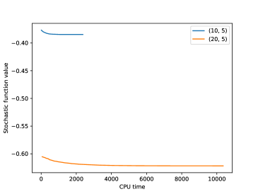
(a) Function value

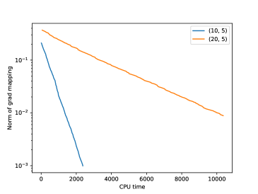
(b) Norm of the approximate gradient mapping

Figure 1: The convergence curve of applying Algorithm 3 to the robust Karcher mean problem (6.3). The CPU time is in seconds.

6.2 Robust maximum likelihood estimation

For the robust maximum likelihood estimation of the covariance matrix, one seeks to solve:

$$\min_{y\in\Delta_{n}}\ \left\|y-\frac{\mathbf{1}}{n}\right\|^{2}-\sum_{i=1}^{n}y_{i}\mathcal{L}(S;x_{i})$$ (6.5)

$$\text{ s.t. }X\in\mathop{\mathrm{missing}}{argmin}_{S\in\mathbb{S}^{d}_{++}}\ \sum_{i=1}^{n}y_{i}\mathcal{L}(S;x_{i}),$$

where $\mathcal{L}(S;x)$ is the log likelihood of the Gaussian distribution, namely

$$\mathcal{L}(S;\mathcal{D}):=\frac{1}{2}\mathop{\mathrm{missing}}{logdet}(S)+\frac{x^{\top}S^{-1}x}{2}.$$ (6.6)

Note that this lower level problem is geodesically strictly convex (see Sra and Hosseini (2015)), and thus has a unique solution. The calculations of the Riemannian gradient, Hessian-vector product and cross-derivatives all have closed form solutions (following Petersen et al. (2008)).

In the experiment, we test our algorithm with $d\in\{10,30,50\}$ and $n=100$. We repeat each dimension settings for 5 times and plot the average. The algorithm is terminated with $K=1000$ rounds of outer iterations, and the inner iteration is still taken to be $T=200$ (again a value which we observe a good inner iteration convergence). We take $\alpha_{k}=10^{-2}$ and $\beta_{k}=10^{-1}$. Figure 2 shows the results when applying RieBO to the above robust MLE problem with different choices of dimensions. It can be seen from Figure 2 that Algorithm 3 can efficiently decrease both the function values and the norm of gradient mappings. Also, here we are able to test and present the results for a much larger dimension due to much faster calculations of Riemannian gradients, Hessian-vector products and cross-derivatives.

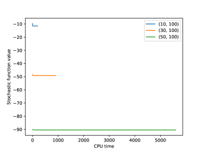
(a) Function value

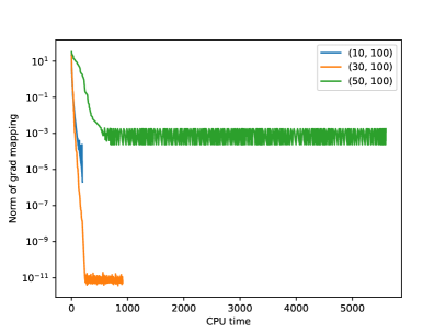
(b) Norm of the approximate gradient mapping

Figure 2: The convergence curve of Algorithm 3 applying to the robust covariance matrix maximum likelihood estimation problem (6.5) with different choice of $(d,n)$. The CPU time is in seconds.

7 Conclusion

We introduced the Riemannian bilevel optimization, a generalization of the traditional Euclidean bilevel optimization. We show that the Riemannian counterparts of Euclidean algorithms in Chen et al. (2021b); Ji et al. (2021) can achieve the same rate of convergence.

Our work raises several open questions. The first is how we can make the convergence independent of the sectional curvature of the manifold, similar to the results in Cai et al. (2023). It is also worth exploring the last iterate convergence of Riemannian bilevel problem. Last, it still needs investigation to see if there are efficient algorithms that can overcome the difficulty we mentioned in the numerical experiment part to efficiently calculate the Riemannian Hessian-vector product thus enabling large-scale implementation of algorithms for solving the Riemannian bilevel optimization problems.

References

• Bendory et al. (2017) T. Bendory, Y. C. Eldar, and N. Boumal. Non-convex phase retrieval from STFT measurements. IEEE Transactions on Information Theory, 64(1):467–484, 2017.
• Bhatia (2009) R. Bhatia. Positive definite matrices. Princeton university press, 2009.
• Bonnabel (2013) S. Bonnabel. Stochastic gradient descent on Riemannian manifolds. IEEE Transactions on Automatic Control, 58(9):2217–2229, 2013.
• Bonnel et al. (2015) H. Bonnel, L. Todjihoundé, and C. Udrişte. Semivectorial bilevel optimization on Riemannian manifolds. Journal of Optimization Theory and Applications, 167(2):464–486, 2015.
• Boumal (2023) N. Boumal. An introduction to optimization on smooth manifolds. Cambridge University Press, 2023.
• Boumal and Absil (2011) N. Boumal and P. Absil. RTRMC: A Riemannian trust-region method for low-rank matrix completion. In Advances in neural information processing systems, pages 406–414, 2011.
• Boumal et al. (2018) N. Boumal, P.-A. Absil, and C. Cartis. Global rates of convergence for nonconvex optimization on manifolds. IMA Journal of Numerical Analysis, 39(1):1–33, 2018.
• Bracken and McGill (1973) J. Bracken and J. T. McGill. Mathematical programs with optimization problems in the constraints. Operations Research, 21(1):37–44, 1973.
• Cai et al. (2023) Y. Cai, M. I. Jordan, T. Lin, A. Oikonomou, and E.-V. Vlatakis-Gkaragkounis. Curvature-independent last-iterate convergence for games on Riemannian manifolds. arXiv preprint arXiv:2306.16617, 2023.
• Chen et al. (2023a) L. Chen, J. Xu, and J. Zhang. On bilevel optimization without lower-level strong convexity. arXiv preprint arXiv:2301.00712, 2023a.
• Chen et al. (2017) R. Chen, B. Lucier, Y. Singer, and V. Syrgkanis. Robust optimization for non-convex objectives. arXiv preprint arXiv:1707.01047, 2017.
• Chen et al. (2021a) T. Chen, Y. Sun, and W. Yin. A single-timescale stochastic bilevel optimization method. arXiv preprint arXiv:2102.04671, 2021a.
• Chen et al. (2021b) T. Chen, Y. Sun, and W. Yin. Tighter analysis of alternating stochastic gradient method for stochastic nested problems. arXiv preprint arXiv:2106.13781, 2021b.
• Chen et al. (2022) X. Chen, M. Huang, and S. Ma. Decentralized bilevel optimization. arXiv preprint arXiv:2206.05670, 2022.
• Chen et al. (2023b) X. Chen, M. Huang, S. Ma, and K. Balasubramanian. Decentralized stochastic bilevel optimization with improved per-iteration complexity. In International Conference on Machine Learning, pages 4641–4671. PMLR, 2023b.
• Cherian and Sra (2016) A. Cherian and S. Sra. Riemannian dictionary learning and sparse coding for positive definite matrices. IEEE transactions on neural networks and learning systems, 28(12):2859–2871, 2016.
• Daskalakis and Panageas (2018) C. Daskalakis and I. Panageas. The limit points of (optimistic) gradient descent in min-max optimization. Advances in Neural Information Processing Systems, 31, 2018.
• Domke (2012) J. Domke. Generic methods for optimization-based modeling. In Artificial Intelligence and Statistics, pages 318–326. PMLR, 2012.
• Dong et al. (2023) Y. Dong, S. Ma, J. Yang, and C. Yin. A single-loop algorithm for decentralized bilevel optimization. arXiv preprint arXiv:2311.08945, 2023.
• Ferreira et al. (2019) O. P. Ferreira, M. S. Louzeiro, and L. Prudente. Gradient method for optimization on Riemannian manifolds with lower bounded curvature. SIAM Journal on Optimization, 29(4):2517–2541, 2019.
• Flamary et al. (2014) R. Flamary, A. Rakotomamonjy, and G. Gasso. Learning constrained task similarities in graph regularized multi-task learning. Regularization, Optimization, Kernels, and Support Vector Machines, 103, 2014.
• Franceschi et al. (2018) L. Franceschi, P. Frasconi, S. Salzo, R. Grazzi, and M. Pontil. Bilevel programming for hyperparameter optimization and meta-learning. In International Conference on Machine Learning, pages 1568–1577. PMLR, 2018.
• Ghadimi and Wang (2018) S. Ghadimi and M. Wang. Approximation methods for bilevel programming. arXiv preprint arXiv:1802.02246, 2018.
• Gould et al. (2016) S. Gould, B. Fernando, A. Cherian, P. Anderson, R. S. Cruz, and E. Guo. On differentiating parameterized argmin and argmax problems with application to bi-level optimization. arXiv preprint arXiv:1607.05447, 2016.
• Grazzi et al. (2020) R. Grazzi, L. Franceschi, M. Pontil, and S. Salzo. On the iteration complexity of hypergradient computation. In International Conference on Machine Learning, pages 3748–3758. PMLR, 2020.
• Han et al. (2023) A. Han, B. Mishra, P. Jawanpuria, P. Kumar, and J. Gao. Riemannian Hamiltonian methods for min-max optimization on manifolds. SIAM Journal on Optimization, 33(3):1797–1827, 2023.
• Harandi et al. (2017) M. Harandi, M. Salzmann, and R. Hartley. Dimensionality reduction on SPD manifolds: The emergence of geometry-aware methods. IEEE transactions on pattern analysis and machine intelligence, 40(1):48–62, 2017.
• Hayami (2018) K. Hayami. Convergence of the conjugate gradient method on singular systems. arXiv preprint arXiv:1809.00793, 2018.
• Hong et al. (2020) M. Hong, H.-T. Wai, Z. Wang, and Z. Yang. A two-timescale framework for bilevel optimization: Complexity analysis and application to actor-critic. arXiv preprint arXiv:2007.05170, 2020.
• Huang et al. (2020) F. Huang, S. Gao, and H. Huang. Gradient descent ascent for min-max problems on Riemannian manifolds. arXiv preprint arXiv:2010.06097, 2020.
• Ji and Liang (2021) K. Ji and Y. Liang. Lower bounds and accelerated algorithms for bilevel optimization. arXiv preprint arXiv:2102.03926, 2021.
• Ji et al. (2020) K. Ji, J. D. Lee, Y. Liang, and H. V. Poor. Convergence of meta-learning with task-specific adaptation over partial parameters. Advances in Neural Information Processing Systems, 33:11490–11500, 2020.
• Ji et al. (2021) K. Ji, J. Yang, and Y. Liang. Bilevel optimization: Convergence analysis and enhanced design. In International Conference on Machine Learning, pages 4882–4892. PMLR, 2021.
• Jin et al. (2020) C. Jin, P. Netrapalli, and M. Jordan. What is local optimality in nonconvex-nonconcave minimax optimization? In International Conference on Machine Learning, pages 4880–4889. PMLR, 2020.
• Kasai et al. (2018) H. Kasai, H. Sato, and B. Mishra. Riemannian stochastic recursive gradient algorithm. In International Conference on Machine Learning, pages 2516–2524, 2018.
• Khanduri et al. (2021) P. Khanduri, S. Zeng, M. Hong, H.-T. Wai, Z. Wang, and Z. Yang. A near-optimal algorithm for stochastic bilevel optimization via double-momentum. Advances in neural information processing systems, 34:30271–30283, 2021.
• Konda and Tsitsiklis (1999) V. Konda and J. Tsitsiklis. Actor-critic algorithms. Advances in neural information processing systems, 12, 1999.
• Kunapuli et al. (2008) G. Kunapuli, K. P. Bennett, J. Hu, and J.-S. Pang. Classification model selection via bilevel programming. Optimization Methods & Software, 23(4):475–489, 2008.
• Lee (2006) J. M. Lee. Riemannian manifolds: an introduction to curvature, volume 176. Springer Science & Business Media, 2006.
• Li et al. (2020) J. Li, B. Gu, and H. Huang. Improved bilevel model: Fast and optimal algorithm with theoretical guarantee. arXiv preprint arXiv:2009.00690, 2020.
• Liao et al. (2018) R. Liao, Y. Xiong, E. Fetaya, L. Zhang, K. Yoon, X. Pitkow, R. Urtasun, and R. Zemel. Reviving and improving recurrent back-propagation. In International Conference on Machine Learning, pages 3082–3091. PMLR, 2018.
• Lin et al. (2017) L. Lin, B. St. Thomas, H. Zhu, and D. B. Dunson. Extrinsic local regression on manifold-valued data. Journal of the American Statistical Association, 112(519):1261–1273, 2017.
• Lin et al. (2020a) L. Lin, D. Lazar, B. Sarpabayeva, and D. B. Dunson. Robust optimization and inference on manifolds. arXiv preprint arXiv:2006.06843, 2020a.
• Lin et al. (2020b) T. Lin, C. Jin, and M. Jordan. On gradient descent ascent for nonconvex-concave minimax problems. In International Conference on Machine Learning, pages 6083–6093. PMLR, 2020b.
• Liu et al. (2020) R. Liu, P. Mu, X. Yuan, S. Zeng, and J. Zhang. A generic first-order algorithmic framework for bi-level programming beyond lower-level singleton. In International Conference on Machine Learning, pages 6305–6315. PMLR, 2020.
• Lorraine et al. (2020) J. Lorraine, P. Vicol, and D. Duvenaud. Optimizing millions of hyperparameters by implicit differentiation. In International Conference on Artificial Intelligence and Statistics, pages 1540–1552. PMLR, 2020.
• Maclaurin et al. (2015) D. Maclaurin, D. Duvenaud, and R. Adams. Gradient-based hyperparameter optimization through reversible learning. In International conference on machine learning, pages 2113–2122. PMLR, 2015.
• Mishra et al. (2019) B. Mishra, H. Kasai, P. Jawanpuria, and A. Saroop. A Riemannian gossip approach to subspace learning on Grassmann manifold. Machine Learning, pages 1–21, 2019.
• Mokhtari et al. (2020) A. Mokhtari, A. Ozdaglar, and S. Pattathil. A unified analysis of extra-gradient and optimistic gradient methods for saddle point problems: Proximal point approach. In International Conference on Artificial Intelligence and Statistics, pages 1497–1507. PMLR, 2020.
• Moore (2010) G. M. Moore. Bilevel programming algorithms for machine learning model selection. Rensselaer Polytechnic Institute, 2010.
• Nouiehed et al. (2019) M. Nouiehed, M. Sanjabi, T. Huang, J. D. Lee, and M. Razaviyayn. Solving a class of non-convex min-max games using iterative first order methods. Advances in Neural Information Processing Systems, 32, 2019.
• Okuno et al. (2021) T. Okuno, A. Takeda, A. Kawana, and M. Watanabe. On lp-hyperparameter learning via bilevel nonsmooth optimization. Journal of Machine Learning Research, 22(245):1–47, 2021.
• Pedregosa (2016) F. Pedregosa. Hyperparameter optimization with approximate gradient. In International conference on machine learning, pages 737–746. PMLR, 2016.
• Petersen et al. (2008) K. B. Petersen, M. S. Pedersen, et al. The matrix cookbook. Technical University of Denmark, 7(15):510, 2008.
• Rajeswaran et al. (2019) A. Rajeswaran, C. Finn, S. M. Kakade, and S. Levine. Meta-learning with implicit gradients. Advances in neural information processing systems, 32, 2019.
• Shaban et al. (2019) A. Shaban, C.-A. Cheng, N. Hatch, and B. Boots. Truncated back-propagation for bilevel optimization. In The 22nd International Conference on Artificial Intelligence and Statistics, pages 1723–1732. PMLR, 2019.
• Shi et al. (2005) C. Shi, J. Lu, and G. Zhang. An extended Kuhn–Tucker approach for linear bilevel programming. Applied Mathematics and Computation, 162(1):51–63, 2005.
• Sra and Hosseini (2015) S. Sra and R. Hosseini. Conic geometric optimization on the manifold of positive definite matrices. SIAM Journal on Optimization, 25(1):713–739, 2015.
• Stackelberg and Peacock (1952) H. v. Stackelberg and A. T. Peacock. The theory of the market economy. (No Title), 1952.
• Sun et al. (2016) J. Sun, Q. Qu, and J. Wright. Complete dictionary recovery over the sphere ii: Recovery by Riemannian trust-region method. IEEE Transactions on Information Theory, 63(2):885–914, 2016.
• Sun et al. (2018) J. Sun, Q. Qu, and J. Wright. A geometric analysis of phase retrieval. Foundations of Computational Mathematics, 18(5):1131–1198, 2018.
• Tarzanagh et al. (2022) D. A. Tarzanagh, M. Li, C. Thrampoulidis, and S. Oymak. Fednest: Federated bilevel, minimax, and compositional optimization. In International Conference on Machine Learning, pages 21146–21179. PMLR, 2022.
• Tripuraneni et al. (2018) N. Tripuraneni, N. Flammarion, F. Bach, and M. I. Jordan. Averaging stochastic gradient descent on Riemannian manifolds. In Conference On Learning Theory, pages 650–687, 2018.
• Tu (2011) L. W. Tu. An Introduction to Manifolds. Springer Science & Universitext, 2011.
• Vandereycken (2013) B. Vandereycken. Low-rank matrix completion by Riemannian optimization. SIAM Journal on Optimization, 23(2):1214–1236, 2013.
• Weber and Sra (2019) M. Weber and S. Sra. Nonconvex stochastic optimization on manifolds via Riemannian Frank-Wolfe methods. arXiv preprint arXiv:1910.04194, 2019.
• Weber and Sra (2022) M. Weber and S. Sra. Projection-free nonconvex stochastic optimization on Riemannian manifolds. IMA Journal of Numerical Analysis, 42(4):3241–3271, 2022.
• Weber and Sra (2023) M. Weber and S. Sra. Riemannian optimization via Frank-Wolfe methods. Mathematical Programming, 199(1-2):525–556, 2023.
• Yang et al. (2023) Y. Yang, P. Xiao, and K. Ji. Achieving $\mathcal{O}(\epsilon^{-1.5})$ complexity in hessian/jacobian-free stochastic bilevel optimization. In Thirty-seventh Conference on Neural Information Processing Systems, 2023. URL https://openreview.net/forum?id=OzjBohmLvE.
• Yoon and Ryu (2021) T. Yoon and E. K. Ryu. Accelerated algorithms for smooth convex-concave minimax problems with $\mathcal{O}(1/k^{2})$ rate on squared gradient norm. In International Conference on Machine Learning, pages 12098–12109. PMLR, 2021.
• Yu and Zhu (2020) T. Yu and H. Zhu. Hyper-parameter optimization: A review of algorithms and applications. arXiv preprint arXiv:2003.05689, 2020.
• Zhang and Sra (2016) H. Zhang and S. Sra. First-order methods for geodesically convex optimization. In Conference on Learning Theory, pages 1617–1638. PMLR, 2016.
• Zhang et al. (2016) H. Zhang, S. J. Reddi, and S. Sra. Fast stochastic optimization on Riemannian manifolds. ArXiv e-prints, pages 1–17, 2016.
• Zhou et al. (2019) P. Zhou, X. Yuan, S. Yan, and J. Feng. Faster first-order methods for stochastic non-convex optimization on Riemannian manifolds. IEEE transactions on pattern analysis and machine intelligence, 2019.