Robust Multi-Task Learning with Excess Risks

Abstract

Multi-task learning (MTL) considers learning a joint model for multiple tasks by optimizing a convex combination of all task losses. To solve the optimization problem, existing methods use an adaptive weight updating scheme, where task weights are dynamically adjusted based on their respective losses to prioritize difficult tasks. However, these algorithms face a great challenge whenever label noise is present, in which case excessive weights tend to be assigned to noisy tasks that have relatively large Bayes optimal errors, thereby overshadowing other tasks and causing performance to drop across the board. To overcome this limitation, we propose Multi-Task Learning with Excess Risks (ExcessMTL), an excess risk-based task balancing method that updates the task weights by their distances to convergence instead. Intuitively, ExcessMTL assigns higher weights to worse-trained tasks that are further from convergence. To estimate the excess risks, we develop an efficient and accurate method with Taylor approximation. Theoretically, we show that our proposed algorithm achieves convergence guarantees and Pareto stationarity. Empirically, we evaluate our algorithm on various MTL benchmarks and demonstrate its superior performance over existing methods in the presence of label noise.

1 Introduction

Multi-task learning (MTL) aims to train a single model to perform multiple related tasks (Caruana, 1997). Due to the nature of learning multiple tasks simultaneously, the problem is often tackled by aggregating multiple objectives into a scalar one via a convex combination. Despite various efforts to achieve more balanced training, a crucial aspect that often remains overlooked is robustness to label noise. Label noise is ubiquitous in real-world MTL problems as the tasks are drawn from diverse sources, introducing variations in data quality (Hsieh and Tseng, 2021; Burgert et al., 2022). The presence of label noise can negatively impact the performance of all tasks trained jointly, leading to sub-optimal performance across the board. Addressing this issue is essential for the robust and reliable deployment of MTL models in real-world scenarios.

In this work, we study label noise in MTL by delving into a practical scenario where one or more tasks are contaminated by label noise due to the heterogeneity of data collection processes. Under label noise, scalarization (static weighted combination) is not robust because it overlooks the dataset quality. In fact, scalarization is prone to overfitting to a subset of tasks so that it cannot achieve a balanced solution among tasks, especially for under-parametrized models (Hu et al., 2023). Similarly, existing adaptive weight updating methods are vulnerable to label noise. These methods aim at prioritizing difficult tasks during training, and the difficulty is typically measured by the magnitude of each task loss (Chen et al., 2018; Liu et al., 2019; Sagawa et al., 2020; Liu et al., 2021c). Namely, they assign higher weights to the tasks with higher losses. However, the high loss may stem from label noise rather than insufficient training. For instance, if a task has noise in labels, its loss will be high, yet it provides no informative signal for the learning process.

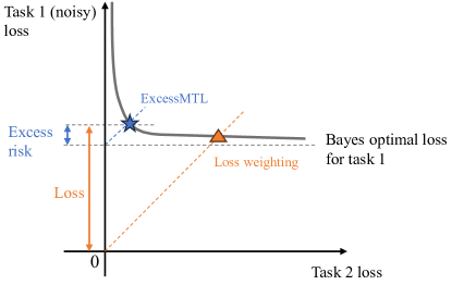
Figure 1: Conceptual comparison between ExcessMTL and loss weighting methods. The figure shows a two-task MTL setting, where Task 1 contains label noise, while Task 2 does not. Thus, the Bayes optimal loss (dashed line) for Task 1 is non-zero. The curve represents the Pareto front, i.e., all points on the curve are Pareto optimal. Loss weighting methods aim to find the solution with equal losses for two tasks, severely sacrificing the performance of Task 2. On the other hand, ExcessMTL finds the solution with equal excess risks, striking a better balance between the two tasks.

To address this challenge, we propose Multi-Task Learning with Excess Risks (ExcessMTL), which is robust to label noise while retaining the benefit of prioritizing worse-trained tasks. It dynamically adjusts the task weights based on their distance to convergence. Specifically, we define the distance to be excess risks, which measure the gap of loss between the current model and the optimal model in the hypothesis class. In the presence of different noise levels among tasks, the converged task-specific losses are likely to differ and are not guaranteed to be low. On the other hand, with proper training, excess risks for all tasks will approach 0. Thus, excess risks provide the true improvement ceiling achievable through model training or refinement, making it naturally robust to label noise by definition. The advantage of excess risks over losses as a difficulty measure is demonstrated in Figure 1. Since the optimal loss is usually intractable to compute, we propose an efficient method to estimate excess risks via Taylor approximation.

At a high level, ExcessMTL iteratively executes the following steps until convergence: i) estimate excess risk for each task, ii) update task weights based on their respective excess risks, iii) perform a gradient update using the weighted sum of losses. The ability to identify the convergence distance leads to robustness in the presence of label noise. Even if one or multiple tasks are highly corrupted by label noise, the overall performance will not be compromised.

Theoretically, we derive convergence guarantees for our algorithm and establish connections with multi-objective optimization, proving that the solutions of ExcessMTL are Pareto stationary. Empirically, we evaluate our method on various MTL benchmarks, showing that it outperforms existing adaptive weighting methods in the presence of label noise, even in cases of extreme noise in one or a few tasks. Our results highlight the robustness of excess risk-based weighting methods, especially when label noise is a concern.

2 Preliminaries

2.1 Excess Risks

Consider predicting the label $y\in\mathcal{Y}$ from the input data $x\in\mathcal{X}$. Let the data be drawn from some distribution $P$. Given a loss function $\ell$, the risk (or expected loss) of a model $\theta$ from the model family $\Theta$ is given by

$$\varepsilon(\theta)=\mathbb{E}_{(x,y)\sim P}[\ell(\theta;(x,y))].$$

The risk can be further decomposed as follows

$$\varepsilon(\theta)=\underbrace{\underbrace{\varepsilon(\theta)-\varepsilon(\theta_{\Theta}^{*})}_{\text{Estimation error}}+\underbrace{\varepsilon(\theta_{\Theta}^{*})-\varepsilon(\theta^{*})}_{\text{Approximation error}}}_{\text{Excess risk}(\mathcal{E})}+\underbrace{\varepsilon(\theta^{*})}_{\text{Bayes error}},$$

where $\theta_{\Theta}^{*}=\operatornamewithlimits{argmin}_{\theta\in\Theta}\mathbb{E}_{(x,y)\sim P}[\ell(\theta;(x,y))]$ is the optimal model in the model family $\Theta$ and $\theta^{*}=\operatornamewithlimits{argmin}_{\theta}\mathbb{E}_{(x,y)\sim P}[\ell(\theta;(x,y))]$ is the optimal model in any model family. The combination of estimation error and approximation error is the excess risk, denoted as $\mathcal{E}$. When the function class $\mathcal{F}$ is expressive enough, the approximation error approaches 0. The Bayes error is irreducible due to the stochasticity in the data generating process (e.g., label noise). For instance, if the data generating process is non-deterministic, one data point can have non-zero probability of belonging to multiple classes. This is an inherent property of a dataset, where high label noise leads to high Bayes error. On the other hand, the excess risk captures the difference between the risks of the model and the Bayes optimal model, effectively removing the influence of label noise. Therefore, it can be viewed as a measure of distance to optimality.

The above decomposition of risk highlights that it is not an appropriate criterion for evaluating model performance because it incorporates the irreducible error, which heavily depends on the noise level in the dataset. Since we typically do not have control over the dataset quality, excess risk is a more robust measure of model performance, particularly in the presence of label noise. It allows us to focus on the part of risk that can be improved through model learning and optimization, making it a reliable metric for assessing the effectiveness of models.

2.2 Multi-task Learning

In MTL, $m\geq 2$ tasks are given. We use $\alpha_{i}$ to represent the weight of the $i$th task and $\Delta_{m}$ to denote the $(m-1)$-dimensional probability simplex. We study the setting of hard parameter sharing, where a subset of model parameters ($\theta_{sh}$) is shared across all tasks, while other parameters ($\theta_{i}$) are task-specific. The goal of MTL is to find the parameter $\theta_{sh}$ and $\theta_{i}$ that minimizes a convex combination of all task-specific losses ($\ell_{i}$)

$$\min_{\theta_{sh},\theta_{1},\cdots\theta_{m}}\sum_{i=1}^{m}\alpha_{i}\ell_{i}(\theta_{sh},\theta_{i}),$$ (1)

where $\alpha_{i}\in\Delta_{m}$. The weights can be either static (Liu et al., 2021a; Yu et al., 2020) or dynamically computed (Chen et al., 2018; Liu et al., 2019, 2021c; Navon et al., 2022).

Despite the wide usage of the weighted combination scheme, it is difficult to define optimality under the MTL setting because a model may work well on some tasks, but perform poorly on others. For more rigorous optimality analysis, MTL can be formulated as a multi-objective optimization problem (Sener and Koltun, 2018; Zhou et al., 2022), where two models can be compared by Pareto dominance.

Definition 2.1 (Pareto dominance).

Let $L(\theta)=\{\ell_{i}(\theta):i\in[m]\}$ be a set of loss functions. For two parameter vectors $\theta_{1}$ and $\theta_{2}$, if $\ell_{i}(\theta_{1})\leq\ell_{i}(\theta_{2})$ for all $i\in[m]$ and $L(\theta_{1})\neq L(\theta_{2})$, we say that $\theta_{1}$ Pareto dominates $\theta_{2}$ with the notation $\theta_{1}\prec\theta_{2}$.

The goal of multi-task learning as multi-objective optimization is to achieve Pareto optimality.

Definition 2.2 (Pareto optimal).

A parameter vector $\theta^{*}$ is Pareto optimal if there exists no parameter $\theta$ such that $\theta\prec\theta^{*}$.

There may exist multiple Pareto optimal solutions and they consist the Pareto set. A weaker condition is called Pareto stationary and all Pareto optimal points are Pareto stationary.

Definition 2.3 (Pareto stationary).

A parameter $\theta$ is called Pareto stationary if there exists $\alpha\in\Delta_{m}$ such that $\sum_{i=1}^{m}\alpha_{i}\nabla_{\theta}\ell_{i}(\theta)=0$.

3 Multi-Task Learning with Excess Risks

We now introduce our main algorithm. In Section 3.1, we begin by identifying a key limitation of previous MTL algorithms and outlining our objectives. In Section 3.2, we provide a detailed description of the algorithm. In Section 3.3, we make a conceptual comparison between our proposed algorithm with existing task weighting methods. Finally, in Section 3.4, we present a theoretical analysis of the convergence guarantee and Pareto stationarity of our algorithm.

3.1 Motivations and Objectives

Prior works have demonstrated that effective multi-task learning requires task balancing, i.e., tasks that the current model performs poorly on should be assigned higher weights during training (Guo et al., 2018; Kendall et al., 2018). One popular method is loss balancing, which assigns high weights to the tasks with high losses, in the hope of prioritizing difficult tasks and making the training more balanced. However, we argue that task-specific loss is not a good criterion for task difficulty, as it not only considers model training, but is also subject to the quality of the dataset, which we may not have prior knowledge about. For instance, the high loss may not necessarily stem from insufficient training, but from high label noise. In that case, assigning high weights to the noisy tasks can hurt the multi-task performance across the board.

To address this problem, we propose to use excess risks to weigh the tasks because it measures the true performance gap that can be closed by model training. We hope to assign high weights to tasks with high excess risks such that all tasks converge at similar rates. To achieve this goal, we solve the min-max problem

$$\min_{\theta_{sh},\theta_{1},\cdots\theta_{m}}\max_{i\in[m]}~{}\mathcal{E}_{i}(\theta_{sh},\theta_{i}),$$ (2)

where $\mathcal{E}_{i}$ is the excess risk of the $i$th task.

Algorithm 1 ExcessMTL

  Input: Step size $\eta_{\alpha}$, $\eta_{\theta}$, number of total tasks $m$

  Initialize $\theta_{sh}^{(1)}$ and $\theta_{i}^{(1)}$ for all $i\in[m]$, $\alpha^{(1)}=[1/m,\cdots,1/m]$

  for $t=1,2\cdots$ do

     for $i=1,\cdots,m$ do

        Compute gradient $g_{i}^{(t)}=\nabla_{\theta_{sh}}\ell_{i}^{(t)}(\theta_{sh},\theta_{i})$

        Compute excess risks with Eq. 6 and Eq. 7

        $\hat{\mathcal{E}}_{i}^{(t)}={g_{i}^{(t)}}^{\top}{\text{diag}\left(\sum_{\tau=1}^{t}g_{i}^{(\tau)}{g_{i}^{(\tau)}}^{\top}\right)^{-1/2}}g_{i}^{(t)}$

        Update weights $\alpha_{i}^{(t+1)}=\alpha_{i}^{(t)}\exp\left(\eta_{\alpha}\hat{\mathcal{E}}_{i}^{(t)}\right)$

        Update task-specific parameters

        $\theta^{(t+1)}_{i}\leftarrow\theta^{(t)}_{i}-\eta_{\theta}\nabla_{\theta_{i}}\ell_{i}^{(t)}(\theta_{sh},\theta_{i})$

     end for

     Normalize $\alpha_{i}^{(t+1)}\leftarrow\alpha_{i}^{(t+1)}/\sum_{j}\alpha_{j}^{(t+1)}$ for all $i$

     Update shared parameters

     $\theta^{(t+1)}_{sh}\leftarrow\theta^{(t)}_{sh}-\eta_{\theta}\sum_{i}\alpha_{i}^{(t+1)}\nabla_{\theta_{sh}}\ell_{i}^{(t)}(\theta_{sh},\theta_{i})$

  end for

3.2 Algorithm

We present our algorithm in Algorithm 1, which consists of three main components: excess risk estimation, multiplicative weight update, and scale processing.

Excess risks estimation. For the ease of presentation, we overload the expression $\theta_{i}$ as a combination of $\theta_{sh}$ and $\theta_{i}$ for task $i$. In the computation of excess risks, the Bayes optimal loss is generally intractable to compute exactly, so we propose to use a local approximation instead. Specifically, we use the second-order Taylor expansion of the task-specific loss $\ell_{i}$ at the current parameter $\theta_{i}^{(t)}$

$$\ell_{i} (\theta)=\ell_{i}(\theta_{i}^{(t)})+(\theta-\theta_{i}^{(t)})^{\top}g_{i}^{(t)}$$

$$+\frac{1}{2}(\theta-\theta_{i}^{(t)})^{\top}H_{i}^{(t)}(\theta-\theta_{i}^{(t)})+\mathcal{O}(\|\theta-\theta_{i}^{(t)}\|_{2}^{3}),$$ (3)

where $g_{i}^{(t)}$ is the gradient and $H_{i}^{(t)}$ is the Hessian matrix of $\ell_{i}$ at $\theta_{i}^{(t)}$. Plugging the locally optimal parameter $\theta_{i}^{*}$ in Eq. 3, we can estimate the excess risk as

$$\mathcal{E}_{i}(\theta_{i}^{(t)})\approx\ell_{i}(\theta_{i}^{(t)})-\ell_{i}(\theta_{i}^{*})$$

$$\approx (\theta_{i}^{(t)}-\theta_{i}^{*})^{\top}g_{i}^{(t)}-\frac{1}{2}(\theta_{i}^{(t)}-\theta_{i}^{*})^{\top}H_{i}^{(t)}(\theta_{i}^{(t)}-\theta_{i}^{*}).$$ (4)

To obtain the difference between $\theta_{i}^{(t)}$ and $\theta_{i}^{*}$, we use the fact that $\theta_{i}^{*}$ is locally optimal,

$$\nabla_{\theta_{i}^{*}}\ell_{i}(\theta_{i}^{*}) \approx g_{i}^{(t)}+H_{i}^{(t)}(\theta_{i}^{*}-\theta_{i}^{(t)})=0$$

$$\implies\theta_{i}^{(t)}-\theta_{i}^{*} \approx{H_{i}^{(t)}}^{-1}g_{i}^{(t)}.$$ (5)

Plugging Eq. 5 into Eq. 4 and assuming the second-order partial derivative is continuous, we have

$$\mathcal{E}_{i}(\theta_{i}^{(t)}) \approx\frac{1}{2}{g_{i}^{(t)}}^{\top}{H_{i}^{(t)}}^{-1}g_{i}^{(t)}.$$ (6)

The factor $1/2$ can be dropped for simplicity. However, the computation of the Hessian matrix is generally intractable, so we use the diagonal approximation of empirical Fisher (Amari, 1998) to estimate it, which computes a diagonal matrix through the accumulation of outer products of historical gradients. This approach has shown to be useful in various practical settings (Duchi et al., 2011; Kingma and Ba, 2015). Specifically, let $g_{i}^{(\tau)}$ be the gradient of the $i$th task with respect to the model parameter $\theta_{i}^{(\tau)}$ at time step $\tau$, the approximate Hessian at time step $t$ for the $i$th task is

$${H^{(t)}_{i}}\approx\text{diag}\left(\sum_{\tau=1}^{t}g_{i}^{(\tau)}{g_{i}^{(\tau)}}^{\top}\right)^{1/2},$$ (7)

where $\text{diag}(\cdot)$ is a diagonal matrix. The estimation is efficient as the computational complexity is $\mathcal{O}(d)$, where $d$ is the dimension of parameters.

Multiplicative weight update.  After estimating the excess risks, we update the task weights accordingly. As the gradients contain stochastic factors during the training, this online learning process calls for the stability of $\alpha$ for algorithmic convergence (Hazan et al., 2016). The one-hot solution in Equation 8 suffers from fluctuation and cannot be directly applied. Following the framework of online mirror descent with entropy regularization that formulates KL divergence as Bregman divergence (Hazan et al., 2016), we smooth out the hard choice of a single task with a weight vector $\alpha\in\Delta_{m}$, so problem 2 can be reformulated as

$$\min_{\theta_{sh},\theta_{1},\cdots\theta_{m}}\max_{\alpha\in\Delta_{m}}\sum_{i=1}^{m}\alpha_{i}\mathcal{E}_{i}(\theta_{sh},\theta_{i}).$$ (8)

Here we find the task weights $\alpha^{(t)}$ by

$$\alpha^{(t+1)}= \operatornamewithlimits{argmax}_{\alpha\in\Delta_{m}}\sum_{i=1}^{m}\alpha_{i}\mathcal{E}_{i}(\theta_{sh}^{(t)},\theta_{i}^{(t)})-\frac{1}{\eta_{\alpha}}\text{KL}(\alpha\|\alpha^{(t)}),$$

which can easily be proven as equivalent to

$$\alpha_{i}^{(t+1)}=\frac{\alpha_{i}^{(t)}\exp\left(\eta_{\alpha}\mathcal{E}_{i}(\theta_{sh}^{(t)},\theta_{i}^{(t)})\right)}{\sum_{j=1}^{m}\alpha_{j}^{(t)}\exp\left(\eta_{\alpha}\mathcal{E}_{j}(\theta_{sh}^{(t)},\theta_{j}^{(t)})\right)},$$ (9)

where $\eta_{\alpha}$ is the step size for weight update. Note that this update can be viewed as an exponentiated gradient (Kivinen and Warmuth, 1997) step on the convex combination of excess risks. Based on the updated task weights, we compute the loss by taking a convex combination of each task-specific loss and backpropagating the gradient. Multiplicative weight update provides stability in training and we show the convergence guarantees in Section 3.4.

Scale processing.  Similar to loss and gradient, the excess risk is also sensitive to the scale of tasks. The issue can manifest in two scenarios. The first one is when the type of loss is the same across all tasks, but the input data for each task varies in magnitude. A simple solution is to standardize all input data such that they have zero mean and unit variance. The second case is when the tasks employ different losses. For instance, the cosine loss has a maximum value of 1, while the squared loss can be unbounded. To ensure a fair comparison among tasks with varying losses, we propose to compute the relative excess risks. We adopt a similar method from Chen et al. (2018) to normalize excess risks by dividing the current value by the initial value, ensuring a range from 0 to 1.

3.3 Conceptual Comparison

In this section, we discuss the relationships and distinctions between our approach and prior task-balancing methods conceptually. We demonstrate the limitations of previous methods, especially in the presence of label noise. Empirical verification of the arguments is presented in Section 4.3.

GradNorm (Chen et al., 2018) enforces similar gradient norms and training rates across all tasks. The training rate is defined as the ratio of the current and the initial loss. It tends to favor tasks with small gradient norms, overlooking inherent scale differences in task gradients. In the face of label noise, noisy tasks inevitably exhibit a slow training rate due to their high losses. However, GradNorm treats this as insufficient training and assigns high weights to the noisy tasks. Additionally, the task weights require additional gradient updates as they are learnable parameters in GradNorm, whereas our algorithm does not.

MGDA (Sener and Koltun, 2018) formulates multi-task learning as multi-objective optimization. They solve it by using the classical multiple gradient descent algorithm (Mukai, 1980; Fliege and Svaiter, 2000; Désidéri, 2012), which finds the minimum norm within the convex hull of task gradients. It also tends to favor tasks with small gradient magnitudes due to the nature of the Frank-Wofle algorithm it employs. Consider two tasks with gradients $\|g_{1}\|_{2}>\|g_{2}\|_{2}$ where the projection of $g_{1}$ on $g_{2}$ has a larger norm than $g_{2}$. In this case, MGDA will concentrate all weights on task 2. This observation holds in general beyond the two-task example. As the loss landscape of a noisy task tends to be flatter, its gradient magnitude will be smaller, thus favored by MGDA. Moreover, the Frank-Wofle algorithm requires pairwise computation among all tasks, which is prohibitive under large number of tasks.

GroupDRO (Sagawa et al., 2020) is initially designed to address the problem of subpopulation shift and has since been extended to multi-task learning (Michel et al., 2021). It aims to optimize the worst task loss by assigning high weights to tasks with high losses. However, in the presence of label noise, tasks with high noise levels will exhibit persistently high losses, which leads GroupDRO to assign excessive weight to those tasks, thereby ignoring the other tasks and causing an overall performance decline.

IMTL (Liu et al., 2021c) achieves impartial learning by requiring the gradient update to have equal projection on each task. In a two-task scenario, this is equivalent to finding the angle bisector for the task-specific gradients, meaning that regardless of the gradient magnitude, each task exerts an equal influence on determining the final gradient direction. However, when confronted with label noise, the noisy gradient can substantially distort the final gradient direction, damping or even misguiding the training.

3.4 Theoretical Analysis

To validate the theoretical soundness of Algorithm 1, we analyze its convergence property. Algorithm 1 takes inspiration from the online mirror descent algorithm (Nemirovskij and Yudin, 1983), where the update of parameter $\theta$ and weights $\alpha$ corresponds to online gradient descent and online exponentiated gradient respectively. With established results (Nemirovski et al., 2009) in the online learning literature, we show that Algorithm 1 converges at the rate $\mathcal{O}(1/\sqrt{t})$.

Theorem 3.1 (Convergence).

Suppose (i) each task-specific loss $\ell_{i}$ is L-Lipschitz, (ii) $\ell_{i}$ is convex on the model parameter $\theta$, (iii) $\ell_{i}$ bounded by $B_{\ell}$ and (iv) $\|\theta\|_{2}$ is bounded by $B_{\theta}$. At time step $t$, let $\bar{\theta}^{(1:t)}\coloneqq\frac{1}{t}\sum_{\tau=1}^{t}{\theta^{(\tau)}}$, then

$$\mathbb{E}\left[\sum_{i=1}^{m}\alpha_{i}^{(t)}\mathcal{E}_{i}(\bar{\theta}^{(1:t)})\right]-\min_{\theta}\max_{\alpha\in\Delta_{m}}\sum_{i=1}^{m}\alpha_{i}\mathcal{E}_{i}(\theta)\leq 2m\sqrt{\frac{10(B_{\theta}^{2}L^{2}+B_{\ell}^{2}\log m)}{t}},$$

where $m$ is the number of tasks.

With the convergence analysis, we further deduce that the solution of Algorithm 1 is Pareto optimal in the convex setting.

Corollary 3.2 (Pareto Optimality).

Under the same conditions as Theorem 3.1, using the weights $\alpha$ output by Algorithm 1, we have

$$\mathbb{E}\left[\sum_{i=1}^{m}\alpha_{i}\mathcal{E}_{i}(\bar{\theta}^{(1:t)})\right]-\sum_{i=1}^{m}\alpha_{i}\mathcal{E}_{i}(\theta^{*})\leq 2m\sqrt{\frac{10(B_{\theta}^{2}L^{2}+B_{\ell}^{2}\log m)}{t}},$$

where $\theta^{*}$ is the Pareto optimal solution, i.e., $\theta^{*}=\operatornamewithlimits{argmin}_{\theta}\sum_{i=1}^{m}\alpha_{i}\mathcal{E}_{i}(\theta)$.

This condition is the same as Definition 2.2 because the weights $\alpha$ are positive, so any Pareto improvement over $\theta^{*}$ would increase the sum. The proof is in Appendix A. For non-convex cases, we next provide a stationary analysis.

Theorem 3.3 (Pareto Stationarity).

Suppose each task-specific loss $\ell_{i}$ is (i) L-Lipschitz (ii) G-Smooth and (iii) bounded by $B_{\ell}$. At time step $t$, using the weights $\alpha$ output by Algorithm 1, we have

$$\min_{k=1,\ldots,t}\mathbb{E}\left[\left\|\sum_{i=1}^{m}{\alpha_{i}^{(k)}}\nabla\ell_{i}(\theta^{(k)})\right\|^{2}_{2}\right]\leq 6m\sigma\sqrt{\frac{B_{\ell}G}{t}},$$ (10)

where $m$ is the number of tasks.

This shows that Algorithm 1 converges to a Pareto stationary point with the rate $\mathcal{O}(1/t^{1/4})$, matching the rate for single-objective SGD (Drori and Shamir, 2020). We also empirically show that the algorithm performs well under the non-convex setting in Section 4. The proof is in Appendix B.

4 Experiments

The experiments aim to investigate the following questions under different levels of noise injection: i) Does label noise significantly harm MTL performance? ii) Does ExcessMTL perform consistently with its theoretical properties? iii) In presence of label noise, does ExcessMTL maintain high overall performance? iv) If so, is this achieved by appropriately assigning weights to the noisy tasks? In the subsequent analysis, we provide affirmative answers to all the questions.

4.1 Datasets

MultiMNIST (Sabour et al., 2017) is a multi-task version of the MNIST dataset. Two randomly selected MNIST images are put on the top-left and bottom-right corners respectively to construct a new image. Noise is injected into the bottom-right corner task.

Office-Home (Venkateswara et al., 2017) consists of four image classification tasks: artistic images, clip art, product images, and real-world images. It contains 15,500 images over 65 classes. Noise is injected into the product image classification task.

NYUv2 (Silberman et al., 2012) consists of RGB-D indoor images. It contains 3 tasks: semantic segmentation, depth estimation, and surface normal prediction. Noise is injected into the semantic segmentation task.

4.2 Noise Injection Scheme

To replicate the real-world scenario where tasks come from heterogeneous sources with various quality, we inject label noise into one or more (but not all) tasks within the task batch. For classification problems, we adopt the common practice of introducing symmetric noise (Kim et al., 2019), which is generated by flipping the true label to any possible labels uniformly at random. For regression problems, we introduce additive Gaussian noise (Hu et al., 2020) with the variance equal to that of the original regression target. This approach ensures that the level of noise introduced is consistent with the statistical characteristics of the original data. We vary the noise level by changing the proportion of training data subject to the noise injection procedure, allowing us to measure the impact of increasing levels of noise on the performance of our algorithm. The test data remains clean.

In the following sections, we refer to the tasks with noise injection as noisy tasks and tasks without noise injection as clean tasks. The proportion of noisy data in the noisy task is referred to as noise level.

4.3 Empirical Analysis and Comparison

In this section, we use MultiMNIST and Office-Home as illustrative examples to analyze the behavior of ExcessMTL in detail and demonstrate its advantage comparing with other task weighting methods.

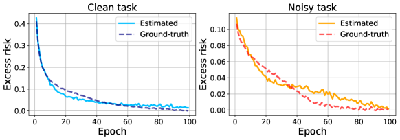
Figure 2: Excess risks on MultiMNIST with noise level 0.6. The estimated excess risk well matches the ground-truth pattern.

Excess risk estimation. We present the estimated excess risks on MultiMNIST in Fig. 2. Here, we use the difference between the current and converged loss as a proxy for the ground-truth excess risk. Initially, the noisy task shows lower excess risk due to higher Bayes optimal loss. As training proceeds, both tasks converge and excess risks approach 0. The estimation is up to a constant multiplier, so we scale the estimated value by a constant to align it with the ground-truth. Our estimated excess risk well matches the ground-truth pattern, validating its accuracy.

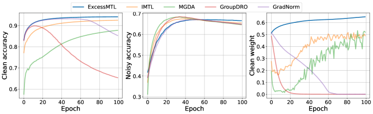
Figure 3: Weight and accuracy on the MultiMNIST dataset with a noise level of 0.8. ExcessMTL assigns most weight to the clean task so that the performance is least affected by the injected noise.

Training dynamics and weight assignment. We analyze the training dynamics for the algorithms mentioned in Section 3.3 in Figure 3. For each algorithm, we examine the change in task weights and test accuracy as training proceeds. GradNorm and GroupDRO rapidly assign substantial weights to the noisy task due to their high losses. IMTL and MGDA, on the other hand, initially allocate significant weights to the noisy task but eventually converge to nearly uniform weighting. Their emphasis on the noisy task dramatically impacts the performance of the clean task, leading to suboptimal performance.

In contrast, ExcessMTL identifies the higher excess risk associated with the clean task at the beginning of training, leading to a higher accumulation of weight on the clean task. Simultaneously, the reduced emphasis on the noisy task helps mitigate overfitting, leading to improved performance when learning with noise. This ability of ExcessMTL to assign appropriate weights based on the proximity to convergence contributes to its superior overall performance.

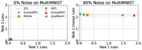
Figure 4: MultiMNIST loss profile (lower left better). The left plot has no noise injected, while in the right one, task 2 has 80% noise. With no noise injected, all algorithms achieve ideal performance. However, with significant noise injected, only ExcessMTL retains performance close to Bayes optimal on both tasks.

Performance comparison. In Figure 4, we present the converged performance of all algorithms with and without significant noise injection. When more noise is injected into task 2, its Bayes optimal loss increases, leading to a degradation in its single-task performance. A robust MTL algorithm should retain performance close to Bayes optimal regardless of noise level, i.e., reaching or surpassing the intersection of the single-task performance (dashed line). Despite performing well under the noise-free scenario, all algorithms except ExcessMTL have performance decrease in task 1 under label noise. The performance for loss weighting methods aligns with expectations in Figure 1, i.e., they aim for equal losses across both tasks, resulting in undertraining of task 1.

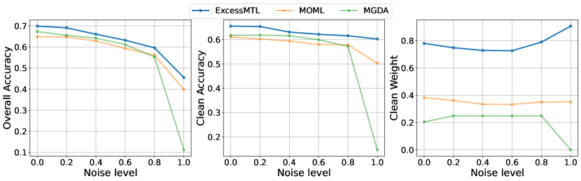
Figure 5: Comparison with MOML and MGDA. MGDA and MOML use the same method to select weights on training and validation set respectively. Despite more consistent weight assignment than MGDA, MOML fails when noise level is high, showing that a clean validation set does not alleviate the label noise issue. ExcessMTL ourperforms both baselines.

Clean validation set. One may expect that the existence of a clean validation set would address the label noise issue, as validation performance is a more robust metric than training loss. However, since weight selection on the validation set is performed on the clean data whereas the training set still contains noise, it could lead to assigning considerable weight to noisy tasks. To illustrate this possibility, we compare with MOML (Ye et al., 2021), which assigns weights using MGDA on a clean validation set. On the Office-Home dataset, we allocate $20\%$ of the training data as a clean validation set and inject noise into the remainder.

From Figure 5, despite the additional requirement of clean data, MOML remains largely impacted by label noise. When noise level is low, MOML performs worse than MGDA due to less gradient information contained in the validation set than the training set. When noise level is high, although MOML slightly improves over MGDA with more consistent weight assignment, the overall performance still significantly degrades. In contrast, ExcessMTL consistently outperforms both baselines, especially at high noise level.

4.4 Benchmark Evaluation

We present the results on three MTL benchmarks. For MultiMNIST and Office-Home, we present three plots: the overall performance, the average performance on the clean tasks and the sum of task weights assigned to the clean tasks, where the x-axis is the noise level. For NYUv2, we provide the performance of each task since they have different evaluation criteria. Along with adaptive weighting algorithms mentioned in Section 3.3, we also include uniform scalarization as a baseline.

The key evaluation criteria for robustness is that the performance on the clean tasks should not be affected even in face of increasing label noise in the noisy tasks.

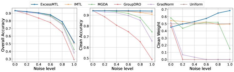
Figure 6: Results on the MultiMNIST dataset. Only ExcessMTL assigns smaller weights to the noisy task, maintaining the clean task accuracy, whereas other methods show decreasing performance.

MultiMNIST. From Figure 6, we can see that for all adaptive weighting methods except ExcessMTL, the performance on the clean task monotonically declines as the noise level increases. The weight plot indicates that this performance degradation stems from the excessive weights assigned to noisy tasks, and in extreme cases, the weight on the clean task is 0, effectively disregarding it during optimization. In contrast, ExcessMTL identifies and assigns minimal weights to the noisy task, preserving the performance on clean tasks even under high label noise (flat line in the clean accuracy plot).

Surprisingly, uniform scalarization also exhibits resilience to label noise, although slightly inferior to ExcessMTL. This can be attributed to the nature of MultiMNIST as an easy dataset with abundant data in the sense that two tasks have small interference with each other. Therefore, even if one task is fully corrupted, the clean task provides sufficient information to learn a model. However, we find that the performance of uniform scalarization is inconsistent and varies across datasets, as shown by the following experiments.

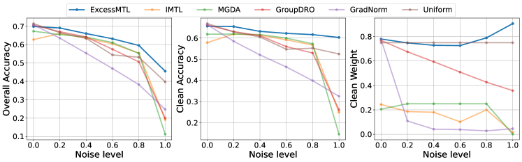
Figure 7: Results on the Office-Home dataset (noise in product classification). The left figure considers all tasks, while the other two consider all tasks except product images. The right figure is the combined weights of all clean tasks (0.75 for uniform scalarization). ExcessMTL is least affected by label noise and is the only adaptive algorithm assigning small weights to the noisy task.

Office-Home. Similar trends can be observed in Figure 7. The performance of ExcessMTL is least affected on the clean tasks, showcasing its robustness. When the noisy task has purely random label (noise level$=1$), all other adaptive methods completely fail. In contrast to the results in MultiMNIST, uniform scalarization is not sufficient to obtain good performance in this real-world dataset as it is outperformed by most adaptive weighting methods in the noisy setting. This underscores the need for adaptive methods in such scenarios.

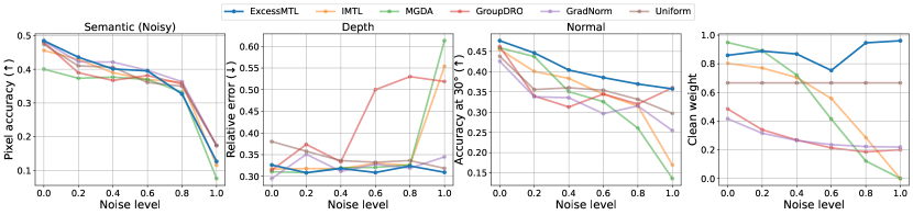
Figure 8: Results on the NYUv2 dataset (noise in semantic segmentation). Higher pixel accuracy for semantic segmentation ($\uparrow$), lower relative error for depth estimation ($\downarrow$) and higher angle accuracy for surface normal estimation ($\uparrow$) are desired. Pixel accuracy monotonically decreases as expected. ExcessMTL consistently achieves the best performance on the clean tasks, while other methods fail dramatically under high label noise.

NYUv2. From Figure 8, we observe that ExcessMTL consistently outperforms other methods on the two clean tasks. Other adaptive weighting algorithms assign increasing weights to the noisy task with rising noise level. The phenomenon is particularly evident when the noise level is high, confirming our hypothesis that label noise leads to suboptimal performance for all tasks trained jointly. Since the loss magnitude of the surface normal estimation task is the smallest, GroupDRO and uniform scalarization exhibit clear undertraining on it even without noise injection. Through our scale processing method, ExcessMTL evaluates the excess risks on a comparable scale and trains on all tasks in a more balanced way.

In summary, the experiments validate our hypothesis that label noise affects not only the noisy tasks, but also all tasks trained jointly, leading to an overall decline in performance. Compared with other adaptive weighting methods, ExcessMTL consistently achieves high overall performance by appropriately assigning weights to noisy tasks, thereby mitigating the negative impact of label noise. Notably, ExcessMTL maintains competitive performance with other methods in noise-free scenarios, indicating that its robustness does not come at the cost of performance degradation.

5 Related Work

MTL Optimization can be tackled from multiple perspectives. One line of work focuses on network architecture design (Dai et al., 2016; Liu et al., 2019). Another approach is gradient manipulation, where Chen et al. (2020) drops gradient components by the extent of conflict; Yu et al. (2020) removes gradient conflict by projection; Liu et al. (2021a) minimizes average loss while tracking the improvement on the worst task. Researchers have also studied the problem from a game theory perspective (Navon et al., 2022). In this study, our primary focus lies on task weighting methods (Kendall et al., 2018; Chen et al., 2018; Sener and Koltun, 2018; Liu et al., 2021c; Lin et al., 2022).

Task weighting is a common strategy employed to prioritize tasks with inferior performance. Existing algorithms in this domain differ in their measures of task difficulty, including homoscedastic uncertainty (Kendall et al., 2018), task-specific performance measures (Guo et al., 2018), norms of gradients and training rates (Chen et al., 2018), or a combination of task-specific losses and gradients (Liu et al., 2021c). Another approach formulates the MTL problem as a multi-objective optimization problem (Sener and Koltun, 2018) and utilizes the classical multiple-gradient descent algorithm (MGDA) (Mukai, 1980; Fliege and Svaiter, 2000; Désidéri, 2012) to find Pareto stationary solutions. While MGDA does not explicitly use gradient norms for task weighting, it implicitly considers them by seeking the minimum norm point within the convex hull of task gradients.

However, the problem of label noise is often overlooked in the existing works, which can make many proposed task difficulty measures inappropriate. For instance, high label noise will lead to high losses and potentially small gradient magnitudes, making aforementioned algorithms assign high weights to the noisy tasks and causing an imbalance in training. Our work incorporates the idea of prioritizing difficult tasks, while further improves the robustness to label noise.

Loss weighting in other applications. Beyond MTL, various machine learning problems employ similar mechanism of focusing on challenging samples, often utilizing loss as a difficulty measure. In domain generalization, prior works focus on domains or groups with higher losses to improve generalization (Sagawa et al., 2020; Liu et al., 2021b; Piratla et al., 2021). In hard example mining, researchers use losses to determine whether specific data instances are difficult for the model (Shrivastava et al., 2016; Yuan et al., 2017; Xue et al., 2019). Similar to MTL, those applications also suffer from the label noise problem. We believe our proposed method can offer a more robust difficulty measure for such applications. This extension of our methodology can pave the way for more reliable solutions across a spectrum of machine learning challenges.

6 Conclusion

In this work, we identify a key limitation of existing adaptive weight updating methods in multi-task learning, i.e., the vulnerability to label noise. Building upon this observation, we propose ExcessMTL, a task balancing algorithm based on excess risks. It employs multiplicative weight update to dynamically adjust the task weights according to their respective distance to convergence. We further show the convergence guarantees of the proposed algorithm and establish connections with multi-objective optimization, showing the Pareto stationarity of its solutions. Extensive experiments across diverse MTL benchmarks demonstrate the consistent superiority of our method in the presence of label noise. Beyond multi-task learning, our insights on excess risks and their connection with convergence distance can potentially inspire more robust algorithmic design in various machine learning applications utilizing loss weighting methods.

Appendix A Proof for Pareto Optimality

See 3.1

Proof.

We directly apply the well-established regret bound for online mirror descent from Nemirovski et al. [2009] on the saddle point problem

$$\min_{\theta\in\Theta}\max_{\alpha\in\Delta_{m}}\sum_{i=1}^{m}\alpha_{i}f_{i}(\theta).$$

In our case, $f_{i}(\cdot)$ is the excess risk for the $i$th task $\mathcal{E}_{i}(\cdot)$. We take inspiration from the proof strategy of Proposition 2 in Sagawa et al. [2020] to first present the bound and then explain why our formulation satisfies all conditions for the bound.

Assumption A.1.

$f_{i}$ is convex on $\Theta$.

Assumption A.2.

Let $\xi$ be a random vector that takes value in $\Xi$. For all $i\in[m]$, there exists a function $F_{i}:\Theta\times\Xi\rightarrow\mathbb{R}$ such that $\mathbb{E}_{\xi\sim p}[F_{i}(\theta;\xi)]=f_{i}(\theta)$.

Assumption A.3.

For every given $\theta\in\Theta$ and $\xi\in\Xi$, we are able to compute $F_{i}(\theta,\xi)$ and the subgradient $\nabla F_{i}(\theta,\xi)$ such that $\mathbb{E}_{\xi\sim p}[\nabla F_{i}(\theta,\xi)]=\nabla f_{i}(\theta)$, $\mathbb{E}_{\xi\sim p}[\|\nabla F_{i}(\theta,\xi)-\nabla f_{i}(\theta)\|]\leq\sigma$.

Theorem A.4 (Nemirovski et al. 2009).

If Assumption 1-3 hold, at time step $t$, the regret for the online mirror descent algorithm on the saddle point problem

$$\min_{\theta\in\Theta}\max_{\alpha\in\Delta_{m}}\sum_{i=1}^{m}\alpha_{i}f_{i}(\theta)$$

can be bounded by

$$\mathbb{E}\left[\max_{\alpha\in\Delta_{m}}\sum_{i=1}^{m}\alpha_{i}f_{i}(\bar{\theta}^{(1:t)})-\min_{\theta\in\Theta}\sum_{i=1}^{m}\bar{\alpha_{i}}^{(1:t)}f_{i}(\theta)\right]\leq 2\sqrt{\frac{10(R_{\theta}^{2}M^{2}_{*,\theta}+M^{2}_{*,\alpha}\log m)}{t}},$$

where

$$\mathbb{E}\left[\left\|\nabla_{\theta}\sum_{i=1}^{m}\alpha_{i}F_{i}(\theta;\xi)\right\|^{2}_{*,\theta}\right]\leq M_{*,\theta},$$

$$\mathbb{E}\left[\left\|\nabla_{\alpha}\sum_{i=1}^{m}\alpha_{i}F_{i}(\theta;\xi)\right\|^{2}_{*,\alpha}\right]\leq M_{*,\alpha},$$

$$R_{\theta}^{2}=\frac{1}{c}(\max_{\theta}\|\theta\|^{2}_{\theta}-\min_{\theta}\|\theta\|^{2}_{\theta})$$

for a $c-$strongly convex norm $\|\cdot\|_{\theta}$.

Assumption A.1 is the same as our condition (ii). For Assumption A.2, we can let $\xi$ be the tuple $(x,y,i)$, where $i$ is the task index. Then, let the distribution of $\xi$ can be a mixture of each task distribution $P_{i}$, i.e.,

$$p\coloneqq\frac{1}{m}\sum_{i=1}^{m}P_{i}.$$

To make $F_{i}$ an unbiased estimator for $f_{i}$, we construct

$$F_{i}(\theta;(x,y,i^{\prime}))\coloneqq m\mathbbm{1}[i=i^{\prime}]f_{i}(\theta).$$

We can check the validity of this construction by

$$\mathbb{E}_{(x,y,i^{\prime})\sim p}[F_{i}(\theta;(x,y,i^{\prime}))]=\frac{1}{m}\mathbb{E}_{P_{i}}[mf_{i}(\theta)]=f_{i}(\theta).$$

For Assumption A.3, similarly,

$$\mathbb{E}_{(x,y,i^{\prime})\sim p}[\nabla F_{i}(\theta;(x,y,i^{\prime}))]=\frac{1}{m}\mathbb{E}_{P_{i}}[m\nabla f_{i}(\theta)]=\nabla f_{i}(\theta).$$

According to our condition (iii) and (iv), we have that

$$\mathbb{E}\left[\left\|\nabla_{\theta}\sum_{i=1}^{m}\alpha_{i}F_{i}(\theta;(x,y,i^{\prime}))\right\|^{2}_{*,\theta}\right]\leq m^{2}L^{2}=M_{*,\theta},$$

$$\mathbb{E}\left[\left\|\nabla_{\alpha}\sum_{i=1}^{m}\alpha_{i}F_{i}(\theta;\xi)\right\|^{2}_{*,\alpha}\right]\leq m^{2}B_{\ell}^{2}=M_{*,\alpha},$$

$$R_{\theta}^{2}=\frac{1}{c}(\max_{\theta}\|\theta\|^{2}_{\theta}-\min_{\theta}\|\theta\|^{2}_{\theta})=B_{\theta}^{2}.$$

Therefore, we obtain

$$\sum_{i=1}^{m}\alpha_{i}^{(t)}\mathcal{E}_{i}(\bar{\theta}^{(1:t)})-\min_{\theta\in\Theta}\max_{\alpha\in\Delta_{m}}\sum_{i=1}^{m}\alpha_{i}\mathcal{E}_{i}(\theta) \leq\max_{\alpha\in\Delta_{m}}\sum_{i=1}^{m}\alpha_{i}f_{i}(\bar{\theta}^{(1:t)})-\min_{\theta\in\Theta}\sum_{i=1}^{m}\bar{\alpha_{i}}^{(1:t)}f_{i}(\theta),$$

$$\leq 2m\sqrt{\frac{10(B_{\theta}^{2}L^{2}+B_{\ell}^{2}\log m)}{t}}.$$ (11)

∎

See 3.2

Proof.

From Equation 11, it is clear that $\alpha^{(t)}$ satisfies the above condition because

$$\sum_{i=1}^{m}\alpha_{i}^{(t)}\mathcal{E}_{i}(\bar{\theta}^{(1:t)})-\min_{\theta\in\Theta}\sum_{i=1}^{m}\alpha_{i}^{(t)}\mathcal{E}_{i}(\theta) \leq\max_{\alpha\in\Delta_{m}}\sum_{i=1}^{m}\alpha_{i}f_{i}(\bar{\theta}^{(1:t)})-\min_{\theta\in\Theta}\sum_{i=1}^{m}\alpha_{i}^{(t)}f_{i}(\theta)$$

$$\leq 2m\sqrt{\frac{10(B_{\theta}^{2}L^{2}+B_{\ell}^{2}\log m)}{t}}.$$

∎

Appendix B Proof for Pareto Stationary

See 3.3 Before proving Theorem 3.3, we first present following necessary lemmas. Note that we rewrite $F_{i}(\theta^{(t)};\xi)$ as $F_{i}(\theta^{(t)})$ for simplicity in the next context. Without loss of generality, we assume that $\mathcal{E}_{i}({\theta}^{(t)})$ is bounded by $B_{\ell}$.

Lemma B.1.

Under the same assumption in Theorem 3.3, select nonincreasing ${\eta_{\theta}^{(t)}}\leq\min\{1/B_{\ell},1/Gm\}$, we have the following inequality

$$\mathbb{E}_{\xi}\left[\left(\sum_{i=1}^{m}\alpha_{i}^{(t)}\nabla f_{i}(\theta^{(t)})\right)^{\top}\left(-\sum_{i=1}^{m}\alpha_{i}^{(t)}\nabla F_{i}(\theta^{(t)})\right)\right]\leq 4m^{3/2}L\sigma{\eta_{\alpha}^{(t)}}B_{\ell}-\mathbb{E}_{\xi}\left[\left\|\sum_{i=1}^{m}\alpha_{i}^{(t)}\nabla f_{i}(\theta^{(t)})\right\|_{2}^{2}\right].$$

Proof.

We first decompose the term into

$$\mathbb{E}_{\xi}\left[\left(\sum_{i=1}^{m}\alpha_{i}^{(t)}\nabla f_{i}(\theta^{(t)})\right)^{\top}\left(-\sum_{i=1}^{m}\alpha_{i}^{(t)}\nabla F_{i}(\theta^{(t)})\right)\right]$$

$$=\mathbb{E}_{\xi}\left[\left(\sum_{i=1}^{m}\alpha_{i}^{(t)}\nabla f_{i}(\theta^{(t)})\right)^{\top}\left(\sum_{i=1}^{m}\alpha_{i}^{(t)}\left(\nabla f_{i}(\theta^{(t)})-\nabla F_{i}(\theta^{(t)})\right)\right)\right]-\mathbb{E}_{\xi}\left[\left\|\sum_{i=1}^{m}\alpha_{i}^{(t)}\nabla f_{i}(\theta^{(t)})\right\|_{2}^{2}\right].$$

The first term can potentially corrupt the effectiveness of optimization, and the second term measures the descent value. We next bound the first term. By definitions and decomposition, we get

$$\mathbb{E}_{\xi}\left[\left(\sum_{i=1}^{m}\alpha_{i}^{(t)}\nabla f_{i}(\theta^{(t)})\right)^{\top}\left(\sum_{i=1}^{m}\alpha_{i}^{(t)}(\nabla f_{i}(\theta^{(t)})-\nabla F_{i}(\theta^{(t)}))\right)\right]$$

$$=\mathbb{E}_{\xi}\left[\left(\sum_{i=1}^{m}\alpha_{i}^{(t)}\nabla f_{i}(\theta^{(t)})\right)^{\top}\left(\sum_{i=1}^{m}(\alpha_{i}^{(t)}-\mathbb{E}[\alpha_{i}^{(t)}])(\nabla f_{i}(\theta^{(t)})-\nabla F_{i}(\theta^{(t)}))\right)\right]\text{ (term A)}$$

$$\quad\quad+\mathbb{E}_{\xi}\left[\left(\sum_{i=1}^{m}(\alpha_{i}^{(t)}-\mathbb{E}[\alpha_{i}^{(t)}])\nabla f_{i}(\theta^{(t)})\right)^{\top}\left(\sum_{i=1}^{m}\mathbb{E}[\alpha_{i}^{(t)}](\nabla f_{i}(\theta^{(t)})-\nabla F_{i}(\theta^{(t)}))\right)\right]\text{ (term B)}$$

$$\quad\quad+\mathbb{E}_{\xi}\left[\left(\sum_{i=1}^{m}\mathbb{E}[\alpha_{i}^{(t)}]\nabla f_{i}(\theta^{(t)})\right)^{\top}\left(\sum_{i=1}^{m}\mathbb{E}[\alpha_{i}^{(t)}](\nabla f_{i}(\theta^{(t)})-\nabla F_{i}(\theta^{(t)}))\right)\right]\text{ (term C)}.$$

We then bound each term individually. As we know that $\alpha_{i}^{(t)}\in[0,1],\|\nabla f_{i}(\theta^{(t)})\|\leq L,\forall i=1,\ldots,m$. By Cauchy–Schwartz inequality, we further know that for the term A

term A $$=\mathbb{E}_{\xi}\left[\left(\sum_{i=1}^{m}\alpha_{i}^{(t)}\nabla f_{i}(\theta^{(t)})\right)^{\top}\left(\sum_{i=1}^{m}(\alpha_{i}^{(t)}-\mathbb{E}[\alpha_{i}^{(t)}])(\nabla f_{i}(\theta^{(t)})-\nabla F_{i}(\theta^{(t)}))\right)\right]$$

$$\leq\mathbb{E}_{\xi}\left[\left\|\sum_{i=1}^{m}\alpha_{i}^{(t)}\nabla f_{i}(\theta^{(t)})\right\|_{2}\left\|\sum_{i=1}^{m}(\alpha_{i}^{(t)}-\mathbb{E}[\alpha_{i}^{(t)}])(\nabla f_{i}(\theta^{(t)})-\nabla F_{i}(\theta^{(t)}))\right\|_{2}\right]$$

$$\leq\mathbb{E}_{\xi}\left[\left(\sum_{i=1}^{m}\alpha_{i}^{(t)}\left\|\nabla f_{i}(\theta^{(t)})\right\|_{2}\right)\left\|\sum_{i=1}^{m}(\alpha_{i}^{(t)}-\mathbb{E}[\alpha_{i}^{(t)}])(\nabla f_{i}(\theta^{(t)})-\nabla F_{i}(\theta^{(t)}))\right\|_{2}\right]$$

$$\leq\mathbb{E}_{\xi}\left[L\left\|\sum_{i=1}^{m}(\alpha_{i}^{(t)}-\mathbb{E}[\alpha_{i}^{(t)}])(\nabla f_{i}(\theta^{(t)})-\nabla F_{i}(\theta^{(t)}))\right\|_{2}\right]$$

$$\leq L\mathbb{E}_{\xi}\left[\sum_{i=1}^{m}|\alpha_{i}^{(t)}-\mathbb{E}[\alpha_{i}^{(t)}]|\|\nabla f_{i}(\theta^{(t)})-\nabla F_{i}(\theta^{(t)})\|_{2}\right].$$

By the fact that $ab\leq\frac{1}{2{\beta^{(t)}}}a^{2}+\frac{{\beta^{(t)}}}{2}b^{2}$ for any ${\beta^{(t)}}>0$, and by the linearity of expectation, we can get

term A $$\leq\frac{L}{2{\beta^{(t)}}}\sum_{i=1}^{m}\mathbb{E}_{\xi}\left[|\alpha_{i}^{(t)}-\mathbb{E}[\alpha_{i}^{(t)}]|^{2}\right]+\frac{L{\beta^{(t)}}}{2}\sum_{i=1}^{m}\mathbb{E}_{\xi}\left[\|\nabla f_{i}(\theta^{(t)})-\nabla F_{i}(\theta^{(t)})\|_{2}^{2}\right]$$

$$\leq\frac{L}{2{\beta^{(t)}}}\sum_{i=1}^{m}\mathbb{E}_{\xi}\left[|\alpha_{i}^{(t)}-\alpha_{i}^{(t+1)}|^{2}\right]+\frac{L{\beta^{(t)}}}{2}m\sigma^{2}$$

$$\leq\frac{L}{2{\beta^{(t)}}}\sum_{i=1}^{m}(\exp{(\eta_{\alpha}^{(t)}\mathcal{E}_{i}({\theta}^{(t)}))}-1)^{2}+\frac{L{\beta^{(t)}}}{2}m\sigma^{2}$$

$$\leq\frac{L}{2{\beta^{(t)}}}\sum_{i=1}^{m}(2\eta_{\alpha}^{(t)}\mathcal{E}_{i}({\theta}^{(t)}))^{2}+\frac{L{\beta^{(t)}}}{2}m\sigma^{2}$$

$$\leq\frac{2L}{{\beta^{(t)}}}m{\eta_{\alpha}^{(t)}}^{2}B_{\ell}^{2}+\frac{L{\beta^{(t)}}}{2}m\sigma^{2}.$$

The third inequality is by the fact that $|\alpha_{i}^{(t)}-\alpha_{i}^{(t+1)}|\leq|\alpha_{i}^{(t)}-\exp{(\eta_{\alpha}^{(t)}\mathcal{E}_{i}({\theta}^{(t)}))}\alpha_{i}^{(t)}|\leq(\exp{(\eta_{\alpha}^{(t)}\mathcal{E}_{i}({\theta}^{(t)}))}-1)\alpha_{i}^{(t)}$ and $\alpha_{i}^{(t)}\in[0,1]$. The fourth inequality is because $\exp(x)\leq 2x+1$ when $x\in[0,1]$, and we know that $\eta_{\alpha}^{(t)}\mathcal{E}_{i}({\theta}^{(t)}\in[0,1]$. By setting ${\beta^{(t)}}=2{\eta_{\alpha}^{(t)}}B_{\ell}/\sigma$, denote $\mathbb{V}[\mathbf{\alpha}^{(t)}]=\sum_{i=1}^{m}\mathbb{E}_{\xi}\left[|\alpha_{i}^{(t)}-\mathbb{E}[\alpha_{i}^{(t)}]|^{2}\right]$, we have

$$\text{term A}\leq 2mL\sigma{\eta_{\alpha}^{(t)}}B_{\ell}.$$

With similar tricks, we have for the term B

term B $$=\mathbb{E}_{\xi}\left[\left(\sum_{i=1}^{m}(\alpha_{i}^{(t)}-\mathbb{E}[\alpha_{i}^{(t)}])\nabla f_{i}(\theta^{(t)})\right)^{\top}\left(\sum_{i=1}^{m}\mathbb{E}[\alpha_{i}^{(t)}](\nabla f_{i}(\theta^{(t)})-\nabla F_{i}(\theta^{(t)}))\right)\right]$$

$$\leq\mathbb{E}_{\xi}\left[\left\|\sum_{i=1}^{m}(\alpha_{i}^{(t)}-\mathbb{E}[\alpha_{i}^{(t)}])\nabla f_{i}(\theta^{(t)})\right\|_{2}\left\|\sum_{i=1}^{m}\mathbb{E}[\alpha_{i}^{(t)}](\nabla f_{i}(\theta^{(t)})-\nabla F_{i}(\theta^{(t)}))\right\|_{2}\right]$$

$${\leq\mathbb{E}_{\xi}\left[\left(\sum_{i=1}^{m}L|\alpha_{i}^{(t)}-\mathbb{E}[\alpha_{i}^{(t)}]|\right)\left\|\sum_{i=1}^{m}\mathbb{E}[\alpha_{i}^{(t)}](\nabla f_{i}(\theta^{(t)})-\nabla F_{i}(\theta^{(t)}))\right\|_{2}\right]}$$

$$=\mathbb{E}_{\xi}\left[\sum_{i=1}^{m}L|\alpha_{i}^{(t)}-\mathbb{E}[\alpha_{i}^{(t)}]|\left\|\sum_{j=1}^{m}\mathbb{E}[\alpha_{j}^{(t)}](\nabla f^{j}(\theta^{(t)})-F_{j}(\theta^{(t)}))\right\|_{2}\right]$$

$$\leq L\mathbb{E}_{\xi}\left[\left(\sum_{i=1}^{m}\frac{1}{2{\beta^{(t)}}}|\alpha_{i}^{(t)}-\mathbb{E}[\alpha_{i}^{(t)}]|^{2}+\frac{{\beta^{(t)}}}{2}\left\|\sum_{i=1}^{m}\mathbb{E}[\alpha_{i}^{(t)}](\nabla f_{i}(\theta^{(t)})-\nabla F_{i}(\theta^{(t)}))\right\|_{2}^{2}\right)\right]$$

$$\leq L\mathbb{E}_{\xi}\left[\left(\sum_{i=1}^{m}\frac{1}{2{\beta^{(t)}}}|\alpha_{i}^{(t)}-\mathbb{E}[\alpha_{i}^{(t)}]|^{2}+\frac{{\beta^{(t)}}}{2}(\sum_{i=1}^{m}\mathbb{E}[\alpha_{i}^{(t)}]^{2})(\sum_{i=1}^{m}\left\|\nabla f_{i}(\theta^{(t)})-\nabla F_{i}(\theta^{(t)})\right\|_{2}^{2})\right)\right]$$

$$\leq\frac{L}{2{\beta^{(t)}}}\sum_{i=1}^{m}\mathbb{E}_{\xi}\left[|\alpha_{i}^{(t)}-\mathbb{E}[\alpha_{i}^{(t)}]|^{2}\right]+\frac{mL{\beta^{(t)}}}{2}\sum_{i=1}^{m}\mathbb{E}_{\xi}\left[\|\nabla f_{i}(\theta^{(t)})-\nabla F_{i}(\theta^{(t)})\|_{2}^{2}\right]$$

$${=\frac{2L}{{\beta^{(t)}}}m{\eta_{\alpha}^{(t)}}^{2}B_{\ell}^{2}+\frac{m^{2}\sigma^{2}L{\beta^{(t)}}}{2}.}$$

The first inequality is by Cauchy–Schwarz inequality. The second one is by the triangle inequality of $l_{2}$ norm, we have $\|\sum_{i=1}^{m}(\alpha_{i}^{(t)}-\mathbb{E}[\alpha_{i}^{(t)}])\nabla f_{i}(\theta^{(t)})\|_{2}\leq\sum_{i=1}^{m}\|(\alpha_{i}^{(t)}-\mathbb{E}[\alpha_{i}^{(t)}])\nabla f_{i}(\theta^{(t)})\|_{2}=\sum_{i=1}^{m}|\alpha_{i}^{(t)}-\mathbb{E}[\alpha_{i}^{(t)}]|\|\nabla f_{i}(\theta^{(t)})\|_{2}$. As we know that $\sum_{i=1}^{m}|\alpha_{i}^{(t)}-\mathbb{E}[\alpha_{i}^{(t)}]|\|\nabla f_{i}(\theta^{(t)})\|_{2}\leq L\sum_{i=1}^{m}|\alpha_{i}^{(t)}-\mathbb{E}[\alpha_{i}^{(t)}]|$, the third one is from the fact that $ab\leq\frac{1}{2{\beta^{(t)}}}a^{2}+\frac{{\beta^{(t)}}}{2}b^{2}$. The forth one is also from Cauchy-Schwartz inequality. The last one is by the fact that $\mathbb{E}[\alpha_{i}^{(t)}]\leq 1$. Further by setting ${\beta^{(t)}}=2{{\eta_{\alpha}^{(t)}}B_{\ell}}/{{\sigma}\sqrt{m}}$, we have

$$\text{term B}\leq 2m^{3/2}L\sigma{\eta_{\alpha}^{(t)}}B_{\ell}.$$

For term C, by the fact that only $\nabla F_{i}(\theta^{(t)})$ has randomness, we get

term C $$=\mathbb{E}_{\xi}\left[\left(\sum_{i=1}^{m}\mathbb{E}[\alpha_{i}^{(t)}]\nabla f_{i}(\theta^{(t)})\right)^{\top}\left(\sum_{i=1}^{m}\mathbb{E}[\alpha_{i}^{(t)}](\nabla f_{i}(\theta^{(t)})-\nabla F_{i}(\theta^{(t)}))\right)\right]$$

$$=\left(\sum_{i=1}^{m}\mathbb{E}[\alpha_{i}^{(t)}]\nabla f_{i}(\theta^{(t)})\right)^{\top}\left(\sum_{i=1}^{m}\mathbb{E}[\alpha_{i}^{(t)}]\left(\nabla f_{i}(\theta^{(t)})-\mathbb{E}_{\xi}[\nabla F_{i}(\theta^{(t)})]\right)\right)=0.$$

By summing up the above results, we obtain

$$\mathbb{E}_{\xi}\left[\left(\sum_{i=1}^{m}\alpha_{i}^{(t)}\nabla f_{i}(\theta^{(t)})\right)^{\top}\left(\sum_{i=1}^{m}\alpha_{i}^{(t)}\nabla F_{i}(\theta^{(t)})-\sum_{i=1}^{m}\alpha_{i}^{(t)}\nabla f_{i}(\theta^{(t)})\right)\right]\leq 4m^{3/2}L\sigma{\eta_{\alpha}^{(t)}}B_{\ell}.$$

Plug in the first decomposition in the beginning, we finally get

$$\mathbb{E}_{\xi}\left[\left(\sum_{i=1}^{m}\alpha_{i}^{(t)}\nabla f_{i}(\theta^{(t)})\right)^{\top}\left(-\sum_{i=1}^{m}\alpha_{i}^{(t)}\nabla F_{i}(\theta^{(t)})\right)\right]\leq 4m^{3/2}L\sigma{\eta_{\alpha}^{(t)}}B_{\ell}-\mathbb{E}_{\xi}\left[\left\|\sum_{i=1}^{m}\alpha_{i}^{(t)}\nabla f_{i}(\theta^{(t)})\right\|_{2}^{2}\right].$$

∎

Lemma B.2.

Under the same assumption in Theorem 3.3, select nonincreasing ${\eta_{\theta}^{(t)}}\leq\min\{1/B_{\ell},1/Gm\}$, we have the following inequality

$$\mathbb{E}_{\xi}\left[\|\sum_{i=1}^{m}\alpha_{i}^{(t)}\nabla F_{i}(\theta^{(t)})\|_{2}^{2}-\|\sum_{i=1}^{m}\alpha_{i}^{(t)}\nabla f_{i}(\theta^{(t)})\|_{2}^{2}\right]\leq m\sigma^{2}+4m^{3/2}L\sigma{\eta_{\alpha}^{(t)}}B_{\ell}.$$

Proof.

We first decompose the expectation into

$$\mathbb{E}_{\xi}\left[\|\sum_{i=1}^{m}\alpha_{i}^{(t)}\nabla F_{i}(\theta^{(t)})\|_{2}^{2}-\|\sum_{i=1}^{m}\alpha_{i}^{(t)}\nabla f_{i}(\theta^{(t)})\|_{2}^{2}\right]$$

$$=\mathbb{E}_{\xi}\left[\|\sum_{i=1}^{m}\alpha_{i}^{(t)}\nabla F_{i}(\theta^{(t)})+\sum_{i=1}^{m}\alpha_{i}^{(t)}\nabla f_{i}(\theta^{(t)})-\sum_{i=1}^{m}\alpha_{i}^{(t)}\nabla f_{i}(\theta^{(t)})\|_{2}^{2}-\|{\sum_{i=1}^{m}}\alpha_{i}^{(t)}\nabla f_{i}(\theta^{(t)})\|_{2}^{2}\right]$$

$$=\underbrace{\mathbb{E}_{\xi}\left[\|\sum_{i=1}^{m}\alpha_{i}^{(t)}\nabla F_{i}(\theta^{(t)})+\sum_{i=1}^{m}\alpha_{i}^{(t)}\nabla f_{i}(\theta^{(t)})\|_{2}^{2}\right]}_{\text{term A}}$$

$$\quad-\underbrace{2\mathbb{E}_{\xi}\left[\left(\sum_{i=1}^{m}\alpha_{i}^{(t)}\nabla f_{i}(\theta^{(t)})\right)^{\top}\left(\left(\sum_{i=1}^{m}\alpha_{i}^{(t)}\nabla F_{i}(\theta^{(t)})\right)+\sum_{i=1}^{m}\alpha_{i}^{(t)}\nabla f_{i}(\theta^{(t)})\right)\right]}_{\text{term B}}.$$

We next analyze the term A. By the triangle inequality of the $l_{2}$ norm, we have

term A $$=\mathbb{E}_{\xi}\left[\left\|\sum_{i=1}^{m}\alpha_{i}^{(t)}\nabla f_{i}(\theta^{(t)})+\left(\sum_{i=1}^{m}\alpha_{i}^{(t)}\nabla F_{i}(\theta^{(t)})\right)\right\|_{2}^{2}\right]=\mathbb{E}_{\xi}\left[\left\|\sum_{i=1}^{m}\alpha_{i}^{(t)}(\nabla f_{i}(\theta^{(t)})-\nabla F_{i}(\theta^{(t)}))\right\|_{2}^{2}\right]$$

$$\leq\mathbb{E}_{\xi}\left[\left(\sum_{i=1}^{m}\alpha_{i}^{(t)}\left\|(\nabla f_{i}(\theta^{(t)})-\nabla F_{i}(\theta^{(t)}))\right\|_{2}\right)^{2}\right],$$

Further, by the fact that $\sum_{i=1}^{m}\alpha_{i}^{(t)}=1,\alpha_{i}^{(t)}\in[0,1],i=1,\ldots,m$, we know that

term A $$\leq\mathbb{E}_{\xi}\left[\left(\sum_{i=1}^{m}{{\alpha_{i}^{(t)}}^{2}}\right)\left(\sum_{i=1}^{m}\left\|\nabla f_{i}(\theta^{(t)})-\nabla F_{i}(\theta^{(t)})\right\|^{2}_{2}\right)\right]$$

$$\leq\mathbb{E}_{\xi}\left[\sum_{i=1}^{m}\left\|(\nabla f_{i}(\theta^{(t)})-\nabla F_{i}(\theta^{(t)}))\right\|^{2}\right]=m\sigma^{2}.$$

We then analyze the term B. From the proof in Lemma B.1, and by the fact that the minus sign does not affect the inequality, we know that

term B $$=-2\mathbb{E}_{\xi}\left[\left(\sum_{i=1}^{m}\alpha_{i}^{(t)}\nabla f_{i}(\theta^{(t)})\right)^{\top}\left(\left(\sum_{i=1}^{m}\alpha_{i}^{(t)}\nabla F_{i}(\theta^{(t)})\right)+\sum_{i=1}^{m}\alpha_{i}^{(t)}\nabla f_{i}(\theta^{(t)})\right)\right]$$

$$\leq 4m^{3/2}L\sigma{\eta_{\alpha}^{(t)}}B_{\ell}.$$

Combining all the results, we obtain

$$\mathbb{E}_{\xi}\left[\|\left(\sum_{i=1}^{m}\alpha_{i}^{(t)}\nabla F_{i}(\theta^{(t)})\right)\|_{2}^{2}-\|\sum_{i=1}^{m}\alpha_{i}^{(t)}\nabla f_{i}(\theta^{(t)})\|_{2}^{2}\right]\leq m\sigma^{2}+4m^{3/2}L\sigma{\eta_{\alpha}^{(t)}}B_{\ell}.$$

∎

Lemma B.3.

Under the same assumption as Theorem 3.3, select nonincreasing ${\eta_{\theta}^{(t)}}\leq\min\{1/B_{\ell},1/Gm\}$, we have the following inequality

$$\frac{{\eta_{\theta}^{(t)}}}{2}\mathbb{E}_{\xi}\left[\left\|\sum_{i=1}^{m}\alpha_{i}^{(t)}\nabla f_{i}(\theta^{(t)})\right\|_{2}^{2}\right]$$

$$\leq\mathbb{E}_{\xi}[\sum_{i=1}^{m}\alpha_{i}^{(t)}f_{i}(\theta^{(t)})-\sum_{i=1}^{m}\alpha_{i}^{(t)}f_{i}(\theta^{(t+1)})]+6m^{3/2}L\sigma{\eta_{\alpha}^{(t)}}{\eta_{\theta}^{(t)}}B_{\ell}+\frac{G{\eta_{\theta}^{(t)}}^{2}}{2}m\sigma^{2}.$$

Proof.

From the $G$-smoothness of each objective function, we have

$$\alpha_{i}^{(t)}f_{i}(\theta^{(t+1)})\leq\alpha_{i}^{(t)}\left(f_{i}(\theta^{(t)})+{\eta_{\theta}^{(t)}}\nabla f_{i}(\theta^{(t)})^{\top}\left(\sum_{i=1}^{m}\alpha_{i}^{(t)}\nabla F_{i}(\theta^{(t)})\right)+\frac{G{\eta_{\theta}^{(t)}}^{2}}{2}\|\sum_{i=1}^{m}\alpha_{i}^{(t)}\nabla F_{i}(\theta^{(t)})\|_{2}^{2}\right).$$

Sum up both side for $i=1,\ldots,m$, and take the expectation on random variable $\xi$, we can get

$$\mathbb{E}_{\xi}[\sum_{i=1}^{m}\alpha_{i}^{(t)}f_{i}(\theta^{(t+1)})-\sum_{i=1}^{m}\alpha_{i}^{(t)}f_{i}(\theta^{(t)})]$$

$$\leq{\eta_{\theta}^{(t)}}\mathbb{E}_{\xi}\left[\left(\sum_{i=1}^{m}\alpha_{i}^{(t)}\nabla f_{i}(\theta^{(t)})\right)^{\top}\left(\sum_{i=1}^{m}\alpha_{i}^{(t)}\nabla F_{i}(\theta^{(t)})\right)\right]+\frac{G{\eta_{\theta}^{(t)}}^{2}}{2}\mathbb{E}_{\xi}\left[\sum_{i=1}^{m}\alpha_{i}^{(t)}\|\sum_{i=1}^{m}\alpha_{i}^{(t)}\nabla F_{i}(\theta^{(t)})\|_{2}^{2}\right]$$

$$\leq{\eta_{\theta}^{(t)}}\mathbb{E}_{\xi}\left[\left(\sum_{i=1}^{m}\alpha_{i}^{(t)}\nabla f_{i}(\theta^{(t)})\right)^{\top}\left(\sum_{i=1}^{m}\alpha_{i}^{(t)}\nabla F_{i}(\theta^{(t)})\right)\right]+\frac{G{\eta_{\theta}^{(t)}}^{2}}{2}\mathbb{E}_{\xi}\left[\|\sum_{i=1}^{m}\alpha_{i}^{(t)}\nabla F_{i}(\theta^{(t)})\|_{2}^{2}\right].$$

The last inequality is by the Assumption that $\sum_{i=1}^{m}\alpha_{i}^{(t)}\leq 1$. From the result of Lemma B.1, we can bound the first term and obtain

$$\mathbb{E}_{\xi}[\sum_{i=1}^{m}\alpha_{i}^{(t)}f_{i}(\theta^{(t+1)})-\sum_{i=1}^{m}\alpha_{i}^{(t)}f_{i}(\theta^{(t)})]$$

$$\leq 4m^{3/2}L\sigma{\eta_{\alpha}^{(t)}}{\eta_{\theta}^{(t)}}B_{\ell}-{\eta_{\theta}^{(t)}}\mathbb{E}_{\xi}\left[\left\|\sum_{i=1}^{m}\alpha_{i}^{(t)}\nabla f_{i}(\theta^{(t)})\right\|_{2}^{2}\right]+\frac{G{\eta_{\theta}^{(t)}}^{2}}{2}\mathbb{E}_{\xi}\left[\|\sum_{i=1}^{m}\alpha_{i}^{(t)}\nabla F_{i}(\theta^{(t)})\|_{2}^{2}\right].$$

Then, adopting the result from Lemma B.2, we know that

$$\mathbb{E}_{\xi}[\sum_{i=1}^{m}\alpha_{i}^{(t)}f_{i}(\theta^{(t+1)})-\sum_{i=1}^{m}\alpha_{i}^{(t)}f_{i}(\theta^{(t)})]\leq 4m^{3/2}L\sigma{\eta_{\alpha}^{(t)}}{\eta_{\theta}^{(t)}}B_{\ell}$$

$$\quad\quad+\left(\frac{G{\eta_{\theta}^{(t)}}^{2}}{2}-{\eta_{\theta}^{(t)}}\right)\mathbb{E}_{\xi}\left[\left\|\sum_{i=1}^{m}\alpha_{i}^{(t)}\nabla f_{i}(\theta^{(t)})\right\|_{2}^{2}\right]+\frac{G{\eta_{\theta}^{(t)}}^{2}}{2}m\sigma^{2}+2m^{3/2}LG\sigma{\eta_{\theta}^{(t)}}^{2}{\eta_{\alpha}^{(t)}}B_{\ell}.$$

By the fact that ${\eta_{\theta}^{(t)}}\leq 1/Gm$, we further have

$$\mathbb{E}_{\xi}[\sum_{i=1}^{m}\alpha_{i}^{(t)}f_{i}(\theta^{(t+1)})-\sum_{i=1}^{m}\alpha_{i}^{(t)}f_{i}(\theta^{(t)})] \leq 4m^{3/2}L\sigma{\eta_{\theta}^{(t)}}{\eta_{\alpha}^{(t)}}B_{\ell}+2m^{1/2}L\sigma{\eta_{\alpha}^{(t)}}{\eta_{\theta}^{(t)}}B_{\ell}$$

$$\quad-\frac{\eta_{\theta}^{(t)}}{2}\mathbb{E}_{\xi}\left[\left\|\sum_{i=1}^{m}\alpha_{i}^{(t)}\nabla f_{i}(\theta^{(t)})\right\|_{2}^{2}\right]+\frac{G{\eta_{\theta}^{(t)}}^{2}}{2}m\sigma^{2}.$$

By rearrangement, we therefore have

$$\frac{{\eta_{\theta}^{(t)}}}{2}\mathbb{E}_{\xi}\left[\left\|\sum_{i=1}^{m}\alpha_{i}^{(t)}\nabla f_{i}(\theta^{(t)})\right\|_{2}^{2}\right]$$

$$\leq\mathbb{E}_{\xi}[\sum_{i=1}^{m}\alpha_{i}^{(t)}f_{i}(\theta^{(t)})-\sum_{i=1}^{m}\alpha_{i}^{(t)}f_{i}(\theta^{(t+1)})]+6m^{3/2}L\sigma{\eta_{\alpha}^{(t)}}{\eta_{\theta}^{(t)}}B_{\ell}+\frac{G{\eta_{\theta}^{(t)}}^{2}}{2}m\sigma^{2}.$$

∎

Lemma B.4.

Under the same assumption with Theorem 3.3, select nonincreasing ${\eta_{\theta}^{(t)}}\leq 1/Gm$, we have

$$\sum_{t=1}^{T}\frac{1}{{\eta_{\theta}^{(t)}}}\mathbb{E}[\sum_{i=1}^{m}\alpha_{i}^{(t)}f_{i}(\theta^{(t)})-\sum_{i=1}^{m}\alpha_{i}^{(t)}f_{i}(\theta^{(t+1)})]\leq\sum_{t=2}^{T}\frac{2m{\eta_{\alpha}^{(t)}}B_{\ell}^{2}}{{\eta_{\theta}^{(t)}}}+\frac{2mB_{\ell}}{{\eta_{\theta}^{(T)}}}.$$

Proof.

First, we can decompose the left side as

$$\sum_{t=1}^{T}\frac{1}{{\eta_{\theta}^{(t)}}}\mathbb{E}[\sum_{i=1}^{m}\alpha_{i}^{(t)}f_{i}(\theta^{(t)})-\sum_{i=1}^{m}\alpha_{i}^{(t)}f_{i}(\theta^{(t+1)})]$$

$$=\sum_{t=2}^{T}\mathbb{E}[\frac{1}{{\eta_{\theta}^{(t)}}}\sum_{i=1}^{m}\alpha_{i}^{(t)}f_{i}(\theta^{(t)})-\frac{1}{{\eta_{\theta}^{(t-1)}}}\sum_{i=1}^{m}\alpha_{i}^{(t-1)}f_{i}(\theta^{(t)})]+\mathbb{E}[\frac{1}{\eta_{\theta}^{(1)}}\sum_{i=1}^{m}\alpha_{i}^{(1)}f_{i}(\theta^{(1)})-\frac{1}{{\eta_{\theta}^{(T)}}}\sum_{i=1}^{m}\alpha_{i}^{(t)}f_{i}(\theta^{(T+1)})]$$

Then we have the following decomposition for the first term

$$\sum_{t=2}^{T}\mathbb{E}[\frac{1}{{\eta_{\theta}^{(t)}}}\sum_{i=1}^{m}\alpha_{i}^{(t)}f_{i}(\theta^{(t)})-\frac{1}{{\eta_{\theta}^{(t-1)}}}\sum_{i=1}^{m}\alpha_{i}^{(t-1)}f_{i}(\theta^{(t)})]$$

$$=\sum_{t=2}^{T}\mathbb{E}[\frac{1}{{\eta_{\theta}^{(t)}}}\sum_{i=1}^{m}\alpha_{i}^{(t)}f_{i}(\theta^{(t)})-\frac{1}{{\eta_{\theta}^{(t)}}}\sum_{i=1}^{m}\alpha_{i}^{(t-1)}f_{i}(\theta^{(t)})+\frac{1}{{\eta_{\theta}^{(t)}}}\sum_{i=1}^{m}\alpha_{i}^{(t-1)}f_{i}(\theta^{(t)})-\frac{1}{{\eta_{\theta}^{(t-1)}}}\sum_{i=1}^{m}\alpha_{i}^{(t-1)}f_{i}(\theta^{(t)})]$$

$$=\sum_{t=2}^{T}\mathbb{E}[\sum_{i=1}^{m}\frac{1}{{\eta_{\theta}^{(t)}}}(\alpha_{i}^{(t)}-\alpha_{i}^{(t-1)})f_{i}(\theta^{(t)})]+\sum_{t=2}^{T}\mathbb{E}[(\frac{1}{{\eta_{\theta}^{(t)}}}-\frac{1}{{\eta_{\theta}^{(t-1)}}})\sum_{i=1}^{m}\alpha_{i}^{(t-1)}f_{i}(\theta^{(t)})]$$

$$=\sum_{t=2}^{T}\frac{2m{\eta_{\alpha}^{(t)}}B_{\ell}}{{\eta_{\theta}^{(t)}}}\mathbb{E}[f_{i}(\theta^{(t)})]+\sum_{t=2}^{T}\mathbb{E}[(\frac{1}{{\eta_{\theta}^{(t)}}}-\frac{1}{{\eta_{\theta}^{(t-1)}}})\sum_{i=1}^{m}\alpha_{i}^{(t-1)}f_{i}(\theta^{(t)})]$$

Combining the above, and by the assumption that $|f_{i}(\theta^{(t)})|\leq B_{\ell},\alpha_{i}^{(t)}\in[0,1]$ as well as the nonincreasing for ${\eta_{\theta}^{(t)}}$, we therefore have

$$\sum_{t=1}^{T}\frac{1}{{\eta_{\theta}^{(t)}}}\mathbb{E}[\sum_{i=1}^{m}\alpha_{i}^{(t)}f_{i}(\theta^{(t)})-\sum_{i=1}^{m}\alpha_{i}^{(t)}f_{i}(\theta^{(t+1)})]$$

$$\leq\sum_{t=2}^{T}\frac{2m{\eta_{\alpha}^{(t)}}B_{\ell}^{2}}{{\eta_{\theta}^{(t)}}}+\sum_{t=2}^{T}\mathbb{E}[(\frac{1}{{\eta_{\theta}^{(t)}}}-\frac{1}{{\eta_{\theta}^{(t-1)}}})\sum_{i=1}^{m}\alpha_{i}^{(t-1)}|f_{i}(\theta^{(t)})|]$$

$$\quad+\mathbb{E}[\frac{1}{\eta_{\theta}^{(1)}}\sum_{i=1}^{m}\alpha_{i}^{(1)}|f_{i}(\theta^{(1)})|+\frac{1}{{\eta_{\theta}^{(T)}}}\sum_{i=1}^{m}\alpha_{i}^{(t)}|f_{i}(\theta^{(T+1)})|]$$

$$\leq\sum_{t=2}^{T}\frac{2m{\eta_{\alpha}^{(t)}}B_{\ell}^{2}}{{\eta_{\theta}^{(t)}}}+mB_{\ell}\sum_{t=2}^{T}\mathbb{E}[(\frac{1}{{\eta_{\theta}^{(t)}}}-\frac{1}{{\eta_{\theta}^{(t-1)}}})+\frac{mB_{\ell}}{\eta_{\theta}^{(1)}}+\frac{mB_{\ell}}{{\eta_{\theta}^{(T)}}}$$

$$\leq\sum_{t=2}^{T}\frac{2m{\eta_{\alpha}^{(t)}}B_{\ell}^{2}}{{\eta_{\theta}^{(t)}}}+\frac{2mB_{\ell}}{{\eta_{\theta}^{(T)}}}.$$

∎

Then plug into Lemma B.3, we get

$$\mathbb{E}\left[\left\|\sum_{i=1}^{m}\alpha_{i}^{(t)}\nabla f_{i}(\theta^{(t)})\right\|_{2}^{2}\right]$$

$$\leq\frac{2}{{\eta_{\theta}^{(t)}}}\mathbb{E}[\sum_{i=1}^{m}\alpha_{i}^{(t)}f_{i}(\theta^{(t)})-\sum_{i=1}^{m}\alpha_{i}^{(t)}f_{i}(\theta^{(t+1)})]+12m^{3/2}L\sigma{\eta_{\alpha}^{(t)}}B_{\ell}+{G{\eta_{\theta}^{(t)}}}m\sigma^{2}.$$

The above is divided with ${\eta_{\theta}^{(t)}}/2$ for the both side. Then, sum up the above inequality from $t=1$ to $t=T$ and take the result from Lemma B.4, we have

$$\sum_{t=1}^{T}\mathbb{E}\left[\left\|\sum_{i=1}^{m}\alpha_{i}^{(t)}\nabla f_{i}(\theta^{(t)})\right\|_{2}^{2}\right]$$

$$\leq\sum_{t=1}^{T}\frac{2}{{\eta_{\theta}^{(t)}}}\mathbb{E}[\sum_{i=1}^{m}\alpha_{i}^{(t)}f_{i}(\theta^{(t)})-\sum_{i=1}^{m}\alpha_{i}^{(t)}f_{i}(\theta^{(t+1)})]+12m^{3/2}L\sigma B_{\ell}\sum_{t=1}^{T}{\eta_{\alpha}^{(t)}}+Gm\sigma^{2}\sum_{t=1}^{T}{\eta_{\theta}^{(t)}}.$$

$$\leq\sum_{t=2}^{T}\frac{4m{\eta_{\alpha}^{(t)}}B_{\ell}^{2}}{{\eta_{\theta}^{(t)}}}+\frac{4mB_{\ell}}{{\eta_{\theta}^{(T)}}}+12m^{3/2}L\sigma B_{\ell}\sum_{t=1}^{T}{\eta_{\alpha}^{(t)}}+Gm\sigma^{2}\sum_{t=1}^{T}{\eta_{\theta}^{(t)}}.$$

By selecting $\eta_{\theta}^{(t)}=2\sqrt{B_{\ell}}/\sigma\sqrt{TG}$, and $\eta_{\alpha}^{(t)}\leq\min\{\sqrt{G}/2B_{\ell}T,\sqrt{mG}/12L\sqrt{B_{\ell}T}\}$. Then average the above inequality, we prove the theorem.

Appendix C More Experimental Details and Results

C.1 Implementation

We implement our algorithm using hard parameter sharing, where all tasks share a feature extractor and have task-specific heads. For feature extractors, we use a two-layer CNN for MultiMNIST, ResNet-18 [He et al., 2016] for Office-Home, and SegNet [Badrinarayanan et al., 2017] for NYUv2. For task-specific heads, we use two-layer CNNs for NYUv2, and MLP for all other datasets. We standardize all datasets to ensure zero mean and unit variance, as excess risks are sensitive to the scale of tasks. The details are as follows.

It is a well-known fact that overparametrized models can achieve 0 training error even from a dataset with pure random noise. This means that the training loss will always decrease, but not plateau, even if substantial label noise is contained. To address this issue, we use weight decay in the experiments on SARCOS, Office-Home and NYUv2, as we employ overparametrized models on them. We use Adam optimizer and ReLU activation on all datasets. For easier direct comparisons across different model types, we use constant learning rates instead of adaptive ones. The experiments are run on NVIDIA RTX A6000 GPUs.

For all datasets except NYUv2, we use linear layers as task-specific heads. On MultiMNIST, we use a two-layer CNN with kernel size 5 followed by one fully connected layer with 80 hidden units as the feature extractor, trained with learning rate 1e-3. Since the model size is small, we do not apply any regularization. On Office-Home, we use a ResNet 18 (without pretraining) as the shared feature extractor, which is trained using a weight decay of 1e-5. The learning rate is 1e-4. On SARCOS, we use a three-layer MLP with 128 hidden units as the shared feature extract, which is also trained using a weight decay of 1e-2. The learning rate is 1e-3.

On NYUv2, we follow the implementation of Liu et al. [2019]. Since the dataset have limited data, making it prone to overfitting, we use data augmentation as suggested by Liu et al. [2019]. For the feature extractor, we use the SegNet architecture with four convolutional encoder layers and four convolutional decoder layers. For each of the three tasks, we use two convolutional layers as the task-specific heads. We use a weight decay of 1e-3 and the learning rate is 1e-4.

When performing scale processing as mentioned in Section 3.2, directly dividing by the initial excess risk can be unstable since it heavily depends on the initialization of the network, which can be arbitrarily poor. To address this, we deploy a warm-up strategy, where we do not do weight update in the first 3 epochs to collect the average risks over those epochs as an estimation of the initial excess risk.

For the implementation of baselines, we use the code from Lin and Zhang [2023] and Navon et al. [2022].

C.2 More Results

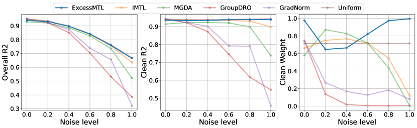
Figure 9: Results on the SARCOS dataset (noise in the first two joints). The left figure considers all 7 tasks, while the other two considers all tasks except the first two tasks. The right figure is the combined weights of all clean tasks (around 0.71 for uniform scalarization). ExcessMTL consistently maintains its performance, significantly outperforming other adaptive methods in face of label noise.

SARCOS [Vijayakumar and Schaal, 2000] presents an inverse dynamics problem for a robot arm with seven degrees of freedom. The task is to perform multi-target regression that uses 21 attributes (7 joint positions, 7 joint velocities, 7 joint accelerations) to predict the corresponding 7 joint torques. The noise is injected into the first two joint torques.

The results on SARCOS is presented in Figure 9. In the face of increasing label noise, all adaptive weighting algorithms except ExcessMTL exhibit a trend of assigning increasing weights to the noisy tasks. This behavior leads to a decline in performance on clean tasks. ExcessMTL demonstrates resilience to label noise, consistently maintaining its performance. Here, a similar pattern to MultiMNIST can be observed that uniform scalarization performs well. However, we want to emphasize again that the performance of uniform scalarization varies across all datasets, and it is not able to produce consistent results universally. In contrast, ExcessMTL demonstrates consistency across diverse datasets, reinforcing its robustness and effectiveness as a reliable solution in noisy environments.

References

• Amari (1998) Shun-ichi Amari. Natural gradient works efficiently in learning. Neural Computation, 10:251–276, 1998.
• Badrinarayanan et al. (2017) Vijay Badrinarayanan, Alex Kendall, and Roberto Cipolla. Segnet: A deep convolutional encoder-decoder architecture for image segmentation. IEEE transactions on pattern analysis and machine intelligence, 39(12):2481–2495, 2017.
• Burgert et al. (2022) Tom Burgert, Mahdyar Ravanbakhsh, and Begum Demir. On the effects of different types of label noise in multi-label remote sensing image classification. IEEE Transactions on Geoscience and Remote Sensing, 60:1–13, 2022. doi:10.1109/tgrs.2022.3226371.
• Caruana (1997) Rich Caruana. Multitask learning. Machine learning, 28:41–75, 1997.
• Chen et al. (2018) Zhao Chen, Vijay Badrinarayanan, Chen-Yu Lee, and Andrew Rabinovich. Gradnorm: Gradient normalization for adaptive loss balancing in deep multitask networks. In International conference on machine learning, pages 794–803. PMLR, 2018.
• Chen et al. (2020) Zhao Chen, Jiquan Ngiam, Yanping Huang, Thang Luong, Henrik Kretzschmar, Yuning Chai, and Dragomir Anguelov. Just pick a sign: Optimizing deep multitask models with gradient sign dropout. Advances in Neural Information Processing Systems, 33:2039–2050, 2020.
• Dai et al. (2016) Jifeng Dai, Kaiming He, and Jian Sun. Instance-aware semantic segmentation via multi-task network cascades. In Proceedings of the IEEE conference on computer vision and pattern recognition, pages 3150–3158, 2016.
• Désidéri (2012) Jean-Antoine Désidéri. Multiple-gradient descent algorithm (mgda) for multiobjective optimization. Comptes Rendus Mathematique, 350(5-6):313–318, 2012.
• Drori and Shamir (2020) Yoel Drori and Ohad Shamir. The complexity of finding stationary points with stochastic gradient descent. In International Conference on Machine Learning, pages 2658–2667, 2020.
• Duchi et al. (2011) John Duchi, Elad Hazan, and Yoram Singer. Adaptive subgradient methods for online learning and stochastic optimization. Journal of machine learning research, 12(7), 2011.
• Fliege and Svaiter (2000) Jörg Fliege and Benar Fux Svaiter. Steepest descent methods for multicriteria optimization. Mathematical Methods of Operations Research, 51(3):479–494, 2000.
• Guo et al. (2018) Michelle Guo, Albert Haque, De-An Huang, Serena Yeung, and Li Fei-Fei. Dynamic task prioritization for multitask learning. In Proceedings of the European conference on computer vision (ECCV), pages 270–287, 2018.
• Hazan et al. (2016) Elad Hazan et al. Introduction to online convex optimization. Foundations and Trends® in Optimization, 2(3-4):157–325, 2016.
• He et al. (2016) Kaiming He, Xiangyu Zhang, Shaoqing Ren, and Jian Sun. Deep residual learning for image recognition. In Proceedings of the IEEE conference on computer vision and pattern recognition, pages 770–778, 2016.
• Hsieh and Tseng (2021) Ming-En Hsieh and Vincent Tseng. Boosting multi-task learning through combination of task labels - with applications in ecg phenotyping. Proceedings of the AAAI Conference on Artificial Intelligence, 35(9):7771–7779, May 2021.
• Hu et al. (2020) Wei Hu, Zhiyuan Li, and Dingli Yu. Simple and effective regularization methods for training on noisily labeled data with generalization guarantee. In International Conference on Learning Representations, 2020.
• Hu et al. (2023) Yuzheng Hu, Ruicheng Xian, Qilong Wu, Qiuling Fan, Lang Yin, and Han Zhao. Revisiting scalarization in multi-task learning: A theoretical perspective. Advances in Neural Information Processing Systems, 2023.
• Kendall et al. (2018) Alex Kendall, Yarin Gal, and Roberto Cipolla. Multi-task learning using uncertainty to weigh losses for scene geometry and semantics. In Proceedings of the IEEE conference on computer vision and pattern recognition, pages 7482–7491, 2018.
• Kim et al. (2019) Youngdong Kim, Junho Yim, Juseung Yun, and Junmo Kim. Nlnl: Negative learning for noisy labels. In Proceedings of the IEEE/CVF international conference on computer vision, pages 101–110, 2019.
• Kingma and Ba (2015) Diederik P. Kingma and Jimmy Ba. Adam: A method for stochastic optimization. In Yoshua Bengio and Yann LeCun, editors, 3rd International Conference on Learning Representations, ICLR 2015, San Diego, CA, USA, May 7-9, 2015, Conference Track Proceedings, 2015.
• Kivinen and Warmuth (1997) Jyrki Kivinen and Manfred K Warmuth. Exponentiated gradient versus gradient descent for linear predictors. information and computation, 132(1):1–63, 1997.
• Lin and Zhang (2023) Baijiong Lin and Yu Zhang. LibMTL: A Python library for multi-task learning. Journal of Machine Learning Research, 24(209):1–7, 2023.
• Lin et al. (2022) Baijiong Lin, Feiyang Ye, Yu Zhang, and Ivor Wai-Hung Tsang. Reasonable effectiveness of random weighting: A litmus test for multi-task learning. Transactions on Machine Learning Research, 2022.
• Liu et al. (2021a) Bo Liu, Xingchao Liu, Xiaojie Jin, Peter Stone, and Qiang Liu. Conflict-averse gradient descent for multi-task learning. Advances in Neural Information Processing Systems, 34:18878–18890, 2021a.
• Liu et al. (2021b) Evan Z Liu, Behzad Haghgoo, Annie S Chen, Aditi Raghunathan, Pang Wei Koh, Shiori Sagawa, Percy Liang, and Chelsea Finn. Just train twice: Improving group robustness without training group information. In Marina Meila and Tong Zhang, editors, Proceedings of the 38th International Conference on Machine Learning, volume 139 of Proceedings of Machine Learning Research, pages 6781–6792. PMLR, 18–24 Jul 2021b.
• Liu et al. (2021c) Liyang Liu, Yi Li, Zhanghui Kuang, Jing-Hao Xue, Yimin Chen, Wenming Yang, Qingmin Liao, and Wayne Zhang. Towards impartial multi-task learning. In International Conference on Learning Representations, 2021c.
• Liu et al. (2019) Shikun Liu, Edward Johns, and Andrew J Davison. End-to-end multi-task learning with attention. In Proceedings of the IEEE/CVF conference on computer vision and pattern recognition, pages 1871–1880, 2019.
• Michel et al. (2021) Paul Michel, Sebastian Ruder, and Dani Yogatama. Balancing average and worst-case accuracy in multitask learning. arXiv preprint arXiv:2110.05838, 2021.
• Mukai (1980) Hiro Mukai. Algorithms for multicriterion optimization. IEEE Transactions on Automatic Control, 25(2):177–186, 1980. doi:10.1109/TAC.1980.1102298.
• Navon et al. (2022) Aviv Navon, Aviv Shamsian, Idan Achituve, Haggai Maron, Kenji Kawaguchi, Gal Chechik, and Ethan Fetaya. Multi-task learning as a bargaining game. Proceedings of Machine Learning Research, 162:16428–16446, 2022.
• Nemirovski et al. (2009) Arkadi Nemirovski, Anatoli Juditsky, Guanghui Lan, and Alexander Shapiro. Robust stochastic approximation approach to stochastic programming. SIAM Journal on optimization, 19(4):1574–1609, 2009.
• Nemirovskij and Yudin (1983) Arkadij Semenovič Nemirovskij and David Borisovich Yudin. Problem complexity and method efficiency in optimization. 1983.
• Piratla et al. (2021) Vihari Piratla, Praneeth Netrapalli, and Sunita Sarawagi. Focus on the common good: Group distributional robustness follows. In International Conference on Learning Representations, 2021.
• Sabour et al. (2017) Sara Sabour, Nicholas Frosst, and Geoffrey E Hinton. Dynamic routing between capsules. Advances in neural information processing systems, 30, 2017.
• Sagawa et al. (2020) Shiori Sagawa, Pang Wei Koh, Tatsunori B Hashimoto, and Percy Liang. Distributionally robust neural networks. In International Conference on Learning Representations, 2020.
• Sener and Koltun (2018) Ozan Sener and Vladlen Koltun. Multi-task learning as multi-objective optimization. Advances in neural information processing systems, 31, 2018.
• Shrivastava et al. (2016) Abhinav Shrivastava, Abhinav Kumar Gupta, and Ross B. Girshick. Training region-based object detectors with online hard example mining. 2016 IEEE Conference on Computer Vision and Pattern Recognition (CVPR), pages 761–769, 2016.
• Silberman et al. (2012) Nathan Silberman, Derek Hoiem, Pushmeet Kohli, and Rob Fergus. Indoor segmentation and support inference from rgbd images. ECCV (5), 7576:746–760, 2012.
• Venkateswara et al. (2017) Hemanth Venkateswara, Jose Eusebio, Shayok Chakraborty, and Sethuraman Panchanathan. Deep hashing network for unsupervised domain adaptation. In Proceedings of the IEEE Conference on Computer Vision and Pattern Recognition, pages 5018–5027, 2017.
• Vijayakumar and Schaal (2000) Sethu Vijayakumar and Stefan Schaal. Locally weighted projection regression: An o (n) algorithm for incremental real time learning in high dimensional space. In Proceedings of the seventeenth international conference on machine learning (ICML 2000), volume 1, pages 288–293. Morgan Kaufmann, 2000.
• Xue et al. (2019) Jiabin Xue, Jiqing Han, Tieran Zheng, Jiaxing Guo, and Boyong Wu. Hard sample mining for the improved retraining of automatic speech recognition, 2019.
• Ye et al. (2021) Feiyang Ye, Baijiong Lin, Zhixiong Yue, Pengxin Guo, Qiao Xiao, and Yu Zhang. Multi-objective meta learning. In A. Beygelzimer, Y. Dauphin, P. Liang, and J. Wortman Vaughan, editors, Advances in Neural Information Processing Systems, 2021. URL https://openreview.net/forum?id=wKf9iSu_TEm.
• Yu et al. (2020) Tianhe Yu, Saurabh Kumar, Abhishek Gupta, Sergey Levine, Karol Hausman, and Chelsea Finn. Gradient surgery for multi-task learning. Advances in Neural Information Processing Systems, 33:5824–5836, 2020.
• Yuan et al. (2017) Yuhui Yuan, Kuiyuan Yang, and Chao Zhang. Hard-aware deeply cascaded embedding. In Proceedings of the IEEE International Conference on Computer Vision (ICCV), Oct 2017.
• Zhou et al. (2022) Shiji Zhou, Wenpeng Zhang, Jiyan Jiang, Wenliang Zhong, Jinjie Gu, and Wenwu Zhu. On the convergence of stochastic multi-objective gradient manipulation and beyond. Advances in Neural Information Processing Systems, 35:38103–38115, 2022.