Understanding Time Series Anomaly State Detection through One-Class Classification

Abstract

For a long time, research on time series anomaly detection has mainly focused on finding outliers within a given time series. Admittedly, this is consistent with some practical problems, but in other practical application scenarios, people are concerned about: assuming a standard time series is given, how to judge whether another test time series deviates from the standard time series, which is more similar to the problem discussed in one-class classification (OCC). Therefore, in this article, we try to re-understand and define the time series anomaly detection problem through OCC, which we call ’time series anomaly state detection problem’. We first use stochastic processes and hypothesis testing to strictly define the ’time series anomaly state detection problem’, and its corresponding anomalies. Then, we use the time series classification dataset to construct an artificial dataset corresponding to the problem. We compile 38 anomaly detection algorithms and correct some of the algorithms to adapt to handle this problem. Finally, through a large number of experiments, we fairly compare the actual performance of various time series anomaly detection algorithms, providing insights and directions for future research by researchers.

1 Introduction

Time series anomaly detection emerges as an indispensable technique across diverse sectors, playing a pivotal role in identifying deviations from established normative patterns. This method finds extensive application in areas such as financial markets, network security, industrial process monitoring, and more (Hilal et al., 2022; Kaur et al., 2017; Park et al., 2020; Fahim & Sillitti, 2019). Leveraging the wealth of data produced by these industries for real-time surveillance of anomalous events can significantly mitigate potential losses in human, environment, and energy resources (Fernando et al., 2021; Russo et al., 2020; Jesus et al., 2021; Himeur et al., 2021).

Given the wide application and importance of time series anomaly detection, it has received widespread academic and industrial attention and developed rapidly from six decades ago (Fox, 1972; Page, 1957; Tsay, 1988; Tukey et al., 1977; Chang et al., 1988). Besides, as machine learning becomes more popular in various data science tasks, researchers have begun to explore the use of machine learning methods in these tasks to detect anomalies in time series data. For example, classification algorithms such as support vector machines (Hearst et al., 1998) and time series forecasting algorithms such as ARIMA (Box & Jenkins, 1976) have proven useful in identifying anomalies in time series data. In recent years, with the rise of neural network technology, a large number of emerging anomaly detection algorithms are based on neural network architecture, which is roughly applied in three aspects: feature extraction, learning feature representations of normality, and end-to-end anomaly score learning (Pang et al., 2021).

Most of the articles on anomaly detection algorithms mentioned above are concerned with identifying individual observations that are significantly deviated from other observations in the dataset, that is, outliers, and often called ‘Outlier Detection’, ‘Outlier Analysis’ or ‘Anomalous Pattern Detection’ (Das et al., 2008; Kim & Park, 2020), which is an important task in time series anomaly detection and can be considered as a function $\phi_{\text{binary}}$ (Braei & Wagner, 2020),

$$\phi_{\text{binary}}:\mathbb{R}^{\omega}\rightarrow\{\text{normal, anomaly}\}$$ (1)

$$\phi_{\text{binary}}(x)\mapsto\begin{cases}\text{anomaly, }&\text{ if }\phi_{\text{score }}(x)=\gamma>\delta\\ \text{normal, }&\text{ otherwise }\end{cases}$$

where $\phi_{\text{score}}$ is an anomaly detection algorithm, $\gamma$ is the anomaly score, $\delta\in\mathbb{R}$ is the threshold to determine whether a point is anomaly, $x\in X\subseteq\mathbb{R}^{\omega}$, $X$ is the dataset, and $\omega$ is the width of the sliding window. The objective of $\phi_{\text{binary}}$ is to detect rare data points that deviate remarkably from the general distribution of the dataset (Braei & Wagner, 2020).

However, in addition to the ‘Outlier Detection’ discussed above, there’s another kind that’s widely used in industrial manufacturing but hasn’t received much attention, which can be briefly described as follows: given a standard time series, how to determine if another test time series deviates from this standard time series? Here we temporarily call this problem the ‘Time Series Anomaly State Detection Problem’. It’s a way of looking at time series anomaly detection from a one-class classification perspective.

The ‘time series anomaly state detection’ has a wide range of practical applications. For example, in the field of mechanical equipment inspection, it is used to systematically monitor and evaluate the operating status of mechanical systems to ensure their optimal operation. Similarly, within the scope of power system monitoring, it plays a key role in the identification and analysis of grid anomalies, including harmonic distortion, voltage fluctuations and frequency irregularities, which indicates potential system issues or instability within the grid infrastructure. Furthermore, in the domain of wireless communications, it is pivotal for the surveillance of signal interference and anomalies in signal strength, a key aspect in ensuring the reliability of communication networks.

Despite its substantial utility in industrial applications, ‘time series anomaly state detection problem’ has not yet captured significant attention within the computer science community. This is reflected in the relatively limited research and literature dedicated to the development of specialized algorithms for addressing this challenge. Therefore, a purpose of our paper is to introduce the problem to the field of computer science and stimulate discourse within the research community. This effort will be achieved through careful elaboration and precise definition of the problem and proposing a comprehensive framework for solving it. The main contributions of our study can be summarized as follows:

• Introduction to a conceptual framework: Our study introduces a novel conceptual framework by rigorously defining the ‘time series anomaly state detection problem’ as well as its corresponding anomaly with mathematical tools, and then propose an implementation framework that can be carried out concretely.

• Synthetic dataset construction: Considering that the definition of this problem is different from traditional outlier detection, a general dataset cannot be used. Therefore, this paper proposes a dataset construction method: generate data from a time series classification dataset, and applies it to experimental analysis.

• Empirical Evaluation and Comparative Analysis: Finally, our study culminates in an extensive empirical evaluation, in which the performance of 38 algorithms modified for our task is unbiasedly compared within our established framework. This comparative analysis sheds light on the relative strengths and weaknesses of different algorithms, as well as their time efficiency and stability, thereby providing valuable insights for future research and applications in this area.

2 Related Work

There are various algorithms for detecting anomalies in time series, which can be roughly divided into four categories based on their working mechanisms, namely, forecast-based, reconstitution-based, statistical-model-based, and proximity-based algorithms.

Forecast-based algorithms refer to ones, wherein predictive models are trained to anticipate future values first, and subsequently, identify the anomaly by assessing the disparity between the predicted values and the actual observed values. Its representative algorithms include polynomial-based models, LinearRegreesion(LR), and neural-networks-based models, fully connected neural networks (FCNN) (Back & Tsoi, 1991), convolutional neural networks (CNN) (Munir et al., 2018), recurrent neural network (RNN) (Connor et al., 1994), gated recurrent unit (GRU) (Chung et al., 2014), and long short-term memory (LSTM) (Hundman et al., 2018; Hochreiter & Schmidhuber, 1997).

Reconstitution-based algorithms aim to learn a model that captures the latent structure of the given time series data and generate synthetic reconstitution, and then discriminate the anomaly by reconstitution performance under assumption that outliers cannot be efficiently reconstructed from the low-dimensional mapping space. Reconstitution-based algorithms can be mainly divided into two categories: low-dimensional feature space reconstitution, including Kernel Principal Component Analysis (KPCA) (Hoffmann, 2007), Auto-Encoder (AE) (Sakurada & Yairi, 2014), Variational Auto-Encoder (VAE) (Kingma & Welling, 2013), and Transformer, and adversarial generation models, including Time Series Anomaly Detection with Generative Adversarial Networks (TanoGan) (Bashar & Nayak, 2020) and Time Series Anomaly Detection Using Generative Adversarial Networks (TadGan) (Geiger et al., 2020).

Statistical-model-based algorithms assume that data is generated by a certain statistical distribution, and use statistical models to perform hypothesis testing to determine which data does not meet the model assumptions, thereby detecting outliers. Generally, it can be divided into two categories, namely, methods based on empirical distribution functions, including Copula-Based Outlier Detection (COPOD) (Li et al., 2020), Empirical Cumulative Distribution-Based Outlier Detection (ECOD) (Li et al., 2022), Histogram-based outlier detection (HBOS) (Birgé & Rozenholc, 2006), Lightweight on-line detector of anomalies (LODA) (Pevnỳ, 2016), and methods based on theoretical distribution functions, including Gaussian Mixture Models (GMMs) (Aggarwal & Sathe, 2015), Kernel density estimation (KDE) (Latecki et al., 2007), Mean Absolute Differences (MAD) (Iglewicz & Hoaglin, 1993) Algorithm, Outlier Detection with Minimum Covariance Determinant (MCD) (Rousseeuw & Driessen, 1999).

Proximity-based algorithms for anomaly detection are techniques that rely on using various distance measures to quantify similarity or proximity between data points, including density, distance, angle and dividing hyperspace, and then identify anomalies, under the assumption that distribution of abnormal points is different from that of normal points, causing the similarity or proximity low. Density-based algorithms includes Cluster-Based Local Outlier Factor (CBLOF) (He et al., 2003), Connectivity-Based Outlier Factor (COF) (Tang et al., 2002), Local Outlier Factor (LOF) (Breunig et al., 2000), Quasi-Monte Carlo Discrepancy outlier detection (QMCD) (Fang & Ma, 2001); Distance-based methods includes Cook’s distance outlier detection (CD) (Cook, 1977), Isolation-based anomaly detection using nearest-neighbor ensembles (INNE) (Bandaragoda et al., 2018), K-means outlier detector (Kmeans) (Chawla & Gionis, 2013), K-Nearest Neighbors (KNN) (Ramaswamy et al., 2000), Outlier detection based on Sampling (SP) (Sugiyama & Borgwardt, 2013), Principal Component Analysis algorithm (PCA) (Shyu et al., 2003), Subspace Outlier Detection (SOD) (Kriegel et al., 2009), Stochastic outlier selection (SOS) (Janssens et al., 2012); Angle-based methods include Angle-based outlier detection (ABOD) (Kriegel et al., 2008); Dividing-hyperplane-based methods includes Deep One-Class Classification for outlier detection (DeepSVDD) (Ruff et al., 2018), Isolation forest (IForest) (Liu et al., 2008), One-class SVM (OCSVM) (Schölkopf et al., 2001), One-Classification using Support Vector Data Description (SVDD) (Tax & Duin, 2004).

However, algorithms mentioned above mainly focus on problems related to outlier detection. Therefore, we hope to provide a basic and complete paradigm for solving ‘time series anomaly state detection problem’ by strictly defining the problem and conducting detailed experimental analysis. Our goal is not only to solve the problem, but also strive to build a solid academic foundation and aim to provide a pioneering framework that guides and enhances future research efforts in this specialized area.

3 Time Series Anomaly State Detection

3.1 Mathematical Definition Of The Problem

Stochastic Process: Suppose $E$ is a random experiment and the sample space is $S=\{e\}$, if for each sample point $e\in S$, there always exists a time function $X(t,e)$ and $t\in T$ corresponds to it. Then in this way, the family of time $t$ functions $\{X(t,e),t\in T\}$ obtained for all $e\in S$ is called a stochastic process, abbreviated as $\{X(t),t\in T\}$. Each function in the family is called a sample function of this Stochastic process. $T$ is the variation range of parameter $t$, which is called parameter set.

Time Series: A time series $\{X(t),t\in\mathbb{N}\}$ is defined as a stochastic process with discrete time points. $x(t)$ represent the observed value of $X(t)$, and call $\{x(t),t\in\mathbb{N}\}$ an orbit of $\{X(t),t\in\mathbb{N}\}$.

Problem (Time Series Anomaly State Detection through One-Class Classification): Given a standard time series dataset of inliers $\mathcal{D}=\{\tilde{x}_{j}(t),t\in[\tilde{N}_{j}]\}_{j=1}^{m_{0}}$, containing $m_{0}$ independently and identically distributed (i.i.d) orbits $\{\tilde{x}_{j}(t)\}_{t=1}^{\tilde{N}_{j}},\tilde{x}_{j}(t)\in\mathbb{R}^{d_{0}}$ of a standard stochastic process $\{X_{0}(t),t\in\mathbb{N}\}$ (a set of standard stochastic process $\{X_{p}(t),t\in\mathbb{N}\}_{p=1}^{n_{p}}$), and an unseen test time series dataset $\mathcal{U}=\{\hat{x}_{j}(t),t\in[\hat{N}_{j}]\}_{j=1}^{m_{1}},\hat{x}_{j}(t)\in\mathbb{R}^{d_{0}}$ and its segment subset $\mathcal{U}_{\mathcal{S}}=\{S_{j}^{k}\triangleq\{\hat{x}_{j}(t),t\in[r_{k},s_{k}]\}\}_{j\in[1,m_{1}],k\in\mathbb{N}}$, where $S_{j}^{k}$ is segment intercepted from the test time series orbit, the goal of time series anomaly detection from OCC problem is to identify the outlier segment set $\mathcal{O}=\{S_{j}^{k}\subset\{\hat{x}_{j}(t),t\in[\hat{N}_{j}]\}\in\mathcal{U}:S_{j}^{k}\nsim\{X_{0}(t),t\in\mathbb{N}\}\}$.

In order to deal with this time series anomaly state detection problem, we can consider the following mathematical framework. First, employ a pre-processing function $\mathcal{P}$ to extract time information features $\mathcal{F}_{standard}\triangleq\mathcal{P}(\mathcal{D})$ and $\mathcal{F}_{test}\triangleq\mathcal{P}(\mathcal{U_{\mathcal{S}}})$. And then, employ the detection algorithm $\mathcal{M}$ and standard pre-processed dataset $\mathcal{F}_{standard}$ to learn a anomaly score function $A_{\mathcal{M}}(\cdot)$. Next, use the learned anomaly score function $A_{\mathcal{M}}(\cdot)$ to infer an anomaly score $A_{\mathcal{M}}(\mathcal{P}(S_{j}^{k}))$ to assess whether $S_{j}^{k}$ is an outlier. Generally, it is assumed that the larger the anomaly score $A_{\mathcal{M}}(\mathcal{P}(S_{j}^{k}))$, the more likely the corresponding $S_{j}^{k}$ is an outlier. Therefore, the decision set (detected outlier segment set) is selected as: $\hat{\mathcal{O}}_{\mathcal{M}}=\{S_{j}^{k}\subset\{\hat{x}_{j}(t),t\in[\hat{N}_{j}]\}\in\mathcal{U}:A_{\mathcal{M}}(\mathcal{P}(S_{j}^{k}))\geq L_{\mathcal{M}}\}$, where $L_{\mathcal{M}}$ is a threshold associated with detector $\mathcal{M}$. Denote the subset of $\mathcal{U}_{\mathcal{S}}$ containing all inliers as $\mathcal{O}^{c}=\{S_{j}^{k}\subset\{\hat{x}_{j}(t),t\in[\hat{N}_{j}]\}\in\mathcal{U}:S_{j}^{k}\sim\{X_{0}(t),t\in\mathbb{N}\}\}$, and $\mathcal{O}\cup\mathcal{O}^{c}=\mathcal{U}$.

Taking a multiple testing perspective, the null hypothesis is that a new time series segment is an inlier, while the alternative asserts that it is an outlier. That is, the time series anomaly state detection from one-class classification problem is translated into a multiple testing problem as follows,

$$\mathbb{H}_{0,(j,k)}:S_{j}^{k}\sim\{X_{0}(t),t\in\mathbb{N}\}\quad v.s.$$ (2)

$$\mathbb{H}_{1,(j,k)}:S_{j}^{k}\nsim\{X_{0}(t),t\in\mathbb{N}\}\ ,\ j=1,\dots,n,\ k\in\mathbb{N}$$

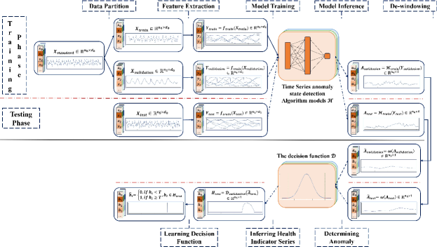
Figure 1: Overview of the implementation frame. The entire framework is divided into a training phase and a testing phase. The training phase is used to learn the characteristics of standard time series, while the testing phase is used to infer anomalies in the test time series.

3.2 Implementation framework of time series anomaly state detection

In the preceding subsection, we utilized knowledge of stochastic processes to define time series anomaly state detection and presented a mathematical framework for addressing it. However, this framework, while theoretically robust, is abstract and not applicable in practice. Therefore, in this subsection, we shift our focus to practical application, proposing a framework that can be implemented to solve this problem in real-world scenarios. Specifically, our implementation process are divided into two distinct phases: the training phase and the testing phase, as shown in Fig. 1.

In the training phase, as delineated in Fig. 1 and Algorithm 2 in Appendix A.1, the process primarily encompasses several key steps: data partition, feature extraction, model training, model inference, de-windowing and learning decision function. While, in the testing phase, also as outlined in Fig. 1 and Algorithm 3 in Appendix A.1, the procedure mainly includes: feature extraction, model inference, de-windowing, inferring health indicator series, and determining anomaly.

Based on the implementation framework proposed above, we further conduct an intuitive analysis and define the outliers under this framework in Appendix A.2.

4 Preparation for Experiments

4.1 Construction of Dataset

There are many open source anomaly detection data sets on the market, including open source nature data  (Lavin & Ahmad, 2015; Paparrizos et al., 2022b; Bhatnagar et al., 2021) and artificial ones  (Lavin & Ahmad, 2015; Han et al., 2022; Lai et al., 2021). However, they serve the task of outlier detection, where anomalies in these datasets are often departure points that deviate from the overall distribution within the time series, which cannot be applied to our task.

4.1.1 Basic guidelines for data construction

As we defined the task in Sec. 3.1, we consider a segment as an outlier if it does not appear in standard time series. Therefore, an intuitive idea is to first find a suitable time series baseline, which follows a set of certain given stochastic process, and then divide it into standard time series and pre-test time series, where outliers are injected into the pre-test time series to form test time series. And, we believe that three basic requirements must be met: (i) The baseline has a certain periodicity. This ensures that the normal part of the “test time series” should have appeared in the training data; if there is no periodicity at all, then the “test time series” is likely to be abnormal at all. (ii) There is a certain amount of ”noise”. We hope that each period has a certain similarity, but not exactly the same, which is more consistent with the real working conditions; (iii) There is more effective information than ”noise”. That is, we hope that the baseline has a high signal-to-noise ratio.

4.1.2 Build datasets from categorical time series data

Based on the intuitive idea and requirements in the previous subsection, using the time series classification dataset to construct an time series anomaly state detection dataset seems to be suitable, for in time series classification datasets, data belonging to one category tends to be relatively close, while there are certain differences between data in different categories. Therefore, if we use a certain category in the classification datasets as the baseline and then appropriately insert another category into the test data as anomaly data, then we could create time series anomaly state detection dataset that meets our requirements in previous subsection. To ensure the quality of the constructed dataset, we hope that the normal part of the test time series data is close to the standard time series data, while the abnormal part has a certain distance from the standard time series data. Finally, to satisfy the discussion above demands, we construct the artificial dataset as Algorithm 1. In order to ensure the quality of the dataset, we use algorithms and data to check each other: if the AUC-ROC of the results of all algorithms on a dataset is below 0.8, then we will remove this artificial data from the artificial dataset.

Algorithm 1 Build datasets from categorical time series data

0:  The data from a given classification dataset $\{(X_{i},y_{i})\}_{i=1}^{N},X_{i}\in\mathbb{R}^{m},y\in\mathbb{R}$, and the shape-based distance (sbd) distance $d(x,y)$.

1:  Pick out the $k$-th type of data $\{(X_{i},y_{i})\}_{y_{i}=k}$

2:  Perform k-means clustering with sbd on $\{(X_{i},y_{i})\}_{y_{i}=k}$ to ensure that similar data can be found even in one category and ensure the consistency of the baseline.

3:  Select the most concentrated category $\{(X_{i},y_{i})\}_{y_{i}=\hat{k}}$ in 2 as baseline and randomly shuffle it.

4:  Calculate the average distance $\{d(x_{i},y_{i})\}_{y_{i}\neq k}$ from each data in other categories to the baseline $\{(X_{i},y_{i})\}_{y_{i}=\hat{k}}$, respectively.

5:  Extract the first half of the baseline dataset $\{(X_{i},y_{i})\}_{y_{i}=\hat{k}}$, and sequentially concatenate these elements to construct the standard time series, denoted as $X_{standard}$. Subsequently, based on the average distance $\{d(x_{i},y_{i})\}_{y_{i}\neq k}$, incorporate suitable data from categories other than the $k$-th into the second half of $\{(X_{i},y_{i})\}_{y_{i}=\hat{k}}$ randomly. These are then sequentially concatenated to form the test time series, labeled as $X_{test}$.

4.2 The Time Series Anomaly State Detection Algorithms Under One-Class Classification

In this paper, we look at time series anomaly state detection from the perspective of One-Class Classification, therefore, we have modified anomaly detection algorithms so that they can maintain the ability to handle traditional outlier detection tasks, while also being able to handle the time series anomaly state detection tasks we defined. We have compiled a comprehensive algorithm collection with 38 time series anomaly detection methods, which could be categorized into four types based on their working mechanisms, i.e., forecast-based algorithms, reconstitution-based algorithms, statistical-model-based algorithms, and proximity-based algorithms. For the introduction of these algorithms, we have described them in Sec. 2, and provide more information about them in Appendix B.1.

Table 1: Average value of eight representative accuracy evaluation measures for all the thirty-eight algorithms.

Algorithms	Precision	Recall	F1	Range-F1	AUC-ROC	AUC-PR	VUS-ROC	VUS-PR
ABOD	0.183	0.200	0.158	0.174	0.797	0.775	0.664	0.650
AE	0.743	0.729	0.613	0.655	0.907	0.802	0.785	0.680
CBLOF	0.799	0.631	0.562	0.656	0.879	0.773	0.771	0.664
CD	0.378	0.197	0.165	0.253	0.596	0.583	0.514	0.510
CNN	0.739	0.690	0.567	0.633	0.876	0.741	0.757	0.629
COF	0.815	0.591	0.543	0.650	0.858	0.724	0.765	0.624
COPOD	0.412	0.220	0.207	0.297	0.678	0.425	0.572	0.359
DeepSVDD	0.754	0.807	0.644	0.680	0.913	0.764	0.816	0.677
ECOD	0.452	0.247	0.232	0.341	0.686	0.428	0.580	0.370
FCNN	0.813	0.696	0.596	0.663	0.881	0.753	0.776	0.653
GMM	0.683	0.672	0.553	0.614	0.861	0.684	0.751	0.588
GRU	0.581	0.579	0.463	0.508	0.822	0.628	0.696	0.524
HBOS	0.721	0.488	0.448	0.549	0.810	0.686	0.692	0.583
IForest	0.730	0.520	0.474	0.568	0.838	0.707	0.710	0.595
INNE	0.708	0.581	0.505	0.577	0.844	0.740	0.732	0.646
KDE	0.812	0.776	0.641	0.690	0.921	0.811	0.792	0.688
KMeans	0.818	0.689	0.614	0.685	0.895	0.803	0.795	0.700
KNN	0.798	0.799	0.686	0.719	0.949	0.857	0.847	0.749
KPCA	0.602	0.724	0.560	0.574	0.883	0.705	0.765	0.606
LinearRegression	0.450	0.459	0.352	0.403	0.746	0.501	0.645	0.422
LODA	0.693	0.466	0.395	0.510	0.785	0.640	0.664	0.565
LOF	0.750	0.873	0.713	0.701	0.953	0.851	0.865	0.762
LSTM	0.578	0.621	0.485	0.527	0.827	0.649	0.713	0.547
MAD	0.582	0.357	0.320	0.406	0.752	0.581	0.616	0.502
MCD	0.511	0.472	0.366	0.435	0.751	0.537	0.631	0.441
MSD	0.493	0.290	0.259	0.341	0.704	0.510	0.583	0.450
OCSVM	0.466	0.153	0.161	0.311	0.614	0.387	0.533	0.355
PCA	0.275	0.066	0.085	0.177	0.566	0.332	0.499	0.314
QMCD	0.053	0.443	0.074	0.074	0.654	0.663	0.598	0.595
RNN	0.600	0.636	0.507	0.554	0.841	0.667	0.729	0.571
Sampling	0.841	0.818	0.718	0.762	0.956	0.873	0.858	0.769
SOD	0.771	0.678	0.567	0.630	0.875	0.714	0.752	0.607
SOS	0.510	0.825	0.535	0.476	0.955	0.851	0.883	0.740
SVDD	0.642	0.421	0.362	0.491	0.757	0.567	0.640	0.513
TadGan	0.804	0.582	0.523	0.622	0.843	0.736	0.733	0.639
TanoGan	0.446	0.176	0.193	0.313	0.651	0.529	0.541	0.481
Transformer	0.675	0.510	0.441	0.519	0.806	0.620	0.685	0.531
VAE	0.691	0.559	0.481	0.541	0.831	0.692	0.698	0.576

4.3 Accuracy Evaluation Measures

Many accuracy evaluation measures have been proposed to quantitatively evaluate the detection performance of different anomaly detection algorithms and help select the optimal model through comparison. In this article, we will mainly focus on four threshold-based measures, Precision, Recall, F1-score, and Range F1-score (Tatbul et al., 2018), and four threshold-independent measures, the area under (AUC) the receiver operating characteristics curve (AUC-ROC) and the precision-recall curve (AUC-PR), and the volume under the surface (VUS) for the ROC surface (VUS-ROC) and PR surface (VUS-PR)  (Paparrizos et al., 2022a). Considering that threshold-independent measures are generally better than threshold-based ones in terms of robustness, separability and consistency (Paparrizos et al., 2022a), we will conduct more analyzes based on them in this article.

4.4 Methods to evaluate the difficulty of TSADBench dataset

In addition to accuracy evaluation measures, the quantification of the difficulty coefficient of the dataset should also be considered, which helps to conduct a more detailed evaluation of model performance. A comprehensive understanding of the properties of the dataset can not only enrich the comparative analysis of algorithms, such as robustness, but can also guide the selection and calibration of models in practical applications.

Previous articles have discussed several indicators to measure the difference in distribution of normal points and abnormal points, including Relative Contrast (RC) (He et al., 2012), Normalized clusteredness of abnormal points (NC) (Emmott et al., 2013), and Normalized adjacency of normal/abnormal cluster (NA) (Paparrizos et al., 2022b), which we elaborate on in Appendix B.2.

However, the three indicators RC, NC and NA are all constructed for traditional outlier analysis, and are not applicable to the dataset we constructed. Therefore, inspired by the previous work and combined with the characteristics of our task, we proposed the k-nearest-neighbors (knn) normalized clusteredeness (KNC) of abnormal points method to measure the difference between the distributions of normal points and abnormal points, and use it to evaluate the difficulty of the our dataset. Suppose that $s$ represents time series, $D(s_{i},s_{j})$ denote the SBD distance between two series $s_{i}$ and $s_{j}$, $S$ is the whole set, $\mathcal{S}_{std}$ denotes the set of standard sequences, $\mathcal{S}_{nor}$ and $\mathcal{S}_{abn}$ denotes the set of normal and anomalous sequences in test sequences, and $D^{k}_{mean}(x,\mathcal{S})=\frac{1}{k}\sum_{s_{i}\in\text{knn to x},s_{i}\in\mathcal{S}}D(x,s_{i})$ is the mean SBD distance between time series $x$ and its k-nearest-neighbors in the set $\mathcal{S}$, then we define KNC as the ratio of the average k-nearest-neighbor SBD distance between the anomalous sequences and standard set to that between the normal sequences and standard set,

$$KN_{c}=\frac{\mathbb{E}_{s\in S_{\text{ano}}}\left[D^{k}_{mean}(s,\mathcal{S}_{std})\right]}{\mathbb{E}_{s\in S_{\text{nor}}}\left[D^{k}_{mean}(s,\mathcal{S}_{std})\right]}$$ (3)

The K-nearest-neighbor here is critical, because we do not require the data in the test data set to be close to all the data in the standard data set, but only require that there is data in the standard data set that is close to it.

5 Experiments

5.1 Experiments setup

5.1.1 Feature Extraction

1) Feature extraction: For each dataset, we first normalize the data between $[0,1]$. Then we set the window lengths to 32, 64, 128, 256, the length based on (Imani & Keogh, 2021), the length based on Auto-correlation Function, and the length based on Fourier transform, respectively, with stride equals to 1 .

2) Algorithms: Here, we have implemented all 38 algorithms mentioned in Sec. 4.2, and the key parameters of each algorithm have been tried within the appropriate range.

3) De-windowing function $\omega$: Given the original time series $X\in\mathbb{R}^{n_{x}\times d_{x}}$ and the corresponding anomaly score $A\in\mathbb{R}^{n_{y}\times 1}$, then modified anomaly score $\hat{A}=w(A)=(\hat{a}_{1},\hat{a}_{2},\dots,\hat{a}_{n_{x}})\in\mathbb{R}^{n_{x}\times 1}$ is defined as follows:

For a given $i\in[n_{x}]$, assume that $\mathcal{S}_{i}$ is the serial number set of $A$ which contains the information of $x_{i}$, then we have $\hat{a}_{i}=\frac{1}{|\mathcal{S}_{i}|}\sum_{j\in\mathcal{S}_{i}}a_{j}$.

4) Decision function $\mathcal{D}$ and decision threshold $T$: Given the validation modified anomaly score $\hat{A}_{v}$, the decision function $\mathcal{D}$ is modified by the integral cumulative distribution function of the standard normal distribution and defined as follows. Let $\mu$ be the mean of $\hat{A}_{v}$, and $\sigma$ be the variance of $\hat{A}_{v}$, then $\mathcal{D}(\hat{a})=\max((\operatorname{erf}((\hat{a}-\mu-\sigma)/(\sqrt{2}\sigma))-0.5)*2,0),\ \operatorname{erf}(x)=\frac{2}{\sqrt{\pi}}\int_{0}^{x}e^{-t^{2}}dt$, with the decision threshold $T=1-(1-\operatorname{erf}(2/\sqrt{2}))/2$

The decision function $\mathcal{D}$ here is essentially calculating the significance level $\alpha$ of $\hat{a}$ under a given modified test anomaly score $\hat{A}_{t}$. The transformation operations consider that only when $\hat{a}$ and $\mu$ reaches a certain distance, then $\hat{a}$ begin to be viewed as an outlier. We hope that when $\mathcal{D}(\hat{a})>0$, it means that an abnormality may occur. The decision threshold $T$ is chosen as $2\sigma$ because when calculating the decision function $\mathcal{D}$, $\hat{a}$ has already been subtracted by a $\sigma$.

5.2 Overall experimental results

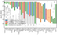
(a) Algorithms performance based on AUC-ROC

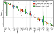
(b) Algorithms ranks under accuracy evaluation measures

Figure 2: The performance of different algorithms on all 38 algorithms, sorted in descending order based on median. In (a), the vertical axis represents AUC-ROC, and in (b), the vertical axis represents the ranks of the chosen evaluation measures. Colors indicate the type of anomaly detection algorithms.

We first conduct 38 algorithms on the artificial dataset generated by categorical dataset, which contains about 369 time series with labeled anomalies. Table 1 presents the average value of eight representative accuracy evaluation measures (i.e., precision, recall, f1-score, range-f1-score, auc-roc, auc-pr, vus-roc, vus-pr) for all the thirty-eight algorithms across the dataset. Fig. 2(a) presents the average AUC-ROC across the entire datasets and algorithms. The results of other accuracy evaluation measures could be found in the Appendix C.1. Furthermore, we calculate the ranks of all algorithms under the eight representative accuracy evaluation measures across the dataset, and draw a boxplot of the ranks of each algorithm under these measures, as shown in Fig. 2(b). From this initial inspection, three methods seem to perform well: Sampling, LOF and KNN. According to the classification of anomaly detection algorithms, the best-performing forecast-based algorithm is FCNN, the best-performing reconstitution-based algorithm is the FCNN algorithm, the best-performing statistical-model-based algorithm is the KNN algorithm, and the best-performing proximity-based algorithm is the Sampling algorithm. Through this ranking, we have initially observed two very interesting phenomena: (1) In fact, the algorithms with the best results are not algorithms based on neural networks, but some traditional distance-based algorithms; (2) In prediction-based algorithms with neural networks, the best performing one is the simplest FCNN, rather than ones with special structures.

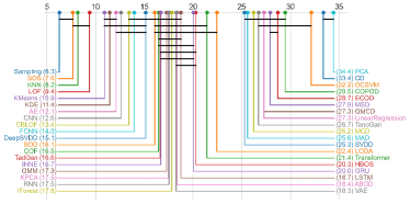
Figure 3: Critical difference of 38 algorithms based on AUC-ROC

To better understand the ranks of the algorithms, we employed a Critical Difference (CD) diagram to illustrate and evaluate the comparative performance of various anomaly detection algorithms across the entire datasets. The CD diagram reveals the relative performance of the algorithms and their statistical significance of differences. Algorithms are arrayed according to their average ranks across all datasets, with the significance of performance differences ascertained through the Friedman test followed by Wilcoxon signed-rank test [113]. From the critical difference diagram in Fig. 3 of AUC-ROC, we observe that the ’Sampling’ algorithm (with an average rank of 6.1) significantly outperforms the rest of the algorithoms significantly except ’SOS’ algorithm. This result is consistent with the results of each algorithm in Fig. 2(a). Critical difference graphs for more accuracy evaluation measures can be found in Appendix C.2.

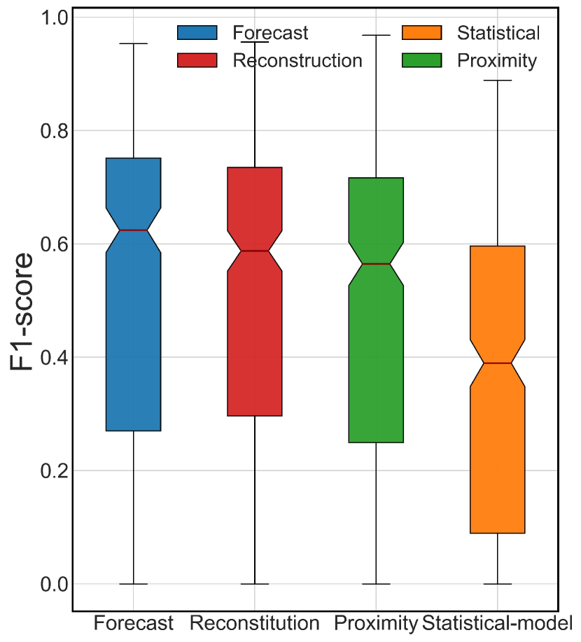
(a) F1-score

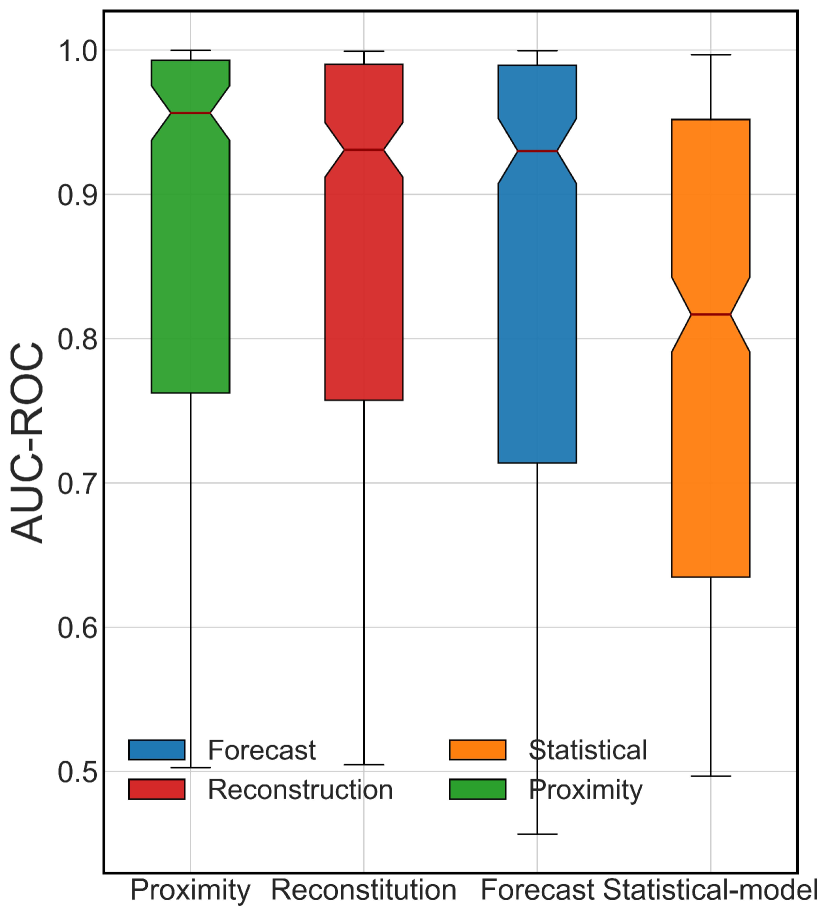
(b) AUC-ROC

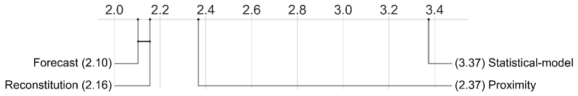
(c) Critical Difference under F1-score

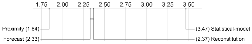
(d) Critical Difference under AUC-ROC

Figure 4: The performance of four types of anomaly detection algorithms under the AUC-ROC and F1 accuracy evaluation measures. (a,b) depict the performance of the four algorithms on the entire dataset in box-plots, while (c,d) further utilize CD diagram to reflect whether there are significant differences between them.

5.3 Comparison among four different based algorithms

Previously, we demonstrated the performance across different anomaly detection algorithms, whose results vary significantly. In this section, we will illustrate the analysis under the four types of algorithms , i.e., forecast-based algorithms, reconstitution-based algorithms, statistical-model-based algorithms, and proximity-based algorithms.

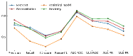
(a) Value of algorithms under eight evaluation measures

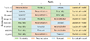
(b) Ranks of algorithms under eight evaluation measures

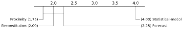
(c) Critical Difference of algorithms of the average ranks.

Figure 5: Performance of four kinds of anomaly detection algorithms under 8 different anomaly metrics. (a) depicts the specific values of four types of algorithms under different evaluation measures, (b) depicts the specific ranks between them, and (c) is concerned with whether there are significant differences between them.

First, we consider the overall situation of four types of algorithms under different accuracy evaluation measures. Specifically, for a given evaluation measure, we first consider the performance of four types of algorithms on each sub-data, take the median of each category of algorithms as the evaluation score for the data, and finally calculate the average scores of all sub-data, as the final score. We found that under F1-score, there is no significant difference between the reconstitution and forecast algorithms, which are all significantly better than proximity and statistical-model algorithms, as shown in Fig. 4(a,c). Under F1-score in Fig. 4(b,d), the proximity-based algorithm is significantly better than the other three algorithms. The results of more evaluation indicators can be found in Appendix XX.

Considering the difference in rankings under different evaluation measures, we further compared the results of the four types of algorithms under the eight representative evaluation measures, as shown in Fig. 5(a). As shown in Fig. 5(b), proximity-based algorithms achieve the best ranking under the eight evaluation measures, while statistical-model-based algorithms perform the worst. At the same time, in the CD diagram in Fig. 5(c), We can also find that proximity-based algorithms rank first with an average ranking of 1.75, followed by reconstruction-based algorithms with 2.00, prediction-based algorithms with 2.25, and statistical-model-based algorithms with 4.00.

5.4 Comparison of time required by algorithms

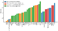
(a) Time spent by algorithms

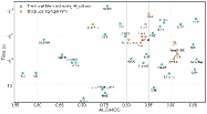
(b) AUC-ROC v.s. time

Figure 6: Comparison of time spent by different algorithms. In (a), the left side of red dotted line represents the traditional machine learning algorithms running on CPU, while the right side represents the deep learning algorithms running on GPU. (b) presents a comparison of AUC-ROC and runtime for different algorithms.

We also compared the time spent by each algorithm in processing the time series anomaly state detection problem. We randomly selected 3 sets of data from the entire artificial dataset, where each set of data consists of 10 data. We then calculate the time spent on each set of data and take the mean for comparison.

For the non-neural network algorithms, we use the CPU of the same computer for calculation; and for the neural network algorithms, we use the same GPU (a 4080) for calculation. Therefore, we use a red line to distinguish them in Fig. 6(a) and compare them separately.

Furthermore, in order to understand the cost-effectiveness between performance and time, we draw a time and AUC-ROC comparison graphs of each algorithm, as shown in Fig. 6(b). Among all algorithms with AUC-ROC exceeding 0.95, the LOF algorithm takes the shortest time; and among all algorithms with less than 10 seconds, GMM has the highest AUC-ROC value.

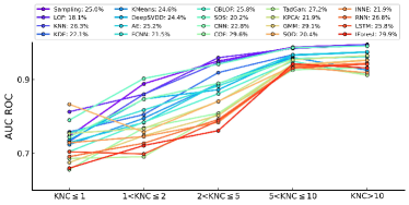
Figure 7: The performance of top 20 algorithms on AUC-ROC under different KNC.

5.5 The robustness of algorithms under KNC

In order to observe the robustness of various algorithms, we classify the difficulty of the data set according to KNC and observe the results of each algorithm under different difficulty data.

We first select 20 best-performing algorithms under AUC-ROC and observe their change in AUC-ROC values on the difficulty of the dataset, where all the algorithm achieve a AUC-ROC value of more than 0.9 on the dataset with KNC$>$10. Furthermore, we calculate the decline ratio of each algorithm (i.e. 1 - Min/Max performed at different difficulties). We find that the two most robust algorithms are LOF with 18.1$\%$ and SOS with 20.4$\%$, while the two worst ones are IForest with 29.9$\%$ and GMM with 29.1$\%$. The decline rate of most algorithms is concentrated between 20 and 30 percent. Furthermore, we also analyze the performance and change of each algorithm under different KNC, which is elaborated in Appendix C.4.

6 Acknowledgments

This work is sponsored by the National Key R$\&$D Program of China Grant No. 2022YFA1008200 (Z. X.), the Shanghai Sailing Program, the Natural Science Foundation of Shanghai Grant No. 20ZR1429000 (Z. X.), the National Natural Science Foundation of China Grant No. 62002221 (Z. X.), Shanghai Municipal of Science and Technology Major Project No. 2021SHZDZX0102, and the HPC of School of Mathematical Sciences and the Student Innovation Center, and the Siyuan-1 cluster supported by the Center for High Performance Computing at Shanghai Jiao Tong University.

Appendix A Appendix for Time Series Anomaly State Detection

A.1 Concrete operations of training stage and testing stage for implementation framework

Algorithm 2 Standard training procedure for time series anomaly state detection

1:  Input: standard time series data $X_{standard}\in\mathbb{R}^{n_{0}\times d_{0}}$, where $n_{0}$ is the length and $d_{0}$ is the dimension of features, feature extraction function $f:X\to Y$, time series anomaly state detection algorithm functions $\mathcal{H}:Y\to A$, de-windowing function $\omega:A\to H$, and decision function $\mathcal{D}$.

2:  Data Partition: Partition standard time series data $X_{standard}$ into training time series data $X_{train}\in\mathbb{R}^{n_{1}\times d_{0}}$ and validation time series data $X_{validation}\in\mathbb{R}^{n_{2}\times d_{0}}$, where $n_{0}=n_{1}+n_{2}$.

3:  Feature Extraction: Learn and extract features of training time series $X_{train}$ through feature extraction functions $f$ to obtain the training feature window data $Y_{train}=f_{train}(X_{train})\in\mathbb{R}^{n_{3}\times d_{1}}$, where $n_{3}$ is the number of feature windows and $d_{1}$ is the dimension of features after pre-processing. And then, Use $f_{train}$ to extract the features of validation time series data $X_{validation}$ and obtain the validation feature window data $Y_{validation}=f_{train}(X_{validation})\in\mathbb{R}^{n_{4}\times d_{1}}$, where $n_{4}$ is the number of feature windows.

4:  Model Training: Use the training feature window data $Y_{train}$ to train time series anomaly state detection algorithm functions $\mathcal{H}$, and get the trained algorithm $\mathcal{H}_{train}$.

5:  Model Inference: Calculate the anomaly score $A_{validation}=\mathcal{H}_{train}(Y_{validation})\in\mathbb{R}^{n_{4}\times 1}$ of the validation feature window data $Y_{validation}$ under the trained algorithm function $\mathcal{H}_{train}$.

6:  De-windowing: The de-windowing function $\omega$ is utilized to map the validation anomaly score $A_{validation}$ back to the length of the validation time series $X_{validation}$ to align with the original sequence, and get the modified validation anomaly score $\hat{A}_{validation}=\omega(A_{validation})\in\mathbb{R}^{n_{2}\times 1}$.

7:  Learning Decision Function: Use the modified validation anomaly score $\hat{A}_{validation}$ to learn the decision function $\mathcal{D}$, and get the learned decision function $\mathcal{D}_{validation}$.

Algorithm 3 Standard testing procedure for time series anomaly state detection

1:  Input: test time series data $X_{test}\in\mathbb{R}^{n_{5}\times d_{0}}$, where $n_{5}$ is the length and $d_{0}$ is the dimension of features, trained feature extraction function $f_{train}$, trained time series anomaly state detection algorithm function $\mathcal{H}_{train}$, de-windowing function $\omega$, trained decision function $\mathcal{H}_{validation}$, and decision threshold $T$.

2:  Feature Extraction: Use the trained feature extraction function $f_{train}$ to process the test time series $X_{test}$ to obtain the testing feature window data $Y_{test}=f_{train}(X_{test})\in\mathbb{R}^{n_{6}\times d_{1}}$.

3:  Model Inference: Use the trained algorithm function $\mathcal{H}_{train}$ to calculate the test anomaly score $A_{test}=\mathcal{H}_{train}(Y_{test})\in\mathbb{R}^{n_{6}\times 1}$ of the testing feature window data $Y_{test}$.

4:  De-windowing: The de-windowing function $\omega$ is utilized to map the test anomaly score $A_{test}$ back to the length of the test time series $X_{test}$ to align with the original sequence, and get the modified test anomaly score $\hat{A}_{test}=\omega(A_{test})\in\mathbb{R}^{n_{5}\times 1}$.

5:  Inferring Health Indicator Series: Use the trained decision function $\mathcal{D}_{train}$ to calculate the test health indicator series $H_{test}=\mathcal{D}_{train}(\hat{A}_{test})$ of the test time series $X_{test}$

6:  Determining Anomaly: Use decision threshold $T$ to determine whether an anomaly occurs in $X_{test}$, and finally get the healthy index $\hat{H}_{test}$. For a given point $h_{i}\in H_{test}$ in the test health indicator series $H_{test}$: if $h_{i}<T$, then the corresponding original test time series point $x_{i}\in X_{test}$ is considered as the inlier, and has $\hat{h}_{i}=0$; else if $h_{i}\geq T$, then the corresponding original test time series point $x_{i}\in X_{test}$ is considered as the outlier, and has $\hat{h}_{i}=1$.

A.2 Intuitive analysis for outliers under the implementation framework

A question of concern is, what do the anomalies we find look like in the implementation framework? When we find a point $h_{0}=d_{train}(\hat{a}_{0})\geq T,h_{0}\in H_{test},\hat{a}_{0}\in A_{test}$, then it means that $\hat{a}_{0}$ is relative large among $\hat{A}_{validation}$. Therefore, $A_{0}=w^{-1}(\hat{a}_{0})=h^{*}(Y_{0})$ is also relative large among $A_{validation}$, which infers that under trained algorithm function $h^{*}$, $Y_{0}$ is far away from all the feature windows in $Y_{validation}$.

In other words, if the ”distance” $d_{test}$ between a test feature window $Y_{0}\in Y_{test}$ and its closest training windows $Y_{train,0}$ compared to the average ”distance” $\bar{d}_{validation}$ between the validation windows $Y_{validation}$ and the training windows $Y_{train}$ is far, then it will result in $a_{0}=h^{*}(Y_{0})$ to be too large, and ultimately lead to $h_{0}=d_{train}(\hat{a}_{0})$ being too large. Then we consider the test feature window $Y_{0}$ to be abnormal, and its corresponding original time series segment $X_{0}$ to be abnormal.

Therefore, if a pattern segment in the test time series has never appeared in the standard time series, then it will easily lead to the test feature window $Y_{0}\in Y_{test}$ containing this pattern far away from the validation feature windows $Y_{validation}$ and makes the corresponding health indicator exceed the decision threshold $T$. Therefore, we define anomalies in the time series anomaly state detection problem as follows.

Intuitive Definition for Outliers under specific implementation: If a pattern in test time series does not appear in standard time series, then we call this pattern an anomaly.

Formal Definition for Outliers under specific implementation: Given a suitable threshold $\epsilon$, a distance function $d(X,Y)$ and a sequence length $n_{0}$, if there exists a dimension $d_{0}$ of a test time series data segment $\hat{X}_{0,d_{0}}^{test}\in\mathbb{R}^{n_{0}}$, such that $\hat{X}_{0,d_{0}}^{test}$ is inconsistent with any segment of this dimension $d_{0}$ in the standard time series data segments $\{\hat{X}_{i,d_{0}}^{standard}\in\mathbb{R}^{n_{0}}\}_{i\in\mathbb{N}}$ with the same length $n_{0}$, that is, $d(\hat{X}_{0,d_{0}}^{test},\hat{X}_{i,d_{0}}^{standard})>\epsilon$ for all $i\in\mathbb{N}$ , then it is said that under the threshold $\epsilon$, the distance function $d(X,Y)$ and the sequence length $n_{0}$, the test data segment$\hat{X}_{0}^{test}$ is abnormal from the standard time series data.

Note that the sequence length $n_{0}$ here is similar to the process of windowing, which is a very important parameter in the time series. Such a definition is also consistent with the mathematical definition in Sec. 3.1. Specifically, in mathematical definition, we believe that outliers are those segments that do not follow the standard random process, $\mathcal{O}=\{S_{j}^{k}\subset\{\hat{x}_{j}(t),t\in[\hat{N}_{j}]\}\in\mathcal{U}:S_{j}^{k}\nsim\{X_{0}(t),t\in\mathbb{N}\}\}$, so in specific practice, we identify those test time series segments that are far away from the standard time series as ones not obeying the standard random process, which is very reasonable and consistent.

Appendix B Appendix for preparation for experiments

B.1 The time series anomaly state detection algorithms list

Forecast-based methods refer to time series anomaly detection approaches , wherein predictive models are trained to anticipate future values first, and subsequently, identify the anomaly by assessing the disparity between the predicted values and the actual observed values. This method constitutes the prevailing and prevalent technique within the realm of time series anomaly detection. LinearRegreesion(LR) utilizes a high-dimensional linear model to act as a prediction function and assumes that each moment is linearly related to several previous moments. Fully connected neural networks (FCNN), Convolutional neural networks (CNN), Recurrent Neural Network (RNN), Gated Recurrent Unit (GRU), and Long Short-Term Memory (LSTM) respectively use corresponding neural networks structure to serve as prediction models and analyse the nonlinear temporal correlations between data samples. It is worth mentioning that the model design of RNN, GRU and LSTM makes them further take into account the time correlation of the data itself, which is more in line with the characteristics of time series data.

Reconstitution-based methods aim to learn a model that captures the latent structure of the given time series data and generate synthetic reconstructions, and then discriminate the anomaly by reconstruction performance under assumption that outliers cannot be efficiently reconstructed from the low-dimensional mapping space. Auto-Encoder (VAE) and Variational Auto-Encoder (VAE) use the Encoder neural network to map the time series data to low-dimensional latent space and normal distribution respectively, and then use the Decoder neural network to reconstruct the original data. Kernel Principal Component Analysis (KPCA) maps data to the feature space generated by the kernel and uses the reconstruction error on the feature space to determine anomalies. Transformer uses the Transformer structure to compress and reconstruct data, whose main feature is that it has a special attention structure to consider the temporal correlation of data. Time Series Anomaly Detection with Generative Adversarial Networks (TanoGan) and Time Series Anomaly Detection Using Generative Adversarial Networks (TadGan) are both algorithms based on adversarial generative neural networks, and use LSTM as the generator and discriminator model to gradually learn the real data distribution through adversarial generation. However, during the reconstruction process, TanoGan uses the residual loss and discriminant loss between the real sequence and its closest generated sequence to identify anomalies; while TadGan uses the cyele consistency loss of the time series and the value of its discriminator to distinguish anomalies.

Statistical-model-based methods assume that the data is generated by a certain statistical distribution, and use statistical models to perform hypothesis testing to determine which data does not meet the model assumptions, thereby detecting outliers. Copula-Based Outlier Detection (COPOD) is a non-parametric method, which obtain the empirical copula through the empirical cumulative distribution , and then estimate the tail probability of the joint distribution in all dimensions. The Empirical Cumulative Distribution-Based Outlier Detection (ECOD) method undertakes the computation of the empirical cumulative distribution for each dimension within the training dataset, and Subsequently, amalgamates the tail probabilities associated with each dimension as a means of deriving the anomaly score. Through the representation of data as a composite of Gaussian components, Gaussian Mixture Models (GMMs) have the capacity to distinguish anomalies by detecting data points that exhibit substantial deviations from the acquired distribution. Histogram- based outlier detection (HBOS) assumes feature independence and utilizes histograms to measure data point outlierness, where the inverse of the bin height serves as the outlier score. Kernel density estimation (KDE) is a non-parametric method that applies kernel smoothing to probability density estimation, that is, using the kernel as a weight to estimate the probability density function of random variables, and then calculates the density estimate of the data points and compares it with the threshold Compare to identify outliers. Lightweight on-line detector of anomalies (LODA) utilizes one-dimensional histograms constructed on sparse random projections, where anomaly score is a negative average log probability estimated from histogram on projections. Random sparse projects allow LODA to use simple one-dimensional histograms, thus processing large datasets in relatively small time complexity. Mean Absolute Differences (MAD) Algorithm determines whether an anomaly has occurred by calculating the median of the absolute deviation from the data point to the median. Outlier Detection with Minimum Covariance Determinant (MCD) is a powerful method for detecting outliers in multivariate data by estimating a robust covariance matrix and using Mahalanobis distances to quantify the outlier degree of each data point.

Proximity-based methods for anomaly detection are techniques that primarily rely on using various distance measures to quantify the similarity or proximity between data points, including density, distance, angle and dividing hyperplane, and then identify anomalies, under the assumption that the distribution of abnormal points is different from that of normal points, causing the similarity is low. Angle-based outlier detection (ABOD) considers the variance of an observation’s weighted cosine score relative to all its neighbors as its outlying score. Cluster-Based Local Outlier Factor (CBLOF) first use a clustering algorithm to divide the data into large clusters and small clusters, and then calculate the distance from each point to the nearest large cluster as anomaly score. Cook’s distance outlier detection (CD) measure the influence of observations on a linear regression, and identify instances with large influence as outliers. Connectivity-Based Outlier Factor (COF) calculates the ratio of the average chaining distance of an oberservation to the average chaining distance of its k-th nearest neighbor as the anomaly score. Deep One-Class Classification for outlier detection (DeepSVDD) minimize the volume of hyper-sphere that enfolds the sample feature space represented by a neural network, and then calculate the distance between the center of the sphere and the sample as anomaly score. Isolation forest (IForest) constructs a random forest of binary trees to isolate the data points and identifies data points with shorter average path lengths to the root as anomalies. Isolation-based anomaly detection using nearest-neighbor ensembles (INNE) uses a multi-dimensional hypersphere to cut the data space to implement the isolation mechanism, and takes into account the local distribution characteristics of the data, the nearest neighbor distance ratio, to calculate anomaly indicators of the data. The Kmeans outlier detector (Kmeans) first finds K clusters through iteration, and then calculates the distance between the observation and the center of its nearest cluster as an outlier score. K-Nearest Neighbors (KNN) consider the anomaly score of the observation as the distance to its nearest k neighbors. Local Outlier Factor (LOF) measures the local deviation in the density of a particular data point relative to that of its neighboring points, where the local density around a given data point is estimated by the distances to its k nearest neighboring data points. One-class SVM (OCSVM) aims to find a separating hyperplane that best separates the origin from the majority of normal data points, which is also defined as the decision boundary. The PCA algorithm (PCA) maps the data onto a low-dimensional hyperplane generated by the principal components of the data, and treats points far away from this hyperplane as anomalies. Quasi-Monte Carlo Discrepancy outlier detection (QMCD) uses Wrap-around Quasi-Monte Carlo Discrepancy, a uniformity criterion which is used to assess the space filling of a number of samples in a hypercube, to calculate the discrepancy values of the sample as anomaly scores. Outlier detection based on Sampling (SP) first randomly and independently sample a subset of the data, and then view the distance between the observation and the subset as anomaly score. Subspace Outlier Detection (SOD) explores a axis-parallel subspace spanned by the data object’s neighbors and calculates the degree how much it deviates from the neighbors in this subspace as the anomaly score. Stochastic outlier selection (SOS) employs the concept of affinity to quantify the relationship of one data point to another, where a data point is considered to be an outlier when the other data points have insufficient affinity with it. One-Classification using Support Vector Data Description (SVDD) establish a hyper-sphere with the smallest radius in a high-dimensional space, and then calculating the distance between the sample point and the hyper-sphere as anomaly score.

B.2 Details for relative contrast, normalized clusteredness, and normalized adjacency

Previous articles have discussed several indicators to measure the difference in distribution of normal points and abnormal points, including Relative Contrast (RC) (He et al., 2012), which is defined as the ratio of the expectation of the mean distance to the expectation of nearest neighbor distance for all data points, Normalized clusteredness of abnormal points (NC) (Emmott et al., 2013), which is the ratio of the average SBD of normal subsequences to the average SBD of abnormal subsequences, and Normalized adjacency of normal/abnormal cluster (NA) (Paparrizos et al., 2022b), which is defined as the ratio of the minimum distance between the centroids of normal and abnormal clusters to the average distance among the centroids of all normal clusters.

$$R_{c}=\frac{\mathbb{E}_{s\in S}\left[D_{\text{mean}}(s)\right]}{\mathbb{E}_{s\in S}\left[D_{\min}(s)\right]},\ N_{c}=\frac{\mathbb{E}_{s_{i},s_{j}\in S_{\text{nor},i\neq j}}\left[D\left(s_{i},s_{j}\right)\right]}{\mathbb{E}_{s_{i},s_{j}\in S_{\text{ano },i\neq j}}\left[D\left(s_{i},s_{j}\right)\right]},\ N_{a}=\frac{\min_{c_{i}\in C_{ano},c_{j}\in C_{nor}}D\left(c_{i},c_{j}\right)}{\mathbb{E}_{c_{i},c_{j}\in C_{nor},i\neq j}\left[D\left(c_{i},c_{j}\right)\right]}$$ (4)

where $s$ represents time series, $D(s_{i},s_{j})$ is denoted as the SBD distance between two series $s_{i}$ and $s_{j}$, $S$ is the whole set, $D_{\min}(x)=\min_{s\in S-x}D(x,s)$ and $D_{\text{mean }}(x)=\mathbb{E}_{s\in S-x}D(x,s)$ are the 1-NN distance and mean distance fot series $x$, $S_{nor}$ and $S_{ano}$ are denoted as the set of normal sequences and the set of anomalous sequence, and $C_{nor}$ and $C_{ano}$ are denoted as the set of centroids of normal clusters and the set of centroids of anomalous clusters.

Appendix C Appendix for experiments

C.1 More results for performance of algorithms under eight representative accuracy evaluation measures

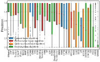
(a) Precision

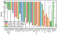
(b) Recall

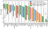
(c) F1-score

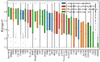
(d) Range-F1

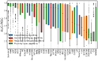
(e) AUC-ROC

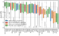
(f) AUC-PR

(g) VUS-ROC

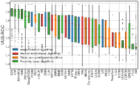
(h) VUS-PR

Figure 8: Performance of algorithms under eight representative accuracy evaluation measures. The sub-caption of (a-h) indicate the evaluation measures used.

C.2 More results for critical differnece of algorithms under eight representative accuracy evaluation measures

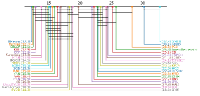
(a) Precision

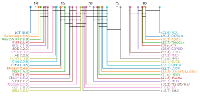
(b) Recall

(c) F1-score

(d) Range-f1

(e) AUC-ROC

(f) AUC-PR

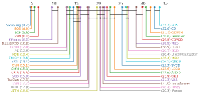
(g) VUS-ROC

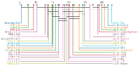
(h) VUS-PR

Figure 9: Critical Difference of algorithms under eight representative accuracy evaluation measures. The sub-caption of (a-h) indicate the evaluation measures used.

C.3 More results for performance of four types of algorithms under eight representative accuracy evaluation measures

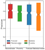
(a) Precision

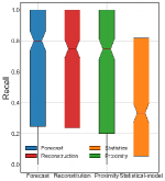
(b) Recall

(c) F1-score

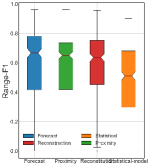
(d) Range-f1

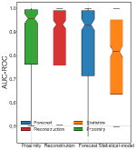
(e) AUC-ROC

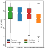
(f) AUC-PR

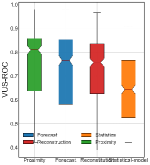
(g) VUS-ROC

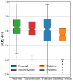
(h) VUS-PR

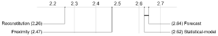
(i) Critical Difference under Precision

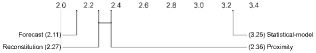
(j) Critical Difference under Recall

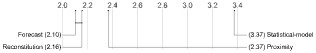
(k) Critical Difference under F1-score

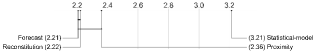
(l) Critical Difference under Range-f1

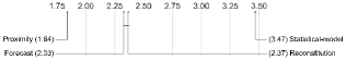
(m) Critical Difference under AUC-ROC

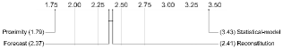
(n) Critical Difference under AUC-PR

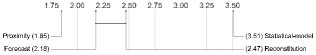
(o) Critical Difference under VUS-ROC

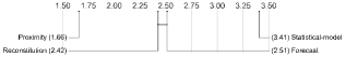
(p) Critical Difference under VUS-PR

Figure 10: Performance and Critical Difference of four types of algorithms under eight representative accuracy evaluation measures. The sub-caption of (a-p) indicate the evaluation measures used.

C.4 More results for algorthms performance under KNC

Table 2: Average value of eight representative accuracy evaluation measures for all the thirty-eight algorithms.

Metrics 1	Precision	Recall	F1	Range-F1	AUC-ROC	AUC-PR	VUS-ROC	VUS-PR
ABOD	0.183	0.200	0.158	0.174	0.797	0.775	0.664	0.650
AE	0.743	0.729	0.613	0.655	0.907	0.802	0.785	0.680
CBLOF	0.799	0.631	0.562	0.656	0.879	0.773	0.771	0.664
CD	0.378	0.197	0.165	0.253	0.596	0.583	0.514	0.510
CNN	0.739	0.690	0.567	0.633	0.876	0.741	0.757	0.629
COF	0.815	0.591	0.543	0.650	0.858	0.724	0.765	0.624
COPOD	0.412	0.220	0.207	0.297	0.678	0.425	0.572	0.359
DeepSVDD	0.754	0.807	0.644	0.680	0.913	0.764	0.816	0.677
ECOD	0.452	0.247	0.232	0.341	0.686	0.428	0.580	0.370
FCNN	0.813	0.696	0.596	0.663	0.881	0.753	0.776	0.653
GMM	0.683	0.672	0.553	0.614	0.861	0.684	0.751	0.588
GRU	0.581	0.579	0.463	0.508	0.822	0.628	0.696	0.524
HBOS	0.721	0.488	0.448	0.549	0.810	0.686	0.692	0.583
IForest	0.730	0.520	0.474	0.568	0.838	0.707	0.710	0.595
INNE	0.708	0.581	0.505	0.577	0.844	0.740	0.732	0.646
KDE	0.812	0.776	0.641	0.690	0.921	0.811	0.792	0.688
KMeans	0.818	0.689	0.614	0.685	0.895	0.803	0.795	0.700
KNN	0.798	0.799	0.686	0.719	0.949	0.857	0.847	0.749
KPCA	0.602	0.724	0.560	0.574	0.883	0.705	0.765	0.606
LinearRegression	0.450	0.459	0.352	0.403	0.746	0.501	0.645	0.422
LODA	0.693	0.466	0.395	0.510	0.785	0.640	0.664	0.565
LOF	0.750	0.873	0.713	0.701	0.953	0.851	0.865	0.762
LSTM	0.578	0.621	0.485	0.527	0.827	0.649	0.713	0.547
MAD	0.582	0.357	0.320	0.406	0.752	0.581	0.616	0.502
MCD	0.511	0.472	0.366	0.435	0.751	0.537	0.631	0.441
MSD	0.493	0.290	0.259	0.341	0.704	0.510	0.583	0.450
OCSVM	0.466	0.153	0.161	0.311	0.614	0.387	0.533	0.355
PCA	0.275	0.066	0.085	0.177	0.566	0.332	0.499	0.314
QMCD	0.053	0.443	0.074	0.074	0.654	0.663	0.598	0.595
RNN	0.600	0.636	0.507	0.554	0.841	0.667	0.729	0.571
Sampling	0.841	0.818	0.718	0.762	0.956	0.873	0.858	0.769
SOD	0.771	0.678	0.567	0.630	0.875	0.714	0.752	0.607
SOS	0.510	0.825	0.535	0.476	0.955	0.851	0.883	0.740
SVDD	0.642	0.421	0.362	0.491	0.757	0.567	0.640	0.513
TadGan	0.804	0.582	0.523	0.622	0.843	0.736	0.733	0.639
TanoGan	0.446	0.176	0.193	0.313	0.651	0.529	0.541	0.481
Transformer	0.675	0.510	0.441	0.519	0.806	0.620	0.685	0.531
VAE	0.691	0.559	0.481	0.541	0.831	0.692	0.698	0.576

Table 3: Average value of eight representative accuracy evaluation measures for all the thirty-eight algorithms when KNC$>$10

Metrics 1	Precision	Recall	F1	Range-F1	AUC-ROC	AUC-PR	VUS-ROC	VUS-PR
ABOD	0.108	0.131	0.111	0.113	0.806	0.816	0.686	0.676
AE	0.753	0.952	0.772	0.738	0.975	0.914	0.878	0.806
CBLOF	0.841	0.801	0.708	0.755	0.913	0.854	0.840	0.755
CD	0.555	0.360	0.350	0.447	0.715	0.668	0.591	0.559
CNN	0.835	0.921	0.763	0.774	0.964	0.887	0.878	0.789
COF	0.886	0.765	0.704	0.771	0.932	0.851	0.853	0.747
COPOD	0.570	0.362	0.345	0.451	0.779	0.513	0.654	0.436
DeepSVDD	0.758	0.961	0.752	0.722	0.974	0.857	0.897	0.782
ECOD	0.584	0.377	0.359	0.480	0.765	0.489	0.645	0.426
FCNN	0.899	0.893	0.752	0.782	0.961	0.882	0.880	0.793
GMM	0.748	0.867	0.709	0.730	0.953	0.804	0.856	0.709
GRU	0.706	0.846	0.674	0.670	0.931	0.779	0.821	0.675
HBOS	0.860	0.645	0.609	0.716	0.890	0.807	0.776	0.688
IForest	0.869	0.750	0.699	0.759	0.931	0.872	0.818	0.727
INNE	0.818	0.821	0.705	0.725	0.918	0.871	0.835	0.768
KDE	0.923	0.960	0.796	0.817	0.973	0.919	0.870	0.805
KMeans	0.815	0.822	0.730	0.737	0.925	0.883	0.857	0.799
KNN	0.782	0.991	0.824	0.768	0.993	0.944	0.927	0.860
KPCA	0.661	0.950	0.702	0.642	0.965	0.836	0.874	0.752
LinearRegression	0.528	0.698	0.499	0.500	0.861	0.626	0.751	0.538
LODA	0.821	0.753	0.651	0.703	0.907	0.830	0.792	0.712
LOF	0.728	0.998	0.792	0.701	0.991	0.924	0.931	0.850
LSTM	0.695	0.879	0.692	0.683	0.941	0.815	0.844	0.718
MAD	0.768	0.534	0.481	0.570	0.836	0.661	0.699	0.581
MCD	0.612	0.667	0.495	0.557	0.839	0.665	0.717	0.557
MSD	0.637	0.437	0.386	0.460	0.777	0.561	0.649	0.512
OCSVM	0.667	0.292	0.295	0.487	0.684	0.442	0.580	0.406
PCA	0.451	0.120	0.159	0.292	0.602	0.318	0.521	0.316
QMCD	0.081	0.643	0.110	0.105	0.752	0.754	0.673	0.648
RNN	0.731	0.893	0.716	0.718	0.944	0.831	0.853	0.739
Sampling	0.807	0.991	0.839	0.793	0.995	0.948	0.931	0.867
SOD	0.844	0.815	0.724	0.762	0.952	0.845	0.851	0.740
SOS	0.557	0.888	0.624	0.493	0.990	0.963	0.933	0.848
SVDD	0.743	0.678	0.565	0.648	0.857	0.715	0.734	0.625
TadGan	0.829	0.764	0.662	0.717	0.912	0.845	0.817	0.743
TanoGan	0.687	0.387	0.384	0.527	0.752	0.627	0.618	0.563
Transformer	0.749	0.745	0.621	0.657	0.898	0.743	0.793	0.655
VAE	0.851	0.803	0.697	0.708	0.923	0.853	0.814	0.727

Table 4: Average value of eight representative accuracy evaluation measures for all the thirty-eight algorithms when 5$<$KNC$<$10

Metrics 1	Precision	Recall	F1	Range-F1	AUC-ROC	AUC-PR	VUS-ROC	VUS-PR
ABOD	0.261	0.324	0.254	0.273	0.885	0.862	0.718	0.685
AE	0.788	0.920	0.748	0.759	0.966	0.905	0.841	0.748
CBLOF	0.856	0.779	0.683	0.750	0.949	0.868	0.828	0.726
CD	0.460	0.179	0.163	0.268	0.614	0.591	0.491	0.491
CNN	0.834	0.910	0.718	0.750	0.955	0.862	0.845	0.733
COF	0.828	0.756	0.672	0.743	0.926	0.793	0.831	0.667
COPOD	0.418	0.205	0.204	0.285	0.683	0.418	0.568	0.337
DeepSVDD	0.724	0.941	0.709	0.726	0.965	0.828	0.853	0.723
ECOD	0.433	0.226	0.212	0.326	0.691	0.400	0.570	0.329
FCNN	0.878	0.905	0.738	0.764	0.956	0.845	0.851	0.740
GMM	0.720	0.864	0.674	0.706	0.939	0.807	0.823	0.678
GRU	0.671	0.772	0.585	0.617	0.912	0.729	0.751	0.577
HBOS	0.866	0.640	0.588	0.673	0.898	0.760	0.759	0.636
IForest	0.856	0.709	0.650	0.728	0.942	0.834	0.793	0.684
INNE	0.856	0.743	0.652	0.723	0.933	0.817	0.798	0.691
KDE	0.875	0.945	0.757	0.783	0.967	0.895	0.841	0.752
KMeans	0.887	0.887	0.773	0.804	0.959	0.900	0.861	0.766
KNN	0.805	0.959	0.807	0.786	0.985	0.934	0.896	0.821
KPCA	0.640	0.919	0.683	0.652	0.953	0.828	0.835	0.708
LinearRegression	0.481	0.681	0.480	0.490	0.838	0.585	0.707	0.477
LODA	0.775	0.616	0.518	0.612	0.860	0.715	0.708	0.608
LOF	0.717	0.982	0.763	0.704	0.984	0.912	0.907	0.829
LSTM	0.693	0.862	0.636	0.661	0.931	0.788	0.792	0.647
MAD	0.645	0.420	0.384	0.472	0.797	0.578	0.630	0.490
MCD	0.610	0.651	0.474	0.500	0.846	0.628	0.679	0.490
MSD	0.547	0.318	0.299	0.404	0.725	0.499	0.583	0.426
OCSVM	0.500	0.163	0.169	0.323	0.637	0.395	0.535	0.352
PCA	0.276	0.056	0.075	0.174	0.574	0.347	0.498	0.315
QMCD	0.051	0.537	0.070	0.068	0.696	0.695	0.615	0.598
RNN	0.731	0.860	0.655	0.675	0.934	0.800	0.801	0.669
Sampling	0.843	0.962	0.833	0.826	0.987	0.947	0.902	0.842
SOD	0.816	0.806	0.653	0.703	0.936	0.800	0.794	0.661
SOS	0.533	0.918	0.593	0.516	0.986	0.934	0.913	0.802
SVDD	0.711	0.543	0.445	0.554	0.813	0.597	0.661	0.531
TadGan	0.881	0.839	0.711	0.760	0.942	0.860	0.807	0.716
TanoGan	0.635	0.317	0.332	0.453	0.745	0.625	0.597	0.538
Transformer	0.694	0.553	0.483	0.536	0.838	0.634	0.694	0.520
VAE	0.804	0.740	0.597	0.633	0.924	0.770	0.729	0.595

Table 5: Average value of eight representative accuracy evaluation measures for all the thirty-eight algorithms when 2$<$KNC$<$5

Metrics 1	Precision	Recall	F1	Range-F1	AUC-ROC	AUC-PR	VUS-ROC	VUS-PR
ABOD	0.189	0.190	0.156	0.175	0.784	0.759	0.663	0.656
AE	0.779	0.605	0.546	0.643	0.888	0.745	0.759	0.630
CBLOF	0.807	0.502	0.479	0.620	0.861	0.740	0.747	0.639
CD	0.277	0.082	0.075	0.163	0.538	0.535	0.488	0.487
CNN	0.842	0.684	0.610	0.692	0.889	0.738	0.764	0.628
COF	0.779	0.469	0.453	0.582	0.808	0.657	0.715	0.568
COPOD	0.407	0.182	0.172	0.281	0.648	0.426	0.554	0.372
DeepSVDD	0.799	0.699	0.592	0.662	0.872	0.714	0.772	0.631
ECOD	0.451	0.216	0.205	0.311	0.661	0.442	0.567	0.392
FCNN	0.864	0.681	0.614	0.695	0.882	0.730	0.772	0.638
GMM	0.673	0.527	0.457	0.556	0.802	0.602	0.694	0.518
GRU	0.653	0.467	0.414	0.511	0.783	0.587	0.659	0.490
HBOS	0.665	0.336	0.318	0.446	0.736	0.603	0.629	0.523
IForest	0.624	0.351	0.311	0.425	0.761	0.602	0.643	0.521
INNE	0.619	0.399	0.368	0.469	0.784	0.660	0.673	0.594
KDE	0.836	0.695	0.604	0.679	0.918	0.773	0.783	0.661
KMeans	0.861	0.574	0.546	0.675	0.888	0.770	0.778	0.667
KNN	0.848	0.722	0.650	0.730	0.945	0.843	0.827	0.722
KPCA	0.617	0.579	0.486	0.559	0.840	0.624	0.716	0.527
LinearRegression	0.402	0.258	0.232	0.326	0.653	0.413	0.571	0.356
LODA	0.616	0.261	0.227	0.377	0.703	0.519	0.597	0.486
LOF	0.811	0.843	0.722	0.751	0.959	0.843	0.859	0.748
LSTM	0.638	0.498	0.431	0.516	0.788	0.593	0.661	0.491
MAD	0.509	0.233	0.225	0.324	0.701	0.560	0.579	0.491
MCD	0.403	0.297	0.252	0.340	0.666	0.446	0.569	0.375
MSD	0.447	0.199	0.189	0.281	0.667	0.503	0.560	0.449
OCSVM	0.366	0.080	0.094	0.230	0.577	0.363	0.515	0.351
PCA	0.188	0.035	0.047	0.119	0.546	0.344	0.495	0.335
QMCD	0.043	0.280	0.056	0.060	0.619	0.626	0.579	0.584
RNN	0.652	0.499	0.432	0.530	0.791	0.600	0.670	0.503
Sampling	0.883	0.739	0.680	0.766	0.950	0.855	0.836	0.737
SOD	0.781	0.641	0.523	0.598	0.841	0.655	0.722	0.546
SOS	0.536	0.771	0.516	0.488	0.941	0.801	0.869	0.707
SVDD	0.611	0.267	0.251	0.426	0.704	0.513	0.606	0.479
TadGan	0.835	0.481	0.453	0.593	0.808	0.674	0.697	0.594
TanoGan	0.717	0.258	0.289	0.454	0.707	0.620	0.584	0.553
Transformer	0.670	0.391	0.350	0.478	0.761	0.573	0.642	0.502
VAE	0.619	0.375	0.348	0.451	0.763	0.596	0.648	0.510

Table 6: Average value of eight representative accuracy evaluation measures for all the thirty-eight algorithms when 1$<$KNC$<$2

Metrics 1	Precision	Recall	F1	Range-F1	AUC-ROC	AUC-PR	VUS-ROC	VUS-PR
ABOD	0.190	0.168	0.115	0.140	0.709	0.640	0.578	0.561
AE	0.612	0.419	0.353	0.440	0.783	0.626	0.639	0.511
CBLOF	0.658	0.457	0.367	0.477	0.784	0.610	0.654	0.513
CD	0.213	0.201	0.073	0.129	0.515	0.538	0.480	0.502
CNN	0.804	0.551	0.492	0.614	0.846	0.696	0.708	0.568
COF	0.757	0.377	0.332	0.488	0.769	0.581	0.659	0.494
COPOD	0.205	0.113	0.086	0.129	0.587	0.305	0.497	0.249
DeepSVDD	0.711	0.639	0.514	0.606	0.847	0.652	0.742	0.560
ECOD	0.283	0.153	0.135	0.217	0.618	0.343	0.522	0.291
FCNN	0.826	0.478	0.443	0.574	0.817	0.652	0.689	0.533
GMM	0.578	0.429	0.365	0.452	0.748	0.522	0.622	0.443
GRU	0.510	0.283	0.265	0.368	0.701	0.532	0.574	0.440
HBOS	0.460	0.366	0.293	0.361	0.732	0.572	0.609	0.475
IForest	0.571	0.279	0.240	0.361	0.721	0.506	0.576	0.426
INNE	0.544	0.380	0.296	0.393	0.745	0.612	0.613	0.516
KDE	0.551	0.472	0.358	0.431	0.805	0.631	0.644	0.500
KMeans	0.664	0.477	0.386	0.494	0.795	0.639	0.664	0.545
KNN	0.728	0.496	0.425	0.560	0.860	0.676	0.720	0.562
KPCA	0.458	0.443	0.350	0.423	0.767	0.521	0.617	0.418
LinearRegression	0.397	0.219	0.207	0.301	0.642	0.387	0.552	0.310
LODA	0.564	0.258	0.200	0.362	0.672	0.502	0.550	0.449
LOF	0.709	0.638	0.539	0.615	0.860	0.697	0.741	0.591
LSTM	0.508	0.293	0.267	0.369	0.698	0.547	0.577	0.441
MAD	0.370	0.254	0.183	0.239	0.670	0.502	0.545	0.420
MCD	0.450	0.296	0.261	0.357	0.668	0.412	0.564	0.340
MSD	0.313	0.216	0.156	0.204	0.639	0.461	0.529	0.388
OCSVM	0.323	0.080	0.088	0.203	0.559	0.337	0.496	0.286
PCA	0.195	0.062	0.064	0.128	0.545	0.304	0.478	0.264
QMCD	0.038	0.358	0.066	0.068	0.533	0.560	0.510	0.532
RNN	0.539	0.305	0.279	0.399	0.727	0.543	0.601	0.424
Sampling	0.815	0.559	0.491	0.644	0.888	0.722	0.749	0.610
SOD	0.597	0.392	0.321	0.412	0.758	0.531	0.617	0.462
SOS	0.365	0.721	0.375	0.379	0.903	0.688	0.810	0.571
SVDD	0.470	0.189	0.175	0.312	0.645	0.421	0.545	0.393
TadGan	0.624	0.203	0.231	0.380	0.691	0.544	0.592	0.474
TanoGan	0.646	0.231	0.226	0.387	0.697	0.587	0.572	0.522
Transformer	0.546	0.350	0.300	0.378	0.722	0.511	0.602	0.420
VAE	0.454	0.328	0.278	0.360	0.716	0.547	0.589	0.458

Table 7: Average value of eight representative accuracy evaluation measures for all the thirty-eight algorithms when KNC$<$1

Metrics 1	Precision	Recall	F1	Range-F1	AUC-ROC	AUC-PR	VUS-ROC	VUS-PR
ABOD	0.000	0.000	0.000	0.000	0.500	0.694	0.493	0.688
AE	1.000	0.312	0.380	0.558	0.729	0.796	0.682	0.749
CBLOF	1.000	0.334	0.351	0.548	0.705	0.737	0.644	0.689
CD	0.344	0.020	0.038	0.180	0.516	0.694	0.493	0.678
CNN	1.000	0.383	0.482	0.679	0.744	0.817	0.673	0.754
COF	1.000	0.152	0.252	0.652	0.656	0.761	0.617	0.703
COPOD	0.224	0.009	0.017	0.171	0.520	0.610	0.483	0.576
DeepSVDD	1.000	0.413	0.502	0.581	0.736	0.799	0.666	0.747
ECOD	0.894	0.035	0.066	0.430	0.601	0.685	0.547	0.634
FCNN	1.000	0.479	0.513	0.696	0.755	0.814	0.673	0.744
GMM	0.462	0.500	0.376	0.431	0.675	0.517	0.665	0.498
GRU	0.700	0.325	0.353	0.493	0.677	0.591	0.632	0.544
HBOS	0.000	0.000	0.000	0.000	0.513	0.702	0.494	0.675
IForest	0.500	0.121	0.193	0.377	0.660	0.766	0.620	0.729
INNE	0.500	0.446	0.410	0.415	0.729	0.813	0.674	0.766
KDE	0.500	0.456	0.400	0.398	0.758	0.823	0.674	0.755
KMeans	1.000	0.462	0.459	0.595	0.723	0.737	0.675	0.706
KNN	1.000	0.169	0.261	0.592	0.732	0.758	0.688	0.722
KPCA	0.429	0.469	0.429	0.414	0.754	0.826	0.703	0.767
LinearRegression	0.440	0.325	0.340	0.422	0.630	0.473	0.618	0.460
LODA	0.500	0.033	0.062	0.216	0.668	0.789	0.617	0.745
LOF	1.000	0.579	0.518	0.708	0.812	0.842	0.742	0.787
LSTM	0.896	0.521	0.428	0.542	0.704	0.695	0.640	0.653
MAD	0.500	0.275	0.355	0.421	0.700	0.814	0.643	0.763
MCD	0.438	0.413	0.354	0.408	0.655	0.481	0.644	0.467
MSD	0.500	0.294	0.370	0.428	0.701	0.814	0.643	0.763
OCSVM	0.500	0.011	0.022	0.205	0.535	0.694	0.510	0.653
PCA	0.000	0.000	0.000	0.000	0.524	0.694	0.497	0.678
QMCD	0.000	0.000	0.000	0.000	0.539	0.694	0.527	0.678
RNN	0.945	0.511	0.408	0.597	0.691	0.611	0.651	0.594
Sampling	1.000	0.316	0.406	0.671	0.746	0.776	0.695	0.730
SOD	1.000	0.989	0.695	0.798	0.833	0.772	0.770	0.731
SOS	0.813	1.000	0.655	0.698	0.790	0.761	0.740	0.711
SVDD	1.000	0.299	0.393	0.575	0.698	0.799	0.646	0.747
TadGan	1.000	0.332	0.367	0.552	0.686	0.704	0.633	0.678
TanoGan	0.560	0.036	0.066	0.338	0.544	0.718	0.524	0.688
Transformer	1.000	0.231	0.340	0.505	0.689	0.801	0.613	0.738
VAE	1.000	0.477	0.383	0.538	0.686	0.764	0.616	0.723

Table 8: Average value of eight representative accuracy evaluation measures for four types of algorithms.

Metrics 1	Precision	Recall	F1	Range-F1	AUC-ROC	AUC-PR	VUS-ROC	VUS-PR
Forecast-based	0.591	0.628	0.496	0.540	0.834	0.658	0.721	0.559
-based	0.683	0.571	0.502	0.558	0.837	0.699	0.715	0.591
Statistical-model-based	0.582	0.466	0.366	0.435	0.752	0.581	0.631	0.502
Proximity-based	0.730	0.591	0.535	0.577	0.858	0.740	0.752	0.646

Table 9: Average value of eight representative accuracy evaluation measures for four types of algorithms when KNC$>$10

Metrics 1	Precision	Recall	F1	Range-F1	AUC-ROC	AUC-PR	VUS-ROC	VUS-PR
Forecast-based	0.719	0.886	0.704	0.701	0.943	0.823	0.849	0.729
-based	0.751	0.783	0.680	0.682	0.917	0.840	0.815	0.735
Statistical-model-based	0.748	0.645	0.495	0.570	0.839	0.665	0.717	0.581
Proximity-based	0.758	0.801	0.704	0.722	0.925	0.854	0.840	0.747

Table 10: Average value of eight representative accuracy evaluation measures for four types of algorithms when 5$<$KNC$<$10.

Metrics 1	Precision	Recall	F1	Range-F1	AUC-ROC	AUC-PR	VUS-ROC	VUS-PR
Forecast-based	0.712	0.861	0.645	0.668	0.932	0.794	0.796	0.658
-based	0.741	0.789	0.640	0.643	0.933	0.799	0.768	0.651
Statistical-model-based	0.645	0.616	0.474	0.500	0.846	0.628	0.679	0.490
Proximity-based	0.724	0.756	0.652	0.704	0.936	0.828	0.798	0.685

Table 11: Average value of eight representative accuracy evaluation measures for four types of algorithms when 2$<$KNC$<$5

Metrics 1	Precision	Recall	F1	Range-F1	AUC-ROC	AUC-PR	VUS-ROC	VUS-PR
Forecast-based	0.653	0.499	0.432	0.523	0.790	0.597	0.665	0.497
-based	0.693	0.436	0.401	0.518	0.785	0.622	0.673	0.540
Statistical-model-based	0.509	0.261	0.227	0.340	0.701	0.519	0.579	0.486
Proximity-based	0.624	0.469	0.453	0.488	0.808	0.660	0.715	0.594

Table 12: Average value of eight representative accuracy evaluation measures for four types of algorithms when 1$<$KNC$<$2

Metrics 1	Precision	Recall	F1	Range-F1	AUC-ROC	AUC-PR	VUS-ROC	VUS-PR
Forecast-based	0.524	0.299	0.273	0.384	0.714	0.545	0.589	0.441
-based	0.579	0.339	0.289	0.383	0.719	0.546	0.597	0.466
Statistical-model-based	0.450	0.258	0.200	0.357	0.670	0.502	0.550	0.420
Proximity-based	0.571	0.380	0.321	0.393	0.758	0.610	0.617	0.516

Table 13: Average value of eight representative accuracy evaluation measures for four types of algorithms when KNC$<$1

Metrics 1	Precision	Recall	F1	Range-F1	AUC-ROC	AUC-PR	VUS-ROC	VUS-PR
Forecast-based	0.920	0.431	0.418	0.570	0.697	0.653	0.645	0.623
-based	1.000	0.322	0.373	0.521	0.688	0.780	0.624	0.731
Statistical-model-based	0.500	0.275	0.354	0.408	0.668	0.702	0.643	0.675
Proximity-based	1.000	0.299	0.351	0.575	0.705	0.761	0.646	0.711

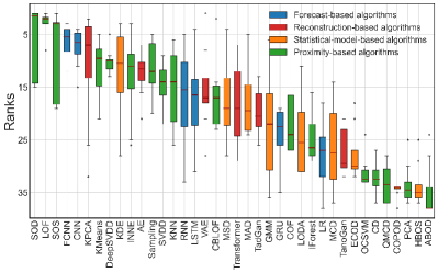
(a) Algorithms ranks under eight representative accuracy evaluation measures when KNC$<$1

(b) Algorithms ranks under eight representative accuracy evaluation measures when 1$<$KNC$<$2

(c) Algorithms ranks under eight representative accuracy evaluation measures when 2$<$KNC$<$5

(d) Algorithms ranks under eight representative accuracy evaluation measures when 5$<$KNC$<$10

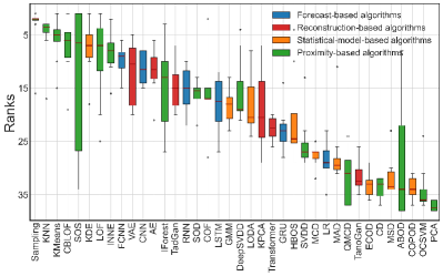
(e) Algorithms ranks under eight representative accuracy evaluation measures when 10$<$KNC

Figure 11: Performance of algorithms under eight representative accuracy evaluation measures and different KNC.

References

- Aggarwal & Sathe (2015) Aggarwal, C. C. and Sathe, S. Theoretical foundations and algorithms for outlier ensembles. Acm sigkdd explorations newsletter, 17(1):24–47, 2015.
- Back & Tsoi (1991) Back, A. D. and Tsoi, A. C. Fir and iir synapses, a new neural network architecture for time series modeling. Neural computation, 3(3):375–385, 1991.
- Bandaragoda et al. (2018) Bandaragoda, T. R., Ting, K. M., Albrecht, D., Liu, F. T., Zhu, Y., and Wells, J. R. Isolation-based anomaly detection using nearest-neighbor ensembles. Computational Intelligence, 34(4):968–998, 2018.
- Bashar & Nayak (2020) Bashar, M. A. and Nayak, R. Tanogan: Time series anomaly detection with generative adversarial networks. In 2020 IEEE Symposium Series on Computational Intelligence (SSCI), pp. 1778–1785. IEEE, 2020.
- Bhatnagar et al. (2021) Bhatnagar, A., Kassianik, P., Liu, C., Lan, T., Yang, W., Cassius, R., Sahoo, D., Arpit, D., Subramanian, S., Woo, G., et al. Merlion: A machine learning library for time series. arXiv preprint arXiv:2109.09265, 2021.
- Birgé & Rozenholc (2006) Birgé, L. and Rozenholc, Y. How many bins should be put in a regular histogram. ESAIM: Probability and Statistics, 10:24–45, 2006.
- Box & Jenkins (1976) Box, G. E. and Jenkins, G. M. Time series analysis forecasting and control-rev. 1976.
- Braei & Wagner (2020) Braei, M. and Wagner, S. Anomaly detection in univariate time-series: A survey on the state-of-the-art. arXiv preprint arXiv:2004.00433, 2020.
- Breunig et al. (2000) Breunig, M. M., Kriegel, H.-P., Ng, R. T., and Sander, J. Lof: identifying density-based local outliers. In Proceedings of the 2000 ACM SIGMOD international conference on Management of data, pp. 93–104, 2000.
- Chang et al. (1988) Chang, I., Tiao, G. C., and Chen, C. Estimation of time series parameters in the presence of outliers. Technometrics, 30(2):193–204, 1988.
- Chawla & Gionis (2013) Chawla, S. and Gionis, A. k-means–: A unified approach to clustering and outlier detection. In Proceedings of the 2013 SIAM international conference on data mining, pp. 189–197. SIAM, 2013.
- Chung et al. (2014) Chung, J., Gulcehre, C., Cho, K., and Bengio, Y. Empirical evaluation of gated recurrent neural networks on sequence modeling. arXiv preprint arXiv:1412.3555, 2014.
- Connor et al. (1994) Connor, J. T., Martin, R. D., and Atlas, L. E. Recurrent neural networks and robust time series prediction. IEEE transactions on neural networks, 5(2):240–254, 1994.
- Cook (1977) Cook, R. D. Detection of influential observation in linear regression. Technometrics, 19(1):15–18, 1977.
- Das et al. (2008) Das, K., Schneider, J., and Neill, D. B. Anomaly pattern detection in categorical datasets. In Proceedings of the 14th ACM SIGKDD international conference on Knowledge discovery and data mining, pp. 169–176, 2008.
- Emmott et al. (2013) Emmott, A. F., Das, S., Dietterich, T., Fern, A., and Wong, W.-K. Systematic construction of anomaly detection benchmarks from real data. In Proceedings of the ACM SIGKDD workshop on outlier detection and description, pp. 16–21, 2013.
- Fahim & Sillitti (2019) Fahim, M. and Sillitti, A. Anomaly detection, analysis and prediction techniques in iot environment: A systematic literature review. IEEE Access, 7:81664–81681, 2019.
- Fang & Ma (2001) Fang, K.-T. and Ma, C.-X. Wrap-around l2-discrepancy of random sampling, latin hypercube and uniform designs. Journal of complexity, 17(4):608–624, 2001.
- Fernando et al. (2021) Fernando, T., Gammulle, H., Denman, S., Sridharan, S., and Fookes, C. Deep learning for medical anomaly detection–a survey. ACM Computing Surveys (CSUR), 54(7):1–37, 2021.
- Fox (1972) Fox, A. J. Outliers in time series. Journal of the Royal Statistical Society Series B: Statistical Methodology, 34(3):350–363, 1972.
- Geiger et al. (2020) Geiger, A., Liu, D., Alnegheimish, S., Cuesta-Infante, A., and Veeramachaneni, K. Tadgan: Time series anomaly detection using generative adversarial networks. In 2020 IEEE International Conference on Big Data (Big Data), pp. 33–43. IEEE, 2020.
- Han et al. (2022) Han, S., Hu, X., Huang, H., Jiang, M., and Zhao, Y. Adbench: Anomaly detection benchmark. Advances in Neural Information Processing Systems, 35:32142–32159, 2022.
- He et al. (2012) He, J., Kumar, S., and Chang, S.-F. On the difficulty of nearest neighbor search. arXiv preprint arXiv:1206.6411, 2012.
- He et al. (2003) He, Z., Xu, X., and Deng, S. Discovering cluster-based local outliers. Pattern recognition letters, 24(9-10):1641–1650, 2003.
- Hearst et al. (1998) Hearst, M. A., Dumais, S. T., Osuna, E., Platt, J., and Scholkopf, B. Support vector machines. IEEE Intelligent Systems and their applications, 13(4):18–28, 1998.
- Hilal et al. (2022) Hilal, W., Gadsden, S. A., and Yawney, J. Financial fraud: a review of anomaly detection techniques and recent advances. Expert systems With applications, 193:116429, 2022.
- Himeur et al. (2021) Himeur, Y., Ghanem, K., Alsalemi, A., Bensaali, F., and Amira, A. Artificial intelligence based anomaly detection of energy consumption in buildings: A review, current trends and new perspectives. Applied Energy, 287:116601, 2021.
- Hochreiter & Schmidhuber (1997) Hochreiter, S. and Schmidhuber, J. Long short-term memory. Neural computation, 9(8):1735–1780, 1997.
- Hoffmann (2007) Hoffmann, H. Kernel pca for novelty detection. Pattern recognition, 40(3):863–874, 2007.
- Hundman et al. (2018) Hundman, K., Constantinou, V., Laporte, C., Colwell, I., and Soderstrom, T. Detecting spacecraft anomalies using lstms and nonparametric dynamic thresholding. In Proceedings of the 24th ACM SIGKDD international conference on knowledge discovery & data mining, pp. 387–395, 2018.
- Iglewicz & Hoaglin (1993) Iglewicz, B. and Hoaglin, D. C. Volume 16: how to detect and handle outliers. Quality Press, 1993.
- Imani & Keogh (2021) Imani, S. and Keogh, E. Multi-window-finder: domain agnostic window size for time series data. Proceedings of the MileTS, 21, 2021.
- Janssens et al. (2012) Janssens, J., Huszár, F., Postma, E., and van den Herik, H. Stochastic outlier selection. Tilburg centre for Creative Computing, techreport, 1:2012, 2012.
- Jesus et al. (2021) Jesus, G., Casimiro, A., and Oliveira, A. Using machine learning for dependable outlier detection in environmental monitoring systems. ACM Transactions on Cyber-Physical Systems, 5(3):1–30, 2021.
- Kaur et al. (2017) Kaur, P., Kumar, M., and Bhandari, A. A review of detection approaches for distributed denial of service attacks. Systems Science & Control Engineering, 5(1):301–320, 2017.
- Kim & Park (2020) Kim, T. and Park, C. H. Anomaly pattern detection for streaming data. Expert Systems with Applications, 149:113252, 2020.
- Kingma & Welling (2013) Kingma, D. P. and Welling, M. Auto-encoding variational bayes. arXiv preprint arXiv:1312.6114, 2013.
- Kriegel et al. (2008) Kriegel, H.-P., Schubert, M., and Zimek, A. Angle-based outlier detection in high-dimensional data. In Proceedings of the 14th ACM SIGKDD international conference on Knowledge discovery and data mining, pp. 444–452, 2008.
- Kriegel et al. (2009) Kriegel, H.-P., Kröger, P., Schubert, E., and Zimek, A. Outlier detection in axis-parallel subspaces of high dimensional data. In Advances in Knowledge Discovery and Data Mining: 13th Pacific-Asia Conference, PAKDD 2009 Bangkok, Thailand, April 27-30, 2009 Proceedings 13, pp. 831–838. Springer, 2009.
- Lai et al. (2021) Lai, K.-H., Zha, D., Xu, J., Zhao, Y., Wang, G., and Hu, X. Revisiting time series outlier detection: Definitions and benchmarks. In Thirty-fifth conference on neural information processing systems datasets and benchmarks track (round 1), 2021.
- Latecki et al. (2007) Latecki, L. J., Lazarevic, A., and Pokrajac, D. Outlier detection with kernel density functions. In International Workshop on Machine Learning and Data Mining in Pattern Recognition, pp. 61–75. Springer, 2007.
- Lavin & Ahmad (2015) Lavin, A. and Ahmad, S. Evaluating real-time anomaly detection algorithms–the numenta anomaly benchmark. In 2015 IEEE 14th international conference on machine learning and applications (ICMLA), pp. 38–44. IEEE, 2015.
- Li et al. (2020) Li, Z., Zhao, Y., Botta, N., Ionescu, C., and Hu, X. Copod: copula-based outlier detection. In 2020 IEEE international conference on data mining (ICDM), pp. 1118–1123. IEEE, 2020.
- Li et al. (2022) Li, Z., Zhao, Y., Hu, X., Botta, N., Ionescu, C., and Chen, G. Ecod: Unsupervised outlier detection using empirical cumulative distribution functions. IEEE Transactions on Knowledge and Data Engineering, 2022.
- Liu et al. (2008) Liu, F. T., Ting, K. M., and Zhou, Z.-H. Isolation forest. In 2008 eighth ieee international conference on data mining, pp. 413–422. IEEE, 2008.
- Munir et al. (2018) Munir, M., Siddiqui, S. A., Dengel, A., and Ahmed, S. Deepant: A deep learning approach for unsupervised anomaly detection in time series. Ieee Access, 7:1991–2005, 2018.
- Page (1957) Page, E. On problems in which a change in a parameter occurs at an unknown point. Biometrika, 44(1/2):248–252, 1957.
- Pang et al. (2021) Pang, G., Shen, C., Cao, L., and Hengel, A. V. D. Deep learning for anomaly detection: A review. ACM computing surveys (CSUR), 54(2):1–38, 2021.
- Paparrizos et al. (2022a) Paparrizos, J., Boniol, P., Palpanas, T., Tsay, R. S., Elmore, A., and Franklin, M. J. Volume under the surface: a new accuracy evaluation measure for time-series anomaly detection. Proceedings of the VLDB Endowment, 15(11):2774–2787, 2022a.
- Paparrizos et al. (2022b) Paparrizos, J., Kang, Y., Boniol, P., Tsay, R. S., Palpanas, T., and Franklin, M. J. Tsb-uad: an end-to-end benchmark suite for univariate time-series anomaly detection. Proceedings of the VLDB Endowment, 15(8):1697–1711, 2022b.
- Park et al. (2020) Park, Y.-J., Fan, S.-K. S., and Hsu, C.-Y. A review on fault detection and process diagnostics in industrial processes. Processes, 8(9):1123, 2020.
- Pevnỳ (2016) Pevnỳ, T. Loda: Lightweight on-line detector of anomalies. Machine Learning, 102:275–304, 2016.
- Ramaswamy et al. (2000) Ramaswamy, S., Rastogi, R., and Shim, K. Efficient algorithms for mining outliers from large data sets. In Proceedings of the 2000 ACM SIGMOD international conference on Management of data, pp. 427–438, 2000.
- Rousseeuw & Driessen (1999) Rousseeuw, P. J. and Driessen, K. V. A fast algorithm for the minimum covariance determinant estimator. Technometrics, 41(3):212–223, 1999.
- Ruff et al. (2018) Ruff, L., Vandermeulen, R., Goernitz, N., Deecke, L., Siddiqui, S. A., Binder, A., Müller, E., and Kloft, M. Deep one-class classification. In International conference on machine learning, pp. 4393–4402. PMLR, 2018.
- Russo et al. (2020) Russo, S., Lürig, M., Hao, W., Matthews, B., and Villez, K. Active learning for anomaly detection in environmental data. Environmental Modelling & Software, 134:104869, 2020.
- Sakurada & Yairi (2014) Sakurada, M. and Yairi, T. Anomaly detection using autoencoders with nonlinear dimensionality reduction. In Proceedings of the MLSDA 2014 2nd workshop on machine learning for sensory data analysis, pp. 4–11, 2014.
- Schölkopf et al. (2001) Schölkopf, B., Platt, J. C., Shawe-Taylor, J., Smola, A. J., and Williamson, R. C. Estimating the support of a high-dimensional distribution. Neural computation, 13(7):1443–1471, 2001.
- Shyu et al. (2003) Shyu, M.-L., Chen, S.-C., Sarinnapakorn, K., and Chang, L. A novel anomaly detection scheme based on principal component classifier. In Proceedings of the IEEE foundations and new directions of data mining workshop, pp. 172–179. IEEE Press, 2003.
- Sugiyama & Borgwardt (2013) Sugiyama, M. and Borgwardt, K. Rapid distance-based outlier detection via sampling. Advances in neural information processing systems, 26, 2013.
- Tang et al. (2002) Tang, J., Chen, Z., Fu, A. W.-C., and Cheung, D. W. Enhancing effectiveness of outlier detections for low density patterns. In Advances in Knowledge Discovery and Data Mining: 6th Pacific-Asia Conference, PAKDD 2002 Taipei, Taiwan, May 6–8, 2002 Proceedings 6, pp. 535–548. Springer, 2002.
- Tatbul et al. (2018) Tatbul, N., Lee, T. J., Zdonik, S., Alam, M., and Gottschlich, J. Precision and recall for time series. Advances in neural information processing systems, 31, 2018.
- Tax & Duin (2004) Tax, D. M. and Duin, R. P. Support vector data description. Machine learning, 54:45–66, 2004.
- Tsay (1988) Tsay, R. S. Outliers, level shifts, and variance changes in time series. Journal of forecasting, 7(1):1–20, 1988.
- Tukey et al. (1977) Tukey, J. W. et al. Exploratory data analysis, volume 2. Reading, MA, 1977.