marginparsep has been altered.
topmargin has been altered.
marginparpush has been altered.
The page layout violates the ICML style. Please do not change the page layout, or include packages like geometry, savetrees, or fullpage, which change it for you. We’re not able to reliably undo arbitrary changes to the style. Please remove the offending package(s), or layout-changing commands and try again.


Online Uniform Risk Times Sampling: First Approximation Algorithms, Learning Augmentation with Full Confidence Interval Integration


Xueqing Liu1  Kyra Gan2  Esmaeil Keyvanshokooh3  Susan Murphy4 


footnotetext: 1Duke-NUS Medical School 2Cornell Tech 3Texas A&M 4Harvard University.  
Abstract

In digital health, the strategy of allocating a limited treatment budget across available risk times is crucial to reduce user fatigue. This strategy, however, encounters a significant obstacle due to the unknown actual number of risk times, a factor not adequately addressed by existing methods lacking theoretical guarantees. This paper introduces, for the first time, the online uniform risk times sampling problem within the approximation algorithm framework. We propose two online approximation algorithms for this problem, one with and one without learning augmentation, and provide rigorous theoretical performance guarantees for them using competitive ratio analysis. We assess the performance of our algorithms using both synthetic experiments and a real-world case study on HeartSteps mobile applications.

1 Introduction

The efficacy of digital health interventions depends not only on the content of the treatment but also on the timing and frequency of delivery. Administering interventions at inappropriate or low-risk times, such as when users are driving or asleep, can significantly increase mental burden and hinder engagement (Li et al., 2020; Nahum-Shani et al., 2018; Wen et al., 2017; McConnell et al., 2017; Mann & Robinson, 2009). Here, we define risk times as times when the patient is susceptible for a negative event, such as a relapse to smoking. Moreover, existing studies (Heckman et al., 2015; Klasnja et al., 2008; Dimitrijević et al., 1972) establish a positive correlation between excessive digital interventions and heightened user fatigue, suggesting a threshold beyond which intervention effectiveness may be compromised by excessive frequency. For example, in the Heartsteps V2 study (Spruijt-Metz et al., 2022), anti-sedentary messages are triggered when sedentary behavior is detected, and in the Sense2Stop study (Battalio et al., 2021), reminders for stress management practices are activated in response to detected stress. Both studies deliberately limit intervention frequency to address potential user burden and habituation.

A strategy, rooted in the ecological momentary assessment (EMA) literature and proven effective in mitigating user fatigue, involves allocating a fixed and limited budget for treatments delivered to the patient and delivering the treatment with a uniform distribution across all available risk times (e.g., Liao et al. 2018; Dennis et al. 2015; Rathbun et al. 2013; Scott et al. 2017a; b; Shiffman et al. 2008; Stone et al. 2007). Here, the available risk times represent risk times when the patient is available for intervention. This approach to uniform sampling offers three advantages. First, the definition of available risk times prevents the delivery of text messages at inappropriate times, lessening the user’s mental burden. Second, it introduces uncertainty in treatment delivery timings, effectively reducing user habituation (Dimitrijević et al., 1972). Third, the non-zero probability of sending interventions at any available risk time enhances the estimation of causal effects in various contexts (Liao et al., 2018). However, uniform sampling across risk times poses a significant challenge because the underlying true number of available risk times per decision period is unknown (Liao et al., 2018). That is, the problem is inherently online and stochastic, with information about the underlying risk level and the availability at each decision time being sequentially received in real time. We refer to the resulting problem as the “online uniform risk times sampling” problem.

The algorithmic development for this problem is intricately connected to the domain of online approximation algorithms. Within this field, the effectiveness of algorithms is commonly assessed using the concept of a competitive ratio. This metric compares the performance of an online algorithm to that of an offline clairvoyant benchmark, where we presume the unknown parameter is revealed to the clairvoyant in advance. Note that, in practical applications, no online algorithm can attain the same level of performance as the offline clairvoyant benchmark.

In this paper, we provide the first formulation of the online uniform risk time sampling problem within the framework of approximation algorithms. We propose a randomized approximation algorithm that enjoys robust theoretical guarantees across all problem instances or sample paths. Notably, this marks the first algorithm with theoretical guarantees for the problem of online uniform risk times sampling. Although online approximation algorithms may exhibit conservative behavior, our numerical experiments illustrate that our algorithm, on average, outperforms the naive benchmark.

Next, we extend our algorithm to the setting where a confidence interval for the true risk time is provided, potentially through a machine learning (ML) algorithm. To the best of our knowledge, this is the first learning-augmented approximation algorithm that integrates the entire confidence interval rather than a single point estimate. We conduct the competitive ratio analysis for our proposed learning-augmented approximation algorithm, demonstrating its consistency in the strong sense—optimal performance is achieved when the confidence interval width is zero—and robustness—the learning-augmented algorithm performs no worse than the non-learning augmented counterpart. We validate our theoretical results with numerical experiments.

The rest of the paper is organized as follows. We first introduce the formalization of the online uniform risk times sampling problem in Section 2. We introduce our randomized algorithm without learning augmentation in Section 3. This algorithm is segmented into three distinct cases based on the time horizon length, with a competitive ratio established for each. In Section 4, we develop a learning-augmented algorithm that integrates a prediction interval and offers theoretical justifications for its effectiveness. The efficacy of these algorithms is initially assessed through synthetic experiments, followed by their application in practical scenarios, as presented in Section 5.

1.1 Related Work

Uniform Risk Times Sampling  Existing methodologies, predominantly sourced from the EMA literature, typically address the challenges of self-report requests via mobile devices, constrained by budget and uniformity considerations to minimize user burden and accurately reflect user conditions across diverse contexts (Dennis et al., 2015; Rathbun et al., 2013; Scott et al., 2017a; b). However, these approaches do not specifically address the distribution of a limited treatment budget uniformly over available risk times, especially when the exact count of these times remains unknown. While Liao et al. (2018) have developed a heuristic algorithm targeting this issue, its effectiveness heavily relies on the accuracy of predicting the number of available risk times. Moreover, in the absence of a reliable predictor, these algorithms lack robust theoretical guarantees. Consequently, there is a pressing need for a more comprehensive theoretical analysis and understanding of this problem.

Online Optimization  The development of worst-case algorithms, processing online inputs across multiple time steps with irreversible decisions, is a key focus in existing literature (Mehta et al., 2013). Our work particularly relates to the multi-option ski-rental problem (Zhang et al., 2011; Shin et al., 2023), where the number of snowy days is unknown. This scenario presents customers with varied ski rental options, differing in cost and duration. The primary objective is to minimize costs while ensuring ski availability on each snowy day. Shin et al. (2023) introduced the first randomized approximation algorithm for the multi-option ski rental problem, achieving an e𝑒e-competitive ratio. In their algorithm, a random variable B𝐵B is introduced as a proxy for the unknown true horizon T𝑇T. Initially, B𝐵B is set to α𝛼\alpha, following a density function 1/α1𝛼1/\alpha within [1,e)1𝑒[1,e). The algorithm iteratively solves an optimization problem to identify an optimal set of rental options within budget B𝐵B, maximizing day coverage. Customers sequentially utilize the options until depletion, at which point B𝐵B is increased by a factor of e𝑒e, and the process is repeated. Our study builds upon the foundational work of Shin et al. (2023), introducing a novel randomized algorithm tailored to the non-learning augmented online uniform risk times sampling problem.

Learning-Augmented Online Algorithms  Many online algorithms now incorporate ML predictions about future behaviors to enhance their worst-case performance guarantees, as demonstrated in recent studies (Purohit et al., 2018; Bamas et al., 2020; Wei & Zhang, 2020; Jin & Ma, 2022). Typically, these algorithms are accompanied by a confidence level linked to the ML predictions. When this confidence level is high, the algorithm’s performance aligns closely with these predictions; conversely, the algorithm’s performance does not fall below the established worst-case guarantee. We note that when the quality of the point estimate is poor, most existing algorithms do not guarantee that the learning-augmented algorithm will perform better than the non-learning counterpart (Bamas et al., 2020). Notably, in practice, prediction intervals are often generated instead of point estimates (Shafer & Vovk, 2008). Our work presents the first integration of these prediction intervals into online algorithms, enabling our proposed algorithms to surpass the performance of their non-learning counterparts, even in cases where the prediction interval is wide.

2 Problem Framework

In the context of digital interventions, we define the online uniform risk times sampling problem as presented by Liao et al. (2018). Let T𝑇T denote the total number of decision points within a decision period, such as a day in the context of digital interventions. At each time t𝑡t, the algorithm observes the patient’s current risk level Rtsubscript𝑅𝑡R_{t} and the intervention availability indicator It{0,1}subscript𝐼𝑡01I_{t}\in\{0,1\},111For example, if patients are driving or sleeping at time t𝑡t, they are not available for intervention at t𝑡t. utilizing sensor data collected from wearable devices. The risk level Rtsubscript𝑅𝑡R_{t} can take K+1𝐾1K+1 possible values, where Rt=0subscript𝑅𝑡0R_{t}=0 indicates not at risk and Rt=k{1,,K}subscript𝑅𝑡𝑘1𝐾R_{t}=k\in\{1,\cdots,K\} indicates the arrival of risk level k𝑘k at time t𝑡t.222For example, the higher the risk level, the more likely the patient will experience a negative event, such as relapse to smoking. The algorithm is equipped with two actions At{0,1}subscript𝐴𝑡01A_{t}\in\{0,1\} to take at any given time t𝑡t, where At=0subscript𝐴𝑡0A_{t}=0 implies no treatment, and At=1subscript𝐴𝑡1A_{t}=1 represents sending a treatment that is thought to be effective. The distributions of intervention availabilities and risk levels are allowed to change arbitrarily across decision periods. We allow risk level distribution to change across decision periods because we anticipate that the treatment will reduce subsequent risk.

Now, within each decision period (e.g., within each day), we solve a new online uniform risk times sampling problem. At each risk level k𝑘k, let τksuperscriptsubscript𝜏𝑘\tau_{k}^{*} be the unknown true number of available decision times, defined as τk=t=1T𝟙{Rt=k,It=1}superscriptsubscript𝜏𝑘superscriptsubscript𝑡1𝑇subscript1formulae-sequencesubscript𝑅𝑡𝑘subscript𝐼𝑡1\tau_{k}^{*}=\sum_{t=1}^{T}\mathbbm{1}_{\{R_{t}=k,I_{t}=1\}}. We define pk,ik(0,1)subscript𝑝𝑘subscript𝑖𝑘01p_{k,i_{k}}\in(0,1) to be the treatment probability at risk level k[K]𝑘delimited-[]𝐾k\in[K] at time ik[τk]subscript𝑖𝑘delimited-[]superscriptsubscript𝜏𝑘i_{k}\in[\tau_{k}^{*}] when treatment is feasible. Note that the treatment probabilities are indexed by iksubscript𝑖𝑘i_{k} instead of t𝑡t, representing the iksubscript𝑖𝑘i_{k}-th time when the patient is at risk level k𝑘k and available for treatment. We preclude the possibility that pk,ik=0subscript𝑝𝑘subscript𝑖𝑘0p_{k,i_{k}}=0 or pk,ik=1subscript𝑝𝑘subscript𝑖𝑘1p_{k,i_{k}}=1 to facilitate after-study inference Boruvka et al. (2018); Zhou et al. (2023); Kallus & Zhou (2022).

The algorithm is provided with a soft budget of bksubscript𝑏𝑘b_{k}, representing the total expected number of interventions allowed to be delivered at risk level k𝑘k within each decision period. We assume τk>bksuperscriptsubscript𝜏𝑘subscript𝑏𝑘\tau_{k}^{*}>b_{k} for technical convenience, and as evident in practice Liao et al. (2018). Then at each decision time t𝑡t, if the patient is available for intervention (i.e., It=1subscript𝐼𝑡1I_{t}=1), the algorithm observes the patient’s current risk level Rt=ksubscript𝑅𝑡𝑘R_{t}=k and decides the intervention probability pk,iksubscript𝑝𝑘subscript𝑖𝑘p_{k,i_{k}}. If It=0subscript𝐼𝑡0I_{t}=0, no treatment may be given. As evident in prior work (see e.g., Liao et al. 2018; Dennis et al. 2015; Rathbun et al. 2013; Scott et al. 2017a; b; Shiffman et al. 2008; Stone et al. 2007), for every risk level k[K]𝑘delimited-[]𝐾k\in[K], the objectives of the online uniform risk times sampling problem are to 1) assign the intervention probabilities {pk,ik}ik[τk]subscriptsubscript𝑝𝑘subscript𝑖𝑘subscript𝑖𝑘delimited-[]superscriptsubscript𝜏𝑘\{p_{k,i_{k}}\}_{i_{k}\in[\tau_{k}^{*}]} as uniform as possible across available risk times at level k𝑘k, and 2) maximize the sum of intervention probabilities across available risk times while adhering to the budget constraint bksubscript𝑏𝑘b_{k}.

It is important to note that τksuperscriptsubscript𝜏𝑘\tau_{k}^{*} is stochastic and is revealed only at the end of the horizon T𝑇T, corresponding to the last decision time in the decision period. Without additional information on τksuperscriptsubscript𝜏𝑘\tau_{k}^{*}, the two objectives compete with each other. A naive solution to fulfill the first objective is to set pk,ik=bk/Tsubscript𝑝𝑘subscript𝑖𝑘subscript𝑏𝑘𝑇p_{k,i_{k}}=b_{k}/T for each risk level k𝑘k, which, however, fails to maximize the sum of intervention probabilities. Conversely, if we set pk,iksubscript𝑝𝑘subscript𝑖𝑘p_{k,i_{k}} to be a large value and keep it constant, there is a risk of depleting the budget before the end of the horizon, thus failing to achieve the uniformity objective. Therefore, the optimality of the two objectives cannot be simultaneously achieved in the absence of additional information on τksuperscriptsubscript𝜏𝑘\tau_{k}^{*}. Liao et al. (2018) provided a heuristic algorithm for online uniform risk times sampling in the presence of a point estimate of τksuperscriptsubscript𝜏𝑘\tau_{k}^{*}. The algorithm’s performance is significantly influenced by the accuracy of this forecast.

In scenarios where a precise prediction of τksuperscriptsubscript𝜏𝑘\tau_{k}^{*} is available, we expect the algorithm to perform near optimally. However, such accuracy is not always attainable. In instances lacking reliable predictions, an algorithm that maintains a robust worst-case guarantee is indispensable. Addressing this need, we introduce our algorithms designed for scenarios both with and without learning augmentation, detailed in Sections 3 and 4, respectively.

2.1 Optimization Framework: Balancing Objectives

Without additional information on τksuperscriptsubscript𝜏𝑘\tau_{k}^{*}, achieving the uniformity objective is impossible. Therefore, rather than setting uniformity as the primary objective in our optimization problem, we introduce it as a penalty term. This approach facilitates the assessment of various approximation algorithms, allowing us to evaluate their overall performance, including the achievement of uniformity, by directly comparing their objective function values.

For every risk level k[K]𝑘delimited-[]𝐾k\in[K], we aim to find a sequence of treatment probability assignments {pk,ik}ik[τk]subscriptsubscript𝑝𝑘subscript𝑖𝑘subscript𝑖𝑘delimited-[]superscriptsubscript𝜏𝑘\{p_{k,i_{k}}\}_{i_{k}\in[\tau_{k}^{*}]} that achieves the following two objectives:

  1. 1.

    Maximizes the sum of treatment probabilities across available risk times, subject to the “soft” budget bksubscript𝑏𝑘b_{k};

  2. 2.

    Penalizes changes in treatment probabilities within each risk level.

Formally, for each risk level k[K]𝑘delimited-[]𝐾k\in[K], we define the following optimization problem:

maxik=1τkpk,iksuperscriptsubscriptsubscript𝑖𝑘1superscriptsubscript𝜏𝑘subscript𝑝𝑘subscript𝑖𝑘\displaystyle\max\sum_{i_{k}=1}^{\tau_{k}^{*}}p_{k,i_{k}} 1τkln(maxik[τk]pk,ikminik[τk]pk,ik)1superscriptsubscript𝜏𝑘subscriptsubscript𝑖𝑘delimited-[]superscriptsubscript𝜏𝑘subscript𝑝𝑘subscript𝑖𝑘subscriptsubscript𝑖𝑘delimited-[]superscriptsubscript𝜏𝑘subscript𝑝𝑘subscript𝑖𝑘\displaystyle-\frac{1}{\tau_{k}^{*}}\ln\left(\frac{\max_{i_{k}\in[\tau_{k}^{*}]}p_{k,i_{k}}}{\min_{i_{k}\in[\tau_{k}^{*}]}p_{k,i_{k}}}\right)
s.t. 𝔼[ik=1τk\displaystyle\text{s.t. }\mathbb{E}\Bigg{[}\sum_{i_{k}=1}^{\tau_{k}^{*}} pk,ik]bk\displaystyle p_{k,i_{k}}\Bigg{]}\leq b_{k}
pk,iksubscript𝑝𝑘subscript𝑖𝑘\displaystyle p_{k,i_{k}} (0,1)ik[τk],formulae-sequenceabsent01for-allsubscript𝑖𝑘delimited-[]superscriptsubscript𝜏𝑘\displaystyle\in(0,1)\quad\forall i_{k}\in[\tau_{k}^{*}], (1)

where the expectation in the budget constraint is taken over the randomness in the algorithm. This budget constraint is “soft” in the sense that if we have multiple decision periods (which is the case in digital health), we should satisfy the budget constraint in expectation.

We note that in Problem (2.1), the penalty term for the uniformity objective is represented by:

1τkln(maxik[τk]pk,ikminik[τk]pk,ik).1superscriptsubscript𝜏𝑘subscriptsubscript𝑖𝑘delimited-[]superscriptsubscript𝜏𝑘subscript𝑝𝑘subscript𝑖𝑘subscriptsubscript𝑖𝑘delimited-[]superscriptsubscript𝜏𝑘subscript𝑝𝑘subscript𝑖𝑘\frac{1}{\tau_{k}^{*}}\ln\left(\frac{\max_{i_{k}\in[\tau_{k}^{*}]}p_{k,i_{k}}}{\min_{i_{k}\in[\tau_{k}^{*}]}p_{k,i_{k}}}\right). (2)

The penalty term (2) is inspired by the entropy change concept from thermodynamics Smith (1950). It has several nice properties: a) it equals to 0 if and only if {pk,ik}ik[τk]subscriptsubscript𝑝𝑘subscript𝑖𝑘subscript𝑖𝑘delimited-[]superscriptsubscript𝜏𝑘\{p_{k,i_{k}}\}_{i_{k}\in[\tau_{k}^{*}]} are identical, b) it increases with the maximum difference in {pk,ik}ik[τk]subscriptsubscript𝑝𝑘subscript𝑖𝑘subscript𝑖𝑘delimited-[]superscriptsubscript𝜏𝑘\{p_{k,i_{k}}\}_{i_{k}\in[\tau_{k}^{*}]}, and c) it tends towards infinity as the value of pk,iksubscript𝑝𝑘subscript𝑖𝑘p_{k,i_{k}} approaches to zero, penalizing scenarios where the expected budget is depleted before the horizon ends.

2.2 Offline Clairvoyant and Competitive Ratio

In the offline clairvoyant benchmark, the clairvoyant possesses knowledge of τksuperscriptsubscript𝜏𝑘\tau_{k}^{*} for all k[K]𝑘delimited-[]𝐾k\in[K]. When provided with these values, the optimal solution of Problem (2.1) is to set pk,ik=bk/τksubscript𝑝𝑘subscript𝑖𝑘subscript𝑏𝑘superscriptsubscript𝜏𝑘p_{k,i_{k}}=b_{k}/\tau_{k}^{*} for each risk level k[K]𝑘delimited-[]𝐾k\in[K]. Let OPT(τk)OPTsuperscriptsubscript𝜏𝑘\text{OPT}(\tau_{k}^{*}) represent the optimal value of the objective function,

i=1τkpk,ik1τkln(maxik[τk]pk,ikminik[τk]pk,ik),superscriptsubscript𝑖1superscriptsubscript𝜏𝑘subscript𝑝𝑘subscript𝑖𝑘1superscriptsubscript𝜏𝑘subscriptsubscript𝑖𝑘delimited-[]superscriptsubscript𝜏𝑘subscript𝑝𝑘subscript𝑖𝑘subscriptsubscript𝑖𝑘delimited-[]superscriptsubscript𝜏𝑘subscript𝑝𝑘subscript𝑖𝑘\sum_{i=1}^{\tau_{k}^{*}}p_{k,i_{k}}-\frac{1}{\tau_{k}^{*}}\ln\left(\frac{\max_{i_{k}\in[\tau_{k}^{*}]}p_{k,i_{k}}}{\min_{i_{k}\in[\tau_{k}^{*}]}p_{k,i_{k}}}\right),

in Problem (2.1) within the clairvoyant benchmark. Then, k[K],OPT(τk)=bkformulae-sequencefor-all𝑘delimited-[]𝐾OPTsuperscriptsubscript𝜏𝑘subscript𝑏𝑘\forall k\in[K],\text{OPT}(\tau_{k}^{*})=b_{k}. It is important to highlight that the offline clairvoyant benchmark serves as an upper bound on the best achievable performance for any online algorithm without knowledge of {τk}k[K]subscriptsuperscriptsubscript𝜏𝑘𝑘delimited-[]𝐾\{\tau_{k}^{*}\}_{k\in[K]}. In practice, no online algorithm can attain OPT(τk)OPTsuperscriptsubscript𝜏𝑘\text{OPT}(\tau_{k}^{*}).

Let SOLksubscriptSOL𝑘\text{SOL}_{k} be the objective value of Problem (2.1) achieved by an online algorithm at risk level k𝑘k, we say that

Definition 2.1 (γ𝛾\gamma-competitive).

An algorithm is γ𝛾\gamma-competitive if 𝔼[SOLk]γOPT(τk)𝔼delimited-[]subscriptSOL𝑘𝛾OPTsuperscriptsubscript𝜏𝑘\mathbb{E}[\text{SOL}_{k}]\geq\gamma\cdot\text{OPT}(\tau_{k}^{*}) for all k[K]𝑘delimited-[]𝐾k\in[K].

The key difficulty in solving Problem (2.1) in the online setting arises due to the unknown nature of {τk}k[K]subscriptsuperscriptsubscript𝜏𝑘𝑘delimited-[]𝐾\{\tau_{k}^{*}\}_{k\in[K]}. Inspired by the randomized algorithm proposed by Shin et al. (2023), we introduce the first approximation algorithm for the online uniform risk times sampling problem.

2.3 With Learning Augmentation

In the learning-augmented problem setting, we are additionally given prediction intervals {[Lk,Uk]}k[K]subscriptsubscript𝐿𝑘subscript𝑈𝑘𝑘delimited-[]𝐾\{[L_{k},U_{k}]\}_{k\in[K]}, each containing the unknown true τksuperscriptsubscript𝜏𝑘\tau_{k}^{*}. Here, we assume τksuperscriptsubscript𝜏𝑘\tau_{k}^{*} is contained within the prediction interval for simplicity, with our result generalizing to the cases where the prediction interval contains τksuperscriptsubscript𝜏𝑘\tau_{k}^{*} with high probability. We measure the performance of the learning-augmented algorithm by the standard consistency-robustness analysis. Specifically, an algorithm is said to be λ𝜆\lambda-consistent if it achieves 𝔼[SOLk]λOPT(τk)𝔼delimited-[]subscriptSOL𝑘𝜆OPTsuperscriptsubscript𝜏𝑘\mathbb{E}[\text{SOL}_{k}]\geq\lambda\cdot\text{OPT}(\tau_{k}^{*}) when the prediction is perfect, i.e., when Lk=Uksubscript𝐿𝑘subscript𝑈𝑘L_{k}=U_{k}, indicating a zero-length interval. Conversely, we say an algorithm is ρ𝜌\rho-robust if it satisfies 𝔼[SOLk]ρOPT(τk)𝔼delimited-[]subscriptSOL𝑘𝜌OPTsuperscriptsubscript𝜏𝑘\mathbb{E}[\text{SOL}_{k}]\geq\rho\cdot\text{OPT}(\tau_{k}^{*}) regardless of the width of the prediction interval [Lk,Uk]subscript𝐿𝑘subscript𝑈𝑘[L_{k},U_{k}] (e.g., the prediction interval might very well be [bk,T]subscript𝑏𝑘𝑇[b_{k},T]). In Section 4, we establish that our proposed learning-augmented algorithm is 111-consistent, achieving the optimal solution when the confidence interval width is zero, and the competitive ratio of our learning-augmented algorithm is no worse than that of the non-learning augmented counterpart.

3 Randomized Algorithm

Algorithm 1 Randomized Online Algorithm
1:  Input: T𝑇T, {bk}k=1Ksuperscriptsubscriptsubscript𝑏𝑘𝑘1𝐾\{b_{k}\}_{k=1}^{K}
2:  Initialize: {ik=0}k=1Ksuperscriptsubscriptsubscript𝑖𝑘0𝑘1𝐾\{i_{k}=0\}_{k=1}^{K}, {jk=1}k=1Ksuperscriptsubscriptsubscript𝑗𝑘1𝑘1𝐾\{j_{k}=1\}_{k=1}^{K}, we sample α[bk,bke]𝛼subscript𝑏𝑘subscript𝑏𝑘𝑒\alpha\in[b_{k},b_{k}e] from a distribution with p.d.f. f(α)=1/α𝑓𝛼1𝛼f(\alpha)=1/\alpha, and initialize {τ~k=α}k=1Ksuperscriptsubscriptsubscript~𝜏𝑘𝛼𝑘1𝐾\{\tilde{\tau}_{k}=\alpha\}_{k=1}^{K}
3:  for t=1,,T𝑡1𝑇t=1,...,T do
4:     On each iteration t𝑡t, a new risk level Rt=ksubscript𝑅𝑡𝑘R_{t}=k and intervention indicator, Itsubscript𝐼𝑡I_{t}, arrive.
5:     if It=1subscript𝐼𝑡1I_{t}=1 then
6:        Update ik=ik+1subscript𝑖𝑘subscript𝑖𝑘1i_{k}=i_{k}+1
7:     else
8:        No intervention and skip to the next iteration.
9:     end if
10:     Given iksubscript𝑖𝑘i_{k}, bksubscript𝑏𝑘b_{k}, τ~ksubscript~𝜏𝑘\tilde{\tau}_{k}, and T𝑇T, we calculate:
11:     Int(τ~k)={τ~kw.p.τ~kτ~kτ~kw.p.τ~kτ~k\mathrm{Int}(\tilde{\tau}_{k})=\left\{\begin{array}[]{ll}\lfloor\tilde{\tau}_{k}\rfloor&w.p.\quad\lceil\tilde{\tau}_{k}\rceil-\tilde{\tau}_{k}\\ \lceil\tilde{\tau}_{k}\rceil&w.p.\quad\tilde{\tau}_{k}-\lfloor\tilde{\tau}_{k}\rfloor\end{array}\right.
12:     if Tbke𝑇subscript𝑏𝑘𝑒T\leq b_{k}e then
13:        Update parameters and set pk,iksubscript𝑝𝑘subscript𝑖𝑘p_{k,i_{k}} using Subrtn. 1
14:     else if bke<Tbke2subscript𝑏𝑘𝑒𝑇subscript𝑏𝑘superscript𝑒2b_{k}e<T\leq b_{k}e^{2} then
15:        Update parameters and set pk,iksubscript𝑝𝑘subscript𝑖𝑘p_{k,i_{k}} using Subrtn. 2
16:     else
17:        Update parameters and set pk,iksubscript𝑝𝑘subscript𝑖𝑘p_{k,i_{k}} using Subrtn. 3
18:     end if
19:     Deliver treatment with probability pk,iksubscript𝑝𝑘subscript𝑖𝑘p_{k,i_{k}}
20:  end for

In this section, we introduce our randomized algorithm, Algorithm 1, designed for the online uniform risk times sampling without learning augmentation. This algorithm was inspired by the randomized algorithm proposed by Shin et al. (2023), originally devised for the multi-option ski rental problem (see detailed description in Section 1.1). Our proposed algorithm differs in the following ways:

  • In the multi-option ski rental problem, there is a single decision period, and thus there is no upper bound on the length of the horizon. In contrast, in our problem, the decision periods are repeated over time, and each decision period has the same fixed length T𝑇T.

  • The randomness in Shin et al. (2023) is introduced through an artificial variable “budget”, acting as a proxy for the number of snow days. Whereas in our problem, the randomness is introduced directly through τksuperscriptsubscript𝜏𝑘\tau_{k}^{*}. Moreover, we have an explicit budget constraint that must be satisfied.

The proposed algorithm, Algorithm 1, provides a feasible solution to Problem (2.1). At its core, our algorithm assigns the treatment probabilities in a monotonically non-increasing fashion over time. To address different decision period horizons relative to the size of the budget bksubscript𝑏𝑘b_{k}, we designed specialized approximation algorithms for three possible scenarios: 1) Tbke𝑇subscript𝑏𝑘𝑒T\leq b_{k}e (Subroutine 1), 2) bke<Tbke2subscript𝑏𝑘𝑒𝑇subscript𝑏𝑘superscript𝑒2b_{k}e<T\leq b_{k}e^{2} (Subroutine 2), and 3) T>bke2𝑇subscript𝑏𝑘superscript𝑒2T>b_{k}e^{2} (Subroutine 3).

We maintain a running “guess” of τksuperscriptsubscript𝜏𝑘\tau_{k}^{*}, denoted by τ~ksubscript~𝜏𝑘\tilde{\tau}_{k}. We initialize τ~ksubscript~𝜏𝑘\tilde{\tau}_{k} to be α𝛼\alpha, where α[bk,bke]similar-to𝛼subscript𝑏𝑘subscript𝑏𝑘𝑒\alpha\sim[b_{k},b_{k}\cdot e] with density 1/α1𝛼1/\alpha, and e𝑒e represents the Euler’s number. If the current available time for risk level k𝑘k is within our running guess τ~ksubscript~𝜏𝑘\tilde{\tau}_{k}, then we do not change the current treatment assignment probability. Otherwise, we update τ~ksubscript~𝜏𝑘\tilde{\tau}_{k} as τ~k=τ~kesubscript~𝜏𝑘subscript~𝜏𝑘𝑒\tilde{\tau}_{k}=\tilde{\tau}_{k}e and update the treatment probability according to Algorithm 1, depending on the length of the horizon T𝑇T relative to bksubscript𝑏𝑘b_{k}.

Subroutine 1 (iksubscript𝑖𝑘i_{k}, bksubscript𝑏𝑘b_{k}, τ~ksubscript~𝜏𝑘\tilde{\tau}_{k}, T𝑇T, Int(τ~k)Intsubscript~𝜏𝑘\mathrm{Int}(\tilde{\tau}_{k}))
1:  if ik>Int(τ~k)subscript𝑖𝑘Intsubscript~𝜏𝑘i_{k}>\mathrm{Int}(\tilde{\tau}_{k}) then
2:     Update τ~k=τ~kesubscript~𝜏𝑘subscript~𝜏𝑘𝑒\tilde{\tau}_{k}=\tilde{\tau}_{k}e
3:  end if
4:  Set pk,ik=bkmin(T,τ~k(e1))subscript𝑝𝑘subscript𝑖𝑘subscript𝑏𝑘𝑇subscript~𝜏𝑘𝑒1p_{k,i_{k}}=\frac{b_{k}}{\min(T,\tilde{\tau}_{k}(e-1))}
Subroutine 2 (iksubscript𝑖𝑘i_{k}, bksubscript𝑏𝑘b_{k}, τ~ksubscript~𝜏𝑘\tilde{\tau}_{k}, Int(τ~k)Intsubscript~𝜏𝑘\mathrm{Int}(\tilde{\tau}_{k}))
1:  if ik>Int(τ~k)subscript𝑖𝑘Intsubscript~𝜏𝑘i_{k}>\mathrm{Int}(\tilde{\tau}_{k}) then
2:     jk=jk+1subscript𝑗𝑘subscript𝑗𝑘1j_{k}=j_{k}+1
3:     Update τ~k=τ~kesubscript~𝜏𝑘subscript~𝜏𝑘𝑒\tilde{\tau}_{k}=\tilde{\tau}_{k}e
4:  end if
5:  if jk3subscript𝑗𝑘3j_{k}\geq 3 then
6:     Set pk,ik=bkτ~kesubscript𝑝𝑘subscript𝑖𝑘subscript𝑏𝑘subscript~𝜏𝑘𝑒p_{k,i_{k}}=\frac{b_{k}}{\tilde{\tau}_{k}e}
7:  else
8:     Set pk,ik=bkτ~k(e1)subscript𝑝𝑘subscript𝑖𝑘subscript𝑏𝑘subscript~𝜏𝑘𝑒1p_{k,i_{k}}=\frac{b_{k}}{\tilde{\tau}_{k}(e-1)}
9:  end if

Subroutine 3 (iksubscript𝑖𝑘i_{k}, bksubscript𝑏𝑘b_{k}, τ~ksubscript~𝜏𝑘\tilde{\tau}_{k}, Int(τ~k)Intsubscript~𝜏𝑘\mathrm{Int}(\tilde{\tau}_{k}))
1:  if ik>Int(τ~k)subscript𝑖𝑘Intsubscript~𝜏𝑘i_{k}>\mathrm{Int}(\tilde{\tau}_{k}) then
2:     jk=jk+1subscript𝑗𝑘subscript𝑗𝑘1j_{k}=j_{k}+1
3:     Update τ~k=τ~kesubscript~𝜏𝑘subscript~𝜏𝑘𝑒\tilde{\tau}_{k}=\tilde{\tau}_{k}e
4:     if jk3subscript𝑗𝑘3j_{k}\geq 3 then
5:        Update bk=bk(11e)subscript𝑏𝑘subscript𝑏𝑘11𝑒b_{k}=b_{k}(1-\frac{1}{e})
6:     end if
7:  end if
8:  Set pk,ik=bkτ~kesubscript𝑝𝑘subscript𝑖𝑘subscript𝑏𝑘subscript~𝜏𝑘𝑒p_{k,i_{k}}=\frac{b_{k}}{\tilde{\tau}_{k}e}

We first illustrate the feasibility of our proposed solution, i.e., the treatment assignment probabilities outputted from Algorithm 1 satisfies the budget constraint in Problem (2.1):

Lemma 3.1.

The solution of Algorithm 1 always satisfies the budget constraint in expectation, where the expectation is taken over the randomness of the algorithm.

Next, we observe that due to the monotonically non-increasing nature of the treatment probabilities, the objective in Problem (2.1) simplifies to

maxik=1τkpk,ik1τkln(pk,1pk,τk).superscriptsubscriptsubscript𝑖𝑘1superscriptsubscript𝜏𝑘subscript𝑝𝑘subscript𝑖𝑘1superscriptsubscript𝜏𝑘subscript𝑝𝑘1subscript𝑝𝑘superscriptsubscript𝜏𝑘\max\sum_{i_{k}=1}^{\tau_{k}^{*}}p_{k,i_{k}}-\frac{1}{\tau_{k}^{*}}\ln\left(\frac{p_{k,1}}{p_{k,\tau_{k}^{*}}}\right). (3)

Using Equation (3), we compute the competitive ratio:

Theorem 3.2.

Algorithm 1 is 𝒳(T)𝒳𝑇\mathcal{X}(T)-competitive, where 𝒳𝒳\mathcal{X} is defined as follows:

𝒳(T):={1e(ln(e1)+1e1)ifTbke,1eifbke<Tbke2,1e1e2ifT>bke2.assign𝒳𝑇cases1𝑒𝑒11𝑒1if𝑇subscript𝑏𝑘𝑒1𝑒ifsubscript𝑏𝑘𝑒𝑇subscript𝑏𝑘superscript𝑒21𝑒1superscript𝑒2if𝑇subscript𝑏𝑘superscript𝑒2\displaystyle\mathcal{X}(T):=\left\{\begin{array}[]{ll}\frac{1}{e}\left(\ln(e-1)+\frac{1}{e-1}\right)&\text{if}\quad T\leq b_{k}e,\\ \frac{1}{e}&\text{if}\quad b_{k}e<T\leq b_{k}e^{2},\\ \frac{1}{e}-\frac{1}{e^{2}}&\text{if}\quad T>b_{k}e^{2}.\end{array}\right.

The above competitive ratio is conservative by design: it was derived by taking the worst-case over unknown τksuperscriptsubscript𝜏𝑘\tau_{k}^{*} and horizon length T𝑇T within each case. The proof of Theorem 3.2 in Appendix A.2 outlines the competitive ratio as a function of τksuperscriptsubscript𝜏𝑘\tau_{k}^{*} and T𝑇T. In addition, in Section 5 we explore the impact of varying τksuperscriptsubscript𝜏𝑘\tau_{k}^{*} while keeping the horizon length fixed, providing a numerical illustration of how the expected competitive ratio changes. We note that the expected competitive ratio, averaged over the unknown τksuperscriptsubscript𝜏𝑘\tau_{k}^{*}, is much better than our theoretical competitive ratio illustrated above. Based on our theoretical competitive ratio in Theorem 3.2, we recommend choosing the horizon length T𝑇T relative to the budget bksubscript𝑏𝑘b_{k} to be between bkesubscript𝑏𝑘𝑒b_{k}e and bke2subscript𝑏𝑘superscript𝑒2b_{k}e^{2}, which aligns with our empirical results in Section 5 (see Remark 5.1 for details).

4 Learning-Augmented Algorithm

Algorithm 2 Randomized Online Algorithm With Predictions
1:  Input: T𝑇T, {bk}k=1Ksuperscriptsubscriptsubscript𝑏𝑘𝑘1𝐾\{b_{k}\}_{k=1}^{K}, {[Lk,Uk]}k=1Ksuperscriptsubscriptsubscript𝐿𝑘subscript𝑈𝑘𝑘1𝐾\{[L_{k},U_{k}]\}_{k=1}^{K}
2:  Initialize: {ik=0}k=1Ksuperscriptsubscriptsubscript𝑖𝑘0𝑘1𝐾\{i_{k}=0\}_{k=1}^{K}, {jk=1}k=1Ksuperscriptsubscriptsubscript𝑗𝑘1𝑘1𝐾\{j_{k}=1\}_{k=1}^{K}, sample α[bk,bke]𝛼subscript𝑏𝑘subscript𝑏𝑘𝑒\alpha\in[b_{k},b_{k}e] from a distribution with p.d.f. f(α)=1/α𝑓𝛼1𝛼f(\alpha)=1/\alpha, and initialize {τ~k=α}k=1Ksuperscriptsubscriptsubscript~𝜏𝑘𝛼𝑘1𝐾\{\tilde{\tau}_{k}=\alpha\}_{k=1}^{K}
3:  for t=1,,T𝑡1𝑇t=1,...,T do
4:     On each iteration t𝑡t, new risk level Rt=ksubscript𝑅𝑡𝑘R_{t}=k and intervention indicator, Itsubscript𝐼𝑡I_{t}, arrive.
5:     if It=1subscript𝐼𝑡1I_{t}=1 then
6:        Update ik=ik+1subscript𝑖𝑘subscript𝑖𝑘1i_{k}=i_{k}+1
7:     else
8:        No intervention and skip to the next iteration.
9:     end if
10:     Given iksubscript𝑖𝑘i_{k}, bksubscript𝑏𝑘b_{k}, Lksubscript𝐿𝑘L_{k}, Uksubscript𝑈𝑘U_{k} τ~ksubscript~𝜏𝑘\tilde{\tau}_{k}, and T𝑇T, we calculate:
11:     Int(τ~k)={τ~kw.p.τ~kτ~kτ~kw.p.τ~kτ~k\mathrm{Int}(\tilde{\tau}_{k})=\left\{\begin{array}[]{ll}\lfloor\tilde{\tau}_{k}\rfloor&w.p.\quad\lceil\tilde{\tau}_{k}\rceil-\tilde{\tau}_{k}\\ \lceil\tilde{\tau}_{k}\rceil&w.p.\quad\tilde{\tau}_{k}-\lfloor\tilde{\tau}_{k}\rfloor\end{array}\right.
12:     if Ukbkesubscript𝑈𝑘subscript𝑏𝑘𝑒U_{k}\leq b_{k}e then
13:        Update parameters and set pk,iksubscript𝑝𝑘subscript𝑖𝑘p_{k,i_{k}} using Subrtn. 4
14:     else if bke<Ukbke2subscript𝑏𝑘𝑒subscript𝑈𝑘subscript𝑏𝑘superscript𝑒2b_{k}e<U_{k}\leq b_{k}e^{2} then
15:        if UkLkbk(e1)subscript𝑈𝑘subscript𝐿𝑘subscript𝑏𝑘𝑒1U_{k}-L_{k}\leq b_{k}(e-1) then
16:           Update parameters and set pk,iksubscript𝑝𝑘subscript𝑖𝑘p_{k,i_{k}} with Subrtn. 4
17:        else
18:           Update parameters and set pk,iksubscript𝑝𝑘subscript𝑖𝑘p_{k,i_{k}} with Subrtn. 2
19:        end if
20:     else
21:        if UkLkbk(e+1)subscript𝑈𝑘subscript𝐿𝑘subscript𝑏𝑘𝑒1U_{k}-L_{k}\leq b_{k}(e+1) then
22:           Update parameters and set pk,iksubscript𝑝𝑘subscript𝑖𝑘p_{k,i_{k}} with Subrtn. 5
23:        else
24:           Update parameters and set pk,iksubscript𝑝𝑘subscript𝑖𝑘p_{k,i_{k}} with Subrtn. 6
25:        end if
26:     end if
27:     Deliver treatment with probability pk,iksubscript𝑝𝑘subscript𝑖𝑘p_{k,i_{k}}
28:  end for

Subroutine 4 (iksubscript𝑖𝑘i_{k}, bksubscript𝑏𝑘b_{k}, τ~ksubscript~𝜏𝑘\tilde{\tau}_{k}, Lksubscript𝐿𝑘L_{k}, Uksubscript𝑈𝑘U_{k}, Int(τ~k)Intsubscript~𝜏𝑘\mathrm{Int}(\tilde{\tau}_{k}))
1:  if ik>Int(τ~k)+Lksubscript𝑖𝑘Intsubscript~𝜏𝑘subscript𝐿𝑘i_{k}>\mathrm{Int}(\tilde{\tau}_{k})+L_{k} then
2:     Update τ~k=τ~kesubscript~𝜏𝑘subscript~𝜏𝑘𝑒\tilde{\tau}_{k}=\tilde{\tau}_{k}e
3:  end if
4:  Set pk,ik=bkmin(Uk,τ~k+Lk)subscript𝑝𝑘subscript𝑖𝑘subscript𝑏𝑘subscript𝑈𝑘subscript~𝜏𝑘subscript𝐿𝑘p_{k,i_{k}}=\frac{b_{k}}{\min(U_{k},\tilde{\tau}_{k}+L_{k})}
Subroutine 5 (iksubscript𝑖𝑘i_{k}, bksubscript𝑏𝑘b_{k}, τ~ksubscript~𝜏𝑘\tilde{\tau}_{k}, Lksubscript𝐿𝑘L_{k}, Uksubscript𝑈𝑘U_{k}, Int(τ~k)Intsubscript~𝜏𝑘\mathrm{Int}(\tilde{\tau}_{k}))
1:  if ik>Int(τ~k)+Lksubscript𝑖𝑘Intsubscript~𝜏𝑘subscript𝐿𝑘i_{k}>\mathrm{Int}(\tilde{\tau}_{k})+L_{k} then
2:     Update τ~k=τ~kesubscript~𝜏𝑘subscript~𝜏𝑘𝑒\tilde{\tau}_{k}=\tilde{\tau}_{k}e
3:  end if
4:  Set pk,ik=bkmin(Uk,τ~ke+Lk)subscript𝑝𝑘subscript𝑖𝑘subscript𝑏𝑘subscript𝑈𝑘subscript~𝜏𝑘𝑒subscript𝐿𝑘p_{k,i_{k}}=\frac{b_{k}}{\min(U_{k},\tilde{\tau}_{k}e+L_{k})}

Subroutine 6 (iksubscript𝑖𝑘i_{k}, bksubscript𝑏𝑘b_{k}, τ~ksubscript~𝜏𝑘\tilde{\tau}_{k}, Lksubscript𝐿𝑘L_{k}, Uksubscript𝑈𝑘U_{k}, Int(τ~k)Intsubscript~𝜏𝑘\mathrm{Int}(\tilde{\tau}_{k}))
1:  if ik>Int(τ~k)+Lksubscript𝑖𝑘Intsubscript~𝜏𝑘subscript𝐿𝑘i_{k}>\mathrm{Int}(\tilde{\tau}_{k})+L_{k} then
2:     jk=jk+1subscript𝑗𝑘subscript𝑗𝑘1j_{k}=j_{k}+1
3:     if jk=2subscript𝑗𝑘2j_{k}=2 then
4:        agent updates bk=bk(1τ~k+Lkbkτ~k(e1)+Lk)subscript𝑏𝑘subscript𝑏𝑘1subscript~𝜏𝑘subscript𝐿𝑘subscript𝑏𝑘subscript~𝜏𝑘𝑒1subscript𝐿𝑘b_{k}=b_{k}(1-\frac{\tilde{\tau}_{k}+L_{k}-b_{k}}{\tilde{\tau}_{k}(e-1)+L_{k}})
5:     else
6:        agent updates bk=bk(11e)subscript𝑏𝑘subscript𝑏𝑘11𝑒b_{k}=b_{k}(1-\frac{1}{e})
7:     end if
8:     agent updates τ~k=τ~kesubscript~𝜏𝑘subscript~𝜏𝑘𝑒\tilde{\tau}_{k}=\tilde{\tau}_{k}e
9:  end if
10:  if jk=1subscript𝑗𝑘1j_{k}=1 then
11:     agent set pk,ik=bkτ~k(e1)+Lksubscript𝑝𝑘subscript𝑖𝑘subscript𝑏𝑘subscript~𝜏𝑘𝑒1subscript𝐿𝑘p_{k,i_{k}}=\frac{b_{k}}{\tilde{\tau}_{k}(e-1)+L_{k}}
12:  else
13:     agent set pk,ik=bkτ~kesubscript𝑝𝑘subscript𝑖𝑘subscript𝑏𝑘subscript~𝜏𝑘𝑒p_{k,i_{k}}=\frac{b_{k}}{\tilde{\tau}_{k}e}
14:  end if

In this section, we propose a new approximation algorithm, Algorithm 2, under the learning-augmented setting, where we are provided with prediction intervals {[Lk,Uk]}k[K]subscriptsubscript𝐿𝑘subscript𝑈𝑘𝑘delimited-[]𝐾\{[L_{k},U_{k}]\}_{k\in[K]} for each unknown τksuperscriptsubscript𝜏𝑘\tau_{k}^{*}. Our proposed Algorithm 2 builds upon the non-learning counterpart, Algorithm 1, utilizing the given prediction interval for optimization. Similar to Algorithm 1, we initialize α[bk,bke]similar-to𝛼subscript𝑏𝑘subscript𝑏𝑘𝑒\alpha\sim[b_{k},b_{k}e] with density 1/α1𝛼1/\alpha, and the current “guess” of τksuperscriptsubscript𝜏𝑘\tau_{k}^{*} is reflected by τ~k+Lksubscript~𝜏𝑘subscript𝐿𝑘\tilde{\tau}_{k}+L_{k}.

In Algorithm 2, the three scenarios differ from those in Algorithm 1. Here, the distinction is based on the relationship between the upper bound of the prediction interval, Uksubscript𝑈𝑘U_{k}, and the budget bksubscript𝑏𝑘b_{k}. The three scenarios are 1) Ukbkesubscript𝑈𝑘subscript𝑏𝑘𝑒U_{k}\leq b_{k}e (Subroutine 4), 2) bke<Ukbke2subscript𝑏𝑘𝑒subscript𝑈𝑘subscript𝑏𝑘superscript𝑒2b_{k}e<U_{k}\leq b_{k}e^{2}, further divided into 2a) UkLkbk(e1)subscript𝑈𝑘subscript𝐿𝑘subscript𝑏𝑘𝑒1U_{k}-L_{k}\leq b_{k}(e-1) (Subroutine 4), and 2b) UkLk>bk(e1)subscript𝑈𝑘subscript𝐿𝑘subscript𝑏𝑘𝑒1U_{k}-L_{k}>b_{k}(e-1) (Subroutine 2), and 3) Uk>bke2subscript𝑈𝑘subscript𝑏𝑘superscript𝑒2U_{k}>b_{k}e^{2}, further divided into 3a) UkLkbk(e+1)subscript𝑈𝑘subscript𝐿𝑘subscript𝑏𝑘𝑒1U_{k}-L_{k}\leq b_{k}(e+1) (Subroutine 5), and 3b) UkLk>bk(e+1)subscript𝑈𝑘subscript𝐿𝑘subscript𝑏𝑘𝑒1U_{k}-L_{k}>b_{k}(e+1) (Subroutine 6).

Similar to Algorithm 1, we first illustrate that Algorithm 2 produces a feasible solution to Problem (2.1):

Lemma 4.1.

The solution of Algorithm 2 always satisfies the budget constraint in expectation, where the expectation is taken over the randomness of the algorithm.

The proof of Lemma 4.1 is deferred to Appendix B.1.

Theorem 4.2.

This algorithm is 111-consistent and 𝒳(Lk,Uk)𝒳subscript𝐿𝑘subscript𝑈𝑘\mathcal{X}(L_{k},U_{k})-robust, where 𝒳(Uk)𝒳subscript𝑈𝑘\mathcal{X}(U_{k}) is defined as follows:

𝒳(Uk):={ln2+e1elne1eifUkbke,1eifbke<Ukbke2,2ln(e2e+1)ifUk>bke2.assign𝒳subscript𝑈𝑘cases2𝑒1𝑒𝑒1𝑒ifsubscript𝑈𝑘subscript𝑏𝑘𝑒1𝑒ifsubscript𝑏𝑘𝑒subscript𝑈𝑘subscript𝑏𝑘superscript𝑒22superscript𝑒2𝑒1ifsubscript𝑈𝑘subscript𝑏𝑘superscript𝑒2\displaystyle\mathcal{X}(U_{k}):=\left\{\begin{array}[]{ll}\ln 2+\frac{e-1}{e}\ln\frac{e-1}{e}&\text{if}\quad U_{k}\leq b_{k}e,\\ \frac{1}{e}&\text{if}\quad b_{k}e<U_{k}\leq b_{k}e^{2},\\ 2-\ln(e^{2}-e+1)&\text{if}\quad U_{k}>b_{k}e^{2}.\end{array}\right.

We first note that Algorithm 2 is 111-consistent, achieving the performance of the offline clairvoyant when the prediction is perfect. The proof of Theorem 4.2 in Appendix B.2 details the competitive ratio as influenced by τksuperscriptsubscript𝜏𝑘\tau_{k}^{*}, Lksubscript𝐿𝑘L_{k}, and T𝑇T. Additionally, Section 5 demonstrates how varying the prediction interval width UkLksubscript𝑈𝑘subscript𝐿𝑘U_{k}-L_{k}, while maintaining a constant τksuperscriptsubscript𝜏𝑘\tau_{k}^{*}, affects performance. Notably, when comparing Theorem 4.2 with Theorem 3.2, we observe that Algorithm 2 almost always outperforms its non-learning augmented equivalent across different interval widths. We defer the discussion of the design choice of T𝑇T relative to bksubscript𝑏𝑘b_{k} in the presence of prediction intervals to Remark 5.2.
Refer to caption
Refer to caption
Refer to caption
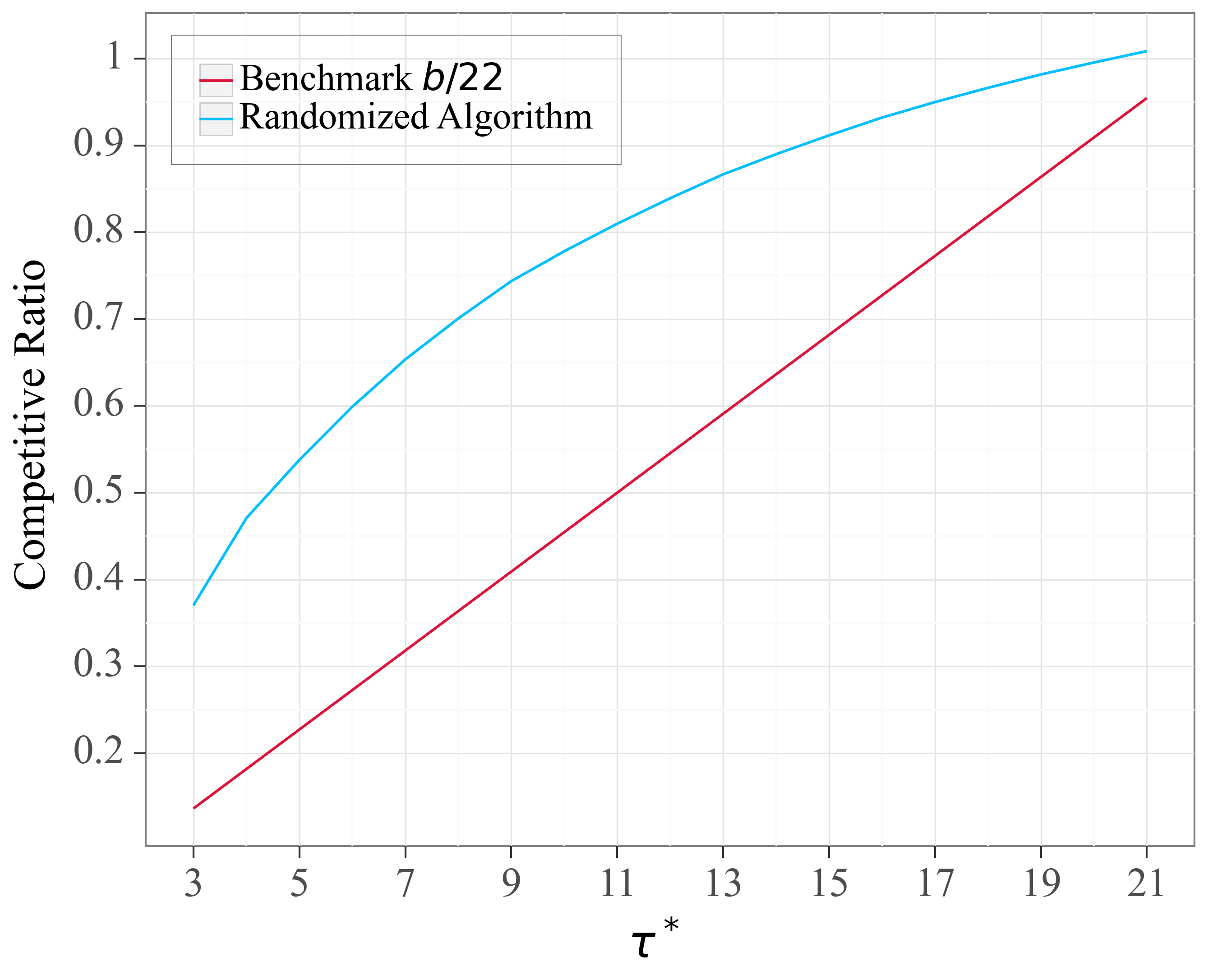
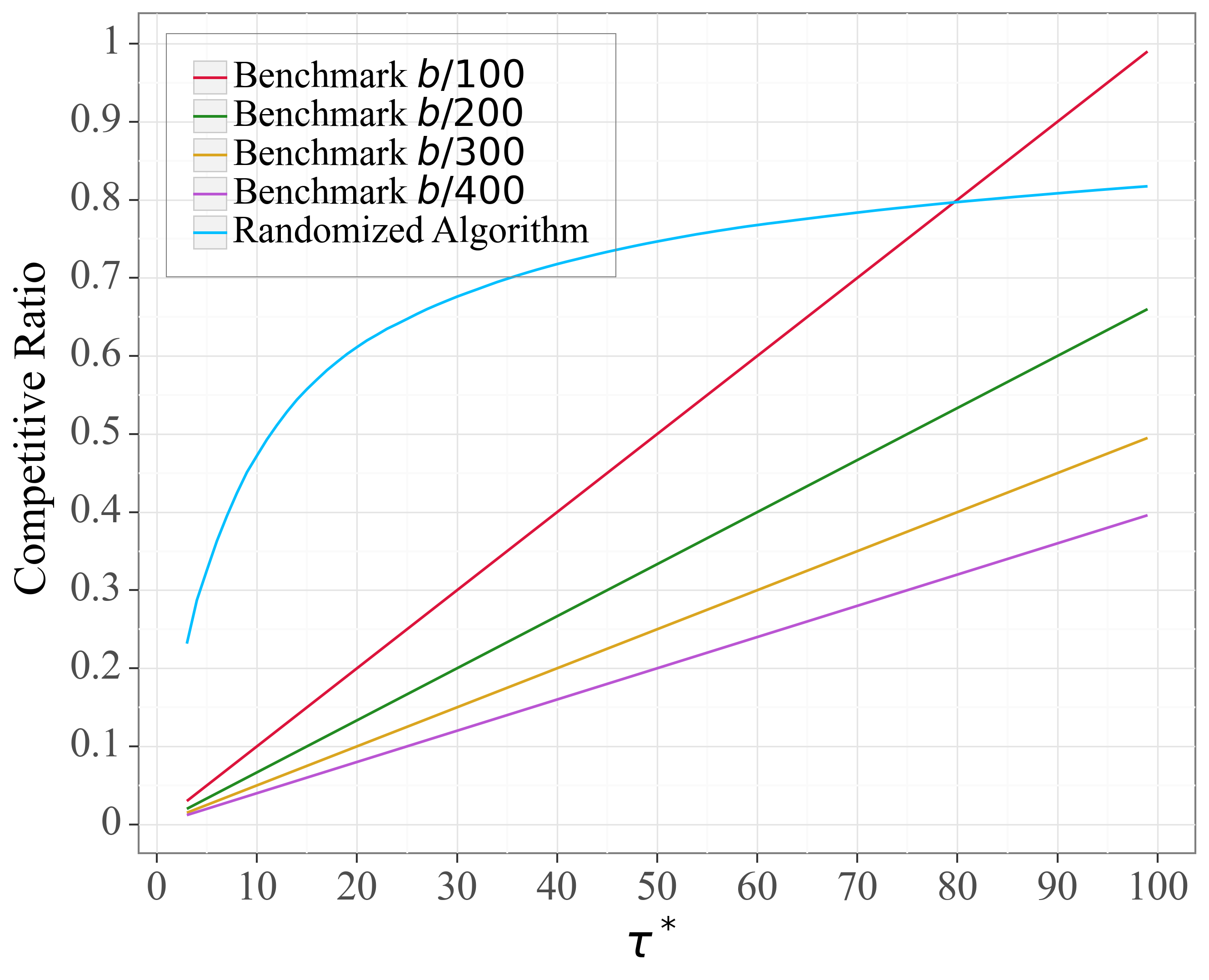
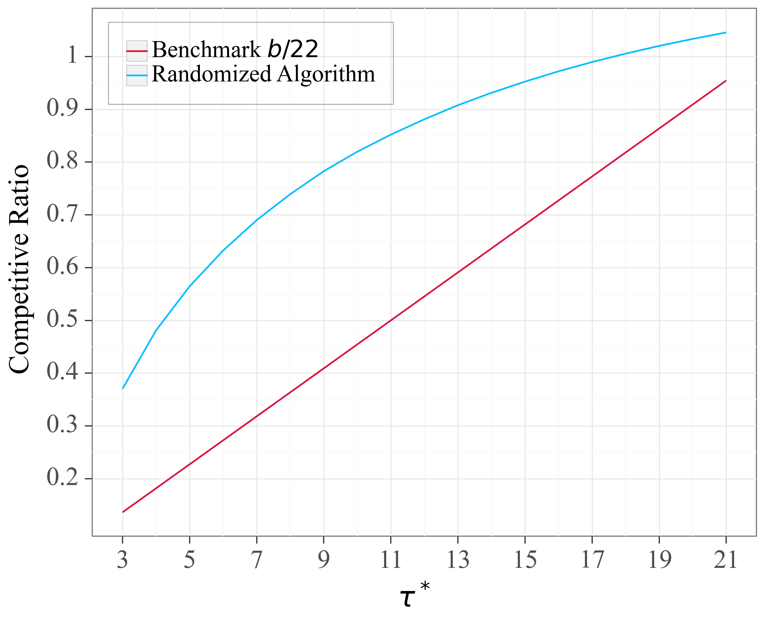
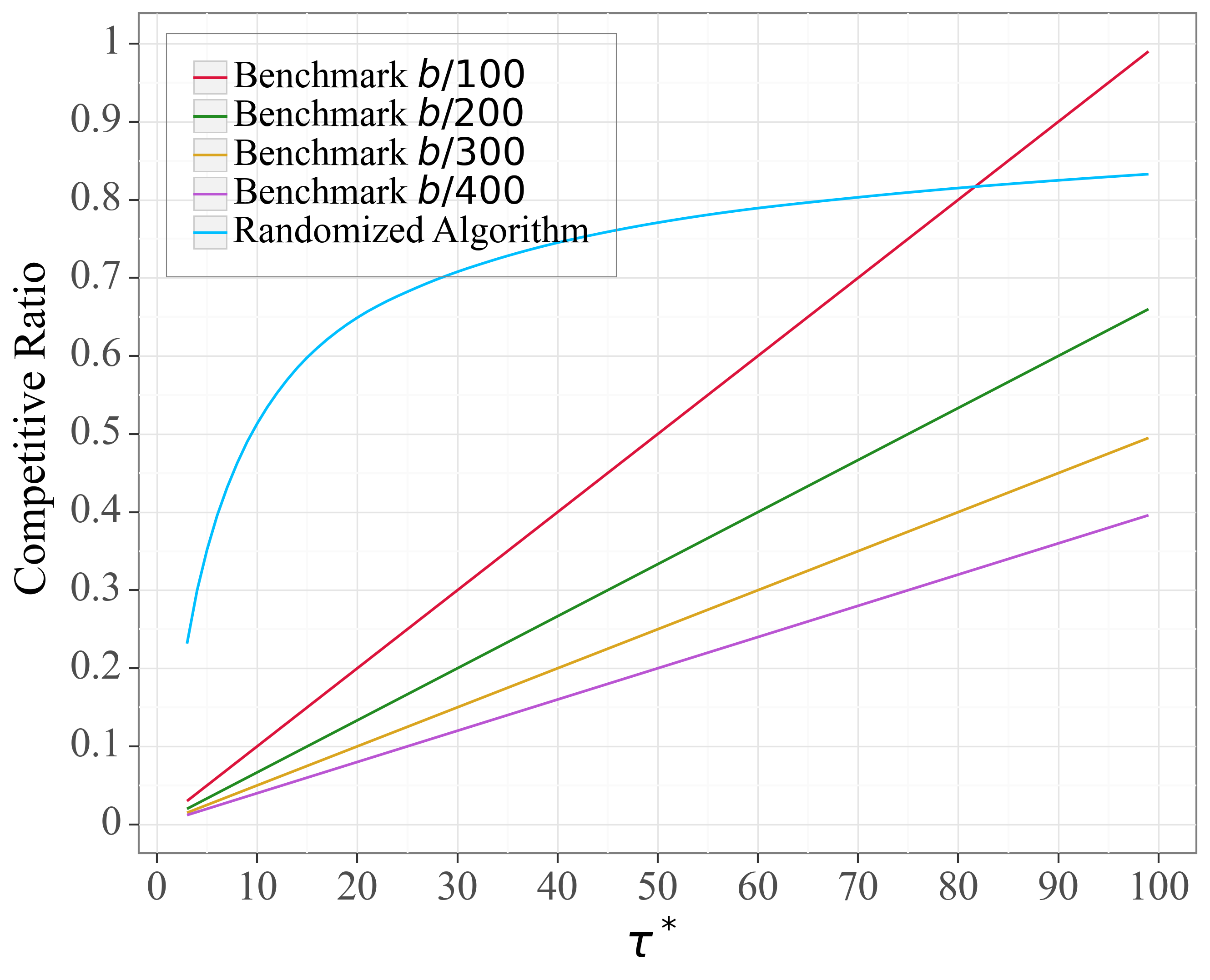
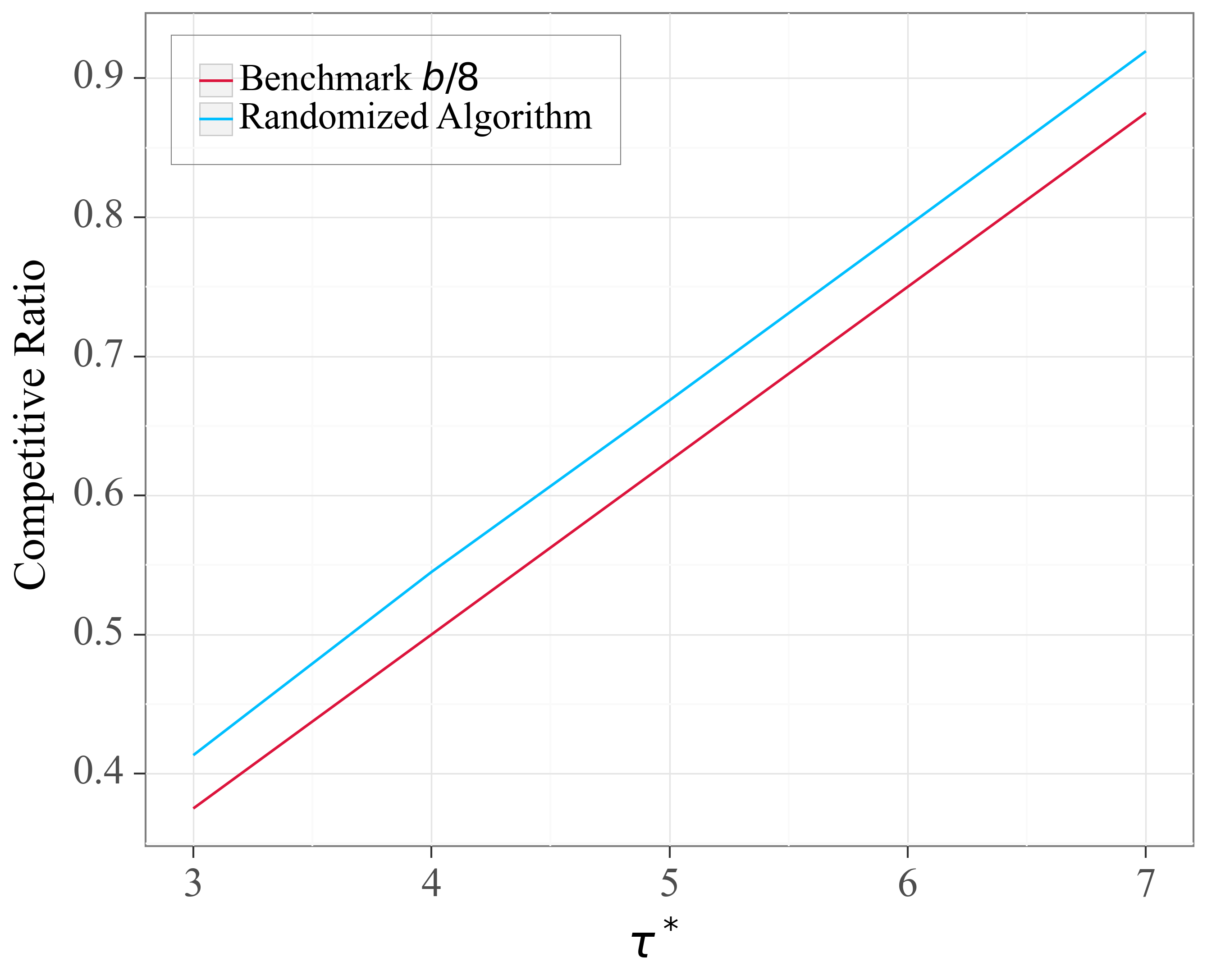
Figure 1: Average competitive ratio under non-learning augmented setting. Left: T=8𝑇8T=8; Middle: T=22𝑇22T=22; Right: T=100𝑇100T=100.

5 Experiments

In this section, we assess the performance of our proposed algorithms through numerical experiments conducted on both synthetic and real-world datasets. The metric used for evaluation is the average competitive ratio.

5.1 Synthetic Experiments

To simplify representation, we consider binary risk levels, i.e., Rt{0,1}subscript𝑅𝑡01R_{t}\in\{0,1\} with K=1𝐾1K=1, representing the patient is either at risk (Rt=1subscript𝑅𝑡1R_{t}=1) or not at risk (Rt=0subscript𝑅𝑡0R_{t}=0). In the latter case, no intervention is needed. To streamline notation, we drop the subscript k𝑘k, e.g., we use b𝑏b to represent the total expected number of interventions when the patient is at risk.

Benchmarks  In the setting without learning augmentation, we compare Algorithm 1 against a simple benchmark that achieves the uniformity objective without depleting the budget: it delivers treatments with a constant probability b/T𝑏𝑇b/T. In the learning-augmented setting, we introduce a known interval [L,U]𝐿𝑈[L,U] containing τsuperscript𝜏\tau^{*}. We compare Algorithm 2 with a benchmark that delivers interventions with a constant probability b/U𝑏𝑈b/U. In addition, we compare our learning augmented algorithm, Algorithm 2 with our non-learning augmented algorithm, Algorithm 1.

Without Learning Augmentation  In this setting, we test the performance of Algorithm 1 across all three scenarios listed in Theorem 3.2. To do this, we fix the budget level b=3𝑏3b=3, and alter the horizon lengths, T𝑇T, to correspond with each case. For Scenarios 1 and 2, we set T𝑇T to be the maximum possible length in each scenario with b=3𝑏3b=3, with T=8𝑇8T=8 and 222222 respectively in Figure 1 (left and middle). Scenario 3 in Algorithm 1 allows T𝑇T to grow to infinity asymptotically. We set T=100𝑇100T=100 for simplicity (Figure 1 right). To simulate risk occurrences, we randomly draw an integer τsuperscript𝜏\tau^{*} from the interval [b,T1]𝑏𝑇1[b,T-1] and randomly select τsuperscript𝜏\tau^{*} time points from T𝑇T, assigning Rt=1subscript𝑅𝑡1R_{t}=1 to these points. The rest are designated as Rt=0subscript𝑅𝑡0R_{t}=0.

Figure 1 shows the average competitive ratio over a range of τsuperscript𝜏\tau^{*} values. In Figure 1 (left), we observe that our randomized algorithm outperforms the benchmark by a constant competitive ratio across all values of τsuperscript𝜏\tau^{*} in Scenario 1. In Figure 1 (middle), our randomized algorithm increasingly outperforms the benchmark particularly as τsuperscript𝜏\tau^{*} deviates away from the horizon length T𝑇T in Scenario 2. We note that in Figure 1 (middle), when τ=22superscript𝜏22\tau^{*}=22, the competitive ratio slightly exceeds 1. This is attributed to our algorithm utilizing a slightly higher budget in expectation. We provide detailed insights into this observation in Appendix A.1, where we demonstrate that the worst-case budget spent is 1.044bk1.044subscript𝑏𝑘1.044b_{k}, slightly surpassing the allocated budget.

In Figure 1 (right), as T𝑇T grows, the average competitive ratio of our algorithm would remain the same as in Figure 1 (right).333This is because when b𝑏b is fixed, the treatment assignment probability is independent of T𝑇T. Here, we conclude that our algorithm increasingly outperforms the benchmark as T𝑇T grows to infinity.

Remark 5.1 (Design choice of bksubscript𝑏𝑘b_{k} and T𝑇T in absence of prediction intervals).

In real-world applications, the budget for intervention at each risk level is often fixed. Yet, there remains the design question of T𝑇T, i.e., how granular to discretize the decision period. From Figure 1, We note that although Scenario 3 yields the largest possible improvement in algorithm performance when compared with the benchmark as T𝑇T grows to infinity, our randomized algorithm has the highest competitive ratios across all τsuperscript𝜏\tau^{*} in Scenario 2. Thus, in the absence of prediction intervals, we recommend setting T𝑇T to be in between bkesubscript𝑏𝑘𝑒b_{k}e and bke2subscript𝑏𝑘superscript𝑒2b_{k}e^{2}. This recommendation changes when a prediction interval is presented.
Refer to caption
Refer to caption
Refer to caption
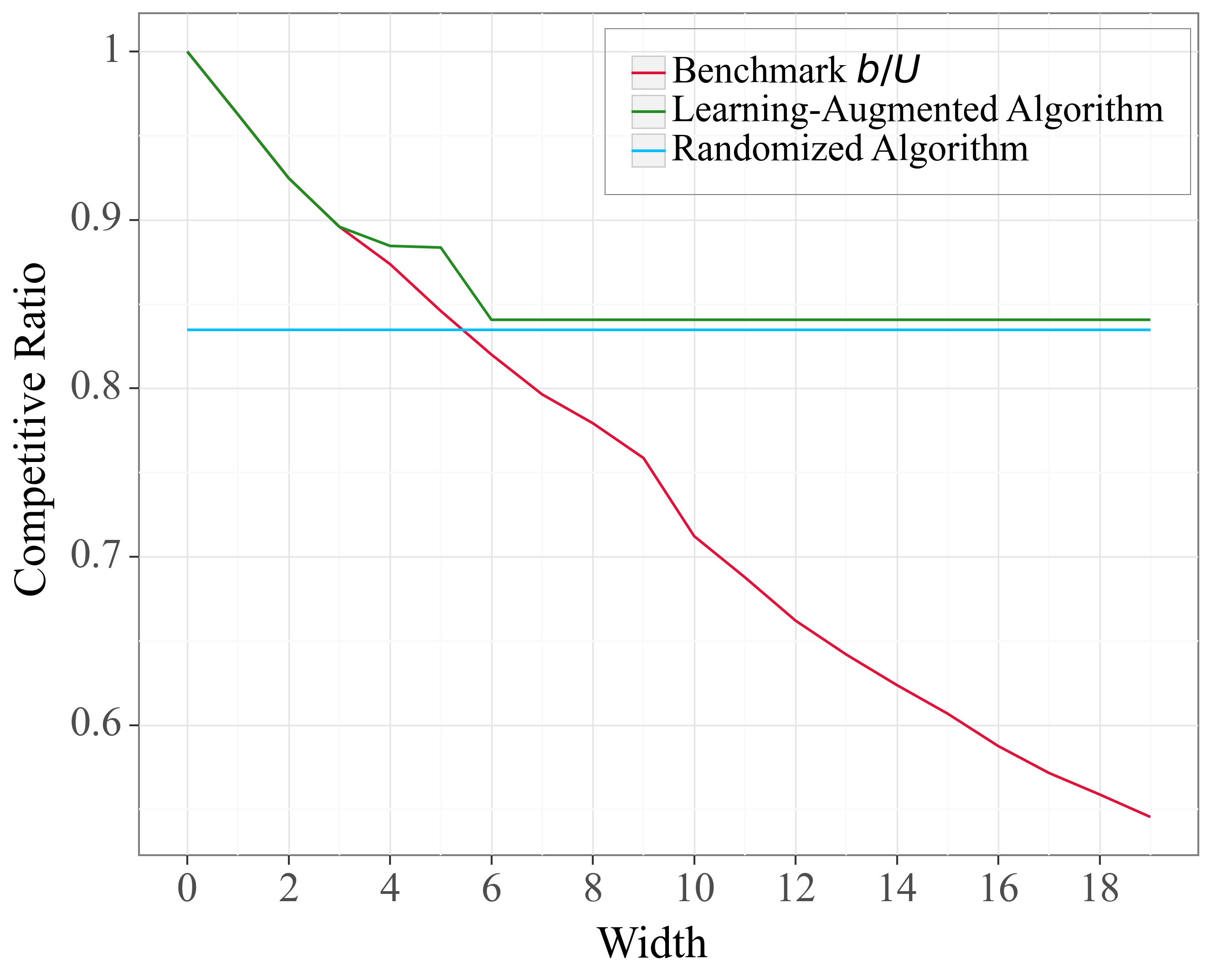
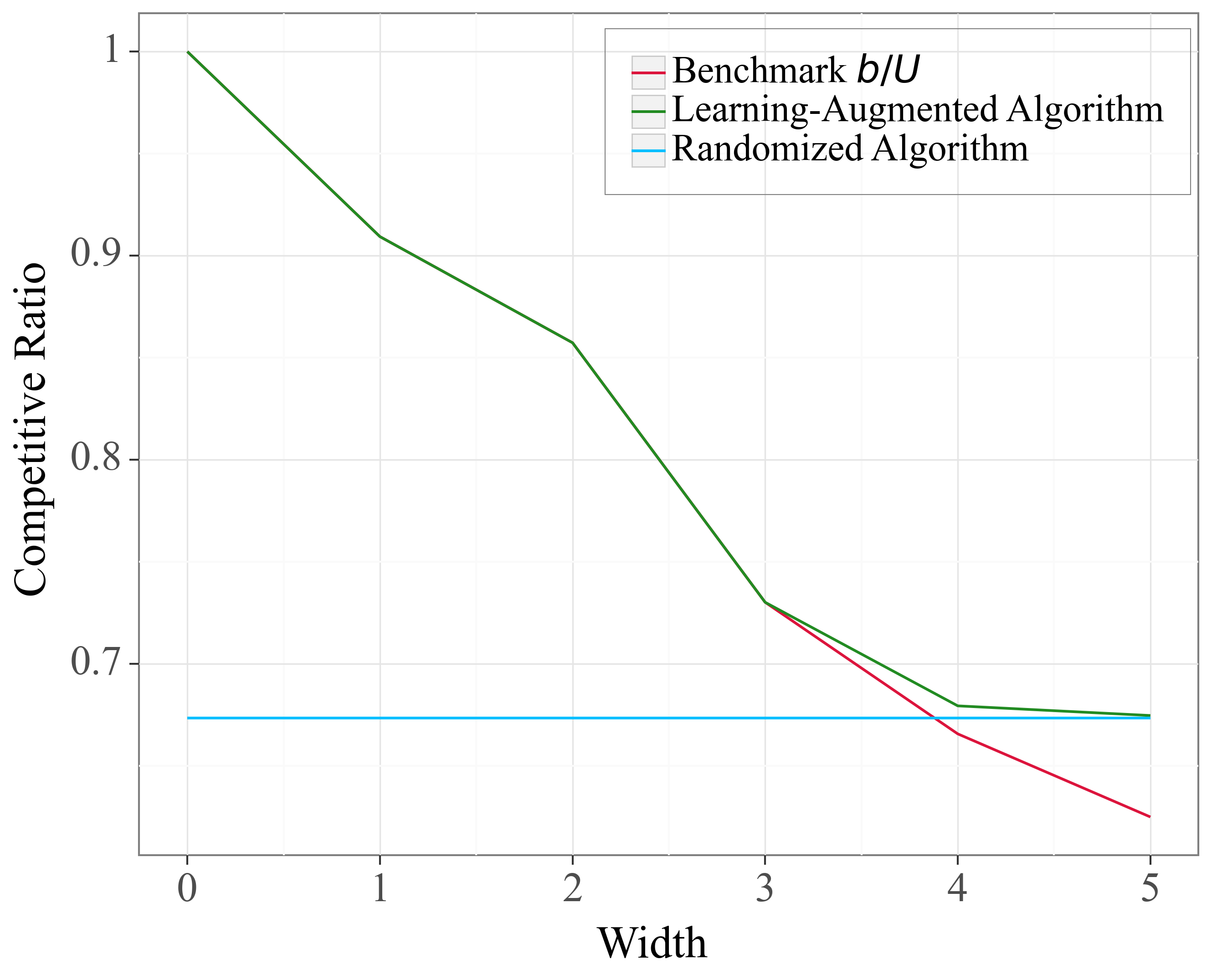
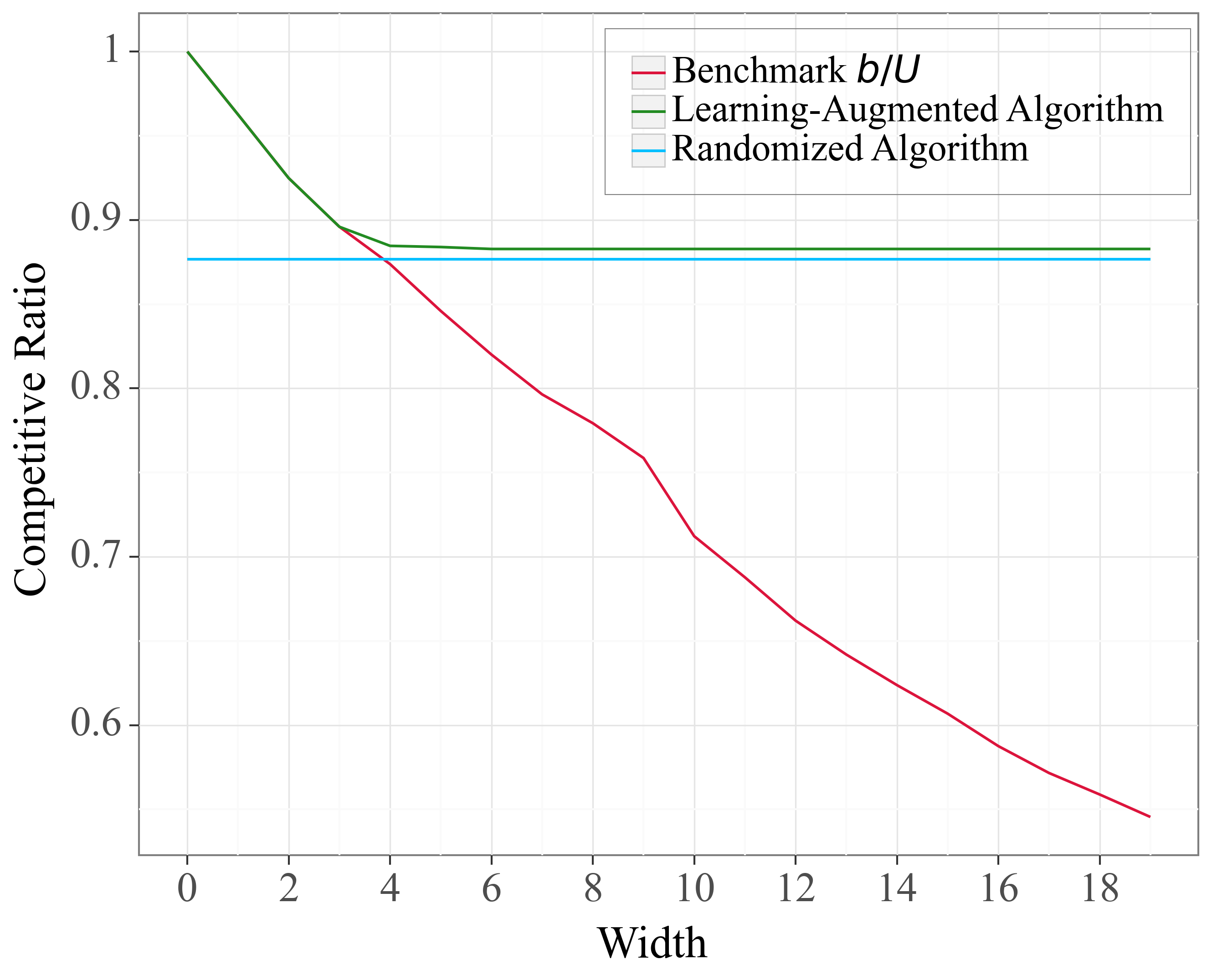
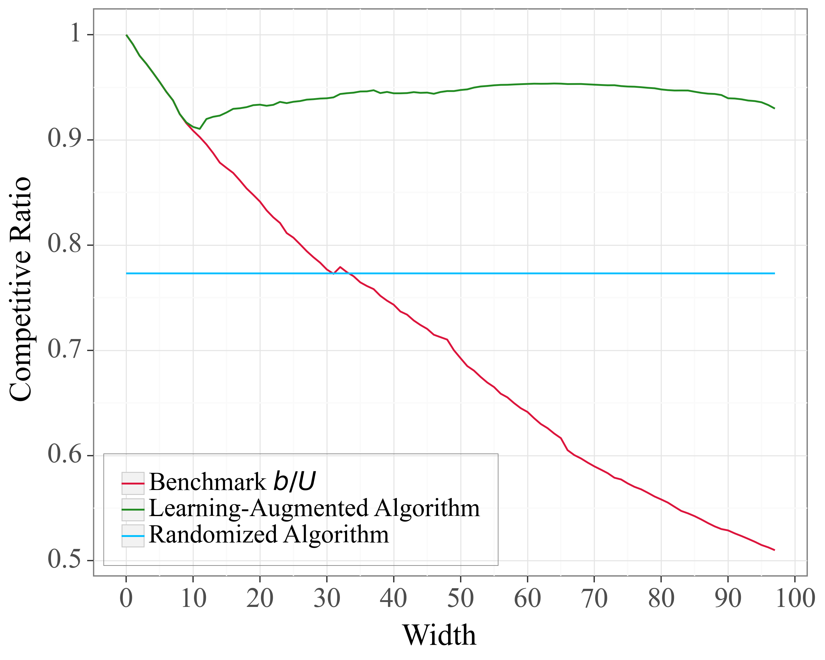
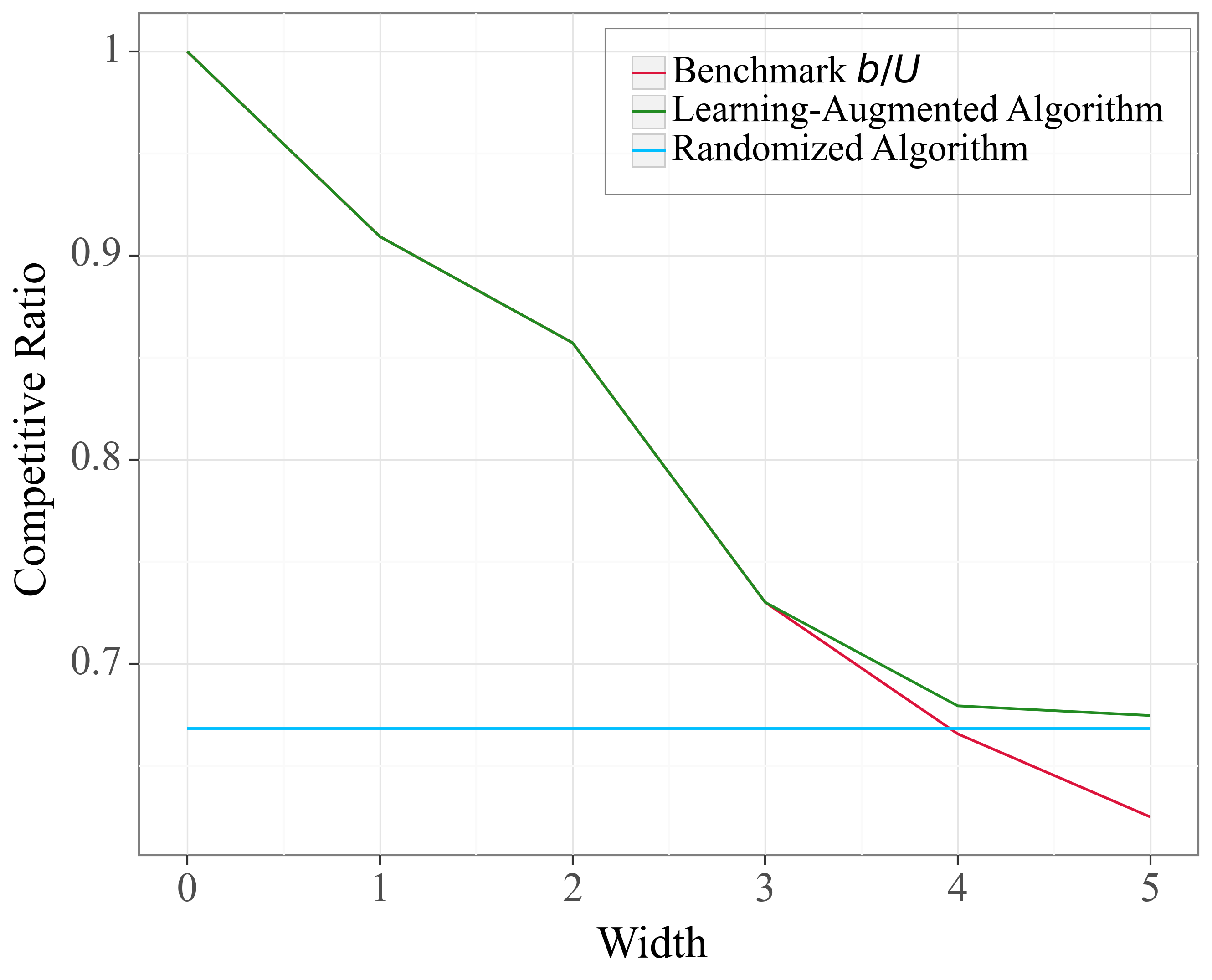
Figure 2: Average competitive ratio under learning-augmented setting. Left: T=8𝑇8T=8; Middle: T=22𝑇22T=22; Right: T=100𝑇100T=100.
Refer to caption
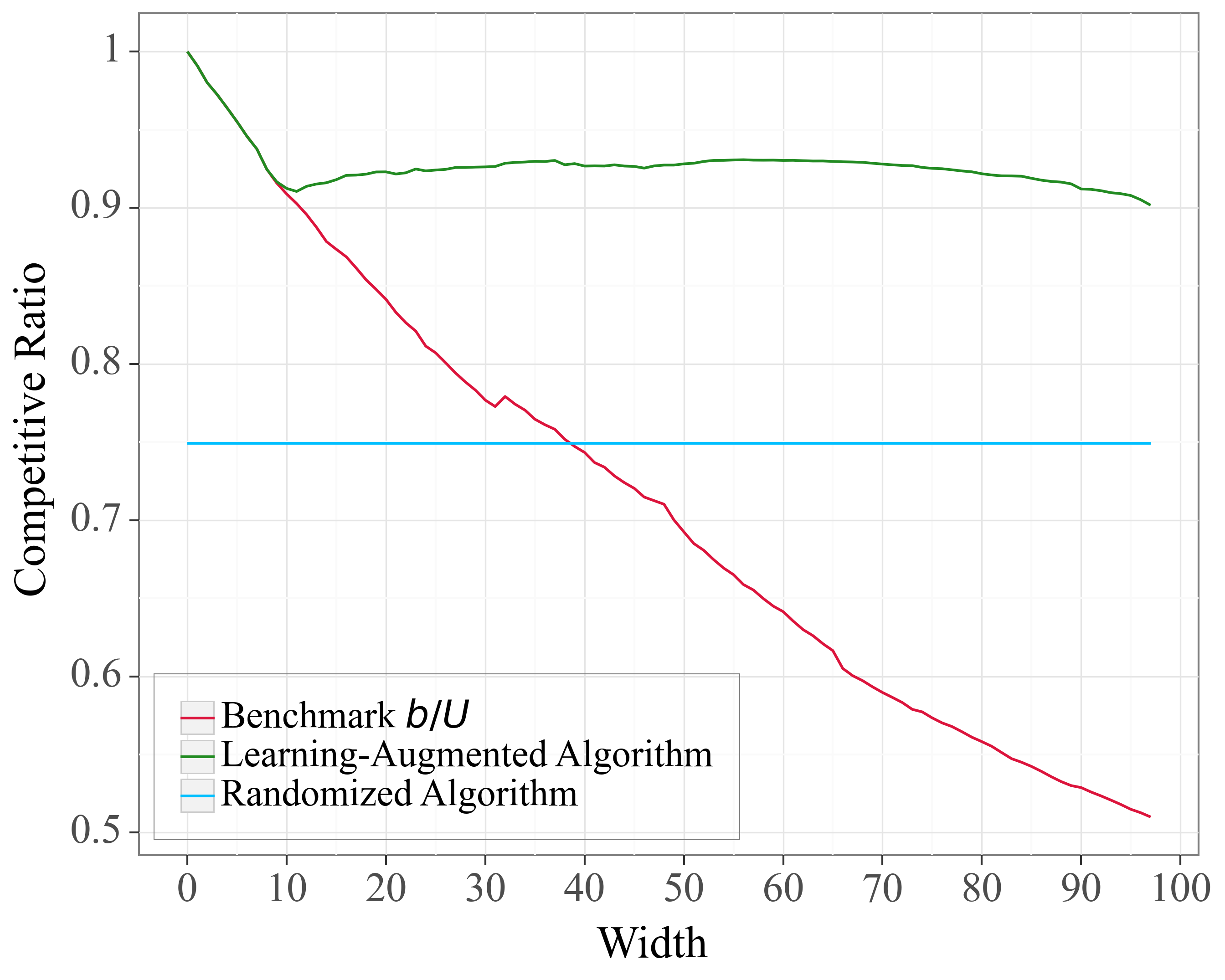
Figure 3: Average competitive ratio across user days under various prediction interval widths on HeartSteps V1 dataset. The shaded area indicates the ±1.96plus-or-minus1.96\pm 1.96 standard error bounds across user days.

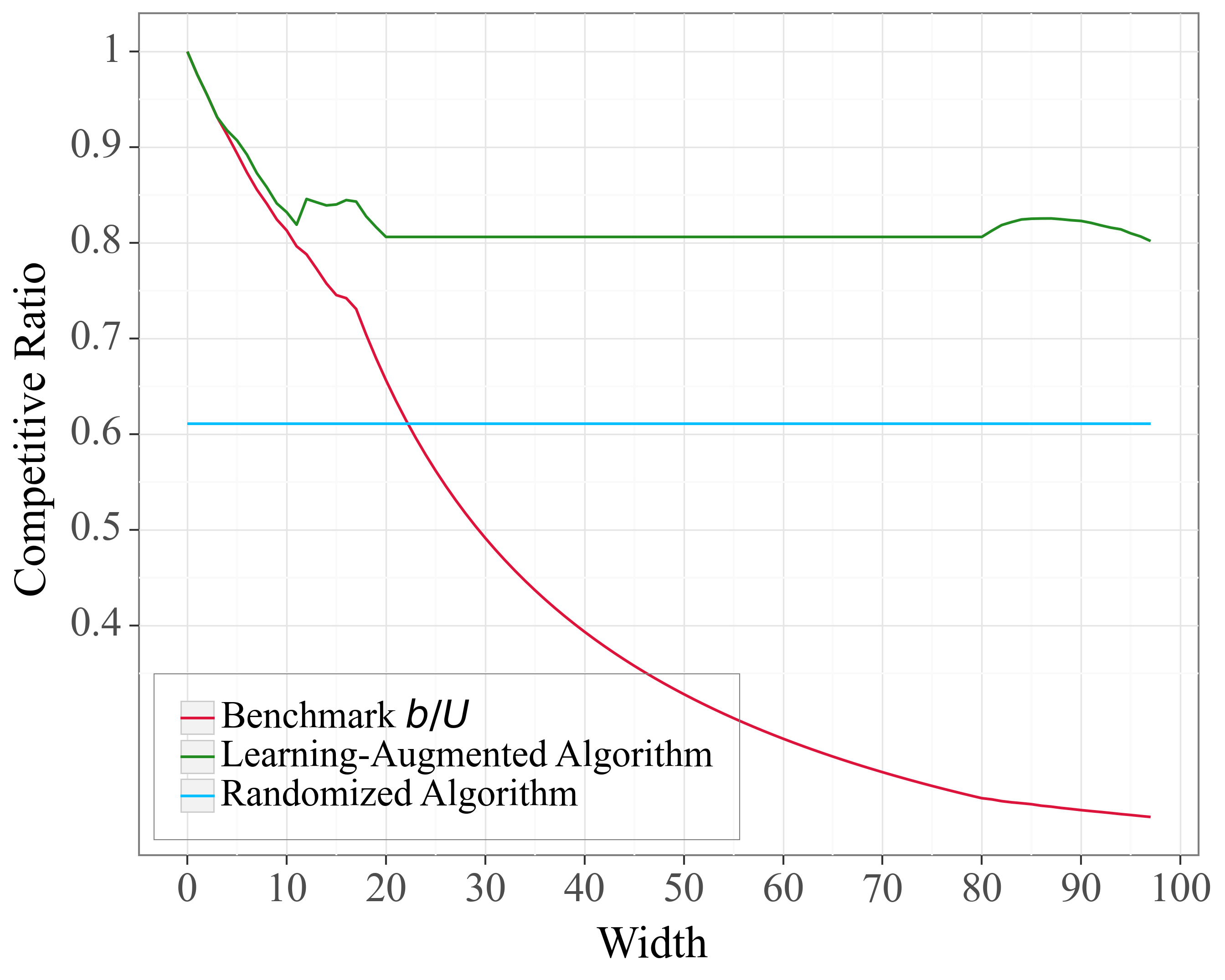
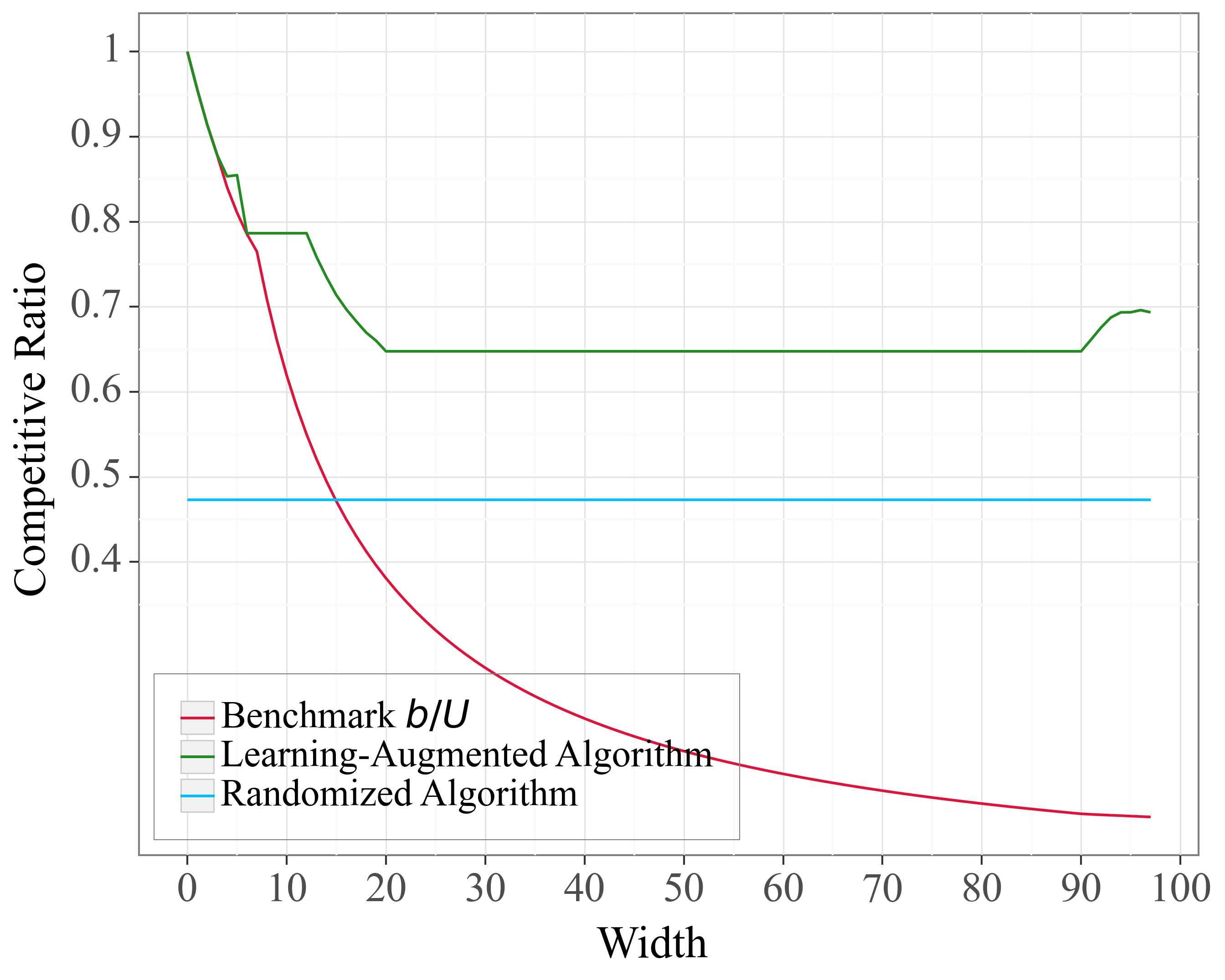
With Learning Augmentation  In this setting, we examine the performances of Algorithm 1 and Algorithm 2 under varying prediction interval widths. Similar to the non-learning augmented setting, we keep the budget fixed at b=3𝑏3b=3 and examine the performance of our learning-augmented algorithm under T=8,22,𝑇822T=8,22, and 100100100, corresponding to the three scenarios in Algorithm 2.

For enhanced comparability across various confidence widths, we maintain constant risk occurrences, τ=Int[0.5(T+b)]superscript𝜏Intdelimited-[]0.5𝑇𝑏\tau^{*}=\text{Int}[0.5(T+b)], across all simulations shown in Figure 2.444If we allow τsuperscript𝜏\tau^{*} to change across different simulations, then the difference that we observe in competitive ratio might be due to this change in τsuperscript𝜏\tau^{*}. The confidence intervals are randomly generated based on the given width, and they must contain τsuperscript𝜏\tau^{*}.

The average competitive ratio of each algorithm against a range of prediction interval widths is plotted in Figure 2. In all plots within Figure 2, we observe that the naive benchmark (where pi=b/Usubscript𝑝𝑖𝑏𝑈p_{i}=b/U for all i[τ]𝑖delimited-[]superscript𝜏i\in[\tau^{*}]) consistently outperforms the randomized algorithm (which does not have access to the prediction interval) when the confidence interval is narrow. However, as the confidence interval widens, our randomized algorithm outperforms the naive benchmark. In addition, we observe that our learning-augmented algorithm performs no worse than both the naive benchmark and the randomized algorithm. In particular, the advantage of our algorithm is the largest when in Scenario 3.

We include additional experimental results where τsuperscript𝜏\tau^{*} is small in Appendix C.1. We note that as τsuperscript𝜏\tau^{*} decreases, the advantage of our algorithm in Scenario 2 increases. In addition, we provide the competitive ratio figures in the absence of the penalization term in Problem (2.1) in Appendix C.2. This measures the fraction of the budget spent by our algorithms.

Remark 5.2 (Design choice of bksubscript𝑏𝑘b_{k} and T𝑇T in presence of prediction intervals).

In the presence of a prediction interval, if we expect the value of τsuperscript𝜏\tau^{*} to be small, we recommend setting T𝑇T to be in Scenario 2. If we expect a reasonably large value of τsuperscript𝜏\tau^{*}, we recommend setting a large value for T𝑇T such that the algorithm operates under Scenario 3.

5.2 Real-World Experiments on HeartSteps V1

Our research is inspired by the Heartsteps V1 mobile health study, which aims to enhance physical activity, specifically through regular walking, among sedentary individuals Klasnja et al. (2019). The study involved 37 participants over a follow-up period of six weeks, gathering detailed data on step counts on a minute-by-minute basis. To ensure the reliability of the step count data, our analysis was restricted to the hours from 9 am to 9 pm, with a decision time frequency set at five-minute intervals Liao et al. (2018). Consequently, this led to the accumulation of 158515851585 instances of 12-hour user-days, giving rise to a time horizon of T=144𝑇144T=144.

At each decision time point t𝑡t, we define the risk variable Rtsubscript𝑅𝑡R_{t} with a binary classification: Rt=1subscript𝑅𝑡1R_{t}=1 indicates a sedentary state, identified by recording fewer than 150 steps in the prior 40 minutes, and Rt=0subscript𝑅𝑡0R_{t}=0 signifies a non-sedentary state. Additionally, the availability for intervention, Itsubscript𝐼𝑡I_{t}, is contingent on recent messaging activity: if the user has received an anti-sedentary message within the preceding hour, Itsubscript𝐼𝑡I_{t} is set to 0; otherwise, it is set to 1. The primary objective of this strategy is to uniformly distribute around b=1.5𝑏1.5b=1.5 interventions during sedentary times each day.

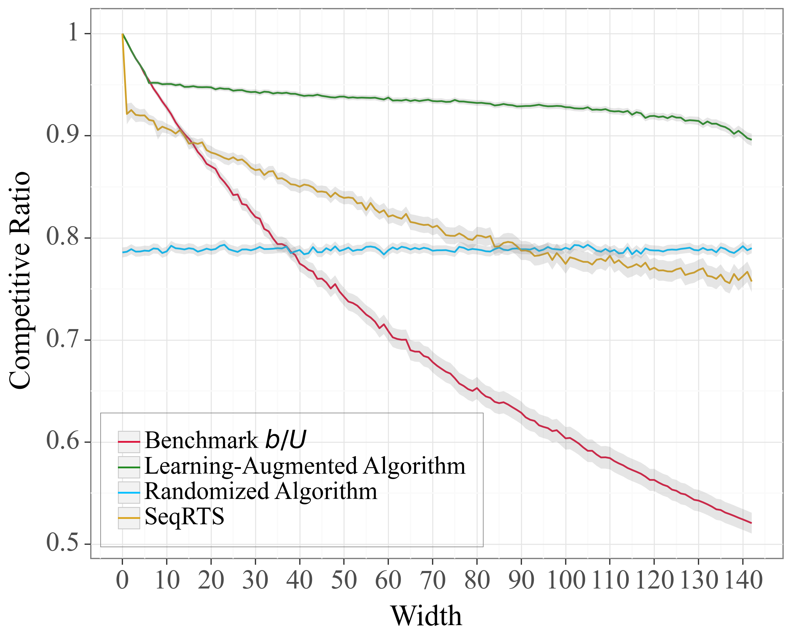
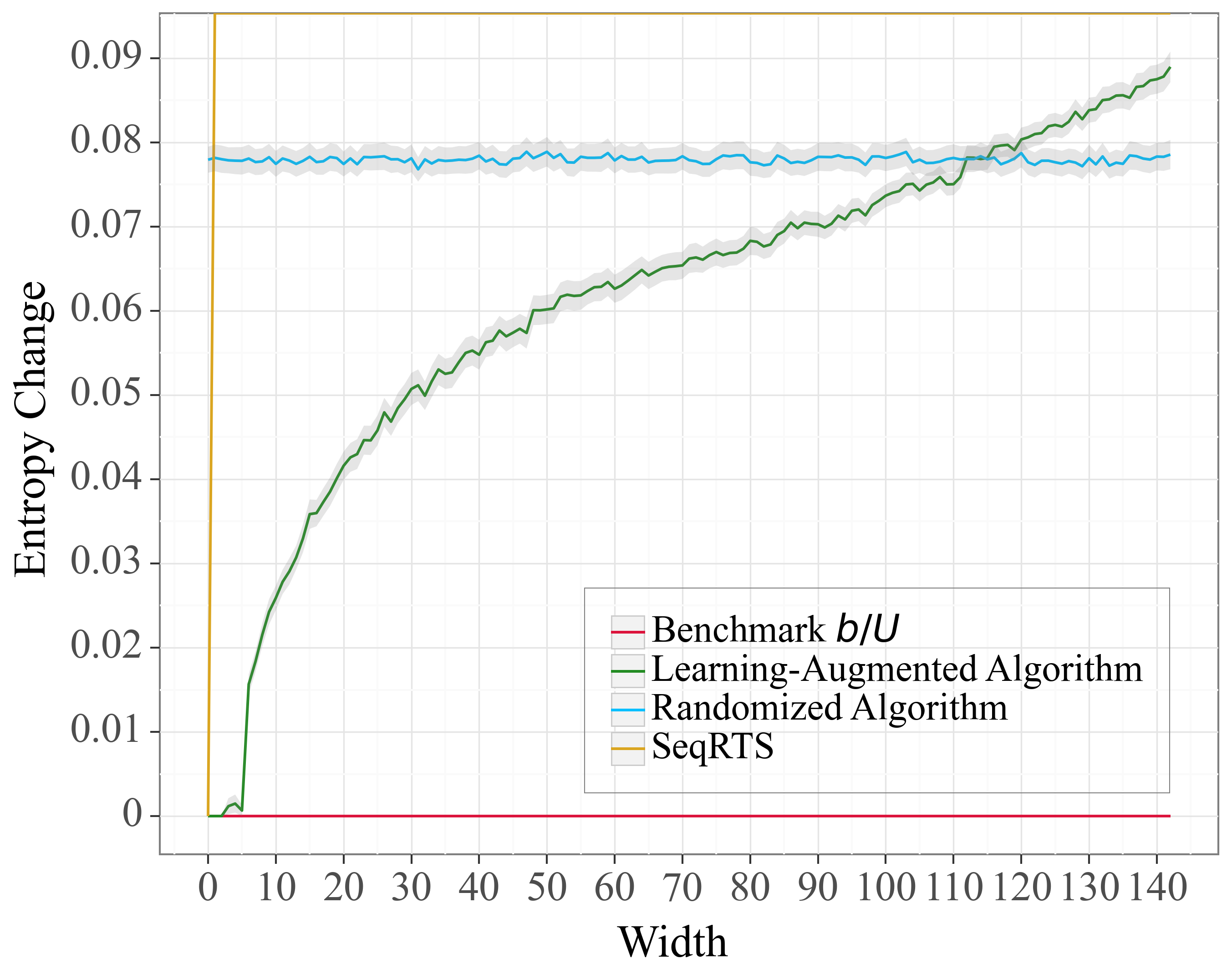
In addition to the naive benchmark bk/Usubscript𝑏𝑘𝑈b_{k}/U, our study also includes evaluations of Algorithms 1 and 2 against the SeqRTS algorithm, as introduced by Liao et al. (2018). A detailed description of the SeqRTS method is included in the Appendix D. Under SeqRTS, the budget may be depleted before allocating for all available risk times. When this happens, a minimum probability of 1×1061superscript1061\times 10^{-6} is assigned to the remaining times when calculating the objective in Problem (2.1), as illustrated in Figure 3. To better understand the behavior of SeqRTS, we set the minimum probability to 00 in Figure 8 in Appendix D. The performances are measured by competitive ratio averaged across user days.

In Figure 3, Algorithm 2, which incorporates a prediction interval, invariably outperforms the non-learning counterpart, the SeqRTS approach, and the naive benchmark bk/Usubscript𝑏𝑘𝑈b_{k}/U. Moreover, our algorithms exhibit superior uniformity in risk times sampling, evidenced by reduced entropy change compared to both the non-learning algorithm and SeqRTS, as further detailed in Figure 7 (Appendix D). Figure 8 illustrates that SeqRTS could deplete its budget even when the prediction is fairly accurate, highlighting the robustness of our algorithms under adversarial risk level arrivals. Further implementation details are included in Appendix D.

Conclusion and Future Works  This paper marks the first attempt to study the online uniform risk times sampling problem within the framework of approximation algorithms. We introduce two novel online algorithms—either incorporating learning augmentation or not—backed by rigorous theoretical guarantees and empirical results. Future works include adapting existing algorithms to scenarios where prediction intervals improve over time.

Broader Impact

The rapid advancement of digital health technologies demands innovative strategies for optimal treatment timing, specifically addressing the challenge posed by the online uniform risk times sampling problem to enhance treatment efficacy. Our research introduces online approximation algorithms augmented with ML predictions, ideally suited for scenarios where future behavior can be predicted using either real-time data accumulation or initial study results, while also ensuring the maintenance of reliable worst-case performance guarantees. Significantly, our work pioneers the integration of ML prediction intervals—widely recognized in the field—with online algorithms. This novel approach expands the applicability of a broader spectrum of ML approaches and sets a precedent for their use in diverse problem-solving contexts.

References

  • Bamas et al. (2020) Bamas, E., Maggiori, A., and Svensson, O. The primal-dual method for learning augmented algorithms. Advances in Neural Information Processing Systems, 33:20083–20094, 2020.
  • Battalio et al. (2021) Battalio, S. L., Conroy, D. E., Dempsey, W., Liao, P., Menictas, M., Murphy, S., Nahum-Shani, I., Qian, T., Kumar, S., and Spring, B. Sense2stop: a micro-randomized trial using wearable sensors to optimize a just-in-time-adaptive stress management intervention for smoking relapse prevention. Contemporary Clinical Trials, 109:106534, 2021.
  • Boruvka et al. (2018) Boruvka, A., Almirall, D., Witkiewitz, K., and Murphy, S. A. Assessing time-varying causal effect moderation in mobile health. Journal of the American Statistical Association, 113(523):1112–1121, 2018.
  • Dennis et al. (2015) Dennis, M. L., Scott, C. K., Funk, R. R., and Nicholson, L. A pilot study to examine the feasibility and potential effectiveness of using smartphones to provide recovery support for adolescents. Substance abuse, 36(4):486–492, 2015.
  • Dimitrijević et al. (1972) Dimitrijević, M. R., Faganel, J., Gregorić, M., Nathan, P., and Trontelj, J. Habituation: effects of regular and stochastic stimulation. Journal of Neurology, Neurosurgery & Psychiatry, 35(2):234–242, 1972.
  • Heckman et al. (2015) Heckman, B. W., Mathew, A. R., and Carpenter, M. J. Treatment burden and treatment fatigue as barriers to health. Current opinion in psychology, 5:31–36, 2015.
  • Jin & Ma (2022) Jin, B. and Ma, W. Online bipartite matching with advice: Tight robustness-consistency tradeoffs for the two-stage model. Advances in Neural Information Processing Systems, 35:14555–14567, 2022.
  • Kallus & Zhou (2022) Kallus, N. and Zhou, A. Stateful offline contextual policy evaluation and learning. In International Conference on Artificial Intelligence and Statistics, pp.  11169–11194. PMLR, 2022.
  • Klasnja et al. (2008) Klasnja, P., Harrison, B. L., LeGrand, L., LaMarca, A., Froehlich, J., and Hudson, S. E. Using wearable sensors and real time inference to understand human recall of routine activities. In Proceedings of the 10th international conference on Ubiquitous computing, pp.  154–163, 2008.
  • Klasnja et al. (2019) Klasnja, P., Smith, S., Seewald, N. J., Lee, A., Hall, K., Luers, B., Hekler, E. B., and Murphy, S. A. Efficacy of contextually tailored suggestions for physical activity: a micro-randomized optimization trial of heartsteps. Annals of Behavioral Medicine, 53(6):573–582, 2019.
  • Li et al. (2020) Li, S., Psihogios, A. M., McKelvey, E. R., Ahmed, A., Rabbi, M., and Murphy, S. Microrandomized trials for promoting engagement in mobile health data collection: Adolescent/young adult oral chemotherapy adherence as an example. Current opinion in systems biology, 21:1–8, 2020.
  • Liao et al. (2018) Liao, P., Dempsey, W., Sarker, H., Hossain, S. M., Al’absi, M., Klasnja, P., and Murphy, S. Just-in-Time but Not Too Much: Determining Treatment Timing in Mobile Health. Proceedings of the ACM on interactive, mobile, wearable and ubiquitous technologies, 2(4):179, December 2018. ISSN 2474-9567. doi: 10.1145/3287057.
  • Mann & Robinson (2009) Mann, S. and Robinson, A. Boredom in the lecture theatre: An investigation into the contributors, moderators and outcomes of boredom amongst university students. British Educational Research Journal, 35(2):243–258, 2009.
  • McConnell et al. (2017) McConnell, M. V., Shcherbina, A., Pavlovic, A., Homburger, J. R., Goldfeder, R. L., Waggot, D., Cho, M. K., Rosenberger, M. E., Haskell, W. L., Myers, J., et al. Feasibility of obtaining measures of lifestyle from a smartphone app: the myheart counts cardiovascular health study. JAMA cardiology, 2(1):67–76, 2017.
  • Mehta et al. (2013) Mehta, A. et al. Online matching and ad allocation. Foundations and Trends® in Theoretical Computer Science, 8(4):265–368, 2013.
  • Nahum-Shani et al. (2018) Nahum-Shani, I., Smith, S. N., Spring, B. J., Collins, L. M., Witkiewitz, K., Tewari, A., and Murphy, S. A. Just-in-time adaptive interventions (jitais) in mobile health: key components and design principles for ongoing health behavior support. Annals of Behavioral Medicine, pp.  1–17, 2018.
  • Purohit et al. (2018) Purohit, M., Svitkina, Z., and Kumar, R. Improving online algorithms via ml predictions. Advances in Neural Information Processing Systems, 31, 2018.
  • Rathbun et al. (2013) Rathbun, S. L., Song, X., Neustifter, B., and Shiffman, S. Survival analysis with time varying covariates measured at random times by design. Journal of the Royal Statistical Society Series C: Applied Statistics, 62(3):419–434, 2013.
  • Scott et al. (2017a) Scott, C. K., Dennis, M. L., Gustafson, D., and Johnson, K. A pilot study of the feasibility and potential effectiveness of using smartphones to provide recovery support. Drug and Alcohol Dependence, 100(171):e185, 2017a.
  • Scott et al. (2017b) Scott, C. K., Dennis, M. L., and Gustafson, D. H. Using smartphones to decrease substance use via self-monitoring and recovery support: study protocol for a randomized control trial. Trials, 18(1):1–11, 2017b.
  • Shafer & Vovk (2008) Shafer, G. and Vovk, V. A tutorial on conformal prediction. Journal of Machine Learning Research, 9(3), 2008.
  • Shiffman et al. (2008) Shiffman, S., Stone, A. A., and Hufford, M. R. Ecological momentary assessment. Annu. Rev. Clin. Psychol., 4:1–32, 2008.
  • Shin et al. (2023) Shin, Y., Lee, C., Lee, G., and An, H.-C. Improved learning-augmented algorithms for the multi-option ski rental problem via best-possible competitive analysis. arXiv preprint arXiv:2302.06832, 2023.
  • Smith (1950) Smith, J. M. Introduction to chemical engineering thermodynamics, 1950.
  • Spruijt-Metz et al. (2022) Spruijt-Metz, D., Marlin, B. M., Pavel, M., Rivera, D. E., Hekler, E., De La Torre, S., El Mistiri, M., Golaszweski, N. M., Li, C., Braga De Braganca, R., et al. Advancing behavioral intervention and theory development for mobile health: the heartsteps ii protocol. International journal of environmental research and public health, 19(4):2267, 2022.
  • Stone et al. (2007) Stone, A., Shiffman, S., Atienza, A., and Nebeling, L. The science of real-time data capture: Self-reports in health research. Oxford University Press, 2007.
  • Wei & Zhang (2020) Wei, A. and Zhang, F. Optimal robustness-consistency trade-offs for learning-augmented online algorithms. Advances in Neural Information Processing Systems, 33:8042–8053, 2020.
  • Wen et al. (2017) Wen, C. K. F., Schneider, S., Stone, A. A., and Spruijt-Metz, D. Compliance with mobile ecological momentary assessment protocols in children and adolescents: a systematic review and meta-analysis. Journal of medical Internet research, 19(4):e132, 2017.
  • Zhang et al. (2011) Zhang, G., Poon, C. K., and Xu, Y. The ski-rental problem with multiple discount options. Information Processing Letters, 111(18):903–906, 2011.
  • Zhou et al. (2023) Zhou, Z., Athey, S., and Wager, S. Offline multi-action policy learning: Generalization and optimization. Operations Research, 71(1):148–183, 2023.

Appendix A Proof for Algorithm 1

A.1 Proof of Lemma 3.1: Budget constraint

Proof.

We prove that the budget constraint is satisfied in expectation under each subroutine in Algorithm 1.

Subroutine 1

Recall that τksuperscriptsubscript𝜏𝑘\tau_{k}^{*} is the true number of available risk times at risk level k𝑘k. Here, we suppose τk=βejsuperscriptsubscript𝜏𝑘𝛽superscript𝑒superscript𝑗\tau_{k}^{*}=\beta e^{j^{*}} for some j+superscript𝑗superscriptj^{*}\in\mathbb{Z}^{+} and β[bk,bke]𝛽subscript𝑏𝑘subscript𝑏𝑘𝑒\beta\in[b_{k},b_{k}e]. Since Tbke𝑇subscript𝑏𝑘𝑒T\leq b_{k}e, we have that j=0superscript𝑗0j^{*}=0.

In this analysis, our focus is solely on the worst-case scenario, where both T𝑇T and τksuperscriptsubscript𝜏𝑘\tau_{k}^{*} are very close to bkesubscript𝑏𝑘𝑒b_{k}e. Assuming η>bk𝜂subscript𝑏𝑘\eta>b_{k} (where η=Te1𝜂𝑇𝑒1\eta=\frac{T}{e-1}), if this is not the case, the algorithm uniformly sets pk,ik=bkTsubscript𝑝𝑘subscript𝑖𝑘subscript𝑏𝑘𝑇p_{k,i_{k}}=\frac{b_{k}}{T} throughout.

When η>bk𝜂subscript𝑏𝑘\eta>b_{k} and α𝛼\alpha falls in the range of [bk,η]subscript𝑏𝑘𝜂[b_{k},\eta], the algorithm starts with pk,ik=bkα(e1)subscript𝑝𝑘subscript𝑖𝑘subscript𝑏𝑘𝛼𝑒1p_{k,i_{k}}=\frac{b_{k}}{\alpha(e-1)}, then transitions to pk,ik=bkTsubscript𝑝𝑘subscript𝑖𝑘subscript𝑏𝑘𝑇p_{k,i_{k}}=\frac{b_{k}}{T} for the second phase; otherwise, it consistently uses pk,ik=bkTsubscript𝑝𝑘subscript𝑖𝑘subscript𝑏𝑘𝑇p_{k,i_{k}}=\frac{b_{k}}{T}. Therefore, we have

𝔼[Budgetk]𝔼delimited-[]subscriptBudget𝑘\displaystyle\mathbb{E}[\operatorname{Budget}_{k}] =ηbkebkTβ1α𝑑α+bkη[bkα(e1)α+bkT(βα)]1α𝑑αabsentsuperscriptsubscript𝜂subscript𝑏𝑘𝑒subscript𝑏𝑘𝑇𝛽1𝛼differential-d𝛼superscriptsubscriptsubscript𝑏𝑘𝜂delimited-[]subscript𝑏𝑘𝛼𝑒1𝛼subscript𝑏𝑘𝑇𝛽𝛼1𝛼differential-d𝛼\displaystyle=\int_{\eta}^{b_{k}e}\frac{b_{k}}{T}\beta\frac{1}{\alpha}d\alpha+\int_{b_{k}}^{\eta}\Big{[}\frac{b_{k}}{\alpha(e-1)}\alpha+\frac{b_{k}}{T}(\beta-\alpha)\Big{]}\frac{1}{\alpha}d\alpha
=bkβTlnbkeη+bke1lnηbk+bkβTlnηbkbkT(ηbk)absentsubscript𝑏𝑘𝛽𝑇subscript𝑏𝑘𝑒𝜂subscript𝑏𝑘𝑒1𝜂subscript𝑏𝑘subscript𝑏𝑘𝛽𝑇𝜂subscript𝑏𝑘subscript𝑏𝑘𝑇𝜂subscript𝑏𝑘\displaystyle=\frac{b_{k}\beta}{T}\ln\frac{b_{k}e}{\eta}+\frac{b_{k}}{e-1}\ln\frac{\eta}{b_{k}}+\frac{b_{k}\beta}{T}\ln\frac{\eta}{b_{k}}-\frac{b_{k}}{T}(\eta-b_{k})
=bkβT+bke1lnηbkbkηT+bk2Tabsentsubscript𝑏𝑘𝛽𝑇subscript𝑏𝑘𝑒1𝜂subscript𝑏𝑘subscript𝑏𝑘𝜂𝑇superscriptsubscript𝑏𝑘2𝑇\displaystyle=\frac{b_{k}\beta}{T}+\frac{b_{k}}{e-1}\ln\frac{\eta}{b_{k}}-\frac{b_{k}\eta}{T}+\frac{b_{k}^{2}}{T}
bk+bke1lnTbk(e1)bke1+bk2Tincreasing withβ(β=T)absentsubscript𝑏𝑘subscript𝑏𝑘𝑒1𝑇subscript𝑏𝑘𝑒1subscript𝑏𝑘𝑒1superscriptsubscript𝑏𝑘2𝑇increasing with𝛽𝛽𝑇\displaystyle\leq b_{k}+\frac{b_{k}}{e-1}\ln\frac{T}{b_{k}(e-1)}-\frac{b_{k}}{e-1}+\frac{b_{k}^{2}}{T}\quad\text{increasing with}~{}\beta~{}(\beta=T)
bkbke1+bke1increasing withT(T=bke)absentsubscript𝑏𝑘subscript𝑏𝑘𝑒1subscript𝑏𝑘𝑒1increasing with𝑇𝑇subscript𝑏𝑘𝑒\displaystyle\leq b_{k}-\frac{b_{k}}{e-1}+\frac{b_{k}}{e-1}\quad\text{increasing with}~{}T~{}(T=b_{k}e)
bk.absentsubscript𝑏𝑘\displaystyle\leq b_{k}.

Subroutine 2

Reiterating our initial assumption, we set τk=βejsuperscriptsubscript𝜏𝑘𝛽superscript𝑒superscript𝑗\tau_{k}^{*}=\beta e^{j^{*}}. The condition bke<Tbke2subscript𝑏𝑘𝑒𝑇subscript𝑏𝑘superscript𝑒2b_{k}e<T\leq b_{k}e^{2} limits jsuperscript𝑗j^{*} to either 00 or 111. However, our analysis is particularly concerned with the worst-case scenario, hence we consider only the case where j=1superscript𝑗1j^{*}=1. The expected budget is therefore

𝔼[Budgetk]𝔼delimited-[]subscriptBudget𝑘\displaystyle\mathbb{E}\left[\operatorname{Budget}_{k}\right] =βbke[bkα(e1)α+bkαe(e1)(βeα)]1α𝑑α+bkβ[bkα(e1)α+bkαe(e1)(αeα)+bkαe3(βeαe)]1α𝑑αabsentsuperscriptsubscript𝛽subscript𝑏𝑘𝑒delimited-[]subscript𝑏𝑘𝛼𝑒1𝛼subscript𝑏𝑘𝛼𝑒𝑒1𝛽𝑒𝛼1𝛼differential-d𝛼superscriptsubscriptsubscript𝑏𝑘𝛽delimited-[]subscript𝑏𝑘𝛼𝑒1𝛼subscript𝑏𝑘𝛼𝑒𝑒1𝛼𝑒𝛼subscript𝑏𝑘𝛼superscript𝑒3𝛽𝑒𝛼𝑒1𝛼differential-d𝛼\displaystyle=\int_{\beta}^{b_{k}e}\left[\frac{b_{k}}{\alpha(e-1)}\alpha+\frac{b_{k}}{\alpha e(e-1)}(\beta e-\alpha)\right]\frac{1}{\alpha}d\alpha+\int_{b_{k}}^{\beta}\left[\frac{b_{k}}{\alpha(e-1)}\alpha+\frac{b_{k}}{\alpha e(e-1)}(\alpha e-\alpha)+\frac{b_{k}}{\alpha e^{3}}(\beta e-\alpha e)\right]\frac{1}{\alpha}d\alpha
=bke1+bkβe1(1β1bke)bke(e1)lnbkeβ+bkelnβbk+bkβe2(1bk1β)bke2lnβbkabsentsubscript𝑏𝑘𝑒1subscript𝑏𝑘𝛽𝑒11𝛽1subscript𝑏𝑘𝑒subscript𝑏𝑘𝑒𝑒1subscript𝑏𝑘𝑒𝛽subscript𝑏𝑘𝑒𝛽subscript𝑏𝑘subscript𝑏𝑘𝛽superscript𝑒21subscript𝑏𝑘1𝛽subscript𝑏𝑘superscript𝑒2𝛽subscript𝑏𝑘\displaystyle=\frac{b_{k}}{e-1}+\frac{b_{k}\beta}{e-1}(\frac{1}{\beta}-\frac{1}{b_{k}e})-\frac{b_{k}}{e(e-1)}\ln\frac{b_{k}e}{\beta}+\frac{b_{k}}{e}\ln\frac{\beta}{b_{k}}+\frac{b_{k}\beta}{e^{2}}(\frac{1}{b_{k}}-\frac{1}{\beta})-\frac{b_{k}}{e^{2}}\ln\frac{\beta}{b_{k}}
=bke1+bke1βe(e1)+βe2bke2bke(e1)+(bke+bke(e1)bke2)lnβbkabsentsubscript𝑏𝑘𝑒1subscript𝑏𝑘𝑒1𝛽𝑒𝑒1𝛽superscript𝑒2subscript𝑏𝑘superscript𝑒2subscript𝑏𝑘𝑒𝑒1subscript𝑏𝑘𝑒subscript𝑏𝑘𝑒𝑒1subscript𝑏𝑘superscript𝑒2𝛽subscript𝑏𝑘\displaystyle=\frac{b_{k}}{e-1}+\frac{b_{k}}{e-1}-\frac{\beta}{e(e-1)}+\frac{\beta}{e^{2}}-\frac{b_{k}}{e^{2}}-\frac{b_{k}}{e(e-1)}+(\frac{b_{k}}{e}+\frac{b_{k}}{e(e-1)}-\frac{b_{k}}{e^{2}})\ln\frac{\beta}{b_{k}}
=bke1+bkebke2βe2(e1)+(bke1bke2)lnβbkabsentsubscript𝑏𝑘𝑒1subscript𝑏𝑘𝑒subscript𝑏𝑘superscript𝑒2𝛽superscript𝑒2𝑒1subscript𝑏𝑘𝑒1subscript𝑏𝑘superscript𝑒2𝛽subscript𝑏𝑘\displaystyle=\frac{b_{k}}{e-1}+\frac{b_{k}}{e}-\frac{b_{k}}{e^{2}}-\frac{\beta}{e^{2}(e-1)}+(\frac{b_{k}}{e-1}-\frac{b_{k}}{e^{2}})\ln\frac{\beta}{b_{k}}
bke1+bkebke2bkee2(e1)+(bke1bke2)lnbkebkincreasing withβ(β=bke)absentsubscript𝑏𝑘𝑒1subscript𝑏𝑘𝑒subscript𝑏𝑘superscript𝑒2subscript𝑏𝑘𝑒superscript𝑒2𝑒1subscript𝑏𝑘𝑒1subscript𝑏𝑘superscript𝑒2subscript𝑏𝑘𝑒subscript𝑏𝑘increasing with𝛽𝛽subscript𝑏𝑘𝑒\displaystyle\leq\frac{b_{k}}{e-1}+\frac{b_{k}}{e}-\frac{b_{k}}{e^{2}}-\frac{b_{k}e}{e^{2}(e-1)}+(\frac{b_{k}}{e-1}-\frac{b_{k}}{e^{2}})\ln\frac{b_{k}e}{b_{k}}\quad\text{increasing with}~{}\beta~{}(\beta=b_{k}e)
=2bke+bke12bke2bkabsent2subscript𝑏𝑘𝑒subscript𝑏𝑘𝑒12subscript𝑏𝑘superscript𝑒2subscript𝑏𝑘\displaystyle=\frac{2b_{k}}{e}+\frac{b_{k}}{e-1}-\frac{2b_{k}}{e^{2}}\leq b_{k}

Subroutine 3

Under the assumption of τk=βejsuperscriptsubscript𝜏𝑘𝛽superscript𝑒superscript𝑗\tau_{k}^{*}=\beta e^{j^{*}}, and given the condition T>bke2𝑇subscript𝑏𝑘superscript𝑒2T>b_{k}e^{2}, it is possible for jsuperscript𝑗j^{*} to be 00 or to extend towards infinity. Our focus, however, is confined to the worst-case scenarios, particularly those where j1superscript𝑗1j^{*}\geq 1.

𝔼[Budgetk]𝔼delimited-[]subscriptBudget𝑘\displaystyle\mathbb{E}\left[\operatorname{Budget}_{k}\right] =βbke[bkαeα+i=2jbk(11/e)j2αej(αej1αej2)+bk(11/e)j1αej+1(βejαej1)]1α𝑑αabsentsuperscriptsubscript𝛽subscript𝑏𝑘𝑒delimited-[]subscript𝑏𝑘𝛼𝑒𝛼superscriptsubscript𝑖2superscript𝑗subscript𝑏𝑘superscript11𝑒𝑗2𝛼superscript𝑒𝑗𝛼superscript𝑒𝑗1𝛼superscript𝑒𝑗2subscript𝑏𝑘superscript11𝑒superscript𝑗1𝛼superscript𝑒superscript𝑗1𝛽superscript𝑒superscript𝑗𝛼superscript𝑒superscript𝑗11𝛼differential-d𝛼\displaystyle=\int_{\beta}^{b_{k}e}\left[\frac{b_{k}}{\alpha e}\alpha+\sum_{i=2}^{j^{*}}\frac{b_{k}(1-1/e)^{j-2}}{\alpha e^{j}}(\alpha e^{j-1}-\alpha e^{j-2})+\frac{b_{k}(1-1/e)^{j^{*}-1}}{\alpha e^{j^{*}+1}}(\beta e^{j^{*}}-\alpha e^{j^{*}-1})\right]\frac{1}{\alpha}d\alpha
+bkβ[bkαeα+j=2j+1bk(11/e)j2αej(αej1αej2)+bk(11/e)jαej+2(βejαej)]1α𝑑αsuperscriptsubscriptsubscript𝑏𝑘𝛽delimited-[]subscript𝑏𝑘𝛼𝑒𝛼superscriptsubscript𝑗2superscript𝑗1subscript𝑏𝑘superscript11𝑒𝑗2𝛼superscript𝑒𝑗𝛼superscript𝑒𝑗1𝛼superscript𝑒𝑗2subscript𝑏𝑘superscript11𝑒superscript𝑗𝛼superscript𝑒superscript𝑗2𝛽superscript𝑒superscript𝑗𝛼superscript𝑒superscript𝑗1𝛼differential-d𝛼\displaystyle\quad+\int_{b_{k}}^{\beta}\left[\frac{b_{k}}{\alpha e}\alpha+\sum_{j=2}^{j^{*}+1}\frac{b_{k}(1-1/e)^{j-2}}{\alpha e^{j}}(\alpha e^{j-1}-\alpha e^{j-2})+\frac{b_{k}(1-1/e)^{j^{*}}}{\alpha e^{j^{*}+2}}(\beta e^{j^{*}}-\alpha e^{j^{*}})\right]\frac{1}{\alpha}d\alpha
=βbke[bke+bk(11e(11e)j)+bk(e1)j1ej+1βeαα]1α𝑑αabsentsuperscriptsubscript𝛽subscript𝑏𝑘𝑒delimited-[]subscript𝑏𝑘𝑒subscript𝑏𝑘11𝑒superscript11𝑒superscript𝑗subscript𝑏𝑘superscript𝑒1superscript𝑗1superscript𝑒superscript𝑗1𝛽𝑒𝛼𝛼1𝛼differential-d𝛼\displaystyle=\int_{\beta}^{b_{k}e}\left[\frac{b_{k}}{e}+b_{k}(1-\frac{1}{e}-(1-\frac{1}{e})^{j^{*}})+\frac{b_{k}(e-1)^{j^{*}-1}}{e^{j^{*}+1}}\frac{\beta e-\alpha}{\alpha}\right]\frac{1}{\alpha}d\alpha
+bkβ[bke+bk(11e(11e)j+1)+bk(e1)jej+2βαα]1α𝑑αsuperscriptsubscriptsubscript𝑏𝑘𝛽delimited-[]subscript𝑏𝑘𝑒subscript𝑏𝑘11𝑒superscript11𝑒superscript𝑗1subscript𝑏𝑘superscript𝑒1superscript𝑗superscript𝑒superscript𝑗2𝛽𝛼𝛼1𝛼differential-d𝛼\displaystyle\quad+\int_{b_{k}}^{\beta}\left[\frac{b_{k}}{e}+b_{k}(1-\frac{1}{e}-(1-\frac{1}{e})^{j^{*}+1})+\frac{b_{k}(e-1)^{j^{*}}}{e^{j^{*}+2}}\frac{\beta-\alpha}{\alpha}\right]\frac{1}{\alpha}d\alpha
=bke+bk(11e)bk(11e)jlnbkeβbk(11e)j+1lnβbkabsentsubscript𝑏𝑘𝑒subscript𝑏𝑘11𝑒subscript𝑏𝑘superscript11𝑒superscript𝑗subscript𝑏𝑘𝑒𝛽subscript𝑏𝑘superscript11𝑒superscript𝑗1𝛽subscript𝑏𝑘\displaystyle=\frac{b_{k}}{e}+b_{k}(1-\frac{1}{e})-b_{k}(1-\frac{1}{e})^{j^{*}}\ln\frac{b_{k}e}{\beta}-b_{k}(1-\frac{1}{e})^{j^{*}+1}\ln\frac{\beta}{b_{k}}
+bk(e1)j1ej+1[eβbk+lnβbke]+bk(e1)jej+2[βbk1+lnbkβ]subscript𝑏𝑘superscript𝑒1superscript𝑗1superscript𝑒superscript𝑗1delimited-[]𝑒𝛽subscript𝑏𝑘𝛽subscript𝑏𝑘𝑒subscript𝑏𝑘superscript𝑒1superscript𝑗superscript𝑒superscript𝑗2delimited-[]𝛽subscript𝑏𝑘1subscript𝑏𝑘𝛽\displaystyle\quad+\frac{b_{k}(e-1)^{j^{*}-1}}{e^{j^{*}+1}}\left[e-\frac{\beta}{b_{k}}+\ln\frac{\beta}{b_{k}e}\right]+\frac{b_{k}(e-1)^{j^{*}}}{e^{j^{*}+2}}\left[\frac{\beta}{b_{k}}-1+\ln\frac{b_{k}}{\beta}\right]
bkbk(11e)j+1lnbkebk+bk(e1)jej+2[bkebk1+lnbkbke]increasing withβ(β=bke)absentsubscript𝑏𝑘subscript𝑏𝑘superscript11𝑒superscript𝑗1subscript𝑏𝑘𝑒subscript𝑏𝑘subscript𝑏𝑘superscript𝑒1superscript𝑗superscript𝑒superscript𝑗2delimited-[]subscript𝑏𝑘𝑒subscript𝑏𝑘1subscript𝑏𝑘subscript𝑏𝑘𝑒increasing with𝛽𝛽subscript𝑏𝑘𝑒\displaystyle\leq b_{k}-b_{k}(1-\frac{1}{e})^{j^{*}+1}\ln\frac{b_{k}e}{b_{k}}+\frac{b_{k}(e-1)^{j^{*}}}{e^{j^{*}+2}}\left[\frac{b_{k}e}{b_{k}}-1+\ln\frac{b_{k}}{b_{k}e}\right]\quad\text{increasing with}~{}\beta~{}(\beta=b_{k}e)
=bkbk(11e)j+1+bk(e1)j(e2)ej+2bkabsentsubscript𝑏𝑘subscript𝑏𝑘superscript11𝑒superscript𝑗1subscript𝑏𝑘superscript𝑒1superscript𝑗𝑒2superscript𝑒superscript𝑗2subscript𝑏𝑘\displaystyle=b_{k}-b_{k}(1-\frac{1}{e})^{j^{*}+1}+\frac{b_{k}(e-1)^{j^{*}}(e-2)}{e^{j^{*}+2}}\leq b_{k}

By combining the above results, we establish Lemma 3.1. ∎

A.2 Proof of Theorem 3.1: Competitive Ratio

Proof.

In what follows we derive the competitive ratio under each subroutine.

Subroutine 1

Recall that τksuperscriptsubscript𝜏𝑘\tau_{k}^{*} represents the actual number of available risk times at risk level k𝑘k, we assume τk=βejsuperscriptsubscript𝜏𝑘𝛽superscript𝑒superscript𝑗\tau_{k}^{*}=\beta e^{j^{*}}, where j+superscript𝑗superscriptj^{*}\in\mathbb{Z}^{+} and β[bk,bke]𝛽subscript𝑏𝑘subscript𝑏𝑘𝑒\beta\in[b_{k},b_{k}e]. It’s evident that when Tbke𝑇subscript𝑏𝑘𝑒T\leq b_{k}e, j=0superscript𝑗0j^{*}=0 follows naturally.

Defining η=T/(e1)𝜂𝑇𝑒1\eta=T/(e-1), let’s consider the case where ηbk𝜂subscript𝑏𝑘\eta\leq b_{k}, leading to Tbk(e1)𝑇subscript𝑏𝑘𝑒1T\leq b_{k}(e-1). Given that pk,ik=bkmin(T,τ~k(e1))subscript𝑝𝑘subscript𝑖𝑘subscript𝑏𝑘𝑇subscript~𝜏𝑘𝑒1p_{k,i_{k}}=\frac{b_{k}}{\min(T,\tilde{\tau}_{k}(e-1))}, it follows that the algorithm consistently sets pk,ik=bkTsubscript𝑝𝑘subscript𝑖𝑘subscript𝑏𝑘𝑇p_{k,i_{k}}=\frac{b_{k}}{T}. Consequently, we derive:

𝔼[SOLk]𝔼delimited-[]subscriptSOL𝑘\displaystyle\mathbb{E}[\operatorname{SOL}_{k}] =bkTβbkbk(e1)βbke1.absentsubscript𝑏𝑘𝑇𝛽subscript𝑏𝑘subscript𝑏𝑘𝑒1𝛽subscript𝑏𝑘𝑒1\displaystyle=\frac{b_{k}}{T}\beta\geq\frac{b_{k}}{b_{k}(e-1)}\beta\geq\frac{b_{k}}{e-1}.

Further, if η>bk𝜂subscript𝑏𝑘\eta>b_{k} and α𝛼\alpha falls within [bk,η]subscript𝑏𝑘𝜂[b_{k},\eta], the algorithm initiates with pk,ik=bkα(e1)subscript𝑝𝑘subscript𝑖𝑘subscript𝑏𝑘𝛼𝑒1p_{k,i_{k}}=\frac{b_{k}}{\alpha(e-1)}, then adjusts to pk,ik=bkTsubscript𝑝𝑘subscript𝑖𝑘subscript𝑏𝑘𝑇p_{k,i_{k}}=\frac{b_{k}}{T} in the subsequent round if τksuperscriptsubscript𝜏𝑘\tau_{k}^{*} is large enough; otherwise, it consistently uses pk,ik=bkTsubscript𝑝𝑘subscript𝑖𝑘subscript𝑏𝑘𝑇p_{k,i_{k}}=\frac{b_{k}}{T}. We focus on two cases: (1) β<η𝛽𝜂\beta<\eta and (2) βη𝛽𝜂\beta\geq\eta.

When β<η𝛽𝜂\beta<\eta, if α>β𝛼𝛽\alpha>\beta, the algorithm stops on the first round; otherwise, it continues to the second round.

𝔼[SOLk]𝔼delimited-[]subscriptSOL𝑘\displaystyle\mathbb{E}[\operatorname{SOL}_{k}] =ηbkebkTβ1α𝑑α+bkβ[bkα(e1)α+bkT(βα)1βlnTα(e1)]1α𝑑α+βηbkα(e1)β1α𝑑αabsentsuperscriptsubscript𝜂subscript𝑏𝑘𝑒subscript𝑏𝑘𝑇𝛽1𝛼differential-d𝛼superscriptsubscriptsubscript𝑏𝑘𝛽delimited-[]subscript𝑏𝑘𝛼𝑒1𝛼subscript𝑏𝑘𝑇𝛽𝛼1𝛽𝑇𝛼𝑒11𝛼differential-d𝛼superscriptsubscript𝛽𝜂subscript𝑏𝑘𝛼𝑒1𝛽1𝛼differential-d𝛼\displaystyle=\int_{\eta}^{b_{k}e}\frac{b_{k}}{T}\beta\frac{1}{\alpha}d\alpha+\int_{b_{k}}^{\beta}\Big{[}\frac{b_{k}}{\alpha(e-1)}\alpha+\frac{b_{k}}{T}(\beta-\alpha)-\frac{1}{\beta}\ln\frac{T}{\alpha(e-1)}\Big{]}\frac{1}{\alpha}d\alpha+\int_{\beta}^{\eta}\frac{b_{k}}{\alpha(e-1)}\beta\frac{1}{\alpha}d\alpha
=bkβTlnbkeη+bke1lnβbk+bkβTlnβbkbkT(βbk)+12β(ln(Tβ(e1))2ln(Tbk(e1))2)+bkβe1(1β1η)\displaystyle=\frac{b_{k}\beta}{T}\ln\frac{b_{k}e}{\eta}+\frac{b_{k}}{e-1}\ln\frac{\beta}{b_{k}}+\frac{b_{k}\beta}{T}\ln\frac{\beta}{b_{k}}-\frac{b_{k}}{T}(\beta-b_{k})+\frac{1}{2\beta}(\ln(\frac{T}{\beta(e-1)})^{2}-\ln(\frac{T}{b_{k}(e-1)})^{2})+\frac{b_{k}\beta}{e-1}(\frac{1}{\beta}-\frac{1}{\eta})
bk2Tlnbke(e1)T+bke1bk2Tincreasing withβ(β=bk)absentsuperscriptsubscript𝑏𝑘2𝑇subscript𝑏𝑘𝑒𝑒1𝑇subscript𝑏𝑘𝑒1superscriptsubscript𝑏𝑘2𝑇increasing with𝛽𝛽subscript𝑏𝑘\displaystyle\geq\frac{b_{k}^{2}}{T}\ln\frac{b_{k}e(e-1)}{T}+\frac{b_{k}}{e-1}-\frac{b_{k}^{2}}{T}\quad\text{increasing with}~{}\beta~{}(\beta=b_{k})
bkeln(e1)+bke(e1)decreasing withT(T=bke).absentsubscript𝑏𝑘𝑒𝑒1subscript𝑏𝑘𝑒𝑒1decreasing with𝑇𝑇subscript𝑏𝑘𝑒\displaystyle\geq\frac{b_{k}}{e}\ln(e-1)+\frac{b_{k}}{e(e-1)}\quad\text{decreasing with}~{}T~{}(T=b_{k}e).

When βη𝛽𝜂\beta\geq\eta, indicating that β𝛽\beta consistently surpasses η𝜂\eta, it follows that the algorithm always proceeds to the second round. Consequently, we have

𝔼[SOLk]𝔼delimited-[]subscriptSOL𝑘\displaystyle\mathbb{E}[\operatorname{SOL}_{k}] =ηbkebkTβ1α𝑑α+bkη[bkα(e1)α+bkT(βα)1βlnTα(e1)]1α𝑑αabsentsuperscriptsubscript𝜂subscript𝑏𝑘𝑒subscript𝑏𝑘𝑇𝛽1𝛼differential-d𝛼superscriptsubscriptsubscript𝑏𝑘𝜂delimited-[]subscript𝑏𝑘𝛼𝑒1𝛼subscript𝑏𝑘𝑇𝛽𝛼1𝛽𝑇𝛼𝑒11𝛼differential-d𝛼\displaystyle=\int_{\eta}^{b_{k}e}\frac{b_{k}}{T}\beta\frac{1}{\alpha}d\alpha+\int_{b_{k}}^{\eta}\Big{[}\frac{b_{k}}{\alpha(e-1)}\alpha+\frac{b_{k}}{T}(\beta-\alpha)-\frac{1}{\beta}\ln\frac{T}{\alpha(e-1)}\Big{]}\frac{1}{\alpha}d\alpha
=bkβTlnbkeη+bke1lnηbk+bkβTlnηbkbkT(ηbk)+12β(ln(Tη(e1))2ln(Tbk(e1))2)\displaystyle=\frac{b_{k}\beta}{T}\ln\frac{b_{k}e}{\eta}+\frac{b_{k}}{e-1}\ln\frac{\eta}{b_{k}}+\frac{b_{k}\beta}{T}\ln\frac{\eta}{b_{k}}-\frac{b_{k}}{T}(\eta-b_{k})+\frac{1}{2\beta}(\ln(\frac{T}{\eta(e-1)})^{2}-\ln(\frac{T}{b_{k}(e-1)})^{2})
bke1lnbkeη+2bke1lnTbk(e1)bke1+bk2Te12Tln(Tbk(e1))2\displaystyle\geq\frac{b_{k}}{e-1}\ln\frac{b_{k}e}{\eta}+\frac{2b_{k}}{e-1}\ln\frac{T}{b_{k}(e-1)}-\frac{b_{k}}{e-1}+\frac{b_{k}^{2}}{T}-\frac{e-1}{2T}\ln(\frac{T}{b_{k}(e-1)})^{2}
increasing withβ(β=η=T/(e1))increasing with𝛽𝛽𝜂𝑇𝑒1\displaystyle\quad\text{increasing with}~{}\beta~{}(\beta=\eta=T/(e-1))
2bke1bke1ln(e1)bke(e1)e12bkeln(ee1)2decreasing withT(T=bke).\displaystyle\geq\frac{2b_{k}}{e-1}-\frac{b_{k}}{e-1}\ln(e-1)-\frac{b_{k}}{e(e-1)}-\frac{e-1}{2b_{k}e}\ln(\frac{e}{e-1})^{2}\quad\text{decreasing with}~{}T~{}(T=b_{k}e).

Subroutine 2

Recall that for bke<Tbke2subscript𝑏𝑘𝑒𝑇subscript𝑏𝑘superscript𝑒2b_{k}e<T\leq b_{k}e^{2}, jsuperscript𝑗j^{*} is restricted to being either 00 or 111. Below we separately consider these two cases.

In the case where j=0superscript𝑗0j^{*}=0, it follows that

𝔼[SOLk]𝔼delimited-[]subscriptSOL𝑘\displaystyle\mathbb{E}[\operatorname{SOL}_{k}] =βbkebkα(e1)β1α𝑑α+bkβ[bkα(e1)α+bkαe(e1)(βα)1βln(e)]1α𝑑αabsentsuperscriptsubscript𝛽subscript𝑏𝑘𝑒subscript𝑏𝑘𝛼𝑒1𝛽1𝛼differential-d𝛼superscriptsubscriptsubscript𝑏𝑘𝛽delimited-[]subscript𝑏𝑘𝛼𝑒1𝛼subscript𝑏𝑘𝛼𝑒𝑒1𝛽𝛼1𝛽𝑒1𝛼differential-d𝛼\displaystyle=\int_{\beta}^{b_{k}e}\frac{b_{k}}{\alpha(e-1)}\beta\frac{1}{\alpha}d\alpha+\int_{b_{k}}^{\beta}\left[\frac{b_{k}}{\alpha(e-1)}\alpha+\frac{b_{k}}{\alpha e(e-1)}(\beta-\alpha)-\frac{1}{\beta}\ln(e)\right]\frac{1}{\alpha}d\alpha
=bkβe1(1β1bke)+bke1(lnβlnbk)+bkβe(e1)(1bk1β)absentsubscript𝑏𝑘𝛽𝑒11𝛽1subscript𝑏𝑘𝑒subscript𝑏𝑘𝑒1𝛽subscript𝑏𝑘subscript𝑏𝑘𝛽𝑒𝑒11subscript𝑏𝑘1𝛽\displaystyle=\frac{b_{k}\beta}{e-1}\left(\frac{1}{\beta}-\frac{1}{b_{k}e}\right)+\frac{b_{k}}{e-1}\left(\ln\beta-\ln b_{k}\right)+\frac{b_{k}\beta}{e(e-1)}\left(\frac{1}{b_{k}}-\frac{1}{\beta}\right)
bke(e1)(lnβlnbk)1βlnβbksubscript𝑏𝑘𝑒𝑒1𝛽subscript𝑏𝑘1𝛽𝛽subscript𝑏𝑘\displaystyle\quad-\frac{b_{k}}{e(e-1)}\left(\ln\beta-\ln b_{k}\right)-\frac{1}{\beta}\ln\frac{\beta}{b_{k}}
=bke+bkelnβbk1βlnβbkabsentsubscript𝑏𝑘𝑒subscript𝑏𝑘𝑒𝛽subscript𝑏𝑘1𝛽𝛽subscript𝑏𝑘\displaystyle=\frac{b_{k}}{e}+\frac{b_{k}}{e}\ln\frac{\beta}{b_{k}}-\frac{1}{\beta}\ln\frac{\beta}{b_{k}}
bkeincreasing withβ(β=bk).absentsubscript𝑏𝑘𝑒increasing with𝛽𝛽subscript𝑏𝑘\displaystyle\geq\frac{b_{k}}{e}\quad\text{increasing with}~{}\beta~{}(\beta=b_{k}).

In the scenario where j=1superscript𝑗1j^{*}=1, we observe that

𝔼[SOLk]𝔼delimited-[]subscriptSOL𝑘\displaystyle\mathbb{E}[\operatorname{SOL}_{k}] =βbke[bkα(e1)α+bkαe(e1)(βeα)1βelne]1α𝑑αabsentsuperscriptsubscript𝛽subscript𝑏𝑘𝑒delimited-[]subscript𝑏𝑘𝛼𝑒1𝛼subscript𝑏𝑘𝛼𝑒𝑒1𝛽𝑒𝛼1𝛽𝑒𝑒1𝛼differential-d𝛼\displaystyle=\int_{\beta}^{b_{k}e}\left[\frac{b_{k}}{\alpha(e-1)}\alpha+\frac{b_{k}}{\alpha e(e-1)}(\beta e-\alpha)-\frac{1}{\beta e}\ln e\right]\frac{1}{\alpha}d\alpha
+bkβ[bkα(e1)α+bkαe(e1)(αeα)+bkαe3(βeαe)1βelne3e1]1α𝑑αsuperscriptsubscriptsubscript𝑏𝑘𝛽delimited-[]subscript𝑏𝑘𝛼𝑒1𝛼subscript𝑏𝑘𝛼𝑒𝑒1𝛼𝑒𝛼subscript𝑏𝑘𝛼superscript𝑒3𝛽𝑒𝛼𝑒1𝛽𝑒superscript𝑒3𝑒11𝛼differential-d𝛼\displaystyle\quad+\int_{b_{k}}^{\beta}\left[\frac{b_{k}}{\alpha(e-1)}\alpha+\frac{b_{k}}{\alpha e(e-1)}(\alpha e-\alpha)+\frac{b_{k}}{\alpha e^{3}}(\beta e-\alpha e)-\frac{1}{\beta e}\ln\frac{e^{3}}{e-1}\right]\frac{1}{\alpha}d\alpha
=bke1lnbkeβ+bkβe1(1β1bke)bke(e1)lnbkeβ1βelnbkeβabsentsubscript𝑏𝑘𝑒1subscript𝑏𝑘𝑒𝛽subscript𝑏𝑘𝛽𝑒11𝛽1subscript𝑏𝑘𝑒subscript𝑏𝑘𝑒𝑒1subscript𝑏𝑘𝑒𝛽1𝛽𝑒subscript𝑏𝑘𝑒𝛽\displaystyle=\frac{b_{k}}{e-1}\ln\frac{b_{k}e}{\beta}+\frac{b_{k}\beta}{e-1}\left(\frac{1}{\beta}-\frac{1}{b_{k}e}\right)-\frac{b_{k}}{e(e-1)}\ln\frac{b_{k}e}{\beta}-\frac{1}{\beta e}\ln\frac{b_{k}e}{\beta}
+bke1lnβbk+bkelnβbk+bkβe2(1bk1β)bke2lnβbk1βelne3e1lnβbksubscript𝑏𝑘𝑒1𝛽subscript𝑏𝑘subscript𝑏𝑘𝑒𝛽subscript𝑏𝑘subscript𝑏𝑘𝛽superscript𝑒21subscript𝑏𝑘1𝛽subscript𝑏𝑘superscript𝑒2𝛽subscript𝑏𝑘1𝛽𝑒superscript𝑒3𝑒1𝛽subscript𝑏𝑘\displaystyle\quad+\frac{b_{k}}{e-1}\ln\frac{\beta}{b_{k}}+\frac{b_{k}}{e}\ln\frac{\beta}{b_{k}}+\frac{b_{k}\beta}{e^{2}}\left(\frac{1}{b_{k}}-\frac{1}{\beta}\right)-\frac{b_{k}}{e^{2}}\ln\frac{\beta}{b_{k}}-\frac{1}{\beta e}\ln\frac{e^{3}}{e-1}\ln\frac{\beta}{b_{k}}
=bkelnbkeβ+bke1βe(e1)1βelnbkeβabsentsubscript𝑏𝑘𝑒subscript𝑏𝑘𝑒𝛽subscript𝑏𝑘𝑒1𝛽𝑒𝑒11𝛽𝑒subscript𝑏𝑘𝑒𝛽\displaystyle=\frac{b_{k}}{e}\ln\frac{b_{k}e}{\beta}+\frac{b_{k}}{e-1}-\frac{\beta}{e(e-1)}-\frac{1}{\beta e}\ln\frac{b_{k}e}{\beta}
+bke1lnβbk+bkelnβbk+βe2bke2bke2lnβbk1βelne3e1lnβbksubscript𝑏𝑘𝑒1𝛽subscript𝑏𝑘subscript𝑏𝑘𝑒𝛽subscript𝑏𝑘𝛽superscript𝑒2subscript𝑏𝑘superscript𝑒2subscript𝑏𝑘superscript𝑒2𝛽subscript𝑏𝑘1𝛽𝑒superscript𝑒3𝑒1𝛽subscript𝑏𝑘\displaystyle\quad+\frac{b_{k}}{e-1}\ln\frac{\beta}{b_{k}}+\frac{b_{k}}{e}\ln\frac{\beta}{b_{k}}+\frac{\beta}{e^{2}}-\frac{b_{k}}{e^{2}}-\frac{b_{k}}{e^{2}}\ln\frac{\beta}{b_{k}}-\frac{1}{\beta e}\ln\frac{e^{3}}{e-1}\ln\frac{\beta}{b_{k}}
bke+bke1bke(e1)1bkeincreasing withβ(β=bk)absentsubscript𝑏𝑘𝑒subscript𝑏𝑘𝑒1subscript𝑏𝑘𝑒𝑒11subscript𝑏𝑘𝑒increasing with𝛽𝛽subscript𝑏𝑘\displaystyle\geq\frac{b_{k}}{e}+\frac{b_{k}}{e-1}-\frac{b_{k}}{e(e-1)}-\frac{1}{b_{k}e}\quad\text{increasing with}~{}\beta~{}(\beta=b_{k})
=2bke1bke.absent2subscript𝑏𝑘𝑒1subscript𝑏𝑘𝑒\displaystyle=\frac{2b_{k}}{e}-\frac{1}{b_{k}e}.

Subroutine 3

In the scenarios where T>bke2𝑇subscript𝑏𝑘superscript𝑒2T>b_{k}e^{2}, we consider two cases: (1) j1superscript𝑗1j^{*}\geq 1 and (2) j=0superscript𝑗0j^{*}=0.

Let us first consider the case where j1superscript𝑗1j^{*}\geq 1. If αβ𝛼𝛽\alpha\geq\beta, the algorithm stops at the j+1superscript𝑗1j^{*}+1th round by design of the algorithm (αejβej𝛼superscript𝑒superscript𝑗𝛽superscript𝑒superscript𝑗\alpha e^{j^{*}}\geq\beta e^{j^{*}}); on the other hand, if α<β𝛼𝛽\alpha<\beta, the algorithm stops at the j+2superscript𝑗2j^{*}+2th round (αej+1βej𝛼superscript𝑒superscript𝑗1𝛽superscript𝑒superscript𝑗\alpha e^{j^{*}+1}\geq\beta e^{j^{*}}). The objective function when αβ𝛼𝛽\alpha\geq\beta is

SOLk,1subscriptSOL𝑘1\displaystyle\text{SOL}_{k,1} =j=1jbk(11e)j2αej(αej1αej2)+bk(11e)j1αej+1(βejαej1)1βejlne2j1(e1)j1absentsuperscriptsubscript𝑗1superscript𝑗subscript𝑏𝑘superscript11𝑒𝑗2𝛼superscript𝑒𝑗𝛼superscript𝑒𝑗1𝛼superscript𝑒𝑗2subscript𝑏𝑘superscript11𝑒superscript𝑗1𝛼superscript𝑒superscript𝑗1𝛽superscript𝑒superscript𝑗𝛼superscript𝑒superscript𝑗11𝛽superscript𝑒superscript𝑗superscript𝑒2superscript𝑗1superscript𝑒1superscript𝑗1\displaystyle=\sum_{j=1}^{j^{*}}\frac{b_{k}\left(1-\frac{1}{e}\right)^{j-2}}{\alpha e^{j}}\left(\alpha e^{j-1}-\alpha e^{j-2}\right)+\frac{b_{k}\left(1-\frac{1}{e}\right)^{j^{*}-1}}{\alpha e^{j^{*}+1}}\left(\beta e^{j^{*}}-\alpha e^{j^{*}-1}\right)-\frac{1}{\beta e^{j^{*}}}\ln\frac{e^{2j^{*}-1}}{(e-1)^{j^{*}-1}}
=j=1jbk(e1)j1ej+bk(e1)j1ej+1βeαα1βejlne2j1(e1)j1absentsuperscriptsubscript𝑗1superscript𝑗subscript𝑏𝑘superscript𝑒1𝑗1superscript𝑒𝑗subscript𝑏𝑘superscript𝑒1superscript𝑗1superscript𝑒superscript𝑗1𝛽𝑒𝛼𝛼1𝛽superscript𝑒superscript𝑗superscript𝑒2superscript𝑗1superscript𝑒1superscript𝑗1\displaystyle=\sum_{j=1}^{j^{*}}\frac{b_{k}(e-1)^{j-1}}{e^{j}}+\frac{b_{k}(e-1)^{j^{*}-1}}{e^{j^{*}+1}}\frac{\beta e-\alpha}{\alpha}-\frac{1}{\beta e^{j^{*}}}\ln\frac{e^{2j^{*}-1}}{(e-1)^{j^{*}-1}}
=bk(1(11e)j)+bk(e1)j1ej+1βeαα1βejlne2j1(e1)j1.absentsubscript𝑏𝑘1superscript11𝑒superscript𝑗subscript𝑏𝑘superscript𝑒1superscript𝑗1superscript𝑒superscript𝑗1𝛽𝑒𝛼𝛼1𝛽superscript𝑒superscript𝑗superscript𝑒2superscript𝑗1superscript𝑒1superscript𝑗1\displaystyle=b_{k}\left(1-\left(1-\frac{1}{e}\right)^{j^{*}}\right)+\frac{b_{k}(e-1)^{j^{*}-1}}{e^{j^{*}+1}}\frac{\beta e-\alpha}{\alpha}-\frac{1}{\beta e^{j^{*}}}\ln\frac{e^{2j^{*}-1}}{(e-1)^{j^{*}-1}}.

The objective function when α<β𝛼𝛽\alpha<\beta is

SOLk,2subscriptSOL𝑘2\displaystyle\text{SOL}_{k,2} =j=1j+1bk(11e)j2αej(αej1αej2)+bk(11e)jαej+2(βejαej)1βejlne2j+1(e1)jabsentsuperscriptsubscript𝑗1superscript𝑗1subscript𝑏𝑘superscript11𝑒𝑗2𝛼superscript𝑒𝑗𝛼superscript𝑒𝑗1𝛼superscript𝑒𝑗2subscript𝑏𝑘superscript11𝑒superscript𝑗𝛼superscript𝑒superscript𝑗2𝛽superscript𝑒𝑗𝛼superscript𝑒𝑗1𝛽superscript𝑒superscript𝑗superscript𝑒2superscript𝑗1superscript𝑒1superscript𝑗\displaystyle=\sum_{j=1}^{j^{*}+1}\frac{b_{k}\left(1-\frac{1}{e}\right)^{j-2}}{\alpha e^{j}}\left(\alpha e^{j-1}-\alpha e^{j-2}\right)+\frac{b_{k}\left(1-\frac{1}{e}\right)^{j^{*}}}{\alpha e^{j^{*}+2}}\left(\beta e^{j*}-\alpha e^{j*}\right)-\frac{1}{\beta e^{j^{*}}}\ln\frac{e^{2j^{*}+1}}{(e-1)^{j^{*}}}
=j=1j+1bk(e1)j1ej+bk(e1)jej+2βαα1βejlne2j+1(e1)jabsentsuperscriptsubscript𝑗1superscript𝑗1subscript𝑏𝑘superscript𝑒1𝑗1superscript𝑒𝑗subscript𝑏𝑘superscript𝑒1𝑗superscript𝑒superscript𝑗2𝛽𝛼𝛼1𝛽superscript𝑒superscript𝑗superscript𝑒2superscript𝑗1superscript𝑒1superscript𝑗\displaystyle=\sum_{j=1}^{j^{*}+1}\frac{b_{k}(e-1)^{j-1}}{e^{j}}+\frac{b_{k}(e-1)^{j*}}{e^{j^{*}+2}}\frac{\beta-\alpha}{\alpha}-\frac{1}{\beta e^{j^{*}}}\ln\frac{e^{2j^{*}+1}}{(e-1)^{j^{*}}}
=bk(1(11e)j+1)+bk(e1)jej+2βαα1βejlne2j+1(e1)j.absentsubscript𝑏𝑘1superscript11𝑒superscript𝑗1subscript𝑏𝑘superscript𝑒1superscript𝑗superscript𝑒superscript𝑗2𝛽𝛼𝛼1𝛽superscript𝑒superscript𝑗superscript𝑒2superscript𝑗1superscript𝑒1superscript𝑗\displaystyle=b_{k}\left(1-\left(1-\frac{1}{e}\right)^{j^{*}+1}\right)+\frac{b_{k}(e-1)^{j^{*}}}{e^{j^{*}+2}}\frac{\beta-\alpha}{\alpha}-\frac{1}{\beta e^{j^{*}}}\ln\frac{e^{2j^{*}+1}}{(e-1)^{j^{*}}}.

The expected value of our solution is

𝔼[SOLk]=βbkeSOLk,1f(α)𝑑α+bkβSOLk,2f(α)𝑑α.𝔼delimited-[]subscriptSOL𝑘superscriptsubscript𝛽subscript𝑏𝑘𝑒subscriptSOL𝑘1𝑓𝛼differential-d𝛼superscriptsubscriptsubscript𝑏𝑘𝛽subscriptSOL𝑘2𝑓𝛼differential-d𝛼\mathbb{E}[\operatorname{SOL}_{k}]=\int_{\beta}^{b_{k}e}\operatorname{SOL}_{k,1}f(\alpha)d\alpha+\int_{b_{k}}^{\beta}\operatorname{SOL}_{k,2}f(\alpha)d\alpha. (4)

Notice that

βbkeSOLk,1f(α)𝑑αsuperscriptsubscript𝛽subscript𝑏𝑘𝑒subscriptSOL𝑘1𝑓𝛼differential-d𝛼\displaystyle\int_{\beta}^{b_{k}e}\operatorname{SOL}_{k,1}f(\alpha)d\alpha =bk(1(11e)j)βbke1α𝑑α+bk(e1)j1ej+1βbkeβeαα1α𝑑αabsentsubscript𝑏𝑘1superscript11𝑒superscript𝑗superscriptsubscript𝛽subscript𝑏𝑘𝑒1𝛼differential-d𝛼subscript𝑏𝑘superscript𝑒1superscript𝑗1superscript𝑒superscript𝑗1superscriptsubscript𝛽subscript𝑏𝑘𝑒𝛽𝑒𝛼𝛼1𝛼differential-d𝛼\displaystyle=b_{k}\left(1-\left(1-\frac{1}{e}\right)^{j^{*}}\right)\int_{\beta}^{b_{k}e}\frac{1}{\alpha}d\alpha+\frac{b_{k}(e-1)^{j^{*}-1}}{e^{j^{*}+1}}\int_{\beta}^{b_{k}e}\frac{\beta e-\alpha}{\alpha}\frac{1}{\alpha}d\alpha
[1βejlne2j1(e1)j1]βbke1α𝑑αdelimited-[]1𝛽superscript𝑒superscript𝑗superscript𝑒2superscript𝑗1superscript𝑒1superscript𝑗1superscriptsubscript𝛽subscript𝑏𝑘𝑒1𝛼differential-d𝛼\displaystyle-\left[\frac{1}{\beta e^{j^{*}}}\ln\frac{e^{2j^{*}-1}}{(e-1)^{j^{*}-1}}\right]\int_{\beta}^{b_{k}e}\frac{1}{\alpha}d\alpha
=bk(1(11e)j)lnbkeβ+bk(e1)j1ej+1(eβbklnbkeβ)absentsubscript𝑏𝑘1superscript11𝑒superscript𝑗subscript𝑏𝑘𝑒𝛽subscript𝑏𝑘superscript𝑒1superscript𝑗1superscript𝑒superscript𝑗1𝑒𝛽subscript𝑏𝑘subscript𝑏𝑘𝑒𝛽\displaystyle=b_{k}\left(1-\left(1-\frac{1}{e}\right)^{j^{*}}\right)\ln\frac{b_{k}e}{\beta}+\frac{b_{k}(e-1)^{j^{*}-1}}{e^{j^{*}+1}}\left(e-\frac{\beta}{b_{k}}-\ln\frac{b_{k}e}{\beta}\right)
[1βejlne2j1(e1)j1]lnbkeβ.delimited-[]1𝛽superscript𝑒superscript𝑗superscript𝑒2superscript𝑗1superscript𝑒1superscript𝑗1subscript𝑏𝑘𝑒𝛽\displaystyle-\left[\frac{1}{\beta e^{j^{*}}}\ln\frac{e^{2j^{*}-1}}{(e-1)^{j^{*}-1}}\right]\ln\frac{b_{k}e}{\beta}.

and

bkβSOLk,2f(α)𝑑αsuperscriptsubscriptsubscript𝑏𝑘𝛽subscriptSOL𝑘2𝑓𝛼differential-d𝛼\displaystyle\int_{b_{k}}^{\beta}\operatorname{SOL}_{k,2}f(\alpha)d\alpha =bk(1(11e)j+1)bkβ1α𝑑α+bk(e1)jej+2bkββαα1α𝑑αabsentsubscript𝑏𝑘1superscript11𝑒superscript𝑗1superscriptsubscriptsubscript𝑏𝑘𝛽1𝛼differential-d𝛼subscript𝑏𝑘superscript𝑒1superscript𝑗superscript𝑒superscript𝑗2superscriptsubscriptsubscript𝑏𝑘𝛽𝛽𝛼𝛼1𝛼differential-d𝛼\displaystyle=b_{k}\left(1-\left(1-\frac{1}{e}\right)^{j^{*}+1}\right)\int_{b_{k}}^{\beta}\frac{1}{\alpha}d\alpha+\frac{b_{k}(e-1)^{j^{*}}}{e^{j^{*}+2}}\int_{b_{k}}^{\beta}\frac{\beta-\alpha}{\alpha}\frac{1}{\alpha}d\alpha
[1βejlne2j+1(e1)j]bkβ1α𝑑αdelimited-[]1𝛽superscript𝑒superscript𝑗superscript𝑒2superscript𝑗1superscript𝑒1superscript𝑗superscriptsubscriptsubscript𝑏𝑘𝛽1𝛼differential-d𝛼\displaystyle-\left[\frac{1}{\beta e^{j^{*}}}\ln\frac{e^{2j^{*}+1}}{(e-1)^{j^{*}}}\right]\int_{b_{k}}^{\beta}\frac{1}{\alpha}d\alpha
=bk(1(11e)j+1)lnβbk+bk(e1)jej+2(βbk1lnβbk)absentsubscript𝑏𝑘1superscript11𝑒superscript𝑗1𝛽subscript𝑏𝑘subscript𝑏𝑘superscript𝑒1superscript𝑗superscript𝑒𝑗absent2𝛽subscript𝑏𝑘1𝛽subscript𝑏𝑘\displaystyle=b_{k}\left(1-\left(1-\frac{1}{e}\right)^{j^{*}+1}\right)\ln\frac{\beta}{b_{k}}+\frac{b_{k}(e-1)^{j^{*}}}{e^{j*+2}}\left(\frac{\beta}{b_{k}}-1-\ln\frac{\beta}{b_{k}}\right)
[1βejlne2j+1(e1)j]lnβbk.delimited-[]1𝛽superscript𝑒superscript𝑗superscript𝑒2superscript𝑗1superscript𝑒1superscript𝑗𝛽subscript𝑏𝑘\displaystyle-\left[\frac{1}{\beta e^{j^{*}}}\ln\frac{e^{2j^{*}+1}}{(e-1)^{j^{*}}}\right]\ln\frac{\beta}{b_{k}}.

Hence,

𝔼[SOLk]𝔼delimited-[]subscriptSOL𝑘\displaystyle\mathbb{E}[\operatorname{SOL}_{k}] =bk(1(11e)j)lnbkeβ+bk(1(11e)j+1)lnβbkabsentsubscript𝑏𝑘1superscript11𝑒superscript𝑗subscript𝑏𝑘𝑒𝛽subscript𝑏𝑘1superscript11𝑒superscript𝑗1𝛽subscript𝑏𝑘\displaystyle=b_{k}\left(1-\left(1-\frac{1}{e}\right)^{j^{*}}\right)\ln\frac{b_{k}e}{\beta}+b_{k}\left(1-\left(1-\frac{1}{e}\right)^{j^{*}+1}\right)\ln\frac{\beta}{b_{k}}
+bk(e1)j1ej+1(eβbklnbkeβ)+bk(e1)jej+2(βbk1lnβbk)subscript𝑏𝑘superscript𝑒1superscript𝑗1superscript𝑒superscript𝑗1𝑒𝛽subscript𝑏𝑘subscript𝑏𝑘𝑒𝛽subscript𝑏𝑘superscript𝑒1superscript𝑗superscript𝑒𝑗absent2𝛽subscript𝑏𝑘1𝛽subscript𝑏𝑘\displaystyle+\frac{b_{k}(e-1)^{j^{*}-1}}{e^{j^{*}+1}}\left(e-\frac{\beta}{b_{k}}-\ln\frac{b_{k}e}{\beta}\right)+\frac{b_{k}(e-1)^{j^{*}}}{e^{j*+2}}\left(\frac{\beta}{b_{k}}-1-\ln\frac{\beta}{b_{k}}\right)
[1βejlne2j1(e1)j1]lnbkeβ[1βejlne2j+1(e1)j]lnβbkdelimited-[]1𝛽superscript𝑒superscript𝑗superscript𝑒2superscript𝑗1superscript𝑒1superscript𝑗1subscript𝑏𝑘𝑒𝛽delimited-[]1𝛽superscript𝑒superscript𝑗superscript𝑒2superscript𝑗1superscript𝑒1superscript𝑗𝛽subscript𝑏𝑘\displaystyle-\left[\frac{1}{\beta e^{j^{*}}}\ln\frac{e^{2j^{*}-1}}{(e-1)^{j^{*}-1}}\right]\ln\frac{b_{k}e}{\beta}-\left[\frac{1}{\beta e^{j^{*}}}\ln\frac{e^{2j^{*}+1}}{(e-1)^{j^{*}}}\right]\ln\frac{\beta}{b_{k}}
=bkbk(11e)j[lnbkeβ+(11e)lnβbk]absentsubscript𝑏𝑘subscript𝑏𝑘superscript11𝑒superscript𝑗delimited-[]subscript𝑏𝑘𝑒𝛽11𝑒𝛽subscript𝑏𝑘\displaystyle=b_{k}-b_{k}\left(1-\frac{1}{e}\right)^{j^{*}}\left[\ln\frac{b_{k}e}{\beta}+\left(1-\frac{1}{e}\right)\ln\frac{\beta}{b_{k}}\right]
+bk(e1)j1ej+1[eβbklnbkeβ+e1e(βbk1lnβbk)]subscript𝑏𝑘superscript𝑒1superscript𝑗1superscript𝑒superscript𝑗1delimited-[]𝑒𝛽subscript𝑏𝑘subscript𝑏𝑘𝑒𝛽𝑒1𝑒𝛽subscript𝑏𝑘1𝛽subscript𝑏𝑘\displaystyle+\frac{b_{k}(e-1)^{j^{*}-1}}{e^{j^{*}+1}}\left[e-\frac{\beta}{b_{k}}-\ln\frac{b_{k}e}{\beta}+\frac{e-1}{e}\left(\frac{\beta}{b_{k}}-1-\ln\frac{\beta}{b_{k}}\right)\right]
[1βejlne2j1(e1)j1]lnbkeβ[1βejlne2j+1(e1)j]lnβbkdelimited-[]1𝛽superscript𝑒superscript𝑗superscript𝑒2superscript𝑗1superscript𝑒1superscript𝑗1subscript𝑏𝑘𝑒𝛽delimited-[]1𝛽superscript𝑒superscript𝑗superscript𝑒2superscript𝑗1superscript𝑒1superscript𝑗𝛽subscript𝑏𝑘\displaystyle-\left[\frac{1}{\beta e^{j^{*}}}\ln\frac{e^{2j^{*}-1}}{(e-1)^{j^{*}-1}}\right]\ln\frac{b_{k}e}{\beta}-\left[\frac{1}{\beta e^{j^{*}}}\ln\frac{e^{2j^{*}+1}}{(e-1)^{j^{*}}}\right]\ln\frac{\beta}{b_{k}}
bkbk(11e)j+bk(11e)je2e(e1)1bkejlne2j1(e1)j1increasing withβ(β=bk).absentsubscript𝑏𝑘subscript𝑏𝑘superscript11𝑒superscript𝑗subscript𝑏𝑘superscript11𝑒superscript𝑗𝑒2𝑒𝑒11subscript𝑏𝑘superscript𝑒superscript𝑗superscript𝑒2superscript𝑗1superscript𝑒1superscript𝑗1increasing with𝛽𝛽subscript𝑏𝑘\displaystyle\geq b_{k}-b_{k}\left(1-\frac{1}{e}\right)^{j^{*}}+b_{k}\left(1-\frac{1}{e}\right)^{j^{*}}\frac{e-2}{e(e-1)}-\frac{1}{b_{k}e^{j^{*}}}\ln\frac{e^{2j^{*}-1}}{(e-1)^{j^{*}-1}}\quad\text{increasing with}~{}\beta~{}(\beta=b_{k}).

For the cases where j=0superscript𝑗0j^{*}=0, it follows that

𝔼[SOLk]𝔼delimited-[]subscriptSOL𝑘\displaystyle\mathbb{E}[\operatorname{SOL}_{k}] =βbkebkαeβ1α𝑑α+bkβ[bkαeα+bkαe2(βα)1βlne]1α𝑑αabsentsuperscriptsubscript𝛽subscript𝑏𝑘𝑒subscript𝑏𝑘𝛼𝑒𝛽1𝛼differential-d𝛼superscriptsubscriptsubscript𝑏𝑘𝛽delimited-[]subscript𝑏𝑘𝛼𝑒𝛼subscript𝑏𝑘𝛼superscript𝑒2𝛽𝛼1𝛽𝑒1𝛼differential-d𝛼\displaystyle=\int_{\beta}^{b_{k}e}\frac{b_{k}}{\alpha e}\beta\frac{1}{\alpha}d\alpha+\int_{b_{k}}^{\beta}\left[\frac{b_{k}}{\alpha e}\alpha+\frac{b_{k}}{\alpha e^{2}}(\beta-\alpha)-\frac{1}{\beta}\ln e\right]\frac{1}{\alpha}d\alpha
=bkβe(1β1bke)+bkelnβbk+bkβe2(1bk1β)bke2lnβbk1βlnβbkabsentsubscript𝑏𝑘𝛽𝑒1𝛽1subscript𝑏𝑘𝑒subscript𝑏𝑘𝑒𝛽subscript𝑏𝑘subscript𝑏𝑘𝛽superscript𝑒21subscript𝑏𝑘1𝛽subscript𝑏𝑘superscript𝑒2𝛽subscript𝑏𝑘1𝛽𝛽subscript𝑏𝑘\displaystyle=\frac{b_{k}\beta}{e}(\frac{1}{\beta}-\frac{1}{b_{k}e})+\frac{b_{k}}{e}\ln\frac{\beta}{b_{k}}+\frac{b_{k}\beta}{e^{2}}(\frac{1}{b_{k}}-\frac{1}{\beta})-\frac{b_{k}}{e^{2}}\ln\frac{\beta}{b_{k}}-\frac{1}{\beta}\ln\frac{\beta}{b_{k}}
=bkeβe2+βe2bke2+(bkebke2)lnβbk1βlnβbkabsentsubscript𝑏𝑘𝑒𝛽superscript𝑒2𝛽superscript𝑒2subscript𝑏𝑘superscript𝑒2subscript𝑏𝑘𝑒subscript𝑏𝑘superscript𝑒2𝛽subscript𝑏𝑘1𝛽𝛽subscript𝑏𝑘\displaystyle=\frac{b_{k}}{e}-\frac{\beta}{e^{2}}+\frac{\beta}{e^{2}}-\frac{b_{k}}{e^{2}}+(\frac{b_{k}}{e}-\frac{b_{k}}{e^{2}})\ln\frac{\beta}{b_{k}}-\frac{1}{\beta}\ln\frac{\beta}{b_{k}}
bk(1e1e2)increasing withβ(β=bk).absentsubscript𝑏𝑘1𝑒1superscript𝑒2increasing with𝛽𝛽subscript𝑏𝑘\displaystyle\geq b_{k}\left(\frac{1}{e}-\frac{1}{e^{2}}\right)\quad\text{increasing with}~{}\beta~{}(\beta=b_{k}).

By combining the above results, we establish Theorem 3.2. ∎

Appendix B Proof for Algorithm 2

B.1 Proof of Lemma 4.1: Budget constraint

Proof.

We prove that the budget constraint is satisfied in expectation under each subroutine in Algorithm 2.

Subroutine 4

Let us suppose that τk=Lk+βejsubscript𝜏𝑘subscript𝐿𝑘𝛽superscript𝑒superscript𝑗\tau_{k}=L_{k}+\beta e^{j^{*}} for some j+superscript𝑗superscriptj^{*}\in\mathbb{Z}^{+} and β[bk,bke]𝛽subscript𝑏𝑘subscript𝑏𝑘𝑒\beta\in[b_{k},b_{k}e]. Note that this implicitly implies that τkLk+bksubscript𝜏𝑘subscript𝐿𝑘subscript𝑏𝑘\tau_{k}\geq L_{k}+b_{k}, as we only consider the worst case where τksuperscriptsubscript𝜏𝑘\tau_{k}^{*} is large enough. Further, under the condition Ukbkesubscript𝑈𝑘subscript𝑏𝑘𝑒U_{k}\leq b_{k}e or δbk(e1)𝛿subscript𝑏𝑘𝑒1\delta\leq b_{k}(e-1), we have j=0superscript𝑗0j^{*}=0.

Let δ=UkLk𝛿subscript𝑈𝑘subscript𝐿𝑘\delta=U_{k}-L_{k}. We consider the cases δ>bk𝛿subscript𝑏𝑘\delta>b_{k}, and if this is not the case, the algorithm would consistently use pk,ik=bkUksubscript𝑝𝑘subscript𝑖𝑘subscript𝑏𝑘subscript𝑈𝑘p_{k,i_{k}}=\frac{b_{k}}{U_{k}}. When δ>bk𝛿subscript𝑏𝑘\delta>b_{k} and α[bk,δ]𝛼subscript𝑏𝑘𝛿\alpha\in[b_{k},\delta], the algorithm begins by setting pk,ik=bkα+Lksubscript𝑝𝑘subscript𝑖𝑘subscript𝑏𝑘𝛼subscript𝐿𝑘p_{k,i_{k}}=\frac{b_{k}}{\alpha+L_{k}} and then continue with pk,ik=bkUksubscript𝑝𝑘subscript𝑖𝑘subscript𝑏𝑘subscript𝑈𝑘p_{k,i_{k}}=\frac{b_{k}}{U_{k}} for the second round if τksuperscriptsubscript𝜏𝑘\tau_{k}^{*} is large enough; otherwise, the algorithm sets pk,ik=bkUksubscript𝑝𝑘subscript𝑖𝑘subscript𝑏𝑘subscript𝑈𝑘p_{k,i_{k}}=\frac{b_{k}}{U_{k}} all the time. We therefore have

𝔼[Budgetk]𝔼delimited-[]subscriptBudget𝑘\displaystyle\mathbb{E}[\operatorname{Budget}_{k}] =bkβ[bkLk+α(Lk+α)+bkUk(Lk+βLkα)]1α𝑑α+βδbkLk+α(Lk+β)1α𝑑α+δbkebkUk(Lk+β)1α𝑑αabsentsuperscriptsubscriptsubscript𝑏𝑘𝛽delimited-[]subscript𝑏𝑘subscript𝐿𝑘𝛼subscript𝐿𝑘𝛼subscript𝑏𝑘subscript𝑈𝑘subscript𝐿𝑘𝛽subscript𝐿𝑘𝛼1𝛼differential-d𝛼superscriptsubscript𝛽𝛿subscript𝑏𝑘subscript𝐿𝑘𝛼subscript𝐿𝑘𝛽1𝛼differential-d𝛼superscriptsubscript𝛿subscript𝑏𝑘𝑒subscript𝑏𝑘subscript𝑈𝑘subscript𝐿𝑘𝛽1𝛼differential-d𝛼\displaystyle=\int_{b_{k}}^{\beta}\left[\frac{b_{k}}{L_{k}+\alpha}(L_{k}+\alpha)+\frac{b_{k}}{U_{k}}(L_{k}+\beta-L_{k}-\alpha)\right]\frac{1}{\alpha}d\alpha+\int_{\beta}^{\delta}\frac{b_{k}}{L_{k}+\alpha}(L_{k}+\beta)\frac{1}{\alpha}d\alpha+\int_{\delta}^{b_{k}e}\frac{b_{k}}{U_{k}}(L_{k}+\beta)\frac{1}{\alpha}d\alpha
=bklnβbk+bkβUklnβbkbkUk(βbk)+bk(Lk+β)Lk(lnδβlnLk+δLk+β)+bk(Lk+β)Uklnbkeδabsentsubscript𝑏𝑘𝛽subscript𝑏𝑘subscript𝑏𝑘𝛽subscript𝑈𝑘𝛽subscript𝑏𝑘subscript𝑏𝑘subscript𝑈𝑘𝛽subscript𝑏𝑘subscript𝑏𝑘subscript𝐿𝑘𝛽subscript𝐿𝑘𝛿𝛽subscript𝐿𝑘𝛿subscript𝐿𝑘𝛽subscript𝑏𝑘subscript𝐿𝑘𝛽subscript𝑈𝑘subscript𝑏𝑘𝑒𝛿\displaystyle=b_{k}\ln\frac{\beta}{b_{k}}+\frac{b_{k}\beta}{U_{k}}\ln\frac{\beta}{b_{k}}-\frac{b_{k}}{U_{k}}(\beta-b_{k})+\frac{b_{k}(L_{k}+\beta)}{L_{k}}(\ln\frac{\delta}{\beta}-\ln\frac{L_{k}+\delta}{L_{k}+\beta})+\frac{b_{k}(L_{k}+\beta)}{U_{k}}\ln\frac{b_{k}e}{\delta}
bklnUkLkbk+bk(UkLk)UklnUkLkbkbkUk(UkLkbk)+bkUkUklnbkeδincreasing withβ(β=UkLk)absentsubscript𝑏𝑘subscript𝑈𝑘subscript𝐿𝑘subscript𝑏𝑘subscript𝑏𝑘subscript𝑈𝑘subscript𝐿𝑘subscript𝑈𝑘subscript𝑈𝑘subscript𝐿𝑘subscript𝑏𝑘subscript𝑏𝑘subscript𝑈𝑘subscript𝑈𝑘subscript𝐿𝑘subscript𝑏𝑘subscript𝑏𝑘subscript𝑈𝑘subscript𝑈𝑘subscript𝑏𝑘𝑒𝛿increasing with𝛽𝛽subscript𝑈𝑘subscript𝐿𝑘\displaystyle\leq b_{k}\ln\frac{U_{k}-L_{k}}{b_{k}}+\frac{b_{k}(U_{k}-L_{k})}{U_{k}}\ln\frac{U_{k}-L_{k}}{b_{k}}-\frac{b_{k}}{U_{k}}(U_{k}-L_{k}-b_{k})+\frac{b_{k}U_{k}}{U_{k}}\ln\frac{b_{k}e}{\delta}\quad\text{increasing with}~{}\beta~{}(\beta=U_{k}-L_{k})
bkln(e1)+bk(bk(e1))Lk+bk(e1)ln(e1)bk2Lk+bk(e1)(e2)+bklnbkebk(e1)absentsubscript𝑏𝑘𝑒1subscript𝑏𝑘subscript𝑏𝑘𝑒1subscript𝐿𝑘subscript𝑏𝑘𝑒1𝑒1superscriptsubscript𝑏𝑘2subscript𝐿𝑘subscript𝑏𝑘𝑒1𝑒2subscript𝑏𝑘subscript𝑏𝑘𝑒subscript𝑏𝑘𝑒1\displaystyle\leq b_{k}\ln(e-1)+\frac{b_{k}(b_{k}(e-1))}{L_{k}+b_{k}(e-1)}\ln(e-1)-\frac{b_{k}^{2}}{L_{k}+b_{k}(e-1)}(e-2)+b_{k}\ln\frac{b_{k}e}{b_{k}(e-1)}
increasing withUk(Uk=Lk+bk(e1))increasing withsubscript𝑈𝑘subscript𝑈𝑘subscript𝐿𝑘subscript𝑏𝑘𝑒1\displaystyle\quad\text{increasing with}~{}U_{k}~{}(U_{k}=L_{k}+b_{k}(e-1))
bkln(e1)+bke1eln(e1)bke(e2))+bklnee1decreasing withLk(Lk=bk)\displaystyle\leq b_{k}\ln(e-1)+b_{k}\frac{e-1}{e}\ln(e-1)-\frac{b_{k}}{e}(e-2))+b_{k}\ln\frac{e}{e-1}\quad\text{decreasing with}~{}L_{k}~{}(L_{k}=b_{k})
bk+bk(e1eln(e1)e2e)absentsubscript𝑏𝑘subscript𝑏𝑘𝑒1𝑒𝑒1𝑒2𝑒\displaystyle\leq b_{k}+b_{k}(\frac{e-1}{e}\ln(e-1)-\frac{e-2}{e})
bkabsentsubscript𝑏𝑘\displaystyle\approx b_{k}

Subroutine 5

Similarly, we assume τk=Lk+βejsuperscriptsubscript𝜏𝑘subscript𝐿𝑘𝛽superscript𝑒superscript𝑗\tau_{k}^{*}=L_{k}+\beta e^{j^{*}}. Under the condition that δbk(e+1)𝛿subscript𝑏𝑘𝑒1\delta\leq b_{k}(e+1), we have j=1superscript𝑗1j^{*}=1 or j=0superscript𝑗0j^{*}=0. We only consider the worst case j=1superscript𝑗1j^{*}=1.

Let κ=δe𝜅𝛿𝑒\kappa=\frac{\delta}{e}. Note that, when α[bk,κ)𝛼subscript𝑏𝑘𝜅\alpha\in[b_{k},\kappa), the algorithm first sets pk,ik=bkLk+αesubscript𝑝𝑘subscript𝑖𝑘subscript𝑏𝑘subscript𝐿𝑘𝛼𝑒p_{k,i_{k}}=\frac{b_{k}}{L_{k}+\alpha e}, and then transits to pk,ik=bkUksubscript𝑝𝑘subscript𝑖𝑘subscript𝑏𝑘subscript𝑈𝑘p_{k,i_{k}}=\frac{b_{k}}{U_{k}} at the second stage. However, when α[κ,bke]𝛼𝜅subscript𝑏𝑘𝑒\alpha\in[\kappa,b_{k}e], the algorithm keeps setting pk,ik=bkUksubscript𝑝𝑘subscript𝑖𝑘subscript𝑏𝑘subscript𝑈𝑘p_{k,i_{k}}=\frac{b_{k}}{U_{k}}. We therefore have

𝔼[Budgetk]𝔼delimited-[]subscriptBudget𝑘\displaystyle\mathbb{E}[\operatorname{Budget}_{k}] =bkκ[bkLk+αe(Lk+α)+bkUk(Lk+βeLkα)]1α𝑑α+κbkebkUk(Lk+βe)1α𝑑αabsentsuperscriptsubscriptsubscript𝑏𝑘𝜅delimited-[]subscript𝑏𝑘subscript𝐿𝑘𝛼𝑒subscript𝐿𝑘𝛼subscript𝑏𝑘subscript𝑈𝑘subscript𝐿𝑘𝛽𝑒subscript𝐿𝑘𝛼1𝛼differential-d𝛼superscriptsubscript𝜅subscript𝑏𝑘𝑒subscript𝑏𝑘subscript𝑈𝑘subscript𝐿𝑘𝛽𝑒1𝛼differential-d𝛼\displaystyle=\int_{b_{k}}^{\kappa}\left[\frac{b_{k}}{L_{k}+\alpha e}(L_{k}+\alpha)+\frac{b_{k}}{U_{k}}(L_{k}+\beta e-L_{k}-\alpha)\right]\frac{1}{\alpha}d\alpha+\int_{\kappa}^{b_{k}e}\frac{b_{k}}{U_{k}}(L_{k}+\beta e)\frac{1}{\alpha}d\alpha
=bk(lnκbk+(1e1)lnLk+κeLk+bke)+bkUkβelnκbkbkUk(κbk)+bk(βe+Lk)Uklnbkeκabsentsubscript𝑏𝑘𝜅subscript𝑏𝑘1𝑒1subscript𝐿𝑘𝜅𝑒subscript𝐿𝑘subscript𝑏𝑘𝑒subscript𝑏𝑘subscript𝑈𝑘𝛽𝑒𝜅subscript𝑏𝑘subscript𝑏𝑘subscript𝑈𝑘𝜅subscript𝑏𝑘subscript𝑏𝑘𝛽𝑒subscript𝐿𝑘subscript𝑈𝑘subscript𝑏𝑘𝑒𝜅\displaystyle=b_{k}\left(\ln\frac{\kappa}{b_{k}}+(\frac{1}{e}-1)\ln\frac{L_{k}+\kappa e}{L_{k}+b_{k}e}\right)+\frac{b_{k}}{U_{k}}\beta e\ln\frac{\kappa}{b_{k}}-\frac{b_{k}}{U_{k}}(\kappa-b_{k})+\frac{b_{k}(\beta e+L_{k})}{U_{k}}\ln\frac{b_{k}e}{\kappa}
bk(lnκbk+(1e1)lnLk+κeLk+bke)+bkUk(UkLk)lnκbkbkUk(κbk)+bklnbkeκabsentsubscript𝑏𝑘𝜅subscript𝑏𝑘1𝑒1subscript𝐿𝑘𝜅𝑒subscript𝐿𝑘subscript𝑏𝑘𝑒subscript𝑏𝑘subscript𝑈𝑘subscript𝑈𝑘subscript𝐿𝑘𝜅subscript𝑏𝑘subscript𝑏𝑘subscript𝑈𝑘𝜅subscript𝑏𝑘subscript𝑏𝑘subscript𝑏𝑘𝑒𝜅\displaystyle\leq b_{k}\left(\ln\frac{\kappa}{b_{k}}+(\frac{1}{e}-1)\ln\frac{L_{k}+\kappa e}{L_{k}+b_{k}e}\right)+\frac{b_{k}}{U_{k}}(U_{k}-L_{k})\ln\frac{\kappa}{b_{k}}-\frac{b_{k}}{U_{k}}(\kappa-b_{k})+b_{k}\ln\frac{b_{k}e}{\kappa}
increasing withβ(β=(UkLk)/e)increasing with𝛽𝛽subscript𝑈𝑘subscript𝐿𝑘𝑒\displaystyle\quad\text{increasing with}~{}\beta~{}(\beta=(U_{k}-L_{k})/e)
bk+bk(1e1)lnLk+bk(e+1)Lk+bke+bk2Lk+bk(e+1)(e+1)lne+1ebk2Lk+bk(e+1)(e+1e1)absentsubscript𝑏𝑘subscript𝑏𝑘1𝑒1subscript𝐿𝑘subscript𝑏𝑘𝑒1subscript𝐿𝑘subscript𝑏𝑘𝑒superscriptsubscript𝑏𝑘2subscript𝐿𝑘subscript𝑏𝑘𝑒1𝑒1𝑒1𝑒superscriptsubscript𝑏𝑘2subscript𝐿𝑘subscript𝑏𝑘𝑒1𝑒1𝑒1\displaystyle\leq b_{k}+b_{k}(\frac{1}{e}-1)\ln\frac{L_{k}+b_{k}(e+1)}{L_{k}+b_{k}e}+\frac{b_{k}^{2}}{L_{k}+b_{k}(e+1)}(e+1)\ln\frac{e+1}{e}-\frac{b_{k}^{2}}{L_{k}+b_{k}(e+1)}(\frac{e+1}{e}-1)
increasing withUk(Uk=Lk+bk(e+1))increasing withsubscript𝑈𝑘subscript𝑈𝑘subscript𝐿𝑘subscript𝑏𝑘𝑒1\displaystyle\quad\text{increasing with}~{}U_{k}~{}(U_{k}=L_{k}+b_{k}(e+1))
bk+bk(1eelne+2e+1+e+1e+2lne+1e1e(e+2))decreasing withLk(Lk=bk)absentsubscript𝑏𝑘subscript𝑏𝑘1𝑒𝑒𝑒2𝑒1𝑒1𝑒2𝑒1𝑒1𝑒𝑒2decreasing withsubscript𝐿𝑘subscript𝐿𝑘subscript𝑏𝑘\displaystyle\leq b_{k}+b_{k}(\frac{1-e}{e}\ln\frac{e+2}{e+1}+\frac{e+1}{e+2}\ln\frac{e+1}{e}-\frac{1}{e(e+2)})\quad\text{decreasing with}~{}L_{k}~{}(L_{k}=b_{k})
bkabsentsubscript𝑏𝑘\displaystyle\approx b_{k}

Subroutine 6

Under the assumption of τk=Lk+βejsuperscriptsubscript𝜏𝑘subscript𝐿𝑘𝛽superscript𝑒superscript𝑗\tau_{k}^{*}=L_{k}+\beta e^{j^{*}}, and given the condition Uk>bke2subscript𝑈𝑘subscript𝑏𝑘superscript𝑒2U_{k}>b_{k}e^{2}, it is possible for jsuperscript𝑗j^{*} to be 00 or to extend to infinity. We only focus on the worst-case scenario, i.e., j1superscript𝑗1j^{*}\geq 1.

𝔼[Budgetk]𝔼delimited-[]subscriptBudget𝑘\displaystyle\mathbb{E}[\operatorname{Budget}_{k}] =βbke[bkLk+α(e1)(Lk+α)+bk(1Lk+αbkLk+α(e1))j=2j(11/e)j2αej(αej1αej2)\displaystyle=\int_{\beta}^{b_{k}e}\Bigg{[}\frac{b_{k}}{L_{k}+\alpha(e-1)}(L_{k}+\alpha)+b_{k}\left(1-\frac{L_{k}+\alpha-b_{k}}{L_{k}+\alpha(e-1)}\right)\sum_{j=2}^{j^{*}}\frac{(1-1/e)^{j-2}}{\alpha e^{j}}(\alpha e^{j-1}-\alpha e^{j-2})
+bk(1Lk+αbkLk+α(e1))(11/e)j1αej+1(Lk+βejLkαej1)]1αdα\displaystyle\quad+b_{k}\left(1-\frac{L_{k}+\alpha-b_{k}}{L_{k}+\alpha(e-1)}\right)\frac{(1-1/e)^{j^{*}-1}}{\alpha e^{j^{*}+1}}(L_{k}+\beta e^{j^{*}}-L_{k}-\alpha e^{j^{*}-1})\Bigg{]}\frac{1}{\alpha}d\alpha
+bkβ[bkLk+α(e1)(Lk+α)+bk(1Lk+αbkLk+α(e1))j=2j+1(11/e)j2αej(αej1αej2)\displaystyle\quad+\int_{b_{k}}^{\beta}\Bigg{[}\frac{b_{k}}{L_{k}+\alpha(e-1)}(L_{k}+\alpha)+b_{k}\left(1-\frac{L_{k}+\alpha-b_{k}}{L_{k}+\alpha(e-1)}\right)\sum_{j=2}^{j^{*}+1}\frac{(1-1/e)^{j-2}}{\alpha e^{j}}(\alpha e^{j-1}-\alpha e^{j-2})
+bk(1Lk+αbkLk+α(e1))(11/e)jαej+2(Lk+βejLkαej)]1αdα\displaystyle\quad+b_{k}\left(1-\frac{L_{k}+\alpha-b_{k}}{L_{k}+\alpha(e-1)}\right)\frac{(1-1/e)^{j^{*}}}{\alpha e^{j^{*}+2}}(L_{k}+\beta e^{j^{*}}-L_{k}-\alpha e^{j^{*}})\Bigg{]}\frac{1}{\alpha}d\alpha
bk(lnbkeβ+(1e11)lnLk+bke(e1)Lk+β(e1))+bk(11e(11e)j)e2e1lnLk+bke(e1)Lk+β(e1)absentsubscript𝑏𝑘subscript𝑏𝑘𝑒𝛽1𝑒11subscript𝐿𝑘subscript𝑏𝑘𝑒𝑒1subscript𝐿𝑘𝛽𝑒1subscript𝑏𝑘11𝑒superscript11𝑒superscript𝑗𝑒2𝑒1subscript𝐿𝑘subscript𝑏𝑘𝑒𝑒1subscript𝐿𝑘𝛽𝑒1\displaystyle\leq b_{k}\left(\ln\frac{b_{k}e}{\beta}+(\frac{1}{e-1}-1)\ln\frac{L_{k}+b_{k}e(e-1)}{L_{k}+\beta(e-1)}\right)+b_{k}(1-\frac{1}{e}-(1-\frac{1}{e})^{j^{*}})\frac{e-2}{e-1}\ln\frac{L_{k}+b_{k}e(e-1)}{L_{k}+\beta(e-1)}
+bk(11e(11e)j)bkLk(lnbkeβLk+bke(e1)Lk+β(e1))subscript𝑏𝑘11𝑒superscript11𝑒superscript𝑗subscript𝑏𝑘subscript𝐿𝑘subscript𝑏𝑘𝑒𝛽subscript𝐿𝑘subscript𝑏𝑘𝑒𝑒1subscript𝐿𝑘𝛽𝑒1\displaystyle\quad+b_{k}(1-\frac{1}{e}-(1-\frac{1}{e})^{j^{*}})\frac{b_{k}}{L_{k}}\left(\ln\frac{b_{k}e}{\beta}-\frac{L_{k}+b_{k}e(e-1)}{L_{k}+\beta(e-1)}\right)
+bkβej(e1)je2j1Lk(lnbkeβlnLk+bke(e1)Lk+β(e1))bk(e1)j1ej+1lnLk+bke(e1)Lk+β(e1)subscript𝑏𝑘𝛽superscript𝑒superscript𝑗superscript𝑒1superscript𝑗superscript𝑒2superscript𝑗1subscript𝐿𝑘subscript𝑏𝑘𝑒𝛽subscript𝐿𝑘subscript𝑏𝑘𝑒𝑒1subscript𝐿𝑘𝛽𝑒1subscript𝑏𝑘superscript𝑒1superscript𝑗1superscript𝑒superscript𝑗1subscript𝐿𝑘subscript𝑏𝑘𝑒𝑒1subscript𝐿𝑘𝛽𝑒1\displaystyle\quad+b_{k}\beta e^{j^{*}}\frac{(e-1)^{j^{*}}}{e^{2j^{*}}}\frac{1}{L_{k}}\left(\ln\frac{b_{k}e}{\beta}-\ln\frac{L_{k}+b_{k}e(e-1)}{L_{k}+\beta(e-1)}\right)-b_{k}\frac{(e-1)^{j^{*}-1}}{e^{j^{*}+1}}\ln\frac{L_{k}+b_{k}e(e-1)}{L_{k}+\beta(e-1)}
+bk(lnβbk+(1e11)lnLk+β(e1)Lk+bk(e1))+bk(11e(11e)j+1)e2e1lnLk+β(e1)Lk+bk(e1)subscript𝑏𝑘𝛽subscript𝑏𝑘1𝑒11subscript𝐿𝑘𝛽𝑒1subscript𝐿𝑘subscript𝑏𝑘𝑒1subscript𝑏𝑘11𝑒superscript11𝑒superscript𝑗1𝑒2𝑒1subscript𝐿𝑘𝛽𝑒1subscript𝐿𝑘subscript𝑏𝑘𝑒1\displaystyle\quad+b_{k}\left(\ln\frac{\beta}{b_{k}}+(\frac{1}{e-1}-1)\ln\frac{L_{k}+\beta(e-1)}{L_{k}+b_{k}(e-1)}\right)+b_{k}(1-\frac{1}{e}-(1-\frac{1}{e})^{j^{*}+1})\frac{e-2}{e-1}\ln\frac{L_{k}+\beta(e-1)}{L_{k}+b_{k}(e-1)}
+bk(11e(11e)j)bkLk(lnβbkLk+β(e1)Lk+bk(e1))subscript𝑏𝑘11𝑒superscript11𝑒superscript𝑗subscript𝑏𝑘subscript𝐿𝑘𝛽subscript𝑏𝑘subscript𝐿𝑘𝛽𝑒1subscript𝐿𝑘subscript𝑏𝑘𝑒1\displaystyle\quad+b_{k}(1-\frac{1}{e}-(1-\frac{1}{e})^{j^{*}})\frac{b_{k}}{L_{k}}\left(\ln\frac{\beta}{b_{k}}-\frac{L_{k}+\beta(e-1)}{L_{k}+b_{k}(e-1)}\right)
+bkβej(e1)j+1e2j+21Lk(lnβbklnLk+β(e1)Lk+bk(e1))bk(e1)jej+2lnLk+β(e1)Lk+bk(e1)subscript𝑏𝑘𝛽superscript𝑒superscript𝑗superscript𝑒1superscript𝑗1superscript𝑒2superscript𝑗21subscript𝐿𝑘𝛽subscript𝑏𝑘subscript𝐿𝑘𝛽𝑒1subscript𝐿𝑘subscript𝑏𝑘𝑒1subscript𝑏𝑘superscript𝑒1superscript𝑗superscript𝑒superscript𝑗2subscript𝐿𝑘𝛽𝑒1subscript𝐿𝑘subscript𝑏𝑘𝑒1\displaystyle\quad+b_{k}\beta e^{j^{*}}\frac{(e-1)^{j^{*}+1}}{e^{2j^{*}+2}}\frac{1}{L_{k}}\left(\ln\frac{\beta}{b_{k}}-\ln\frac{L_{k}+\beta(e-1)}{L_{k}+b_{k}(e-1)}\right)-b_{k}\frac{(e-1)^{j^{*}}}{e^{j^{*}+2}}\ln\frac{L_{k}+\beta(e-1)}{L_{k}+b_{k}(e-1)}
bk(1+(1e11)lnLk+bke(e1)Lk+bk(e1))+bk(11e(11e)j+1)e2e1lnLk+bke(e1)Lk+bk(e1)absentsubscript𝑏𝑘11𝑒11subscript𝐿𝑘subscript𝑏𝑘𝑒𝑒1subscript𝐿𝑘subscript𝑏𝑘𝑒1subscript𝑏𝑘11𝑒superscript11𝑒superscript𝑗1𝑒2𝑒1subscript𝐿𝑘subscript𝑏𝑘𝑒𝑒1subscript𝐿𝑘subscript𝑏𝑘𝑒1\displaystyle\leq b_{k}\left(1+(\frac{1}{e-1}-1)\ln\frac{L_{k}+b_{k}e(e-1)}{L_{k}+b_{k}(e-1)}\right)+b_{k}(1-\frac{1}{e}-(1-\frac{1}{e})^{j^{*}+1})\frac{e-2}{e-1}\ln\frac{L_{k}+b_{k}e(e-1)}{L_{k}+b_{k}(e-1)}
+bk(11e(11e)j)bkLk(1Lk+bke(e1)Lk+bk(e1))subscript𝑏𝑘11𝑒superscript11𝑒superscript𝑗subscript𝑏𝑘subscript𝐿𝑘1subscript𝐿𝑘subscript𝑏𝑘𝑒𝑒1subscript𝐿𝑘subscript𝑏𝑘𝑒1\displaystyle\quad+b_{k}(1-\frac{1}{e}-(1-\frac{1}{e})^{j^{*}})\frac{b_{k}}{L_{k}}\left(1-\frac{L_{k}+b_{k}e(e-1)}{L_{k}+b_{k}(e-1)}\right)
+bk2(e1)j+1ej+11Lk(1lnLk+bke(e1)Lk+bk(e1))bk(e1)jej+2lnLk+bke(e1)Lk+bk(e1)superscriptsubscript𝑏𝑘2superscript𝑒1superscript𝑗1superscript𝑒superscript𝑗11subscript𝐿𝑘1subscript𝐿𝑘subscript𝑏𝑘𝑒𝑒1subscript𝐿𝑘subscript𝑏𝑘𝑒1subscript𝑏𝑘superscript𝑒1superscript𝑗superscript𝑒superscript𝑗2subscript𝐿𝑘subscript𝑏𝑘𝑒𝑒1subscript𝐿𝑘subscript𝑏𝑘𝑒1\displaystyle\quad+b_{k}^{2}\frac{(e-1)^{j^{*}+1}}{e^{j^{*}+1}}\frac{1}{L_{k}}\left(1-\ln\frac{L_{k}+b_{k}e(e-1)}{L_{k}+b_{k}(e-1)}\right)-b_{k}\frac{(e-1)^{j^{*}}}{e^{j^{*}+2}}\ln\frac{L_{k}+b_{k}e(e-1)}{L_{k}+b_{k}(e-1)}
increasing withβ(β=bke)increasing with𝛽𝛽subscript𝑏𝑘𝑒\displaystyle\quad\text{increasing with}~{}\beta~{}(\beta=b_{k}e)
bk(1+(1e11)lnLk+bke(e1)Lk+bk(e1))+bke2elnLk+bke(e1)Lk+bk(e1)+bk(11e)bkLk(1lnLk+bke(e1)Lk+bk(e1))absentsubscript𝑏𝑘11𝑒11subscript𝐿𝑘subscript𝑏𝑘𝑒𝑒1subscript𝐿𝑘subscript𝑏𝑘𝑒1subscript𝑏𝑘𝑒2𝑒subscript𝐿𝑘subscript𝑏𝑘𝑒𝑒1subscript𝐿𝑘subscript𝑏𝑘𝑒1subscript𝑏𝑘11𝑒subscript𝑏𝑘subscript𝐿𝑘1subscript𝐿𝑘subscript𝑏𝑘𝑒𝑒1subscript𝐿𝑘subscript𝑏𝑘𝑒1\displaystyle\leq b_{k}\left(1+(\frac{1}{e-1}-1)\ln\frac{L_{k}+b_{k}e(e-1)}{L_{k}+b_{k}(e-1)}\right)+b_{k}\frac{e-2}{e}\ln\frac{L_{k}+b_{k}e(e-1)}{L_{k}+b_{k}(e-1)}+b_{k}(1-\frac{1}{e})\frac{b_{k}}{L_{k}}\left(1-\ln\frac{L_{k}+b_{k}e(e-1)}{L_{k}+b_{k}(e-1)}\right)
bkabsentsubscript𝑏𝑘\displaystyle\approx b_{k}

Combining the above results with the proof of Subroutine 2, presented in Appendix A.1, establishes Lemma 4.1. ∎

B.2 Proof of Theorem 4.2: Consistency and Robustness

Proof.

We begin with the proof of consistency and then proceed to the analysis of robustness.

Consistency Analysis It is straightforward to show that our algorithm is 111- consistent. When the width of the predictive interval is zero, meaning that Lk=Uk=τksubscript𝐿𝑘subscript𝑈𝑘superscriptsubscript𝜏𝑘L_{k}=U_{k}=\tau_{k}^{*}, we have

𝔼[SOLk]=bkUkτk=bk.𝔼delimited-[]subscriptSOLksubscript𝑏𝑘subscript𝑈𝑘superscriptsubscript𝜏𝑘subscript𝑏𝑘\displaystyle\mathbb{E}[\operatorname{SOL_{k}}]=\frac{b_{k}}{U_{k}}\tau_{k}^{*}=b_{k}.

Robustness Analysis Below we show the robustness of our algorithm under each subroutine.

Subroutine 4

For cases where δ=UkLkbk𝛿subscript𝑈𝑘subscript𝐿𝑘subscript𝑏𝑘\delta=U_{k}-L_{k}\leq b_{k}, the algorithm proceeds with pk,ik=bkUksubscript𝑝𝑘subscript𝑖𝑘subscript𝑏𝑘subscript𝑈𝑘p_{k,i_{k}}=\frac{b_{k}}{U_{k}}. Hence, we have

𝔼[SOLk]=bkUkβbkLk+bkLkbk2.𝔼delimited-[]subscriptSOLksubscript𝑏𝑘subscript𝑈𝑘𝛽subscript𝑏𝑘subscript𝐿𝑘subscript𝑏𝑘subscript𝐿𝑘subscript𝑏𝑘2\displaystyle\mathbb{E}[\operatorname{SOL_{k}}]=\frac{b_{k}}{U_{k}}\beta\geq\frac{b_{k}}{L_{k}+b_{k}}L_{k}\geq\frac{b_{k}}{2}.

Next, we consider the case where bk(e1)δ>bksubscript𝑏𝑘𝑒1𝛿subscript𝑏𝑘b_{k}(e-1)\geq\delta>b_{k}, further divided into τk<Lk+bksuperscriptsubscript𝜏𝑘subscript𝐿𝑘subscript𝑏𝑘\tau_{k}^{*}<L_{k}+b_{k} and τkLk+bksuperscriptsubscript𝜏𝑘subscript𝐿𝑘subscript𝑏𝑘\tau_{k}^{*}\geq L_{k}+b_{k}.

For the situation where τk<Lk+bksuperscriptsubscript𝜏𝑘subscript𝐿𝑘subscript𝑏𝑘\tau_{k}^{*}<L_{k}+b_{k}, the algorithm stops at the first stage. If δ>α𝛿𝛼\delta>\alpha, the algorithm uses pk,ik=bkLk+αsubscript𝑝𝑘subscript𝑖𝑘subscript𝑏𝑘subscript𝐿𝑘𝛼p_{k,i_{k}}=\frac{b_{k}}{L_{k}+\alpha}, and if δα𝛿𝛼\delta\leq\alpha, the algorithm sets pk,ik=bkUksubscript𝑝𝑘subscript𝑖𝑘subscript𝑏𝑘subscript𝑈𝑘p_{k,i_{k}}=\frac{b_{k}}{U_{k}}. Therefore, we have

𝔼[SOLk]𝔼delimited-[]subscriptSOLk\displaystyle\mathbb{E}[\operatorname{SOL_{k}}] =bkδ[bkLk+ατk]1α𝑑α+δbkebkUkτk1α𝑑αabsentsuperscriptsubscriptsubscript𝑏𝑘𝛿delimited-[]subscript𝑏𝑘subscript𝐿𝑘𝛼superscriptsubscript𝜏𝑘1𝛼differential-d𝛼superscriptsubscript𝛿subscript𝑏𝑘𝑒subscript𝑏𝑘subscript𝑈𝑘superscriptsubscript𝜏𝑘1𝛼differential-d𝛼\displaystyle=\int_{b_{k}}^{\delta}\left[\frac{b_{k}}{L_{k}+\alpha}\tau_{k}^{*}\right]\frac{1}{\alpha}d\alpha+\int_{\delta}^{b_{k}e}\frac{b_{k}}{U_{k}}\tau_{k}^{*}\frac{1}{\alpha}d\alpha
=bkτkLk(lnδbklnLk+δLk+bk)+bkτkUklnbkeδabsentsubscript𝑏𝑘superscriptsubscript𝜏𝑘subscript𝐿𝑘𝛿subscript𝑏𝑘subscript𝐿𝑘𝛿subscript𝐿𝑘subscript𝑏𝑘subscript𝑏𝑘superscriptsubscript𝜏𝑘subscript𝑈𝑘subscript𝑏𝑘𝑒𝛿\displaystyle=\frac{b_{k}\tau_{k}^{*}}{L_{k}}\left(\ln\frac{\delta}{b_{k}}-\ln\frac{L_{k}+\delta}{L_{k}+b_{k}}\right)+\frac{b_{k}\tau_{k}^{*}}{U_{k}}\ln\frac{b_{k}e}{\delta}
bk(lnδbklnLk+δLk+bk)+bkLkUklnbkeδincreasing withτk(τk=Lk)absentsubscript𝑏𝑘𝛿subscript𝑏𝑘subscript𝐿𝑘𝛿subscript𝐿𝑘subscript𝑏𝑘subscript𝑏𝑘subscript𝐿𝑘subscript𝑈𝑘subscript𝑏𝑘𝑒𝛿increasing withsuperscriptsubscript𝜏𝑘superscriptsubscript𝜏𝑘subscript𝐿𝑘\displaystyle\geq b_{k}\left(\ln\frac{\delta}{b_{k}}-\ln\frac{L_{k}+\delta}{L_{k}+b_{k}}\right)+\frac{b_{k}L_{k}}{U_{k}}\ln\frac{b_{k}e}{\delta}\quad\text{increasing with}~{}\tau_{k}^{*}~{}(\tau_{k}^{*}=L_{k})
bk(ln(e1)lnLk+bk(e1)Lk+bk)+bkLkLk+bk(e1)lnee1decreasing withUk(Uk=Lk+bk(e1))absentsubscript𝑏𝑘𝑒1subscript𝐿𝑘subscript𝑏𝑘𝑒1subscript𝐿𝑘subscript𝑏𝑘subscript𝑏𝑘subscript𝐿𝑘subscript𝐿𝑘subscript𝑏𝑘𝑒1𝑒𝑒1decreasing withsubscript𝑈𝑘subscript𝑈𝑘subscript𝐿𝑘subscript𝑏𝑘𝑒1\displaystyle\geq b_{k}\left(\ln(e-1)-\ln\frac{L_{k}+b_{k}(e-1)}{L_{k}+b_{k}}\right)+\frac{b_{k}L_{k}}{L_{k}+b_{k}(e-1)}\ln\frac{e}{e-1}\quad\text{decreasing with}~{}U_{k}~{}(U_{k}=L_{k}+b_{k}(e-1))
bk(ln(e1)lne2)+bk1elnee1increasing withLk(Lk=bk)absentsubscript𝑏𝑘𝑒1𝑒2subscript𝑏𝑘1𝑒𝑒𝑒1increasing withsubscript𝐿𝑘subscript𝐿𝑘subscript𝑏𝑘\displaystyle\geq b_{k}\left(\ln(e-1)-\ln\frac{e}{2}\right)+b_{k}\frac{1}{e}\ln\frac{e}{e-1}\quad\text{increasing with}~{}L_{k}~{}(L_{k}=b_{k})
=bk(ln2(e1)e+1elnee1)absentsubscript𝑏𝑘2𝑒1𝑒1𝑒𝑒𝑒1\displaystyle=b_{k}\left(\ln\frac{2(e-1)}{e}+\frac{1}{e}\ln\frac{e}{e-1}\right)

For cases where τkLk+bksuperscriptsubscript𝜏𝑘subscript𝐿𝑘subscript𝑏𝑘\tau_{k}^{*}\geq L_{k}+b_{k}, let us suppose τk=Lk+βejsuperscriptsubscript𝜏𝑘subscript𝐿𝑘𝛽superscript𝑒superscript𝑗\tau_{k}^{*}=L_{k}+\beta e^{j^{*}} where β[bk,bke]𝛽subscript𝑏𝑘subscript𝑏𝑘𝑒\beta\in[b_{k},b_{k}e]. Under the condition Ukbkesubscript𝑈𝑘subscript𝑏𝑘𝑒U_{k}\leq b_{k}e or δbk(e1)𝛿subscript𝑏𝑘𝑒1\delta\leq b_{k}(e-1), we have j=0superscript𝑗0j^{*}=0. Further, since Lk+βUksubscript𝐿𝑘𝛽subscript𝑈𝑘L_{k}+\beta\leq U_{k}, we have βUkLk𝛽subscript𝑈𝑘subscript𝐿𝑘\beta\leq U_{k}-L_{k}. It follows that

𝔼[SOLk]𝔼delimited-[]subscriptSOLk\displaystyle\mathbb{E}[\operatorname{SOL_{k}}] =bkβ[bkLk+α(Lk+α)+bkUk(Lk+βLkα)1Lk+βlnUkLk+α]1α𝑑αabsentsuperscriptsubscriptsubscript𝑏𝑘𝛽delimited-[]subscript𝑏𝑘subscript𝐿𝑘𝛼subscript𝐿𝑘𝛼subscript𝑏𝑘subscript𝑈𝑘subscript𝐿𝑘𝛽subscript𝐿𝑘𝛼1subscript𝐿𝑘𝛽subscript𝑈𝑘subscript𝐿𝑘𝛼1𝛼differential-d𝛼\displaystyle=\int_{b_{k}}^{\beta}\left[\frac{b_{k}}{L_{k}+\alpha}(L_{k}+\alpha)+\frac{b_{k}}{U_{k}}(L_{k}+\beta-L_{k}-\alpha)-\frac{1}{L_{k}+\beta}\ln\frac{U_{k}}{L_{k}+\alpha}\right]\frac{1}{\alpha}d\alpha
+βδbkLk+α(Lk+β)1α𝑑α+δbkebkUk(Lk+β)1α𝑑αsuperscriptsubscript𝛽𝛿subscript𝑏𝑘subscript𝐿𝑘𝛼subscript𝐿𝑘𝛽1𝛼differential-d𝛼superscriptsubscript𝛿subscript𝑏𝑘𝑒subscript𝑏𝑘subscript𝑈𝑘subscript𝐿𝑘𝛽1𝛼differential-d𝛼\displaystyle\quad+\int_{\beta}^{\delta}\frac{b_{k}}{L_{k}+\alpha}(L_{k}+\beta)\frac{1}{\alpha}d\alpha+\int_{\delta}^{b_{k}e}\frac{b_{k}}{U_{k}}(L_{k}+\beta)\frac{1}{\alpha}d\alpha
=bklnβbk+bkβUklnβbkbkUk(βbk)1Lk+βlne2lnβbk+bk(Lk+β)Lk(lnδβlnLk+δLk+β)+bk(Lk+β)Uklnbkeδabsentsubscript𝑏𝑘𝛽subscript𝑏𝑘subscript𝑏𝑘𝛽subscript𝑈𝑘𝛽subscript𝑏𝑘subscript𝑏𝑘subscript𝑈𝑘𝛽subscript𝑏𝑘1subscript𝐿𝑘𝛽𝑒2𝛽subscript𝑏𝑘subscript𝑏𝑘subscript𝐿𝑘𝛽subscript𝐿𝑘𝛿𝛽subscript𝐿𝑘𝛿subscript𝐿𝑘𝛽subscript𝑏𝑘subscript𝐿𝑘𝛽subscript𝑈𝑘subscript𝑏𝑘𝑒𝛿\displaystyle=b_{k}\ln\frac{\beta}{b_{k}}+\frac{b_{k}\beta}{U_{k}}\ln\frac{\beta}{b_{k}}-\frac{b_{k}}{U_{k}}(\beta-b_{k})-\frac{1}{L_{k}+\beta}\ln\frac{e}{2}\ln\frac{\beta}{b_{k}}+\frac{b_{k}(L_{k}+\beta)}{L_{k}}(\ln\frac{\delta}{\beta}-\ln\frac{L_{k}+\delta}{L_{k}+\beta})+\frac{b_{k}(L_{k}+\beta)}{U_{k}}\ln\frac{b_{k}e}{\delta}
bk(Lk+bk)Lk(lnUkLkbklnUkLk+bk)+bk(Lk+bk)UklnbkeUkLkincreasing withβ(β=bk)absentsubscript𝑏𝑘subscript𝐿𝑘subscript𝑏𝑘subscript𝐿𝑘subscript𝑈𝑘subscript𝐿𝑘subscript𝑏𝑘subscript𝑈𝑘subscript𝐿𝑘subscript𝑏𝑘subscript𝑏𝑘subscript𝐿𝑘subscript𝑏𝑘subscript𝑈𝑘subscript𝑏𝑘𝑒subscript𝑈𝑘subscript𝐿𝑘increasing with𝛽𝛽subscript𝑏𝑘\displaystyle\geq\frac{b_{k}(L_{k}+b_{k})}{L_{k}}\left(\ln\frac{U_{k}-L_{k}}{b_{k}}-\ln\frac{U_{k}}{L_{k}+b_{k}}\right)+\frac{b_{k}(L_{k}+b_{k})}{U_{k}}\ln\frac{b_{k}e}{U_{k}-L_{k}}\quad\text{increasing with}~{}\beta~{}(\beta=b_{k})
bk(Lk+bk)Lk(ln(e1)lnLk+bk(e1)Lk+bk)+bk(Lk+bk)Lk+bk(e1)lnee1absentsubscript𝑏𝑘subscript𝐿𝑘subscript𝑏𝑘subscript𝐿𝑘𝑒1subscript𝐿𝑘subscript𝑏𝑘𝑒1subscript𝐿𝑘subscript𝑏𝑘subscript𝑏𝑘subscript𝐿𝑘subscript𝑏𝑘subscript𝐿𝑘subscript𝑏𝑘𝑒1𝑒𝑒1\displaystyle\geq\frac{b_{k}(L_{k}+b_{k})}{L_{k}}\left(\ln(e-1)-\ln\frac{L_{k}+b_{k}(e-1)}{L_{k}+b_{k}}\right)+\frac{b_{k}(L_{k}+b_{k})}{L_{k}+b_{k}(e-1)}\ln\frac{e}{e-1}
decreasing withUk(Uk=Lk+bk(e1))decreasing withsubscript𝑈𝑘subscript𝑈𝑘subscript𝐿𝑘subscript𝑏𝑘𝑒1\displaystyle\quad\text{decreasing with}~{}U_{k}~{}(U_{k}=L_{k}+b_{k}(e-1))
2bkln2(e1)e+bk2elnee1increasing withLk(Lk=bk)absent2subscript𝑏𝑘2𝑒1𝑒subscript𝑏𝑘2𝑒𝑒𝑒1increasing withsubscript𝐿𝑘subscript𝐿𝑘subscript𝑏𝑘\displaystyle\geq 2b_{k}\ln\frac{2(e-1)}{e}+b_{k}\frac{2}{e}\ln\frac{e}{e-1}\quad\text{increasing with}~{}L_{k}~{}(L_{k}=b_{k})
=bk(2ln2(e1)e+2elnee1)absentsubscript𝑏𝑘22𝑒1𝑒2𝑒𝑒𝑒1\displaystyle=b_{k}(2\ln\frac{2(e-1)}{e}+\frac{2}{e}\ln\frac{e}{e-1})

Subroutine 5

For the situation where δ=UkLkbke𝛿subscript𝑈𝑘subscript𝐿𝑘subscript𝑏𝑘𝑒\delta=U_{k}-L_{k}\leq b_{k}e, the algorithm’s procedure involves setting pk,ik=bkUksubscript𝑝𝑘subscript𝑖𝑘subscript𝑏𝑘subscript𝑈𝑘p_{k,i_{k}}=\frac{b_{k}}{U_{k}}. Hence, we have

𝔼[SOLk]=bkUkτkbkLk+bkeLkbke+1.𝔼delimited-[]subscriptSOLksubscript𝑏𝑘subscript𝑈𝑘superscriptsubscript𝜏𝑘subscript𝑏𝑘subscript𝐿𝑘subscript𝑏𝑘𝑒subscript𝐿𝑘subscript𝑏𝑘𝑒1\displaystyle\mathbb{E}[\operatorname{SOL_{k}}]=\frac{b_{k}}{U_{k}}\tau_{k}^{*}\geq\frac{b_{k}}{L_{k}+b_{k}e}L_{k}\geq\frac{b_{k}}{e+1}.

Next, we consider the case where bk(e+1)δ>bkesubscript𝑏𝑘𝑒1𝛿subscript𝑏𝑘𝑒b_{k}(e+1)\geq\delta>b_{k}e, further divided into τk<Lk+bksuperscriptsubscript𝜏𝑘subscript𝐿𝑘subscript𝑏𝑘\tau_{k}^{*}<L_{k}+b_{k} and τkLk+bksuperscriptsubscript𝜏𝑘subscript𝐿𝑘subscript𝑏𝑘\tau_{k}^{*}\geq L_{k}+b_{k}. We first discuss the situation under τk<Lk+bksuperscriptsubscript𝜏𝑘subscript𝐿𝑘subscript𝑏𝑘\tau_{k}^{*}<L_{k}+b_{k}, where

𝔼[SOLk]𝔼delimited-[]subscriptSOLk\displaystyle\mathbb{E}[\operatorname{SOL_{k}}] =bkκ[bkLk+αeτk]1α𝑑α+κbkebkUkτk1α𝑑αabsentsuperscriptsubscriptsubscript𝑏𝑘𝜅delimited-[]subscript𝑏𝑘subscript𝐿𝑘𝛼𝑒superscriptsubscript𝜏𝑘1𝛼differential-d𝛼superscriptsubscript𝜅subscript𝑏𝑘𝑒subscript𝑏𝑘subscript𝑈𝑘superscriptsubscript𝜏𝑘1𝛼differential-d𝛼\displaystyle=\int_{b_{k}}^{\kappa}\left[\frac{b_{k}}{L_{k}+\alpha e}\tau_{k}^{*}\right]\frac{1}{\alpha}d\alpha+\int_{\kappa}^{b_{k}e}\frac{b_{k}}{U_{k}}\tau_{k}^{*}\frac{1}{\alpha}d\alpha
=bkτkLk(lnκbklnLk+κeLk+bke)+bkτkUklnbkeκabsentsubscript𝑏𝑘superscriptsubscript𝜏𝑘subscript𝐿𝑘𝜅subscript𝑏𝑘subscript𝐿𝑘𝜅𝑒subscript𝐿𝑘subscript𝑏𝑘𝑒subscript𝑏𝑘superscriptsubscript𝜏𝑘subscript𝑈𝑘subscript𝑏𝑘𝑒𝜅\displaystyle=\frac{b_{k}\tau_{k}^{*}}{L_{k}}\left(\ln\frac{\kappa}{b_{k}}-\ln\frac{L_{k}+\kappa e}{L_{k}+b_{k}e}\right)+\frac{b_{k}\tau_{k}^{*}}{U_{k}}\ln\frac{b_{k}e}{\kappa}
bk(lnκbklnLk+κeLk+bke)+bkLkUklnbkeκincreasing withτk(τk=Lk)absentsubscript𝑏𝑘𝜅subscript𝑏𝑘subscript𝐿𝑘𝜅𝑒subscript𝐿𝑘subscript𝑏𝑘𝑒subscript𝑏𝑘subscript𝐿𝑘subscript𝑈𝑘subscript𝑏𝑘𝑒𝜅increasing withsuperscriptsubscript𝜏𝑘superscriptsubscript𝜏𝑘subscript𝐿𝑘\displaystyle\geq b_{k}\left(\ln\frac{\kappa}{b_{k}}-\ln\frac{L_{k}+\kappa e}{L_{k}+b_{k}e}\right)+\frac{b_{k}L_{k}}{U_{k}}\ln\frac{b_{k}e}{\kappa}\quad\text{increasing with}~{}\tau_{k}^{*}~{}(\tau_{k}^{*}=L_{k})
bk(lne+1elnLk+bk(e+1)Lk+bke)+bkLkLk+bk(e+1)lne2e+1decreasing withUk(Uk=Lk+bk(e+1))absentsubscript𝑏𝑘𝑒1𝑒subscript𝐿𝑘subscript𝑏𝑘𝑒1subscript𝐿𝑘subscript𝑏𝑘𝑒subscript𝑏𝑘subscript𝐿𝑘subscript𝐿𝑘subscript𝑏𝑘𝑒1superscript𝑒2𝑒1decreasing withsubscript𝑈𝑘subscript𝑈𝑘subscript𝐿𝑘subscript𝑏𝑘𝑒1\displaystyle\geq b_{k}\left(\ln\frac{e+1}{e}-\ln\frac{L_{k}+b_{k}(e+1)}{L_{k}+b_{k}e}\right)+\frac{b_{k}L_{k}}{L_{k}+b_{k}(e+1)}\ln\frac{e^{2}}{e+1}\quad\text{decreasing with}~{}U_{k}~{}(U_{k}=L_{k}+b_{k}(e+1))
bk(lne+1elne2e21)+bke2e1e2lne2e+1increasing withLk(Lk=bk(e2e1))absentsubscript𝑏𝑘𝑒1𝑒superscript𝑒2superscript𝑒21subscript𝑏𝑘superscript𝑒2𝑒1superscript𝑒2superscript𝑒2𝑒1increasing withsubscript𝐿𝑘subscript𝐿𝑘subscript𝑏𝑘superscript𝑒2𝑒1\displaystyle\geq b_{k}\left(\ln\frac{e+1}{e}-\ln\frac{e^{2}}{e^{2}-1}\right)+b_{k}\frac{e^{2}-e-1}{e^{2}}\ln\frac{e^{2}}{e+1}\quad\text{increasing with}~{}L_{k}~{}(L_{k}=b_{k}(e^{2}-e-1))
=bk(lne+1elne2e21+e2e1e2lne2e+1)absentsubscript𝑏𝑘𝑒1𝑒superscript𝑒2superscript𝑒21superscript𝑒2𝑒1superscript𝑒2superscript𝑒2𝑒1\displaystyle=b_{k}\left(\ln\frac{e+1}{e}-\ln\frac{e^{2}}{e^{2}-1}+\frac{e^{2}-e-1}{e^{2}}\ln\frac{e^{2}}{e+1}\right)

For situations with τkLk+bksuperscriptsubscript𝜏𝑘subscript𝐿𝑘subscript𝑏𝑘\tau_{k}^{*}\geq L_{k}+b_{k}, suppose τk=Lk+βejsuperscriptsubscript𝜏𝑘subscript𝐿𝑘𝛽superscript𝑒superscript𝑗\tau_{k}^{*}=L_{k}+\beta e^{j^{*}} where β[bk,bke]𝛽subscript𝑏𝑘subscript𝑏𝑘𝑒\beta\in[b_{k},b_{k}e]. Notice that when j1superscript𝑗1j^{*}\geq 1 or βκ𝛽𝜅\beta\geq\kappa, Algorithm 2 first assign pk,ik=bkLk+αesubscript𝑝𝑘subscript𝑖𝑘subscript𝑏𝑘subscript𝐿𝑘𝛼𝑒p_{k,i_{k}}=\frac{b_{k}}{L_{k}+\alpha e} for a time length of Lk+αsubscript𝐿𝑘𝛼L_{k}+\alpha, and then proceeds with pk,ik=bkUksubscript𝑝𝑘subscript𝑖𝑘subscript𝑏𝑘subscript𝑈𝑘p_{k,i_{k}}=\frac{b_{k}}{U_{k}}. Therefore, the expected solution of our algorithm is

𝔼[SOLk]𝔼delimited-[]subscriptSOLk\displaystyle\mathbb{E}[\operatorname{SOL_{k}}] =bkκ[bkLk+αe(Lk+α)+bkUk(βej+LkLkα)1βej+LklnUkLk+αe]1α𝑑α+κbkebkUk(βej+Lk)1α𝑑αabsentsuperscriptsubscriptsubscript𝑏𝑘𝜅delimited-[]subscript𝑏𝑘subscript𝐿𝑘𝛼𝑒subscript𝐿𝑘𝛼subscript𝑏𝑘subscript𝑈𝑘𝛽superscript𝑒superscript𝑗subscript𝐿𝑘subscript𝐿𝑘𝛼1𝛽superscript𝑒superscript𝑗subscript𝐿𝑘subscript𝑈𝑘subscript𝐿𝑘𝛼𝑒1𝛼differential-d𝛼superscriptsubscript𝜅subscript𝑏𝑘𝑒subscript𝑏𝑘subscript𝑈𝑘𝛽superscript𝑒superscript𝑗subscript𝐿𝑘1𝛼differential-d𝛼\displaystyle=\int_{b_{k}}^{\kappa}\left[\frac{b_{k}}{L_{k}+\alpha e}(L_{k}+\alpha)+\frac{b_{k}}{U_{k}}(\beta e^{j^{*}}+L_{k}-L_{k}-\alpha)-\frac{1}{\beta e^{j^{*}}+L_{k}}\ln\frac{U_{k}}{L_{k}+\alpha e}\right]\frac{1}{\alpha}d\alpha+\int_{\kappa}^{b_{k}e}\frac{b_{k}}{U_{k}}(\beta e^{j^{*}}+L_{k})\frac{1}{\alpha}d\alpha
bk(lnκbk+(1e1)lnLk+κeLk+bke)+bkUkβejlnκbkbkUk(κbk)1βej+Lklne+2e+1lnκbk+bk(βej+Lk)Uklnbkeκabsentsubscript𝑏𝑘𝜅subscript𝑏𝑘1𝑒1subscript𝐿𝑘𝜅𝑒subscript𝐿𝑘subscript𝑏𝑘𝑒subscript𝑏𝑘subscript𝑈𝑘𝛽superscript𝑒superscript𝑗𝜅subscript𝑏𝑘subscript𝑏𝑘subscript𝑈𝑘𝜅subscript𝑏𝑘1𝛽superscript𝑒superscript𝑗subscript𝐿𝑘𝑒2𝑒1𝜅subscript𝑏𝑘subscript𝑏𝑘𝛽superscript𝑒superscript𝑗subscript𝐿𝑘subscript𝑈𝑘subscript𝑏𝑘𝑒𝜅\displaystyle\geq b_{k}\left(\ln\frac{\kappa}{b_{k}}+(\frac{1}{e}-1)\ln\frac{L_{k}+\kappa e}{L_{k}+b_{k}e}\right)+\frac{b_{k}}{U_{k}}\beta e^{j^{*}}\ln\frac{\kappa}{b_{k}}-\frac{b_{k}}{U_{k}}(\kappa-b_{k})-\frac{1}{\beta e^{j^{*}}+L_{k}}\ln\frac{e+2}{e+1}\ln\frac{\kappa}{b_{k}}+\frac{b_{k}(\beta e^{j^{*}}+L_{k})}{U_{k}}\ln\frac{b_{k}e}{\kappa}
bk(lnκbk+(1e1)lnLk+κeLk+bke)+bkUkκlnκbkbkUk(κbk)1κ+Lklne+2e+1lnκbk+bk(κ+Lk)Uklnbkeκabsentsubscript𝑏𝑘𝜅subscript𝑏𝑘1𝑒1subscript𝐿𝑘𝜅𝑒subscript𝐿𝑘subscript𝑏𝑘𝑒subscript𝑏𝑘subscript𝑈𝑘𝜅𝜅subscript𝑏𝑘subscript𝑏𝑘subscript𝑈𝑘𝜅subscript𝑏𝑘1𝜅subscript𝐿𝑘𝑒2𝑒1𝜅subscript𝑏𝑘subscript𝑏𝑘𝜅subscript𝐿𝑘subscript𝑈𝑘subscript𝑏𝑘𝑒𝜅\displaystyle\geq b_{k}\left(\ln\frac{\kappa}{b_{k}}+(\frac{1}{e}-1)\ln\frac{L_{k}+\kappa e}{L_{k}+b_{k}e}\right)+\frac{b_{k}}{U_{k}}\kappa\ln\frac{\kappa}{b_{k}}-\frac{b_{k}}{U_{k}}(\kappa-b_{k})-\frac{1}{\kappa+L_{k}}\ln\frac{e+2}{e+1}\ln\frac{\kappa}{b_{k}}+\frac{b_{k}(\kappa+L_{k})}{U_{k}}\ln\frac{b_{k}e}{\kappa}
increasing withβ,j(β=κ,j=0)increasing with𝛽superscript𝑗formulae-sequence𝛽𝜅superscript𝑗0\displaystyle\quad\text{increasing with}~{}\beta,j^{*}~{}(\beta=\kappa,j^{*}=0)
bk(lne+1ee1elnLk+bk(e+1)Lk+bke)+bk2(e+1)Le+bke(e+1)lne+1ebkLk+bk(e+1)(bk(e+1)ebk)absentsubscript𝑏𝑘𝑒1𝑒𝑒1𝑒subscript𝐿𝑘subscript𝑏𝑘𝑒1subscript𝐿𝑘subscript𝑏𝑘𝑒superscriptsubscript𝑏𝑘2𝑒1𝐿𝑒subscript𝑏𝑘𝑒𝑒1𝑒1𝑒subscript𝑏𝑘subscript𝐿𝑘subscript𝑏𝑘𝑒1subscript𝑏𝑘𝑒1𝑒subscript𝑏𝑘\displaystyle\geq b_{k}\left(\ln\frac{e+1}{e}-\frac{e-1}{e}\ln\frac{L_{k}+b_{k}(e+1)}{L_{k}+b_{k}e}\right)+\frac{b_{k}^{2}(e+1)}{Le+b_{k}e(e+1)}\ln\frac{e+1}{e}-\frac{b_{k}}{L_{k}+b_{k}(e+1)}(\frac{b_{k}(e+1)}{e}-b_{k})
1bk(e+1)e+Lklne+2e+1lne+1e+bk(Lk+bk(e+1)eLk+bk(e+1)lne2e+1decreasing withUk(Uk=Lk+bk(e+1))\displaystyle\quad-\frac{1}{\frac{b_{k}(e+1)}{e}+L_{k}}\ln\frac{e+2}{e+1}\ln\frac{e+1}{e}+\frac{b_{k}(L_{k}+\frac{b_{k}(e+1)}{e}}{L_{k}+b_{k}(e+1)}\ln\frac{e^{2}}{e+1}\quad\text{decreasing with}~{}U_{k}~{}(U_{k}=L_{k}+b_{k}(e+1))
bk(lne+1ee1elne2e21)+bk(e+1)e3lne+1ebk1e21e1bk(e+1)e+bk(e2e1)lne+2e+1lne+1eabsentsubscript𝑏𝑘𝑒1𝑒𝑒1𝑒superscript𝑒2superscript𝑒21subscript𝑏𝑘𝑒1superscript𝑒3𝑒1𝑒subscript𝑏𝑘1superscript𝑒21𝑒1subscript𝑏𝑘𝑒1𝑒subscript𝑏𝑘superscript𝑒2𝑒1𝑒2𝑒1𝑒1𝑒\displaystyle\geq b_{k}(\ln\frac{e+1}{e}-\frac{e-1}{e}\ln\frac{e^{2}}{e^{2}-1})+\frac{b_{k}(e+1)}{e^{3}}\ln\frac{e+1}{e}-b_{k}\frac{1}{e^{2}}\frac{1}{e}-\frac{1}{\frac{b_{k}(e+1)}{e}+b_{k}(e^{2}-e-1)}\ln\frac{e+2}{e+1}\ln\frac{e+1}{e}
+bke2e1+(e+1)ee2lne2e+1increasing withLk(Lk=bk(e2e1))subscript𝑏𝑘superscript𝑒2𝑒1𝑒1𝑒superscript𝑒2superscript𝑒2𝑒1increasing withsubscript𝐿𝑘subscript𝐿𝑘subscript𝑏𝑘superscript𝑒2𝑒1\displaystyle\quad+b_{k}\frac{e^{2}-e-1+\frac{(e+1)}{e}}{e^{2}}\ln\frac{e^{2}}{e+1}\quad\text{increasing with}~{}L_{k}~{}(L_{k}=b_{k}(e^{2}-e-1))
=bk(lne+1e1e3e1elne2e21+e2e1e2lne2e+1)+bk1+1ee21bk(e2e+1/e)lne+2e+1lne+1eabsentsubscript𝑏𝑘𝑒1𝑒1superscript𝑒3𝑒1𝑒superscript𝑒2superscript𝑒21superscript𝑒2𝑒1superscript𝑒2superscript𝑒2𝑒1subscript𝑏𝑘11𝑒superscript𝑒21subscript𝑏𝑘superscript𝑒2𝑒1𝑒𝑒2𝑒1𝑒1𝑒\displaystyle=b_{k}\left(\ln\frac{e+1}{e}-\frac{1}{e^{3}}-\frac{e-1}{e}\ln\frac{e^{2}}{e^{2}-1}+\frac{e^{2}-e-1}{e^{2}}\ln\frac{e^{2}}{e+1}\right)+b_{k}\frac{1+\frac{1}{e}}{e^{2}}-\frac{1}{b_{k}(e^{2}-e+1/e)}\ln\frac{e+2}{e+1}\ln\frac{e+1}{e}
=bk((1+1e2)ln(e+1)11e2+e1eln(e1))ebk(e3e2+1)lne+2e+1lne+1eabsentsubscript𝑏𝑘11superscript𝑒2𝑒111superscript𝑒2𝑒1𝑒𝑒1𝑒subscript𝑏𝑘superscript𝑒3superscript𝑒21𝑒2𝑒1𝑒1𝑒\displaystyle=b_{k}\left((1+\frac{1}{e^{2}})\ln(e+1)-1-\frac{1}{e^{2}}+\frac{e-1}{e}\ln(e-1)\right)-\frac{e}{b_{k}(e^{3}-e^{2}+1)}\ln\frac{e+2}{e+1}\ln\frac{e+1}{e}

However, when j=0superscript𝑗0j^{*}=0 and β<κ𝛽𝜅\beta<\kappa, we have

𝔼[SOLk]𝔼delimited-[]subscriptSOLk\displaystyle\mathbb{E}[\operatorname{SOL_{k}}] =bkβ[bkLk+αe(Lk+α)+bkUk(β+LkLkα)1β+LklnUkLk+αe]1α𝑑αabsentsuperscriptsubscriptsubscript𝑏𝑘𝛽delimited-[]subscript𝑏𝑘subscript𝐿𝑘𝛼𝑒subscript𝐿𝑘𝛼subscript𝑏𝑘subscript𝑈𝑘𝛽subscript𝐿𝑘subscript𝐿𝑘𝛼1𝛽subscript𝐿𝑘subscript𝑈𝑘subscript𝐿𝑘𝛼𝑒1𝛼differential-d𝛼\displaystyle=\int_{b_{k}}^{\beta}\left[\frac{b_{k}}{L_{k}+\alpha e}(L_{k}+\alpha)+\frac{b_{k}}{U_{k}}(\beta+L_{k}-L_{k}-\alpha)-\frac{1}{\beta+L_{k}}\ln\frac{U_{k}}{L_{k}+\alpha e}\right]\frac{1}{\alpha}d\alpha
+βκbkLk+αe(Lk+β)1α𝑑α+κbkebkUk(Lk+β)1α𝑑αsuperscriptsubscript𝛽𝜅subscript𝑏𝑘subscript𝐿𝑘𝛼𝑒subscript𝐿𝑘𝛽1𝛼differential-d𝛼superscriptsubscript𝜅subscript𝑏𝑘𝑒subscript𝑏𝑘subscript𝑈𝑘subscript𝐿𝑘𝛽1𝛼differential-d𝛼\displaystyle\quad+\int_{\beta}^{\kappa}\frac{b_{k}}{L_{k}+\alpha e}(L_{k}+\beta)\frac{1}{\alpha}d\alpha+\int_{\kappa}^{b_{k}e}\frac{b_{k}}{U_{k}}(L_{k}+\beta)\frac{1}{\alpha}d\alpha
=bk(lnβbk+(1e1)lnLk+βeLk+bke)+bkUkβlnβbkbkUk(βbk)1β+Lklne2e21lnβbkabsentsubscript𝑏𝑘𝛽subscript𝑏𝑘1𝑒1subscript𝐿𝑘𝛽𝑒subscript𝐿𝑘subscript𝑏𝑘𝑒subscript𝑏𝑘subscript𝑈𝑘𝛽𝛽subscript𝑏𝑘subscript𝑏𝑘subscript𝑈𝑘𝛽subscript𝑏𝑘1𝛽subscript𝐿𝑘superscript𝑒2superscript𝑒21𝛽subscript𝑏𝑘\displaystyle=b_{k}\left(\ln\frac{\beta}{b_{k}}+(\frac{1}{e}-1)\ln\frac{L_{k}+\beta e}{L_{k}+b_{k}e}\right)+\frac{b_{k}}{U_{k}}\beta\ln\frac{\beta}{b_{k}}-\frac{b_{k}}{U_{k}}(\beta-b_{k})-\frac{1}{\beta+L_{k}}\ln\frac{e^{2}}{e^{2}-1}\ln\frac{\beta}{b_{k}}
+bk(Lk+β)Lk(lnκβlnLk+κeLk+βe)+bk(Lk+β)Uklnbkeκsubscript𝑏𝑘subscript𝐿𝑘𝛽subscript𝐿𝑘𝜅𝛽subscript𝐿𝑘𝜅𝑒subscript𝐿𝑘𝛽𝑒subscript𝑏𝑘subscript𝐿𝑘𝛽subscript𝑈𝑘subscript𝑏𝑘𝑒𝜅\displaystyle\quad+\frac{b_{k}(L_{k}+\beta)}{L_{k}}\left(\ln\frac{\kappa}{\beta}-\ln\frac{L_{k}+\kappa e}{L_{k}+\beta e}\right)+\frac{b_{k}(L_{k}+\beta)}{U_{k}}\ln\frac{b_{k}e}{\kappa}
bk(Lk+β)Lk(lnκβlnLk+κeLk+βe)+bk(Lk+β)Uklnbkeκincreasing withβ(β=bk)absentsubscript𝑏𝑘subscript𝐿𝑘𝛽subscript𝐿𝑘𝜅𝛽subscript𝐿𝑘𝜅𝑒subscript𝐿𝑘𝛽𝑒subscript𝑏𝑘subscript𝐿𝑘𝛽subscript𝑈𝑘subscript𝑏𝑘𝑒𝜅increasing with𝛽𝛽subscript𝑏𝑘\displaystyle\geq\frac{b_{k}(L_{k}+\beta)}{L_{k}}\left(\ln\frac{\kappa}{\beta}-\ln\frac{L_{k}+\kappa e}{L_{k}+\beta e}\right)+\frac{b_{k}(L_{k}+\beta)}{U_{k}}\ln\frac{b_{k}e}{\kappa}\quad\text{increasing with}~{}\beta~{}(\beta=b_{k})
bk(Lk+bk)Lk(lnbk(e+1)bkelnLk+bk(e+1)Lk+bke)+bk(Lk+bk)Lk+bk(e+1)lne2e+1decreasing withUk(Uk=Lk+bk(e+1))absentsubscript𝑏𝑘subscript𝐿𝑘subscript𝑏𝑘subscript𝐿𝑘subscript𝑏𝑘𝑒1subscript𝑏𝑘𝑒subscript𝐿𝑘subscript𝑏𝑘𝑒1subscript𝐿𝑘subscript𝑏𝑘𝑒subscript𝑏𝑘subscript𝐿𝑘subscript𝑏𝑘subscript𝐿𝑘subscript𝑏𝑘𝑒1superscript𝑒2𝑒1decreasing withsubscript𝑈𝑘subscript𝑈𝑘subscript𝐿𝑘subscript𝑏𝑘𝑒1\displaystyle\geq\frac{b_{k}(L_{k}+b_{k})}{L_{k}}\left(\ln\frac{b_{k}(e+1)}{b_{k}e}-\ln\frac{L_{k}+b_{k}(e+1)}{L_{k}+b_{k}e}\right)+\frac{b_{k}(L_{k}+b_{k})}{L_{k}+b_{k}(e+1)}\ln\frac{e^{2}}{e+1}\quad\text{decreasing with}~{}U_{k}~{}(U_{k}=L_{k}+b_{k}(e+1))
bke2ee2e1(lne+1elne2e21)+e2ee2lne2e+1absentsubscript𝑏𝑘superscript𝑒2𝑒superscript𝑒2𝑒1𝑒1𝑒superscript𝑒2superscript𝑒21superscript𝑒2𝑒superscript𝑒2superscript𝑒2𝑒1\displaystyle\geq b_{k}\frac{e^{2}-e}{e^{2}-e-1}\left(\ln\frac{e+1}{e}-\ln\frac{e^{2}}{e^{2}-1}\right)+\frac{e^{2}-e}{e^{2}}\ln\frac{e^{2}}{e+1}
increasing withLk(Lk=bk(e2e1))increasing withsubscript𝐿𝑘subscript𝐿𝑘subscript𝑏𝑘superscript𝑒2𝑒1\displaystyle\quad\text{increasing with}~{}L_{k}~{}(L_{k}=b_{k}(e^{2}-e-1))
bk(e2ee2e1ln(e+1)2(e1)e3+e1elne2e+1).absentsubscript𝑏𝑘superscript𝑒2𝑒superscript𝑒2𝑒1superscript𝑒12𝑒1superscript𝑒3𝑒1𝑒superscript𝑒2𝑒1\displaystyle\geq b_{k}\left(\frac{e^{2}-e}{e^{2}-e-1}\ln\frac{(e+1)^{2}(e-1)}{e^{3}}+\frac{e-1}{e}\ln\frac{e^{2}}{e+1}\right).

Subroutine 6

In this scenario, our algorithm initiates with pk,ik=bkLk+α(e1)subscript𝑝𝑘subscript𝑖𝑘subscript𝑏𝑘subscript𝐿𝑘𝛼𝑒1p_{k,i_{k}}=\frac{b_{k}}{L_{k}+\alpha(e-1)}, subsequently updating τ~ksubscript~𝜏𝑘\tilde{\tau}_{k} and bksubscript𝑏𝑘b_{k} after each iteration. We analyze two cases: one where τk<Lk+bksuperscriptsubscript𝜏𝑘subscript𝐿𝑘subscript𝑏𝑘\tau_{k}^{*}<L_{k}+b_{k}, and the other where τkLk+bksuperscriptsubscript𝜏𝑘subscript𝐿𝑘subscript𝑏𝑘\tau_{k}^{*}\geq L_{k}+b_{k}.

For the first situation where τk<Lk+bksuperscriptsubscript𝜏𝑘subscript𝐿𝑘subscript𝑏𝑘\tau_{k}^{*}<L_{k}+b_{k}, we have

𝔼[SOLk]𝔼delimited-[]subscriptSOLk\displaystyle\mathbb{E}[\operatorname{SOL_{k}}] =bkbkebkLk+α(e1)τk1α𝑑αabsentsuperscriptsubscriptsubscript𝑏𝑘subscript𝑏𝑘𝑒subscript𝑏𝑘subscript𝐿𝑘𝛼𝑒1superscriptsubscript𝜏𝑘1𝛼differential-d𝛼\displaystyle=\int_{b_{k}}^{b_{k}e}\frac{b_{k}}{L_{k}+\alpha(e-1)}\tau_{k}^{*}\frac{1}{\alpha}d\alpha
=bkτkLk(lnbkebklnLk+bke(e1)Lk+bk(e1))absentsubscript𝑏𝑘superscriptsubscript𝜏𝑘subscript𝐿𝑘subscript𝑏𝑘𝑒subscript𝑏𝑘subscript𝐿𝑘subscript𝑏𝑘𝑒𝑒1subscript𝐿𝑘subscript𝑏𝑘𝑒1\displaystyle=\frac{b_{k}\tau_{k}^{*}}{L_{k}}\left(\ln\frac{b_{k}e}{b_{k}}-\ln\frac{L_{k}+b_{k}e(e-1)}{L_{k}+b_{k}(e-1)}\right)
τk(1lne2e+1e)increasing withLk(Lk=bk)absentsuperscriptsubscript𝜏𝑘1superscript𝑒2𝑒1𝑒increasing withsubscript𝐿𝑘subscript𝐿𝑘subscript𝑏𝑘\displaystyle\geq\tau_{k}^{*}\left(1-\ln\frac{e^{2}-e+1}{e}\right)\quad\text{increasing with}~{}L_{k}~{}(L_{k}=b_{k})
bk(2ln(e2e+1))absentsubscript𝑏𝑘2superscript𝑒2𝑒1\displaystyle\geq b_{k}\left(2-\ln(e^{2}-e+1)\right)

Next, we consider the case where τkLk+bksuperscriptsubscript𝜏𝑘subscript𝐿𝑘subscript𝑏𝑘\tau_{k}^{*}\geq L_{k}+b_{k}. We suppose that τk=Lk+βejsuperscriptsubscript𝜏𝑘subscript𝐿𝑘𝛽superscript𝑒superscript𝑗\tau_{k}^{*}=L_{k}+\beta e^{j^{*}} where β[bk,bke]𝛽subscript𝑏𝑘subscript𝑏𝑘𝑒\beta\in[b_{k},b_{k}e].

When j1superscript𝑗1j^{*}\geq 1, the objective function when αβ𝛼𝛽\alpha\geq\beta is

SOLk,1subscriptSOL𝑘1\displaystyle\operatorname{SOL}_{k,1} =bkLk+α(e1)(Lk+α)+bk(1Lk+αbkLk+α(e1))j=2j(11/e)j2αej(αej1αej2)absentsubscript𝑏𝑘subscript𝐿𝑘𝛼𝑒1subscript𝐿𝑘𝛼subscript𝑏𝑘1subscript𝐿𝑘𝛼subscript𝑏𝑘subscript𝐿𝑘𝛼𝑒1superscriptsubscript𝑗2superscript𝑗superscript11𝑒𝑗2𝛼superscript𝑒𝑗𝛼superscript𝑒𝑗1𝛼superscript𝑒𝑗2\displaystyle=\frac{b_{k}}{L_{k}+\alpha(e-1)}(L_{k}+\alpha)+b_{k}\left(1-\frac{L_{k}+\alpha-b_{k}}{L_{k}+\alpha(e-1)}\right)\sum_{j=2}^{j^{*}}\frac{(1-1/e)^{j-2}}{\alpha e^{j}}(\alpha e^{j-1}-\alpha e^{j-2})
+bk(1Lk+αbkLk+α(e1))(11/e)j1αej+1(Lk+βejLkαej1)1Lk+βejlnαe2j+1(α(e2)+bk)(e1)j1subscript𝑏𝑘1subscript𝐿𝑘𝛼subscript𝑏𝑘subscript𝐿𝑘𝛼𝑒1superscript11𝑒superscript𝑗1𝛼superscript𝑒superscript𝑗1subscript𝐿𝑘𝛽superscript𝑒superscript𝑗subscript𝐿𝑘𝛼superscript𝑒superscript𝑗11subscript𝐿𝑘𝛽superscript𝑒superscript𝑗𝛼superscript𝑒2superscript𝑗1𝛼𝑒2subscript𝑏𝑘superscript𝑒1superscript𝑗1\displaystyle\quad+b_{k}\left(1-\frac{L_{k}+\alpha-b_{k}}{L_{k}+\alpha(e-1)}\right)\frac{(1-1/e)^{j^{*}-1}}{\alpha e^{j^{*}+1}}(L_{k}+\beta e^{j^{*}}-L_{k}-\alpha e^{j^{*}-1})-\frac{1}{L_{k}+\beta e^{j^{*}}}\ln\frac{\alpha e^{2j^{*}+1}}{(\alpha(e-2)+b_{k})(e-1)^{j^{*}-1}}

The objective function when α<β𝛼𝛽\alpha<\beta is

SOLk,2subscriptSOL𝑘2\displaystyle\operatorname{SOL}_{k,2} =bkLk+α(e1)(Lk+α)+bk(1Lk+αbkLk+α(e1))j=2j+1(11/e)j2αej(αej1αej2)absentsubscript𝑏𝑘subscript𝐿𝑘𝛼𝑒1subscript𝐿𝑘𝛼subscript𝑏𝑘1subscript𝐿𝑘𝛼subscript𝑏𝑘subscript𝐿𝑘𝛼𝑒1superscriptsubscript𝑗2superscript𝑗1superscript11𝑒𝑗2𝛼superscript𝑒𝑗𝛼superscript𝑒𝑗1𝛼superscript𝑒𝑗2\displaystyle=\frac{b_{k}}{L_{k}+\alpha(e-1)}(L_{k}+\alpha)+b_{k}\left(1-\frac{L_{k}+\alpha-b_{k}}{L_{k}+\alpha(e-1)}\right)\sum_{j=2}^{j^{*}+1}\frac{(1-1/e)^{j-2}}{\alpha e^{j}}(\alpha e^{j-1}-\alpha e^{j-2})
+bk(1Lk+αbkLk+α(e1))(11/e)jαej+2(Lk+βejLkαej)1Lk+βejlnαe2j+2(α(e2)+bk)(e1)jsubscript𝑏𝑘1subscript𝐿𝑘𝛼subscript𝑏𝑘subscript𝐿𝑘𝛼𝑒1superscript11𝑒superscript𝑗𝛼superscript𝑒superscript𝑗2subscript𝐿𝑘𝛽superscript𝑒superscript𝑗subscript𝐿𝑘𝛼superscript𝑒superscript𝑗1subscript𝐿𝑘𝛽superscript𝑒superscript𝑗𝛼superscript𝑒2superscript𝑗2𝛼𝑒2subscript𝑏𝑘superscript𝑒1superscript𝑗\displaystyle\quad+b_{k}\left(1-\frac{L_{k}+\alpha-b_{k}}{L_{k}+\alpha(e-1)}\right)\frac{(1-1/e)^{j^{*}}}{\alpha e^{j^{*}+2}}(L_{k}+\beta e^{j^{*}}-L_{k}-\alpha e^{j^{*}})-\frac{1}{L_{k}+\beta e^{j^{*}}}\ln\frac{\alpha e^{2j^{*}+2}}{(\alpha(e-2)+b_{k})(e-1)^{j^{*}}}

The expected solution is

𝔼[SOLk]𝔼delimited-[]subscriptSOL𝑘\displaystyle\mathbb{E}[\operatorname{SOL}_{k}] =βbkeSOLk11αdα+bkβSOLk21αdαabsentsuperscriptsubscript𝛽subscript𝑏𝑘𝑒subscriptsubscriptSOLk11𝛼𝑑𝛼superscriptsubscriptsubscript𝑏𝑘𝛽subscriptsubscriptSOLk21𝛼𝑑𝛼\displaystyle=\int_{\beta}^{b_{k}e}\operatorname{SOL_{k}}_{1}\frac{1}{\alpha}d\alpha+\int_{b_{k}}^{\beta}\operatorname{SOL_{k}}_{2}\frac{1}{\alpha}d\alpha
bk(lnbkeβ+(1e11)lnLk+bke(e1)Lk+β(e1))+bk(11e(11e)j)e2e1lnLk+bke(e1)Lk+β(e1)absentsubscript𝑏𝑘subscript𝑏𝑘𝑒𝛽1𝑒11subscript𝐿𝑘subscript𝑏𝑘𝑒𝑒1subscript𝐿𝑘𝛽𝑒1subscript𝑏𝑘11𝑒superscript11𝑒superscript𝑗𝑒2𝑒1subscript𝐿𝑘subscript𝑏𝑘𝑒𝑒1subscript𝐿𝑘𝛽𝑒1\displaystyle\geq b_{k}\left(\ln\frac{b_{k}e}{\beta}+(\frac{1}{e-1}-1)\ln\frac{L_{k}+b_{k}e(e-1)}{L_{k}+\beta(e-1)}\right)+b_{k}(1-\frac{1}{e}-(1-\frac{1}{e})^{j^{*}})\frac{e-2}{e-1}\ln\frac{L_{k}+b_{k}e(e-1)}{L_{k}+\beta(e-1)}
+bk2(11e(11e)j)1L(lnbkeβlnLk+bke(e1)Lk+β(e1))superscriptsubscript𝑏𝑘211𝑒superscript11𝑒superscript𝑗1𝐿subscript𝑏𝑘𝑒𝛽subscript𝐿𝑘subscript𝑏𝑘𝑒𝑒1subscript𝐿𝑘𝛽𝑒1\displaystyle\quad+b_{k}^{2}(1-\frac{1}{e}-(1-\frac{1}{e})^{j^{*}})\frac{1}{L}\left(\ln\frac{b_{k}e}{\beta}-\ln\frac{L_{k}+b_{k}e(e-1)}{L_{k}+\beta(e-1)}\right)
+bkβej(e1)j1e2je2Lk(lnbkeβlnLk+bke(e1)Lk+β(e1))bk(e1)j1ej+1e2e1lnLk+bke(e1)Lk+β(e1)subscript𝑏𝑘𝛽superscript𝑒superscript𝑗superscript𝑒1superscript𝑗1superscript𝑒2superscript𝑗𝑒2subscript𝐿𝑘subscript𝑏𝑘𝑒𝛽subscript𝐿𝑘subscript𝑏𝑘𝑒𝑒1subscript𝐿𝑘𝛽𝑒1subscript𝑏𝑘superscript𝑒1superscript𝑗1superscript𝑒superscript𝑗1𝑒2𝑒1subscript𝐿𝑘subscript𝑏𝑘𝑒𝑒1subscript𝐿𝑘𝛽𝑒1\displaystyle\quad+b_{k}\beta e^{j^{*}}\frac{(e-1)^{j^{*}-1}}{e^{2j^{*}}}\frac{e-2}{L_{k}}\left(\ln\frac{b_{k}e}{\beta}-\ln\frac{L_{k}+b_{k}e(e-1)}{L_{k}+\beta(e-1)}\right)-b_{k}\frac{(e-1)^{j^{*}-1}}{e^{j^{*}+1}}\frac{e-2}{e-1}\ln\frac{L_{k}+b_{k}e(e-1)}{L_{k}+\beta(e-1)}
1Lk+βejlne2j+2(e1)j+1lnbkeβ1subscript𝐿𝑘𝛽superscript𝑒superscript𝑗superscript𝑒2superscript𝑗2superscript𝑒1superscript𝑗1subscript𝑏𝑘𝑒𝛽\displaystyle\quad-\frac{1}{L_{k}+\beta e^{j^{*}}}\ln\frac{e^{2j^{*}+2}}{(e-1)^{j^{*}+1}}\ln\frac{b_{k}e}{\beta}
+bk(lnβbk+(1e11)lnLk+β(e1)Lk+bk(e1))+bk(11e(11e)j+1)e2e1lnLk+β(e1)Lk+bk(e1)subscript𝑏𝑘𝛽subscript𝑏𝑘1𝑒11subscript𝐿𝑘𝛽𝑒1subscript𝐿𝑘subscript𝑏𝑘𝑒1subscript𝑏𝑘11𝑒superscript11𝑒superscript𝑗1𝑒2𝑒1subscript𝐿𝑘𝛽𝑒1subscript𝐿𝑘subscript𝑏𝑘𝑒1\displaystyle\quad+b_{k}\left(\ln\frac{\beta}{b_{k}}+(\frac{1}{e-1}-1)\ln\frac{L_{k}+\beta(e-1)}{L_{k}+b_{k}(e-1)}\right)+b_{k}(1-\frac{1}{e}-(1-\frac{1}{e})^{j^{*}+1})\frac{e-2}{e-1}\ln\frac{L_{k}+\beta(e-1)}{L_{k}+b_{k}(e-1)}
+bk2(11e(11e)j+1)1L(lnβbklnLk+β(e1)Lk+bk(e1))superscriptsubscript𝑏𝑘211𝑒superscript11𝑒superscript𝑗11𝐿𝛽subscript𝑏𝑘subscript𝐿𝑘𝛽𝑒1subscript𝐿𝑘subscript𝑏𝑘𝑒1\displaystyle\quad+b_{k}^{2}(1-\frac{1}{e}-(1-\frac{1}{e})^{j^{*}+1})\frac{1}{L}\left(\ln\frac{\beta}{b_{k}}-\ln\frac{L_{k}+\beta(e-1)}{L_{k}+b_{k}(e-1)}\right)
+bkβej(e1)je2j+2e2Lk(lnβbklnLk+β(e1)Lk+bk(e1))bk(e1)jej+2e2e1lnLk+β(e1)Lk+bk(e1)subscript𝑏𝑘𝛽superscript𝑒superscript𝑗superscript𝑒1superscript𝑗superscript𝑒2superscript𝑗2𝑒2subscript𝐿𝑘𝛽subscript𝑏𝑘subscript𝐿𝑘𝛽𝑒1subscript𝐿𝑘subscript𝑏𝑘𝑒1subscript𝑏𝑘superscript𝑒1superscript𝑗superscript𝑒superscript𝑗2𝑒2𝑒1subscript𝐿𝑘𝛽𝑒1subscript𝐿𝑘subscript𝑏𝑘𝑒1\displaystyle\quad+b_{k}\beta e^{j^{*}}\frac{(e-1)^{j^{*}}}{e^{2j^{*}+2}}\frac{e-2}{L_{k}}\left(\ln\frac{\beta}{b_{k}}-\ln\frac{L_{k}+\beta(e-1)}{L_{k}+b_{k}(e-1)}\right)-b_{k}\frac{(e-1)^{j^{*}}}{e^{j^{*}+2}}\frac{e-2}{e-1}\ln\frac{L_{k}+\beta(e-1)}{L_{k}+b_{k}(e-1)}
1Lk+βejlne2j+3(e1)j+2lnβbk1subscript𝐿𝑘𝛽superscript𝑒superscript𝑗superscript𝑒2superscript𝑗3superscript𝑒1superscript𝑗2𝛽subscript𝑏𝑘\displaystyle\quad-\frac{1}{L_{k}+\beta e^{j^{*}}}\ln\frac{e^{2j^{*}+3}}{(e-1)^{j^{*}+2}}\ln\frac{\beta}{b_{k}}
bk(1+(1e11)lnLk+bke(e1)Lk+bk(e1))+bk(11e(11e)j)e2e1lnLk+bke(e1)Lk+bk(e1)absentsubscript𝑏𝑘11𝑒11subscript𝐿𝑘subscript𝑏𝑘𝑒𝑒1subscript𝐿𝑘subscript𝑏𝑘𝑒1subscript𝑏𝑘11𝑒superscript11𝑒superscript𝑗𝑒2𝑒1subscript𝐿𝑘subscript𝑏𝑘𝑒𝑒1subscript𝐿𝑘subscript𝑏𝑘𝑒1\displaystyle\geq b_{k}\left(1+(\frac{1}{e-1}-1)\ln\frac{L_{k}+b_{k}e(e-1)}{L_{k}+b_{k}(e-1)}\right)+b_{k}(1-\frac{1}{e}-(1-\frac{1}{e})^{j^{*}})\frac{e-2}{e-1}\ln\frac{L_{k}+b_{k}e(e-1)}{L_{k}+b_{k}(e-1)}
+bk2(11e(11e)j)1L(1lnLk+bke(e1)Lk+bk(e1))superscriptsubscript𝑏𝑘211𝑒superscript11𝑒superscript𝑗1𝐿1subscript𝐿𝑘subscript𝑏𝑘𝑒𝑒1subscript𝐿𝑘subscript𝑏𝑘𝑒1\displaystyle\quad+b_{k}^{2}(1-\frac{1}{e}-(1-\frac{1}{e})^{j^{*}})\frac{1}{L}\left(1-\ln\frac{L_{k}+b_{k}e(e-1)}{L_{k}+b_{k}(e-1)}\right)
+bk2ej(e1)j1e2je2Lk(1lnLk+bke(e1)Lk+bk(e1))bk(e1)j1ej+1e2e1lnLk+bke(e1)Lk+bk(e1)superscriptsubscript𝑏𝑘2superscript𝑒superscript𝑗superscript𝑒1superscript𝑗1superscript𝑒2superscript𝑗𝑒2subscript𝐿𝑘1subscript𝐿𝑘subscript𝑏𝑘𝑒𝑒1subscript𝐿𝑘subscript𝑏𝑘𝑒1subscript𝑏𝑘superscript𝑒1superscript𝑗1superscript𝑒superscript𝑗1𝑒2𝑒1subscript𝐿𝑘subscript𝑏𝑘𝑒𝑒1subscript𝐿𝑘subscript𝑏𝑘𝑒1\displaystyle\quad+b_{k}^{2}e^{j^{*}}\frac{(e-1)^{j^{*}-1}}{e^{2j^{*}}}\frac{e-2}{L_{k}}\left(1-\ln\frac{L_{k}+b_{k}e(e-1)}{L_{k}+b_{k}(e-1)}\right)-b_{k}\frac{(e-1)^{j^{*}-1}}{e^{j^{*}+1}}\frac{e-2}{e-1}\ln\frac{L_{k}+b_{k}e(e-1)}{L_{k}+b_{k}(e-1)}
1Lk+bkejlne2j+2(e1)j+1increasing withβ(β=bk)1subscript𝐿𝑘subscript𝑏𝑘superscript𝑒superscript𝑗superscript𝑒2superscript𝑗2superscript𝑒1superscript𝑗1increasing with𝛽𝛽subscript𝑏𝑘\displaystyle\quad-\frac{1}{L_{k}+b_{k}e^{j^{*}}}\ln\frac{e^{2j^{*}+2}}{(e-1)^{j^{*}+1}}\quad\text{increasing with}~{}\beta~{}(\beta=b_{k})
bk(1+(1e11)lnbk(e2e+1)bk+bk(e1))+bk(11e(11e)j)e2e1lnbk(e2e+1)bk+bk(e1)absentsubscript𝑏𝑘11𝑒11subscript𝑏𝑘superscript𝑒2𝑒1subscript𝑏𝑘subscript𝑏𝑘𝑒1subscript𝑏𝑘11𝑒superscript11𝑒superscript𝑗𝑒2𝑒1subscript𝑏𝑘superscript𝑒2𝑒1subscript𝑏𝑘subscript𝑏𝑘𝑒1\displaystyle\geq b_{k}\left(1+(\frac{1}{e-1}-1)\ln\frac{b_{k}(e^{2}-e+1)}{b_{k}+b_{k}(e-1)}\right)+b_{k}(1-\frac{1}{e}-(1-\frac{1}{e})^{j^{*}})\frac{e-2}{e-1}\ln\frac{b_{k}(e^{2}-e+1)}{b_{k}+b_{k}(e-1)}
+bk(11e(11e)j)(1lne2e+1e)subscript𝑏𝑘11𝑒superscript11𝑒superscript𝑗1superscript𝑒2𝑒1𝑒\displaystyle\quad+b_{k}(1-\frac{1}{e}-(1-\frac{1}{e})^{j^{*}})\left(1-\ln\frac{e^{2}-e+1}{e}\right)
+bkej(e1)j1e2j(e2)(1lnbk(e2e+1)bk+bk(e1))bk(e1)j1ej+1e2e1lne2e+1esubscript𝑏𝑘superscript𝑒superscript𝑗superscript𝑒1superscript𝑗1superscript𝑒2superscript𝑗𝑒21subscript𝑏𝑘superscript𝑒2𝑒1subscript𝑏𝑘subscript𝑏𝑘𝑒1subscript𝑏𝑘superscript𝑒1superscript𝑗1superscript𝑒superscript𝑗1𝑒2𝑒1superscript𝑒2𝑒1𝑒\displaystyle\quad+b_{k}e^{j^{*}}\frac{(e-1)^{j^{*}-1}}{e^{2j^{*}}}(e-2)\left(1-\ln\frac{b_{k}(e^{2}-e+1)}{b_{k}+b_{k}(e-1)}\right)-b_{k}\frac{(e-1)^{j^{*}-1}}{e^{j^{*}+1}}\frac{e-2}{e-1}\ln\frac{e^{2}-e+1}{e}
1bk+bkejlne2j+2(e1)j+1increasing withLk(Lk=bk)1subscript𝑏𝑘subscript𝑏𝑘superscript𝑒superscript𝑗superscript𝑒2superscript𝑗2superscript𝑒1superscript𝑗1increasing withsubscript𝐿𝑘subscript𝐿𝑘subscript𝑏𝑘\displaystyle\quad-\frac{1}{b_{k}+b_{k}e^{j^{*}}}\ln\frac{e^{2j^{*}+2}}{(e-1)^{j^{*}+1}}\quad\text{increasing with}~{}L_{k}~{}(L_{k}=b_{k})
=bk(1+(1e11)lne2e+1e)+bk(11e(11e)j)e2e1lne2e+1eabsentsubscript𝑏𝑘11𝑒11superscript𝑒2𝑒1𝑒subscript𝑏𝑘11𝑒superscript11𝑒superscript𝑗𝑒2𝑒1superscript𝑒2𝑒1𝑒\displaystyle=b_{k}\left(1+(\frac{1}{e-1}-1)\ln\frac{e^{2}-e+1}{e}\right)+b_{k}(1-\frac{1}{e}-(1-\frac{1}{e})^{j^{*}})\frac{e-2}{e-1}\ln\frac{e^{2}-e+1}{e}
+bk(11e(11e)j)(1lne2e+1e)subscript𝑏𝑘11𝑒superscript11𝑒superscript𝑗1superscript𝑒2𝑒1𝑒\displaystyle\quad+b_{k}(1-\frac{1}{e}-(1-\frac{1}{e})^{j^{*}})\left(1-\ln\frac{e^{2}-e+1}{e}\right)
+bk(e1)j1ej(e2)(1lne2e+1e)bk(e1)j1ej+1e2e1lne2e+1e1bk+bkejlne2j+2(e1)j+1subscript𝑏𝑘superscript𝑒1superscript𝑗1superscript𝑒superscript𝑗𝑒21superscript𝑒2𝑒1𝑒subscript𝑏𝑘superscript𝑒1superscript𝑗1superscript𝑒superscript𝑗1𝑒2𝑒1superscript𝑒2𝑒1𝑒1subscript𝑏𝑘subscript𝑏𝑘superscript𝑒superscript𝑗superscript𝑒2superscript𝑗2superscript𝑒1superscript𝑗1\displaystyle\quad+b_{k}\frac{(e-1)^{j^{*}-1}}{e^{j^{*}}}(e-2)\left(1-\ln\frac{e^{2}-e+1}{e}\right)-b_{k}\frac{(e-1)^{j^{*}-1}}{e^{j^{*}+1}}\frac{e-2}{e-1}\ln\frac{e^{2}-e+1}{e}-\frac{1}{b_{k}+b_{k}e^{j^{*}}}\ln\frac{e^{2j^{*}+2}}{(e-1)^{j^{*}+1}}

For the case where j=0superscript𝑗0j^{*}=0, we have

𝔼[SOLk]𝔼delimited-[]subscriptSOL𝑘\displaystyle\mathbb{E}[\operatorname{SOL}_{k}] =bkβ[bkLk+α(e1)(Lk+α)+bk(1Lk+αbkLk+α(e1))1αe2(Lk+βLkα)1Lk+βlnαe2α(e2)+bk]1α𝑑αabsentsuperscriptsubscriptsubscript𝑏𝑘𝛽delimited-[]subscript𝑏𝑘subscript𝐿𝑘𝛼𝑒1subscript𝐿𝑘𝛼subscript𝑏𝑘1subscript𝐿𝑘𝛼subscript𝑏𝑘subscript𝐿𝑘𝛼𝑒11𝛼superscript𝑒2subscript𝐿𝑘𝛽subscript𝐿𝑘𝛼1subscript𝐿𝑘𝛽𝛼superscript𝑒2𝛼𝑒2subscript𝑏𝑘1𝛼differential-d𝛼\displaystyle=\int_{b_{k}}^{\beta}\left[\frac{b_{k}}{L_{k}+\alpha(e-1)}(L_{k}+\alpha)+b_{k}\left(1-\frac{L_{k}+\alpha-b_{k}}{L_{k}+\alpha(e-1)}\right)\frac{1}{\alpha e^{2}}(L_{k}+\beta-L_{k}-\alpha)-\frac{1}{L_{k}+\beta}\ln\frac{\alpha e^{2}}{\alpha(e-2)+b_{k}}\right]\frac{1}{\alpha}d\alpha
+βbkebkLk+α(e1)(Lk+β)1α𝑑αsuperscriptsubscript𝛽subscript𝑏𝑘𝑒subscript𝑏𝑘subscript𝐿𝑘𝛼𝑒1subscript𝐿𝑘𝛽1𝛼differential-d𝛼\displaystyle\quad+\int_{\beta}^{b_{k}e}\frac{b_{k}}{L_{k}+\alpha(e-1)}(L_{k}+\beta)\frac{1}{\alpha}d\alpha
bk(lnβbke2e1lnLk+β(e1)Lk+bk(e1))bkβe2e2Lk(lnβbklnLk+β(e1)Lk+bk(e1))bke2e2e1lnLk+β(e1)Lk+bk(e1)absentsubscript𝑏𝑘𝛽subscript𝑏𝑘𝑒2𝑒1subscript𝐿𝑘𝛽𝑒1subscript𝐿𝑘subscript𝑏𝑘𝑒1subscript𝑏𝑘𝛽superscript𝑒2𝑒2subscript𝐿𝑘𝛽subscript𝑏𝑘subscript𝐿𝑘𝛽𝑒1subscript𝐿𝑘subscript𝑏𝑘𝑒1subscript𝑏𝑘superscript𝑒2𝑒2𝑒1subscript𝐿𝑘𝛽𝑒1subscript𝐿𝑘subscript𝑏𝑘𝑒1\displaystyle\geq b_{k}\left(\ln\frac{\beta}{b_{k}}-\frac{e-2}{e-1}\ln\frac{L_{k}+\beta(e-1)}{L_{k}+b_{k}(e-1)}\right)-\frac{b_{k}\beta}{e^{2}}\frac{e-2}{L_{k}}\left(\ln\frac{\beta}{b_{k}}-\ln\frac{L_{k}+\beta(e-1)}{L_{k}+b_{k}(e-1)}\right)-\frac{b_{k}}{e^{2}}\frac{e-2}{e-1}\ln\frac{L_{k}+\beta(e-1)}{L_{k}+b_{k}(e-1)}
1Lk+βlne3(e1)2lnβbk+bk(Lk+β)Lk(lnbkeβlnLk+bke(e1)Lk+β(e1))1subscript𝐿𝑘𝛽superscript𝑒3superscript𝑒12𝛽subscript𝑏𝑘subscript𝑏𝑘subscript𝐿𝑘𝛽subscript𝐿𝑘subscript𝑏𝑘𝑒𝛽subscript𝐿𝑘subscript𝑏𝑘𝑒𝑒1subscript𝐿𝑘𝛽𝑒1\displaystyle\quad-\frac{1}{L_{k}+\beta}\ln\frac{e^{3}}{(e-1)^{2}}\ln\frac{\beta}{b_{k}}+\frac{b_{k}(L_{k}+\beta)}{L_{k}}\left(\ln\frac{b_{k}e}{\beta}-\ln\frac{L_{k}+b_{k}e(e-1)}{L_{k}+\beta(e-1)}\right)
bk(Lk+bk)Lk(1lnLk+bke(e1)Lk+bk(e1))increasing withβ(β=bk)absentsubscript𝑏𝑘subscript𝐿𝑘subscript𝑏𝑘subscript𝐿𝑘1subscript𝐿𝑘subscript𝑏𝑘𝑒𝑒1subscript𝐿𝑘subscript𝑏𝑘𝑒1increasing with𝛽𝛽subscript𝑏𝑘\displaystyle\geq\frac{b_{k}(L_{k}+b_{k})}{L_{k}}\left(1-\ln\frac{L_{k}+b_{k}e(e-1)}{L_{k}+b_{k}(e-1)}\right)\quad\text{increasing with}~{}\beta~{}(\beta=b_{k})
2bk(1lnbk(e2e+1)bk+bk(e1))increasing withLk(Lk=bk)absent2subscript𝑏𝑘1subscript𝑏𝑘superscript𝑒2𝑒1subscript𝑏𝑘subscript𝑏𝑘𝑒1increasing withsubscript𝐿𝑘subscript𝐿𝑘subscript𝑏𝑘\displaystyle\geq 2b_{k}\left(1-\ln\frac{b_{k}(e^{2}-e+1)}{b_{k}+b_{k}(e-1)}\right)\quad\text{increasing with}~{}L_{k}~{}(L_{k}=b_{k})
=2bk(2ln(e2e+1)).absent2subscript𝑏𝑘2superscript𝑒2𝑒1\displaystyle=2b_{k}\left(2-\ln(e^{2}-e+1)\right).

Combining the above results with the proof of Subroutine 2, presented in Appendix A.2, establishes Theorem 4.2. ∎

Appendix C Additional Synthetic Experiments

C.1 Performance under Small τsuperscript𝜏\tau^{*}

In this section, we examine the performances of the algorithms under the learning-augmented setting where τsuperscript𝜏\tau^{*} is small. Specifically, we set the number of risk occurrences τ=Int[0.2(T+b)]superscript𝜏Intdelimited-[]0.2𝑇𝑏\tau^{*}=\text{Int}[0.2(T+b)] for scenarios with horizon lengths T=22𝑇22T=22 and T=100𝑇100T=100, and τ=Int[0.1(T+b)]superscript𝜏Intdelimited-[]0.1𝑇𝑏\tau^{*}=\text{Int}[0.1(T+b)] for scenario T=100𝑇100T=100. Figure 4 presents the average competitive ratio against a range of prediction interval widths.
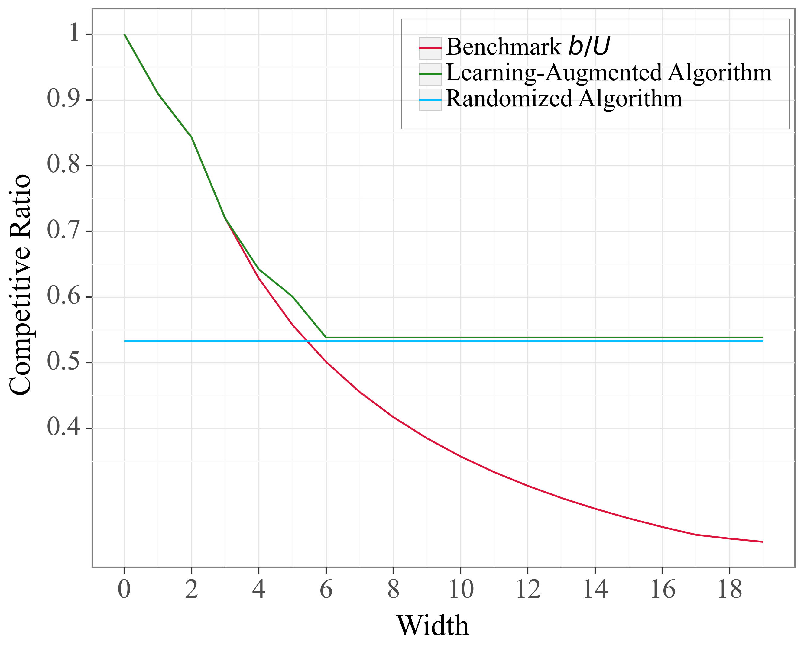
Refer to caption
Refer to caption
Refer to caption
Figure 4: Average competitive ratio under learning-augmented setting. Left: T=22𝑇22T=22, τ=Int[0.2(T+b)]superscript𝜏Intdelimited-[]0.2𝑇𝑏\tau^{*}=\text{Int}[0.2(T+b)]; Middle: T=100𝑇100T=100, τ=Int[0.2(T+b)]superscript𝜏Intdelimited-[]0.2𝑇𝑏\tau^{*}=\text{Int}[0.2(T+b)]; Right: T=100𝑇100T=100, τ=Int[0.1(T+b)]superscript𝜏Intdelimited-[]0.1𝑇𝑏\tau^{*}=\text{Int}[0.1(T+b)].

C.2 Budget Utilization by Each Algorithm

To assess the budget utilization by each algorithm, we eliminate the penalty term from the objective in Problem 2.1. Figures 5 and 6 display the average competitive ratios in scenarios without and with learning augmentation, respectively. We note that in Figure 5 (middle), when τ=22superscript𝜏22\tau^{*}=22, the competitive ratio slightly exceeds 1. This is attributed to our algorithm utilizing a slightly higher budget in expectation. We provide detailed insights into this observation in Appendix A.1, where we demonstrate that the worst-case budget spent is about 1.044bk1.044subscript𝑏𝑘1.044b_{k}, slightly surpassing the allocated budget.
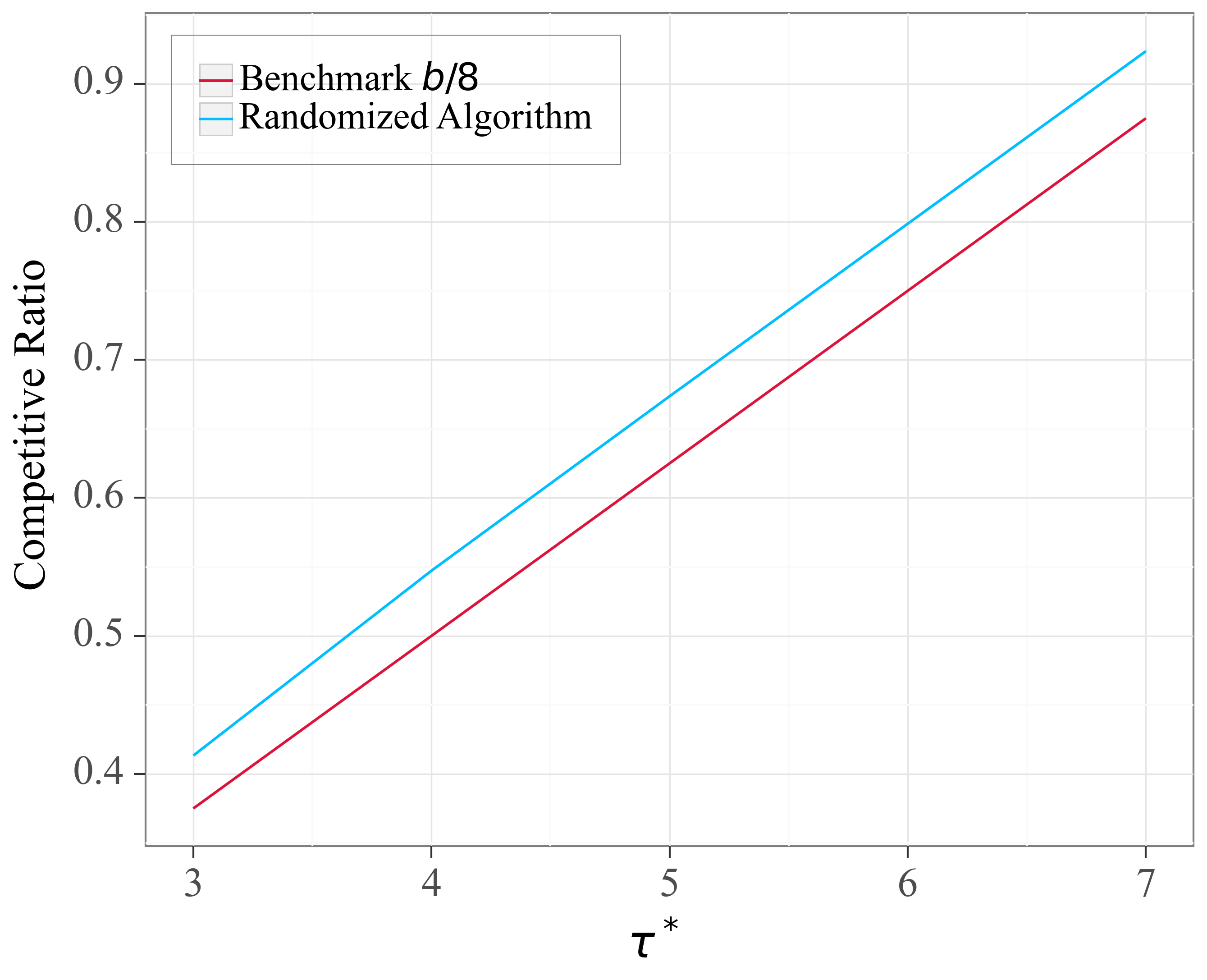
Refer to caption
Refer to caption
Refer to caption
Figure 5: Average competitive ratio under non-learning augmented setting. Left: T=8𝑇8T=8; Middle: T=22𝑇22T=22; Right: T=100𝑇100T=100.
Refer to caption
Refer to caption
Refer to caption
Figure 6: Average competitive ratio under learning-augmented setting. Left: T=8𝑇8T=8, τ=Int[0.5(T+b)]superscript𝜏Intdelimited-[]0.5𝑇𝑏\tau^{*}=\text{Int}[0.5(T+b)]; Middle: T=22𝑇22T=22, τ=Int[0.5(T+b)]superscript𝜏Intdelimited-[]0.5𝑇𝑏\tau^{*}=\text{Int}[0.5(T+b)]; Right: T=100𝑇100T=100, τ=Int[0.5(T+b)]superscript𝜏Intdelimited-[]0.5𝑇𝑏\tau^{*}=\text{Int}[0.5(T+b)].

Appendix D Additional Results on HeartSteps V1 Study

In the HeartSteps V1 application, we implement four algorithms: our randomized and learning-augmented algorithms (Algorithms 1 and 2, respectively), the SeqRTS strategy proposed by Liao et al. (2018), and a benchmark method (b/U𝑏𝑈b/U).

Rather than devising a tailored prediction model, we generate prediction intervals by randomly selecting from a range of [2,144]2144[2,144], which contains τsuperscript𝜏\tau^{*}, with intervals of varying widths. This approach allows us to assess the performance of different algorithms under varying qualities of forecast accuracy.

We adopt the SeqRTS method to include prediction intervals, ensuring a balanced comparison with our algorithms. At the start of each user day, a number is randomly selected from the interval [L,U]𝐿𝑈[L,U] to estimate the number of available risk times. Should the budget be exhausted before allocating for all available risk times, a minimum probability of 1×1061superscript1061\times 10^{-6} is assigned to the remaining times. For additional information on the SeqRTS method, readers are referred to Liao et al. (2018).

Figure 7 illustrates the average entropy change across user days. It is evident that SeqRTS exhibits the highest entropy change, suggesting non-uniform distribution behavior. In contrast, our learning-augmented algorithm demonstrates superior uniformity, outperforming the randomized algorithm. The benchmark method records an entropy of zero, attributed to its conservative strategy of assigning a constant probability of b/U𝑏𝑈b/U.

Figure 8 shows the average competitive ratio and entropy change across user days, considering the scenario where SeqRTS assigns a minimum probability of 00 to remaining risk times once the budget is depleted. Owing to the Penalization term 2, this results in the objective function being negative infinity and the entropy change reaching infinity.
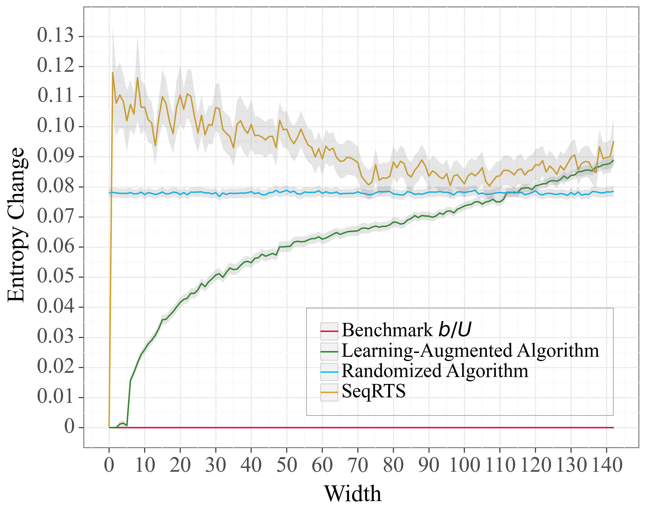
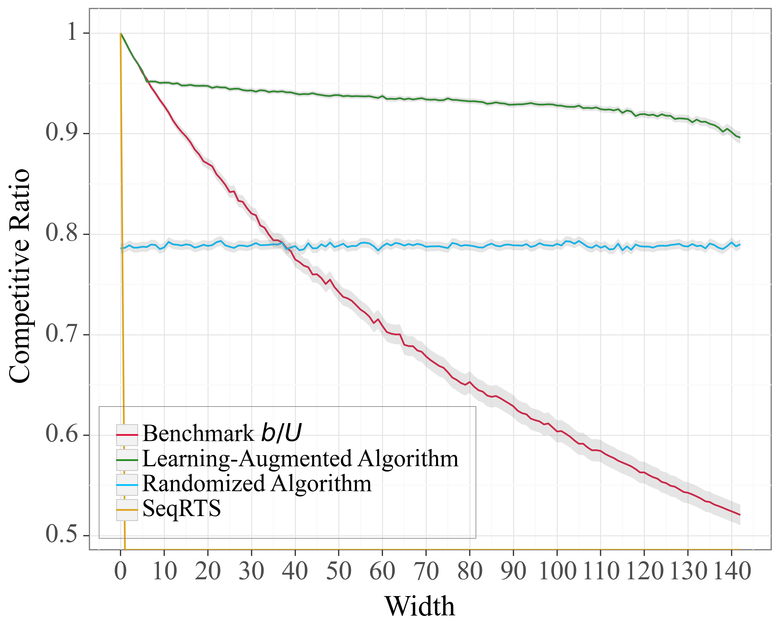
Refer to caption
Figure 7: Entropy change averaged across user days under various prediction interval widths on the HeartSteps V1 dataset. The shaded area represents the ±1.96plus-or-minus1.96\pm 1.96 standard error bounds across user days.
Refer to caption
Refer to caption
Figure 8: Competitive ratio and entropy change averaged across user days under various prediction interval widths on the HeartSteps V1 dataset. The shaded area represents the ±1.96plus-or-minus1.96\pm 1.96 standard error bounds across user days. Note: For SeqRTS, a minimum probability of 00 is assigned to the remaining times when the budget is exhausted.