Combining T-learning and DR-learning:
a framework for oracle-efficient estimation of causal contrasts

Abstract

We introduce efficient plug-in (EP) learning, a novel framework for the estimation of heterogeneous causal contrasts, such as the conditional average treatment effect and conditional relative risk. The EP-learning framework enjoys the same oracle-efficiency as Neyman-orthogonal learning strategies, such as DR-learning and R-learning, while addressing some of their primary drawbacks, including that (i) their practical applicability can be hindered by loss function non-convexity; and (ii) they may suffer from poor performance and instability due to inverse probability weighting and pseudo-outcomes that violate bounds. To avoid these drawbacks, EP-learner constructs an efficient plug-in estimator of the population risk function for the causal contrast, thereby inheriting the stability and robustness properties of plug-in estimation strategies like T-learning. Under reasonable conditions, EP-learners based on empirical risk minimization are oracle-efficient, exhibiting asymptotic equivalence to the minimizer of an oracle-efficient one-step debiased estimator of the population risk function. In simulation experiments, we illustrate that EP-learners of the conditional average treatment effect and conditional relative risk outperform state-of-the-art competitors, including T-learner, R-learner, and DR-learner. Open-source implementations of the proposed methods are available in our R package hte3.

1 Introduction

1.1 Background

In recent years, there has been a surge in interest in the development of tools designed for the flexible estimation of causally interpretable functions through the use of machine learning techniques. Many of these functions constitute subgroup-specific contrasts possibly describing heterogeneous treatment effects. Notable examples of such functions include the conditional average treatment effect (CATE) (Robins, 2004, Kennedy, 2020), conditional relative risk (CRR) (van der Laan et al., 2007, Richardson et al., 2017, Qiu et al., 2019), and causal conditional log-odds ratio (Vansteelandt and Goetghebeur, 2003, Robins and Rotnitzky, 2004, Tchetgen Tchetgen et al., 2010). Under causal conditions, these functions can be expressed in terms of quantities estimable from randomly sampled data; often, these quantities involve outcome regressions, that is, conditional means of the outcome given certain baseline covariates and treatment levels.

Plug-in estimation, also known as T-learning (Künzel et al., 2019), offers a straightforward approach for estimating heterogeneous causal contrasts. In this approach, outcome regressions are estimated and then directly substituted into the contrast to compute the causal quantity of interest. However, a limitation of T-learners is that their performance is heavily dependent on the quality of the outcome regression estimators. This sensitivity is undesirable as the form of the outcome regressions can be significantly more complex — and therefore more difficult to estimate — than that of the causal contrast of interest. For example, the outcome regressions can be highly non-smooth, even if the conditional average treatment effect is constant. Consequently, there is a need for developing estimation methodologies that leverage the parsimony of the contrast function when feasible, while maintaining sufficient flexibility to accommodate complex functional forms (Luedtke and van der Laan, 2016a, Kennedy, 2020, Nie and Wager, 2020).

As a means of estimating a causal contrast, it is natural to first identify a risk function for this particular contrast. When an estimator for such risk function is available, contrasts can be estimated using flexible supervised learning tools such as regularized empirical risk minimizers (Van de Geer, 2000), random forests (Breiman, 2001), and gradient boosting (Freund and Schapire, 1997), among others. However, estimating a risk function can be challenging, particularly when the loss function depends on unknown nuisance functions. For instance, the DR-learner loss (van der Laan, 2013, Luedtke and van der Laan, 2016a, Kennedy, 2020) and R-learner loss (Nie and Wager, 2020, Wager and Athey, 2018) for CATE estimation as well as the E-learner loss (Jiang et al., 2019) for CRR estimation depend on the outcome regression and propensity score. When a nonparametric efficient estimator of the resulting risk is used, the empirical risk minimizer based on estimated nuisance functions often estimates the causal contrast as accurately as the (oracle) empirical risk minimizer using the true nuisance functions (Wager and Athey, 2018, Foster and Syrgkanis, 2019, Kennedy, 2020, van der Laan et al., 2023). In parametric settings, an empirical risk minimizer based on an efficient risk estimator is typically efficient for the causal contrast under certain regularity conditions (van der Vaart, 1991, McClean et al., 2022, van der Laan et al., 2023) — this motivates the use of an efficient risk estimator in such problems. In nonparametric settings, to our knowledge, such a general statement is not currently available. However, the advantages of using an efficient risk estimator have been theoretically established in the case of certain causal functions (Theorem 3 of Kennedy et al., 2015; Theorems 1 and 5 of Athey and Wager, 2021) and validated numerically for estimating the CATE (Kennedy, 2020, van der Laan et al., 2023).

Many efficient estimators of commonly used causal contrast risks are based on loss functions that are Neyman-orthogonal (Robins et al., 1995, van der Laan and Robins, 2003, Chernozhukov et al., 2018, Foster and Syrgkanis, 2019), including those leveraged by DR-learner and R-learner (Foster and Syrgkanis, 2019). In most instances in the literature, a Neyman-orthogonal loss is derived, either explicitly or implicitly, by debiasing an initial plug-in risk estimator using the one-step estimation methodology (Pfanzagl and Wefelmeyer, 1985, Bickel et al., 1993). However, there are two substantial drawbacks associated with efficient risk estimators built upon Neyman-orthogonal loss functions. First, Neyman-orthogonal loss functions can be nonconvex, even when they are derived by orthogonalizing a convex loss function. For instance, the Neyman-orthogonal losses associated with the E-learning risk for the CRR (Jiang et al., 2019, Qiu et al., 2019) and the bound-enforcing risk for the CATE (Luedtke and van der Laan, 2016a) are nonconvex. Specifically, they can be expressed as weighted logistic regression loss functions with weights that may take negative values. This is especially problematic as numerous supervised learning implementations, including widely used software for fitting generalized additive models (Wood, 2011), random forests (Wright and Ziegler, 2017), and gradient-boosted regression trees (Chen and Guestrin, 2016), necessitate nonnegative weights. Second, in certain scenarios, empirical risk minimizers based on Neyman-orthogonal loss functions may yield extreme and unrealistic values for the causal contrast of interest. For example, when the outcome is binary, DR-learners (van der Laan, 2013, Kennedy, 2020) may output treatment effect estimates residing outside of $[-1,1]$, which is undesirable since the true CATE is confined within this interval. This failure to respect known bounds arises because fitting DR-learner involves regressing a pseudo-outcome on the covariates of interest, and this pseudo-outcome can take extreme values since it involves inverse-weighting by the estimated propensity score.

The inherent limitations of efficient risk estimators based on Neyman-orthogonal losses have been recognized in the literature, and several strategies have been proposed to address them. As these efficient risk estimators can yield nonconvex loss functions, researchers may opt for risk estimators derived from convex loss functions, even despite their inefficiency. Common examples include inverse-probability-weighted (Luedtke and van der Laan, 2016b, Jiang et al., 2019) or plug-in (Curth and van der Schaar, 2021) risk estimators, which often fail to achieve parametric-rate consistency when the nuisance functions are estimated flexibly. To circumvent the sensitivity of DR-learners to extreme propensity score estimates, Nie and Wager (2020) introduced the R-learner, which is based on a weighted variant of the DR-learner loss function (Morzywolek et al., 2023). Specifically, the R-learner loss function employs overlap weights to down-weight observations in the tails of the propensity score distribution (Li et al., 2018, Vansteelandt and Dukes, 2020, Morzywolek et al., 2023). As a result, when properly tuned, R-learners, unlike DR-learners, avoid using inverse propensity weighting and are less likely to output predictions that violate bounds. However, the choice of weights by the R-learner prioritizes certain regions of the covariate space over others. This prioritization may not always align with subject-matter considerations.

1.2 Our contributions

In this manuscript, we provide a method for estimating causal contrasts based on a novel efficient plug-in risk estimator. Rather than focusing on a single risk function for a particular contrast, such as the CATE, we study a general class of risk functions that can be used to estimate this well-studied contrast and many others, including the CRR function. As we will show, our proposed estimators overcome the drawbacks of efficient one-step risk estimators described in the previous section. Our main contributions are as follows:

1. we introduce the EP-learner for estimating causal contrasts, which is based on a novel efficient plug-in (EP) risk estimator;

2. we establish that, under reasonable conditions, the EP-learner is oracle-efficient, being asymptotically equivalent to the minimizer of an oracle-efficient one-step risk estimator;

3. we introduce EP-learners for the CATE and CRR functions, both of which are doubly robust.

2 Problem setup

2.1 Data structure and notation

Suppose that we have at our disposal a sample of $n$ independent and identically distributed observations, $O_{1},O_{2},\dots,O_{n}$, of the data structure $O=(W,A,Y)$ drawn from a probability distribution $P_{0}$ belonging to a nonparametric statistical model $\mathcal{M}$. In this data structure, $W\in\mathcal{W}\subset\mathbb{R}^{d}$ is a vector of baseline covariates, $A\in\mathcal{A}\subset\mathbb{R}$ is a possibly continuous treatment assignment, and $Y\in\mathbb{R}$ is a bounded real-valued outcome. These observations may arise from an observational study or a randomized controlled trial. We let $\{Y^{a}:a\in\mathcal{A}\}$ be the set of potential outcomes associated with the observed data structure $(W,A,Y)$ (Rubin, 2005), where $Y^{a}$ is the outcome that would have been observed if, possibly contrary to fact, treatment $a\in\mathcal{A}$ had been administered.

For a given distribution $P\in\mathcal{M}$ and a generic realization $(a,w)$ of $(A,W)$, we denote the outcome regression by $\mu_{P}(a,w):=E_{P}(Y\,|\,A=a,W=w)$ and the propensity score by $\pi_{P}(a\,|\,w):=P(A=a\,|\,W=w)$. Further, we denote $\mu^{a}(w):=\mathbb{E}(Y^{a}\,|\,W=w)$, where $\mathbb{E}$ denotes the expectation under the joint distribution of the covariates $W$ and the potential outcomes. Throughout, we let $E_{0}^{n}$ denote the expectation with respect to the product measure $P_{0}^{n}$ from which $(O_{1},O_{2},\ldots,O_{n})$ is drawn. Further, we denote by $P_{0,W}$ the marginal distribution of $W$ under $P_{0}$, and by $\left\lVert f\right\rVert$ and $\left\lVert f\right\rVert_{\infty}$ the $L^{2}(P_{0})$ and $P_{0}$–essential supremum norm, respectively, of a given function $f\in L^{2}(P_{0})$. For notational convenience, we denote the set $[m]:=\{1,2,\dots,m\}$ for $m\in\mathbb{N}$ and write $\mathcal{S}_{0}$ to denote any summary $\mathcal{S}_{P_{0}}$ of the true distribution $P_{0}$.

2.2 Statistical goal

In this paper, we consider estimation of any causal summary $\theta_{0}=\operatorname*{argmin}_{\theta\in\overline{\mathcal{F}}}R_{0}(\theta)$ that can be identified, under suitable conditions, as the minimizer of a population risk function $R_{0}$ over the $L^{2}(P_{0,W})$–closure $\overline{\mathcal{F}}$ of a (convex) action space $\mathcal{F}$. Here, we restrict our attention to risk functions of the form $R_{0}:=R_{P_{0}}$, where $R_{P}(\theta):=E_{P}[L_{\mu_{P}}(W,\theta)]$ with loss function

$$L_{\mu_{P}}(w,\theta):=h_{1}(\theta(w))\sum_{s\in\mathcal{A}}c_{s,1}g_{1}(\mu_{P}(s,w))+h_{2}(\theta(w))\sum_{s\in\mathcal{A}}c_{s,2}g_{2}(\mu_{P}(s,w))$$ (1)

for arbitrary functions $g_{1},g_{2}:\mathbb{R}\rightarrow\mathbb{R}$ with a Lipschitz derivative, twice-differentiable Lipschitz functions $h_{1},h_{2}:\mathbb{R}\rightarrow\mathbb{R}$ with a continuous second derivative, and known constants $c_{a,1},c_{a,2}$ for $a\in\mathcal{A}$. Notably, any summary of the form $\theta_{0}:w\mapsto\sum_{a\in\mathcal{A}}c_{a}f(\mu_{a}(w))$ with constants $c_{a}\in\mathbb{R}$ and fixed function $f:\mathbb{R}\rightarrow\mathbb{R}$ can be expressed in this manner. The CATE and CRR functions are notable examples of such summaries.

Example 1 (label=ex1, name=conditional average treatment effect).

The CATE $\theta_{0}^{-}:w\mapsto\mu_{0}(1,w)-\mu_{0}(0,w)$ minimizes the risk $\theta\mapsto R_{0}^{-}(\theta)$ over $L^{2}(P_{0,W})$, where we define

$$R_{P}^{-}(\theta):=E_{P}\left[\theta(W)^{2}-2\theta(W)\left\{\mu_{P}(1,W)-\mu_{P}(0,W)\right\}\right].$$ (2)

This risk function is obtained by taking $\mathcal{A}=\{0,1\}$, $h_{1}(\theta)=\theta^{2}$, $h_{2}(\theta)=-2\theta$, $g_{1}\circ\mu=1$, $g_{2}\circ\mu=\mu$, $c_{1,1}=1,\,c_{0,1}=0$, $c_{1,2}=1$ and $c_{0,2}=-1$. We note that this same risk function can be used to learn any $V$-specific CATE function $v\mapsto E_{0}[\mu_{0}(1,W)-\mu_{0}(0,W)\,|\,V=v]$ for a coarsened covariate vector $V:=f(W)$ with $f:\mathcal{W}\rightarrow\mathcal{V}\subseteq\mathbb{R}^{d_{0}}$ and $d_{0}\leq d$. For example, $V$ may represent a subset of components of $W$. This is achieved by minimizing $\theta\mapsto R_{0}^{-}(\theta)$ over $L^{2}(P_{0,V})$, where $P_{0,V}$ denotes the distribution of $f(W)$ under sampling from $P_{0}$, rather than $L^{2}(P_{0,W})$ (Morzywolek et al., 2023).

Example 2 (label=ex2, name=conditional relative risk).

When the outcome $Y$ is binary or nonnegative, the log-CRR function $\theta_{0}^{\div}:w\mapsto\log\mu_{0}(1,w)-\log\mu_{0}(0,w)$ minimizes the risk $\theta\mapsto R_{0}^{\div}(\theta)$ over $L^{2}(P_{0,W})$ (Jiang et al., 2019, Qiu et al., 2019), where we define

$$R_{P}^{\div}(\theta):=E_{P}\left[\left\{\mu_{P}(1,W)+\mu_{P}(0,W)\right\}\log(1+\exp\{\theta(W)\})-\mu_{P}(1,W)\theta(W)\right].$$ (3)

This risk function is obtained by taking $\mathcal{A}=\{0,1\}$, $h_{1}(\theta)=\log(1+\exp(\theta))$, $h_{2}(\theta)=-\theta$, $g_{1}(\mu)=g_{2}(\mu)=\mu$, $c_{0,1}=c_{1,1}=1$, $c_{0,2}=0$ and $c_{1,2}=1$. Similarly as in Example 2, for a coarsened covariate vector $V:=f(W)$, this risk function can also be used to learn the $V$-specific CRR function $v\mapsto\log E_{0}[\mu_{0}(1,W)\,|\,V=v]-\log E_{0}[\mu_{0}(0,W)\,|\,V=v]$.

We assume that the loss function giving rise to $R_{0}$ is $\gamma$–strongly convex (Equation 14.42 of Wainwright, 2019) — in Lemma 15, we show that this condition suffices for the existence and uniqueness of $\theta_{0}$. In Lemma 16, we show that this strong convexity holds whenever there exists a constant $\gamma>0$ such that $\sum_{a\in\mathcal{A}}c_{a,1}g_{1}(\mu_{0}(a,W))\not=0$, $\ddot{h}_{2}(\theta(W))\not=0$ and

$$\frac{\ddot{h}_{1}(\theta(W))}{\ddot{h}_{2}(\theta(W))}>-\frac{\sum_{a\in\mathcal{A}}c_{a,2}g_{2}(\mu_{0}(a,W))}{\sum_{a\in\mathcal{A}}c_{a,1}g_{1}(\mu_{0}(a,W))}+\frac{\gamma}{\ddot{h}_{2}(\theta(W))\sum_{a\in\mathcal{A}}c_{a,1}g_{1}(\mu_{0}(a,W))}$$

both hold $P_{0}$–almost surely. Here, for $m\in\{1,2\}$, we denote the first derivatives of $g_{m}$ and $h_{m}$ as $\dot{g}_{m}$ and $\dot{h}_{m}$, respectively, and the second derivative of $h_{m}$ by $\ddot{h}_{m}$. These conditions apply to both the CATE and CRR examples introduced above — see Examples 14.16 and 14.18 in Wainwright (2019) for details.

2.3 Our proposed approach: EP-learning

Given a population risk function $R_{0}$, it is natural to estimate the causal summary $\theta_{0}$ using empirical risk minimization techniques based on an efficient estimator of $R_{0}$. In the existing literature, an ‘orthogonal learning’ strategy is often employed, wherein an efficient risk estimator is derived from a Neyman-orthogonal loss function (Foster and Syrgkanis, 2019). Such a strategy benefits from relative insensitivity to the accuracy of involved nuisance estimators. In this section, we introduce, at a high level, our proposed EP-learning framework — an alternative approach to orthogonal learning — based on a novel, efficient plug-in estimator for the class of population risk functions under consideration.

To derive an efficient estimator of $R_{0}$, in the context of either orthogonal or EP-learning, we exploit the fact that the population risk parameter $P\mapsto R_{P}(\theta)$ at a specified $\theta\in\overline{\mathcal{F}}$ is a pathwise differentiable parameter under $\mathcal{M}$ and therefore amenable to nonparametric efficient estimation using standard techniques. Pathwise differentiability implies the existence of a nonparametric efficient influence function of the $\theta$–specific population risk parameter, the variance of which provides the generalized Cramér-Rao lower bound for estimating $R_{0}(\theta)$. Specifically, under regularity conditions, for given $\theta\in\overline{\mathcal{F}}$, this efficient influence function has the form

$$D_{P,\theta}:(w,a,y)\mapsto L_{\mu_{P}}(\theta,w)+\Delta_{\pi_{P},\mu_{P}}(w,a,y;\theta)-R_{P}(\theta)\ ,$$

where, letting $H_{m,\mu_{P}}(a,w):=c_{a,m}\cdot\dot{g}_{m}(\mu_{P}(a,w))$ for $m\in\{1,2\}$, we write

$$\Delta_{\pi_{P},\mu_{P}}(w,a,y;\theta):=\frac{1}{\pi_{P}(a,w)}\left\{\sum_{m\in\{1,2\}}H_{m,\mu_{P}}(a,w)h_{m}(\theta(w))\right\}\left\{y-\mu_{P}(a,w)\right\}.$$

In the theorem below, we formalize this fact. To do so, we require the following overlap condition:

1. $P(\pi_{P}(a\,|\,W)>\delta)=1$ for all $a\in\mathcal{A}$ and $P\in\mathcal{M}$.

Theorem 1.

Suppose Condition A1 holds. Then, for an arbitrary element $\theta\in\overline{\mathcal{F}}$, the nonparametric efficient influence function of $P^{\prime}\mapsto R_{P^{\prime}}(\theta)$ at $P\in\mathcal{M}$ is given by $D_{P,\theta}$.

Knowledge of this efficient influence function is important because it encodes, in first order, the sensitivity of the population risk to perturbations in its nuisance parameters and facilitates the debiasing of plug-in estimators. We note that $D_{P,\theta}$ can be composed into a sum of three terms: the plug-in loss function $L_{\mu_{P}}$, a weighted residual $\Delta_{\pi_{P},\mu_{P}}$ of the outcome regression $\mu_{P}$, and the negative population risk $-R_{P}(\theta)$. Using that $E_{P}[D_{P,\theta}(O)]=0$, this decomposition allows us to deduce that $L_{\mu_{P}}+\Delta_{\pi_{P},\mu_{P}}$ is a Neyman-orthogonal loss function for $R_{P}$.

Let $\pi_{n}$ and $\mu_{n}$ be estimators of $\pi_{0}$ and $\mu_{0}$, respectively, which we assume for the time being are obtained using an independent dataset; later, we will describe approaches to use cross-fitting when such an independent dataset is not available. Given these nuisance estimators, a one-step debiased estimator of the $\theta$–specific risk $R_{0}(\theta)$ is given by

$$R_{n,\pi_{n},\mu_{n}}(\theta):=\frac{1}{n}\sum_{i=1}^{n}L_{\mu_{n}}(\theta,W_{i})+\frac{1}{n}\sum_{i=1}^{n}\Delta_{\pi_{n},\mu_{n}}(O_{i};\theta)\ .$$ (4)

This estimator can be seen as a debiased version of the plug-in estimator $\frac{1}{n}\sum_{i=1}^{n}L_{\mu_{n}}(\theta,W_{i})$ with debiasing term $\frac{1}{n}\sum_{i=1}^{n}\Delta_{\pi_{n},\mu_{n}}(O_{i};\theta)$. Under appropriate conditions, $R_{n,\pi_{n},\mu_{n}}(\theta)$ is an asymptotically efficient estimator of $R_{0}(\theta)$.

The decomposition in (4) suggests two approaches for learning $\theta_{0}$ based on an efficient estimator of $R_{0}$. One approach, orthogonal learning, uses loss-based learning techniques based on the orthogonalized loss $L_{\mu_{n}}+\Delta_{\pi_{n},\mu_{n}}$, that is, it relies on using the debiased risk estimator $R_{n,\pi_{n},\mu_{n}}$. The alternative approach we propose, EP-learning, instead relies on the risk estimator $R^{*}_{n}:\theta\mapsto\frac{1}{n}\sum_{i=1}^{n}L_{\mu_{n}^{*}}(\theta,W_{i})$, where $\mu_{n}^{*}$ is a carefully constructed estimator of $\mu_{0}$ that negates the need for the debiasing term $\frac{1}{n}\sum_{i=1}^{n}\Delta_{\pi_{n},\mu_{n}^{*}}(O_{i};\theta)$. In this sense, EP-learning follows the spirit of targeted minimum loss-based estimation (TMLE) (van der Laan and Rose, 2011, Luedtke et al., 2017).

The EP-learner algorithm is designed to attain, on one hand, the oracle-efficiency of orthogonal learning strategies based on the loss $L_{\mu_{n}}+\Delta_{\pi_{n},\mu_{n}}$, and on the other hand, the desirable properties — stability and loss convexity — enjoyed by plug-in estimation strategies based on the ‘naive’ loss $L_{\mu_{n}}$. Rather than substituting any ‘good’ estimator of $\pi_{0}$ and $\mu_{0}$ into the orthogonal loss function, in EP-learning, an outcome regression estimator $\mu_{n}^{*}$ is constructed from $\mu_{n}$ through a sieve-based adjustment to ensure that the debiasing term $\frac{1}{n}\sum_{i=1}^{n}\Delta_{\pi_{n},\mu_{n}^{*}}(O_{i};\theta)$ is negligible across values of $\theta$, rendering explicit debiasing unnecessary. Since the difference between $R_{n}^{*}$ and $R_{\pi_{n},\mu_{n}^{*}}$ is negligible, the EP-learner risk estimator benefits both from the plug-in property of the loss $L_{\mu_{n}^{*}}$ and the orthogonality property of the orthogonalized loss $L_{\mu_{n}^{*}}+\Delta_{\pi_{n},\mu_{n}^{*}}$. The precise procedure for building the estimator $\mu_{n}^{*}$ is detailed later in Algorithm 1 and our EP-learner of $\theta_{0}$ is presented in Section 4. In the next section, we illustrate how the plug-in property of EP-learning resolves the issues with Neyman-orthogonal learning referred to in the Introduction.

The concurrent work of Vansteelandt and Morzywołek (2023) similarly uses sieves to construct a debiased plug-in risk estimator, although they restrict their attention to estimation of a covariate-adjusted conditional mean. Their risk is a special case of (1) with $\mathcal{A}=\{1\}$, $h_{1}(\theta)=\theta^{2}$, $h_{2}(\theta)=-2\theta$, $g_{1}\circ\mu=1$, $g_{2}\circ\mu=\mu$, $c_{1,1}=1$, and $c_{0,1}=0$. Besides considering a general class of risks, our approach uses a different form of cross-fitting and sieve-based adjustment to ensure the asymptotic equivalence of our EP-learner risk estimator with an oracle-efficient one-step risk estimator. This difference complicates our theoretical analysis, as it prohibits us from invoking statistical learning bounds based on sample-split nuisance estimators (Foster and Syrgkanis, 2019).

3 Limitations of existing Neyman-orthogonal learning strategies

3.1 Sensitivity of CATE DR-learner to large propensity weights

For estimation of the CATE, the DR-learner is a popular orthogonal learning approach based on the least-squares empirical risk function

$$\theta\mapsto\frac{1}{n}\sum_{i=1}^{n}\left\{\theta(W_{i})^{2}-2\theta(W_{i})\chi_{n}(W_{i},A_{i},Y_{i})\right\},$$

where $\chi_{n}(w,a,y):=\mu_{n}(1,w)-\mu_{n}(0,w)+\frac{2a-1}{\pi_{n}(a\,|\,w)}\left[y-\mu_{n}(a,w)\right]$ is an estimated pseudo-outcome. Notably, this empirical risk is equal to the debiased risk estimator $R_{n,\pi_{n},\mu_{n}}$ of the population risk $R_{0}^{-}$ introduced in Example 2. As discussed in the Introduction, the pseudo-outcome used by DR-learner can take extreme values when the propensity of treatment takes values close to zero or one, which can in turn result in poor behavior of an estimator of the CATE.

In contrast to DR-learner, our EP-learner — formally defined in Section 4 — is instead based on the estimated pseudo-outcome $\mu_{n}^{*}(1,W)-\mu_{n}^{*}(0,W)$, where $\mu_{n}^{*}$ is an estimate of the outcome regression carefully derived from initial estimates $\mu_{n}$ and $\pi_{n}$. Unlike a typical T-learner, this estimate is constructed to ensure that the resulting plug-in risk estimator

$$R_{n}^{*-}(\theta):=\frac{1}{n}\sum_{i=1}^{n}\left[\theta(W_{i})^{2}-2\theta(W_{i})\left\{\mu_{n}^{*}(1,W_{i})-\mu_{n}^{*}(0,W_{i})\right\}\right]$$

is efficient under reasonable conditions. The construction of $\mu_{n}^{*}$ incorporates an inverse-propensity-weighted second-stage regression adjustment of $\mu_{n}$ that renders the corresponding risk estimator doubly robust, in the sense that, for each $\theta$, $R_{n}^{*-}(\theta)$ is consistent if either the outcome regression or propensity score is estimated consistently.

We now provide a heuristic explanation of why EP-learner can outperform DR-learner, particularly when paired with a local regression estimator, such as a Nadaraya-Watson (Nadaraya, 1964, Watson, 1964), $K$-nearest neighbors (Fix and Hodges, 1989), or random forest (Breiman et al., 1984) estimator. When used in a DR-learner or EP-learner, local methods estimate a regression function at a point by averaging the pseudo-outcomes of ‘nearby’ observations. When the number of points averaged is small, the estimates returned by DR-learner can be erratic due to the potentially large values taken by its estimated pseudo-outcomes. In contrast, the EP-learner is expected to be more stable since it is simply a local average of an initial CATE estimator. In fact, if this initial estimator is uniformly consistent, then the corresponding EP-learner remains consistent even when the number of local observations averaged is held fixed with sample size — a formal argument in the case of $K$-nearest neighbors estimation is provided in Appendix D. Moreover, even if the initial estimator fails to be uniformly consistent, then EP-learner can still benefit from the desirable properties that it shares with DR-learner, namely the efficiency and double robustness of its risk estimator — details are provided in Section 5.1.

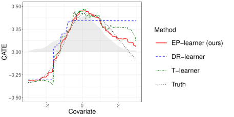
The benefits of EP-learner over DR-learner can be illustrated through a simple numerical experiment. To do so, we simulated a dataset consisting of 1,500 observations and used the ranger implementation of random forests (Wright and Ziegler, 2017) to estimate the CATE function based on both the DR-learner and EP-learner risks — the code used to run our experiment is provided in Appendix B.1. In our illustration, the outcome is binary, and we use the known CATE range, $[-1,1]$, to truncate DR-learner predictions. Figure 1(a) displays the estimated CATE curve for DR-learner and EP-learner with maximum tree depth in random forests selected within $\{1,2,\ldots,7\}$ via 10-fold cross-validation. This figure reveals that the CATE curve estimated using EP-learner more accurately reflects the bell shape of the true CATE curve than using the DR-learner. This improvement is evident quantitatively, with a six-fold reduction in mean squared prediction error when using EP-learner (0.002) compared to DR-learner (0.012). To delve deeper into this phenomenon, we assessed the fits obtained by using four of the seven maximum tree depth values considered, namely 1, 2, 4 and 7 (Figure 1(b)). DR-learner fits become unstable at depths as low as 2, stemming from the limited observation numbers in the regression tree nodes and some pseudo-outcomes reaching magnitudes of 6 — this can be seen in Figure 5 of Appendix B.1. As a result, cross-validation chooses a depth of 1 for DR-learner, which fails to accurately capture the true CATE shape. In contrast, EP-learner fits tend to improve as the maximum depth increases from 1 to 7, with a selected maximum tree depth of 7.

(a) Cross-validated maximum tree depth

(b) Fixed maximum tree depth

Figure 1: CATE estimates based on EP-learner, DR-learner, and T-learner with random forests and various maximum tree depths computed on a single dataset. (Top) EP-learner, DR-Learner, and T-learner CATE estimates with 10-fold cross-validated maximum tree depth; mean squared prediction errors are 0.0021, 0.012, and 0.005, respectively. Observed covariate distribution is depicted in gray. (Bottom) EP-learner, DR-learner,and T-learner CATE estimate for maximum tree depths of 1, 2, 4 and 7.

3.2 Nonconvexity of Neyman-orthogonal CRR loss function

We introduced in Example 2 the population risk function $R_{0}^{\div}$ for the CRR $\theta_{0}^{\div}:w\mapsto\log\mu_{0}(1,w)-\log\mu_{0}(0,w)$. In light of (4), a doubly-robust and efficient one-step debiased risk estimator for the population risk function is given by

$$R_{n,DR}^{\div}(\theta):=\frac{1}{n}\sum_{i=1}^{n}\left[\left(\widehat{\mu}_{0,i}+\widehat{\mu}_{1,i}\right)\log\left(1+\exp\{\theta(W_{i})\}\right)-\widehat{\mu}_{1,i}\theta(W_{i})\right],$$ (5)

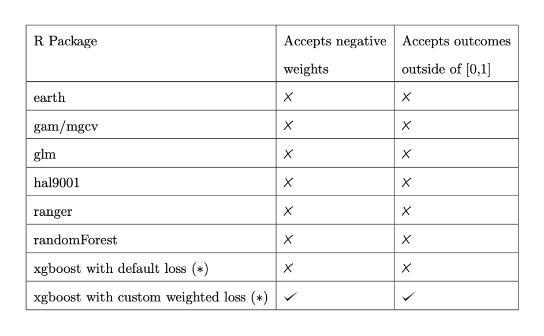
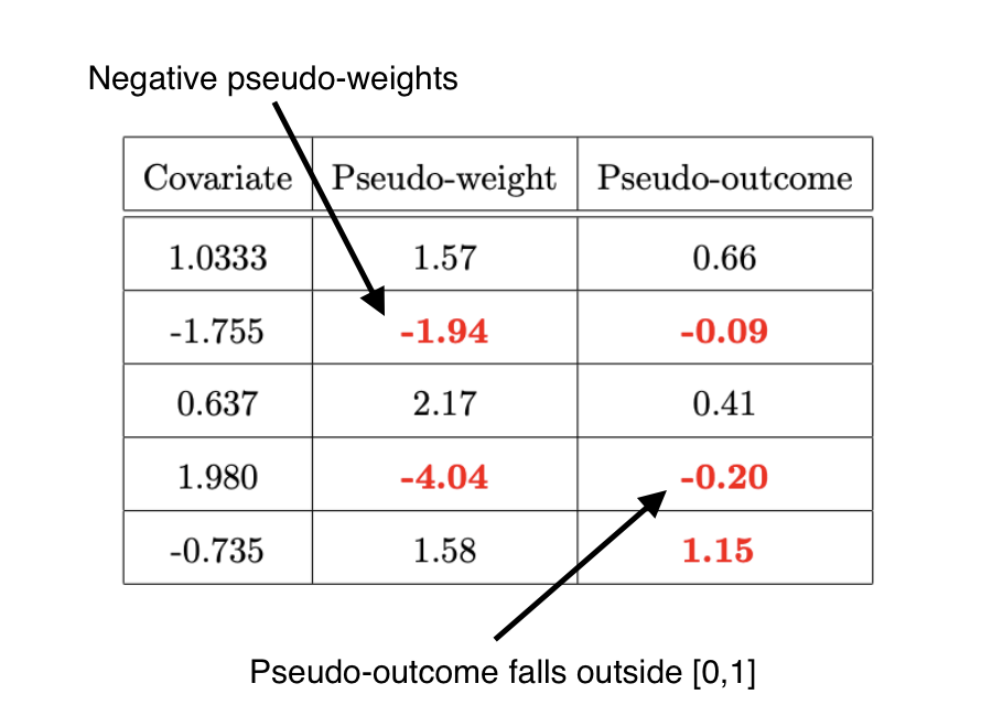
where, for $s\in\{0,1\}$ and $i\in[n]$, we define $\widehat{\mu}_{s,i}:=\mu_{n}(s,W_{i})+\frac{1(A_{i}=s)}{\pi_{n}(s\,|\,W_{i})}\left\{Y_{i}-\mu_{n}(s,W_{i})\right\}$. The corresponding doubly-robust orthogonal learner of the log-CRR function is computed by performing a weighted logistic regression of the pseudo-outcomes $\left\{\widehat{\mu}_{1,i}/(\widehat{\mu}_{0,i}+\widehat{\mu}_{1,i}):i\in[n]\right\}$ on the covariate values $\{W_{i}:i\in[n]\}$ with weights $\left\{\widehat{\mu}_{0,i}+\widehat{\mu}_{1,i}:i\in[n]\right\}$. Because the weights may take negative values, the Neyman-orthogonal loss function associated with the one-step debiased risk estimator may be nonconvex. Furthermore, the pseudo-outcomes may take values outside of $[0,1]$, which renders this a nonstandard use case for logistic regression. Figure 2 lists several common logistic regression implementations in R and indicates whether they allow the use of negative weights or outcomes that fall outside of $[0,1]$. As is revealed in this figure, most do not, which demonstrates the limited applicability of orthogonal learning in this setting. Figure 2 shows the first five rows of a synthetic input dataset containing the covariate values, pseudo-weights and pseudo-outcomes that would be entered into logistic regression software to estimate the log conditional relative risk. Notably, the mock dataset contains negative pseudo-weight values and pseudo-outcomes that fall outside of $[0,1]$. Code to reproduce this dataset can be found in Appendix B.1.

Figure 2: (Left) Common R packages for logistic regression may or may not allow negative weights and outcomes outside of [0,1]; a checkmark indicates that they do. ($\ast$) The xgboost package has many built-in loss functions, but they do not accept negative weights. However, these negative weights can be absorbed into a custom loss function. (Right) Example dataset for estimating the CRR using the one-step efficient risk estimator.

For a post-hoc constructed outcome regression estimator $\mu_{n}^{*}$, our EP-learner of the CRR is based on the following EP risk estimator

$$R_{n,EP}^{\div}(\theta):=\frac{1}{n}\sum_{i=1}^{n}\left\{\mu_{n}^{*}(1,W_{i})+\mu_{n}^{*}(0,W_{i})\right\}\left[\log(1+\exp\{\theta(W_{i})\})-\frac{\mu_{n}^{*}(1,W_{i})}{\mu_{n}^{*}(1,W_{i})+\mu_{n}^{*}(0,W_{i})}\theta(W_{i})\right].$$

An estimator of the log-CRR function based on the EP-learner risk estimator is computed by performing the weighted logistic regression of the pseudo-outcome $\mu_{n}^{*}(1,W)/[\mu_{n}^{*}(1,W)+\mu_{n}^{*}(0,W)]$ onto the covariate vector $W$ with weight $\mu_{n}^{*}(1,W)+\mu_{n}^{*}(0,W)$. Unlike for the efficient one-step risk estimator, the pseudo-weight is always nonnegative and the pseudo-outcome always falls in $[0,1]$. As a consequence, the EP-learner risk estimator corresponds with a convex loss function, and EP-learners of the log-CRR function can be implemented using most standard logistic regression software. In Section 4, we will provide an algorithm to construct $\mu_{n}^{*}$ so that $R_{n,EP}^{\div}$ is an efficient, doubly robust plug-in risk estimator.

4 Proposed approach: EP-learning algorithm

The EP-learner algorithm is designed to attain both the efficiency of the one-step debiased risk estimator in (4) and the desirable properties, such as stability and convexity, that are enjoyed by plug-in risk estimators. This learner is based on a risk function of the form $\theta\mapsto\frac{1}{n}\sum_{i=1}^{n}L_{\mu_{n}}(\theta,W_{i})$ for an outcome regression estimator $\mu_{n}$. Naturally, the fact that EP-learner does not explicitly appear to debias this plug-in estimator may lead to concerns that it might be based on a suboptimal — in particular, inefficient — estimator of the risk. However, the EP-learner outcome regression estimator is carefully constructed to perform implicit debiasing. Specifically, it is designed such that the seemingly-critical debiasing term $\frac{1}{n}\sum_{i=1}^{n}\Delta_{\pi_{n},\mu_{n}}(O_{i};\theta)$ is negligible in an appropriate sense across values of $\theta$, so that the plug-in risk estimator is asymptotically equivalent to a one-step debiased estimator. Before describing the general EP-learner approach, we illustrate its construction in the context of a simple, finite-dimensional example.

Example 3 (continues = ex1, , name=conditional average treatment effect).

Consider the problem of CATE estimation from Example 2 in the special case where the action space $\mathcal{F}$ is the linear class including each function $w\mapsto\alpha^{\top}w$ with $\alpha\in\mathbb{R}^{d}$. In this finite-dimensional case, we write $R_{0}^{-}(\alpha)$ as shorthand for $R_{0}^{-}(w\mapsto\alpha^{\top}w)$. Given initial estimators $\pi_{n}$ of $\pi_{0}$ and $\mu_{n}$ of $\mu_{0}$, EP-learner uses the refined estimator $\mu_{n}^{*}:(a,w)\mapsto\mu_{n}(a,w)+(2a-1)\beta_{n}^{\top}w$, where

$$\beta_{n}:=\operatorname*{argmin}_{\beta\in\mathbb{R}^{d}}\frac{1}{n}\sum_{i=1}^{n}\frac{1}{\pi_{n}(A_{i}\,|\,W_{i})}\left\{Y_{i}-\mu_{n}(A_{i},W_{i})-(2A_{i}-1)\beta^{\top}W_{i}\right\}^{2}.$$

The first-order conditions satisfied by $\beta_{n}$ ensure that the debiasing term for estimating $R_{0}^{-}(\alpha)$, notably $\frac{1}{n}\sum_{i=1}^{n}\frac{2A_{i}-1}{\pi_{n}(A_{i}\,|\,W_{i})}\alpha^{\top}W_{i}\left\{Y_{i}-\mu_{n}^{*}(A_{i},W_{i})\right\}$, is exactly zero for $\alpha\in\mathbb{R}^{d}$. In this special case, the refined outcome regression estimator used by EP-learner corresponds to a targeted minimum loss-based estimator (van der Laan and Rose, 2011) for the gradient of the risk function $\alpha\mapsto R_{0}^{-}(\alpha)$.

When the dimension of the action space $\mathcal{F}$ is large relative to sample size (e.g., infinite action space), it is generally not possible to construct an outcome regression estimator $\mu_{n}$ that both has good predictive performance and makes the debiasing term $\frac{1}{n}\sum_{i=1}^{n}\Delta_{\pi_{n},\mu_{n}}(O_{i};\theta)$ exactly zero for each $\theta\in\mathcal{F}$. Indeed, there is an inherent trade-off between the size of the debiasing term and the mean squared error of the outcome regression estimator. The EP-learner algorithm is designed to carefully balance these two terms. It does so by separating the estimation of the outcome regression into two stages. In the first stage, statistical learning tools are used to obtain an initial estimate of the outcome regression with good predictive performance. In the second stage, this initial estimator is refined to make the debiasing term as small as possible without harming the performance of EP-learner.

The debiasing approach described in Example 3 can be generalized to infinite-dimensional function spaces using the idea of sieves. Specifically, if the linear span of a finite but growing set of basis functions approximates $\mathcal{F}$ increasingly well, then the refinement procedure described in Example 3 could be performed within this span. This procedure would ensure that the debiasing term is small for each element in the linear space spanned by these basis functions. Critically, the number of basis functions used would need to grow with sample size so that the worst-case approximation error tends to zero. Akin to competing procedures such as the DR-Learner and R-learner, EP-learner can incorporate cross-fitting of the initial outcome regression and propensity score estimators for enhanced performance. Below, we detail a general cross-fitted implementation of EP-learner.

Let $J\in\mathbb{N}$ denote a fixed number of cross-fitting splits. Let $\mathcal{D}_{n}^{1},\mathcal{D}_{n}^{2},\ldots,\mathcal{D}_{n}^{J}$ be a partition of the available data $\mathcal{D}_{n}$ into $J$ datasets of approximately equal size, corresponding to index sets $\mathcal{I}^{1}_{n},\mathcal{I}^{2}_{n},\ldots,\mathcal{I}^{J}_{n}$. For each $i\in[n]$, let $j(i)\in[J]$ be the index of the data fold containing observation $i$, so that $i\in\mathcal{I}_{n}^{j(i)}$. Suppose that, for each $j\in[J]$, we have constructed estimators $\pi_{n,j}$ of $\pi_{0}$ and $\mu_{n,j}$ of $\mu_{0}$ based on $\mathcal{D}_{n}\backslash\mathcal{D}_{n}^{j}$. Let $\varphi_{k}:\mathbb{R}^{d}\mapsto\mathbb{R}^{k}$ be a feature mapping such that elements of the transformed action space ${\mathcal{H}}:=\{h_{j}\circ\theta:\theta\in\mathcal{F},j=1,2\}$ are approximated well by the linear space $\mathcal{H}_{k}:=\{w\mapsto\beta^{\top}\varphi_{k}(w):\beta\in\mathbb{R}^{k}\}$, where $k=k(n)$ is typically chosen to grow with $n$. Algorithm 1 transforms, for each $j$, the initial outcome regression estimator $\mu_{n,j}$ into a refined estimator $\mu_{n,j}^{*}$ such that

$$\frac{1}{n}\sum_{i=1}^{n}\frac{1}{\pi_{n,j(i)}(A_{i}\,|\,W_{i})}\left\{\sum_{m\in\{1,2\}}H_{m,\mu_{n,j(i)}}(A_{i},W_{i})\psi_{m}(W_{i})\right\}\left\{Y_{i}-\mu_{n,j(i)}^{*}(A_{i},W_{i})\right\}=0$$ (6)

for each $\psi_{1},\psi_{2}\in\mathcal{H}_{k(n)}$, where $H_{m,n,j}$ is defined as $(a,w)\mapsto c_{a,m}\dot{g}_{m}(\mu_{n,j}(a,w))$ with $c_{a,m}$ and $g_{m}$ introduced in (1). Modifications of this algorithm are possible. For certain population risk functions, including the CATE risk function used in Example 2, Algorithm 1 can be simplified by performing the adjustment over a lower-dimensional space; details are provided in Appendix C.1. It is also possible to implement an alternative debiasing step that preserves bounds on the initial outcome regression estimator, even in cases in which the outcome itself may be unbounded; details are provided in Appendix C.2. Such modification may improve performance by ensuring that the refinement step does not exceed bounds possibly specified a priori and enforced in the initial learning step.

Algorithm 1 Debiasing procedures.

0:  

  – dataset $\mathcal{D}_{n}$ consisting of observations $(W_{1},A_{1},Y_{1}),(W_{2},A_{2},Y_{2}),\ldots,(W_{n},A_{n},Y_{n})$;

  – cross-fitted estimates $\pi_{n,1},\pi_{n,2},\ldots,\pi_{n,J}$ of $\pi_{0}$ and $\mu_{n,1},\mu_{n,2},\ldots,\mu_{n,J}$ of $\mu_{0}$;

  – feature mapping $\varphi_{k}:\mathbb{R}^{d}\mapsto\mathbb{R}^{k}$ of output dimension $k\in\mathbb{N}$;

1:  for each $i\in[n]$, construct $\widehat{\varphi}_{k,j(i)}:\mathbb{R}^{d+1}\mapsto\mathbb{R}^{2k}$ as $(a,w)\mapsto(H_{1,n,i}(a,w),H_{2,n,i}(a,w))\varphi_{k}(w)$ with $H_{1,n,i}(a,w):=c_{a,1}\dot{g}_{1}(\mu_{n,j(i)}(a,w))$ and $H_{2,n,i}(a,w):=c_{a,2}\dot{g}_{2}(\mu_{n,j(i)}(a,w))$;

2:  choose link function $g$ and obtain regression coefficient estimate $\beta_{n}$ as follows:

• method 1: outcomes in $[0,1]$. set $g:x\mapsto\text{logit}(x)$ and $\bar{g}:x\mapsto\text{expit}(x)$, and compute coefficient vector estimate $\beta_{n}$ obtained from logistic regression of outcome $Y_{i}$ on feature vector $\widehat{\varphi}_{k,j(i)}(A_{i},W_{i})$ with offset $\text{logit}\,\mu_{n,j(i)}(A_{i},W_{i})$ and weight $1/\pi_{n,j(i)}(A_{i}\,|\,W_{i})$ for $i\in[n]$;

• method 2: general outcomes. set $g:x\mapsto x$ and $\bar{g}:x\mapsto 1/x$, and compute coefficient vector estimate $\beta_{n}$ obtained from linear regression of outcome $Y_{i}$, on feature vector $\widehat{\varphi}_{k,j(i)}(A_{i},W_{i})$ with offset $\mu_{n,j(i)}(A_{i},W_{i})$ and weight $1/\pi_{n,j(i)}(A_{i}\,|\,W_{i})$ for $i\in[n]$;

3:  for each $j\in[J]$, return debiased out-of-fold outcome regression estimator

$$\mu_{n,j}^{*}:(a,w)\mapsto\bar{g}\left(g(\mu_{n,j}(a,w))+\widehat{\varphi}_{k,j}(a,w)^{\top}\beta_{n}\right).$$ (7)

The EP-learner presented in Algorithm 2 is based on a feature mapping of fixed dimension $k$. Line 2 of this algorithm encompasses many estimation strategies, including penalized empirical risk minimization (Van de Geer, 2000), random forests (Breiman, 2001), and gradient boosting (Freund and Schapire, 1997). Algorithm 3 instead describes a cross-validated EP-learner implementation incorporating data-driven selection of the feature mapping dimension. This selection is made based on a one-step debiased estimate of the risk function. The potential nonconvexity of this risk does not cause computational issues in this case since optimization is performed over a finite set of candidate values of $k$.

Algorithm 2 EP-learner algorithm (fixed sieve dimension)

0:  

  – dataset $\mathcal{D}_{n}$ consisting of observations $(W_{1},A_{1},Y_{1}),(W_{2},A_{2},Y_{2}),\ldots,(W_{n},A_{n},Y_{n})$;

  – cross-fitted estimates $\pi_{n,1},\pi_{n,2},\ldots,\pi_{n,J}$ of $\pi_{0}$ and $\mu_{n,1},\mu_{n,2},\ldots,\mu_{n,J}$ of $\mu_{0}$;

  – feature mapping $\varphi_{k}:\mathbb{R}^{d}\mapsto\mathbb{R}^{k}$ of output dimension $k\in\mathbb{N}$;

  – supervised learning algorithm for causal contrast;

1:  obtain debiased outcome regression estimates $\mu_{n,j}^{*}$ from $\pi_{n,j}$ and $\mu_{n,j}$ using Algorithm 1;

2:  return minimizer $\theta_{n,k}^{*}$ of $\theta\mapsto\frac{1}{n}\sum_{i=1}^{n}L_{\mu^{*}_{n,j(i)}}(\theta,W_{i})$.

Algorithm 3 EP-learner algorithm (cross-validated sieve dimension)

0:  

  – dataset $\mathcal{D}_{n}$ consisting of observations $(W_{1},A_{1},Y_{1}),(W_{2},A_{2},Y_{2}),\ldots,(W_{n},A_{n},Y_{n})$;

  – number of cross-fitting splits $J$;

  – growing sequence $\varphi_{1},\varphi_{2},\ldots,\varphi_{K(n)}$ of feature mappings, with $\varphi_{k}:\mathbb{R}^{d}\mapsto\mathbb{R}^{k}$ and $K(n)\in\mathbb{N}$;

  – supervised learning algorithm for causal contrast;

1:  partition $\mathcal{D}_{n}$ into $J$ datasets $\mathcal{D}_{n}^{1},\mathcal{D}_{n}^{2},\ldots,\mathcal{D}_{n}^{J}$ of approximately equal size, say with corresponding index sets $\mathcal{I}^{1}_{n},\mathcal{I}^{2}_{n},\ldots,\mathcal{I}^{J}_{n}$;

2:  for $j\in[J]$, construct estimates $\pi_{n,j}$ and $\mu_{n,j}$ of $\pi_{0}$ and $\mu_{0}$ using $\mathcal{D}_{n}\,\backslash\,\mathcal{D}_{n}^{j}$;

3:  for $k=1,2,\dots,K(n)$ do

4:     for $j=1,2,\dots,J$ do

5:        obtain debiased estimates $\mu_{n,j,k}^{*}$ from $\pi_{n,j}$ and $\mu_{n,j}$ using Algorithm 1 with dataset $\mathcal{D}_{n}\backslash\mathcal{D}_{n}^{j}$, cross-fitted estimates $\pi_{n,1},\pi_{n,2},\ldots,\pi_{n,J}$ and $\mu_{n,1},\mu_{n,2},\ldots,\mu_{n,J}$, and feature-mapping $\varphi_{k}$;

6:        obtain minimizer $\theta_{n,j,k}^{*}$ of $\theta\mapsto\sum_{i\in[n]\backslash\mathcal{I}_{n}^{j}}L_{\mu^{*}_{n,j(i)}}(\theta,W_{i})$.

7:     end for

8:  end for

9:  compute optimal dimension $k_{cv}(n):=\operatorname*{argmin}_{k\in\mathbb{N}}\frac{1}{n}\sum_{i=1}^{n}L_{\pi_{n,j(i)},\mu_{n,j(i)}}(O_{i},\theta_{n,j(i),k}^{*})$;

10:  return $\theta_{n,k_{cv}(n)}^{*}$ obtained using Algorithm 2 with dataset $\mathcal{D}_{n}$ and feature mapping $\varphi_{k_{cv}(n)}$.

As presented in Algorithm 3, the cross-validated EP-learner only requires the construction of cross-fitted outcome regression and propensity score estimators once. Nuisance estimators do not need to be recomputed within each training fold. Since the cross-fitted nuisance estimators are constructed using the entire dataset, there is some data leakage across the training folds used for cross-validation. To avoid such data leakage, the nuisance functions could alternatively be re-estimated within each training fold, although this would come at a possibly significant computational cost.

The sieve $\mathcal{H}_{1},\mathcal{H}_{2},\ldots$ used in the EP-learner implementation is an important ingredient that must be specified. In some cases, the transformed action space ${\mathcal{H}}$ suggests a natural choice of sieve. For instance, if ${\mathcal{H}}$ is a reproducing kernel Hilbert space, the linear span of the first $k$ elements of the leading eigenfunctions of the integral kernel operator (Mendelson and Neeman, 2010) is a canonical choice for $\mathcal{H}_{k}$. More generally, sieves based on the trigonometric polynomials (Jackson, 1912), B-splines (Gordon and Riesenfeld, 1974), and wavelets (Antoniadis, 2007) are natural candidates with strong approximation guarantees under smoothness assumptions on the action space. In principle, the cross-validated EP-learner could be modified to select from different basis functions used to define the sieve. For example, Algorithm 2 can be used to construct EP-learners based on different subsets of trigonometric polynomial and B-spline basis functions.

5 Theoretical guarantees

5.1 Efficiency of the EP risk estimator

In this section, we study the EP risk estimator presented in Algorithm 2 with a deterministic feature mapping dimension $k=k(n)$ growing with sample size. Specifically, we establish conditions under which this EP risk estimator is equivalent to an oracle-efficient one-step risk estimator. To do so, we show that the debiasing term for the EP-learner risk estimator has a second-order dependence on the estimation error of the outcome regression estimator and the sieve approximation error of the transformed action space ${\mathcal{H}}$. Thus, if this debiasing term converges to zero rapidly enough, the EP-learner risk estimator is $n^{\frac{1}{2}}$–consistent, asymptotically linear, and nonparametric efficient for the population risk uniformly over the action space $\mathcal{F}$, as we formalize below.

For $\theta\in L^{2}(P_{0,W})$, we denote by $\ \|\theta\|_{\infty}$ the $P_{0}$–essential supremum norm and by ${\Pi_{k}\,}\theta\in\operatorname*{argmin}_{\phi\in\mathcal{H}_{k}}\left\lVert\theta-\phi\right\rVert$ the $L^{2}(P_{0})$–projection of $\theta\in\mathcal{H}$ onto the sieve $\mathcal{H}_{k}$. Below, we make use of the following conditions:

1. there exist constants $\eta\in(0,1)$ and $M\in(0,\infty)$ such that, for all $j\in[J]$, for $P_{0}$–almost every realization $(w,a)$ of $(W,A)$, and with $P_{0}$–probability tending to one:

   1. strong positivity: $\pi_{0}(a\,|\,w)\in[\eta,1-\eta]$ and $\pi_{n,j}(a\,|\,w)\in[\eta,1-\eta]$;

   2. boundedness: $|\mu_{n,j}(a,w)|<M$ and $|\mu_{n,j}^{*}(a,w)|<M$;

2. polynomial nuisance rates: there exist $\gamma>0$ and $\beta>\frac{1}{4\gamma}$ such that, for all $j\in[J]$:

   1. propensity score: $\left\lVert\pi_{n,j}-\pi_{0}\right\rVert=\mathcal{O}_{p}\big{(}n^{-\gamma/(2\gamma+1)}\big{)}$;

   2. outcome regression: $\left\lVert\mu_{n,j}-\mu_{0}\right\rVert=\mathcal{O}_{p}\big{(}n^{-\beta/(2\beta+1)}\big{)}$, and $\beta>\frac{1}{2}$ unless both $g_{1}$ and $g_{2}$ are the identify function;

   3. debiased outcome regression: $\|\mu_{n,j}^{*}-\mu_{0}\|=\mathcal{O}_{p}\big{(}n^{-\beta/(2\beta+1)}+\sqrt{k(n)\log n/n}\big{)}$;

3. sufficiently small sieve approximation error: there exist $\rho>\frac{1}{2}$ and $\nu\geq 0$ such that:

   1. slowly growing Lebesgue constant: $\sup_{\phi\in\mathcal{H},v\in\mathcal{H}_{k(n)}}\frac{\|\Pi_{k(n)}(\phi+v)\|_{\infty}}{\|\phi+v\|_{\infty}}=\mathcal{O}\big{(}\{\log k(n)\}^{\nu}\big{)}$;

   2. polynomial approximation rate: $\sup_{\theta\in\mathcal{H}}\inf_{\phi\in\mathcal{H}_{k(n)}}\left\lVert\theta-\phi\right\rVert_{\infty}=\mathcal{O}\big{(}k(n)^{-\rho}\big{)}$;

   3. large enough exponent: if $\min\{\beta,\gamma\}>\frac{1}{2}$, then $\rho\geq\frac{1}{2\beta+1}$, and otherwise, $\rho\geq\frac{1}{4\min\{\beta,\gamma\}}$.

By controlling the Lebesgue constant (Belloni et al., 2012) in C3a, approximation theory can be used to bound $\sup_{\theta\in\mathcal{H}}\|\theta-\Pi_{k(n)}\theta\|_{\infty}$ by the sup-norm approximation error of C3b up to logarithmic dependence on $k(n)$ (Huang, 2003, Chen and Christensen, 2013, Belloni et al., 2012). Only requiring elements of $\mathcal{H}$ to be continuous, Section 3.2 of Belloni et al. (2012) provides an overview of several sieve choices that satisfy this condition, including those based on trigonometric series, splines, wavelets, and local polynomials. Condition C2c is the convergence rate expected for an empirical risk minimizer over a sieve space of dimension $k(n)$ based on a loss indexed by cross-fitted nuisances (Foster and Syrgkanis, 2019). This condition is satisfied under regularity conditions when each $\mu_{n,j}^{*}$ is obtained using Algorithm 1. Together, conditions C2 and C3 ensure the existence of a sequence of sieve dimensions $k(n)$ such that, for each $j\in[J]$, remainder terms of the order $\|\mu_{n,j}^{*}-\mu_{0}\|\left\lVert\pi_{n,j}-\pi_{0}\right\rVert$ and $\sup_{\phi\in{\mathcal{H}}}\|\phi-\Pi_{k(n)}\phi\|\|\mu_{n,j}^{*}-\mu_{0}\|$ are $\mathchoice{{\scriptstyle\mathcal{O}}}{{\scriptstyle\mathcal{O}}}{{\scriptscriptstyle\mathcal{O}}}{\scalebox{0.7}{$\scriptscriptstyle\mathcal{O}$}}_{p}(n^{-\frac{1}{2}})$. The precise choice of $k(n)$ depends on $\beta$, $\gamma$ and $\rho$, which are typically unknown. However, under mild conditions, using arguments similar to those in van der Laan and Dudoit (2003), it can be shown that the cross-validated EP-learner is equivalent to the infeasible EP-learner that uses an oracle selector of $k(n)$ minimizing the population risk.

Compared to cross-fitted empirical risk estimators (Kennedy, 2020, Foster and Syrgkanis, 2019), the nuisance estimator $\mu_{n,j}^{*}$ depends on the entire dataset, and so, the EP-learner loss function $L_{\mu_{n,j}}^{*}$ is not independent of observations in the $j$th fold. Consequently, to obtain tighter control of empirical process remainders (van de Geer, 2014), we require that the action space $\mathcal{F}$ not be too large with respect to the supremum norm metric. To quantify the complexity of $\mathcal{F}$, we consider the $\varepsilon$–covering number $N_{\infty}(\varepsilon,\mathcal{F})$ with respect to the $P_{0,W}$–essential supremum metric $(\theta_{1},\theta_{2})\mapsto d_{\infty}(\theta_{1},\theta_{2}):=\|\theta_{1}-\theta_{2}\|_{\infty}$ on $\mathcal{F}$ as the smallest number of balls of $d_{\infty}$–radius $\varepsilon$ required to cover $\mathcal{F}$ (Chapter 2 of van der Vaart and Wellner, 1996), and the corresponding metric entropy integral $\mathcal{J}_{\infty}(\delta,\mathcal{F}):=\int_{0}^{\delta}\{\log N_{\infty}(\varepsilon,\mathcal{F})\}^{\frac{1}{2}}d\varepsilon$. To establish our results, we require the following regularity conditions on the class of functions $\mathcal{F}$:

1. nonparametric, convex action space that is not too large: $\mathcal{F}$ is uniformly bounded, convex, and $\mathcal{J}_{\infty}(\delta,\mathcal{F})\leq C\delta^{1-1/(2\alpha)}$ for some $\alpha>1/2$ and $C>0$, and for every $\delta>0$.

In the following theorem, $l^{\infty}(\mathcal{F})$ denotes the Banach space of bounded functionals $b:\mathcal{F}\rightarrow\mathbb{R}$ equipped with the norm $b\mapsto\|b\|_{\ell^{\infty}(\mathcal{F})}:=\sup_{\theta\in\mathcal{F}}|b(\theta)|$. Finally, for $\theta\in\mathcal{F}$, we denote the EP-learner risk estimator obtained from Algorithm 2 by $R_{n,k(n)}(\theta):=\frac{1}{n}\sum_{i=1}^{n}L_{\mu_{n,i}^{*}}(\theta,W_{i})$.

Theorem 2 (Oracle efficiency of EP-learner risk).

Suppose that conditions C1–C4 hold and that $k(n)$ is a deterministic sequence satisfying the rate conditions

$$n^{1/\{2\rho(2\beta+1)\}}\cdot\frac{\{\log k(n)\}^{\nu/\rho}}{k(n)}\stackrel{{\scriptstyle p}}{{\longrightarrow}}0\ \ \text{and}\ \ \frac{\log n}{n^{2c(\beta,\gamma)/\{2c(\beta,\gamma)+1\}}}\cdot k(n)\stackrel{{\scriptstyle p}}{{\longrightarrow}}0$$

with $c(\beta,\gamma):=\min(\beta,\gamma,1/2)$. Then, it holds that

$$n^{\frac{1}{2}}\sup_{\theta\in\mathcal{F}}\left|\frac{1}{n}\sum_{i=1}^{n}\Delta_{\pi_{n,j(i)},\mu_{n,j(i)}^{*}}(O_{i};\theta)\right|\stackrel{{\scriptstyle p}}{{\longrightarrow}}0\ .$$

Furthermore, it follows that $\sup_{\theta\in\mathcal{F}}|n^{\frac{1}{2}}\{R_{n,k(n)}(\theta)-R_{n,0}(\theta)\}|\stackrel{{\scriptstyle p}}{{\longrightarrow}}0$, and thus, the stochastic process $(n^{\frac{1}{2}}\{R_{n,k(n)}(\theta)-R_{0}(\theta)\}:\theta\in\mathcal{F})$ converges weakly in $\ell^{\infty}(\mathcal{F})$ to the tight Gaussian process $\mathbb{G}$ with mean zero and covariance function $(\theta_{1},\theta_{2})\mapsto P_{0}(D_{0,\theta_{1}}D_{0,\theta_{2}})$.

We note that the constraints on $\gamma$, $\beta$ and $\rho$ imposed by C2 and C3 ensure the existence of a sieve dimension $k(n)$ satisfying the growth rate bounds of Theorem 2. Since $D_{0,\theta}$ is the (nonparametric) efficient influence function of $P\mapsto R_{P}(\theta)$, it holds that $R_{n,k(n)}(\theta)$ is a nonparametric efficient estimator of $R_{0}(\theta)$ for each $\theta\in\mathcal{F}$ (Bickel et al., 1993). In addition to being efficient, the estimator $R_{n,k(n)}$ exhibits a form of double robustness whenever $g_{1}$ and $g_{2}$ appearing in the definition of the loss specified in (1) are the identity function; this is the case for both the CATE and log-CRR loss functions introduced in Sections 3.1 and 3.2. In particular, even when the outcome regression estimators are inconsistent, the EP-learner risk estimator $R_{n,k(n)}(\theta)$ is still consistent for $R_{0}(\theta)$ if $\|\pi_{n,j}-\pi_{0}\|$ and $\sup_{\phi\in{\mathcal{H}}}\|\phi-\Pi_{k(n)}\phi\|$ tend to zero in probability — this is studied in Lemmas 12 and 14 of the Supplement.

Theorem 2 indicates that no additional correction is needed to ensure the asymptotic linearity and efficiency of the plug-in risk function estimator whenever it is based on the debiased outcome regression estimators $\mu_{n,1}^{*},\mu_{n,2}^{*},\ldots,\mu_{n,j}^{*}$. However, this property comes at the cost of condition C3, which requires that the product of the outcome regression estimator rate $\|\mu_{n,j}^{*}-\mu_{0}\|$ and sieve approximation error $\sup_{\phi\in\mathcal{H}}\|\phi-\Pi_{k(n)}\phi\|_{\infty}$ be $\mathchoice{{\scriptstyle\mathcal{O}}}{{\scriptstyle\mathcal{O}}}{{\scriptscriptstyle\mathcal{O}}}{\scalebox{0.7}{$\scriptscriptstyle\mathcal{O}$}}(n^{-\frac{1}{2}})$. Fixing nuisance rate exponents $\beta$ and $\gamma$ of C2, in order to obtain a sieve approximation rate satisfying C3, elements in the transformed action space ${\mathcal{H}}$ must generally be sufficiently smooth with respect to the sieve basis. If $\mathcal{H}$ is a subset of the class of $d$–variate Hölder smooth functions with smoothness exponent $s>d/2$, this condition is known to hold with $\rho:=s/d$ for appropriate sieves based on trigonometric, spline, wavelets, and local polynomial basis functions (Section 2.3 of Chen, 2007; Section 3 of Belloni et al., 2012). For appropriate sieves based on trigonometric and wavelet basis functions, condition C3 also holds with $\rho:=s/d$ when $\mathcal{H}$ is contained in the $d$–variate Sobolev class of smoothness exponent $s>d/2$ (Kon and Raphael, 2002, Cobos et al., 2016).

Conditions C1 and C2 of Theorem 2 commonly appear in the nonparametric inference literature (Bickel et al., 1993, Shen, 1997, van der Laan and Robins, 2003, van der Laan and Rose, 2011, Chernozhukov et al., 2018). Condition C1a strengthens A1 so that strong positivity also holds for the propensity score estimators. Condition C2 is satisfied if the cross-fitted nuisance estimators achieve a convergence rate faster than $n^{-\frac{1}{4}}$, and under smoothness assumptions, can be satisfied by several statistical learning methods including generalized additive models (Hastie and Tibshirani, 1987), reproducing kernel Hilbert space estimators (Nie and Wager, 2020), the highly adaptive lasso (van der Laan, 2017), and some neural network architectures (Farrell et al., 2018). For the CATE and log-CRR risks of Section 3, condition C2 requires that the rate exponent of the outcome regression estimators satisfies $\beta>1/(4\gamma)$, which is easier to satisfy whenever the propensity score estimator is consistent at a sufficiently fast rate. Condition C4 controls the complexity of the action space $\mathcal{F}$ in supremum norm. This condition holds with exponent $\alpha:=s/d$ when $\mathcal{F}$ falls in a $d$–variate Hölder or Sobolev smoothness class with smoothness exponent $s>d/2$ (Theorem 2.7.2. of van der Vaart and Wellner, 1996; Corollary 4 of Nickl and Pötscher, 2007).

5.2 Convergence rate guarantees for ERM-based EP-learners

We now establish properties of an EP-learner of the population risk minimizer $\theta_{0}:=\operatorname*{argmin}_{\theta\in\mathcal{F}}R_{0}(\theta)$ constructed using empirical risk minimization. We refer to this special case of Algorithm 2 as the ERM-based EP-learner $\theta_{n,k(n)}^{*}$ defined as any element of $\operatorname*{argmin}_{\theta\in\mathcal{F}}R_{n,k(n)}(\theta)$. To simplify our results, we assume that $\theta_{n,k(n)}^{*}$ always exists. However, when that is not the case, it suffices to identify a near-minimizer in the sense of Foster and Syrgkanis (2019).

To theoretically evaluate the performance of the ERM-based EP-learner, we compare it with the oracle learner $\theta_{n,0}\in\operatorname*{argmin}_{\theta\in\mathcal{F}}R_{n,\pi_{0},\mu_{0}}(\theta)$, which minimizes the oracle efficient one-step risk estimator over $\mathcal{F}$. Before studying the ERM-based EP-learner, we present an upper bound on the rate of the oracle learner. For the following theorem and the remainder of this section, the exponent $\alpha>1/2$ is the entropy integral exponent from C4.

Theorem 3 (Oracle learner rate).

Under C1a and C4, it holds that $\|\theta_{n,0}-\theta_{0}\|=\mathcal{O}_{p}(n^{-\alpha/(2\alpha+1)})$.

If $\mathcal{F}$ consists of $d$–variate, compactly-supported, Hölder-smooth functions with Hölder exponent $s>d/2$, the entropy integral satisfies C4 with $\alpha=s/d$ (Theorem 2.7.2. of van der Vaart and Wellner, 1996), which gives an oracle rate of $n^{-\alpha/(2\alpha+1)}$. When the target of interest is the value of the CATE function at a point, Kennedy et al. (2022) shows that this rate is minimax for an oracle learner based on observing counterfactual outcomes. The results in Yang and Barron (2000) can similarly be used to show that this oracle rate is minimax when the goal is instead estimation of the CATE function in an $L^{2}(P_{0,W})$–sense. Hence, at least in the CATE estimation setting, this suggests that the rate for Hölder smooth functions provided by Theorem 3 cannot be improved. In light of this, throughout, we will refer to $n^{-\alpha/(2\alpha+1)}$ as the oracle rate.

The following theorem provides an upper bound on the convergence rate of the ERM-based EP-learner. To obtain fast rates for the ERM-based EP-learner, we impose the following coupling between the supremum and $L^{2}(P_{0})$ norms:

1. sup-norm coupling: there exists $C>0$ such that $\left\lVert\theta\right\rVert_{\infty}\leq C\left\lVert\theta\right\rVert^{1-1/(2\alpha)}$ for all $\theta\in\mathcal{F}-\mathcal{F}$.

Condition C5 is known to hold with exponent $\alpha:=1/d$ when $\mathcal{F}$ is a subset of the $d$–variate Hölder smoothness class of order $s=1$ (Lemma 4 of Bibaut et al., 2021). Moreover, this condition holds for appropriate reproducing kernel Hilbert spaces (Lemma 5.1 of Mendelson and Neeman, 2010); in particular, it holds with exponent $\alpha:=s/d$ when $\mathcal{F}$ is a subset of the $d$–variate Sobolev smoothness class of order $s>d/2$. This condition also holds when $\mathcal{F}$ equals the signed convex hull of appropriate basis functions (Lemma 2 of van de Geer, 2014).

Our next result describes how close the ERM-based EP-learner and its oracle counterpart are, and involves the sequence $\varepsilon_{n}^{2}:=\min\{a_{n},b_{n}\}$ with

$$a_{n} :=\frac{(\log n)^{2\nu}}{k(n)^{\rho}}\left[\frac{1}{n^{\beta/(2\beta+1)}}+\left\{\frac{k(n)\log n}{n}\right\}^{1/2}+\left\{\frac{k(n)^{(\rho/\alpha)}}{n}\right\}^{1/2}\right];$$

$$b_{n} :=\frac{1}{n^{2\beta/(2\beta+1)}}+\frac{k(n)\log n}{n}+\frac{(\log n)^{2\nu}}{n^{1/2}k(n)^{\rho\{1-1/(2\alpha)\}}}\ .$$

Theorem 4 (EP-learner convergence rate for a deterministic sieve growth rate).

Suppose that conditions C1, C2, C3a , C3b, C4 and C5 hold. Then, it holds that

$$\|\theta_{n,k(n)}^{*}-\theta_{n,0}\|=\mathcal{O}_{p}\left(\varepsilon_{n}\right)+\mathchoice{{\scriptstyle\mathcal{O}}}{{\scriptstyle\mathcal{O}}}{{\scriptscriptstyle\mathcal{O}}}{\scalebox{0.7}{$\scriptscriptstyle\mathcal{O}$}}_{p}\left(n^{-\alpha/(2\alpha+1)}\right)$$

for any sieve growth rate satisfying $(\log n)k(n)/n^{2c(\beta,\gamma)/\{2c(\beta,\gamma)+1\}}\rightarrow 0$.

Theorem 4 establishes that, under certain conditions, the rate of the root-mean-squared error between the EP-learner and the oracle learner equals the oracle rate up to a remainder term $\varepsilon_{n}$ that depends on nuisance estimation rates and the sieve approximation error. In view of the $b_{n}$ term, the EP-learner rate is no worse than the debiased outcome regression estimator rate $n^{-\beta/(2\beta+1)}+\{k(n)\log n/n\}^{1/2}$ as long as (i) $\theta_{0}$ is at least as smooth as $\mu_{0}$ so that $\beta\leq\alpha$; and (ii) the sieve growth rate is fast enough so that $n^{\beta/\{\rho(2\beta+1)\}}(\log n)^{2\nu\beta/\rho}/k(n)\rightarrow 0$. The next result demonstrates that, under appropriate conditions, the EP-learner is oracle-efficient in the sense of Kennedy (2020) so long as the oracle rate is tight in expectation and the sieve approximation error and nuisance estimation rates tend to zero quickly enough. To achieve oracle efficiency, we require $k(n)$, $\beta$ and $\rho$ to be such that $n^{\alpha/(2\alpha+1)}\varepsilon_{n}\rightarrow 0$, which mandates that $k(n)$ grow at a faster rate than imposed by Theorem 2. We also require the following additional condition:

1. tight oracle learner rate: $n^{-\alpha/(2\alpha+1)}/E_{0}^{n}\left\lVert\theta_{n,0}-\theta_{0}\right\rVert=\mathcal{O}(1)$.

Theorem 5 (Oracle efficiency of ERM-based EP-learner).

Suppose that conditions C6, C2 with $\min\{\gamma,\beta\}>1/2$, and C3b with $\rho=\alpha$ hold in addition to the conditions of Theorem 4. Then, it holds that

$$\|\theta_{n,k(n)}^{*}-\theta_{n,0}\|=\mathchoice{{\scriptstyle\mathcal{O}}}{{\scriptstyle\mathcal{O}}}{{\scriptscriptstyle\mathcal{O}}}{\scalebox{0.7}{$\scriptscriptstyle\mathcal{O}$}}_{p}\left(E_{0}^{n}\|\theta_{n,0}-\theta_{0}\|\right)$$

for any sieve growth rate satisfying, for some $\epsilon>0$, $n^{\epsilon+2/(2\alpha+1)-\min\{\beta/\alpha,1\}/(2\min\{\beta,\alpha\}+1)})/k(n)\rightarrow 0$ and $n^{-\frac{1}{2}}(\log n)k(n)\rightarrow 0$.

By the reverse triangle inequality, Theorem 5 implies that $\|\theta_{n,k(n)}^{*}-\theta_{0}\|-\|\theta_{n,0}-\theta_{0}\|$ tends to zero in probability faster than $E_{0}^{n}\|\theta_{n,0}-\theta_{0}\|$. If this statement can be strengthened to convergence in expectation rather than in probability, it would follow that $E_{0}^{n}\|\theta_{n,k(n)}^{*}-\theta_{0}\|/E_{0}^{n}\|\theta_{n,0}-\theta_{0}\|\rightarrow 1$. In such case, $\theta_{n,k(n)}^{*}$ would converge in expected mean squared error at the same rate and constant as the oracle learner.

In view of Lemma 20 in Appendix G.4, we note that there exists a sieve growth rate $k(n)$ satisfying the growth bounds of Theorem 5. It is not immediately obvious that it is possible to obtain a sieve approximation rate exponent $\rho$ equal to the metric entropy and a supremum norm coupling exponent $\alpha$ satisfying C4 and C5, as is required in Theorem 4. However, this is indeed guaranteed if, for example, $\mathcal{F}$ and $\mathcal{H}$ consist of $d$–variate functions that are Hölder smooth with order $s=1$ or Sobolev smooth with order $s>d/2$.

6 Numerical experiments

We evaluated the empirical performance of the implementation of our cross-validated EP-learner described in Algorithm 3 through three experiments based on the CATE and log-CRR risk functions introduced in Sections 3.1 and 3.2.

In the first two experiments, we considered estimation of the CATE function. In the first experiment, the covariate vector $W$ was taken to have dimension $d=3$, whereas in the second, it was taken to have dimension $d=20$ but with only $5$ active components. In the third experiment, we considered estimation of a log-CRR with a covariate vector of dimension $d=3$. In each experiment, we further considered four settings characterized by estimation based on a simple versus moderately complex functional form, and on limited versus moderate propensity overlap across treatment arms. Additional details on the design of these simulation experiments are provided in Appendix B.2.

In all experiments conducted, the data-generating mechanism implied a causal contrast additive in the covariates, and the EP-learner sieve was constructed using a univariate trigonometric cosine polynomial basis, as considered in Zhang and Simon (2022). The truncation level for the trigonometric series was selected from the first six leading frequencies of the trigonometric series using cross-validation. To obtain initial cross-fitted propensity score and outcome regression estimates, ensemble learning based on cross-validation and a library of candidate algorithms including gradient-boosted trees (xgboost) with tree depths ranging from 1 to 8 and generalized additive models (GAMs) was used. The performance of the EP-learner was compared to that of DR-learner, R-learner (Nie and Wager, 2020), T-learner, and a causal forest estimator (Wager and Athey, 2018) for the CATE in the first two experiments. We considered various EP-learners, DR-learners, T-learners, and R-learners, each differing in the supervised learning algorithm used in Step 2 of Algorithm 2. The supervised learning algorithms considered were GAMs, multivariate adaptive regression splines (MARS), random forests (RF), and xgboost, and are implemented using the R packages gam (Hastie and Hastie, 2015), earth (Milborrow, 2019), ranger (Wright and Ziegler, 2017), and xgboost (Chen and Guestrin, 2016). For the R-learner, we omitted the use of MARS because the weight implementation of earth is computationally prohibitive. The causal forest estimator used is implemented using the R package grf and was internally tuned using the tune.parameters=“all” argument of the causal_forest() function (Tibshirani et al., 2018). For the DR-learner, R-learner, T-learner, and EP-learners, tuning parameters were selected using 10-fold cross-validation based on the DR-learner loss.

In the third experiment, we compare the performance of EP-learner for log-CRR estimation with that of the T-learner and of the IPW-based E-learner introduced in Jiang et al. (2019). We did not consider learners based on the one-step debiased risk estimator due to the nonconvexity of its corresponding loss function. The base-learner MARS was omitted for all causal learners as the R package earth does not support non-binary outcomes for logistic regression. For similar reasons, we used the xgboost (rather than the ranger) implementation of random forests. Apart from these changes, the base statistical learning algorithms used for the causal learners were the same as those used for CATE estimation.

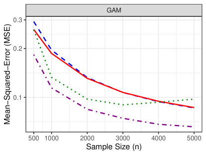
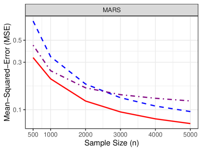
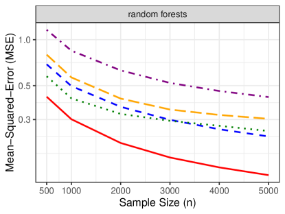
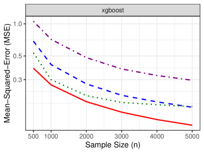
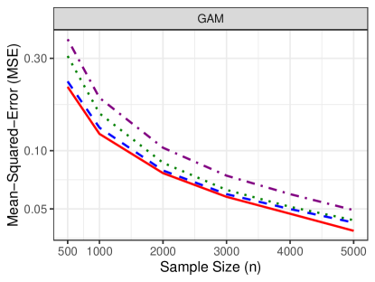
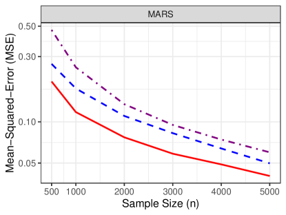
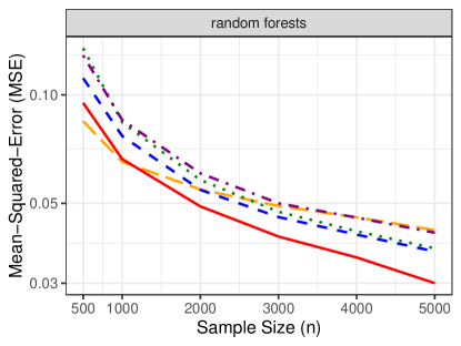
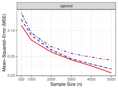
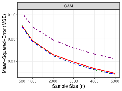
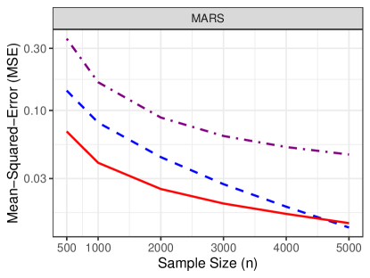
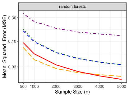
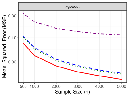
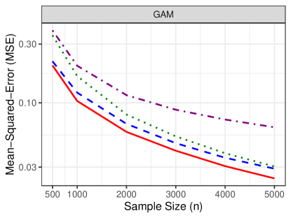
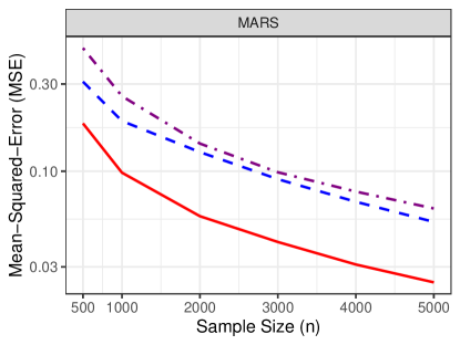
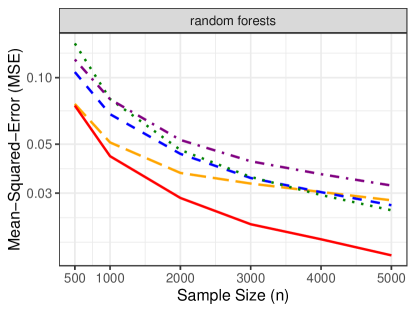
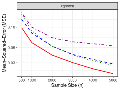
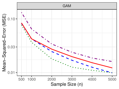
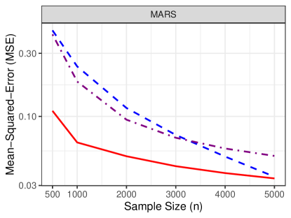
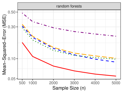
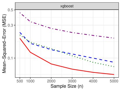
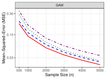
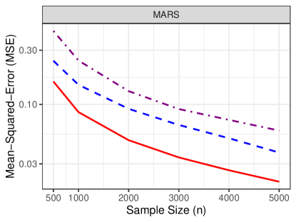
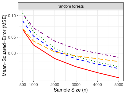
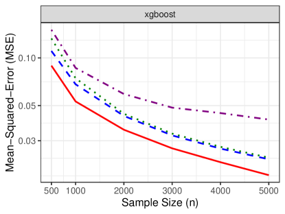
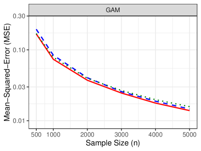
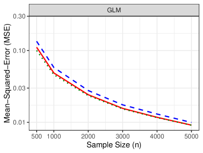
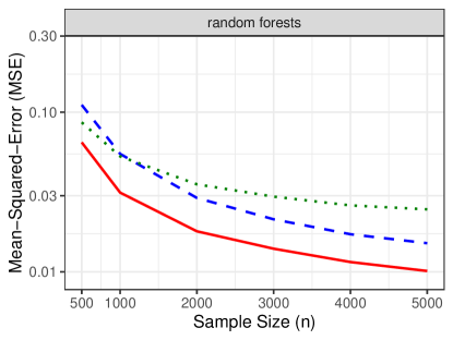
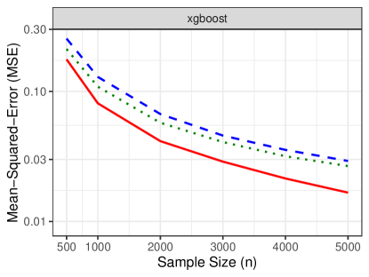
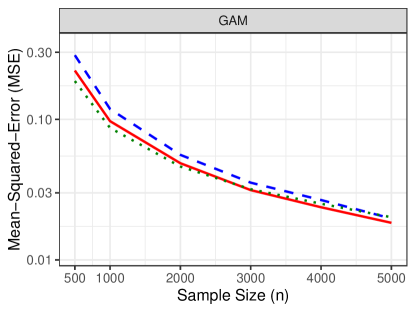
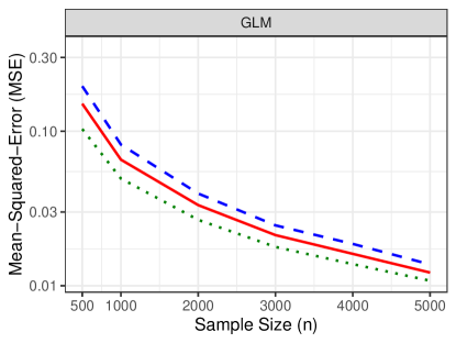
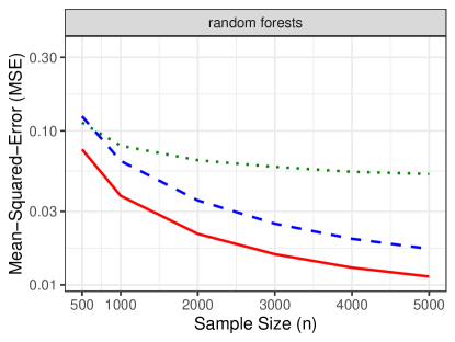
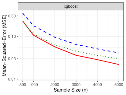
For each experimental setup and sample size $n\in\{500,1000,2000,3000,4000,5000\}$, we generated 1000 simulated datasets. The Monte Carlo empirical mean squared error was computed for each of the EP-learner and its competitors. Results for the CATE experiments with a complex functional form and moderate treatment overlap are displayed in Figure 3, whereas results for the log-CRR experiment with limited and moderate treatment overlap are shown in Figure 4. Results for simple causal contrasts and settings with limited treatment overlap are qualitatively similar and summarized in Appendix B.2.

(a) $d=3$

(b) $d=20$ with $5$ active

Figure 3: CATE experiments with a complex CATE and moderate treatment overlap: Mean squared error for DR-learner, R-learner, T-learner, and cross-validated EP-learner with supervised learning algorithm GAM, MARS, ranger, and xgboost. For the plots reporting the results of ranger, we also display the results of causal forests for comparison.

(a) Moderate treatment overlap

(b) Limited treatment overlap

Figure 4: CRR experiments with a complex CRR and moderate (left) and limited (right) treatment overlap: Mean-squared error for IPW-learner, T-learner, and CV-EP-learner with supervised learning algorithm GAM, random forests, and xgboost. The DR-learner algorithm for the CRR is not implemented due to nonconvexity of the loss.

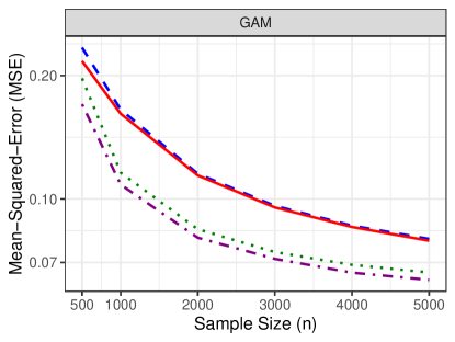
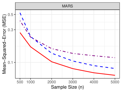
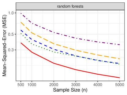
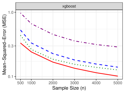
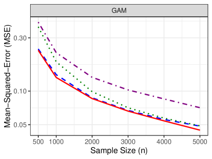
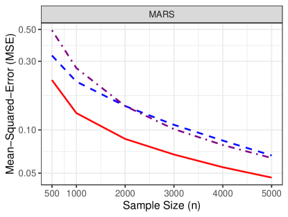
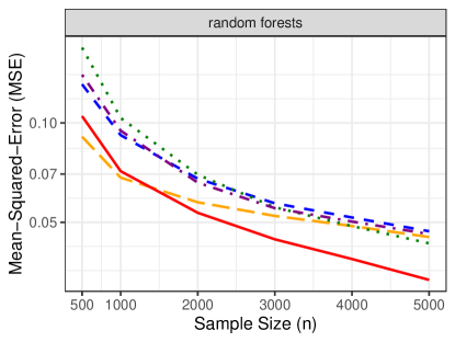
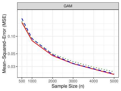
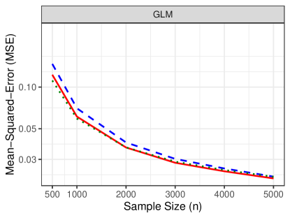
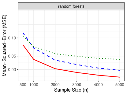
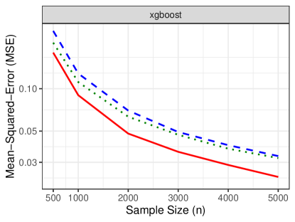
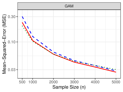
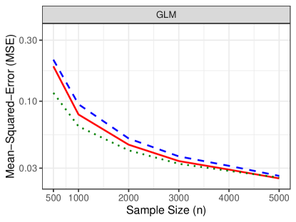
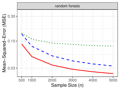
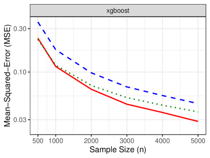
In all experimental settings and simulation scenarios, the EP-learner performed at least as well as — and in some cases, better than — all other methods considered. In the case of CATE learners based on generalized additive models, the EP-learner and DR-learner had comparable performance across all sample sizes. However, for more flexible algorithms, such as tree-based learners and MARS, the EP-learner significantly outperformed DR-learner in mean squared error across all settings, even for large sample sizes. For instance, in the CATE experiments with xgboost, the EP-learner reduced the mean squared error approximately three-fold compared to DR-learner at sample size $n=5000$. In all CATE experiments, R-learner and causal forests performed well. In the CATE experiment with covariate dimension $d=3$, the ranger and xgboost EP-learners exhibited better mean squared error than R-learner and causal forests across all settings and sample sizes. In the CATE experiment with covariate dimension $d=20$, causal forests slightly outperformed the ranger and xgboost EP-learners for smaller sample sizes, but the EP-learners perform best for larger sample sizes. In the log-CRR experiments, we found that the EP-learners generally performed as well or better than the T-learner, depending on the degree of treatment overlap. The IPW-learner exhibited significantly worse performance than the EP-learner in most settings.

7 Conclusion

In this work, we have introduced a framework for estimating a heterogeneous causal contrast based on a particular construction of an efficient plug-in risk function estimator. To the best of our knowledge, our construction gives the first doubly-robust, efficient estimator of a population risk function for the log-CRR function that corresponds to a convex loss function. While our primary focus has been on EP-learners for use in settings with a single time-point, discrete treatment, our framework can be extended to contexts involving continuous or longitudinal treatments. In future research, it would be of interest to explore the development of EP-learners for broader causal summaries, such as conditional treatment effects under longitudinal interventions (Luedtke et al., 2017, Rotnitzky et al., 2017). In contrast to the plug-in methods presented in these earlier works, the EP-learner would make it possible to leverage parsimony found in contrasts between counterfactual means under longitudinal interventions but otherwise not found in the counterfactual means themselves, for example.

To determine sieve specifications for the EP-learner, including basis function types and dimensions, we proposed using the cross-validated one-step risk estimator. In high-dimensional settings, defining a candidate basis for constructing a sieve can be challenging. In our simulation experiments, additive sieves based on univariate trigonometric series performed well, even with complex action spaces like random forests and boosted trees. However, incorporating tensor-product sieves with higher interaction degrees could potentially improve the performance of the EP-learner. Alternatively, it may be fruitful to data-adaptively learn a subset of variables that drive treatment effect heterogeneity and then use basis functions of those variables. In the case of estimating the covariate-adjusted conditional mean, Vansteelandt and Morzywołek (2023) proposes a penalized sieve method for constructing debiased plug-in risk estimators. Adapting our approach to incorporate penalization would be an interesting area for future work.

An unexplored application of the EP-learner is its potential to improve the calibration of predictors for the CATE through causal isotonic calibration (van der Laan et al., 2023). Isotonic calibration often exhibits poor calibration at the boundary of uncalibrated predictions, primarily because of overfitting of isotonic regression in that region (Groeneboom and Lopuhaa, 1993). However, this issue could be mitigated by utilizing an EP-learner risk estimator for the CATE, which would ensure that the pseudo-outcome employed for calibration itself serves as a CATE estimator.

Acknowledgements. Research reported in this publication was supported by NIH grants DP2-LM013340 and R01-HL137808, and NSF grant DMS-2210216. The content is solely the responsibility of the authors and does not necessarily represent the official views of the funding agencies.

Appendix A Code

An R package, hte3, implementing EP-learner can be found on GitHub here: https://github.com/Larsvanderlaan/hte3. Code to reproduce our experiments can be found here: https://github.com/Larsvanderlaan/hte3/tree/main/paper_EPlearner_experiments.

Appendix B Supplemental information for experiments

B.1 Small-scale experiments

Figure 5: (Left) Empirical reverse cumulative distribution function (RCDF) of estimated DR pseudo-outcome values for the simulated dataset. (Right) A zoomed in empirical RCDF. The 1% and 99% empirical quantiles of the pseudo-outcome are -3.2 and 3.1 while the maximum and minimum values are -16 and 14.

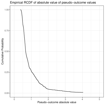
The following R code was used to generate the dataset corresponding to Figure 1. The code for running the analysis and generating the figures can be found at github/Larsvanderlaan/npcausalML/reproduceSims/introCATEFigure.R.

set.seed(12345)
n = 1500
W1 <- rt(n, df = 5)
pi0 <- plogis(W1)
A <- rbinom(n, 1, pi0)
mu0 =  0.35 + 0.65*plogis(W1-2 )
mu1 <- mu0 + plogis(2*W1+2) - plogis(W1-2) - 0.349
mu <- ifelse(A==1, mu1, mu0)
Y <- rbinom(n, 1, mu)
 

The following R code was used to generate the example dataset of Figure 2.

set.seed(123456)
n = 5
W1 <- rt(n, df = 5)
pi0 <- plogis(W1)
pi <- ifelse(A==1, pi0, 1-pi0)
A <- rbinom(n, 1, pi0)
mu0 =  0.35 + 0.65*plogis( W1-2 )
mu1 <- mu0 + plogis(2*W1+2) - plogis(W1-2) - 0.349
mu <- ifelse(A==1, mu1, mu0)
Y <- rbinom(n, 1, mu)
theta <- W1
weights <- round( (mu1 + mu0 + 1/pi*(Y - mu)),2)
outcome <- round((mu1  + A/pi0*(Y - mu1)) / weights,2)
dat <- data.frame(Covariate = round(W1,3), Weight  = weights, Outcome = outcome)
dat

B.2 Simulation design

For the low-dimensional CATE experiments, we consider $O=(W_{1},W_{2},W_{3},A,Y)$ for independent covariates $W_{1},W_{2},W_{3}$ each drawn from the uniform distribution on $(-1,+1)$. Given $W=w:=(w_{1},w_{2},w_{3})$, the treatment assignment $A$ was generated from a Bernoulli distribution with conditional mean defined, for the moderate overlap setting, as $\pi_{0}(1\,|\,w):=\text{expit}\left\{(w_{1}+w_{2}+w_{3})/3\right\}$ and, for the limited overlap setting, as $\pi_{0}(1\,|\,w):=\text{expit}\left\{w_{1}+w_{2}+w_{3}\right\}$. Given $(W,A)=(w,a)$, the outcome variable $Y$ was generated from a normal distribution with conditional mean $\mu_{0}(0,w)+a\cdot\theta_{0}^{-}(w)$ and variance $4$ where $\mu_{0}(0,w):=\sum_{k=1}^{3}\{w_{k}/2+\sin(5w_{k})+1/(w_{k}+1.2)\}$ and, in the simple setting, $\theta_{0}^{-}(w):=1+\sum_{k=1}^{3}w_{k}$ and, in the complex setting, $\theta_{0}^{-}(w):=1+\sum_{k=1}^{3}\{w_{k}+\sin(5w_{k})\}$.

For the high-dimensional CATE experiments, we generate $O=(W,A,Y)$ as follows. The covariate $W$ is drawn such that $W/2$ is distributed as a mean-zero multivariate truncated normal random variable with support $[-2,2]$, variances $1$, and covariances $0.4$. Given $W=w$, the treatment assignment $A$ was generated from a Bernoulli distribution with conditional mean $\pi_{0}(1\,|\,w)$ defined by $\text{logit}\{\pi_{0}(w)\}:=(1/1.3)(w_{1}+w_{5}+w_{9}+w_{11}+w_{19})$. Given $(W,A)=(w,a)$, the outcome variable $Y$ was generated from a normal distribution with conditional mean $\mu_{0}(0,w)+A\cdot\theta_{0}^{-}(w)$ and variance $4$ where $\mu_{0}(0,w)=(\cos(4w_{1})+\cos(4w_{5})+\sin(4w_{9})+1/(1.5+w_{15})+1/(1.5+w_{10}))/5$ and, in the simple setting, $\theta_{0}^{-}(w):=1+(w_{1}+w_{5}+w_{9}+w_{15}+w_{10})/5$ and, in the complex setting, $\theta_{0}^{-}(w):=1+(\sin(4w_{1})+\sin(4w_{5})+\cos(4w_{9})+1.5(w_{15}^{2}-w_{10}^{2}))/5$.

For the CRR experiments, we consider $O=(W_{1},W_{2},W_{3},A,Y)$ for independent covariates $W_{1},W_{2},W_{3}$ each drawn from the uniform distribution on $(-1,+1)$. Given $W=w$, the treatment assignment $A$ was generated from a Bernoulli distribution with conditional mean $\pi_{0}(1\,|\,w)$ where, in the moderate overlap setting, $\pi_{0}(1\,|\,w):=\text{expit}\left\{(w_{1}+w_{2}+w_{3})/3\right\}$ and, in the limited overlap setting, $\pi_{0}(1\,|\,w):=\text{expit}\left\{w_{1}+w_{2}+w_{3}\right\}$. Given $(W,A)=(w,a)$, the outcome variable $Y$ was generated from Bernoulli distribution with conditional mean $\mu_{0}(0,w)\exp\{a\theta_{0}^{\div}(w)\}$ where $\text{logit}\,\mu_{0}(0,w):=-1+0.3\sum_{k=1}^{3}w_{k}+\sin(4w_{k})$ and, in the simple setting, $\theta_{0}^{\div}(w):=-0.1+0.1\sum_{k=1}^{3}w_{k}$ and, in the complex setting, $\theta_{0}^{\div}(w):=-0.1+0.1\sum_{k=1}^{3}\{w_{k}+\sin(4w_{k})\}$.

B.3 Additional figures

(a) $d=3$, limited overlap

(b) $d=20$ with $5$ active, limited overlap

Figure 6: CATE experiments with a complex CATE and limited treatment overlap: Mean-squared error for DR-learner and CV-EP-learner with supervised learning algorithm GAM, MARS, ranger, and xgboost. For the plots reporting the results of tree-based algorithms (ranger and xgboost), we also display the results of causal forests for comparison. As a common benchmark across all learners, we display a cross-validated T-learner obtained from an ensemble library including xgboost and GAM learners.

(a) $d=3$, moderate overlap

(b) $d=20$ with $5$ active, moderate overlap

(c) $d=3$, limited overlap

(d) $d=20$ with $5$ active, limited overlap

Figure 7: CATE experiments with a simple CATE and moderate treatment overlap: Mean-squared error for DR-learner and CV-EP-learner with supervised learning algorithm GAM, MARS, ranger, and xgboost. For the plots reporting the results of tree-based algorithms (ranger and xgboost), we also display the results of causal forests for comparison. As a common benchmark across all learners, we display a cross-validated T-learner obtained from an ensemble library including xgboost and GAM learners.

(a) Moderate treatment overlap

(b) limited treatment overlap

Figure 8: CRR experiments with a simple CRR and moderate (left) and limited (right) treatment overlap: Mean-squared error for IPW-learner, T-learner, and CV-EP-learner with supervised learning algorithm GAM, random forests, and xgboost. The DR-learner algorithm for the CRR is not implemented due to nonconvexity of the loss.

Appendix C Additional details on EP-learner algorithm

C.1 Simplification of algorithm 1 for the CATE

When $h\circ\theta:=h_{1}\circ\theta=h_{2}\circ\theta$ for all $\theta\in\mathcal{F}$, the debiasing term $\frac{1}{n}\sum_{i=1}^{n}\Delta_{\pi_{n},\mu_{n}}(O_{i};\theta)$ in the general case simplifies to

$$\frac{1}{n}\sum_{i=1}^{n}\frac{1}{\pi_{n,j(i)}(A_{i}\,|\,W_{i})}\left\{\sum_{m\in\{1,2\}}H_{m,\mu_{n,j(i)}}(A_{i},W_{i})\right\}(h\circ\theta)(W_{i})\left\{Y_{i}-\mu_{n,j(i)}(A_{i},W_{i})\right\}.$$

In this setting, (6) is more than sufficient to make the debiasing term small. We can instead take the data-dependent feature vector in Algorithm 1 to be

$$\widehat{\varphi}_{k,j(i)}(a,w)=\left\{\sum_{m\in\{1,2\}}H_{m,\mu_{n,j(i)}}(A_{i},W_{i})\right\}\varphi_{k}(w).$$

With this modification, the resulting estimator $\mu_{n,k(n)}^{*}$ will, for all $\psi\in\mathcal{H}_{k(n)}$, satisfy

$$\frac{1}{n}\sum_{i=1}^{n}\frac{1}{\pi_{n,j(i)}(A_{i}\,|\,W_{i})}\left\{\sum_{m\in\{1,2\}}H_{m,\mu_{n,j(i)}}(A_{i},W_{i})\right\}\psi(W_{i})\left\{Y_{i}-\mu_{n,j(i)}^{*}(A_{i},W_{i})\right\}=0.$$

This modification halves the dimension of the sieve regressions of Algorithm 1 without any cost in the size of the debiasing term, and may lead to better finite-sample performance. In particular, for the CATE example, we recommend using $\widehat{\varphi}_{k,j(i)}(a,w)=(2a-1)\varphi_{k}(w)$, noting that $h_{1}\circ\theta=h_{2}\circ\theta=\theta$ and $\sum_{m\in\{1,2\}}H_{m,\mu_{n,j(i)}}(a,w)=2a-1$.

C.2 Debiasing method for general outcomes

Method 3: general outcomes (bound-preserving). $g(x)=\text{logit}\left((x-\widehat{a})/(\widehat{b}-\widehat{a})\right)$ where $\widehat{a}=\min\left\{Y_{i},\mu_{n,j(i)}(A_{i},X_{i}):i=1,\dots,n\right\}$ and $\widehat{b}=\max\left\{Y_{i},\mu_{n,j(i)}(A_{i},X_{i}):i=1,\dots,n\right\}$, and $\beta_{n}$ is the coefficient vector obtained from the the logistic regression of the $[0,1]$-transformed outcomes $((Y_{i}-\widehat{a})/(\widehat{b}-\widehat{a}):i\in[n])$ on the feature vectors $(\widehat{\varphi}_{k,j(i)}(A_{i},W_{i}):i\in[n])$ with offsets $\left(\text{logit}\left\{(\mu_{n,j(i)}(A_{i},W_{i})-\widehat{a})/(\widehat{b}-\widehat{a})\right\}:i\in[n]\right)$ and weights $\left(1/\pi_{n,j(i)}(A_{i}\,|\,W_{i}):i\in[n])\right)$. By construction, the sieve-adjusted estimates $\mu_{n,j(i)}(A_{i},W_{i})$ lie in $[\widehat{a},\widehat{b}]$.

Appendix D Uniform consistency of the fixed $K$-nearest neighbors EP-learner

Consider the estimation of the conditional average treatment effect based on the population risk function given in Section 3.1. Suppose that $W$ is uniformly distributed on the hypercube $(0,1)^{d}$. Let $\mu_{n}^{*}$ be a debiased outcome regression estimator obtained from initial estimators $\pi_{n}$ and $\mu_{n}$ of $\pi_{0}$ and $\mu_{0}$ using Algorithm 1 where, for simplicity, we study a method that does not use cross-fitting, so that $\pi_{n,j}=\pi_{n}$ and $\mu_{n,j}=\mu_{n}$ for each $j\in[J]$. Let $\theta_{n,EP}$ be the EP-learner obtained from Algorithm 2 using $K$-nearest neighbors for some fixed $K\in\mathbb{N}$ under the Euclidean norm. For each $w\in(0,1)^{d}$, the EP-learner can be expressed pointwise as $\theta_{n,EP}(w)=\frac{1}{K}\sum_{i=1}^{n}1(i\in\mathcal{I}_{K,n}(w))\left[\mu_{n}^{*}(1,W_{i})-\mu_{n}^{*}(0,W_{i})\right]$, where $\mathcal{I}_{K,n}(w)$ are the observation indices for the $K$ nearest observations to $x$ under the Euclidean norm, with ties broken arbitrarily. The following theorem establishes that the EP-learner is, for any $K\in\mathbb{N}$ including $K=1$, uniformly consistent for the CATE $\theta_{0}^{-}$ so long as the T-learner obtained from $\mu_{n}^{*}$ is uniformly consistent. In contrast, DR-learner is generally inconsistent if the number of neighbors $K$ is held fixed with sample size $n$.

Theorem 6.

Suppose $W$ is uniformly distributed on the hypercube $[0,1]^{d}$ and that $\mu_{0}$ is Lipschitz-continuous on $\{0,1\}\times[0,1]^{d}$. Let the number of neighbors $K\in\mathbb{N}$ be fixed. Then,

$$\sup_{w\in(0,1)^{d}}\left|\theta_{n,EP}(w)-\theta_{0}^{-}(w)\right|\lesssim\sup_{w\in(0,1)^{d}}\left|\mu_{n}^{*}(1,w)-\mu_{n}^{*}(0,w)-\theta_{0}^{-}(w)\right|+O_{p}\left((K\log n/n)^{1/d}\right).$$

Proof of Theorem 6.

For now fix $w\in(0,1)^{d}$. Let $B_{K,n}(w)$ be the smallest closed ball centered at $x$ that contains $\{W_{i}:i\in\mathcal{I}_{K,n}(w)\}$. We work on the probability 1 event where the set of $K$ nearest neighbors $\mathcal{I}_{K,n}(w)$ is uniquely specified, that is, there are no ties. On this event, $W_{i}\in B_{K,n}(w)$ if and only if $i\in\mathcal{I}_{K,n}(w)$. Denote $w\mapsto\theta_{n,T}^{*}(w)=\mu_{n}^{*}(1,w)-\mu_{n}^{*}(0,w)$ as the T-Learner obtained from $\mu_{n}^{*}$. We have

$$\left|\theta_{n,EP}(w)-\theta_{0}(w)\right| =\left|\frac{1}{K}\sum_{i=1}^{n}1(i\in\mathcal{I}_{K,n}(w))\left[\mu_{n}^{*}(1,W_{i})-\mu_{n}^{*}(0,W_{i})-\left\{\mu_{0}(1,w)-\mu_{0}(0,w)\right\}\right]\right|$$

$$=\left|\frac{1}{K}\sum_{i=1}^{n}1(W_{i}\in B_{K,n}(w))\left[\mu_{n}^{*}(1,W_{i})-\mu_{n}^{*}(0,W_{i})-\left\{\mu_{0}(1,w)-\mu_{0}(0,w)\right\}\right]\right|$$

$$\leq\left|\frac{1}{K}\sum_{i=1}^{n}1(W_{i}\in B_{K,n}(w))\left[\mu_{n}^{*}(1,W_{i})-\mu_{n}^{*}(0,W_{i})-\left\{\mu_{0}(1,W_{i})-\mu_{0}(0,W_{i})\right\}\right]\right|$$

$$\quad+\left|\frac{1}{K}\sum_{i=1}^{n}1(W_{i}\in B_{K,n}(w))\left[\mu_{0}(1,W_{i})-\mu_{0}(0,W_{i})-\left\{\mu_{0}(1,w)-\mu_{0}(0,w)\right\}\right]\right|$$

$$\lesssim\|\theta_{n,T}^{*}-\theta_{0}^{-}\|_{\infty}+\sup_{w^{\prime}\in(0,1)^{d},a\in\{0,1\}}\sup_{x\in B_{K,n}(w^{\prime})}\left|\mu_{0}(a,x)-\mu_{0}(a,x)\right|$$

$$\lesssim\|\theta_{n,T}^{*}-\theta_{0}^{-}\|_{\infty}+\sup_{w^{\prime}\in(0,1)^{d}}\sup_{x\in B_{K,n}(w^{\prime})}L\|x-w^{\prime}\|_{2},$$

where $L$ denotes the Lipschitz constant of $\mu_{0}$. Since the right-hand side does not depend on the choice of $w\in(0,1)^{d}$, we can take a supremum over this quantity on the left-hand side to show that

$$\sup_{w\in(0,1)^{d}}\left|\theta_{n,EP}(w)-\theta_{0}^{-}(w)\right| \lesssim\|\theta_{n,T}^{*}-\theta_{0}^{-}\|_{\infty}+\sup_{w^{\prime}\in(0,1)^{d}}\sup_{x\in B_{K,n}(w^{\prime})}L\|x-w^{\prime}\|_{2},$$

By Corollary 1.5 of Chenavier et al. (2022), the maximal volume of the ball $B_{K,n}(w^{\prime})$ over $w^{\prime}\in(0,1)^{d}$ is $O_{p}(K\log n/n)$. This implies that the maximal radius of $B_{K,n}(w^{\prime})$ over $w^{\prime}\in(0,1)^{d}$ is of the order $O_{p}\left((K\log n/n)^{1/d}\right)$, up to a constant depending on $d$. Hence, the latter term on the right-hand side above is $O_{p}\left((K\log n/n)^{1/d}\right)$, which gives the desired result. ∎

Appendix E Preliminaries for proofs

E.1 Notation and conventions for proofs

For two quantities $x$ and $y$, we use the expression $x\lesssim y$ to mean that $x$ is upper bounded by $y$ times a universal constant that may only depend on global constants, including $\eta$, $M$, and $C$, that appear the conditions of Theorems 2-5.

For a function class $\mathcal{F}$, we denote its norms by $\|\mathcal{F}\|:=\sup_{f\in\mathcal{F}}\|f\|$ and $\|\mathcal{F}\|_{\infty}:=\sup_{f\in\mathcal{G}}\|f\|_{\infty}$. For a uniformly bounded function class $\mathcal{F}$ and distribution $P$, let $N(\epsilon,\mathcal{F},L_{2}(P))$ denote the $\varepsilon-$covering number (van der Vaart and Wellner, 1996) of $\mathcal{F}$ with respect to the $L_{2}(P)$-metric. We define the uniform entropy integral of $\mathcal{F}$ by

$$\mathcal{J}(\delta,\mathcal{F}):=\int_{0}^{\delta}\sup_{Q}\sqrt{\log N(\varepsilon,\mathcal{F},L_{2}(Q))}\,d\varepsilon\ ,$$

where the supremum is taken over all discrete probability distributions $Q$.

In our proofs, we use the following notation. We let $\mathbb{I}_{g_{1},g_{2}}$ be the indicator that takes the value $0$ if both $g_{1}$ and $g_{0}$ are the identity function. We denote the nuisance rates:

$$r_{n}^{*} :=n^{-\beta/(2\beta+1)}+\sqrt{k(n)\log n/n};$$

$$s_{n}^{*} :=r_{n}^{*}+n^{-\gamma/(2\gamma+1)}.$$

We denote, for each $P\in\mathcal{M}$, the Neyman orthogonal loss function corresponding with $R_{P}$ by $L_{\pi_{P},\mu_{P}}:=L_{\mu_{P}}+\Delta_{\pi_{P},\mu_{P}}$. For $\phi\in L^{2}(P_{0,W})$, $j\in[J]$, and $m\in\{1,2\}$, we define pointwise, for $o\in\mathcal{O}$, the following variants of the debiasing term:

$$\overline{\Delta}^{(m)}_{\pi_{n,j},\mu_{n,j}^{*}}(o\,,\phi):=\frac{1}{\pi_{n,j}(a\,|\,w)}\left\{H_{m,\mu_{n,j}^{*}}(a,w)\cdot\phi(w)\right\}\left\{y-\mu_{n,j}^{*}(a,w)\right\};$$

$$\overline{\Delta}^{*(m)}_{\pi_{n,j},\mu_{n,j}}(o\,,\phi):=\frac{1}{\pi_{n,j}(a\,|\,w)}\left\{H_{m,\mu_{n,j}}(a,w)\cdot\phi(w)\right\}\left\{y-\mu_{n,j}^{*}(a,w)\right\}.$$

The overline encodes dependence on the transformed action-space $\mathcal{H}$ as opposed to the original action-space $\mathcal{F}$. The superscript by $*$ encodes that the residual in the definition corresponds to the debiased outcome regression estimator.

Recall $\{\mathcal{D}_{n}^{j}:j\in[J]\}$ is the partitioning of $\mathcal{D}_{n}:=\{O_{i}:i\in[n]\}$ used for cross-fitting the initial nuisance estimators, $\{\mu_{n,j},\pi_{n,j}:j\in[J]\}$, as in Algorithm 3. We define the $j$-th training set $\mathcal{T}_{n}^{j}:=\mathcal{D}_{n}\backslash\mathcal{D}_{n}^{j}$. We let $P_{n,j}$ denote the empirical distribution of the $j$th data-fold $\mathcal{D}_{n}^{j}$ and define the fold-specific empirical process operator $f\mapsto P_{n,j}f:=\int f(o)dP_{n,j}(o)$. For ease of presentation, we will use the following cross-fitting notation. For a collection of fold-specific functions $\nu_{n,\diamond}:=\{\nu_{n,j}:j\in[J]\}$ that may depend on $n$, we define the fold-averaged empirical process operators:

$$\overline{P}_{0}\nu_{n,\diamond} :=\frac{1}{J}\sum_{j=1}^{J}P_{0}\nu_{n,j};$$

$$\overline{P}_{n}\nu_{n,\diamond} :=\frac{1}{J}\sum_{j=1}^{J}P_{n,j}\nu_{n,j}.$$

We define the fold-averaged norm of a collection of fold-specific functions $\nu_{\diamond}:=\{\nu_{j}:j\in[J]\}$ as $\|\nu_{\diamond}\|_{\overline{P}_{0}}:=\sqrt{\frac{1}{J}\sum_{j=1}^{J}\|\nu_{j}\|^{2}_{P_{0}}}$. For a function $h:\mathbb{R}\rightarrow\mathbb{R}$, we also define the composition $h\circ\nu_{\diamond}:=\{h\circ\nu_{j}:j\in[J]\}$. The above notation lets us treat the collection of debiased cross-fitted estimators $\mu_{n,\diamond}^{*}:=\{\mu_{n,j}^{*}:j\in[J]\}$ as extended functions defined on $\mathcal{A}\times\mathcal{W}\times[J]$. For example, in our proofs, $\overline{P}_{n}\overline{\Delta}^{(m)}_{\pi_{n,\diamond},\mu_{n,\diamond}^{*}}(\cdot,\phi)$ is notation for $J^{-1}\sum_{j\in[J]}\int\overline{\Delta}^{(m)}_{\pi_{n,j},\mu_{n,j}^{*}}(o,\phi)dP_{n,j}(o)$.

In our proofs, for some sufficiently large $M>0$, we will work on the following events:

1. $\max_{j\in[J]}\left\lVert\mu_{n,j}-\mu_{0}\right\rVert\leq Mn^{-\beta/(2\beta+1)}$

2. $\max_{j\in[J]}\left\lVert\pi_{n,j}-\pi_{0}\right\rVert\leq Mn^{-\gamma/(2\gamma+1)}$

3. $\max_{j\in[J]}\left\lVert\mu_{n,j}^{*}-\mu_{0}\right\rVert\leq Mn^{-\beta/(2\beta+1)}+M\sqrt{k(n)\log n/n}$.

4. $\left\lVert\beta_{n}\right\rVert_{\infty}\leq M$.

Let $A_{n}$ be the union of events E1-E4, and let $\mathbb{I}_{A_{n}}$ denote the indicator that event $A_{n}$ occurs. In our proofs, we will choose $M>0$ so that the event $A_{n}$ occurs asymptotically with probability at least $1-\varepsilon$. We claim, under C2 and C1b, that we can always choose such an $M>0$. To see this, note, under condition C2, we can take $M$ large enough so that events E1-E3 occur asymptotically with probability arbitrarily close to one. Under Condition C1b, we claim that Event E4 occurs with probability tending to one. To show this, recall by definition that $\mu_{n,j(i)}^{*}=g^{-1}(g(\mu_{n,j(i)})+\widehat{\varphi}_{k(n),i}^{T}\beta_{n})$. By C1b, we have that $\mu_{n,j(i)}$ and $\mu_{n,j(i)}^{*}$ are bounded with probability tending to one and, since the feature mapping $\varphi_{k(n)}$ is bounded by definition, $\widehat{\varphi}_{k(n),i}$ is bounded with probability tending to one. Since $g$ is a continuous invertible function, we have that $\beta_{n}$ must also be bounded with probability tending to one. The claim then follows taking $M>0$ large enough so that $\left\lVert\beta_{n}\right\rVert_{\infty}\leq M$ with probability tending to one.

E.2 Supporting Lemmas and empirical process bounds

In this section, we present some technical lemmas used to bound empirical process remainders and second-order bias terms that appear in our proofs.

The following lemma due to Belloni et al. (2012) bounds the sup-norm sieve approximation error of the $L^{2}(P_{0})$-projection $\Pi_{k(n)}$. For the following lemma, we define the rate $\rho_{n,\infty}:=\{\log k(n)\}^{\nu}k(n)^{-\rho}$.

Lemma 1.

Under C3a and C3b, it holds that

$$\sup_{\phi\in\mathcal{H}}\|\phi-\Pi_{k(n)}\phi\|_{\infty} \lesssim\{\log k(n)\}^{\nu}\sup_{\phi\in\mathcal{H}}\inf_{f\in\mathcal{H}_{k(n)}}\|\phi-f\|_{\infty}\lesssim\rho_{n,\infty}.$$

Proof.

Condition C3a and Proposition 3.2. of Belloni et al. (2012) imply that $\sup_{\phi\in\mathcal{H}}\|\phi-\Pi_{k(n)}\phi\|_{\infty}\lesssim(\log k(n))^{\nu}\sup_{\phi\in\mathcal{H}}\inf_{f\in\mathcal{H}_{k(n)}}\|\phi-f\|_{\infty}$. The second bound then follows from C3b, noting that $\sup_{\phi\in\mathcal{H}}\inf_{f\in\mathcal{H}_{k(n)}}\|\phi-f\|_{\infty}\lesssim k(n)^{-\rho}$. ∎

Lemma 2.

Let $\mathcal{F}_{1},\dots,\mathcal{F}_{k}$ be given uniformly bounded function classes with $\mathcal{J}_{\infty}(1,\mathcal{F}_{j})<\infty$ for each $j\in[k]$. Let $\varphi:\mathbb{R}^{k}\rightarrow\mathbb{R}$ by a Lipschitz-continuous map. Then, the function class $\mathcal{G}:=\left\{\varphi(f_{1},\dots,f_{k}):(f_{1},\dots,f_{k})\in\mathcal{F}_{1}\times\dots\times\mathcal{F}_{k}\right\}$ satisfies $\log N_{\infty}(\varepsilon,\mathcal{G})\lesssim\sum_{j=1}^{k}\log N_{\infty}(\varepsilon,\mathcal{F}_{j})$ and, hence, $\mathcal{J}_{\infty}(\delta,\mathcal{G})\lesssim\sum_{j=1}^{k}\mathcal{J}_{\infty}(\delta,\mathcal{F}_{j})$.

Proof.

This result follows from the proof of Theorem 2.10.20 in van der Vaart and Wellner (1996). ∎

The following lemma relates the sup-norm entropy integral of $\mathcal{H}$ to those of the function classes $\mathcal{H}-\Pi_{k}\mathcal{H}:=\{\phi-\Pi_{k}\phi:\phi\in\mathcal{H}\}$ and $\Pi_{k}\mathcal{H}:=\{\Pi_{k}\phi:\phi\in\mathcal{H}\}$.

Lemma 3.

Under C3 and C4, we have, for all $\delta>0$, that $\mathcal{J}_{\infty}(\delta,\mathcal{H})\lesssim\mathcal{J}_{\infty}(\delta,\mathcal{F})$, $\mathcal{J}_{\infty}(\delta,\Pi_{k}\mathcal{H})\lesssim\mathcal{J}_{\infty}(\{\log k(n)\}^{\nu}\delta,\mathcal{F})$, and $\mathcal{J}_{\infty}(\delta,\mathcal{H}-\Pi_{k}\mathcal{H})\lesssim\mathcal{J}_{\infty}(\{\log k(n)\}^{\nu}\delta,\mathcal{F})$

Proof.

Recall, by definition, that $\mathcal{H}:=\{h_{i}\circ\theta:\theta\in\mathcal{F},i\in\{1,2\}\}$ where $h_{1}$ and $h_{2}$ are Lipschitz-continuous functions. Thus, by Lemma 2, we have $\mathcal{J}_{\infty}(\delta,\mathcal{H})\lesssim\mathcal{J}_{\infty}(\delta,\mathcal{F})$. Now, for $i\in\{1,2\}$, let $(\phi_{i}-\Pi_{k}\phi_{i})$ be an element of $\mathcal{H}-\Pi_{k}\mathcal{H}$. Using linearity of the $L^{2}(P_{0})$-projection and the Lebesgue constant bound of C3a, we have

$$\|(\Pi_{k}\phi_{1})-\Pi_{k}\phi_{2}\|_{\infty} =\|\Pi_{k}(\phi_{1}-\phi_{2})\|_{\infty}$$

$$\lesssim\{\log k(n)\}^{\nu}\|\phi_{1}-\phi_{2}\|_{\infty}.$$

Thus, $\Pi_{k}\mathcal{H}=\{\Pi_{k}\phi:\phi\in\mathcal{H}\}$ is, relative to the sup-norm, a Lipschitz transformation of the function class $\mathcal{H}$ with Lipschitz constant equal to $C\{\log k(n)\}^{\nu}$ for some constant $C>0$. Hence, we have $\log N_{\infty}(\varepsilon,\mathcal{H}_{k})\lesssim\log N_{\infty}(\{\log k(n)\}^{\nu}\varepsilon,\mathcal{H})$ and, therefore, by Lemma 2, $\log N_{\infty}(\varepsilon,\mathcal{H}_{k})\lesssim\log N_{\infty}(\{\log k(n)\}^{\nu}\varepsilon,\mathcal{F})$. It then follows, from a change of variables, that

$$\mathcal{J}_{\infty}(\delta,\Pi_{k}\mathcal{H}) =\int_{0}^{\delta}\sqrt{\log N_{\infty}(\varepsilon,\mathcal{H}_{k})}d\varepsilon$$

$$\lesssim\int_{0}^{\delta}\sqrt{\log N_{\infty}(\{\log k(n)\}^{\nu}\varepsilon,\mathcal{F})}d\varepsilon$$

$$=\{\log k(n)\}^{-\nu}\int_{0}^{\{\log k(n)\}^{\nu}\delta}\sqrt{\log N_{\infty}(\varepsilon,\mathcal{F})}d\varepsilon$$

$$=\{\log k(n)\}^{-\nu}\mathcal{J}_{\infty}(\{\log k(n)\}^{\nu}\delta,\mathcal{F}).$$

Since $\{\log k(n)\}^{-\nu}=O(1)$ as $\nu\geq 0$, we have $\mathcal{J}_{\infty}(\delta,\Pi_{k}\mathcal{H})\lesssim\mathcal{J}_{\infty}(\{\log k(n)\}^{\nu}\delta,\mathcal{F})$, as desired. Finally, observe that $\mathcal{H}-\mathcal{H}_{k}$ is a Lipschitz transformation of $\mathcal{H}$ and $\mathcal{H}_{k}$. Thus, by Lemma 2, we have $\mathcal{J}_{\infty}(\delta,\mathcal{H}-\Pi_{k}\mathcal{H})\lesssim\mathcal{J}_{\infty}(\delta,\mathcal{H})+\mathcal{J}_{\infty}(\delta,\Pi_{k}\mathcal{H})\lesssim\mathcal{J}_{\infty}(\{\log k(n)\}^{\nu}\delta,\mathcal{F})$, where the final inequality follows from our earlier claims.

∎

The next lemmas provide local maximal inequalities for empirical processes in terms of the sup-norm metric entropy integral. The following lemma is a restatement of Theorem 2.1. in van de Geer (2014).

Lemma 4.

Suppose $\mathcal{J}_{\infty}(\infty,\mathcal{F})<\infty$. Then, $\sqrt{E\left\lVert\mathcal{F}\right\rVert_{P_{n}}^{2}}\lesssim\left\lVert\mathcal{F}\right\rVert+\frac{\mathcal{J}_{\infty}\left(\left\lVert\mathcal{F}\right\rVert_{\infty},\mathcal{F}\right)}{\sqrt{n}}$ and, as such,

$$E\left[\sup_{f\in\mathcal{F}}\left|(P_{n}-P)f\right|\right]\lesssim n^{-1/2}\mathcal{J}_{\infty}\left(\delta,\mathcal{F}\right),$$

for any $\delta\geq\left\lVert\mathcal{F}\right\rVert+n^{-1/2}$ .

The following lemmas provide local maximal inequalities for function classes obtained by taking the pointwise product of elements of two function classes. The first lemma follows from a modification of the proof of Theorem 2.1 in Van Der Vaart and Wellner (2011) where, in Equation (2.2) of their proof, we argue as in the proof of Theorem 3.1 of van de Geer (2014). In the following, let $\mathcal{H}$ and $\mathcal{G}$ be two uniformly bounded function classes. Denote the class obtained by taking pointwise products of their respective elements as $\mathcal{H}\mathcal{G}:=\{hg:h\in\mathcal{H},g\in\mathcal{G}\}$.

Lemma 5.

Suppose $\mathcal{J}_{\infty}(1,\mathcal{H})<\infty$ and $\mathcal{J}(1,\mathcal{G})<\infty.$ Then,

$$E\left\lVert\mathbb{G}_{n}\right\rVert_{\mathcal{G}\mathcal{H}}\lesssim\sqrt{E\left\lVert\mathcal{G}\right\rVert_{P_{n}}^{2}}\mathcal{J}_{\infty}\left(\sqrt{E\left\lVert\mathcal{H}\mathcal{G}\right\rVert_{P_{n}}^{2}}/\sqrt{E\left\lVert\mathcal{G}\right\rVert_{P_{n}}^{2}},\mathcal{H}\right)+\left\lVert\mathcal{H}\right\rVert_{\infty}\mathcal{J}\left(\sqrt{E\left\lVert\mathcal{H}\mathcal{G}\right\rVert_{P_{n}}^{2}}/\left\lVert\mathcal{H}\right\rVert_{\infty},\mathcal{G}\right).$$

Furthermore, $\sqrt{E\left\lVert\mathcal{H}\mathcal{G}\right\rVert_{P_{n}}^{2}}\lesssim\left\lVert\mathcal{G}\right\rVert_{\infty}\max\left(\left\lVert\mathcal{H}\right\rVert_{P_{0}},\frac{\mathcal{J}_{\infty}(\left\lVert\mathcal{H}\right\rVert_{\infty},\mathcal{H})}{\sqrt{n}}\right)$ and, for any $\delta_{crit,\mathcal{G}}>0$ satisfying $\sqrt{n}\delta_{crit,\mathcal{G}}^{2}\geq\left\lVert\mathcal{G}\right\rVert_{\infty}\mathcal{J}(\delta_{crit,\mathcal{G}}/\left\lVert\mathcal{G}\right\rVert_{\infty},\mathcal{G})$, it holds that $\sqrt{E\left\lVert\mathcal{H}\mathcal{G}\right\rVert_{P_{n}}^{2}}\lesssim\left\lVert\mathcal{H}\right\rVert_{\infty}\max\left(\left\lVert\mathcal{G}\right\rVert_{P_{0}},\delta_{crit,\mathcal{G}}\right)$.

Proof.

For a function class $\mathcal{F}$, let $\mathcal{J}_{n}(\delta,\mathcal{F}):=\int_{0}^{\delta}\sqrt{\log N(\varepsilon,\mathcal{F},\|\cdot\|_{P_{n}})}d\varepsilon$. By Dudley’s inequality (Equation 2.1 of Theorem 2.1 in Van Der Vaart and Wellner (2011)), it holds, for $\delta_{n}:=\|\mathcal{G}\mathcal{H}\|_{P_{n}}$, that

$$E\left\lVert\mathbb{G}_{n}\right\rVert_{\mathcal{G}\mathcal{H}}\lesssim E\left[\mathcal{J}_{n}(\delta_{n},\mathcal{G}\mathcal{H})\right].$$

Since $\|g_{1}h_{1}\|_{P_{n}}-\|g_{2}h_{2}\|_{P_{n}}\leq\|h_{1}-h_{2}\|_{\infty}\|g_{1}\|_{P_{n}}+\|g_{1}-g_{2}\|_{P_{n}}\|\|h_{2}\|_{\infty}$, it holds that

$$\log N(\varepsilon,\mathcal{G}\mathcal{H},\|\cdot\|_{P_{n}})\lesssim\log N(\varepsilon/\|\mathcal{H}\|_{\infty},\mathcal{G},\|\cdot\|_{P_{n}})+\log N_{\infty}(\varepsilon/\|\mathcal{G}\|_{P_{n}},\mathcal{G}),$$

and, hence,

$$\mathcal{J}_{n}(\delta,\mathcal{G}\mathcal{H}) =\int_{0}^{\delta}\sqrt{\log N(\varepsilon,\mathcal{G}\mathcal{H},\|\cdot\|_{P_{n}})}d\varepsilon$$

$$\lesssim\int_{0}^{\delta}\sqrt{\log N(\varepsilon/\|\mathcal{H}\|_{\infty},\mathcal{G},\|\cdot\|_{P_{n}})}d\varepsilon+\int_{0}^{\delta}\sqrt{\log N_{\infty}(\varepsilon/\|\mathcal{G}\|_{P_{n}},\mathcal{H})}d\varepsilon$$

$$\lesssim\|\mathcal{H}\|_{\infty}\mathcal{J}(\delta/\|\mathcal{H}\|_{\infty},\mathcal{G})+\|\mathcal{G}\|_{P_{n}}\mathcal{J}_{\infty}(\delta/\|\mathcal{G}\|_{P_{n}},\mathcal{H}).$$

Thus, the identity $E\left\lVert\mathbb{G}_{n}\right\rVert_{\mathcal{G}\mathcal{H}}\lesssim E\left[\mathcal{J}_{n}(\delta_{n},\mathcal{G}\mathcal{H})\right]$ implies that

$$E\left\lVert\mathbb{G}_{n}\right\rVert_{\mathcal{G}\mathcal{H}}\lesssim E\left[\|\mathcal{H}\|_{\infty}\mathcal{J}(\delta_{n}/\|\mathcal{H}\|_{\infty},\mathcal{G})\right]+E\left[\|\mathcal{G}\|_{P_{n}}\mathcal{J}_{\infty}(\delta_{n}/\|\mathcal{G}\|_{P_{n}},\mathcal{H})\right].$$

As in the proof of Theorem 2.1 of Van Der Vaart and Wellner (2011), concavity of the maps $(x,y)\mapsto\sqrt{y}\mathcal{J}_{\infty}(\sqrt{x/y},\mathcal{H})$ and Jenson’s inequality implies that

$$E\left\lVert\mathbb{G}_{n}\right\rVert_{\mathcal{G}\mathcal{H}}\lesssim\|\mathcal{H}\|_{\infty}\mathcal{J}(\sqrt{E\delta_{n}^{2}}/\|\mathcal{H}\|_{\infty},\mathcal{G})+\sqrt{E\|\mathcal{G}\|_{P_{n}}^{2}}\mathcal{J}_{\infty}(\sqrt{E\delta_{n}^{2}}/\sqrt{E\|\mathcal{G}\|_{P_{n}}^{2}},\mathcal{H}).$$

The first bound then follows from the definition of $\delta_{n}$. The remaining norm bounds are an immediate consequence of Theorem 2.1 and Theorem 2.2 in van de Geer (2014).

∎

The following lemma is an immediate corollary of the above lemma and is used directly in our proofs.

Lemma 6.

Let ${\mathcal{H}}$ be a uniformly bounded function class satisfying $\mathcal{J}_{\infty}(\infty,{\mathcal{H}})<\infty$ and let $\mathcal{G}$ be a function class with $\mathcal{J}(\delta,\mathcal{G})\lesssim\delta\sqrt{k(n)\log(1/\delta)}$ where $\log(1/\left\lVert\mathcal{G}\right\rVert)+\log(1/\left\lVert\mathcal{H}\right\rVert)=O(1/\log n)$. Then,

$$E\left\lVert\mathbb{G}_{n}\right\rVert_{{\mathcal{H}}\mathcal{G}}\lesssim \left\lVert\mathcal{G}\right\rVert_{P_{0}}\mathcal{J}_{\infty}\left(\max\left\{\left\lVert\mathcal{H}\right\rVert_{P_{0}},n^{-1/2}\right\}/\left\lVert\mathcal{G}\right\rVert_{P_{0}},\mathcal{H}\right)$$

$$\quad+\left\lVert\mathcal{H}\right\rVert_{\infty}\sqrt{k(n)\log n}\cdot\max\left\{\left\lVert\mathcal{G}\right\rVert_{P_{0}},\sqrt{k(n)\log n/n}\right\}.$$

Appendix F Statement and proofs of technical lemmas

F.1 Lemmas bounding key excess risk remainder terms

In this section, we use the supporting lemmas of Appendix E.2 to obtain bounds for various remainder terms that appear in our proofs.

The following lemma demonstrates that Lipschitz transformations of the debiased outcome regression estimator $\mu_{n,j}^{*}$, where $j\in[J]$, falls in function class that is, deterministic conditional on the training set $\mathcal{D}_{n}\backslash\mathcal{D}_{n}^{j}$, and has uniform entropy integral at $\delta>0$ scaling as $\delta\sqrt{k(n)\log(1/\delta)}$.

Lemma 7.

Assume Condition C1 and work on the good events E1, E3, and E4. Let $T_{n,j}:\mathbb{R}\rightarrow\mathbb{R}$ be a uniformly bounded $L$-Lipschitz continuous function that is deterministic conditional on the data-fold $\mathcal{D}_{n}\backslash\mathcal{D}_{n}^{j}$. There exists a uniformly bounded random function class $\mathcal{E}_{n,j}$ with the following properties on the good events. (i) $T_{n,j}(\mu_{n,j^{*}})-T_{n,j}(\mu_{0})$ and $T_{n,j}(\mu_{n,j^{*}})-T_{n,j}(\mu_{n,j})$ fall in $\mathcal{E}_{n,j}$ almost surely; (ii) $\mathcal{E}_{n,j}$ is deterministic conditional on $\mathcal{D}_{n}\backslash\mathcal{D}_{n}^{j}$; (iii) $\left\lVert\mathcal{E}_{n,j}\right\rVert\lesssim LMn^{-\beta/(2\beta+1)}+LM\sqrt{k(n)\log n/n}$; and (iv) $\mathcal{J}(\delta,\mathcal{E}_{n,j})\lesssim\delta\sqrt{k(n)\log(1/\delta)}$.

Proof of Lemma 7.

We work on Events E1, E3, and E4. By construction, as shown in Algorithm 1, we have the expression $\mu_{n,j}^{*}=g^{-1}(g\circ\mu_{n,j}+\widehat{\varphi}_{k(n),j}^{\top}\beta_{n})$, where $\mu_{n,j}^{*}$ depends randomly only through $\beta_{n}\in\mathbb{R}^{2k(n)}$, conditional on $\mathcal{D}_{n}\backslash\mathcal{D}_{n}^{j}$. Assuming C1 and on Event E4, the mapping $(a,w)\mapsto\widehat{\varphi}_{k(n),j}^{\top}(a,w)\beta_{n}$ belongs to a uniformly bounded subset of a random linear space of dimension $2k(n)$. This space has a VC subgraph dimension of $O(k(n))$, as proven in Lemma 2.6.15 of van der Vaart and Wellner (1996). Additionally, this function class is deterministic conditional on $\mathcal{D}_{n}\backslash\mathcal{D}_{n}^{j}$.

Considering that $T_{n,j}$ and $g$ are Lipschitz-continuous functions, and $\mu_{n,j}$ and $\mu_{0}$ are uniformly bounded by C1b, the existence of the above function class and Theorem 2.10.20 of van der Vaart and Wellner (1996) imply that $T_{n,j}(\mu_{n,j}^{*})-T_{n,j}(\mu_{0})$ and $T_{n,j}(\mu_{n,j}^{*})-T_{n,j}(\mu_{n,j})$ fall with probability 1 in a single uniformly bounded function space $\mathcal{W}_{n,j}$ with uniform entropy integral $\mathcal{J}(\delta,\mathcal{W}_{n,j})\lesssim\delta\sqrt{k(n)\log(1/\delta)}$. Again, this function class is deterministic conditional on $\mathcal{D}_{n}\backslash\mathcal{D}_{n}^{j}$.

Let $\mathcal{E}_{n,j}$ be the subset of $\mathcal{W}_{n,j}$ consisting of elements with $L^{2}(P_{0})$-norm less than $2LMn^{-\beta/(2\beta+1)}+2LM\sqrt{k(n)\log n/n}$, where $L$ is the Lipschitz constant of $T_{n,j}$. In view of Event E3, using the Lipschitz-continuity of $T_{n,j}$, we can deduce that the event ${T_{n,j}(\mu_{n,j}^{*})-T_{n,j}(\mu_{0})\in\mathcal{E}_{n,j}}$ occurs almost surely on the good events. Moreover, on the good events, we also have ${T_{n,j}(\mu_{n,j}^{*})-T_{n,j}(\mu_{n,j})\in\mathcal{E}_{n,j}}$, noting that

$$\|T_{n,j}(\mu_{n,j})-T_{n,j}(\mu_{n,j}^{*})\| \leq\|T_{n,j}(\mu_{n,j})-T_{n,j}(\mu_{0})\|+\|T_{n,j}(\mu_{0})-T_{n,j}(\mu_{n,j}^{*})\|$$

$$\leq 2LMn^{-\beta/(2\beta+1)}+2LM\sqrt{k(n)\log n/n}.$$

∎

The next few lemmas bound the localized suprema of various empirical process remainders that appear in our proofs. For this, we recall the sup-norm coupling exponent $\alpha>0$ of C5 and the notation $r_{n}^{*}:=n^{-\beta/(2\beta+1)}+\sqrt{k(n)\log n/n}$ and $s_{n}^{*}:=n^{-\gamma/(2\gamma+1)}+r_{n}^{*}$. We also recall that $\mathbb{I}_{A_{n}}$ is the indicator that events E1- E4 occur.

Lemma 8.

Let $\mathcal{G}$ be any uniformly bounded function class with $\mathcal{J}_{\infty}(\infty,\mathcal{G})<\infty$ and $m\in\{1,2\}$. Under the conditions of Theorem 4, it holds, for all $\delta\geq\left\lVert\mathcal{G}\right\rVert+n^{-1/2}$ and $\delta_{\infty}\geq\left\lVert\mathcal{G}\right\rVert_{\infty}$, that

$$E_{0}^{n}\left[\mathbb{I}_{A_{n}}\sup_{\phi\in\mathcal{G}}\left|\left(\overline{P}_{n}-\overline{P}_{0}\right)\left\{\overline{\Delta}_{\pi_{n,\diamond}\mu_{n,\diamond}^{*}}^{(m)}(\cdot\,,\phi)-\overline{\Delta}_{\pi_{n,\diamond}\mu_{n,\diamond}}^{*(m)}(\cdot\,,\phi)\right\}\right|\right]$$

$$\quad\lesssim\,\frac{r_{n}^{*}\mathcal{J}_{\infty}\left(\delta/r_{n}^{*},{\mathcal{G}}\right)}{\sqrt{n}}+\delta_{\infty}r_{n}^{*}\sqrt{k(n)\log n/n}.$$

Proof of Lemma 8.

By our notation, we have, for $\phi\in\mathcal{G}$, that

$$(\overline{P}_{n}-\overline{P}_{0})\left\{\overline{\Delta}_{\pi_{n,\diamond}\mu_{n,\diamond}^{*}}^{(m)}(\cdot\,,\phi)-\overline{\Delta}_{\pi_{n,\diamond}\mu_{n,\diamond}}^{*(m)}(\cdot\,,\phi)\right\}$$

$$=\frac{1}{J}\sum_{j\in[J]}({P}_{n,j}-{P}_{0})\left\{\overline{\Delta}_{\pi_{n,j},\mu_{n,j}^{*}}^{(m)}(\cdot\,,\phi)-\overline{\Delta}_{\pi_{n,j},\mu_{n,j}}^{*(m)}(\cdot\,,\phi)\right\}.$$ (8)

By the triangle inequality for a given $j\in[J]$, it suffices to bound

$$E_{0}^{n}\left[\mathbb{I}_{A_{n}}\sup_{\phi\in\mathcal{G}}\left|({P}_{n,j}-{P}_{0})\left\{\overline{\Delta}_{\pi_{n,j},\mu_{n,j}^{*}}^{(m)}(\cdot\,,\phi)-\overline{\Delta}_{\pi_{n,j},\mu_{n,j}}^{*(m)}(\cdot\,,\phi)\right\}\right|\right].$$

To do so, we apply, conditionally on $\mathcal{D}_{n}\backslash\mathcal{D}_{n}^{j}$, the maximal inequality of Lemma 6, where we use Lemma 7 to control the randomness of $\mu_{n,j}^{*}$. To this end, for $\phi\in\mathcal{G}$, $j\in[J]$, and $o\in\mathcal{O}$, we have, by definition, that

$$\overline{\Delta}_{\pi_{n,j},\mu_{n,j}^{*}}^{(m)}(o\,,\phi)-\overline{\Delta}_{\pi_{n,j},\mu_{n,j}}^{*(m)}(o\,,\phi)=\frac{y-\mu_{n,j}^{*}(a,w)}{\pi_{n,j}(a\,|\,w)}\left\{H_{m,\mu_{n,j}^{*}}(a,w)-H_{m,\mu_{n,j}}(a,w)\right\}\left\{\phi(w)\right\},$$

where we recall that $H_{m,\mu}(a,w):=c_{a,m}(\dot{g}_{m}\circ\mu)(a,w)$. By Lipschitz continuity of the functions $\dot{g}_{1}$ and $\dot{g}_{2}$ in the definition of $H_{m,\mu}$, we have, for some constant $L>0$, each $o\in\mathcal{O}$, and any map $(a,w)\mapsto\mu(a,w)$, that

$$\left|H_{m,\mu}(a,w)-H_{m,\mu_{n,j}}(a,w)\right|\lesssim L|\mu(a,w)-\mu_{n,j}(a,w)|.$$

As a consequence, defining the Lipschitz continuous transformation $\mu\mapsto T_{n,j}(\mu):=H_{m,\mu}$, we can write $H_{m,\mu}-H_{m,\mu_{n,j}}=T_{n,j}(\mu)-T_{n,j}(\mu_{n,j})$ where $T_{n,j}$ is deterministic given $\mathcal{D}_{n}\backslash\mathcal{D}_{n}^{j}$. Hence, by Lemma 7, on the event $A_{n}$, there exists a function class $\mathcal{E}_{n,j}$ that is deterministic conditional on $\mathcal{D}_{n}\backslash\mathcal{D}_{n}^{j}$ with $H_{m,\mu_{n,j}^{*}}-H_{m,\mu_{n,j}}\in\mathcal{E}_{n,j}$ almost surely. Moreover, on the event $A_{n}$, this function class satisfies $\mathcal{J}(\delta,\mathcal{E}_{n,j})\lesssim\delta\sqrt{k(n)\log(1/\delta)}$ and $\left\lVert\mathcal{E}_{n,j}\right\rVert\lesssim r_{n}^{*}$.

In the following, we work on the event $A_{n}$. Define the function class,

$$\mathcal{W}_{n,j}:=\left\{o\mapsto(y-\mu(a,w))/\pi_{n,j}(a\,|\,w)\cdot\left\{H_{m,\mu}(a,w)-H_{m,\mu_{n,j}}(a,w)\right\}:\mu\in\mathcal{E}_{n,j}\right\},$$

which is deterministic conditional on $\mathcal{D}_{n}\backslash\mathcal{D}_{n}^{j}$. Note, by C1a and boundedness of $\mathcal{E}_{n,j}$, that $\|\mathcal{W}_{n,j}\|\lesssim\|\mathcal{E}_{n,j}\|\lesssim r_{n}^{*}$. Moreover, for each $\phi\in\mathcal{G}$, the map $o\mapsto\Delta_{\pi_{n,j},\mu_{n,j}^{*}}^{(m)}(o\,,\phi)-\overline{\Delta}^{*(m)}_{\pi_{n,j},\mu_{n,j}}(o\,,\phi)$ falls almost surely in the function class ${\mathcal{G}}\mathcal{W}_{n,j}:=\{\phi g:\phi\in{\mathcal{G}},g\in\mathcal{W}_{n,j}\}$. Conditions C1a and C1b along with Theorem 2.10.20. of van der Vaart and Wellner (1996) imply, conditional on $\mathcal{D}_{n}\backslash\mathcal{D}_{n}^{j}$, that $\mathcal{J}(\delta,\mathcal{W}_{n,j})\lesssim\mathcal{J}(\delta,\mathcal{E}_{n,j})\lesssim\delta\sqrt{k(n)\log n}$ for any $\delta>1/\sqrt{n}$.

We are now in a position to bound the empirical process term of the right-hand side of (8). By the above construction, we have that

$$E_{0}^{n}\left[\mathbb{I}_{A_{n}}\sup_{\phi\in\mathcal{G}}\left|\left({P}_{n,j}-{P}_{0}\right)\left\{\overline{\Delta}_{\pi_{n,j},\mu_{n,j}^{*}}^{(m)}(\cdot\,,\phi)-\overline{\Delta}_{\pi_{n,j},\mu_{n,j}}^{*(m)}(\cdot\,,\phi)\right\}\right|\,|\,\mathcal{T}_{n}^{j}\right]$$

$$\leq E_{0}^{n}\left[\mathbb{I}_{A_{n}}\sup_{hg\in\mathcal{G}\mathcal{W}_{n,j}}\left|\left({P}_{n,j}-{P}_{0}\right)hg\right|\,|\,\mathcal{T}_{n}^{j}\right]$$

Applying Lemma 6 conditional on $\mathcal{D}_{n}\backslash\mathcal{D}_{n}^{j}$ and on the event $A_{n}$ with $\mathcal{G}:=\mathcal{G}$ and $\mathcal{W}:=\mathcal{W}_{n,j}$, we find

$$E_{0}^{n}\left[\mathbb{I}_{A_{n}}\sup_{hg\in\mathcal{G}\mathcal{W}_{n,j}}\left|\left({P}_{n,j}-{P}_{0}\right)hg\right|\,|\,\mathcal{T}_{n}^{j}\right]$$

$$\lesssim E_{0}^{n}\left[\mathbb{I}_{A_{n}}\left\{n^{-1/2}\left\lVert\mathcal{W}_{n,j}\right\rVert\mathcal{J}_{\infty}\left(\max\left\{\left\lVert\mathcal{G}\right\rVert,n^{-1/2}\right\}/\left\lVert\mathcal{W}_{n,j}\right\rVert,\mathcal{G}\right)\,|\,\mathcal{T}_{n}^{j}\right\}\right]$$

$$\quad+E_{0}^{n}\left[\mathbb{I}_{A_{n}}\left\{\left\lVert{\mathcal{G}}\right\rVert_{\infty}\sqrt{k(n)\log n/n}\cdot\max\left\{\left\lVert\mathcal{W}_{n,j}\right\rVert_{P_{0}},\sqrt{k(n)\log n/n}\right\}\right\}\,|\,\mathcal{T}_{n}^{j}\right].$$

Next, using that $\|\mathcal{W}_{n,j}\|\lesssim r_{n}^{*}$ on the event $A_{n}$ and taking expectations of both sides of the previous inequality, we find

$$E_{0}^{n}\left[\mathbb{I}_{A_{n}}\sup_{hg\in\mathcal{G}\mathcal{W}_{n,j}}\left|\left({P}_{n,j}-{P}_{0}\right)hg\right|\right] \lesssim n^{-1/2}r_{n}^{*}\mathcal{J}_{\infty}\left(\max\{\left\lVert\mathcal{G}\right\rVert,n^{-1/2}\}/r_{n}^{*},\mathcal{G}\right)$$

$$\quad+r_{n}^{*}\left\lVert{\mathcal{G}}\right\rVert_{\infty}\sqrt{k(n)\log n/n}.$$

Summing the above over $j\in[J]$ and applying the reverse triangle inequality, we obtain the desired result.

∎

Lemma 9.

Let $\mathcal{G}$ be any uniformly bounded function class with $\mathcal{J}_{\infty}(\infty,\mathcal{G})<\infty$ and $m\in\{1,2\}$. Assume the conditions of Theorem 4 and Events E1- E4. For all $\delta\geq\left\lVert\mathcal{G}\right\rVert+n^{-1/2}$ and $\delta_{\infty}\geq\left\lVert\mathcal{G}\right\rVert_{\infty}$, it holds that

$$E_{0}^{n}\left[\mathbb{I}_{A_{n}}\sup_{\phi\in\mathcal{G}}\left|(\overline{P}_{n}-\overline{P}_{0})\left\{\overline{\Delta}^{(m)}_{\pi_{n,\diamond},\mu_{n,\diamond}^{*}}(\cdot\,;\phi)-\overline{\Delta}_{\pi_{n,\diamond},\mu_{0}}^{(m)}(\cdot\,;\phi)\right\}\right|\right]$$

$$\lesssim\frac{r_{n}^{*}\mathcal{J}_{\infty}\left(\delta/r_{n}^{*},{\mathcal{G}}\right)}{\sqrt{n}}+\delta_{\infty}r_{n}^{*}\sqrt{k(n)\log n/n}.$$

Proof of Lemma 9.

This proof follows from minor modifications to the proof of Lemma 8. As before, by the triangle inequality, it suffices to bound, for $j\in[J]$, the term

$$E_{0}^{n}\left[\mathbb{I}_{A_{n}}\sup_{\phi\in\mathcal{G}}\left|(P_{n,j}-P_{0})\left\{\overline{\Delta}^{(m)}_{\pi_{n,j},\mu_{n,j}^{*}}(\cdot\,;\phi)-\overline{\Delta}_{\pi_{n,j},\mu_{0}}^{(m)}(\cdot\,;\phi)\right\}\right|\right].$$

Arguing as in the proof of Lemma 8 and applying C1a and C1b, we can show, for each $o\in\mathcal{O}$, that

$$\left|\overline{\Delta}^{(m)}_{\pi_{n,j},\mu_{n,j}^{*}}(o\,;\phi)-\overline{\Delta}^{(m)}_{\pi_{n,j},\mu_{0}}(o\,,\phi)\right|\lesssim\left|\{\mu_{n,j}^{*}(a,w)-\mu_{0}(a,w)\}\phi(w)\right|.$$

On Event E3 and a similar argument as in the proof of Lemma 8, we can find a product function class $\mathcal{G}\mathcal{W}_{n,j}=\{hw:\phi\in\mathcal{G},w\in\mathcal{W}_{n,j}\}$ that contains $\overline{\Delta}_{\pi_{n,j},\mu_{n,j}^{*}}(\cdot\,;\phi)-\overline{\Delta}_{\pi_{n,j},\mu_{0}}(\cdot\,;\phi)$ with probability 1. Moreover, on event $A_{n}$ and by Lemma 7, the function class $\mathcal{W}_{n,j}$ can be chosen deterministic conditional on $\mathcal{D}_{n}\backslash\mathcal{D}_{n}^{j}$ and to satisfy $\left\lVert\mathcal{W}_{n,j}\right\rVert\lesssim r_{n}^{*}$ and $\mathcal{J}(\delta,\mathcal{W}_{n,j})\lesssim\delta\sqrt{k(n)\log(1/\delta)}\lesssim\delta\sqrt{k(n)\log n}$ for any $\delta>n^{-1/2}$. Arguing as in the proof of Lemma 8, we find

$$E_{0}^{n}\left[\mathbb{I}_{A_{n}}\sup_{\phi\in\mathcal{G}}\left|(P_{n,j}-P_{0})\left\{\overline{\Delta}^{(m)}_{\pi_{n,j},\mu_{n,j}^{*}}(\cdot\,;\phi)-\overline{\Delta}_{\pi_{n,j},\mu_{0}}^{(m)}(\cdot\,;\phi)\right\}\right|\right] \leq E_{0}^{n}\left[\mathbb{I}_{A_{n}}\sup_{hg\in\mathcal{G}\mathcal{W}_{n,j}}\left|\left({P}_{n,j}-{P}_{0}\right)hg\right|\right]$$

$$\lesssim\frac{r_{n}^{*}\mathcal{J}_{\infty}\left(\delta/r_{n}^{*},{\mathcal{G}}\right)}{\sqrt{n}}+\delta_{\infty}r_{n}^{*}\sqrt{k(n)\log n/n}$$

The result follows, noting that the final bound of the above display does not depend on $j$.

∎

Lemma 10.

Let $\mathcal{G}$ be any uniformly bounded function class with $\mathcal{J}_{\infty}(\infty,\mathcal{G})<\infty$ and $m\in\{1,2\}$. Assume the conditions of Theorem 4 and Events E1- E4. For any $\delta\geq\left\lVert\mathcal{G}\right\rVert+n^{-1/2}$, it holds that

$$E_{0}^{n}\left[\mathbb{I}_{A_{n}}\sup_{\phi\in\mathcal{G}}\left|(\overline{P}_{n}-\overline{P}_{0})\left\{\overline{\Delta}_{\pi_{n,\diamond},\mu_{0}}^{(m)}(\cdot\,;\phi)\right\}\right|\right]\lesssim n^{-1/2}\mathcal{J}_{\infty}\left(\delta,\mathcal{G}\right)$$

Proof of Lemma 10.

As in the proof of Lemma 9, it suffices to bound

$$E_{0}^{n}\left[\mathbb{I}_{A_{n}}\sup_{\phi\in\mathcal{G}}\left|(P_{n,j}-P_{0})\left\{\overline{\Delta}_{\pi_{n,j},\mu_{0}}^{(m)}(\cdot\,;\phi)\right\}\right|\right].$$

From the proof of Lemma 9, we know that $\phi(\,\cdot\,)\mapsto\left\{\overline{\Delta}_{\pi_{n,j},\mu_{0}}^{(m)}(\cdot\,;\phi)\right\}$ is a Lipschitz transformation of $\phi(\,\cdot\,)$. Moreover, this Lipschitz map is fixed conditional on the training set $\mathcal{D}_{n}\backslash\mathcal{D}_{n}^{j}$. Also, on event $A_{n}$, the Lipschitz map and its constant are uniformly bounded since $\mu_{0}$ and $\pi_{n,j}^{-1}$ are uniformly bounded by C1b and C1a. Thus, on $A_{n}$, we have that $\left\{\overline{\Delta}_{\pi_{n,j},\mu_{0}}^{(m)}(\cdot\,;\phi):\phi\in\mathcal{H}\right\}$ falls in a random bounded function class that is deterministic conditional on $\mathcal{D}_{n}\backslash\mathcal{D}_{n}^{j}$ and, by Lemma 2, has sup-norm entropy integral bounded by $C\mathcal{J}_{\infty}(\delta,\mathcal{G})$, up to a constant. The result then follows from a direct application of Lemma 4, applied on event $A_{n}$ and conditionally on $\mathcal{D}_{n}\backslash\mathcal{D}_{n}^{j}$ as in Lemma 8.

∎

In the following lemmas, we denote as shorthand $\left[F-\widetilde{F}\right]\left[\theta_{1}-\theta_{2}\right]:=\left[F(\theta_{1})-\widetilde{F}(\theta_{1})\right]-\left[F(\theta_{2})-\widetilde{F}(\theta_{2})\right]$ for any two functionals $F,\widetilde{F}\in\ell^{\infty}(\mathcal{F})$ and $\theta_{1},\theta_{2}\in\mathcal{F}$. We recall that $s_{n}^{*}:=n^{-\gamma/(2\gamma+1)}+n^{-\beta/(2\beta+1)}+\sqrt{k(n)\log n/n}$.

Lemma 11.

Assume the conditions of Theorem 4 and Events E1- E4. For $\delta>n^{-1/2}$, we have

$$E_{0}^{n}\Big{[}\mathbb{I}_{A_{n}}\sup_{\theta_{1},\theta_{2}\in\mathcal{F}:\left\lVert\theta_{1}-\theta_{2}\right\rVert\leq\delta} \left|\left[(\overline{P}_{n}-\overline{P}_{0})\left(L_{\pi_{n,\diamond},\mu_{n,\diamond}^{*}}-L_{\pi_{0},\mu_{0}}\right)\right]\left[\theta_{1}-\theta_{2}\right]\right|\Big{]}$$

$$\lesssim n^{-1/2}s_{n}^{*}\mathcal{J}_{\infty}\left(\delta/s_{n}^{*},\mathcal{F}\right)+r_{n}^{*}\sup_{\theta_{1},\theta_{2}\in\mathcal{F}:\left\lVert\theta_{1}-\theta_{2}\right\rVert\leq\delta}\left\lVert\theta\right\rVert_{\infty}\sqrt{k(n)\log n/n}.$$

Similarly, we have

$$E_{0}^{n}\Big{[}\mathbb{I}_{A_{n}}\sup_{\theta\in\mathcal{F}:\left\lVert\theta\right\rVert\leq\delta} \left|(\overline{P}_{n}-\overline{P}_{0})\left\{L_{\pi_{n,\diamond},\mu_{n,\diamond}^{*}}(\theta)-L_{\pi_{0},\mu_{0}}(\cdot\,,\theta)\right\}\right|\Big{]}$$

$$\lesssim n^{-1/2}s_{n}^{*}\mathcal{J}_{\infty}\left(\delta/s_{n}^{*},\mathcal{F}\right)+r_{n}^{*}\sup_{\theta\in\mathcal{F}:\left\lVert\theta\right\rVert\leq\delta}\left\lVert\theta\right\rVert_{\infty}\sqrt{k(n)\log n/n}.$$

Proof of Lemma 11.

For $\phi\in\mathcal{H}$ and $m\in\{1,2\}$, we denote

$$\overline{L}_{\mu}^{(m)}(\cdot,\phi) :=\phi(\cdot)\cdot\sum_{a\in\mathcal{A}}c_{a,m}(g_{m}\circ\mu)(a,\cdot)$$

$$\overline{L}_{\pi,\mu}^{(m)}(\cdot,\phi) :=\overline{L}_{\mu}^{(m)}(\cdot,\phi)+\overline{\Delta}^{(m)}_{\pi,\mu}(\cdot,\phi).$$

Observe that the function $h_{m}$ in the definition of the loss $L_{\pi,\mu}$ and $\mathcal{H}$ are $L$-Lipschitz continuous for some $L>0$. Hence, by the triangle inequality and linearity of $L_{\pi,\mu}(\cdot,\theta)$ viewed as a mapping in $h_{1}\circ\theta$ and $h_{2}\circ\theta$, we find

$$E_{0}^{n}\left[\mathbb{I}_{A_{n}}\sup_{\theta_{1},\theta_{2}\in\mathcal{F}:\left\lVert\theta_{1}-\theta_{2}\right\rVert\leq\delta}\left|\left[(\overline{P}_{n}-\overline{P}_{0})\left(L_{\pi_{n,\diamond},\mu_{n,\diamond}^{*}}-L_{\pi_{0},\mu_{0}}\right)\right]\left[\theta_{1}-\theta_{2}\right]\right|\right]$$

$$\hskip 28.45274pt\lesssim\max_{j\in[J],m\in\{1,2\}}E_{0}^{n}\left[\mathbb{I}_{A_{n}}\sup_{\phi_{1},\phi_{2}\in\mathcal{H}:\left\lVert\phi_{1}-\phi_{2}\right\rVert\leq L\delta}\left|\left[(P_{n,j}-P_{0})\left(\overline{L}^{(m)}_{\pi_{n,j},\mu_{n,j}^{*}}-\overline{L}_{\pi_{0},\mu_{0}}^{(m)}\right)(\cdot,\phi_{1}-\phi_{2})\right]\right|\right].$$

To bound the right-hand side, it suffices to bound the following for a given $j\in[J]$ and $m\in\{1,2\}$:

$$E_{0}^{n}\left[\mathbb{I}_{A_{n}}\sup_{\phi_{1},\phi_{2}\in\mathcal{H}:\left\lVert\phi_{1}-\phi_{2}\right\rVert\leq L\delta}\left|(P_{n,j}-P_{0})\left(\overline{L}^{(m)}_{\pi_{n,j},\mu_{n,j}^{*}}-\overline{L}_{\pi_{0},\mu_{0}}^{(m)}\right)(\cdot,\phi_{1}-\phi_{2})\right|\right].$$

Towards this goal, we have the expansion:

$$(P_{n,j}-P_{0})\left\{\overline{L}_{\pi_{n,j},\mu_{n,j}^{*}}^{(m)}(\cdot\,,\phi_{1}-\phi_{2})-\overline{L}_{\pi_{0},\mu_{0}}^{(m)}(\cdot\,,\phi_{1}-\phi_{2})\right\}$$

$$=(P_{n,j}-P_{0})\left\{\overline{L}^{(m)}_{\pi_{n,j},\mu_{n,j}^{*}}(\cdot\,,\phi_{1}-\phi_{2})-\overline{L}^{(m)}_{\pi_{n,j},\mu_{0}}(\cdot\,,\phi_{1}-\phi_{2})\right\}$$

$$\quad+(P_{n,j}-P_{0})\left\{\overline{L}_{\pi_{n,j},\mu_{0}}^{(m)}(\cdot\,,\phi_{1}-\phi_{2})-\overline{L}_{\pi_{0},\mu_{0}}^{(m)}(\cdot\,,\phi_{1}-\phi_{2})\right\}$$

$$\leq\text{(I)}+\text{(II)}+\text{(III)},$$

where, noting that $\overline{L}_{\pi,\mu}^{(m)}(\cdot,\phi)=\overline{L}_{\mu}^{(m)}(\cdot,\phi)+\overline{\Delta}^{(m)}_{\pi,\mu}(\cdot,\phi)$, we define:

$$\text{(I)}:=\sup_{\phi_{1},\phi_{2}\in\mathcal{H}:\|\phi_{1}-\phi_{2}\|\leq L\delta}\left|(P_{n,j}-P_{0})\left\{\overline{L}_{\mu_{n,j}^{*}}^{(m)}(\cdot\,,\phi_{1}-\phi_{2})-\overline{L}_{\mu_{0}}^{(m)}(\cdot\,,\phi_{1}-\phi_{2})\right\}\right|;$$

$$\text{(II)}:=\sup_{\phi_{1},\phi_{2}\in\mathcal{H}:\|\phi_{1}-\phi_{2}\|\leq L\delta}\left|(P_{n,j}-P_{0})\left\{\overline{\Delta}_{\pi_{n,j},\mu_{n,j}^{*}}^{(m)}(\phi_{1}-\phi_{2})-\overline{\Delta}_{\pi_{n,j},\mu_{0}}^{(m)}(\phi_{1}-\phi_{2})\right\}\right|;$$

$$\text{(III)}:=\sup_{\phi_{1},\phi_{2}\in\mathcal{H}:\|\phi_{1}-\phi_{2}\|\leq L\delta}\left|(P_{n,j}-P_{0})\left\{\overline{L}^{(m)}_{\pi_{n,j},\mu_{0}}(\cdot\,,\phi_{1}-\phi_{2})-\overline{L}_{\pi_{0},\mu_{0}}^{(m)}(\cdot\,,\phi_{1}-\phi_{2})\right\}\right|.$$

We proceed by bounding in expectation each of the above terms on event $A_{n}$. To bound (I), take $\phi_{1},\phi_{2}\in\mathcal{H}$ with $\|\phi_{1}-\phi_{2}\|\leq L\delta$ and observe that

$$\overline{L}_{\mu_{n,j}^{*}}^{(m)}(\cdot\,,\phi_{1}-\phi_{2})-\overline{L}_{\mu_{0}}^{(m)}(\cdot\,,\phi_{1}-\phi_{2})=(\phi_{1}-\phi_{2})\sum_{a\in\mathcal{A}}c_{a,m}\left\{g_{m}\circ\mu_{n,j}^{*}(a,\cdot)-g_{m}\circ\mu_{0}(a,\cdot)\right\}.$$

Arguing as in the proof of Lemma 8, using C1, and applying Lemma 7, on event $A_{n}$, we can almost surely find a function class $\mathcal{E}_{n,j}$ containing $\{g_{m}\circ\mu_{n,j}^{*}(a,\cdot)-g_{m}\circ\mu_{0}(a,\cdot):a\in\mathcal{A}\}$ that is deterministic conditional on $\mathcal{D}_{n}\backslash\mathcal{D}_{n}^{j}$. Moreover, the class $\mathcal{E}_{n,j}$ can be chosen such that $\mathcal{J}(\delta,\mathcal{E}_{n,j})\lesssim\delta\sqrt{\log(1/\delta)k(n)}\lesssim\delta\sqrt{k(n)\log n}$ and $\left\lVert\mathcal{E}_{n,j}\right\rVert\lesssim r_{n}^{*}$. Hence, on the event $A_{n}$, $\overline{L}_{\mu_{n,j}^{*}}^{(m)}(\cdot\,,\phi_{1}-\phi_{2})-\overline{L}_{\mu_{0}}^{(m)}(\cdot\,,\phi_{1}-\phi_{2})$ is contained in the product class $\mathcal{G}\mathcal{E}_{n,j}:=\{gh:g\in\mathcal{G},h\in\mathcal{E}_{n,j}\}$ where $\mathcal{G}:=\{\phi_{1}-\phi_{2}:\phi_{1},\phi_{2}\in\mathcal{H},\|\phi_{1}-\phi_{2}\|\leq L\delta\}$. Arguing as in Lemma 9 and working on event $A_{n}$, we can apply Theorem 2.10.20 in van der Vaart and Wellner (1996) and Lemma 6 to bound (I) in expectation as

$$E_{0}^{n}\left[\mathbb{I}_{A_{n}}\cdot\text{(I)}\right] \lesssim n^{-1/2}r_{n}^{*}\mathcal{J}_{\infty}\left(\delta/r_{n}^{*},\mathcal{F}\right)+r_{n}^{*}\delta_{\infty}\sqrt{k(n)\log n/n}.$$

Next, to bound (II), we have, as a direct consequence of Lemma 9 applied to the function class $\{\phi_{1},\phi_{2}\in\mathcal{H}:\|\phi_{1}-\phi_{2}\|\leq L\delta\}$, that

$$E_{0}^{n}\left[\mathbb{I}_{A_{n}}\cdot\text{(II)}\right]\lesssim n^{-1/2}r_{n}^{*}\mathcal{J}_{\infty}\left(\delta/r_{n}^{*},\mathcal{F}\right)+r_{n}^{*}\delta_{\infty}\sqrt{k(n)\log n/n}.$$

Lastly, to bound (III), we use that

$$\sup_{\phi_{1},\phi_{2}\in\mathcal{H}:\|\phi_{1}-\phi_{2}\|\leq L\delta}\left|(P_{n,j}-P_{0})\left\{\overline{L}^{(m)}_{\pi_{n,j},\mu_{0}}(\cdot\,,\phi_{1}-\phi_{2})-\overline{L}^{(m)}_{\pi_{0},\mu_{0}}(\cdot\,,\phi_{1}-\phi_{2})\right\}\right|$$

$$=\sup_{\phi_{1},\phi_{2}\in\mathcal{H}:\|\phi_{1}-\phi_{2}\|\leq L\delta}\left|(P_{n,j}-P_{0})\left\{\overline{\Delta}^{(m)}_{\pi_{n,j},\mu_{0}}(\cdot\,,\phi_{1}-\phi_{2})-\overline{\Delta}^{(m)}_{\pi_{0},\mu_{0}}(\cdot\,,\phi_{1}-\phi_{2})\right\}\right|.$$

We will argue along similar lines as the proof of Lemma 9. We have $\overline{\Delta}_{\pi_{n,j},\mu_{0}}^{(m)}(\cdot\,,\phi_{1}-\phi_{2})-\overline{\Delta}_{\pi_{0},\mu_{0}}^{(m)}(\cdot\,,\phi_{1}-\phi_{2})$ is fixed conditional on $\mathcal{D}_{n}\backslash\mathcal{D}_{n}^{j}$. Moreover, by C1a and C1b, this function can be expressed as a Lipschitz transformation of the function class $\mathcal{W}_{n,j}:=\{(\pi_{n,j}-\pi_{0})(a\,|\,\cdot)(\phi_{1}-\phi_{2}):a\in\mathcal{A}:\phi_{1},\phi_{2}\in\mathcal{H}\}$. Denote the rate of C2a for $\|\pi_{n,j}-\pi_{0}\|$ as $\varepsilon_{n,j}:=n^{-\gamma/(2\gamma+1)}$. Working on Event E2 and applying Lemma 4 conditionally on $\mathcal{D}_{n}\backslash\mathcal{D}_{n}^{j}$ to $\mathcal{W}_{n,j}$, we obtain the bound:

$$E_{0}^{n}\left[\mathbb{I}_{A_{n}}\cdot\text{(III)}\right] \lesssim n^{-1/2}\int_{0}^{\varepsilon_{n,j}}\sqrt{\log N_{\infty}(\varepsilon,\mathcal{W}_{n,j})}d\varepsilon$$

$$\lesssim n^{-1/2}\varepsilon_{n,j}\mathcal{J}_{\infty}\left(\delta/\varepsilon_{n,j},\mathcal{F}\right)$$

$$\lesssim n^{-1/2}s_{n}^{*}\mathcal{J}_{\infty}\left(\delta/s_{n}^{*},\mathcal{F}\right),$$

where the second inequality follows from $N_{\infty}(\varepsilon,\mathcal{W}_{n,j})\lesssim N_{\infty}(\varepsilon/\varepsilon_{n,j},\mathcal{F})$ and a change of variables – see the proof of Lemma 6 for a related argument.

Now, we note that $n^{-1/2}r_{n}^{*}\mathcal{J}_{\infty}\left(\delta/r_{n}^{*},\mathcal{F}\right)\lesssim n^{-1/2}s_{n}^{*}\mathcal{J}_{\infty}\left(\delta/s_{n}^{*},\mathcal{F}\right)$ since $r_{n}^{*}\leq s_{n}^{*}$. Using this, combining the above bounds for (I), (II), and (III), and applying the triangle inequality, we finally obtain:

$$E_{0}^{n}\left[\mathbb{I}_{A_{n}}\cdot\text{(I)}\right]+E_{0}^{n}\left[\mathbb{I}_{A_{n}}\cdot\text{(II)}\right]+E_{0}^{n}\left[\mathbb{I}_{A_{n}}\cdot\text{(III)}\right] \lesssim n^{-1/2}s_{n}^{*}\mathcal{J}_{\infty}\left(\delta/s_{n}^{*},\mathcal{F}\right)+r_{n}^{*}\delta_{\infty}\sqrt{k(n)\log n/n},$$

as desired.

∎

The next lemmas bound several second-order remainders that appear in our proofs. Recall that $\mathbb{I}_{g_{1},g_{2}}$ is the indicator that takes the value $0$ if both $g_{1}$ and $g_{0}$ are the identity function.

Lemma 12.

Assume the conditions of Theorem 4. On event $A_{n}$, for any $\theta_{1},\theta_{2}\in\mathcal{F}$ and $\delta>n^{-1/2}$, we have

$$\sup_{\theta_{1},\theta_{2}\in\mathcal{F}:\|\theta_{1}-\theta_{2}\|\leq\delta}\left|R_{\pi_{n,\diamond}\mu_{n,\diamond}^{*}}(\theta_{2})-R_{\pi_{0},\mu_{0}}(\theta_{2})-R_{\pi_{n,\diamond}\mu_{n,\diamond}^{*}}(\theta_{1})+R_{\pi_{0},\mu_{0}}(\theta_{1})\right|$$

$$\lesssim\sup_{\theta_{1},\theta_{2}\in\mathcal{F}:\left\lVert\theta_{1}-\theta_{2}\right\rVert\leq\delta}\left\{r_{n}^{*}n^{-\gamma/(2\gamma+1)}+\mathbb{I}_{g_{1},g_{2}}\cdot(r_{n}^{*})^{2}\right\}.$$

Similarly, on event $A_{n}$, we have

$$\sup_{\theta\in\mathcal{F}:\|\theta|\leq\delta}\left|R_{\pi_{n,\diamond}\mu_{n,\diamond}^{*}}(\theta)-R_{\pi_{0},\mu_{0}}(\theta)\right|\lesssim\sup_{\theta\in\mathcal{F}:\left\lVert\theta\right\rVert\leq\delta}\left\lVert\theta\right\rVert_{\infty}\left\{r_{n}^{*}n^{-\gamma/(2\gamma+1)}+\mathbb{I}_{g_{1},g_{2}}\cdot(r_{n}^{*})^{2}\right\}.$$

Proof of Lemma 12.

We work on the event $A_{n}$, on which, by definition, events E1-E4 also occur. As in the proof of Lemma 11, for $\phi\in\mathcal{H}$ and $m\in\{1,2\}$, we denote $\overline{L}_{\pi,\mu}^{(m)}(\cdot,\phi):=\phi\cdot\sum_{a\in\mathcal{A}}c_{a,m}(g_{m}\circ\mu)(a,\cdot)+\overline{\Delta}^{(m)}_{\pi,\mu}(\cdot,\phi)$. To begin, observe that

$$R_{\pi_{n,\diamond}\mu_{n,\diamond}^{*}}(\theta)-R_{\pi_{0},\mu_{0}}(\theta) =J^{-1}\sum_{j\in[J]}P_{0}\left\{L_{\pi_{n,j},\mu_{n,j}^{*}}(\cdot\,,\theta)-L_{\pi_{0},\mu_{0}}(\cdot\,,\theta)\right\}$$

$$=J^{-1}\sum_{j\in[J]}\sum_{m\in\{1,2\}}P_{0}\left\{\overline{L}_{\pi_{n,j},\mu_{n,j}^{*}}^{(m)}(\cdot\,,h_{m}\circ\theta)-\overline{L}_{\mu_{0}}^{(m)}(\cdot\,,h_{m}\circ\theta)\right\},$$

where, for each $m\in\{1,2\}$, the right-hand side is linear in $h_{m}\circ\theta$. Moreover, since each $h_{m}$ is Lipschitz continuous, we have $\|\theta_{1}-\theta_{2}\|\leq\delta$ for $\theta_{1},\theta_{2}\in\mathcal{F}$ implies, for some $L>0$, that $\|h_{m}\circ\theta_{1}-h_{m}\circ\theta_{2}\|\leq L\delta$. Hence, taking the supremum over the previous display, we find that

$$\sup_{\theta_{1},\theta_{2}\in\mathcal{F}:\|\theta_{1}-\theta_{2}\|\leq\delta}\left|R_{\pi_{n,\diamond}\mu_{n,\diamond}^{*}}-R_{\pi_{0},\mu_{0}}-R_{\pi_{n,\diamond}\mu_{n,\diamond}^{*}}+R_{\pi_{0},\mu_{0}}\right|\left[\theta_{1}-\theta_{2}\right]$$

$$\hskip 28.45274pt\lesssim\max_{j\in[J],m\in\{1,2\}}\sup_{\phi_{1},\phi_{2}\in\mathcal{H}:\|\phi_{1}-\phi_{2}\|\leq L\delta}\left|P_{0}\left\{\overline{L}_{\pi_{n,j},\mu_{n,j}^{*}}^{(m)}(\cdot\,,\phi_{1}-\phi_{2})-\overline{L}_{\mu_{0}}^{(m)}(\cdot\,,\phi_{1}-\phi_{2})\right\}\right|,$$

It suffices to bound, for a given $j\in[J]$ and $m\in\{1,2\}$,

$$P_{0}\left\{\overline{L}_{\pi_{n,j},\mu_{n,j}^{*}}^{(m)}(\cdot\,,\phi_{1}-\phi_{2})-\overline{L}_{\mu_{0}}^{(m)}(\cdot\,,\phi_{1}-\phi_{2})\right\}$$

where $\phi_{1},\phi_{2}\in\mathcal{H}$ are such that $\|\phi_{1}-\phi_{2}\|\leq L\delta$.

Plugging in the definition of the loss functions, we find for $\phi:=\phi_{1}-\phi_{2}$ that

$$P_{0}\left\{\overline{L}^{(m)}_{\pi_{n,j},\mu_{n,j}^{*}}(\cdot\,,\phi)-\overline{L}^{(m)}_{\mu_{0}}(\cdot\,,\phi)\right\}$$

$$=E_{0}\left[\overline{L}^{(m)}_{\mu_{n,j}^{*}}(O,\,\phi)-\overline{L}^{(m)}_{\mu_{0}}(O\,,\phi)\,|\,\mathcal{D}_{n}\right]$$

$$\quad+\sum_{a\in\mathcal{A}}E_{0}\left[\frac{1(A=a)}{\pi_{n,j}(A\,|\,W)}\phi(W)c_{a,m}(\dot{g}_{m}\circ\mu_{n,j}^{*})(a,W)\left\{Y-\mu_{n,j}^{*}(A,W)\right\}\,|\,\mathcal{D}_{n}\right]$$

$$=E_{0}\left[\overline{L}^{(m)}_{\mu_{n,j}^{*}}(O\,,\phi)-\overline{L}^{(m)}_{\mu_{0}}(O\,,\phi)\,|\,\mathcal{D}_{n}\right]$$

$$\quad\quad+\sum_{a\in\mathcal{A}}E_{0}\left[\frac{\pi_{0}(a\,|\,W)}{\pi_{n,j}(a\,|\,W)}\phi(W)c_{a,m}(\dot{g}_{m}\circ\mu_{n,j}^{*})(a,W)\left\{\mu_{0}(a,W)-\mu_{n,j}^{*}(a,W)\right\}\,|\,\mathcal{D}_{n}\right]$$

$$=\text{(I)}+\text{(II)},$$

where we denote:

(I) $$:=E_{0}\left[\overline{L}^{(m)}_{\mu_{n,j}^{*}}(O,\phi)-\overline{L}^{(m)}_{\mu_{0}}(O\,,\phi)\,|\,\mathcal{D}_{n}\right]$$

$$\quad\;+\sum_{a\in\mathcal{A}}E_{0}\left[\phi(W)c_{a,m}(\dot{g}_{m}\circ\mu_{n,j}^{*})(a,W)\left\{\mu_{0}(a,W)-\mu_{n,j}^{*}(a,W)\right\}\,|\,\mathcal{D}_{n}\right],$$

(II) $$:=\sum_{a\in\mathcal{A}}E_{0}\left[\phi(W)c_{a,m}(\dot{g}_{m}\circ\mu_{n,j}^{*})(a,W)\left\{1-\frac{\pi_{0}(a\,|\,W)}{\pi_{n,j}(a\,|\,W)}\right\}\left\{\mu_{0}(a,W)-\mu_{n,j}^{*}(a,W)\right\}\,|\,\mathcal{D}_{n}\right].$$

Applying Cauchy-Schwarz, C1b, C1a, and C4, term (II) can be upper bounded in absolute value by

$$|\text{(II)}| \lesssim\max_{a\in\mathcal{A}}\max_{j\in[J]}P_{0}\left|\phi\{\mu_{0}(a,\cdot)-\mu_{n,j}(a,\cdot)\}\{\pi_{0}(a\,|\,\cdot)-\pi_{n,j}(a\,|\,\cdot)\}\right|$$

$$\lesssim\max_{j\in[J]}P_{0}\left|\phi\{\mu_{0}-\mu_{n,j}\}\{\pi_{0}-\pi_{n,j}\}\right|,$$

where the final inequality follows from Condition C1a and finiteness of $\mathcal{A}$. To bound term (I), note

(I) $$=\sum_{a\in\mathcal{A}}E_{0}\left[\phi(W)c_{a,m}\left\{(g_{m}\circ\mu_{n,j}^{*})(a,W)-(g_{m}\circ\mu_{0})(a,W)\right\}\,|\,\mathcal{D}_{n}\right]$$

$$\quad-\sum_{a\in\mathcal{A}}E_{0}\left[\phi(W)c_{a,m}(\dot{g}_{m}\circ\mu_{n,j}^{*})(a,W)\left\{\mu_{n,j}^{*}(a,W)-\mu_{0}(a,W)\right\}\,|\,\mathcal{D}_{n}\right].$$

First, note that the right-hand side simplifies to zero in the case where $\mathbb{I}_{g_{1},g_{2}}=0$, since $g_{m}\circ\mu=\mu$ and $\dot{g}_{m}\circ\mu=1$. Recall that $g_{m}$ is twice differentiable with Lipschitz continuous derivative. Hence, when $\mathbb{I}_{g_{1},g_{2}}=1$, using C4, C1b, C1a, and a bound on the remainder of a first-order Taylor expansion of $g_{m}$, we can continue the previous display as:

(I) $$=\sum_{a\in\mathcal{A}}E_{0}\Bigg{[}\phi(W)c_{a,m}\Big{\{}(g_{m}\circ\mu_{n,j}^{*})(a,W)-(g_{m}\circ\mu_{0})(a,W)$$

$$\hskip 100.00015pt-(\dot{g}_{m}\circ\mu_{n,j}^{*})(a,W)\left(\mu_{n,j}^{*}(a,W)-\mu_{0}(a,W)\right)\Big{\}}\,\Big{|}\,\mathcal{D}_{n}\Bigg{]}$$

$$\lesssim\mathbb{I}_{g_{1},g_{2}}\max_{j\in[J]}P_{0}\left|\phi\{\mu_{n,j}^{*}(a,\cdot)-\mu_{0}(a,\cdot)\}^{2}\right|$$

$$\lesssim\mathbb{I}_{g_{1},g_{2}}\max_{j\in[J]}P_{0}\left|\phi\cdot(\mu_{n,j}^{*}-\mu_{0})^{2}\right|.$$

Combining the above bounds and recalling that $\phi=\phi_{1}-\phi_{2}$, we find

$$\left|\text{(I)}+\text{(II)}\right| \lesssim\max_{j\in[J]}P_{0}\left|(\phi_{1}-\phi_{2})\cdot(\mu_{0}-\mu_{n,j})(\pi_{0}-\pi_{n,j})\right|+\mathbb{I}_{g_{1},g_{2}}\max_{j\in[J]}P_{0}\left|(\phi_{1}-\phi_{2})(\mu_{n,j}^{*}-\mu_{0})^{2}\right|$$

$$\lesssim\|\phi_{1}-\phi_{2}\|_{\infty}\left\{\max_{j\in[J]}\|\mu_{0}-\mu_{n,j}\|\|\pi_{0}-\pi_{n,j}\|+\mathbb{I}_{g_{1},g_{2}}\max_{j\in[J]}\|\mu_{n,j}^{*}-\mu_{0}\|^{2}\right\}$$

$$\lesssim\delta_{\infty}\left\{\max_{j\in[J]}\|\mu_{0}-\mu_{n,j}\|\|\pi_{0}-\pi_{n,j}\|+\mathbb{I}_{g_{1},g_{2}}\max_{j\in[J]}\|\mu_{n,j}^{*}-\mu_{0}\|^{2}\right\}$$

$$\lesssim\delta_{\infty}\left\{r_{n}^{*}n^{-\gamma/(2\gamma+1)}+\mathbb{I}_{g_{1},g_{2}}(r_{n}^{*})^{2}\right\}.$$

where the second inequality follows from Cauchy-Schwarz and Events E1-E3. The first bound of the lemma then follows. The second bound follows from an identical proof, taking $\phi_{1}:=\phi$ and $\phi_{2}:=0$ for an arbitrary $\phi\in\mathcal{F}$ with $\|\phi\|\leq\delta$.

∎

Lemma 13.

Assume the conditions of Theorem 4. On event $A_{n}$, for any uniformly bounded function class $\mathcal{G}$, we have

$$\sup_{\phi\in\mathcal{G}}\left|\overline{P}_{0}\left\{\overline{\Delta}^{(m)}_{\pi_{n,\diamond},\mu_{n,\diamond}^{*}}(\cdot\,,\phi)-\overline{\Delta}_{\pi_{n,\diamond},\mu_{n,\diamond}}^{*(m)}(\cdot\,,\phi)\right\}\right| \lesssim\sup_{\phi\in\mathcal{G}}\left\lVert\phi\right\rVert_{\infty}(r_{n}^{*})^{2}.$$

Proof of Lemma 13.

In the following, we work on event $A_{n}$. By definition and the law of iterated expectations, for $\phi\in\mathcal{G}$, we have

$$\overline{P}_{0}\overline{\Delta}^{*(m)}_{\pi_{n,\diamond},\mu_{n,\diamond}}(\cdot\,,\phi) =\frac{1}{J}\sum_{j\in[J]}\int\frac{1}{\pi_{n,j}(a\,|\,w)}\left\{H_{m,\mu_{n,j}}(a,w)\cdot\phi(w)\right\}\left[y-\mu_{n,j}^{*}(a,w)\right]dP_{0}(o)$$

$$=\frac{1}{J}\sum_{j\in[J]}\int\frac{1}{\pi_{n,j}(a\,|\,w)}\left\{H_{m,\mu_{n,j}}(a,w)\cdot\phi(w)\right\}\left[\mu_{0}(a,w)-\mu_{n,j}^{*}(a,w)\right]dP_{0}(o).$$

Similarly,

$$\overline{P}_{0}\overline{\Delta}^{(m)}_{\pi_{n,\diamond},\mu_{n,\diamond}^{*}}(\cdot\,,\phi) =\frac{1}{J}\sum_{j\in[J]}\int\frac{1}{\pi_{n,j}(a\,|\,w)}\left\{H_{m,\mu_{n,j}^{*}}(a,w)\cdot\phi(w)\right\}\left[\mu_{0}(a,w)-\mu_{n,j}^{*}(a,w)\right]dP_{0}(o).$$

Next, for each $j\in[J]$, recall from the proof of Lemma 8 that

$$\left|H_{m,\mu_{n,j}^{*}}(a,w)-H_{m,\mu_{n,j}}(a,w)\right|\lesssim\left|\mu_{n,j}^{*}(a,w)-\mu_{n,j}(a,w)\right|.$$ (9)

Hence, by Cauchy-Schwarz and C1a, the above display implies

$$\left|\overline{P}_{0}\left\{\overline{\Delta}^{(m)}_{\pi_{n,\diamond},\mu_{n,\diamond}^{*}}(\cdot\,;\phi)-\overline{\Delta}_{\pi_{n,\diamond},\mu_{n,\diamond}}^{*(m)}(\cdot\,;\phi)\right\}\right|$$

$$\lesssim\max_{j\in[J]}\left\{P_{0}\big{|}\phi\left(\mu_{n,j}^{*}-\mu_{n,j}\right)\left(\mu_{n,j}^{*}-\mu_{0}\right)\big{|}\right\}$$

$$\lesssim\sup_{\phi\in\mathcal{G}}\left\lVert\phi\right\rVert_{\infty}\max_{j\in[J]}\left\{P_{0}\big{|}\left(\mu_{n,j}^{*}-\mu_{n,j}\right)\left(\mu_{n,j}^{*}-\mu_{0}\right)\big{|}\right\}$$

$$\lesssim\sup_{\phi\in\mathcal{G}}\left\lVert\phi\right\rVert_{\infty}\max_{j\in[J]}\left\{P_{0}\left(\mu_{n,j}^{*}-\mu_{0}\right)^{2}+P_{0}\left|\left(\mu_{n,j}-\mu_{0}\right)\left(\mu_{n,j}^{*}-\mu_{0}\right)\right|\right\}$$

$$\lesssim\sup_{\phi\in\mathcal{G}}\left\lVert\phi\right\rVert_{\infty}\max_{j\in[J]}\left\{\left\lVert\mu_{n,j}^{*}-\mu_{0}\right\rVert^{2}+\left\lVert\mu_{n,j}-\mu_{n,j}\right\rVert\left\lVert\mu_{n,j}^{*}-\mu_{n,j}\right\rVert\right\}$$

$$\lesssim\sup_{\phi\in\mathcal{G}}\left\lVert\phi\right\rVert_{\infty}(r_{n}^{*})^{2},$$

where the final inequality follows from Events E1 and E3. The result then follows after taking the supremum on the left-hand side over $\phi\in\mathcal{G}$. ∎

Lemma 14.

Assume the conditions of Theorem 4. On event $A_{n}$, for any uniformly bounded function class $\mathcal{G}$, we have

$$\sup_{\phi\in\mathcal{G}}\left|\overline{P}_{0}\left\{\overline{\Delta}^{(m)}_{\pi_{n,\diamond},\mu_{n,\diamond}^{*}}(\cdot\,;\phi-\Pi_{k(n)}\phi)\right\}\right| \lesssim\sup_{\phi\in\mathcal{G}}\left\lVert\phi-\Pi_{k(n)}\phi\right\rVert\max_{j\in[J]}\left\lVert\mu_{n,j}^{*}-\mu_{0}\right\rVert$$

$$\lesssim\sup_{\phi\in\mathcal{G}}\left\lVert\phi-\Pi_{k(n)}\phi\right\rVert r_{n}^{*}.$$

Proof of Lemma 14.

In the following, we work on event $A_{n}$. Let $\phi\in\mathcal{G}$ be arbitrary. By the law of iterated expectations, C1a, C1b, and Cauchy-Schwarz, we have

$$\left|\overline{P}_{0}\left\{\overline{\Delta}_{\pi_{n,\diamond},\mu_{n,\diamond}^{*}}^{(m)}(\cdot\,;\phi-\Pi_{k(n)}\phi)\right\}\right|$$

$$\lesssim\frac{1}{J}\sum_{j=1}^{J}\left|E_{0}\left[\pi_{n,j}^{-1}(A\,|\,W)H_{m,\mu_{n,j}^{*}}(A,W)\left(\phi(W)-\Pi_{k(n)}\phi(W)\right)\left(Y-\mu_{n,j}^{*}(A,W)\right)\,|\,\mathcal{D}_{n}\right]\right|$$

$$\lesssim\max_{j\in[J]}\left|E_{0}\left[\pi_{n,j}^{-1}(A\,|\,W)H_{m,\mu_{n,j}^{*}}(A,W)\left(\phi(W)-\Pi_{k(n)}\phi(W)\right)\left(\mu_{0}(A,W)-\mu_{n,j}^{*}(A,W)\right)\,|\,\mathcal{D}_{n}\right]\right|$$

$$\lesssim\sup_{\phi\in\mathcal{G}}\left\lVert\phi-\Pi_{k(n)}\phi\right\rVert\max_{j\in[J]}\left\lVert\mu_{n,j}^{*}-\mu_{0}\right\rVert$$

$$\lesssim\sup_{\phi\in\mathcal{G}}\left\lVert\phi-\Pi_{k(n)}\phi\right\rVert r_{n}^{*},$$

where the final inequality follows from Events E1 and E3. ∎

Appendix G Proofs of main results

G.1 Proofs for results of Section 2

We define a loss function $(o,\theta)\mapsto L(o,\theta)$ defined on $\mathcal{O}\times\mathcal{F}$ to be $\gamma$-strongly convex (Bertsekas et al., 2003) for some $\gamma>0$ if, for all $\theta_{1},\theta_{2}\in\mathcal{F}$ and $o\in\mathcal{O}$, the following holds:

$$L(o,\theta_{1})-L(o,\theta_{2})\geq\frac{d}{d\varepsilon}L(o,\theta_{2}+\varepsilon(\theta_{1}-\theta_{2}))\big{|}_{\varepsilon=0}+\frac{\gamma}{2}|\theta_{1}(w)-\theta_{2}(w)|^{2}.$$

In fact, if $\theta(o)\mapsto L(o,\theta)$ is twice-differentiable then the loss $L$ is $\gamma$-strongly convex if and only if the second derivative of the map $\theta(o)\mapsto L(o,\theta)$ is positive and bounded below by $\gamma/2$ (Section 3.3. of Fawzi (2017)).

Lemma 15.

Assuming the stated conditions in Section 2, the minimizer $\theta_{0}:=\operatorname*{argmin}_{\theta\in\overline{\mathcal{F}}}R_{0}(\theta)$ exists and is unique.

Proof.

$\gamma$-strong convexity of the loss function $L_{\mu_{0}}$ implies, for any $\theta_{1},\theta_{2}\in\mathcal{F}$ that

$$L_{\mu_{0}}(w,\theta_{1})-L_{\mu_{0}}(w,\theta_{2})\geq\frac{d}{d\varepsilon}L_{\mu_{0}}(w,\theta_{2}+\varepsilon(\theta_{1}-\theta_{2}))\big{|}_{\varepsilon=0}+\frac{\gamma}{2}|\theta_{1}(w)-\theta_{2}(w)|^{2}.$$

Taking the expectation of both sides and exchanging the order of integration and differentiation gives

$$R_{0}(\theta_{1})-R_{0}(\theta_{2})\geq\frac{d}{d\varepsilon}R_{0}(\theta_{2}+\varepsilon(\theta_{1}-\theta_{2}))\,|\,_{\varepsilon=0}+\frac{\gamma}{2}\left\lVert\theta_{1}-\theta_{2}\right\rVert_{P_{0}}^{2}.$$

It follows that the functional $\theta\mapsto R_{0}(\theta)$ is strongly convex as a mapping from $L^{2}(P_{0,W})$ to $\mathbb{R}$. We now show that this functional is also continuous. Note for $i=1,2$ that since $g_{i}$ is continuous and $\mu_{0}$ has bounded range, we have $g_{i}\circ\mu_{0}$ has uniformly bounded range. Since $h_{1},h_{2}$ are Lipschitz continuous, we have that $\theta(w)\mapsto L_{\mu_{0}}(w,\theta(w))$ is also Lipschitz continuous. Thus, there exists some constant $L>0$ such that

$$\left|R_{0}(\theta_{1})-R_{0}(\theta_{2})\right|\leq LE_{0}\left|\theta_{1}(W)-\theta_{2}(W)\right|\leq L\left\lVert\theta_{1}-\theta_{2}\right\rVert,$$

by Cauchy-Schwarz. It follows that $\theta\mapsto R_{\mu}(\theta)$ is a Lipschitz continuous functional defined on $L^{2}(P_{0})$. By Theorem 5.5 of Alexanderian (2019), a strongly convex and continuous functional defined on a closed and bounded convex subset of a Hilbert space admits a unique minimizing solution. Since $\overline{\mathcal{F}}$ is closed, bounded, and convex, we conclude that $\operatorname*{argmin}_{\theta\in\overline{\mathcal{F}}}R_{0}(\theta)$ is nonempty and contains a unique solution.

∎

Lemma 16.

Suppose there exists a constant $\gamma>0$ such that it is $P_{0}$-almost surely true that $\sum_{a\in\mathcal{A}}c_{a,1}\cdot g_{1}(\mu_{0}(a,W))\not=0$, $\ddot{h}_{2}(\theta(W))\not=0$, and

$$\frac{\ddot{h}_{1}(\theta(W))}{\ddot{h}_{2}(\theta(W))}>-\frac{\sum_{a\in\mathcal{A}}c_{a,2}\cdot g_{2}(\mu_{0}(a,W))}{\sum_{a\in\mathcal{A}}c_{a,1}\cdot g_{1}(\mu_{0}(a,W))}+\frac{\gamma}{\ddot{h}_{2}(\theta(W))\sum_{a\in\mathcal{A}}c_{a,1}\cdot g_{1}(\mu_{0}(a,W))}.$$

Then, the loss $L_{\mu_{0}}$ of (1) is strongly convex.

Proof.

The stated condition implies that the second derivative of the loss with respect to $\theta(w)$ holding $w\in\mathcal{W}$ fixed satisfies:

$$\frac{d^{2}}{d^{2}\theta(w)}L_{\mu_{0}}(w,\theta)=\ddot{h}_{1}(\theta(w))\cdot\sum_{a\in\mathcal{A}}c_{a,1}(g_{1}\circ\mu_{0})(a,w)+\ddot{h}_{2}(\theta(w))\cdot\sum_{a\in\mathcal{A}}c_{a,2}(g_{2}\circ\mu_{0})(a,w)>\gamma.$$

The mean value theorem combined with an exact second order Taylor expansion of $\varepsilon\mapsto L_{\mu_{0}}(w,\theta_{2}+\varepsilon(\theta_{1}-\theta_{2}))$ at $\varepsilon=0$ implies, for some $\widetilde{\varepsilon}_{w}\in[0,1]$ and $\widetilde{\theta}(w):=\theta_{2}(w)+\widetilde{\varepsilon}_{w}(\theta_{1}(w)-\theta_{2}(w))$, that

$$L_{\mu_{0}}(w,\theta_{1})-L_{\mu_{0}}(w,\theta_{2}) =\frac{d}{d\varepsilon}L_{\mu_{0}}(w,\theta_{2}+\varepsilon(\theta_{1}-\theta_{2}))\big{|}_{\varepsilon=0}+\frac{1}{2}\frac{d^{2}L_{\mu_{0}}(w,\theta)}{d^{2}\theta(w)}\big{|}_{\theta(w)=\widetilde{\theta}(w)}|\theta_{1}(w)-\theta_{2}(w)|^{2}$$

$$\geq\frac{d}{d\varepsilon}L_{\mu_{0}}(w,\theta_{2}+\varepsilon(\theta_{1}-\theta_{2}))\big{|}_{\varepsilon=0}+\frac{\gamma}{2}|\theta_{1}(w)-\theta_{2}(w)|^{2},$$

as desired.

∎

Proof of Theorem 1.

We first determine the efficient influence function of parameters of the form $P\mapsto E_{P}\left\{\varphi(W)(g\circ\mu_{P})(a,W)\right\}$ for $\varphi\in\{h_{m}\circ\theta:\theta\in\mathcal{F},m\in\{1,2\}\}$ and $g\in\{g_{1},g_{2}\}$. Note that the population risk corresponding to (1) can be expressed as a linear combination of the parameters of this form.

To this end, let $(P_{\varepsilon}:\varepsilon\in\mathbb{R})\subset\mathcal{M}$ be an arbitrary quadratic mean differentiable submodel with $P_{\varepsilon}=P$ at $\varepsilon=0$ and score $v\in L^{2}_{0}(P)$ at $\varepsilon=0$. Abusing notation, we compute

$$\frac{d}{d\varepsilon}E_{P_{\varepsilon}}\left\{\varphi(W)(g\circ\mu_{P_{\varepsilon}})(a,W)\right\}\Big{|}_{\varepsilon=0} =\frac{d}{d\varepsilon}\left[E_{P_{\varepsilon}}\left\{\varphi(W)(g\circ\mu_{P})(a,W)\right\}\right]\Big{|}_{\varepsilon=0}$$

$$\quad+E_{P}\left\{\varphi(W)\frac{d}{d\varepsilon}(g\circ\mu_{P_{\varepsilon}})(a,W)\Big{|}_{\varepsilon=0}\right\}$$

$$=E_{P}\left\{\varphi(W)(g\circ\mu_{P})(a,W)v(O)\right\}$$

$$\quad+\frac{d}{d\varepsilon}\left[E_{P}\left\{\varphi(W)(\dot{g}\circ\mu_{P})(a,W)\mu_{P_{\varepsilon}}(a,W)\right\}\right]\Big{|}_{\varepsilon=0}.$$

Note,

$$\frac{d}{d\varepsilon}\left[E_{P}\left\{\varphi(W)(\dot{g}\circ\mu_{P})(a,W)\mu_{P_{\varepsilon}}(a,W)\right\}\right]\Big{|}_{\varepsilon=0}$$

$$=\frac{d}{d\varepsilon}\left[\int\left\{\varphi(w)(\dot{g}\circ\mu_{P})(a,w)\frac{1(s=a)Y}{\pi_{P}(a\,|\,w)}\right\}P_{\varepsilon}(dy\,|\,a,w)P_{A,W}(s,w)\right]\Big{|}_{\varepsilon=0}$$

$$=E_{P}\left\{\varphi(W)(\dot{g}\circ\mu_{P})(a,W)\frac{1(A=a)Y}{\pi_{P}(a\,|\,W)}v_{Y}(O)\right\}$$

$$=E_{P}\left\{\varphi(W)(\dot{g}\circ\mu_{P})(a,W)\frac{1(A=a)(Y-\mu_{P}(A,W))}{\pi_{P}(a\,|\,W)}v(O)\right\}dP(O),$$

where $o\mapsto v_{Y}(o):=v(o)-E_{P}[v(O)\,|\,A=a,W=w]\in L^{2}_{0}(P)$ is the projection of $v$ onto the Hilbert subspace consisting of functions that are, conditional on $A,W$, mean-zero functions of $Y$. The efficient influence function of the parameter $P\mapsto E_{P}\left\{\varphi(W)(g\circ\mu_{P})(a,W)\right\}$ can now be read off as

$$D:o\mapsto \varphi(w)(g\circ\mu_{P})(s,w)-E_{P}[\varphi(W)(g\circ\mu_{P})(s,W)]$$

$$\;+\left\{\varphi(W)(\dot{g}\circ\mu_{P})(s,w)\frac{1(a=s)}{\pi_{P}(a\,|\,w)}(Y-\mu_{P}(a,w))\right\}$$

noting that $\frac{d}{d\varepsilon}E_{P_{\varepsilon}}\left\{\varphi(W)(g\circ\mu_{P_{\varepsilon}})(a,W)\right\}\Big{|}_{\varepsilon=0}=\langle D,v\rangle_{L^{2}(P)}.$ The result then follows from linearity of the derivative operator, noting, for $\theta\in\mathcal{F}$, that

$$R_{P}(\theta)=\sum_{s\in\mathcal{A}}c_{s,2}E_{P}\left\{\varphi_{1}(W)(g_{1}\circ\mu_{P})(s,W)\right\}+\sum_{s\in\mathcal{A}}c_{s,2}E_{P}\left\{\varphi_{2}(W)(g_{2}\circ\mu_{P})(s,W)\right\}$$

is a linear combination of parameters of the above form, where $\varphi_{m}:=h_{m}\circ\theta$ for $m\in\{1,2\}$.

∎

G.2 Proof of Theorem 2

Proof.

Before proceeding with the proof, we introduce some notation. Denote $\Pi_{k(n)}\mathcal{H}:=\{\Pi_{k(n)}\phi:\phi\in\mathcal{H}\}\subset\mathcal{H}_{k(n)}$, and $\mathcal{H}-\Pi_{k(n)}\mathcal{H}:=\{\phi-\Pi_{k(n)}\phi:\phi\in\mathcal{H}\}$. Define the sieve approximation rate $\rho_{n,\infty}:=n^{-1/2}+\{\log k(n)\}^{\nu}k(n)^{-\rho}$ where $\nu,\rho>0$ are the exponents of C3. We note, by Lemma 1, it holds that $\sup_{\phi\in\mathcal{H}}\|\phi-\Pi_{k(n)}\phi\|_{\infty}\lesssim\rho_{n,\infty}$. We recall that $\mathbb{I}_{g_{1},g_{2}}$ denotes the indicator that takes the value $0$ if the functions $g_{1}$ and $g_{2}$ in (1) are the identity function and $1$ otherwise. We will assume, without loss of generality, that event $A_{n}$ and, therefore, events E1-E4, occur.

Proof strategy. To establish the result of the theorem, we proceed as follows. First, we establish that the debiasing term is asymptotically negligible in that

$$\|\overline{P}_{n}{\Delta}_{\pi_{n,\diamond},\mu_{n,\diamond}^{*}}\|_{\ell^{\infty}(\mathcal{F})}:=\sup_{\theta\in\mathcal{F}}|\overline{P}_{n}{\Delta}_{\pi_{n,\diamond},\mu_{n,\diamond}^{*}}(\cdot;\theta)|=o_{p}(n^{-1/2}).$$

Noting that $\overline{P}_{n}{\Delta}_{\pi_{n,\diamond},\mu_{n,\diamond}^{*}}=R_{n,k(n)}-R_{n,\pi_{n,\diamond},\mu_{n,\diamond}^{*}}$, this implies that $\|R_{n,k(n)}-R_{n,\pi_{n,\diamond},\mu_{n,\diamond}^{*}}\|_{\ell^{\infty}(\mathcal{F})}=o_{p}(n^{-1/2})$. Consequently, the EP-learner risk estimator $R_{n,k(n)}$ is asymptotically equivalent to the one-step risk estimator $R_{n,\pi_{n,\diamond},\mu_{n,\diamond}^{*}}$. Afterwards, using the previous result, we show that the EP-learner risk estimator $R_{n,k(n)}$ satisfies $\|R_{n,k(n)}-R_{n,0}\|_{\ell^{\infty}(\mathcal{F})}=o_{p}(n^{-1/2})$ and is, thus, asymptotically equivalent to the oracle-efficient one-step risk estimator $R_{n,0}$. To do so, it suffices, by the triangle inequality, to establish that $\|R_{n,\pi_{n},\mu_{n}^{*}}-R_{n,0}\|_{\ell^{\infty}(\mathcal{F})}=o_{p}(n^{-1/2})$. The desired weak convergence result then follows from weak convergence of $R_{n,0}$ to $R_{0}$ in $\ell^{\infty}(\mathcal{F})$ and a functional form of Slutsky’s lemma.

Controlling the debiasing term. We begin by controlling the debiasing remainder term $\|\overline{P}_{n}{\Delta}_{\pi_{n,\diamond},\mu_{n,\diamond}^{*}}\|_{\ell^{\infty}(\mathcal{F})}$. By the definition of $\overline{\Delta}^{(m)}_{\pi_{n,\diamond},\mu_{n,\diamond}^{*}}(\cdot,\phi)$ for $\phi\in\mathcal{H}$, we have that

$$\sup_{\theta\in\mathcal{F}}\left|\overline{P}_{n}{\Delta}_{\pi_{n,\diamond},\mu_{n,\diamond}^{*}}(\cdot\,;\theta)\right| \lesssim\max_{m\in\{1,2\}}\sup_{\phi\in\mathcal{H}}\left|\overline{P}_{n}\overline{\Delta}^{(m)}_{\pi_{n,\diamond},\mu_{n,\diamond}^{*}}(\cdot\,,\phi)\right|.$$

Hence, it suffices to bound, for each $m\in\{1,2\}$, the term $\sup_{\phi\in\mathcal{H}}\left|\overline{P}_{n}\overline{\Delta}^{(m)}_{\pi_{n,\diamond},\mu_{n,\diamond}^{*}}(\cdot\,,\phi)\right|$. Noting that $\phi\mapsto\overline{\Delta}_{\pi_{n,\diamond},\mu_{n,\diamond}^{*}}^{(m)}(\cdot\,,\phi)$ is linear as a mapping in $\phi$, the triangle inequality gives

$$\sup_{\phi\in\mathcal{H}}\left|\overline{P}_{n}\overline{\Delta}^{(m)}_{\pi_{n,\diamond},\mu_{n,\diamond}^{*}}(\cdot\,,\phi)\right| \leq\sup_{\phi\in\mathcal{H}}\left|\overline{P}_{n}\overline{\Delta}^{(m)}_{\pi_{n,\diamond},\mu_{n,\diamond}^{*}}(\cdot\,;\Pi_{k(n)}\phi)\right|$$

$$\quad+\sup_{\phi\in\mathcal{H}}\left|\overline{P}_{n}\left\{\overline{\Delta}^{(m)}_{\pi_{n,\diamond},\mu_{n,\diamond}^{*}}(\cdot\,;\phi)-\overline{\Delta}^{(m)}_{\pi_{n,\diamond},\mu_{n,\diamond}^{*}}(\cdot\,;\Pi_{k(n)}\phi)\right\}\right|.$$

We denote the two terms on the right-hand side of the above display as:

(I) $$:=\sup_{\phi\in\mathcal{H}}\left|\overline{P}_{n}\overline{\Delta}^{(m)}_{\pi_{n,\diamond},\mu_{n,\diamond}^{*}}(\cdot\,;\Pi_{k(n)}\phi)\right|;$$

(II) $$:=\sup_{\phi\in\mathcal{H}}\left|\overline{P}_{n}\left\{\overline{\Delta}^{(m)}_{\pi_{n,\diamond},\mu_{n,\diamond}^{*}}(\cdot\,;\phi)-\overline{\Delta}^{(m)}_{\pi_{n,\diamond},\mu_{n,\diamond}^{*}}(\cdot\,;\Pi_{k(n)}\phi)\right\}\right|.$$

We bound each of the above terms in turn. To bound (I), recall that the first-order equations characterizing the debiased outcome regression estimators $(\mu_{n,j}^{*}:j\in[J])$ of Algorithm 1 imply that

$$\sup_{\phi\in\mathcal{H}}\left|\overline{P}_{n}\overline{\Delta}^{*(m)}_{\pi_{n,\diamond},\mu_{n,\diamond}}(\cdot\,;\Pi_{k(n)}\phi)\right|=0.$$

Next, note that $\overline{\Delta}^{*(m)}_{\pi_{n,\diamond},\mu_{n,\diamond}}=\overline{\Delta}^{(m)}_{\pi_{n,\diamond},\mu_{n,\diamond}^{*}}$ if $\mathbb{I}_{g_{1},g_{2}}=0$. Hence, in view of the previous display, term (I) is zero in the case where $\mathbb{I}_{g_{1},g_{2}}=0$. If $\mathbb{I}_{g_{1},g_{2}}=1$, we can further expand term (I) as follows:

(I) $$=\mathbb{I}_{g_{1},g_{2}}\sup_{\phi\in\mathcal{H}}\left|\overline{P}_{n}\overline{\Delta}_{\pi_{n,\diamond},\mu_{n,\diamond}}^{*(m)}(\cdot\,;\Pi_{k(n)}\phi)+\overline{P}_{n}\left\{\overline{\Delta}^{(m)}_{\pi_{n,\diamond},\mu_{n,\diamond}^{*}}(\cdot\,;\Pi_{k(n)}\phi)-\overline{\Delta}_{\pi_{n,\diamond},\mu_{n,\diamond}}^{*(m)}(\cdot\,;\Pi_{k(n)}\phi)\right\}\right|$$

$$\leq\mathbb{I}_{g_{1},g_{2}}\sup_{\phi\in\mathcal{H}}\left|\overline{P}_{n}\overline{\Delta}_{\pi_{n,\diamond},\mu_{n,\diamond}}^{*(m)}(\cdot\,;\Pi_{k(n)}\phi)\right|$$

$$\quad+\mathbb{I}_{g_{1},g_{2}}\sup_{\phi\in\mathcal{H}}\left|\overline{P}_{n}\left\{\overline{\Delta}^{(m)}_{\pi_{n,\diamond},\mu_{n,\diamond}^{*}}(\cdot\,;\Pi_{k(n)}\phi)-\overline{\Delta}_{\pi_{n,\diamond},\mu_{n,\diamond}}^{*(m)}(\cdot\,;\Pi_{k(n)}\phi)\right\}\right|$$

$$\leq\text{(Ia)}+\text{(Ib)}+\text{(Ic)},$$

where, using that $\overline{P}_{n}=\overline{P}_{0}+(\overline{P}_{n}-\overline{P}_{0})$, we define:

(Ia) $$:=\mathbb{I}_{g_{1},g_{2}}\sup_{\phi\in\mathcal{H}}\left|\overline{P}_{n}\overline{\Delta}_{\pi_{n,\diamond},\mu_{n,\diamond}}^{*(m)}(\cdot\,;\Pi_{k(n)}\phi)\right|;$$

(Ib) $$:=\mathbb{I}_{g_{1},g_{2}}\sup_{\phi\in\mathcal{H}}\left|\overline{P}_{0}\left\{\overline{\Delta}^{(m)}_{\pi_{n,\diamond},\mu_{n,\diamond}^{*}}(\cdot\,;\Pi_{k(n)}\phi)-\overline{\Delta}_{\pi_{n,\diamond},\mu_{n,\diamond}}^{*(m)}(\cdot\,;\Pi_{k(n)}\phi)\right\}\right|;$$

(Ic) $$:=\mathbb{I}_{g_{1},g_{2}}\sup_{\phi\in\mathcal{H}}\left|(\overline{P}_{n}-\overline{P}_{0})\left\{\overline{\Delta}^{(m)}_{\pi_{n,\diamond},\mu_{n,\diamond}^{*}}(\cdot\,;\Pi_{k(n)}\phi)-\overline{\Delta}_{\pi_{n,\diamond},\mu_{n,\diamond}}^{*(m)}(\cdot\,;\Pi_{k(n)}\phi)\right\}\right|.$$

The first order derivative equations solved by $(\mu_{n,j}^{*}:j\in[J])$ imply that term (Ia) is zero. We will bound term (Ib) using the Cauchy-Schwarz inequality and term (Ic) using empirical process techniques. Note, by C3 and C4, we have $\sup_{\phi\in\mathcal{H}}\left\lVert\Pi_{k(n)}\phi\right\rVert_{\infty}\leq\sup_{\phi\in\mathcal{H}}\left\lVert\phi\right\rVert_{\infty}+\sup_{\phi\in\mathcal{H}}\left\lVert\phi-\Pi_{k(n)}\phi\right\rVert_{\infty}=O(1)+\rho_{n,\infty}=O(1)$, since $\rho_{n,\infty}=o(1)$. Hence, we have $\Pi_{k(n)}\mathcal{H}$ is a uniformly bounded function class. By Lemma 13, uniform boundedness of $\Pi_{k(n)}\mathcal{H}$, and C2c, we have

(Ib) $$\lesssim\mathbb{I}_{g_{1},g_{2}}(r_{n}^{*})^{2}.$$

Next, applying Lemma 8 with the function class $\mathcal{G}:=\Pi_{k(n)}\mathcal{H}$, and the entropy integral bound of Lemma 3, we find that

(Ic) $$=\mathbb{I}_{g_{1},g_{2}}O_{p}\bigg{(}n^{-1/2}r_{n}^{*}\mathcal{J}_{\infty}\left(1/r_{n}^{*},\mathcal{F}\right)+r_{n}^{*}\sqrt{k(n)\log n/n}\bigg{)}.$$ (10)

Turning to term (II), we introduce the following bound:

(II) $$=\sup_{\phi\in\mathcal{H}}\left|\overline{P}_{n}\left\{\overline{\Delta}^{(m)}_{\pi_{n,\diamond},\mu_{n,\diamond}^{*}}(\cdot\,;\phi-\Pi_{k(n)}\phi)\right\}\right|$$

$$\leq\sup_{\phi\in\mathcal{H}}\left|\overline{P}_{0}\left\{\overline{\Delta}^{(m)}_{\pi_{n,\diamond},\mu_{n,\diamond}^{*}}(\cdot\,;\phi-\Pi_{k(n)}\phi)\right\}\right|+\sup_{\phi\in\mathcal{H}}\left|(\overline{P}_{n}-\overline{P}_{0})\left\{\overline{\Delta}^{(m)}_{\pi_{n,\diamond},\mu_{n,\diamond}^{*}}(\cdot\,;\phi-\Pi_{k(n)}\phi)\right\}\right|$$

$$\leq\text{(IIa)}+\text{(IIb)}+\text{(IIc)},$$

where we define:

(IIa) $$:=\sup_{\phi\in\mathcal{H}}\left|\overline{P}_{0}\left\{\overline{\Delta}^{(m)}_{\pi_{n,\diamond},\mu_{n,\diamond}^{*}}(\cdot\,;\phi-\Pi_{k(n)}\phi)\right\}\right|;$$

(IIb) $$:=\sup_{\phi\in\mathcal{H}}\left|(\overline{P}_{n}-\overline{P}_{0})\left\{\overline{\Delta}^{(m)}_{\pi_{n,\diamond},\mu_{0}}(\cdot\,;\phi-\Pi_{k(n)}\phi)\right\}\right|;$$

(IIc) $$:=\sup_{\phi\in\mathcal{H}}\left|(\overline{P}_{n}-\overline{P}_{0})\left\{\overline{\Delta}^{(m)}_{\pi_{n,\diamond},\mu_{n,\diamond}^{*}}(\cdot\,;\phi-\Pi_{k(n)}\phi)-\Delta_{\pi_{n,\diamond},\mu_{0}}(\cdot\,;\phi-\Pi_{k(n)}\phi)\right\}\right|.$$

By Lemma 14, term (IIa) satisfies

(IIa) $$=O_{p}\left(\sup_{\phi\in\mathcal{H}}\left\lVert\phi-\Pi_{k(n)}\phi\right\rVert r_{n}^{*}\right)=O_{p}\left(\rho_{n,\infty}r_{n}^{*}\right).$$

Next, applying Lemma 3, Lemma 10 with $\mathcal{G}:=\mathcal{H}-\Pi_{k(n)}\mathcal{H}$, and Markov’s inequality, we find that

$$\text{(IIb)}=O_{p}\left(n^{-1/2}\mathcal{J}_{\infty}(\max\{n^{-1/2},\rho_{n,\infty}\},\mathcal{F})\right).$$

Similarly, by Lemma 9, C2c, and Markov’s inequality, we have that

$$\text{(IIc)}=O_{p}\left(n^{-1/2}r_{n}^{*}\mathcal{J}_{\infty}\left((\rho_{n,\infty}+n^{-1/2})/r_{n}^{*},\mathcal{F}\right)+r_{n}^{*}\rho_{n,\infty}\sqrt{k(n)\log n/n}\right).$$

Combining all the bounds for (I) and (II), we obtain

(I) $$=\mathbb{I}_{g_{1},g_{2}}O_{p}\left(n^{-2\beta/(2\beta+1)}+k(n)\log n/n+n^{-1/2}r_{n}^{*}\mathcal{J}_{\infty}\left(1/r_{n}^{*},\mathcal{F}\right)\right);$$

(II) $$=O_{p}\bigg{(}\left\{\rho_{n,\infty}+\rho_{n,\infty}\sqrt{k(n)\log n/n}\right\}\left\{n^{-\beta/(2\beta+1)}+\sqrt{k(n)\log n/n}\right\}$$

$$\quad+n^{-1/2}r_{n}^{*}\mathcal{J}_{\infty}\left(\max\{\rho_{n,\infty},n^{-1/2}\}/r_{n}^{*},\mathcal{F}\right)+n^{-1/2}\mathcal{J}_{\infty}\left(\max\{\rho_{n,\infty},n^{-1/2}\},\mathcal{F}\right)\bigg{)}.$$

We will now show that (I) $+$ (II) $=o_{p}(n^{-1/2})$ and, so, $\|\overline{P}_{n}{\Delta}_{\pi_{n,\diamond},\mu_{n,\diamond}^{*}}\|_{\ell^{\infty}(\mathcal{F})}=o_{p}(n^{-1/2})$. To do so, we first show that the following entropy integral remainders are negligible:

$$n^{-1/2}r_{n}^{*}\mathcal{J}_{\infty}\left(1/r_{n}^{*},\mathcal{F}\right)+n^{-1/2}r_{n}^{*}\mathcal{J}_{\infty}\left(\max\{\rho_{n,\infty},n^{-1/2}\}/r_{n}^{*},\mathcal{F}\right)+n^{-1/2}\mathcal{J}_{\infty}\left(\max\{\rho_{n,\infty},n^{-1/2}\},\mathcal{F}\right)$$

$$\quad=o_{p}(n^{-1/2}).$$ (11)

Note $r_{n}^{*}=o(1)$ by C2b, and the upper bound on the growth rate $k(n)$. Also, by C3 and the lower bound on the sieve growth rate $k(n)$, we have $\rho_{n,\infty}=o(1)$. Thus, by C4, each term in the above display is $o_{p}(n^{-1/2})$.

In view of the above displays, to show that (I) is $o_{p}(n^{-1/2})$, it remains to show that

$$\mathbb{I}_{g_{1},g_{2}}O_{p}\left(n^{-2\beta/(2\beta+1)}+k(n)\log n/n\right)=o_{p}(n^{-1/2}).$$

By C2b, the outcome regression rate exponent satisfies $\beta>1/2$ when $\mathbb{I}_{g_{1},g_{2}}=1$ and, thus, $n^{-2\beta/(2\beta+1)}=o_{P}(n^{-1/2})$. Moreover, since the sieve growth rate satisfies $k(n)=o(\sqrt{n}/\log n)$, we have $k(n)\log n/n=o_{p}(n^{-1/2})$. Finally, to show that (II) is $o_{p}(n^{-1/2})$, it remains to show that, under C3, $\rho_{n,\infty}\sqrt{k(n)\log n/n}=o_{p}(n^{-1/2})$ and $\rho_{n,\infty}n^{-2\beta/(2\beta+1)}=o_{p}(n^{-1/2})$. The former statement holds since $\rho>1/2$ and, thus, $\rho_{n,\infty}\sqrt{k(n)\log n}=\{\log k(n)\}^{\nu}k(n)^{-\rho+1/2}(\log n)=o_{p}(1)$ by C3. The latter statement holds since $k(n)$ satisfies:

$$\rho_{n,\infty}n^{-\beta/(2\beta+1)}=\{\log k(n)\}^{\nu}k(n)^{-\rho}(1/n)^{\beta/(2\beta+1)}=o(n^{-1/2});$$

$$\iff \{\log k(n)\}^{2\nu}k(n)^{-2\rho}=o(n^{-1}n^{2\beta/(2\beta+1)})=o(n^{-1/(2\beta+1)});$$

$$\iff k(n)=\{\log k(n)\}^{\nu/\rho}\omega(n^{(1/2\rho)/(2\beta+1)}),$$

where the final expression is true by assumption. We conclude that $\|\overline{P}_{n}{\Delta}_{\pi_{n,\diamond},\mu_{n,\diamond}^{*}}\|_{\ell^{\infty}(\mathcal{F})}=o_{p}(n^{-1/2})$, which establishes the first statement of the theorem.

Establishing oracle-efficiency. Next, we establish asymptotic equivalence with the oracle efficient one-step estimator $(R_{n,0}(\theta):\theta\in\mathcal{F})$ and, consequently, weak convergence of the EP-learner risk estimator. We begin by demonstrating weak convergence of the oracle one-step risk estimator $(R_{n,0}(\theta):\theta\in\mathcal{F})$. First, the class $\mathcal{F}$ is Donsker since, by C4, it has finite uniform entropy integral (Theorem 2.8.3 of van der Vaart and Wellner 1996). Moreover, by C1a and Theorem 1, the risk functional $P\mapsto R_{P}(\theta)$ is pathwise differentiable with efficient influence function $D_{0}(\cdot\,;\theta)$ for each $\theta\in\mathcal{F}$. Note that the map $\theta\mapsto R_{n,0}(\theta)=R_{0}(\theta)+P_{n}D_{0}(\cdot\,;\theta)$ is pointwise asymptotically linear with $\theta$-specific influence function being the efficient influence function $D_{0}(\cdot\,;\theta)$. By C1a and Lipschitz-continuity of $(h_{1},h_{2})$ in (3), the class $(D_{0}(\cdot\,;\theta):\theta\in\mathcal{F})$ is a Lipschitz transformation of the Donsker class $\mathcal{M}$, and is, thus, also Donsker by preservation of the Donsker property (Theorem 2.10.6 of van der Vaart and Wellner 1996). Hence, by the functional central limit theorem for Donsker classes (Theorem 2.8.2 of van der Vaart and Wellner 1996), the process $(\sqrt{n}\{R_{n,0}(\theta)-R_{0}(\theta)\}:\theta\in\mathcal{F})$ converges weakly in $\ell^{\infty}(\mathcal{F})$ to a tight mean-zero Gaussian process with the claimed covariance structure. Next, we establish weak convergence of EP-learner risk estimator $(\sqrt{n}\{R_{n,k(n)}(\theta)-R_{0}(\theta)\}:\theta\in\mathcal{F})$ to the same limit in $\ell^{\infty}(\mathcal{F})$. By Slutsky’s lemma for weak convergence in Banach spaces (Lemma 1.10.2 of van der Vaart and Wellner 1996), it suffices to show that $\|R_{n,k(n)}-R_{n,0}\|_{\ell^{\infty}(\mathcal{F})}=\sup_{\theta\in\mathcal{F}}\left|R_{n,k(n)}(\theta)-R_{n,0}(\theta)\right|=o_{p}(n^{-1/2})$, so that $R_{n,k(n)}$ is asymptotically equivalent to the oracle one-step risk estimator.

By the triangle inequality, this weak convergence result follows so long as

$$\sup_{\theta\in\mathcal{F}}\left|R_{n,k(n)}(\theta)-R_{\pi_{n,\diamond},\mu_{n,\diamond}^{*}}(\theta)\right|+\sup_{\theta\in\mathcal{F}}\left|R_{\pi_{n,\diamond},\mu_{n,\diamond}^{*}}(\theta)-R_{n,0}(\theta)\right|=o_{p}(n^{-1/2}).$$

Observe that the first term $\sup_{\theta\in\mathcal{F}}\left|R_{n,k(n)}(\theta)-R_{\pi_{n,\diamond},\mu_{n,\diamond}^{*}}(\theta)\right|$ equals the uniform debiasing term $\sup_{\theta\in\mathcal{F}}\left|\overline{P}_{n}\Delta_{\pi_{n,\diamond},\mu_{n,\diamond}^{*}}(\cdot\,\theta)\right|$. Hence, by the first part of this proof, this term is $o_{p}(n^{-1/2})$. We now turn to the second term. Note the oracle loss is unbiased in that $\overline{P}_{0}L_{\pi_{0},\mu_{0}}(\cdot\,,\theta)=\overline{P}_{0}L_{\mu_{0}}(\theta)$. Therefore, we have the expansion:

$$\sup_{\theta\in\mathcal{F}}\left|R_{\pi_{n,\diamond},\mu_{n,\diamond}^{*}}(\theta)-R_{n,0}(\theta)\right|$$

$$\quad=\sup_{\theta\in\mathcal{F}}\left|\overline{P}_{n}\left\{L_{\pi_{n,\diamond},\mu_{n,\diamond}^{*}}(\theta)-L_{\pi_{0},\mu_{0}}(\cdot\,,\theta)\right\}\right|$$

$$\quad=\sup_{\theta\in\mathcal{F}}\left|(\overline{P}_{n}-\overline{P}_{0})\left\{L_{\pi_{n,\diamond},\mu_{n,\diamond}^{*}}(\theta)-L_{\pi_{0},\mu_{0}}(\cdot\,,\theta)\right\}+\overline{P}_{0}\left\{L_{\pi_{n,\diamond},\mu_{n,\diamond}^{*}}(\theta)-L_{\pi_{0},\mu_{0}}(\cdot\,,\theta)\right\}\right|$$

$$\quad\leq\text{(I)}+\text{(II)},$$

where we define the terms:

(I) $$:=\sup_{\theta\in\mathcal{F}}\left|(\overline{P}_{n}-\overline{P}_{0})\left\{L_{\pi_{n,\diamond},\mu_{n,\diamond}^{*}}(\cdot\,;\theta)-L_{\pi_{0},\mu_{0}}(\cdot\,,\theta)\right\}\right|;$$

(II) $$:=\sup_{\theta\in\mathcal{F}}\left|\overline{P}_{0}\left\{L_{\pi_{n,\diamond},\mu_{n,\diamond}^{*}}(\theta)-L_{\mu_{0}}(\cdot\,,\theta)\right\}\right|.$$

By Lemma 11, boundedness of $\mathcal{F}$, and Markov’s inequality, we have term (I) satisfies

(I) $$=O_{p}\left(n^{-1/2}s_{n}^{*}\mathcal{J}_{\infty}\left(1/s_{n}^{*},\mathcal{F}\right)\right)+O_{p}\left(r_{n}^{*}\sqrt{k(n)\log n/n}\right).$$

By Condition C2, C2a, and C2b and the upper bound on the growth rate $k(n)$, we have $s_{n}^{*}$ and $r_{n}^{*}$ are $o(1)$. Hence, by C4, the first term on the right-hand side of the above display is $o_{p}(n^{-1/2})$. Observe that the second term on the right-hand side is $o_{p}(n^{-1/2})$ so long as both $k(n)\log n/n=o_{p}(n^{-1/2})$ and $n^{-\beta/(2\beta+1)}\sqrt{k(n)\log n/n}=o_{p}(n^{-1/2})$. The first rate holds since $k(n)=o(\sqrt{n}/\log n)$. The second rate holds since, by C2,

$$n^{-\beta/(2\beta+1)}\sqrt{k(n)\log n/n}=n^{-(1/2)/(2\beta+1)}\sqrt{k(n)\log n}=o(n^{-1/2}),$$

where, for the final inequality, we use that $k(n)=o(n^{2\beta/(2\beta+1)}/\log n$ by assumption. Putting it all together, we conclude that term (I) is $o_{p}(n^{-1/2})$. To bound term (II), note by Lemma 12, C2c, and Event E3 that

$$|\text{(II)}|\leq\sup_{\theta\in\mathcal{F}}\left|\overline{P}_{0}\left\{L_{\pi_{n,\diamond},\mu_{n,\diamond}^{*}}(\theta)-L_{\mu_{0}}(\cdot\,,\theta)\right\}\right| \lesssim r_{n}^{*}n^{-\gamma/(2\gamma+1)}+\mathbb{I}_{g_{1},g_{2}}(r_{n}^{*})^{2}.$$

By C2 we have $\beta>1/(4\gamma)$ and, therefore, $n^{-\beta/(2\beta+1)}n^{-\gamma/(2\gamma+1)}=o_{p}(n^{-1/2})$. By C2 and the upper bound on the sieve growth rate $k(n)=o(n^{2\gamma/(2\gamma+1)})$, we have $\sqrt{k(n)\log n/n}\cdot n^{-\gamma/(2\gamma+1)}=o_{p}(n^{-1/2})$. Thus, the first term of the previous display is $o_{p}(n^{-1/2})$. The second term on the right-hand side of the above display is $o_{p}(n^{-1/2})$ by C2 and the upper bound on the growth rate $k(n)=o(n^{1/2}/\log n$. Combining all our bounds, we conclude that $\sup_{\theta\in\mathcal{F}}\left|R_{\pi_{n,\diamond},\mu_{n,\diamond}^{*}}(\theta)-R_{n,0}(\theta)\right|=o_{p}(n^{-1/2})$ from which the weak convergence result follows. This completes the proof.

∎

G.3 Additional technical lemmas for Theorems 3 and 4

We recall the oracle empirical risk minimizer $\theta_{n,0}=\operatorname*{argmin}_{\theta\in\mathcal{F}}R_{n,0}(\theta)$ of the oracle efficient one-step risk estimator $R_{n,0}$. To establish oracle-efficency of the ERM-based EP-learner with respect to the oracle learner $\theta_{n,0}$, we require the following additional technical lemmas. Together, these lemmas establish that the excess risk $R_{n,0}(\theta)-R_{n,0}(\theta_{n,0})$ at the oracle minimizer $\theta_{n,0}$ can be lower bounded by the quadratic term $\gamma\|\theta-\theta_{n,0}\|^{2}$, up to a negligible empirical process remainder. Importantly, this result holds even if $R_{n,0}$ is nonconvex.

Lemma 17 (Approximate strong convexity of oracle-efficient risk estimator).

Under the setup of Section 2.2, there exists some constant $\gamma>0$ such that for any $\theta\in\mathcal{F}$ we have

$$R_{n,0}(\theta)-R_{n,0}(\theta_{n,0}) \geq\gamma\left\lVert\theta-\theta_{n,0}\right\rVert^{2}+\frac{1}{2}\sum_{m\in\{1,2\}}(\overline{P}_{n}-\overline{P}_{0})\left\{w_{0,m}h^{\prime\prime}_{m}(\widetilde{\theta}_{n})(\theta-\theta_{n,0})^{2}\right\},$$

where $\widetilde{\theta}_{n}\in\mathcal{F}$ is some random function.

Proof of Lemma 17.

Since $\mathcal{F}$ is convex, we have, for any $\theta\in\mathcal{F}$, that $\theta_{n,0}+(\theta-\theta_{n,0})\varepsilon\in\mathcal{F}$ for all $\varepsilon\in[0,1]$. Moreover,

$$\frac{d}{d\varepsilon}R_{n,0}(\theta_{n,0}+(\theta-\theta_{n,0})\varepsilon)\big{|}_{\varepsilon=0}=\lim_{\varepsilon\downarrow 0}\frac{R_{n,0}(\theta_{n,0}+(\theta-\theta_{n,0})\varepsilon)-R_{n,0}(\theta_{n,0})}{\varepsilon}\geq 0,$$

since $\theta_{n,0}$ minimizes $R_{n,0}$ over $\mathcal{F}$. Recall that the functions $h_{1},h_{2}$ in the definition of $R_{n,0}$ are assumed twice continuously differentiable. By the mean value theorem and a second-order Taylor expansion of $\varepsilon\mapsto R_{n,0}(\theta_{n,0}+(\theta-\theta_{n,0})\varepsilon)$ around $\varepsilon=0$, there exists some random $\varepsilon_{n,0}\in[0,1]$ such that

$$R_{n,0}(\theta)-R_{n,0}(\theta_{n,0})$$

$$\quad=\frac{d}{d\varepsilon}R_{n,0}(\theta_{n,0}+(\theta-\theta_{n,0})\varepsilon)\big{|}_{\varepsilon=0}+\frac{1}{2}\frac{d^{2}}{d\varepsilon^{2}}R_{n,0}(\theta_{n,0}+(\theta-\theta_{n,0})\varepsilon)\big{|}_{\varepsilon=\varepsilon_{n,0}}$$

$$\quad\geq\frac{1}{2}\frac{d^{2}}{d\varepsilon^{2}}R_{n,0}(\theta_{n,0}+(\theta-\theta_{n,0})\varepsilon)\big{|}_{\varepsilon=\varepsilon_{n,0}}.$$

We can write the loss $L_{\pi_{0},\mu_{0}}(\theta,\,\cdot\,)$ corresponding to the risk $R_{n,0}(\theta)=\overline{P}_{n}L_{\pi_{0},\mu_{0}}(\theta,\,\cdot\,)$ as

$$L_{\pi_{0},\mu_{0}}(\theta,o)=\sum_{m\in\{1,2\}}w_{0,m}(y,a,w)(h_{m}\circ\theta)(w),$$

where, for $m\in\{1,2\}$, we define the weight function,

$$o\mapsto w_{0,m}(y,a,w):=\left\{\sum_{s\in\mathcal{A}}c_{s,m}(g_{m}\circ\mu_{0})(s,w)\right\}+\frac{1}{\pi_{0}(a,w)}H_{m,\mu_{0}}(a,w)\left\{y-\mu_{0}(a,w)\right\},$$

which is unbiased in that $E[w_{0,m}(Y,A,W)\,|\,W=w]=\sum_{s\in\mathcal{A}}c_{s,m}(g_{m}\circ\mu)(s,w)$. Now, denote $\theta_{\varepsilon}:=\theta_{n,0}+\varepsilon(\theta-\theta_{n,0})$ and observe that

$$\frac{d^{2}}{d\varepsilon^{2}}R_{n,0}(\theta_{n,0}+(\theta-\theta_{n,0})\varepsilon)\big{|}_{\varepsilon=\varepsilon_{n,0}}=\sum_{m\in\{1,2\}}\overline{P}_{n}\left\{w_{0,m}h^{\prime\prime}_{m}(\theta_{\varepsilon_{n,0}})(\theta-\theta_{n,0})^{2}\right\},$$

where $\theta_{\varepsilon_{n,0}}\in\mathcal{F}$. We also have that

$$\sum_{m\in\{1,2\}}\overline{P}_{n}\left\{w_{0,m}h^{\prime\prime}_{m}(\theta_{\varepsilon_{n,0}})(\theta-\theta_{n,0})^{2}\right\} =\sum_{m\in\{1,2\}}\overline{P}_{0}\left\{w_{0,m}h^{\prime\prime}_{m}(\theta_{\varepsilon_{n,0}})(\theta-\theta_{n,0})^{2}\right\}$$

$$\quad+\sum_{m\in\{1,2\}}(\overline{P}_{n}-\overline{P}_{0})\left\{w_{0,m}h^{\prime\prime}_{m}(\theta_{\varepsilon_{n,0}})(\theta-\theta_{n,0})^{2}\right\}.$$

We will show that the first term on the right-hand side can be lowered bounded by $\gamma\left\lVert\theta-\theta_{n,0}\right\rVert^{2}$ for some $\gamma>0$. To this end, using that $E_{0}[w_{0,m}(Y,A,W)\,|\,W=w]=\sum_{s\in\mathcal{A}}c_{s,m}(g_{m}\circ\mu)(s,w)$ for $m\in\{1,2\}$, we find

$$\sum_{m\in\{1,2\}}\overline{P}_{0}\left\{w_{0,m}h^{\prime\prime}_{m}(\theta_{\varepsilon_{n,0}})(\theta-\theta_{n,0})^{2}\right\}$$

$$\quad=\sum_{m\in\{1,2\}}E_{0}\left\{h^{\prime\prime}_{m}(\theta_{\varepsilon_{n,0}}(W))(\theta(W)-\theta_{n,0}(W))^{2}\sum_{s\in\mathcal{A}}c_{s,m}(g_{m}\circ\mu)(s,W)\right\}$$

$$\quad=E_{0}\left\{(\theta(W)-\theta_{n,0}(W))^{2}\ddot{\ell}_{\theta}(W)\big{|}_{\theta=\theta_{\varepsilon_{n,0}}}\right\},$$

where $w\mapsto\ddot{\ell}_{\theta}(w):=\frac{d^{2}L_{\mu_{0}}(\theta,w)}{d\theta(w)^{2}}$. We assumed in Section 2.2 that the loss $L_{\mu_{0}}$ corresponding with the risk $R_{0}(\theta)$ is $\gamma$-strongly convex (see Appendix G.1). Hence, we have that there exists some $\gamma>0$ such that $\ddot{\ell}_{\theta}(W)\geq\gamma$ almost surely and, therefore, the previous display implies that

$$\sum_{m\in\{1,2\}}\overline{P}_{0}\left\{w_{0,m}h^{\prime\prime}_{m}(\theta_{\varepsilon_{n,0}})(\theta-\theta_{n,0})^{2}\right\}\geq\gamma\left\lVert\theta-\theta_{n,0}\right\rVert^{2}.$$

Putting it all together, we find that

$$R_{n,0}(\theta)-R_{n,0}(\theta_{n,0}) \geq\frac{1}{2}\sum_{m\in\{1,2\}}\overline{P}_{n}\left\{w_{0,m}h^{\prime\prime}_{m}(\theta_{\varepsilon_{n,0}})(\theta-\theta_{n,0})^{2}\right\}$$

$$\geq\frac{\gamma}{2}\left\lVert\theta-\theta_{n,0}\right\rVert^{2}+\frac{1}{2}\sum_{m\in\{1,2\}}(\overline{P}_{n}-\overline{P}_{0})\left\{w_{0,m}h^{\prime\prime}_{m}(\theta_{\varepsilon_{n,0}})(\theta-\theta_{n,0})^{2}\right\},$$

where, by convexity of $\mathcal{F}$, we have $\widetilde{\theta}_{n}:=\theta_{\varepsilon_{n,0}}\in\mathcal{F}$ almost surely.

∎

Lemma 18.

For any random function $\widetilde{\theta}_{n}\in\mathcal{F}$, $\delta>0$, and $m\in\{1,2\}$, we have

$$E_{0}^{n}\left\{\sup_{\theta_{3},\theta_{2},\theta_{1}\in\mathcal{F}:\left\lVert\theta_{2}-\theta_{1}\right\rVert\leq\delta}\left|(\overline{P}_{n}-\overline{P}_{0})\left\{w_{0,m}h^{\prime\prime}_{m}(\theta_{3})(\theta_{2}-\theta_{1})^{2}\right\}\right|\right\}$$

$$\quad\lesssim n^{-1/2}\mathcal{J}_{\infty}(\delta^{[2-1/(2\alpha)]}+n^{-1/2},\mathcal{F}).$$

Proof of Lemma 18 .

Consider the function class $\mathcal{G}:=\left\{w_{0,m}h^{\prime\prime}_{m}(\theta_{3})(\theta_{2}-\theta_{1})^{2}:\theta_{1},\theta_{2},\theta_{3}\in\mathcal{F}\right\}$. Since $h^{\prime\prime}_{m}$ is continuous and $\mathcal{F}$ is uniformly bounded, we have that $h^{\prime\prime}_{m}(\theta_{3})$ is uniformly bounded over all $\theta_{3}\in\mathcal{F}$. Moreover, $w_{0,m}$ is uniformly bounded by Conditions C1a and C1b. It follows that $\mathcal{G}$ is a uniformly bounded function class, and, for each $\theta_{1},\theta_{2},\theta_{3}\in\mathcal{F}$, that $\left\lVert w_{0,m}h^{\prime\prime}_{m}(\theta_{3})(\theta_{2}-\theta_{1})^{2}\right\rVert\leq M\left\lVert(\theta_{2}-\theta_{1})^{2}\right\rVert$ for some $M>0$. Note $(\theta_{1},\theta_{2},\theta_{3})\mapsto w_{0,m}h^{\prime\prime}_{m}(\theta_{3})(\theta_{2}-\theta_{1})^{2}$ is a Lipschitz-continuous map, since we use that $h^{\prime\prime}_{m}$ is Lipschitz continuous (see Section 2.2). Thus, Lemma 2 implies that $\mathcal{J}_{\infty}(\delta,\mathcal{G})\lesssim\mathcal{J}_{\infty}(\delta,\mathcal{F})$. By C5, we also have that

$$\left\lVert(\theta_{2}-\theta_{1})^{2}\right\rVert \leq\left\lVert\theta_{2}-\theta_{1}\right\rVert_{\infty}\left\lVert\theta_{2}-\theta_{1}\right\rVert$$

$$\leq\left\lVert\theta_{2}-\theta_{1}\right\rVert^{[2-1/(2\alpha)]}.$$

Additionally, an immediate application of Lemma 4 gives

$$E_{0}^{n}\left\{\sup_{\theta_{3},\theta_{2},\theta_{1}\in\mathcal{F}:\left\lVert\theta_{2}-\theta_{1}\right\rVert\leq\delta}\left|(\overline{P}_{n}-\overline{P}_{0})\left\{w_{0,m}h^{\prime\prime}_{m}(\theta_{3})(\theta_{2}-\theta_{1})^{2}\right\}\right|\right\}$$

$$\quad\leq E_{0}^{n}\sup_{g\in\mathcal{G}:\|g\|\leq M\delta^{[2-1/(2\alpha)]}}\left|(\overline{P}_{n}-\overline{P}_{0})g\right|$$

$$\quad\lesssim n^{-1/2}\mathcal{J}_{\infty}(\delta^{[2-1/(2\alpha)]}+n^{-1/2},\mathcal{F}).$$

∎

G.4 Proofs of Theorems in Section 5.2

Proof of Theorem 3.

Since $\mathcal{F}$ is convex, we have, for any $\theta\in\mathcal{F}$, that $\theta_{0}+(\theta-\theta_{0})\varepsilon\in\mathcal{F}$ for all $\varepsilon\in[0,1]$. Moreover, since $\theta_{0}$ minimizes $R_{0}$ over $\mathcal{F}$, it holds that

$$\frac{d}{d\varepsilon}R_{0}(\theta_{0}+(\theta-\theta_{0})\varepsilon)\big{|}_{\varepsilon=0}=\lim_{\varepsilon\downarrow 0}\frac{R_{0}(\theta_{0}+(\theta-\theta_{0})\varepsilon)-R_{0}(\theta_{0})}{\varepsilon}\geq 0.$$

Using the definition of strong convexity of the risk $R_{0}$ at $\theta_{0}$ provided in Section G.1, we have that

$$R_{0}(\theta_{n,0})-R_{0}(\theta_{0})\geq\frac{d}{d\varepsilon}R_{0}(\theta_{0}+(\theta_{n,0}-\theta_{0})\varepsilon)\big{|}_{\varepsilon=0}+\frac{\gamma}{2}\left\lVert\theta_{n,0}-\theta_{0}\right\rVert^{2}.$$

Thus, we have

$$\left\lVert\theta_{n,0}-\theta_{0}\right\rVert^{2}\lesssim R_{0}(\theta_{n,0})-R_{0}(\theta_{0}).$$

Next, using that $\theta_{n,0}$ is the empirical risk minimizer so that $R_{n,0}(\theta_{n,0})-R_{n,0}(\theta_{0})\leq 0$, we obtain the inequality

$$\left\lVert\theta_{n,0}-\theta_{0}\right\rVert^{2} \lesssim R_{0}(\theta_{n,0})-R_{0}(\theta_{0})$$

$$\leq R_{0}(\theta_{n,0})-R_{n,0}(\theta_{n,0})-\left\{R_{0}(\theta_{0})-R_{n,0}(\theta_{n,0})\right\}$$

$$\lesssim(P_{n}-P_{0})\left\{L_{\pi_{0},\mu_{0}}(\theta_{n,0})-L_{\pi_{0},\mu_{0}}(\theta_{0})\right\}.$$

Lemma 2 combined with Lemma 4 implies for any $\delta>n^{-1/2}$ that

$$\phi_{n}(\delta):=E_{0}\sup_{\theta\in\mathcal{F}:\left\lVert\theta-\theta_{0}\right\rVert\leq\delta:}\left|(P_{n}-P_{0})\left\{L_{\pi_{0},\mu_{0}}(\cdot\,,\theta)-L_{\pi_{0},\mu_{0}}(\theta_{0})\right\}\right|\lesssim n^{-1/2}\mathcal{J}_{\infty}(\delta,\mathcal{F}).$$

As in the proof of Theorem 4 below, to obtain the rate result, we apply Theorem 3.2.5 of van der Vaart and Wellner (1996) where, for $\theta\in\mathcal{F}$, we take $\Theta:=\mathcal{F}$, $d(\theta,\theta_{0}):=\|\theta-\theta_{0}\|$, $\mathbb{M}(\theta):=-R_{0}(\theta)$, and $\mathbb{M}_{n}(\theta):=-R_{n,0}(\theta)$. We then find that $\left\lVert\theta_{n,0}-\theta_{0}\right\rVert=O_{p}(\delta_{n,0})$ for any $\delta_{n,0}>n^{-1/2}$ satisfying $\phi_{n}(\delta_{n,0})\leq\delta_{n,0}^{2}$. In view of the previous display, $\delta_{n,0}=\min\left\{\delta>n^{-1/2}:\mathcal{J}_{\infty}(\delta,\mathcal{F})\leq\sqrt{n}\delta^{2}\right\}$ is one such choice. The result $\delta_{n,0}=O(n^{-\alpha/(2\alpha+1)})$ then follows from C4. ∎

Proof of Theorem 4.

For ease of notation, we denote the EP-learner empirical risk minimizer by $\theta_{n}:=\theta_{n,k(n)}^{*}$. We also denote the quantity we wish to obtain a rate for by $\delta_{n}:=\|\theta_{n}-\theta_{n,0}\|$. Since $\theta_{n}$ minimizes the EP-learner risk $R_{n,k(n)}(\theta)$ over $\theta\in\mathcal{F}$, we have $R_{n,k(n)}(\theta_{n})-R_{n,k(n)}(\theta_{n,0})\leq 0$. Using this, we obtain the following upper bound for the excess risk:

$$R_{n,0}(\theta_{n})-R_{n,0}(\theta_{n,0}) =\left\{R_{n,0}(\theta_{n})-R_{n,0}(\theta_{n,0})\right\}-\left\{R_{n,k(n)}(\theta_{n})-R_{n,k(n)}(\theta_{n,0})\right\}$$

$$\quad+\left\{R_{n,k(n)}(\theta_{n})-R_{n,k(n)}(\theta_{n,0})\right\}$$

$$\leq R_{n,0}(\theta_{n})-R_{n,k(n)}(\theta_{n})-R_{n,0}(\theta_{n,0})+R_{n,k(n)}(\theta_{n,0})$$

$$\leq\phi_{n,1}(\delta_{n}),$$

where, for $\delta>0$, we define

$$\phi_{n,1}(\delta):=\sup_{\theta_{1},\theta_{2}\in\mathcal{F}:\left\lVert\theta_{1}-\theta_{2}\right\rVert\leq\delta}\left|R_{n,0}(\theta_{2})-R_{n,k(n)}(\theta_{2})-R_{n,0}(\theta_{1})+R_{n,k(n)}(\theta_{1})\right|$$

In addition, by Lemma 17, we have the following lower bound for the excess risk:

$$\delta_{n}^{2} \lesssim R_{n,0}(\theta_{n})-R_{n,0}(\theta_{n,0})+\phi_{n,2}(\delta_{n}),$$

where, for $\delta>0$, we define

$$\phi_{n,2}(\delta):=\sum_{m\in\{1,2\}}\sup_{\theta_{1},\theta_{2},\theta_{3}\in\mathcal{F}:\left\lVert\theta_{2}-\theta_{1}\right\rVert\leq\delta}\left|(\overline{P}_{n}-\overline{P}_{0})\left\{w_{0,m}h^{\prime\prime}_{m}(\theta_{3})(\theta_{2}-\theta_{1})^{2}\right\}\right|.$$

Finally, combining the lower and upper bounds for the excess risk and letting $\phi_{n}(\delta):=\phi_{n,1}(\delta)+\phi_{n,2}(\delta)$, we obtain the following inequality for $\delta_{n}$:

$$\delta_{n}^{2}\lesssim\phi_{n}(\delta_{n}).$$

We now use the above inequality to obtain a rate of convergence for $\delta_{n}$. Recall that $A_{n}$ is the event on which E1-E4 hold, where the constant $M>0$ is chosen so that $A_{n}$ occurs, for all $n$ large enough, with probability at least $1-\varepsilon$, where $\varepsilon>0$ is arbitrary. We first bound $E_{0}^{n}\{\mathbb{I}_{A_{n}}\phi_{n}(\delta)\}=E_{0}^{n}\{\mathbb{I}_{A_{n}}\phi_{n,1}(\delta)\}+E_{0}^{n}\{\mathbb{I}_{A_{n}}\phi_{n,2}(\delta)\}$ for a fixed deterministic $\delta>0$. It follows directly from Lemma 18 that

$$E_{0}^{n}\{\mathbb{I}_{A_{n}}\phi_{n,2}(\delta)\}\lesssim n^{-1/2}\mathcal{J}_{\infty}(\delta^{[2-1/(2\alpha)]}+n^{-1/2},\mathcal{F}).$$

To bound $E_{0}^{n}\{\mathbb{I}_{A_{n}}\phi_{n,1}(\delta)\}$, let $\alpha>0$, $\rho>1/2$, and $\nu\geq 0$ satisfy C3 and C5 and let $\rho_{n,\infty}:=\{\log k(n)\}^{\nu}k(n)^{-\rho}$. By Lemma 1, we have $\sup_{\phi\in\mathcal{H}}\left\lVert\phi-\Pi_{k(n)}\phi\right\rVert_{\infty}=O(\rho_{n,\infty})$. Lemma 19 given at the end of this proof establishes, for any $\delta\geq n^{-1/2}$, that $E_{0}^{n}\{\mathbb{I}_{A_{n}}\phi_{n,1}(\delta)\}$ satisfies the following bound:

$$E_{0}^{n}\{\mathbb{I}_{A_{n}}\phi_{n,1}(\delta)\} \lesssim\delta^{1-1/(2\alpha)}\left\{r_{n}^{*}n^{-\gamma/(2\gamma+1)}+r_{n}^{*}\sqrt{k(n)\log n/n}+o(n^{-1/2})\right\}$$

$$+\quad r_{n}^{*}\min\{\delta,\{\log k(n)\}^{\nu}k(n)^{-\rho}\}+n^{-1/2}\left[\{\log k(n)\}^{2\nu}\{k(n)^{-\rho}\}\right]^{1-1/(2\alpha)}.$$

For the moment, we assume the following bound holds and proceed with the rate of convergence proof. We begin by further bounding the expectation of $E_{0}^{n}\{\mathbb{I}_{A_{n}}\phi_{n,1}(\delta)\}$. First, by C4, note

$$n^{-1/2}\left[\{\log k(n)\}^{2\nu}\{k(n)^{-\rho}\}\right]^{1-1/(2\alpha)}\lesssim\{\log k(n)\}^{2\nu}n^{-1/2}k(n)^{-\rho[1-1/(2\alpha)]}.$$

Next, observe that $k(n)\log n/n=o(n^{-1/2})$ since $k(n)=o(\sqrt{n}/\log n)$. Moreover, since $k(n)=o(n^{2\beta/(2\beta+1)}/\log n)$, we have $n^{-\beta/(2\beta+1)}\sqrt{k(n)\log n/n}=o(n^{-1/2})$ by C2. Hence, it holds that

$$r_{n}^{*}\sqrt{k(n)\log n/n}\leq n^{-\beta/(2\beta+1)}\sqrt{k(n)\log n/n}+k(n)\log n/n=o(n^{-1/2}).$$

Similarly, since $k(n)=o(n^{2\gamma/(2\gamma+1)}/\log n)$, we have $n^{-\gamma/(2\gamma+1)}\sqrt{k(n)\log n/n}=o(n^{-1/2})$ by C2. Again, by C2, it holds that $\beta>1/(4\gamma)$ and, thus, $n^{-\beta/(2\beta+1)}n^{-\gamma/(2\gamma+1)}=o(n^{-1/2})$. Thus, it holds that $r_{n}^{*}n^{-\gamma/(2\gamma+1)}=o(n^{-1/2})$. Combining these bounds, we find

$$E_{0}^{n}\{\mathbb{I}_{A_{n}}\phi_{n,1}(\delta)\} \lesssim o(n^{-1/2})\delta^{1-1/(2\alpha)}+r_{n}^{*}\min\{\delta,\{\log k(n)\}^{\nu}k(n)^{-\rho}\}$$

$$\quad+\{\log k(n)\}^{2\nu}\cdot n^{-1/2}k(n)^{-\rho[1-1/(2\alpha)]}.$$

Using this bound for $E_{0}^{n}\{\mathbb{I}_{A_{n}}\phi_{n,1}(\delta)\}$ and recalling that $E_{0}^{n}\{\mathbb{I}_{A_{n}}\phi_{n,2}(\delta)\}\lesssim n^{-1/2}\mathcal{J}_{\infty}(\delta^{[2-1/(2\alpha)]}+n^{-1/2},\mathcal{F})$, it follows, for any $\delta>n^{-1/2}$, that

$$E_{0}^{n}\{\mathbb{I}_{A_{n}}\phi_{n}(\delta)\} \lesssim o(n^{-1/2})\delta^{1-1/(2\alpha)}+r_{n}^{*}\min\{\delta,\{\log k(n)\}^{\nu}k(n)^{-\rho}\}$$

$$\quad+\{\log k(n)\}^{2\nu}\cdot n^{-1/2}k(n)^{-\rho[1-1/(2\alpha)]}+n^{-1/2}\mathcal{J}_{\infty}(\delta^{[2-1/(2\alpha)]}+n^{-1/2},\mathcal{F}).$$ (12)

To obtain the rate result, we apply the proof of Theorem 3.2.5 of van der Vaart and Wellner (1996) on the event $A_{n}$ where, for $\theta\in\mathcal{F}$, we take $\Theta:=\mathcal{F}$, $d(\theta,\theta_{0}):=\|\theta-\theta_{0}\|$, $\mathbb{M}(\theta):=-R_{0}(\theta)$, and $\mathbb{M}_{n}(\theta):=-R_{n,k(n)}(\theta)$. Specifically, for $\widetilde{\delta}_{n}:=\inf\{\delta\geq n^{-1/2}:E_{0}^{n}\{\mathbb{I}_{A_{n}}\phi_{n}(\delta)\}\lesssim\delta^{2}\}$, the proof of Theorem 3.2.5 applied on the event $A_{n}$ establishes that, for every $\varepsilon^{\prime}>0$, we can find a fixed constant $C>0$ such that

$$P(A_{n}\cap\{\left\lVert\theta_{n}-\theta_{n,0}\right\rVert\geq C\widetilde{\delta}_{n}\})\leq\varepsilon^{\prime}.$$

Hence,

$$P(\left\lVert\theta_{n}-\theta_{n,0}\right\rVert\geq C\widetilde{\delta}_{n}) \leq P(A_{n}\cap\{\left\lVert\theta_{n}-\theta_{n,0}\right\rVert\geq C\widetilde{\delta}_{n}\})+P(A_{n}^{c}\cap\{\left\lVert\theta_{n}-\theta_{n,0}\right\rVert\geq C\widetilde{\delta}_{n}\})$$

$$\leq\varepsilon^{\prime}+P(A_{n}^{c})\leq\varepsilon^{\prime}+\varepsilon,$$

for all $n$ large enough. Since $\varepsilon>0$ is arbitrary, we then conclude that the EP-learner satisfies $\left\lVert\theta_{n}-\theta_{n,0}\right\rVert=O_{p}(\widetilde{\delta}_{n})$.

Next, we determine an upper bound for $\widetilde{\delta}_{n}$. By the definition of $\widetilde{\delta}_{n}$, it holds that $\widetilde{\delta}_{n}\lesssim\delta$ for any $\delta>n^{-1/2}$ such that $E_{0}^{n}\{\mathbb{I}_{A_{n}}\phi_{n}(\delta)\}\lesssim\delta^{2}$. In view of (12) and the entropy bound of C4, the inequality $E_{0}^{n}\{\mathbb{I}_{A_{n}}\phi_{n}(\delta)\}\lesssim\delta^{2}$ is satisfied, up to a constant, by any $\delta>n^{-1/2}$ such that

$$\delta^{2} \gtrapprox o(n^{-1/2})\delta^{1-1/(2\alpha)}+r_{n}^{*}\min\{\delta,\{\log k(n)\}^{\nu}k(n)^{-\rho}\}+\{\log k(n)\}^{\nu}\cdot n^{-1/2}k(n)^{-\rho[1-1/(2\alpha)]}$$

$$\quad+n^{-1/2}\left\{\delta^{\{2-1/(2\alpha)\}\{1-1/(2\alpha)\}}\right\}.$$

We claim the above inequality is satisfied, up to a constant, by any $\delta>n^{-1/2}$ such that all of the following hold simultaneously: (1) $o(n^{-1/2})\delta^{1-1/(2\alpha)}\lesssim\delta^{2}$; (2) $r_{n}^{*}\min\{\delta,\{\log k(n)\}^{\nu}k(n)^{-\rho}\}\lesssim\delta^{2}$; (3) $\{\log k(n)\}^{2\nu}\cdot n^{-1/2}k(n)^{-\rho[1-1/(2\alpha)]}\lesssim\delta^{2}$; and (4) $n^{-1/2}\left\{\delta^{\{2-1/(2\alpha)\}\{1-1/(2\alpha)\}}\right\}\lesssim\delta^{2}$. Note, by monotonicity of $\frac{\delta^{1-1/(2\alpha)}}{\delta^{2}}$ that $\delta^{\prime}>0$ satisfying (1) implies that any $\delta>\delta^{\prime}$ also satisfies (1). A similar argument establishes the same property for solutions of inequalities (2) and (3). For (4), the same property can be established upon noting that $\delta\mapsto\frac{\delta^{\{2-1/(2\alpha)\}\{1-1/(2\alpha)\}}}{\delta^{2}}$ is also monotone as $[2-1/(2\alpha)][1-1/(2\alpha)]<2$. Hence, if we can find individual solutions $\delta_{n,1},\delta_{n,2},\delta_{n,3},\delta_{n,4}>n^{-1/2}$ that respectively satisfy (1), (2), (3), and (4), then their maximum $\max\{\delta_{n,1},\delta_{n,2},\delta_{n,3},\delta_{n,4}\}$ will simultaneously satisfy (1)-(4). Note the first and fourth bound are satisfied by $\delta_{n,1}=\delta_{n,4}=o(n^{-\alpha/(2\alpha+1)})$, since $\alpha>1/2$ implies $2-1/(2\alpha)>1$. Next, noting $\{\log k(n)\}^{2\nu}\lesssim\{\log n\}^{2\nu}$, the third constraint is satisfied by $\delta_{n,3}>0$ such that $\delta_{n,3}^{2}=O(\{\log n\}^{2\nu}n^{-1/2}k(n)^{-\rho[1-1/(2\alpha)]})$. Lastly, note $r_{n}^{*}\min\{\delta_{n,2},\{\log k(n)\}^{\nu}k(n)^{-\rho}\}\lesssim\delta_{n,2}^{2}$ is satisfied by some $\delta_{n,2}=O(\min\{r_{n}^{*},\sqrt{r_{n}^{*}\{\log n\}^{\nu}k(n)^{-\rho}\}}\})$. It follows that $\max\{\delta_{n,1},\delta_{n,2},\delta_{n,3},\delta_{n,4}\}$ and, hence, also $\delta_{n,1}+\delta_{n,2}+\delta_{n,3}+\delta_{n,4}$ satisfies (1)-(4), up to a constant. Taking our upper bound for $\widetilde{\delta}_{n}$ as $\delta_{n,1}+\delta_{n,2}+\delta_{n,3}+\delta_{n,4}$, we conclude

$$\widetilde{\delta}_{n}^{2} \lesssim o(n^{-2\alpha/(2\alpha+1)})+O\left(\{\log n\}^{2\nu}n^{-1/2}k(n)^{-\rho[1-1/(2\alpha)]}+r_{n}^{*}\min\{r_{n}^{*},\{\log k(n)\}^{\nu}k(n)^{-\rho}\}\right).$$ (13)

Recalling that $r_{n}^{*}=n^{-\beta/(2\beta+1)}+\sqrt{k(n)\log n/n}$ and taking the second argument in the minimum operation in (13), we obtain the bound:

$$\widetilde{\delta}_{n}^{2} \lesssim o(n^{-2\alpha/(2\alpha+1)})+O\left(\{\log n\}^{2\nu}n^{-1/2}k(n)^{-\rho[1-1/(2\alpha)]}+r_{n}^{*}\{\log k(n)\}^{\nu}k(n)^{-\rho}\right)$$

$$\lesssim o(n^{-2\alpha/(2\alpha+1)})+O\left(\{\log n\}^{2\nu}\left\{n^{-\beta/(2\beta+1)}+\sqrt{k(n)\log n/n}+n^{-1/2}k(n)^{\rho/(2\alpha))}\right\}k(n)^{-\rho}\right)$$

$$\lesssim o(n^{-2\alpha/(2\alpha+1)})+O\left(\{\log n\}^{2\nu}\left\{n^{-\beta/(2\beta+1)}+\sqrt{k(n)\log n/n}+\sqrt{k(n)^{(\rho/\alpha)}/n}\right\}k(n)^{-\rho}\right).$$

Taking the first argument in the minimum operation in (13), we also have the following bound:

$$\widetilde{\delta}_{n}^{2} \lesssim o(n^{-2\alpha/(2\alpha+1)})+O\left(n^{-2\beta/(2\beta+1)}+k(n)\log n/n+\{\log n\}^{2\nu}n^{-1/2}k(n)^{-\rho[1-1/(2\alpha)]}\right).$$

Taking the square root of both sides of the above bounds gives the desired rate of the Theorem. To complete the proof, it remains to prove Lemma 19, which we do next. ∎

Recall from the proof of Theorem 4, for $\delta>0$, that

$$\phi_{n,1}(\delta):=\sup_{\theta_{1},\theta_{2}\in\mathcal{F}:\left\lVert\theta_{1}-\theta_{2}\right\rVert\leq\delta}\left|R_{n,0}(\theta_{2})-R_{n,k(n)}(\theta_{2})-R_{n,0}(\theta_{1})+R_{n,k(n)}(\theta_{1})\right|.$$

Further recall that $r_{n}^{*}:=n^{-\beta/(2\beta+1)}+\sqrt{k(n)\log n/n}$, $s_{n}^{*}:=r_{n}^{*}+n^{-\gamma/(2\gamma+1)}$ and, moreover, $\rho_{n,\infty}:=\{\log k(n)\}^{\nu}k(n)^{-\rho}$. The follow lemma concerns the expected value of this quantity.

Lemma 19 (Proof of bound for $E_{0}^{n}\{\mathbb{I}_{A_{n}}\phi_{n,1}(\delta)\}$).

For any $\delta>n^{-1/2}$, it holds that

$$E_{0}^{n}\{\mathbb{I}_{A_{n}}\phi_{n,1}(\delta)\} \lesssim\delta^{1-1/(2\alpha)}\left\{r_{n}^{*}n^{-\gamma/(2\gamma+1)}+r_{n}^{*}\sqrt{k(n)\log n/n}+o(n^{-1/2})\right\}$$

$$\quad+r_{n}^{*}\min\{\delta,\{\log k(n)\}^{\nu}k(n)^{-\rho}\}+n^{-1/2}\left[\{\log k(n)\}^{2\nu}\{k(n)^{-\rho}\}\right]^{1-1/(2\alpha)}.$$

Proof.

As shorthand, we denote $\left[F-\widetilde{F}\right]\left[\theta_{1}-\theta_{2}\right]:=\left[F(\theta_{1})-\widetilde{F}(\theta_{1})\right]-\left[F(\theta_{2})-\widetilde{F}(\theta_{2})\right]$ for any two functionals $F,\widetilde{F}\in\ell^{\infty}(\mathcal{F})$.

To bound $E_{0}^{n}\{\mathbb{I}_{A_{n}}\phi_{n,1}(\delta)\}$, we proceed along lines similar to the proof of Theorem 2. Adding and subtracting, we have, by the triangle inequality, that

$$E_{0}^{n}\{\mathbb{I}_{A_{n}}\phi_{n,1}(\delta)\} \leq E_{0}^{n}\left[\mathbb{I}_{A_{n}}\sup_{\theta_{1},\theta_{2}\in\mathcal{F}:\left\lVert\theta_{1}-\theta_{2}\right\rVert\leq\delta}\left|\left[R_{n,0}-R_{\pi_{n,\diamond},\mu_{n,\diamond}^{*}}\right]\left[\theta_{1}-\theta_{2}\right]\right|\right]$$

$$\quad+E_{0}^{n}\left[\mathbb{I}_{A_{n}}\sup_{\theta_{1},\theta_{2}\in\mathcal{F}:\left\lVert\theta_{1}-\theta_{2}\right\rVert\leq\delta}\left|\left[R_{\pi_{n,\diamond},\mu_{n,\diamond}^{*}}-R_{n,k(n)}\right]\left[\theta_{1}-\theta_{2}\right]\right|\right].$$ (14)

Turning to the second term in the above bound, note that

$$E_{0}^{n}\left[\mathbb{I}_{A_{n}}\sup_{\theta_{1},\theta_{2}\in\mathcal{F}:\left\lVert\theta_{1}-\theta_{2}\right\rVert\leq\delta}\left|\left[R_{\pi_{n,\diamond},\mu_{n,\diamond}^{*}}-R_{n,k(n)}\right]\left[\theta_{1}-\theta_{2}\right]\right|\right]$$

$$=E_{0}^{n}\left[\mathbb{I}_{A_{n}}\sup_{\theta_{1},\theta_{2}\in\mathcal{F}:\left\lVert\theta_{1}-\theta_{2}\right\rVert\leq\delta}\left|\overline{P}_{n}\left\{{\Delta}_{\pi_{n,\diamond},\mu_{n,\diamond}^{*}}(\cdot,\theta_{1})-{\Delta}_{\pi_{n,\diamond},\mu_{n,\diamond}^{*}}(\cdot,\theta_{2})\right\}\right|\right]$$

$$\leq\sum_{m\in\{1,2\}}E_{0}^{n}\left[\mathbb{I}_{A_{n}}\sup_{\theta_{1},\theta_{2}\in\mathcal{F}:\left\lVert\theta_{1}-\theta_{2}\right\rVert\leq\delta}\left|\overline{P}_{n}\overline{\Delta}_{\pi_{n,\diamond},\mu_{n,\diamond}^{*}}^{(m)}(\cdot,h_{m}\circ\theta_{1}-h_{m}\circ\theta_{2})\right|\right],$$

where we recall, by definition, that the map $\phi\mapsto\overline{P}_{n}\overline{\Delta}^{(m)}_{\pi_{n,\diamond},\mu_{n,\diamond}^{*}}(\cdot\,,\phi)$ is linear for $m\in\{1,2\}$. Hence, we have

$$E_{0}^{n}\{\mathbb{I}_{A_{n}}\phi_{n,1}(\delta)\} \leq E_{0}^{n}\left[\mathbb{I}_{A_{n}}\sup_{\theta_{1},\theta_{2}\in\mathcal{F}:\left\lVert\theta_{1}-\theta_{2}\right\rVert\leq\delta}\left|\left[R_{n,0}-R_{\pi_{n,\diamond},\mu_{n,\diamond}^{*}}\right]\left[\theta_{1}-\theta_{2}\right]\right|\right]\leq\text{(I)}+\text{(II)},$$

where we denote:

$$\text{(I)}:=E_{0}^{n}\left[\mathbb{I}_{A_{n}}\sup_{\theta_{1},\theta_{2}\in\mathcal{F}:\left\lVert\theta_{1}-\theta_{2}\right\rVert\leq\delta}\left|\left[R_{n,0}-R_{\pi_{n,\diamond},\mu_{n,\diamond}^{*}}\right]\left[\theta_{1}-\theta_{2}\right]\right|\right];$$

$$\text{(II)}:=\sum_{m\in\{1,2\}}E_{0}^{n}\left[\mathbb{I}_{A_{n}}\sup_{\theta_{1},\theta_{2}\in\mathcal{F}:\left\lVert\theta_{1}-\theta_{2}\right\rVert\leq\delta}\left|\overline{P}_{n}\overline{\Delta}_{\pi_{n,\diamond},\mu_{n,\diamond}^{*}}^{(m)}(\cdot,h_{m}\circ\theta_{1}-h_{m}\circ\theta_{2})\right|\right]$$

$$\phantom{\text{(II)}:}=\sum_{m\in\{1,2\}}E_{0}^{n}\left[\mathbb{I}_{A_{n}}\sup_{\phi\in\mathcal{H}^{\star}_{\delta}}\left|\overline{P}_{n}\overline{\Delta}_{\pi_{n,\diamond},\mu_{n,\diamond}^{*}}^{(m)}(\cdot,\phi)\right|\right],$$

where we let $\mathcal{H}^{\star}_{\delta}:=\left\{h_{m}\circ\theta_{1}-h_{m}\circ\theta_{2}:\theta_{1},\theta_{2}\in\mathcal{F},\|\theta_{1}-\theta_{2}\|\leq\delta,m\in\{1,2\}\right\}$.

We bound each of the above terms in turn. To bound term (I), consider the decomposition:

$$\left[R_{n,0}-R_{\pi_{n,\diamond},\mu_{n,\diamond}^{*}}\right]\left[\theta_{1}-\theta_{2}\right]$$

$$=\left[\overline{P}_{n}\left(L_{\pi_{0},\mu_{0}}-L_{\pi_{n,\diamond},\mu_{n,\diamond}^{*}}\right)\right]\left[\theta_{1}-\theta_{2}\right]$$

$$=\left[\overline{P}_{0}\left(L_{\pi_{0},\mu_{0}}-L_{\pi_{n,\diamond},\mu_{n,\diamond}^{*}}\right)\right]\left[\theta_{1}-\theta_{2}\right]+\left[\left(\overline{P}_{n}-\overline{P}_{0}\right)\left(L_{\pi_{0},\mu_{0}}-L_{\pi_{n,\diamond},\mu_{n,\diamond}^{*}}\right)\right]\left[\theta_{1}-\theta_{2}\right].$$

By C5, it holds that $\sup_{\theta_{1},\theta_{2}\in\mathcal{F}:\left\lVert\theta_{1}-\theta_{2}\right\rVert\leq\delta}\|\theta_{1}-\theta_{2}\|_{\infty}\leq\delta^{1-1/(2\alpha)}$. Thus, applying Lemma 12, it holds that

$$\mathbb{I}_{A_{n}}\sup_{\theta_{1},\theta_{2}\in\mathcal{F}:\left\lVert\theta_{1}-\theta_{2}\right\rVert\leq\delta}\left|\left[\overline{P}_{0}\left(L_{\pi_{0},\mu_{0}}-L_{\pi_{n,\diamond},\mu_{n,\diamond}^{*}}\right)\right]\left[\theta_{1}-\theta_{2}\right]\right|$$

$$\hskip 56.9055pt\lesssim\sup_{\theta_{1},\theta_{2}\in\mathcal{F}:\left\lVert\theta_{1}-\theta_{2}\right\rVert\leq\delta}\|\theta_{1}-\theta_{2}\|_{\infty}\left\{r_{n}^{*}n^{-\gamma/(2\gamma+1)}+\mathbb{I}_{g_{1},g_{2}}(r_{n}^{*})^{2}+r_{n}^{*}\sqrt{k(n)\log n/n}\right\}$$

$$\hskip 56.9055pt\lesssim\delta^{1-1/(2\alpha)}\left\{r_{n}^{*}n^{-\gamma/(2\gamma+1)}+\mathbb{I}_{g_{1},g_{2}}(r_{n}^{*})^{2}+r_{n}^{*}\sqrt{k(n)\log n/n}\right\},$$

where the right-hand side is deterministic. Note that $\mathbb{I}_{g_{1},g_{2}}(r_{n}^{*})^{2}=o(n^{-1/2})$ by C2 and the constraint that $k(n)=o(n^{2\beta/(2\beta+1)}/\log n)$. Hence, the term $\delta^{1-1/(2\alpha)}\mathbb{I}_{g_{1},g_{2}}(r_{n}^{*})^{2}=\delta^{1-1/(2\alpha)}o(n^{-1/2})$. Next, the entropy integral bound of C4 implies that $s_{n}^{*}\mathcal{J}_{\infty}\left(\delta/s_{n}^{*},\mathcal{F}\right)\lesssim\delta^{1-1/(2\alpha)}(s_{n}^{*})^{1/(2\alpha)}$. Hence, by Lemma 11, it holds that

$$E_{0}^{n}\left[\mathbb{I}_{A_{n}}\sup_{\theta_{1},\theta_{2}\in\mathcal{F}:\left\lVert\theta_{1}-\theta_{2}\right\rVert\leq\delta}\left|\left[\left(\overline{P}_{n}-\overline{P}_{0}\right)\left(L_{\pi_{0},\mu_{0}}-L_{\pi_{n,\diamond},\mu_{n,\diamond}^{*}}\right)\right]\left[\theta_{1}-\theta_{2}\right]\right|\right]$$

$$\hskip 28.45274pt\lesssim n^{-1/2}s_{n}^{*}\mathcal{J}_{\infty}\left(\delta/s_{n}^{*},\mathcal{F}\right)$$

$$\hskip 28.45274pt\lesssim\delta^{1-1/(2\alpha)}\left\{n^{-1/2}(s_{n}^{*})^{1/(2\alpha)}\right\}.$$

Consequently, applying both of the above bounds and applying the triangle inequality, we find

(I) $$\lesssim\delta^{1-1/(2\alpha)}\left[r_{n}^{*}n^{-\gamma/(2\gamma+1)}+o(n^{-1/2})+r_{n}^{*}\sqrt{k(n)\log n/n}+n^{-1/2}(s_{n}^{*})^{1/(2\alpha)}\right].$$

Since $r_{n}^{*}=o(1)$, we have $n^{-1/2}r_{n}^{*}\mathcal{J}_{\infty}\left(\delta/r_{n}^{*},\mathcal{F}\right)\lesssim\delta^{1-1/(2\alpha)}o(n^{-1/2})$. Moreover, the fact that $\sqrt{k(n)\log n/n}\leq r_{n}^{*}$ implies that

$$\mathbb{I}_{g_{1},g_{2}}\delta^{1-1/(2\alpha)}r_{n}^{*}\sqrt{k(n)\log n/n}\leq\mathbb{I}_{g_{1},g_{2}}\delta^{1-1/(2\alpha)}(r_{n}^{*})^{2}=\delta^{1-1/(2\alpha)}o(n^{-1/2}).$$

We now turn to term (II). Note, by Lipschitz continuity of the fixed functions $h_{1}$ and $h_{2}$ in the definition of $R_{0}$, there exists some Lipschitz constant $L>0$ such that $\left\lVert h_{m}\circ\theta_{1}-h_{m}\circ\theta_{2}\right\rVert_{\infty}\leq L\|\theta_{1}-\theta_{2}\|_{\infty}$ and $\left\lVert h_{m}\circ\theta_{1}-h_{m}\circ\theta_{2}\right\rVert\leq L\|\theta_{1}-\theta_{2}\|$ for all $\theta_{1},\theta_{2}\in\mathcal{F}$ and $m\in\{1,2\}$. In view of this, we define the function classes:

$$\mathcal{H}_{\delta} :=\left\{\phi_{1}-\phi_{2}:\phi_{1},\phi_{2}\in\mathcal{H};\,\left\lVert\phi_{1}-\phi_{2}\right\rVert\leq L\delta;\,\left\lVert\phi_{1}-\phi_{2}\right\rVert_{\infty}\leq L\delta^{1-1/(2\alpha)}\right\};$$

$$\mathcal{H}_{1,\delta}^{k(n)} :=\left\{\phi-\Pi_{k(n)}\phi:\phi\in\mathcal{H}_{\delta}\right\};\;\mathcal{H}_{2,\delta}^{k(n)}:=\left\{\Pi_{k(n)}\phi:\phi\in\mathcal{H}_{\delta}\right\}.$$

Importantly, for $m\in\{1,2\}$, using the norm coupling of C5, it follows that $h_{m}\circ\theta_{1}-h_{m}\circ\theta_{2}\in\mathcal{H}_{\delta}$ for all $\theta_{1},\theta_{2}\in\mathcal{F}$ with $\|\theta_{1}-\theta_{2}\|\leq\delta$. Hence, $\mathcal{H}^{\star}_{\delta}\subseteq\mathcal{H}_{\delta}$, which we will use to bound the supremum over $\mathcal{H}^{\star}_{\delta}$ appearing in term (II) by a supremum over $\mathcal{H}_{\delta}$. We will then use the function classes $\mathcal{H}_{1,\delta}^{k(n)}$ and $\mathcal{H}_{2,\delta}^{k(n)}$ to further bound the supremum over $\mathcal{H}_{\delta}$.

Before proceeding with the proof, we derive norm and entropy integral bounds for $\mathcal{H}_{\delta}$, $\mathcal{H}_{1,\delta}^{k(n)}$, and $\mathcal{H}_{2,\delta}^{k(n)}$. To this end, by C4, C3a, and Lemma 3, we have $\mathcal{J}_{\infty}(\delta,\mathcal{H}_{\delta})\lesssim\mathcal{J}_{\infty}(\delta,\mathcal{F})$ and $\mathcal{J}_{\infty}(\delta,\mathcal{H}_{1,\delta}^{k(n)})+\mathcal{J}_{\infty}(\delta,\mathcal{H}_{2,\delta}^{k(n)})\lesssim\mathcal{J}_{\infty}(\{\log k(n)\}^{\nu}\delta,\mathcal{F})$ where $\nu\geq 0$. Moreover, since $\Pi_{k(n)}$ is an orthogonal projection, we have both $\|\Pi_{k(n)}\phi\|\leq\|\phi\|\lesssim\delta$ and $\|\phi-\Pi_{k(n)}\phi\|\leq\|\phi\|\lesssim\delta$ for any $\phi\in\mathcal{H}_{\delta}$. Also, since $\|\cdot\|\leq\|\cdot\|_{\infty}$ and by Lemma 1, $\sup_{\phi\in\mathcal{H}_{1,\delta}^{k(n)}}\|\phi-\Pi_{k(n)}\phi\|\leq\sup_{\phi\in\mathcal{H}_{1,\delta}^{k(n)}}\|\phi-\Pi_{k(n)}\phi\|_{\infty}\lesssim\rho_{n,\infty}$. Combining the preceding observations, $\sup_{\phi\in\mathcal{H}_{1,\delta}^{k(n)}}\|\phi\|\lesssim\min\{\rho_{n,\infty},\delta\}$ and $\sup_{\phi\in\mathcal{H}_{2,\delta}^{k(n)}}\|\phi\|\lesssim\delta$. In addition, by the triangle inequality, we have

$$\sup_{\phi\in\mathcal{H}_{2,\delta}^{k(n)}}\|\phi\|_{\infty}=\sup_{\phi\in\mathcal{H}_{\delta}}\|\Pi_{k(n)}\phi\|_{\infty}\leq\sup_{\phi\in\mathcal{H}_{\delta}}\|\phi-\Pi_{k(n)}\phi\|_{\infty}+\sup_{\phi\in\mathcal{H}_{\delta}}\|\phi\|_{\infty}\lesssim\rho_{n,\infty}+\delta^{1-1/(2\alpha)},$$

where we used that $\sup_{\phi\in\mathcal{H}_{\delta}}\|\phi\|_{\infty}\lesssim\delta^{1-1/(2\alpha)}$ by C5.

Proceeding with the proof, observe, by the triangle inequality, that

(II) $$\lesssim\max_{m\in\{1,2\}}E_{0}^{n}\left[\mathbb{I}_{A_{n}}\sup_{\phi\in\mathcal{H}_{\delta}}\left|\overline{P}_{n}\overline{\Delta}^{(m)}_{\pi_{n,\diamond},\mu_{n,\diamond}^{*}}(\cdot\,,\phi)\right|\right]$$

$$\lesssim\text{(IIA)}+\text{(IIB)},$$

where

$$\text{(IIA)}:=\max_{m\in\{1,2\}}E_{0}^{n}\left[\mathbb{I}_{A_{n}}\sup_{\phi\in\mathcal{H}_{1,\delta}^{k(n)}}\left|\overline{P}_{n}\overline{\Delta}^{(m)}_{\pi_{n,\diamond},\mu_{n,\diamond}^{*}}(\cdot\,,\phi)\right|\right];$$

$$\text{(IIB)}:=\max_{m\in\{1,2\}}E_{0}^{n}\left[\mathbb{I}_{A_{n}}\sup_{\phi\in\mathcal{H}_{2,\delta}^{k(n)}}\left|\overline{P}_{n}\overline{\Delta}^{(m)}_{\pi_{n,\diamond},\mu_{n,\diamond}^{*}}(\cdot\,,\phi)\right|\right].$$

To bound (II), it suffices to bound (IIA) and (IIB). To this end, term (IIA) can be further bounded as $\text{(IIA)}\leq\text{(IIA1)}+\text{(IIA2)}+\text{(IIA3)}$, where

(IIA1) $$:=\max_{m\in\{1,2\}}E_{0}^{n}\left[\mathbb{I}_{A_{n}}\sup_{\phi\in\mathcal{H}_{1,\delta}^{k(n)}}\left|\overline{P}_{0}\overline{\Delta}^{(m)}_{\pi_{n,\diamond},\mu_{n,\diamond}^{*}}(\cdot\,,\phi)\right|\right];$$

(IIA2) $$:=\max_{m\in\{1,2\}}E_{0}^{n}\left[\mathbb{I}_{A_{n}}\sup_{\phi\in\mathcal{H}_{1,\delta}^{k(n)}}\left|\left(\overline{P}_{n}-\overline{P}_{0}\right)\left(\overline{\Delta}_{\pi_{n,\diamond},\mu_{0}}^{(m)}(\cdot\,,\phi)\right)\right|\right];$$

(IIA3) $$:=\max_{m\in\{1,2\}}E_{0}^{n}\left[\mathbb{I}_{A_{n}}\sup_{\phi\in\mathcal{H}_{1,\delta}^{k(n)}}\left|\left(\overline{P}_{n}-\overline{P}_{0}\right)\left(\overline{\Delta}^{(m)}_{\pi_{n,\diamond},\mu_{n,\diamond}^{*}}(\cdot\,,\phi)-\overline{\Delta}_{\pi_{n,\diamond},\mu_{0}}^{(m)}(\cdot\,,\phi)\right)\right|\right].$$

To bound (IIA1), we apply Lemma 14 with $\mathcal{G}:=\mathcal{H}_{1,\delta}^{k(n)}$, the sieve approximation rate of C3, and Event E3 to obtain the bound:

(IIA1) $$\lesssim\sup_{\phi\in\mathcal{H}_{1,\delta}^{k(n)}}\left\lVert\phi-\Pi_{k(n)}\phi\right\rVert r_{n}^{*}\lesssim\min\{\delta,\rho_{n,\infty}\}\cdot r_{n}^{*}.$$

To bound (IIA2), we similarly apply Lemma 10 with $\delta:=\rho_{n,\infty}+n^{-1/2}$ and the entropy bound of Lemma 3 to obtain:

(IIA2) $$\lesssim n^{-1/2}\mathcal{J}_{\infty}\left(\{\log k(n)\}^{\nu}\{\rho_{n,\infty}+n^{-1/2}\},\mathcal{F}\right)$$

$$\lesssim n^{-1/2}\left[\{\log k(n)\}^{\nu}\{\rho_{n,\infty}+n^{-1/2}\}\right]^{1-1/(2\alpha)}.$$

To bound (IIA3), we apply Lemma 9 and the entropy bound of Lemma 3 to obtain:

(IIA3) $$\lesssim n^{-1/2}r_{n}^{*}\mathcal{J}_{\infty}\left((\{\log k(n)\}^{\nu}\{\rho_{n,\infty}+n^{-1/2}\})/r_{n}^{*},\mathcal{F}\right)+\min\{\delta^{1-1/(2\alpha)},\rho_{n,\infty}\}r_{n}^{*}\sqrt{k(n)\log n/n}$$

$$\lesssim o\left(n^{-1/2}\left[\{\log k(n)\}^{\nu}\{\rho_{n,\infty}+n^{-1/2}\}\right]^{1-1/(2\alpha)}\right)+\rho_{n,\infty}r_{n}^{*}\sqrt{k(n)\log n/n},$$

where the final inequality follows from C4 and $r_{n}^{*}=o(1)$. Finally, combining the bounds for (IIA1), (IIA2), and (IIA3), we obtain the bound:

(IIA) $$\lesssim\min\{\delta,\rho_{n,\infty}\}r_{n}^{*}+n^{-1/2}\left[\{\log k(n)\}^{\nu}\{\rho_{n,\infty}+n^{-1/2}\}\right]^{1-1/(2\alpha)}+\rho_{n,\infty}r_{n}^{*}\sqrt{k(n)\log n/n}.$$

We now turn to (IIB). Firstly, observe that term (IIB) is zero if $\mathbb{I}_{g_{1},g_{2}}=0$; that is, if $g_{1}$ and $g_{2}$ in the risk definition of (3) equal the identity function $(x\mapsto x)$. Therefore, (IIB) can be bounded as:

(IIB) $$=\mathbb{I}_{g_{1},g_{2}}\max_{m\in\{1,2\}}E_{0}^{n}\left[\mathbb{I}_{A_{n}}\sup_{\phi\in\mathcal{H}_{2,\delta}^{k(n)}}\left|\overline{P}_{n}\overline{\Delta}^{(m)}_{\pi_{n,\diamond},\mu_{n,\diamond}^{*}}(\cdot\,,\phi)\right|\right]$$

$$\leq\mathbb{I}_{g_{1},g_{2}}\max_{m\in\{1,2\}}E_{0}^{n}\left[\mathbb{I}_{A_{n}}\sup_{\phi\in\mathcal{H}_{2,\delta}^{k(n)}}\left|\overline{P}_{n}\overline{\Delta}_{\pi_{n,\diamond},\mu_{n,\diamond}}^{*(m)}(\cdot\,,\phi)\right|\right]$$

$$\quad+\mathbb{I}_{g_{1},g_{2}}\max_{m\in\{1,2\}}E_{0}^{n}\left[\mathbb{I}_{A_{n}}\sup_{\phi\in\mathcal{H}_{2,\delta}^{k(n)}}\left|(\overline{P}_{n}-\overline{P}_{0})\left(\overline{\Delta}^{(m)}_{\pi_{n,\diamond},\mu_{n,\diamond}^{*}}(\phi)-\overline{\Delta}_{\pi_{n,\diamond},\mu_{n,\diamond}}^{*(m)}(\cdot\,,\phi)\right)\right|\right]$$ (15)

$$\quad+\mathbb{I}_{g_{1},g_{2}}\max_{m\in\{1,2\}}E_{0}^{n}\left[\mathbb{I}_{A_{n}}\sup_{\phi\in\mathcal{H}_{2,\delta}^{k(n)}}\left|\overline{P}_{0}\left(\overline{\Delta}^{(m)}_{\pi_{n,\diamond},\mu_{n,\diamond}^{*}}(\cdot\,,\phi)-\overline{\Delta}_{\pi_{n,\diamond},\mu_{n,\diamond}}^{*(m)}(\cdot\,,\phi)\right)\right|\right].$$ (16)

The first term on the right is zero since $\mathcal{H}_{2,\delta}^{k(n)}\subset\mathcal{H}_{k(n)}$ and the sieve-MLEs $\{\mu_{n,j}^{*}:j\in[J]\}$ satisfy $\overline{P}_{n}\overline{\Delta}_{\pi_{n,\diamond},\mu_{n,\diamond}}^{*(m)}(\cdot\,,\phi)=0$ for all $\phi\in\mathcal{H}_{k(n)}$. By the triangle inequality and using that $\mathcal{H}_{2,\delta}^{k(n)}\subseteq\{\phi_{1}+\phi_{2}:\phi_{1}\in\mathcal{H}_{\delta},\phi_{2}\in\mathcal{H}_{1,\delta}^{k(n)}\}$, we can further upper bound (15) as

$$\text{(IIB)}\leq\text{(IIB1)}+\text{(IIB2)}+\text{(IIB3)},$$

where we define:

(IIB1) $$:=\mathbb{I}_{g_{1},g_{2}}\max_{m\in\{1,2\}}E_{0}^{n}\left[\mathbb{I}_{A_{n}}\sup_{\phi\in\mathcal{H}_{\delta}}\left|(\overline{P}_{n}-\overline{P}_{0})\left(\overline{\Delta}^{(m)}_{\pi_{n,\diamond},\mu_{n,\diamond}^{*}}(\phi)-\overline{\Delta}_{\pi_{n,\diamond},\mu_{n,\diamond}}^{*(m)}(\cdot\,,\phi)\right)\right|\right]$$

(IIB2) $$:=\mathbb{I}_{g_{1},g_{2}}\max_{m\in\{1,2\}}E_{0}^{n}\left[\mathbb{I}_{A_{n}}\sup_{\phi\in\mathcal{H}_{1,\delta}^{k(n)}}\left|(\overline{P}_{n}-\overline{P}_{0})\left(\overline{\Delta}^{(m)}_{\pi_{n,\diamond},\mu_{n,\diamond}^{*}}(\phi)-\overline{\Delta}_{\pi_{n,\diamond},\mu_{n,\diamond}}^{*(m)}(\cdot\,,\phi)\right)\right|\right[$$

(IIB3) $$:=\mathbb{I}_{g_{1},g_{2}}\max_{m\in\{1,2\}}E_{0}^{n}\left[\mathbb{I}_{A_{n}}\sup_{\phi\in\mathcal{H}_{2,\delta}^{k(n)}}\left|\overline{P}_{0}\left(\overline{\Delta}^{(m)}_{\pi_{n,\diamond},\mu_{n,\diamond}^{*}}(\cdot\,,\phi)-\overline{\Delta}_{\pi_{n,\diamond},\mu_{n,\diamond}}^{*(m)}(\cdot\,,\phi)\right)\right|\right].$$

We now bound terms (IIB1), (IIB2), and (IIB3). Notice that term (IIB2) is identical to term (IIA3), which we bounded earlier. Hence, our earlier bound implies that

$$\text{(IIB2)}\lesssim\mathbb{I}_{g_{1},g_{2}}o\left(n^{-1/2}\left[\{\log k(n)\}^{\nu}\{\rho_{n,\infty}+n^{-1/2}\}\right]^{1-1/(2\alpha)}\right)+\mathbb{I}_{g_{1},g_{2}}\rho_{n,\infty}r_{n}^{*}\sqrt{k(n)\log n/n}.$$

We claim that (IIB1) satisfies the bound:

(IIB1) $$\lesssim\,\mathbb{I}_{g_{1},g_{2}}\left\{n^{-1/2}r_{n}^{*}\mathcal{J}_{\infty}\left(\delta/r_{n}^{*},\mathcal{F}\right)+\sup_{\phi\in\mathcal{H}_{\delta}}\|\phi\|_{\infty}r_{n}^{*}\sqrt{k(n)\log n/n}\right\}$$

$$\lesssim\,\mathbb{I}_{g_{1},g_{2}}\left\{n^{-1/2}r_{n}^{*}\mathcal{J}_{\infty}\left(\delta/r_{n}^{*},\mathcal{F}\right)+\delta^{1-1/(2\alpha)}r_{n}^{*}\sqrt{k(n)\log n/n}\right\}.$$

In the above, the first inequality follows from Lemma 8 with $\mathcal{G}:=\mathcal{H}_{\delta}$ and the entropy bound $\mathcal{J}_{\infty}(\delta,\mathcal{H}_{\delta})\lesssim\mathcal{J}_{\infty}(\delta,\mathcal{F})$ that we derived earlier. For the final inequality, we used that $\sup_{\phi\in\mathcal{H}_{\delta}}\|\phi\|_{\infty}\lesssim\delta^{1-1/(2\alpha)}$ by C5. Next, to bound (IIB3), note, by Lemma 13, C3, Lemma 3, and Event E3, that:

(IIB3) $$\lesssim\mathbb{I}_{g_{1},g_{2}}\sup_{\phi\in\mathcal{H}_{2,\delta}^{k(n)}}\left\lVert\phi\right\rVert_{\infty}\left\{r_{n}^{*}\right\}^{2}\leq\mathbb{I}_{g_{1},g_{2}}\{\delta^{1-1/(2\alpha)}+\rho_{n,\infty}\}\left\{r_{n}^{*}\right\}^{2}.$$

Combining the bounds for (IIB1), (IIB2), and (IIB3), we find:

(IIB) $$\lesssim\mathbb{I}_{g_{1},g_{2}}n^{-1/2}\left[\{\log k(n)\}^{\nu}\{\rho_{n,\infty}+n^{-1/2}\}\right]^{1-1/(2\alpha)}+\mathbb{I}_{g_{1},g_{2}}n^{-1/2}r_{n}^{*}\mathcal{J}_{\infty}\left(\delta/r_{n}^{*},\mathcal{F}\right)$$

$$\quad+\mathbb{I}_{g_{1},g_{2}}\delta^{1-1/(2\alpha)}r_{n}^{*}\sqrt{k(n)\log n/n}+\mathbb{I}_{g_{1},g_{2}}\{\delta^{1-1/(2\alpha)}+\rho_{n,\infty}\}\left\{r_{n}^{*}\right\}^{2}.$$

Now, note that $\mathbb{I}_{g_{1},g_{2}}(r_{n}^{*})^{2}=o(n^{-1/2})$ by C2 and the constraint that $k(n)=o(n^{2\beta/(2\beta+1)}/\log n)$. Since $r_{n}^{*}=o(1)$, we have $n^{-1/2}r_{n}^{*}\mathcal{J}_{\infty}\left(\delta/r_{n}^{*},\mathcal{F}\right)\lesssim\delta^{1-1/(2\alpha)}o(n^{-1/2})$. Moreover, since $\sqrt{k(n)\log n/n}\leq r_{n}^{*}$, we have

$$\mathbb{I}_{g_{1},g_{2}}\delta^{1-1/(2\alpha)}r_{n}^{*}\sqrt{k(n)\log n/n}\leq\mathbb{I}_{g_{1},g_{2}}\delta^{1-1/(2\alpha)}(r_{n}^{*})^{2}=\delta^{1-1/(2\alpha)}o(n^{-1/2}).$$

Combining these bounds, we find

(IIB) $$\lesssim\mathbb{I}_{g_{1},g_{2}}n^{-1/2}\left[\{\log k(n)\}^{\nu}\{\rho_{n,\infty}+n^{-1/2}\}\right]^{1-1/(2\alpha)}+\mathbb{I}_{g_{1},g_{2}}o(n^{-1/2})\delta^{1-1/(2\alpha)}$$

$$\quad+\mathbb{I}_{g_{1},g_{2}}\rho_{n,\infty}\left(r_{n}^{*}\right)^{2}.$$

Thus, combining our bounds for (IIA) and (IIB), we obtain:

(II) $$\lesssim r_{n}^{*}\min\{\delta,\rho_{n,\infty}\}+n^{-1/2}\left[\{\log k(n)\}^{\nu}\{\rho_{n,\infty}+n^{-1/2}\}\right]^{1-1/(2\alpha)}+\rho_{n,\infty}r_{n}^{*}\sqrt{k(n)\log n/n}$$

$$\quad+\mathbb{I}_{g_{1},g_{2}}n^{-1/2}\left[\{\log k(n)\}^{\nu}\{\rho_{n,\infty}+n^{-1/2}\}\right]^{1-1/(2\alpha)}+\mathbb{I}_{g_{1},g_{2}}o(n^{-1/2})\delta^{1-1/(2\alpha)}$$

$$\quad+\mathbb{I}_{g_{1},g_{2}}\rho_{n,\infty}\left(r_{n}^{*}\right)^{2}.$$

To bound the final term above, note, by C2 and the condition that $k(n)=o(n^{2\beta/(2\beta+1)}/\log n)$, that

$$\mathbb{I}_{g_{1},g_{2}}\rho_{n,\infty}\left(r_{n}^{*}\right)^{2} =\rho_{n,\infty}o(n^{-1/2})$$

$$=\left[\{\log k(n)\}^{\nu}\{\rho_{n,\infty}+n^{-1/2}\}\right]^{1-1/(2\alpha)}O\left(n^{-1/2}\right),$$

where, for the final equality, we use that $\log k(n)=O(\log n)$ and $1-\frac{1}{2\alpha}<1$. The same bound holds for $\rho_{n,\infty}r_{n}^{*}\sqrt{k(n)\log n/n}$, noting that $r_{n}^{*}\sqrt{k(n)\log n/n}=o(n^{-1/2})$ since $k(n)=o(n^{-1/2}/\log n)$ and $k(n)=o(n^{2\beta/(2\beta+1)}/\log n)$. Hence,

(II) $$\lesssim r_{n}^{*}\min\{\delta,\rho_{n,\infty}\}+n^{-1/2}\left[\{\log k(n)\}^{\nu}\{\rho_{n,\infty}+n^{-1/2}\}\right]^{1-1/(2\alpha)}+\mathbb{I}_{g_{1},g_{2}}o(n^{-1/2})\delta^{1-1/(2\alpha)}.$$

In the second inequality, we combined alike terms and used that $\mathbb{I}_{g_{1},g_{2}}(r_{n}^{*})^{2}=o(n^{-1/2})$ by C2. In the final inequality, we used that $\rho_{n,\infty}o(n^{-1/2})=\left[\{\log k(n)\}^{\nu}\{\rho_{n,\infty}+n^{-1/2}\}\right]^{1-1/(2\alpha)}O\left(n^{-1/2}\right)$, since $\log k(n)=O(\log n)$ and $1-\frac{1}{2\alpha}<1$.

Finally, combining our bounds for terms (I) and (II) and combining terms, we obtain the following bound:

$$E_{0}^{n}\{\mathbb{I}_{A_{n}}\phi_{n,1}(\delta)\} \leq\text{(I)}+\text{(II)}$$

$$\lesssim\delta^{1-1/(2\alpha)}\left[r_{n}^{*}n^{-\gamma/(2\gamma+1)}+o(n^{-1/2})+r_{n}^{*}\sqrt{k(n)\log n/n}+n^{-1/2}(s_{n}^{*})^{1/(2\alpha)}\right]$$

$$\quad+r_{n}^{*}\min\{\delta,\rho_{n,\infty}\}+n^{-1/2}\left[\{\log k(n)\}^{\nu}\{\rho_{n,\infty}+n^{-1/2}\}\right]^{1-1/(2\alpha)}$$

$$+ \quad\mathbb{I}_{g_{1},g_{2}}o(n^{-1/2})\delta^{1-1/(2\alpha)}$$

$$\lesssim\delta^{1-1/(2\alpha)}\left[r_{n}^{*}n^{-\gamma/(2\gamma+1)}+r_{n}^{*}\sqrt{k(n)\log n/n}+n^{-1/2}(s_{n}^{*})^{1/(2\alpha)}+o(n^{-1/2})\right]$$

$$\quad+r_{n}^{*}\min\{\delta,\rho_{n,\infty}\}+n^{-1/2}\left[\{\log k(n)\}^{\nu}\{\rho_{n,\infty}+n^{-1/2}\}\right]^{1-1/(2\alpha)}.$$

Recall that $\rho_{n,\infty}:=\{\log k(n)\}^{\nu}k(n)^{-\rho}\gtrapprox n^{-1/2}$ with $\rho>1/2$ and note, by C2 and C5, that $(s_{n}^{*})^{1/(2\alpha)}=o(1)$. Using this, we finally obtain the desired bound:

$$E_{0}^{n}\{\mathbb{I}_{A_{n}}\phi_{n,1}(\delta)\} \lesssim\delta^{1-1/(2\alpha)}\left\{r_{n}^{*}n^{-\gamma/(2\gamma+1)}+r_{n}^{*}\sqrt{k(n)\log n/n}+o(n^{-1/2})\right\}$$

$$\quad+r_{n}^{*}\min\{\delta,\{\log k(n)\}^{\nu}k(n)^{-\rho}\}+n^{-1/2}\left[\{\log k(n)\}^{2\nu}\{k(n)^{-\rho}\}\right]^{1-1/(2\alpha)}.$$

∎

G.5 Proof of Theorem 5

Proof of Theorem 5.

It suffices to show $\left\lVert\theta_{n,k(n)}^{*}-\theta_{n,0}\right\rVert=o_{p}(n^{-\alpha/(2\alpha+1)})$ as this implies, by C6, that

$$\|\theta_{n,k(n)}^{*}-\theta_{n,0}\|/E_{0}^{n}\|\theta_{n,0}-\theta_{0}\|=o_{p}(n^{-\alpha/(2\alpha+1)})/E_{0}^{n}\|\theta_{n,0}-\theta_{0}\|=o_{p}(1),$$

as desired.

To this end, note that $n^{1/2}=n^{2c(\beta,\gamma)/(2c(\beta,\gamma)+1)}$ since $\beta,\gamma>1/2$. Therefore, since $k(n)\leq o(n^{1/2}/\log n)$, we have $k(n)\leq o(n^{2c(\beta,\gamma)/(2c(\beta,\gamma)+1)}/\log n)$ satisfies the growth rate bound of Theorem 4. Thus, by Theorem 4, we have $\left\lVert\theta_{n,k(n)}^{*}-\theta_{n,0}\right\rVert=o_{p}(n^{-\alpha/(2\alpha+1)})+O_{p}(\varepsilon_{n})$, where $\varepsilon_{n}$ is defined above Theorem 4. Hence, to show $\left\lVert\theta_{n,k(n)}^{*}-\theta_{n,0}\right\rVert=o_{p}(n^{-\alpha/(2\alpha+1)})$, it suffices to show that $\varepsilon_{n}=o_{p}(n^{-\alpha/(2\alpha+1)})$. In view of the minimum in the definition of $\varepsilon_{n}$ and recalling that we assume $\rho=\alpha$, it further suffices to show that

$$\{\log n\}^{2\nu}\left\{n^{-\beta/(2\beta+1)}+\sqrt{k(n)\log n/n}+\sqrt{k(n)/n}\right\}k(n)^{-\alpha}=o(n^{-2\alpha/(2\alpha+1)}).$$

Recall by assumption that $\omega(n^{\epsilon+2/(2\alpha+1)-\min\{\beta/\alpha,1\}/(2\min\{\beta,\alpha\}+1)})\leq k(n)$. We first show

$$(\log n)^{2\nu+1/2}k(n)^{-\alpha}\sqrt{k(n)/n}=o(n^{-2\alpha/(2\alpha+1)}).$$

To see this, note $k(n)^{-\alpha}\sqrt{k(n)/n}=n^{-1/2}k(n)^{1/2-\alpha}$ and, by assumption, $1/2-\alpha<0$. Hence, we need to show $(\log n)^{2\nu+1/2}k(n)^{1/2-\alpha}=o(n^{(1/2-\alpha)/(2\alpha+1)})$, or equivalently that $k(n)\geq\widetilde{\omega}(n^{1/(2\alpha+1)})$, where $\widetilde{\omega}(1)$ denotes $\omega(1)$ behavior up to powers of $\log n$. The bound $k(n)\geq\widetilde{\omega}(n^{1/(2\alpha+1)})$ follows from our assumed bounds on $k(n)$, since, for some $\epsilon>0$, we have

$$k(n)\geq\omega(n^{\epsilon+2/(2\alpha+1)-\min\{\beta/\alpha,1\}/(2\min\{\beta,\alpha\}+1)})\geq\omega(n^{\epsilon+2/(2\alpha+1)-1/(2\alpha+1)})\geq\widetilde{\omega}(n^{1/(2\alpha+1)}).$$

Hence, we can conclude

$$\{\log n\}^{2\nu}\left\{\sqrt{k(n)\log n/n}+\sqrt{k(n)/n}\right\}k(n)^{-\alpha}=o(n^{-2\alpha/(2\alpha+1)}).$$

It remains to show that $\{\log n\}^{2\nu}\cdot n^{-\beta/(2\beta+1)}\cdot k(n)^{-\alpha}=o(n^{-2\alpha/(2\alpha+1)})$. To satisfy this, we need that $\widetilde{\omega}(n^{2/(2\alpha+1)-(\beta/\alpha)/(2\beta+1)})\leq k(n)$. This again holds by our assumed lower bound on $k(n)$ using that

$$\frac{\min\{\beta/\alpha,1\}}{2\min\{\beta,\alpha\}+1}=\frac{\min\{\beta,\alpha\}/\alpha}{2\min\{\beta,\alpha\}+1}\leq\frac{\beta/\alpha}{2\beta+1}$$

and that $n^{\epsilon}$ grows faster than any power of $\log n$. Putting it all together, we find $\varepsilon_{n}=o_{p}(n^{-\alpha/(2\alpha+1)})$ and the result then follows.

∎

Lemma 20.

Under the conditions of Theorem 5, there exists a sequence $k(n)$ satisfying, for some $\epsilon>0$, $\omega(n^{\epsilon+2/(2\alpha+1)-\min\{\beta/\alpha,1\}/(2\min\{\beta,\alpha\}+1)})\leq k(n)\leq o(n^{-1/2}/\log n)$.

Proof of Lemma 20.

First, consider the case where $\beta\geq\alpha$. It then holds that

$$\omega(n^{\epsilon+2/(2\alpha+1)-\min\{\beta/\alpha,1\}/(2\min\{\beta,\alpha\}+1)})=\omega(n^{\epsilon+2/(2\alpha+1)-1/(2\alpha+1)})=\omega(n^{\epsilon+1/(2\alpha+1)}),$$

where, for $\epsilon>0$ sufficiently small, the right-hand side satisfies $n^{\epsilon+1/(2\alpha+1)}=o(n^{\sigma})$ for some $\sigma<1/2$, since $\alpha>1/2$. Consequently, $n^{\sigma}\geq\omega(n^{\epsilon+1/(2\alpha+1)})$ and, thus,

$$n^{\sigma}\geq\omega(n^{\epsilon+2/(2\alpha+1)-\min\{\beta/\alpha,1\}/(2\min\{\beta,\alpha\}+1)}).$$

Next, in the case where $\beta<\alpha$, it holds that

$$\omega(n^{\epsilon+2/(2\alpha+1)-\min\{\beta/\alpha,1\}/(2\min\{\beta,\alpha\}+1)})=\omega(n^{\epsilon+2/(2\alpha+1)-(\beta/\alpha)/(2\beta+1)}).$$

Since $\beta>1/2$, $n^{2\alpha/(2\alpha+1)-\beta/(2\beta+1)}\leq n^{2\alpha/(2\alpha+1)-1/4}$ and, so,

$$n^{2/(2\alpha+1)-(\beta/\alpha)/(2\beta+1)}\leq n^{2/(2\alpha+1)-1/(4\alpha)}.$$

Therefore, we have $n^{\epsilon+2/(2\alpha+1)-(\beta/\alpha)/(2\beta+1)}\leq n^{\epsilon+2/(2\alpha+1)-1/(4\alpha)}$. Consequently, noting that $2/(2\alpha+1)-1/(4\alpha)<1/2$ for any $\alpha>1/2$, we find, for $\epsilon>0$ sufficiently small, that $n^{\epsilon+2/(2\alpha+1)-1/(4\alpha)}=n^{\sigma}$ for some $\sigma<1/2$. Consequently, for some $\varepsilon>0$ and $\sigma<1/2$, $n^{\sigma}\geq\omega(n^{\epsilon+2/(2\alpha+1)-(\beta/\alpha)/(2\beta+1)})$ and, hence, $n^{\sigma}\geq\omega(n^{\epsilon+2/(2\alpha+1)-\min\{\beta/\alpha,1\}/(2\min\{\beta,\alpha\}+1)})$.

Combining the results for both cases, we conclude that there exists some $\sigma<1/2$ depending on $\alpha,\beta$ such that $n^{\sigma}\geq\omega(n^{\epsilon+2/(2\alpha+1)-\min\{\beta/\alpha,1\}/(2\min\{\beta,\alpha\}+1)})$. Noting that $n^{\sigma}=o(\sqrt{n}/\log n)$, we conclude that $k(n):=n^{\sigma}$ satisfies the desired bounds.

∎

References

- Alexanderian (2019) A. Alexanderian. Optimization in infinite-dimensional hilbert spaces. North Carolina State University, Raleigh, NC, USA, 2019.
- Antoniadis (2007) A. Antoniadis. Wavelet methods in statistics: some recent developments and their applications. Statistics Surveys, 1(none), jan 2007. doi: 10.1214/07-ss014. URL https://doi.org/10.1214%2F07-ss014.
- Athey and Wager (2021) S. Athey and S. Wager. Policy learning with observational data. Econometrica, 89(1):133–161, 2021. doi: https://doi.org/10.3982/ECTA15732. URL https://onlinelibrary.wiley.com/doi/abs/10.3982/ECTA15732.
- Belloni et al. (2012) A. Belloni, V. Chernozhukov, D. Chetverikov, and K. Kato. Some new asymptotic theory for least squares series: Pointwise and uniform results. 2012. doi: 10.48550/ARXIV.1212.0442. URL https://arxiv.org/abs/1212.0442.
- Bertsekas et al. (2003) D. Bertsekas, A. Nedic, and A. Ozdaglar. Convex analysis and optimization, volume 1. Athena Scientific, 2003.
- Bibaut et al. (2021) A. Bibaut, M. Petersen, N. Vlassis, M. Dimakopoulou, and M. van der Laan. Sequential causal inference in a single world of connected units. arXiv preprint arXiv:2101.07380, 2021.
- Bickel et al. (1993) P. J. Bickel, C. A. Klaassen, Y. Ritov, and J. Wellner. Efficient and adaptive estimation for semiparametric models, volume 4. Johns Hopkins University Press Baltimore, 1993.
- Breiman (2001) L. Breiman. Random forests. Machine learning, 45(1):5–32, 2001.
- Breiman et al. (1984) L. Breiman, J. Friedman, R. Olshen, and C. Stone. Classification and Regression Trees. Belmont: Wadsworth, Belmont, CA, 1984.
- Chen and Guestrin (2016) T. Chen and C. Guestrin. XGBoost: A scalable tree boosting system. In Proceedings of the 22nd ACM SIGKDD International Conference on Knowledge Discovery and Data Mining, KDD ’16, pages 785–794, New York, NY, USA, 2016. ACM. ISBN 978-1-4503-4232-2. doi: 10.1145/2939672.2939785. URL http://doi.acm.org/10.1145/2939672.2939785.
- Chen (2007) X. Chen. Large sample sieve estimation of semi-nonparametric models. Handbook of econometrics, 6:5549–5632, 2007.
- Chen and Christensen (2013) X. Chen and T. Christensen. Optimal uniform convergence rates for sieve nonparametric instrumental variables regression. arXiv preprint arXiv:1311.0412, 2013.
- Chenavier et al. (2022) N. Chenavier, N. Henze, and M. Otto. Limit laws for large th-nearest neighbor balls. Journal of Applied Probability, 59(3):880–894, 2022.
- Chernozhukov et al. (2018) V. Chernozhukov, C. D., M. Demirer, E. Duflo, C. Hansen, W. Newey, and J. Robins. Double/debiased machine learning for treatment and structural parameters. The Econometrics Journal, 21:C1–C68, 2018. doi: 10.1111/ectj.12097.
- Cobos et al. (2016) F. Cobos, T. Kühn, and W. Sickel. Optimal approximation of multivariate periodic sobolev functions in the sup-norm. Journal of Functional Analysis, 270(11):4196–4212, 2016.
- Curth and van der Schaar (2021) A. Curth and M. van der Schaar. Nonparametric estimation of heterogeneous treatment effects: From theory to learning algorithms. In International Conference on Artificial Intelligence and Statistics, pages 1810–1818. PMLR, 2021.
- Farrell et al. (2018) M. Farrell, T. Liang, and S. Misra. Deep neural networks for estimation and inference: Application to causal effects and other semiparametric estimands. ArXiv, abs/1809.09953, 2018.
- Fawzi (2017) H. Fawzi. Topics in convex optimisation (l16). Mathematical Tripos Part III Guide to Courses 2016-2017, page 71, 2017.
- Fix and Hodges (1989) E. Fix and J. L. Hodges. Discriminatory analysis. nonparametric discrimination: Consistency properties. International Statistical Review/Revue Internationale de Statistique, 57(3):238–247, 1989.
- Foster and Syrgkanis (2019) D. J. Foster and V. Syrgkanis. Orthogonal Statistical Learning. Papers 1901.09036, arXiv.org, Jan. 2019. URL https://ideas.repec.org/p/arx/papers/1901.09036.html.
- Freund and Schapire (1997) Y. Freund and R. E. Schapire. A decision-theoretic generalization of on-line learning and an application to boosting. Journal of Computer and System Sciences, 55(1):119–139, 1997. ISSN 0022-0000. doi: https://doi.org/10.1006/jcss.1997.1504. URL https://www.sciencedirect.com/science/article/pii/S002200009791504X.
- Gordon and Riesenfeld (1974) W. J. Gordon and R. F. Riesenfeld. B-spline curves and surfaces. Computer Aided Geometric Design, pages 95–126, 1974.
- Groeneboom and Lopuhaa (1993) P. Groeneboom and H. Lopuhaa. Isotonic estimators of monotone densities and distribution functions: basic facts. Statistica Neerlandica, 47(3):175–183, 1993.
- Hastie and Hastie (2015) T. Hastie and M. T. Hastie. Package ‘gam’. R package version, pages 90124–3, 2015.
- Hastie and Tibshirani (1987) T. Hastie and R. Tibshirani. Generalized additive models: some applications. Journal of the American Statistical Association, 82(398):371–386, 1987.
- Huang (2003) J. Z. Huang. Asymptotics for polynomial spline regression under weak conditions. Statistics & probability letters, 65(3):207–216, 2003.
- Jackson (1912) D. Jackson. On approximation by trigonometric sums and polynomials. Transactions of the American Mathematical Society, 13:491–515, 1912.
- Jiang et al. (2019) B. Jiang, R. Song, J. Li, and D. Zeng. Entropy learning for dynamic treatment regimes. Statistica Sinica, 29:1633–1710, 01 2019. doi: 10.5705/ss.202018.0076.
- Kennedy (2020) E. Kennedy. Optimal doubly robust estimation of heterogeneous causal effects. 04 2020.
- Kennedy et al. (2015) E. Kennedy, Z. Ma, M. McHugh, and D. Small. Nonparametric methods for doubly robust estimation of continuous treatment effects. Journal of the Royal Statistical Society: Series B (Statistical Methodology), 79, 07 2015. doi: 10.1111/rssb.12212.
- Kennedy et al. (2022) E. Kennedy, S. Balakrishnan, and L. Wasserman. Minimax rates for heterogeneous causal effect estimation. 03 2022.
- Kon and Raphael (2002) M. A. Kon and L. A. Raphael. Sup-norm convergence rates of wavelet expansions in besov spaces. Applicable Mathematics, pages 193–203, 2002.
- Künzel et al. (2019) S. R. Künzel, J. S. Sekhon, P. J. Bickel, and B. Yu. Metalearners for estimating heterogeneous treatment effects using machine learning. Proceedings of the National Academy of Sciences, 116(10):4156–4165, 2019.
- Li et al. (2018) F. Li, L. E. Thomas, and F. Li. Addressing Extreme Propensity Scores via the Overlap Weights. American Journal of Epidemiology, 188(1):250–257, 09 2018. ISSN 0002-9262. doi: 10.1093/aje/kwy201. URL https://doi.org/10.1093/aje/kwy201.
- Luedtke and van der Laan (2016a) A. Luedtke and M. van der Laan. Super-learning of an optimal dynamic treatment rule. The international journal of biostatistics, 12:305–332, 05 2016a. doi: 10.1515/ijb-2015-0052.
- Luedtke et al. (2017) A. Luedtke, O. Sofrygin, M. Laan, and M. Carone. Sequential double robustness in right-censored longitudinal models. Arxiv, 05 2017.
- Luedtke and van der Laan (2016b) A. R. Luedtke and M. J. van der Laan. Super-learning of an optimal dynamic treatment rule. The international journal of biostatistics, 12(1):305–332, 2016b.
- McClean et al. (2022) A. McClean, Z. Branson, and E. H. Kennedy. Nonparametric estimation of conditional incremental effects. arXiv preprint arXiv:2212.03578, 2022.
- Mendelson and Neeman (2010) S. Mendelson and J. Neeman. Regularization in kernel learning. 2010.
- Milborrow (2019) M. S. Milborrow. Package ‘earth’. R Software package, 2019.
- Morzywolek et al. (2023) P. Morzywolek, J. Decruyenaere, and S. Vansteelandt. On a general class of orthogonal learners for the estimation of heterogeneous treatment effects. arXiv preprint arXiv:2303.12687, 2023.
- Nadaraya (1964) E. A. Nadaraya. On estimating regression. Theory of Probability & Its Applications, 9(1):141–142, 1964.
- Nickl and Pötscher (2007) R. Nickl and B. M. Pötscher. Bracketing metric entropy rates and empirical central limit theorems for function classes of besov-and sobolev-type. Journal of Theoretical Probability, 20:177–199, 2007.
- Nie and Wager (2020) X. Nie and S. Wager. Quasi-oracle estimation of heterogeneous treatment effects. Biometrika, 108, 09 2020. doi: 10.1093/biomet/asaa076.
- Pfanzagl and Wefelmeyer (1985) J. Pfanzagl and W. Wefelmeyer. Contributions to a general asymptotic statistical theory. Statistics & Risk Modeling, 3(3-4):379–388, 1985.
- Qiu et al. (2019) H. Qiu, A. Luedtke, and M. van der Laan. Contribution to discussion of “entropy learning for dynamic treatment regimes” by jiang b, song r, li j, zeng d. statistica sinica. Statistica Sinica, 29(4):1666–1678, 2019.
- Richardson et al. (2017) T. S. Richardson, J. M. Robins, and L. Wang. On modeling and estimation for the relative risk and risk difference. Journal of the American Statistical Association, 112(519):1121–1130, 2017.
- Robins and Rotnitzky (2004) J. Robins and A. Rotnitzky. Estimation of treatment effects in randomised trials with non-compliance and a dichotomous outcome using structural mean models. Biometrika, 91(4):763–783, 2004.
- Robins et al. (1995) J. Robins, A. Rotnitzky, and L. Zhao. Analysis of semiparametric regression models for repeated outcomes in the presence of missing data. Journal of the American Statistical Association, 90:106–121, 1995.
- Robins (2004) J. M. Robins. Optimal Structural Nested Models for Optimal Sequential Decisions, pages 189–326. Springer New York, New York, NY, 2004. ISBN 978-1-4419-9076-1. doi: 10.1007/978-1-4419-9076-1˙11. URL https://doi.org/10.1007/978-1-4419-9076-1_11.
- Rotnitzky et al. (2017) A. Rotnitzky, J. Robins, and L. Babino. On the multiply robust estimation of the mean of the g-functional. arXiv preprint arXiv:1705.08582, 2017.
- Rubin (2005) D. Rubin. Causal inference using potential outcomes: Design, modeling, decisions. Journal of the American Statistical Association, 100:322–331, 2005.
- Shen (1997) X. Shen. On methods of sieves and penalization. The Annals of Statistics, 25(6):2555–2591, 1997.
- Tchetgen Tchetgen et al. (2010) E. Tchetgen Tchetgen, J. Robins, and A. Rotnitzky. On doubly robust estimation in a semiparametric odds ratio model. Biometrika, 97:171–180, 2010.
- Tibshirani et al. (2018) J. Tibshirani, S. Athey, R. Friedberg, V. Hadad, D. Hirshberg, L. Miner, E. Sverdrup, S. Wager, M. Wright, and M. J. Tibshirani. Package ‘grf’, 2018.
- van de Geer (2014) S. van de Geer. On the uniform convergence of empirical norms and inner products, with application to causal inference. 2014.
- Van de Geer (2000) S. A. Van de Geer. Empirical Processes in M-estimation, volume 6. Cambridge university press, 2000.
- van der Laan et al. (2023) L. van der Laan, M. Carone, A. Luedtke, and M. van der Laan. Adaptive debiased machine learning using data-driven model selection techniques. arXiv preprint arXiv:2307.12544, 2023.
- van der Laan et al. (2023) L. van der Laan, E. Ulloa-Pérez, M. Carone, and A. Luedtke. Causal isotonic calibration for heterogeneous treatment effects. In Proceedings of the 40th International Conference on Machine Learning (ICML), volume 202, Honolulu, Hawaii, USA, 2023. PMLR.
- van der Laan et al. (2023) L. van der Laan, E. Ulloa-Pérez, M. Carone, and A. Luedtke. Causal isotonic calibration for heterogeneous treatment effects. arXiv preprint arXiv:2302.14011, 2023.
- van der Laan (2017) M. van der Laan. A generally efficient targeted minimum loss based estimator based on the highly adaptive lasso. The international journal of biostatistics, 13(2), 2017. doi: /10.1515/ijb-2015-0097. URL https://doi.org/10.1515/ijb-2015-0097.
- van der Laan and Robins (2003) M. van der Laan and J. Robins. Unified Methods for Censored Longitudinal Data and Causality. Springer, 2003.
- van der Laan (2013) M. J. van der Laan. Targeted learning of an optimal dynamic treatment, and statistical inference for its mean outcome. U.C. Berkeley Division of Biostatistics Working Paper Series. Working Paper 317., 2013.
- van der Laan and Dudoit (2003) M. J. van der Laan and S. Dudoit. Unified cross-validation methodology for selection among estimators and a general cross-validated adaptive epsilon-net estimator: Finite sample oracle inequalities and examples. 2003.
- van der Laan and Rose (2011) M. J. van der Laan and S. Rose. Targeted Learning: Causal Inference for Observational and Experimental Data. Springer, New York, 2011.
- van der Laan et al. (2007) M. J. van der Laan, A. Hubbard, and N. P. Jewell. Estimation of treatment effects in randomized trials with non-compliance and a dichotomous outcome. Journal of the Royal Statistical Society Series B: Statistical Methodology, 69(3):463–482, 2007.
- van der Vaart (1991) A. van der Vaart. Efficiency and hadamard differentiability. Scandinavian Journal of Statistics, 18(1):63–75, 1991. ISSN 03036898, 14679469. URL http://www.jstor.org/stable/4616189.
- van der Vaart and Wellner (1996) A. van der Vaart and J. Wellner. Weak Convergence and Empirical Processes. Springer, New York, 1996.
- Van Der Vaart and Wellner (2011) A. Van Der Vaart and J. A. Wellner. A local maximal inequality under uniform entropy. Electronic Journal of Statistics, 5(2011):192, 2011.
- Vansteelandt and Dukes (2020) S. Vansteelandt and O. Dukes. Assumption-lean inference for generalised linear model parameters. arXiv preprint arXiv:2006.08402, 2020.
- Vansteelandt and Goetghebeur (2003) S. Vansteelandt and E. Goetghebeur. Causal inference with generalized structural mean models. Journal of the Royal Statistical Society Series B: Statistical Methodology, 65(4):817–835, 2003.
- Vansteelandt and Morzywołek (2023) S. Vansteelandt and P. Morzywołek. Orthogonal prediction of counterfactual outcomes. arXiv preprint arXiv:2311.09423, 2023.
- Wager and Athey (2018) S. Wager and S. Athey. Estimation and inference of heterogeneous treatment effects using random forests. Journal of the American Statistical Association, 113(523):1228–1242, 2018.
- Wainwright (2019) M. J. Wainwright. High-Dimensional Statistics: A Non-Asymptotic Viewpoint. Cambridge Series in Statistical and Probabilistic Mathematics. Cambridge University Press, 2019. doi: 10.1017/9781108627771.
- Watson (1964) G. S. Watson. Smooth regression analysis. Sankhyā: The Indian Journal of Statistics, Series A, pages 359–372, 1964.
- Wood (2011) S. N. Wood. Fast stable restricted maximum likelihood and marginal likelihood estimation of semiparametric generalized linear models. Journal of the Royal Statistical Society (B), 73(1):3–36, 2011.
- Wright and Ziegler (2017) M. N. Wright and A. Ziegler. ranger: A fast implementation of random forests for high dimensional data in C++ and R. Journal of Statistical Software, 77(1):1–17, 2017. doi: 10.18637/jss.v077.i01.
- Yang and Barron (2000) Y. Yang and A. Barron. Information-theoretic determination of minimax rates of convergence. Ann. Statist., 27, 11 2000. doi: 10.1214/aos/1017939142.
- Zhang and Simon (2022) T. Zhang and N. Simon. Regression in tensor product spaces by the method of sieves. arXiv preprint arXiv:2206.02994, 2022.