Analyzing Neural Network-Based Generative Diffusion Models through Convex Optimization

Fangzhao Zhang    Mert Pilanci
Abstract

Diffusion models are becoming widely used in state-of-the-art image, video and audio generation. Score-based diffusion models stand out among these methods, necessitating the estimation of score function of the input data distribution. In this study, we present a theoretical framework to analyze two-layer neural network-based diffusion models by reframing score matching and denoising score matching as convex optimization. Though existing diffusion theory is mainly asymptotic, we characterize the exact predicted score function and establish the convergence result for neural network-based diffusion models with finite data. This work contributes to understanding what neural network-based diffusion model learns in non-asymptotic settings.

Machine Learning, ICML

1 Introduction

Diffusion models (Sohl-Dickstein et al., 2015) were proposed to tackle the problem of sampling from an unknown distribution and is later shown to be able to generate high quality images (Ho et al., 2020). The work (Song et al., 2021) recognizes the diffusion model as an example of a score-based model which exploit Langevin dynamics to produce data from an unknown distribution. This approach only requires the estimation of the score function of the data distribution. Specifically, the simplest form of Langevin Monte Carlo procedure involves first sampling x0superscript𝑥0x^{0} from an initial distribution, then repeating the following update

xtxt1+ϵ2xlogp(xt1)+ϵzt,superscript𝑥𝑡superscript𝑥𝑡1italic-ϵ2subscript𝑥𝑝superscript𝑥𝑡1italic-ϵsuperscript𝑧𝑡x^{t}\leftarrow x^{t-1}+\frac{\epsilon}{2}\nabla_{x}\log p(x^{t-1})+\sqrt{\epsilon}z^{t},

where ztsuperscript𝑧𝑡z^{t} is an independently generated i.i.d. Gaussian noise and ϵitalic-ϵ\epsilon is a small constant. Here, xlogp(x)subscript𝑥𝑝𝑥\nabla_{x}\log p(x) is known as the score function of the distribution p(x)𝑝𝑥p(x) we desire to sample from. It can be shown that under certain conditions (Chewi, 2023), we obtain iterates distributed according to the target distribution p(x)𝑝𝑥p(x) as ϵitalic-ϵ\epsilon tends to zero and number of iterations tends to infinity. Langevin dynamics sampling procedure suggests that we can attempt to sample from an unknown distribution as long as we can estimate the score function of this distribution at each data point, which is the key observation in current diffusion models designed for generative tasks. In practice, deep neural networks are trained to minimize variants of score matching objective for fitting the score function.

Existing literature on the theory of diffusion models typically establish convergence of diffusion process when the learned score function approximates the score of unknown data distribution well, but in reality only empirical approximation is available due to finite training samples and limited neural network (NN) capacity. Current literature falls short in understanding the role of NN approximation error for score-based generative models and it is difficult to characterize the distribution from which these models sample in practice. However, in (Pidstrigach, 2022; Yoon et al., 2023; Yi et al., 2023), the authors show NN-based score-based generative models given finite training data does not over-fit due to approximation errors introduced by limited model capacity and also optimization errors.

This work contributes to the understanding neural network approximation error in finite data regime when trained with score matching or denoising score matching objective, which is crucial for understanding neural network-based score-based generative models. Specifically, we answer the following question:

How do NNs approximate the distribution when trained with a (denoising) score matching objective given finite samples and a limited number of neurons?

1.1 Contributions

  • We characterize the exact form of predicted score function for two-layer neural networks with finite data samples and establish convergence result for such neural network-based generative models. We are unaware of any prior work solving the same problem. See Section 3.4 for our main convergence results.

  • We show that the score matching objective can be transformed to a convex program of quadratic form and solved to global optimality for a two-layer neural network. Our convex program for score matching objective bypasses the Jacobian computation issue for piecewise linear activation function such as ReLU, which stabilizes the training procedure and can have practical benefits. See Theorem 3.1 and 3.2 for the derived convex programs.

  • We investigate some specific cases where the derived convex program can be solved exactly and carry out simulations to verify our theoretic results. See Section 3.3 for our case study and Section 5.1 for our simulation results.

  • We also derive convex programs for two-layer neural networks trained with denoising score matching objective and carry out simulations for verification. See Section 4 for theoretic results and Section 5.2 for simulation results.

1.2 Motivation

We aim to make score matching and denoising score matching via NNs a transparent and reliable tool. Although score matching objective is not as popular as denoising score matching in practice due to scalability issues, the convergence results are cleaner with the score matching objective compared to denoising score matching. In the former case, neural networks are trained to predict scores directly while in latter case neural networks are trained to predict the noise. Moreover, variants such as sliced score matching (Song et al., 2019) are based on the score matching objective and are practical. Thus, understanding neural network approximation error for this objective is still crucial. For denosing score matching, very recent work exists for characterizing shallow neural network prediction (Zeno et al., 2023), however, unlike this paper, the analysis there is not via convexification. Also, our theorem for denoising score matching works for general weight decay while the characterization in (Zeno et al., 2023) works for vanishing weight decay. See Section 2 for a detailed discussion.

1.3 Notation

Here we introduce some notations we will use in later sections. We use sign(x)sign𝑥{\mathrm{sign}}(x) to denote the sign function taking value 111 when x[0,)𝑥0x\in[0,\infty) and 11-1 otherwise, and 𝟙1{\mathbbm{1}} to denote the 00-111 valued indicator function taking value 111 when the argument is a true Boolean statement. For any vector x𝑥x, sign(x)sign𝑥{\mathrm{sign}}(x) and 𝟙{x0}1𝑥0{\mathbbm{1}}\{x\geq 0\} applies elementwise. We denote the pseudoinverse of matrix A𝐴A as Asuperscript𝐴A^{\dagger}. We denote subgradient of a convex function f:d:𝑓superscript𝑑f:\mathbb{R}^{d}\rightarrow\mathbb{R} at xd𝑥superscript𝑑x\in\mathbb{R}^{d} as f(x)d𝑓𝑥superscript𝑑\partial f(x)\subseteq\mathbb{R}^{d}.

2 Background

Diffusion model has been shown to be useful in various generative tasks including graph generation (Ho et al., 2020), audio generation (Zhang et al., 2023), and text generation (Wu et al., 2023). Variants of diffusion models such as denoising diffusion implicit model (Song et al., 2022) have been designed to speedup sample generation procedure. The key to score-based diffusion model is the estimation of score function at any data point. In practice, a deep neural network model sθsubscript𝑠𝜃s_{\theta} is trained to minimize variants of the score matching objective 𝔼[sθ(x)xlogpdata(x)22]𝔼delimited-[]superscriptsubscriptnormsubscript𝑠𝜃𝑥subscript𝑥subscript𝑝data𝑥22\mathbb{E}[\|s_{\theta}(x)-\nabla_{x}\log p_{\text{data}}(x)\|_{2}^{2}] and is used for score function estimation. The score matching objective can be shown to be equivalent up to a constant to

𝔼pdata(x)[tr(xsθ(x))+12sθ(x)22]subscript𝔼subscript𝑝data𝑥delimited-[]trsubscript𝑥subscript𝑠𝜃𝑥12superscriptsubscriptnormsubscript𝑠𝜃𝑥22\mathbb{E}_{p_{\text{data}}(x)}\left[\text{tr}\left(\nabla_{x}s_{\theta}(x)\right)+\frac{1}{2}\|s_{\theta}(x)\|_{2}^{2}\right] (1)

which is more practical since xlogpdata(x)subscript𝑥subscript𝑝data𝑥\nabla_{x}\log p_{\text{data}}(x) is usually not directly available. To help alleviate the computation overhead in computing trace of Jacobian in (1) for deep neural network and high dimensional data, sliced score matching (Song et al., 2019) which exploits trace estimation method for trace of Jacobian evaluation has been proposed. Another variant is denoising score matching (Vincent, 2011) which considers a perturbed distribution and totally circumvents the computation of trace of Jacobian.

Theory guarantees for diffusion models relate to convergence of log-concave sampling procedure which contains Langevin dynamics. Prior literature establishes convergence of final distribution of log-concave sampling procedure to ground truth data distribution under mild condition with exact score function at each sample point being known (Chewi, 2023). Recent work (Li et al., 2023) characterizes the generalization error for NN-based score models with bounds in number of neurons and obtain vanishing generalization gap when number of neurons tends to infinity, i.e., when the approximation error vanishes. Though neural network approximation error has been recognized to be core to the generalization capability of diffusion models in deep learning, existing work falls short in characterizing the exact score function learned by neural network with finite samples. Our work focuses on analyzing what neural network-based score model learns in finite regime. Specifically, we show that the score matching objective with two-layer neural network score predictor can be reparametrized as a quadratic convex program and solved directly to global optimality and the predicted score function will be piecewise linear with kinks only at training data points. We also investigate simple cases where the convex program can be solved analytically and we observe that the predicted score function may not integrate to be concave and thus only convergence to local stationary point is guaranteed.

Besides theoretic interest mentioned above, our convex programs may have practical benefit since it stabilizes the training procedure due to convexity. Moreover, for commonly used activation function such as ReLU, trace of Jacobian involves threshold function which has zero gradient almost everywhere. Therefore, conventional gradient-based optimizers may face difficulties minimizing the training objective. Our convex programs bypass this Jacobian computation issue and may thus gain advantage.

To our best knowledge, this is the first work characterizing the exact score function learned by two-layer neural network with finite data samples and this is also the first convex program derived for score-matching objective. Our work is closely related to prior convex neural network theories (Pilanci & Ergen, 2020; Sahiner et al., 2021; Ergen et al., 2023) which consider mainly squared loss instead.

We notice a concurrent work (Zeno et al., 2023) tackling very similar problems as ours though there are several key differences. In (Zeno et al., 2023), the authors study shallow neural network trained for score denoisers and characterize the exact neural network output. The authors show contractive property for NN-based denoiser and prove NN-based denoiser is advantageous against eMMSE denoiser. In our work, we study the exact score matching objective (1) which has not been considered in the other work and establish convergence result for NN-based score predictor which will be much harder to prove for NN-based denoiser due to involvement of noise. Moreover, for denoising score matching objective, we derive convex programs for arbitrary weight decay for multivariate data while the characterization in (Zeno et al., 2023) is for vanishing weight decay. For multivariate data, the authors of (Zeno et al., 2023) only consider modified objective with data belong to special subspaces while our convex programs holds in general. Finally, our analysis is based on convex optimization theory and no convexification is considered in (Zeno et al., 2023). Our work can be viewed as complementary to (Zeno et al., 2023) in the sense that we study similar problems with different objectives and constraints from different angles.

3 Score Matching Objective

In this section, we present the convex programs derived for two-layer neural network. For sake of clarity, we show result for ReLU and absolute value activation with no skip connection. For more general results, see Appendix A.3. We describe the neural network architecture being considered in Section 3.1. Our main theoretic result is presented in Section 3.2, and we investigate some specific cases where the convex program can be solved analytically in Section 3.3.

3.1 Score Matching Problem and Neural Network Architectures

We now describe the training objective and the neural

network architecture being investigated. Let sθsubscript𝑠𝜃s_{\theta} denote a neural network parameterized by parameter θ𝜃\theta with output dimension the same as input data dimension, which is required for score matching estimation. With n𝑛n data samples, the empirical version of score matching objective (1) is

𝐒𝐌(sθ(x))=i=1ntr(xisθ(xi))+12sθ(xi)22.𝐒𝐌subscript𝑠𝜃𝑥superscriptsubscript𝑖1𝑛trsubscriptsubscript𝑥𝑖subscript𝑠𝜃subscript𝑥𝑖12superscriptsubscriptnormsubscript𝑠𝜃subscript𝑥𝑖22\mathbf{SM}(s_{\theta}(x))=\sum_{i=1}^{n}\mbox{tr}\left(\nabla_{x_{i}}s_{\theta}({x_{i}})\right)+\frac{1}{2}\|s_{\theta}(x_{i})\|_{2}^{2}.

The final training loss we consider is the above score matching objective together with weight decay term, which writes

minθ𝐒𝐌(sθ(x))+β2θ22,subscript𝜃𝐒𝐌subscript𝑠𝜃𝑥𝛽2superscriptsubscriptnormsuperscript𝜃22\min_{\theta}~{}\mathbf{SM}(s_{\theta}(x))+\frac{\beta}{2}\|\theta^{\prime}\|_{2}^{2}, (2)

where θθsuperscript𝜃𝜃\theta^{\prime}\subseteq\theta denotes the parameters to be regularized. We note that a non-zero weight decay is indeed core for the optimal value to stay finite, see Appendix A.4 for explanation. Let m𝑚m denote number of hidden neurons. Consider two-layer neural network of general form as below

sθ(x)=W(2)σ(W(1)x+b(1))+Vx+b(2),subscript𝑠𝜃𝑥superscript𝑊2𝜎superscript𝑊1𝑥superscript𝑏1𝑉𝑥superscript𝑏2s_{\theta}(x)=W^{(2)}\sigma\left(W^{(1)}x+b^{(1)}\right)+Vx+b^{(2)}, (3)

with activation function σ𝜎\sigma, parameter θ={W(1),b(1),W(2),b(2),V}𝜃superscript𝑊1superscript𝑏1superscript𝑊2superscript𝑏2𝑉\theta=\{W^{(1)},b^{(1)},W^{(2)},b^{(2)},V\} and θ={W(1),W(2)}superscript𝜃superscript𝑊1superscript𝑊2\theta^{\prime}=\{W^{(1)},W^{(2)}\} where xd𝑥superscript𝑑x\in\mathbb{R}^{d} is the input data, W(1)m×dsuperscript𝑊1superscript𝑚𝑑W^{(1)}\in\mathbb{R}^{m\times d} is the first-layer weight, b(1)msuperscript𝑏1superscript𝑚b^{(1)}\in\mathbb{R}^{m} is the first-layer bias, W(2)d×msuperscript𝑊2superscript𝑑𝑚W^{(2)}\in\mathbb{R}^{d\times m} is the second-layer weight, b(2)dsuperscript𝑏2superscript𝑑b^{(2)}\in\mathbb{R}^{d} is the second-layer bias and Vd×d𝑉superscript𝑑𝑑V\in\mathbb{R}^{d\times d} is the skip connection coefficient.

3.2 Main Theory

We describe separately the derived convex program for univariate data and multivariate in two subsections here, though the former one is included in the later one as a special case. Our case study in Section 3.3 is for univariate data and thus presenting the univariate data convex program explicitly helps improve readability.

3.2.1 Univariate Data

We consider training data x1,,xnsubscript𝑥1subscript𝑥𝑛x_{1},\ldots,x_{n}\in\mathbb{R}. The following theorem gives the convex program equivalent to the score matching objective (2) for univariate data.

Theorem 3.1.

When σ𝜎\sigma is ReLU or absolute value activation and V=0𝑉0V=0 , denote the optimal score matching objective value (2) with sθsubscript𝑠𝜃s_{\theta} specified in (3) as p,superscript𝑝p^{*}, when mm𝑚superscript𝑚m\geq m^{*} and β1,𝛽1\beta\geq 1,111Note when β<1𝛽1\beta<1, the optimal value to problem (2) is unbounded, see Appendix A.4 for explanation.

p=superscript𝑝absent\displaystyle p^{*}= miny12Ay22+bTy+βy1,subscript𝑦12superscriptsubscriptnorm𝐴𝑦22superscript𝑏𝑇𝑦𝛽subscriptnorm𝑦1\displaystyle\min_{y}\quad\frac{1}{2}\|Ay\|_{2}^{2}+b^{T}y+\beta\|y\|_{1}\,, (4)

where m=y0superscript𝑚subscriptnormsuperscript𝑦0m^{*}=\|y^{*}\|_{0}, and ysuperscript𝑦y^{*} is any optimal solution to (4). A,b𝐴𝑏A,b and reconstruction rule for optimal θ𝜃\theta is given in Appendix A.2.

Proof.

See Appendix A.2. ∎

Here we present the reconstruction rule for absolute value activation for demonstration, see Appendix A.2 and A.3 for other model types. Once an optimal solution ysuperscript𝑦y^{\star} to problem (4) has been derived, for any input x~~𝑥\tilde{x}, the optimal neural network prediction is given by

y~(x~)=i=1n(|yi|+|yi+n|)|x~xi|+b0,~𝑦~𝑥superscriptsubscript𝑖1𝑛subscriptsuperscript𝑦𝑖subscriptsuperscript𝑦𝑖𝑛~𝑥subscript𝑥𝑖superscriptsubscript𝑏0\tilde{y}(\tilde{x})=\sum_{i=1}^{n}(|y^{\star}_{i}|+|y^{\star}_{i+n}|)|\tilde{x}-x_{i}|+b_{0}^{\star},

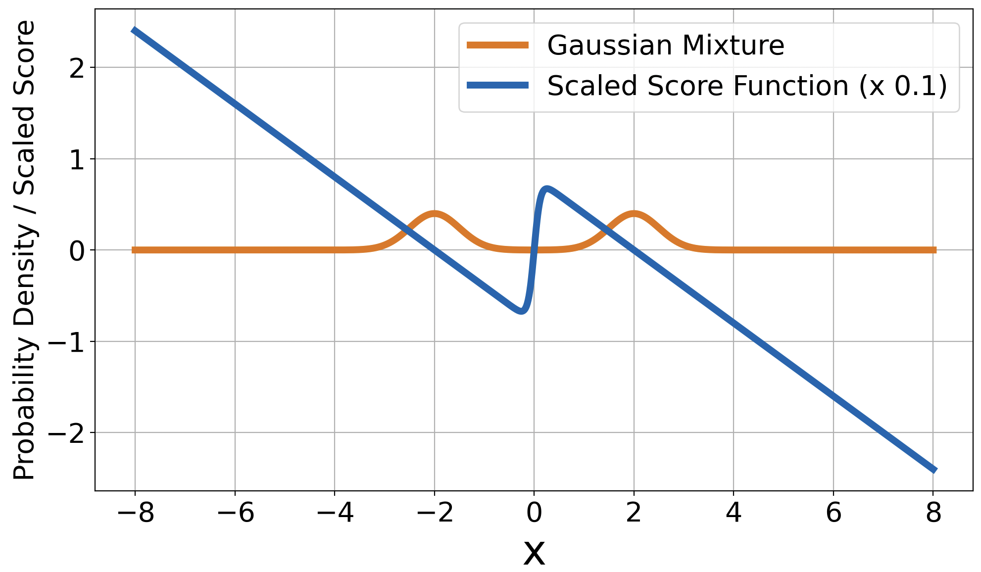
see Appendix A.3.1 for value of b0superscriptsubscript𝑏0b_{0}^{\star}. Note the optimal score is a piecewise linear function with breakpoints only at a subset of data points. When training data points are highly separated, the optimal score approximately corresponds to score of mixture of Gaussian with centroids at {x~:y~(x~)=0}conditional-set~𝑥~𝑦~𝑥0\{\tilde{x}:\tilde{y}(\tilde{x})=0\}. Moreover, the breakpoints correspond to the extreme points in each Gaussian component. See Figure 6 in Appendix A.3.1 for score functions for single Gaussian distribution and Gaussian mixture distribution with separated centroids.

3.2.2 Multivariate Data

To state the convex program for multivariate data, we first introduce the concept of arrangement matrices. When d𝑑d is arbitrary, for data matrix Xn×d𝑋superscript𝑛𝑑X\in\mathbb{R}^{n\times d} and any arbitrary vector ud𝑢superscript𝑑u\in\mathbb{R}^{d}, We consider the set of diagonal matrices

𝒟:={diag(𝟙{Xu0})},assign𝒟diag1𝑋𝑢0\mathcal{D}:=\{\text{diag}({\mathbbm{1}}\{Xu\geq 0\})\},

which takes value 111 or 00 along the diagonal that indicates the set of possible arrangement activation patterns for the ReLU activation. Indeed, we can enumerate the set of sign patterns as 𝒟={Di}i=1P𝒟superscriptsubscriptsubscript𝐷𝑖𝑖1𝑃\mathcal{D}=\{D_{i}\}_{i=1}^{P} where P𝑃P is bounded by

P2r(e(n1)r)r𝑃2𝑟superscript𝑒𝑛1𝑟𝑟P\leq 2r\left(\frac{e(n-1)}{r}\right)^{r}

for r=rank(X)𝑟rank𝑋r=\text{rank}(X) (Pilanci & Ergen, 2020; Stanley et al., 2004). Now we are ready to present the convex program for multivariate data below. Since the proof of Theorem 3.1 is closely tied to reconstruction of optimal neurons and does not trivially extend to multivariate data, we instead follow (Mishkin et al., 2022) and employ an alternative duality-free proof for Theorem 3.2 to derive

Theorem 3.2.

When σ𝜎\sigma is ReLU, V=0𝑉0V=0 and β=0,𝛽0\beta=0, denote the optimal score matching objective value (2) with sθsubscript𝑠𝜃s_{\theta} specified in (3) as psuperscript𝑝p^{*}, when m2Pd𝑚2𝑃𝑑m\geq 2Pd, under Assumption A.8,

p=minWi12i=1PDiXWiF2+i=1Ptr(Di)tr(Wi),superscript𝑝subscriptsubscript𝑊𝑖12superscriptsubscriptnormsuperscriptsubscript𝑖1𝑃subscript𝐷𝑖𝑋subscript𝑊𝑖𝐹2superscriptsubscript𝑖1𝑃trsubscript𝐷𝑖trsubscript𝑊𝑖p^{*}=\min_{W_{i}}\frac{1}{2}\left\|\sum_{i=1}^{P}D_{i}XW_{i}\right\|_{F}^{2}+\sum_{i=1}^{P}\text{tr}(D_{i})\text{tr}(W_{i}), (5)

where Wid×dsubscript𝑊𝑖superscript𝑑𝑑W_{i}\in\mathbb{R}^{d\times d}.

Proof.

See Appendix A.9.1. ∎

See Appendix A.9 for convex program for more model types. Denote V~=[tr(D1)I,tr(D2)I,,tr(DP)I],W=[W1,,WP]T,X~=[D1X,,DPX]formulae-sequence~𝑉trsubscript𝐷1𝐼trsubscript𝐷2𝐼trsubscript𝐷𝑃𝐼formulae-sequence𝑊superscriptsubscript𝑊1subscript𝑊𝑃𝑇~𝑋subscript𝐷1𝑋subscript𝐷𝑃𝑋\tilde{V}=[\mbox{tr}(D_{1})I,\mbox{tr}(D_{2})I,\ldots,\mbox{tr}(D_{P})I],W=[W_{1},\ldots,W_{P}]^{T},\tilde{X}=[D_{1}X,\ldots,D_{P}X], then the convex program (5) can be rewritten as

minW12X~WF2+V~,W.subscript𝑊12superscriptsubscriptnorm~𝑋𝑊𝐹2~𝑉𝑊\min_{W}\frac{1}{2}\big{\|}\tilde{X}W\big{\|}_{F}^{2}+\langle\tilde{V},W\rangle. (6)

When the optimal value is finite, e.g., V~range(X~TX~)~𝑉rangesuperscript~𝑋𝑇~𝑋\tilde{V}\in\mathrm{range}(\tilde{X}^{T}\tilde{X}), an optimal solution to (6) is given by

W𝑊\displaystyle W =(X~TX~)V~absentsuperscriptsuperscript~𝑋𝑇~𝑋~𝑉\displaystyle=(\tilde{X}^{T}\tilde{X})^{\dagger}\tilde{V}
=[kS11XkXkTkS12XkXkTkS21XkXkTkS22XkXkT][tr(D1)Itr(D2)Itr(DP)I],absentsuperscriptmatrixsubscript𝑘subscript𝑆11subscript𝑋𝑘superscriptsubscript𝑋𝑘𝑇subscript𝑘subscript𝑆12subscript𝑋𝑘superscriptsubscript𝑋𝑘𝑇subscript𝑘subscript𝑆21subscript𝑋𝑘superscriptsubscript𝑋𝑘𝑇subscript𝑘subscript𝑆22subscript𝑋𝑘superscriptsubscript𝑋𝑘𝑇missing-subexpressionmissing-subexpressionmatrixtrsubscript𝐷1𝐼trsubscript𝐷2𝐼trsubscript𝐷𝑃𝐼\displaystyle=\begin{bmatrix}\sum_{k\in S_{11}}X_{k}X_{k}^{T}&\sum_{k\in S_{12}}X_{k}X_{k}^{T}&\cdots\\ \sum_{k\in S_{21}}X_{k}X_{k}^{T}&\sum_{k\in S_{22}}X_{k}X_{k}^{T}&\cdots\\ &\cdots&\end{bmatrix}^{\dagger}\begin{bmatrix}\mbox{tr}(D_{1})I\\ \mbox{tr}(D_{2})I\\ \vdots\\ \mbox{tr}(D_{P})I\end{bmatrix},

where Sij={k:XkTui0,XkTuj0}subscript𝑆𝑖𝑗conditional-set𝑘formulae-sequencesuperscriptsubscript𝑋𝑘𝑇subscript𝑢𝑖0superscriptsubscript𝑋𝑘𝑇subscript𝑢𝑗0S_{ij}=\{k:X_{k}^{T}u_{i}\geq 0,X_{k}^{T}u_{j}\geq 0\} and uisubscript𝑢𝑖u_{i} is the generator of Di=diag(𝟙{Xui0})subscript𝐷𝑖diag1𝑋subscript𝑢𝑖0D_{i}=\text{diag}({\mathbbm{1}}\{Xu_{i}\geq 0\}).

Remark 3.3.

Note that the above model can be seen as a piecewise empirical covariance estimator which partitions the space with hyperplane arrangements. When P=1𝑃1P=1, D1=Isubscript𝐷1𝐼D_{1}=I and XTXsuperscript𝑋𝑇𝑋X^{T}X is invertible, then (X~TX~)superscriptsuperscript~𝑋𝑇~𝑋(\tilde{X}^{T}\tilde{X})^{\dagger} reduces to the empirical precision matrix which models the correlation between different data points. This was observed in the application of score matching objective in graphical models (Hyvärinen, 2005; Lin et al., 2016) with NNs with linear activation. Here, we obtain a more expressive model with non-linear neural network through data partitioning.

3.3 Special Case: Large Weight Decay Regime

In this section, we investigate convex program (4) assuming training data x1,,xnsubscript𝑥1subscript𝑥𝑛x_{1},\ldots,x_{n}\in\mathbb{R} are distinct. We show that for large β𝛽\beta, program (4) can be solved analytically and the integration of predicted score function is always concave for ReLU activation, which aligns with theoretic assumptions for log-concave sampling procedures. Note this does not happen for absolute value activation, where the predicted score function may integrate to be non-concave and only convergence to stationary points holds in this regime.

Consider convex program (4). For NNs with ReLU activation and without skip connection, An×4n𝐴superscript𝑛4𝑛A\in\mathbb{R}^{n\times 4n} and y4n𝑦superscript4𝑛y\in\mathbb{R}^{4n}. When β>b,y=0formulae-sequence𝛽subscriptnorm𝑏𝑦0\beta>\|b\|_{\infty},y=0 is optimal and the neural network will always output zero. When β1<βbsubscript𝛽1𝛽subscriptnorm𝑏\beta_{1}<\beta\leq\|b\|_{\infty} for some threshold β1subscript𝛽1\beta_{1}222See Appendix A.5 for value of β1subscript𝛽1\beta_{1}., y𝑦y is all zero except for the first and the 3n3𝑛3n-th entry, which have value (βn)/2nv+t𝛽𝑛2𝑛𝑣𝑡(\beta-n)/2nv+t and (nβ)/2nv+t𝑛𝛽2𝑛𝑣𝑡(n-\beta)/2nv+t for any |t|nβ2nv𝑡𝑛𝛽2𝑛𝑣|t|\leq\frac{n-\beta}{2nv} correspondingly, see Appendix A.5 for proof. For any input data point x^,^𝑥\hat{x}, the predicted score y^^𝑦\hat{y} is

{y^=βnnv(x^μ),x1x^xny^=(nβ2nv+t)x^+(βn2nv+t)x1+nβnvμ,x^<x1y^=(βn2nv+t)x^(nβ2nv+t)xn+nβnvμ,x^>xncasesformulae-sequence^𝑦𝛽𝑛𝑛𝑣^𝑥𝜇subscript𝑥1^𝑥subscript𝑥𝑛otherwiseformulae-sequence^𝑦𝑛𝛽2𝑛𝑣𝑡^𝑥𝛽𝑛2𝑛𝑣𝑡subscript𝑥1𝑛𝛽𝑛𝑣𝜇^𝑥subscript𝑥1otherwiseformulae-sequence^𝑦𝛽𝑛2𝑛𝑣𝑡^𝑥𝑛𝛽2𝑛𝑣𝑡subscript𝑥𝑛𝑛𝛽𝑛𝑣𝜇^𝑥subscript𝑥𝑛otherwise\begin{cases}\hat{y}=\frac{\beta-n}{nv}(\hat{x}-\mu),~{}~{}\qquad\qquad\qquad\qquad\quad x_{1}\leq\hat{x}\leq x_{n}\\ \hat{y}=-(\frac{n-\beta}{2nv}+t)\hat{x}+(\frac{\beta-n}{2nv}+t)x_{1}+\frac{n-\beta}{nv}\mu,~{}\quad\hat{x}<x_{1}\\ \hat{y}=(\frac{\beta-n}{2nv}+t)\hat{x}-(\frac{n-\beta}{2nv}+t)x_{n}+\frac{n-\beta}{nv}\mu,\qquad\hat{x}>x_{n}\end{cases} (7)

for some |t|nβ2nv𝑡𝑛𝛽2𝑛𝑣|t|\leq\frac{n-\beta}{2nv}, where μ=i=1nxi/n𝜇superscriptsubscript𝑖1𝑛subscript𝑥𝑖𝑛\mu=\sum_{i=1}^{n}x_{i}/n denotes the sample mean and v=i=1n(xiμ)2/n𝑣superscriptsubscript𝑖1𝑛superscriptsubscript𝑥𝑖𝜇2𝑛v=\sum_{i=1}^{n}(x_{i}-\mu)^{2}/n denotes the sample variance.

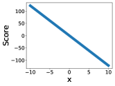
Figure 1: Predicted score function (left) and its integration (right) for univariate data for two-layer ReLU neural network. The left plot shows all optimal score predictions by convex score predictor for weight decay parameter β1<βnsubscript𝛽1𝛽𝑛{\color[rgb]{0,0,0}\definecolor[named]{pgfstrokecolor}{rgb}{0,0,0}\pgfsys@color@gray@stroke{0}\pgfsys@color@gray@fill{0}\beta_{1}}<\beta\leq n and for univariate input data of arbitrary distribution. See Section 3.3 for details.

Figure 1 shows the score function prediction of (7) and its integration. Note within sampled data range, the predicted score function aligns with score function of Gaussian distribution parameterized by sample mean μ𝜇\mu and sample variance v𝑣v; outside data range, the predicted score function is a linear interpolation. The integration of score function is always concave in this case, and therefore Langevin dynamics sampling with predicted score function has well-established convergence guarantees (Durmus & Moulines, 2016a; Dalalyan, 2016; Durmus & Moulines, 2016b). Here we make a comparison with the predicted score for neural network with absolute value activation without skip connection, when β𝛽\beta goes below n𝑛n (see Appendix A.6.1 for details), for any test data x^^𝑥\hat{x}, the corresponding predicted score y^^𝑦\hat{y} is given by

{y^=βnnv(x^μ),x1x^xn,y^=2tx^+(βnnv+2t)x1+nβnvμ,x^<x1,y^=2tx^(nβnv+2t)xn+nβnvμ,x^>xn.cases^𝑦𝛽𝑛𝑛𝑣^𝑥𝜇subscript𝑥1^𝑥subscript𝑥𝑛^𝑦2𝑡^𝑥𝛽𝑛𝑛𝑣2𝑡subscript𝑥1𝑛𝛽𝑛𝑣𝜇^𝑥subscript𝑥1^𝑦2𝑡^𝑥𝑛𝛽𝑛𝑣2𝑡subscript𝑥𝑛𝑛𝛽𝑛𝑣𝜇^𝑥subscript𝑥𝑛\begin{cases}\hat{y}=\frac{\beta-n}{nv}(\hat{x}-\mu),\quad&x_{1}\leq\hat{x}\leq x_{n},\\ \hat{y}=-2t\hat{x}+(\frac{\beta-n}{nv}+2t)x_{1}+\frac{n-\beta}{nv}\mu,\quad&\hat{x}<x_{1},\\ \hat{y}=2t\hat{x}-(\frac{n-\beta}{nv}+2t)x_{n}+\frac{n-\beta}{nv}\mu,\quad&\hat{x}>x_{n}.\end{cases}
Figure 2: Predicted score function (left) and its integration (right) for univariate data for two-layer absolute value activation neural network. The left plot shows all optimal score predictions by convex score predictor for weight decay parameter β2<βnsubscript𝛽2𝛽𝑛{\color[rgb]{0,0,0}\definecolor[named]{pgfstrokecolor}{rgb}{0,0,0}\pgfsys@color@gray@stroke{0}\pgfsys@color@gray@fill{0}\beta_{2}}<\beta\leq n and for univariate input data of arbitrary distribution. See Section 3.3 for details.

Figure 2 depicts the score prediction and its integration. Within the sampled data range, the score prediction corresponds to score of Gaussian distribution parameterized by sample mean and sample variance which is the same as the score predicted by ReLU neural network. The score prediction outside sampled data range is a linear interpolation with a different slope from what is predicted by the ReLU neural network. This underscores the distinction between absolute value activation and ReLU activation. The corresponding probability density is log-concave only when t=0𝑡0t=0. Notably, the solution with t=0𝑡0t=0 corresponds to the unique minimum norm solution of the convex program (4), highlighting its significance. Here the score prediction no longer corresponds to log-concave distribution except for the min-norm case and classic convergence theory has only theoretic assurance for converging to stationary points (Chewi, 2023). When it comes to difference between neural networks with and without skip connection, for large β>n𝛽𝑛\beta>n, the optimal score prediction is all zeros for NNs without skip connection. When skip connection is added, the optimal score prediction is no longer zero and the corresponding neural network parameter set is given by {W(1)=0,b(1)=0,W(2)=0,b(2)=μ/v,V=1/v}formulae-sequencesuperscript𝑊10formulae-sequencesuperscript𝑏10formulae-sequencesuperscript𝑊20formulae-sequencesuperscript𝑏2𝜇𝑣𝑉1𝑣\{W^{(1)}=0,b^{(1)}=0,W^{(2)}=0,b^{(2)}=\mu/v,V=-1/v\}. For any test data x^^𝑥\hat{x}, the corresponding predicted score is given by

y^=Vx^+b(2)=1v(x^μ),^𝑦𝑉^𝑥superscript𝑏21𝑣^𝑥𝜇\hat{y}=V\hat{x}+b^{(2)}=-\frac{1}{v}(\hat{x}-\mu),

which gives the score function of Gaussian distribution with mean being sample mean and variance being sample variance.Therefore, adding skip connection would change the zero score prediction to a linear function parameterized by sample mean and variance in the large weight decay regime. See Appendix A.6.2 and A.6.3 for details.

3.4 Convergence Result

Consider two-layer ReLU network without skip connection and training points x1,,xnsubscript𝑥1subscript𝑥𝑛x_{1},\ldots,x_{n}\in\mathbb{R}. For neural network-based score function predictor, note once y4nsuperscript𝑦superscript4𝑛y^{\star}\in\mathbb{R}^{4n} to the convex program (4) is known, for any input data x𝑥x, the score prediction is given by

s(x)=i=1nyiT𝒟(x,xi)+b0,𝑠𝑥superscriptsubscript𝑖1𝑛superscriptsuperscriptsubscriptsuperscript𝑦𝑖𝑇𝒟𝑥subscript𝑥𝑖superscriptsubscript𝑏0s(x)=\sum_{i=1}^{n}{{y^{\prime}_{i}}^{\star}}^{T}\mathcal{D}(x,x_{i})+b_{0}^{\star},

where yi4superscriptsuperscriptsubscript𝑦𝑖superscript4{y_{i}^{\prime}}^{\star}\in\mathbb{R}^{4} is constant expressed in y,𝒟(x,xi)4superscript𝑦𝒟𝑥subscript𝑥𝑖superscript4y^{\star},\mathcal{D}(x,x_{i})\in\mathbb{R}^{4} is entrywise piecewise linear with kinks at xi.subscript𝑥𝑖x_{i}. b0superscriptsubscript𝑏0b_{0}^{\star} is constant. See Appendix A.8 for definition of yi,𝒟()superscriptsuperscriptsubscript𝑦𝑖𝒟{y_{i}^{\prime}}^{\star},\mathcal{D}(\cdot) and b0superscriptsubscript𝑏0b_{0}^{\star}. Integrating the above score function we get

s(x)𝑑x=12i=1nyiT𝒟2(x,xi)+b0x.𝑠𝑥differential-d𝑥12superscriptsubscript𝑖1𝑛superscriptsuperscriptsubscriptsuperscript𝑦𝑖𝑇superscript𝒟2𝑥subscript𝑥𝑖superscriptsubscript𝑏0𝑥\int s(x)dx=\frac{1}{2}\sum_{i=1}^{n}{{y^{\prime}_{i}}^{\star}}^{T}\mathcal{D}^{2}(x,x_{i})+b_{0}^{\star}x.

The corresponding probability density is proportional to

exp(s(x)𝑑x)=exp(12i=1nyiT𝒟2(x,xi)+b0x).𝑠𝑥differential-d𝑥12superscriptsubscript𝑖1𝑛superscriptsuperscriptsubscriptsuperscript𝑦𝑖𝑇superscript𝒟2𝑥subscript𝑥𝑖superscriptsubscript𝑏0𝑥\exp(\int s(x)dx)=\exp(\frac{1}{2}\sum_{i=1}^{n}{{y^{\prime}_{i}}^{\star}}^{T}\mathcal{D}^{2}(x,x_{i})+b_{0}^{\star}x).

Note that the log-density is piecewise quadratic with breakpoints only at a subset of training points.

Strong convergence guarantees for Langevin Monte Carlo method are often contingent upon the log-concavity of the target distribution. Notably, in Section 3.3 we analyze the predicted score function in certain ranges of weight decay. These score functions correspond to log concave distributions for ReLU activation and thus we can exploit existing convergence results for Langevin dynamics to derive the convergence of diffusion model with a neural network-based score function. Here, we follow notations used in Section 3.3. Algorithms of score matching and Langevin sampling are given in Algorithm 1 and 2 respectively. To the best of our knowledge, prior to our study, there has been no characterization of the sample distribution generated by Algorithm 2 when the score model is trained using Algorithm 1.

Algorithm 1 Score Matching
  Input: training data x1,,xndsubscript𝑥1subscript𝑥𝑛superscript𝑑x_{1},\ldots,x_{n}\in\mathbb{R}^{d}
  minimize
i=1n12sθ2(xi)+θsθ(xi)+β2θ22superscriptsubscript𝑖1𝑛12superscriptsubscript𝑠𝜃2subscript𝑥𝑖subscript𝜃subscript𝑠𝜃subscript𝑥𝑖𝛽2superscriptsubscriptnormsuperscript𝜃22\sum_{i=1}^{n}\frac{1}{2}s_{\theta}^{2}(x_{i})+\nabla_{\theta}s_{\theta}(x_{i})+\frac{\beta}{2}\|\theta^{\prime}\|_{2}^{2}
Theorem 3.4.

When sθsubscript𝑠𝜃s_{\theta} is of two-layer ReLU and β1<βn,subscript𝛽1𝛽𝑛{\color[rgb]{0,0,0}\definecolor[named]{pgfstrokecolor}{rgb}{0,0,0}\pgfsys@color@gray@stroke{0}\pgfsys@color@gray@fill{0}\beta_{1}}<\beta\leq n,333See Section 3.3 for value of β1subscript𝛽1\beta_{1} let π𝜋\pi denote the target distribution (defined below). For any ϵ[0,1]italic-ϵ01\epsilon\in[0,1], if we take step size ηϵ2nvnβ,asymptotically-equals𝜂superscriptitalic-ϵ2𝑛𝑣𝑛𝛽\eta\asymp\frac{\epsilon^{2}nv}{n-\beta}, then for the mixture distribution μ¯=T1t=1Txt¯𝜇superscript𝑇1superscriptsubscript𝑡1𝑇superscript𝑥𝑡\overline{\mu}=T^{-1}\sum_{t=1}^{T}x^{t}, it holds that KL(μ¯π)ϵKLconditional¯𝜇𝜋italic-ϵ\sqrt{\text{KL}(\overline{\mu}\|\pi)}\leq\epsilon after

O((nβ)W22(μ0,π)nvϵ4)iterations,𝑂𝑛𝛽superscriptsubscript𝑊22subscript𝜇0𝜋𝑛𝑣superscriptitalic-ϵ4iterationsO\left(\frac{(n-\beta)W_{2}^{2}(\mu_{0},\pi)}{nv\epsilon^{4}}\right)\quad\text{iterations},

where W2subscript𝑊2W_{2} denotes 2-Wasserstein distance and π𝜋\pi satisfies

π{exp((βn4nvt2)x2+(βn2nv+t)x1x+(μ(nβ)nv)x+(nβ4nvt2)x12),x<x1,exp(βn2nvx2μ(βn)nvx),x1xxn,exp((βn4nv+t2)x2(nβ2nv+t)xnx+(μ(nβ)nv)x+(t2+nβ4nv)xn2),xxn,\pi\propto\begin{cases}\exp((\frac{\beta-n}{4nv}-\frac{t}{2})x^{2}+(\frac{\beta-n}{2nv}+t)x_{1}x\\ \qquad+(\frac{\mu(n-\beta)}{nv})x+(\frac{n-\beta}{4nv}-\frac{t}{2})x_{1}^{2}),\qquad x<x_{1},\\ \exp(\frac{\beta-n}{2nv}x^{2}-\frac{\mu(\beta-n)}{nv}x),\qquad\qquad x_{1}\leq x\leq x_{n},\\ \exp((\frac{\beta-n}{4nv}+\frac{t}{2})x^{2}-(\frac{n-\beta}{2nv}+t)x_{n}x\\ \qquad+(\frac{\mu(n-\beta)}{nv})x+(\frac{t}{2}+\frac{n-\beta}{4nv})x_{n}^{2}),\qquad x\geq x_{n},\end{cases}

for some |t|nβ2nv𝑡𝑛𝛽2𝑛𝑣|t|\leq\frac{n-\beta}{2nv}.

Proof.

See Appendix A.8. ∎

Theorem 3.4 is a simple extension of prior literature for log-concave sampling convergence given we derive the NN-predicted score and the distribution it characterizes is indeed log-concave.

Algorithm 2 Langevin Monte Carlo
  Initialize: x0μ0(x)similar-tosuperscript𝑥0subscript𝜇0𝑥x^{0}\sim\mu_{0}(x)
  for t=1,2,,T𝑡12𝑇t=1,2,...,T do
     zt𝒩(0,1)similar-tosuperscript𝑧𝑡𝒩01z^{t}\sim\mathcal{N}(0,1)
     xtxt1+ϵ2sθ(xt1)+ϵztsuperscript𝑥𝑡superscript𝑥𝑡1italic-ϵ2subscript𝑠𝜃superscript𝑥𝑡1italic-ϵsuperscript𝑧𝑡x^{t}\leftarrow x^{t-1}+\frac{\epsilon}{2}s_{\theta}(x^{t-1})+\sqrt{\epsilon}z^{t}
  end for

4 Denoising Score Matching Objective

To tackle the difficulty in computation of trace of Jacobian required in score matching objective (1), denoising score matching has been proposed in (Vincent, 2011). It then becomes widely used in practical generative models. In this section, we derive convex programs for the denoising score matching objective.

To briefly introduce, denoising score matching first perturbs data points with a predefined noise distribution and then estimates the score of the perturbed data distribution. When the noise distribution is chosen to be standard Gaussian, for some noise level ϵ>0italic-ϵ0\epsilon>0, the objective is equivalent to

minθ𝔼xp(x)𝔼δ𝒩(0,I)sθ(x+ϵδ)δϵ22,subscript𝜃subscript𝔼similar-to𝑥𝑝𝑥subscript𝔼similar-to𝛿𝒩0𝐼superscriptsubscriptnormsubscript𝑠𝜃𝑥italic-ϵ𝛿𝛿italic-ϵ22\min_{\theta}\mathbb{E}_{x\sim p(x)}\mathbb{E}_{\delta\sim\mathcal{N}(0,I)}\left\|s_{\theta}(x+\epsilon\delta)-\frac{\delta}{\epsilon}\right\|_{2}^{2},

and the empirical version is given by

𝐃𝐒𝐌(sθ)=i=1n12sθ(xi+ϵδi)δiϵ22,𝐃𝐒𝐌subscript𝑠𝜃superscriptsubscript𝑖1𝑛12superscriptsubscriptnormsubscript𝑠𝜃subscript𝑥𝑖italic-ϵsubscript𝛿𝑖subscript𝛿𝑖italic-ϵ22\mathbf{DSM}(s_{\theta})=\sum_{i=1}^{n}\frac{1}{2}\left\|s_{\theta}(x_{i}+\epsilon\delta_{i})-\frac{\delta_{i}}{\epsilon}\right\|_{2}^{2}, (8)

where {xi}i=1nsuperscriptsubscriptsubscript𝑥𝑖𝑖1𝑛\{x_{i}\}_{i=1}^{n} are samples from p(x)𝑝𝑥p(x) and {δi}i=1nsuperscriptsubscriptsubscript𝛿𝑖𝑖1𝑛\{\delta_{i}\}_{i=1}^{n} are samples from standard Gaussian. The final training loss we consider is the above score matching objective together with weight decay term, which writes

minθ𝐃𝐒𝐌(sθ(x))+β2θ22,subscript𝜃𝐃𝐒𝐌subscript𝑠𝜃𝑥𝛽2superscriptsubscriptnormsuperscript𝜃22\min_{\theta}\mathbf{DSM}(s_{\theta}(x))+\frac{\beta}{2}\|\theta^{\prime}\|_{2}^{2}, (9)

where θθsuperscript𝜃𝜃\theta^{\prime}\subseteq\theta denotes the parameters to be regularized. Unlike for score matching objective where weight decay is important for optimal objective value to stay finite, here for denoising objective, weight decay is unnecessary and can be removed. In our derived convex program, we allow β𝛽\beta to be arbitrarily close to zero so the result is general. Note (9) circumvents the computation of trace of Jacobian and is thus more applicable for training tasks in large data regime. One drawback is that optimal sθsubscript𝑠𝜃s_{\theta} that minimizes (9) measures score function of the perturbed data and is only close to original data distribution when noise is small enough. We consider the same neural network architecture described in Section 3.1.

4.1 Univariate Data

We follow similar analysis pattern as in Section 3 and consider univariate data first. The following theorem states the convex program for denoising score matching objective (9) for univariate data with two-layer ReLU neural network. See Appendix B.2 for convex programs for more model architectures.

Theorem 4.1.

When σ𝜎\sigma is ReLU and V=0𝑉0V=0, denote the optimal denoising score matching objective value (9) with sθsubscript𝑠𝜃s_{\theta} specified in (3) as p,superscript𝑝p^{*}, when β>0𝛽0\beta>0 and mm𝑚superscript𝑚m\geq m^{\ast},

p=superscript𝑝absent\displaystyle p^{*}= miny12Ay+b22+βy1,subscript𝑦12superscriptsubscriptnorm𝐴𝑦𝑏22𝛽subscriptnorm𝑦1\displaystyle\min_{y}\quad\frac{1}{2}\|Ay+b\|_{2}^{2}+\beta\|y\|_{1}\,, (10)

where m=y0superscript𝑚subscriptnormsuperscript𝑦0m^{*}=\|y^{*}\|_{0}, and ysuperscript𝑦y^{*} is any optimal solution to (10). A,b𝐴𝑏A,b is specified in Appendix B.1.

Proof.

See Appendix B.1. ∎

Once an optimal ysuperscript𝑦y^{\star} of convex program (10) has been obtained, the optimal score prediction for any input x𝑥x is given by

sθ(x)=i=1nyi(xxi)+i=1nyn+i(x+xi)+b0,subscript𝑠superscript𝜃𝑥superscriptsubscript𝑖1𝑛superscriptsubscript𝑦𝑖subscript𝑥subscript𝑥𝑖superscriptsubscript𝑖1𝑛superscriptsubscript𝑦𝑛𝑖subscript𝑥subscript𝑥𝑖superscriptsubscript𝑏0s_{\theta^{\star}}(x)=-\sum_{i=1}^{n}y_{i}^{\star}(x-x_{i})_{+}-\sum_{i=1}^{n}y_{n+i}^{\star}(-x+x_{i})_{+}b_{0}^{\star},

with b0=1n1T([A1,A2]y+l)superscriptsubscript𝑏01𝑛superscript1𝑇subscript𝐴1subscript𝐴2superscript𝑦𝑙{\color[rgb]{0,0,0}\definecolor[named]{pgfstrokecolor}{rgb}{0,0,0}\pgfsys@color@gray@stroke{0}\pgfsys@color@gray@fill{0}b_{0}^{\star}}=\frac{1}{n}1^{T}([A_{1},A_{2}]y^{\star}+l) where [A1]ij=(xixj)+subscriptdelimited-[]subscript𝐴1𝑖𝑗subscriptsubscript𝑥𝑖subscript𝑥𝑗[A_{1}]_{ij}=(x_{i}-x_{j})_{+} and [A2]ij=(xi+xj)+subscriptdelimited-[]subscript𝐴2𝑖𝑗subscriptsubscript𝑥𝑖subscript𝑥𝑗[A_{2}]_{ij}=(-x_{i}+x_{j})_{+}. l𝑙l is the label vector, i.e, l=[δ1/ϵ,δ2/ϵ,,δn/ϵ]T𝑙superscriptsubscript𝛿1italic-ϵsubscript𝛿2italic-ϵsubscript𝛿𝑛italic-ϵ𝑇l=[\delta_{1}/\epsilon,\delta_{2}/\epsilon,\ldots,\delta_{n}/\epsilon]^{T}.

4.2 Multivariate Data

Now we consider multivariate data regime. The below theorem gives the convex program equivalent to the denoising score matching objective (9) for multivariate data. Let Ln×d𝐿superscript𝑛𝑑L\in\mathbb{R}^{n\times d} denote the label matrix, i.e., Li=δi/ϵsubscript𝐿𝑖subscript𝛿𝑖italic-ϵL_{i}=\delta_{i}/\epsilon, and 𝒟={Di}i=1P𝒟superscriptsubscriptsubscript𝐷𝑖𝑖1𝑃\mathcal{D}=\{D_{i}\}_{i=1}^{P} be the arrangement activation patterns for ReLU activation as defined in Section 3.2.2. See Appendix B.3 for convex programs for more model types.

Theorem 4.2.

When σ𝜎\sigma is ReLU, V=0𝑉0V=0 and β=0𝛽0\beta=0, denote the optimal denoising score matching objective value (9) with sθsubscript𝑠𝜃s_{\theta} specified in (3) as psuperscript𝑝p^{*}, when m2Pd𝑚2𝑃𝑑m\geq 2Pd, under Assumption A.8,

p=minWi12i=1PDiXWiLF2,superscript𝑝subscriptsubscript𝑊𝑖12superscriptsubscriptnormsuperscriptsubscript𝑖1𝑃subscript𝐷𝑖𝑋subscript𝑊𝑖𝐿𝐹2p^{*}=\min_{W_{i}}\frac{1}{2}\left\|\sum_{i=1}^{P}D_{i}XW_{i}-L\right\|_{F}^{2}, (11)

where Wid×dsubscript𝑊𝑖superscript𝑑𝑑W_{i}\in\mathbb{R}^{d\times d}.

Proof.

see Appendix B.3.

Note the derived convex program (11) is a simple quadratic program and any convex program solver can be used to solve it efficiently.

5 Numerical Results

We present score matching objective simulation results in Section 5.1 and denoising score matching objective simulation in Section 5.2, see Appendix C for additional simulations for different model types and for uniformly distributed training data.

5.1 Score Matching Objective

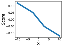
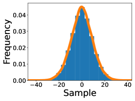
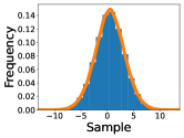
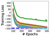
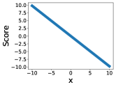
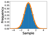
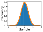
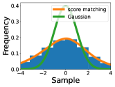
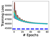
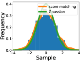
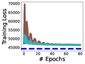
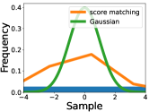
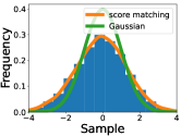
For univariate data and two-layer neural network with ReLU activation considered in Section 3.2.1, Figure 3 shows our simulation results for score matching tasks. We take n=500𝑛500n=500 data points sampled from standard Gaussian and we take weight decay parameter β=b1𝛽subscriptnorm𝑏1\beta=\|b\|_{\infty}-1.444See Section 3.2.1 for definition of b𝑏b. The left plot in Figure 3 shows the training loss where the dashed blue line is the objective value obtained by convex score predictor (4). We solve the convex program analytically as analyzed in Section 3.3 and plot the optimal value. For non-convex neural network training, we run 10 trials with random parameter initiation and use Adam as optimizer with step size 1e21𝑒21e-2. We train for 500 epochs. The result shows that our convex program solves the training problem globally and stably. The middle plot in Figure 3 is the score prediction given by convex neural network, which confirms our derived score function (7). The right plot shows the histogram for running Langevin dynamics sampling in Algorithm 2 with convex score predictor with 105superscript10510^{5} data points and T=500𝑇500T=500 iterations, we take μ0subscript𝜇0\mu_{0} to be uniform distribution from 1010-10 to 101010 and ϵ=1.italic-ϵ1\epsilon=1. Note our convex score predictor recover the ground truth data distribution here.
Refer to caption
Refer to caption
Refer to caption
Figure 3: Simulation results for score matching tasks with two-layer ReLU neural network (Gaussian data). The left plot shows training loss where the dashed blue line indicates loss of convex score predictor (4). The middle plot shows score prediction by convex score predictor, which confirms our analysis in Section 3.3. The right plot shows sampling histogram via Langevin process with convex score predictor.

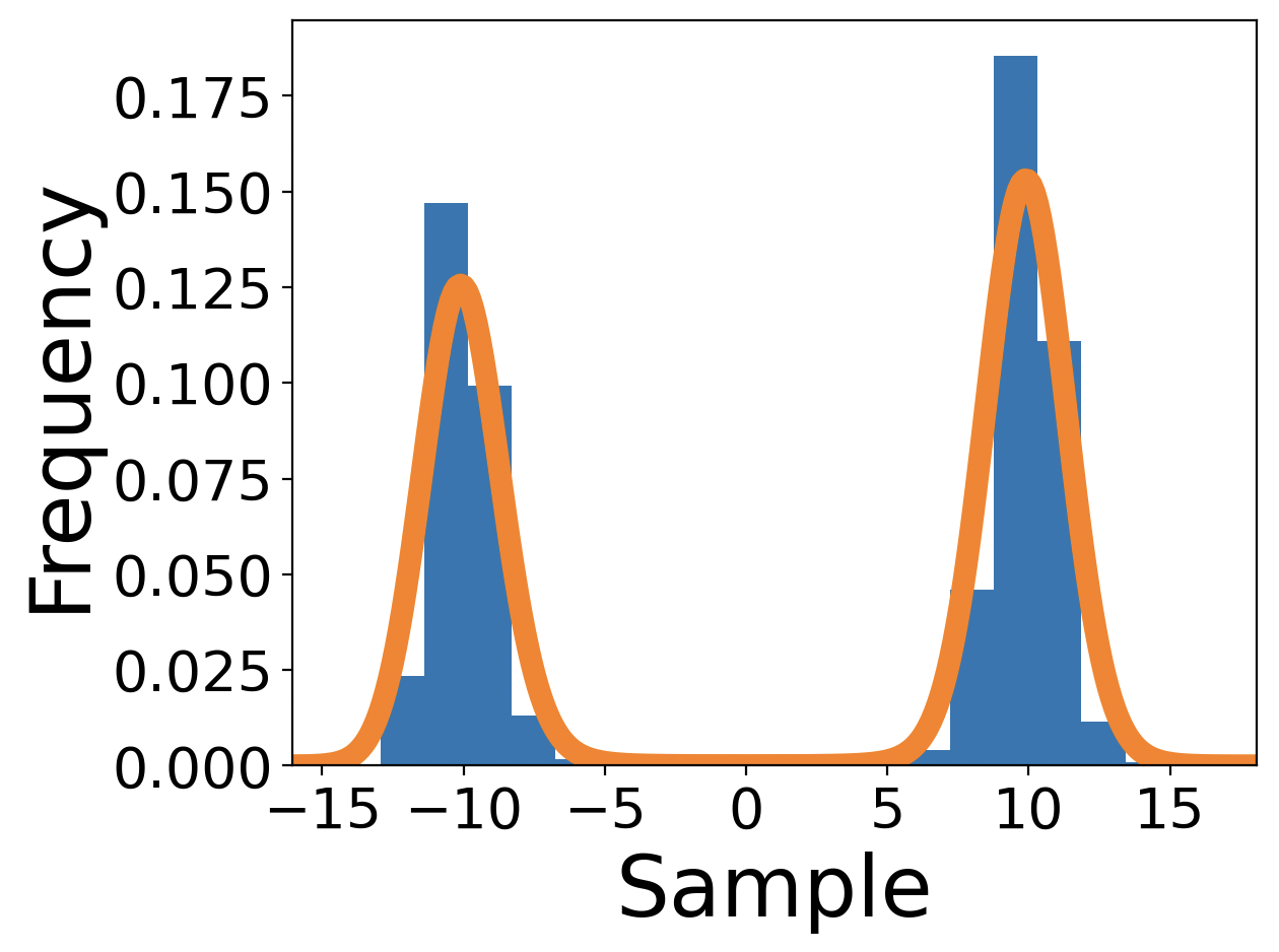
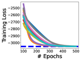
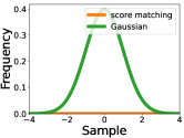
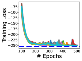
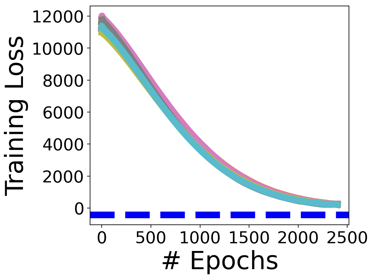
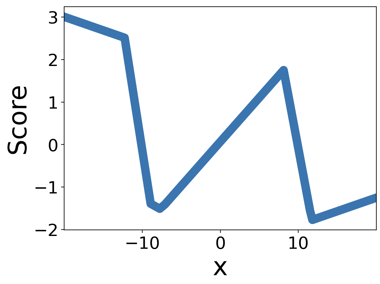
We also test our convex score predictor with Gaussian mixture distribution with two separate centroids. The result is shown in Figure 4. Here we take β=20𝛽20\beta=20 since we know large β𝛽\beta would not generate Gaussian mixture score according to our analysis in Section 3.3. Note our convex score predictor produces the optimal training loss and recovers the ground truth Gaussian mixture distribution.
Refer to caption
Refer to caption
Refer to caption
Figure 4: Simulation results for score matching tasks with two-layer ReLU neural network (Gaussian mixture data). The left plot shows training loss where the dashed blue line indicates loss of convex score predictor (4). The middle plot shows score prediction by convex score predictor. The right plot shows sampling histogram via Langevin process with convex score predictor. The ground truth distribution is Gaussian mixture with two centroids centered at 1010-10 and 101010 respectively and with unit variance, which is recovered by our model.

5.2 Denoising Score Matching Objective

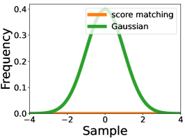
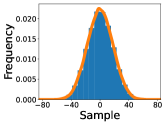
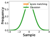
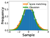
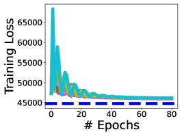
Figure 5 shows our simulation results for denoising score matching tasks. The upper left plot shows denoising score matching training loss where the dashed blue line indicates the loss of convex score predictor from our derived convex program (10) solved with CVXPY. We take weight decay parameter β=0.5𝛽0.5\beta=0.5, n=1000𝑛1000n=1000 data points with standard Gaussian distribution, and noise level ϵ=0.1italic-ϵ0.1\epsilon=0.1 in (8). The non-convex training uses Adam with step size 1e21𝑒21e-2 and takes 200 epochs. We run 10 trials. The notable gap between non-convex training loss and the convex score predictor loss reveals that our convex program solves the training problem globally and stably. The rest plots show the histogram for samples generated via annealed Langevin process (Algorithm 3) with non-convex score predictor and convex score predictor respectively. See Appendix C.2 for experimental hyperparameter choices.

Algorithm 3 Annealed Langevin Sampling
  Initialize: ϵ0,σ1,,σL,x0μ0(x)similar-tosubscriptitalic-ϵ0subscript𝜎1subscript𝜎𝐿superscript𝑥0subscript𝜇0𝑥\epsilon_{0},\sigma_{1},\ldots,\sigma_{L},x^{0}\sim\mu_{0}(x)
  for i=1,2,,L𝑖12𝐿i=1,2,...,L do
     ϵi=ϵ0σi2/σL2subscriptitalic-ϵ𝑖subscriptitalic-ϵ0superscriptsubscript𝜎𝑖2superscriptsubscript𝜎𝐿2\epsilon_{i}=\epsilon_{0}\sigma_{i}^{2}/\sigma_{L}^{2}
     for t=1,2,,T𝑡12𝑇t=1,2,...,T do
        zt𝒩(0,1)similar-tosuperscript𝑧𝑡𝒩01z^{t}\sim\mathcal{N}(0,1)
        xtxt1+ϵi2sθi(xt1)+ϵiztsuperscript𝑥𝑡superscript𝑥𝑡1subscriptitalic-ϵ𝑖2subscript𝑠𝜃𝑖superscript𝑥𝑡1subscriptitalic-ϵ𝑖superscript𝑧𝑡x^{t}\leftarrow x^{t-1}+\frac{\epsilon_{i}}{2}s_{\theta i}(x^{t-1})+\sqrt{\epsilon_{i}}z^{t}
     end for
  end for

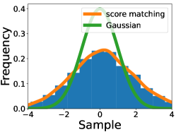
The first histogram shows the generation result with convex score predictor, the third, fourth, and fifth histograms show sampling results with non-convex score predictor corresponding to learning rates 1,1e2,1e611𝑒21𝑒61,1e-2,1e-6 respectively. The first histogram resembles the ground truth Gaussian distribution well while the sampling quality with non-convex score predictor depends heavily on the learning rate choice, which reveal that our convex program is helpful for producing high quality samples stably.
Refer to caption
Refer to caption
Refer to caption
Refer to caption
Refer to caption
Figure 5: Simulation results for denoising score matching tasks with two-layer ReLU neural network. The upper left plot shows training loss where the dashed blue line indicates loss of convex score predictor (10). The second plot shows sampling histogram via annealed Langevin process with convex score predictor. The third, fourth, and fifth plots show sampling histograms via annealed Langevin process with non-convex score predictors trained with learning rates 1,1e2,1e611𝑒21𝑒61,1e-2,1e-6 respectively. The ground truth distribution is standard Gaussian, which is recovered by our model.

6 Conclusion

In this work, we analyze neural network-based diffusion models via lens of convex optimization. We derive an equivalent convex program for two-layer neural networks trained using the score matching objective, which solves the problem globally and bypasses the difficulty of using gradient-based optimizers due to the Jacobian terms. We also derive the convex program for denoising score matching objective. When data is univariate, we find the optimal set of the convex program for the score matching objective for certain weight decay range, and show that for arbitrary data distributions, the neural network-learned score function is piecewise linear and can always be parameterized by sample mean and sample variance. We established convergence results for Langevin sampling with neural network-learned score function.

7 Limitations

In this work, we derive the convex program for score matching objective and denoising score matching objective with weight decay. Though our results hold for general weight decay that can be taken arbitrarily small except for score matching objective where we require reasonable weight decay bound (see Section 3.2.1 for discussion), our convex program always picks the neural network with minimal representation cost. The inductive bias of min-cost NN is not covered in this work. We note that recent work shows stable SGD minimizer has low representation cost (Mulayoff et al., 2021; Nacson et al., 2023). Initializing the weights randomly with small magnitude and running a local optimizer has also been shown to have the same effect as penalizing the weight decay term (Wang & Pilanci, 2021).

Our theory studies shallow two-layer neural network and we leave the extension to deeper NNs as future work. Recent development of convex neural network theory for deeper NNs may provide some insights (Ergen & Pilanci, 2021).

8 Acknowledgements

This work was supported in part by the National Science Foundation (NSF) under Grant DMS-2134248; in part by the NSF CAREER Award under Grant CCF-2236829; in part by the U.S. Army Research Office Early Career Award under Grant W911NF-21-1-0242; in part by the Precourt Institute for Energy and the SystemX Alliance at Stanford University.

References

  • Chewi (2023) Chewi, S. Log-concave sampling, 2023. URL https://chewisinho.github.io/main.pdf.
  • Dalalyan (2016) Dalalyan, A. S. Theoretical guarantees for approximate sampling from smooth and log-concave densities, 2016.
  • Durmus & Moulines (2016a) Durmus, A. and Moulines, É. Sampling from a strongly log-concave distribution with the unadjusted langevin algorithm. arXiv: Statistics Theory, 2016a. URL https://api.semanticscholar.org/CorpusID:124591590.
  • Durmus & Moulines (2016b) Durmus, A. and Moulines, E. Non-asymptotic convergence analysis for the unadjusted langevin algorithm, 2016b.
  • Ergen & Pilanci (2021) Ergen, T. and Pilanci, M. Revealing the structure of deep neural networks via convex duality. In Meila, M. and Zhang, T. (eds.), Proceedings of the 38th International Conference on Machine Learning, volume 139 of Proceedings of Machine Learning Research, pp.  3004–3014. PMLR, 18–24 Jul 2021.
  • Ergen et al. (2023) Ergen, T., Gulluk, H. I., Lacotte, J., and Pilanci, M. Globally optimal training of neural networks with threshold activation functions, 2023.
  • Ho et al. (2020) Ho, J., Jain, A., and Abbeel, P. Denoising diffusion probabilistic models, 2020.
  • Hyvärinen (2005) Hyvärinen, A. Estimation of non-normalized statistical models by score matching. Journal of Machine Learning Research, 6(24):695–709, 2005. URL http://jmlr.org/papers/v6/hyvarinen05a.html.
  • Li et al. (2023) Li, P., Li, Z., Zhang, H., and Bian, J. On the generalization properties of diffusion models, 2023.
  • Lin et al. (2016) Lin, L., Drton, M., and Shojaie, A. Estimation of high-dimensional graphical models using regularized score matching, 2016.
  • Mishkin et al. (2022) Mishkin, A., Sahiner, A., and Pilanci, M. Fast convex optimization for two-layer relu networks: Equivalent model classes and cone decompositions, 2022.
  • Mulayoff et al. (2021) Mulayoff, R., Michaeli, T., and Soudry, D. The implicit bias of minima stability: A view from function space. In Beygelzimer, A., Dauphin, Y., Liang, P., and Vaughan, J. W. (eds.), Advances in Neural Information Processing Systems, 2021. URL https://openreview.net/forum?id=2STmSnZAEt2.
  • Nacson et al. (2023) Nacson, M. S., Mulayoff, R., Ongie, G., Michaeli, T., and Soudry, D. The implicit bias of minima stability in multivariate shallow relu networks, 2023.
  • Pidstrigach (2022) Pidstrigach, J. Score-based generative models detect manifolds, 2022.
  • Pilanci & Ergen (2020) Pilanci, M. and Ergen, T. Neural networks are convex regularizers: Exact polynomial-time convex optimization formulations for two-layer networks, 2020.
  • Sahiner et al. (2021) Sahiner, A., Ergen, T., Pauly, J., and Pilanci, M. Vector-output relu neural network problems are copositive programs: Convex analysis of two layer networks and polynomial-time algorithms, 2021.
  • Sohl-Dickstein et al. (2015) Sohl-Dickstein, J., Weiss, E. A., Maheswaranathan, N., and Ganguli, S. Deep unsupervised learning using nonequilibrium thermodynamics, 2015.
  • Song et al. (2022) Song, J., Meng, C., and Ermon, S. Denoising diffusion implicit models, 2022.
  • Song et al. (2019) Song, Y., Garg, S., Shi, J., and Ermon, S. Sliced score matching: A scalable approach to density and score estimation, 2019.
  • Song et al. (2021) Song, Y., Sohl-Dickstein, J., Kingma, D. P., Kumar, A., Ermon, S., and Poole, B. Score-based generative modeling through stochastic differential equations, 2021.
  • Stanley et al. (2004) Stanley, R. P. et al. An introduction to hyperplane arrangements. Geometric combinatorics, 13(389-496):24, 2004.
  • Vincent (2011) Vincent, P. A connection between score matching and denoising autoencoders. Neural computation, 23(7):1661–1674, 2011.
  • Wang & Pilanci (2021) Wang, Y. and Pilanci, M. The convex geometry of backpropagation: Neural network gradient flows converge to extreme points of the dual convex program, 2021.
  • Wu et al. (2023) Wu, T., Fan, Z., Liu, X., Gong, Y., Shen, Y., Jiao, J., Zheng, H.-T., Li, J., Wei, Z., Guo, J., Duan, N., and Chen, W. Ar-diffusion: Auto-regressive diffusion model for text generation, 2023.
  • Yi et al. (2023) Yi, M., Sun, J., and Li, Z. On the generalization of diffusion model, 2023.
  • Yoon et al. (2023) Yoon, T., Choi, J. Y., Kwon, S., and Ryu, E. K. Diffusion probabilistic models generalize when they fail to memorize. In ICML 2023 Workshop on Structured Probabilistic Inference & Generative Modeling, 2023. URL https://openreview.net/forum?id=shciCbSk9h.
  • Zeno et al. (2023) Zeno, C., Ongie, G., Blumenfeld, Y., Weinberger, N., and Soudry, D. How do minimum-norm shallow denoisers look in function space?, 2023.
  • Zhang et al. (2023) Zhang, C., Zhang, C., Zheng, S., Zhang, M., Qamar, M., Bae, S.-H., and Kweon, I. S. A survey on audio diffusion models: Text to speech synthesis and enhancement in generative ai, 2023.

Appendix A Supplementary Theoretic Materials for Section 3

A.1 Technical Lemmas

Lemma A.1.

The below constraint set is strictly feasible only when β>1.𝛽1\beta>1.

{|zT(x1xi)+1T𝟙{x1xi0}|β|zT(x1xi)+1T𝟙{x1xi>0}|β|zT(x+1xi)++1T𝟙{x+1xi0}|β|zT(x+1xi)++1T𝟙{x+1xi>0}|βzT1=0i=1,,ncasessuperscript𝑧𝑇subscript𝑥1subscript𝑥𝑖superscript1𝑇1𝑥1subscript𝑥𝑖0𝛽otherwisesuperscript𝑧𝑇subscript𝑥1subscript𝑥𝑖superscript1𝑇1𝑥1subscript𝑥𝑖0𝛽otherwisesuperscript𝑧𝑇subscript𝑥1subscript𝑥𝑖superscript1𝑇1𝑥1subscript𝑥𝑖0𝛽otherwisesuperscript𝑧𝑇subscript𝑥1subscript𝑥𝑖superscript1𝑇1𝑥1subscript𝑥𝑖0𝛽otherwisesuperscript𝑧𝑇10otherwisefor-all𝑖1𝑛\begin{cases}|z^{T}(x-1x_{i})_{+}-1^{T}{\mathbbm{1}}\{x-1x_{i}\geq 0\}|\leq\beta\quad\\ |z^{T}(x-1x_{i})_{+}-1^{T}{\mathbbm{1}}\{x-1x_{i}>0\}|\leq\beta\quad\\ |z^{T}(-x+1x_{i})_{+}+1^{T}{\mathbbm{1}}\{-x+1x_{i}\geq 0\}|\leq\beta\quad\\ |z^{T}(-x+1x_{i})_{+}+1^{T}{\mathbbm{1}}\{-x+1x_{i}>0\}|\leq\beta\quad\\ z^{T}1=0\end{cases}\forall i=1,\cdots,n
Proof.

Consider without loss of generality that x1<x2<<xn.subscript𝑥1subscript𝑥2subscript𝑥𝑛x_{1}<x_{2}<\cdots<x_{n}. Let k=j=1mzj(xjxi)+m𝑘superscriptsubscript𝑗1𝑚subscript𝑧𝑗subscript𝑥𝑗subscript𝑥𝑖𝑚k=-\sum_{j=1}^{m}z_{j}(x_{j}-x_{i})+m for some 1mn1𝑚𝑛1\leq m\leq n, the first four constraints with i=m𝑖𝑚i=m are then |zTx(n+1)+k|,|zTx(n+1)+k+1|,|k|,|k1|superscript𝑧𝑇𝑥𝑛1𝑘superscript𝑧𝑇𝑥𝑛1𝑘1𝑘𝑘1|z^{T}x-(n+1)+k|,|z^{T}x-(n+1)+k+1|,|k|,|k-1|. When i=n,𝑖𝑛i=n, the first constraint is β1𝛽1\beta\geq 1. Thus β>1𝛽1\beta>1 is necessary for the constraint set to be strictly feasible. Since we can always find zsuperscript𝑧z^{\star} satisfying

{xTz=n1Tz=0(x1xi)+Tz1T𝟙{x1xi0}=0i=2,,n1casessuperscript𝑥𝑇superscript𝑧𝑛otherwisesuperscript1𝑇superscript𝑧0otherwiseformulae-sequencesuperscriptsubscript𝑥1subscript𝑥𝑖𝑇superscript𝑧superscript1𝑇1𝑥1subscript𝑥𝑖00for-all𝑖2𝑛1otherwise\begin{cases}x^{T}z^{\star}=n\\ 1^{T}z^{\star}=0\\ (x-1x_{i})_{+}^{T}z^{\star}-1^{T}{\mathbbm{1}}\{x-1x_{i}\geq 0\}=0\quad\forall i=2,\cdots,n-1\end{cases}

Note such zsuperscript𝑧z^{\star} satisfies all constraints in the original constraint set when β>1𝛽1\beta>1. Therefore when β>1,𝛽1\beta>1, the original constraint is strictly feasible. ∎

Lemma A.2.

The below constraint set is strictly feasible only when β>1.𝛽1\beta>1.

{|zT|x1xi|1Tsign(x1xi)|β|zT|x+1xi|+1Tsign(x+1xi)|βzT1=0i=1,,ncasessuperscript𝑧𝑇𝑥1subscript𝑥𝑖superscript1𝑇sign𝑥1subscript𝑥𝑖𝛽otherwisesuperscript𝑧𝑇𝑥1subscript𝑥𝑖superscript1𝑇sign𝑥1subscript𝑥𝑖𝛽otherwisesuperscript𝑧𝑇10otherwisefor-all𝑖1𝑛\begin{cases}|z^{T}|x-1x_{i}|-1^{T}{\mathrm{sign}}(x-1x_{i})|\leq\beta\\ |z^{T}|-x+1x_{i}|+1^{T}{\mathrm{sign}}(-x+1x_{i})|\leq\beta\\ z^{T}1=0\end{cases}\forall i=1,\cdots,n
Proof.

Consider without loss of generality that x1<x2<<xn.subscript𝑥1subscript𝑥2subscript𝑥𝑛x_{1}<x_{2}<\cdots<x_{n}. Then taking i=1𝑖1i=1 and n𝑛n in the first constraint gives |zTxn|βsuperscript𝑧𝑇𝑥𝑛𝛽|z^{T}x-n|\leq\beta and |zTxn+2|βsuperscript𝑧𝑇𝑥𝑛2𝛽|z^{T}x-n+2|\leq\beta. It’s necessary to have β>1𝛽1\beta>1 and zTx=n1superscript𝑧𝑇𝑥𝑛1z^{T}x=n-1 to have both constraints strictly satisfiable. Since we can always find zsuperscript𝑧z^{\star} satisfying the below linear system

{xTz=n11Tz=0|x1xi|Tz1Tsign(x1xi)=1i=2,,n1casessuperscript𝑥𝑇superscript𝑧𝑛1otherwisesuperscript1𝑇superscript𝑧0otherwiseformulae-sequencesuperscript𝑥1subscript𝑥𝑖𝑇superscript𝑧superscript1𝑇sign𝑥1subscript𝑥𝑖1for-all𝑖2𝑛1otherwise\begin{cases}x^{T}z^{\star}=n-1\\ 1^{T}z^{\star}=0\\ |x-1x_{i}|^{T}z^{\star}-1^{T}{\mathrm{sign}}(x-1x_{i})=-1\quad\forall i=2,\cdots,n-1\end{cases}

Note such zsuperscript𝑧z^{\star} also satisfies

||x+1xi|Tz+1Tsign(x+1xi)|1superscript𝑥1subscript𝑥𝑖𝑇superscript𝑧superscript1𝑇sign𝑥1subscript𝑥𝑖1||-x+1x_{i}|^{T}z^{\star}+1^{T}{\mathrm{sign}}(-x+1x_{i})|\leq 1

Therefore when β>1,𝛽1\beta>1, the original constraint set is strictly feasible. ∎

Lemma A.3.

The below constraint set is strictly feasible only when β>2.𝛽2\beta>2.

{|zT|x1xi|1Tsign(x1xi)|β|zT|x+1xi|+1Tsign(x+1xi)|βzT1=0zTx=ni=1,,ncasessuperscript𝑧𝑇𝑥1subscript𝑥𝑖superscript1𝑇sign𝑥1subscript𝑥𝑖𝛽otherwisesuperscript𝑧𝑇𝑥1subscript𝑥𝑖superscript1𝑇sign𝑥1subscript𝑥𝑖𝛽otherwisesuperscript𝑧𝑇10otherwisesuperscript𝑧𝑇𝑥𝑛otherwisefor-all𝑖1𝑛\begin{cases}|z^{T}|x-1x_{i}|-1^{T}{\mathrm{sign}}(x-1x_{i})|\leq\beta\\ |z^{T}|-x+1x_{i}|+1^{T}{\mathrm{sign}}(-x+1x_{i})|\leq\beta\\ z^{T}1=0\\ z^{T}x=n\end{cases}\forall i=1,\cdots,n
Proof.

Consider without loss of generality that x1<x2<<xn.subscript𝑥1subscript𝑥2subscript𝑥𝑛x_{1}<x_{2}<\cdots<x_{n}. Then taking i=n𝑖𝑛i=n in the first constraint gives |n+(n2)|β,𝑛𝑛2𝛽|-n+(n-2)|\leq\beta, which indicates that β>2𝛽2\beta>2 is necessary for the constraint set to be strictly feasible. Since we can always find zsuperscript𝑧z^{\star} satisfying

{xTz=n1Tz=0|x1xi|Tz1Tsign(x1xi)=0i=2,,n1casessuperscript𝑥𝑇superscript𝑧𝑛otherwisesuperscript1𝑇superscript𝑧0otherwiseformulae-sequencesuperscript𝑥1subscript𝑥𝑖𝑇superscript𝑧superscript1𝑇sign𝑥1subscript𝑥𝑖0for-all𝑖2𝑛1otherwise\begin{cases}x^{T}z^{\star}=n\\ 1^{T}z^{\star}=0\\ |x-1x_{i}|^{T}z^{\star}-1^{T}{\mathrm{sign}}(x-1x_{i})=0\quad\forall i=2,\cdots,n-1\end{cases}

Note such zsuperscript𝑧z^{\star} also satisfies

||x+1xi|Tz+1Tsign(x+1xi)|2superscript𝑥1subscript𝑥𝑖𝑇superscript𝑧superscript1𝑇sign𝑥1subscript𝑥𝑖2||-x+1x_{i}|^{T}z^{\star}+1^{T}{\mathrm{sign}}(-x+1x_{i})|\leq 2

Therefore when β>2𝛽2\beta>2, the original constraint set is strictly feasible. ∎

A.2 Proof of Theory 3.1 for ReLU Activation

Proof.

Consider data xn𝑥superscript𝑛x\in\mathbb{R}^{n}. Let m𝑚m denote number of hidden neurons, then we have first layer weight wm,𝑤superscript𝑚w\in\mathbb{R}^{m}, first layer bias bm,𝑏superscript𝑚b\in\mathbb{R}^{m}, second layer weight αm𝛼superscript𝑚\alpha\in\mathbb{R}^{m} and second layer bias b0.subscript𝑏0b_{0}\in\mathbb{R}. The score matching objective is reduced to

p=minw,α,b12j=1m(xwj+1bj)+αj+1b022+1T(j=1mwjαj𝟙{xwj+1bj0})+12βj=1m(wj2+αj2).superscript𝑝subscript𝑤𝛼𝑏12superscriptsubscriptnormsuperscriptsubscript𝑗1𝑚subscript𝑥subscript𝑤𝑗1subscript𝑏𝑗subscript𝛼𝑗1subscript𝑏022superscript1𝑇superscriptsubscript𝑗1𝑚subscript𝑤𝑗subscript𝛼𝑗1𝑥subscript𝑤𝑗1subscript𝑏𝑗012𝛽superscriptsubscript𝑗1𝑚superscriptsubscript𝑤𝑗2superscriptsubscript𝛼𝑗2p^{\star}=\min_{w,\alpha,b}\frac{1}{2}\left\|\sum_{j=1}^{m}(xw_{j}+1b_{j})_{+}\alpha_{j}+1b_{0}\right\|_{2}^{2}+1^{T}\left(\sum_{j=1}^{m}w_{j}\alpha_{j}{\mathbbm{1}}\{xw_{j}+1b_{j}\geq 0\}\right)+\frac{1}{2}\beta\sum_{j=1}^{m}(w_{j}^{2}+\alpha_{j}^{2}).

According to Lemma 2 in (Pilanci & Ergen, 2020), after rescaling, the above problem is equivalent to

minw,α,b|wj|=112j=1m(xwj+1bj)+αj+1b022+1T(j=1mwjαj𝟙{xwj+1bj0})+βj=1m|αj|,subscript𝑤𝛼𝑏subscript𝑤𝑗112superscriptsubscriptnormsuperscriptsubscript𝑗1𝑚subscript𝑥subscript𝑤𝑗1subscript𝑏𝑗subscript𝛼𝑗1subscript𝑏022superscript1𝑇superscriptsubscript𝑗1𝑚subscript𝑤𝑗subscript𝛼𝑗1𝑥subscript𝑤𝑗1subscript𝑏𝑗0𝛽superscriptsubscript𝑗1𝑚subscript𝛼𝑗\min_{\begin{subarray}{c}w,\alpha,b\\ |w_{j}|=1\end{subarray}}\frac{1}{2}\left\|\sum_{j=1}^{m}(xw_{j}+1b_{j})_{+}\alpha_{j}+1b_{0}\right\|_{2}^{2}+1^{T}\left(\sum_{j=1}^{m}w_{j}\alpha_{j}{\mathbbm{1}}\{xw_{j}+1b_{j}\geq 0\}\right)+\beta\sum_{j=1}^{m}|\alpha_{j}|,

which can be written as

minw,α,b,r1,r2|wj|=112r122+1Tr2+βj=1m|αj|subscript𝑤𝛼𝑏subscript𝑟1subscript𝑟2subscript𝑤𝑗112superscriptsubscriptnormsubscript𝑟122superscript1𝑇subscript𝑟2𝛽superscriptsubscript𝑗1𝑚subscript𝛼𝑗\displaystyle\min_{\begin{subarray}{c}w,\alpha,b,r_{1},r_{2}\\ |w_{j}|=1\end{subarray}}\frac{1}{2}\|r_{1}\|_{2}^{2}+1^{T}r_{2}+\beta\sum_{j=1}^{m}|\alpha_{j}|
s.t. r1=j=1m(xwj+1bj)+αj+1b0s.t. subscript𝑟1superscriptsubscript𝑗1𝑚subscript𝑥subscript𝑤𝑗1subscript𝑏𝑗subscript𝛼𝑗1subscript𝑏0\displaystyle\quad\mbox{s.t. }r_{1}=\sum_{j=1}^{m}(xw_{j}+1b_{j})_{+}\alpha_{j}+1b_{0}
r2=j=1mwjαj𝟙{xwj+1bj0}.subscript𝑟2superscriptsubscript𝑗1𝑚subscript𝑤𝑗subscript𝛼𝑗1𝑥subscript𝑤𝑗1subscript𝑏𝑗0\displaystyle\qquad r_{2}=\sum_{j=1}^{m}w_{j}\alpha_{j}{\mathbbm{1}}\{xw_{j}+1b_{j}\geq 0\}.

The dual problem writes

d=maxz1,z2minw,α,b,r1,r2|wj|=112r122+1Tr2+βj=1m|αj|+z1T(r1j=1m(xwj+1bj)+αj1b0)superscript𝑑subscriptsubscript𝑧1subscript𝑧2subscript𝑤𝛼𝑏subscript𝑟1subscript𝑟2subscript𝑤𝑗112superscriptsubscriptnormsubscript𝑟122superscript1𝑇subscript𝑟2𝛽superscriptsubscript𝑗1𝑚subscript𝛼𝑗superscriptsubscript𝑧1𝑇subscript𝑟1superscriptsubscript𝑗1𝑚subscript𝑥subscript𝑤𝑗1subscript𝑏𝑗subscript𝛼𝑗1subscript𝑏0\displaystyle d^{\star}=\max_{z_{1},z_{2}}\min_{\begin{subarray}{c}w,\alpha,b,r_{1},r_{2}\\ |w_{j}|=1\end{subarray}}\frac{1}{2}\|r_{1}\|_{2}^{2}+1^{T}r_{2}+\beta\sum_{j=1}^{m}|\alpha_{j}|+z_{1}^{T}\left(r_{1}-\sum_{j=1}^{m}(xw_{j}+1b_{j})_{+}\alpha_{j}-1b_{0}\right)
+z2T(r2j=1mwjαj𝟙{xwj+1bj0}),superscriptsubscript𝑧2𝑇subscript𝑟2superscriptsubscript𝑗1𝑚subscript𝑤𝑗subscript𝛼𝑗1𝑥subscript𝑤𝑗1subscript𝑏𝑗0\displaystyle\qquad\qquad\qquad\qquad\qquad\qquad\qquad\qquad\qquad\qquad+z_{2}^{T}\left(r_{2}-\sum_{j=1}^{m}w_{j}\alpha_{j}{\mathbbm{1}}\{xw_{j}+1b_{j}\geq 0\}\right),

which gives a lower bound of psuperscript𝑝p^{\star}. Minimizing over r1,r2,αjsubscript𝑟1subscript𝑟2subscript𝛼𝑗r_{1},r_{2},\alpha_{j} above gives

maxzsubscript𝑧\displaystyle\max_{z} minb012z22b0zT1subscriptsubscript𝑏012superscriptsubscriptnorm𝑧22subscript𝑏0superscript𝑧𝑇1\displaystyle\min_{b_{0}}-\frac{1}{2}\|z\|_{2}^{2}-b_{0}z^{T}1
s.t. |zT(xwj+1bj)+wj1T𝟙{xwj+1bj0}|β,|Wj|=1,bj.formulae-sequences.t. superscript𝑧𝑇subscript𝑥subscript𝑤𝑗1subscript𝑏𝑗subscript𝑤𝑗superscript1𝑇1𝑥subscript𝑤𝑗1subscript𝑏𝑗0𝛽for-allsubscript𝑊𝑗1for-allsubscript𝑏𝑗\displaystyle\mbox{s.t. }|z^{T}(xw_{j}+1b_{j})_{+}-w_{j}1^{T}{\mathbbm{1}}\{xw_{j}+1b_{j}\geq 0\}|\leq\beta,\quad\forall|W_{j}|=1,\forall b_{j}.

For the constraints to hold, we must have zT1=0superscript𝑧𝑇10z^{T}1=0 and bjsubscript𝑏𝑗b_{j} takes values over xjsubscript𝑥𝑗x_{j}’s. The above is equivalent to

maxz12z22subscript𝑧12superscriptsubscriptnorm𝑧22\displaystyle\max_{z}\quad-\frac{1}{2}\|z\|_{2}^{2} (12)
s.t.{|zT(x1xi)+1T𝟙{x1xi0}|β|zT(x1xi)+1T𝟙{x1xi>0}|β|zT(x+1xi)++1T𝟙{x+1xi0}|β|zT(x+1xi)++1T𝟙{x+1xi>0}|βzT1=0i=1,,n,s.t.casessuperscript𝑧𝑇subscript𝑥1subscript𝑥𝑖superscript1𝑇1𝑥1subscript𝑥𝑖0𝛽otherwisesuperscript𝑧𝑇subscript𝑥1subscript𝑥𝑖superscript1𝑇1𝑥1subscript𝑥𝑖0𝛽otherwisesuperscript𝑧𝑇subscript𝑥1subscript𝑥𝑖superscript1𝑇1𝑥1subscript𝑥𝑖0𝛽otherwisesuperscript𝑧𝑇subscript𝑥1subscript𝑥𝑖superscript1𝑇1𝑥1subscript𝑥𝑖0𝛽otherwisesuperscript𝑧𝑇10otherwisefor-all𝑖1𝑛\displaystyle\mbox{s.t.}\begin{cases}|z^{T}(x-1x_{i})_{+}-1^{T}{\mathbbm{1}}\{x-1x_{i}\geq 0\}|\leq\beta\quad\\ |z^{T}(x-1x_{i})_{+}-1^{T}{\mathbbm{1}}\{x-1x_{i}>0\}|\leq\beta\quad\\ |z^{T}(-x+1x_{i})_{+}+1^{T}{\mathbbm{1}}\{-x+1x_{i}\geq 0\}|\leq\beta\quad\\ |z^{T}(-x+1x_{i})_{+}+1^{T}{\mathbbm{1}}\{-x+1x_{i}>0\}|\leq\beta\quad\\ z^{T}1=0\end{cases}\forall i=1,\ldots,n,

According to Lemma A.1, when β1,𝛽1\beta\geq 1, the constraints in (12) are feasible for affine constraints, thus Slater’s condition holds and the dual problem writes

d=minz0,,z7,z8s.t.z0,,z70maxz12z22+i=1nz0i(zT(x1xi)+1T𝟙{x1xi0}+β)superscript𝑑subscriptsubscript𝑧0subscript𝑧7subscript𝑧8s.t.subscript𝑧0subscript𝑧70subscript𝑧12superscriptsubscriptnorm𝑧22superscriptsubscript𝑖1𝑛subscript𝑧0𝑖superscript𝑧𝑇subscript𝑥1subscript𝑥𝑖superscript1𝑇1𝑥1subscript𝑥𝑖0𝛽\displaystyle d^{\star}=\min_{\begin{subarray}{c}z_{0},\ldots,z_{7},z_{8}\\ \mbox{s.t.}z_{0},\ldots,z_{7}\geq 0\end{subarray}}\max_{z}-\frac{1}{2}\|z\|_{2}^{2}+\sum_{i=1}^{n}z_{0i}\left(z^{T}(x-1x_{i})_{+}-1^{T}{\mathbbm{1}}\{x-1x_{i}\geq 0\}+\beta\right)
+i=1nz1i(zT(x1xi)++1T𝟙{x1xi0}+β)+i=1nz2i(zT(x1xi)+1T𝟙{x1xi>0}+β)superscriptsubscript𝑖1𝑛subscript𝑧1𝑖superscript𝑧𝑇subscript𝑥1subscript𝑥𝑖superscript1𝑇1𝑥1subscript𝑥𝑖0𝛽superscriptsubscript𝑖1𝑛subscript𝑧2𝑖superscript𝑧𝑇subscript𝑥1subscript𝑥𝑖superscript1𝑇1𝑥1subscript𝑥𝑖0𝛽\displaystyle+\sum_{i=1}^{n}z_{1i}\left(-z^{T}(x-1x_{i})_{+}+1^{T}{\mathbbm{1}}\{x-1x_{i}\geq 0\}+\beta\right)+\sum_{i=1}^{n}z_{2i}\left(z^{T}(x-1x_{i})_{+}-1^{T}{\mathbbm{1}}\{x-1x_{i}>0\}+\beta\right)
+i=1nz3i(zT(x1xi)++1T𝟙{x1xi>0}+β)+i=1nz4i(zT(x+1xi)++1T𝟙{x+1xi0}+β)superscriptsubscript𝑖1𝑛subscript𝑧3𝑖superscript𝑧𝑇subscript𝑥1subscript𝑥𝑖superscript1𝑇1𝑥1subscript𝑥𝑖0𝛽superscriptsubscript𝑖1𝑛subscript𝑧4𝑖superscript𝑧𝑇subscript𝑥1subscript𝑥𝑖superscript1𝑇1𝑥1subscript𝑥𝑖0𝛽\displaystyle+\sum_{i=1}^{n}z_{3i}\left(-z^{T}(x-1x_{i})_{+}+1^{T}{\mathbbm{1}}\{x-1x_{i}>0\}+\beta\right)+\sum_{i=1}^{n}z_{4i}\left(z^{T}(-x+1x_{i})_{+}+1^{T}{\mathbbm{1}}\{-x+1x_{i}\geq 0\}+\beta\right)
+i=1nz5i(zT(x+1xi)+1T𝟙{x+1xi0}+β)+i=1nz6i(zT(x+1xi)++1T𝟙{x+1xi>0}+β)superscriptsubscript𝑖1𝑛subscript𝑧5𝑖superscript𝑧𝑇subscript𝑥1subscript𝑥𝑖superscript1𝑇1𝑥1subscript𝑥𝑖0𝛽superscriptsubscript𝑖1𝑛subscript𝑧6𝑖superscript𝑧𝑇subscript𝑥1subscript𝑥𝑖superscript1𝑇1𝑥1subscript𝑥𝑖0𝛽\displaystyle+\sum_{i=1}^{n}z_{5i}\left(-z^{T}(-x+1x_{i})_{+}-1^{T}{\mathbbm{1}}\{-x+1x_{i}\geq 0\}+\beta\right)+\sum_{i=1}^{n}z_{6i}\left(z^{T}(-x+1x_{i})_{+}+1^{T}{\mathbbm{1}}\{-x+1x_{i}>0\}+\beta\right)
+i=1nz7i(zT(x+1xi)+1T𝟙{x+1xi>0}+β)+z8zT1,superscriptsubscript𝑖1𝑛subscript𝑧7𝑖superscript𝑧𝑇subscript𝑥1subscript𝑥𝑖superscript1𝑇1𝑥1subscript𝑥𝑖0𝛽subscript𝑧8superscript𝑧𝑇1\displaystyle+\sum_{i=1}^{n}z_{7i}\left(-z^{T}(-x+1x_{i})_{+}-1^{T}{\mathbbm{1}}\{-x+1x_{i}>0\}+\beta\right)+z_{8}z^{T}1,

which is equivalent to

minz0,,z7,z8s.t.z0,,z70maxz12z22+eTz+f,subscriptsubscript𝑧0subscript𝑧7subscript𝑧8s.t.subscript𝑧0subscript𝑧70subscript𝑧12superscriptsubscriptnorm𝑧22superscript𝑒𝑇𝑧𝑓\displaystyle\min_{\begin{subarray}{c}z_{0},\ldots,z_{7},z_{8}\\ \mbox{s.t.}z_{0},\ldots,z_{7}\geq 0\end{subarray}}\max_{z}-\frac{1}{2}\|z\|_{2}^{2}+e^{T}z+f,

where

e=i=1nz0i(x1xi)+i=1nz1i(x1xi)++i=1nz2i(x1xi)+i=1nz3i(x1xi)++i=1nz4i(x+1xi)+𝑒superscriptsubscript𝑖1𝑛subscript𝑧0𝑖subscript𝑥1subscript𝑥𝑖superscriptsubscript𝑖1𝑛subscript𝑧1𝑖subscript𝑥1subscript𝑥𝑖superscriptsubscript𝑖1𝑛subscript𝑧2𝑖subscript𝑥1subscript𝑥𝑖superscriptsubscript𝑖1𝑛subscript𝑧3𝑖subscript𝑥1subscript𝑥𝑖superscriptsubscript𝑖1𝑛subscript𝑧4𝑖subscript𝑥1subscript𝑥𝑖\displaystyle e=\sum_{i=1}^{n}z_{0i}(x-1x_{i})_{+}-\sum_{i=1}^{n}z_{1i}(x-1x_{i})_{+}+\sum_{i=1}^{n}z_{2i}(x-1x_{i})_{+}-\sum_{i=1}^{n}z_{3i}(x-1x_{i})_{+}+\sum_{i=1}^{n}z_{4i}(-x+1x_{i})_{+}
i=1nz5i(x+1xi)++i=1nz6i(x+1xi)+i=1nz7i(x+1xi)++1z8,superscriptsubscript𝑖1𝑛subscript𝑧5𝑖subscript𝑥1subscript𝑥𝑖superscriptsubscript𝑖1𝑛subscript𝑧6𝑖subscript𝑥1subscript𝑥𝑖superscriptsubscript𝑖1𝑛subscript𝑧7𝑖subscript𝑥1subscript𝑥𝑖1subscript𝑧8\displaystyle-\sum_{i=1}^{n}z_{5i}(-x+1x_{i})_{+}+\sum_{i=1}^{n}z_{6i}(-x+1x_{i})_{+}-\sum_{i=1}^{n}z_{7i}(-x+1x_{i})_{+}+1z_{8},

and

f=i=1nz0i1T𝟙{x1xi0}+i=1nz1i1T𝟙{x1xi0}i=1nz2i1T𝟙{x1xi>0}𝑓superscriptsubscript𝑖1𝑛subscript𝑧0𝑖superscript1𝑇1𝑥1subscript𝑥𝑖0superscriptsubscript𝑖1𝑛subscript𝑧1𝑖superscript1𝑇1𝑥1subscript𝑥𝑖0superscriptsubscript𝑖1𝑛subscript𝑧2𝑖superscript1𝑇1𝑥1subscript𝑥𝑖0\displaystyle f=-\sum_{i=1}^{n}z_{0i}1^{T}{\mathbbm{1}}\{x-1x_{i}\geq 0\}+\sum_{i=1}^{n}z_{1i}1^{T}{\mathbbm{1}}\{x-1x_{i}\geq 0\}-\sum_{i=1}^{n}z_{2i}1^{T}{\mathbbm{1}}\{x-1x_{i}>0\}
+i=1nz3i1T𝟙{x1xi>0}+i=1nz4i1T𝟙{x+1xi0}i=1nz5i1T𝟙{x+1xi0}superscriptsubscript𝑖1𝑛subscript𝑧3𝑖superscript1𝑇1𝑥1subscript𝑥𝑖0superscriptsubscript𝑖1𝑛subscript𝑧4𝑖superscript1𝑇1𝑥1subscript𝑥𝑖0superscriptsubscript𝑖1𝑛subscript𝑧5𝑖superscript1𝑇1𝑥1subscript𝑥𝑖0\displaystyle+\sum_{i=1}^{n}z_{3i}1^{T}{\mathbbm{1}}\{x-1x_{i}>0\}+\sum_{i=1}^{n}z_{4i}1^{T}{\mathbbm{1}}\{-x+1x_{i}\geq 0\}-\sum_{i=1}^{n}z_{5i}1^{T}{\mathbbm{1}}\{-x+1x_{i}\geq 0\}
+i=1nz6i1T𝟙{x+1xi>0}i=1nz7i1T𝟙{x+1xi>0}+β(i=07zi1).superscriptsubscript𝑖1𝑛subscript𝑧6𝑖superscript1𝑇1𝑥1subscript𝑥𝑖0superscriptsubscript𝑖1𝑛subscript𝑧7𝑖superscript1𝑇1𝑥1subscript𝑥𝑖0𝛽superscriptsubscript𝑖07subscriptnormsubscript𝑧𝑖1\displaystyle+\sum_{i=1}^{n}z_{6i}1^{T}{\mathbbm{1}}\{-x+1x_{i}>0\}-\sum_{i=1}^{n}z_{7i}1^{T}{\mathbbm{1}}\{-x+1x_{i}>0\}+\beta(\sum_{i=0}^{7}\|z_{i}\|_{1}).

Maximizing over z𝑧z gives

minz0,,z7,z8s.t.z0,,z7012e22+f,subscriptsubscript𝑧0subscript𝑧7subscript𝑧8s.t.subscript𝑧0subscript𝑧7012superscriptsubscriptnorm𝑒22𝑓\displaystyle\min_{\begin{subarray}{c}z_{0},\ldots,z_{7},z_{8}\\ \mbox{s.t.}z_{0},\ldots,z_{7}\geq 0\end{subarray}}\frac{1}{2}\|e\|_{2}^{2}+f,

Simplifying to get

miny0,y1,y2,y3,y412A1(y0+y1)+A2(y2+y3)+1y422+1TC1y01TC3y2subscriptsubscript𝑦0subscript𝑦1subscript𝑦2subscript𝑦3subscript𝑦412superscriptsubscriptnormsubscript𝐴1subscript𝑦0subscript𝑦1subscript𝐴2subscript𝑦2subscript𝑦31subscript𝑦422superscript1𝑇subscript𝐶1subscript𝑦0superscript1𝑇subscript𝐶3subscript𝑦2\displaystyle\min_{y_{0},y_{1},y_{2},y_{3},y_{4}}\frac{1}{2}\left\|A_{1}(y_{0}+y_{1})+A_{2}(y_{2}+y_{3})+1y_{4}\right\|_{2}^{2}+1^{T}C_{1}y_{0}-1^{T}C_{3}y_{2}
+1TC2y11TC4y3+β(y01+y11+y21+y31).superscript1𝑇subscript𝐶2subscript𝑦1superscript1𝑇subscript𝐶4subscript𝑦3𝛽subscriptnormsubscript𝑦01subscriptnormsubscript𝑦11subscriptnormsubscript𝑦21subscriptnormsubscript𝑦31\displaystyle+1^{T}C_{2}y_{1}-1^{T}C_{4}y_{3}+\beta(\|y_{0}\|_{1}+\|y_{1}\|_{1}+\|y_{2}\|_{1}+\|y_{3}\|_{1}).

Minimizing over y4subscript𝑦4y_{4} gives the convex program (4) in Theorem 3.1 with A=[A¯1,A¯1,A¯2,A¯2]n×4n,b=[1TC1,1TC2,1TC3,1TC4]T4nformulae-sequence𝐴subscript¯𝐴1subscript¯𝐴1subscript¯𝐴2subscript¯𝐴2superscript𝑛4𝑛𝑏superscriptsuperscript1𝑇subscript𝐶1superscript1𝑇subscript𝐶2superscript1𝑇subscript𝐶3superscript1𝑇subscript𝐶4𝑇superscript4𝑛A=[\bar{A}_{1},\bar{A}_{1},\bar{A}_{2},\bar{A}_{2}]\in\mathbb{R}^{n\times 4n},b=[1^{T}C_{1},1^{T}C_{2},-1^{T}C_{3},-1^{T}C_{4}]^{T}\in\mathbb{R}^{4n} where A¯1=(I1n11T)A1,A¯2=(I1n11T)A2formulae-sequencesubscript¯𝐴1𝐼1𝑛superscript11𝑇subscript𝐴1subscript¯𝐴2𝐼1𝑛superscript11𝑇subscript𝐴2\bar{A}_{1}=\left(I-\frac{1}{n}11^{T}\right)A_{1},\bar{A}_{2}=\left(I-\frac{1}{n}11^{T}\right)A_{2} with [A1]ij=(xixj)+subscriptdelimited-[]subscript𝐴1𝑖𝑗subscriptsubscript𝑥𝑖subscript𝑥𝑗[A_{1}]_{ij}=(x_{i}-x_{j})_{+} and [A2]ij=(xi+xj)+,[C1]ij=𝟙{xixj0},[C2]ij=𝟙{xixj>0},[C3]ij=𝟙{xi+xj0},[C4]ij=𝟙{xi+xj>0}formulae-sequencesubscriptdelimited-[]subscript𝐴2𝑖𝑗subscriptsubscript𝑥𝑖subscript𝑥𝑗formulae-sequencesubscriptdelimited-[]subscript𝐶1𝑖𝑗1subscript𝑥𝑖subscript𝑥𝑗0formulae-sequencesubscriptdelimited-[]subscript𝐶2𝑖𝑗1subscript𝑥𝑖subscript𝑥𝑗0formulae-sequencesubscriptdelimited-[]subscript𝐶3𝑖𝑗1subscript𝑥𝑖subscript𝑥𝑗0subscriptdelimited-[]subscript𝐶4𝑖𝑗1subscript𝑥𝑖subscript𝑥𝑗0[A_{2}]_{ij}=(-x_{i}+x_{j})_{+},[C_{1}]_{ij}={\mathbbm{1}}\{x_{i}-x_{j}\geq 0\},[C_{2}]_{ij}={\mathbbm{1}}\{x_{i}-x_{j}>0\},[C_{3}]_{ij}={\mathbbm{1}}\{-x_{i}+x_{j}\geq 0\},[C_{4}]_{ij}={\mathbbm{1}}\{-x_{i}+x_{j}>0\}. Once we obtain optimal solution ysuperscript𝑦y^{\star} to problem (4), we can take

{wj=|yj|,αj=|yj|,bj=|yj|xj for j=1,,n,wj=|yj|,αj=|yj|,bj=|yj|(xjn+ϵ) for j=n+1,,2n,wj=|yj|,αj=|yj|,bj=|yj|xj2n for j=2n+1,,3n,wj=|yj|,αj=|yj|,bj=|yj|(xj3nϵ) for j=3n+1,,4n,b0=1n1T([A1,A1,A2,A2]y),casesformulae-sequenceformulae-sequencesuperscriptsubscript𝑤𝑗subscriptsuperscript𝑦𝑗formulae-sequencesuperscriptsubscript𝛼𝑗subscriptsuperscript𝑦𝑗subscriptsuperscript𝑏𝑗subscriptsuperscript𝑦𝑗subscript𝑥𝑗 for 𝑗1𝑛otherwiseformulae-sequenceformulae-sequencesuperscriptsubscript𝑤𝑗subscriptsuperscript𝑦𝑗formulae-sequencesuperscriptsubscript𝛼𝑗subscriptsuperscript𝑦𝑗subscriptsuperscript𝑏𝑗subscriptsuperscript𝑦𝑗subscript𝑥𝑗𝑛italic-ϵ for 𝑗𝑛12𝑛otherwiseformulae-sequenceformulae-sequencesuperscriptsubscript𝑤𝑗subscriptsuperscript𝑦𝑗formulae-sequencesuperscriptsubscript𝛼𝑗subscriptsuperscript𝑦𝑗subscriptsuperscript𝑏𝑗subscriptsuperscript𝑦𝑗subscript𝑥𝑗2𝑛 for 𝑗2𝑛13𝑛otherwiseformulae-sequenceformulae-sequencesuperscriptsubscript𝑤𝑗subscriptsuperscript𝑦𝑗formulae-sequencesuperscriptsubscript𝛼𝑗subscriptsuperscript𝑦𝑗subscriptsuperscript𝑏𝑗subscriptsuperscript𝑦𝑗subscript𝑥𝑗3𝑛italic-ϵ for 𝑗3𝑛14𝑛otherwisesuperscriptsubscript𝑏01𝑛superscript1𝑇subscript𝐴1subscript𝐴1subscript𝐴2subscript𝐴2superscript𝑦otherwise\begin{cases}w_{j}^{\star}=\sqrt{|y^{\star}_{j}|},\alpha_{j}^{\star}=\sqrt{|y^{\star}_{j}|},b^{\star}_{j}=-\sqrt{|y^{\star}_{j}|}x_{j}\text{ for }j=1,\ldots,n,\\ w_{j}^{\star}=\sqrt{|y^{\star}_{j}|},\alpha_{j}^{\star}=\sqrt{|y^{\star}_{j}|},b^{\star}_{j}=-\sqrt{|y^{\star}_{j}|}(x_{j-n}+\epsilon)\text{ for }j=n+1,\ldots,2n,\\ w_{j}^{\star}=-\sqrt{|y^{\star}_{j}|},\alpha_{j}^{\star}=\sqrt{|y^{\star}_{j}|},b^{\star}_{j}=\sqrt{|y^{\star}_{j}|}x_{j-2n}\text{ for }j=2n+1,\ldots,3n,\\ w_{j}^{\star}=-\sqrt{|y^{\star}_{j}|},\alpha_{j}^{\star}=\sqrt{|y^{\star}_{j}|},b^{\star}_{j}=\sqrt{|y^{\star}_{j}|}(x_{j-3n}-\epsilon)\text{ for }j=3n+1,\ldots,4n,\\ b_{0}^{\star}=-\frac{1}{n}1^{T}([A_{1},A_{1},A_{2},A_{2}]y^{\star}),\end{cases} (13)

then score matching objective has the same value as optimal value of convex program (4) as ϵ0italic-ϵ0\epsilon\rightarrow 0, which indicates p=dsuperscript𝑝superscript𝑑p^{\star}=d^{\star} and the above parameter set is optimal. ∎

A.3 Convex Programs for Univariate Data with More Model Architectures

A.3.1 Absolute activation without skip connection

Theorem A.4.

When σ𝜎\sigma is absolute value activation and V=0𝑉0V=0 , denote the optimal score matching objective value (2) with sθsubscript𝑠𝜃s_{\theta} specified in (3) as p,superscript𝑝p^{\star}, when mm𝑚superscript𝑚m\geq m^{*} and β1,𝛽1\beta\geq 1,

p=superscript𝑝absent\displaystyle p^{*}= miny12Ay22+bTy+βy1,subscript𝑦12superscriptsubscriptnorm𝐴𝑦22superscript𝑏𝑇𝑦𝛽subscriptnorm𝑦1\displaystyle\min_{y}\quad\frac{1}{2}\|Ay\|_{2}^{2}+b^{T}y+\beta\|y\|_{1}\,, (14)

where m=y0superscript𝑚subscriptnormsuperscript𝑦0m^{*}=\|y^{*}\|_{0}, and ysuperscript𝑦y^{*} is any optimal solution to (14). A,b𝐴𝑏A,b and reconstruction rule for θ𝜃\theta is specficied in the proof below.

Proof.

Consider data xn𝑥superscript𝑛x\in\mathbb{R}^{n}. Let m𝑚m denote number of hidden neurons, then we have first layer weight wm,𝑤superscript𝑚w\in\mathbb{R}^{m}, first layer bias bm,𝑏superscript𝑚b\in\mathbb{R}^{m}, second layer weight αm𝛼superscript𝑚\alpha\in\mathbb{R}^{m} and second layer bias b0.subscript𝑏0b_{0}\in\mathbb{R}. Then the score matching objective is reduced to

p=minw,α,b12j=1m|xwj+1bj|αj+1b022+1T(j=1mwjαjsign(xwj+1bj))+12βj=1m(wj2+αj2).superscript𝑝subscript𝑤𝛼𝑏12delimited-‖|superscriptsubscript𝑗1𝑚𝑥subscript𝑤𝑗1subscript𝑏𝑗superscriptsubscriptdelimited-|‖subscript𝛼𝑗1subscript𝑏022superscript1𝑇superscriptsubscript𝑗1𝑚subscript𝑤𝑗subscript𝛼𝑗sign𝑥subscript𝑤𝑗1subscript𝑏𝑗12𝛽superscriptsubscript𝑗1𝑚superscriptsubscript𝑤𝑗2superscriptsubscript𝛼𝑗2p^{\star}=\min_{w,\alpha,b}\frac{1}{2}\left\|\sum_{j=1}^{m}|xw_{j}+1b_{j}|\alpha_{j}+1b_{0}\right\|_{2}^{2}+1^{T}\left(\sum_{j=1}^{m}w_{j}\alpha_{j}{\mathrm{sign}}(xw_{j}+1b_{j})\right)+\frac{1}{2}\beta\sum_{j=1}^{m}(w_{j}^{2}+\alpha_{j}^{2}).

According to Lemma 2 in (Pilanci & Ergen, 2020), after rescaling, the above problem is equivalent to

minw,α,b|wj|=112j=1m|xwj+1bj|αj+1b022+1T(j=1mwjαjsign(xwj+1bj))+βj=1m|αj|,subscript𝑤𝛼𝑏subscript𝑤𝑗112delimited-‖|superscriptsubscript𝑗1𝑚𝑥subscript𝑤𝑗1subscript𝑏𝑗superscriptsubscriptdelimited-|‖subscript𝛼𝑗1subscript𝑏022superscript1𝑇superscriptsubscript𝑗1𝑚subscript𝑤𝑗subscript𝛼𝑗sign𝑥subscript𝑤𝑗1subscript𝑏𝑗𝛽superscriptsubscript𝑗1𝑚subscript𝛼𝑗\min_{\begin{subarray}{c}w,\alpha,b\\ |w_{j}|=1\end{subarray}}\frac{1}{2}\left\|\sum_{j=1}^{m}|xw_{j}+1b_{j}|\alpha_{j}+1b_{0}\right\|_{2}^{2}+1^{T}\left(\sum_{j=1}^{m}w_{j}\alpha_{j}{\mathrm{sign}}(xw_{j}+1b_{j})\right)+\beta\sum_{j=1}^{m}|\alpha_{j}|,

which can be written as

minw,α,b,r1,r2|wj|=1subscript𝑤𝛼𝑏subscript𝑟1subscript𝑟2subscript𝑤𝑗1\displaystyle\min_{\begin{subarray}{c}w,\alpha,b,r_{1},r_{2}\\ |w_{j}|=1\end{subarray}} 12r122+1Tr2+βj=1m|αj|12superscriptsubscriptnormsubscript𝑟122superscript1𝑇subscript𝑟2𝛽superscriptsubscript𝑗1𝑚subscript𝛼𝑗\displaystyle\frac{1}{2}\|r_{1}\|_{2}^{2}+1^{T}r_{2}+\beta\sum_{j=1}^{m}|\alpha_{j}| (15)
      s.t. r1=j=1m|xwj+1bj|αj+1b0subscript𝑟1superscriptsubscript𝑗1𝑚𝑥subscript𝑤𝑗1subscript𝑏𝑗subscript𝛼𝑗1subscript𝑏0\displaystyle r_{1}=\sum_{j=1}^{m}|xw_{j}+1b_{j}|\alpha_{j}+1b_{0}
r2=j=1mwjαjsign(xwj+1bj).subscript𝑟2superscriptsubscript𝑗1𝑚subscript𝑤𝑗subscript𝛼𝑗sign𝑥subscript𝑤𝑗1subscript𝑏𝑗\displaystyle r_{2}=\sum_{j=1}^{m}w_{j}\alpha_{j}{\mathrm{sign}}(xw_{j}+1b_{j}).

The dual problem of (15) writes

d=maxz1,z2minw,α,b,r1,r2|wj|=112r122+1Tr2+βj=1m|αj|+z1T(r1j=1m|xwj+1bj|αj1b0)superscript𝑑subscriptsubscript𝑧1subscript𝑧2subscript𝑤𝛼𝑏subscript𝑟1subscript𝑟2subscript𝑤𝑗112superscriptsubscriptnormsubscript𝑟122superscript1𝑇subscript𝑟2𝛽superscriptsubscript𝑗1𝑚subscript𝛼𝑗superscriptsubscript𝑧1𝑇subscript𝑟1superscriptsubscript𝑗1𝑚𝑥subscript𝑤𝑗1subscript𝑏𝑗subscript𝛼𝑗1subscript𝑏0\displaystyle d^{\star}=\max_{z_{1},z_{2}}\min_{\begin{subarray}{c}w,\alpha,b,r_{1},r_{2}\\ |w_{j}|=1\end{subarray}}\frac{1}{2}\|r_{1}\|_{2}^{2}+1^{T}r_{2}+\beta\sum_{j=1}^{m}|\alpha_{j}|+z_{1}^{T}\left(r_{1}-\sum_{j=1}^{m}|xw_{j}+1b_{j}|\alpha_{j}-1b_{0}\right)
+z2T(r2j=1mwjαjsign(xwj+1bj)),superscriptsubscript𝑧2𝑇subscript𝑟2superscriptsubscript𝑗1𝑚subscript𝑤𝑗subscript𝛼𝑗sign𝑥subscript𝑤𝑗1subscript𝑏𝑗\displaystyle\qquad\qquad\qquad\qquad\qquad\qquad\qquad\qquad\qquad\qquad+z_{2}^{T}\left(r_{2}-\sum_{j=1}^{m}w_{j}\alpha_{j}{\mathrm{sign}}(xw_{j}+1b_{j})\right),

which is a lower bound of optimal value to the original problem, i.e., pdsuperscript𝑝superscript𝑑p^{\star}\geq d^{\star}. Minimizing over r1subscript𝑟1r_{1} and r2subscript𝑟2r_{2} gives

maxzminw,α,b|wj|=112z22+βj=1m|αj|zT(j=1m|xwj+1bj|αj+1b0)+1Tj=1mwjαjsign(xwj+1bj).subscript𝑧subscript𝑤𝛼𝑏subscript𝑤𝑗112superscriptsubscriptnorm𝑧22𝛽superscriptsubscript𝑗1𝑚subscript𝛼𝑗superscript𝑧𝑇superscriptsubscript𝑗1𝑚𝑥subscript𝑤𝑗1subscript𝑏𝑗subscript𝛼𝑗1subscript𝑏0superscript1𝑇superscriptsubscript𝑗1𝑚subscript𝑤𝑗subscript𝛼𝑗sign𝑥subscript𝑤𝑗1subscript𝑏𝑗\max_{z}\min_{\begin{subarray}{c}w,\alpha,b\\ |w_{j}|=1\end{subarray}}-\frac{1}{2}\|z\|_{2}^{2}+\beta\sum_{j=1}^{m}|\alpha_{j}|-z^{T}\left(\sum_{j=1}^{m}|xw_{j}+1b_{j}|\alpha_{j}+1b_{0}\right)+1^{T}\sum_{j=1}^{m}w_{j}\alpha_{j}{\mathrm{sign}}(xw_{j}+1b_{j}).

Minimizing over αjsubscript𝛼𝑗\alpha_{j} gives

maxzsubscript𝑧\displaystyle\max_{z} minb012z22b0zT1subscriptsubscript𝑏012superscriptsubscriptnorm𝑧22subscript𝑏0superscript𝑧𝑇1\displaystyle\min_{b_{0}}-\frac{1}{2}\|z\|_{2}^{2}-b_{0}z^{T}1
s.t. |zT|xwj+1bj|wj1Tsign(xwj+1bj)|β,|wj|=1,bj,formulae-sequences.t. superscript𝑧𝑇𝑥subscript𝑤𝑗1subscript𝑏𝑗subscript𝑤𝑗superscript1𝑇sign𝑥subscript𝑤𝑗1subscript𝑏𝑗𝛽for-allsubscript𝑤𝑗1for-allsubscript𝑏𝑗\displaystyle\mbox{s.t. }|z^{T}|xw_{j}+1b_{j}|-w_{j}1^{T}{\mathrm{sign}}(xw_{j}+1b_{j})|\leq\beta,\quad\forall|w_{j}|=1,\forall b_{j},

which is equivalent to

maxzsubscript𝑧\displaystyle\max_{z} minb012z22b0zT1subscriptsubscript𝑏012superscriptsubscriptnorm𝑧22subscript𝑏0superscript𝑧𝑇1\displaystyle\min_{b_{0}}-\frac{1}{2}\|z\|_{2}^{2}-b_{0}z^{T}1
s.t.{|zT|x+1bj|1Tsign(x+1bj)|β|zT|x+1bj|+1Tsign(x+1bj)|βbj.s.t.casessuperscript𝑧𝑇𝑥1subscript𝑏𝑗superscript1𝑇sign𝑥1subscript𝑏𝑗𝛽otherwisesuperscript𝑧𝑇𝑥1subscript𝑏𝑗superscript1𝑇sign𝑥1subscript𝑏𝑗𝛽otherwisefor-allsubscript𝑏𝑗\displaystyle\mbox{s.t.}\begin{cases}|z^{T}|x+1b_{j}|-1^{T}{\mathrm{sign}}(x+1b_{j})|\leq\beta\\ |z^{T}|-x+1b_{j}|+1^{T}{\mathrm{sign}}(-x+1b_{j})|\leq\beta\end{cases}\forall b_{j}.

For the constraints to hold, we must have zT1=0superscript𝑧𝑇10z^{T}1=0 and bjsubscript𝑏𝑗b_{j} takes values over xjsubscript𝑥𝑗x_{j}’s. Furthermore, since signsign{\mathrm{sign}} is discontinuous at input 0, we add another function signsuperscriptsign{\mathrm{sign}}^{\ast} which takes value 11-1 at input 0 to cater for the constraints. The above is equivalent to

maxz12z22subscript𝑧12superscriptsubscriptnorm𝑧22\displaystyle\max_{z}\quad-\frac{1}{2}\|z\|_{2}^{2} (16)
s.t.{|zT|x1xi|1Tsign(x1xi)|β|zT|x1xi|1Tsign(x1xi)|β|zT|x+1xi|+1Tsign(x+1xi)|β|zT|x+1xi|+1Tsign(x+1xi)|βzT1=0i=1,,n.s.t.casessuperscript𝑧𝑇𝑥1subscript𝑥𝑖superscript1𝑇sign𝑥1subscript𝑥𝑖𝛽otherwisesuperscript𝑧𝑇𝑥1subscript𝑥𝑖superscript1𝑇superscriptsign𝑥1subscript𝑥𝑖𝛽otherwisesuperscript𝑧𝑇𝑥1subscript𝑥𝑖superscript1𝑇sign𝑥1subscript𝑥𝑖𝛽otherwisesuperscript𝑧𝑇𝑥1subscript𝑥𝑖superscript1𝑇superscriptsign𝑥1subscript𝑥𝑖𝛽otherwisesuperscript𝑧𝑇10otherwisefor-all𝑖1𝑛\displaystyle\mbox{s.t.}\begin{cases}|z^{T}|x-1x_{i}|-1^{T}{\mathrm{sign}}(x-1x_{i})|\leq\beta\quad\\ |z^{T}|x-1x_{i}|-1^{T}{\mathrm{sign}}^{\ast}(x-1x_{i})|\leq\beta\quad\\ |z^{T}|-x+1x_{i}|+1^{T}{\mathrm{sign}}(-x+1x_{i})|\leq\beta\quad\\ |z^{T}|-x+1x_{i}|+1^{T}{\mathrm{sign}}^{\ast}(-x+1x_{i})|\leq\beta\quad\\ z^{T}1=0\end{cases}\forall i=1,\ldots,n.

Since the second constraint overlaps with the third, and the fourth constraint overlaps with the first, (16) is equivalent to

maxz12z22subscript𝑧12superscriptsubscriptnorm𝑧22\displaystyle\max_{z}-\frac{1}{2}\|z\|_{2}^{2} (17)
s.t.{|zT|x1xi|1Tsign(x1xi)|β|zT|x+1xi|+1Tsign(x+1xi)|βzT1=0i=1,,n.s.t.casessuperscript𝑧𝑇𝑥1subscript𝑥𝑖superscript1𝑇sign𝑥1subscript𝑥𝑖𝛽otherwisesuperscript𝑧𝑇𝑥1subscript𝑥𝑖superscript1𝑇sign𝑥1subscript𝑥𝑖𝛽otherwisesuperscript𝑧𝑇10otherwisefor-all𝑖1𝑛\displaystyle\mbox{s.t.}\begin{cases}|z^{T}|x-1x_{i}|-1^{T}{\mathrm{sign}}(x-1x_{i})|\leq\beta\quad\\ |z^{T}|-x+1x_{i}|+1^{T}{\mathrm{sign}}(-x+1x_{i})|\leq\beta\quad\\ z^{T}1=0\end{cases}\forall i=1,\ldots,n.

According to Lemma A.2, when β1,𝛽1\beta\geq 1, the constraints in (17) are feasible for affine constraints, thus Slater’s condition holds and the dual problem writes

d=minz0,z1,z2,z3,z4s.t.z0,z1,z2,z30maxz12z22+i=1nz0i(zT|x1xi|1Tsign(x1xi)+β)superscript𝑑subscriptsubscript𝑧0subscript𝑧1subscript𝑧2subscript𝑧3subscript𝑧4s.t.subscript𝑧0subscript𝑧1subscript𝑧2subscript𝑧30subscript𝑧12superscriptsubscriptnorm𝑧22superscriptsubscript𝑖1𝑛subscript𝑧0𝑖superscript𝑧𝑇𝑥1subscript𝑥𝑖superscript1𝑇sign𝑥1subscript𝑥𝑖𝛽\displaystyle d^{\star}=\min_{\begin{subarray}{c}z_{0},z_{1},z_{2},z_{3},z_{4}\\ \mbox{s.t.}z_{0},z_{1},z_{2},z_{3}\geq 0\end{subarray}}\max_{z}-\frac{1}{2}\|z\|_{2}^{2}+\sum_{i=1}^{n}z_{0i}\left(z^{T}|x-1x_{i}|-1^{T}{\mathrm{sign}}(x-1x_{i})+\beta\right)
+i=1nz1i(zT|x1xi|+1Tsign(x1xi)+β)superscriptsubscript𝑖1𝑛subscript𝑧1𝑖superscript𝑧𝑇𝑥1subscript𝑥𝑖superscript1𝑇sign𝑥1subscript𝑥𝑖𝛽\displaystyle\qquad\qquad\qquad\qquad\qquad+\sum_{i=1}^{n}z_{1i}\left(-z^{T}|x-1x_{i}|+1^{T}{\mathrm{sign}}(x-1x_{i})+\beta\right)
+i=1nz2i(zT|x+1xi|+1Tsign(x+1xi)+β)superscriptsubscript𝑖1𝑛subscript𝑧2𝑖superscript𝑧𝑇𝑥1subscript𝑥𝑖superscript1𝑇sign𝑥1subscript𝑥𝑖𝛽\displaystyle\qquad\qquad\qquad\qquad\qquad+\sum_{i=1}^{n}z_{2i}\left(z^{T}|-x+1x_{i}|+1^{T}{\mathrm{sign}}(-x+1x_{i})+\beta\right)
+i=1nz3i(zT|x+1xi|1Tsign(x+1xi)+β)superscriptsubscript𝑖1𝑛subscript𝑧3𝑖superscript𝑧𝑇𝑥1subscript𝑥𝑖superscript1𝑇sign𝑥1subscript𝑥𝑖𝛽\displaystyle\qquad\qquad\qquad\qquad\qquad+\sum_{i=1}^{n}z_{3i}\left(-z^{T}|-x+1x_{i}|-1^{T}{\mathrm{sign}}(-x+1x_{i})+\beta\right)
+z4zT1,subscript𝑧4superscript𝑧𝑇1\displaystyle\qquad\qquad\qquad\qquad\qquad+z_{4}z^{T}1,

which is equivalent to

minz0,z1,z2,z3,z4s.t.z0,z1,z2,z30maxz12z22+eTz+f,subscriptsubscript𝑧0subscript𝑧1subscript𝑧2subscript𝑧3subscript𝑧4s.t.subscript𝑧0subscript𝑧1subscript𝑧2subscript𝑧30subscript𝑧12superscriptsubscriptnorm𝑧22superscript𝑒𝑇𝑧𝑓\displaystyle\min_{\begin{subarray}{c}z_{0},z_{1},z_{2},z_{3},z_{4}\\ \mbox{s.t.}z_{0},z_{1},z_{2},z_{3}\geq 0\end{subarray}}\max_{z}-\frac{1}{2}\|z\|_{2}^{2}+e^{T}z+f,

where

e=i=1nz0i|x1xi|i=1nz1i|x1xi|+i=1nz2i|x+1xi|i=1nz3i|x+1xi|+1z4𝑒superscriptsubscript𝑖1𝑛subscript𝑧0𝑖𝑥1subscript𝑥𝑖superscriptsubscript𝑖1𝑛subscript𝑧1𝑖𝑥1subscript𝑥𝑖superscriptsubscript𝑖1𝑛subscript𝑧2𝑖𝑥1subscript𝑥𝑖superscriptsubscript𝑖1𝑛subscript𝑧3𝑖𝑥1subscript𝑥𝑖1subscript𝑧4e=\sum_{i=1}^{n}z_{0i}|x-1x_{i}|-\sum_{i=1}^{n}z_{1i}|x-1x_{i}|+\sum_{i=1}^{n}z_{2i}|-x+1x_{i}|-\sum_{i=1}^{n}z_{3i}|-x+1x_{i}|+1z_{4}

and

f=i=1nz0i1Tsign(x1xi)+i=1nz1i1Tsign(x1xi)+i=1nz2i1Tsign(x+1xi)𝑓superscriptsubscript𝑖1𝑛subscript𝑧0𝑖superscript1𝑇sign𝑥1subscript𝑥𝑖superscriptsubscript𝑖1𝑛subscript𝑧1𝑖superscript1𝑇sign𝑥1subscript𝑥𝑖superscriptsubscript𝑖1𝑛subscript𝑧2𝑖superscript1𝑇sign𝑥1subscript𝑥𝑖\displaystyle f=-\sum_{i=1}^{n}z_{0i}1^{T}{\mathrm{sign}}(x-1x_{i})+\sum_{i=1}^{n}z_{1i}1^{T}{\mathrm{sign}}(x-1x_{i})+\sum_{i=1}^{n}z_{2i}1^{T}{\mathrm{sign}}(-x+1x_{i})
i=1nz3i1Tsign(x+1xi)+β(z01+z11+z21+z31).superscriptsubscript𝑖1𝑛subscript𝑧3𝑖superscript1𝑇sign𝑥1subscript𝑥𝑖𝛽subscriptnormsubscript𝑧01subscriptnormsubscript𝑧11subscriptnormsubscript𝑧21subscriptnormsubscript𝑧31\displaystyle-\sum_{i=1}^{n}z_{3i}1^{T}{\mathrm{sign}}(-x+1x_{i})+\beta(\|z_{0}\|_{1}+\|z_{1}\|_{1}+\|z_{2}\|_{1}+\|z_{3}\|_{1}).

Maximizing over z𝑧z gives

minz0,z1,z2,z3,z4s.t.z0,z1,z2,z3012e22+f.subscriptsubscript𝑧0subscript𝑧1subscript𝑧2subscript𝑧3subscript𝑧4s.t.subscript𝑧0subscript𝑧1subscript𝑧2subscript𝑧3012superscriptsubscriptnorm𝑒22𝑓\displaystyle\min_{\begin{subarray}{c}z_{0},z_{1},z_{2},z_{3},z_{4}\\ \mbox{s.t.}z_{0},z_{1},z_{2},z_{3}\geq 0\end{subarray}}\frac{1}{2}\|e\|_{2}^{2}+f.

Simplifying to get

miny1,y2,z12A1(y1+y2)+1z22+1TC1y11TC2y2+β(y11+y21).subscriptsubscript𝑦1subscript𝑦2𝑧12superscriptsubscriptnormsubscript𝐴1subscript𝑦1subscript𝑦21𝑧22superscript1𝑇subscript𝐶1subscript𝑦1superscript1𝑇subscript𝐶2subscript𝑦2𝛽subscriptnormsubscript𝑦11subscriptnormsubscript𝑦21\displaystyle\min_{y_{1},y_{2},z}\frac{1}{2}\left\|A_{1}(y_{1}+y_{2})+1z\right\|_{2}^{2}+1^{T}C_{1}y_{1}-1^{T}C_{2}y_{2}+\beta(\|y_{1}\|_{1}+\|y_{2}\|_{1}).

Minimizing over z𝑧z gives the convex program (14) in Theorem A.4 where A=[A¯1,A¯1]n×2n,b=[1TC1,1TC2]T2nformulae-sequence𝐴subscript¯𝐴1subscript¯𝐴1superscript𝑛2𝑛𝑏superscriptsuperscript1𝑇subscript𝐶1superscript1𝑇subscript𝐶2𝑇superscript2𝑛A=[\bar{A}_{1},\bar{A}_{1}]\in\mathbb{R}^{n\times 2n},b=[1^{T}C_{1},-1^{T}C_{2}]^{T}\in\mathbb{R}^{2n} with A¯1=(I1n11T)A1subscript¯𝐴1𝐼1𝑛superscript11𝑇subscript𝐴1\bar{A}_{1}=\left(I-\frac{1}{n}11^{T}\right)A_{1}, [A1]ij=|xixj|subscriptdelimited-[]subscript𝐴1𝑖𝑗subscript𝑥𝑖subscript𝑥𝑗[A_{1}]_{ij}=|x_{i}-x_{j}|, [C1]ij=sign(xixj)subscriptdelimited-[]subscript𝐶1𝑖𝑗signsubscript𝑥𝑖subscript𝑥𝑗[C_{1}]_{ij}={\mathrm{sign}}(x_{i}-x_{j}) and [C2]ij=sign(xi+xj)subscriptdelimited-[]subscript𝐶2𝑖𝑗signsubscript𝑥𝑖subscript𝑥𝑗[C_{2}]_{ij}={\mathrm{sign}}(-x_{i}+x_{j}). Once we obtain optimal solution ysuperscript𝑦y^{\star} to problem (14), we can take

{wj=|yj|,αj=|yj|,bj=|yj|xj for j=1,,n,wj=|yj|,αj=|yj|,bj=|yj|xjn for j=n+1,,2n,b0=1n1T([A1,A1]y),casesformulae-sequenceformulae-sequencesuperscriptsubscript𝑤𝑗subscriptsuperscript𝑦𝑗formulae-sequencesuperscriptsubscript𝛼𝑗subscriptsuperscript𝑦𝑗subscriptsuperscript𝑏𝑗subscriptsuperscript𝑦𝑗subscript𝑥𝑗 for 𝑗1𝑛otherwiseformulae-sequenceformulae-sequencesuperscriptsubscript𝑤𝑗subscriptsuperscript𝑦𝑗formulae-sequencesuperscriptsubscript𝛼𝑗subscriptsuperscript𝑦𝑗subscriptsuperscript𝑏𝑗subscriptsuperscript𝑦𝑗subscript𝑥𝑗𝑛 for 𝑗𝑛12𝑛otherwisesuperscriptsubscript𝑏01𝑛superscript1𝑇subscript𝐴1subscript𝐴1superscript𝑦otherwise\begin{cases}w_{j}^{\star}=\sqrt{|y^{\star}_{j}|},\alpha_{j}^{\star}=\sqrt{|y^{\star}_{j}|},b^{\star}_{j}=-\sqrt{|y^{\star}_{j}|}x_{j}\text{ for }j=1,\ldots,n,\\ w_{j}^{\star}=-\sqrt{|y^{\star}_{j}|},\alpha_{j}^{\star}=\sqrt{|y^{\star}_{j}|},b^{\star}_{j}=\sqrt{|y^{\star}_{j}|}x_{j-n}\text{ for }j=n+1,\ldots,2n,\\ b_{0}^{\star}=-\frac{1}{n}1^{T}([A_{1},A_{1}]y^{\star}),\end{cases}

then score matching objective has the same value as optimal value of convex program (14), which indicates p=dsuperscript𝑝superscript𝑑p^{\star}=d^{\star} and the above parameter set is optimal. ∎

A.3.2 Score functions for Gaussian and Gaussian mixture distributions
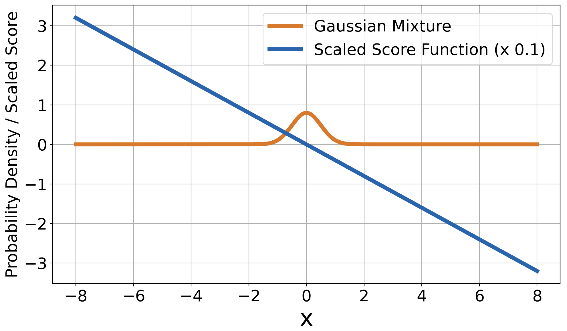
Refer to caption
Refer to caption
Figure 6: Probability densities and score functions for Gaussian distribution and Gaussian mixture distribution with two components. Here we scale the score function with 0.10.10.1 for better visibility.

A.3.3 ReLU activation with skip connection

Theorem A.5.

When σ𝜎\sigma is ReLU and V0𝑉0V\neq 0 , denote the optimal score matching objective value (2) with sθsubscript𝑠𝜃s_{\theta} specified in (3) as p,superscript𝑝p^{\star}, when mm𝑚superscript𝑚m\geq m^{*} and β1,𝛽1\beta\geq 1,

p=superscript𝑝absent\displaystyle p^{*}= miny12Ay22+bTy+c+2βy1,subscript𝑦12superscriptsubscriptnorm𝐴𝑦22superscript𝑏𝑇𝑦𝑐2𝛽subscriptnorm𝑦1\displaystyle\min_{y}\quad\frac{1}{2}\|Ay\|_{2}^{2}+b^{T}y+c+2\beta\|y\|_{1}\,, (18)

where m=y0superscript𝑚subscriptnormsuperscript𝑦0m^{*}=\|y^{*}\|_{0}, and ysuperscript𝑦y^{*} is any optimal solution to (18). A,b,c𝐴𝑏𝑐A,b,c and reconstruction rule for θ𝜃\theta is specficied in the proof below.

Proof.

Here we reduce score matching objective including ReLU activation to score matching objective including absolute value activation and exploits results in Theorem A.6. Let {wr,br,αr,vr}superscript𝑤𝑟superscript𝑏𝑟superscript𝛼𝑟superscript𝑣𝑟\{w^{r},b^{r},\alpha^{r},v^{r}\} denotes parameter set corresponding to ReLU activation, consider another parameter set {wa,ba,αa,va}superscript𝑤𝑎superscript𝑏𝑎superscript𝛼𝑎superscript𝑣𝑎\{w^{a},b^{a},\alpha^{a},v^{a}\} satisfying

{αr=2αa,wr=wa,br=ba,b0r=b0a12j=1mbjrαjr,vr=va12j=1mwjrαjr.casessuperscript𝛼𝑟2superscript𝛼𝑎otherwisesuperscript𝑤𝑟superscript𝑤𝑎otherwisesuperscript𝑏𝑟superscript𝑏𝑎otherwisesuperscriptsubscript𝑏0𝑟superscriptsubscript𝑏0𝑎12superscriptsubscript𝑗1𝑚superscriptsubscript𝑏𝑗𝑟superscriptsubscript𝛼𝑗𝑟otherwisesuperscript𝑣𝑟superscript𝑣𝑎12superscriptsubscript𝑗1𝑚superscriptsubscript𝑤𝑗𝑟superscriptsubscript𝛼𝑗𝑟otherwise\begin{cases}\alpha^{r}=2\alpha^{a},\\ w^{r}=w^{a},\\ b^{r}=b^{a},\\ b_{0}^{r}=b_{0}^{a}-\frac{1}{2}\sum_{j=1}^{m}b_{j}^{r}\alpha_{j}^{r},\\ v^{r}=v^{a}-\frac{1}{2}\sum_{j=1}^{m}w_{j}^{r}\alpha_{j}^{r}.\end{cases}

Then the score matching objective

minwr,αr,br,vr12j=1m(xwjr+1bjr)+αjr+xvr+1b0r22+1T(j=1mwjrαjr𝟙{xwjr+1bjr0})+nvr+β2j=1m(wjr2+αjr2)subscriptsuperscript𝑤𝑟superscript𝛼𝑟superscript𝑏𝑟superscript𝑣𝑟12superscriptsubscriptnormsuperscriptsubscript𝑗1𝑚subscript𝑥subscriptsuperscript𝑤𝑟𝑗1subscriptsuperscript𝑏𝑟𝑗subscriptsuperscript𝛼𝑟𝑗𝑥superscript𝑣𝑟1superscriptsubscript𝑏0𝑟22superscript1𝑇superscriptsubscript𝑗1𝑚subscriptsuperscript𝑤𝑟𝑗subscriptsuperscript𝛼𝑟𝑗1𝑥subscriptsuperscript𝑤𝑟𝑗1subscriptsuperscript𝑏𝑟𝑗0𝑛superscript𝑣𝑟𝛽2superscriptsubscript𝑗1𝑚superscriptsubscriptsuperscript𝑤𝑟𝑗2superscriptsubscriptsuperscript𝛼𝑟𝑗2\min_{w^{r},\alpha^{r},b^{r},v^{r}}\frac{1}{2}\left\|\sum_{j=1}^{m}(xw^{r}_{j}+1b^{r}_{j})_{+}\alpha^{r}_{j}+xv^{r}+1b_{0}^{r}\right\|_{2}^{2}+1^{T}\left(\sum_{j=1}^{m}w^{r}_{j}\alpha^{r}_{j}{\mathbbm{1}}\{xw^{r}_{j}+1b^{r}_{j}\geq 0\}\right)+nv^{r}+\frac{\beta}{2}\sum_{j=1}^{m}({w^{r}_{j}}^{2}+{\alpha^{r}_{j}}^{2})

is equivalent to

minwa,αa,ba,va12j=1m|xwja+1bja|αja+xva+1b0a22+1T(j=1mwjaαjasign(xwja+1bja))+nva+β2j=1m(wja2+4αja2).subscriptsuperscript𝑤𝑎superscript𝛼𝑎superscript𝑏𝑎superscript𝑣𝑎12delimited-‖|superscriptsubscript𝑗1𝑚𝑥subscriptsuperscript𝑤𝑎𝑗1subscriptsuperscript𝑏𝑎𝑗superscriptsubscriptdelimited-|‖subscriptsuperscript𝛼𝑎𝑗𝑥superscript𝑣𝑎1superscriptsubscript𝑏0𝑎22superscript1𝑇superscriptsubscript𝑗1𝑚subscriptsuperscript𝑤𝑎𝑗subscriptsuperscript𝛼𝑎𝑗sign𝑥subscriptsuperscript𝑤𝑎𝑗1subscriptsuperscript𝑏𝑎𝑗𝑛superscript𝑣𝑎𝛽2superscriptsubscript𝑗1𝑚superscriptsubscriptsuperscript𝑤𝑎𝑗24superscriptsubscriptsuperscript𝛼𝑎𝑗2\min_{w^{a},\alpha^{a},b^{a},v^{a}}\frac{1}{2}\left\|\sum_{j=1}^{m}|xw^{a}_{j}+1b^{a}_{j}|\alpha^{a}_{j}+xv^{a}+1b_{0}^{a}\right\|_{2}^{2}+1^{T}\left(\sum_{j=1}^{m}w^{a}_{j}\alpha^{a}_{j}{\mathrm{sign}}(xw^{a}_{j}+1b^{a}_{j})\right)+nv^{a}+\frac{\beta}{2}\sum_{j=1}^{m}\left({w^{a}_{j}}^{2}+4{\alpha^{a}_{j}}^{2}\right).

According to Lemma 2 in (Pilanci & Ergen, 2020), after rescaling, the above problem is equivalent to

minwa,αa,ba,va|wja|=112j=1m|xwja+1bja|αja+xva+1b0a22+1T(j=1mwjaαjasign(xwja+1bja))+nva+2βj=1m|αja|.subscriptsuperscript𝑤𝑎superscript𝛼𝑎superscript𝑏𝑎superscript𝑣𝑎subscriptsuperscript𝑤𝑎𝑗112delimited-‖|superscriptsubscript𝑗1𝑚𝑥subscriptsuperscript𝑤𝑎𝑗1subscriptsuperscript𝑏𝑎𝑗superscriptsubscriptdelimited-|‖subscriptsuperscript𝛼𝑎𝑗𝑥superscript𝑣𝑎1superscriptsubscript𝑏0𝑎22superscript1𝑇superscriptsubscript𝑗1𝑚subscriptsuperscript𝑤𝑎𝑗subscriptsuperscript𝛼𝑎𝑗sign𝑥subscriptsuperscript𝑤𝑎𝑗1subscriptsuperscript𝑏𝑎𝑗𝑛superscript𝑣𝑎2𝛽superscriptsubscript𝑗1𝑚subscriptsuperscript𝛼𝑎𝑗\min_{\begin{subarray}{c}w^{a},\alpha^{a},b^{a},v^{a}\\ |w^{a}_{j}|=1\end{subarray}}\frac{1}{2}\left\|\sum_{j=1}^{m}|xw^{a}_{j}+1b^{a}_{j}|\alpha^{a}_{j}+xv^{a}+1b_{0}^{a}\right\|_{2}^{2}+1^{T}\left(\sum_{j=1}^{m}w^{a}_{j}\alpha^{a}_{j}{\mathrm{sign}}(xw^{a}_{j}+1b^{a}_{j})\right)+nv^{a}+2\beta\sum_{j=1}^{m}|\alpha^{a}_{j}|. (19)

Following similar analysis as in Appendix A.3.4 with a different rescaling factor we can derive the convex program (18) with A=B12A1,b=A1T(nx¯/x¯22)+b1,c=n2/(2x¯22)formulae-sequence𝐴superscript𝐵12subscript𝐴1formulae-sequence𝑏superscriptsubscript𝐴1𝑇𝑛¯𝑥superscriptsubscriptnorm¯𝑥22subscript𝑏1𝑐superscript𝑛22superscriptsubscriptnorm¯𝑥22A=B^{\frac{1}{2}}A_{1},b=A_{1}^{T}(-n\bar{x}/\|\bar{x}\|_{2}^{2})+b_{1},c=-n^{2}/(2\|\bar{x}\|_{2}^{2}) where B=IPx¯𝐵𝐼subscript𝑃¯𝑥B=I-P_{\bar{x}} with Px¯=x¯x¯T/x¯22subscript𝑃¯𝑥¯𝑥superscript¯𝑥𝑇superscriptsubscriptnorm¯𝑥22P_{\bar{x}}=\bar{x}\bar{x}^{T}/\|\bar{x}\|_{2}^{2}, and A1,b1subscript𝐴1subscript𝑏1A_{1},b_{1} are identical to A,b𝐴𝑏A,b defined in Section A.3.1 respectively. Here, x¯j:=xjixi/nassignsubscript¯𝑥𝑗subscript𝑥𝑗subscript𝑖subscript𝑥𝑖𝑛\bar{x}_{j}:=x_{j}-\sum_{i}x_{i}/n denotes mean-subtracted data vector. The optimal solution set to (19) is given by

{wja=2|yj|,αja=|yj|/2,bja=2|yj|xj for j=1,,n,Wja=2|yj|,αja=|yj|/2,bja=2|yj|xjn for j=n+1,,2n,va=(x¯TA1y+n)/x¯22,b0a=1n1T([A1,A1]y+xva),casesformulae-sequenceformulae-sequencesuperscriptsubscriptsuperscript𝑤𝑎𝑗2subscriptsuperscript𝑦𝑗formulae-sequencesuperscriptsubscriptsuperscript𝛼𝑎𝑗subscriptsuperscript𝑦𝑗2superscriptsubscriptsuperscript𝑏𝑎𝑗2subscriptsuperscript𝑦𝑗subscript𝑥𝑗 for 𝑗1𝑛otherwiseformulae-sequenceformulae-sequencesuperscriptsubscriptsuperscript𝑊𝑎𝑗2subscriptsuperscript𝑦𝑗formulae-sequencesuperscriptsubscriptsuperscript𝛼𝑎𝑗subscriptsuperscript𝑦𝑗2superscriptsubscriptsuperscript𝑏𝑎𝑗2subscriptsuperscript𝑦𝑗subscript𝑥𝑗𝑛 for 𝑗𝑛12𝑛otherwisesuperscriptsuperscript𝑣𝑎superscript¯𝑥𝑇subscript𝐴1superscript𝑦𝑛superscriptsubscriptnorm¯𝑥22otherwisesuperscriptsuperscriptsubscript𝑏0𝑎1𝑛superscript1𝑇superscriptsubscript𝐴1superscriptsubscript𝐴1superscript𝑦𝑥superscriptsuperscript𝑣𝑎otherwise\begin{cases}{w^{a}_{j}}^{\star}=\sqrt{2|y^{\star}_{j}|},{\alpha^{a}_{j}}^{\star}=\sqrt{|y^{\star}_{j}|/2},{b^{a}_{j}}^{\star}=-\sqrt{2|y^{\star}_{j}|}x_{j}\text{ for }j=1,\ldots,n,\\ {W^{a}_{j}}^{\star}=-\sqrt{2|y^{\star}_{j}|},{\alpha^{a}_{j}}^{\star}=\sqrt{|y^{\star}_{j}|/2},{b^{a}_{j}}^{\star}=\sqrt{2|y^{\star}_{j}|}x_{j-n}\text{ for }j=n+1,\ldots,2n,\\ {v^{a}}^{\star}=-(\bar{x}^{T}A_{1}y^{\star}+n)/\|\bar{x}\|_{2}^{2},\\ {b_{0}^{a}}^{\star}=-\frac{1}{n}1^{T}([A_{1}^{\prime},A_{1}^{\prime}]y^{\star}+x{v^{a}}^{\star}),\end{cases}

where A1superscriptsubscript𝐴1A_{1}^{\prime} is A1subscript𝐴1A_{1} defined in Appendix A.3.1 and ysuperscript𝑦y^{\star} is optimal solution to convex program (18). Then the optimal parameter set {wr,br,αr,zr}superscript𝑤𝑟superscript𝑏𝑟superscript𝛼𝑟superscript𝑧𝑟\{w^{r},b^{r},\alpha^{r},z^{r}\} is given by

{wjr=2|yj|,αjr=2|yj|,bjr=2|yj|xj for j=1,,n,wjr=2|yj|,αjr=2|yj|,bjr=2|yj|xjn for j=n+1,,2n,vr=(x¯TA1y+n)/x¯22j=1mwjrαjr/2,b0r=1n1T([A1,A1]y+x((x¯TA1y+n)/x¯22))j=1mbjrαjr/2.casesformulae-sequenceformulae-sequencesuperscriptsubscriptsuperscript𝑤𝑟𝑗2subscriptsuperscript𝑦𝑗formulae-sequencesuperscriptsubscriptsuperscript𝛼𝑟𝑗2subscriptsuperscript𝑦𝑗superscriptsubscriptsuperscript𝑏𝑟𝑗2subscriptsuperscript𝑦𝑗subscript𝑥𝑗 for 𝑗1𝑛otherwiseformulae-sequenceformulae-sequencesuperscriptsubscriptsuperscript𝑤𝑟𝑗2subscriptsuperscript𝑦𝑗formulae-sequencesuperscriptsubscriptsuperscript𝛼𝑟𝑗2subscriptsuperscript𝑦𝑗superscriptsubscriptsuperscript𝑏𝑟𝑗2subscriptsuperscript𝑦𝑗subscript𝑥𝑗𝑛 for 𝑗𝑛12𝑛otherwisesuperscriptsuperscript𝑣𝑟superscript¯𝑥𝑇subscript𝐴1superscript𝑦𝑛superscriptsubscriptnorm¯𝑥22superscriptsubscript𝑗1𝑚superscriptsubscriptsuperscript𝑤𝑟𝑗superscriptsubscriptsuperscript𝛼𝑟𝑗2otherwisesuperscriptsuperscriptsubscript𝑏0𝑟1𝑛superscript1𝑇superscriptsubscript𝐴1superscriptsubscript𝐴1superscript𝑦𝑥superscript¯𝑥𝑇subscript𝐴1superscript𝑦𝑛superscriptsubscriptnorm¯𝑥22superscriptsubscript𝑗1𝑚superscriptsubscriptsuperscript𝑏𝑟𝑗superscriptsubscriptsuperscript𝛼𝑟𝑗2otherwise\begin{cases}{w^{r}_{j}}^{\star}=\sqrt{2|y^{\star}_{j}|},{\alpha^{r}_{j}}^{\star}=\sqrt{2|y^{\star}_{j}|},{b^{r}_{j}}^{\star}=-\sqrt{2|y^{\star}_{j}|}x_{j}\text{ for }j=1,\ldots,n,\\ {w^{r}_{j}}^{\star}=-\sqrt{2|y^{\star}_{j}|},{\alpha^{r}_{j}}^{\star}=\sqrt{2|y^{\star}_{j}|},{b^{r}_{j}}^{\star}=\sqrt{2|y^{\star}_{j}|}x_{j-n}\text{ for }j=n+1,\ldots,2n,\\ {v^{r}}^{\star}=-(\bar{x}^{T}A_{1}y^{\star}+n)/\|\bar{x}\|_{2}^{2}-\sum_{j=1}^{m}{w^{r}_{j}}^{\star}{\alpha^{r}_{j}}^{\star}/2,\\ {b_{0}^{r}}^{\star}=-\frac{1}{n}1^{T}([A_{1}^{\prime},A_{1}^{\prime}]y^{\star}+x(-(\bar{x}^{T}A_{1}y^{\star}+n)/\|\bar{x}\|_{2}^{2}))-\sum_{j=1}^{m}{b^{r}_{j}}^{\star}{\alpha^{r}_{j}}^{\star}/2.\end{cases}

A.3.4 Absolute value activation with skip connection

Theorem A.6.

When σ𝜎\sigma is absolute value activation and V0𝑉0V\neq 0 , denote the optimal score matching objective value (2) with sθsubscript𝑠𝜃s_{\theta} specified in (3) as p,superscript𝑝p^{\star}, when mm𝑚superscript𝑚m\geq m^{*} and β2,𝛽2\beta\geq 2,

p=superscript𝑝absent\displaystyle p^{*}= miny12Ay22+bTy+βy1,subscript𝑦12superscriptsubscriptnorm𝐴𝑦22superscript𝑏𝑇𝑦𝛽subscriptnorm𝑦1\displaystyle\min_{y}\quad\frac{1}{2}\|Ay\|_{2}^{2}+b^{T}y+\beta\|y\|_{1}\,, (20)

where m=y0superscript𝑚subscriptnormsuperscript𝑦0m^{*}=\|y^{*}\|_{0}, and ysuperscript𝑦y^{*} is any optimal solution to (20). A,b𝐴𝑏A,b and reconstruction rule for θ𝜃\theta is specficied in the proof below.

Proof.

Consider data matrix xn𝑥superscript𝑛x\in\mathbb{R}^{n}, then the score matching objective is reduced to

p=minw,α,b,v12j=1m|xwj+1bj|αj+xv+1b022+1T(j=1mwjαjsign(xwj+1bj))+nv+12βj=1m(wj2+αj2).superscript𝑝subscript𝑤𝛼𝑏𝑣12delimited-‖|superscriptsubscript𝑗1𝑚𝑥subscript𝑤𝑗1subscript𝑏𝑗superscriptsubscriptdelimited-|‖subscript𝛼𝑗𝑥𝑣1subscript𝑏022superscript1𝑇superscriptsubscript𝑗1𝑚subscript𝑤𝑗subscript𝛼𝑗sign𝑥subscript𝑤𝑗1subscript𝑏𝑗𝑛𝑣12𝛽superscriptsubscript𝑗1𝑚superscriptsubscript𝑤𝑗2superscriptsubscript𝛼𝑗2p^{\star}=\min_{w,\alpha,b,v}\frac{1}{2}\left\|\sum_{j=1}^{m}|xw_{j}+1b_{j}|\alpha_{j}+xv+1b_{0}\right\|_{2}^{2}+1^{T}\left(\sum_{j=1}^{m}w_{j}\alpha_{j}{\mathrm{sign}}(xw_{j}+1b_{j})\right)+nv+\frac{1}{2}\beta\sum_{j=1}^{m}(w_{j}^{2}+\alpha_{j}^{2}).

Following similar analysis as in Appendix A.3.1, we can derive the dual problem as

d=maxz1,z2minw,α,b,v,r1,r2|wj|=112r122+1Tr2+nv+βj=1m|αj|+z1T(r1j=1m|xwj+1bj|αjxv1b0)superscript𝑑subscriptsubscript𝑧1subscript𝑧2subscript𝑤𝛼𝑏𝑣subscript𝑟1subscript𝑟2subscript𝑤𝑗112superscriptsubscriptnormsubscript𝑟122superscript1𝑇subscript𝑟2𝑛𝑣𝛽superscriptsubscript𝑗1𝑚subscript𝛼𝑗superscriptsubscript𝑧1𝑇subscript𝑟1superscriptsubscript𝑗1𝑚𝑥subscript𝑤𝑗1subscript𝑏𝑗subscript𝛼𝑗𝑥𝑣1subscript𝑏0\displaystyle d^{\star}=\max_{z_{1},z_{2}}\min_{\begin{subarray}{c}w,\alpha,b,v,r_{1},r_{2}\\ |w_{j}|=1\end{subarray}}\frac{1}{2}\|r_{1}\|_{2}^{2}+1^{T}r_{2}+nv+\beta\sum_{j=1}^{m}|\alpha_{j}|+z_{1}^{T}\left(r_{1}-\sum_{j=1}^{m}|xw_{j}+1b_{j}|\alpha_{j}-xv-1b_{0}\right)
+z2T(r2j=1mwjαjsign(xwj+1bj)).superscriptsubscript𝑧2𝑇subscript𝑟2superscriptsubscript𝑗1𝑚subscript𝑤𝑗subscript𝛼𝑗sign𝑥subscript𝑤𝑗1subscript𝑏𝑗\displaystyle\qquad\qquad\qquad\qquad\qquad\qquad\qquad\qquad\qquad\qquad\qquad\qquad+z_{2}^{T}\left(r_{2}-\sum_{j=1}^{m}w_{j}\alpha_{j}{\mathrm{sign}}(xw_{j}+1b_{j})\right).

which gives a lower bound of psuperscript𝑝p^{\star}. Minimizing over r1subscript𝑟1r_{1} and r2subscript𝑟2r_{2} gives

maxz1minw,α,b,v|wj|=112z122+nv+βj=1m|αj|z1T(j=1m|xwj+1bj|αj+xv+1b0)+1Tj=1mwjαjsign(xwj+1bj).subscriptsubscript𝑧1subscript𝑤𝛼𝑏𝑣subscript𝑤𝑗112superscriptsubscriptnormsubscript𝑧122𝑛𝑣𝛽superscriptsubscript𝑗1𝑚subscript𝛼𝑗superscriptsubscript𝑧1𝑇superscriptsubscript𝑗1𝑚𝑥subscript𝑤𝑗1subscript𝑏𝑗subscript𝛼𝑗𝑥𝑣1subscript𝑏0superscript1𝑇superscriptsubscript𝑗1𝑚subscript𝑤𝑗subscript𝛼𝑗sign𝑥subscript𝑤𝑗1subscript𝑏𝑗\max_{z_{1}}\min_{\begin{subarray}{c}w,\alpha,b,v\\ |w_{j}|=1\end{subarray}}-\frac{1}{2}\|z_{1}\|_{2}^{2}+nv+\beta\sum_{j=1}^{m}|\alpha_{j}|-z_{1}^{T}\left(\sum_{j=1}^{m}|xw_{j}+1b_{j}|\alpha_{j}+xv+1b_{0}\right)+1^{T}\sum_{j=1}^{m}w_{j}\alpha_{j}{\mathrm{sign}}(xw_{j}+1b_{j}).

Minimizing over v𝑣v gives

maxz1z1Tx=nminw,α,b|wj|=112z122+βj=1m|αj|z1T(j=1m|xwj+1bj|αj+1b0)+1Tj=1mwjαjsign(xwj+1bj).subscriptsubscript𝑧1superscriptsubscript𝑧1𝑇𝑥𝑛subscript𝑤𝛼𝑏subscript𝑤𝑗112superscriptsubscriptnormsubscript𝑧122𝛽superscriptsubscript𝑗1𝑚subscript𝛼𝑗superscriptsubscript𝑧1𝑇superscriptsubscript𝑗1𝑚𝑥subscript𝑤𝑗1subscript𝑏𝑗subscript𝛼𝑗1subscript𝑏0superscript1𝑇superscriptsubscript𝑗1𝑚subscript𝑤𝑗subscript𝛼𝑗sign𝑥subscript𝑤𝑗1subscript𝑏𝑗\max_{\begin{subarray}{c}z_{1}\\ z_{1}^{T}x=n\end{subarray}}\min_{\begin{subarray}{c}w,\alpha,b\\ |w_{j}|=1\end{subarray}}-\frac{1}{2}\|z_{1}\|_{2}^{2}+\beta\sum_{j=1}^{m}|\alpha_{j}|-z_{1}^{T}\left(\sum_{j=1}^{m}|xw_{j}+1b_{j}|\alpha_{j}+1b_{0}\right)+1^{T}\sum_{j=1}^{m}w_{j}\alpha_{j}{\mathrm{sign}}(xw_{j}+1b_{j}).

Minimizing over αjsubscript𝛼𝑗\alpha_{j} gives

maxzsubscript𝑧\displaystyle\max_{z} minb012z22b0zT1subscriptsubscript𝑏012superscriptsubscriptnorm𝑧22subscript𝑏0superscript𝑧𝑇1\displaystyle\min_{b_{0}}-\frac{1}{2}\|z\|_{2}^{2}-b_{0}z^{T}1
s.t. {zTx=n|zT|xwj+1bj|wj1Tsign(xwj+1bj)|β,|wj|=1,bj.s.t. casessuperscript𝑧𝑇𝑥𝑛otherwiseformulae-sequencesuperscript𝑧𝑇𝑥subscript𝑤𝑗1subscript𝑏𝑗subscript𝑤𝑗superscript1𝑇sign𝑥subscript𝑤𝑗1subscript𝑏𝑗𝛽for-allsubscript𝑤𝑗1for-allsubscript𝑏𝑗otherwise\displaystyle\mbox{s.t. }\begin{cases}z^{T}x=n\\ |z^{T}|xw_{j}+1b_{j}|-w_{j}1^{T}{\mathrm{sign}}(xw_{j}+1b_{j})|\leq\beta,\quad\forall|w_{j}|=1,\forall b_{j}.\end{cases}

Following same logic as in Appendix A.3.1, the above problem is equivalent to

maxz12z22subscript𝑧12superscriptsubscriptnorm𝑧22\displaystyle\max_{z}\quad-\frac{1}{2}\|z\|_{2}^{2} (21)
s.t.{|zT|x1xi|1Tsign(x1xi)|β|zT|x+1xi|+1Tsign(x+1xi)|βzT1=0zTx=ni=1,,n.s.t.casessuperscript𝑧𝑇𝑥1subscript𝑥𝑖superscript1𝑇sign𝑥1subscript𝑥𝑖𝛽otherwisesuperscript𝑧𝑇𝑥1subscript𝑥𝑖superscript1𝑇sign𝑥1subscript𝑥𝑖𝛽otherwisesuperscript𝑧𝑇10otherwisesuperscript𝑧𝑇𝑥𝑛otherwisefor-all𝑖1𝑛\displaystyle\mbox{s.t.}\begin{cases}|z^{T}|x-1x_{i}|-1^{T}{\mathrm{sign}}(x-1x_{i})|\leq\beta\quad\\ |z^{T}|-x+1x_{i}|+1^{T}{\mathrm{sign}}(-x+1x_{i})|\leq\beta\quad\\ z^{T}1=0\\ z^{T}x=n\end{cases}\forall i=1,\ldots,n.

According to Lemma A.3, when β2,𝛽2\beta\geq 2, the constraints in (21) are feasible for affine constraints, thus Slater’s condition holds and the dual problem writes

d=minz0,z1,z2,z3,z4,z5s.t.z0,z1,z2,z30maxz12z22+i=1nz0i(zT|x1xi|1Tsign(x1xi)+β)superscript𝑑subscriptsubscript𝑧0subscript𝑧1subscript𝑧2subscript𝑧3subscript𝑧4subscript𝑧5s.t.subscript𝑧0subscript𝑧1subscript𝑧2subscript𝑧30subscript𝑧12superscriptsubscriptnorm𝑧22superscriptsubscript𝑖1𝑛subscript𝑧0𝑖superscript𝑧𝑇𝑥1subscript𝑥𝑖superscript1𝑇sign𝑥1subscript𝑥𝑖𝛽\displaystyle d^{\star}=\min_{\begin{subarray}{c}z_{0},z_{1},z_{2},z_{3},z_{4},z_{5}\\ \mbox{s.t.}z_{0},z_{1},z_{2},z_{3}\geq 0\end{subarray}}\max_{z}-\frac{1}{2}\|z\|_{2}^{2}+\sum_{i=1}^{n}z_{0i}\left(z^{T}|x-1x_{i}|-1^{T}{\mathrm{sign}}(x-1x_{i})+\beta\right)
+i=1nz1i(zT|x1xi|+1Tsign(x1xi)+β)superscriptsubscript𝑖1𝑛subscript𝑧1𝑖superscript𝑧𝑇𝑥1subscript𝑥𝑖superscript1𝑇sign𝑥1subscript𝑥𝑖𝛽\displaystyle\qquad\qquad\qquad\qquad\qquad+\sum_{i=1}^{n}z_{1i}\left(-z^{T}|x-1x_{i}|+1^{T}{\mathrm{sign}}(x-1x_{i})+\beta\right)
+i=1nz2i(zT|x+1xi|+1Tsign(x+1xi)+β)superscriptsubscript𝑖1𝑛subscript𝑧2𝑖superscript𝑧𝑇𝑥1subscript𝑥𝑖superscript1𝑇sign𝑥1subscript𝑥𝑖𝛽\displaystyle\qquad\qquad\qquad\qquad\qquad+\sum_{i=1}^{n}z_{2i}\left(z^{T}|-x+1x_{i}|+1^{T}{\mathrm{sign}}(-x+1x_{i})+\beta\right)
+i=1nz3i(zT|x+1xi|1Tsign(x+1xi)+β)superscriptsubscript𝑖1𝑛subscript𝑧3𝑖superscript𝑧𝑇𝑥1subscript𝑥𝑖superscript1𝑇sign𝑥1subscript𝑥𝑖𝛽\displaystyle\qquad\qquad\qquad\qquad\qquad+\sum_{i=1}^{n}z_{3i}\left(-z^{T}|-x+1x_{i}|-1^{T}{\mathrm{sign}}(-x+1x_{i})+\beta\right)
+z4(zTxn)+z5zT1,subscript𝑧4superscript𝑧𝑇𝑥𝑛subscript𝑧5superscript𝑧𝑇1\displaystyle\qquad\qquad\qquad\qquad\qquad+z_{4}(z^{T}x-n)+z_{5}z^{T}1,

which is equivalent to

minz0,z1,z2,z3,z4,z5s.t.z0,z1,z2,z30maxz12z22+eTz+f,subscriptsubscript𝑧0subscript𝑧1subscript𝑧2subscript𝑧3subscript𝑧4subscript𝑧5s.t.subscript𝑧0subscript𝑧1subscript𝑧2subscript𝑧30subscript𝑧12superscriptsubscriptnorm𝑧22superscript𝑒𝑇𝑧𝑓\displaystyle\min_{\begin{subarray}{c}z_{0},z_{1},z_{2},z_{3},z_{4},z_{5}\\ \mbox{s.t.}z_{0},z_{1},z_{2},z_{3}\geq 0\end{subarray}}\max_{z}-\frac{1}{2}\|z\|_{2}^{2}+e^{T}z+f,

where

e=i=1nz0i|x1xi|i=1nz1i|x1xi|+i=1nz2i|x+1xi|i=1nz3i|x+1xi|+xz4+1z5,𝑒superscriptsubscript𝑖1𝑛subscript𝑧0𝑖𝑥1subscript𝑥𝑖superscriptsubscript𝑖1𝑛subscript𝑧1𝑖𝑥1subscript𝑥𝑖superscriptsubscript𝑖1𝑛subscript𝑧2𝑖𝑥1subscript𝑥𝑖superscriptsubscript𝑖1𝑛subscript𝑧3𝑖𝑥1subscript𝑥𝑖𝑥subscript𝑧41subscript𝑧5e=\sum_{i=1}^{n}z_{0i}|x-1x_{i}|-\sum_{i=1}^{n}z_{1i}|x-1x_{i}|+\sum_{i=1}^{n}z_{2i}|-x+1x_{i}|-\sum_{i=1}^{n}z_{3i}|-x+1x_{i}|+xz_{4}+1z_{5},

and

f=i=1nz0i1Tsign(x1xi)+i=1nz1i1Tsign(x1xi)+i=1nz2i1Tsign(x+1xi)𝑓superscriptsubscript𝑖1𝑛subscript𝑧0𝑖superscript1𝑇sign𝑥1subscript𝑥𝑖superscriptsubscript𝑖1𝑛subscript𝑧1𝑖superscript1𝑇sign𝑥1subscript𝑥𝑖superscriptsubscript𝑖1𝑛subscript𝑧2𝑖superscript1𝑇sign𝑥1subscript𝑥𝑖\displaystyle f=-\sum_{i=1}^{n}z_{0i}1^{T}{\mathrm{sign}}(x-1x_{i})+\sum_{i=1}^{n}z_{1i}1^{T}{\mathrm{sign}}(x-1x_{i})+\sum_{i=1}^{n}z_{2i}1^{T}{\mathrm{sign}}(-x+1x_{i})
i=1nz3i1Tsign(x+1xi)z4n+β(z01+z11+z21+z31).superscriptsubscript𝑖1𝑛subscript𝑧3𝑖superscript1𝑇sign𝑥1subscript𝑥𝑖subscript𝑧4𝑛𝛽subscriptnormsubscript𝑧01subscriptnormsubscript𝑧11subscriptnormsubscript𝑧21subscriptnormsubscript𝑧31\displaystyle-\sum_{i=1}^{n}z_{3i}1^{T}{\mathrm{sign}}(-x+1x_{i})-z_{4}n+\beta(\|z_{0}\|_{1}+\|z_{1}\|_{1}+\|z_{2}\|_{1}+\|z_{3}\|_{1}).

Maximizing over z𝑧z gives

minz0,z1,z2,z3,z4,z5s.t.z0,z1,z2,z3012e22+f.subscriptsubscript𝑧0subscript𝑧1subscript𝑧2subscript𝑧3subscript𝑧4subscript𝑧5s.t.subscript𝑧0subscript𝑧1subscript𝑧2subscript𝑧3012superscriptsubscriptnorm𝑒22𝑓\displaystyle\min_{\begin{subarray}{c}z_{0},z_{1},z_{2},z_{3},z_{4},z_{5}\\ \mbox{s.t.}z_{0},z_{1},z_{2},z_{3}\geq 0\end{subarray}}\frac{1}{2}\|e\|_{2}^{2}+f.

Simplifying to get

miny0,y1,y2,y312A1(y0+y1)+xy2+1y322+1TC1y01TC2y1+ny2+β(y11+y21),subscriptsubscript𝑦0subscript𝑦1subscript𝑦2subscript𝑦312superscriptsubscriptnormsuperscriptsubscript𝐴1subscript𝑦0subscript𝑦1𝑥subscript𝑦21subscript𝑦322superscript1𝑇subscript𝐶1subscript𝑦0superscript1𝑇subscript𝐶2subscript𝑦1𝑛subscript𝑦2𝛽subscriptnormsubscript𝑦11subscriptnormsubscript𝑦21\displaystyle\min_{y_{0},y_{1},y_{2},y_{3}}\frac{1}{2}\left\|A_{1}^{\prime}(y_{0}+y_{1})+xy_{2}+1y_{3}\right\|_{2}^{2}+1^{T}C_{1}y_{0}-1^{T}C_{2}y_{1}+ny_{2}+\beta(\|y_{1}\|_{1}+\|y_{2}\|_{1}), (22)

where A1,C1,C2superscriptsubscript𝐴1subscript𝐶1subscript𝐶2A_{1}^{\prime},C_{1},C_{2} are as A1,C1,C2subscript𝐴1subscript𝐶1subscript𝐶2A_{1},C_{1},C_{2} defined in Appendix A.3.1. Minimizing over y3subscript𝑦3y_{3} gives y3=1T(A1(y0+y1)+xy2)/nsubscript𝑦3superscript1𝑇superscriptsubscript𝐴1subscript𝑦0subscript𝑦1𝑥subscript𝑦2𝑛y_{3}=-1^{T}(A_{1}^{\prime}(y_{0}+y_{1})+xy_{2})/n and (22) is reduced to

miny0,y1,y212A¯1(y0+y1)+x¯y222+1TC1y01TC2y1+ny2+β(y11+y21),subscriptsubscript𝑦0subscript𝑦1subscript𝑦212superscriptsubscriptnormsuperscriptsubscript¯𝐴1subscript𝑦0subscript𝑦1¯𝑥subscript𝑦222superscript1𝑇subscript𝐶1subscript𝑦0superscript1𝑇subscript𝐶2subscript𝑦1𝑛subscript𝑦2𝛽subscriptnormsubscript𝑦11subscriptnormsubscript𝑦21\min_{y_{0},y_{1},y_{2}}\frac{1}{2}\left\|\bar{A}_{1}^{\prime}(y_{0}+y_{1})+\bar{x}y_{2}\right\|_{2}^{2}+1^{T}C_{1}y_{0}-1^{T}C_{2}y_{1}+ny_{2}+\beta(\|y_{1}\|_{1}+\|y_{2}\|_{1}),

where A¯1superscriptsubscript¯𝐴1\bar{A}_{1}^{\prime} is as A¯1subscript¯𝐴1\bar{A}_{1} defined in Appendix A.3.1. Minimizing over y2subscript𝑦2y_{2} gives y2=(x¯TA¯1(y0+y1)+n)/x¯22subscript𝑦2superscript¯𝑥𝑇superscriptsubscript¯𝐴1subscript𝑦0subscript𝑦1𝑛superscriptsubscriptnorm¯𝑥22y_{2}=-\left(\bar{x}^{T}\bar{A}_{1}^{\prime}(y_{0}+y_{1})+n\right)/\|\bar{x}\|_{2}^{2} and the above problem is equivalent to the convex program (20) in Theorem A.6 with A=B12A1,b=A1T(nx¯/x¯22)+b1,c=n2/(2x¯22)formulae-sequence𝐴superscript𝐵12subscript𝐴1formulae-sequence𝑏superscriptsubscript𝐴1𝑇𝑛¯𝑥superscriptsubscriptnorm¯𝑥22subscript𝑏1𝑐superscript𝑛22superscriptsubscriptnorm¯𝑥22A=B^{\frac{1}{2}}A_{1},b=A_{1}^{T}(-n\bar{x}/\|\bar{x}\|_{2}^{2})+b_{1},c=-n^{2}/(2\|\bar{x}\|_{2}^{2}) where B=IPx¯𝐵𝐼subscript𝑃¯𝑥B=I-P_{\bar{x}} with Px¯=x¯x¯T/x¯22subscript𝑃¯𝑥¯𝑥superscript¯𝑥𝑇superscriptsubscriptnorm¯𝑥22P_{\bar{x}}=\bar{x}\bar{x}^{T}/\|\bar{x}\|_{2}^{2}, and A1,b1subscript𝐴1subscript𝑏1A_{1},b_{1} are identical to A,b𝐴𝑏A,b defined in Section A.3.1 respectively. Once we obtain optimal solution ysuperscript𝑦y^{\star} to problem (20), we can take

{wj=|yj|,αj=|yj|,bj=|yj|xj for j=1,,n,wj=|yj|,αj=|yj|,bj=|yj|xjn for j=n+1,,2n,v=(x¯TA1y+n)/x¯22,b0=1n1T([A1,A1]y+xv),casesformulae-sequenceformulae-sequencesuperscriptsubscript𝑤𝑗subscriptsuperscript𝑦𝑗formulae-sequencesuperscriptsubscript𝛼𝑗subscriptsuperscript𝑦𝑗subscriptsuperscript𝑏𝑗subscriptsuperscript𝑦𝑗subscript𝑥𝑗 for 𝑗1𝑛otherwiseformulae-sequenceformulae-sequencesuperscriptsubscript𝑤𝑗subscriptsuperscript𝑦𝑗formulae-sequencesuperscriptsubscript𝛼𝑗subscriptsuperscript𝑦𝑗subscriptsuperscript𝑏𝑗subscriptsuperscript𝑦𝑗subscript𝑥𝑗𝑛 for 𝑗𝑛12𝑛otherwisesuperscript𝑣superscript¯𝑥𝑇subscript𝐴1superscript𝑦𝑛superscriptsubscriptnorm¯𝑥22otherwisesuperscriptsubscript𝑏01𝑛superscript1𝑇superscriptsubscript𝐴1superscriptsubscript𝐴1superscript𝑦𝑥superscript𝑣otherwise\begin{cases}w_{j}^{\star}=\sqrt{|y^{\star}_{j}|},\alpha_{j}^{\star}=\sqrt{|y^{\star}_{j}|},b^{\star}_{j}=-\sqrt{|y^{\star}_{j}|}x_{j}\text{ for }j=1,\ldots,n,\\ w_{j}^{\star}=-\sqrt{|y^{\star}_{j}|},\alpha_{j}^{\star}=\sqrt{|y^{\star}_{j}|},b^{\star}_{j}=\sqrt{|y^{\star}_{j}|}x_{j-n}\text{ for }j=n+1,\ldots,2n,\\ v^{\star}=-(\bar{x}^{T}A_{1}y^{\star}+n)/\|\bar{x}\|_{2}^{2},\\ b_{0}^{\star}=-\frac{1}{n}1^{T}([A_{1}^{\prime},A_{1}^{\prime}]y^{\star}+xv^{\star}),\end{cases}

then score matching objective has the same value as optimal value of convex program (20), which indicates p=dsuperscript𝑝superscript𝑑p^{\star}=d^{\star} and the above parameter set is optimal.

A.4 Explanation for Unbounded Objective Value

Here we illustrate via a simple example that weight decay is necessary for the optimal objective value to stay finite. Follow notation in Appendix A.2, consider for example only one data point and one hidden neuron, then objective function for the neural network with ReLU activation and no skip connection would be

12((xw+b)+α+b0)2+wα𝟙(xw+b0)+β2(w2+α2).12superscriptsubscript𝑥𝑤𝑏𝛼subscript𝑏02𝑤𝛼1𝑥𝑤𝑏0𝛽2superscript𝑤2superscript𝛼2\frac{1}{2}((xw+b)_{+}\alpha+b_{0})^{2}+w\alpha{\mathbbm{1}}(xw+b\geq 0)+\frac{\beta}{2}(w^{2}+\alpha^{2}).

WLOG consider x=1,𝑥1x=1, then when weight decay parameter 0β<1,0𝛽10\leq\beta<1, set b=w+1β𝑏𝑤1𝛽b=-w+\sqrt{1-\beta} and b0=0subscript𝑏00b_{0}=0 above, we get

1β2α2+wα+β2(w2+α2).1𝛽2superscript𝛼2𝑤𝛼𝛽2superscript𝑤2superscript𝛼2\frac{1-\beta}{2}\alpha^{2}+w\alpha+\frac{\beta}{2}(w^{2}+\alpha^{2}).

Then we can set α=w𝛼𝑤\alpha=-w and the above expression becomes (β1)w2/2𝛽1superscript𝑤22(\beta-1)w^{2}/2. Thus the objective goes to minus infinity when w𝑤w goes to infinity.

A.5 Proof in Section 3.3

Proof.

The optimality condition for convex program (4) is

0ATAy+b+βθ1,0superscript𝐴𝑇𝐴𝑦𝑏𝛽subscript𝜃10\in A^{T}Ay+b+\beta\theta_{1}, (23)

where θ1y1subscript𝜃1subscriptnorm𝑦1\theta_{1}\in\partial\|y\|_{1}. To show ysuperscript𝑦y^{\star} satisfies optimality condition (23), let aisubscript𝑎𝑖a_{i} denote the i𝑖ith column of A𝐴A. Check the first entry,

a1TAy+b1+β(1)=nvy1nvy3n+nβ=0.superscriptsubscript𝑎1𝑇𝐴𝑦subscript𝑏1𝛽1𝑛𝑣subscriptsuperscript𝑦1𝑛𝑣subscriptsuperscript𝑦3𝑛𝑛𝛽0\displaystyle\quad a_{1}^{T}Ay+b_{1}+\beta(-1)=nvy^{\star}_{1}-nvy^{\star}_{3n}+n-\beta=0.

Check the 3n3𝑛3nth entry,

a3nTAy+b3n+β=nvy1+nvy3nn+β=0.superscriptsubscript𝑎3𝑛𝑇𝐴𝑦subscript𝑏3𝑛𝛽𝑛𝑣subscriptsuperscript𝑦1𝑛𝑣subscriptsuperscript𝑦3𝑛𝑛𝛽0\displaystyle\quad a_{3n}^{T}Ay+b_{3n}+\beta=-nvy^{\star}_{1}+nvy^{\star}_{3n}-n+\beta=0.

For j𝑗jth entry with j{1,3n}𝑗13𝑛j\not\in\{1,3n\}, note

|ajTAy+bj|superscriptsubscript𝑎𝑗𝑇𝐴𝑦subscript𝑏𝑗\displaystyle\quad|a_{j}^{T}Ay+b_{j}|
=|ajT(a1y1+a3ny3n)+bj|absentsuperscriptsubscript𝑎𝑗𝑇subscript𝑎1subscriptsuperscript𝑦1subscript𝑎3𝑛subscriptsuperscript𝑦3𝑛subscript𝑏𝑗\displaystyle=|a_{j}^{T}(a_{1}y^{\star}_{1}+a_{3n}y^{\star}_{3n})+b_{j}|
=|ajT(a1y1a1y3n)+bj|absentsuperscriptsubscript𝑎𝑗𝑇subscript𝑎1subscriptsuperscript𝑦1subscript𝑎1subscriptsuperscript𝑦3𝑛subscript𝑏𝑗\displaystyle=|a_{j}^{T}(a_{1}y^{\star}_{1}-a_{1}y^{\star}_{3n})+b_{j}|
=|βnnvajTa1+bj|.absent𝛽𝑛𝑛𝑣superscriptsubscript𝑎𝑗𝑇subscript𝑎1subscript𝑏𝑗\displaystyle=\left|\frac{\beta-n}{nv}a_{j}^{T}a_{1}+b_{j}\right|.

Since |bj|n1subscript𝑏𝑗𝑛1|b_{j}|\leq n-1, by continuity, |ajTAy+bj|βsuperscriptsubscript𝑎𝑗𝑇𝐴𝑦subscript𝑏𝑗𝛽|a_{j}^{T}Ay+b_{j}|\leq\beta should hold as we decrease β𝛽\beta a little further to threshold β1=maxj{1,3n}|ajTAy+bj|subscript𝛽1subscript𝑗13𝑛superscriptsubscript𝑎𝑗𝑇𝐴𝑦subscript𝑏𝑗\beta_{1}=\max_{j\not\in\{1,3n\}}|a_{j}^{T}Ay+b_{j}|. Therefore, ysuperscript𝑦y^{\star} is optimal.

A.6 Supplementary Case Studies

A.6.1 Absolute value activation without skip connection

In this section, we show that convex program (14) can be solved analytically for certain weight decay range and the predicted score function may not be compliant with log-concave sampling convergence theory. When β>b,𝛽subscriptnorm𝑏\beta>\|b\|_{\infty}, y=0𝑦0y=0 is optimal and the predicted score is always zero. When β𝛽\beta is decreased further to some threshold β2<nsubscript𝛽2𝑛\beta_{2}<n, i.e., when β2<βnsubscript𝛽2𝛽𝑛\beta_{2}<\beta\leq n, then

y𝑦\displaystyle y =[βn2nv+t,0,,0,nβ2nv+t]Tabsentsuperscriptmatrix𝛽𝑛2𝑛𝑣𝑡00𝑛𝛽2𝑛𝑣𝑡𝑇\displaystyle=\begin{bmatrix}\frac{\beta-n}{2nv}+t,&0,&\ldots,&0,&\frac{n-\beta}{2nv}+t\end{bmatrix}^{T}

is optimal with any t𝑡t\in\mathbb{R} such that |t|nβ2nv𝑡𝑛𝛽2𝑛𝑣|t|\leq\frac{n-\beta}{2nv} where μ𝜇\mu and v𝑣v denotes the sample mean and sample variance as described in Section 3.3 555See Appendix A.7.1 for proof and value of β2subscript𝛽2\beta_{2}.. For any test data x^^𝑥\hat{x}, the corresponding predicted score y^^𝑦\hat{y} is given by

{y^=βnnv(x^μ),x1x^xny^=2tx^+(βnnv+2t)x1+nβnvμ,x^<x1y^=2tx^(nβnv+2t)xn+nβnvμ.x^>xncases^𝑦𝛽𝑛𝑛𝑣^𝑥𝜇subscript𝑥1^𝑥subscript𝑥𝑛^𝑦2𝑡^𝑥𝛽𝑛𝑛𝑣2𝑡subscript𝑥1𝑛𝛽𝑛𝑣𝜇^𝑥subscript𝑥1^𝑦2𝑡^𝑥𝑛𝛽𝑛𝑣2𝑡subscript𝑥𝑛𝑛𝛽𝑛𝑣𝜇^𝑥subscript𝑥𝑛\begin{cases}\hat{y}=\frac{\beta-n}{nv}(\hat{x}-\mu),\quad&x_{1}\leq\hat{x}\leq x_{n}\\ \hat{y}=-2t\hat{x}+(\frac{\beta-n}{nv}+2t)x_{1}+\frac{n-\beta}{nv}\mu,\quad&\hat{x}<x_{1}\\ \hat{y}=2t\hat{x}-(\frac{n-\beta}{nv}+2t)x_{n}+\frac{n-\beta}{nv}\mu.\quad&\hat{x}>x_{n}\end{cases} (24)
Theorem A.7.

(Convergence Result) When sθsubscript𝑠𝜃s_{\theta} is of two-layer neural network with absolute value activation and β2<βn,subscript𝛽2𝛽𝑛\beta_{2}<\beta\leq n, let π1superscript𝜋1\pi^{1} denote the target distribution (defined below). For any ϵ[0,1]italic-ϵ01\epsilon\in[0,1], if we take step size ηϵ2nvnβ,asymptotically-equals𝜂superscriptitalic-ϵ2𝑛𝑣𝑛𝛽\eta\asymp\frac{\epsilon^{2}nv}{n-\beta}, then for the mixture distribution μ¯=T1t=1Txt¯𝜇superscript𝑇1superscriptsubscript𝑡1𝑇superscript𝑥𝑡\overline{\mu}=T^{-1}\sum_{t=1}^{T}x^{t}, it holds that KL(μ¯π1)ϵKLconditional¯𝜇superscript𝜋1italic-ϵ\sqrt{\text{KL}(\overline{\mu}\|\pi^{1})}\leq\epsilon after

O((nβ)W22(μ0,π1)nvϵ4)iterations,𝑂𝑛𝛽superscriptsubscript𝑊22subscript𝜇0superscript𝜋1𝑛𝑣superscriptitalic-ϵ4iterationsO\left(\frac{(n-\beta)W_{2}^{2}(\mu_{0},\pi^{1})}{nv\epsilon^{4}}\right)\quad\text{iterations},

where W2subscript𝑊2W_{2} denotes 2-Wasserstein distance and π1superscript𝜋1\pi^{1} satisfies

π1{exp(βnnv(x1μ)x+nβ2nvx12),x<x1,exp(βn2nvx2μ(βn)nvx),x1xxn,exp(βnnv(xnμ)x+nβ2nvxn2),xxn.proportional-tosuperscript𝜋1cases𝛽𝑛𝑛𝑣subscript𝑥1𝜇𝑥𝑛𝛽2𝑛𝑣superscriptsubscript𝑥12𝑥subscript𝑥1𝛽𝑛2𝑛𝑣superscript𝑥2𝜇𝛽𝑛𝑛𝑣𝑥subscript𝑥1𝑥subscript𝑥𝑛𝛽𝑛𝑛𝑣subscript𝑥𝑛𝜇𝑥𝑛𝛽2𝑛𝑣superscriptsubscript𝑥𝑛2𝑥subscript𝑥𝑛\pi^{1}\propto\begin{cases}\exp(\frac{\beta-n}{nv}(x_{1}-\mu)x+\frac{n-\beta}{2nv}x_{1}^{2}),\quad&x<x_{1},\\ \exp(\frac{\beta-n}{2nv}x^{2}-\frac{\mu(\beta-n)}{nv}x),\quad&x_{1}\leq x\leq x_{n},\\ \exp(\frac{\beta-n}{nv}(x_{n}-\mu)x+\frac{n-\beta}{2nv}x_{n}^{2}),\quad&x\geq x_{n}.\end{cases}
Proof.

See Appendix A.7.2. ∎

A.6.2 ReLU with skip connection

In the convex program (18), y=0𝑦0y=0 is an optimal solution when 2βb2𝛽subscriptnorm𝑏2\beta\geq\|b\|_{\infty}. Therefore, following the reconstruction procedure described in Appendix A.3.3, the corresponding neural network parameter set is given by {W(1)=0,b(1)=0,W(2)=0,b(2)=μ/v,V=1/v}formulae-sequencesuperscript𝑊10formulae-sequencesuperscript𝑏10formulae-sequencesuperscript𝑊20formulae-sequencesuperscript𝑏2𝜇𝑣𝑉1𝑣\{W^{(1)}=0,b^{(1)}=0,W^{(2)}=0,b^{(2)}=\mu/v,V=-1/v\} with μ𝜇\mu and v𝑣v denotes the sample mean and sample variance as described in Section 3.3. For any test data x^^𝑥\hat{x}, the corresponding predicted score is given by

y^=Vx^+b(2)=1v(x^μ),^𝑦𝑉^𝑥superscript𝑏21𝑣^𝑥𝜇\hat{y}=V\hat{x}+b^{(2)}=-\frac{1}{v}(\hat{x}-\mu),

which gives the score function of Gaussian distribution with mean being sample mean and variance being sample variance.Therefore, adding skip connection would change the zero score prediction to a linear function parameterized by sample mean and variance in the large weight decay regime.

A.6.3 Absolute value activation with skip connection

Consider convex program (20), when β>b,𝛽subscriptnorm𝑏\beta>\|b\|_{\infty}, y=0𝑦0y=0 is optimal. Following the reconstruction procedure described in Appendix B.2.3, the corresponding neural network parameter set is given by {W(1)=0,b(1)=0,W(2)=0,b(2)=μ/v,V=1/v}formulae-sequencesuperscript𝑊10formulae-sequencesuperscript𝑏10formulae-sequencesuperscript𝑊20formulae-sequencesuperscript𝑏2𝜇𝑣𝑉1𝑣\{W^{(1)}=0,b^{(1)}=0,W^{(2)}=0,b^{(2)}=\mu/v,V=-1/v\} with μ𝜇\mu and v𝑣v denotes the sample mean and sample variance as described in Section 3.3. For any testing data x^^𝑥\hat{x}, the corresponding predicted score is given by

y^=Vx^+b(2)=1v(x^μ),^𝑦𝑉^𝑥superscript𝑏21𝑣^𝑥𝜇\hat{y}=V\hat{x}+b^{(2)}=-\frac{1}{v}(\hat{x}-\mu),

which is the score function of Gaussian distribution with mean being sample mean and variance being sample variance, just as the case for σ𝜎\sigma being ReLU activation and V0𝑉0V\neq 0 described in Appendix A.6.2.

A.7 Proof in Supplementary Case Study

A.7.1 Proof for optimality condition

Proof.

Assume without loss of generality data points are ordered as x1<<xnsubscript𝑥1subscript𝑥𝑛x_{1}<\ldots<x_{n}, then

b=[n,n2,,(n2),n2,n4,,n].𝑏𝑛𝑛2𝑛2𝑛2𝑛4𝑛b=[n,n-2,\cdots,-(n-2),n-2,n-4,\cdots,-n]\,.

The optimality condition to the convex program (14) is given by

0ATAy+b+βθ1,0superscript𝐴𝑇𝐴𝑦𝑏𝛽subscript𝜃10\in A^{T}Ay+b+\beta\theta_{1}\,, (25)

where θ1y1subscript𝜃1subscriptnorm𝑦1\theta_{1}\in\partial\|y\|_{1}. To show ysuperscript𝑦y^{\star} satisfies optimality condition (25), let aisubscript𝑎𝑖a_{i} denote the i𝑖ith column of A𝐴A. We check the first entry

a1TAy+b1+β(1)=nvy1nvyn+nβ=0.superscriptsubscript𝑎1𝑇𝐴𝑦subscript𝑏1𝛽1𝑛𝑣subscript𝑦1𝑛𝑣subscript𝑦𝑛𝑛𝛽0\displaystyle\quad a_{1}^{T}Ay+b_{1}+\beta(-1)=nvy_{1}-nvy_{n}+n-\beta=0.

We then check the last entry

anTAy+bn+β=nvy1+nvynn+β=0.superscriptsubscript𝑎𝑛𝑇𝐴𝑦subscript𝑏𝑛𝛽𝑛𝑣subscript𝑦1𝑛𝑣subscript𝑦𝑛𝑛𝛽0\displaystyle\quad a_{n}^{T}Ay+b_{n}+\beta=-nvy_{1}+nvy_{n}-n+\beta=0.

For j𝑗jth entry with 1<j<n1𝑗𝑛1<j<n, note

|ajTAy+bj|superscriptsubscript𝑎𝑗𝑇𝐴𝑦subscript𝑏𝑗\displaystyle\quad|a_{j}^{T}Ay+b_{j}|
=|ajT(a1y1+anyn)+bj|absentsuperscriptsubscript𝑎𝑗𝑇subscript𝑎1subscript𝑦1subscript𝑎𝑛subscript𝑦𝑛subscript𝑏𝑗\displaystyle=|a_{j}^{T}(a_{1}y_{1}+a_{n}y_{n})+b_{j}|
=|ajT(a1y1a1yn)+bj|absentsuperscriptsubscript𝑎𝑗𝑇subscript𝑎1subscript𝑦1subscript𝑎1subscript𝑦𝑛subscript𝑏𝑗\displaystyle=|a_{j}^{T}(a_{1}y_{1}-a_{1}y_{n})+b_{j}|
=|βnnvajTa1+bj|.absent𝛽𝑛𝑛𝑣superscriptsubscript𝑎𝑗𝑇subscript𝑎1subscript𝑏𝑗\displaystyle=\left|\frac{\beta-n}{nv}a_{j}^{T}a_{1}+b_{j}\right|.

Since |bj|n2subscript𝑏𝑗𝑛2|b_{j}|\leq n-2, by continuity, |ajTAy+bj|βsuperscriptsubscript𝑎𝑗𝑇𝐴𝑦subscript𝑏𝑗𝛽|a_{j}^{T}Ay+b_{j}|\leq\beta should hold as we decrease β𝛽\beta a little further to some threshold β2=maxj{1,n}|ajTAy+bj|subscript𝛽2subscript𝑗1𝑛superscriptsubscript𝑎𝑗𝑇𝐴𝑦subscript𝑏𝑗\beta_{2}=\max_{j\not\in\{1,n\}}|a_{j}^{T}Ay+b_{j}|. Therefore, ysuperscript𝑦y^{\star} satisfies (25). ∎

A.7.2 Convergence proof

Proof.

When β2<βnsubscript𝛽2𝛽𝑛\beta_{2}<\beta\leq n, the predicted score function is differentiable almost everywhere with least slope 00 and largest slope (nβ)/(nv)𝑛𝛽𝑛𝑣(n-\beta)/(nv). Then since the integrated score function is weakly concave, Theorem A.7 follows case 1 in Theorem 4.3.6 in (Chewi, 2023). ∎

A.8 Supplementary Definition and Proof for Section 3.4

Let yi4superscriptsuperscriptsubscript𝑦𝑖superscript4{y_{i}^{\prime}}^{\star}\in\mathbb{R}^{4} with [yi]j=y(j1)n+isubscriptdelimited-[]superscriptsuperscriptsubscript𝑦𝑖𝑗subscriptsuperscript𝑦𝑗1𝑛𝑖[{y_{i}^{\prime}}^{\star}]_{j}=y^{\star}_{(j-1)n+i} and [𝒟(x,xi)]=[(xxi)+,(xxi+ϵ)+,(x+xi)+,(x+xiϵ)+]Tdelimited-[]𝒟𝑥subscript𝑥𝑖superscriptsubscript𝑥subscript𝑥𝑖subscript𝑥subscript𝑥𝑖italic-ϵsubscript𝑥subscript𝑥𝑖subscript𝑥subscript𝑥𝑖italic-ϵ𝑇[\mathcal{D}(x,x_{i})]=[(x-x_{i})_{+},(x-x_{i}+\epsilon)_{+},(-x+x_{i})_{+},(-x+x_{i}-\epsilon)_{+}]^{T} with ϵ0,italic-ϵ0\epsilon\rightarrow 0, b0superscriptsubscript𝑏0b_{0}^{\star} defined in (13). Now we proceed to prove the convergence result in Section 3.4.

A.8.1 Convergence proof

Proof.

When β1<βnsubscript𝛽1𝛽𝑛\beta_{1}<\beta\leq n, the predicted score function is differentiable almost everywhere with least slope 00 and largest slope (nβ)/(nv)𝑛𝛽𝑛𝑣(n-\beta)/(nv). Then since the integrated score function is weakly concave, Theorem 3.4 follows case 1 in Theorem 4.3.6 in (Chewi, 2023). ∎

A.9 Supplementary Assumption and Proof for Theorem 3.2

Assumption A.8.

Assume the data matrix X𝑋X induces no singular cone as defined in Proposition 3.1 in (Mishkin et al., 2022).

A.9.1 Proof of Theorem 3.2

Proof.

When Xn×d𝑋superscript𝑛𝑑X\in\mathbb{R}^{n\times d} for some d>1𝑑1d>1. Let m𝑚m denote the number of hidden neurons, then the score matching objective can be reduced to

p=minuj,vji=1n(12j=1m(Xiuj)+vjT22+tr(Xi[j=1m(Xiuj)+vjT])),superscript𝑝subscriptsubscript𝑢𝑗subscript𝑣𝑗superscriptsubscript𝑖1𝑛12superscriptsubscriptnormsuperscriptsubscript𝑗1𝑚subscriptsubscript𝑋𝑖subscript𝑢𝑗superscriptsubscript𝑣𝑗𝑇22trsubscriptsubscript𝑋𝑖superscriptsubscript𝑗1𝑚subscriptsubscript𝑋𝑖subscript𝑢𝑗superscriptsubscript𝑣𝑗𝑇p^{\star}=\min_{u_{j},v_{j}}\sum_{i=1}^{n}\left(\frac{1}{2}\left\|\sum_{j=1}^{m}(X_{i}u_{j})_{+}v_{j}^{T}\right\|_{2}^{2}+\text{tr}\left(\nabla_{X_{i}}\left[\sum_{j=1}^{m}(X_{i}u_{j})_{+}v_{j}^{T}\right]\right)\right), (26)

which can be rewritten as

minuj,vj12j=1m(Xuj)+vjTF2+1T(j=1m𝟙{Xuj0}vjTuj).subscriptsubscript𝑢𝑗subscript𝑣𝑗12superscriptsubscriptnormsuperscriptsubscript𝑗1𝑚subscript𝑋subscript𝑢𝑗superscriptsubscript𝑣𝑗𝑇𝐹2superscript1𝑇superscriptsubscript𝑗1𝑚1𝑋subscript𝑢𝑗0superscriptsubscript𝑣𝑗𝑇subscript𝑢𝑗\min_{u_{j},v_{j}}\frac{1}{2}\left\|\sum_{j=1}^{m}(Xu_{j})_{+}v_{j}^{T}\right\|_{F}^{2}+1^{T}\left(\sum_{j=1}^{m}{\mathbbm{1}}\{Xu_{j}\geq 0\}v_{j}^{T}u_{j}\right). (27)

Let Dj=diag(𝟙{Xuj0})subscriptsuperscript𝐷𝑗diag1𝑋subscript𝑢𝑗0D^{\prime}_{j}=\text{diag}\left(\mathbbm{1}\{Xu_{j}\geq 0\}\right), then problem (27) is equivalent to

minuj,vj12j=1mDjXujvjTF2+j=1mtr(Dj)vjTuj.subscriptsubscript𝑢𝑗subscript𝑣𝑗12superscriptsubscriptnormsuperscriptsubscript𝑗1𝑚subscriptsuperscript𝐷𝑗𝑋subscript𝑢𝑗superscriptsubscript𝑣𝑗𝑇𝐹2superscriptsubscript𝑗1𝑚trsubscriptsuperscript𝐷𝑗superscriptsubscript𝑣𝑗𝑇subscript𝑢𝑗\min_{u_{j},v_{j}}\frac{1}{2}\left\|\sum_{j=1}^{m}D^{\prime}_{j}Xu_{j}v_{j}^{T}\right\|_{F}^{2}+\sum_{j=1}^{m}\text{tr}(D^{\prime}_{j})v_{j}^{T}u_{j}. (28)

Thus

psuperscript𝑝\displaystyle p^{\star} =minWj=ujvjT(2DjI)Xuj012j=1mDjXWjF2+j=1mtr(Dj)tr(Wj)absentsubscriptsubscript𝑊𝑗subscript𝑢𝑗superscriptsubscript𝑣𝑗𝑇2subscriptsuperscript𝐷𝑗𝐼𝑋subscript𝑢𝑗012superscriptsubscriptnormsuperscriptsubscript𝑗1𝑚subscriptsuperscript𝐷𝑗𝑋subscript𝑊𝑗𝐹2superscriptsubscript𝑗1𝑚trsubscriptsuperscript𝐷𝑗trsubscript𝑊𝑗\displaystyle=\min_{\begin{subarray}{c}W_{j}=u_{j}v_{j}^{T}\\ (2D^{\prime}_{j}-I)Xu_{j}\geq 0\end{subarray}}\frac{1}{2}\left\|\sum_{j=1}^{m}D^{\prime}_{j}XW_{j}\right\|_{F}^{2}+\sum_{j=1}^{m}\text{tr}(D^{\prime}_{j})\text{tr}(W_{j}) (29)
minWj12j=1PDjXWjF2+j=1Ptr(Dj)tr(Wj),absentsubscriptsubscript𝑊𝑗12superscriptsubscriptnormsuperscriptsubscript𝑗1𝑃subscript𝐷𝑗𝑋subscript𝑊𝑗𝐹2superscriptsubscript𝑗1𝑃trsubscript𝐷𝑗trsubscript𝑊𝑗\displaystyle\geq\min_{W_{j}}\frac{1}{2}\left\|\sum_{j=1}^{P}D_{j}XW_{j}\right\|_{F}^{2}+\sum_{j=1}^{P}\text{tr}(D_{j})\text{tr}(W_{j}), (30)

where D1,,DPsubscript𝐷1subscript𝐷𝑃D_{1},\ldots,D_{P} enumerates all possible sign patterns of diag(𝟙{Xu0}).diag1𝑋𝑢0\text{diag}\left(\mathbbm{1}\{Xu\geq 0\}\right). To prove the reverse direction, let Wjsuperscriptsubscript𝑊𝑗W_{j}^{\star} be the optimal solution to the convex program (5), we provide a way to reconstruct optimal {uj,vj}subscript𝑢𝑗subscript𝑣𝑗\{u_{j},v_{j}\} which achieves the lower bound value. We first factorize Wj=k=1du~jkv~jkTsuperscriptsubscript𝑊𝑗superscriptsubscript𝑘1𝑑subscript~𝑢𝑗𝑘superscriptsubscript~𝑣𝑗𝑘𝑇W_{j}^{\star}=\sum_{k=1}^{d}\tilde{u}_{jk}\tilde{v}_{jk}^{T}. According to Theorem 3.3 in ((Mishkin et al., 2022)), for any {j,k}𝑗𝑘\{j,k\}, under Assumption A.8, we can write u~jk=u~jku~jk′′subscript~𝑢𝑗𝑘superscriptsubscript~𝑢𝑗𝑘superscriptsubscript~𝑢𝑗𝑘′′\tilde{u}_{jk}=\tilde{u}_{jk}^{\prime}-\tilde{u}_{jk}^{\prime\prime} such that u~jk,u~jk′′𝒦jsuperscriptsubscript~𝑢𝑗𝑘superscriptsubscript~𝑢𝑗𝑘′′subscript𝒦𝑗\tilde{u}_{jk}^{\prime},\tilde{u}_{jk}^{\prime\prime}\in\mathcal{K}_{j} with 𝒦j={ud:(2DjI)Xu0}subscript𝒦𝑗conditional-set𝑢superscript𝑑succeeds-or-equals2subscript𝐷𝑗𝐼𝑋𝑢0\mathcal{K}_{j}=\{u\in\mathbb{R}^{d}:(2D_{j}-I)Xu\succeq 0\}. Therefore, when m2Pd,𝑚2𝑃𝑑m\geq 2Pd, we can set {uj,vj}subscript𝑢𝑗subscript𝑣𝑗\{u_{j},v_{j}\} to enumerate through {u~jk,v~jk}superscriptsubscript~𝑢𝑗𝑘subscript~𝑣𝑗𝑘\{\tilde{u}_{jk}^{\prime},\tilde{v}_{jk}\} and {u~jk′′,v~jk}superscriptsubscript~𝑢𝑗𝑘′′subscript~𝑣𝑗𝑘\{\tilde{u}_{jk}^{\prime\prime},-\tilde{v}_{jk}\} to achieve optimal value of (5). With absolute value activation, replace Djsubscript𝐷𝑗D_{j} to be diag(sign(Xuj))diagsign𝑋subscript𝑢𝑗\text{diag}\left({\mathrm{sign}}(Xu_{j})\right) with D1,,DPsubscript𝐷1subscript𝐷𝑃D_{1},\ldots,D_{P} enumerates all possible sign patterns of diag(sign(Xu)).diagsign𝑋𝑢\text{diag}\left({\mathrm{sign}}(Xu)\right).

Appendix B Supplementary Theoretic Materials for Section 4

B.1 Proof of Theorem 4.1

Consider data matrix xn𝑥superscript𝑛x\in\mathbb{R}^{n}. Let m𝑚m denote number of hidden neurons, then we have first layer weight wm,𝑤superscript𝑚w\in\mathbb{R}^{m}, first layer bias bm,𝑏superscript𝑚b\in\mathbb{R}^{m}, second layer weight αm𝛼superscript𝑚\alpha\in\mathbb{R}^{m} and second layer bias b0.subscript𝑏0b_{0}\in\mathbb{R}. Let l𝑙l denotes the label vector, i.e, l=[δ1/ϵ,δ2/ϵ,,δn/ϵ]T𝑙superscriptsubscript𝛿1italic-ϵsubscript𝛿2italic-ϵsubscript𝛿𝑛italic-ϵ𝑇l=[\delta_{1}/\epsilon,\delta_{2}/\epsilon,\ldots,\delta_{n}/\epsilon]^{T}. The score matching objective is reduced to

p=minw,α,b12j=1m(xwj+1bj)+αj+1b0l22+12βj=1m(wj2+αj2).superscript𝑝subscript𝑤𝛼𝑏12superscriptsubscriptnormsuperscriptsubscript𝑗1𝑚subscript𝑥subscript𝑤𝑗1subscript𝑏𝑗subscript𝛼𝑗1subscript𝑏0𝑙2212𝛽superscriptsubscript𝑗1𝑚superscriptsubscript𝑤𝑗2superscriptsubscript𝛼𝑗2p^{\star}=\min_{w,\alpha,b}\frac{1}{2}\left\|\sum_{j=1}^{m}(xw_{j}+1b_{j})_{+}\alpha_{j}+1b_{0}-l\right\|_{2}^{2}+\frac{1}{2}\beta\sum_{j=1}^{m}(w_{j}^{2}+\alpha_{j}^{2}).

According to Lemma 2 in (Pilanci & Ergen, 2020), after rescaling, the above problem is equivalent to

minw,α,b|wj|=112j=1m(xwj+1bj)+αj+1b0l22+βj=1m|αj|,subscript𝑤𝛼𝑏subscript𝑤𝑗112superscriptsubscriptnormsuperscriptsubscript𝑗1𝑚subscript𝑥subscript𝑤𝑗1subscript𝑏𝑗subscript𝛼𝑗1subscript𝑏0𝑙22𝛽superscriptsubscript𝑗1𝑚subscript𝛼𝑗\min_{\begin{subarray}{c}w,\alpha,b\\ |w_{j}|=1\end{subarray}}\frac{1}{2}\left\|\sum_{j=1}^{m}(xw_{j}+1b_{j})_{+}\alpha_{j}+1b_{0}-l\right\|_{2}^{2}+\beta\sum_{j=1}^{m}|\alpha_{j}|,

which can be rewritten as

minw,α,b,r|wj|=112r22+βj=1m|αj|subscript𝑤𝛼𝑏𝑟subscript𝑤𝑗112superscriptsubscriptnorm𝑟22𝛽superscriptsubscript𝑗1𝑚subscript𝛼𝑗\displaystyle\min_{\begin{subarray}{c}w,\alpha,b,r\\ |w_{j}|=1\end{subarray}}\frac{1}{2}\|r\|_{2}^{2}+\beta\sum_{j=1}^{m}|\alpha_{j}| (31)
s.t. r=j=1m(xwj+1bj)+αj+1b0l.s.t. 𝑟superscriptsubscript𝑗1𝑚subscript𝑥subscript𝑤𝑗1subscript𝑏𝑗subscript𝛼𝑗1subscript𝑏0𝑙\displaystyle\qquad\mbox{s.t. }r=\sum_{j=1}^{m}(xw_{j}+1b_{j})_{+}\alpha_{j}+1b_{0}-l.

The dual of problem (31) writes

d=superscript𝑑absent\displaystyle d^{\star}= maxz12z22+zTlsubscript𝑧12superscriptsubscriptnorm𝑧22superscript𝑧𝑇𝑙\displaystyle\max_{z}-\frac{1}{2}\|z\|_{2}^{2}+z^{T}l
s.t.{|zT(x1xi)+|β|zT(x+1xi)+|βzT1=0i=1,,n.s.t.casessuperscript𝑧𝑇subscript𝑥1subscript𝑥𝑖𝛽otherwisesuperscript𝑧𝑇subscript𝑥1subscript𝑥𝑖𝛽otherwisesuperscript𝑧𝑇10otherwisefor-all𝑖1𝑛\displaystyle\mbox{s.t.}\begin{cases}|z^{T}(x-1x_{i})_{+}|\leq\beta\quad\\ |z^{T}(-x+1x_{i})_{+}|\leq\beta\quad\\ z^{T}1=0\end{cases}\forall i=1,\ldots,n.

Note the constraint set is strictly feasible since z=0𝑧0z=0 always satisfies the constraints, Slater’s condition holds and we get the dual problem as

d=minz0,z1,z2,z3,z4s.t.z0,z1,z2,z3012e22+f,superscript𝑑subscriptsubscript𝑧0subscript𝑧1subscript𝑧2subscript𝑧3subscript𝑧4s.t.subscript𝑧0subscript𝑧1subscript𝑧2subscript𝑧3012superscriptsubscriptnorm𝑒22𝑓d^{\star}=\min_{\begin{subarray}{c}z_{0},z_{1},z_{2},z_{3},z_{4}\\ \mbox{s.t.}z_{0},z_{1},z_{2},z_{3}\geq 0\end{subarray}}\frac{1}{2}\|e\|_{2}^{2}+f,

where e=i=1nz0i(x1xi)+i=1nz1i(x1xi)++i=1nz2i(x+1xi)+i=1nz3i(x+1xi)++1z4+l𝑒superscriptsubscript𝑖1𝑛subscript𝑧0𝑖subscript𝑥1subscript𝑥𝑖superscriptsubscript𝑖1𝑛subscript𝑧1𝑖subscript𝑥1subscript𝑥𝑖superscriptsubscript𝑖1𝑛subscript𝑧2𝑖subscript𝑥1subscript𝑥𝑖superscriptsubscript𝑖1𝑛subscript𝑧3𝑖subscript𝑥1subscript𝑥𝑖1subscript𝑧4𝑙e=\sum_{i=1}^{n}z_{0i}(x-1x_{i})_{+}-\sum_{i=1}^{n}z_{1i}(x-1x_{i})_{+}+\sum_{i=1}^{n}z_{2i}(-x+1x_{i})_{+}-\sum_{i=1}^{n}z_{3i}(-x+1x_{i})_{+}+1z_{4}+l and f=β(z01+z11+z21+z31)𝑓𝛽subscriptnormsubscript𝑧01subscriptnormsubscript𝑧11subscriptnormsubscript𝑧21subscriptnormsubscript𝑧31f=\beta(\|z_{0}\|_{1}+\|z_{1}\|_{1}+\|z_{2}\|_{1}+\|z_{3}\|_{1}). Simplify to get

miny12Ay+l¯22+βy1,subscript𝑦12superscriptsubscriptnorm𝐴𝑦¯𝑙22𝛽subscriptnorm𝑦1\min_{y}\frac{1}{2}\|Ay+\bar{l}\|_{2}^{2}+\beta\|y\|_{1},

with A=[A¯1,A¯2]n×2n𝐴subscript¯𝐴1subscript¯𝐴2superscript𝑛2𝑛A=[\bar{A}_{1},\bar{A}_{2}]\in\mathbb{R}^{n\times 2n} where A¯1=(I1n11T)A1,A¯2=(I1n11T)A2formulae-sequencesubscript¯𝐴1𝐼1𝑛superscript11𝑇subscript𝐴1subscript¯𝐴2𝐼1𝑛superscript11𝑇subscript𝐴2\bar{A}_{1}=\left(I-\frac{1}{n}11^{T}\right)A_{1},\bar{A}_{2}=\left(I-\frac{1}{n}11^{T}\right)A_{2} with [A1]ij=(xixj)+subscriptdelimited-[]subscript𝐴1𝑖𝑗subscriptsubscript𝑥𝑖subscript𝑥𝑗[A_{1}]_{ij}=(x_{i}-x_{j})_{+} and [A2]ij=(xi+xj)+subscriptdelimited-[]subscript𝐴2𝑖𝑗subscriptsubscript𝑥𝑖subscript𝑥𝑗[A_{2}]_{ij}=(-x_{i}+x_{j})_{+}. l¯j=ljili/nsubscript¯𝑙𝑗subscript𝑙𝑗subscript𝑖subscript𝑙𝑖𝑛\bar{l}_{j}=l_{j}-\sum_{i}l_{i}/n is the mean-subtracted label vector. Once we obtain optimal solution ysuperscript𝑦y^{\star} to problem (10), we can take

{wj=|yj|,αj=|yj|,bj=|yj|xj for j=1,,n,wj=|yj|,αj=|yj|,bj=|yj|xjn for j=n+1,,2n,b0=1n1T([A1,A2]y+l),casesformulae-sequenceformulae-sequencesuperscriptsubscript𝑤𝑗subscriptsuperscript𝑦𝑗formulae-sequencesuperscriptsubscript𝛼𝑗subscriptsuperscript𝑦𝑗subscriptsuperscript𝑏𝑗subscriptsuperscript𝑦𝑗subscript𝑥𝑗 for 𝑗1𝑛otherwiseformulae-sequenceformulae-sequencesuperscriptsubscript𝑤𝑗subscriptsuperscript𝑦𝑗formulae-sequencesuperscriptsubscript𝛼𝑗subscriptsuperscript𝑦𝑗subscriptsuperscript𝑏𝑗subscriptsuperscript𝑦𝑗subscript𝑥𝑗𝑛 for 𝑗𝑛12𝑛otherwisesuperscriptsubscript𝑏01𝑛superscript1𝑇subscript𝐴1subscript𝐴2superscript𝑦𝑙otherwise\begin{cases}w_{j}^{\star}=\sqrt{|y^{\star}_{j}|},\alpha_{j}^{\star}=-\sqrt{|y^{\star}_{j}|},b^{\star}_{j}=-\sqrt{|y^{\star}_{j}|}x_{j}\text{ for }j=1,\ldots,n,\\ w_{j}^{\star}=-\sqrt{|y^{\star}_{j}|},\alpha_{j}^{\star}=-\sqrt{|y^{\star}_{j}|},b^{\star}_{j}=\sqrt{|y^{\star}_{j}|}x_{j-n}\text{ for }j=n+1,\ldots,2n,\\ b_{0}^{\star}=\frac{1}{n}1^{T}([A_{1},A_{2}]y^{\star}+l),\end{cases}

then denoising score matching objective has the same value as optimal value of convex program (10), which indicates p=dsuperscript𝑝superscript𝑑p^{\star}=d^{\star} and the above parameter set is optimal.

B.2 Convex Programs for Univariate Data with More Model Architectures

B.2.1 Absolute value activation without skip connection

Theorem B.1.

When σ𝜎\sigma is absolute value activation and V=0𝑉0V=0, denote the optimal score matching objective value (9) with sθsubscript𝑠𝜃s_{\theta} specified in (3) as p,superscript𝑝p^{\star}, when β>0𝛽0\beta>0 and mm𝑚superscript𝑚m\geq m^{\ast},

p=superscript𝑝absent\displaystyle p^{\star}= miny12Ay+b22+βy1,subscript𝑦12superscriptsubscriptnorm𝐴𝑦𝑏22𝛽subscriptnorm𝑦1\displaystyle\min_{y}\quad\frac{1}{2}\|Ay+b\|_{2}^{2}+\beta\|y\|_{1}\,, (32)

where m=y0superscript𝑚subscriptnormsuperscript𝑦0m^{*}=\|y^{*}\|_{0}, and ysuperscript𝑦y^{*} is any optimal solution to (32). A,b𝐴𝑏A,b and reconstruction rule for θ𝜃\theta is specified in the proof below.

Proof.

Consider data matrix xn𝑥superscript𝑛x\in\mathbb{R}^{n}. Let m𝑚m denote number of hidden neurons, then we have first layer weight wm,𝑤superscript𝑚w\in\mathbb{R}^{m}, first layer bias bm,𝑏superscript𝑚b\in\mathbb{R}^{m}, second layer weight αm𝛼superscript𝑚\alpha\in\mathbb{R}^{m} and second layer bias b0.subscript𝑏0b_{0}\in\mathbb{R}. Let l𝑙l denotes the label vector, i.e, l=[δ1/ϵ,δ2/ϵ,,δn/ϵ]T𝑙superscriptsubscript𝛿1italic-ϵsubscript𝛿2italic-ϵsubscript𝛿𝑛italic-ϵ𝑇l=[\delta_{1}/\epsilon,\delta_{2}/\epsilon,\ldots,\delta_{n}/\epsilon]^{T}. The score matching objective is reduced to

p=minw,α,b12j=1m(xwj+1bj)+αj+1b0l22+12βj=1m(wj2+αj2).superscript𝑝subscript𝑤𝛼𝑏12superscriptsubscriptnormsuperscriptsubscript𝑗1𝑚subscript𝑥subscript𝑤𝑗1subscript𝑏𝑗subscript𝛼𝑗1subscript𝑏0𝑙2212𝛽superscriptsubscript𝑗1𝑚superscriptsubscript𝑤𝑗2superscriptsubscript𝛼𝑗2p^{\star}=\min_{w,\alpha,b}\frac{1}{2}\left\|\sum_{j=1}^{m}(xw_{j}+1b_{j})_{+}\alpha_{j}+1b_{0}-l\right\|_{2}^{2}+\frac{1}{2}\beta\sum_{j=1}^{m}(w_{j}^{2}+\alpha_{j}^{2}).

According to Lemma 2 in (Pilanci & Ergen, 2020), after rescaling, the above problem is equivalent to

minw,α,b|wj|=112j=1m(xwj+1bj)+αj+1b0l22+βj=1m|αj|,subscript𝑤𝛼𝑏subscript𝑤𝑗112superscriptsubscriptnormsuperscriptsubscript𝑗1𝑚subscript𝑥subscript𝑤𝑗1subscript𝑏𝑗subscript𝛼𝑗1subscript𝑏0𝑙22𝛽superscriptsubscript𝑗1𝑚subscript𝛼𝑗\min_{\begin{subarray}{c}w,\alpha,b\\ |w_{j}|=1\end{subarray}}\frac{1}{2}\left\|\sum_{j=1}^{m}(xw_{j}+1b_{j})_{+}\alpha_{j}+1b_{0}-l\right\|_{2}^{2}+\beta\sum_{j=1}^{m}|\alpha_{j}|,

which can be rewritten as

minw,α,b,r|wj|=112r22+βj=1m|αj|subscript𝑤𝛼𝑏𝑟subscript𝑤𝑗112superscriptsubscriptnorm𝑟22𝛽superscriptsubscript𝑗1𝑚subscript𝛼𝑗\displaystyle\min_{\begin{subarray}{c}w,\alpha,b,r\\ |w_{j}|=1\end{subarray}}\frac{1}{2}\|r\|_{2}^{2}+\beta\sum_{j=1}^{m}|\alpha_{j}| (33)
s.t. r=j=1m(xwj+1bj)+αj+1b0l.s.t. 𝑟superscriptsubscript𝑗1𝑚subscript𝑥subscript𝑤𝑗1subscript𝑏𝑗subscript𝛼𝑗1subscript𝑏0𝑙\displaystyle\qquad\mbox{s.t. }r=\sum_{j=1}^{m}(xw_{j}+1b_{j})_{+}\alpha_{j}+1b_{0}-l.

The dual of problem (33) writes

d=superscript𝑑absent\displaystyle d^{\star}= maxz12z22+zTlsubscript𝑧12superscriptsubscriptnorm𝑧22superscript𝑧𝑇𝑙\displaystyle\max_{z}-\frac{1}{2}\|z\|_{2}^{2}+z^{T}l
s.t.{|zT(x1xi)+|β|zT(x+1xi)+|βzT1=0i=1,,n.s.t.casessuperscript𝑧𝑇subscript𝑥1subscript𝑥𝑖𝛽otherwisesuperscript𝑧𝑇subscript𝑥1subscript𝑥𝑖𝛽otherwisesuperscript𝑧𝑇10otherwisefor-all𝑖1𝑛\displaystyle\mbox{s.t.}\begin{cases}|z^{T}(x-1x_{i})_{+}|\leq\beta\quad\\ |z^{T}(-x+1x_{i})_{+}|\leq\beta\quad\\ z^{T}1=0\end{cases}\forall i=1,\ldots,n.

Note the constraint set is strictly feasible since z=0𝑧0z=0 always satisfies the constraints, Slater’s condition holds and we get the dual problem as

d=minz0,z1,z2,z3,z4s.t.z0,z1,z2,z3012e22+f,superscript𝑑subscriptsubscript𝑧0subscript𝑧1subscript𝑧2subscript𝑧3subscript𝑧4s.t.subscript𝑧0subscript𝑧1subscript𝑧2subscript𝑧3012superscriptsubscriptnorm𝑒22𝑓d^{\star}=\min_{\begin{subarray}{c}z_{0},z_{1},z_{2},z_{3},z_{4}\\ \mbox{s.t.}z_{0},z_{1},z_{2},z_{3}\geq 0\end{subarray}}\frac{1}{2}\|e\|_{2}^{2}+f,

where e=i=1nz0i(x1xi)+i=1nz1i(x1xi)++i=1nz2i(x+1xi)+i=1nz3i(x+1xi)++1z4+l𝑒superscriptsubscript𝑖1𝑛subscript𝑧0𝑖subscript𝑥1subscript𝑥𝑖superscriptsubscript𝑖1𝑛subscript𝑧1𝑖subscript𝑥1subscript𝑥𝑖superscriptsubscript𝑖1𝑛subscript𝑧2𝑖subscript𝑥1subscript𝑥𝑖superscriptsubscript𝑖1𝑛subscript𝑧3𝑖subscript𝑥1subscript𝑥𝑖1subscript𝑧4𝑙e=\sum_{i=1}^{n}z_{0i}(x-1x_{i})_{+}-\sum_{i=1}^{n}z_{1i}(x-1x_{i})_{+}+\sum_{i=1}^{n}z_{2i}(-x+1x_{i})_{+}-\sum_{i=1}^{n}z_{3i}(-x+1x_{i})_{+}+1z_{4}+l and f=β(z01+z11+z21+z31)𝑓𝛽subscriptnormsubscript𝑧01subscriptnormsubscript𝑧11subscriptnormsubscript𝑧21subscriptnormsubscript𝑧31f=\beta(\|z_{0}\|_{1}+\|z_{1}\|_{1}+\|z_{2}\|_{1}+\|z_{3}\|_{1}). Simplify to get

miny12Ay+l¯22+βy1.subscript𝑦12superscriptsubscriptnorm𝐴𝑦¯𝑙22𝛽subscriptnorm𝑦1\min_{y}\frac{1}{2}\|Ay+\bar{l}\|_{2}^{2}+\beta\|y\|_{1}.

where A=(I1n11T)A3n×n𝐴𝐼1𝑛superscript11𝑇subscript𝐴3superscript𝑛𝑛A=\left(I-\frac{1}{n}11^{T}\right)A_{3}\in\mathbb{R}^{n\times n} with [A3]ij=|xixj|,l¯subscriptdelimited-[]subscript𝐴3𝑖𝑗subscript𝑥𝑖subscript𝑥𝑗¯𝑙[A_{3}]_{ij}=|x_{i}-x_{j}|,\bar{l} is the same as defined in Appendix B.1. Once we obtain optimal solution ysuperscript𝑦y^{\star} to problem (32), we can take

{wj=|yj|,αj=|yj|,bj=|yj|xj for j=1,,n,wj=|yj|,αj=|yj|,bj=|yj|xjn for j=n+1,,2n,b0=1n1T([A1,A2]y+l),casesformulae-sequenceformulae-sequencesuperscriptsubscript𝑤𝑗subscriptsuperscript𝑦𝑗formulae-sequencesuperscriptsubscript𝛼𝑗subscriptsuperscript𝑦𝑗subscriptsuperscript𝑏𝑗subscriptsuperscript𝑦𝑗subscript𝑥𝑗 for 𝑗1𝑛otherwiseformulae-sequenceformulae-sequencesuperscriptsubscript𝑤𝑗subscriptsuperscript𝑦𝑗formulae-sequencesuperscriptsubscript𝛼𝑗subscriptsuperscript𝑦𝑗subscriptsuperscript𝑏𝑗subscriptsuperscript𝑦𝑗subscript𝑥𝑗𝑛 for 𝑗𝑛12𝑛otherwisesuperscriptsubscript𝑏01𝑛superscript1𝑇subscript𝐴1subscript𝐴2superscript𝑦𝑙otherwise\begin{cases}w_{j}^{\star}=\sqrt{|y^{\star}_{j}|},\alpha_{j}^{\star}=-\sqrt{|y^{\star}_{j}|},b^{\star}_{j}=-\sqrt{|y^{\star}_{j}|}x_{j}\text{ for }j=1,\ldots,n,\\ w_{j}^{\star}=-\sqrt{|y^{\star}_{j}|},\alpha_{j}^{\star}=-\sqrt{|y^{\star}_{j}|},b^{\star}_{j}=\sqrt{|y^{\star}_{j}|}x_{j-n}\text{ for }j=n+1,\ldots,2n,\\ b_{0}^{\star}=\frac{1}{n}1^{T}([A_{1},A_{2}]y^{\star}+l),\end{cases}

then denoising score matching objective has the same value as optimal value of convex program (32), which indicates p=dsuperscript𝑝superscript𝑑p^{\star}=d^{\star} and the above parameter set is optimal. ∎

B.2.2 ReLU activation with skip connection

Theorem B.2.

When σ𝜎\sigma is ReLU and V0𝑉0V\neq 0, denote the optimal score matching objective value (9) with sθsubscript𝑠𝜃s_{\theta} specified in (3) as p,superscript𝑝p^{\star}, when β>0𝛽0\beta>0 and mm𝑚superscript𝑚m\geq m^{\ast},

p=superscript𝑝absent\displaystyle p^{\star}= miny12Ay+b22+2βy1,subscript𝑦12superscriptsubscriptnorm𝐴𝑦𝑏222𝛽subscriptnorm𝑦1\displaystyle\min_{y}\quad\frac{1}{2}\|Ay+b\|_{2}^{2}+2\beta\|y\|_{1}\,, (34)

where m=y0superscript𝑚subscriptnormsuperscript𝑦0m^{*}=\|y^{*}\|_{0}, and ysuperscript𝑦y^{*} is any optimal solution to (34). A,b𝐴𝑏A,b and reconstruction rule for θ𝜃\theta is specified in the proof below.

Proof.

Following proof logic in Appendix A.3.3, let {wr,br,αr,vr}superscript𝑤𝑟superscript𝑏𝑟superscript𝛼𝑟superscript𝑣𝑟\{w^{r},b^{r},\alpha^{r},v^{r}\} denotes parameter set corresponding to ReLU activation with skip connection, consider another parameter set {wa,ba,αa,za}superscript𝑤𝑎superscript𝑏𝑎superscript𝛼𝑎superscript𝑧𝑎\{w^{a},b^{a},\alpha^{a},z^{a}\} satisfying

{αr=2αa,wr=wa,br=ba,b0r=b0a12j=1mbjrαjr,vr=va12j=1mWjrαjr.casessuperscript𝛼𝑟2superscript𝛼𝑎otherwisesuperscript𝑤𝑟superscript𝑤𝑎otherwisesuperscript𝑏𝑟superscript𝑏𝑎otherwisesuperscriptsubscript𝑏0𝑟superscriptsubscript𝑏0𝑎12superscriptsubscript𝑗1𝑚superscriptsubscript𝑏𝑗𝑟superscriptsubscript𝛼𝑗𝑟otherwisesuperscript𝑣𝑟superscript𝑣𝑎12superscriptsubscript𝑗1𝑚superscriptsubscript𝑊𝑗𝑟superscriptsubscript𝛼𝑗𝑟otherwise\begin{cases}\alpha^{r}=2\alpha^{a},\\ w^{r}=w^{a},\\ b^{r}=b^{a},\\ b_{0}^{r}=b_{0}^{a}-\frac{1}{2}\sum_{j=1}^{m}b_{j}^{r}\alpha_{j}^{r},\\ v^{r}=v^{a}-\frac{1}{2}\sum_{j=1}^{m}W_{j}^{r}\alpha_{j}^{r}.\end{cases}

Then the denoising score matching objective

minwr,αr,br,vr12j=1m(xwjr+1bjr)+αjr+xvr+1b0rl22+β2j=1m(wjr2+αjr2)subscriptsuperscript𝑤𝑟superscript𝛼𝑟superscript𝑏𝑟superscript𝑣𝑟12superscriptsubscriptnormsuperscriptsubscript𝑗1𝑚subscript𝑥subscriptsuperscript𝑤𝑟𝑗1subscriptsuperscript𝑏𝑟𝑗subscriptsuperscript𝛼𝑟𝑗𝑥superscript𝑣𝑟1superscriptsubscript𝑏0𝑟𝑙22𝛽2superscriptsubscript𝑗1𝑚superscriptsubscriptsuperscript𝑤𝑟𝑗2superscriptsubscriptsuperscript𝛼𝑟𝑗2\min_{w^{r},\alpha^{r},b^{r},v^{r}}\frac{1}{2}\left\|\sum_{j=1}^{m}(xw^{r}_{j}+1b^{r}_{j})_{+}\alpha^{r}_{j}+xv^{r}+1b_{0}^{r}-l\right\|_{2}^{2}+\frac{\beta}{2}\sum_{j=1}^{m}({w^{r}_{j}}^{2}+{\alpha^{r}_{j}}^{2})

is equivalent to

minwa,αa,ba,va12j=1m|xwja+1bja|αja+xva+1b0al22+β2j=1m(wja2+4αja2).subscriptsuperscript𝑤𝑎superscript𝛼𝑎superscript𝑏𝑎superscript𝑣𝑎12delimited-‖|superscriptsubscript𝑗1𝑚𝑥subscriptsuperscript𝑤𝑎𝑗1subscriptsuperscript𝑏𝑎𝑗superscriptsubscriptdelimited-|‖subscriptsuperscript𝛼𝑎𝑗𝑥superscript𝑣𝑎1superscriptsubscript𝑏0𝑎𝑙22𝛽2superscriptsubscript𝑗1𝑚superscriptsubscriptsuperscript𝑤𝑎𝑗24superscriptsubscriptsuperscript𝛼𝑎𝑗2\min_{w^{a},\alpha^{a},b^{a},v^{a}}\frac{1}{2}\left\|\sum_{j=1}^{m}|xw^{a}_{j}+1b^{a}_{j}|\alpha^{a}_{j}+xv^{a}+1b_{0}^{a}-l\right\|_{2}^{2}+\frac{\beta}{2}\sum_{j=1}^{m}\left({w^{a}_{j}}^{2}+4{\alpha^{a}_{j}}^{2}\right).

According to Lemma 2 in (Pilanci & Ergen, 2020), after rescaling, the above problem is equivalent to

minwa,αa,ba,va|wja|=112j=1m|xwja+1bja|αja+xva+1b0al22+2βj=1m|αja|.subscriptsuperscript𝑤𝑎superscript𝛼𝑎superscript𝑏𝑎superscript𝑣𝑎subscriptsuperscript𝑤𝑎𝑗112delimited-‖|superscriptsubscript𝑗1𝑚𝑥subscriptsuperscript𝑤𝑎𝑗1subscriptsuperscript𝑏𝑎𝑗superscriptsubscriptdelimited-|‖subscriptsuperscript𝛼𝑎𝑗𝑥superscript𝑣𝑎1superscriptsubscript𝑏0𝑎𝑙222𝛽superscriptsubscript𝑗1𝑚subscriptsuperscript𝛼𝑎𝑗\min_{\begin{subarray}{c}w^{a},\alpha^{a},b^{a},v^{a}\\ |w^{a}_{j}|=1\end{subarray}}\frac{1}{2}\left\|\sum_{j=1}^{m}|xw^{a}_{j}+1b^{a}_{j}|\alpha^{a}_{j}+xv^{a}+1b_{0}^{a}-l\right\|_{2}^{2}+2\beta\sum_{j=1}^{m}|\alpha^{a}_{j}|. (35)

Following similar analysis as in Appendix B.2.3 with a different rescaling factor, the optimal solution set to (35) is given by

{wja=2|yj|,αja=|yj|/2,bja=2|yj|xj for j=1,,n,wja=2|yj|,αja=|yj|/2,bja=2|yj|xjn for j=n+1,,2n,va=x¯T((I1n11T)A3y+l¯)/x¯22,b0a=1n1T(A3yxva+l),casesformulae-sequenceformulae-sequencesuperscriptsubscriptsuperscript𝑤𝑎𝑗2subscriptsuperscript𝑦𝑗formulae-sequencesuperscriptsubscriptsuperscript𝛼𝑎𝑗subscriptsuperscript𝑦𝑗2superscriptsubscriptsuperscript𝑏𝑎𝑗2subscriptsuperscript𝑦𝑗subscript𝑥𝑗 for 𝑗1𝑛otherwiseformulae-sequenceformulae-sequencesuperscriptsubscriptsuperscript𝑤𝑎𝑗2subscriptsuperscript𝑦𝑗formulae-sequencesuperscriptsubscriptsuperscript𝛼𝑎𝑗subscriptsuperscript𝑦𝑗2superscriptsubscriptsuperscript𝑏𝑎𝑗2subscriptsuperscript𝑦𝑗subscript𝑥𝑗𝑛 for 𝑗𝑛12𝑛otherwisesuperscriptsuperscript𝑣𝑎superscript¯𝑥𝑇𝐼1𝑛superscript11𝑇subscript𝐴3superscript𝑦¯𝑙superscriptsubscriptnorm¯𝑥22otherwisesuperscriptsuperscriptsubscript𝑏0𝑎1𝑛superscript1𝑇subscript𝐴3superscript𝑦𝑥superscriptsuperscript𝑣𝑎𝑙otherwise\begin{cases}{w^{a}_{j}}^{\star}=\sqrt{2|y^{\star}_{j}|},{\alpha^{a}_{j}}^{\star}=-\sqrt{|y^{\star}_{j}|/2},{b^{a}_{j}}^{\star}=-\sqrt{2|y^{\star}_{j}|}x_{j}\text{ for }j=1,\ldots,n,\\ {w^{a}_{j}}^{\star}=-\sqrt{2|y^{\star}_{j}|},{\alpha^{a}_{j}}^{\star}=-\sqrt{|y^{\star}_{j}|/2},{b^{a}_{j}}^{\star}=\sqrt{2|y^{\star}_{j}|}x_{j-n}\text{ for }j=n+1,\ldots,2n,\\ {v^{a}}^{\star}=\bar{x}^{T}((I-\frac{1}{n}11^{T})A_{3}y^{\star}+\bar{l})/\|\bar{x}\|_{2}^{2},\\ {b_{0}^{a}}^{\star}=\frac{1}{n}1^{T}(A_{3}y^{\star}-x{v^{a}}^{\star}+l),\end{cases}

where ysuperscript𝑦y^{\star} is optimal solution to convex program (34). Then the optimal parameter set {wr,br,αr,vr}superscript𝑤𝑟superscript𝑏𝑟superscript𝛼𝑟superscript𝑣𝑟\{w^{r},b^{r},\alpha^{r},v^{r}\} is given by

{wjr=2|yj|,αjr=2|yj|,bjr=2|yj|xj for j=1,,n,wjr=2|yj|,αjr=2|yj|,bjr=2|yj|xjn for j=n+1,,2n,vr=x¯T((I1n11T)A3y+l¯)/x¯22j=1mwjrαjr/2,b0r=1n1T(A3yx(x¯T((I1n11T)A3y+l¯)/x¯22)+l)j=1mbjrαjr/2.casesformulae-sequenceformulae-sequencesuperscriptsubscriptsuperscript𝑤𝑟𝑗2subscriptsuperscript𝑦𝑗formulae-sequencesuperscriptsubscriptsuperscript𝛼𝑟𝑗2subscriptsuperscript𝑦𝑗superscriptsubscriptsuperscript𝑏𝑟𝑗2subscriptsuperscript𝑦𝑗subscript𝑥𝑗 for 𝑗1𝑛otherwiseformulae-sequenceformulae-sequencesuperscriptsubscriptsuperscript𝑤𝑟𝑗2subscriptsuperscript𝑦𝑗formulae-sequencesuperscriptsubscriptsuperscript𝛼𝑟𝑗2subscriptsuperscript𝑦𝑗superscriptsubscriptsuperscript𝑏𝑟𝑗2subscriptsuperscript𝑦𝑗subscript𝑥𝑗𝑛 for 𝑗𝑛12𝑛otherwisesuperscriptsuperscript𝑣𝑟superscript¯𝑥𝑇𝐼1𝑛superscript11𝑇subscript𝐴3superscript𝑦¯𝑙superscriptsubscriptnorm¯𝑥22superscriptsubscript𝑗1𝑚superscriptsubscriptsuperscript𝑤𝑟𝑗superscriptsubscriptsuperscript𝛼𝑟𝑗2otherwisesuperscriptsuperscriptsubscript𝑏0𝑟1𝑛superscript1𝑇subscript𝐴3superscript𝑦𝑥superscript¯𝑥𝑇𝐼1𝑛superscript11𝑇subscript𝐴3superscript𝑦¯𝑙superscriptsubscriptnorm¯𝑥22𝑙superscriptsubscript𝑗1𝑚superscriptsubscriptsuperscript𝑏𝑟𝑗superscriptsubscriptsuperscript𝛼𝑟𝑗2otherwise\begin{cases}{w^{r}_{j}}^{\star}=\sqrt{2|y^{\star}_{j}|},{\alpha^{r}_{j}}^{\star}=-\sqrt{2|y^{\star}_{j}|},{b^{r}_{j}}^{\star}=-\sqrt{2|y^{\star}_{j}|}x_{j}\text{ for }j=1,\ldots,n,\\ {w^{r}_{j}}^{\star}=-\sqrt{2|y^{\star}_{j}|},{\alpha^{r}_{j}}^{\star}=-\sqrt{2|y^{\star}_{j}|},{b^{r}_{j}}^{\star}=\sqrt{2|y^{\star}_{j}|}x_{j-n}\text{ for }j=n+1,\ldots,2n,\\ {v^{r}}^{\star}=\bar{x}^{T}((I-\frac{1}{n}11^{T})A_{3}y^{\star}+\bar{l})/\|\bar{x}\|_{2}^{2}-\sum_{j=1}^{m}{w^{r}_{j}}^{\star}{\alpha^{r}_{j}}^{\star}/2,\\ {b_{0}^{r}}^{\star}=\frac{1}{n}1^{T}(A_{3}y^{\star}-x(\bar{x}^{T}((I-\frac{1}{n}11^{T})A_{3}y^{\star}+\bar{l})/\|\bar{x}\|_{2}^{2})+l)-\sum_{j=1}^{m}{b^{r}_{j}}^{\star}{\alpha^{r}_{j}}^{\star}/2.\end{cases}

Note in convex program (34), A=B12(I1n11T)A3n×n,b=B12l¯nformulae-sequence𝐴superscript𝐵12𝐼1𝑛superscript11𝑇subscript𝐴3superscript𝑛𝑛𝑏superscript𝐵12¯𝑙superscript𝑛A=B^{\frac{1}{2}}\left(I-\frac{1}{n}11^{T}\right)A_{3}\in\mathbb{R}^{n\times n},b=B^{\frac{1}{2}}\bar{l}\in\mathbb{R}^{n} where B=IPx¯𝐵𝐼subscript𝑃¯𝑥B=I-P_{\bar{x}} with Px¯=x¯x¯T/x¯22subscript𝑃¯𝑥¯𝑥superscript¯𝑥𝑇superscriptsubscriptnorm¯𝑥22P_{\bar{x}}=\bar{x}\bar{x}^{T}/\|\bar{x}\|_{2}^{2} and x¯¯𝑥\bar{x} being the mean-subtracted data vector as defined in Section A.3.3. A3subscript𝐴3A_{3} and l¯¯𝑙\bar{l} are the same as defined in Appendix B.2.1. ∎

B.2.3 Absolute value activation with skip connection

Theorem B.3.

When σ𝜎\sigma is absolute value activation and V0𝑉0V\neq 0, denote the optimal score matching objective value (9) with sθsubscript𝑠𝜃s_{\theta} specified in (3) as p,superscript𝑝p^{\star}, when β>0𝛽0\beta>0 and mm𝑚superscript𝑚m\geq m^{\ast},

p=superscript𝑝absent\displaystyle p^{\star}= miny12Ay+b22+βy1,subscript𝑦12superscriptsubscriptnorm𝐴𝑦𝑏22𝛽subscriptnorm𝑦1\displaystyle\min_{y}\quad\frac{1}{2}\|Ay+b\|_{2}^{2}+\beta\|y\|_{1}\,, (36)

where m=y0superscript𝑚subscriptnormsuperscript𝑦0m^{*}=\|y^{*}\|_{0}, and ysuperscript𝑦y^{*} is any optimal solution to (36). A,b𝐴𝑏A,b and reconstruction rule for θ𝜃\theta is specified in the proof below.

Proof.

Consider data matrix xn𝑥superscript𝑛x\in\mathbb{R}^{n}. Let m𝑚m denote number of hidden neurons, then we have first layer weight wm,𝑤superscript𝑚w\in\mathbb{R}^{m}, first layer bias bm,𝑏superscript𝑚b\in\mathbb{R}^{m}, second layer weight αm,𝛼superscript𝑚\alpha\in\mathbb{R}^{m}, second layer bias b0,subscript𝑏0b_{0}\in\mathbb{R}, and skip connection v.𝑣v. Let l𝑙l denotes the label vector, i.e, l=[δ1/ϵ,δ2/ϵ,,δn/ϵ]T𝑙superscriptsubscript𝛿1italic-ϵsubscript𝛿2italic-ϵsubscript𝛿𝑛italic-ϵ𝑇l=[\delta_{1}/\epsilon,\delta_{2}/\epsilon,\ldots,\delta_{n}/\epsilon]^{T}. The score matching objective is reduced to

p=minw,α,b,v12j=1m|xwj+1bj|αj+xv+1b0l22+12βj=1m(wj2+αj2).superscript𝑝subscript𝑤𝛼𝑏𝑣12delimited-‖|superscriptsubscript𝑗1𝑚𝑥subscript𝑤𝑗1subscript𝑏𝑗superscriptsubscriptdelimited-|‖subscript𝛼𝑗𝑥𝑣1subscript𝑏0𝑙2212𝛽superscriptsubscript𝑗1𝑚superscriptsubscript𝑤𝑗2superscriptsubscript𝛼𝑗2p^{\star}=\min_{w,\alpha,b,v}\frac{1}{2}\left\|\sum_{j=1}^{m}|xw_{j}+1b_{j}|\alpha_{j}+xv+1b_{0}-l\right\|_{2}^{2}+\frac{1}{2}\beta\sum_{j=1}^{m}(w_{j}^{2}+\alpha_{j}^{2}).

After applying the rescaling strategy as in (Pilanci & Ergen, 2020), the above problem is equivalent to

minw,α,b,v,r|wj|=112r22+βj=1m|αj|subscript𝑤𝛼𝑏𝑣𝑟subscript𝑤𝑗112superscriptsubscriptnorm𝑟22𝛽superscriptsubscript𝑗1𝑚subscript𝛼𝑗\displaystyle\min_{\begin{subarray}{c}w,\alpha,b,v,r\\ |w_{j}|=1\end{subarray}}\frac{1}{2}\|r\|_{2}^{2}+\beta\sum_{j=1}^{m}|\alpha_{j}|
s.t. r=j=1m|xwj+1bj|αj+xv+1b0l.s.t. 𝑟superscriptsubscript𝑗1𝑚𝑥subscript𝑤𝑗1subscript𝑏𝑗subscript𝛼𝑗𝑥𝑣1subscript𝑏0𝑙\displaystyle\qquad\mbox{s.t. }r=\sum_{j=1}^{m}|xw_{j}+1b_{j}|\alpha_{j}+xv+1b_{0}-l.

The dual problem is given by

d=superscript𝑑absent\displaystyle d^{\star}= maxz12z22+zTlsubscript𝑧12superscriptsubscriptnorm𝑧22superscript𝑧𝑇𝑙\displaystyle\max_{z}-\frac{1}{2}\|z\|_{2}^{2}+z^{T}l
s.t.{|zT|x1xi||β|zT|x+1xi||βzT1=0zTx=0i=1,,n,s.t.casessuperscript𝑧𝑇𝑥1subscript𝑥𝑖𝛽otherwisesuperscript𝑧𝑇𝑥1subscript𝑥𝑖𝛽otherwisesuperscript𝑧𝑇10otherwisesuperscript𝑧𝑇𝑥0otherwisefor-all𝑖1𝑛\displaystyle\mbox{s.t.}\begin{cases}|z^{T}|x-1x_{i}||\leq\beta\quad\\ |z^{T}|-x+1x_{i}||\leq\beta\quad\\ z^{T}1=0\\ z^{T}x=0\end{cases}\forall i=1,\ldots,n,

which gives a lower bound of psuperscript𝑝p^{\star}. Note the constraint set is satisfied by taking z=0𝑧0z=0, thus Slater’s condition holds and the dual problem is given by

d=miny1,y2,y312A3y1+xy2+1y3+l22+βy11.superscript𝑑subscriptsubscript𝑦1subscript𝑦2subscript𝑦312superscriptsubscriptnormsubscript𝐴3subscript𝑦1𝑥subscript𝑦21subscript𝑦3𝑙22𝛽subscriptnormsubscript𝑦11d^{\star}=\min_{y_{1},y_{2},y_{3}}\frac{1}{2}\|A_{3}y_{1}+xy_{2}+1y_{3}+l\|_{2}^{2}+\beta\|y_{1}\|_{1}.

Minimizing over y2subscript𝑦2y_{2} and y3subscript𝑦3y_{3} gives the optimal y3=1T(A3y1+xy2+l)/nsuperscriptsubscript𝑦3superscript1𝑇subscript𝐴3subscript𝑦1𝑥subscript𝑦2𝑙𝑛y_{3}^{\star}=-1^{T}(A_{3}y_{1}+xy_{2}+l)/n and y2=x¯T((I1n11T)A3y1+l¯)/x¯22superscriptsubscript𝑦2superscript¯𝑥𝑇𝐼1𝑛superscript11𝑇subscript𝐴3subscript𝑦1¯𝑙superscriptsubscriptnorm¯𝑥22y_{2}^{\star}=-\bar{x}^{T}((I-\frac{1}{n}11^{T})A_{3}y_{1}+\bar{l})/\|\bar{x}\|_{2}^{2} and the above problem is equivalent to

miny112Ay1+b22+βy11,subscriptsubscript𝑦112superscriptsubscriptnorm𝐴subscript𝑦1𝑏22𝛽subscriptnormsubscript𝑦11\min_{y_{1}}\frac{1}{2}\|Ay_{1}+b\|_{2}^{2}+\beta\|y_{1}\|_{1},

where A,b𝐴𝑏A,b are the same as defined in Appendix B.2.2. Once we obtain optimal solution ysuperscript𝑦y^{\star} to problem (36), we can take

{wj=|yj|,αj=|yj|,bj=|yj|xj for j=1,,n,v=x¯T((I1n11T)A3y+l¯)/x¯22,b0=1n1T(A3yxv+l),casesformulae-sequenceformulae-sequencesuperscriptsubscript𝑤𝑗subscriptsuperscript𝑦𝑗formulae-sequencesuperscriptsubscript𝛼𝑗subscriptsuperscript𝑦𝑗subscriptsuperscript𝑏𝑗subscriptsuperscript𝑦𝑗subscript𝑥𝑗 for 𝑗1𝑛otherwisesuperscript𝑣superscript¯𝑥𝑇𝐼1𝑛superscript11𝑇subscript𝐴3superscript𝑦¯𝑙superscriptsubscriptnorm¯𝑥22otherwisesuperscriptsubscript𝑏01𝑛superscript1𝑇subscript𝐴3superscript𝑦𝑥superscript𝑣𝑙otherwise\begin{cases}w_{j}^{\star}=\sqrt{|y^{\star}_{j}|},\alpha_{j}^{\star}=-\sqrt{|y^{\star}_{j}|},b^{\star}_{j}=-\sqrt{|y^{\star}_{j}|}x_{j}\text{ for }j=1,\ldots,n,\\ v^{\star}=\bar{x}^{T}((I-\frac{1}{n}11^{T})A_{3}y^{\star}+\bar{l})/\|\bar{x}\|_{2}^{2},\\ b_{0}^{\star}=\frac{1}{n}1^{T}(A_{3}y^{\star}-xv^{\star}+l),\end{cases}

then denoising score matching objective has the same value as optimal value of convex program (36), which indicates p=dsuperscript𝑝superscript𝑑p^{\star}=d^{\star} and the above parameter set is optimal.

B.3 Proof of Theorem 4.2

Proof.

When Xn×d𝑋superscript𝑛𝑑X\in\mathbb{R}^{n\times d} for some d>1𝑑1d>1, when β=0,𝛽0\beta=0, the score matching objective can be reduced to

p=minuj,vji=1n12j=1m(Xiuj)+vjTLi22,superscript𝑝subscriptsubscript𝑢𝑗subscript𝑣𝑗superscriptsubscript𝑖1𝑛12superscriptsubscriptnormsuperscriptsubscript𝑗1𝑚subscriptsubscript𝑋𝑖subscript𝑢𝑗superscriptsubscript𝑣𝑗𝑇subscript𝐿𝑖22p^{\star}=\min_{u_{j},v_{j}}\sum_{i=1}^{n}\frac{1}{2}\left\|\sum_{j=1}^{m}(X_{i}u_{j})_{+}v_{j}^{T}-L_{i}\right\|_{2}^{2},

which can be rewritten as

minuj,vj12j=1m(Xuj)+vjTYF2.subscriptsubscript𝑢𝑗subscript𝑣𝑗12superscriptsubscriptnormsuperscriptsubscript𝑗1𝑚subscript𝑋subscript𝑢𝑗superscriptsubscript𝑣𝑗𝑇𝑌𝐹2\min_{u_{j},v_{j}}\frac{1}{2}\left\|\sum_{j=1}^{m}(Xu_{j})_{+}v_{j}^{T}-Y\right\|_{F}^{2}. (37)

Let Dj=diag(𝟙{Xuj0})subscriptsuperscript𝐷𝑗diag1𝑋subscript𝑢𝑗0D^{\prime}_{j}=\text{diag}\left(\mathbbm{1}\{Xu_{j}\geq 0\}\right), then problem (37) is equivalent to

minuj,vj12j=1mDjXujvjTYF2.subscriptsubscript𝑢𝑗subscript𝑣𝑗12superscriptsubscriptnormsuperscriptsubscript𝑗1𝑚subscriptsuperscript𝐷𝑗𝑋subscript𝑢𝑗superscriptsubscript𝑣𝑗𝑇𝑌𝐹2\min_{u_{j},v_{j}}\frac{1}{2}\left\|\sum_{j=1}^{m}D^{\prime}_{j}Xu_{j}v_{j}^{T}-Y\right\|_{F}^{2}.

Therefore,

psuperscript𝑝\displaystyle p^{\star} =minWj=ujvjT(2DjI)Xuj012j=1mDjXWjYF2absentsubscriptsubscript𝑊𝑗subscript𝑢𝑗superscriptsubscript𝑣𝑗𝑇2subscriptsuperscript𝐷𝑗𝐼𝑋subscript𝑢𝑗012superscriptsubscriptnormsuperscriptsubscript𝑗1𝑚subscriptsuperscript𝐷𝑗𝑋subscript𝑊𝑗𝑌𝐹2\displaystyle=\min_{\begin{subarray}{c}W_{j}=u_{j}v_{j}^{T}\\ (2D^{\prime}_{j}-I)Xu_{j}\geq 0\end{subarray}}\frac{1}{2}\left\|\sum_{j=1}^{m}D^{\prime}_{j}XW_{j}-Y\right\|_{F}^{2}
minWj12j=1PDjXWjYF2,absentsubscriptsubscript𝑊𝑗12superscriptsubscriptnormsuperscriptsubscript𝑗1𝑃subscript𝐷𝑗𝑋subscript𝑊𝑗𝑌𝐹2\displaystyle\geq\min_{W_{j}}\frac{1}{2}\left\|\sum_{j=1}^{P}D_{j}XW_{j}-Y\right\|_{F}^{2},

where D1,,DPsubscript𝐷1subscript𝐷𝑃D_{1},\ldots,D_{P} enumerates all possible sign patterns of diag(𝟙{Xu0}).diag1𝑋𝑢0\text{diag}\left(\mathbbm{1}\{Xu\geq 0\}\right). Under Assumption A.8, the construction of optimal parameter set follows Appendix A.9.1. With absolute value activation, replace Djsubscriptsuperscript𝐷𝑗D^{\prime}_{j} to be diag(sign(Xuj))diagsign𝑋subscript𝑢𝑗\text{diag}\left({\mathrm{sign}}(Xu_{j})\right) and the constraints in 29 become Wj=ujvjT,DjXuj0formulae-sequencesubscript𝑊𝑗subscript𝑢𝑗superscriptsubscript𝑣𝑗𝑇subscriptsuperscript𝐷𝑗𝑋subscript𝑢𝑗0W_{j}=u_{j}v_{j}^{T},D^{\prime}_{j}Xu_{j}\geq 0, and D1,,DPsubscript𝐷1subscript𝐷𝑃D_{1},\ldots,D_{P} enumerates all possible sign patterns of diag(sign(Xu)).diagsign𝑋𝑢\text{diag}\left({\mathrm{sign}}(Xu)\right).

Appendix C Supplementary Simulation Results

In this section, we give more simulation results besides those discussed in main text in Section 5. In Section C.1 we show simulation results for score matching tasks with more neural network types and data distributions. In section C.2 we show simulation results for denoising score matching tasks with more neural network types.

C.1 Score Matching Simulations

Figure 7 shows our experimental results with data uniformly distributed on [0,1]01[0,1]. Note our convex score predictor produces the optimal training loss and the predicted score is aligned with our analysis in Section 3.3.
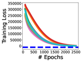
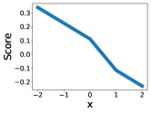
Refer to caption
Refer to caption
Refer to caption
Figure 7: Simulation results for score matching tasks with two-layer ReLU neural network (Uniform data). The left plot shows training loss where the dashed blue line indicates loss of convex score predictor (4). The middle plot shows score prediction by convex score predictor, which confirms our analysis in Section 3.3. The right plot shows sampling histogram via Langevin process with convex score predictor. Here the predicted score function is still close to score of Gaussian, which is due to the large weight decay, see Section 3.3 for details.

Figure 8,9, and 10 below show simulation results for score matching tasks with neural network of different types. In Figure 8, we show simulation results for neural network with absolute value activation and without skip connection. We use the same data samples and training parameters as explained in Section 5.1. The gap between non-convex training loss and convex score predictor loss can be due to the non-smoothness threshold function in the score matching training objective. The score prediction in the middle plot is aligned with our theoretic result in Section 3.3 and the sampling histogram in the right plot is consistent with the score prediction. In Figure 9 and 10, we set the weight decay parameter to β=b+1𝛽subscriptnorm𝑏1\beta=\|b\|_{\infty}+1.666See Section A.3 for definition of b𝑏b. Data samples and the rest training parameters are the same as in Section 5.1. Figure 9 shows results for two-layer ReLU network with skip connection and Figure 10 shows results for neural network with absolute value activation and with skip connection. Interestingly, the gap between non-convex training loss and convex score predictor loss is minor compared to Figure 8. The predicted score functions are linear with slope close to minus one over sample variance and interception close to sample mean, i.e., 11-1 and 00 respectively. This is aligned with our theoretic result in Appendix A.6.2 and A.6.3. The sampling histograms are consistent with the score prediction.
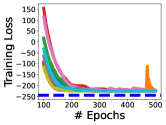
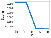
Refer to caption
Refer to caption
Refer to caption
Figure 8: Simulation results for score matching tasks with two-layer neural network with absolute value activation and no skip connection. The left plot shows training loss where the dashed blue line indicates loss of convex score predictor (14). The middle plot shows score prediction from convex score predictor, which confirms our analysis in Section 3.3. The right plot shows sampling histogram via Langevin process with convex score predictor. The ground truth distribution is standard Gaussian.
Refer to caption
Refer to caption
Refer to caption
Figure 9: Simulation results for score matching tasks with two-layer ReLU neural network with skip connection. The left plot shows training loss where the dashed blue line indicates loss of convex score predictor (18). The middle plot shows score prediction from convex score predictor, which confirms our analysis in Appendix A.6.2. The right plot shows sampling histogram via Langevin process with convex score predictor. The ground truth distribution is standard Gaussian.
Refer to caption
Refer to caption
Refer to caption
Figure 10: Simulation results for score matching tasks with two-layer neural network with absolute value activation and skip connection. The left plot shows training loss where the dashed blue line indicates loss of convex score predictor (20). The middle plot shows score prediction from convex score predictor, which confirms our analysis in Appendix A.6.3. The right plot shows sampling histogram via Langevin process with convex score predictor. The ground truth distribution is standard Gaussian.

C.2 Denoising Score Matching Simulations

In annealed Langevin sampling procedure, sθisubscript𝑠𝜃𝑖s_{\theta i} for i=1,2,,L𝑖12𝐿i=1,2,\ldots,L are neural networks trained for denoising score matching with different noise scales. Specifically, we take L=10,T=10,ϵ0=2e5,[σ1,,σL]formulae-sequence𝐿10formulae-sequence𝑇10subscriptitalic-ϵ02𝑒5subscript𝜎1subscript𝜎𝐿L=10,T=10,\epsilon_{0}=2e-5,[\sigma_{1},\ldots,\sigma_{L}] being the uniform grid from 111 to 0.010.010.01, and μ0subscript𝜇0\mu_{0} being uniform distribution from 11-1 to 111. Figure 11,12, and 13 below show simulation results for denoising score matching tasks for neural network of different types. We use the same simulation parameters as described in Section 5. The upper left plots in these three figures show the training loss where the dashed blue line is the objective value obtained by convex score predictors. The gap between non-convex training loss and convex score predictor loss indicates that our convex program solves the training problem globally. The first histograms in these three figures show sampling histograms via annealed Langevin process with convex score estimator. Since the ground truth distribution is standard Gaussian, our convex programs recover the ground truth data distribution. The rest histograms in these three figures are sampling results with non-convex score predictors corresponding to different learning rates, as what can be observed, the result relies heavily on learning rate choices and thus may not be stable.
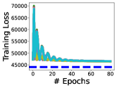
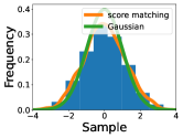
Refer to caption
Refer to caption
Refer to caption
Refer to caption
Refer to caption
Figure 11: Simulation results for denoising score matching tasks with neural network with absolute value activation and no skip connection. The upper left plot shows training loss where the dashed blue line indicates loss of convex score predictor (32). The second plot shows sampling histogram via annealed Langevin process with convex score predictor. The third, fourth, fifth plots show sampling histograms via annealed Langevin process with non-convex score predictors trained with learning rates 1,1e2,1e611𝑒21𝑒61,1e-2,1e-6 respectively. The ground truth distribution is standard Gaussian, which is recovered by our model.
Refer to caption
Refer to caption
Refer to caption
Refer to caption
Refer to caption
Figure 12: Simulation results for denoising score matching tasks with neural network with ReLU activation and skip connection. The upper left plot shows training loss where the dashed blue line indicates loss of convex score predictor (34). The second plot shows sampling histogram via annealed Langevin process with convex score predictor. The third, fourth, fifth plots show sampling histograms via annealed Langevin process with non-convex score predictors trained with learning rates 1,1e2,1e611𝑒21𝑒61,1e-2,1e-6 respectively. The ground truth distribution is standard Gaussian, which is recovered by our model.
Refer to caption
Refer to caption
Refer to caption
Refer to caption
Refer to caption
Figure 13: Simulation results for denoising score matching tasks with neural network with absolute value activation and skip connection. The upper left plot shows training loss where the dashed blue line indicates loss of convex score predictor (36). The second plot shows sampling histogram via annealed Langevin process with convex score predictor. The third, fourth, fifth plots show sampling histograms via annealed Langevin process with non-convex score predictors trained with learning rates 1,1e2,1e611𝑒21𝑒61,1e-2,1e-6 respectively. The ground truth distribution is standard Gaussian, which is recovered by our model.