Precedence-Constrained Winter Value for Effective Graph Data Valuation
Abstract
Data valuation is essential for quantifying data’s worth, aiding in assessing data quality and determining fair compensation. While existing data valuation methods have proven effective in evaluating the value of Euclidean data, they face limitations when applied to the increasingly popular graph-structured data. Particularly, graph data valuation introduces unique challenges, primarily stemming from the intricate dependencies among nodes and the exponential growth in value estimation costs. To address the challenging problem of graph data valuation, we put forth an innovative solution, Precedence-Constrained Winter (PC-Winter) Value, to account for the complex graph structure. Furthermore, we develop a variety of strategies to address the computational challenges and enable efficient approximation of PC-Winter. Extensive experiments demonstrate the effectiveness of PC-Winter across diverse datasets and tasks.
1 Introduction
The recent remarkable advancements in machine learning owe much of their success to the abundance of training data sources (Zhou et al., 2017). However, as models and the requisite training data continue to expand in scale, a disconnection often arises between the processes of data collection and model development. This disconnection raises crucial questions that demand our attention (Pei, 2020; Sim et al., 2022): (1) For data collectors, how can we ensure equitable compensation for individuals or organizations contributing to data collection? (2) For model developers, what strategies should they employ to identify and acquire the most relevant data that will maximize the performance of their models? In this context, the concept of data valuation has emerged as a pivotal area, aiming to quantify the inherent value of data measurably. Notable techniques in this field include Data Shapley (Ghorbani & Zou, 2019) and its successors (Kwon & Zou, 2021; Wang & Jia, 2023; Schoch et al., 2022), which have gained prominence in assessing the value of individual data samples. Despite the promise of these methods, they are primarily designed for Euclidean data, where samples are often assumed to be independent and identically distributed (i.i.d.). Given the prevalence of graph-structured data in the real world (Fan et al., 2019; Shahsavari & Abbeel, 2015; Li et al., ), there arises a compelling need to perform data valuation for graphs. However, due to the interconnected nature of samples (nodes) on graphs, existing data valuation frameworks are not directly applicable to addressing the graph data valuation problem.
In particular, designing data valuation methods for graph-structured data faces several fundamental challenges: Challenge I: Graph machine learning algorithms such as Graph Neural Networks (GNNs) (Kipf & Welling, 2016; Veličković et al., 2017; Wu et al., 2019) often involve both labeled and unlabeled nodes in their model training process. Therefore, unlabeled nodes, despite their absence of explicit labels, also hold intrinsic value. Existing data valuation methods, which typically assess a data point’s value based on its features and associated label, do not readily accommodate the valuation of unlabeled nodes within graphs. Challenge II: Nodes in a graph contribute to model performance in an interdependent and complex way: (1) Unlabeled nodes, while not providing direct supervision, can contribute to model performance by potentially affecting multiple labeled nodes through message-passing. (2) Labeled nodes, on the other hand, contribute by providing direct supervision signals for model training, and similarly to unlabeled nodes, they also contribute by affecting other labeled nodes through message-passing. Challenge III: Traditional data valuation methods are often computationally expensive due to repeated retraining of models (Ghorbani & Zou, 2019). The challenge is magnified in the context of graph-structured data, where samples contribute to model performance in multifaceted manners. Additionally, the inherent message-passing mechanism in GNN models further amplifies the computational demands for model re-training.
In this work, we make the first attempt to explore the challenging graph data valuation problem, to the best of our knowledge. In light of the aforementioned challenges, we propose the Precedence-Constrained Winter (PC-Winter) framework, a pioneering approach designed to intricately unravel and analyze the contributions of nodes within graph structures, thereby offering a detailed perspective on the valuation of graph elements. Our key contributions are as follows:
-
•
We formulate the graph data valuation problem as a unique cooperative game (Von Neumann & Morgenstern, 2007) with special coalition structures. Specifically, we decompose each node in the graph into several “players” within the game, each representing a distinct contribution to model performance. We then devise the PC-Winter to address the game, enabling the accurate valuation of all players. The PC-Winter values of these players can be conveniently combined to generate values for nodes and edges in the original graph.
-
•
We develop a comprehensive set of strategies to tackle the computational challenges, facilitating an efficient approximation of PC-Winter values.
-
•
Extensive experiments have validated the effectiveness of PC-Winter across various datasets and tasks. Furthermore, we execute detailed ablation studies and parameter analyses to deepen our insights into PC-Winter.
2 Preliminary and Related Work
In this section, we delve into some fundamental concepts that are essential for developing our methodology. More extensive literature exploration can be found in Appendix A.
2.1 Cooperative Game Theory
Cooperative game theory explores the dynamics where players, or decision-makers, can form alliances, known as coalitions, to achieve collectively beneficial outcomes (Branzei et al., 2008; Curiel, 2013). The critical components of such a game include a player set consisting of all players in the game and a utility function , which quantifies the value or payoff that each coalition of players can attain. Shapley Value (Shapley et al., 1953) is developed to fairly and efficiently distribute payoffs (values) among players.
Shapley value. The Shapley value for a player can be defined on permutations of as follows.
| (1) |
where denotes the set of all possible permutations of with denoting its cardinal number, and is predecessor set of , i.e, the set of players that appear before player in a permutation :
| (2) |
The Shapley value considers each player’s contribution to every possible coalition they could be a part of. Specifically, in Eq. (1), for each permutation , the marginal contribution of player is calculated as the difference in the utility function when player is added to an existing coalition . The Shapley value for is the average of these marginal contributions across all permutations in .
Winter Value. The Shapley value is to address cooperative games, where players collaborate freely and contribute on an equal footing. However, in many practical situations, cooperative games exhibit a Level Coalition Structure (Niyato et al., 2011; Vasconcelos et al., 2020; Yuan et al., 2016), reflecting a hierarchical organization. For instance, consider a corporate setting where different tiers of management and staff contribute to a project in varying capacities and with differing degrees of decision-making authority. Players within such a game are hierarchically categorized into nested coalitions with several levels, as depicted in Figure 1.
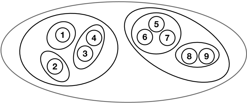
The outermost and largest ellipse represents the entire coalition and each of the smaller ellipse within the largest ellipse symbolizes a “sub-coaliation” at various hierarchical levels. Collaborations originate within the smallest sub-coalitions at the base level (illustrated by the innermost ellipses in Figure 1). These base units are then integrated into the next level, facilitating inter-coalition collaboration and enabling contributions to ascend to higher levels. This bottom-up flow of contributions continues, with each layer consolidating and passing on inputs to the next, culminating in a multi-leveled collaborative contribution to the final objective of the entire coalition. To accommodate such complex Level Coalition Structure, Winter value (Winter, 1989) was introduced. Winter value follows a similar permutation-based definition as Shapley Value (Eq. (1)) but with only a specific subset of permutations that respect the Level Coalition Structure. In these permutations, members of the same sub-coalition, regardless of the level, must appear in an unbroken sequence without interruptions. This ensures that the value attributed to each player is consistent with the level structure of the coalition. A formal and more comprehensive description of the Winter value, including its mathematical formulation, can be found in Appendix B.
2.2 Data Valuation and Data Shapley
Data valuation, increasingly popular with the rise of machine learning, quantifies the contribution of data points for machine learning tasks. The seminal work by Ghorbani & Zou (2019) introduces Data Shapley, applying cooperative game theory to data valuation. In this framework, training samples are the players , and the utility function assesses a model’s performance on subsets of these players using a validation set. With and , data values can be calculated with Eq. (1). However, Data Shapley and subsequent methods (Ghorbani & Zou, 2019; Kwon & Zou, 2021; Wang & Jia, 2022) primarily address i.i.d. data, overlooking potential coalitions or dependencies among data points.
2.3 Graphs and Graph Neural Networks
Consider a graph where denotes the set of nodes and denotes the set of edges. Each node carries a feature vector , where is the dimensionality of the feature space. Additionally, each node is associated with a label from a set of possible labels . We assume that only a subset are with known labels.
Graph Neural Networks (GNNs) (Kipf & Welling, 2016; Veličković et al., 2017; Wu et al., 2019) are prominent models for node classification on graphs. Specifically, from a local perspective for node , the -th GNN layer generally performs a feature averaging process as , where is the parameter matrix, and denote the degree and neighbors of node , respectively. After a total of layers, are utilized as the learned representation of . Such a feature aggregation process can be also described with a -level computation tree (Jegelka, 2022) rooted on node .
Definition 1 (Computation Tree).
For a node , its -level computation tree corresponding to a -layer GNN model is denoted as with as its root node. The first level of the tree consists of the immediate neighbors of , and each subsequent level is formed by the neighbors of nodes in the level directly above. This pattern of branching out continues, expanding through successive levels of neighboring nodes until the depth of the tree grows to .
The feature aggregation process in a -layer GNN model can be regarded as a bottom-up feature propagation process in the computation tree, where nodes in the lowest level are associated with their initial features. Therefore, the final representation of a node is affected by all nodes within its -hop neighborhood, which is referred to as the receptive field of node . The GNN model is trained using the (, ) pairs, where each labeled node in is represented by its final representation and corresponding label. Thus, in addition to labeled nodes, those unlabeled nodes that are within the receptive field of labeled nods also contribute to model performance.
3 Methodology
In classic machine learning models designed for Euclidean data, such as images and texts, training samples are typically assumed as i.i.d. Thus, each labeled sample contributes to the model performance by directly providing supervision signals through the training objective. However, due to the interdependent nature of graph data, nodes in a graph contribute to GNN performance in a more complicated way, which poses unique challenges. Specifically, as discussed in Section 2.3, both labeled and unlabeled nodes are involved in the training stage through the feature aggregation process and thus contribute to GNN performance. Next, we discuss how these nodes contribute to GNN performance.
Observation 1.
Unlabeled nodes influence GNN performance by affecting the final representation of labeled nodes. On the other hand, labeled nodes can contribute to GNN performance in two ways: (1) they provide direct supervision signals to GNN with their labels, and (2) just like unlabeled nodes, they can impact the final representation of other labeled nodes through feature aggregation. Note that both labeled nodes and unlabeled nodes can affect the final representations of multiple labeled nodes, as long as they lie within the receptive field of these labeled nodes. Hence, a single node can make multifaceted and heterogeneous contributions to GNN performance by affecting multiple labeled nodes in various manners.
3.1 The Graph Data Valuation Problem
Based on Observation 1, due to the heterogeneous and diverse effects of labeled and unlabeled nodes, it is necessary to perform fine-grained data valuation on graph data elements. In particular, we propose to decompose a node into distinct “duplicates” corresponding to their impact on different labeled nodes. We then aim to obtain values for all “duplicates” of these nodes. This could clearly express and separate how nodes impact GNN performance in various aspects. Following existing literature (Ghorbani & Zou, 2019; Wang & Jia, 2023; Yan & Procaccia, 2021), we approach the graph data value problem through a cooperative game. Next, we introduce the player set and the utility function of this game. In general, we define the graph data valuation game based on -layer GNN models.
Definition 2 (Player Set).
The player set in a graph data valuation game is defined as the union of nodes in the computation trees of labeled nodes. Duplication of nodes may occur within a single computation tree or across different labeled nodes’ computation trees. In the graph data valuation game, these potential duplicates are treated as distinct players, uniquely identified by their paths to the corresponding labeled node. We define the player set as the set of all these distinct players across the computation trees of all labeled nodes in .
Definition 3 (Utility Function).
Given a subset , we first generate a node-induced graph using their corresponding edges in the computation trees. Then, a GNN model is trained on the induced graph . Its performance is evaluated on a held-out validation set to serve as the utility of , calculated as , where measures the accuracy of the trained GNN model on a held-out validation set.
The goal of the graph data valuation problem is to assign a value to all players in with the help of the utility function . When calculated properly, these values are supposed to provide a detailed understanding of how players in contribute to the GNN performance in a fine-grained manner. Furthermore, these values can be flexibly combined to generate higher-level values for nodes and edges, which will be discussed in Section 3.5.
3.2 Precedence-Constrained Winter Value
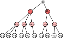
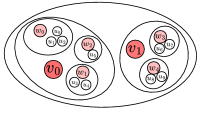
As discussed in Section 2.3, the final representations of a labeled node come from the hierarchical collaboration of all players in the computation tree . These labeled nodes with the updated representations then contribute to the GNN performance through the training objective. Such a contribution process forms a hierarchical collaboration between the players in , which can be illustrated with a contribution tree as shown in Figure 2a. In particular, the contribution tree is constructed by linking the root nodes of the computation trees of all labeled nodes with a dummy node representing the GNN training objective . In Figure 2a, for the ease of illustration, we set , include only labeled nodes, i.e, , and utilize , to denote the nodes in the lower level. The subtree rooted at a labeled node is the corresponding computation tree .
With the contribution tree, we observe the following about the coalition structure of the graph data valuation game.
Observation 2 (Level Coalition Structure).
As shown in Figure 2a, the players in hierarchically collaborate to contribute to the GNN performance. At the bottom level, the players are naturally grouped by their parents. Specifically, players with a common parent such as with their parent , establish a foundation sub-coalition. This sub-coalition is clearly depicted in Figure 2b. Moving up the tree, these parent nodes, like , serve as “delegates” for their respective sub-coalitions, further engaging in collaborations with other sub-coalitions. This interaction forms higher-level sub-coalitions, such as the one between , , , and in Figure 2b, indicating inter-coalition cooperation. This ascending process of coalition formation continues until the root node is reached, which represents the objective of the entire coalition consisting of all players. The depicted hierarchical collaboration process aligns with the Level Coalition Structure discussed in Section 2.1.
While the contribution tree shares similarities with the Level Coalition Structure illustrated in Section 2.1, a pivotal distinction lies in the representation and function of “delegates” (highlighted in red in Figure 2b) within each coalition. In the traditional Level Coalition Structure, contributions within a sub-coalition are made collectively, with each player or lower-level sub-coalition participating on an equitable basis. In contrast, the contribution tree framework distinguishes itself by designating a “delegate” within each sub-coalition, a player that represents and advances the collective contributions, establishing a directed and tiered flow of influence, hence forming a Unilateral Dependency Structure.
Observation 3 (Unilateral Dependency Structure).
In the contribution tree framework, a player contributes to the final objective through a hierarchical pathway facilitated by its ancestors (its “delegates” at different levels). Therefore, the collaboration between players in exhibits a Unilateral Dependency Structure, where a player ’s contribution is dependent on its ancestors.
According to these two observations, the players demonstrate unique coalition structures in the graph data valuation game. We aim to propose a permutation-based valuation framework similar to Eq. (1) to address the cooperative game with both Level Coalition Structure and Unilateral Dependency Structure. In particular, instead of utilizing all the permutations as in Eq. (1), only the permissible permutations aligning with such coalition structures are included in the value calculations. As we described in Section 2.1, cooperative games with Level Coalition Structure have been addressed by the Winter value (Winter, 1989; Chantreuil, 2001). Specifically, a permutation respecting the Level Coalition Structure must ensure that players in the same (sub-)coalition, regardless of its level, are grouped together without interruption from other players (Winter, 1989). In our scenario, any subtree of the contribution tree corresponds to a sub-coalition as demonstrated in Figure 2. Hence, we need to ensure that for any player , the player and its descendants in the contribution tree should be grouped together in the permutation. For example, the players should present together as a group in the permutation with potentially different orders. On the other hand, to ensure the Unilateral Dependency Structure, a permutation must maintain a partial order. Specifically, for any player in the permutation, its descendants must present in later positions in the permutation than . Otherwise, the descendants of cannot make non-trivial contributions, resulting in marginal contributions.
We formally define the permissible permutations that align with both Level Coalition Structure and Unilateral Dependency Structure utilizing the following two constraints.
Constraint 1 (Level Constraint).
For any player , the set of its descendants in the contribution tree is denoted as . Then, a permutation aligning with the Level Coalition Structure satisfies the following Level Constraint.
where denotes the positional rank of the in .
Constraint 2 (Precedence Constraint).
A permutation aligning with the Unilateral Dependency Structure satisfies the following Precedence Constraint:
We denote the set of permissible permutations satisfying both Level Constraint and Precedence Constraint as . Then, we define the Precedence-Constrained Winter (PC-Winter) value for a player with the permutations in as follows.
| (3) |
where is the utility function (see Definition 3), and denotes the predecessor set of in as defined in Eq. (2).
3.3 Permissible Permutations for PC-Winter
To calculate PC-Winter value, it is required to obtain all permissible permutations. A straightforward approach is to enumerate all permutations, verify their validity, and only retain the permissible permutations. However, such an approach is computationally intensive and typically not feasible as the number of permutations grows exponentially as the number of players increases. In this section, to address this challenge, we propose a novel method to directly generate these permutations by traversing the contribution tree with Depth-First Search (DFS). Specifically, each DFS traversal results in a preordering, which is a list of the nodes (players) in the order that they were visited by DFS. Such a preordering naturally defines a permutation of by simply removing the dummy node in the contribution tree from the preordering. By iterating all possible DFS traversals of the contribution tree, we can obtain all permutations in , which is demonstrated in the following theorems.
Theorem 1 (Specificity).
Given a contribution tree with a set of players , any DFS traversal over the results in a permissible permutation of that satisfies both the Level Constraint and Precedence Constraint.
Theorem 2 (Exhaustiveness).
Given a contribution tree with a set of players , any permissible permutation can be generated by a corresponding DFS traversal of .
The proofs for these two theorems can be found in Section C in the Appendix. Theorem 1 demonstrates that DFS traversals always specifically generate permissible permutations. On the other hand, Theorem 2 ensures the exhaustiveness of generation, which allows us to obtain all permutations in by DFS traversal. Together, these two theorems ensure us to exactly generate the set of permissible permutations .
Notably, the calculation of PC-Winter value involves two steps: 1) generating with DFS traversals; and 2) calculating the PC-Winter value according to Eq. (3). Nonetheless, it can be done in a streaming way while we perform the DFS traversals. Specifically, once we reach a player in a DFS traversal, we can immediately calculate its marginal contribution. The PC-Winter values for all players are computed by averaging their marginal contributions calculated from all possible DFS traversals.
3.4 Efficient Approximation of PC-Winter
Calculating the PC-Winter value for players in is infeasible due to computational intensity, arising from: 1) The exponential growth in the number of permissible permutations with more players, rendering exhaustive enumeration intractable; 2) The necessity to re-train the GNN within the utility function for each permutation, a process repeated times to account for every player’s marginal contribution; and 3) The intensive computation involved in GNN re-training, requiring feature aggregation over the graph that increases in complexity with the graph’s size. These challenges necessitate an efficient approximation method for PC-Winter valuation in practical applications. We propose three strategies to address these computational issues.
Permutation Sampling. Following Data Shapley (Ghorbani & Zou, 2019), we adopt Monte Carlo (MC) sampling to randomly sample a subset of permissible permutations denoted as . Then, we utilize to replace in Eq. (3) for approximating PC-Winter value.
Hierarchical Truncation. GNN models often demonstrate a phenomenon of neighborhood saturation, i.e, these models achieve satisfactory performance even when trained on a subgraph using only a small subset of neighbors, rather than the full neighborhood (Hamilton et al., 2017; Liu et al., 2021; Ying et al., 2018; Chen et al., 2017), indicating diminishing returns from additional neighbors beyond a certain point. This indicates that for a player in a permissible permutation generated by DFS over the contribution tree, the marginal contributions of its late visited child players are insignificant. Thus, we propose hierarchical truncation for efficiently obtaining the marginal contributions by directly approximating insignificant values as . Specifically, during the DFS traversal, given a truncation ratio , we only compute actual marginal contributions for players in the first portion of each node’s child subtrees, approximating the marginal contributions of players in the remaining subtrees as . For example, in Figure 2a, given a truncation ratio , when DFS reaches player , we only calculate marginal contributions for players in the subtree rooted at . Furthermore, in the subtree rooted at , due to the hierarchical truncation process, only the marginal contribution of is evaluated, those for node and are directly set to . This approach is further optimized by adjusting truncation ratios based on the tree level, accommodating varying contribution patterns across levels. In particular, we organize the pair of truncation ratio as -, indicating we truncate (or ) portion of subtrees (or child players) of (or ). We show how the hierarchical truncation helps tremendously reduce the required model re-training in Appendix D.
Local Propagation. To enhance scalability, we leverage SGC (Wu et al., 2019) in our utility function, which simplifies GNNs by aggregating node features before applying an MLP. According to the Level Constraint (Constraint 1), the players within the same computation tree are grouped together in the permutation. Therefore, the induced graph of any coalition defined by a permissible permutation consists of a set of separated computation trees (or a partial computation tree corresponding to the last visited labeled node in ). A key observation is that the feature aggregation process for the labeled nodes can be done independently within their own computation trees. Hence, instead of performing the feature propagation for the entire induced graph, we propose to perform local propagation only on necessary computation trees. In particular, the aggregated representation for a labeled node is fixed after we traverse its entire computation tree in DFS. Therefore, for evaluating a player ’s marginal contribution, only the partial computation tree of the last visited labeled node requires local propagation, minimizing feature propagation efforts.
The PC-Winter values for all players are approximated with these three strategies in a streaming manner. In particular, we randomly traverse the contribution tree with DFS for times. During each DFS traversal, the marginal contributions for all players in are efficiently obtained with the help of hierarchical truncation and local propagation strategies. The marginal contributions calculated through these DFS traversals are averaged to approximate the PC-Winter value for all players.
3.5 From PC-Winter to Node and Edge Values
The PC-Winter values for players in can be flexibly combined to obtain the values for elements in the original graph, which are illustrated in this section. Specifically, as discussed in Section 3.1, multiple “duplicates” of a node in the original graph may potentially present in . Thus, we could obtain node value for the node by summing the PC-Winter values of all its “duplicates” in . On the other hand, each player (except for the rooted labeled players) in corresponds to an “edge” in the contribution tree as identified by the player and its parent. For instance, in Figure 2a, the player corresponds to “edge” connecting and . Therefore, DFS traversals also generate permutations for these “edges”. From this perspective, the marginal contribution for a player calculated through a DFS traversal can be also regarded as the marginal contribution of its corresponding edge, if we treat this process as gradually adding “edges” to connecting the players in . Hence, the PC-Winter values for players in can be regarded as PC-Winter values for their corresponding “edges” in the contribution tree. Multiple “duplicates” of an edge in the original graph may be present in the contribution tree. Hence, similar to the node values, we define the edge value for by taking the summation of the PC-Winter value for all its “duplicates” in the contribution tree.
4 Experiment
4.1 Overall Experimental Setup
Datasets. We assess the proposed approach on six real-world benchmark datasets: Cora, Citeseer, and Pubmed (Sen et al., 2008), Amazon-Photo, Amazon-Computer, and Coauther-Physics (Shchur et al., 2018). The detailed statistics of datasets are summarized in Table 2 in Appendix G.
Settings. Our experiments focus on the inductive setting, which aims to generalize a trained model to unseen nodes or graphs and is commonly adopted in real-world graph applications (Hamilton et al., 2017; Van Belle et al., 2022; Jendal et al., 2022; D’Amico et al., 2023). Unlike the transductive setting (Kipf & Welling, 2016) which incorporates the test nodes in the model training process, the inductive setting separates them apart from the training graph. Such a separation allows us to measure the value of the graph elements in the training graph solely based on their contribution to GNN model training. Following (Hamilton et al., 2017), we split each graph into disjoint subgraphs: training graph , validation graph , and test graph . More details on the splitting can be found in Appendix G.2. Throughout the experiments, we focus on -layer GNN models for both approximating and evaluating the PC-Winter values. To obtain the PC-Winter values, we run permutations in a streaming way as described in Section 3.4. This process terminates with a convergence criterion as detailed in Appendix G.3. PC-Winter typically terminates with a different number of permutations for different datasets. The other hyper-parameters including the truncation ratios are also detailed in Appendix G.4.
4.2 Dropping High-Value Nodes
In this section, we aim to evaluate the quality of data values produced by PC-Winter via dropping high-value nodes from the graph. Dropping high-value nodes is expected to significantly diminish performance, and thus the performance observed after removing high-value nodes serves as a strong indicator of the efficacy of graph data valuation. Notably, the node values are calculated from PC-Winter values as described in Section 3.5.
To demonstrate the effectiveness of PC-Winter, we include Random value, Degree value, Leave-one-out (LOO) value, and Data Shapley value as baselines. A more detailed description of these baselines is included in Section G.5 in the Appendix. Notably, there is a recent work (Chen et al., 2022) that aims at characterizing the impact of elements on model performance. Their goal is to approximate LOO value. Thus, we do not include it as a baseline as LOO is already included.
To conduct node-dropping experiments, nodes are ranked by their assessed values for each method and removed sequentially from the training graph . After each removal, we train a GNN model based on the remaining graph and evaluate its performance on . Performance changes are depicted through a curve that tracks the model’s accuracy as nodes are progressively eliminated.
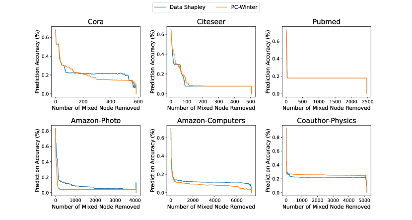
Labeled nodes often contribute more significantly to model performance than unlabeled nodes because they directly offer supervision. Therefore, it is logical that, with accurately assigned node values, labeled nodes should be prioritized for removal over unlabeled nodes. We empirically validate this hypothesis in Figure 8, discussed in Section E of the Appendix. Specifically, in nearly all datasets, our observations reveal that the majority of labeled nodes are removed prior to the unlabeled nodes by both PC-Winter and Data Shapley. This leads to a noticeable plateau in the latter portion of the performance curves since a GNN model cannot be effectively trained with only unlabeled nodes. Consequently, this scenario significantly hampers the ability to assess the value of unlabeled nodes. Therefore, we propose to conduct separate assessments for the values of labeled and unlabeled nodes. In this section, we only inlcude the results for unlabeled nodes, while the results for labeled nodes are presented in Appendix F.
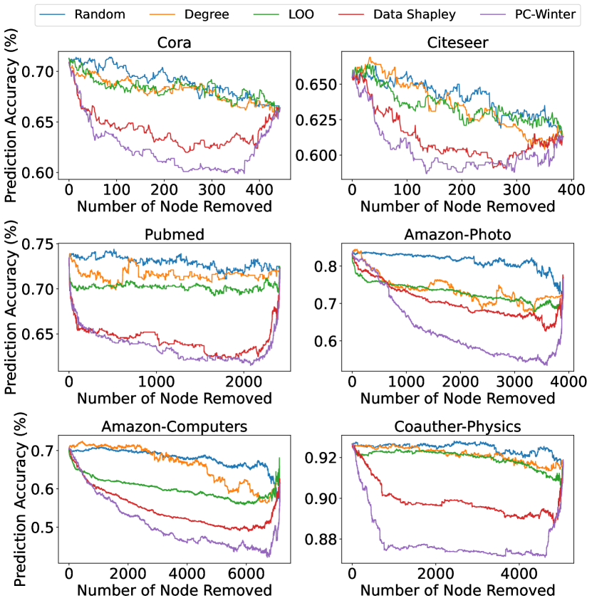
Results and Analysis. Figure 3 illustrates the performance comparison between PC-Winter and other baselines across various datasets. From Figure 3, we make the following observations. First, the removal of high-value unlabeled nodes identified by PC-Winter consistently results in the most significant decline in model performance across various datasets. This is particularly evident after removing a relatively small fraction (10%-20%) of the highest-value nodes. This trend underscores the critical importance of these high-value nodes. Notably, in most datasets PC-Winter outperforms the best baseline method, Data Shapley, by a considerable margin, highlighting its effectiveness. Second, the decrease in performance caused by our method is not only substantial but also persistent throughout the node-dropping process, further validating the effectiveness of PC-Winter. Third, the performance curves of PC-Winter and Data Shapley eventually rebound towards the end. This rebound corresponds to the removal of unlabeled nodes that make negative contributions. Their removal aids in improving performance, ultimately reaching the performance of an MLP when all nodes are excluded. This upswing not only evidences the discernment of PC-Winter and Data Shapley in ascertaining node values but also showcases the particularly acute precision of PC-Winter. These insights collectively affirm the capability of PC-Winter in accurately assessing node values.
4.3 Adding High-Value Edges
In this section, we explore the impact of adding high-value elements to a graph, providing an alternative perspective to validate the effectiveness of data valuation. Notably, adding high-value nodes to a graph typically involves the concurrent addition of edges, which complicates the addition process. Thus, we target the addition of high-value edges, providing a complementary perspective to our data valuation analysis. As previously described in Section 3.5, the flexibility of PC-Winter allows for obtaining edge values without a separate “reevaluation” process for edges. In edge addition, we keep all nodes in and sequentially add edges according to the edge values in descending order, starting with the highest-valued ones. Similar to the node-dropping experiments, the effectiveness of the edge addition is demonstrated through performance curves. We include Random value, Edge-Betweeness, Leave-one-out (LOO) as baselines. Notably, here, Random and LOO specifically pertain to edges, and while we use the same terminology as in the prior section, they are distinct methods, which are detailed in Section G.5 of the Appendix.
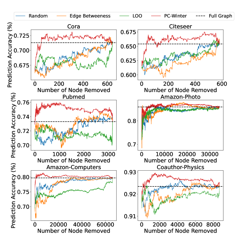
Results and Analysis. Figure 4 illustrates that the Random, LOO, and Edge-Betweeness baselines achieve only linear performance improvements with the addition of more edges, failing to discern the most impactful ones for a sparse yet informative graph. In contrast, the inclusion of edges based on the PC-Winter value results in a steep performance climb, affirming the PC-Winter’s efficacy in pinpointing key edges. Notably, the Cora dataset reaches full-graph performance using merely 8% of the edges selected by PC-Winter. Moreover, with just 10% of PC-Winter-selected edges, the accuracy climbs to 72.9%, outperforming the full graph’s 71.3%, underscoring PC-Winter’s capability to identify valuable edges. This trend is generally consistent across other datasets as well.
4.4 Ablation Study, Parameter and Efficiency Analysis
In this section, we conduct an ablation study, parameter analysis, and efficiency analysis to gain deeper insights into PC-Winter. These analyses are done with node-dropping experiments. We only present the results of Cora and Amazon-Photo. The results of additional datasets are in Appendix H.
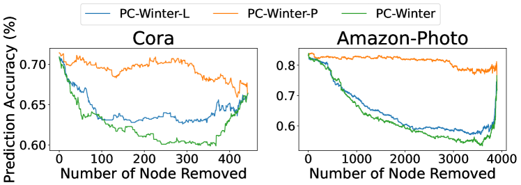
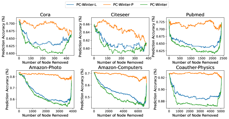
Ablation Study. We conduct an ablation study to understand how the two constraints in Section 3.2 affect the effectiveness of PC-Winter. We introduce two variants of PC-Winter by lifting one of the constraints for the permutations. In particular, we define PC-Winter-L using the permutations satisfying the Level Constraint. Similarly, PC-Winter-P is defined with permutations only satisfying Precedence Constraint. As shown in Figure 5, PC-Winter value outperforms the PC-Winter-L and PC-Winter-P on both datasets, which demonstrates that both constraints are crucial for PC-Winter.
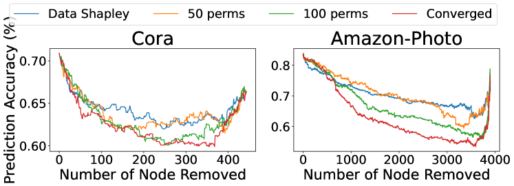
Impact of Permutation Number. We investigate how the number of permutations affects the effectiveness of PC-Winter. Note that PC-Winter converges on Cora and Amazon-Photo in and permutations, respectively. As shown in Figure 6, unsurprisingly, a larger number of permutations yield more accurate value estimations leading to a more significant performance drop. More importantly, even with a smaller number of permutations such as and , PC-Winter maintains comparable or superior performance to Data Shapley.
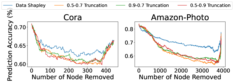
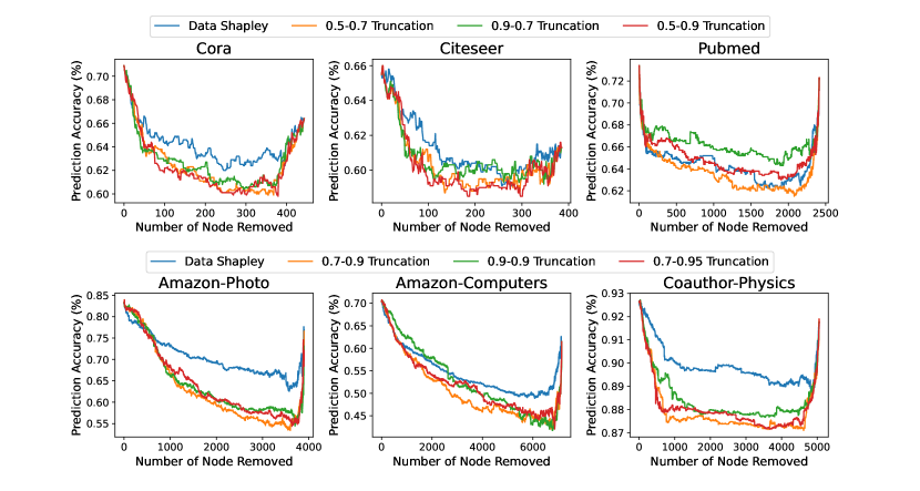
Impact of Truncation Ratios. We investigate how the truncation ratios in the hierarchical truncation strategy affect PC-Winter. We adopt different pairs of truncation ratios including , , and . Figure 7 demonstrates that PC-Winter tolerates heavy truncation ratios without significantly compromising performance, which would help further reduce computation time.
Efficiency Analysis. We conduct efficiency analysis for PC-Winter compared with Data Shapley. A detailed and comprehensive analysis, including permutation time comparison and running time comparison in terms of GPU hours on datasets, are available in Appendix H.4. This analysis highlights that PC-Winter is significantly more efficient than Data Shapley.
5 Conclusion
In this paper, we introduce PC-Winter, an innovative approach for effective graph data valuation. The method is specifically designed for graph-structured data and addresses the challenges posed by unlabeled elements and complex node dependencies within graphs. Furthermore, we introduce a set of strategies for reducing the computational cost, enabling efficient approximation of PC-Winter. Extensive experiments demonstrate the practicality and effectiveness of this PC-Winter in various datasets and tasks. Though PC-Winter is significantly more efficient than Data Shapley, its scalability is still limited. Hence, a promising and important future direction is to further improve its efficiency. Furthermore, PC-Winter is limited to homogeneous graphs. Extending PC-Winter to heterogeneous graphs is another potential future direction.
Ethics and Impact Statement
To the best of our knowledge, there are no ethical issues with this paper.
This work contributes to the growing field of Graph Machine Learning, which has applications in numerous domains such as social network analysis, recommendation systems, fraud detection, biological data analysis, etc. By focusing on the valuation of graph data, our work aids in understanding the relative importance of different parts of the graph and can guide the development of more sophisticated graph-based algorithms and models. This research can lead to advancements in the aforementioned areas and the potential for groundbreaking discoveries.
References
- Branzei et al. (2008) Branzei, R., Dimitrov, D., and Tijs, S. Models in cooperative game theory, volume 556. Springer Science & Business Media, 2008.
- Bruna et al. (2013) Bruna, J., Zaremba, W., Szlam, A., and LeCun, Y. Spectral networks and locally connected networks on graphs. arXiv preprint arXiv:1312.6203, 2013.
- Chantreuil (2001) Chantreuil, F. Axiomatics of level structure values. Power Indices and Coalition Formation, pp. 45–62, 2001.
- Chen et al. (2017) Chen, J., Zhu, J., and Song, L. Stochastic training of graph convolutional networks with variance reduction. arXiv preprint arXiv:1710.10568, 2017.
- Chen et al. (2022) Chen, Z., Li, P., Liu, H., and Hong, P. Characterizing the influence of graph elements. arXiv preprint arXiv:2210.07441, 2022.
- Curiel (2013) Curiel, I. Cooperative game theory and applications: cooperative games arising from combinatorial optimization problems, volume 16. Springer Science & Business Media, 2013.
- D’Amico et al. (2023) D’Amico, E., Muhammad, K., Tragos, E., Smyth, B., Hurley, N., and Lawlor, A. Item graph convolution collaborative filtering for inductive recommendations. In European Conference on Information Retrieval, pp. 249–263. Springer, 2023.
- Fan et al. (2019) Fan, W., Ma, Y., Yin, D., Wang, J., Tang, J., and Li, Q. Deep social collaborative filtering. In Proceedings of the 13th ACM RecSys, 2019.
- Gasteiger et al. (2018) Gasteiger, J., Bojchevski, A., and Günnemann, S. Predict then propagate: Graph neural networks meet personalized pagerank. arXiv preprint arXiv:1810.05997, 2018.
- Ghorbani & Zou (2019) Ghorbani, A. and Zou, J. Data shapley: Equitable valuation of data for machine learning. In International conference on machine learning, pp. 2242–2251. PMLR, 2019.
- Hamilton et al. (2017) Hamilton, W., Ying, Z., and Leskovec, J. Inductive representation learning on large graphs. Advances in neural information processing systems, 30, 2017.
- Jegelka (2022) Jegelka, S. Theory of graph neural networks: Representation and learning. arXiv preprint arXiv:2204.07697, 2022.
- Jendal et al. (2022) Jendal, T. E., Lissandrini, M., Dolog, P., and Hose, K. Simple and powerful architecture for inductive recommendation using knowledge graph convolutions. arXiv preprint arXiv:2209.04185, 2022.
- Jia et al. (2019) Jia, R., Dao, D., Wang, B., Hubis, F. A., Gurel, N. M., Li, B., Zhang, C., Spanos, C. J., and Song, D. Efficient task-specific data valuation for nearest neighbor algorithms. arXiv preprint arXiv:1908.08619, 2019.
- Just et al. (2023) Just, H. A., Kang, F., Wang, J. T., Zeng, Y., Ko, M., Jin, M., and Jia, R. Lava: Data valuation without pre-specified learning algorithms. arXiv preprint arXiv:2305.00054, 2023.
- Kipf & Welling (2016) Kipf, T. N. and Welling, M. Semi-supervised classification with graph convolutional networks. arXiv preprint arXiv:1609.02907, 2016.
- Kwon & Zou (2021) Kwon, Y. and Zou, J. Beta shapley: a unified and noise-reduced data valuation framework for machine learning. arXiv preprint arXiv:2110.14049, 2021.
- Kwon & Zou (2023) Kwon, Y. and Zou, J. Data-oob: Out-of-bag estimate as a simple and efficient data value. arXiv preprint arXiv:2304.07718, 2023.
- (19) Li, P., Wang, J., Qiao, Y., Chen, H., Yu, Y., Yao, X., Gao, P., Xie, G., and Song, S. An effective self-supervised framework for learning expressive molecular global representations to drug discovery. Briefings in Bioinformatics.
- Liu et al. (2021) Liu, X., Yan, M., Deng, L., Li, G., Ye, X., and Fan, D. Sampling methods for efficient training of graph convolutional networks: A survey. IEEE/CAA Journal of Automatica Sinica, 9(2):205–234, 2021.
- Niyato et al. (2011) Niyato, D., Vasilakos, A. V., and Kun, Z. Resource and revenue sharing with coalition formation of cloud providers: Game theoretic approach. In 2011 11th IEEE/ACM International Symposium on Cluster, Cloud and Grid Computing, pp. 215–224. IEEE, 2011.
- Nohyun et al. (2022) Nohyun, K., Choi, H., and Chung, H. W. Data valuation without training of a model. In The Eleventh International Conference on Learning Representations, 2022.
- Pei (2020) Pei, J. A survey on data pricing: from economics to data science. IEEE Transactions on knowledge and Data Engineering, 34(10):4586–4608, 2020.
- Schoch et al. (2022) Schoch, S., Xu, H., and Ji, Y. Cs-shapley: Class-wise shapley values for data valuation in classification. Advances in Neural Information Processing Systems, 35:34574–34585, 2022.
- Sen et al. (2008) Sen, P., Namata, G., Bilgic, M., Getoor, L., Galligher, B., and Eliassi-Rad, T. Collective classification in network data. AI magazine, 29(3):93–93, 2008.
- Shahsavari & Abbeel (2015) Shahsavari, B. and Abbeel, P. Short-term traffic forecasting: Modeling and learning spatio-temporal relations in transportation networks using graph neural networks. University of California at Berkeley, Technical Report No. UCB/EECS-2015-243, 2015.
- Shapley et al. (1953) Shapley, L. S. et al. A value for n-person games. 1953.
- Shchur et al. (2018) Shchur, O., Mumme, M., Bojchevski, A., and Günnemann, S. Pitfalls of graph neural network evaluation. arXiv preprint arXiv:1811.05868, 2018.
- Sim et al. (2022) Sim, R. H. L., Xu, X., and Low, B. K. H. Data valuation in machine learning:“ingredients”, strategies, and open challenges. In Proc. IJCAI, pp. 5607–5614, 2022.
- Van Belle et al. (2022) Van Belle, R., Van Damme, C., Tytgat, H., and De Weerdt, J. Inductive graph representation learning for fraud detection. Expert Systems with Applications, 193:116463, 2022.
- Vasconcelos et al. (2020) Vasconcelos, V. V., Hannam, P. M., Levin, S. A., and Pacheco, J. M. Coalition-structured governance improves cooperation to provide public goods. Scientific reports, 10(1):9194, 2020.
- Veličković et al. (2017) Veličković, P., Cucurull, G., Casanova, A., Romero, A., Lio, P., and Bengio, Y. Graph attention networks. arXiv preprint arXiv:1710.10903, 2017.
- Von Neumann & Morgenstern (2007) Von Neumann, J. and Morgenstern, O. Theory of games and economic behavior (60th Anniversary Commemorative Edition). Princeton university press, 2007.
- Wang & Jia (2023) Wang, J. T. and Jia, R. Data banzhaf: A robust data valuation framework for machine learning. In International Conference on Artificial Intelligence and Statistics, pp. 6388–6421. PMLR, 2023.
- Wang & Jia (2022) Wang, T. and Jia, R. Data banzhaf: A data valuation framework with maximal robustness to learning stochasticity. arXiv preprint arXiv:2205.15466, 2022.
- Winter (1989) Winter, E. A value for cooperative games with levels structure of cooperation. International Journal of Game Theory, 18:227–240, 1989.
- Wu et al. (2019) Wu, F., Souza, A., Zhang, T., Fifty, C., Yu, T., and Weinberger, K. Simplifying graph convolutional networks. In ICML. PMLR, 2019.
- Xu et al. (2018) Xu, K., Hu, W., Leskovec, J., and Jegelka, S. How powerful are graph neural networks? arXiv preprint arXiv:1810.00826, 2018.
- Yan & Procaccia (2021) Yan, T. and Procaccia, A. D. If you like shapley then you’ll love the core. In Proceedings of the AAAI Conference on Artificial Intelligence, volume 35, pp. 5751–5759, 2021.
- Ying et al. (2018) Ying, R., He, R., Chen, K., Eksombatchai, P., Hamilton, W. L., and Leskovec, J. Graph convolutional neural networks for web-scale recommender systems. In Proceedings of the 24th ACM SIGKDD international conference on knowledge discovery & data mining, pp. 974–983, 2018.
- Yoon et al. (2020) Yoon, J., Arik, S., and Pfister, T. Data valuation using reinforcement learning. In International Conference on Machine Learning, pp. 10842–10851. PMLR, 2020.
- Yuan et al. (2016) Yuan, P., Xiao, Y., Bi, G., and Zhang, L. Toward cooperation by carrier aggregation in heterogeneous networks: A hierarchical game approach. IEEE Transactions on Vehicular Technology, 66(2):1670–1683, 2016.
- Zhang et al. (2021) Zhang, S., Liu, Y., Sun, Y., and Shah, N. Graph-less neural networks: Teaching old mlps new tricks via distillation. arXiv preprint arXiv:2110.08727, 2021.
- Zhou et al. (2017) Zhou, L., Pan, S., Wang, J., and Vasilakos, A. V. Machine learning on big data: Opportunities and challenges. Neurocomputing, 237:350–361, 2017.
Appendix A Additional Related Work
This section presents an extended review of related works, offering a broader and more nuanced exploration of the literature surrounding Data Valuation and Graph Neural Networks.
A.1 Data Valuation
Data Shapley is proposed in (Ghorbani & Zou, 2019) which computes data values with Shapley values in cooperative game theory. Beta Shapley (Kwon & Zou, 2021) is a further generalization of Data Shapley by relaxing the efficiency axiom of the Shapley value. Data Banzhaf (Wang & Jia, 2022) offers a data valuation method which is robust to data noises. Data Valuation with Reinforcement Learning is also explored by (Yoon et al., 2020). KNN-Shapley (Jia et al., 2019) estimates the shapley Value for the K-Nearest Neighbours algorithm in linear time. CS-Shapley (Schoch et al., 2022) provides a new valuation method that differentiate in-class contribution and out-class contribution. Data-OOB (Kwon & Zou, 2023) proposes a data valuation method for a bagging model which leverages the out-of-bag estimate. Just, Hoang Anh, et al (Just et al., 2023) introduce a learning-agnostic data valuation framework by approximating the utility of a dataset according to its class-wise Wasserstein distance. Another training-free data valuation method utilizing the complexity-gap score is proposed at the same time (Nohyun et al., 2022). However, those methods are not designed for the evaluation of data value of graph data which bears higher complexity due to the interconnections of individual nodes.
A.2 Graph Neural Networks
Graph Neural Networks (GNNs) generate informative representations from graph-structured data and facilitate the solving of many graph-related tasks. Bruna et al. (Bruna et al., 2013) first apply the spectral convolution operation to graph-structured data. From the spatial perspective, the spectral convolution can be interpreted to combine the information from its neighbors. GCN (Kipf & Welling, 2016) simplified this spectral convolution and proposed to use first-order approximation. Since then, many other attention-based, sampling-based and simplified GNN variants which follow the same neighborhood aggregation design have been proposed (Veličković et al., 2017; Hamilton et al., 2017; Gasteiger et al., 2018; Wu et al., 2019).Theoretically, those Graph neural networks typically enhance node representations and model expressiveness through a message-passing mechanism, efficiently integrating graph data into the learning of representations (Xu et al., 2018).
Appendix B Mathematical Formulation of Winter Value
The Shapley value offers a solution for equitable payoff distribution in cooperative games, assuming that players cooperate without any predefined structure. In reality, however, cooperative games often have inherent hierarchical coalitions. To accommodate these structured coalitions, the Winter value extends Shapley value to handle this extra coalition constraints.
Specifically, considering level structures , with representing a sequence of player partitions. Here, a partition, , subdivides the player set into distinct, non-empty subsets. These subsets, , satisfy the condition that the union of all in reconstructs the original player set , which means for every , . This partition sequence forms a hierarchy where represents individual players as the leaves of the structure and functions as the root of this hierarchy.
We then determine , the set of all permissible permutations, starting with a single partition :
A permissible permutation from the set requires that players from any derived coalition of must appear consecutively. Given the defined set of permissible permutations , the Winter value for player is calculated as:
where is the set of predecessors of at the permutation and is the utility function in the cooperative game.
Appendix C Proofs of Theorems
Theorem 1 (Specificity).
Given a contribution tree with a set of players , any DFS traversal over the results in a permissible permutation of that satisfies both the Level Constraint and Precedence Constraint.
Proof.
We validate the theorem by demonstrating that a permutation obtained through pre-order traversal on meets Level Constraints and Precedence Constraints. (1) Level Constraints: During a pre-order traversal of , a node and its descendants are visited sequentially before moving to another subtree. Thus, in the resulting permutation , the positions of and any are inherently close to each other, satisfying the condition . This contiguous traversal ensures that all descendants and the node itself form a continuous sequence in , meeting the Level Constraint. (2) Precedence Constraints: In the same traversal, each node is visited before its descendants. Therefore, in , the position of always precedes the positions of its descendants, i.e., for all . This traversal pattern naturally embeds the hierarchy of the tree into the permutation, ensuring that ancestors are positioned before their descendants, in line with the Precedence Constraint. ∎
Theorem 2 (Exhaustiveness).
Given a contribution tree with a set of players , any permissible permutation can be generated by a corresponding DFS traversal of .
Proof.
To prove the theorem of exhaustiveness, consider a contribution tree with a set of players and any permissible permutation . We apply induction on the depth of . For the base case, when has a depth of 1, which is no dependencies among players, any permissible permutation of players is trivially generated by a DFS traversal since there are no constraints on the order of traversal. For the inductive step, assume the theorem holds for contribution trees of depth . For a contribution tree of depth , consider its root node and subtrees of depth rooted at the child nodes of the root node. For any given permissible permutation corresponding to the , according to the Level Constraint, it is a direct composition of the permissible permutations corresponding to the subtrees of depth rooted at the child nodes of the root node. Now we can construct a DFS traversal over the contribution tree that can generate . Specifically, the order of composition defines the traversal order of the child nodes of the root node. Furthermore, by the inductive hypothesis, any permissible permutations corresponding to the subtrees can be generated by DFS traversal over the subtrees. Hence, at each child node of the root node, we just follow the corresponding DFS traversal of its corresponding tree. This DFS traversal can generate the given permutation , which completes the proof. ∎
Appendix D Hierarchical Truncation
Dataset w.o. Truncation w.t. Truncation Cora 2241 756 Citeseer 1388 535 Pubmed 3683 887 Amazon-Photo 147664 6258 Amazon-Computer 317959 12139 Coauther-Physics 11178 852
In the Table 1, we present data comparing the number of model re-trainings on the all six dataset with and without the application of truncation. For the Citeseer dataset, the truncation ratios are defined as 1st-hop: 0.5 and 2nd-hop: 0.7. For the remaining datasets, the truncation ratios are set at 1st-hop: 0.7 and 2nd-hop: 0.9. The results clearly indicate that the number of model re-trainings is substantially reduced when truncation is applied. For instance, focusing on the Citeseer dataset the application of truncation significantly reduces the number of retrainings from 1388 to 535. This significant decrease, especially in larger datasets like Amazon-Photo and Amazon-Computer, where retraining instances decrease from 147664 to 6258 and from 317959 to 12139 respectively, can be attributed to the substantial number of 2-distance neighbors present in these datasets. The application of truncation effectively reduces the computation by omitting a considerable portion of these neighbors. This finding also implies that overall training time is decreased while still maintaining the ability to accurately measure the total marginal contribution.
Appendix E Mixed Node Dropping Experiment
As mentioned in the experiment part of paper, labeled nodes will dominate the performance curve when both labeled nodes and unlabeled nodes. The corresponding experiment result is shown in the Figure 8. This experiment validates the assumption that a effective data valuation method would naturally rank labeled nodes for earlier removal over their unlabeled counterparts. For instance, in the Cora dataset, we can observe that the initial drop in accuracy is significant, indicating the removal of high-value labeled nodes. As the experiment progresses and more nodes are removed, the accuracy barely changes, reflecting the removal of unlabeled nodes which has a minimal impact on performance when most labeled nodes are unavailable. The observed pattern across all datasets is consistent: there is a substantial drop in performance at the beginning, followed by a plateau with minimal changes. This suggests that the initial set of nodes removed, predominantly high-value labeled nodes, are those critical to the model’s performance, whereas the subsequent nodes show less influence on the outcome.
Appendix F Labeled Node Dropping Experiment
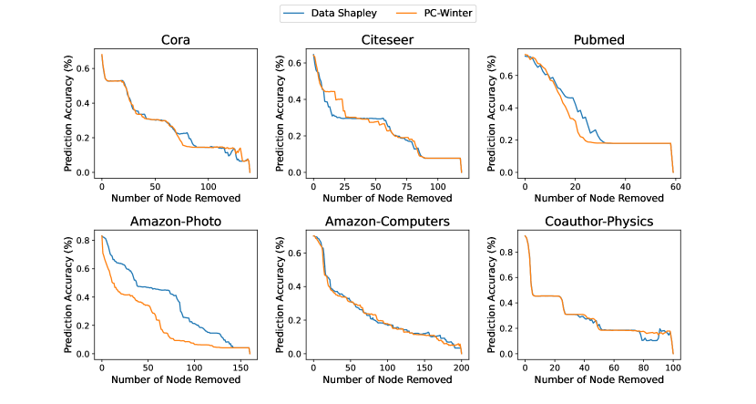
Here, we perform node dropping experiment employing the aggregated value define in the main-body of paper, to demonstrate that PC-Winter can capture the heterogeneous influence of labeled nodes. As shown in the Figure 9, both PC-Winter and Data Shapley demonstrate effectiveness in capturing the diverse contributions of labeled nodes to the model’s performance. Particularly in the Pubmed and Amazon-Photo datasets, PC-Winter exhibits better performance compared to Data Shapley. In other datasets, such as Cora, Citeseer, and Coauthor-Physics, PC-Winter shows results that are on par with Data Shapley.
Appendix G Experimental Details
G.1 Datasets
We assess the proposed approach on six real-world benchmark datasets. These include three citation graphs, Cora, Citeseer and Pubmed (Sen et al., 2008) and two Amazon Datasets, Amazon-Photo and Amazon-Computer, and Coauther-Physics (Shchur et al., 2018). The detailed statistics of datasets are summarized in Table 2.
Dataset # Node # Edge # Class # Feature # Train/Val/Test Cora 2,708 5,429 7 1,433 140 / 500 / 1,000 Citeseer 3,327 4,732 6 3,703 120 / 500 / 1,000 Pubmed 19,717 44,338 3 500 60 / 500 / 1,000 Amazon-Photo 7,650 119,081 8 745 160 / 20% / 20% Amazon-Computer 13,752 245,861 10 767 200 / 20% / 20% Coauthor-Physics 34,493 247,962 8 745 100 / 20% / 20%
G.2 Split Settings
In the conducted experiments, we split each graph into disjoint subgraphs: training graph , validation graph , and test graph . The training graph is constructed without any nodes from the validation or test set. Correspondingly, edges connecting to a validation node or a testing node are also removed from the training graph. For the validation graph and the testing graph , only edges with both nodes within the respective node sets are retained, which is aligned with the inductive setting in prior work (Zhang et al., 2021). We utilize to train the GNN model, which is evaluated on for obtaining the data values for elements. The test graph is utilized to evaluate the effectiveness of the obtained values. In the case of the specific split for each dataset, for the citation networks, we adopt public train/val/test splits in our experiments. For the remaining datasets, we randomly select 20 labeled nodes per class for training, 20% nodes for validation and 20% nodes as the testing set.
G.3 Convergence Criteria
Convergence Criterion. For permutation-based data valuation methods such as Data Shapley and PC-Winter, we follow convergence criteria similar to the one applied in prior work (Ghorbani & Zou, 2019) to determine the number of permutations for approximating data values:
where is the estimated value for the data element using the first sampled permutations.
Time Limit. For larger datasets, sampling a sufficient number of permutations for converged data values could be impractical in time. To address this and to stay within a realistic scope, we cap the computation time at 120 GPU hours on NVIDIA Titan RTX, after which the calculation is terminated.
G.4 Truncation Ratios and Hyper-parameters
Table 3 includes the hyper-parameters and truncation ratios used for value estimation.
Dataset Truncation Ratio Learning Rate Epoch Weight Decay Cora 0.5-0.7 0.01 200 5e-4 Citeseer 0.5-0.7 0.01 200 5e-4 Pubmed 0.5-0.7 0.01 200 5e-4 Amazon-Photo 0.7-0.9 0.1 200 0 Amazon-Computer 0.7-0.9 0.1 200 0 Coauthor-Physics 0.7-0.9 0.01 30 5e-4
G.5 Baselines
G.5.1 Dropping High-Value Nodes
Here, we introduce the baselines used for comparison to validate the effectiveness of the proposed method in the dropping node experiment:
-
•
Random Value: It assigns nodes with random values, which leads to random ranking without any specific pattern or correlation to the node’s features.
-
•
Degree-based Value: A node is assigned its degree as its value, assuming that a node’s importance in the graph is indicated by its degree.
-
•
Leave-one-out (LOO): This method calculates a node’s value based on its marginal contribution compared to the rest of the training nodes. Specifically, the value assigned to each node is its marginal utility, calculated as , where denotes the training graph excluding node . The utility function measures the model’s validation performance when trained on the given graph. In essence, the drop in performance due to the removal of a node is treated as the value of that node.
-
•
Data Shapley: The node values are approximated with the Monte Carlo sampling method of Data Shapley (Ghorbani & Zou, 2019) by treating both labeled nodes and unlabeled nodes as players. Notably, we only include those unlabeled nodes within the -hop neighbors of labeled nodes in the evaluation process. There are two approximation methods: Truncated Monte Carlo approximation and Gradient Shapley in (Ghorbani & Zou, 2019). We adopt the Truncated Monte Carlo approximation as it consistently outperforms the other variants in various experiments.
G.5.2 Adding High-Value Edges
Here are the detailed descriptions on the baselines applied in the edge adding experiment.
-
•
Random Value: it assigns edges with random values, reflecting a baseline where no information are used for differentiating the importance of edges.
-
•
Edge-Betweeness: the Edge-Betweeness of an edge is the the fraction of all pairwise shortest paths that go through . This classic approach assesses an edge’s importance based on its role in the overall network connectivity.
-
•
Leave-one-out (LOO): This method calculates a edge ’s value based on its marginal contribution compared to the rest of the training graph. In specific, Here, represents an edge in the training graph , and refers to the training graph excluding the edge .
Appendix H Ablation Study and Parameter Analysis
H.1 Ablation Study
This Appendix Section offers an in-depth ablation analysis across full six datasets to investigates the necessity of both Level Constraint and Precedence Constraint in defining an effective graph value. The results, as shown in Figure 10, consistently demonstrate across all datasets that the absence of either constraint leads to a degraded result when compared to the one incorporating both. This underscores the importance of both two constraints in capturing the contributions of graph elements to overall model performance.
H.2 The Impact of Permutation Number
This part expands upon the permutation analysis presented in the main paper. It provides comprehensive results across various datasets, illustrating how different numbers of sample permutations impact the accuracy of PC-Winter. The results of full datasets are shown in Figure 11.
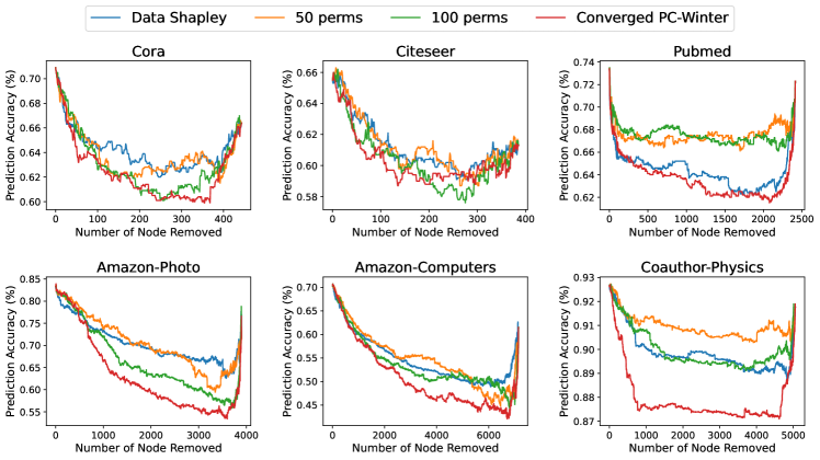
The results reveals that increasing the number of permutations generally improves the performance and accuracy of the valuation. PC-Winter also show robust results even with a limited number of permutations, highlighting its effectiveness. The phenomenon is consistent across all datasets where our approach with just 50 to 100 permutations manages to compete closely with the fully converged Data Shapley, emphasizing the efficiency of PC-Winter in various settings.
H.3 The Impact of Truncation Ratios
Our approach involves truncating the iterations involving the first and second-hop neighbors of a labeled node during value estimation. Here, we investigate the impact of truncation proportion on overall performance, using the same number of permutations as in our primary node-dropping experiment. As shown in Figure 7, we adjusted the truncation ratios for the Citation Network datasets. The ratios ranged from truncating 50% of the first-hop and 70% of the second-hop neighbors (0.5-0.7), up to 90% truncation for either first-hop (0.9-0.7) or second-hop (0.5-0.9) neighbors. For the Cora and Citeseer datasets, increasing truncation at the first-hop level had a minimal impact on performance, and PC-Winter still significantly outperformed Data Shapley. In the case of the Pubmed dataset, more extensive truncation at the first-hop level notably reduced performance. Regarding large datasets such as the Amazon, while truncation at either the first or second-hop levels had a marginal negative effect on performance, PC-Winter ’s estimated data values generally remained superior to results of Data Shapley.
In addition, we provide a detailed analysis of our truncation strategy across other datasets. It includes results not presented in the main text, focusing on the impact of limiting model retraining times to the first and second-hop neighbors in value estimation. We investigate the impact of truncation proportion on overall performance, using the same number of permutations as in our primary node-dropping experiment. The findings on full datasets are illustrated in Figure 12. Specifically, our findings reveal that in datasets like Cora and Citeseer, adjusting truncation primarily at the first-hop level has a negligible impact on the accuracy of node valuation, with PC-Winter still maintaining a considerable advantage over Data Shapley. For large datasets such as the Amazon-Photo, Amazon-Computers and Coauther-Physics, while truncations had a marginal negative effect on performance, PC-Winter ’s estimated data values generally remained better than Data Shapley. This analysis indicates that PC-Winter can afford to employ larger truncation, enhancing computational efficiency without substantially sacrificing the quality of data valuation.
Dataset Truncation PC-Winter Perm Time (hrs) Data Shapley Perm Time (hrs) Cora 0.5-0.7 0.013 0.024 Citeseer 0.5-0.7 0.018 0.037 Pubmed 0.5-0.7 0.025 0.285 Amazon-Photo 0.7-0.9 0.211 1.105 Amazon-Computer 0.7-0.9 0.662 3.566 Coauthor-Physics 0.7-0.9 0.119 2.642
PC-Winter Data Shapley Dataset Perm Number Total GPU hour Perm Number Total GPU hour Cora 325.00 4.25 327.00 8.00 Citeseer 291.00 5.24 279.00 10.32 Pubmed 316.00 7.82 281.00 80.13 Amazon-Photo 418.00 88.12 109.00 120.39 Amazon-Computer 181.00 119.83 33.00 117.68 Coauthor-Physics 460.00 54.75 45.00 118.87
H.4 Efficiency Analysis
Here, we compare the computational time required for each permutation using both our proposed method and the Data Shapley approach. As detailed in Table 4, the results indicate that PC-Winter requires significantly less time to compute permutations across various datasets. Specifically, for the Cora dataset, PC-Winter completes permutations in approximately half the time required by Data Shapley. Moving to larger datasets, the efficiency of PC-Winter becomes even more pronounced. For instance, in the Amazon-Computer dataset, PC-Winter’s permutation time is only a fraction of what is required by Data Shapley —PC-Winter takes slightly over half an hour whereas Data Shapley exceeds three and a half hours. This consistent reduction in permutation time demonstrates the computational advantage of PC-Winter, particularly when handling large graphs.
For more information, we also compare the total computational time required for value estimation using both PC-Winter and the Data Shapley approach. As detailed in Table 5, for the Cora dataset, PC-Winter and Data Shapley perform a similar number of permutations, 325 and 327 respectively, but PC-Winter completes these with considerably fewer GPU hours, cutting the time nearly in half. In the case of Citeseer, PC-Winter performs slightly more permutations than Data Shapley (291 vs 279), yet it still requires significantly less total GPU time, indicating enhanced efficiency. The contrast is ever larger when it comes to the Pubmed dataset: PC-Winter reduces the total GPU hours to less than a tenth of the time required by Data Shapley. This substantial reduction in computational time highlights the efficiency of PC-Winter. In the case of larger datasets like Amazon-Photo, Amazon-Computer, and Physics, PC-Winter successfully converged in two out of the three cases. In contrast, Data Shapley did not converge in these larger datasets. This demonstrates the efficiency and effectiveness of PC-Winter, even in more computational challenging scenarios.
Combining the insights from the Permutation Analysis shown in Figure 11 with the Permutation Time Table 4, we observe that for datasets such as Cora, Citeseer, Amazon-Photo, and Amazon-Computer around 50 permutations are sufficient for PC-Winter to achieve performance comparable to that of Data Shapley. Simple calculations demonstrate that our method is significantly faster than Data Shapley in achieving similar performance levels. For instance, in the Cora dataset, the speedup factor is , and for the Citeseer dataset, it is . The speedup factors for Amazon-Photo and Amazon-Computer are , and , respectively. For Coauthor-Physics, it takes about PC-Winter permutations to match the performance of Data Shapley, which implies a speedup factor of . In conclusion, PC-Winter can achieve stronger performance than Data Shapley using the same or even less time. Furthermore, it takes PC-Winter much less time to achieve comparable performance as Data Shapley.
Notably, though PC-Winter is significantly more efficient than Data Shapley, its scalability is still limited, and future work in further improving its efficiency is desired.