Sample, estimate, aggregate:
A recipe for causal discovery foundation models

Abstract

Causal discovery, the task of inferring causal structure from data, promises to accelerate scientific research, inform policy making, and more. However, the per-dataset nature of existing causal discovery algorithms renders them slow, data hungry, and brittle. Inspired by foundation models, we propose a causal discovery framework where a deep learning model is pretrained to resolve predictions from classical discovery algorithms run over smaller subsets of variables. This method is enabled by the observations that the outputs from classical algorithms are fast to compute for small problems, informative of (marginal) data structure, and their structure outputs as objects remain comparable across datasets. Our method achieves state-of-the-art performance on synthetic and realistic datasets, generalizes to data generating mechanisms not seen during training, and offers inference speeds that are orders of magnitude faster than existing models.

1 Introduction

A fundamental aspect of scientific research is to discover and validate causal hypotheses involving variables of interest. Given observations of these variables, the goal of causal discovery algorithms is to extract such hypotheses in the form of directed graphs, in which edges denote causal relationships (Spirtes et al., 2001). In much of basic science, however, classical statistics remain the de facto basis of data analysis (Replogle et al., 2022). Key barriers to widespread adoption of causal discovery algorithms include their high data requirements and their computational intractability on larger problems.

Current causal discovery algorithms follow two primary approaches that differ in their treatment of the underlying causal graph. Discrete optimization algorithms explore the super-exponential space of graphs by proposing and evaluating changes to a working graph (Glymour et al., 2019). While these methods are quite fast on small graphs, the combinatorial space renders them intractable for exploring larger structures, with hundreds or thousands of nodes. Furthermore, their correctness is tied to hypothesis tests, whose results can be erroneous for noisy datasets, especially as graph sizes increase. More recently, a number of works have reframed the discrete graph search as a continuous optimization over weighted adjacency matrices (Zheng et al., 2018; Brouillard et al., 2020). These continuous optimization algorithms often require that a generative model be fit to the full data distribution, a difficult task when the number of variables increases but the data remain sparse.

In this work, we present Sea: Sample, Estimate, Aggregate, a blueprint for developing causal discovery foundation models that enable fast inference on new datasets, perform well in low data regimes, and generalize to causal mechanisms beyond those seen during training. Our approach is motivated by two observations. First, while classical causal discovery algorithms scale poorly, their bottleneck lies in the exponential search space, rather than individual independence tests. Second, in many cases, statistics like global correlation or inverse covariance are indeed strong indicators for a graph’s overall connectivity. Therefore, we propose to leverage 1) the estimates of classical algorithms over small subgraphs, and 2) global graph-level statistics, as inputs to a deep learning model, pretrained to resolve these statistical descriptors into causal graphs.

Theoretically, we prove that given only marginal estimates over subgraphs, it is possible to recover causally sound global graphs; and that our proposed model has the capacity to recapitulate such reasoning. Empirically, we implement instantiations of Sea using an axial-attention based model (Ho et al., 2020) which takes as input, inverse covariance and estimates from the classical FCI or GIES algorithms (Spirtes et al., 1995; Hauser & Bühlmann, 2012). We conduct thorough comparison to three classical baselines and five deep learning approaches. Sea attains the state-of-the-art results on synthetic and real-world causal discovery tasks, while providing 10-1000x faster inference. While these experimental results reflect specific algorithms and architectures, the overall framework accepts any combination of sampling heuristics, classical causal discovery algorithms, and statistical features. To summarize, our contributions are as follows.

1. To the best of our knowledge, we are the first to propose a method for building fast, robust, and generalizable foundation models for causal discovery.

2. We show that both our overall framework and specific architecture have the capacity to reproduce causally sound graphs from their inputs.

3. We attain state-of-the-art results on synthetic and realistic settings, and we provide extensive experimental analysis of our model.

2 Background and related work

2.1 Causal graphical models

A causal graphical model is a directed, acyclic graph $G=(V,E)$, where each node $i\in V$ corresponds to a random variable $X_{i}\in X$ and each edge $(i,j)\in E$ represents a causal relationship from $X_{i}\to X_{j}$.

We assume that the data distribution $P_{X}$ is Markov to $G$,

$$\forall i\in V,X_{i}\perp\!\!\!\perp V\setminus\left(X_{\delta_{i}}\cup X_{\pi_{i}}\right)\mid X_{\pi_{j}}$$ (1)

where $\delta_{i}$ is the set of descendants of node $i$ in $G$, and $\pi_{i}$ is the set of parents of $i$. In addition, we assume that $P_{X}$ is minimal and faithful – that is, $P_{X}$ does not include any independence relationships beyond those implied by applying the Markov condition to $G$ (Spirtes et al., 2001).

Causal graphical models allow us to perform interventions on nodes $i$ by setting conditional $P(X_{i}\mid X_{\pi_{i}})$ to a different distribution $\tilde{P}(X_{i}\mid X_{\pi_{i}})$.

2.2 Causal discovery

Given a dataset $D\sim P_{X}$, the goal of causal discovery is to recover $G$. There are two main challenges. First, the number of possible graphs is super-exponential in the number of nodes $N$, so causal discovery algorithms must navigate this combinatorial search space efficiently. In terms of graph size, the limits of current algorithms range from tens of nodes (Hägele et al., 2023) to hundreds of nodes (Lopez et al., 2022), where simplifying assumptions regarding the graph structure are often made in the latter case. Second, depending on data availability and the underlying data generation process, causal discovery algorithms may or may not be able to recover $G$ in practice. In fact, many algorithms are only analyzed in the infinite-data regime and require at least thousands of data samples for reasonable empirical performance (Spirtes et al., 2001; Brouillard et al., 2020).

Causal discovery is also used in the context of pairwise relationships (Zhang & Hyvarinen, 2012; Monti et al., 2019), as well as for non-stationary (Huang et al., 2020) and time-series (Löwe et al., 2022) data. However, this work focuses on causal discovery for stationary graphs, so we will discuss the two main approaches to causal discovery in this setting.

Discrete optimization methods make atomic changes to a proposal graph until a stopping criterion is met. Constraint-based algorithms identify edges based on conditional independence tests, and their correctness is inseparable from the empirical results of those tests (Glymour et al., 2019), whose statistical power depends directly on dataset size. These include the FCI and PC algorithms in the observational case (Spirtes et al., 1995), and the JCI algorithm in the interventional case (Mooij et al., 2020).

Score-based methods also make iterative modifications to a working graph, but their goal is to maximize a continuous score over the discrete space of all valid graphs, with the true graph at the optimum. Due to the intractable search space, these methods often make decisions based on greedy heuristics. Classic examples include GES (Chickering, 2002), GIES (Hauser & Bühlmann, 2012), CAM (Bühlmann et al., 2014), and LiNGAM (Shimizu et al., 2006).

Continuous optimization approaches recast the combinatorial space of graphs into a continuous space of weighted adjacency matrices. Many of these works train a generative model to learn the empirical data distribution, which is parameterized through the adjacency matrix (Zheng et al., 2018; Lachapelle et al., 2020; Brouillard et al., 2020). Others focus on properties related to the empirical data distribution, such as a relationship between the underlying graph and the Jacobian of the learned model (Reizinger et al., 2023), or between the Hessian of the data log-likelihood and the topological ordering of the nodes (Sanchez et al., 2023). While these methods bypass the combinatorial search over discrete graphs, they still require copious data and time to train accurate generative models of the data distributions.

2.3 Foundation models

The concept of foundation models has revolutionized the machine learning workflow in a variety of disciplines: instead of training domain-specific models from scratch, we can query a pretrained, general-purpose “foundation” model (Radford et al., 2021; Brown et al., 2020; Bommasani et al., 2022). Recent work has explored foundation models for causal inference (Zhang et al., 2023), but this method addresses causal inference rather than causal discovery, so it assumes that the causal structures are already known.

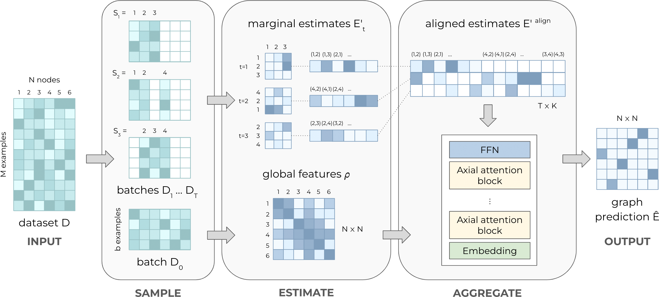
Figure 1: An overview of the Sea inference procedure. Given a new dataset, we 1) sample batches and subsets of nodes, 2) estimate marginal graphs and global statistics over these batches, and 3) aggregate these features using a pretrained model to obtain the underlying causal graph. Raw data are depicted in green, and graph-related features are depicted in blue.

3 Methods

We present Sea, a framework for developing fast and scalable causal discovery foundation models. We follow two key insights. First, while classical causal discovery algorithms scale poorly to large graphs, they are highly performant on small graphs. Second, in many cases, simple statistics like global correlation or inverse covariance are strong baselines for a graph’s overall connectivity. Our framework combines global statistics and marginal estimates (the outputs of classical causal discovery algorithms on subsets of nodes) as inputs to a deep learning model, pretrained to aggregate these features into causal graphs (Section 3.1). As proofs of concept, we describe instantiations of Sea using specific algorithms and architectures (Sections 3.2, 3.3). Finally, we prove that our algorithm has the capacity to produce sound causal graphs, in theory and in context of our implementation (Section 3.4).

3.1 Causal discovery framework

Sea is a causal discovery framework that learns to resolve statistical features and estimates of marginal graphs into a global causal graph. The inference procedure is depicted in Figure 1. Specifically, given a new dataset $D\in\mathbb{R}^{M\times N}$ faithful to graph $G=(V,E)$, we apply the following stages.

Sample: takes as input dataset $D$; and outputs data batches $\{D_{0},D_{1},\dots,D_{T}\}$ and node subsets $\{S_{1},\dots,S_{T}\}$.

1. Sample $T+1$ batches of $b\ll M$ observations uniformly at random from $D$.

2. Compute selection scores $\alpha\in(0,1)^{N\times N}$ over $D_{0}$ (e.g. inverse covariance).

3. Sample $T$ node subsets of size $k$. Each subset $S_{t}\subseteq V$ is constructed iteratively, with additional nodes sampled one at a time with probability proportional to $\sum_{j\in S_{t}}\alpha_{i,j}$ (details in Section B.6).

Estimate: takes as inputs data batches and node subsets; and outputs global statistics $\rho$ and marginal estimates $\{E^{\prime}_{1},\dots,E^{\prime}_{T}\}$.

1. Compute global statistics $\rho\in\mathbb{R}^{N\times N}$ over $D_{0}$.

2. Run causal discovery algorithm $f$ to obtain marginal estimates $f(D_{t}[S_{t}])=E^{\prime}_{t}$ for $t=1\dots T$.

We use $D_{t}[S_{t}]$ to denote the observations in $D_{t}$ that correspond only to the variables in $S_{t}$. Each estimate $E^{\prime}_{t}$ is a $k\times k$ adjacency matrix, corresponding to the $k$ nodes in $S_{t}$.

Aggregate: takes as inputs global statistics, marginal estimates, and node subsets. A pretrained aggregator model outputs the predicted global causal graph $\hat{E}\in(0,1)^{N\times N}$.

The aggregator’s architecture is agnostic to the assumptions of the underlying causal discovery algorithm $f$ (e.g. (non)linearity, observational vs. interventional). Therefore, we can freely swap out $f$ and the training datasets to train aggregators with different implicit assumptions, without modifying the architecture itself. Here, our aggregator is pretrained over a diverse set of graph sizes, structures, and data generating mechanisms (details in Section 4.1).

Figure 2: Aggregator architecture. Marginal graph estimates and global statistics are first embedded into the model dimension, and 1D positional embeddings are added along both rows and columns. These combined embeddings pass through a series of axial attention blocks, which attend to the graph estimates and the global features. The final layer global features pass through a feedforward network to predict the causal graph.

3.2 Model architecture

The core module of Sea is the aggregator (Figure 2), implemented as a sequence of axial attention blocks. The aggregator takes as input global statistics $\rho\in\mathbb{R}^{N\times N}$, marginal estimates $E^{\prime}_{1\dots T}\in\mathcal{E}^{T\times k\times k}$, and node subsets $S_{1\dots T}\in[N]^{T\times k}$, where $\mathcal{E}$ is the set of output edge types for the causal discovery algorithm $f$.

We project global statistics into the model dimension via a learned linear projection matrix $W_{\rho}:\mathbb{R}\to\mathbb{R}^{d}$, and we embed edge types via a learned embedding $\text{ebd}_{\mathcal{E}}:\mathcal{E}\to\mathbb{R}^{d}$. To collect estimates of the same edge over all subsets, we align entries of $E^{\prime}_{1\dots T}$ into $E^{{}^{\prime}\textrm{align}}_{T}\in\mathcal{E}^{T\times K}$

$$E^{{}^{\prime}\textrm{align}}_{t,e=(i,j)}=\begin{cases}E^{\prime}_{t,i,j}&\textrm{ if }i\in S_{t},j\in S_{t}\\ 0&\textrm{ otherwise}\end{cases}$$ (2)

where $t$ indexes into the subsets, $e$ indexes into the set of unique edges, and $K$ is the number of unique edges.

We add learned 1D positional embeddings along both dimensions of each input,

$$\textrm{pos-ebd}(\rho_{i,j})=~{} \textrm{ebd}_{\text{node}}(i^{\prime})+\textrm{ebd}_{\text{node}}(j^{\prime})$$

$$\textrm{pos-ebd}(E^{{}^{\prime}\textrm{align}}_{t,e})=~{} \textrm{ebd}_{\text{time}}(t)$$

$$+\textrm{FFN}([\textrm{ebd}_{\text{node}}(i^{\prime}),\textrm{ebd}_{\text{node}}(j^{\prime})])$$

where $i^{\prime},j^{\prime}$ index into a random permutation on $V$ for invariance to node permutation and graph size. Due to the (a)symmetries of their inputs, $\textrm{pos-ebd}(\rho_{i,j})$ is symmetric, while $\textrm{pos-ebd}(E^{{}^{\prime}\textrm{align}}_{t,e})$ considers the node ordering. In summary, the inputs to our axial attention blocks are

$$h^{\rho}_{i,j} =(W_{\rho}\rho)_{i,j}+\textrm{pos-ebd}(\rho_{i,j})$$ (3)

$$h^{E}_{t,e} =\textrm{ebd}_{\mathcal{E}}(E^{{}^{\prime}\textrm{align}}_{t,e})+\textrm{pos-ebd}(E^{{}^{\prime}\textrm{align}}_{t,e})$$ (4)

for $i,j\in[N]^{2}$, $t\in[T]$, $e\in[K]$.

Axial attention

An axial attention block contains two axial attention layers (marginal estimates, global features) and a feed-forward network (Figure 2, right).

Given a 2D input, an axial attention layer attends first along the rows, then along the columns. For example, given a matrix of size (R,C,d), one pass of the axial attention layer is equivalent to running standard self-attention along C with batch size R, followed by the reverse. For marginal estimates, R is the number of subsets $T$, and C is the number of unique edges $K$. For global features, R and C are both the total number of vertices $N$.

Following (Rao et al., 2021), each self-attention mechanism is preceded by layer normalization and followed by dropout, with residual connections to the input,

$$x=x+\text{Dropout}(\text{Attn}(\text{LayerNorm}(x))).$$ (5)

We pass messages between the marginal and global layers to propagate information. Let $\phi_{E,\ell}$ be marginal layer $\ell$, let $\phi_{\rho,\ell}$ be global layer $\ell$, and let $h^{\cdot,\ell}$ denote the hidden representations out of layer $\ell$.

The marginal to global message $m^{E\to\rho}\in\mathbb{R}^{N\times N\times d}$ contains representations of each edge averaged over subsets,

$$m^{E\to\rho,\ell}_{i,j} =\begin{cases}\frac{1}{T_{e}}\sum_{t}h^{E,\ell}_{t,e=(i,j)}&\textrm{ if }\exists S_{t},i,j\in S_{t}\\ \epsilon&\textrm{ otherwise.}\end{cases}$$ (6)

where $T_{e}$ is the number of $S_{t}$ containing $e$, and missing entries are padded to learned constant $\epsilon$. The global to marginal message $m^{\rho\to E}\in\mathbb{R}^{K\times d}$ is simply the hidden representation itself,

$$m^{\rho\to E,\ell}_{t,e=(i,j)} =h^{\rho,\ell}_{i,j}.$$ (7)

We incorporate these messages as follows.

$$h^{E,\ell} =\phi_{E,\ell}(h^{E,\ell-1})$$ (marginal feature) (8)

$$h^{\rho,\ell-1} \leftarrow W^{\ell}\left[h^{\rho,\ell-1},m^{E\to\rho,\ell}\right]$$ (marginal to global) (9)

$$h^{\rho,\ell} =\phi_{\rho,\ell}(h^{\rho,\ell-1})$$ (global feature) (10)

$$h^{E,\ell} \leftarrow h^{E,\ell}+m^{\rho\to E,\ell}$$ (global to marginal) (11)

$W^{\ell}\in\mathbb{R}^{2d\times d}$ is a learned linear projection, and $[\cdot]$ denotes concatenation.

Graph prediction

For each pair of vertices $i\neq j\in V$, we predict $e=0,1$, or $2$ for no edge, $i\to j$, and $j\to i$ respectively. This constraint may be omitted for cyclic graphs. We do not additionally enforce that our predicted graphs are acyclic, similar in spirit to (Lippe et al., 2022).

Given the output of the final axial attention block, $h^{\rho}$, we compute logits

$$z_{\{i,j\}}=\text{FFN}\left(\left[h^{\rho}_{i,j},h^{\rho}_{j,i}\right]\right)\in\mathbb{R}^{3}$$ (12)

which correspond to probabilities after softmax normalization. The overall output $\hat{E}\in\{0,1\}^{N\times N}$ is supervised by the ground truth $E$, and our model is trained with cross entropy loss and L2 weight regularization.

3.3 Implementation details

We computed inverse covariance as the global statistic and selection score, due to its relationship to partial correlation and ease of computation. For comparison to additional statistics, see C.2. We chose the constraint-based FCI algorithm in the observational setting (Spirtes et al., 2001), and the score-based GIES algorithm in the interventional setting (Hauser & Bühlmann, 2012). For discussion regarding alternative algorithms, see B.5. We sample batches of size $b=500$ over $k=5$ nodes each (analysis in C.1).

Our model was implemented with 4 layers with 8 attention heads and hidden dimension 512. Our model was trained using the AdamW optimizer with a learning rate of 1e-4 (Loshchilov & Hutter, 2019). Please see B.3 for additional details regarding hyperparameters.

3.4 Theoretical analyses

Our theoretical contributions span two aspects.

1. We formalize the notion of marginal estimates and prove that given sufficient marginal estimates, it is possible to recover a pattern faithful to the global causal graph (Theorem 3.4). We provide bounds on the number of marginal estimates required and motivate global statistics as an efficient means to reduce this bound (Propositions 3.4, 3.4).

2. We show that our proposed axial attention has the capacity to recapitulate the reasoning required for this task. In particular, we show that a stack of 3 axial attention blocks can recover the skeleton and v-structures in $O(N)$ width (Theorem 3.4).

We state our key results below, and direct the reader towards Appendix A for all proofs. Our proofs assume only that the edge estimates are correct. We do not impose any functional requirements, and any appropriate independence test may be used. We discuss robustness and stability in A.4.

[Marginal estimate resolution]theoremthmresolve Let $G=(V,E)$ be a directed acyclic graph with maximum degree $d$. For $S\subseteq V$, let $E^{\prime}_{S}$ denote the marginal estimate over $S$. Let $\mathcal{S}_{d}$ denote the superset that contains all subsets $S\subseteq V$ of size at most $d$. There exists a mapping from $\{E^{\prime}_{S}\}_{S\in\mathcal{S}_{d+2}}$ to pattern $E^{*}$, faithful to $G$.

Theorem 3.4 formalizes the intuition that it requires at most $d$ independence tests to check whether two nodes are independent, and to estimate the full graph structure, it suffices to run a causal discovery algorithm on subsets of $d+2$.

[Skeleton bounds]propositionpropBoundSkeleton Let $G=(V,E)$ be a directed acyclic graph with maximum degree $d$. It is possible to recover the undirected skeleton $C=\{\{i,j\}:(i,j)\in E\}$ in $O(N^{2})$ estimates over subsets of size $d+2$.

If we only leverage marginal estimates, we must check at least $\binom{N}{2}$ subsets to cover each edge at least once. However, we can often approximate the skeleton via global statistics such as correlation, allowing us to use marginal estimates more efficiently, towards answering orientation questions.

[V-structures bounds]propositionpropBoundV Let $G=(V,E)$ be a directed acyclic graph with maximum degree $d$ and $\nu$ v-structures. It is possible to identify all v-structures in $O(\nu)$ estimates over subsets of at most size $d+2$.

[Model capacity]theoremthmpower Given a graph $G$ with $N$ nodes, a stack of $L$ axial attention blocks has the capacity to recover its skeleton and v-structures in $O(N)$ width, and propagate orientations on paths of $O(L)$ length.

Existing literature on the universality and computational power of vanilla Transformers (Yun et al., 2019; Pérez et al., 2019) rely on generous assumptions regarding depth or precision. Here, we show that our axial attention-based model can implement the specific reasoning required to resolve marginal estimates under realistic conditions.

4 Experimental setup

We pretrained Sea models on synthetic training datasets only and ran inference on held-out testing datasets, which include both seen and unseen causal mechanisms. All baselines were trained and/or run from scratch on each testing dataset using their published code and hyperparameters.

4.1 Data settings

We evaluate our model across diverse synthetic datasets, simulated mRNA datasets (Dibaeinia & Sinha, 2020), and a real protein expression dataset (Sachs et al., 2005).

The synthetic datasets were constructed based on Table 1. For each synthetic dataset, we first sample a graph based on the desired topology and connectivity. Then we topologically sort the graph and sample observations starting from the root nodes, using random instantiations of the designated causal mechanism (details in B.1). We generated 90 training, 5 validation, and 5 testing datasets for each combination (8160 total). To evaluate our model’s capacity to generalize to new functional classes, we reserve the Sigmoid and Polynomial causal mechanisms for testing only. We include details on our synthetic mRNA datasets in Appendix C.3.

4.2 Causal discovery metrics

Our causal discovery experiments consider both discrete and continuous metrics. In addition to standard metrics like SHD (Tsamardinos et al., 2006), we advocate for the inclusion of continuous metrics, as neural networks can be notoriously uncalibrated (Guo et al., 2017), and arbitrary discretization thresholds reflect an incomplete picture of model performance (Schaeffer et al., 2023). For example, the graph of all 0s has the same accuracy as a graph’s undirected skeleton, though the two differ vastly in information content (Table 2). For all continuous metrics, we exclude the diagonal from evaluation, since several baselines manually set it to zero (Brouillard et al., 2020; Lopez et al., 2022).

SHD: Structural Hamming distance is the minimum number of edge edits required to match two graphs (Tsamardinos et al., 2006). Discretization thresholds are as published.

Table 1: Synthetic data generation settings. The symbol $*$ denotes training only, and $\dagger$ denotes testing only. We take the Cartesian product of all parameters for our settings. (Non)-additive refers to (non)-additive Gaussian noise. Details regarding the causal mechanisms can be found in B.1

Parameter	Values
Nodes $(N)$	$10,20,100$
Edges	$N,2N^{*},3N^{*},4N$
Points	$1000N$
Interventions	$N$
Topology	Erdős-Rényi, Scale Free
Mechanism	Linear, NN additive, NN non-additive, Sigmoid additive†, Polynomial additive†

Table 2: Motivating continuous metrics in causal discovery. SHD alone is a poor measure of prediction quality, as it fails to distinguish between the graph of all 0s and the undirected skeleton. Metrics reported on Sachs.

	SHD $\downarrow$	mAP $\uparrow$	AUC $\uparrow$	EdgeAcc $\uparrow$
Ground truth	0	1	1	1
Undirected	17	0.5	0.92	0
All 0s	17	0.14	0.5	0

mAP: Mean average precision computes the area under precision-recall curve per edge and averages over the graph. The random guessing baseline depends on the positive rate.

AUC: Area under the ROC curve (Bradley, 1997) computed per edge (binary prediction) and averaged over the graph. For each edge, 0.5 indicates random guessing, while 1 indicates perfect performance.

Edge orientation accuracy: We compute the accuracy of edge orientations as

$$\text{EdgeAcc}=\frac{\sum_{(i,j)\in E}\mathbbm{1}\{P(i,j)>P(j,i)\}}{\|E\|}.$$ (13)

Since this quantity is normalized by the size of $E$, it is invariant to the positive rate. In contrast to edge orientation F1 (Geffner et al., 2022), this quantity is also invariant to the assignment of forward/reverse edges as positive/negative. By design, symmetric predictions (like the undirected graph) have an edge orientation accuracy of 0.

Table 3: Causal discovery results on synthetic datasets. Each setting encompasses 5 distinct Erdős-Rényi graphs. The symbol $\dagger$ indicates that Sea was not pretrained on this setting. Runtimes are plotted in Figure 3. Details regarding baselines can be found in B.2.

$N$	$E$	Model	Linear		NN add.		NN non-add.		Sigmoid†		Polynomial†
			mAP $\uparrow$	SHD $\downarrow$	mAP $\uparrow$	SHD $\downarrow$	mAP $\uparrow$	SHD $\downarrow$	mAP $\uparrow$	SHD $\downarrow$	mAP $\uparrow$	SHD $\downarrow$
10	10	Dcdi-G	$0.74\scriptstyle\pm 0.2$	$2.8\scriptstyle\pm 2.0$	$0.79\scriptstyle\pm 0.1$	$\textbf{2.2}\scriptstyle\pm 2.5$	$0.89\scriptstyle\pm 0.1$	$\textbf{1.0}\scriptstyle\pm 0.6$	$0.46\scriptstyle\pm 0.2$	$5.8\scriptstyle\pm 2.7$	$0.41\scriptstyle\pm 0.1$	$8.9\scriptstyle\pm 5.3$
		Dcdi-Dsf	$0.82\scriptstyle\pm 0.2$	$2.0\scriptstyle\pm 2.6$	$0.57\scriptstyle\pm 0.2$	$3.0\scriptstyle\pm 2.3$	$0.50\scriptstyle\pm 0.2$	$4.2\scriptstyle\pm 1.3$	$0.38\scriptstyle\pm 0.2$	$6.3\scriptstyle\pm 2.7$	$0.29\scriptstyle\pm 0.1$	$11.2\scriptstyle\pm 5.2$
		Dcd-Fg	$0.45\scriptstyle\pm 0.2$	$20.4\scriptstyle\pm 2.9$	$0.41\scriptstyle\pm 0.1$	$21.2\scriptstyle\pm 3.3$	$0.59\scriptstyle\pm 0.1$	$19.2\scriptstyle\pm 3.8$	$0.40\scriptstyle\pm 0.2$	$19.8\scriptstyle\pm 3.6$	$0.50\scriptstyle\pm 0.2$	$18.5\scriptstyle\pm 5.1$
		DiffAn	$0.25\scriptstyle\pm 0.1$	$14.0\scriptstyle\pm 4.4$	$0.32\scriptstyle\pm 0.2$	$13.6\scriptstyle\pm 12.9$	$0.12\scriptstyle\pm 0.0$	$21.8\scriptstyle\pm 6.7$	$0.24\scriptstyle\pm 0.1$	$12.0\scriptstyle\pm 5.0$	$0.20\scriptstyle\pm 0.1$	$15.0\scriptstyle\pm 6.1$
		Deci	$0.18\scriptstyle\pm 0.1$	$19.4\scriptstyle\pm 4.4$	$0.16\scriptstyle\pm 0.1$	$13.8\scriptstyle\pm 5.8$	$0.23\scriptstyle\pm 0.1$	$16.2\scriptstyle\pm 2.6$	$0.29\scriptstyle\pm 0.2$	$13.9\scriptstyle\pm 6.9$	$0.46\scriptstyle\pm 0.2$	$7.8\scriptstyle\pm 3.9$
		InvCov	$0.49\scriptstyle\pm 0.0$	$11.0\scriptstyle\pm 2.8$	$0.45\scriptstyle\pm 0.1$	$11.4\scriptstyle\pm 5.5$	$0.36\scriptstyle\pm 0.1$	$13.6\scriptstyle\pm 2.9$	$0.44\scriptstyle\pm 0.1$	$11.4\scriptstyle\pm 4.1$	$0.45\scriptstyle\pm 0.1$	$10.9\scriptstyle\pm 3.5$
		Fci-Avg	$0.52\scriptstyle\pm 0.1$	$10.0\scriptstyle\pm 2.3$	$0.38\scriptstyle\pm 0.2$	$8.2\scriptstyle\pm 3.8$	$0.40\scriptstyle\pm 0.1$	$9.8\scriptstyle\pm 2.1$	$0.56\scriptstyle\pm 0.2$	$9.1\scriptstyle\pm 2.5$	$0.41\scriptstyle\pm 0.1$	$10.0\scriptstyle\pm 3.3$
		Gies-Avg	$0.81\scriptstyle\pm 0.1$	$3.6\scriptstyle\pm 1.9$	$0.61\scriptstyle\pm 0.2$	$6.0\scriptstyle\pm 4.1$	$0.71\scriptstyle\pm 0.2$	$4.8\scriptstyle\pm 2.2$	$0.70\scriptstyle\pm 0.1$	$5.9\scriptstyle\pm 3.0$	$0.61\scriptstyle\pm 0.1$	$7.1\scriptstyle\pm 3.2$
		Sea (Fci)	$0.97\scriptstyle\pm 0.0$	$1.6\scriptstyle\pm 1.4$	$\textbf{0.95}\scriptstyle\pm 0.1$	$2.4\scriptstyle\pm 3.3$	$\textbf{0.92}\scriptstyle\pm 0.1$	$2.8\scriptstyle\pm 0.7$	$0.83\scriptstyle\pm 0.1$	$\textbf{3.7}\scriptstyle\pm 1.9$	$0.69\scriptstyle\pm 0.1$	$6.7\scriptstyle\pm 2.6$
		Sea (Gies)	$\textbf{0.99}\scriptstyle\pm 0.0$	$\textbf{1.2}\scriptstyle\pm 0.7$	$0.94\scriptstyle\pm 0.1$	$2.6\scriptstyle\pm 3.8$	$0.91\scriptstyle\pm 0.1$	$3.2\scriptstyle\pm 1.3$	$\textbf{0.85}\scriptstyle\pm 0.1$	$4.0\scriptstyle\pm 2.5$	$\textbf{0.70}\scriptstyle\pm 0.1$	$\textbf{5.8}\scriptstyle\pm 2.6$
20	80	Dcdi-G	$0.46\scriptstyle\pm 0.1$	$44.0\scriptstyle\pm 5$	$0.41\scriptstyle\pm 0.1$	$61.6\scriptstyle\pm 10$	$\textbf{0.82}\scriptstyle\pm 0.0$	$37.4\scriptstyle\pm 30$	$0.48\scriptstyle\pm 0.1$	$44.2\scriptstyle\pm 5$	$0.37\scriptstyle\pm 0.0$	$59.7\scriptstyle\pm 5$
		Dcdi-Dsf	$0.48\scriptstyle\pm 0.1$	$41.2\scriptstyle\pm 3$	$0.44\scriptstyle\pm 0.0$	$\textbf{60.0}\scriptstyle\pm 11$	$0.74\scriptstyle\pm 0.1$	$\textbf{28.4}\scriptstyle\pm 23$	$0.48\scriptstyle\pm 0.0$	$43.6\scriptstyle\pm 5$	$0.38\scriptstyle\pm 0.0$	$\textbf{57.6}\scriptstyle\pm 5$
		Dcd-Fg	$0.32\scriptstyle\pm 0.0$	$171.8\scriptstyle\pm 24$	$0.33\scriptstyle\pm 0.1$	$156.0\scriptstyle\pm 37$	$0.41\scriptstyle\pm 0.1$	$162.2\scriptstyle\pm 44$	$0.47\scriptstyle\pm 0.1$	$80.1\scriptstyle\pm 13$	$0.49\scriptstyle\pm 0.0$	$79.8\scriptstyle\pm 7$
		DiffAn	$0.21\scriptstyle\pm 0.0$	$127.2\scriptstyle\pm 5$	$0.19\scriptstyle\pm 0.0$	$153.6\scriptstyle\pm 9$	$0.18\scriptstyle\pm 0.0$	$144.6\scriptstyle\pm 6$	$0.22\scriptstyle\pm 0.0$	$116.8\scriptstyle\pm 20$	$0.18\scriptstyle\pm 0.0$	$157.1\scriptstyle\pm 7$
		Deci	$0.25\scriptstyle\pm 0.0$	$87.2\scriptstyle\pm 3$	$0.29\scriptstyle\pm 0.1$	$104.4\scriptstyle\pm 6$	$0.26\scriptstyle\pm 0.0$	$79.6\scriptstyle\pm 8$	$0.31\scriptstyle\pm 0.0$	$71.0\scriptstyle\pm 6$	$0.43\scriptstyle\pm 0.1$	$58.9\scriptstyle\pm 11$
		InvCov	$0.35\scriptstyle\pm 0.0$	$94.2\scriptstyle\pm 8$	$0.27\scriptstyle\pm 0.0$	$107.8\scriptstyle\pm 7$	$0.30\scriptstyle\pm 0.0$	$100.2\scriptstyle\pm 8$	$0.34\scriptstyle\pm 0.0$	$91.7\scriptstyle\pm 8$	$0.32\scriptstyle\pm 0.0$	$94.4\scriptstyle\pm 5$
		Fci-Avg	$0.30\scriptstyle\pm 0.0$	$75.8\scriptstyle\pm 10$	$0.31\scriptstyle\pm 0.0$	$80.2\scriptstyle\pm 4$	$0.30\scriptstyle\pm 0.0$	$74.4\scriptstyle\pm 7$	$0.41\scriptstyle\pm 0.1$	$72.3\scriptstyle\pm 6$	$0.34\scriptstyle\pm 0.0$	$76.6\scriptstyle\pm 5$
		Gies-Avg	$0.41\scriptstyle\pm 0.1$	$70.0\scriptstyle\pm 9$	$0.44\scriptstyle\pm 0.0$	$75.2\scriptstyle\pm 4$	$0.46\scriptstyle\pm 0.1$	$67.4\scriptstyle\pm 6$	$0.50\scriptstyle\pm 0.1$	$65.6\scriptstyle\pm 7$	$0.49\scriptstyle\pm 0.0$	$68.1\scriptstyle\pm 5$
		Sea (Fci)	$0.86\scriptstyle\pm 0.0$	$29.6\scriptstyle\pm 7$	$0.55\scriptstyle\pm 0.1$	$73.6\scriptstyle\pm 4$	$0.72\scriptstyle\pm 0.0$	$51.8\scriptstyle\pm 6$	$\textbf{0.77}\scriptstyle\pm 0.0$	$\textbf{42.8}\scriptstyle\pm 7$	$0.61\scriptstyle\pm 0.0$	$61.8\scriptstyle\pm 5$
		Sea (Gies)	$\textbf{0.89}\scriptstyle\pm 0.0$	$\textbf{26.8}\scriptstyle\pm 8$	$\textbf{0.58}\scriptstyle\pm 0.1$	$71.4\scriptstyle\pm 8$	$0.73\scriptstyle\pm 0.0$	$50.6\scriptstyle\pm 6$	$0.76\scriptstyle\pm 0.1$	$45.0\scriptstyle\pm 7$	$\textbf{0.65}\scriptstyle\pm 0.0$	$60.1\scriptstyle\pm 5$
100	400	Dcd-Fg	$0.05\scriptstyle\pm 0.0$	$\scriptscriptstyle 3068\pm 132$	$0.07\scriptstyle\pm 0.0$	$\scriptscriptstyle 3428\pm 155$	$0.10\scriptstyle\pm 0.0$	$\scriptscriptstyle 3510\pm 601$	$0.13\scriptstyle\pm 0.0$	$\scriptscriptstyle 3601\pm 273$	$0.12\scriptstyle\pm 0.0$	$\scriptscriptstyle 3316\pm 698$
		InvCov	$0.25\scriptstyle\pm 0.0$	$\scriptstyle 557.0\pm 12$	$0.09\scriptstyle\pm 0.0$	$\scriptstyle 667.8\pm 15$	$0.14\scriptstyle\pm 0.0$	$\scriptstyle 639.0\pm 10$	$0.27\scriptstyle\pm 0.0$	$\scriptstyle 514.7\pm 23$	$0.20\scriptstyle\pm 0.0$	$\scriptstyle 539.4\pm 18$
		Sea (Fci)	$0.90\scriptstyle\pm 0.0$	$122.0\scriptstyle\pm 9$	$\textbf{0.28}\scriptstyle\pm 0.1$	$\textbf{361.2}\scriptstyle\pm 36$	$0.60\scriptstyle\pm 0.0$	$273.2\scriptstyle\pm 14$	$\textbf{0.69}\scriptstyle\pm 0.0$	$226.9\scriptstyle\pm 20$	$\textbf{0.38}\scriptstyle\pm 0.0$	$\textbf{327.0}\scriptstyle\pm 20$
		Sea (Gies)	$\textbf{0.91}\scriptstyle\pm 0.0$	$\textbf{116.6}\scriptstyle\pm 8$	$0.27\scriptstyle\pm 0.1$	$364.4\scriptstyle\pm 35$	$\textbf{0.61}\scriptstyle\pm 0.0$	$\textbf{266.8}\scriptstyle\pm 15$	$\textbf{0.69}\scriptstyle\pm 0.0$	$\textbf{218.3}\scriptstyle\pm 21$	$\textbf{0.38}\scriptstyle\pm 0.0$	$328.0\scriptstyle\pm 22$

4.3 Baselines

We consider several deep learning and classical baselines. The following deep learning baselines all start by fitting a generative model to the data.

Dcdi (Brouillard et al., 2020) extracts the underlying graph as a model parameter. The G and Dsf variants use Gaussian or deep sigmoidal flow likelihoods, respectively. DCD-FG (Lopez et al., 2022) follows Dcdi-G, but factorizes the graph into a product of two low-rank matrices for scalability.

Deci (Geffner et al., 2022) takes a Bayesian approach and extracts the underlying graph as a model parameter.

DiffAn (Sanchez et al., 2023) uses the trained model’s Hessian to obtain a topological ordering, followed by a classical pruning algorithm.

The following classical baselines (ablations) quantify the causal discovery utility of the individual inputs to our model.

InvCov computes inverse covariance over 2000 examples. This does not orient edges, but it is a strong connectivity baseline. We discretize based on ground truth (oracle) $E$.

Fci-Avg, Gies-Avg run the FCI and GIES algorithms, respectively, over all nodes, on 100 batches with 500 examples each. We take the mean $P((i,j))$ over all batches. This procedure yielded higher performance compared to running the algorithm only once, over a larger batch.

5 Results

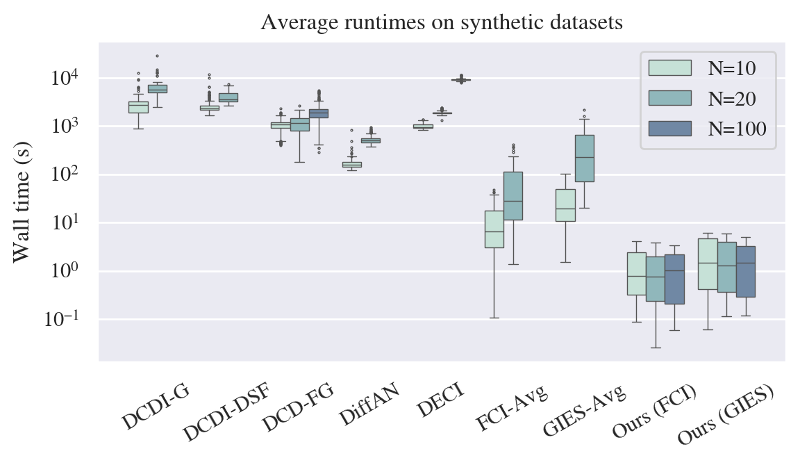
Figure 3: Average wall time required to run each model on a single dataset. The y-axis is plotted in log scale.

Sea excels across synthetic and realistic causal discovery tasks with fast runtimes. We also show that Sea performs well, even in low-data regimes. Additional results and ablations can be found in Appendix C, including classical algorithm hyperparameters, global statistics, and scaling to graphs much larger than those in the training set.

5.1 Synthetic experiments

Sea significantly outperforms the baselines across a variety of graph sizes and causal mechanisms in Table 3, and we maintain high performance even for causal mechanisms beyond the training set (Sigmoid, Polynomial). Our pretrained aggregator consistently improves upon the performance of its individual inputs (InvCov, Fci-Avg, Gies-Avg), demonstrating the value in learning such a model.

In terms of edge orientation accuracy, Sea outperforms the baselines in all settings (Table 4). We have omitted InvCov from this comparison since it does not orient edges.

Table 4: Synthetic experiments, edge direction accuracy (higher is better). All standard deviations were within $0.2$. The symbol $\dagger$ indicates that Sea was not pretrained on this setting.

$N$	$E$	Model	Linear	NN add	NN	Sig.†	Poly.†
10	10	Dcdi-G	$0.74$	$0.80$	$0.85$	$0.41$	$0.44$
		Dcdi-Dsf	$0.79$	$0.62$	$0.68$	$0.38$	$0.39$
		Dcd-Fg	$0.50$	$0.47$	$0.70$	$0.43$	$0.54$
		DiffAn	$0.61$	$0.55$	$0.26$	$0.53$	$0.47$
		Deci	$0.50$	$0.43$	$0.62$	$0.63$	$0.75$
		Fci-Avg	$0.52$	$0.43$	$0.41$	$0.55$	$0.40$
		Gies-Avg	$0.76$	$0.49$	$0.69$	$0.67$	$0.63$
		Sea (Fci)	$0.92$	0.92	0.94	$0.76$	$0.71$
		Sea (Gies)	0.94	$0.88$	$0.93$	0.84	0.79
20	80	Dcdi-G	$0.47$	$0.43$	$0.82$	$0.40$	$0.24$
		Dcdi-Dsf	$0.50$	$0.49$	$0.78$	$0.41$	$0.28$
		Dcd-Fg	$0.58$	$0.65$	$0.75$	$0.62$	$0.48$
		DiffAn	$0.46$	$0.28$	$0.36$	$0.45$	$0.21$
		Deci	$0.30$	$0.47$	$0.35$	$0.48$	$0.57$
		Fci-Avg	$0.19$	$0.19$	$0.22$	$0.33$	$0.23$
		Gies-Avg	$0.56$	$0.73$	$0.59$	$0.62$	$0.61$
		Sea (Fci)	0.93	0.90	0.93	0.85	0.89
		Sea (Gies)	$0.92$	$0.88$	$0.92$	$0.84$	0.89
100	400	Dcd-Fg	$0.46$	$0.60$	$0.70$	$0.67$	$0.53$
		Sea (Fci)	$0.93$	$0.90$	$0.91$	0.87	$0.82$
		Sea (Gies)	0.94	0.91	0.92	0.87	0.84

We benchmarked the runtimes of each algorithm over all test datasets of $N=10,20,100$, when possible (Figure 3). Our model is orders of magnitude faster than other continuous optimization methods. All deep learning models were run on a single V100-PCIE-32GB GPU, except for DiffAn, since we were unable to achieve consistent GPU and R support within a Docker environment using their codebase. For all models, we recorded only computation time (CPU and GPU) and omitted any file system-related time.

Table 5: Causal discovery on (real) Sachs dataset. While InvCov is a strong baseline for connectivity, it does not predict orientation. The relative performance of the methods depends on metric.

Model	mAP $\uparrow$	AUC $\uparrow$	SHD $\downarrow$	EdgeAcc $\uparrow$	Time (s) $\downarrow$
Dcdi-G	$0.17$	$0.55$	$21.0$	$0.20$	2436.5
Dcdi-Dsf	$0.20$	$0.59$	$20.0$	$0.20$	1979.6
Dcd-Fg	0.32	$0.59$	$27.0$	$0.35$	951.4
DiffAn	$0.14$	$0.45$	$37.0$	$0.41$	293.7
Deci	$0.21$	0.62	$28.0$	0.53	609.7
InvCov	$0.31$	$0.61$	$20.0$	—	0.002
Fci-Avg	$0.27$	$0.59$	$18.0$	$0.24$	41.9
Gies-Avg	$0.21$	$0.59$	$17.0$	$0.24$	77.9
Sea (Fci)	$0.23$	$0.54$	$24.0$	$0.47$	3.2
Sea (Gies)	$0.23$	$0.60$	14.0	$0.41$	2.9

5.2 Realistic experiments

We report results on the real Sachs protein dataset (Sachs et al., 2005) in Table 5. The relative performance of each model differs based on metric. Sea performs comparably, while maintaining fast inference speeds. However, despite the popularity of this dataset in causal discovery literature (due to lack of better alternatives), biological networks are known to be time-resolved and cyclic, so the validity of the ground truth “consensus” graph has been questioned by experts (Mooij et al., 2020).

We also trained a version of Sea (Fci) on 7200 synthetic mRNA datasets (Dibaeinia & Sinha, 2020), exceeding baselines across held-out test datasets (Appendix C.3).

5.3 Performance in low-data regimes

One of the main advantages of foundation models is that they enable high levels of performance in low resource scenarios. Figure 4 shows that Sea (Fci) only requires around $M=500$ data samples for decent performance on graphs with $N=100$ nodes. For these experiments, we set batch size $b=\min(500,M)$ and node subset size $k=5$. This is in contrast to existing continuous optimization methods, which require thousands to tens of thousands of samples to fit completely. Compared to the InvCov baseline estimated over the same number of points $b=M=500$ (dotted lines), Sea is able to perform significantly better.

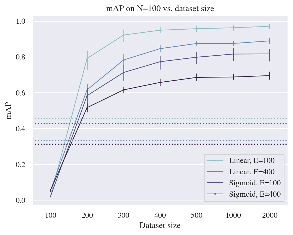
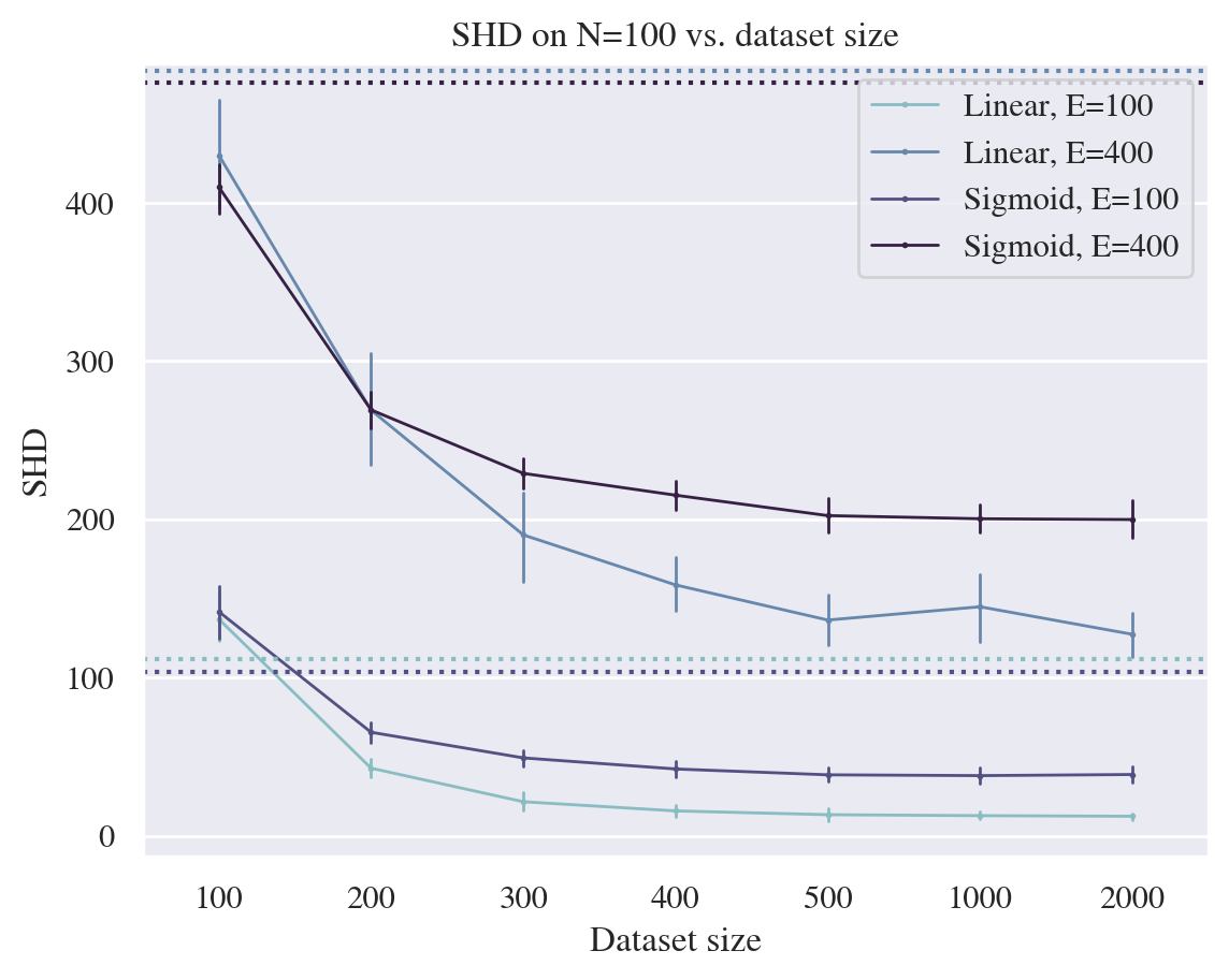
Figure 4: Performance of our model (FCI) as a function of total dataset size. Error bars indicate 95% confidence interval across the 5 datasets of each setting. Our model only requires approximately 500 samples for an acceptable level of performance on $N=100$ graphs. Dashed lines indicate the InvCov estimate on 500 points.

6 Conclusion

In this work, we introduced Sea, a framework for designing causal discovery foundation models. Sea is motivated by the idea that classical discovery algorithms provide powerful descriptors of data that are fast to compute and robust across datasets. Given these statistics, we train a deep learning model to reproduce faithful causal graphs. Theoretically, we demonstrated that it is possible to produce sound causal graphs from marginal estimates, and that our model has the capacity to do so. Empirically, we implemented two proofs of concept of Sea that perform well across a variety of causal discovery tasks. We hope that this work will inspire a new avenue of research in generalizable and scalable causal discovery algorithms.

7 Impact statement

This paper presents work whose goal is to advance the field of machine learning and causal inference. When applied to the biological sciences, these techniques may help uncover new knowledge regarding the interaction of genes and proteins. This information may then be used to develop both therapeutics and toxic substances. However, these techniques are only useful in the context of large-scale, high quality data, controlled access to which mitigates risk much more effectively than the restriction of any model discussed within this work.

Appendix A Proofs and derivations

Our theoretical contributions focus on two primary directions.

1. We formalize the notion of marginal estimates and prove that given sufficient marginal estimates, it is possible to recover a pattern faithful to the global causal graph. We provide lower bounds on the number of marginal estimates required for such a task, and motivate global statistics as an efficient means to reduce this bound.

2. We show that our proposed axial attention has the capacity to recapitulate the reasoning required for marginal estimate resolution. We provide realistic, finite bounds on the width and depth required for this task.

Before these formal discussions, we start with a toy example to provide intuition regarding marginal estimates and constraint-based causal discovery algorithms.

A.1 Toy example: Resolving marginal graphs

Consider the Y-shaped graph with four nodes in Figure 5. Suppose we run the PC algorithm on all subsets of three nodes, and we would like to recover the result of the PC algorithm on the full graph. We illustrate how one might resolve the marginal graph estimates. The PC algorithm consists of the following steps (Spirtes et al., 2001).

1. Start from the fully connected, undirected graph on $N$ nodes.

2. Remove all edges $(i,j)$ where $X_{i}\perp\!\!\!\perp X_{j}$.

3. For each edge $(i,j)$ and subsets $S\subseteq[N]\setminus\{i,j\}$ of increasing size $n=1,2,\dots,d$, where $d$ is the maximum degree in $G$, and all $k\in S$ are connected to either $i$ or $j$: if $X_{i}\perp\!\!\!\perp X_{j}\mid S$, remove edge $(i,j)$.

4. For each triplet $(i,j,k)$, such that only edges $(i,k)$ and $(j,k)$ remain, if $k$ was not in the set $S$ that eliminated edge $(i,j)$, then orient the “v-structure” as $i\rightarrow k\leftarrow j$.

5. (Orientation propagation) If $i\to j$, edge $(j,k)$ remains, and edge $(i,k)$ has been removed, orient $j\to k$. If there is a directed path $i\rightsquigarrow j$ and an undirected edge $(i,j)$, then orient $i\to j$.

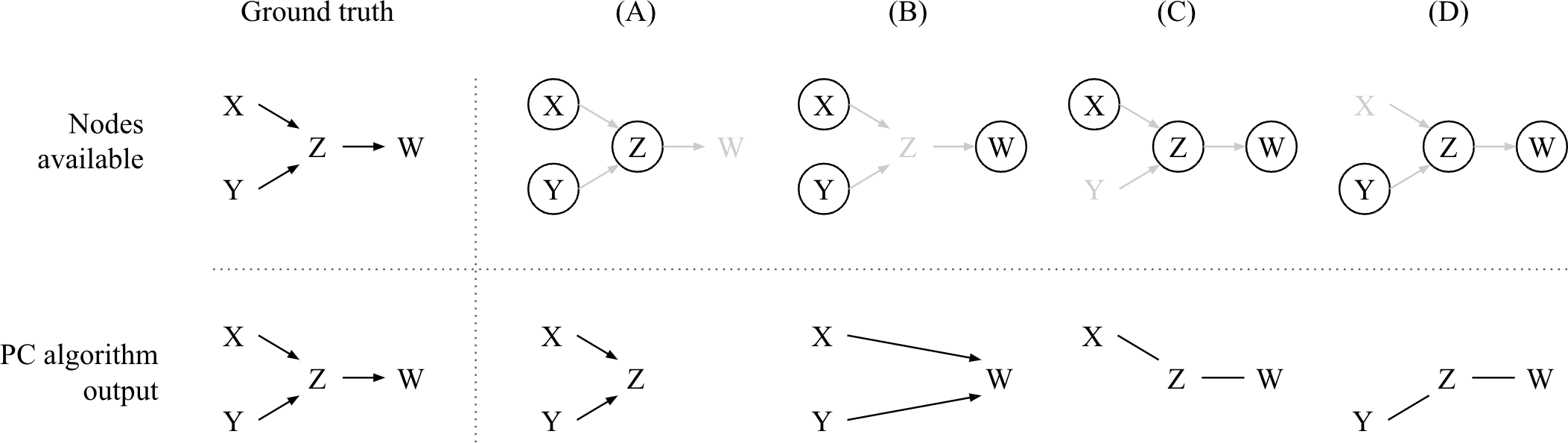
Figure 5: Resolving marginal graphs. Subsets of nodes revealed to the PC algorithm (circled in row 1) and its outputs (row 2).

In each of the four cases, the PC algorithm estimates the respective graphs as follows.

1. We remove edge $(X,Y)$ via (2) and orient the v-structure.

2. We remove edge $(X,Y)$ via (2) and orient the v-structure.

3. We remove edge $(X,W)$ via (3) by conditioning on $Z$. There are no v-structures, so the edges remain undirected.

4. We remove edge $(Y,W)$ via (3) by conditioning on $Z$. There are no v-structures, so the edges remain undirected.

The outputs (A-D) admit the full PC algorithm output as the only consistent graph on four nodes.

• $X$ and $Y$ are unconditionally independent, so no subset will reveal an edge between $(X,Y)$.

• There are no edges between $(X,W)$ and $(Y,W)$. Otherwise, (C) and (D) would yield the undirected triangle.

• $X,Y,Z$ must be oriented as $X\rightarrow Z\leftarrow Y$. Paths $X\to Z\to Y$ and $X\leftarrow Z\leftarrow Y$ would induce an $(X,Y)$ edge in (B). Reversing orientations $X\leftarrow Z\rightarrow Y$ would contradict (A).

• $(Y,Z)$ must be oriented as $Y\to Z$. Otherwise, (A) would remain unoriented.

A.2 Resolving marginal estimates into global graphs

A.2.1 Preliminaries

Classical results have characterized the Markov equivalency class of directed acyclic graphs. Two graphs are observationally equivalent if they have the same skeleton and v-structures (Verma & Pearl, 1990). Thus, a pattern $P$ is faithful to a graph $G$ if and only if they share the same skeletons and v-structures (Spirtes et al., 1990).

Definition A.1.

Let $G=(V,E)$ be a directed acyclic graph. A pattern $P$ is a set of directed and undirected edges over $V$.

Definition A.2 (Theorem 3.4 from Spirtes et al. (2001)).

If pattern $P$ is faithful to some directed acyclic graph, then $P$ is faithful to $G$ if and only if

1. for all vertices $X,Y$ of $G$, $X$ and $Y$ are adjacent if and only if $X$ and $Y$ are dependent conditional on every set of vertices of $G$ that does not include $X$ or $Y$; and

2. for all vertices $X,Y,Z$, such that $X$ is adjacent to $Y$ and $Y$ is adjacent to $Z$ and $X$ and $Z$ are not adjacent, $X\to Y\leftarrow Z$ is a subgraph of $G$ if and only if $X,Z$ are dependent conditional on every set containing $Y$ but not $X$ or $Z$.

Given data faithful to $G$, a number of classical constraint-based algorithms produce patterns that are faithful to $G$. We denote this set of algorithms as $\mathcal{F}$.

Theorem A.3 (Theorem 5.1 from (Spirtes et al., 2001)).

If the input to the PC, SGS, PC-1, PC-2, PC^∗, or IG algorithms faithful to directed acyclic graph $G$, the output is a pattern that represents the faithful indistinguishability class of $G$.

The algorithms in $\mathcal{F}$ are sound and complete if there are no unobserved confounders.

A.2.2 Marginal estimates

Let $P_{V}$ be a probability distribution that is Markov, minimal, and faithful to $G$. Let $D\in\mathbb{R}^{M\times N}\sim P_{V}$ be a dataset of $M$ observations over all $N=|V|$ nodes.

Consider a subset $S\subseteq V$. Let $D[S]$ denote the subset of $D$ over $S$,

$$D[S]=\{x_{i,v}:v\in S\}_{i=1}^{N},$$ (14)

and let $G[S]$ denote the subgraph of $G$ induced by $S$

$$G[S]=(S,\{(i,j):i,j\in S,(i,j)\in E\}.$$ (15)

If we apply any $f\in\mathcal{F}$ to $D[S]$, the results are not necessarily faithful to $G[S]$, as now there may be latent confounders in $V\setminus S$ (by construction). We introduce the term marginal estimate to denote the resultant pattern that, while not faithful to $G[S]$, is still informative.

Definition A.4 (Marginal estimate).

A pattern $E^{\prime}$ is a marginal estimate of $G[S]$ if and only if

1. for all vertices $X,Y$ of $S$, $X$ and $Y$ are adjacent if and only if $X$ and $Y$ are dependent conditional on every set of vertices of $S$ that does not include $X$ or $Y$; and

2. for all vertices $X,Y,Z$, such that $X$ is adjacent to $Y$ and $Y$ is adjacent to $Z$ and $X$ and $Z$ are not adjacent, $X\to Y\leftarrow Z$ is a subgraph of $S$ if and only if $X,Z$ are dependent conditional on every set containing $Y$ but not $X$ or $Z$.

A.2.3 Marginal estimate resolution

We claim that given marginal estimates on sufficient subsets of nodes, it is always possible to recover a pattern faithful to the entire graph. First we construct a mapping from marginal estimates to the desired pattern, and then we provide tighter bounds on the number of estimates required.

*

We will show that the following algorithm produces the desired answer. On a high level, lines 3-8 recover the undirected “skeleton” graph of $E^{*}$, lines 9-15 recover the v-structures, and line 16 references step 5 in Section A.1.

Algorithm 1 Resolve marginal estimates of $f\in\mathcal{F}$

1:  Input: Data $\mathcal{D}_{G}$ faithful to $G$

2:  Initialize $E^{\prime}\leftarrow K_{N}$ as the complete undirected graph on $N$ nodes.

3:  for $S\in\mathcal{S}_{d+2}$ do

4:     Compute $E^{\prime}_{S}=f(\mathcal{D}_{G[S]})$

5:     for $(i,j)\not\in E^{\prime}_{S}$ do

6:        Remove $(i,j)$ from $E^{\prime}$

7:     end for

8:  end for

9:  for $E^{\prime}_{S}\in\{E^{\prime}_{S}\}_{\mathcal{S}_{d+2}}$ do

10:     for v-structure $i\rightarrow j\leftarrow k$ in $E^{\prime}_{S}$ do

11:        if $\{i,j\},\{j,k\}\in E^{\prime}$ and $\{i,k\}\not\in E^{\prime}$ then

12:           Assign orientation $i\rightarrow j\leftarrow k$ in $E^{\prime}$

13:        end if

14:     end for

15:  end for

16:  Propagate orientations in $E^{\prime}$ (optional).

Remark A.5.

In the PC algorithm ((Spirtes et al., 2001), A.1), its derivatives, and Algorithm 1, there is no need to consider separating sets with cardinality greater than maximum degree $d$, since the maximum number of independence tests required to separate any node from the rest of the graph is equal to number of its parents plus its children (due to the Markov assumption).

Lemma A.6.

The undirected skeleton of $E^{*}$ is equivalent to the undirected skeleton of $E^{\prime}$

$$C^{*}\coloneqq\left\{\{i,j\}\mid(i,j)\in E^{*}\textrm{ or }(j,i)\in E^{*}\right\}=\left\{\{i,j\}\mid(i,j)\in E^{\prime}\textrm{ or }(j,i)\in E^{\prime}\right\}\coloneqq C^{\prime}.$$ (16)

That is, $\{i,j\}\in C^{*}\iff\{i,j\}\in C^{\prime}$.

Proof.

It is equivalent to show that $\{i,j\}\not\in C^{*}\iff\{i,j\}\not\in C^{\prime}$

$\Rightarrow$ If $\{i,j\}\not\in C*$, then there must exist a separating set $S$ in $G$ of at most size $d$ such that $i\perp\!\!\!\perp j\mid S$. Then $S\cup\{i,j\}$ is a set of at most size $d+2$, where $\{i,j\}\not\in C^{\prime}_{S\cup\{i,j\}}$. Thus, $\{i,j\}$ would have been removed from $C^{\prime}$ in line 6 of Algorithm 1.

$\Leftarrow$ If $\{i,j\}\not\in C^{\prime}$, let $S$ be a separating set in $\mathcal{S}_{d+2}$ such that $\{i,j\}\not\in C^{\prime}_{S\cup\{i,j\}}$ and $i\perp\!\!\!\perp j\mid S$. $S$ is also a separating set in $G$, and conditioning on $S$ removes $\{i,j\}$ from $C^{*}$. ∎

Lemma A.7.

A v-structure $i\rightarrow j\leftarrow k$ exists in $E^{*}$ if and only if there exists the same v-structure in $E^{\prime}$.

Proof.

The PCI algorithm orients v-structures $i\rightarrow j\leftarrow k$ in $E^{*}$ if there is an edge between $\{i,j\}$ and $\{j,k\}$ but not $\{i,k\}$; and if $j$ was not in the conditioning set that removed $\{i,k\}$. Algorithm 1 orients v-structures $i\rightarrow j\leftarrow k$ in $E^{\prime}$ if they are oriented as such in any $E^{\prime}_{S}$; and if $\{i,j\},\{j,k\}\in E^{\prime},\{i,k\}\not\in E^{\prime}$

$\Rightarrow$ Suppose for contradiction that $i\rightarrow j\leftarrow k$ is oriented as a v-structure in $E^{*}$, but not in $E^{\prime}$. There are two cases.

1. No $E^{\prime}_{S}$ contains the undirected path $i-j-k$. If either $i-j$ or $j-k$ are missing from any $E^{\prime}_{S}$, then $E^{*}$ would not contain $(i,j)$ or $(k,j)$. Otherwise, if all $S$ contain $\{i,k\}$, then $E^{*}$ would not be missing $\{i,k\}$ (Lemma A.6).

2. In every $E^{\prime}_{S}$ that contains $i-j-k$, $j$ is in the conditioning set that removed $\{i,k\}$, i.e. $i\perp\!\!\!\perp k\mid S,S\ni j$. This would violate the faithfulness property, as $j$ is neither a parent of $i$ or $k$ in $E^{*}$, and the outputs of the PC algorithm are faithful to the equivalence class of $G$ (Theorem 5.1 (Spirtes et al., 2001)).

$\Leftarrow$ Suppose for contradiction that $i\rightarrow j\leftarrow k$ is oriented as a v-structure in $E^{\prime}$, but not in $E^{*}$. By Lemma A.6, the path $i-j-k$ must exist in $E^{*}$. There are two cases.

1. If $i\to j\to k$ or $i\leftarrow j\leftarrow k$, then $j$ must be in the conditioning set that removes $\{i,k\}$, so no $E^{\prime}_{S}$ containing $\{i,j,k\}$ would orient them as v-structures.

2. If $j$ is the root of a fork $i\leftarrow j\rightarrow k$, then as the parent of both $i$ and $k$, $j$ must be in the conditioning set that removes $\{i,k\}$, so no $E^{\prime}_{S}$ containing $\{i,j,k\}$ would orient them as v-structures.

Therefore, all v-structures in $E^{\prime}$ are also v-structures in $E^{*}$. ∎

Proof of Theorem 3.4.

Given data that is faithful to $G$, Algorithm 1 produces a pattern $E^{\prime}$ with the same connectivity and v-structures as $E^{*}$. Any additional orientations in both patterns are propagated using identical, deterministic procedures, so $E^{\prime}=E^{*}$. ∎

This proof presents a deterministic but inefficient algorithm for resolving marginal subgraph estimates. In reality, it is possible to recover the undirected skeleton and the v-structures of $G$ without checking all subsets $S\in\mathcal{S}_{d+2}$.

*

Proof.

Following Lemma A.6, an edge $(i,j)$ is not present in $C$ if it is not present in any of the size $d+2$ estimates. Therefore, every pair of nodes $\{i,j\}$ requires only a single estimate of size $d+2$, so it is possible to recover $C$ in $\binom{N}{2}$ estimates. ∎

*

Proof.

Each v-structure $i\to j\leftarrow k$ falls under two cases.

1. $i\perp\!\!\!\perp k$ unconditionally. Then an estimate over $\{i,j,k\}$ will identify the v-structure.

2. $i\perp\!\!\!\perp k\mid S$, where $j\not\in S\subset V$. Then an estimate over $S\cup\{i,j,k\}$ will identify the v-structure. Note that $|S|\leq d+2$ since the degree of $i$ is at least $|S|+1$.

Therefore, each v-structure only requires one estimate, and it is possible to identify all v-structures in $O(\nu)$ estimates. ∎

There are three takeaways from this section.

1. If we exhaustively run a constraint-based algorithm on all subsets of size $d+2$, it is trivial to recover the estimate of the full graph. However, this is no more efficient than running the causal discovery algorithm on the full graph.

2. In theory, it is possible to recover the undirected graph in $O(N^{2})$ estimates, and the v-structures in $O(\nu)$ estimates. However, we may not know the appropriate subsets ahead of time.

3. In practice, if we have a surrogate for connectivity, such as the global statistics used in Sea, then we can vastly reduce the number of estimates used to eliminate edges from consideration, and more effectively focus on sampling subsets for orientation determination.

A.3 Computational power of the axial attention model

In this section, we focus on the computational capacity of our axial attention-based architecture. We show that three blocks can recover the skeleton and v-structures in $O(N)$ width, and additional blocks have the capacity to propagate orientations. We first formalize the notion of a neural network architecture’s capacity to “implement” an algorithm. Then we prove Theorem 3.4 by construction.

Definition A.8.

Let $f$ be a map from finite sets $Q$ to $F$, and let $\phi$ be a map from finite sets $Q_{\Phi}$ to $F_{\Phi}$. We say $\phi$ implements $f$ if there exists injection $g_{\textrm{in}}:Q\to Q_{\Phi}$ and surjection $g_{\textrm{out}}:F_{\Phi}\to F$ such that

$$\forall q\in Q,g_{\textrm{out}}(\phi(g_{\textrm{in}}(q)))=f(q).$$ (17)

Definition A.9.

Let $Q,F,Q_{\Phi},F_{\Phi}$ be finite sets. Let $f$ be a map from $Q$ to $F$, and let $\Phi$ be a finite set of maps $\{\phi:Q_{\Phi}\to F_{\Phi}\}$. We say $\Phi$ has the capacity to implement $f$ if and only if there exists at least one element $\phi\in\Phi$ that implements $f$.

*

Proof.

We consider axial attention blocks with dot-product attention and omit layer normalization from our analysis, as is common in the Transformer universality literature (Yun et al., 2019). Our inputs $X\in\mathbb{R}^{d\times R\times C}$ consist of $d$-dimension embeddings over $R$ rows and $C$ columns. Since our axial attention only operates over one dimension at a time, we use $X_{\cdot,c}$ to denote a 1D sequence of length $R$, given a fixed column $c$, and $X_{r,\cdot}$ to denote a 1D sequence of length $C$, given a fixed row $r$. A single axial attention layer (with one head) consists of two attention layers and a feedforward network,

$$\text{Attn}_{\text{row}}(X_{\cdot,c}) =X_{\cdot,c}+W_{O}W_{V}X_{\cdot,c}\cdot\sigma\left[(W_{K}X_{\cdot,c})^{T}W_{Q}X_{\cdot,c}\right],$$ (18)

$$X \leftarrow\text{Attn}_{\text{row}}(X)$$

$$\text{Attn}_{\text{col}}(X_{r,\cdot}) =X_{r,\cdot}+W_{O}W_{V}X_{r,\cdot}\cdot\sigma\left[(W_{K}X_{r,\cdot})^{T}W_{Q}X_{r,\cdot}\right],$$ (19)

$$X \leftarrow\text{Attn}_{\text{col}}(X)$$

$$\text{FFN}(X) =X+W_{2}\cdot\text{ReLU}(W_{1}\cdot X+b_{1}\mathbf{1}_{L}^{T})+b_{2}\mathbf{1}_{L}^{T},$$ (20)

where $W_{O}\in\mathbb{R}^{d\times d},W_{V},W_{K},W_{Q}\in\mathbb{R}^{d\times d},W_{2}\in\mathbb{R}^{d\times m},W_{1}\in\mathbb{R}^{m\times d},b_{2}\in\mathbb{R}^{d},b_{1}\in\mathbb{R}^{m}$, and $m$ is the hidden layer size of the feedforward network. For concision, we have omitted the $r$ and $c$ subscripts on the $W$s, but the row and column attentions use different parameters. Any row or column attention can take on the identity mapping by setting $W_{O},W_{V},W_{K},W_{Q}$ to $d\times d$ matrices of zeros.

A single axial attention block consists of two axial attention layers $\phi_{E}$ and $\phi_{\rho}$, connected via messages (Section 3.2)

$$h^{E,\ell} =\phi_{E,\ell}(h^{E,\ell-1})$$

$$h^{\rho,\ell-1} \leftarrow W_{\rho,\ell}\left[h^{\rho,\ell-1},m^{E\to\rho,\ell}\right]$$

$$h^{\rho,\ell} =\phi_{\rho,\ell}(h^{\rho,\ell-1})$$

$$h^{E,\ell} \leftarrow h^{E,\ell}+m^{\rho\to E,\ell}$$

where $h^{\ell}$ denote the hidden representations of $E$ and $\rho$ at layer $\ell$, and the outputs of the axial attention block are $h^{\rho,\ell},h^{E,\ell}$.

We construct a stack of $L\geq 3$ axial attention blocks that implement Algorithm 1.

Model inputs

Consider edge estimate $E^{\prime}_{i,j}\in\mathcal{E}$ in a graph of size $N$. Let $e_{i},e_{j}$ denote the endpoints of $(i,j)$. Outputs of the PC algorithm can be expressed by three endpoints: $\{\varnothing,\bullet,\blacktriangleright\}$. A directed edge from $i\to j$ has endpoints $(\bullet,\blacktriangleright)$, the reversed edge $i\leftarrow j$ has endpoints $(\blacktriangleright,\bullet)$, an undirected edge has endpoints $(\bullet,\bullet)$, and the lack of any edge between $i,j$ has endpoints $(\varnothing,\varnothing)$.

Let $\textrm{one-hot}_{N}(i)$ denote the $N$-dimensional one-hot column vector where element $i$ is 1. We define the embedding of $(i,j)$ as a $d=2N+6$ dimensional vector,

$$g_{\text{in}}(E_{t,(i,j)})=h^{E,0}_{(i,j)}=\left[\begin{array}[]{c}\textrm{one-hot}_{3}(e_{i})\\ \hline\cr\textrm{one-hot}_{3}(e_{j})\\ \hline\cr\textrm{one-hot}_{N}(i)\\ \hline\cr\textrm{one-hot}_{N}(j)\end{array}\right].$$ (21)

To recover graph structures from $h^{E}$, we simply read off the indices of non-zero entries ($g_{\text{out}}$). We can set $h^{\rho,0}$ to any $\mathbb{R}^{d\times N\times N}$ matrix, as we do not consider its values in this analysis and discard it during the first step.

Claim A.10.

(Consistency) The outputs of each step

1. are consistent with (21), and

2. are equivariant to the ordering of nodes in edges.

For example, if $(i,j)$ is oriented as $(\blacktriangleright,\bullet)$, then we expect $(j,i)$ to be oriented $(\bullet,\blacktriangleright)$.

Step 1: Undirected skeleton

We use the first axial attention block to recover the undirected skeleton $C^{\prime}$. We set all attentions to the identity, set $W_{\rho,1}\in\mathbb{R}^{2d\times d}$ to a $d\times d$ zeros matrix, stacked on top of a $d\times d$ identity matrix (discard $\rho$), and set $\text{FFN}_{E}$ to the identity (inputs are positive). This yields

$$h^{\rho,0}_{i,j}=m^{E\to\rho,1}_{i,j}=\left[\begin{array}[]{c}P_{e_{i}}(\varnothing)\\ P_{e_{i}}(\bullet)\\ P_{e_{i}}(\blacktriangleright)\\ \hline\cr\vdots\\ \hline\cr\textrm{one-hot}_{N}(i)\\ \hline\cr\textrm{one-hot}_{N}(j)\end{array}\right],$$ (22)

where $P_{e_{i}}(\cdot)$ is the frequency that endpoint $e_{i}=\cdot$ within the subsets sampled. FFNs with 1 hidden layer are universal approximators of continuous functions (Hornik et al., 1989), so we use $\text{FFN}_{\rho}$ to map

$$\text{FFN}_{\rho}(X_{i,u,v})=\begin{cases}0&i\leq 6\\ 0&i>6,X_{1,u,v}=0\\ -X_{i,u,v}&\text{ otherwise,}\end{cases}$$ (23)

where $i\in[2N+6]$ indexes into the feature dimension, and $u,v$ index into the rows and columns. This allows us to remove edges not present in $C^{\prime}$ from consideration:

$$m^{\rho\to E,1} =h^{\rho,1}$$

$$h^{E,1}_{i,j} \leftarrow h^{E,1}_{i,j}+m^{\rho\to E,1}_{i,j}=\begin{cases}0&(i,j)\not\in C^{\prime}\\ h^{E,0}_{i,j}&\text{ otherwise.}\end{cases}$$ (24)

This yields $(i,j)\in C^{\prime}$ if and only if $h^{\rho,1}_{i,j}\neq\mathbf{0}$. We satisfy A.10 since our inputs are valid PC algorithm outputs for which $P_{e_{i}}(\varnothing)=P_{e_{j}}(\varnothing)$.

Step 2: V-structures

The second and third axial attention blocks recover v-structures. We run the same procedure twice, once to capture v-structures that point towards the first node in an ordered pair, and one to capture v-structures that point towards the latter node.

We start with the first row attention over edge estimates, given a fixed subset $t$. We set the key and query attention matrices

$$W_{K}=k\cdot\left[\begin{array}[]{rrrrrrrr}0&0&1\\ &&&0&1&0\\ &\vdots\\ &&&&&&I_{N}\\ &&&&&&&-I_{N}\end{array}\right] W_{Q}=k\cdot\left[\begin{array}[]{rrrrrrrr}0&0&1\\ &&&0&1&0\\ &\vdots\\ &&&&&&I_{N}\\ &&&&&&&I_{N}\end{array}\right]$$ (35)

where $k$ is a large constant, $I_{N}$ denotes the size $N$ identity matrix, and all unmarked entries are 0s.

Recall that a v-structure is a pair of directed edges that share a target node. We claim that two edges $(i,j),(u,v)$ form a v-structure in $E^{\prime}$, pointing towards $i=u$, if this inner product takes on the maximum value

$$\left\langle(W_{K}h^{E,1})_{i,j},(W_{Q}h^{E,1})_{u,v}\right\rangle=3.$$ (36)

Suppose both edges $(i,j)$ and $(u,v)$ still remain in $C^{\prime}$. There are two components to consider.

1. If $i=u$, then their shared node contributes $+1$ to the inner product (prior to scaling by $k$). If $j=v$, then the inner product accrues $-1$.

2. Nodes that do not share the same endpoint contribute 0 to the inner product. Of edges that share one node, only endpoints that match $\blacktriangleright$ at the starting node, or $\bullet$ at the ending node contribute $+1$ to the inner product each. We provide some examples below.

   $(e_{i},e_{j})$	$(e_{u},e_{v})$	contribution	note
   $(\blacktriangleright,\bullet)$	$(\bullet,\blacktriangleright)$	$0$	no shared node
   $(\bullet,\blacktriangleright)$	$(\bullet,\blacktriangleright)$	$0$	wrong endpoints
   $(\bullet,\bullet)$	$(\bullet,\bullet)$	$1$	one correct endpoint
   $(\blacktriangleright,\bullet)$	$(\blacktriangleright,\bullet)$	$2$	v-structure

All edges with endpoints $\varnothing$ were “removed” in step 1, resulting in an inner product of zero, since their node embeddings were set to zero. We set $k$ to some large constant (empirically, $k^{2}=1000$ is more than enough) to ensure that after softmax scaling, $\sigma_{e,e^{\prime}}>0$ only if $e,e^{\prime}$ form a v-structure.

Given ordered pair $e=(i,j)$, let $V_{i}\subset V$ denote the set of nodes that form a v-structure with $e$ with shared node $i$. Note that $V_{i}$ excludes $j$ itself, since setting of $W_{K},W_{Q}$ exclude edges that share both nodes. We set $W_{V}$ to the identity, and we multiply by attention weights $\sigma$ to obtain

$$(W_{V}h^{E,1}\sigma)_{e=(i,j)}=\left[\begin{array}[]{c}\vdots\\ \hline\cr\text{one-hot}_{N}(i)\\ \hline\cr\alpha_{j}\cdot\text{binary}_{N}(V_{j})\end{array}\right]$$ (37)

where $\text{binary}_{N}(S)$ denotes the $N$-dimensional binary vector with ones at elements in $S$, and the scaling factor

$$\alpha_{j}=(1/\|V_{j}\|)\cdot\mathbbm{1}\{\|V_{j}\|>0\}\in[0,1]$$ (38)

results from softmax normalization. We set

$$W_{O}=\left[\begin{array}[]{rr}\mathbf{0}_{N+6}\\ &0.5\cdot I_{N}\end{array}\right]$$ (39)

to preserve the original endpoint values, and to distinguish between the edge’s own node identity and newly recognized v-structures. To summarize, the output of this row attention layer is

$$\text{Attn}_{\text{row}}(X_{\cdot,c})=X_{\cdot,c}+W_{O}W_{V}X_{\cdot,c}\cdot\sigma,$$

which is equal to its input $h^{E,1}$ plus additional positive values $\in(0,0.5)$ in the last $N$ positions that indicate the presence of v-structures that exist in the overall $E^{\prime}$.

Our final step is to “copy” newly assigned edge directions into all the edges. We set the $\phi_{E}$ column attention, $\text{FFN}_{E}$ and the $\phi_{\rho}$ attentions to the identity mapping. We also set $W_{\rho,2}$ to a $d\times d$ zeros matrix, stacked on top of a $d\times d$ identity matrix. This passes the output of the $\phi_{E}$ row attention, aggregated over subsets, directly to $\text{FFN}_{\phi,2}$.

For endpoint dimensions $\mathbf{e}=[6]$, we let $\text{FFN}_{\phi,2}$ implement

$$\text{FFN}_{\rho,2}(X_{\mathbf{e},u,v})=\begin{cases}[0,0,1,0,1,0]^{T}-X_{\mathbf{e},u,v}&0<\sum_{i>N+6}X_{i,u,v}<0.5\\ 0&\text{ otherwise.}\end{cases}$$ (40)

Subtracting $X_{\mathbf{e},u,v}$ “erases” the original endpoints and replaces them with $(\blacktriangleright,\bullet)$ after the update

$$h^{E,1}_{i,j}\leftarrow h^{E,1}_{i,j}+m^{\rho\to E,1}_{i,j}.$$

The overall operation translates to checking whether any v-structure points towards $i$, and if so, assigning edge directions accordingly. For dimensions $i>6$,

$$\text{FFN}_{\rho,2}(X_{i,u,v})=\begin{cases}-X_{i,u,v}&X_{i,u,v}\leq 0.5\\ 0&\text{ otherwise,}\end{cases}$$ (41)

effectively erasing the stored v-structures from the representation and remaining consistent to (21).

At this point, we have copied all v-structures once. However, our orientations are not necessarily symmetric. For example, given v-structure $i\to j\leftarrow k$, our model orients edges $(j,i)$ and $(j,k)$, but not $(i,j)$ or $(k,j)$.

The simplest way to symmetrize these edges (for the writer and the reader) is to run another axial attention block, in which we focus on v-structures that point towards the second node of a pair. The only changes are as follows.

• For $W_{K}$ and $W_{Q}$, we swap columns 1-3 with 4-6, and columns 7 to $N+6$ with the last $N$ columns.

• $(h^{E,2}\sigma)_{i,j}$ sees the third and fourth blocks swapped.

• $W_{O}$ swaps the $N\times N$ blocks that correspond to $i$ and $j$’s node embeddings.

• $\text{FFN}_{\rho,3}$ sets the endpoint embedding to $[0,1,0,0,0,1]^{T}-X_{\mathbf{e},u,v}$ if $i=7,...,N+6$ sum to a value between 0 and 0.5.

The result is $h^{E,3}$ with all v-structures oriented symmetrically, satisfying A.10.

Step 3: Orientation propagation

To propagate orientations, we would like to identify cases $(i,j),(i,k)\in E^{\prime},(j,k)\not\in E^{\prime}$ with shared node $i$ and corresponding endpoints $(\blacktriangleright,\bullet),(\bullet,\bullet)$. We use $\phi_{E}$ to identify triangles, and $\phi_{\rho}$ to identify edges $(i,j),(i,k)\in E^{\prime}$ with the desired endpoints, while ignoring triangles.

Marginal layer

The row attention in $\phi_{E}$ fixes a subset $t$ and varies the edge $(i,j)$.

Given edge $(i,j)$, we want to extract all $(i,k)$ that share node $i$. We set the key and query attention matrices to

$$W_{K},W_{Q}=k\cdot\left[\begin{array}[]{rrrrrrrr}0&1&1&0&1&1\\ \vdots\\ &&&&&&I_{N}\\ &&&&&&&\pm I_{N}\\ \end{array}\right].$$ (42)

We set $W_{V}$ to the identity to obtain

$$(W_{V}h^{E}\sigma)_{e=(i,k)}=\left[\begin{array}[]{c}\vdots\\ \hline\cr\vdots\\ \hline\cr\text{one-hot}_{N}(i)\\ \hline\cr\alpha_{k}\cdot\text{binary}_{N}(V_{k})\end{array}\right],$$ (43)

where $V_{k}$ is the set of nodes $k$ that share any edge with $i$. To distinguish between $k$ and $V_{k}$, we again set $W_{o}$ to the same as in (39). Finally, we set $\text{FFN}_{E}$ to the identity and pass $h^{E}$ directly to $\phi_{\rho}$. To summarize, we have $h^{E}$ equal to its input, with values $\in(0,0.5)$ in the last $N$ locations indicating 1-hop neighbors of each edge.

Global layer

Now we would like to identify cases $(i,k),(j,k)$ with corresponding endpoints $(\bullet,\blacktriangleright),(\bullet,\bullet)$. We set the key and query attention matrices

$$W_{K}=k\cdot\left[\begin{array}[]{rrrrr}0&0&1\\ \vdots\\ &&&I_{N}\\ &&&&I_{N}\end{array}\right] W_{Q}=k\cdot\left[\begin{array}[]{rrrrrrrr}0&1&-1&0&1&-1\\ \vdots\\ &&&&&&I_{N}\\ &&&&&&&-I_{N}\end{array}\right].$$ (52)

The key allows us to check that endpoint $i$ is directed, and the query allows us to check that $(i,k)$ exists in $C^{\prime}$, and does not already point elsewhere. After softmax normalization, for sufficiently large $k$, we obtain $\sigma_{(i,j),(i,k)}>0$ if and only if $(i,k)$ should be oriented $(\bullet,\blacktriangleright)$, and the inner product attains the maximum possible value

$$\left\langle(W_{K}h^{\rho})_{i,j},(W_{Q}h^{\rho})_{i,k}\right\rangle=2.$$ (53)

We consider two components.

1. If the endpoints match our desired endpoints, we gain a $+1$ contribution to the inner product.

2. A match between the first nodes contributes $+1$. If the second node shares any overlap (either same edge, or a triangle), then a negative value would be added to the overall inner product.

Therefore, we can only attain the maximal inner product if only one edge is directed, and if there exists no triangle.

We set $W_{o}$ to the same as in (39), and we add $h^{\rho}$ to the input of the next $\phi_{E}$. To summarize, we have $h^{\rho}$ equal to its input, with values $\in(0,0.5)$ in the last $N$ locations indicating incoming edges.

Orientation assignment

Our final step is to assign our new edge orientations. Let the column attention take on the identity mapping. For endpoint dimensions $\mathbf{e}=(4,5,6)$, we let $\text{FFN}_{\rho}$ implement

$$\text{FFN}_{\rho}(X_{\mathbf{e},u,v})=\begin{cases}[0,0,1]^{T}-X_{\mathbf{e},u,v}&0<\sum_{i>N+6}X_{i,u,v}<0.5\\ 0&\text{ otherwise.}\end{cases}$$ (54)

This translates to checking whether any incoming edge points towards $v$, and if so, assigning the new edge direction accordingly. For dimensions $i>6$,

$$\text{FFN}_{\rho}(X_{i,u,v})=\begin{cases}0&X_{i,u,v}\leq 0.5\\ X_{i,u,v}&\text{ otherwise,}\end{cases}$$ (55)

effectively erasing the stored assignments from the representation. Thus, we are left with $h^{E,\ell}$ that conforms to the same format as the initial embedding in (21).

To symmetrize these edges, we run another axial attention block, in which we focus on paths that point towards the second node of a pair. The only changes are as follows.

• For $\phi_{E}$ layer $W_{K}$ and $W_{Q}$ (42), we swap $I_{N}$ and $\pm I_{N}$.

• For $\phi_{\rho}$ layer $W_{K}$ and $W_{Q}$ (52), we swap $I_{N}$ and $\pm I_{N}$.

• $W_{O}$ swaps the $N\times N$ blocks that correspond to $i$ and $j$’s node embeddings.

• For $\text{FFN}_{\rho}$ (54), we let $\mathbf{e}=(1,2,3)$ instead.

The result is $h^{E}$ with symmetric 1-hop orientation propagation, satisfying A.10. We may repeat this procedure $k$ times to capture $k$-hop paths.

To summarize, we used axial attention block 1 to recover the undirected skeleton $C^{\prime}$, blocks 2-3 to identify and copy v-structures in $E^{\prime}$, and all subsequent $L-3$ layers to propagate orientations on paths up to $\lfloor(L-3)/2\rfloor$ length. Overall, this particular construction requires $O(N)$ width for $O(L)$ paths.

∎

Final remarks

Information theoretically, it should be possible to encode the same information in $\log N$ space, and achieve $O(\log N)$ width. For ease of construction, we have allowed for wider networks than optimal.

On the other hand, if we increase the width and encode each edge symmetrically, e.g. $(e_{i},e_{j},e_{j},e_{i}\mid i,j,j,i)$, we can reduce the number of blocks by half, since we no longer need to run each operation twice. However, attention weights scale quadratically, so we opted for an asymmetric construction.

Finally, a strict limitation of our model is that it only considers 1D pairwise interactions. In the graph layer, we cannot compare different edges’ estimates at different times in a single step. In the feature layer, we cannot compare $(i,j)$ to $(j,i)$ in a single step either. However, the graph layer does enable us to compare all edges at once (sparsely), and the feature layer looks at a time-collapsed version of the whole graph. Therefore, though we opted for this design for computational efficiency, we have shown that it is able to capture significant graph reasoning.

A.4 Robustness and stability

We discuss the notion of stability informally, in the context of Spirtes et al. (2001). There are two cases in which our framework may receive erroneous inputs: low/noisy data settings, and functionally misspecified situations. We consider our framework’s robustness to these cases, in terms of recovering the skeleton and orienting edges.

A.4.1 Data noise

In the case of noisy data, edges may be erroneously added, removed, or misdirected from marginal estimates $E^{\prime}$. Our framework provides two avenues to mitigating such noise.

1. We observe that global statistics can be estimated reliably in low data scenarios. For example, Figure 6 suggests that 200 examples suffice to provide a robust estimate over 100 variables in our synthetic settings. Therefore, even if the marginal estimates are erroneous, the neural network can learn the skeleton from the global statistics.

2. Most classical causal discovery algorithms are not stable with respect to edge orientation assignment. That is, an error in a single edge may propagate throughout the graph. Empirically, we observe that the majority vote of Gies achieves reasonable accuracy even without any training, while Fci suffers in this assessment (Table 4). However both Sea (Gies) and Sea (Fci) achieve high edge accuracy. Therefore, while the underlying algorithms may not be stable with respect to edge orientation, our pretrained aggregator seems to be robust.

A.4.2 Functional misspecification

It is also possible that our global statistics and marginal estimates make misspecified assumptions regarding the data generating mechanisms. The degree of misspecification can vary case by case, so it is hard to provide any broad guarantees about the performance of our algorithm, in general. However, we can make the following observation.

If two variables are independent, $X_{i}\perp\!\!\!\perp X_{j}$, they are independent, e.g. under linear Gaussian assumptions. If $X_{i},X_{j}$ exhibit more complex functional dependencies, they may be erroneously deemed independent. Therefore, any systematic errors are necessarily one-sided, and the model can learn to recover the connectivity based on global statistics.

Appendix B Experimental details

B.1 Synthetic data generation

Synthetic datasets were generated using code from Dcdi (Brouillard et al., 2020), which extended the Causal Discovery Toolkit data generators to interventional data (Kalainathan et al., 2020).

We considered the following causal mechanisms. Let $y$ be the node in question, let $X$ be its parents, let $E$ be an independent noise variable (details below), and let $W$ be randomly initialized weight matrices.

• Linear: $y=XW+E$.

• Polynomial: $y=W_{0}+XW_{1}+X^{2}W_{2}+E$

• Sigmoid additive: $y=\sum_{i=1}^{d}W_{i}\cdot\text{sigmoid}(X_{i})+E$

• Randomly initialized neural network (NN): $y=\text{Tanh}((X,E)W_{\text{in}})W_{\text{out}}$

• Randomly initialized neural network, additive (NN additive): $y=\text{Tanh}(XW_{\text{in}})W_{\text{out}}+E$

Root causal mechanisms, noise variables, and interventional distributions maintained the Dcdi defaults.

• Root causal mechanisms were set to $\text{Uniform}(-2,2)$.

• Noise was set to $E\sim 0.4\cdot\mathcal{N}(0,\sigma^{2})$ where $\sigma^{2}\sim\text{Uniform}(1,2)$.

• Interventions were applied to all nodes (one at a time) by setting their causal mechanisms to $\mathcal{N}(0,1)$.

Ablation datasets with $N>100$ nodes contained 100,000 points each (same as $N=100$).

B.2 Baseline details

We considered the following baselines. All baselines were run using official implementations published by the authors.

Dcdi (Brouillard et al., 2020) was trained on each of the $N=10,20$ datasets using their published hyperparameters. We denote the Gaussian and Deep Sigmoidal Flow versions as Dcdi-G and Dcdi-Dsf respectively. Dcdi could not scale to graphs with $N=100$ due to memory constraints (did not fit on a 32GB V100 GPU).

Dcd-Fg (Lopez et al., 2022) was trained on all of the test datasets using their published hyperparameters. We set the number of factors to $5,10,20$ for each of $N=10,20,100$, based on their ablation studies. Due to numerical instability on $N=100$, we clamped augmented Lagrangian multipliers $\mu$ and $\gamma$ to 10 and stopped training if elements of the learned adjacency matrix reached NaN values. After discussion with the authors, we also tried adjusting the $\mu$ multiplier from 2 to 1.1, but the model did not converge within 48 hours.

Deci (Geffner et al., 2022) was trained on all of the test datasets using their published hyperparameters. However, on all $N=100$ cases, the model failed to produce any meaningful results (adjacency matrices nearly all remained 0s with AUCs of 0.5). Thus, we only report results on $N=10,20$.

DiffAN (Sanchez et al., 2023) was trained on the each of the $N=10,20$ datasets using their published hyperparameters. The authors write that “most hyperparameters are hard-coded into [the] constructor of the DiffAN class and we verified they work across a wide set of datasets.” We used the original, non-approximation version of their algorithm by maintaining residue=True in their codebase. We were unable to consistently run DiffAN with both R and GPU support within a Docker container, and the authors did not respond to questions regarding reproducibility, so all models were trained on the CPU only. We observed approximately a 10x speedup in the $<5$ cases that were able to complete running on the GPU.

B.3 Neural network design

Hyperparameters and architectural choices were selected by training the model on 20% of the the training and validation data for approximately 50k steps (several hours). We considered the following parameters in sequence.

• learned positional embedding vs. sinusoidal positional embedding

• number of layers $\times$ number of heads: $\{4,8\}\times\{4,8\}$

• learning rate $\eta=\{1e-4,5e-5,1e-5\}$

For our final model, we selected learned positional embeddings, 4 layers, 8 heads, and learning rate $\eta=1e-4$.

B.4 Training and hardware details

The models were trained across 2 NVIDIA RTX A6000 GPUs and 60 CPU cores. We used the GPU exclusively for running the aggregator, and retained all classical algorithm execution on the CPUs (during data loading). The total pretraining time took approximately 14 hours for the final FCI model and 16 hours for the final GIES model.

For the scope of this paper, our models and datasets are fairly small. We did not scale further due to hardware constraints. Our primary bottlenecks to scaling up lay in availability of CPU cores and networking speed across nodes, rather than GPU memory or utilization.

We are able to run inference comfortably over $N=500$ graphs with $T=500$ subsets of $k=5$ nodes each, on a single 32GB V100 GPU. For runtime analysis, we used a batch size of 1, with 1 data worker per dataset. Runtime could be further improved if we amortized the GPU utilization across batches.

B.5 Choice of classical causal discovery algorithm

We selected FCI (Spirtes et al., 1995) as the underlying discovery algorithm in the observational setting over GES (Chickering, 2002) and GRaSP (Lam et al., 2022) due to its superior downstream performance. We hypothesize this may be due to its richer output (ancestral graph) providing more signal to the Transformer model. We also tried Causal Additive Models (Bühlmann et al., 2014), but its runtime was too slow for consistent GPU utilization. Observational algorithm implementations were provided by the causal-learn library (Zheng et al., 2023). The code for running these alternative classical algorithms is available in our codebase.

We selected GIES as the underlying discovery algorithm in the interventional setting because a Python implementation was readily available at https://github.com/juangamella/gies.

We tried incorporating implementations from the Causal Discovery Toolbox via a Docker image (Kalainathan et al., 2020), but there was excessive overhead associated with calling an R subroutine and reading/writing the inputs/results from disk.

Finally, we considered other independence tests for richer characterization, such as kernel-based methods. However, due to speed, we chose to remain with the default Fisherz conditional independence test for FCI, and BIC for GIES (Schwarz, 1978).

B.6 Sampling procedure

Selection scores:

We consider three strategies for computing selection scores $\alpha$. We include an empirical comparison of these strategies in Table 9.

1. Random selection: $\alpha$ is an $N\times N$ matrix of ones.

2. Global-statistic-based selection: $\alpha=\rho$.

3. Uncertainty-based selection: $\alpha=\hat{H}(E_{t}$), where $H$ denotes the information entropy

   $$\alpha_{i,j}=-\sum_{e\in\{0,1,2\}}p(e)\log p(e).$$ (56)

Let $c_{i,j}^{t}$ be the number of times edge $(i,j)$ was selected in $S_{1}\dots S_{t-1}$, and let $\alpha^{t}=\alpha/\sqrt{c_{i,j}^{t}}$. We consider two strategies for selecting $S_{t}$ based on $\alpha_{t}$.

Greedy selection:

Throughout our experiments, we used a greedy algorithm for subset selection. We normalize probabilities to 1 before the constructing each Categorical. Initialize

$$S_{t}\leftarrow\{i:i\sim\text{Categorical}(\alpha_{1}^{t}\dots\alpha_{N}^{t})\}.$$ (57)

where $\alpha_{i}^{t}=\sum_{j\neq i\in V}\alpha_{i,j}^{t}$. While $\lvert S_{t}\rvert<k$, update

$$S_{t}\leftarrow S_{t}\cup\{j:j\sim\text{Categorical}(\alpha_{1,S_{t}}^{t}\dots\alpha_{N,S_{t}}^{t}))$$ (58)

where

$$\alpha_{j,S_{t}}=\begin{cases}\sum_{i\in S_{t}}\alpha_{i,j}^{t}&j\not\in S_{t}\\ 0&\text{otherwise}.\end{cases}$$ (59)

Subset selection:

We also considered the following subset-level selection procedure, and observed minor performance gain for significantly longer runtime (linear program takes around 1 second per batch). Therefore, we opted for the greedy method instead.

We solve the following integer linear program to select a subset $S_{t}$ of size $k$ that maximizes $\sum_{i\in S_{t}}\alpha_{i,j}^{t}$. Let $\nu_{i}\in\{0,1\}$ denote the selection of node $i$, and let $\epsilon_{i,j}\in\{0,1\}$ denote the selection of edge $(i,j)$. Our objective is to

$$\begin{array}[]{ll@{}ll}\text{maximize}&\sum_{i,j}a_{i,j}^{t}\cdot\epsilon_{i,j}&\\ \text{subject to}&\sum_{i}\nu_{i}=k&\text{ \small subset size}\\ &\epsilon_{i,j}\geq\nu_{i}+\nu_{j}-1&\text{ \small node-edge consistency}\\ &\epsilon_{i,j}\leq\nu_{i}\\ &\epsilon_{i,j}\leq\nu_{j},\\ &\nu_{i}\in\{0,1\}\\ &\epsilon_{i,j}\in\{0,1\}\end{array}$$

for $i,j\in V\times V$, $i\in V$. $S_{t}$ is the set of non-zero indices in $\nu$.

The final algorithm used the greedy selection strategy, with the first half of batches sampled according to global statistics, and the latter half sampled randomly, with visit counts shared. This strategy was selected heuristically, and we did not observe significant improvements or drops in performance when switching to other strategies (e.g. all greedy statistics-based, greedy uncertainty-based, linear program uncertainty-based, etc.)

Appendix C Additional analyses

C.1 Traditional algorithm parameters

We investigated model performance with respect to the settings of our graph estimation parameters. Our model is sensitive to the size of batches used to estimate global features and marginal graphs (Figure 6). In particular, at least 250 points are required per batch for an acceptable level of performance. Our model is not particularly sensitive to the number of batches sampled (Figure 7), or to the number of variables sampled in each subset (Figure 8).

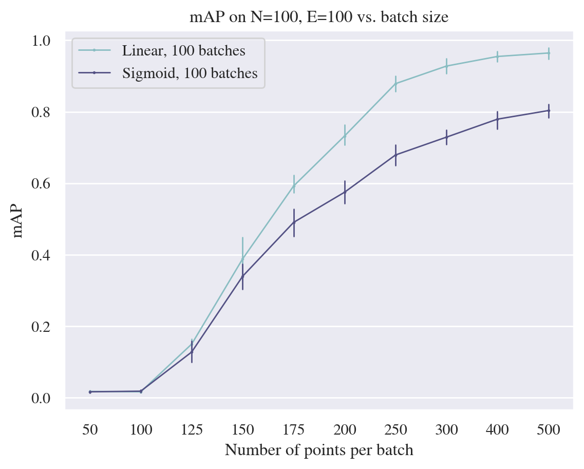
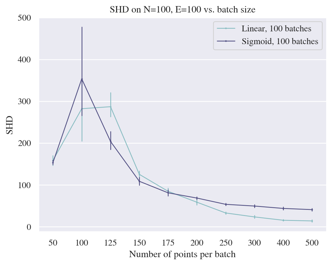
Figure 6: Performance of our model (GIES) as a function of traditional algorithm batch size. Error bars indicate 95% confidence interval across the 10 datasets of each setting. The global feature and marginal graph estimates are sensitive to batch size and require at least 250 points per batch to achieve an acceptable level of performance.

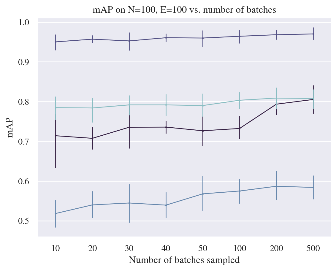
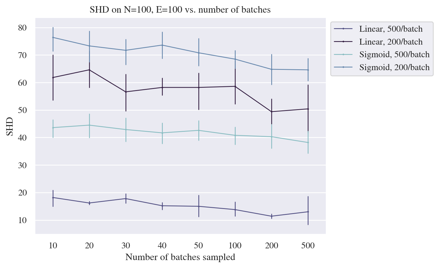
Figure 7: Performance of our model (GIES) as a function of number of batches sampled. Error bars indicate 95% confidence interval across the 10 datasets of each setting. Our model is relatively insensitive to the number of batches sampled, though more batches are beneficial in harder cases, e.g. sigmoid mechanism with additive noise or smaller batch size.

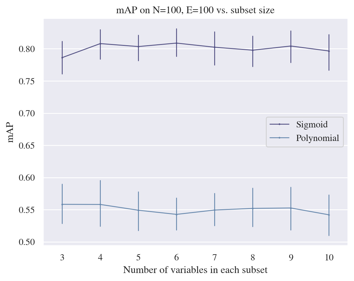
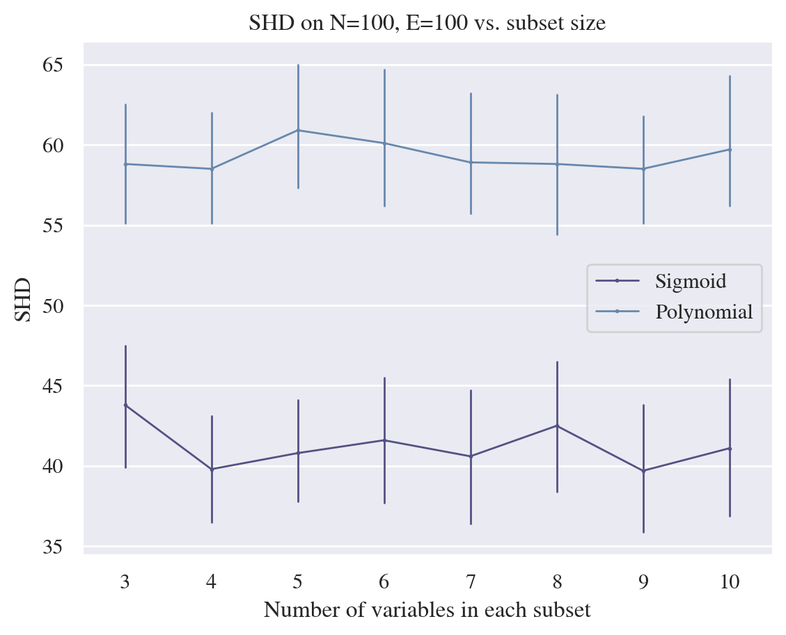
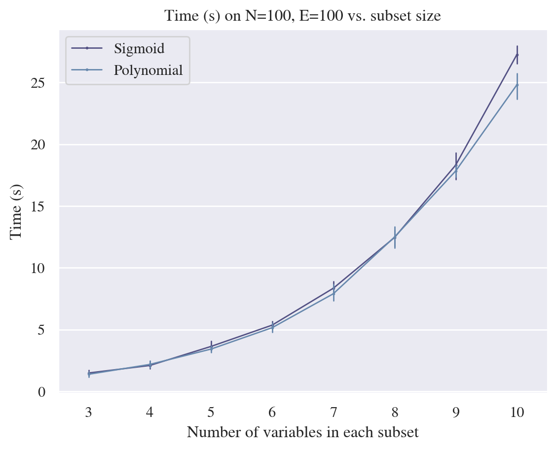
Figure 8: Performance of our model (GIES) as a function of subset size $|S|$ (number of variables sampled). Error bars indicate 95% confidence interval across the 10 datasets of each setting. Our model was trained on $|S|=5$, but it is insensitive to the number of variables sampled per subset at inference. Runtime scales exponentially upwards.

C.2 Choice of global statistic

We selected inverse covariance as our global feature due to its ease of computation and its relationship to partial correlation. For context, we also provide the performance analysis of several alternatives. Tables 6 and 7 compare the results of different graph-level statistics on our synthetic datasets. Discretization thresholds for SHD were obtained by computing the $p^{\text{th}}$ quantile of the computed values, where $p=1-(E/N)$. This is not entirely fair, as no other baseline receives the same calibration, but these ablation studies only seek to compare state-of-the-art causal discovery methods with the “best” possible (oracle) statistical alternatives.

Corr refers to global correlation,

$$\rho_{i,j}=\frac{\mathbb{E}\left(X_{i}X_{j}\right)-\mathbb{E}\left(X_{i}\right)\mathbb{E}\left(X_{j}\right)}{\sqrt{\mathbb{E}\left(X_{i}^{2}\right)-\mathbb{E}\left(X_{i}\right)^{2}}\cdot\sqrt{\mathbb{E}\left(X_{j}^{2}\right)-\mathbb{E}\left(X_{j}\right)^{2}}}.$$ (60)

D-Corr refers to distance correlation, computed between all pairs of variables. Distance correlation captures both linear and non-linear dependencies, and $\textsc{D-Corr}(X_{i},X_{j})=0$ if and only if $X_{i}\perp\!\!\!\perp X_{j}$. Please refer to (Sz’ekely et al., 2007) for the full derivation. Despite its power to capture non-linear dependencies, we opted not to use D-Corr because it is quite slow to compute between all pairs of variables.

InvCov refers to inverse covariance, computed globally,

$$\rho=\mathbb{E}\left((X-\mathbb{E}\left(X\right))(X-\mathbb{E}\left(X\right))^{T}\right)^{-1}.$$ (61)

For graphs $N<100$, inverse covariance was computed directly using NumPy. For graphs $N\geq 100$, inverse covariance was computed using Ledoit-Wolf shrinkage at inference time (Ledoit & Wolf, 2004).

Table 6: Comparison of global statistics (continuous metrics).

$N$	$E$	Model	Linear		NN add.		NN non-add.		Sigmoid		Polynomial
			mAP $\uparrow$	AUC $\uparrow$	mAP $\uparrow$	AUC $\uparrow$	mAP $\uparrow$	AUC $\uparrow$	mAP $\uparrow$	AUC $\uparrow$	mAP $\uparrow$	AUC $\uparrow$
10	10	Corr	$0.45\scriptstyle\pm 0.0$	$0.87\scriptstyle\pm 0.0$	$0.41\scriptstyle\pm 0.0$	$0.86\scriptstyle\pm 0.1$	$0.41\scriptstyle\pm 0.1$	$0.85\scriptstyle\pm 0.0$	$0.46\scriptstyle\pm 0.0$	$0.86\scriptstyle\pm 0.1$	$0.45\scriptstyle\pm 0.0$	$0.85\scriptstyle\pm 0.1$
		D-Corr	$0.42\scriptstyle\pm 0.0$	$0.86\scriptstyle\pm 0.0$	$0.41\scriptstyle\pm 0.1$	$0.87\scriptstyle\pm 0.1$	$0.40\scriptstyle\pm 0.0$	$0.87\scriptstyle\pm 0.0$	$0.43\scriptstyle\pm 0.0$	$0.86\scriptstyle\pm 0.1$	$0.45\scriptstyle\pm 0.0$	$0.89\scriptstyle\pm 0.1$
		InvCov	$0.49\scriptstyle\pm 0.0$	$0.87\scriptstyle\pm 0.0$	$0.45\scriptstyle\pm 0.1$	$0.86\scriptstyle\pm 0.1$	$0.36\scriptstyle\pm 0.1$	$0.81\scriptstyle\pm 0.1$	$0.44\scriptstyle\pm 0.1$	$0.86\scriptstyle\pm 0.1$	$0.45\scriptstyle\pm 0.1$	$0.83\scriptstyle\pm 0.1$
10	40	Corr	$0.47\scriptstyle\pm 0.0$	$0.53\scriptstyle\pm 0.0$	$0.47\scriptstyle\pm 0.0$	$0.52\scriptstyle\pm 0.0$	$0.46\scriptstyle\pm 0.0$	$0.52\scriptstyle\pm 0.0$	$0.48\scriptstyle\pm 0.0$	$0.53\scriptstyle\pm 0.0$	$0.48\scriptstyle\pm 0.0$	$0.54\scriptstyle\pm 0.0$
		D-Corr	$0.46\scriptstyle\pm 0.0$	$0.53\scriptstyle\pm 0.0$	$0.46\scriptstyle\pm 0.0$	$0.51\scriptstyle\pm 0.0$	$0.46\scriptstyle\pm 0.0$	$0.54\scriptstyle\pm 0.0$	$0.48\scriptstyle\pm 0.0$	$0.53\scriptstyle\pm 0.0$	$0.47\scriptstyle\pm 0.0$	$0.54\scriptstyle\pm 0.0$
		InvCov	$0.50\scriptstyle\pm 0.0$	$0.57\scriptstyle\pm 0.0$	$0.48\scriptstyle\pm 0.0$	$0.52\scriptstyle\pm 0.0$	$0.47\scriptstyle\pm 0.0$	$0.53\scriptstyle\pm 0.0$	$0.47\scriptstyle\pm 0.0$	$0.50\scriptstyle\pm 0.0$	$0.48\scriptstyle\pm 0.0$	$0.52\scriptstyle\pm 0.0$
100	100	Corr	$0.42\scriptstyle\pm 0.0$	$0.99\scriptstyle\pm 0.0$	$0.25\scriptstyle\pm 0.0$	$0.94\scriptstyle\pm 0.0$	$0.25\scriptstyle\pm 0.0$	$0.93\scriptstyle\pm 0.0$	$0.42\scriptstyle\pm 0.0$	$0.98\scriptstyle\pm 0.0$	$0.35\scriptstyle\pm 0.0$	$0.91\scriptstyle\pm 0.0$
		D-Corr	$0.41\scriptstyle\pm 0.0$	$0.99\scriptstyle\pm 0.0$	$0.25\scriptstyle\pm 0.0$	$0.96\scriptstyle\pm 0.0$	$0.26\scriptstyle\pm 0.0$	$0.96\scriptstyle\pm 0.0$	$0.41\scriptstyle\pm 0.0$	$0.98\scriptstyle\pm 0.0$	$0.37\scriptstyle\pm 0.0$	$0.94\scriptstyle\pm 0.0$
		InvCov	$0.40\scriptstyle\pm 0.0$	$0.99\scriptstyle\pm 0.0$	$0.22\scriptstyle\pm 0.0$	$0.94\scriptstyle\pm 0.0$	$0.16\scriptstyle\pm 0.0$	$0.87\scriptstyle\pm 0.0$	$0.40\scriptstyle\pm 0.0$	$0.97\scriptstyle\pm 0.0$	$0.36\scriptstyle\pm 0.0$	$0.90\scriptstyle\pm 0.0$
100	400	Corr	$0.19\scriptstyle\pm 0.0$	$0.80\scriptstyle\pm 0.0$	$0.10\scriptstyle\pm 0.0$	$0.63\scriptstyle\pm 0.0$	$0.14\scriptstyle\pm 0.0$	$0.72\scriptstyle\pm 0.0$	$0.27\scriptstyle\pm 0.0$	$0.84\scriptstyle\pm 0.0$	$0.20\scriptstyle\pm 0.0$	$0.72\scriptstyle\pm 0.0$
		D-Corr	$0.19\scriptstyle\pm 0.0$	$0.80\scriptstyle\pm 0.0$	$0.10\scriptstyle\pm 0.0$	$0.63\scriptstyle\pm 0.0$	$0.14\scriptstyle\pm 0.0$	$0.75\scriptstyle\pm 0.0$	$0.26\scriptstyle\pm 0.0$	$0.84\scriptstyle\pm 0.0$	$0.21\scriptstyle\pm 0.0$	$0.74\scriptstyle\pm 0.0$
		InvCov	$0.25\scriptstyle\pm 0.0$	$0.91\scriptstyle\pm 0.0$	$0.09\scriptstyle\pm 0.0$	$0.62\scriptstyle\pm 0.0$	$0.14\scriptstyle\pm 0.0$	$0.77\scriptstyle\pm 0.0$	$0.27\scriptstyle\pm 0.0$	$0.86\scriptstyle\pm 0.0$	$0.20\scriptstyle\pm 0.0$	$0.67\scriptstyle\pm 0.0$

Table 7: Comparison of global statistics (SHD). Discretization thresholds for SHD were obtained by computing the $p^{\text{th}}$ quantile of the computed values, where $p=1-(E/N)$.

$N$	$E$	Model	Linear	NN add.	NN non-add.	Sigmoid	Polynomial
10	10	Corr	$10.6\scriptstyle\pm 2.8$	$10.2\scriptstyle\pm 4.6$	$12.0\scriptstyle\pm 1.9$	$11.1\scriptstyle\pm 4.3$	$9.9\scriptstyle\pm 2.8$
		D-Corr	$10.4\scriptstyle\pm 2.6$	$9.8\scriptstyle\pm 4.7$	$12.2\scriptstyle\pm 2.6$	$10.8\scriptstyle\pm 3.3$	$10.2\scriptstyle\pm 3.2$
		InvCov	$11.0\scriptstyle\pm 2.8$	$11.4\scriptstyle\pm 5.5$	$13.6\scriptstyle\pm 2.9$	$11.4\scriptstyle\pm 4.1$	$10.9\scriptstyle\pm 3.5$
10	40	Corr	$39.2\scriptstyle\pm 2.4$	$38.0\scriptstyle\pm 1.8$	$38.2\scriptstyle\pm 0.7$	$38.8\scriptstyle\pm 3.3$	$38.2\scriptstyle\pm 2.0$
		D-Corr	$38.8\scriptstyle\pm 2.0$	$38.8\scriptstyle\pm 1.5$	$37.0\scriptstyle\pm 0.6$	$38.9\scriptstyle\pm 3.2$	$38.0\scriptstyle\pm 2.0$
		InvCov	$35.8\scriptstyle\pm 2.3$	$39.2\scriptstyle\pm 1.5$	$37.6\scriptstyle\pm 2.7$	$40.7\scriptstyle\pm 2.2$	$38.4\scriptstyle\pm 1.2$
100	100	Corr	$113.0\scriptstyle\pm 4.9$	$132.2\scriptstyle\pm 18.0$	$144.6\scriptstyle\pm 5.2$	$106.5\scriptstyle\pm 11.5$	$110.3\scriptstyle\pm 6.1$
		D-Corr	$113.8\scriptstyle\pm 5.3$	$133.2\scriptstyle\pm 17.9$	$144.2\scriptstyle\pm 6.7$	$108.5\scriptstyle\pm 11.9$	$109.5\scriptstyle\pm 5.7$
		InvCov	$124.4\scriptstyle\pm 8.1$	$130.0\scriptstyle\pm 17.2$	$158.8\scriptstyle\pm 6.2$	$112.3\scriptstyle\pm 14.8$	$106.3\scriptstyle\pm 4.6$
100	400	Corr	$580.4\scriptstyle\pm 24.5$	$666.0\scriptstyle\pm 13.5$	$626.2\scriptstyle\pm 23.4$	$516.5\scriptstyle\pm 18.5$	$562.5\scriptstyle\pm 20.1$
		D-Corr	$578.2\scriptstyle\pm 24.7$	$665.4\scriptstyle\pm 15.4$	$626.6\scriptstyle\pm 21.9$	$522.3\scriptstyle\pm 17.6$	$557.2\scriptstyle\pm 20.4$
		InvCov	$557.0\scriptstyle\pm 11.7$	$667.8\scriptstyle\pm 15.4$	$639.0\scriptstyle\pm 9.7$	$514.7\scriptstyle\pm 23.1$	$539.4\scriptstyle\pm 18.4$

C.3 Results on simulated mRNA data

Table 8: Causal discovery results on simulated mRNA data. Each setting encompasses 5 distinct scale-free graphs. Data were generated via SERGIO (Dibaeinia & Sinha, 2020).

$N$	$E$	Model	mAP $\uparrow$	AUC $\uparrow$	SHD $\downarrow$	EdgeAcc $\uparrow$
10	10	Dcdi-G	$0.48$	$0.73$	$16.1$	$0.70$
		Dcdi-Dsf	$0.63$	$0.84$	$18.5$	$0.81$
		Dcd-Fg	$0.59$	$0.82$	$81.0$	$0.79$
		Sea (Fci)	0.92	0.98	1.9	0.92
10	20	Dcdi-G	$0.32$	$0.57$	$26.2$	$0.59$
		Dcdi-Dsf	$0.44$	$0.64$	$25.7$	$0.64$
		Dcd-Fg	$0.43$	$0.69$	$73.0$	$0.67$
		Sea (Fci)	0.76	0.90	8.8	0.85
20	20	Dcdi-G	$0.48$	$0.86$	$37.3$	$0.90$
		Dcdi-Dsf	$0.45$	$0.92$	$51.9$	0.94
		Dcd-Fg	$0.34$	$0.87$	$361.0$	$0.66$
		Sea (Fci)	0.54	0.94	16.6	$0.83$
20	20	Dcdi-G	$0.31$	$0.65$	$54.7$	$0.72$
		Dcdi-Dsf	$0.40$	$0.71$	$54.6$	$0.74$
		Dcd-Fg	$0.36$	$0.77$	$343.0$	$0.67$
		Sea (Fci)	0.50	0.85	31.4	0.78

We generator mRNA data using the SERGIO simulator (Dibaeinia & Sinha, 2020). We sampled datasets with the Hill coefficient set to $\{0.25,0.5,1,2,4\}$ for training, and 2 for testing (2 was default). We set the decay rate to the default 0.8, and the noise parameter to the default of 1.0. We sampled 400 graphs for each of $N=\{10,20\}$ and $E=\{N,2N\}$.

These data distributions are quite different from typical synthetic datasets, as they simulate steady-state measurements and the data are lower bounded at 0 (gene counts).

C.4 Additional results on synthetic data

Table 9: Comparison between heuristics-based sampler (random and inverse covariance) vs. model confidence-based sampler. Details regarding the samplers can be found in B.6. The suffix -L indicates the greedy confidence-based sampler. Each setting encompasses 5 distinct Erdős-Rényi graphs. The symbol $\dagger$ indicates that Sea was not pretrained on this setting. Bold indicates best of all models considered (including baselines not pictured).

$N$	$E$	Model	Linear			NN add.			NN non-add.			Sigmoid†			Polynomial†
			mAP$\uparrow$	EA$\uparrow$	SHD$\downarrow$	mAP$\uparrow$	EA$\uparrow$	SHD$\downarrow$	mAP$\uparrow$	EA$\uparrow$	SHD$\downarrow$	mAP$\uparrow$	EA$\uparrow$	SHD$\downarrow$	mAP$\uparrow$	EA$\uparrow$	SHD$\downarrow$
10	10	Sea (f)	$0.97$	$0.92$	$1.6$	0.95	0.92	$2.4$	0.92	$0.94$	$2.8$	$0.83$	$0.76$	$3.7$	$0.69$	$0.71$	$6.7$
		Sea (g)	0.99	0.94	$1.2$	$0.94$	$0.88$	$2.6$	$0.91$	$0.93$	$3.2$	$0.85$	$0.84$	$4.0$	$0.70$	$0.79$	5.8
		Sea (f)-l	$0.97$	$0.93$	1.0	$0.95$	$0.87$	$2.4$	0.92	0.98	$3.4$	$0.84$	$0.77$	$3.9$	0.70	$0.79$	5.8
		Sea (g)-l	$0.98$	$0.93$	$1.4$	$0.94$	$0.91$	$2.8$	$0.91$	$0.94$	$4.0$	0.88	0.84	3.6	$0.70$	0.80	5.8
10	40	Sea (f)	$0.90$	$0.87$	$14.4$	$0.91$	$0.94$	$11.2$	$0.87$	$0.86$	$16.0$	0.81	$0.85$	$22.7$	$0.81$	$0.92$	$33.4$
		Sea (g)	0.94	0.91	12.8	$0.91$	0.95	10.4	0.89	0.89	$17.2$	$0.81$	0.87	$24.5$	$0.89$	$0.93$	$29.5$
		Sea (f)-l	$0.91$	$0.90$	$15.6$	0.91	$0.92$	$15.8$	$0.88$	$0.86$	$14.2$	$0.81$	$0.84$	$23.2$	$0.82$	$0.93$	$33.8$
		Sea (g)-l	$0.93$	$0.91$	$13.4$	$0.91$	$0.93$	10.4	$0.88$	$0.85$	$16.2$	$0.79$	$0.83$	$25.5$	0.90	0.94	$28.3$
20	20	Sea (f)	$0.97$	$0.92$	$3.2$	$0.94$	$0.97$	$3.2$	$0.84$	$0.93$	$7.2$	$0.84$	$0.85$	$7.6$	0.71	0.80	$10.2$
		Sea (g)	$0.97$	$0.89$	$3.0$	0.94	$0.95$	$3.4$	$0.83$	$0.94$	$7.8$	$0.84$	$0.83$	$8.1$	$0.69$	$0.78$	$10.1$
		Sea (f)-l	$0.97$	0.92	$2.8$	$0.93$	$0.95$	$3.8$	0.85	$0.94$	$6.8$	0.85	$0.85$	7.5	$0.67$	$0.78$	9.9
		Sea (g)-l	0.97	$0.90$	2.6	0.94	0.98	$3.4$	$0.83$	0.97	$7.0$	$0.84$	$0.84$	$7.9$	$0.67$	$0.79$	$10.6$
20	80	Sea (f)	$0.86$	0.93	$29.6$	$0.55$	$0.90$	$73.6$	$0.72$	0.93	$51.8$	0.77	$0.85$	$42.8$	$0.61$	$0.89$	$61.8$
		Sea (g)	0.89	$0.92$	26.8	0.58	$0.88$	$71.4$	$0.73$	$0.92$	$50.6$	$0.76$	$0.84$	$45.0$	0.65	0.89	$60.1$
		Sea (f)-l	$0.86$	$0.92$	$32.0$	$0.55$	0.90	$74.0$	$0.74$	$0.93$	$49.2$	$0.76$	0.87	41.8	$0.59$	$0.88$	$62.3$
		Sea (g)-l	0.89	$0.92$	$28.4$	$0.58$	$0.89$	$71.6$	$0.75$	$0.92$	$49.4$	$0.75$	$0.85$	$45.7$	0.65	$0.88$	$60.6$

Table 10: Scaling to synthetic graphs, larger than those seen in training. Each setting encompasses 5 distinct Erdős-Rényi graphs. For all analysis in this table, we took $T=500$ subsets of nodes, with $b=500$ examples per batch. Here, the mean AUC values are artificially high due to the high negative rates, as actual edges scale linearly as $N$, while the number of possible edges scales quadratically.

$N$	Model	Linear, $E=N$					Linear, $E=4N$
		mAP $\uparrow$	AUC $\uparrow$	SHD $\downarrow$	EdgeAcc $\uparrow$		mAP $\uparrow$	AUC $\uparrow$	SHD $\downarrow$	EdgeAcc $\uparrow$
100	InvCov	$0.43\scriptstyle\pm 0.0$	$0.99\scriptstyle\pm 0.0$	$116.8\scriptstyle\pm 7$	—		$0.30\scriptstyle\pm 0.0$	$0.93\scriptstyle\pm 0.0$	$511.8\scriptstyle\pm 11$	—
	Corr	$0.42\scriptstyle\pm 0.0$	$0.99\scriptstyle\pm 0.0$	$113.0\scriptstyle\pm 5$	—		$0.19\scriptstyle\pm 0.0$	$0.80\scriptstyle\pm 0.0$	$579.4\scriptstyle\pm 25$	—
	Sea (Fci)	$0.97\scriptstyle\pm 0.0$	$1.00\scriptstyle\pm 0.0$	$11.6\scriptstyle\pm 4$	$0.93\scriptstyle\pm 0.0$		$0.88\scriptstyle\pm 0.0$	$0.98\scriptstyle\pm 0.0$	$129.0\scriptstyle\pm 10$	$0.94\scriptstyle\pm 0.0$
	Sea (Gies)	$0.97\scriptstyle\pm 0.0$	$1.00\scriptstyle\pm 0.0$	$12.8\scriptstyle\pm 5$	$0.91\scriptstyle\pm 0.0$		$0.91\scriptstyle\pm 0.0$	$0.99\scriptstyle\pm 0.0$	$104.6\scriptstyle\pm 6$	$0.95\scriptstyle\pm 0.0$
200	InvCov	$0.45\scriptstyle\pm 0.0$	$1.00\scriptstyle\pm 0.0$	$218.4\scriptstyle\pm 11$	—		$0.33\scriptstyle\pm 0.0$	$0.96\scriptstyle\pm 0.0$	$999.6\scriptstyle\pm 23$	—
	Corr	$0.42\scriptstyle\pm 0.0$	$0.99\scriptstyle\pm 0.0$	$223.0\scriptstyle\pm 8$	—		$0.18\scriptstyle\pm 0.0$	$0.86\scriptstyle\pm 0.0$	$1183.5\scriptstyle\pm 25$	—
	Sea (Fci)	$0.91\scriptstyle\pm 0.0$	$1.00\scriptstyle\pm 0.0$	$49.9\scriptstyle\pm 5$	$0.87\scriptstyle\pm 0.0$		$0.82\scriptstyle\pm 0.0$	$0.97\scriptstyle\pm 0.0$	$327.4\scriptstyle\pm 52$	$0.92\scriptstyle\pm 0.0$
	Sea (Gies)	$0.95\scriptstyle\pm 0.0$	$1.00\scriptstyle\pm 0.0$	$35.4\scriptstyle\pm 6$	$0.91\scriptstyle\pm 0.0$		$0.86\scriptstyle\pm 0.0$	$0.98\scriptstyle\pm 0.0$	$271.9\scriptstyle\pm 50$	$0.92\scriptstyle\pm 0.0$
300	InvCov	$0.46\scriptstyle\pm 0.0$	$1.00\scriptstyle\pm 0.0$	$308.3\scriptstyle\pm 20$	—		$0.35\scriptstyle\pm 0.0$	$0.98\scriptstyle\pm 0.0$	$1444.7\scriptstyle\pm 56$	—
	Corr	$0.42\scriptstyle\pm 0.0$	$1.00\scriptstyle\pm 0.0$	$326.2\scriptstyle\pm 21$	—		$0.20\scriptstyle\pm 0.0$	$0.89\scriptstyle\pm 0.0$	$1710.4\scriptstyle\pm 82$	—
	Sea (Fci)	$0.80\scriptstyle\pm 0.0$	$1.00\scriptstyle\pm 0.0$	$121.1\scriptstyle\pm 14$	$0.78\scriptstyle\pm 0.0$		$0.70\scriptstyle\pm 0.0$	$0.95\scriptstyle\pm 0.0$	$693.1\scriptstyle\pm 67$	$0.86\scriptstyle\pm 0.0$
	Sea (Gies)	$0.88\scriptstyle\pm 0.0$	$1.00\scriptstyle\pm 0.0$	$88.9\scriptstyle\pm 11$	$0.84\scriptstyle\pm 0.0$		$0.78\scriptstyle\pm 0.0$	$0.96\scriptstyle\pm 0.0$	$556.1\scriptstyle\pm 71$	$0.87\scriptstyle\pm 0.0$
400	InvCov	$0.47\scriptstyle\pm 0.0$	$1.00\scriptstyle\pm 0.0$	$417.7\scriptstyle\pm 7$	—		$0.36\scriptstyle\pm 0.0$	$0.98\scriptstyle\pm 0.0$	$1882.7\scriptstyle\pm 28$	—
	Corr	$0.42\scriptstyle\pm 0.0$	$1.00\scriptstyle\pm 0.0$	$445.4\scriptstyle\pm 14$	—		$0.20\scriptstyle\pm 0.0$	$0.91\scriptstyle\pm 0.0$	$2269.3\scriptstyle\pm 52$	—
	Sea (Fci)	$0.49\scriptstyle\pm 0.2$	$0.93\scriptstyle\pm 0.1$	$313.9\scriptstyle\pm 107$	$0.61\scriptstyle\pm 0.1$		$0.56\scriptstyle\pm 0.1$	$0.90\scriptstyle\pm 0.1$	$1103.1\scriptstyle\pm 190$	$0.75\scriptstyle\pm 0.1$
	Sea (Gies)	$0.70\scriptstyle\pm 0.1$	$0.99\scriptstyle\pm 0.0$	$225.9\scriptstyle\pm 57$	$0.71\scriptstyle\pm 0.1$		$0.70\scriptstyle\pm 0.0$	$0.94\scriptstyle\pm 0.0$	$871.6\scriptstyle\pm 44$	$0.80\scriptstyle\pm 0.0$
500	InvCov	$0.47\scriptstyle\pm 0.0$	$1.00\scriptstyle\pm 0.0$	$504.5\scriptstyle\pm 19$	—		$0.38\scriptstyle\pm 0.0$	$0.99\scriptstyle\pm 0.0$	$2299.8\scriptstyle\pm 34$	—
	Corr	$0.42\scriptstyle\pm 0.0$	$1.00\scriptstyle\pm 0.0$	$543.3\scriptstyle\pm 18$	—		$0.21\scriptstyle\pm 0.0$	$0.93\scriptstyle\pm 0.0$	$2789.5\scriptstyle\pm 78$	—
	Sea (Fci)	$0.27\scriptstyle\pm 0.1$	$0.90\scriptstyle\pm 0.1$	$757.6\scriptstyle\pm 297$	$0.51\scriptstyle\pm 0.0$		$0.29\scriptstyle\pm 0.1$	$0.86\scriptstyle\pm 0.1$	$1823.6\scriptstyle\pm 273$	$0.56\scriptstyle\pm 0.1$
	Sea (Gies)	$0.41\scriptstyle\pm 0.2$	$0.98\scriptstyle\pm 0.0$	$485.3\scriptstyle\pm 170$	$0.57\scriptstyle\pm 0.1$		$0.48\scriptstyle\pm 0.1$	$0.92\scriptstyle\pm 0.0$	$1653.5\scriptstyle\pm 505$	$0.67\scriptstyle\pm 0.0$

Table 11: Generalization limits of our current implementations. Each setting represents 5 distinct graphs. Our models were not pretrained on multiplicative noise, so they do not generalize reliably to these cases. While much slower, Dcdi variants learn the data distribution from scratch each time, so they seem to perform well in some of these cases. We anticipate that training on multiplicative data would alleviate this generalization gap, but we did not have time to test this empirically.

$N$	$E$	Model	Sigmoid mix†			Polynomial mix†			Sigmoid mix (SF)†			Polynomial mix (SF)†
			mAP $\uparrow$	EA $\uparrow$	SHD $\downarrow$	mAP $\uparrow$	EA $\uparrow$	SHD $\downarrow$	mAP $\uparrow$	EA $\uparrow$	SHD $\downarrow$	mAP $\uparrow$	EA $\uparrow$	SHD $\downarrow$
10	10	Dcdi-G	$0.84$	$0.81$	$0.9$	$0.11$	$0.00$	$10.2$	$0.67$	$0.92$	$15.2$	$0.12$	$0.00$	$10.6$
		Dcdi-Dsf	0.96	0.91	0.3	0.39	$0.32$	7.3	$0.81$	0.98	$13.6$	0.39	$0.36$	9.8
		Dcd-Fg	$0.52$	$0.61$	$18.0$	$0.11$	$0.00$	$10.2$	$0.57$	$0.66$	$15.5$	$0.12$	$0.00$	$10.6$
		DiffAn	$0.14$	$0.31$	$19.9$	$0.11$	$0.09$	$14.0$	$0.10$	$0.22$	$17.8$	$0.11$	$0.14$	$17.2$
		Deci	$0.17$	$0.43$	$19.1$	$0.11$	$0.07$	$14.1$	$0.20$	$0.53$	$15.0$	$0.12$	$0.06$	$13.6$
		InvCov	$0.34$	$0.51$	$12.1$	$0.18$	$0.51$	$16.4$	$0.31$	$0.56$	$11.4$	$0.16$	$0.50$	$16.1$
		Fci-Avg	$0.56$	$0.54$	$9.1$	$0.11$	$0.00$	$10.2$	$0.53$	$0.52$	$8.1$	$0.12$	$0.01$	$10.6$
		Gies-Avg	$0.91$	$0.88$	$3.1$	$0.22$	$0.38$	$10.2$	0.93	$0.88$	2.3	$0.22$	$0.37$	$10.6$
		Sea (Fci)	$0.58$	$0.51$	$5.7$	$0.25$	0.53	$10.2$	$0.67$	$0.56$	$4.5$	$0.20$	0.46	$10.6$
		Sea (Gies)	$0.41$	$0.39$	$8.1$	$0.18$	$0.51$	$10.2$	$0.48$	$0.48$	$5.4$	$0.21$	0.46	$10.6$
10	40	Dcdi-G	$0.58$	$0.35$	$25.0$	$0.44$	$0.00$	$39.8$	$0.76$	$0.83$	$22.0$	$0.31$	$0.00$	$28.2$
		Dcdi-Dsf	0.79	$0.46$	12.2	$0.48$	$0.09$	$35.6$	0.92	0.88	15.8	$0.35$	$0.07$	26.4
		Dcd-Fg	$0.60$	$0.40$	$26.8$	$0.44$	$0.00$	$39.8$	$0.52$	$0.46$	$22.1$	$0.31$	$0.00$	$28.2$
		DiffAn	$0.38$	$0.32$	$31.8$	$0.40$	$0.32$	30.0	$0.26$	$0.30$	$35.0$	$0.28$	$0.29$	$29.3$
		Deci	$0.46$	$0.39$	$27.5$	$0.43$	$0.03$	$39.5$	$0.35$	$0.51$	$24.9$	$0.30$	$0.05$	$30.1$
		InvCov	$0.48$	$0.51$	$38.7$	$0.48$	$0.54$	$40.3$	$0.40$	$0.51$	$32.5$	$0.34$	$0.48$	$38.2$
		Fci-Avg	$0.44$	$0.18$	$39.7$	$0.44$	$0.01$	$39.8$	$0.43$	$0.30$	$25.2$	$0.32$	$0.01$	$28.2$
		Gies-Avg	$0.43$	$0.37$	$38.2$	$0.50$	$0.48$	$39.8$	$0.48$	$0.45$	$22.8$	$0.36$	$0.39$	$28.2$
		Sea (Fci)	$0.56$	$0.58$	$28.6$	0.81	$0.85$	$39.7$	$0.62$	$0.67$	$17.3$	$0.58$	0.85	$28.2$
		Sea (Gies)	$0.58$	0.65	$30.2$	$0.80$	0.86	$39.5$	$0.64$	$0.69$	$16.7$	0.60	$0.81$	$28.2$
20	20	Dcdi-G	$0.57$	$0.72$	$6.2$	$0.06$	$0.01$	$21.7$	$0.47$	0.98	$45.4$	$0.06$	$0.01$	20.7
		Dcdi-Dsf	0.91	0.94	1.1	0.21	$0.46$	$34.6$	$0.56$	$0.97$	$40.6$	0.29	0.80	$83.0$
		Dcd-Fg	$0.50$	$0.68$	$62.1$	$0.06$	$0.00$	$24.3$	$0.63$	$0.81$	$256.6$	$0.06$	$0.11$	$186.4$
		DiffAn	$0.08$	$0.26$	$47.5$	$0.06$	$0.15$	$51.5$	$0.08$	$0.30$	$42.6$	$0.06$	$0.22$	$53.7$
		Deci	$0.17$	$0.58$	$38.0$	$0.06$	$0.05$	$36.0$	$0.18$	$0.60$	$32.9$	$0.06$	$0.03$	$38.9$
		InvCov	$0.31$	$0.59$	$22.3$	$0.09$	$0.52$	$35.9$	$0.24$	$0.44$	$24.5$	$0.07$	$0.50$	$35.4$
		Fci-Avg	$0.64$	$0.69$	$17.4$	$0.06$	$0.01$	21.3	$0.58$	$0.66$	$15.3$	$0.06$	$0.00$	$21.0$
		Gies-Avg	$0.82$	$0.75$	$8.5$	$0.15$	$0.44$	21.3	0.83	$0.78$	7.8	$0.12$	$0.42$	$21.0$
		Sea (Fci)	$0.61$	$0.60$	$8.5$	$0.12$	0.55	21.3	$0.63$	$0.56$	$9.0$	$0.11$	$0.55$	$21.1$
		Sea (Gies)	$0.41$	$0.48$	$13.0$	$0.11$	$0.55$	$21.6$	$0.50$	$0.49$	$12.3$	$0.11$	$0.52$	$21.3$
20	80	Dcdi-G	$0.60$	$0.59$	$32.3$	$0.21$	$0.05$	$86.4$	$0.54$	$0.84$	$78.6$	$0.18$	$0.14$	$74.8$
		Dcdi-Dsf	0.89	0.81	8.4	$0.24$	$0.25$	$102.3$	0.65	0.89	$60.1$	$0.27$	$0.60$	$201.6$
		Dcd-Fg	$0.46$	$0.72$	$222.2$	$0.21$	$0.00$	$81.8$	$0.52$	$0.76$	$202.2$	$0.18$	$0.15$	$225.9$
		DiffAn	$0.18$	$0.30$	$151.1$	$0.19$	$0.31$	$130.8$	$0.15$	$0.30$	$137.0$	$0.16$	$0.31$	$127.9$
		Deci	$0.31$	$0.43$	$70.5$	$0.20$	$0.03$	$89.0$	$0.25$	$0.41$	$66.5$	$0.17$	$0.02$	$79.0$
		InvCov	$0.30$	$0.51$	$98.1$	$0.22$	$0.51$	$115.4$	$0.27$	$0.53$	$89.1$	$0.19$	$0.49$	$108.1$
		Fci-Avg	$0.37$	$0.30$	$76.0$	$0.21$	$0.01$	$79.3$	$0.38$	$0.34$	$59.6$	$0.18$	$0.01$	66.5
		Gies-Avg	$0.54$	$0.64$	$68.4$	$0.23$	$0.37$	$79.3$	$0.55$	$0.65$	$50.7$	$0.19$	$0.36$	66.5
		Sea (Fci)	$0.61$	$0.64$	$52.6$	$0.41$	0.87	$79.3$	$0.62$	$0.70$	36.7	$0.34$	$0.82$	$66.7$
		Sea (Gies)	$0.53$	$0.64$	$58.1$	0.43	$0.86$	79.0	$0.59$	$0.74$	$41.4$	0.35	0.82	$66.8$

Table 12: Causal discovery results on synthetic datasets with 100 nodes, continuous metrics. Each setting encompasses 5 distinct Erdős-Rényi graphs. The symbol $\dagger$ indicates that the model was not trained on this setting. All standard deviations were within 0.1.

$N$	$E$	Model	Linear		NN add.		NN non-add.		Sigmoid†		Polynomial†
			mAP $\uparrow$	AUC $\uparrow$	mAP $\uparrow$	AUC $\uparrow$	mAP $\uparrow$	AUC $\uparrow$	mAP $\uparrow$	AUC $\uparrow$	mAP $\uparrow$	AUC $\uparrow$
100	100	Dcd-Fg	$0.11$	$0.75$	$0.12$	$0.71$	$0.18$	$0.73$	$0.20$	$0.72$	$0.06$	$0.60$
		InvCov	$0.40$	$0.99$	$0.22$	$0.94$	$0.16$	$0.87$	$0.40$	$0.97$	$0.36$	$0.90$
		Sea (Fci)	$0.96$	$1.00$	$0.83$	$0.97$	$0.75$	$0.97$	$0.79$	$0.97$	$0.56$	$0.88$
		Sea (Gies)	$0.97$	$1.00$	$0.82$	$0.98$	$0.74$	$0.96$	$0.80$	$0.97$	$0.54$	$0.85$
100	400	Dcd-Fg	$0.05$	$0.59$	$0.07$	$0.64$	$0.10$	$0.72$	$0.13$	$0.72$	$0.12$	$0.64$
		InvCov	$0.25$	$0.91$	$0.09$	$0.62$	$0.14$	$0.77$	$0.27$	$0.86$	$0.20$	$0.67$
		Sea (Fci)	$0.90$	$0.99$	$0.28$	$0.82$	$0.60$	$0.92$	$0.69$	$0.92$	$0.38$	$0.80$
		Sea (Gies)	$0.91$	$0.99$	$0.27$	$0.82$	$0.61$	$0.92$	$0.69$	$0.91$	$0.38$	$0.78$

Table 13: Causal discovery results on synthetic datasets with 100 nodes, discrete metrics. Each setting encompasses 5 distinct Erdős-Rényi graphs. The symbol $\dagger$ indicates that the model was not trained on this setting.

$N$	$E$	Model	Linear		NN add.		NN non-add.		Sigmoid†		Polynomial†
			EdgeAcc $\uparrow$	SHD $\downarrow$	EdgeAcc $\uparrow$	SHD $\downarrow$	EdgeAcc $\uparrow$	SHD $\downarrow$	EdgeAcc $\uparrow$	SHD $\downarrow$	EdgeAcc $\uparrow$	SHD $\downarrow$
100	100	Dcd-Fg	$0.63$	$3075.8$	$0.58$	$2965.0$	$0.60$	$2544.4$	$0.59$	$3808.0$	$0.34$	$1927.9$
		InvCov	—	$124.4$	—	$130.0$	—	$158.8$	—	$112.3$	—	$106.3$
		Sea (Fci)	$0.91$	$13.4$	$0.90$	$34.4$	$0.91$	$47.2$	$0.78$	$40.3$	$0.69$	$59.2$
		Sea (Gies)	$0.91$	$13.6$	$0.93$	$32.8$	$0.91$	$45.8$	$0.78$	$38.6$	$0.68$	$60.3$
100	400	Dcd-Fg	$0.46$	$3068.2$	$0.60$	$3428.8$	$0.70$	$3510.8$	$0.67$	$3601.8$	$0.53$	$3316.7$
		InvCov	—	$557.0$	—	$667.8$	—	$639.0$	—	$514.7$	—	$539.4$
		Sea (Fci)	$0.93$	$122.0$	$0.90$	$361.2$	$0.91$	$273.2$	$0.87$	$226.9$	$0.82$	$327.0$
		Sea (Gies)	$0.94$	$116.6$	$0.91$	$364.4$	$0.92$	$266.8$	$0.87$	$218.3$	$0.84$	$328.0$

Table 14: Causal discovery results on synthetic scale-free datasets, continuous metrics. Each setting encompasses 5 distinct scale-free graphs. The symbol $\dagger$ indicates that Sea was not pretrained on this setting. Details regarding baselines can be found in B.2.

$N$	$E$	Model	Linear		NN add.		NN non-add.		Sigmoid†		Polynomial†
			mAP $\uparrow$	AUC $\uparrow$	mAP $\uparrow$	AUC $\uparrow$	mAP $\uparrow$	AUC $\uparrow$	mAP $\uparrow$	AUC $\uparrow$	mAP $\uparrow$	AUC $\uparrow$
10	10	Dcdi-G	$0.54\scriptstyle\pm 0.2$	$0.90\scriptstyle\pm 0.0$	$0.59\scriptstyle\pm 0.1$	$0.88\scriptstyle\pm 0.1$	$0.69\scriptstyle\pm 0.1$	$0.89\scriptstyle\pm 0.0$	$0.48\scriptstyle\pm 0.2$	$0.77\scriptstyle\pm 0.1$	$0.50\scriptstyle\pm 0.2$	$0.73\scriptstyle\pm 0.1$
		Dcdi-Dsf	$0.70\scriptstyle\pm 0.2$	$0.92\scriptstyle\pm 0.1$	$0.71\scriptstyle\pm 0.2$	$0.88\scriptstyle\pm 0.1$	$0.36\scriptstyle\pm 0.1$	$0.83\scriptstyle\pm 0.1$	$0.46\scriptstyle\pm 0.2$	$0.75\scriptstyle\pm 0.1$	$0.49\scriptstyle\pm 0.1$	$0.76\scriptstyle\pm 0.1$
		Dcd-Fg	$0.56\scriptstyle\pm 0.1$	$0.76\scriptstyle\pm 0.1$	$0.47\scriptstyle\pm 0.1$	$0.72\scriptstyle\pm 0.1$	$0.50\scriptstyle\pm 0.2$	$0.73\scriptstyle\pm 0.1$	$0.44\scriptstyle\pm 0.2$	$0.68\scriptstyle\pm 0.1$	$0.57\scriptstyle\pm 0.2$	$0.75\scriptstyle\pm 0.1$
		DiffAn	$0.25\scriptstyle\pm 0.1$	$0.73\scriptstyle\pm 0.1$	$0.15\scriptstyle\pm 0.0$	$0.66\scriptstyle\pm 0.0$	$0.16\scriptstyle\pm 0.1$	$0.62\scriptstyle\pm 0.1$	$0.31\scriptstyle\pm 0.1$	$0.75\scriptstyle\pm 0.1$	$0.24\scriptstyle\pm 0.3$	$0.63\scriptstyle\pm 0.1$
		Deci	$0.17\scriptstyle\pm 0.1$	$0.65\scriptstyle\pm 0.1$	$0.17\scriptstyle\pm 0.0$	$0.67\scriptstyle\pm 0.0$	$0.20\scriptstyle\pm 0.0$	$0.72\scriptstyle\pm 0.1$	$0.27\scriptstyle\pm 0.1$	$0.73\scriptstyle\pm 0.1$	$0.49\scriptstyle\pm 0.3$	$0.82\scriptstyle\pm 0.1$
		InvCov	$0.38\scriptstyle\pm 0.1$	$0.57\scriptstyle\pm 0.2$	$0.26\scriptstyle\pm 0.1$	$0.50\scriptstyle\pm 0.1$	$0.29\scriptstyle\pm 0.1$	$0.52\scriptstyle\pm 0.1$	$0.27\scriptstyle\pm 0.1$	$0.46\scriptstyle\pm 0.1$	$0.08\scriptstyle\pm 0.0$	$0.13\scriptstyle\pm 0.1$
		Fci-Avg	$0.56\scriptstyle\pm 0.2$	$0.80\scriptstyle\pm 0.1$	$0.51\scriptstyle\pm 0.2$	$0.80\scriptstyle\pm 0.2$	$0.43\scriptstyle\pm 0.2$	$0.74\scriptstyle\pm 0.1$	$0.60\scriptstyle\pm 0.2$	$0.82\scriptstyle\pm 0.1$	$0.34\scriptstyle\pm 0.1$	$0.68\scriptstyle\pm 0.1$
		Gies-Avg	$0.87\scriptstyle\pm 0.1$	$0.98\scriptstyle\pm 0.0$	$0.61\scriptstyle\pm 0.1$	$0.94\scriptstyle\pm 0.0$	$0.69\scriptstyle\pm 0.1$	$0.94\scriptstyle\pm 0.0$	$0.75\scriptstyle\pm 0.1$	$0.96\scriptstyle\pm 0.0$	$0.71\scriptstyle\pm 0.1$	$0.91\scriptstyle\pm 0.1$
		Sea (Fci)	$0.94\scriptstyle\pm 0.1$	$\textbf{0.99}\scriptstyle\pm 0.0$	$0.93\scriptstyle\pm 0.0$	$\textbf{0.98}\scriptstyle\pm 0.0$	$\textbf{0.93}\scriptstyle\pm 0.1$	$0.98\scriptstyle\pm 0.0$	$0.81\scriptstyle\pm 0.1$	$0.97\scriptstyle\pm 0.0$	$\textbf{0.76}\scriptstyle\pm 0.1$	$\textbf{0.91}\scriptstyle\pm 0.1$
		Sea (Gies)	$\textbf{0.95}\scriptstyle\pm 0.0$	$\textbf{0.99}\scriptstyle\pm 0.0$	$\textbf{0.94}\scriptstyle\pm 0.0$	$\textbf{0.98}\scriptstyle\pm 0.0$	$0.92\scriptstyle\pm 0.0$	$\textbf{0.98}\scriptstyle\pm 0.0$	$\textbf{0.85}\scriptstyle\pm 0.1$	$\textbf{0.98}\scriptstyle\pm 0.0$	$0.74\scriptstyle\pm 0.1$	$0.90\scriptstyle\pm 0.1$
10	40	Dcdi-G	$0.70\scriptstyle\pm 0.0$	$0.85\scriptstyle\pm 0.0$	$0.74\scriptstyle\pm 0.1$	$0.85\scriptstyle\pm 0.1$	$\textbf{0.88}\scriptstyle\pm 0.0$	$\textbf{0.91}\scriptstyle\pm 0.0$	$0.56\scriptstyle\pm 0.1$	$0.66\scriptstyle\pm 0.1$	$0.53\scriptstyle\pm 0.1$	$0.64\scriptstyle\pm 0.1$
		Dcdi-Dsf	$0.74\scriptstyle\pm 0.1$	$0.87\scriptstyle\pm 0.1$	$0.73\scriptstyle\pm 0.1$	$0.84\scriptstyle\pm 0.0$	$0.71\scriptstyle\pm 0.1$	$0.90\scriptstyle\pm 0.0$	$0.56\scriptstyle\pm 0.1$	$0.69\scriptstyle\pm 0.1$	$0.51\scriptstyle\pm 0.0$	$0.63\scriptstyle\pm 0.1$
		Dcd-Fg	$0.37\scriptstyle\pm 0.0$	$0.58\scriptstyle\pm 0.0$	$0.45\scriptstyle\pm 0.1$	$0.61\scriptstyle\pm 0.1$	$0.45\scriptstyle\pm 0.2$	$0.58\scriptstyle\pm 0.1$	$0.49\scriptstyle\pm 0.1$	$0.63\scriptstyle\pm 0.1$	$0.63\scriptstyle\pm 0.1$	$0.73\scriptstyle\pm 0.1$
		DiffAn	$0.29\scriptstyle\pm 0.1$	$0.50\scriptstyle\pm 0.1$	$0.25\scriptstyle\pm 0.0$	$0.38\scriptstyle\pm 0.1$	$0.28\scriptstyle\pm 0.0$	$0.46\scriptstyle\pm 0.1$	$0.31\scriptstyle\pm 0.1$	$0.53\scriptstyle\pm 0.1$	$0.27\scriptstyle\pm 0.0$	$0.44\scriptstyle\pm 0.1$
		Deci	$0.30\scriptstyle\pm 0.0$	$0.51\scriptstyle\pm 0.1$	$0.41\scriptstyle\pm 0.0$	$0.65\scriptstyle\pm 0.1$	$0.33\scriptstyle\pm 0.0$	$0.51\scriptstyle\pm 0.0$	$0.38\scriptstyle\pm 0.1$	$0.60\scriptstyle\pm 0.1$	$0.59\scriptstyle\pm 0.1$	$0.77\scriptstyle\pm 0.1$
		InvCov	$0.36\scriptstyle\pm 0.0$	$0.48\scriptstyle\pm 0.1$	$0.34\scriptstyle\pm 0.0$	$0.49\scriptstyle\pm 0.1$	$0.37\scriptstyle\pm 0.0$	$0.48\scriptstyle\pm 0.0$	$0.39\scriptstyle\pm 0.0$	$0.54\scriptstyle\pm 0.1$	$0.26\scriptstyle\pm 0.0$	$0.34\scriptstyle\pm 0.0$
		Fci-Avg	$0.47\scriptstyle\pm 0.1$	$0.64\scriptstyle\pm 0.0$	$0.41\scriptstyle\pm 0.1$	$0.60\scriptstyle\pm 0.0$	$0.40\scriptstyle\pm 0.0$	$0.58\scriptstyle\pm 0.0$	$0.48\scriptstyle\pm 0.1$	$0.64\scriptstyle\pm 0.1$	$0.41\scriptstyle\pm 0.1$	$0.59\scriptstyle\pm 0.1$
		Gies-Avg	$0.43\scriptstyle\pm 0.1$	$0.68\scriptstyle\pm 0.1$	$0.43\scriptstyle\pm 0.1$	$0.63\scriptstyle\pm 0.1$	$0.44\scriptstyle\pm 0.1$	$0.61\scriptstyle\pm 0.1$	$0.49\scriptstyle\pm 0.1$	$0.69\scriptstyle\pm 0.1$	$0.59\scriptstyle\pm 0.1$	$0.71\scriptstyle\pm 0.1$
		Sea (Fci)	$\textbf{0.93}\scriptstyle\pm 0.0$	$0.96\scriptstyle\pm 0.0$	$0.84\scriptstyle\pm 0.0$	$0.92\scriptstyle\pm 0.0$	$0.81\scriptstyle\pm 0.0$	$0.90\scriptstyle\pm 0.0$	$\textbf{0.81}\scriptstyle\pm 0.0$	$\textbf{0.89}\scriptstyle\pm 0.0$	$0.73\scriptstyle\pm 0.1$	$0.84\scriptstyle\pm 0.0$
		Sea (Gies)	$0.92\scriptstyle\pm 0.0$	$\textbf{0.96}\scriptstyle\pm 0.0$	$\textbf{0.84}\scriptstyle\pm 0.1$	$\textbf{0.93}\scriptstyle\pm 0.0$	$0.83\scriptstyle\pm 0.0$	$0.90\scriptstyle\pm 0.0$	$0.79\scriptstyle\pm 0.0$	$0.88\scriptstyle\pm 0.0$	$\textbf{0.78}\scriptstyle\pm 0.1$	$\textbf{0.87}\scriptstyle\pm 0.0$
20	20	Dcdi-G	$0.41\scriptstyle\pm 0.0$	$0.95\scriptstyle\pm 0.0$	$0.50\scriptstyle\pm 0.1$	$0.94\scriptstyle\pm 0.0$	$0.69\scriptstyle\pm 0.1$	$0.96\scriptstyle\pm 0.0$	$0.37\scriptstyle\pm 0.0$	$0.83\scriptstyle\pm 0.1$	$0.37\scriptstyle\pm 0.1$	$0.77\scriptstyle\pm 0.1$
		Dcdi-Dsf	$0.48\scriptstyle\pm 0.0$	$0.95\scriptstyle\pm 0.0$	$0.55\scriptstyle\pm 0.1$	$0.93\scriptstyle\pm 0.0$	$0.33\scriptstyle\pm 0.1$	$0.90\scriptstyle\pm 0.0$	$0.37\scriptstyle\pm 0.1$	$0.79\scriptstyle\pm 0.1$	$0.35\scriptstyle\pm 0.1$	$0.82\scriptstyle\pm 0.1$
		Dcd-Fg	$0.51\scriptstyle\pm 0.1$	$0.87\scriptstyle\pm 0.1$	$0.39\scriptstyle\pm 0.1$	$0.83\scriptstyle\pm 0.1$	$0.48\scriptstyle\pm 0.1$	$0.84\scriptstyle\pm 0.0$	$0.56\scriptstyle\pm 0.1$	$0.84\scriptstyle\pm 0.1$	$0.50\scriptstyle\pm 0.1$	$0.84\scriptstyle\pm 0.1$
		DiffAn	$0.27\scriptstyle\pm 0.1$	$0.80\scriptstyle\pm 0.0$	$0.11\scriptstyle\pm 0.0$	$0.65\scriptstyle\pm 0.1$	$0.11\scriptstyle\pm 0.0$	$0.66\scriptstyle\pm 0.1$	$0.26\scriptstyle\pm 0.2$	$0.77\scriptstyle\pm 0.1$	$0.12\scriptstyle\pm 0.0$	$0.69\scriptstyle\pm 0.1$
		Deci	$0.13\scriptstyle\pm 0.1$	$0.69\scriptstyle\pm 0.1$	$0.15\scriptstyle\pm 0.1$	$0.71\scriptstyle\pm 0.1$	$0.15\scriptstyle\pm 0.0$	$0.73\scriptstyle\pm 0.0$	$0.15\scriptstyle\pm 0.1$	$0.71\scriptstyle\pm 0.1$	$0.25\scriptstyle\pm 0.1$	$0.79\scriptstyle\pm 0.1$
		InvCov	$0.30\scriptstyle\pm 0.0$	$0.57\scriptstyle\pm 0.1$	$0.26\scriptstyle\pm 0.1$	$0.53\scriptstyle\pm 0.1$	$0.21\scriptstyle\pm 0.0$	$0.53\scriptstyle\pm 0.0$	$0.24\scriptstyle\pm 0.1$	$0.49\scriptstyle\pm 0.1$	$0.03\scriptstyle\pm 0.0$	$0.10\scriptstyle\pm 0.1$
		Fci-Avg	$0.63\scriptstyle\pm 0.1$	$0.84\scriptstyle\pm 0.1$	$0.44\scriptstyle\pm 0.1$	$0.78\scriptstyle\pm 0.0$	$0.43\scriptstyle\pm 0.1$	$0.79\scriptstyle\pm 0.0$	$0.60\scriptstyle\pm 0.1$	$0.86\scriptstyle\pm 0.1$	$0.47\scriptstyle\pm 0.1$	$0.78\scriptstyle\pm 0.1$
		Gies-Avg	$0.82\scriptstyle\pm 0.1$	$0.99\scriptstyle\pm 0.0$	$0.58\scriptstyle\pm 0.1$	$0.95\scriptstyle\pm 0.0$	$0.57\scriptstyle\pm 0.1$	$0.96\scriptstyle\pm 0.0$	$0.75\scriptstyle\pm 0.1$	$0.98\scriptstyle\pm 0.0$	$0.61\scriptstyle\pm 0.1$	$0.90\scriptstyle\pm 0.0$
		Sea (Fci)	$\textbf{0.95}\scriptstyle\pm 0.0$	$\textbf{1.00}\scriptstyle\pm 0.0$	$0.91\scriptstyle\pm 0.0$	$\textbf{0.98}\scriptstyle\pm 0.0$	$0.87\scriptstyle\pm 0.1$	$\textbf{0.98}\scriptstyle\pm 0.0$	$\textbf{0.84}\scriptstyle\pm 0.1$	$\textbf{0.98}\scriptstyle\pm 0.0$	$0.70\scriptstyle\pm 0.1$	$\textbf{0.92}\scriptstyle\pm 0.1$
		Sea (Gies)	$0.93\scriptstyle\pm 0.0$	$1.00\scriptstyle\pm 0.0$	$\textbf{0.91}\scriptstyle\pm 0.1$	$0.98\scriptstyle\pm 0.0$	$\textbf{0.88}\scriptstyle\pm 0.1$	$0.98\scriptstyle\pm 0.0$	$0.82\scriptstyle\pm 0.1$	$0.98\scriptstyle\pm 0.0$	$\textbf{0.70}\scriptstyle\pm 0.1$	$0.91\scriptstyle\pm 0.1$
20	80	Dcdi-G	$0.62\scriptstyle\pm 0.1$	$0.88\scriptstyle\pm 0.0$	$0.61\scriptstyle\pm 0.1$	$\textbf{0.89}\scriptstyle\pm 0.0$	$\textbf{0.76}\scriptstyle\pm 0.1$	$\textbf{0.94}\scriptstyle\pm 0.0$	$0.44\scriptstyle\pm 0.1$	$0.76\scriptstyle\pm 0.0$	$0.36\scriptstyle\pm 0.0$	$0.60\scriptstyle\pm 0.0$
		Dcdi-Dsf	$0.58\scriptstyle\pm 0.0$	$0.87\scriptstyle\pm 0.0$	$0.55\scriptstyle\pm 0.1$	$0.86\scriptstyle\pm 0.0$	$0.58\scriptstyle\pm 0.0$	$0.92\scriptstyle\pm 0.0$	$0.43\scriptstyle\pm 0.0$	$0.78\scriptstyle\pm 0.0$	$0.35\scriptstyle\pm 0.0$	$0.66\scriptstyle\pm 0.1$
		Dcd-Fg	$0.38\scriptstyle\pm 0.1$	$0.70\scriptstyle\pm 0.1$	$0.30\scriptstyle\pm 0.0$	$0.69\scriptstyle\pm 0.0$	$0.48\scriptstyle\pm 0.1$	$0.80\scriptstyle\pm 0.1$	$0.48\scriptstyle\pm 0.1$	$0.75\scriptstyle\pm 0.0$	$0.53\scriptstyle\pm 0.1$	$0.73\scriptstyle\pm 0.1$
		DiffAn	$0.18\scriptstyle\pm 0.0$	$0.55\scriptstyle\pm 0.1$	$0.15\scriptstyle\pm 0.0$	$0.44\scriptstyle\pm 0.1$	$0.16\scriptstyle\pm 0.0$	$0.53\scriptstyle\pm 0.1$	$0.19\scriptstyle\pm 0.0$	$0.56\scriptstyle\pm 0.1$	$0.15\scriptstyle\pm 0.0$	$0.38\scriptstyle\pm 0.0$
		Deci	$0.21\scriptstyle\pm 0.0$	$0.58\scriptstyle\pm 0.0$	$0.24\scriptstyle\pm 0.0$	$0.64\scriptstyle\pm 0.0$	$0.26\scriptstyle\pm 0.1$	$0.66\scriptstyle\pm 0.1$	$0.30\scriptstyle\pm 0.0$	$0.68\scriptstyle\pm 0.0$	$0.41\scriptstyle\pm 0.0$	$0.75\scriptstyle\pm 0.0$
		InvCov	$0.27\scriptstyle\pm 0.0$	$0.52\scriptstyle\pm 0.0$	$0.22\scriptstyle\pm 0.0$	$0.51\scriptstyle\pm 0.0$	$0.25\scriptstyle\pm 0.0$	$0.54\scriptstyle\pm 0.0$	$0.27\scriptstyle\pm 0.0$	$0.51\scriptstyle\pm 0.1$	$0.12\scriptstyle\pm 0.0$	$0.30\scriptstyle\pm 0.0$
		Fci-Avg	$0.31\scriptstyle\pm 0.0$	$0.63\scriptstyle\pm 0.0$	$0.30\scriptstyle\pm 0.0$	$0.62\scriptstyle\pm 0.0$	$0.30\scriptstyle\pm 0.1$	$0.62\scriptstyle\pm 0.0$	$0.41\scriptstyle\pm 0.1$	$0.68\scriptstyle\pm 0.0$	$0.32\scriptstyle\pm 0.1$	$0.62\scriptstyle\pm 0.0$
		Gies-Avg	$0.51\scriptstyle\pm 0.0$	$0.87\scriptstyle\pm 0.0$	$0.43\scriptstyle\pm 0.1$	$0.78\scriptstyle\pm 0.0$	$0.47\scriptstyle\pm 0.0$	$0.81\scriptstyle\pm 0.0$	$0.52\scriptstyle\pm 0.1$	$0.82\scriptstyle\pm 0.0$	$0.47\scriptstyle\pm 0.0$	$0.73\scriptstyle\pm 0.0$
		Sea (Fci)	$0.92\scriptstyle\pm 0.0$	$\textbf{0.98}\scriptstyle\pm 0.0$	$\textbf{0.64}\scriptstyle\pm 0.1$	$0.89\scriptstyle\pm 0.0$	$0.71\scriptstyle\pm 0.1$	$0.90\scriptstyle\pm 0.0$	$0.73\scriptstyle\pm 0.1$	$0.90\scriptstyle\pm 0.0$	$0.59\scriptstyle\pm 0.1$	$0.81\scriptstyle\pm 0.0$
		Sea (Gies)	$\textbf{0.92}\scriptstyle\pm 0.0$	$\textbf{0.98}\scriptstyle\pm 0.0$	$0.63\scriptstyle\pm 0.1$	$0.89\scriptstyle\pm 0.0$	$0.73\scriptstyle\pm 0.1$	$0.91\scriptstyle\pm 0.0$	$\textbf{0.77}\scriptstyle\pm 0.1$	$\textbf{0.92}\scriptstyle\pm 0.0$	$\textbf{0.62}\scriptstyle\pm 0.1$	$\textbf{0.84}\scriptstyle\pm 0.0$

Table 15: Causal discovery results on synthetic scale-free datasets, discrete metrics. Each setting encompasses 5 distinct scale-free graphs. The symbol $\dagger$ indicates that Sea was not pretrained on this setting. Details regarding baselines can be found in B.2.

$N$	$E$	Model	Linear		NN add.		NN non-add.		Sigmoid†		Polynomial†
			EdgeAcc $\uparrow$	SHD $\downarrow$	EdgeAcc $\uparrow$	SHD $\downarrow$	EdgeAcc $\uparrow$	SHD $\downarrow$	EdgeAcc $\uparrow$	SHD $\downarrow$	EdgeAcc $\uparrow$	SHD $\downarrow$
10	10	Dcdi-G	$0.85\scriptstyle\pm 0.0$	$16.6\scriptstyle\pm 1$	$0.82\scriptstyle\pm 0.2$	$17.4\scriptstyle\pm 1$	$0.81\scriptstyle\pm 0.0$	$16.2\scriptstyle\pm 2$	$0.71\scriptstyle\pm 0.2$	$16.9\scriptstyle\pm 5$	$0.70\scriptstyle\pm 0.2$	$16.6\scriptstyle\pm 3$
		Dcdi-Dsf	$\textbf{0.89}\scriptstyle\pm 0.1$	$16.2\scriptstyle\pm 2$	$0.75\scriptstyle\pm 0.1$	$15.4\scriptstyle\pm 2$	$0.78\scriptstyle\pm 0.2$	$16.8\scriptstyle\pm 2$	$0.80\scriptstyle\pm 0.2$	$18.1\scriptstyle\pm 2$	$0.77\scriptstyle\pm 0.2$	$18.0\scriptstyle\pm 2$
		Dcd-Fg	$0.60\scriptstyle\pm 0.1$	$16.4\scriptstyle\pm 4$	$0.57\scriptstyle\pm 0.1$	$22.2\scriptstyle\pm 4$	$0.57\scriptstyle\pm 0.2$	$20.0\scriptstyle\pm 3$	$0.47\scriptstyle\pm 0.3$	$17.9\scriptstyle\pm 4$	$0.59\scriptstyle\pm 0.2$	$16.8\scriptstyle\pm 4$
		DiffAn	$0.55\scriptstyle\pm 0.1$	$9.2\scriptstyle\pm 4$	$0.49\scriptstyle\pm 0.1$	$14.6\scriptstyle\pm 4$	$0.36\scriptstyle\pm 0.2$	$11.6\scriptstyle\pm 4$	$0.59\scriptstyle\pm 0.1$	$7.7\scriptstyle\pm 3$	$0.42\scriptstyle\pm 0.2$	$14.8\scriptstyle\pm 6$
		Deci	$0.51\scriptstyle\pm 0.2$	$17.4\scriptstyle\pm 4$	$0.55\scriptstyle\pm 0.1$	$17.4\scriptstyle\pm 4$	$0.58\scriptstyle\pm 0.1$	$12.0\scriptstyle\pm 1$	$0.62\scriptstyle\pm 0.2$	$12.6\scriptstyle\pm 5$	$0.74\scriptstyle\pm 0.2$	$8.2\scriptstyle\pm 6$
		InvCov	$0.60\scriptstyle\pm 0.2$	$9.8\scriptstyle\pm 2$	$0.54\scriptstyle\pm 0.2$	$12.0\scriptstyle\pm 2$	$0.54\scriptstyle\pm 0.2$	$10.8\scriptstyle\pm 2$	$0.40\scriptstyle\pm 0.1$	$11.9\scriptstyle\pm 2$	$0.14\scriptstyle\pm 0.1$	$17.4\scriptstyle\pm 2$
		Fci-Avg	$0.62\scriptstyle\pm 0.2$	$8.4\scriptstyle\pm 2$	$0.51\scriptstyle\pm 0.3$	$7.8\scriptstyle\pm 1$	$0.45\scriptstyle\pm 0.2$	$8.0\scriptstyle\pm 2$	$0.61\scriptstyle\pm 0.2$	$9.2\scriptstyle\pm 3$	$0.34\scriptstyle\pm 0.2$	$9.6\scriptstyle\pm 2$
		Gies-Avg	$0.83\scriptstyle\pm 0.1$	$2.2\scriptstyle\pm 2$	$0.60\scriptstyle\pm 0.1$	$6.0\scriptstyle\pm 2$	$0.75\scriptstyle\pm 0.2$	$4.2\scriptstyle\pm 2$	$0.72\scriptstyle\pm 0.1$	$4.9\scriptstyle\pm 2$	$0.73\scriptstyle\pm 0.2$	$5.7\scriptstyle\pm 2$
		Sea (Fci)	$0.87\scriptstyle\pm 0.1$	$\textbf{1.2}\scriptstyle\pm 1$	$0.93\scriptstyle\pm 0.1$	$2.0\scriptstyle\pm 1$	$\textbf{0.96}\scriptstyle\pm 0.1$	$2.2\scriptstyle\pm 2$	$0.70\scriptstyle\pm 0.2$	$4.3\scriptstyle\pm 2$	$0.82\scriptstyle\pm 0.2$	$5.3\scriptstyle\pm 2$
		Sea (Gies)	$0.85\scriptstyle\pm 0.1$	$1.4\scriptstyle\pm 0$	$\textbf{0.96}\scriptstyle\pm 0.1$	$\textbf{1.8}\scriptstyle\pm 1$	$0.94\scriptstyle\pm 0.1$	$\textbf{2.0}\scriptstyle\pm 1$	$\textbf{0.86}\scriptstyle\pm 0.1$	$\textbf{3.4}\scriptstyle\pm 2$	$\textbf{0.83}\scriptstyle\pm 0.1$	$\textbf{5.0}\scriptstyle\pm 2$
10	40	Dcdi-G	$0.79\scriptstyle\pm 0.1$	$24.0\scriptstyle\pm 3$	$0.77\scriptstyle\pm 0.1$	$27.8\scriptstyle\pm 4$	$0.82\scriptstyle\pm 0.1$	$19.6\scriptstyle\pm 2$	$0.65\scriptstyle\pm 0.1$	$31.4\scriptstyle\pm 2$	$0.61\scriptstyle\pm 0.2$	$32.6\scriptstyle\pm 3$
		Dcdi-Dsf	$0.84\scriptstyle\pm 0.0$	$22.8\scriptstyle\pm 4$	$0.78\scriptstyle\pm 0.0$	$24.4\scriptstyle\pm 3$	$0.83\scriptstyle\pm 0.1$	$20.4\scriptstyle\pm 2$	$0.71\scriptstyle\pm 0.1$	$31.6\scriptstyle\pm 2$	$0.62\scriptstyle\pm 0.1$	$33.3\scriptstyle\pm 3$
		Dcd-Fg	$0.36\scriptstyle\pm 0.1$	$24.8\scriptstyle\pm 4$	$0.41\scriptstyle\pm 0.1$	$25.2\scriptstyle\pm 4$	$0.38\scriptstyle\pm 0.2$	$25.6\scriptstyle\pm 7$	$0.41\scriptstyle\pm 0.1$	$23.2\scriptstyle\pm 6$	$0.54\scriptstyle\pm 0.1$	$18.5\scriptstyle\pm 3$
		DiffAn	$0.40\scriptstyle\pm 0.2$	$29.8\scriptstyle\pm 7$	$0.28\scriptstyle\pm 0.1$	$37.0\scriptstyle\pm 2$	$0.38\scriptstyle\pm 0.1$	$32.6\scriptstyle\pm 2$	$0.45\scriptstyle\pm 0.1$	$28.0\scriptstyle\pm 6$	$0.33\scriptstyle\pm 0.1$	$32.7\scriptstyle\pm 5$
		Deci	$0.43\scriptstyle\pm 0.1$	$27.8\scriptstyle\pm 3$	$0.66\scriptstyle\pm 0.1$	$22.6\scriptstyle\pm 3$	$0.48\scriptstyle\pm 0.1$	$28.6\scriptstyle\pm 2$	$0.52\scriptstyle\pm 0.1$	$22.2\scriptstyle\pm 3$	$0.66\scriptstyle\pm 0.1$	$\textbf{13.3}\scriptstyle\pm 3$
		InvCov	$0.42\scriptstyle\pm 0.1$	$36.2\scriptstyle\pm 8$	$0.50\scriptstyle\pm 0.1$	$35.2\scriptstyle\pm 3$	$0.48\scriptstyle\pm 0.1$	$39.2\scriptstyle\pm 4$	$0.59\scriptstyle\pm 0.1$	$33.7\scriptstyle\pm 4$	$0.34\scriptstyle\pm 0.1$	$50.8\scriptstyle\pm 5$
		Fci-Avg	$0.33\scriptstyle\pm 0.1$	$23.8\scriptstyle\pm 2$	$0.28\scriptstyle\pm 0.1$	$27.2\scriptstyle\pm 2$	$0.25\scriptstyle\pm 0.1$	$27.6\scriptstyle\pm 3$	$0.36\scriptstyle\pm 0.1$	$26.1\scriptstyle\pm 2$	$0.24\scriptstyle\pm 0.1$	$27.3\scriptstyle\pm 2$
		Gies-Avg	$0.46\scriptstyle\pm 0.1$	$21.8\scriptstyle\pm 2$	$0.50\scriptstyle\pm 0.1$	$24.4\scriptstyle\pm 1$	$0.48\scriptstyle\pm 0.2$	$25.2\scriptstyle\pm 5$	$0.52\scriptstyle\pm 0.1$	$22.7\scriptstyle\pm 3$	$0.64\scriptstyle\pm 0.1$	$22.5\scriptstyle\pm 2$
		Sea (Fci)	$0.88\scriptstyle\pm 0.1$	$7.0\scriptstyle\pm 2$	$0.95\scriptstyle\pm 0.0$	$15.2\scriptstyle\pm 4$	$\textbf{0.91}\scriptstyle\pm 0.1$	$15.0\scriptstyle\pm 2$	$\textbf{0.87}\scriptstyle\pm 0.1$	$\textbf{13.9}\scriptstyle\pm 2$	$0.91\scriptstyle\pm 0.0$	$19.4\scriptstyle\pm 3$
		Sea (Gies)	$\textbf{0.88}\scriptstyle\pm 0.1$	$\textbf{6.6}\scriptstyle\pm 2$	$\textbf{0.98}\scriptstyle\pm 0.0$	$\textbf{14.0}\scriptstyle\pm 5$	$0.88\scriptstyle\pm 0.0$	$\textbf{14.4}\scriptstyle\pm 3$	$0.87\scriptstyle\pm 0.0$	$14.1\scriptstyle\pm 3$	$\textbf{0.93}\scriptstyle\pm 0.1$	$19.1\scriptstyle\pm 3$
20	20	Dcdi-G	$0.95\scriptstyle\pm 0.1$	$40.4\scriptstyle\pm 1$	$0.92\scriptstyle\pm 0.0$	$44.8\scriptstyle\pm 7$	$\textbf{0.96}\scriptstyle\pm 0.1$	$39.8\scriptstyle\pm 6$	$\textbf{0.88}\scriptstyle\pm 0.1$	$41.1\scriptstyle\pm 3$	$0.79\scriptstyle\pm 0.1$	$38.4\scriptstyle\pm 5$
		Dcdi-Dsf	$\textbf{0.95}\scriptstyle\pm 0.1$	$40.4\scriptstyle\pm 2$	$0.92\scriptstyle\pm 0.1$	$42.4\scriptstyle\pm 7$	$0.90\scriptstyle\pm 0.0$	$42.2\scriptstyle\pm 7$	$0.84\scriptstyle\pm 0.1$	$41.1\scriptstyle\pm 4$	$\textbf{0.83}\scriptstyle\pm 0.1$	$49.3\scriptstyle\pm 17$
		Dcd-Fg	$0.68\scriptstyle\pm 0.1$	$252.2\scriptstyle\pm 21$	$0.77\scriptstyle\pm 0.1$	$182.8\scriptstyle\pm 46$	$0.78\scriptstyle\pm 0.1$	$181.2\scriptstyle\pm 24$	$0.70\scriptstyle\pm 0.1$	$251.3\scriptstyle\pm 42$	$0.69\scriptstyle\pm 0.1$	$278.2\scriptstyle\pm 65$
		DiffAn	$0.67\scriptstyle\pm 0.1$	$23.6\scriptstyle\pm 12$	$0.40\scriptstyle\pm 0.1$	$42.2\scriptstyle\pm 20$	$0.42\scriptstyle\pm 0.1$	$34.0\scriptstyle\pm 10$	$0.59\scriptstyle\pm 0.1$	$22.6\scriptstyle\pm 11$	$0.50\scriptstyle\pm 0.1$	$46.8\scriptstyle\pm 13$
		Deci	$0.50\scriptstyle\pm 0.2$	$42.0\scriptstyle\pm 5$	$0.54\scriptstyle\pm 0.1$	$43.0\scriptstyle\pm 10$	$0.57\scriptstyle\pm 0.1$	$40.0\scriptstyle\pm 12$	$0.51\scriptstyle\pm 0.1$	$34.7\scriptstyle\pm 7$	$0.65\scriptstyle\pm 0.1$	$25.3\scriptstyle\pm 6$
		InvCov	$0.54\scriptstyle\pm 0.1$	$20.6\scriptstyle\pm 1$	$0.54\scriptstyle\pm 0.1$	$24.8\scriptstyle\pm 4$	$0.52\scriptstyle\pm 0.0$	$26.6\scriptstyle\pm 4$	$0.50\scriptstyle\pm 0.1$	$23.9\scriptstyle\pm 5$	$0.13\scriptstyle\pm 0.0$	$38.2\scriptstyle\pm 5$
		Fci-Avg	$0.67\scriptstyle\pm 0.2$	$13.8\scriptstyle\pm 1$	$0.52\scriptstyle\pm 0.1$	$17.4\scriptstyle\pm 1$	$0.53\scriptstyle\pm 0.1$	$17.8\scriptstyle\pm 4$	$0.65\scriptstyle\pm 0.1$	$16.7\scriptstyle\pm 4$	$0.50\scriptstyle\pm 0.1$	$18.9\scriptstyle\pm 4$
		Gies-Avg	$0.82\scriptstyle\pm 0.1$	$6.4\scriptstyle\pm 3$	$0.71\scriptstyle\pm 0.0$	$12.6\scriptstyle\pm 2$	$0.68\scriptstyle\pm 0.2$	$13.2\scriptstyle\pm 3$	$0.75\scriptstyle\pm 0.1$	$11.4\scriptstyle\pm 4$	$0.73\scriptstyle\pm 0.1$	$13.4\scriptstyle\pm 4$
		Sea (Fci)	$0.91\scriptstyle\pm 0.1$	$\textbf{2.6}\scriptstyle\pm 2$	$\textbf{0.96}\scriptstyle\pm 0.0$	$4.6\scriptstyle\pm 2$	$0.93\scriptstyle\pm 0.1$	$6.4\scriptstyle\pm 3$	$0.82\scriptstyle\pm 0.1$	$\textbf{6.7}\scriptstyle\pm 3$	$0.76\scriptstyle\pm 0.1$	$10.3\scriptstyle\pm 3$
		Sea (Gies)	$0.85\scriptstyle\pm 0.1$	$4.0\scriptstyle\pm 2$	$0.95\scriptstyle\pm 0.0$	$\textbf{3.6}\scriptstyle\pm 2$	$0.93\scriptstyle\pm 0.1$	$\textbf{6.2}\scriptstyle\pm 4$	$0.80\scriptstyle\pm 0.1$	$7.9\scriptstyle\pm 4$	$0.82\scriptstyle\pm 0.2$	$\textbf{9.9}\scriptstyle\pm 3$
20	80	Dcdi-G	$0.83\scriptstyle\pm 0.0$	$93.0\scriptstyle\pm 9$	$0.89\scriptstyle\pm 0.1$	$104.2\scriptstyle\pm 6$	$\textbf{0.91}\scriptstyle\pm 0.0$	$67.8\scriptstyle\pm 7$	$0.78\scriptstyle\pm 0.1$	$82.5\scriptstyle\pm 7$	$0.60\scriptstyle\pm 0.1$	$79.7\scriptstyle\pm 5$
		Dcdi-Dsf	$0.84\scriptstyle\pm 0.0$	$103.2\scriptstyle\pm 7$	$0.85\scriptstyle\pm 0.1$	$94.8\scriptstyle\pm 10$	$0.89\scriptstyle\pm 0.0$	$63.8\scriptstyle\pm 7$	$0.78\scriptstyle\pm 0.1$	$84.4\scriptstyle\pm 7$	$0.64\scriptstyle\pm 0.1$	$82.6\scriptstyle\pm 5$
		Dcd-Fg	$0.63\scriptstyle\pm 0.1$	$188.2\scriptstyle\pm 22$	$0.70\scriptstyle\pm 0.1$	$187.2\scriptstyle\pm 13$	$0.78\scriptstyle\pm 0.1$	$190.2\scriptstyle\pm 23$	$0.71\scriptstyle\pm 0.1$	$217.3\scriptstyle\pm 36$	$0.71\scriptstyle\pm 0.1$	$234.7\scriptstyle\pm 30$
		DiffAn	$0.42\scriptstyle\pm 0.1$	$110.6\scriptstyle\pm 16$	$0.30\scriptstyle\pm 0.1$	$144.6\scriptstyle\pm 10$	$0.40\scriptstyle\pm 0.1$	$118.8\scriptstyle\pm 12$	$0.41\scriptstyle\pm 0.1$	$99.7\scriptstyle\pm 21$	$0.21\scriptstyle\pm 0.1$	$149.4\scriptstyle\pm 10$
		Deci	$0.33\scriptstyle\pm 0.1$	$72.2\scriptstyle\pm 9$	$0.48\scriptstyle\pm 0.1$	$81.4\scriptstyle\pm 9$	$0.48\scriptstyle\pm 0.1$	$67.0\scriptstyle\pm 8$	$0.50\scriptstyle\pm 0.1$	$60.4\scriptstyle\pm 11$	$0.58\scriptstyle\pm 0.1$	$\textbf{47.2}\scriptstyle\pm 7$
		InvCov	$0.50\scriptstyle\pm 0.0$	$85.4\scriptstyle\pm 4$	$0.48\scriptstyle\pm 0.0$	$94.2\scriptstyle\pm 3$	$0.53\scriptstyle\pm 0.0$	$86.6\scriptstyle\pm 3$	$0.51\scriptstyle\pm 0.1$	$87.2\scriptstyle\pm 10$	$0.33\scriptstyle\pm 0.0$	$116.8\scriptstyle\pm 3$
		Fci-Avg	$0.26\scriptstyle\pm 0.0$	$58.2\scriptstyle\pm 5$	$0.22\scriptstyle\pm 0.0$	$58.4\scriptstyle\pm 4$	$0.26\scriptstyle\pm 0.1$	$55.0\scriptstyle\pm 7$	$0.37\scriptstyle\pm 0.0$	$59.3\scriptstyle\pm 6$	$0.23\scriptstyle\pm 0.1$	$62.9\scriptstyle\pm 3$
		Gies-Avg	$0.65\scriptstyle\pm 0.0$	$48.4\scriptstyle\pm 5$	$0.71\scriptstyle\pm 0.1$	$53.6\scriptstyle\pm 3$	$0.68\scriptstyle\pm 0.1$	$48.0\scriptstyle\pm 3$	$0.64\scriptstyle\pm 0.1$	$53.6\scriptstyle\pm 5$	$0.61\scriptstyle\pm 0.1$	$54.9\scriptstyle\pm 5$
		Sea (Fci)	$0.92\scriptstyle\pm 0.0$	$19.0\scriptstyle\pm 5$	$\textbf{0.93}\scriptstyle\pm 0.0$	$\textbf{48.4}\scriptstyle\pm 4$	$0.88\scriptstyle\pm 0.1$	$38.4\scriptstyle\pm 4$	$0.85\scriptstyle\pm 0.1$	$37.1\scriptstyle\pm 5$	$0.86\scriptstyle\pm 0.1$	$49.8\scriptstyle\pm 5$
		Sea (Gies)	$\textbf{0.92}\scriptstyle\pm 0.0$	$\textbf{17.6}\scriptstyle\pm 3$	$\textbf{0.93}\scriptstyle\pm 0.0$	$49.2\scriptstyle\pm 8$	$0.89\scriptstyle\pm 0.0$	$\textbf{37.2}\scriptstyle\pm 4$	$\textbf{0.88}\scriptstyle\pm 0.0$	$\textbf{35.1}\scriptstyle\pm 6$	$\textbf{0.89}\scriptstyle\pm 0.0$	$48.1\scriptstyle\pm 5$

For completeness, we include additional results and analysis.

Table 9 compares the heuristics-based greedy sampler (inverse covariance + random) with the model uncertainty-based greedy sampler. Runtimes are plotted in Figure 10. The latter was run on CPU only, since it was non-trivial to access the GPU within a PyTorch data loader. We ran a forward pass to obtain an updated selection score every 10 batches, so this accrued over 10 times the number of forward passes, all on CPU. With proper engineering, this model-based sampler is expected to be much more efficient than reported. Still, it is faster than nearly all baselines.

Table 10 and Figure 9 show that the current implementations of Sea can generalize to graphs up to $4\times$ larger than those seen during training. With respect to larger graphs, there are two minor issues with the current implementation. We set an insufficient maximum subset positional embedding size of 500, and we did not sample random starting subset indices to ensure that higher-order embeddings are updated equally. We anticipate that increasing the limit on the number of subsets and ensuring that all embeddings are sufficiently learned will improve the generalization capacity on larger graphs. Nonetheless, our current model already obtains reasonable performance on larger graphs, out of the box.

Due to the scope of this project and computing resources, we did not train very “big” models in the modern sense. There is much space to scale, both in terms of model architecture and the datasets covered. Table 11 probes the generalization limits of the two implementations of Sea in this paper.

We identified that our models, trained primarily on additive noise, achieve reasonable performance, but do not generalize reliably to causal mechanisms with multiplicative noise. For example, we tested additional datasets with the following mechanisms (same format as B.1).

• Sigmoid mix: $y=\sum_{i=1}^{d}W_{i}\cdot\text{sigmoid}(X_{i})\times E$

• Polynomial mix: $y=(W_{0}+XW_{1}+X^{2}W_{2})\times E$

We anticipate that incorporating these data into the training set would alleviate some of this gap (just as training on synthetic mRNA data enabled us to perform well there, despite its non-standard data distributions). However, we did not have time to test this hypothesis empirically.

Dcdi learns a new generative model over each dataset, and its more powerful, deep sigmoidal flow variant seems to perform well in some (but not all) of these harder cases.

Tables 12 and 13 report the full results on $N=100$ graphs.

Tables 14 and 15 report our results on scale-free graphs.

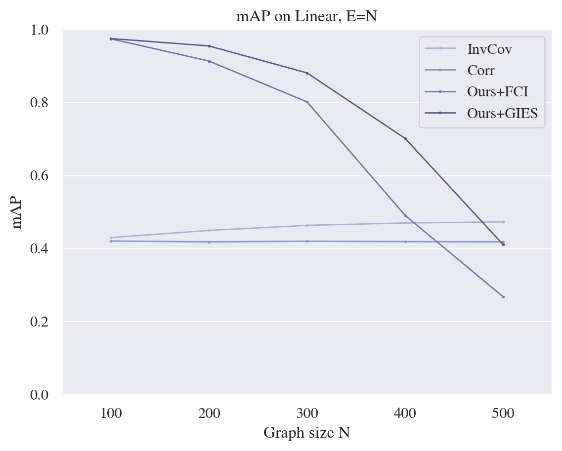
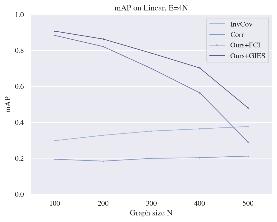
Figure 9: mAP on graphs larger than seen during training. Due to an insufficient maximum number of subset embeddings, we were only able to sample 500 batches, which appears to be too few for larger graphs. These values correspond to the numbers in Table 10.

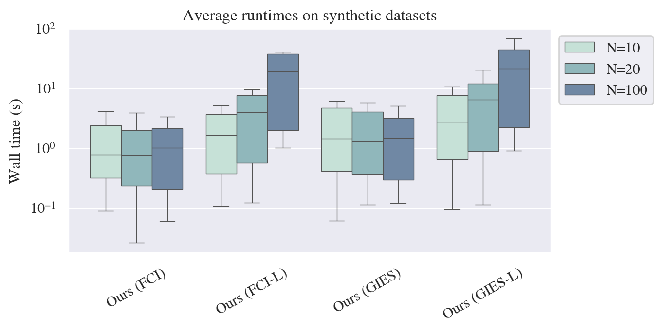
Figure 10: Runtime for heuristics-based greedy sampler vs. model uncertainty-based greedy sampler (suffix -l). For sampling, the model was run on CPU only, due to the difficulty of invoking GPU in the PyTorch data sampler.

References

- Bommasani et al. (2022) Bommasani, R., Hudson, D. A., Adeli, E., Altman, R., Arora, S., von Arx, S., Bernstein, M. S., Bohg, J., Bosselut, A., Brunskill, E., Brynjolfsson, E., Buch, S., Card, D., Castellon, R., Chatterji, N., Chen, A., Creel, K., Davis, J. Q., Demszky, D., Donahue, C., Doumbouya, M., Durmus, E., Ermon, S., Etchemendy, J., Ethayarajh, K., Fei-Fei, L., Finn, C., Gale, T., Gillespie, L., Goel, K., Goodman, N., Grossman, S., Guha, N., Hashimoto, T., Henderson, P., Hewitt, J., Ho, D. E., Hong, J., Hsu, K., Huang, J., Icard, T., Jain, S., Jurafsky, D., Kalluri, P., Karamcheti, S., Keeling, G., Khani, F., Khattab, O., Koh, P. W., Krass, M., Krishna, R., Kuditipudi, R., Kumar, A., Ladhak, F., Lee, M., Lee, T., Leskovec, J., Levent, I., Li, X. L., Li, X., Ma, T., Malik, A., Manning, C. D., Mirchandani, S., Mitchell, E., Munyikwa, Z., Nair, S., Narayan, A., Narayanan, D., Newman, B., Nie, A., Niebles, J. C., Nilforoshan, H., Nyarko, J., Ogut, G., Orr, L., Papadimitriou, I., Park, J. S., Piech, C., Portelance, E., Potts, C., Raghunathan, A., Reich, R., Ren, H., Rong, F., Roohani, Y., Ruiz, C., Ryan, J., Ré, C., Sadigh, D., Sagawa, S., Santhanam, K., Shih, A., Srinivasan, K., Tamkin, A., Taori, R., Thomas, A. W., Tramèr, F., Wang, R. E., Wang, W., Wu, B., Wu, J., Wu, Y., Xie, S. M., Yasunaga, M., You, J., Zaharia, M., Zhang, M., Zhang, T., Zhang, X., Zhang, Y., Zheng, L., Zhou, K., and Liang, P. On the opportunities and risks of foundation models, 2022.
- Bradley (1997) Bradley, A. P. The use of the area under the roc curve in the evaluation of machine learning algorithms. Pattern Recognition, 30(7):1145–1159, 1997. ISSN 0031-3203. doi: https://doi.org/10.1016/S0031-3203(96)00142-2.
- Brouillard et al. (2020) Brouillard, P., Lachapelle, S., Lacoste, A., Lacoste-Julien, S., and Drouin, A. Differentiable causal discovery from interventional data, 2020.
- Brown et al. (2020) Brown, T. B., Mann, B., Ryder, N., Subbiah, M., Kaplan, J., Dhariwal, P., Neelakantan, A., Shyam, P., Sastry, G., Askell, A., Agarwal, S., Herbert-Voss, A., Krueger, G., Henighan, T., Child, R., Ramesh, A., Ziegler, D. M., Wu, J., Winter, C., Hesse, C., Chen, M., Sigler, E., Litwin, M., Gray, S., Chess, B., Clark, J., Berner, C., McCandlish, S., Radford, A., Sutskever, I., and Amodei, D. Language models are few-shot learners, 2020.
- Bühlmann et al. (2014) Bühlmann, P., Peters, J., and Ernest, J. CAM: Causal additive models, high-dimensional order search and penalized regression. The Annals of Statistics, 42(6):2526 – 2556, 2014. doi: 10.1214/14-AOS1260.
- Chickering (2002) Chickering, D. M. Optimal structure identification with greedy search. 3:507–554, November 2002.
- Dibaeinia & Sinha (2020) Dibaeinia, P. and Sinha, S. Sergio: A single-cell expression simulator guided by gene regulatory networks. Cell Systems, 11(3):252–271.e11, 2020. ISSN 2405-4712. doi: https://doi.org/10.1016/j.cels.2020.08.003.
- Geffner et al. (2022) Geffner, T., Antoran, J., Foster, A., Gong, W., Ma, C., Kiciman, E., Sharma, A., Lamb, A., Kukla, M., Pawlowski, N., Allamanis, M., and Zhang, C. Deep end-to-end causal inference, 2022.
- Glymour et al. (2019) Glymour, C., Zhang, K., and Spirtes, P. Review of causal discovery methods based on graphical models. Frontiers in Genetics, 10, 2019. ISSN 1664-8021. doi: 10.3389/fgene.2019.00524.
- Guo et al. (2017) Guo, C., Pleiss, G., Sun, Y., and Weinberger, K. Q. On calibration of modern neural networks. In International Conference on Machine Learning, 2017.
- Hauser & Bühlmann (2012) Hauser, A. and Bühlmann, P. Characterization and greedy learning of interventional markov equivalence classes of directed acyclic graphs. 2012.
- Ho et al. (2020) Ho, J., Kalchbrenner, N., Weissenborn, D., and Salimans, T. Axial attention in multidimensional transformers, 2020.
- Hornik et al. (1989) Hornik, K., Stinchcombe, M., and White, H. Multilayer feedforward networks are universal approximators. Neural Networks, 2(5):359–366, 1989. ISSN 0893-6080. doi: https://doi.org/10.1016/0893-6080(89)90020-8.
- Huang et al. (2020) Huang, B., Zhang, K., Zhang, J., Ramsey, J., Sanchez-Romero, R., Glymour, C., and Schölkopf, B. Causal discovery from heterogeneous/nonstationary data with independent changes, 2020.
- Hägele et al. (2023) Hägele, A., Rothfuss, J., Lorch, L., Somnath, V. R., Schölkopf, B., and Krause, A. Bacadi: Bayesian causal discovery with unknown interventions, 2023.
- Kalainathan et al. (2020) Kalainathan, D., Goudet, O., and Dutta, R. Causal discovery toolbox: Uncovering causal relationships in python. Journal of Machine Learning Research, 21(37):1–5, 2020.
- Lachapelle et al. (2020) Lachapelle, S., Brouillard, P., Deleu, T., and Lacoste-Julien, S. Gradient-based neural dag learning, 2020.
- Lam et al. (2022) Lam, W.-Y., Andrews, B., and Ramsey, J. Greedy relaxations of the sparsest permutation algorithm. In Cussens, J. and Zhang, K. (eds.), Proceedings of the Thirty-Eighth Conference on Uncertainty in Artificial Intelligence, volume 180 of Proceedings of Machine Learning Research, pp. 1052–1062. PMLR, 01–05 Aug 2022.
- Ledoit & Wolf (2004) Ledoit, O. and Wolf, M. A well-conditioned estimator for large-dimensional covariance matrices. Journal of Multivariate Analysis, 88(2):365–411, 2004. ISSN 0047-259X. doi: https://doi.org/10.1016/S0047-259X(03)00096-4.
- Lippe et al. (2022) Lippe, P., Cohen, T., and Gavves, E. Efficient neural causal discovery without acyclicity constraints. In International Conference on Learning Representations, 2022.
- Lopez et al. (2022) Lopez, R., Hütter, J.-C., Pritchard, J. K., and Regev, A. Large-scale differentiable causal discovery of factor graphs. In Advances in Neural Information Processing Systems, 2022.
- Loshchilov & Hutter (2019) Loshchilov, I. and Hutter, F. Decoupled weight decay regularization, 2019.
- Löwe et al. (2022) Löwe, S., Madras, D., Zemel, R., and Welling, M. Amortized causal discovery: Learning to infer causal graphs from time-series data, 2022.
- Monti et al. (2019) Monti, R. P., Zhang, K., and Hyvarinen, A. Causal discovery with general non-linear relationships using non-linear ica, 2019.
- Mooij et al. (2020) Mooij, J. M., Magliacane, S., and Claassen, T. Joint causal inference from multiple contexts. 2020.
- Pérez et al. (2019) Pérez, J., Marinković, J., and Barceló, P. On the turing completeness of modern neural network architectures. In International Conference on Learning Representations, 2019.
- Radford et al. (2021) Radford, A., Kim, J. W., Hallacy, C., Ramesh, A., Goh, G., Agarwal, S., Sastry, G., Askell, A., Mishkin, P., Clark, J., Krueger, G., and Sutskever, I. Learning transferable visual models from natural language supervision, 2021.
- Rao et al. (2021) Rao, R. M., Liu, J., Verkuil, R., Meier, J., Canny, J., Abbeel, P., Sercu, T., and Rives, A. Msa transformer. In Meila, M. and Zhang, T. (eds.), Proceedings of the 38th International Conference on Machine Learning, volume 139 of Proceedings of Machine Learning Research, pp. 8844–8856. PMLR, 18–24 Jul 2021.
- Reizinger et al. (2023) Reizinger, P., Sharma, Y., Bethge, M., Schölkopf, B., Huszár, F., and Brendel, W. Jacobian-based causal discovery with nonlinear ICA. Transactions on Machine Learning Research, 2023. ISSN 2835-8856.
- Replogle et al. (2022) Replogle, J. M., Saunders, R. A., Pogson, A. N., Hussmann, J. A., Lenail, A., Guna, A., Mascibroda, L., Wagner, E. J., Adelman, K., Lithwick-Yanai, G., Iremadze, N., Oberstrass, F., Lipson, D., Bonnar, J. L., Jost, M., Norman, T. M., and Weissman, J. S. Mapping information-rich genotype-phenotype landscapes with genome-scale Perturb-seq. Cell, 185(14):2559–2575, Jul 2022.
- Sachs et al. (2005) Sachs, K., Perez, O., Pe’er, D., Lauffenburger, D. A., and Nolan, G. P. Causal protein-signaling networks derived from multiparameter single-cell data. Science, 308(5721):523–529, 2005. doi: 10.1126/science.1105809.
- Sanchez et al. (2023) Sanchez, P., Liu, X., O’Neil, A. Q., and Tsaftaris, S. A. Diffusion models for causal discovery via topological ordering. In The Eleventh International Conference on Learning Representations, ICLR 2023, Kigali, Rwanda, May 1-5, 2023. OpenReview.net, 2023.
- Schaeffer et al. (2023) Schaeffer, R., Miranda, B., and Koyejo, O. Are emergent abilities of large language models a mirage? Advances in Neural Information Processing Systems, abs/2304.15004, 2023.
- Schwarz (1978) Schwarz, G. Estimating the Dimension of a Model. The Annals of Statistics, 6(2):461 – 464, 1978. doi: 10.1214/aos/1176344136.
- Shimizu et al. (2006) Shimizu, S., Hoyer, P. O., Hyvarinen, A., and Kerminen, A. A linear non-gaussian acyclic model for causal discovery. Journal of Machine Learning Research, 7(72):2003–2030, 2006.
- Spirtes et al. (1990) Spirtes, P., Glymour, C., and Scheines, R. Causality from probability. In Conference Proceedings: Advanced Computing for the Social Sciences, 1990.
- Spirtes et al. (1995) Spirtes, P., Meek, C., and Richardson, T. Causal inference in the presence of latent variables and selection bias. In Proceedings of the Eleventh Conference on Uncertainty in Artificial Intelligence, UAI’95, pp. 499–506, San Francisco, CA, USA, 1995. Morgan Kaufmann Publishers Inc. ISBN 1558603859.
- Spirtes et al. (2001) Spirtes, P., Glymour, C., and Scheines, R. Causation, Prediction, and Search. MIT Press, 2001. doi: https://doi.org/10.7551/mitpress/1754.001.0001.
- Sz’ekely et al. (2007) Sz’ekely, G. J., Rizzo, M. L., and Bakirov, N. K. Measuring and testing dependence by correlation of distances. Annals of Statistics, 35:2769–2794, 2007.
- Tsamardinos et al. (2006) Tsamardinos, I., Brown, L. E., and Aliferis, C. F. The max-min hill-climbing bayesian network structure learning algorithm. Machine learning, 65(1):31–78, 2006.
- Verma & Pearl (1990) Verma, T. S. and Pearl, J. On the equivalence of causal models. In Proceedings of the Sixth Conference on Uncertainty in Artificial Intelligence, 1990.
- Yun et al. (2019) Yun, C., Bhojanapalli, S., Rawat, A. S., Reddi, S. J., and Kumar, S. Are transformers universal approximators of sequence-to-sequence functions? CoRR, abs/1912.10077, 2019.
- Zhang et al. (2023) Zhang, J., Jennings, J., Zhang, C., and Ma, C. Towards causal foundation model: on duality between causal inference and attention, 2023.
- Zhang & Hyvarinen (2012) Zhang, K. and Hyvarinen, A. On the identifiability of the post-nonlinear causal model, 2012.
- Zheng et al. (2018) Zheng, X., Aragam, B., Ravikumar, P., and Xing, E. P. Dags with no tears: Continuous optimization for structure learning, 2018.
- Zheng et al. (2023) Zheng, Y., Huang, B., Chen, W., Ramsey, J., Gong, M., Cai, R., Shimizu, S., Spirtes, P., and Zhang, K. Causal-learn: Causal discovery in python. arXiv preprint arXiv:2307.16405, 2023.