A General Framework for
Learning from Weak Supervision

Hao Chen¹ haoc3@andrew.cmu.edu ¹Carnegie Mellon University, ²Microsoft Research Asia, ³Nanyang Technological University,
⁴Peiking University, ⁵RIKEN AIP, ⁶The University of Tokyo, ⁷Mohamed bin Zayed University of AI Jindong Wang² ¹Carnegie Mellon University, ²Microsoft Research Asia, ³Nanyang Technological University,
⁴Peiking University, ⁵RIKEN AIP, ⁶The University of Tokyo, ⁷Mohamed bin Zayed University of AI Lei Feng³ ¹Carnegie Mellon University, ²Microsoft Research Asia, ³Nanyang Technological University,
⁴Peiking University, ⁵RIKEN AIP, ⁶The University of Tokyo, ⁷Mohamed bin Zayed University of AI Xiang Li¹ ¹Carnegie Mellon University, ²Microsoft Research Asia, ³Nanyang Technological University,
⁴Peiking University, ⁵RIKEN AIP, ⁶The University of Tokyo, ⁷Mohamed bin Zayed University of AI Yidong Wang⁴ ¹Carnegie Mellon University, ²Microsoft Research Asia, ³Nanyang Technological University,
⁴Peiking University, ⁵RIKEN AIP, ⁶The University of Tokyo, ⁷Mohamed bin Zayed University of AI
Xing Xie² ¹Carnegie Mellon University, ²Microsoft Research Asia, ³Nanyang Technological University,
⁴Peiking University, ⁵RIKEN AIP, ⁶The University of Tokyo, ⁷Mohamed bin Zayed University of AI Masashi Sugiyama^5,6 ¹Carnegie Mellon University, ²Microsoft Research Asia, ³Nanyang Technological University,
⁴Peiking University, ⁵RIKEN AIP, ⁶The University of Tokyo, ⁷Mohamed bin Zayed University of AI Rita Singh¹ ¹Carnegie Mellon University, ²Microsoft Research Asia, ³Nanyang Technological University,
⁴Peiking University, ⁵RIKEN AIP, ⁶The University of Tokyo, ⁷Mohamed bin Zayed University of AI Bhiksha Raj^1,7 ¹Carnegie Mellon University, ²Microsoft Research Asia, ³Nanyang Technological University,
⁴Peiking University, ⁵RIKEN AIP, ⁶The University of Tokyo, ⁷Mohamed bin Zayed University of AI

Abstract

Weakly supervised learning generally faces challenges in applicability to various scenarios with diverse weak supervision and in scalability due to the complexity of existing algorithms, thereby hindering the practical deployment. This paper introduces a general framework for learning from weak supervision (GLWS) with a novel algorithm. Central to GLWS is an Expectation-Maximization (EM) formulation, adeptly accommodating various weak supervision sources, including instance partial labels, aggregate statistics, pairwise observations, and unlabeled data. We further present an advanced algorithm that significantly simplifies the EM computational demands using a Non-deterministic Finite Automaton (NFA) along with a forward-backward algorithm, which effectively reduces time complexity from quadratic or factorial often required in existing solutions to linear scale. The problem of learning from arbitrary weak supervision is therefore converted to the NFA modeling of them. GLWS not only enhances the scalability of machine learning models but also demonstrates superior performance and versatility across 11 weak supervision scenarios. We hope our work paves the way for further advancements and practical deployment in this field.

1 Introduction

Over the past few years, machine learning models have shown promising performance in virtually every aspect of our lives (Radford et al., 2021; Rombach et al., 2022; Dehghani et al., 2023; OpenAI, 2023). This success is typically attributed to large-scale and high-quality training data with complete and accurate supervision. However, obtaining such precise labels in realistic applications is often prohibitive due to various factors, such as the cost of annotation (Settles et al., 2008; Gadre et al., 2023), the biases and subjectivity of annotators (Tommasi et al., 2017; Pagano et al., 2023), and privacy concerns (Mireshghallah et al., 2020; Strobel and Shokri, 2022). The resulting incomplete, inexact, and inaccurate forms of supervision are typically referred to as weak supervision (Zhou, 2018; Sugiyama et al., 2022).

Refer to caption — Figure 1: Average performance overview of the proposed method on 11 common weak supervision settings, compared to previous best methods (margins shown on the top of bars). GLWS is capable of learning from any weak supervision universally and effectively.

Previous literature has explored numerous configurations of weak supervision problems, including learning from sets of instance label candidates (Luo and Orabona, 2010; Cour et al., 2011; Ishida et al., 2019; Feng et al., 2020a, b; Wang et al., 2022a; Wu et al., 2022), aggregate group statistics (Maron and Lozano-Pérez, 1997; Zhou, 2004; Kück and de Freitas, 2005; Quadrianto et al., 2008; Ilse et al., 2018; Zhang et al., 2020; Scott and Zhang, 2020; Zhang et al., 2022), pairwise observations (Bao et al., 2018, 2020; Feng et al., 2021; Cao et al., 2021a; Wang et al., 2023a), and unlabeled data (Lu et al., 2018; Sohn et al., 2020; Shimada et al., 2021; Wang et al., 2022b; Tang et al., 2023). More recently, some efforts have been made to design versatile techniques that can handle multiple settings simultaneously (Van Rooyen and Williamson, 2018; Zhang et al., 2020; Chiang and Sugiyama, 2023; Shukla et al., 2023; Wei et al., 2023).

Despite the prosperous developments in various settings, we identify two challenges that impede the practical application of these weakly supervised methods. First, designing a method capable of universally handling all configurations remains difficult. The variation in forms of weak supervision often necessitates specialized and tailored solutions (Ilse et al., 2018; Yan et al., 2018; Yang et al., 2022; Zhang et al., 2022; Scott and Zhang, 2020). Even recent versatile solutions are limited in their applicability to certain contexts (Shukla et al., 2023; Wei et al., 2023). Second, prior works typically exhibit limited scalability in realistic problems due to oversimplifications and unfavorable modeling complexity. Some methods assume conditional independence of instances for aggregate observations (Van Rooyen and Williamson, 2018; Cui et al., 2020; Zhang et al., 2020; Wei et al., 2023), making them unsuitable for handling long sequence data prevalent in practical scenarios. Moreover, despite such simplifications, they still require infeasible computational complexity, either quadratic (Shukla et al., 2023) or factorial (Wei et al., 2023), to address specific weak supervision configurations.

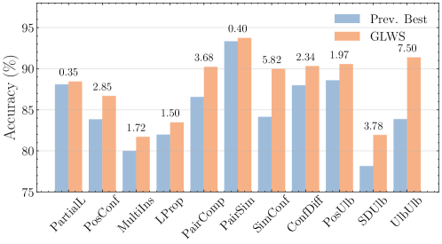
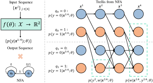
To overcome these challenges and effectively apply weakly supervised learning in real-world scenarios, we propose a general framework and a novel algorithm that allows efficient learning from arbitrary weak supervision, termed as GLWS, as in the results demonstrated in Figure 1. At the core of GLWS is an Expectation-Maximization (EM) (Dempster et al., 1977) learning objective formulation for weak supervision, and a forward-backward algorithm (Rabiner, 1989; Graves et al., 2006) designed to solve the EM in linear time by representing arbitrary form of weak supervision as a Non-deterministic Finite Automaton (NFA) (Rabin and Scott, 1959). More specifically, to train a classification model with learnable parameters $\theta$ on weak supervision, denoted abstractly as $W$ , we treat the ground truth label $Y$ as a missing latent variable and maximize the log-likelihood of joint input $X$ and $W$ : $\log P(X,W;\theta)=\log\sum_{Y}P(X,W;\theta)P(Y|X,W;\theta)$ . As $P(Y|X,W;\theta)$ is unknown before determining $\theta$ , solving the problem usually requires iterative hill-climbing solutions. Therefore, we employ the widely used EM algorithm, which iteratively maximizes the expectation of the log-likelihood $\mathbb{E}_{Y|X,W;\theta^{t}}[\log P(X,W,Y;\theta)]$ at time step $t$ . It leads to two training objectives: an unsupervised instance consistency term $\mathbb{E}_{Y|X,W;\theta^{t}}[\log P(Y|X;\theta)]$ that encourages the prediction to be consistent with the labeling distribution imposed by $W$ , and a supervised objective $\log P(W|Y,X;\theta)$ that fosters the group predictions fulfilling $W$ . We further propose a novel perspective to perform the EM formulation. Without loss of generality, we treat both the inputs and the precise labels as sequence¹¹1For aggregate and pairwise observations, the inputs are naturally sequences of instances. The inputs can be viewed as permutation-invariant sequences at the batch (dataset) level for weak supervision of partial labels and unlabeled data. The same applies to the precise labels and predictions from the model.. Thus, the problem of identifying all possible labelings is converted into assigning labels/symbols to the input sequence in a manner that adheres to $W$ . This process can be effectively modeled using an NFA (Rabin and Scott, 1959), where the finite set of states and transition is dictated by $W$ , and the finite set of symbols corresponds to $Y$ . The EM learning objectives can then be computed efficiently in linear time using a forward-backward algorithm on the trellis expanded from the NFA and model’s predictions. An overview is shown in Figure 2.

While this is not the first EM perspective of weak supervision (Denœux, 2011; Quost and Denoeux, 2016; Wang et al., 2022a; Wei et al., 2023), GLWS distinguishes from prior arts in solving the complete EM efficiently and practically. Compared to the recent efforts towards the unification of weak supervision, our method neither relies on the aforementioned conditional independence assumption as in Wei et al. (2023) nor involves approximation of EM as in Wang et al. (2022a); Shukla et al. (2023) that solves the supervised term of EM only. Our contributions can be summarized as:

•

We propose an EM framework that accommodates weak supervision of arbitrary forms, leading to two learning objectives, as a generalization of the prior arts.
•

We design a forward-backward algorithm that performs the EM by treating weak supervision as an NFA. The EM can thus be computed via iterative forward-backward pass on the trellis expanded from the NFA in linear time.
•

On 11 weak supervision settings, the proposed method consistently achieves the state-of-the-art performance, demonstrating its universality and effectiveness. The codebase covering all these settings will be released²²2https://github.com/Hhhhhhao/General-Framework-Weak-Supervision.

2 Related Work

2.1 Learning from Weak Supervision

Various problems for learning from weak supervision have been extensively studied in the past, and we categorize them into four broad categories: instance label candidates, aggregate observations, pairwise observations, and unlabeled data. Learning from instance label candidates, also known as partial label (PartialL) or complementary label (CompL) learning (Cour et al., 2011; Luo and Orabona, 2010; Feng et al., 2020c; Wang et al., 2019; Wen et al., 2021; Wu et al., 2022; Wang et al., 2022a; Ishida et al., 2019; Feng et al., 2020a), involves weak supervision as a set of label candidates, either containing or complementary to the ground truth label for each instance. Aggregate observation assumes supervision over a group of instances (Zhang et al., 2020), with multiple instances (MultiIns) learning (Maron and Lozano-Pérez, 1997; Ilse et al., 2018) and label proportion (LProp) learning (Quadrianto et al., 2008; Scott and Zhang, 2020; Zhang et al., 2022) as common examples. The weak supervision here usually denotes statistics over a group of instances. Pairwise observation, a special case of aggregate observation, deals with pairs of instances. Pairwise comparison (Pcomp) (Feng et al., 2021) and pairwise similarity (PSim) (Bao et al., 2018; Zhang et al., 2020), along with more recent developments such as similarity confidence (SimConf) (Cao et al., 2021a) and confidence difference (ConfDiff) (Wang et al., 2023a), fall into this category. Similarity, comparison, confidence scores, and relationships from the pre-trained models are usually adopted as weak supervision for pairwise observations. The fourth category, unlabeled data, is often supplemented by the labeled dataset as the weak supervision in this setting, which is sometimes complemented by the class’s prior information. Semi-supervised learning (SemiSL) (Sohn et al., 2020; Xie et al., 2020; Zhang et al., 2021; Wang et al., 2023b; Chen et al., 2023), positive unlabeled (PosUlb) learning (du Plessis et al., 2015; Hammoudeh and Lowd, 2020; Chen et al., 2020; Garg et al., 2021; Kiryo et al., 2017; Zhao et al., 2022), similarity dissimilarity unlabeled (SDUlb) learning (Shimada et al., 2021), and Unlabeled unlabeled (UlbUlb) learning (Lu et al., 2018; Tang et al., 2023) fall into this category. Our framework is capable of addressing and unifying these diverse categories.

2.2 Towards the Unification of Weak Supervision

Although researchers have invested significant efforts in finding solutions to different forms of weak supervision, the practical unification of these problems still remains a distant goal. PosUlb, SDUlb, and UlbUlb learning can be connected to each other by substituting parameters (Lu et al., 2018; Feng et al., 2021). Zhang et al. (2020) have developed a probabilistic framework for pairwise (Hsu et al., 2019) and triplet comparison (Cui et al., 2020). Shukla et al. (2023) proposed a unified solution for weak supervision involving count statistics. They used a dynamic programming method over the aggregate observation to compute and maximize the count loss of $P(W|Y,X;\theta)$ , corresponding to the supervised term in our EM formulation. The computational complexity is thus quadratic to the group length since the proposed dynamic programming algorithm iterates through the entire group. Wei et al. (2023) introduced the universal unbiased method (UUM) for aggregate observation, which is also interpretable from the EM perspective. Based on the assumptions of conditional independence of instances within a group and weak supervision given true labels, Wei et al. (2023) derived closed-form objectives for MultiIns, LProp, and PSim settings. However, the oversimplification of conditional independence limits UUM’s scalability, particularly for LProp learning with long sequences. Chiang and Sugiyama (2023) provided a comprehensive risk analysis for various types of weak supervision from the perspective of the contamination matrix. Our framework offers a versatile and scalable solution, capable of efficiently handling a wider range of weak supervision without the limitations imposed by oversimplifications or computational complexity.

3 Method

In this section, we introduce our proposed framework and algorithm for learning from arbitrary weak supervision (GLWS). GLWS is based on the EM formulation (Dempster et al., 1977), where we consider the precise labels as the latent variable. We introduce an NFA (Rabin and Scott, 1959) modeling of weak supervision, which allows us to compute EM using the forward-backward algorithm in linear time.

3.1 Preliminaries

Let $\mathbf{x}\in\mathcal{X}$ be a training instance and $y\in\mathcal{Y}$ the corresponding precise supervision, where the input space $\mathcal{X}\subset\mathbb{R}^{D}$ has $D$ dimensions, and the label space $\mathcal{Y}=[K-1]:=\{0,1,\dots,K-1\}$ encompasses a total of $K$ classes. In fully supervised learning, the training dataset with complete and precise annotations is defined as $\mathcal{D}=\{(\mathbf{x}_{i},y_{i})\}_{i\in[N]}$ and consists of $N$ samples. Assume that each training example $(\mathbf{x},y)$ is identically and independently sampled from the joint distribution $p(\mathbf{x},y)$ . The classifier $f(\theta):\mathcal{X}\rightarrow\mathbb{R}^{K}$ predicts $p(y|\mathbf{x};\theta)$ with learnable parameters $\theta$ , and is trained to maximize the log-likelihood $\log P(X,Y;\theta)$ :

\theta^{*}=\operatorname*{arg\,max}_{\theta}\log P(X,Y;\theta).

(1)

This process results in the cross-entropy (CE) loss function:

\mathcal{L}_{\mathrm{Full}}=\sum_{i=1}^{N}\sum_{k=0}^{K}-\mathbbm{1}[y_{i}=k]\log p(y_{i}|\mathbf{x}_{i};\theta).

(2)

3.2 General Framework for Weak Supervision

In practice, we may not have fully accessible precise supervision, i.e., $Y$ is unknown. Instead, we may encounter various types of weak supervision for training instances, e.g., instance-wise label candidates, aggregated count statistics, pairwise similarity, unlabeled data, etc. We define weak supervision abstractly as $W$ , representing an arbitrary form of information given to the training instances. For example, in PartialL (Feng et al., 2020b; Wang et al., 2022a; Wu et al., 2022), $W$ is given as a set of label candidates for each instance $\mathcal{S}\subseteq\mathcal{Y}$ . In MultiIns (Maron and Lozano-Pérez, 1997; Zhou, 2004) and LProp learning (Yu et al., 2014) that deals with aggregate observations, $W$ is given as the count statistics for each label $\{\sum_{j=1}^{L}\mathbbm{1}[y^{j}=k]\geq 1\mid\forall k\in\mathcal{Y}\}$ and $\{\sum_{j=1}^{L}\mathbbm{1}[y^{j}=k]\mid\forall k\in\mathcal{Y}\}$ over a group of $L$ instances $\{\mathbf{x}^{j}\}_{j\in[L]}$ ³³3We use $\mathbf{x}_{i}$ ( $y_{i}$ ) to denote an instance/group in dataset of size $N$ , and $\mathbf{x}^{j}$ ( $y^{j}$ ) to denote an instance in the group $\{\mathbf{x}^{j}\}_{j\in[L]}$ of size $L$ . Each $\mathbf{x}_{i}$ ( $y_{i}$ ) in the dataset can denote a group with $L\geq 1$ ., respectively. When $W$ represents the precise labels, it recovers fully supervised learning. With $W$ , we must estimate the model to maximize the likelihood of the data $X$ and the information $W$ we have been provided:

\theta^{*}=\operatorname*{arg\,max}_{\theta}\log P(X,W;\theta)=\operatorname*{arg\,max}_{\theta}\sum\nolimits_{Y}\log P(X,W,Y;\theta).

(3)

As $Y$ is unknown and the marginalization over $Y$ requires $\theta$ , it is infeasible to solve Equation 3 in a closed form, and instead typically needs the iterative hill-climbing solutions like EM algorithm. Thus, the maximum log-likelihood estimation in Equation 3 can be solved by iteratively maximizing the variational lower bound of the log-likelihood $\log P(X,W,Y;\theta)$ :

\theta^{t+1}=\operatorname*{arg\,max}_{\theta}\mathbb{E}_{Y|X,W;\theta^{t}}\left[\log P(X,W,Y;\theta)\right],

(4)

where $\theta^{t}$ denotes the $t$ -th estimation of $\theta$ . $P(Y|X,W;\theta^{t})$ represents a distribution on all possible labelings imposed by $W$ with $\theta^{t}$ . The log-likelihood is then maximized on the expectation over the distribution of all possible labelings. The derivation of Equation 4 is provided in Section A.1.

To derive the loss function for arbitrary weak supervision that includes instance-level and group-level $W$ from Equation 4, without loss of generality, we treat the realization of training instances $X$ and the corresponding true precise labels $Y$ all as sequence: $\mathbf{x}^{1:L}=\{\mathbf{x}^{j}\}_{j\in[L]}$ and $y^{1:L}=\{y^{j}\}_{j\in[L]}$ of size $L$ and $L$ could be 1. We also treat different types of weak supervision $w\in W$ as the information given for the input sequence. The sequence can be naturally formed from a batch of training samples, an aggregate observation, or a pairwise observation. Each instance in the dataset is thus generalized to $\mathbf{x}_{i}\rightarrow\mathbf{x}_{i}^{1:L}$ with $L\geq 1$ . We make the following assumption, which almost always holds in reality:

Assumption 3.1.

The sequence of predictions on precise labels $y^{1:L}$ is conditionally independent given the whole sequence of inputs $\mathbf{x}^{1:L}$ , i.e., $p(y^{1:L}|\mathbf{x}^{1:L})=\prod_{j}^{L}p(y^{j}|\mathbf{x}^{1:L})$ .

This notation allows us to deal with different weak supervision for both instance and group/bag data more flexibly.

Proposition 3.2.

For weakly supervised learning problems, the training objectives can be derived from Equation 4 as:

\begin{split}&\mathcal{L}_{\mathrm{Weak}}=\mathcal{L}_{\mathrm{U}}+\mathcal{L}_{\mathrm{S}},\\ &\mathcal{L}_{\mathrm{U}}=\sum_{i=1}^{N}\sum_{j=1}^{L}-p(y_{i}^{j}|\mathbf{x}^{1:L}_{i},w_{i};\theta^{t})\log p(y_{i}^{j}|\mathbf{x}^{j}_{i};\theta),\\ &\mathcal{L}_{\mathrm{S}}=\sum_{i}^{N}-\log p(w_{i}|\mathbf{x}_{i}^{1:L},y_{i}^{1:L};\theta).\end{split}

(5)

The detailed derivation of Equation 5 is shown in Section A.2. Equation 5 consists of two parts: an unsupervised loss $\mathcal{L}_{\mathrm{U}}$ that encourages the instance-wise predictions from the classifier to align with the probability of this prediction given all possible labelings imposed by $W$ , and a supervised loss $\mathcal{L}_{\mathrm{S}}$ that encourages the sequence predictions to fulfill $W$ .

3.3 Weak Supervision as NFA

Although the proposed EM formulation can deal with various types of weak supervision flexibly, it is still computational intensive to calculate the probability $p(y^{j}|\mathbf{x}^{1:L},w;\theta)$ and $p(w|y^{1:L},\mathbf{x}^{1:L};\theta)$ for all possible labelings imposed by the given weak supervision. For example, in LProp learning where $W$ is the label count over a group of $L$ instances, the complexity of finding all possible labelings is of factorial $\mathcal{O}(L!)$ . In most cases, the complexity is of exponential $\mathcal{O}(K^{L})$ where $K$ is the total number of classes. Moreover, while some recent methods towards unification can also be related to the proposed EM formulation (Shukla et al., 2023; Wei et al., 2023), they both involve a certain degree of simplification to approximate the complete EM formulation, which limits their scalability, as discussed in Section 2.2. Our method notably distinguishes from the prior arts in that we tackle weak supervision with the complete EM.

Here, we present a novel perspective to overcome the infeasibility of computing the complete EM. Under the sequential view, we treat the problem of assigning labels $\{y^{j}\}_{j\in[L]}$ to inputs $\{\mathbf{x}^{j}\}_{j\in[L]}$ as generating a sequence of symbols $y^{1:L}$ to $\mathbf{x}^{1:L}$ fulfilling $W$ . For simplicity, we only consider binary classification problems here. In Section 3.5, we will show the generalization to multi-class classification problems. This process naturally fits the mechanism of the NFA (Rabin and Scott, 1959). We can thus model weak supervision $W$ as an NFA that defines a set of finite states and transition rules, summarizing all possible labelings imposed by $W$ .

Definition 3.3.

(Rabin and Scott, 1959) A Non-deterministic Finite Automaton (NFA) is defined as a tuple ( $Q$ , $\Sigma$ , $\delta$ , $q_{0}$ , $F$ ), where $Q$ is a finite set of states, $\Sigma$ is a finite set of symbols, $\delta$ is a transition function $Q\times\Sigma\rightarrow P(Q)$ , $q_{0}\in Q$ is the initial state, and $F\subseteq Q$ is a set of accepting states.

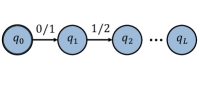
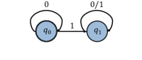
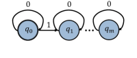
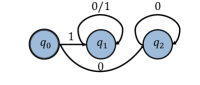
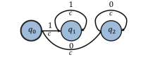
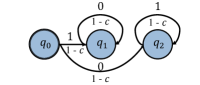
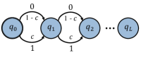
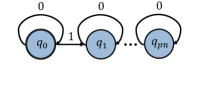
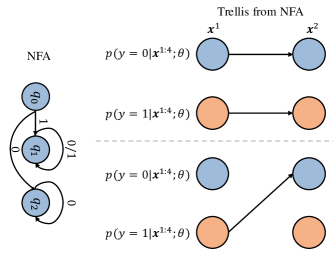
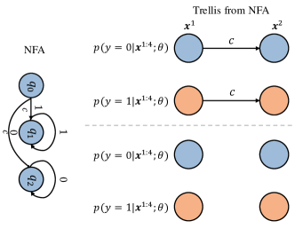
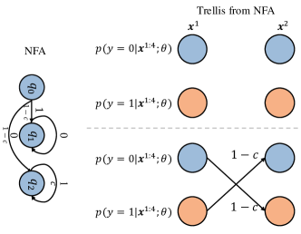
We define the NFA of weak supervision $W$ similarly, with states $Q$ , initial state $q_{0}$ , and accepting states $F$ determined by $W$ , symbols $\Sigma=\mathcal{Y}=\{0,1\}$ , and a transition function $\delta$ defining the possible transitions between states. We can now represent all possible labelings imposed by $W$ as the language accepted by the NFA: $\{y^{1:L}|\delta(q_{0},y^{1:L})\in F\}$ . The problem of finding all possible labelings is thereby converted to modeling the NFA of different types of weak supervision. We present the modeling of NFA for common forms of $W$ in Figure 3. For example, in MultiIns learning (Figure 3(b)) with $W$ denoting at least one positive sample within a group instance, its NFA contains 2 states $Q=\{q_{0},q_{1}\}$ . The initial state $q_{0}$ can only transit to the accepting state $q_{1}$ via symbol $1$ to ensure $W$ is satisfied. Once reaching $q_{1}$ , transit via $0$ and $1$ are both allowed. For LProp with $m$ positive labels (Figure 3(c)), its NFA must transit via 1 for $m$ times from $q_{0}$ to $q_{m}$ to satisfy $W$ , resulting in $m+1$ states.

3.4 The Forward-Backward Algorithm

We are now set to compute the EM formulation with NFA.

Proposition 3.4.

Given the inputs $\mathbf{x}^{1:L}$ , we treat the outputs sequence from the classifier $p(y^{1:L}|\mathbf{x}^{1:L};\theta)$ as a linear chain graph. By taking the product on the linear chain graph of $p(y^{1:L}|\mathbf{x}^{1:L};\theta)$ and the NFA graph of $W$ , we obtain the trellis in the resulting graph as possible labelings.

We have $p(y^{j}|\mathbf{x}^{1:L},w;\theta^{t})\propto p(y^{j},w|\mathbf{x}^{1:L};\theta^{t})$ from Bayes’ theorem, where the latter denotes the total probability of all valid labelings that go through $y^{j}$ , and $p(w|y^{1:L},\mathbf{x}^{1:L};\theta)$ in Equation 5 denotes the total probability from accepting states of the resulting graph. Fortunately, both the probability of $p(y^{j},w|\mathbf{x}^{1:L};\theta^{t})$ and $p(w|y^{1:L},\mathbf{x}^{1:L};\theta)$ can be computed in linear time to the sequence length with dynamic programming on the trellis of the resulting graph, specifically the forward-backward algorithm (Rabiner, 1989; Graves et al., 2006). The core idea of the forward-backward algorithm is that the sum over paths corresponding to a labeling can be broken down into iterative sum over paths corresponding to the prefixes and the postfixes of that labeling. Thus, the probabilities can be obtained iteratively in linear time.

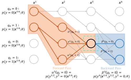
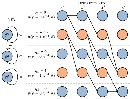
We illustrate the trellis expanded from the NFA of $W$ in MultiIns learning with $L=4$ , with the help of Figure 2 (more illustrations on other settings are shown in Section B.1), and the process of the forward-backward algorithm as shown in Figure 4. The resulting graph has 4 states at each step of the sequence, where the first two correspond to $q_{0}$ , the others to $q_{1}$ , and the trellis to the transition rules in NFA. Each path from $\mathbf{x}^{1}$ to $\mathbf{x}^{L}$ denotes an available labeling. To compute the probabilities, we define the forward score $\alpha^{j}(q=y)$ and backward score $\beta^{j}(q=y)$ for each state $q$ at step $j$ :

\begin{split}\alpha^{j}(q=y)&=\sum_{y^{\prime}\in\{y^{i-1}|\delta(q_{0},y^{1:L})\in F\}}\alpha^{i-1}(q=y^{\prime})p(y^{j}|\mathbf{x}^{1:L};\theta^{t}),\\ \hat{\beta}^{j}(q=y)&=\sum_{y^{\prime}\in\{y^{j+1}|\delta(q_{0},y^{1:L})\in F\}}\hat{\beta}^{j+1}(q=y^{\prime})p(y^{j}|\mathbf{x}^{1:L};\theta^{t}),\\ \beta^{j}(q=y)&=\frac{\hat{\beta}^{j}(q=y)}{p(y^{j}|\mathbf{x}^{1:L};\theta^{t})},\end{split}

(6)

where $\hat{\beta}^{j}(q=y)$ is used as a proxy for easier computation of $\beta^{j}(q=y)$ (Graves et al., 2006). The forward score $\alpha^{j}(q=y)$ indicates the total probability of all preceding labeling that fulfills $W$ at $j$ -th inputs with $p(y^{1:j}|\mathbf{x}^{1:L};\theta^{t})$ , and correspondingly, the backward score $\beta^{j}(q=y)$ indicates the total probability of all succeeding labeling that fulfills $W$ at $j$ -th inputs given the preceding $p(y^{j+1:L}|\mathbf{x}^{1:L},y^{1:j};\theta^{t})$ , $\forall y^{j}\in\{y^{j}|\delta(q_{0},y^{1:L})\in F\}$ . Both $\alpha^{j}(q=y)$ and $\beta^{j}(q=y)$ can be calculated recursively through the forward and backward pass on the graph, with linear complexity of $\mathcal{O}(|Q|L)$ , where $|Q|$ is the number of states on the NFA of $W$ . The joint probability at each position of the sequence thus can be calculated as:

p(y^{j},w|\mathbf{x}^{1:L};\theta^{t})=\sum_{q\in Q}\frac{\alpha^{j}(q=y^{j})\beta^{j}(q=y^{j})}{\sum_{y^{\prime}\in\mathcal{Y}}\alpha^{j}(q=y^{\prime})\beta^{j}(q=y^{\prime})}.

(7)

Moreover, the probability for supervised objective can also be easily computed as the summation of the probabilities at the accepting nodes on the graph with linear complexity:

p(w|y^{1:L},\mathbf{x}^{1:L};\theta)=\sum_{q\in F}\sum_{y^{\prime}\in\mathcal{Y}}\alpha^{L}(q=y^{\prime}).

(8)

Now, we can bring these quantities back to Equation 5 to perform training. In practice, we implement the forward-backward algorithm in log space and adopt the re-scaling strategy (McAuley and Leskovec, 2013) for numerical stability. We present the pseudo-algorithm of the forward-backward process of the common settings in Section B.2.

3.5 Extension to Multi-Class or Multi-Label Scenarios

In the analysis above, we model the NFA of $W$ only for binary classification problems. Here, we demonstrate how to extend the modeling to multi-class (multi-label) classification problems. While it is natural to extend to multiple classes, for example, for partial labels as shown in Figure 3(a), it is not straightforward to directly model the NFA of $W$ with more than two values in its symbols $\Sigma$ for aggregate observations. Considering the example with MultiIns learning, where the group of instances has two multi-class labels: at least one cat and at least one dog, the complexity of $|Q|$ in the NFA modeling will increase exponentially, thus also increasing the complexity in computing the loss functions. Instead, to deal with it, we treat each class as a separate positive class and other classes as a negative class, build an NFA on this class, and train each class as a binary classification problem with binary cross-entropy (BCE) loss. This is the common technique widely adopted in pre-training (Wightman et al., ; Touvron et al., 2022) and we demonstrate its effectiveness in Section 4.2 for weakly supervised learning.

4 Experiments

In this section, we demonstrate the universality and effectiveness of the proposed method comprehensively on various weakly supervised learning settings. We conduct the evaluation mainly on CIFAR-10 (Krizhevsky et al., 2009), CIFAR-100 (Krizhevsky et al., 2009), STL-10 (Coates et al., 2011), and ImageNet-100 (Russakovsky et al., 2015). Results on MNIST (Deng, 2012) and F-MNIST (Xiao et al., 2017) are included in the Appendix, where most of the baseline methods were evaluated. We compare our method (GLWS) on $11$ weak supervision settings of partial labels in Section 4.1, aggregate observations in Section 4.2, pairwise observations in Section 4.3, and unlabeled data in Section 4.4. Additionally, we provide more analysis and discussion in Section 4.5. We develop a codebase for implementations and experiments of all baselines and the proposed method, which will be open-sourced. Experiments are conducted three times with the average performance and standard deviation reported.

Table 1: Accuracy on partial label (PartialL) learning for instance-wise weak supervision. All results are averaged over three runs.

Dataset	CIFAR-10		CIFAR-100		STL-10		ImageNet-100
Ratio	0.50	0.70	0.10	0.20	0.10	0.30	0.01	0.05
CC	92.51 $\pm$ 0.04	89.01 $\pm$ 0.20	77.44 $\pm$ 0.32	74.60 $\pm$ 0.17	77.02 $\pm$ 0.69	73.26 $\pm$ 0.34	73.14 $\pm$ 0.94	64.67 $\pm$ 0.74
LWS	85.66 $\pm$ 0.32	80.71 $\pm$ 0.10	50.67 $\pm$ 0.33	43.51 $\pm$ 0.32	67.65 $\pm$ 0.33	58.18 $\pm$ 1.65	72.04 $\pm$ 0.77	62.13 $\pm$ 0.95
PRODEN	93.32 $\pm$ 0.23	90.26 $\pm$ 0.20	77.50 $\pm$ 0.15	74.89 $\pm$ 0.13	77.44 $\pm$ 0.26	73.19 $\pm$ 1.05	78.61 $\pm$ 0.63	77.59 $\pm$ 0.60
PiCO	93.85 $\pm$ 0.60	91.11 $\pm$ 0.70	77.80 $\pm$ 0.31	74.99 $\pm$ 0.57	77.74 $\pm$ 0.52	74.18 $\pm$ 0.41	80.93 $\pm$ 0.81	78.74 $\pm$ 1.34
RCR	94.04 $\pm$ 0.02	91.45 $\pm$ 0.10	78.03 $\pm$ 0.07	75.40 $\pm$ 0.12	78.02 $\pm$ 0.40	74.67 $\pm$ 0.56	81.52 $\pm$ 0.94	79.67 $\pm$ 1.22
GLWS	94.31 $\pm$ 0.09	92.06 $\pm$ 0.14	78.35 $\pm$ 0.11	75.82 $\pm$ 0.25	78.56 $\pm$ 0.27	74.79 $\pm$ 0.21	82.66 $\pm$ 0.54	81.09 $\pm$ 0.50

4.1 Partial Labels

Setup. Here, we evaluate the proposed method of PartialL learning for multi-class classification, where $W$ is a set of label candidates for each training instance. Following Wu et al. (2022) and Lv et al. (2020), we generate synthetic uniform partial labels for each dataset. We uniformly select labels other than the ground truth label with a specified partial ratio. For baselines, we adopt CC (Feng et al., 2020c), LWS (Wen et al., 2021), PRODEN (Lv et al., 2020), PiCO (Wang et al., 2022a), and RCR (Wu et al., 2022). We follow the hyper-parameters from Wu et al. (2022) for training all methods, with more details provided in Section C.2.1.

Results. The main results are shown in Table 1. Due to space limitations, more results are presented in Table 8 of Section C.2.2. Our method generally outperforms the baselines across different partial ratios, especially on the more practical ImageNet-100 with an improvement margin over RCR of 1.28%. The complete EM formulation serves as a generalized method of the prior arts. Moreover, our method is simple and straightforward to implement, requiring no additional loss functions like the contrastive loss in PiCO or training tricks like multiple augmentations in RCR.

4.2 Aggregate Observations

Setup. For aggregate observations, we evaluate two common settings: MultiIns learning and LProp learning. MultiIns learning considers $W$ as the indicator of at least one positive sample for a class in a bag of instances, while LProp learning views $W$ as the exact count or proportion of positive samples for a class within the bag. We form training bags with instances sampled randomly, where the bag size is Gaussian-distributed with specified parameters. Previous methods typically focus on binary classification in these settings. However, in our main paper, we extend this to multi-class classification (additional binary classification results are in Section C.3.2), with $W$ being multi-labeled. For instance, in MultiIns learning, the weak supervision could indicate that at least one positive instance for both dog and cat classes are present in a group. Baselines for our evaluation include Count Loss (Shukla et al., 2023) and UUM (Wei et al., 2023). In LProp learning, we also compare against LLP-VAT (Tsai and Lin, 2020). Details of training hyper-parameters are shown in Section C.3.1.

Table 2: Accuracy on multi-class multi-label aggregate observations of multiple instance (MultiIns) learning and label proportion (LProp) learning. All results are averaged over three runs.

Dataset	CIFAR-10		CIFAR-100		STL-10		ImageNet-100
Dist	$\mathcal{N}(10,2)$	$\mathcal{N}(20,5)$	$\mathcal{N}(5,1)$	$\mathcal{N}(10,2)$	$\mathcal{N}(5,1)$	$\mathcal{N}(10,2)$	$\mathcal{N}(3,1)$	$\mathcal{N}(5,1)$
# Bags	5,000	2,500	10,000	5,000	2,000	1,000	20,000	20,000
Multiple Instance Learning
Count Loss	86.84 $\pm$ 0.34	65.97 $\pm$ 0.94	52.04 $\pm$ 1.49	30.66 $\pm$ 0.68	73.79 $\pm$ 1.51	63.80 $\pm$ 1.66	71.48 $\pm$ 1.61	70.58 $\pm$ 1.14
UUM	13.86 $\pm$ 1.31	13.21 $\pm$ 0.52	1.27 $\pm$ 0.29	1.01 $\pm$ 0.20	18.25 $\pm$ 2.58	15.45 $\pm$ 1.66	1.33 $\pm$ 0.17	1.25 $\pm$ 0.18
GLWS	87.15 $\pm$ 0.32	71.88 $\pm$ 0.55	56.28 $\pm$ 1.16	52.29 $\pm$ 2.93	74.66 $\pm$ 1.64	64.35 $\pm$ 0.52	73.92 $\pm$ 1.38	73.08 $\pm$ 1.76
Label Proportion Learning
LLP-VAT	85.33 $\pm$ 0.44	79.70 $\pm$ 0.48	51.95 $\pm$ 2.74	52.26 $\pm$ 0.46	74.76 $\pm$ 0.08	70.76 $\pm$ 0.78	59.97 $\pm$ 3.45	68.45 $\pm$ 1.82
Count Loss	89.46 $\pm$ 0.24	84.54 $\pm$ 0.39	54.13 $\pm$ 1.43	36.21 $\pm$ 0.49	76.60 $\pm$ 0.13	73.36 $\pm$ 0.33	72.17 $\pm$ 0.47	72.21 $\pm$ 0.91
UUM	-	-	53.25 $\pm$ 1.96	-	77.26 $\pm$ 0.67	-	71.51 $\pm$ 0.94	71.14 $\pm$ 1.31
GLWS	89.77 $\pm$ 0.45	86.41 $\pm$ 0.11	58.25 $\pm$ 0.61	57.14 $\pm$ 1.71	78.27 $\pm$ 0.77	73.70 $\pm$ 0.19	73.93 $\pm$ 0.33	73.09 $\pm$ 0.84

Results. The results are presented in Table 2. Our method demonstrates a significant performance gain compared to baselines across various setups. In MultiIns learning, our method surpasses Count Loss by 1.46% on CIFAR-10, 12.93% on CIFAR-100, 0.71% on STL-10, and 2.47% on ImageNet-100, showcasing its effectiveness in more complex datasets with a larger number of classes and training group sizes. For LProp learning, it notably outperforms previous methods, with improvements of 4.50% on CIFAR-100 and 2.19% on ImageNet-100. The oversimplified modeling of UUM, while adequate for smaller bags and datasets (e.g., sizes 3 and 5, MNIST and Fashion-MNIST as shown in Table 10), makes it struggle with larger datasets and bag sizes as shown in Table 2. Furthermore, for bags with an average size greater than 5, LProp learning becomes computationally infeasible in UUM due to the factorial complexity. Compared to UUM’s factorial complexity and Count Loss’s quadratic complexity, our proposed method efficiently addresses various settings with linear complexity.

4.3 Pairwise Observations

Setup. We conduct evaluation on four common settings of pairwise observations $(\mathbf{x}^{1},\mathbf{x}^{2})$ for binary classification: PComp (Feng et al., 2021), PSim (Wei et al., 2023), SimConf (Cao et al., 2021a), and ConfDiff learning (Wang et al., 2023a). We treat a subset of classes of each dataset as the positive class, and others as the negative class. Details on the class split are shown in Section C.1. We first set a class prior, and then sample data to form the training pairs accordingly for each setting, following the baselines (Feng et al., 2021; Wei et al., 2023; Cao et al., 2021a; Wang et al., 2023a). For PComp, $W$ indicates the unlabeled pairs that $\mathbf{x}^{1}$ can only be more positive than $\mathbf{x}^{2}$ . We adopt PComp (and its variants) (Feng et al., 2021) and Rank Pruning (Northcutt et al., 2017) as baselines. For PSim, $W$ indicates whether the instances in the pair have similar labels or dissimilar labels. We use RiskSD (Shimada et al., 2021) and UUM (Wei et al., 2023) as baselines for this setting. For SimConf and ConfDiff, $W$ is the confidence score of similarity and difference between $\mathbf{x}^{1}$ and $\mathbf{x}^{2}$ , respectively. The confidence score is given by a pre-trained model, and we follow the previous method (Cao et al., 2021a; Wang et al., 2023a) to train a model on excluded data first to compute the confidence score. We additionally adopt CLIP (Radford et al., 2021; Cherti et al., 2023) with its zero-shot confidence score. Since only a non-identifiable classifiers can be learned from pairwise observations, we use clustering algorithms of Hungarian matching (Crouse, 2016) similar to Wei et al. (2023) on the predictions to evaluate. We present more training details of these settings in Section C.4.1.

Table 3: Accuracy on binary classification of pairwise comparison (PComp) and pairwise similarity (PSim) averaged over three runs.

Dataset	CIFAR-10		CIFAR-100		STL-10
Pairwise Comparison
#Pairs	20,000		20.000		5,000
Prior	0.5	0.8	0.5	0.8	0.5	0.8
PComp ABS	91.78 $\pm$ 0.10	87.37 $\pm$ 1.89	81.67 $\pm$ 0.24	66.06 $\pm$ 1.19	79.07 $\pm$ 0.40	56.45 $\pm$ 1.86
PComp ReLU	92.18 $\pm$ 0.22	90.57 $\pm$ 0.21	81.77 $\pm$ 0.59	66.57 $\pm$ 1.27	79.68 $\pm$ 0.75	67.01 $\pm$ 1.71
PComp Teacher	93.33 $\pm$ 0.38	91.35 $\pm$ 0.27	78.59 $\pm$ 0.60	67.43 $\pm$ 3.09	77.33 $\pm$ 0.14	72.88 $\pm$ 0.15
PComp Unbiased	91.71 $\pm$ 0.48	88.22 $\pm$ 0.58	67.80 $\pm$ 0.07	60.86 $\pm$ 2.19	77.46 $\pm$ 0.19	71.60 $\pm$ 0.95
Rank Pruning	93.98 $\pm$ 0.40	91.97 $\pm$ 0.27	78.90 $\pm$ 0.48	71.51 $\pm$ 0.73	77.89 $\pm$ 0.42	73.62 $\pm$ 1.38
GLWS	94.15 $\pm$ 0.10	93.28 $\pm$ 0.38	83.15 $\pm$ 0.16	80.50 $\pm$ 0.20	81.26 $\pm$ 0.54	79.24 $\pm$ 0.87
Pairwise Similarity
#Pairs	25,000		25.000		5,000
Prior	0.4	0.6	0.4	0.6	0.4	0.6
RiskSD	85.78 $\pm$ 1.70	85.61 $\pm$ 1.34	70.41 $\pm$ 0.21	64.26 $\pm$ 3.81	74.15 $\pm$ 3.27	69.35 $\pm$ 0.32
UUM	97.24 $\pm$ 0.23	97.16 $\pm$ 0.24	87.13 $\pm$ 0.40	85.19 $\pm$ 2.45	83.55 $\pm$ 0.80	83.64 $\pm$ 0.25
GLWS	97.44 $\pm$ 0.07	97.18 $\pm$ 0.22	87.25 $\pm$ 0.16	86.96 $\pm$ 0.33	84.81 $\pm$ 0.60	85.19 $\pm$ 0.26

Table 4: Accuracy on binary classification of similarity confidence (SimConf) and confidence difference (ConfDiff) over three runs.

Dataset	CIFAR-10		CIFAR-100		STL-10
#Pairs	25,000		25.000		5,000
Prior	0.4	0.4	0.4	0.4	0.4	0.4
Conf Model	WRN-28-2	CLIP ViT-B-16	ResNet-18	CLIP ViT-B-16	ResNet-18	CLIP ViT-B-16
Similarity Confidence
Sconf Abs	87.36 $\pm$ 1.22	90.16 $\pm$ 1.32	75.79 $\pm$ 0.27	69.51 $\pm$ 0.44	76.84 $\pm$ 0.75	74.44 $\pm$ 0.78
Sconf ReLU	88.56 $\pm$ 0.57	90.50 $\pm$ 0.44	74.95 $\pm$ 0.55	69.67 $\pm$ 1.51	77.40 $\pm$ 0.31	75.26 $\pm$ 0.66
Sconf NN Abs	89.04 $\pm$ 0.88	89.05 $\pm$ 2.11	74.55 $\pm$ 0.23	68.93 $\pm$ 2.00	77.55 $\pm$ 0.31	75.66 $\pm$ 0.51
Sconf Unbiased	88.72 $\pm$ 0.52	88.71 $\pm$ 0.59	72.87 $\pm$ 1.30	69.55 $\pm$ 0.31	77.76 $\pm$ 0.40	74.36 $\pm$ 0.60
GLWS	95.97 $\pm$ 0.11	97.88 $\pm$ 0.11	85.58 $\pm$ 0.88	87.94 $\pm$ 0.34	78.64 $\pm$ 0.16	79.06 $\pm$ 0.05
Confidence Difference
ConfDiff Abs	90.12 $\pm$ 4.19	88.61 $\pm$ 7.50	82.89 $\pm$ 0.32	81.45 $\pm$ 0.26	73.17 $\pm$ 2.06	77.33 $\pm$ 0.74
ConfDiff ReLU	90.36 $\pm$ 4.07	88.78 $\pm$ 7.91	83.13 $\pm$ 0.27	81.68 $\pm$ 0.46	72.39 $\pm$ 3.06	77.59 $\pm$ 0.17
ConfDiff Unbiased	90.05 $\pm$ 5.23	87.91 $\pm$ 9.03	83.65 $\pm$ 0.11	81.94 $\pm$ 0.43	72.13 $\pm$ 2.70	77.98 $\pm$ 0.08
GLWS	95.36 $\pm$ 0.19	96.14 $\pm$ 0.67	86.12 $\pm$ 0.76	83.42 $\pm$ 1.12	77.99 $\pm$ 0.75	78.49 $\pm$ 0.31

Results. We present the main results for PComp and Psim in Table 3, and for SimConf and ConfDiff in Table 4. The proposed method presents consistent and superior performance, where the improvement margin is significant especially on larger datasets. On CIFAR-100, our method improves the previous best by 10.23% on pairwise comparison and by 14.03% on similarity confidence. All the baseline methods here require the class prior in the proposed loss functions, which must be given or estimated. Ours does not require class prior and still achieves the best performance. More results of pairwise observations are in Section C.4.2.

4.4 Unlabeled Data

Setup. For unlabeled data, we consider the settings of binary classification where only the class prior is given to the unlabeled data as weak supervision: PosUlb (du Plessis et al., 2015), UlbUlb (Lu et al., 2018), and SDUlb learning (Shimada et al., 2021). We present only the results of PosUlb learning in the main paper, and other settings are shown in Section C.5.2. We similarly split the classes into either the positive subset or the negative subset as pairwise observations. For PosUlb learning, we first randomly select a specified number of positive samples as a labeled set, and treat the remaining data as an unlabeled set. For STL-10, we additionally add its split of extra data to the unlabeled set. We consider Count Loss (Shukla et al., 2023), CVIR (Garg et al., 2021), DistPU (Zhao et al., 2022), NNPU (Kiryo et al., 2017), UPU (Kiryo et al., 2017), and VarPU (Chen et al., 2020) as baselines. More details are in Section C.5.1.

Table 5: Accuracy on positive unlabeled (PosUlb) learning for binary classification. All results are averaged over three runs.

	CIFAR-10		CIFAR-100		STL-10
# Pos	500	1000	1000	2000	500	1000
Count Loss	87.76 $\pm$ 0.59	88.61 $\pm$ 0.68	70.57 $\pm$ 1.50	78.13 $\pm$ 0.19	77.11 $\pm$ 0.60	78.79 $\pm$ 0.96
CVIR	88.65 $\pm$ 2.59	93.37 $\pm$ 0.24	78.56 $\pm$ 0.22	82.94 $\pm$ 0.37	77.67 $\pm$ 1.11	81.84 $\pm$ 1.10
Dist PU	83.61 $\pm$ 4.52	82.60 $\pm$ 2.48	69.12 $\pm$ 1.39	69.83 $\pm$ 1.43	71.07 $\pm$ 1.12	70.89 $\pm$ 0.63
NN PU	87.45 $\pm$ 0.66	90.32 $\pm$ 0.50	75.49 $\pm$ 0.88	77.26 $\pm$ 0.47	74.57 $\pm$ 0.54	77.32 $\pm$ 0.95
U PU	81.38 $\pm$ 2.17	87.51 $\pm$ 0.24	68.70 $\pm$ 0.79	70.08 $\pm$ 0.98	73.37 $\pm$ 0.57	75.31 $\pm$ 0.74
Var PU	77.00 $\pm$ 2.82	84.45 $\pm$ 2.58	61.02 $\pm$ 0.22	66.02 $\pm$ 0.29	60.98 $\pm$ 0.78	62.37 $\pm$ 1.44
GLWS	91.67 $\pm$ 0.19	93.69 $\pm$ 0.28	80.30 $\pm$ 0.12	83.32 $\pm$ 0.23	79.60 $\pm$ 0.95	82.87 $\pm$ 0.83

Results. On weak supervision with unlabeled data, our method also presents superior performance, as shown in Table 5. Notably, our method outperforms the previous best by 3.02% on CIFAR-10 with 500 positive labeled data and 4.81% on CIFAR-100 with 1000 positive labeled data. Compared to Count Loss, which computes only the supervised objective in the proposed EM formulation with quadratic complexity, its performance often falls short of other baselines such as CVIR. Our method only requires linear time.

4.5 Analysis and Discussion

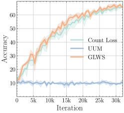
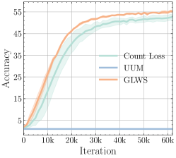
Convergence. EM algorithm might be notoriously known for difficulty in convergence and converging to local minima. We present the convergence plots, especially for aggregate observations with long sequence lengths, to show that this is not a limitation for GLWS in weakly supervised learning. As shown in Figure 5, our method converges faster to a better solution with a more stable training process (narrower error bars), compared to Count Loss (Shukla et al., 2023).

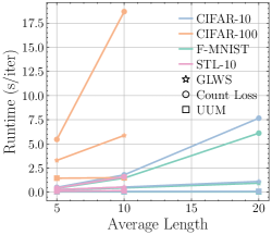
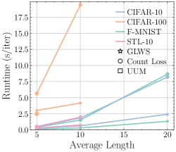
Runtime. We compare the running time explicitly in Figure 6 for aggregate observations. It is obvious that Count Loss (Shukla et al., 2023) presents (approximately) a quadratic trend in runtime as input length increases. UUM (Wei et al., 2023) shows consistent runtime for MultiIns learning with its oversimplification, leading to a practical performance gap as shown in Table 2 and Table 10. On label proportion, it is only applicable to input length of 5 because of its factorial complexity. Ours achieves the most reasonable performance and runtime trade-off with the proposed efficient algorithm.

Extension. Our framework is flexibly extensible to other settings (shown in Section C.6) and also adaptable to noisy weak supervision $\hat{W}$ with an inherent learnable noise model $P(W|\hat{W};\theta)$ in the EM, which is left for future work.

5 Conclusion

In this paper, we demonstrated a general framework for learning from arbitrary weak supervision that unifies various forms of weak supervision and can be extended to more settings flexibly, including instance partial labels, aggregate observations, pairwise observations, and unlabeled data, which addresses a significant gap in the practical applicability and scalability of weakly supervised learning methods. Experiments across various settings and practical datasets validated the superiority of the proposed method. We hope our work can inspire more research on weak supervision.

References

Radford et al. [2021] Alec Radford, Jong Wook Kim, Chris Hallacy, Aditya Ramesh, Gabriel Goh, Sandhini Agarwal, Girish Sastry, Amanda Askell, Pamela Mishkin, Jack Clark, et al. Learning transferable visual models from natural language supervision. In Proceedings of the International Conference on Machine Learning (ICML), pages 8748–8763. PMLR, 2021.
Rombach et al. [2022] Robin Rombach, Andreas Blattmann, Dominik Lorenz, Patrick Esser, and Björn Ommer. High-resolution image synthesis with latent diffusion models. In Proceedings of the IEEE/CVF conference on computer vision and pattern recognition, pages 10684–10695, 2022.
Dehghani et al. [2023] Mostafa Dehghani, Josip Djolonga, Basil Mustafa, Piotr Padlewski, Jonathan Heek, Justin Gilmer, Andreas Peter Steiner, Mathilde Caron, Robert Geirhos, Ibrahim Alabdulmohsin, et al. Scaling vision transformers to 22 billion parameters. In International Conference on Machine Learning, pages 7480–7512. PMLR, 2023.
OpenAI [2023] OpenAI. Gpt-4 technical report. 2023.
Settles et al. [2008] Burr Settles, Mark Craven, and Lewis Friedland. Active learning with real annotation costs. In Proceedings of the NIPS workshop on cost-sensitive learning, volume 1. Vancouver, CA:, 2008.
Gadre et al. [2023] Samir Yitzhak Gadre, Gabriel Ilharco, Alex Fang, Jonathan Hayase, Georgios Smyrnis, Thao Nguyen, Ryan Marten, Mitchell Wortsman, Dhruba Ghosh, Jieyu Zhang, et al. Datacomp: In search of the next generation of multimodal datasets. arXiv preprint arXiv:2304.14108, 2023.
Tommasi et al. [2017] Tatiana Tommasi, Novi Patricia, Barbara Caputo, and Tinne Tuytelaars. A deeper look at dataset bias. Domain adaptation in computer vision applications, pages 37–55, 2017.
Pagano et al. [2023] Tiago P Pagano, Rafael B Loureiro, Fernanda VN Lisboa, Rodrigo M Peixoto, Guilherme AS Guimarães, Gustavo OR Cruz, Maira M Araujo, Lucas L Santos, Marco AS Cruz, Ewerton LS Oliveira, et al. Bias and unfairness in machine learning models: a systematic review on datasets, tools, fairness metrics, and identification and mitigation methods. Big data and cognitive computing, 7(1):15, 2023.
Mireshghallah et al. [2020] Fatemehsadat Mireshghallah, Mohammadkazem Taram, Praneeth Vepakomma, Abhishek Singh, Ramesh Raskar, and Hadi Esmaeilzadeh. Privacy in deep learning: A survey. arXiv preprint arXiv:2004.12254, 2020.
Strobel and Shokri [2022] Martin Strobel and Reza Shokri. Data privacy and trustworthy machine learning. IEEE Security & Privacy, 20(5):44–49, 2022.
Zhou [2018] Zhi-Hua Zhou. A brief introduction to weakly supervised learning. National science review, 5(1):44–53, 2018.
Sugiyama et al. [2022] M. Sugiyama, H. Bao, T. Ishida, N. Lu, T. Sakai, and G. Niu. Machine Learning from Weak Supervision: An Empirical Risk Minimization Approach. MIT Press, Cambridge, Massachusetts, USA, 2022.
Luo and Orabona [2010] Jie Luo and Francesco Orabona. Learning from candidate labeling sets. Advances in Neural Information Processing Systems (NeurIPS), 2010.
Cour et al. [2011] Timothee Cour, Ben Sapp, and Ben Taskar. Learning from partial labels. The Journal of Machine Learning Research, 12:1501–1536, 2011.
Ishida et al. [2019] Takashi Ishida, Gang Niu, Aditya Menon, and Masashi Sugiyama. Complementary-label learning for arbitrary losses and models. In International Conference on Machine Learning, pages 2971–2980. PMLR, 2019.
Feng et al. [2020a] Lei Feng, Takuo Kaneko, Bo Han, Gang Niu, Bo An, and Masashi Sugiyama. Learning with multiple complementary labels. In Proceedings of the International Conference on Machine Learning (ICML), pages 3072–3081. PMLR, 2020a.
Feng et al. [2020b] Lei Feng, Jiaqi Lv, Bo Han, Miao Xu, Gang Niu, Xin Geng, Bo An, and Masashi Sugiyama. Provably consistent partial-label learning. Advances in neural information processing systems, 33:10948–10960, 2020b.
Wang et al. [2022a] Haobo Wang, Ruixuan Xiao, Yixuan Li, Lei Feng, Gang Niu, Gang Chen, and Junbo Zhao. PiCO: Contrastive label disambiguation for partial label learning. In International Conference on Learning Representations (ICLR), 2022a. URL https://openreview.net/forum?id=EhYjZy6e1gJ.
Wu et al. [2022] Dong-Dong Wu, Deng-Bao Wang, and Min-Ling Zhang. Revisiting consistency regularization for deep partial label learning. In Kamalika Chaudhuri, Stefanie Jegelka, Le Song, Csaba Szepesvari, Gang Niu, and Sivan Sabato, editors, Proceedings of the International Conference on Machine Learning (ICML), volume 162 of Proceedings of Machine Learning Research, pages 24212–24225. PMLR, 17–23 Jul 2022. URL https://proceedings.mlr.press/v162/wu22l.html.
Maron and Lozano-Pérez [1997] Oded Maron and Tomás Lozano-Pérez. A framework for multiple-instance learning. Advances in Neural Information Processing Systems (NeurIPS), 10, 1997.
Zhou [2004] Zhi-Hua Zhou. Multi-instance learning: A survey. Department of Computer Science & Technology, Nanjing University, Tech. Rep, 1, 2004.
Kück and de Freitas [2005] Hendrik Kück and Nando de Freitas. Learning about individuals from group statistics. In Proceedings of the Twenty-First Conference on Uncertainty in Artificial Intelligence, UAI’05, page 332–339, Arlington, Virginia, USA, 2005. AUAI Press. ISBN 0974903914.
Quadrianto et al. [2008] Novi Quadrianto, Alex J Smola, Tiberio S Caetano, and Quoc V Le. Estimating labels from label proportions. In Proceedings of the 25th International Conference on Machine learning, pages 776–783, 2008.
Ilse et al. [2018] Maximilian Ilse, Jakub Tomczak, and Max Welling. Attention-based deep multiple instance learning. In International Conference on Machine Learning (ICML), pages 2127–2136. PMLR, 2018.
Zhang et al. [2020] Y. Zhang, N. Charoenphakdee, Z. Wu, and M. Sugiyama. Learning from aggregate observations. pages 7993–8005, 2020.
Scott and Zhang [2020] Clayton Scott and Jianxin Zhang. Learning from label proportions: A mutual contamination framework. Advances in Neural Information Processing Systems (NeurIPS), 33:22256–22267, 2020.
Zhang et al. [2022] Jianxin Zhang, Yutong Wang, and Clay Scott. Learning from label proportions by learning with label noise. Advances in Neural Information Processing Systems, 35:26933–26942, 2022.
Bao et al. [2018] Han Bao, Gang Niu, and Masashi Sugiyama. Classification from pairwise similarity and unlabeled data. In International Conference on Machine Learning, pages 452–461. PMLR, 2018.
Bao et al. [2020] Han Bao, Takuya Shimada, Liyuan Xu, Issei Sato, and Masashi Sugiyama. Pairwise supervision can provably elicit a decision boundary. arXiv preprint arXiv:2006.06207, 2020.
Feng et al. [2021] Lei Feng, Senlin Shu, Nan Lu, Bo Han, Miao Xu, Gang Niu, Bo An, and Masashi Sugiyama. Pointwise binary classification with pairwise confidence comparisons. In International Conference on Machine Learning, pages 3252–3262. PMLR, 2021.
Cao et al. [2021a] Yuzhou Cao, Lei Feng, Yitian Xu, Bo An, Gang Niu, and Masashi Sugiyama. Learning from similarity-confidence data. In International Conference on Machine Learning, pages 1272–1282. PMLR, 2021a.
Wang et al. [2023a] Wei Wang, Lei Feng, Yuchen Jiang, Gang Niu, Min-Ling Zhang, and Masashi Sugiyama. Binary classification with confidence difference. arXiv preprint arXiv:2310.05632, 2023a.
Lu et al. [2018] Nan Lu, Gang Niu, Aditya Krishna Menon, and Masashi Sugiyama. On the minimal supervision for training any binary classifier from only unlabeled data. arXiv preprint arXiv:1808.10585, 2018.
Sohn et al. [2020] Kihyuk Sohn, David Berthelot, Nicholas Carlini, Zizhao Zhang, Han Zhang, Colin A Raffel, Ekin Dogus Cubuk, Alexey Kurakin, and Chun-Liang Li. Fixmatch: Simplifying semi-supervised learning with consistency and confidence. Advances in Neural Information Processing Systems (NeurIPS), 33, 2020.
Shimada et al. [2021] Takuya Shimada, Han Bao, Issei Sato, and Masashi Sugiyama. Classification from pairwise similarities/dissimilarities and unlabeled data via empirical risk minimization. Neural Computation, 33(5):1234–1268, 2021.
Wang et al. [2022b] Yidong Wang, Hao Chen, Yue Fan, Wang Sun, Ran Tao, Wenxin Hou, Renjie Wang, Linyi Yang, Zhi Zhou, Lan-Zhe Guo, Heli Qi, Zhen Wu, Yu-Feng Li, Satoshi Nakamura, Wei Ye, Marios Savvides, Bhiksha Raj, Takahiro Shinozaki, Bernt Schiele, Jindong Wang, Xing Xie, and Yue Zhang. Usb: A unified semi-supervised learning benchmark. In Advances in Neural Information Processing Systems (NeurIPS), 2022b.
Tang et al. [2023] Yuting Tang, Nan Lu, Tianyi Zhang, and Masashi Sugiyama. Multi-class classification from multiple unlabeled datasets with partial risk regularization. In Asian Conference on Machine Learning, pages 990–1005. PMLR, 2023.
Van Rooyen and Williamson [2018] Brendan Van Rooyen and Robert C Williamson. A theory of learning with corrupted labels. Journal of Machine Learning Research, 18(228):1–50, 2018.
Chiang and Sugiyama [2023] Chao-Kai Chiang and Masashi Sugiyama. Unified risk analysis for weakly supervised learning. arXiv preprint arXiv:2309.08216, 2023.
Shukla et al. [2023] Vinay Shukla, Zhe Zeng, Kareem Ahmed, and Guy Van den Broeck. A unified approach to count-based weakly-supervised learning. In ICML 2023 Workshop on Differentiable Almost Everything: Differentiable Relaxations, Algorithms, Operators, and Simulators, jul 2023. URL http://starai.cs.ucla.edu/papers/ShuklaDAE23.pdf.
Wei et al. [2023] Zixi Wei, Lei Feng, Bo Han, Tongliang Liu, Gang Niu, Xiaofeng Zhu, and Heng Tao Shen. A universal unbiased method for classification from aggregate observations. In Andreas Krause, Emma Brunskill, Kyunghyun Cho, Barbara Engelhardt, Sivan Sabato, and Jonathan Scarlett, editors, Proceedings of the 40th International Conference on Machine Learning, volume 202 of Proceedings of Machine Learning Research, pages 36804–36820. PMLR, 23–29 Jul 2023. URL https://proceedings.mlr.press/v202/wei23a.html.
Yan et al. [2018] Yongluan Yan, Xinggang Wang, Xiaojie Guo, Jiemin Fang, Wenyu Liu, and Junzhou Huang. Deep multi-instance learning with dynamic pooling. In Asian Conference on Machine Learning, pages 662–677. PMLR, 2018.
Yang et al. [2022] Mei Yang, Yu-Xuan Zhang, Mao Ye, and Fan Min. Attention-to-embedding framework for multi-instance learning. In Pacific-Asia Conference on Knowledge Discovery and Data Mining, pages 109–121. Springer, 2022.
Cui et al. [2020] Zhenghang Cui, Nontawat Charoenphakdee, Issei Sato, and Masashi Sugiyama. Classification from triplet comparison data. Neural Computation, 32(3):659–681, 2020.
Dempster et al. [1977] Arthur P Dempster, Nan M Laird, and Donald B Rubin. Maximum likelihood from incomplete data via the em algorithm. Journal of the royal statistical society: series B (methodological), 39(1):1–22, 1977.
Rabiner [1989] Lawrence R Rabiner. A tutorial on hidden markov models and selected applications in speech recognition. Proceedings of the IEEE, 77(2):257–286, 1989.
Graves et al. [2006] Alex Graves, Santiago Fernández, Faustino Gomez, and Jürgen Schmidhuber. Connectionist temporal classification: labelling unsegmented sequence data with recurrent neural networks. In Proceedings of the International Conference on Machine Learning (ICML), pages 369–376, 2006.
Rabin and Scott [1959] Michael O Rabin and Dana Scott. Finite automata and their decision problems. IBM journal of research and development, 3(2):114–125, 1959.
Denœux [2011] Thierry Denœux. Maximum likelihood estimation from fuzzy data using the em algorithm. Fuzzy sets and systems, 183(1):72–91, 2011.
Quost and Denoeux [2016] Benjamin Quost and Thierry Denoeux. Clustering and classification of fuzzy data using the fuzzy em algorithm. Fuzzy Sets and Systems, 286:134–156, 2016.
Feng et al. [2020c] Lei Feng, Jiaqi Lv, Bo Han, Miao Xu, Gang Niu, Xin Geng, Bo An, and Masashi Sugiyama. Provably consistent partial-label learning. ArXiv, abs/2007.08929, 2020c.
Wang et al. [2019] Dengbao Wang, Min-Ling Zhang, and Li Li. Adaptive graph guided disambiguation for partial label learning. IEEE Transactions on Pattern Analysis and Machine Intelligence, 44:8796–8811, 2019.
Wen et al. [2021] Hongwei Wen, Jingyi Cui, Hanyuan Hang, Jiabin Liu, Yisen Wang, and Zhouchen Lin. Leveraged weighted loss for partial label learning. In Proceedings of the International Conference on Machine Learning (ICML), pages 11091–11100. PMLR, 2021.
Xie et al. [2020] Qizhe Xie, Zihang Dai, Eduard Hovy, Thang Luong, and Quoc Le. Unsupervised data augmentation for consistency training. Advances in Neural Information Processing Systems (NeurIPS), 33, 2020.
Zhang et al. [2021] Bowen Zhang, Yidong Wang, Wenxin Hou, Hao Wu, Jindong Wang, Manabu Okumura, and Takahiro Shinozaki. Flexmatch: Boosting semi-supervised learning with curriculum pseudo labeling. Advances in Neural Information Processing Systems (NeurIPS), 34, 2021.
Wang et al. [2023b] Yidong Wang, Hao Chen, Qiang Heng, Wenxin Hou, Yue Fan, , Zhen Wu, Jindong Wang, Marios Savvides, Takahiro Shinozaki, Bhiksha Raj, Bernt Schiele, and Xing Xie. Freematch: Self-adaptive thresholding for semi-supervised learning. In International Conference on Learning Representations (ICLR), 2023b.
Chen et al. [2023] Hao Chen, Ran Tao, Yue Fan, Yidong Wang, Jindong Wang, Bernt Schiele, Xing Xie, Bhiksha Raj, and Marios Savvides. Softmatch: Addressing the quantity-quality trade-off in semi-supervised learning. In International Conference on Learning Representations (ICLR), 2023.
du Plessis et al. [2015] Marthinus du Plessis, Gang Niu, and Masashi Sugiyama. Convex formulation for learning from positive and unlabeled data. In International conference on machine learning, pages 1386–1394. PMLR, 2015.
Hammoudeh and Lowd [2020] Zayd Hammoudeh and Daniel Lowd. Learning from positive and unlabeled data with arbitrary positive shift. Advances in Neural Information Processing Systems, 33:13088–13099, 2020.
Chen et al. [2020] Hui Chen, Fangqing Liu, Yin Wang, Liyue Zhao, and Hao Wu. A variational approach for learning from positive and unlabeled data. Advances in Neural Information Processing Systems, 33:14844–14854, 2020.
Garg et al. [2021] Saurabh Garg, Yifan Wu, Alex Smola, Sivaraman Balakrishnan, and Zachary C. Lipton. Mixture proportion estimation and pu learning: A modern approach, 2021.
Kiryo et al. [2017] Ryuichi Kiryo, Gang Niu, Marthinus C Du Plessis, and Masashi Sugiyama. Positive-unlabeled learning with non-negative risk estimator. Advances in neural information processing systems, 30, 2017.
Zhao et al. [2022] Yunrui Zhao, Qianqian Xu, Yangbangyan Jiang, Peisong Wen, and Qingming Huang. Dist-pu: Positive-unlabeled learning from a label distribution perspective. In Proceedings of the IEEE/CVF Conference on Computer Vision and Pattern Recognition, pages 14461–14470, 2022.
Hsu et al. [2019] Yen-Chang Hsu, Zhaoyang Lv, Joel Schlosser, Phillip Odom, and Zsolt Kira. Multi-class classification without multi-class labels. arXiv preprint arXiv:1901.00544, 2019.
Yu et al. [2014] Felix X Yu, Krzysztof Choromanski, Sanjiv Kumar, Tony Jebara, and Shih-Fu Chang. On learning from label proportions. arXiv preprint arXiv:1402.5902, 2014.
McAuley and Leskovec [2013] Julian McAuley and Jure Leskovec. Hidden factors and hidden topics: understanding rating dimensions with review text. In Proceedings of the 7th ACM conference on Recommender systems, pages 165–172, 2013.
[67] R Wightman, H Touvron, and H Jégou. Resnet strikes back: An improved training procedure in timm. arxiv 2021. arXiv preprint arXiv:2110.00476.
Touvron et al. [2022] Hugo Touvron, Matthieu Cord, and Hervé Jégou. Deit iii: Revenge of the vit. In European Conference on Computer Vision, pages 516–533. Springer, 2022.
Krizhevsky et al. [2009] Alex Krizhevsky et al. Learning multiple layers of features from tiny images. 2009.
Coates et al. [2011] Adam Coates, Andrew Ng, and Honglak Lee. An analysis of single-layer networks in unsupervised feature learning. In Proceedings of the fourteenth international conference on artificial intelligence and statistics, pages 215–223. JMLR Workshop and Conference Proceedings, 2011.
Russakovsky et al. [2015] Olga Russakovsky, Jia Deng, Hao Su, Jonathan Krause, Sanjeev Satheesh, Sean Ma, Zhiheng Huang, Andrej Karpathy, Aditya Khosla, Michael Bernstein, et al. Imagenet large scale visual recognition challenge. International journal of computer vision, 115:211–252, 2015.
Deng [2012] Li Deng. The mnist database of handwritten digit images for machine learning research. IEEE Signal Processing Magazine, 29(6):141–142, 2012.
Xiao et al. [2017] Han Xiao, Kashif Rasul, and Roland Vollgraf. Fashion-mnist: a novel image dataset for benchmarking machine learning algorithms, 2017.
Lv et al. [2020] Jiaqi Lv, Miao Xu, Lei Feng, Gang Niu, Xin Geng, and Masashi Sugiyama. Progressive identification of true labels for partial-label learning. In Proceedings of the International Conference on Machine Learning (ICML), pages 6500–6510. PMLR, 2020.
Tsai and Lin [2020] Kuen-Han Tsai and Hsuan-Tien Lin. Learning from label proportions with consistency regularization. In Asian Conference on Machine Learning, pages 513–528. PMLR, 2020.
Northcutt et al. [2017] Curtis G Northcutt, Tailin Wu, and Isaac L Chuang. Learning with confident examples: Rank pruning for robust classification with noisy labels. arXiv preprint arXiv:1705.01936, 2017.
Cherti et al. [2023] Mehdi Cherti, Romain Beaumont, Ross Wightman, Mitchell Wortsman, Gabriel Ilharco, Cade Gordon, Christoph Schuhmann, Ludwig Schmidt, and Jenia Jitsev. Reproducible scaling laws for contrastive language-image learning. In Proceedings of the IEEE/CVF Conference on Computer Vision and Pattern Recognition, pages 2818–2829, 2023.
Crouse [2016] David F Crouse. On implementing 2d rectangular assignment algorithms. IEEE Transactions on Aerospace and Electronic Systems, 52(4):1679–1696, 2016.
LeCun et al. [1998] Yann LeCun, Léon Bottou, Yoshua Bengio, and Patrick Haffner. Gradient-based learning applied to document recognition. Proceedings of the IEEE, 86(11):2278–2324, 1998.
Zagoruyko and Komodakis [2016] Sergey Zagoruyko and Nikos Komodakis. Wide residual networks. In British Machine Vision Conference (BMVC). British Machine Vision Association, 2016.
He et al. [2016] Kaiming He, Xiangyu Zhang, Shaoqing Ren, and Jian Sun. Deep residual learning for image recognition. In Proceedings of the IEEE/CVF Conference on Computer Vision and Pattern Recognition (CVPR), pages 770–778, 2016.
Loshchilov and Hutter [2016] Ilya Loshchilov and Frank Hutter. Sgdr: Stochastic gradient descent with warm restarts. International Conference on Learning Representations (ICLR), 2016.
Kingma and Ba [2014] Diederik P Kingma and Jimmy Ba. Adam: A method for stochastic optimization. arXiv preprint arXiv:1412.6980, 2014.
Ishida et al. [2018] Takashi Ishida, Gang Niu, and Masashi Sugiyama. Binary classification from positive-confidence data. Advances in neural information processing systems, 31, 2018.
Cao et al. [2021b] Yuzhou Cao, Lei Feng, Senlin Shu, Yitian Xu, Bo An, Gang Niu, and Masashi Sugiyama. Multi-class classification from single-class data with confidences. arXiv preprint arXiv:2106.08864, 2021b.
Ishida et al. [2022] Takashi Ishida, Ikko Yamane, Nontawat Charoenphakdee, Gang Niu, and Masashi Sugiyama. Is the performance of my deep network too good to be true? a direct approach to estimating the bayes error in binary classification. arXiv preprint arXiv:2202.00395, 2022.

Appendix A Proofs

A.1 Derivation of Equation 4

Evidence lower bound (ELBO), or equivalently variational lower bound [Dempster et al., 1977], is the core quantity in EM. We provide the detailed derivation for Equation 4 here. To model $\log P(X,W;\theta)$ :

\begin{split}\log P(X,W;\theta)&=\log\sum_{Y}P(X,W,Y;\theta)\\ &=\log Q(Y)\frac{P(X,W,Y;\theta)}{Q(Y)}\\ &=\log\mathbb{E}_{Q(Y)}[\frac{P(X,W,Y;\theta)}{Q(Y)}]\\ &\geq\mathbb{E}_{Q(Y)}[\log\frac{P(X,W,Y;\theta)}{Q(Y)}]\quad\text{{Jensen\textquoteright s inequality}}\\ &=\mathbb{E}_{Q(Y)}[\log P(X,W,Y;\theta)]-\mathbb{E}_{Q(Y)}[\log Q(Y)]\\ &=ELBO(\theta,Q(Y)),\\ \end{split}

(9)

where the first term in ELBO is the lower bound and the second term is the entropy over $Q(Y)$ that is independent of $\theta$ . Given the ELBO, we also have:

\begin{split}ELBO(\theta,Q(Y))&=\mathbb{E}_{Q(Y)}[\log\frac{P(X,W,Y;\theta)}{Q(Y)}]\\ &=\mathbb{E}_{Q(Y)}[\log\frac{P(X,W,Y;\theta)P(Y|X,W;\theta)}{Q(Y)P(Y|X,W;\theta)}]\\ &=\mathbb{E}_{Q(Y)}[\log\frac{P(Y|X,W;\theta)P(X,W;\theta)P(Y|X,W;\theta)}{Q(Y)P(Y|X,W;\theta)}]\\ &=\mathbb{E}_{Q(Y)}[\log P(X,W;\theta)\frac{P(Y|X,W;\theta)}{Q(Y)}]\\ &=\mathbb{E}_{Q(Y)}[\log P(X,W;\theta)]-\mathbb{E}_{Q(Y)}[\frac{Q(Y)}{P(Y|X,W;\theta)}]\\ &=\log P(X,W;\theta)-\mathrm{KL}(Q(Y)||P(Y|X,W;\theta)).\end{split}

(10)

Thus we can see that maximizing the ELBO is equivalent to maximizing $\log P(X,W;\theta)$ when $P(Y|X,W;\theta)$ is close to $Q(Y)$ , i.e., the Kullback-Leibier divergence $\mathrm{KL}(Q(Y)||P(Y|X,W;\theta))$ is approaching to 0. Thus we take $Q(Y)=P(Y|X,Y;\theta^{t})$ with current estimation $\theta^{t}$ from the model, and obtain Equation 4.

A.2 Proof of Equation 5

Proof.

Applying the maximum log-likelihood estimation to the weak supervision dataset $\mathcal{D}=\{(\mathbf{x}_{i}^{1:L},w_{i})\}_{i\in[N]}$ , where $w\in W$ is the weak supervision for each sequence input $\mathbf{x}^{1:L}$ with $L\geq 1$ . When $L=1$ , $\mathbf{x}$ represents an individual training instance, otherwise it represents a group of sequence as discussed in the main paper. For simplicity, we consider $L$ as a fixed value for $\mathcal{L}$ here, but in practice it can denote variable length. We have 3.1 that the predictions and precise labels in the sequence are conditionally independent given whole input sequence.

\begin{split}&\operatorname*{arg\,max}_{\theta}\mathbb{E}_{Y|X,W;\theta^{t}}[\log P(X,W,Y;\theta)]\\ =&\operatorname*{arg\,max}_{\theta}\mathbb{E}_{Y|X,W;\theta^{t}}[\log P(W|Y,X;\theta)P(Y|X;\theta)P(X;\theta)]\\ =&\operatorname*{arg\,max}_{\theta}\mathbb{E}_{Y|X,W;\theta^{t}}[\log P(Y|X;\theta)]+\mathbb{E}_{Y|X,W;\theta^{t}}[\log P(W|Y,X;\theta)]\quad\text{{ $P(X)$ is independent of $\theta$}}\\ =&\operatorname*{arg\,max}_{\theta}\mathbb{E}_{Y|X,W;\theta^{t}}[\log P(Y|X;\theta)]+\log P(W|Y,X;\theta)\quad\text{{ $P(W|Y,X;\theta)$ is fixed for any $P(Y|X,W;\theta^{t})$ }}\end{split}

(11)

The derived objective $\mathcal{L}_{\mathrm{Weak}}$ on the dataset $\mathcal{D}$ from the EM formulation thus have two terms, where the first unsupervised term $\mathcal{L}_{\mathrm{U}}$ corresponds to:

\begin{split}\mathcal{L}_{\mathrm{U}}&=\sum_{i=1}^{N}\mathbb{E}_{y_{i}^{1:L}|\mathbf{x}_{i}^{1:L},w_{i};\theta^{t}}[\log p(y_{i}^{1:L}|\mathbf{x}_{i}^{1:L};\theta)]\\ &=\sum_{i=1}^{N}p(y_{i}^{1:L}|\mathbf{x}_{i}^{1:L},w_{i};\theta^{t})\log\prod_{j=1}^{L}p(y_{i}^{j}|\mathbf{x}_{i}^{j};\theta)\quad\text{{Instance-level model}}\\ &=\sum_{i=1}^{N}\sum_{j=1}^{L}p(y_{i}^{j}|\mathbf{x}_{i}^{1:L},w_{i};\theta^{t})\log p(y_{i}^{j}|\mathbf{x}_{i}^{j};\theta)\quad\text{{Conditional independence in \lx@cref{creftype~refnum}{assump}}},\end{split}

(12)

and the supervised term $\mathcal{L}_{\mathrm{S}}$ as:

\mathcal{L}_{S}=\sum_{i=1}^{N}\log p(w_{i}|y_{i}^{1:L},\mathbf{x}_{i}^{1:L};\theta)

(13)

∎

Appendix B Method

B.1 Illustration of Possible Labelings as Trellis of Common Weak Supervision Settings

Here, we present more illustration of the expanded trellis from the NFA in Figure 3. The demonstration of weak supervision is over a group of 4 instances for LProp and 2 instances for pairwise observations.

The trellis of LProp with exact two positive samples is shown in Figure 7. Note that for LProp, the number of states in its NFA depends on the exact count from the weak supervision as discussed in the main paper. The unlabeled data with class prior information can also be represented as expected label count and uses the trellis representation of LProp.

We also present the illustration of PComp, PSim, and PDsim in Figure 8, Figure 9(a), and Figure 9(b) respectively. Although we use 3 states in their NFA, we instead directly use 4 states in the expanded trellis to represent all the labelings for pairwise observations, i.e., $\{(0,0),(1,1),(0,1),(1,0)\}$ . Despite the notation difference, they represent the same weak supervision. SimConf and ConfDiff can also be represented similarly by weighting the path with confidence score and similarity score.

For totally unlabeled data, every symbol in $\mathcal{Y}$ can be allowed for transition, thus its trellis degenerate to the prediction probability of each instance.

B.2 Pseudo-algorithm of the Forward-Backward Algorithm of Common Weak Supervision Settings

We present the pseudo-algorithm of performing the forward-backward algorithms on common weak supervision settings we evaluated. The pseudo-algorithm also corresponds to description of the trellis expanded from the NFA. Note that the only difference for each weak supervision setting is the NFA modeling. Once having the NFA modeling of weak supervision, the finite states and the transition between states are determined, and thus the forward-backward algorithm can be performed accordingly. We perform the forward-backward algorithm in log-space for numerical stability. Moreover, we use the log-sum-exp trick for computing the addition in log-space. For illustration simplicity, we present the pseudo-algorithm on single instance/group inputs and binary predictions, but in practice we implement the forward-backward pass at batch of instances/groups inputs and multi-class predictions. Here we illustrate the pseudo-algorithm for MultiIns in Algorithm 1, LProp in Algorithm 2, PComp in Algorithm 3, respectively. Other settings should either be similar or simple to solve.

Algorithm 1 Forward-Backward Algorithm for multiple instance (MultiIns) Learning

0: Predicted probability in log-space as

log\_probs

from

\mathbf{x}^{1:L}

w

with 0 for no positive and 1 for at least one positive in the bag, bag length as

L

1: Number of states as

Q\leftarrow 4

2: Initialize

\alpha\in\mathbb{R}^{2Q\times L}

with

-1e12

for forward pass.

\alpha[0,0],\alpha[1,0]\leftarrow log\_probs[0,0],log\_probs[0,1]

4: for

i=1

L

5: if

i<L-1

then

6: Update

\alpha[0,i]=\alpha[0,i-1]+log\_probs[i,0]

7: else

8: Update

\alpha[0,i]=-1e12

9: end if

10: if

i\geq 2

then

11: Update

\alpha[2,i]=\alpha[1,i-1]+\alpha[2,i-1]+\alpha[3,i-1]+log\_probs[i,0]

12: Update

\alpha[3,i]=\alpha[1,i-1]+\alpha[2,i-1]+\alpha[3,i-1]+log\_probs[i,1]

13: else

14: Update

\alpha[2,i]=\alpha[1,i-1]+log\_probs[i,0]

15: Update

\alpha[3,i]=\alpha[1,i-1]+log\_probs[i,1]

16: end if

17: end for

18: Compute forward probability

p(w|\mathbf{x}^{1:L},y^{1:L};\theta)

from

\exp(\alpha)

sup\_preds

19: if w = 0 then

20:

em\_targets=ones\_like(log\_probs)

21: Return

sup\_preds

em\_targets

22: end if

23: Initialize

\beta\in\mathbb{R}^{2Q\times L}

with

-1e12

for backward pass.

24:

\beta[1,L-1],\beta[2,L-1],\beta[3,L-1]\leftarrow log\_probs[L-1,1],log\_probs[L-1,0],log\_probs[L-1,1]

25: for

i=L-2

down to

0

26:

\beta[0,i]=\beta[0,i+1]+\beta[1,i+1]+log\_probs[i,0]

27:

\beta[1,i]=\beta[2,i+1]+\beta[3,i+1]+log\_probs[i,1]

28: if

i>0

then

29:

\beta[2,i]=\beta[2,i+1]+\beta[3,i+1]+log\_probs[i,0]

30:

\beta[3,i]=\beta[2,i+1]+\beta[3,i+1]+log\_probs[i,1]

31: end if

32: end for

33: Adjust

\beta

based on

log\_probs

34:

\gamma=\alpha+\beta

35:

\gamma=\exp(\gamma.transpose(0,1))

36: Compute joint probability

p(y^{j}|\mathbf{x}^{1:L},w;\theta)

em\_targets

37: Return

sup\_preds

em\_targets

Algorithm 2 Forward-Backward Algorithm for label proportion (LProp) Learning

0: Predicted probability in log-space as

log\_probs

\mathbf{x}^{1:L}

w

indicates the count of positive instance.

1: Number of states

Q\leftarrow 2\times w+1

2: Initialize

\alpha\in\mathbb{R}^{Q\times L}

with

-1e12

for forward pass.

\alpha[0,0]\leftarrow log\_probs[0,0]

4: if

count>0

then

\alpha[1,0]\leftarrow log\_probs[0,1]

6: end if

7: for

i=1

L

8: Update

\alpha[0,i]=\alpha[0,i-1]+log\_probs[i,0]

9: if

count>0

then

10: Update

\alpha[1,i]=\alpha[0,i-1]+log\_probs[i,1]

11: end if

12: for

j=2

Q

13: if

i<w-(Q-j)//2

then

14: Continue to next iteration of

j

15: end if

16: if j % 2 = 0 then

17: Update

\alpha[j,i]=\alpha[j,i-1]+\alpha[j-1,i-1]+log\_probs[i,0]

18: else

19: Update

\alpha[j,i]=\alpha[j-1,i-1]+\alpha[j-2,i-1]+log\_probs[i,1]

20: end if

21: end for

22: end for

23: Compute forward probability

sup\_preds

from

\exp(\alpha)

24: Adjust

\alpha

based on

w

and

Q

to avoid underflow.

25: Initialize

\beta\in\mathbb{R}^{Q\times L}

with

-1e12

for backward pass.

26: Set initial values of

\beta[-1,-1]

and

\beta[-2,-1]

based on

w

27: for

i=b-2

down to

0

28: if

i\geq w

then

29:

\beta[-1,i]=\beta[-1,i+1]+log\_probs[i,0]

30: end if

31: if

i\geq w\&w>0

then

32:

\beta[-2,i]=\beta[-1,i+1]+log\_probs[i,0]

33: end if

34: for

j=0

k-2

35: if

i<count-(k-j)//2

then

36: Continue to next iteration of

j

37: end if

38: if j % 2 = 0 then

39: Update

\beta[j,i]=\beta[j,i+1]+\beta[j+1,i+1]+log\_probs[i,0]

40: else

41: Update

\beta[j,i]=\beta[j+1,i+1]+\beta[j+2,i+1]+log\_probs[i,1]

42: end if

43: end for

44: end for

45: Adjust

\beta

based on

log\_probs

46:

\beta=\exp(\beta)

47:

\gamma=\alpha+\beta

48:

\gamma=\exp(\gamma.transpose(0,1))

49: Compute joint probability

p(y^{j}|\mathbf{x}^{1:L},w;\theta)

em\_targets

50: Return

sup\_preds

em\_targets

Algorithm 3 Forward-Backward Algorithm for pairwise comparison (PComp) Learning

0: Predicted probability in log-space as

log\_probs

\mathbf{x}^{1:L}

1: Number of states

Q\leftarrow 4

2: Initialize

\log\_alpha\in\mathbb{R}^{4\times 2}

with

-1e12

for the forward pass.

\alpha[0,0]=log\_probs[0,0]

\alpha[1,0]=log\_probs[0,1]

\alpha[3,0]=log\_probs[0,1]

\alpha[0,1]=\alpha[0,0]+log\_probs[1,0]

\alpha[1,1]=\alpha[1,0]+log\_probs[1,1]

\alpha[2,1]=\alpha[3,0]+log\_probs[1,0]

9: Compute forward probability from

\exp(\alpha)

10: Initialize

\log\_beta\in\mathbb{R}^{4\times 2}

with

-1e12

for the backward pass.

11:

\beta[0,1]=log\_probs[1,0]

12:

\beta[1,1]=log\_probs[1,1]

13:

\beta[2,1]=log\_probs[1,0]

14:

\beta[0,0]=\beta[0,1]+log\_probs[0,0]

15:

\beta[1,0]=\beta[1,1]+log\_probs[0,1]

16:

\beta[3,0]=\beta[1,2]+log\_probs[0,1]

17: Adjust

\beta

based on repeated

log\_probs

18:

\gamma=\alpha+\beta

19:

\gamma=\exp(\gamma.transpose(0,1))

20: Compute the EM targets

em\_targets

from

\gamma

21: Return

em\_targets

sup\_preds

Appendix C Experiments

In this section, we provide more details on the training setup and hyper-parameters for our evaluations. We also present the details on datasets and class split of the datasets. More results of other weak supervision settings can be found in Section C.6.

C.1 Datasets and Classes Splits

Table 6: Dataset details

Dataset	# Classes	# Training	# Validation	# Unlabeled
MNIST	10	60,000	10,000	-
F-MNIST	10	60,000	10,000	-
CIFAR-10	10	50,000	10,000	-
CIFAR-100	100	50,000	10,000	-
STL-10	10	5,000	8,000	100,000
ImageNet-100	100	130,000	5,000	-

The datasets details are shown in Table 6.

For some weak supervision settings, such as pairwise observations, positive unlabeled, and unlabeled unlabeled learning, we split the classes of each dataset into binary as follows.

MNIST. For multiple instance learning and label proportion learning, we set digit 9 as positive class, and others as negative class for binary classification. For other settings, we set digits 0-4 as positive class, and others as negative class.

F-MNIST. Similarly, for multiple instance learning and label proportion learning, we set the 9-th class as positive class. For other settings, we set the classes related to tops as positive class, i.e., $\{5,7,9\}$ .

CIFAR-10 and STL-10. For multiple instance learning and label proportion learning, we set bird, i.e., class 3, as positive class. For other settings, we set transportation related classes as positive class, i.e., airplane, automobile, ship, truck.

CIFAR-100. Binary classification on CIFAR-100 is not conduced on multiple instance learning and label proportion learning. For other settings, we select the 40 animal related classes from 100 total classes as positive class.

C.2 Partial Labels

Here we provide more training details and results of partial label learning.

C.2.1 Setup

We follow RCR [Wu et al., 2022] for experiments of partial label learning. More specifically, we generate synthetic uniform partial label datasets, where we uniformly select each incorrect label for each instance into a candidate label set with partial ratio as probability. We adopt same training hyper-parameters for the baseline methods and GLWS for fair comparison. A summarize of training parameters is shown in Table 7.

Table 7: Hyper-parameters for partial label (PartialL) learning used in experiments.

Hyper-parameter	MNIST & F-MNIST	CIFAR-10	CIFAR-100	STL-10	ImageNet-100
Image Size	28	32	32	96	224
Model	LeNet-5	WRN-34-10	WRN-34-10	ResNet-18	ResNet-34
Batch Size	64	64	64	64	32
Optimizer	SGD	SGD	SGD	AdamW	AdamW
Learning Rate	0.1	0.1	0.1	0.001	0.001
Weight Decay	1e-4	1e-4	1e-4	1e-4	1e-4
LR Scheduler	MultiStep	MultiStep	MultiStep	Cosine	Cosine
Training Epochs	200	200	200	200	200

For MNIST and F-MNIST, we use LeNet-5 [LeCun et al., 1998]. We adopt WideResNet-34-10 variant [Zagoruyko and Komodakis, 2016] for CIFAR-10 and CIFAR-100, ResNet-18 [He et al., 2016] for STL-10, and ResNet-34 for ImageNet-100. For optimizer, we use SGD [Loshchilov and Hutter, 2016] for MNIST, F-MNIST, CIFAR-10, CIFAR-100, and AdamW [Kingma and Ba, 2014] for STL-10 and ImageNet-100.

C.2.2 Results

We present more results on partial label learning in Table 8, where our method in general achieves the best performance.

Table 8: Accuracy on partial label (PartialL) learning. All results are averaged over three runs. This table is complementary to Table 1.

Dataset

MNIST

F-MNIST

CIFAR-10

CIFAR-100

STL-10

ImageNet-100

Partial Ratio

0.10

0.30

0.50

0.70

0.10

0.300

0.50

0.70

0.10

0.30

0.50

0.70

0.01

0.05

0.10

0.20

0.10

0.30

0.01

0.05

99.25

\pm

0.02

99.18

\pm

0.05

99.08

\pm

0.03

98.93

\pm

0.05

91.44

\pm

0.16

91.10

\pm

0.07

90.45

\pm

0.09

89.55

\pm

0.28

95.25

\pm

0.03

94.13

\pm

0.09

92.51

\pm

0.04

89.01

\pm

0.20

79.68

\pm

0.14

78.73

\pm

0.24

77.44

\pm

0.32

74.60

\pm

0.17

77.02

\pm

0.69

73.26

\pm

0.34

73.14

\pm

0.94

64.67

\pm

0.74

LWS

98.23

\pm

0.02

98.04

\pm

0.12

97.95

\pm

0.11

96.96

\pm

0.10

88.17

\pm

0.11

88.10

\pm

0.05

87.59

\pm

0.18

86.60

\pm

0.13

91.42

\pm

0.03

88.76

\pm

0.45

85.66

\pm

0.32

80.71

\pm

0.10

69.46

\pm

0.28

55.49

\pm

0.67

50.67

\pm

0.33

43.51

\pm

0.32

67.65

\pm

0.33

58.18

\pm

1.65

72.04

\pm

0.77

62.13

\pm

0.95

PRODEN

99.12

\pm

0.52

98.89

\pm

0.52

98.27

\pm

0.68

97.77

\pm

0.82

90.95

\pm

0.63

91.96

\pm

0.70

90.40

\pm

0.58

89.20

\pm

0.45

95.25

\pm

0.45

95.68

\pm

0.40

93.85

\pm

0.60

91.11

\pm

0.70

79.06

\pm

0.24

79.17

\pm

0.36

77.80

\pm

0.31

74.99

\pm

0.57

77.74

\pm

0.52

74.18

\pm

0.41

78.61

\pm

0.63

77.59

\pm

0.60

PiCO

99.22

\pm

0.01

99.20

\pm

0.01

99.10

\pm

0.02

98.96

\pm

0.09

90.30

\pm

1.44

91.41

\pm

0.05

90.42

\pm

0.14

89.73

\pm

0.21

95.37

\pm

0.12

95.14

\pm

0.16

93.32

\pm

0.23

90.26

\pm

0.20

79.49

\pm

0.13

78.71

\pm

0.18

77.50

\pm

0.15

74.89

\pm

0.13

77.44

\pm

0.26

73.19

\pm

1.05

80.93

\pm

0.81

78.74

\pm

1.34

RCR

99.25

\pm

0.04

99.21

\pm

0.04

99.11

\pm

0.03

99.01

\pm

0.05

91.26

\pm

0.17

91.26

\pm

0.08

90.82

\pm

0.12

90.06

\pm

0.03

95.57

\pm

0.19

94.65

\pm

0.05

94.04

\pm

0.02

91.45

\pm

0.10

79.89

\pm

0.23

78.93

\pm

0.30

78.03

\pm

0.07

75.40

\pm

0.12

78.02

\pm

0.40

74.67

\pm

0.56

81.52

\pm

0.94

79.67

\pm

1.22

GLWS

99.25

\pm

0.01

99.28

\pm

0.05

99.12

\pm

0.02

99.14

\pm

0.04

91.42

\pm

0.22

91.28

\pm

0.09

90.85

\pm

0.10

90.35

\pm

0.15

95.61

\pm

0.03

95.23

\pm

0.11

94.31

\pm

0.09

92.06

\pm

0.14

80.06

\pm

0.17

79.47

\pm

0.09

78.35

\pm

0.11

75.82

\pm

0.25

78.56

\pm

0.27

74.79

\pm

0.21

82.66

\pm

0.54

81.09

\pm

0.50

C.3 Aggregate Observations

More details about experiments of aggregate observations are shown here.

C.3.1 Setup

For aggregate observation, the largest dataset previously experimented is MNIST, which is unpractical. Here we present the training hyper-parameters we used for MultiIns and LProp in Table 9.

Table 9: Hyper-parameters for multiple instance (MultiIns) and label proportion (LProp) learning used in experiments.

Hyper-parameter	MNIST & F-MNIST	CIFAR-10	CIFAR-100	STL-10	ImageNet-100
Image Size	28	32	32	96	224
Model	LeNet-5	WRN-28-2	ResNet-18	ResNet-18	ResNet-34
Batch Size	4	4	4	4	8
Optimizer	AdamW	AdamW	AdamW	AdamW	AdamW
Learning Rate	5e-4	1e-3	1e-3	1e-3	1e-3
Weight Decay	1e-4	5e-4	5e-4	5e-4	1e-4
LR Scheduler	Cosine	Cosine	Cosine	Cosine	Cosine
Training Epochs	100	100	100	100	100

We train all methods in both settings for 100 epochs and AdamW optimizer. We set the learning rate to 1e-4 for MNIST and F-MNIST, and 1e-3 for others. WideResNet-28-2 is utlized for CIFAR-10, while ResNet-18 is used for CIFAR-100 and STL-10. Since each training instance for aggregate observations is a group of examples of variable length, we set batch size to $4$ universally or $8$ for ImageNet-100.

To create aggregate observations, we sample instances from the dataset to form groups/bags according to the specified Gaussian distribution. Then we summarize the weak supervision as counts of the labels in the group. which eventually convert to flags of existence of positive samples for multiple instance learning. For binary classification, we ensure that the number of negative bags and positive bags are balanced.

C.3.2 Results

Table 10: Accuracy on both binary and multi-class multi-label aggregate observations of multiple instance (MI) learning and label proportion (LP) learning. All results are averaged over three runs. This table is complementary to Table 2.

Dataset

MNIST

F-MNIST

CIFAR-10

STL-10

# Classes

Dist

\mathcal{N}(10,2)

\mathcal{N}(50,10)

\mathcal{N}(10,2)

\mathcal{N}(20,5)

\mathcal{N}(10,2)

\mathcal{N}(50,10)

\mathcal{N}(10,2)

\mathcal{N}(20,5)

\mathcal{N}(10,2)

\mathcal{N}(20,5)

\mathcal{N}(5,1)

\mathcal{N}(10,2)

# Bags

1,000

250

1,000

500

1,000

250

1,000

500

5,000

2,500

2,000

1,000

Multiple Instance Learning

Count Loss

97.05

\pm

0.45

91.21

\pm

0.46

97.61

\pm

0.20

94.90

\pm

0.24

97.64

\pm

0.10

91.62

\pm

1.96

86.24

\pm

0.33

82.02

\pm

0.06

63.07

\pm

1.63

56.71

\pm

2.23

57.90

\pm

6.11

51.50

\pm

1.65

UUM

81.08

\pm

0.11

74.00

\pm

0.53

63.96

\pm

5.39

23.43

\pm

4.01

91.40

\pm

1.00

87.38

\pm

1.32

64.24

\pm

2.28

28.57

\pm

5.90

58.25

\pm

1.59

57.67

\pm

0.61

57.05

\pm

4.94

57.60

\pm

0.64

GLWS

97.04

\pm

0.38

91.54

\pm

0.54

97.57

\pm

0.06

94.80

\pm

0.27

97.59

\pm

0.16

93.21

\pm

1.74

86.22

\pm

0.18

82.05

\pm

0.20

62.63

\pm

1.73

57.94

\pm

2.11

58.40

\pm

3.11

58.03

\pm

0.73

Label Proportion Learning

LLP-VAT

98.18

\pm

0.19

92.37

\pm

2.15

98.21

\pm

0.07

98.41

\pm

0.10

98.13

\pm

0.10

96.83

\pm

0.11

86.99

\pm

0.45

83.65

\pm

0.94

85.33

\pm

0.44

54.20

\pm

2.72

50.51

\pm

0.36

50.15

\pm

0.21

Count Loss

98.89

\pm

0.21

96.46

\pm

0.19

97.95

\pm

0.02

98.29

\pm

0.11

98.27

\pm

0.12

97.44

\pm

0.16

87.50

\pm

0.05

85.70

\pm

0.54

89.46

\pm

0.24

67.58

\pm

2.03

65.93

\pm

0.91

56.23

\pm

1.15

UUM

61.54

\pm

2.16

GLWS

98.62

\pm

0.18

97.05

\pm

0.13

98.42

\pm

0.11

98.39

\pm

0.08

98.18

\pm

0.02

97.40

\pm

0.12

88.02

\pm

0.23

86.20

\pm

0.66

89.77

\pm

0.45

68.03

\pm

2.41

66.04

\pm

0.64

58.20

\pm

1.03

We present more results of the binary classification of aggregate observations on MNIST, F-MNIST, CIFAR-10 and STL-10 in Table 10. The multi-class classification results of MNIST and F-MNIST are also shown here. One can observe that, for both settings, our method is on par with Count Loss on MNIST and F-MNIST, and in general performs the best on multi-class classification settings of these two datasets. Moreover, on binary classification of CIFAR-10 and STL-10, our method also outperforms the baselines.

C.4 Pairwise Observations

We provide more training details and results of pairwise observations here.

C.4.1 Setup

Table 11: Hyper-parameters for pairwise comparison (PComp), pairwise similarity (PSim), similarity confidence (SimConf), and confidence difference (ConfDiff) learning used in experiments.

Hyper-parameter	MNIST & F-MNIST	CIFAR-10	CIFAR-100	STL-10
Image Size	28	32	32	96
Model	LeNet-5	WRN-28-2	ResNet-18	ResNet-18
Batch Size	64	64	64	32
Optimizer	AdamW	AdamW	AdamW	AdamW
Learning Rate	5e-4	1e-3	1e-3	1e-3
Weight Decay	1e-4	1e-3	1e-3	1e-3
LR Scheduler	Cosine	Cosine	Cosine	Cosine
Training Epochs	100	100	100	100

For pairwise observations $(\mathbf{x}^{1}),\mathbf{x}^{2})$ , we adopt the same training parameters for the four settings we evaluated, as shown in Table 11.

For PComp, PSim, and SimConf of class prior $p$ , we form the pair observations by sampling from all positive pairs following $p^{2}$ , all negative pairs following $(1-p)^{2}$ , and positive and negative pairs following $2p(1-p)$ , as in Feng et al. [2021], Wei et al. [2023], Cao et al. [2021a]. For ConfDiff, we sample each instance in the pair independently according to the class prior $p$ , as in Wang et al. [2023a]. For PComp, the weak supervision is that $\mathbf{x}^{1}$ is more positive than $\mathbf{x}^{2}$ . For PSim, the weak supervision is that the pairs are either similar or dissimilar. For SimConf and ConfDiff, we need pre-trained models to compute the similarity score as in [Cao et al., 2021a] and Wang et al. [2023a] respectively. We set two pre-trained models. The first one is the same architecture shown in Table 11, trained on a separate set of instances in each dataset and used to compute the score for the sampled pairs. The second one is CLIP models [Radford et al., 2021], where we compute the scores in a zero-shot manner.

C.4.2 Results

We present more results of PComp in Table 12, PSim in Table 13, SimConf in Table 14, and ConfDiff in Table 15. Our method consistently and universally achieves the best performance on these settings in general.

Table 12: Accuracy on pairwise comparison (PComp) learning for binary classification. All results are averaged over three runs.

Dataset

F-MNIST

MNIST

CIFAR-10

CIFAR-100

STL-10

#Pairs

25,000

20,000

20.000

5,000

Prior

0.2

0.5

0.8

0.2

0.5

0.8

0.2

0.5

0.8

0.2

0.5

0.8

0.2

0.5

0.8

PComp ABS

92.82

\pm

0.89

99.73

\pm

0.04

90.96

\pm

0.74

91.54

\pm

0.86

96.86

\pm

0.30

91.09

\pm

1.08

88.75

\pm

0.60

91.78

\pm

0.10

87.37

\pm

1.89

73.10

\pm

0.15

81.67

\pm

0.24

66.06

\pm

1.19

78.38

\pm

0.50

79.07

\pm

0.40

56.45

\pm

1.86

PComp ReLU

99.65

\pm

0.07

99.73

\pm

0.08

98.41

\pm

0.41

90.30

\pm

0.28

96.71

\pm

0.10

92.87

\pm

0.22

90.47

\pm

0.94

92.18

\pm

0.22

90.57

\pm

0.21

73.10

\pm

0.77

81.77

\pm

0.59

66.57

\pm

1.27

79.30

\pm

0.85

79.68

\pm

0.75

67.01

\pm

1.71

PComp Teacher

92.41

\pm

0.38

93.92

\pm

0.81

92.54

\pm

0.15

92.79

\pm

0.45

93.03

\pm

0.93

91.46

\pm

1.31

92.29

\pm

0.19

93.33

\pm

0.38

91.35

\pm

0.27

72.72

\pm

0.33

78.59

\pm

0.60

67.43

\pm

3.09

78.09

\pm

0.68

77.33

\pm

0.14

72.88

\pm

0.15

PComp Unbiased

87.64

\pm

0.28

89.30

\pm

0.35

81.16

\pm

1.20

76.23

\pm

1.56

84.35

\pm

0.74

78.81

\pm

2.32

88.13

\pm

0.29

91.71

\pm

0.48

88.22

\pm

0.58

66.02

\pm

0.97

67.80

\pm

0.07

60.86

\pm

2.19

76.85

\pm

0.57

77.46

\pm

0.19

71.60

\pm

0.95

Rank Pruning

90.32

\pm

1.10

91.93

\pm

0.41

89.99

\pm

0.98

90.56

\pm

0.27

91.59

\pm

1.31

90.44

\pm

0.69

92.98

\pm

0.30

93.98

\pm

0.40

91.97

\pm

0.27

73.81

\pm

1.21

78.90

\pm

0.48

71.51

\pm

0.73

78.39

\pm

0.33

77.89

\pm

0.42

73.62

\pm

1.38

GLWS

99.59

\pm

0.01

99.85

\pm

0.02

99.82

\pm

0.03

95.95

\pm

0.15

97.70

\pm

0.11

96.03

\pm

0.39

93.46

\pm

0.32

94.15

\pm

0.10

93.28

\pm

0.38

80.33

\pm

0.07

83.15

\pm

0.16

80.50

\pm

0.20

79.15

\pm

0.78

81.26

\pm

0.54

79.24

\pm

0.87

Table 13: Accuracy on pairwise similarity (PSim) learning for binary classification. All results are averaged over three runs.

Dataset

F-MNIST

MNIST

CIFAR-10

CIFAR-100

STL-10

#Pairs

30,000

25,000

25.000

5,000

Prior

0.2

0.4

0.6

0.2

0.4

0.6

0.2

0.4

0.6

0.2

0.4

0.6

0.2

0.4

0.6

RiskSD

99.34

\pm

0.17

98.11

\pm

0.11

98.44

\pm

0.45

94.00

\pm

0.61

89.31

\pm

0.65

89.41

\pm

0.58

89.68

\pm

0.67

85.78

\pm

1.70

85.61

\pm

1.34

69.56

\pm

3.00

70.41

\pm

0.21

64.26

\pm

3.81

77.42

\pm

0.94

74.15

\pm

3.27

69.35

\pm

0.32

UUM

99.94

\pm

0.01

99.93

\pm

0.01

99.93

\pm

0.01

99.04

\pm

0.08

99.12

\pm

0.05

99.04

\pm

0.13

96.96

\pm

0.20

97.24

\pm

0.23

97.16

\pm

0.24

86.95

\pm

0.08

87.13

\pm

0.40

85.19

\pm

2.45

85.23

\pm

1.06

83.55

\pm

0.80

83.64

\pm

0.25

GLWS

99.94

\pm

0.01

99.93

\pm

0.01

99.93

\pm

0.01

98.96

\pm

0.01

99.07

\pm

0.01

99.05

\pm

0.10

97.09

\pm

0.04

97.44

\pm

0.07

97.18

\pm

0.22

86.89

\pm

0.42

87.25

\pm

0.16

86.96

\pm

0.33

86.36

\pm

1.60

84.81

\pm

0.60

85.19

\pm

0.26

Table 14: Accuracy on similarity confidence (SimConf) learning for binary classification. All results are averaged over three runs.

Dataset

F-MNIST

MNIST

CIFAR-10

CIFAR-100

STL-10

#Pairs

30,000

25,000

25.000

5,000

Conf Model

LeNet-5

CLIP ViT-B-16

LeNet-5

CLIP ViT-B-16

WRN-28-2

CLIP ViT-B-16

ResNet-18

CLIP ViT-B-16

ResNet-18

CLIP ViT-B-16

Prior

0.5

0.7

0.5

0.7

0.5

0.7

0.5

0.7

0.4

0.6

0.4

0.6

0.4

0.6

0.4

0.6

0.4

0.6

0.4

0.6

Sconf Abs

99.03

\pm

0.01

99.63

\pm

0.09

98.16

\pm

0.11

99.11

\pm

0.29

98.39

\pm

0.24

96.47

\pm

0.11

75.28

\pm

0.91

76.91

\pm

1.04

87.36

\pm

1.22

89.36

\pm

0.82

90.16

\pm

1.32

88.97

\pm

0.12

75.79

\pm

0.27

76.79

\pm

0.21

69.51

\pm

0.44

63.39

\pm

0.30

76.84

\pm

0.75

76.50

\pm

0.68

74.44

\pm

0.78

66.33

\pm

1.87

Sconf ReLU

99.45

\pm

0.04

99.65

\pm

0.08

98.02

\pm

0.09

99.11

\pm

0.30

98.23

\pm

0.15

96.40

\pm

0.16

76.14

\pm

0.11

76.91

\pm

1.05

88.56

\pm

0.57

89.66

\pm

0.36

90.50

\pm

0.44

88.79

\pm

0.41

74.95

\pm

0.55

76.83

\pm

0.62

69.67

\pm

1.51

63.77

\pm

2.05

77.40

\pm

0.31

76.51

\pm

0.71

75.26

\pm

0.66

67.12

\pm

2.08

Sconf NN Abs

99.63

\pm

0.10

99.48

\pm

0.10

98.51

\pm

0.03

99.19

\pm

0.25

98.41

\pm

0.06

96.32

\pm

0.10

76.42

\pm

0.45

77.57

\pm

0.73

89.04

\pm

0.88

88.97

\pm

0.29

89.05

\pm

2.11

87.76

\pm

0.82

74.55

\pm

0.23

75.82

\pm

0.44

68.93

\pm

2.00

63.79

\pm

1.43

77.55

\pm

0.31

75.97

\pm

0.66

75.66

\pm

0.51

65.80

\pm

0.45

Sconf Unbiased

99.15

\pm

0.07

99.64

\pm

0.06

98.44

\pm

0.03

99.16

\pm

0.33

98.05

\pm

0.05

95.98

\pm

0.45

76.38

\pm

0.13

77.37

\pm

0.90

88.72

\pm

0.52

87.90

\pm

0.47

88.71

\pm

0.59

88.86

\pm

0.25

72.87

\pm

1.30

73.23

\pm

1.23

69.55

\pm

0.31

64.51

\pm

2.88

77.76

\pm

0.40

76.74

\pm

0.63

74.36

\pm

0.60

67.42

\pm

2.06

GLWS

99.90

\pm

0.00

99.89

\pm

0.01

98.67

\pm

0.30

98.55

\pm

0.08

98.58

\pm

0.03

98.48

\pm

0.03

76.78

\pm

0.21

78.47

\pm

0.18

95.97

\pm

0.11

95.93

\pm

0.02

97.88

\pm

0.11

97.60

\pm

0.13

85.58

\pm

0.88

87.85

\pm

0.49

87.94

\pm

0.34

86.56

\pm

0.94

78.64

\pm

0.16

78.33

\pm

0.07

79.06

\pm

0.05

78.69

\pm

0.08

Table 15: Accuracy on confidence difference (ConfDiff) learning for binary classification. All results are averaged over three runs.

Dataset

F-MNIST

MNIST

CIFAR-10

CIFAR-100

STL-10

#Pairs

30,000

25,000

25.000

5,000

Conf Model

LeNet-5

CLIP ViT-B-16

LeNet-5

CLIP ViT-B-16

WRN-28-2

CLIP ViT-B-16

ResNet-18

CLIP ViT-B-16

ResNet-18

CLIP ViT-B-16

Prior

0.5

0.7

0.5

0.7

0.5

0.7

0.5

0.7

0.4

0.6

0.4

0.6

0.4

0.6

0.4

0.6

0.4

0.6

0.4

0.6

ConfDiff Abs

99.82

\pm

0.03

99.36

\pm

0.14

98.90

\pm

0.36

93.80

\pm

1.16

97.31

\pm

0.08

92.11

\pm

3.31

91.67

\pm

0.91

89.19

\pm

2.26

90.12

\pm

4.19

93.18

\pm

0.42

88.61

\pm

7.50

94.11

\pm

0.29

82.89

\pm

0.32

81.80

\pm

1.95

81.45

\pm

0.26

80.64

\pm

1.33

73.17

\pm

2.06

73.53

\pm

3.19

77.33

\pm

0.74

76.72

\pm

0.57

ConfDiff ReLU

99.83

\pm

0.03

99.31

\pm

0.18

99.29

\pm

0.11

95.54

\pm

1.07

97.42

\pm

0.11

93.28

\pm

2.35

90.26

\pm

0.76

88.97

\pm

1.43

90.36

\pm

3.07

93.05

\pm

0.31

88.78

\pm

2.91

93.86

\pm

0.48

83.13

\pm

0.27

82.64

\pm

1.05

81.68

\pm

0.46

80.75

\pm

1.03

72.39

\pm

3.06

73.41

\pm

1.83

77.59

\pm

0.17

76.11

\pm

1.54

ConfDiff Unbiased

99.83

\pm

0.04

99.31

\pm

0.21

99.43

\pm

0.10

97.59

\pm

0.27

97.34

\pm

0.09

94.46

\pm

1.86

89.22

\pm

1.39

88.05

\pm

0.68

90.05

\pm

5.23

93.23

\pm

0.33

87.91

\pm

9.03

93.87

\pm

0.38

83.65

\pm

0.11

82.69

\pm

1.08

81.94

\pm

0.43

80.89

\pm

0.88

72.13

\pm

2.70

73.53

\pm

3.19

77.98

\pm

0.08

77.81

\pm

0.40

GLWS

99.88

\pm

0.01

98.43

\pm

0.33

99.86

\pm

0.01

99.42

\pm

0.09

98.30

\pm

0.05

97.74

\pm

0.07

93.41

\pm

0.12

91.88

\pm

0.08

95.36

\pm

0.19

94.81

\pm

0.03

96.14

\pm

0.67

96.23

\pm

0.11

86.12

\pm

0.76

84.95

\pm

1.20

83.42

\pm

1.12

82.53

\pm

0.27

77.99

\pm

0.75

76.24

\pm

0.42

78.49

\pm

0.31

78.57

\pm

0.28

C.5 Unlabeled Data

C.5.1 Setup

Table 16: Hyper-parameters for positive unlabeled (PosUlb), unlabeled unlabeled (UlbUlb), and similarity dsimilarity unlabeled (SimDsimUlb) learning used in experiments.

Hyper-parameter	MNIST & F-MNIST	CIFAR-10	CIFAR-100	STL-10
Image Size	28	32	32	96
Model	LeNet-5	WRN-28-2	ResNet-18	ResNet-18
Batch Size	64	64	64	32
Optimizer	AdamW	AdamW	AdamW	AdamW
Learning Rate	5e-4	1e-3	1e-3	1e-3
Weight Decay	1e-4	1e-3	1e-3	1e-3
LR Scheduler	Cosine	Cosine	Cosine	Cosine
Training Epochs	50	50	50	50

For unlabeled data, we evaluate on PosUlb, UlbUlb, and SDUlb settings with class priors. The hyper-parameters are shown in Table 16. For PosUlb, we sample labeled set from only positive samples, and form the unlabeled set with both positive and negative samples whose distribution follows the class prior. For UlbUlb, we form both unlabeled set similarly as in PosUlb. For SDUlb, the labeled pairwise observation is formed similarly as in PSim.

C.5.2 Results

We present more results of PosUlb in Table 17, and evaluation on UlbUlb and SDUlb in Table 18 and LABEL:tab:appendix-SDUlb respectively. Our approach achieves the best results across different settings except on F-MNIST of UlbUlb evaluation.

Table 17: Accuracy on positive unlabeled (PU) learning for binary classification. All results are averaged over three runs.

FMNIST

MNIST

CIFAR-10

CIFAR-100

STL-10

Prior

0.3

0.5

0.4

# Pos

100

500

1000

100

500

1000

500

1000

2000

1000

2000

4000

500

1000

2000

Count Loss

99.48

\pm

0.25

99.72

\pm

0.01

99.77

\pm

0.02

85.25

\pm

0.53

93.27

\pm

0.65

95.14

\pm

0.49

87.76

\pm

0.59

88.61

\pm

0.68

87.96

\pm

0.42

70.57

\pm

1.50

78.13

\pm

0.19

78.17

\pm

2.49

77.11

\pm

0.60

78.79

\pm

0.96

79.77

\pm

1.40

CVIR

97.77

\pm

0.98

99.24

\pm

0.22

99.31

\pm

0.37

74.67

\pm

1.83

93.61

\pm

1.08

95.95

\pm

0.26

88.65

\pm

2.59

93.37

\pm

0.24

94.69

\pm

0.24

78.56

\pm

0.22

82.94

\pm

0.37

85.22

\pm

1.07

77.67

\pm

1.11

81.84

\pm

1.10

85.38

\pm

0.83

Dist PU

96.87

\pm

0.24

97.23

\pm

0.31

97.44

\pm

0.15

85.60

\pm

1.69

90.94

\pm

1.87

95.36

\pm

0.38

83.61

\pm

4.52

82.60

\pm

2.48

85.38

\pm

1.13

69.12

\pm

1.39

69.83

\pm

1.43

70.82

\pm

1.12

71.07

\pm

1.12

70.89

\pm

0.63

69.86

\pm

1.07

NN PU

95.27

\pm

1.40

98.63

\pm

0.54

99.18

\pm

0.10

67.99

\pm

0.80

77.84

\pm

0.35

78.77

\pm

1.50

87.45

\pm

0.66

90.32

\pm

0.50

86.60

\pm

1.26

75.49

\pm

0.88

77.26

\pm

0.47

78.53

\pm

0.95

74.57

\pm

0.54

77.32

\pm

0.95

77.68

\pm

2.07

U PU

85.09

\pm

0.53

84.90

\pm

0.26

84.85

\pm

0.43

74.56

\pm

0.79

79.58

\pm

1.27

79.41

\pm

0.16

81.38

\pm

2.17

87.51

\pm

0.24

90.54

\pm

0.11

68.70

\pm

0.79

70.08

\pm

0.98

74.07

\pm

1.51

73.37

\pm

0.57

75.31

\pm

0.74

79.08

\pm

0.76

Var PU

95.02

\pm

0.02

97.52

\pm

1.48

99.22

\pm

0.26

48.61

\pm

0.64

48.61

\pm

0.01

51.22

\pm

2.88

77.00

\pm

2.82

84.45

\pm

2.58

87.34

\pm

1.80

61.02

\pm

0.22

66.02

\pm

0.29

70.57

\pm

1.94

60.98

\pm

0.78

62.37

\pm

1.44

62.18

\pm

1.02

GLWS

99.55

\pm

0.21

99.84

\pm

0.03

99.87

\pm

0.01

87.57

\pm

0.21

95.04

\pm

0.74

96.85

\pm

0.17

91.67

\pm

0.19

93.69

\pm

0.28

94.80

\pm

0.12

80.30

\pm

0.12

83.32

\pm

0.23

85.98

\pm

0.29

79.60

\pm

0.95

82.87

\pm

0.83

87.51

\pm

0.60

Table 18: Accuracy on unlabeled unlabeled (UU) learning for binary classification. All results are averaged over three runs.

	FMNIST			MNIST			CIFAR-10			CIFAR-100			STL-10
# Ulb	10,000	30,000	30,000	10,000	30,000	30,000	10,000	25,000	25,000	10,000	25,000	25,000	2,500	5,000	5,000
(Prior1, Prior2)	(0.4, 0.6)	(0.4, 0.6)	(0.8, 0.2)	(0.4, 0.6)	(0.4, 0.6)	(0.8, 0.2)	(0.4, 0.6)	(0.4, 0.6)	(0.8, 0.2)	(0.4, 0.6)	(0.4, 0.6)	(0.8, 0.2)	(0.4, 0.6)	(0.4, 0.6)	(0.8, 0.2)
UU Learn	99.08 $\pm$ 0.21	99.54 $\pm$ 0.05	99.89 $\pm$ 0.02	89.75 $\pm$ 0.41	93.24 $\pm$ 1.02	98.19 $\pm$ 0.10	88.32 $\pm$ 1.64	89.42 $\pm$ 0.11	94.46 $\pm$ 0.05	66.23 $\pm$ 1.59	66.37 $\pm$ 3.05	71.23 $\pm$ 0.54	78.59 $\pm$ 1.97	72.55 $\pm$ 1.27	81.42 $\pm$ 1.31
GLWS	97.65 $\pm$ 0.75	96.10 $\pm$ 0.75	99.87 $\pm$ 0.01	97.27 $\pm$ 0.24	96.87 $\pm$ 0.80	98.91 $\pm$ 0.04	94.45 $\pm$ 0.45	95.01 $\pm$ 0.44	98.07 $\pm$ 0.07	74.66 $\pm$ 1.29	76.75 $\pm$ 3.05	89.83 $\pm$ 0.44	82.09 $\pm$ 2.33	84.78 $\pm$ 1.19	88.27 $\pm$ 0.96

Table 19: Accuracy on similarity dissimilarity unlabeled (SDUlb) learning for binary classification. All results are averaged over three runs.

	FMNIST			MNIST			CIFAR-10			CIFAR-100			STL-10
# Sim Pair	0	5,000	10,000	0	5,000	10,000	0	5,000	10,000	0	5,000	10,000	0	1,000	2,000
# Dsim Pair	10,000	5,000	0	10,000	5,000	0	10,000	5,000	0	10,000	5,000	0	2,000	1,000	0
# Ulb	20,000	20,000	20,000	20,000	20,000	20,000	20,000	20,000	20,000	20,000	20,000	20,000	4,000	4,000	4,000
RiskSD	87.61 $\pm$ 0.48	89.32 $\pm$ 0.15	87.06 $\pm$ 0.97	87.18 $\pm$ 0.10	89.09 $\pm$ 1.89	83.02 $\pm$ 1.24	78.69 $\pm$ 3.56	84.61 $\pm$ 0.50	79.09 $\pm$ 2.36	65.36 $\pm$ 0.28	65.87 $\pm$ 1.23	63.43 $\pm$ 1.45	66.94 $\pm$ 1.42	66.92 $\pm$ 2.86	65.02 $\pm$ 1.59
GLWS	92.81 $\pm$ 0.08	92.57 $\pm$ 0.24	92.24 $\pm$ 1.20	97.27 $\pm$ 0.11	96.54 $\pm$ 0.36	96.41 $\pm$ 0.95	93.12 $\pm$ 0.28	92.76 $\pm$ 0.82	84.24 $\pm$ 1.20	78.59 $\pm$ 1.32	73.02 $\pm$ 1.54	70.24 $\pm$ 1.16	79.28 $\pm$ 0.98	75.93 $\pm$ 1.69	75.67 $\pm$ 1.26

C.6 Other Settings

Here we present the evaluation of other weak supervision settings.

C.6.1 Positive Confidence Learning

We evaluation on positive confidence (PosConf) learning [Ishida et al., 2018], where the weak supervision is given as the confidence score of a sample being positive, from the pre-trained models. The NFA of PosConf consists of $L$ states for each instances in the training batch, and allows transition via both 0 and 1. Each positive transition path is weighted by the positive confidence score $c$ , and each negative transition path is weighted by $1-c$ . This modeling can also be easily extended to subset confidence learning [Cao et al., 2021b] and soft label learning [Ishida et al., 2022].

The training parameters follow Table 11 and the results are shown in Table 20. Our method outperforms the baseline PConf [Ishida et al., 2018] except on MNIST.

Table 20: Accuracy on positive confidence (PosConf) learning for binary classification. All results are averaged over three runs.

Dataset

MNIST

F-MNIST

CIFAR-10

CIFAR-100

# Data

15,000

30,000

15,000

30,000

10,000

25,000

10,000

25,000

Conf Model

LeNet-5

CLIP ViT-B-16

LeNet-5

CLIP ViT-B-16

WRN-28-2

CLIP ViT-B-16

ResNet-18

CLIP ViT-B-16

PConf

79.61

\pm

0.65

80.55

\pm

0.84

80.23

\pm

0.84

91.25

\pm

0.23

90.67

\pm

0.13

91.10

\pm

0.13

90.71

\pm

1.86

92.74

\pm

0.26

92.70

\pm

0.22

74.09

\pm

1.61

79.39

\pm

0.50

79.49

\pm

0.62

GLWS

79.52

\pm

0.56

80.09

\pm

0.36

79.89

\pm

0.56

92.22

\pm

0.06

91.95

\pm

0.16

92.05

\pm

0.09

95.31

\pm

0.13

96.84

\pm

0.12

96.93

\pm

0.14

83.70

\pm

0.13

86.62

\pm

0.18

87.24

\pm

0.13

A General Framework for Learning from Weak Supervision

Abstract

1 Introduction

2 Related Work

2.1 Learning from Weak Supervision

2.2 Towards the Unification of Weak Supervision

3 Method

3.1 Preliminaries

3.2 General Framework for Weak Supervision

Assumption 3.1.

Proposition 3.2.

3.3 Weak Supervision as NFA

Definition 3.3.

3.4 The Forward-Backward Algorithm

Proposition 3.4.

3.5 Extension to Multi-Class or Multi-Label Scenarios

4 Experiments

4.1 Partial Labels

4.2 Aggregate Observations

4.3 Pairwise Observations

4.4 Unlabeled Data

4.5 Analysis and Discussion

5 Conclusion

References

Appendix A Proofs

A.1 Derivation of Equation 4

A.2 Proof of Equation 5

Proof.

Appendix B Method

B.1 Illustration of Possible Labelings as Trellis of Common Weak Supervision Settings

B.2 Pseudo-algorithm of the Forward-Backward Algorithm of Common Weak Supervision Settings

Appendix C Experiments

C.1 Datasets and Classes Splits

C.2 Partial Labels

C.2.1 Setup

C.2.2 Results

C.3 Aggregate Observations

C.3.1 Setup

C.3.2 Results

C.4 Pairwise Observations

C.4.1 Setup

C.4.2 Results

C.5 Unlabeled Data

C.5.1 Setup

C.5.2 Results

C.6 Other Settings

C.6.1 Positive Confidence Learning

A General Framework for
Learning from Weak Supervision