EBV: Electronic Bee-Veterinarian for Principled Mining and Forecasting of Honeybee Time Series

Abstract

Honeybees are vital for pollination and food production. Among many factors, extreme temperature (e.g., due to climate change) is particularly dangerous for bee health. Anticipating such extremities would allow beekeepers to take early preventive action. Thus, given sensor (temperature) time series data from beehives, how can we find patterns and do forecasting? Forecasting is crucial as it helps spot unexpected behavior and thus issue warnings to the beekeepers. In that case, what are the right models for forecasting? ARIMA, RNNs, or something else?

We propose the EBV (Electronic Bee-Veterinarian) method, which has the following desirable properties: (i) principled: it is based on a) diffusion equations from physics and b) control theory for feedback-loop controllers; (ii) effective: it works well on multiple, real-world time sequences, (iii) explainable: it needs only a handful of parameters (e.g., bee strength) that beekeepers can easily understand and trust, and (iv) scalable: it performs linearly in time. We applied our method to multiple real-world time sequences, and found that it yields accurate forecasting (up to 49% improvement in RMSE compared to baselines), and segmentation. Specifically, discontinuities detected by EBV mostly coincide with domain expert’s opinions, showcasing our approach’s potential and practical feasibility. Moreover, EBV is scalable and fast, taking about 20 minutes on a stock laptop for reconstructing two months of sensor data.

Keywords: Honeybees, Forecasting, Mining.

1 Motivation & Background

The key problem we address is the design of better tools so that beekeepers can effectively monitor the health of their hives and take preventive action.

Motivation. Without honeybees, humanity will suffer. Honeybees are vital pollinators. Their pollination services are required for the production of more than 80 crops or about a third of what we eat [1]. The yearly value of bee pollination has been estimated to be up to $550 billion globally and $29 billion for the U.S. alone [2]. However, beekeepers report that they have lost 40% of their colonies recently, e.g., a substantially higher colony loss of 45.5% from April 2020 to April 2021 in the U.S. [3, 4]. The reasons for the decline are multiple, including parasites, pesticides, and, most recently, climate change.

Background. In the 2nd CIBER Bee Health Conference at UC Riverside [5], practitioners were very emphatic on the need for a reliable and explainable hive monitoring system to help them understand the hive’s internal condition for timely action. Thus, we need to stay away from black-box methods and instead use parsimonious, explainable models; such methods have few parameters, and they are easy to provide justification to domain experts for anticipated extremities.

Like a human body, hive temperature gives valuable information about bees’ health. Bees tightly regulate their hive temperature (homeostasis) by heating during cold periods and cooling during the heat. This is known as hive thermoregulation. The end result is that the hive temperature ranges between $33-36^{\circ}$C [6, 7]. Environmental stressors (e.g., parasites, etc.) can cause bees to lose their ability to maintain the hive’s homeostasis. Thus, increased fluctuation of hive temperature can be seen as a first-order response indicating the start of a collapse.

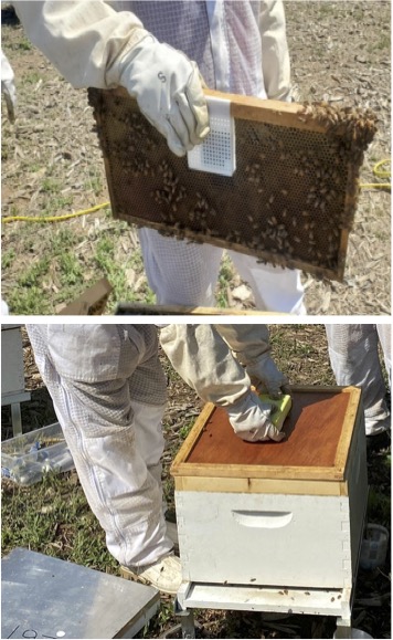
(a)

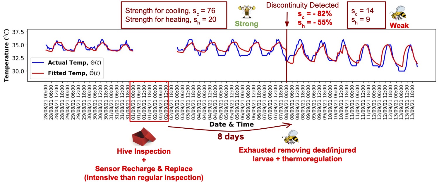
(b)

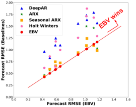
(c)

Figure 1: EBV at work: (a) deployed sensors (b) reconstruction and event detection (c) EBV wins on forecasting.

Method overview. We propose a method, EBV (Electronic Bee Veterinarian), specifically designed to monitor the hive temperature. We applied EBV to multiple real-time sequences collected from different hive settings and achieved reliable forecasts for several days ahead with a good fit (Figure 1(c), Details in Section 3.2), a lift of up to 49% in AUC over baselines (Figure 4); computation time of around 20 minutes for fitting two months of data, and segmentation coinciding with external events affecting bees’ thermoregulation ability (Figure 1(b), Details in Section 3.1).

Contributions. Specifically, the main contributions of this paper are summarized as follows:

• Principled: We propose a method, EBV comprised of (i) EBV_model, a novel model based on the thermal diffusion equation; control theory; and our novel ‘split’ P-controller idea (Section 2.3.1); and (ii) EBV_fit&cut, a segmentation algorithm (Section 2.3.3) based on EBV_model to estimate the number of cut-points where each cut represents a different hive condition. As bees follow the same mechanism to regulate hive temperature, our method is universally applicable regardless of region, season, and bee species.

• Effective: We use the proposed EBV_fit&cut for (i) fitting, (ii) forecasting, and (iii) segmentation to detect unexpected events. It performs well in terms of forecasting accuracy.

• Explainable: We can explain the current hive condition with the parameters (i.e., beehive strengths) measured and discontinuity detected by EBV_fit&cut.

• Scalable: Our method is scalable and hands-off, requiring no parameter tuning. It is applicable to all hives irrespective of size and population.

• Informative: Our experimental findings coincide with domain experts’ expectations: (i) bees in treated hives are less affected by intensive hive inspection; (ii) treated colonies have a higher strength to maintain thermoregulation than control ones, and (iii) heating a hive is easier than cooling it down  [8].

Reproducibility. Our implementation is open-sourced at https://github.com/rtenlab/EBeeVet. The dataset is available upon request.

2 Method & Technical Solution

2.1 Related Work

Beehive monitoring and analysis. Past systems collect in-hive microclimate parameters like temperature, humidity, and CO₂  [9, 10, 11, 12], sound signals  [13, 14], and visual bee activities using IR LEDs or cameras installed at the hive entrance  [15, 16]. Efforts have been made mostly to analyze sound signals to detect swarming events  [13, 14]. Attempts to analyze other in-hive data such as temperature to detect anomalies  [17, 18] are limited to arbitrary thresholds defined by domain specialist, rule-based, or simple autoencoders. All these approaches fail to provide causal relationships with colony health, lack robust evidence for analysis, and suffer from poor sensing quality or intermittent interruptions due to environmental conditions.

	Prior hive mon. [17, 18]	Trad. time series [22, 23]	Deep Learn. Tech. [24]	EBV (Ours)
domain-informative	✔			✔
effective		?	?	✔
explainable	?			✔
scalable		✔	?	✔

Table 1: EBV wins, fulfilling all the specifications. ‘?’ means ‘maybe, depending on implementation’.

Traditional time series forecasting. Time series have attracted huge research interest [19, 20, 21]. Classical methods, such as (i) autoregression (AR) based methods with exogenous variable [22], e.g., ARX/ARMAX/ARIMAX and seasonal ARX/ARMAX/ARIMAX, (ii) exponential smoothing models (ETS) [23], e.g., Holt-Winters, can be used for forecasting but they are neither domain-informative nor explainable. The hyperparameters of these models do not give any insights into the hive’s current condition.

Deep learning techniques. Such recent methods include Autogluon-Timeseries [24] (an open-source autoML library for time-series forecasting), DeepAR [25], Temporal Fusion Transformer [26], etc. The main drawback of these methods is the lack of explainability, despite recent attempts [27].

Contrast to existing literature. Existing hive health monitoring systems are supervised in nature based on either rule-based [18] or black-box methods [14]. To our knowledge, there exists no prior work to address this problem in an unsupervised manner. Also, none of them except EBV fulfill all specifications of Table 1.

2.2 DataSet and Experimental Setup

We have used a data set collected from August to September 2021 (late Summer) from an apiary in UC Riverside, CA, USA. This period in that region has very hot and dry climate conditions, with peak temperature exceeding $40^{\circ}$C. Such conditions can cause significant heat stress but doesn’t lead to colony collapse as long as bees are capable of managing in-hive temperature.

A total of ten homogeneous Langstroth hives with single-box brood chambers were used. They were divided equally into two groups for experimental purposes: control hives and treated hives. For each group, hives were selected randomly. Five control hives received no treatment throughout the experiment period. The remaining five hives were treated to combat extreme temperature by placing approximately six kilograms of ice on top of them when the environment temperature exceeded $35^{\circ}$C (Details in Section 3.1, Figure 2).

For data collection, we used a commercial multi-sensor device, Nordic Thingy:52 [28], which has wireless communication to transfer collected data. We recorded temperature per 20-minute interval for two months (August - September 2021). Every two weeks throughout that period, hives were opened twice: (i) for health evaluation and taking out the sensor device for battery recharging and (ii) for reinstalling the recharged device the next day. While all hives maintained the core temperature within $33-36^{\circ}$C, the control ones had a much higher deviation over several days, implying affected by heat stress. (Figure 5).

Sensor Placement. We kept the device inside a box so that bees do not build propolis around the hardware and affect its sensing ability. Each hive had two sensor devices placed in the following locations (Figure 1(a)):

1. Peripheral Area: On top of the outer frame near the food and honey preservation area.

2. Core Area: On the central frame near the brood area, where developing broods and the queen are present. The temperature of this area is crucial to hive health as developing broods are susceptible to heat stress, and healthy hives maintain the core area temperature between $33-36^{\circ}$C.

We also installed the sensor device in an empty Langstroth box. As that hive had no bees inside to regulate the core temperature, we consider the reference temperature to be the outer surface temperature of the hives, ${\Theta_{ext}(t)}$.

2.3 Proposed Method: EBV

Table  2 summarizes the symbols and their definitions used in the paper.

Symbols	Definitions
$\mathcal{D}$	Temperature dataset
$\mathcal{M}$	Model in Eqn.  (2.1)
$\mathcal{L(D|M)}$	Likelihood of $\mathcal{D}$ given $\mathcal{M}$
${\theta_{ideal}}$	Ideal core temperature
${\Theta_{ext}(t)}$	External temperature
${\Theta_{peri}(t)},{\Theta(t)}$	Hive’s Peripheral & Core temp.
${\theta_{ext}(t)}$	${\Theta_{ext}(t)}$ relative to ${\theta_{ideal}}$
${\theta_{peri}(t)},{\theta(t)}$	${\Theta_{peri}(t)},{\Theta(t)}$ relative to ${\theta_{ideal}}$
$\hat{\theta}(t)$	Fitted/forecasted ${\theta(t)}$ relative to ${\theta_{ideal}}$
${\Theta_{adj}(t)}$	Second surface temp. based on hive type
${s_{c}}$, ${s_{h}}$	Bees’ strength of cooling & heating

Table 2: Symbols & Definitions

2.3.1 Proposed Model: EBV_model.

We present our principled model, EBV_model, to monitor and forecast the hive core temperature ${\Theta(t)}$, given the outside temperature ${\Theta_{ext}(t)}$.

Lemma 2.1

Given the external temperature, ${\Theta_{ext}(t)}$, and the strengths ${s_{h}}$ and ${s_{c}}$ of honeybees for warming up and cooling down the hive, respectively, the hive core temperature, ${\Theta(t)}$, would obey:

(2.1)

where

$${\theta_{adj}(t)}=\begin{cases}{\theta_{ext}(t)},&\text{if $hive\ type=control$}\\ {\theta_{peri}(t)},&\text{if $hive\ type=treated$}.\end{cases}$$

Next, we provide the justification of our model, EBV_model (Eqn. 2.1) by using first principles: Thermal diffusion and Control theory.

2.3.2 Justification

Here, all temperatures are relative to the hive’s ideal core temperature, ${\theta_{ideal}}$, as bees efforts to keep the core temperature, ${\Theta(t)}$, within the normal range, depends on its deviation from ${\theta_{ideal}}$. It is worth noting that the ideal temperature ${\theta_{ideal}}$ is within $33-36^{\circ}$C but the exact value can vary slightly within this range, from day to day and from hive to hive, due to several reasons, such as hive size, population, and season.

To take into account the effect of treatment, we consider two types of hive surface temperatures: top (${\Theta_{adj}(t)}$) and the rest surfaces (${\Theta_{ext}(t)}$). For control hives, we assume all surfaces share the same ${\Theta_{ext}(t)}$ since all of them directly face the outside. For treated hives, there was ice on the top surface on hot days, and the top surface temperature, ${\Theta_{adj}(t)}$, would be different from the rest surfaces and can be obtained by the sensor installed in the peripheral area, ${\Theta_{peri}(t)}$. Based on this, we derive Eqn. (2.1) in the following steps.

Step 1: Physics - Thermal Diffusion. The first term in Eqn. (2.1) is due to heat transfer: for an empty hive, the rate of change in hive core temperature, $\frac{\partial{{\theta(t)}}}{\partial t}$ obeys the thermal diffusion model [29],

$$\boxed{\nabla^{2}{\theta}=\frac{\partial^{2}{\theta}}{\partial x^{2}}+\frac{\partial^{2}{\theta}}{\partial y^{2}}+\frac{\partial^{2}{\theta}}{\partial z^{2}}\propto\frac{\partial{\theta}}{\partial t}}$$

So, we can define $\frac{\partial{{\theta(t)}}}{\partial t}={\theta_{ext}(t)}+{\theta_{adj}(t)}-2{\theta(t)}$.

Step 2: Control Theory - (split) P-controller. The second term is the feedback loop [30]: when the hive core temperature, ${\Theta(t)}$ is away from ideal core temperature ${\theta_{ideal}}$, bees try to bring it to zero with strengths ${s_{c}}$ and ${s_{h}}$ and their efforts are proportional to ${\theta(t)}$ i.e., if bees are left alone,

$$\frac{\partial{{\theta(t)}}}{\partial t}=\begin{cases}-{s_{c}}{\theta(t)},&\mathrm{if~{}}{\theta_{ext}(t)}\geq 0.\\ +{s_{h}}{\theta(t)},&\mathrm{otherwise}.\end{cases}$$

Notice that we propose to have a split in the standard proportional (P) controllers: the bees have different ability to cool (${s_{c}}$: when ${\Theta_{ext}(t)}$ goes above ${\theta_{ideal}}$) and different ability to heat (${s_{h}}$: when ${\Theta_{ext}(t)}$ goes below ${\theta_{ideal}}$) - this is exactly what we call split P-controller. We have followed the sign convention: negative work for heating and positive work for cooling. Combining these two effects makes the equation the same as Eqn. (2.1).

Our goal is to find out such cooling and heating strengths ${s_{c}}$, ${s_{h}}$, and ${\theta_{ideal}}$ that best reconstructs ${\Theta(t)}$, given ${\Theta_{ext}(t)}$ and ${\Theta_{adj}(t)}$.

2.3.3 Proposed Algorithm: EBV_fit&cut.

Based on EBV_model, we develop a segmentation algorithm to find out a set of segments and their parameters by penalizing model complexity. The cut-points spot discontinuity corresponding to events affecting bees’ thermoregulation ability. We use AIC (Akaike Information Criterion) to measure the goodness of fit of our algorithm. We want to minimize the following equation:

(2.2) $$AIC=-2ln\mathcal{L}(\mathcal{D}|\mathcal{M})+2(m+(m+1)p)$$

where $\mathcal{L}(\mathcal{D}|\mathcal{M})$ is the likelihood of data $\mathcal{D}$ given the model $\mathcal{M}$ described in Eqn. (2.3) and $m,p\,(=3)$ represent the number of cut points and the number of parameters for each segment respectively. $\mathcal{L}(\mathcal{D}|\mathcal{M})$ is given by:

(2.3) $$\mathcal{L}(\mathcal{D}|\mathcal{M})=\prod_{i=1}^{N}f(\Theta[i]-\hat{\Theta}[i])$$

where $f(.)$ is the pdf of a continuous normal random variable, and $N$ is the number of total time ticks.

We want to find the combination of segments and corresponding parameters, $\{{s_{c}},{s_{h}},{\theta_{ideal}}\}$ that minimizes Eqn.  (2.2) and outputs the best-fitted core temperature, ${\hat{\Theta}(t)}$. Algorithm 1 demonstrates EBV_fit&cut, the implementation of EBV_model for curve fitting and segmentation.

Input: $\mathcal{D}=\{\mathcal{{\theta_{E}}},\mathcal{{\theta_{P}}},\mathcal{{\theta}}\}$

Output: {$\mathcal{{CP}}$, $\mathbfcal{X}$}

1

2/* Fitting: compute ${\hat{\Theta}(t)}$ */

3for each pair $(e,d)\in(\mathcal{P},\mathcal{D})$ do  sol. Eqn. (2.1)

4

5/*Segmentation and finding cut points*/

6$j\leftarrow 1,\mathcal{{CP}}\leftarrow\{0,n\},\mathbfcal{X}\leftarrow\emptyset$

7while j $<$ n  do

8       for each point, $p\in\{\mathcal{D}-\mathcal{{CP}}\}$ do

9             $cp\leftarrow\{\mathcal{{CP}}\}\cup p$ //set of cut-points

10            for i = 0 to length($\mathcal{{CP}}$) do

11                   Create Segment $s[i]\leftarrow\mathcal{D}[cp[i]:cp[i+1]]$

12                  Fit and choose $\mathcal{P}_{best}\leftarrow\mathcal{P}_{RMSE_{min}}$

13            

14            Calculate $\mathcal{L}({\Theta(t)},\hat{\Theta}(t))$ /*Eqn. (2.3)*/

15      

16      Choose $\mathcal{L}_{min}({\Theta(t)},\hat{\Theta}(t))$, and $\mathcal{P}_{\mathcal{L}_{min}}$

17      $\{\mathcal{{CP}},\mathbfcal{X}\}\leftarrow\{\{\mathcal{{CP}}\}\cup p_{\mathcal{L}_{min}},\{\mathbfcal{X}\}\cup\mathcal{P}_{\mathcal{L}_{min}}\}$

18      $j\leftarrow j+1$

19

Algorithm 1 EBV_fit&cut

EBV_fit&cut takes $\mathcal{D}=\{\mathcal{{\theta_{E}}},\mathcal{{\theta_{P}}},\mathcal{{\theta}}\}$ as input and $\mathcal{CP}=\{cp_{1},cp_{2},...cp_{m}\}$, $\mathbfcal{X}=\{\mathcal{X}_{1},\mathcal{X}_{2},...\mathcal{X}_{m+1}\}$ as output:

• $\mathcal{D}=\{\mathcal{{\theta_{E}}},\mathcal{{\theta_{P}}},\mathcal{{\theta}}\}$ is the dataset for a hive. Here, $\mathcal{\theta_{E}}$, $\mathcal{\theta_{P}}$, $\mathcal{\theta}$ are sets of daily external, peripheral and core temperature sequences over the experiment period.

• $\mathcal{CP}=\{cp_{1},cp_{2},...cp_{m}\}$ and $\mathbfcal{X}=\{\mathcal{X}_{1},\mathcal{X}_{2},...\mathcal{X}_{m+1}\}$ are the sets of cut point locations and $\{{s_{c}},{s_{h}},{\theta_{ideal}}\}$ respectively, where $m$ is the number of cut points i.e., $m\leq n$, $n$ is the number of daily sequences.

Fitting. (lines 1 to 1) We use Levenberg-Marquardt (LM) optimization for faster convergence (other kinds of optimization or linear search can also be used) considering the following constraints for the search space $\mathcal{P}=\{\mathcal{S_{C}},\mathcal{S_{H}},\mathcal{\theta_{I}}\}$ (line 1).

1. $\mathcal{S_{C}}\land\mathcal{S_{H}}=[0,s_{\infty}]$ are the search space for bees’ cooling and heating strength, ${s_{c}}$ and ${s_{h}}$ respectively. Normally, $\mathcal{S_{C}}$ and $\mathcal{S_{H}}$ vary between [0,50] (Details in Section 3.3) with a few exceptions. So, the upper limit $s_{\infty}$ can be any value above 50.

2. $\mathcal{\theta_{I}}=[\theta_{ideal}^{lower},\theta_{ideal}^{upper}]$ is the search space for ${\theta_{ideal}}$ that can be anywhere between $33-36^{\circ}$C for healthy hives and go outside this range for unhealthy ones. We assumed the range to be $(33-36)\pm 2^{\circ}$C.

There can be two instances when we cannot calculate the strength of bees and do either linear interpolation or forward/backward filling, considering strength(s) as a continuous variable(s).:

• Case 1: ${\Theta(t)}$ is almost constant the whole day (${s_{c}}$, ${s_{h}}$ will reach the upper limit).

• Case 2: ${\Theta(t)}$ is below/above ${\theta_{ideal}}$ the whole day(${s_{c}}$/${s_{h}}$ will be zero or any other constant).

Segmentation and finding cut-points. (lines 1 to  1) For this part, we use the following notations.

• $\mathcal{L}=\{l_{1},l_{2},...l_{n}\}$ is the set of likelihoods for different cut-points positions and $\mathcal{L}_{min}$ is the minimum of $\mathcal{L}$.

• $\mathcal{P}_{RMSE_{min}}$ and $\mathcal{P}_{\mathcal{L}_{min}}$ is the parameters $\mathcal{X}=\{{s_{c}},{s_{h}},{\theta_{ideal}}\}$ for each segment that gives minimum RMSE and AIC for $\mathcal{D}$.

For segmentation, we follow a greedy approach. Let’s begin with the simplest case: a single cut-point search with two segments (i.e.,  $\mathcal{S}_{1}$ and $\mathcal{S}_{2}$) for a given dataset $\mathcal{D}$. Each segment will have its respective parameters, $\mathcal{X}_{i}=\{{s_{c}},{s_{h}},{\theta_{ideal}}\}_{i}$ for best reconstruction. We start with the cut-point position, $cp=1$ and iterate till $n$. For each cut-point, we will have $\{(\mathcal{S}_{1},\mathcal{X}_{1}),(\mathcal{S}_{2},\mathcal{X}_{2})\}$ and $\mathcal{L}$ for $\mathcal{D}$. We will choose $\mathcal{{CP}}=\{cp_{1}\}$ with $\mathcal{L}_{min}$. How about a second one? We will repeat the above process, excluding $cp_{1}$ from our search. Then, we will have $\mathcal{{CP}}=\{cp_{1},cp_{2}\}$ and repeat the same process for the next one till we find reconstruction with minimum AIC.

Reconstruction using more segments will be closer to the original reconstruction. As will be shown in Figure 5, we get the best fit if each sequence is considered independent of the other i.e., $n$ sets of $\mathcal{X}$ for n sequences. But more segments also increase the chances of detecting cuts with no significant changes in $\mathcal{X}$. In segmentation, we aim to reduce the model complexity by reducing the number of $\mathcal{X}$s. Thus, instead of considering minimum AIC, we use the combination of segments and parameters that gives 10% higher AIC than the minimum one [21]. The experimental results in Section 3.1 demonstrate that our assumption is reasonable.

3 Empirical Evaluation

This section presents the effectiveness of our proposed method, EBV, using our collected datasets and experiments designed to ensure the following:

1. Effectiveness: How accurately does our proposed method EBV detect events affecting hive health and forecast the core temperature, ${\Theta(t)}$? (Sec. 3.1 & 3.2)

2. Explainability: Can EBV explain the change in bee strengths and the effect of corresponding events in detected segments? (Sec. 3.3)

3. Scalability: Does our model perform linearly in time? (Sec. 3.4)

4. Observations: Do the observations based on our experiments coincide with the domain experts’ expectations? (Sec. 3.5)

All experiments are done on a Dell XPS 15 laptop with an Intel i9 processor and 32GB memory. We used averaged hourly data for all experiments as the change in temperature is noticeable if considered hourly. There are missing data points due to the nature of real-world data collection, e.g., sensors not working properly, beekeepers’ intervention for inspection, etc. However, no interpolation is done since ${EBV\textsubscript{fit\&cut}}$ is robust to handling missing values. Due to space constraints, we present one example hive from each hive setting in this section, but our findings are applicable to all hives used during the experiment.

3.1 Q1 - Effectiveness: Event-detection.

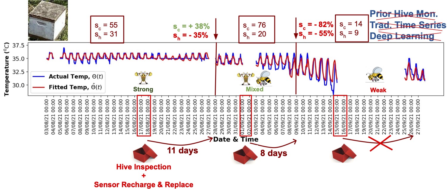
(a)

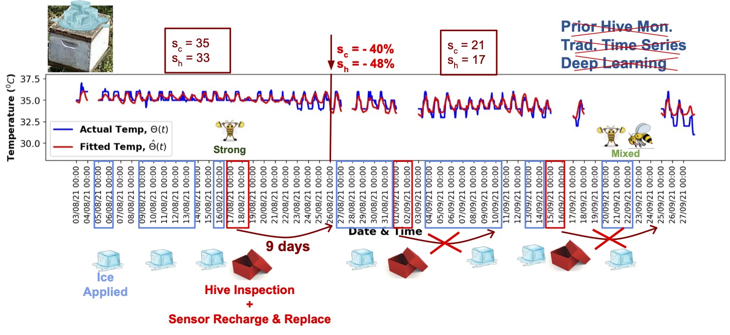
(b)

Figure 2: EBV is effective & explainable: Accurate segments: EBV_fit&cut fits (red line) the data (blue line) well and finds cut-points (brown vertical line) followed by unexpected events (red boxes: intensive hive inspection, sensor recharge and replace). Notice that the baselines are not applicable (cannot do segmentation).

Experimental Setup. Frames were taken out of hives twice in two days during every inspection to recharge and replace sensors installed inside (Section  2.2). It takes more time than usual and thus induces more stress and damage to bees and larvae. We refer to this type of inspection as intensive compared to regular ones. All hives were opened on the same days: 17-18 August, 1-2 September, and 15-16 September (marked by open red boxes: intensive inspection). Also, ice treatments during hot days for treated hives are marked by blue boxes with ice symbols (Figure  2). We want to see if EBV_fit&cut is able to detect changes in ${\Theta(t)}$ following the inspections.

1. Intensive hive inspections: To maintain hive hygiene and population growth, bees need to remove larvae affected during inspection and reestablish homeostasis. For stressed hives, maintaining thermoregulation and cleanliness at the same time can lead to a noticeable increase in fluctuation in ${\Theta(t)}$ within 9-10 days following the inspection.

2. Effect of ice treatment: Domain experts expect ice treatment during hot days will help maintain stress and thermoregulation following intensive inspections in the long run.

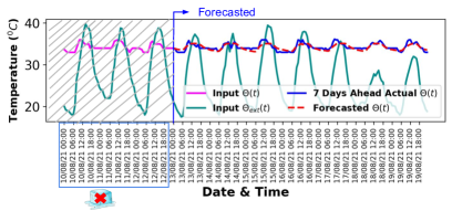
(a)

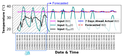
(b)

Figure 3: EBV forecasts well: The seven days ahead forecasting (dotted red line) is close to the actual core temperature (solid blue line).

Results. EBV_fit&cut detected $n=2$ and $n=1$ cut-points and corresponding parameters for each segment (brown vertical line in Figure 2) for the control and treated hive, respectively. The reconstructed curve (red line) by EBV_fit&cut is well aligned with the recorded ${\Theta(t)}$ (blue line).

For the control hive (Figure 2(a)), EBV_fit&cut detected cut-points on 28 August and 9 September: 11 and 8 days following the first and second inspection, respectively. We suspect it is correlated to hive cleaning (affected larvae removal) and re-establishing homeostasis after intensive inspection. No cut-point was detected after the openings on 15-16 September. The reason might be the recorded data length after the inspection: too short to detect discontinuity.

For the treated hive, EBV_fit&cut detected a cut-point (Figure 2(b)) on 26 August: 9 days following the first inspection. No cut-points were detected after the next two inspections. This indicates bees in the treated hive were good at managing the aftereffects of intensive inspections. We strongly suspect this is a result of the positive cumulative effect of ice treatment over time.

In summary, our algorithm EBV_fit&cut detected a total of 9 cut-points for 15 inspections (3 per hive) of control hives and 5 cut-points for 15 inspections of treated ones. There were no false positives, and the detected events had ecological significance (Section 3.3).

3.2 Q1 - Effectiveness: Forecasting

Experimental Setup. For each trial, we use three days of temperature sequences (endogenous variable: ${\Theta(t)}$ and exogenous variable: ${\Theta_{ext}(t)}$, ${\Theta_{adj}(t)}$) as inputs and forecast ${\Theta(t)}$ hourly for the next seven days, given ${\Theta_{ext}(t)}$ for the forecasting period. The forecasted core temperature is compared against the actual core temperature using RMSE: RMSE = $\sqrt{\frac{\sum_{i=1}^{K}(\Theta[i]-\hat{\Theta}[i])^{2}}{K}}$, where $K$ is the number of forecasted time-ticks and $\hat{\Theta}[i]$ is the forecasted value at $i$-th time-tick.

Baselines. To demonstrate the effectiveness of EBV in forecasting, we compared it to the state-of-the-art time series forecasting models ARX, seasonal ARX [22], Holt-Winters [23], and DeepAR from Autogluon [24]. We followed standard practice to determine (i) the order of ARX and seasonal ARX: AIC [31], and (ii) the hyperparameters of the Holt-Winters method: additive trend and seasonality and non-linear optimization. For DeepAR, we used 2 RNN layers with 40 cells for each and a learning rate of 0.001. As Autogluon (DeepAR) requires the input sequence length to be greater than twice the length of the forecasting period, we recursively forecast seven days ahead for three days of input data.

For EBV, we use estimated parameters (${s_{c}}$, ${s_{h}}$ and ${\theta_{ideal}}$) from the input sequences along with ${\Theta_{ext}(t)}$ for the next seven days to forecast ${\Theta(t)}$ for that time period.

Results. Figure 3 demonstrates examples of the seven-day-ahead forecasting of ${\Theta(t)}$ (13-19 August 2021) using three days’ temperature sequences (10-12 August 2021) as inputs. The magenta, black, and cyan lines represent the input ${\Theta(t)}$, ${\Theta_{ext}(t)}$, and ${\Theta_{peri}(t)}$ (for the treated hive), respectively. As can be seen, the forecasted core temperature sequence (dashed red line) is very close to the actual one (blue line), demonstrating the effectiveness of our method.

Accuracy. Figure 4 shows the comparison of the average RMSE of all sequences among baselines and EBV for different hive types. EBV shows an average improvement of up to 49% over baselines in terms of accuracy. The average RMSEs for all experimental hives are also reported in Figure 1(c). Each point corresponds to a (hive-id, forecasting method) pair. We show that all points (except a few) fall in the upper left region of the red line (average RMSEs of EBV), indicating better forecasting accuracy of EBV than baselines.

ARX and seasonal ARX do good forecasting (second-best), but our proposed method, EBV has an additional advantage over any other method: parameters of baselines are not explainable whereas, EBV can better explain the bee strengths with the parameters ${s_{c}}$ and ${s_{h}}$. Also, the intuition of EBV conforms to the domain experts’ expectations: increased fluctuation in core temperature ${\Theta(t)}$ indicates decreased bee strengths (${s_{c}},{s_{h}}$) to maintain ${\Theta(t)}$ and deteriorating hive health (Figure 5).

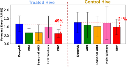
Figure 4: EBV wins against baseline in terms of forecasting accuracy (up to 49% improvement). Error bars show 1 standard deviation.

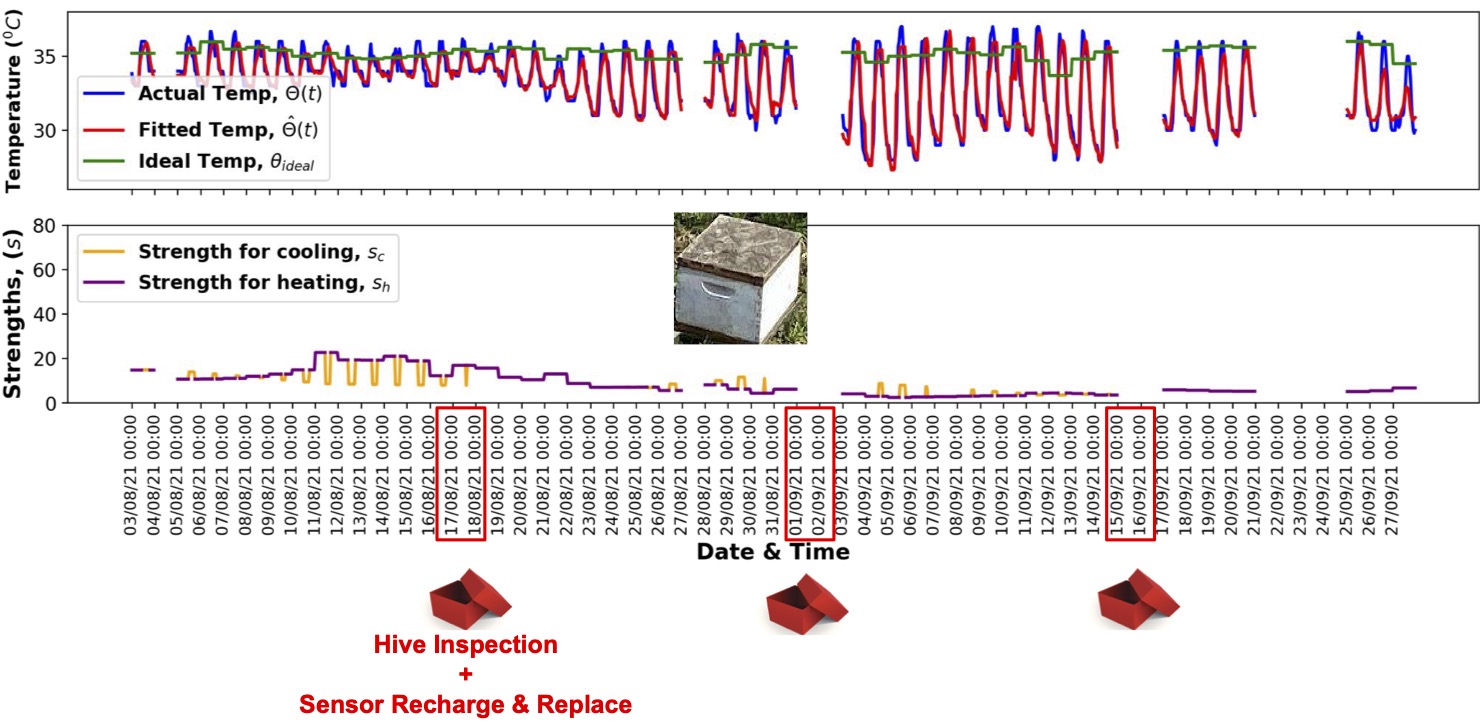
(a)

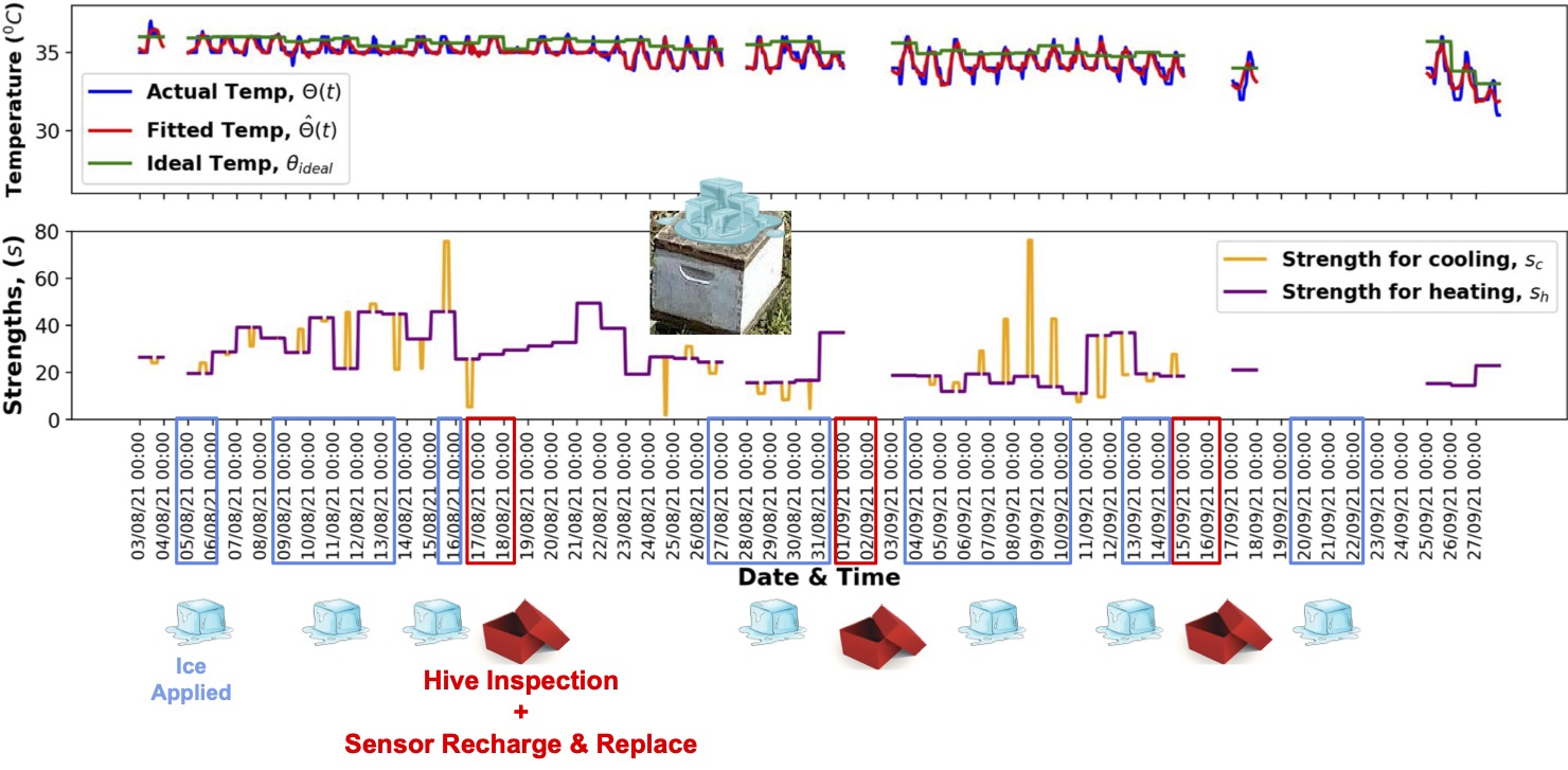
(b)

Figure 5: EBV captures the effect of ice treatment: Bees in treated hives are stronger than the ones in control hives.

3.3 Q2 - Explainability

As mentioned in Section  3.1, each cutpoint and the change in parameters between adjacent segments (Figure 2) are indications of events affecting thermoregulation and hive health.

Effect of intensive hive inspection. According to domain experts, the effect of intense hive inspections is reflected through the change in ${\Theta(t)}$ within a few days following the inspection.

For the control hive (Figure 2(a)), ${s_{c}}$ went up by 38% while the ${s_{h}}$ went down by 35% after the first cut-point. It indicates bees’ struggle to manage the cleanliness and ${\Theta(t)}$ following hive inspection and sensor replacement. After the second cut-point, both ${s_{c}}$ and ${s_{h}}$ decreased drastically by 82% and 55%, indicating severely affected thermoregulation and weak bees.

Effect of ice treatment on thermoregulation. Figure 5 shows the reconstructed curves (red line) for the recorded ${\Theta(t)}$ (blue line) assuming daily fluctuation in parameters, ${\theta_{ideal}}$ (green line: top graphs) and bee strengths, ${s_{c}}$, ${s_{h}}$ (orange and purple lines: bottom graphs) over the experiment period.

In the bottom graphs, we can observe (i) the low strength of bees (in the range of [3,25]; Figure 5(a)) in control hives compared to treated ones (mostly in the range of [20,80]; Figure 5(b)), (ii) comparatively drastic change in bee strengths (${s_{c}},{s_{h}}$) and increased fluctuation in ${\Theta(t)}$ of the control hive, following intensive inspection.

For the treated hive in Figure 2(b), EBV_fit&cut detects only one cut-point (only after the first inspection) with a reduction of 40% and 48% in ${s_{c}}$ and ${s_{h}}$ respectively. No parameter changes were detected for the following two events. This indicates that the bees were healthy enough to combat the aftereffect of intensive inspections and control the fluctuation in ${\Theta(t)}$.

These results coincide with domain experts’ expectations: ice packs during hot days will help bees regulate ${\Theta(t)}$ and manage the aftereffects of intensive inspections.

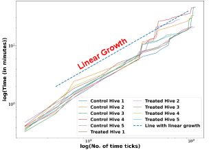
Figure 6: EBV is linear with input size : growth parallel to diagonal.

3.4 Q3 - Scalability

Our proposed model, EBV_model is fast, and takes only about 20 minutes on average to process and fit two months of data for a well-defined search space on the laptop described above. EBV_model is easily parallelizable as the data from each day and each hive is independent. We conclude with the following lemmas.

Lemma 3.1

Reconstruction using EBV_model is linear in time, i.e., for $t$ time ticks, the time complexity of reconstruction is O(t).

• We use Levenberg-Marquardt (LM) optimization, and the time for convergence is linear with the number of time ticks. $\quad\blacksquare$   

All (solid) lines in Figure  6 (time to reconstruct two months of data for experimental hives in logarithmic scale) are parallel to the reference line of linear growth (dashed blue line), indicating scalability.

Lemma 3.2

Segmentation using EBV_fit&cut is linear in time, i.e., the time complexity for finding m segments in a given dataset $\mathcal{D}$ with t time ticks is $O(t\times m)$.

• For a time sequence with $t$ time ticks, we use a greedy algorithm to find the $m$ cut-points. Each cut-point requires one scan of the sequence $O(m)$, and thus the complexity is $O(t\times m)$. $\quad\blacksquare$   

3.5 Q4 - Observations

Effect of intensive hive inspection. As described in Section 3.1, our algorithm EBV_fit&cut detected 80% more cut-points in total for control hives than for treated ones for the same number (3 per hive) and type of (intensive) inspection. That is:

Observation 1

Control (= untreated) hives suffer more from intensive hive inspections.

That is, control hives show more discontinuities and less control over their temperature.

Effect of ice treatment on thermoregulation. We demonstrate the distribution of bee strengths over the experimental period from different hive settings (2021 Data) as a logarithmic scatter plot of ${s_{c}}$ vs ${s_{h}}$ (cooling-strength vs heating-strength) in Figure 7. Every data point corresponds to a (hive-id, timestamp) pair.

Notice that bees in control (= untreated) hives show a lower ability to heat and cool their hives.

Observation 2

Bees in treated hives are stronger, i.e., they have better thermoregulation ability than the ones in control hives.

Difference in strength during heating and cooling. The gray line in Figure 7 divides the graph into two regions: (i) upper left: heating is easier than cooling (ii) lower right: cooling is easier than heating. Notice that most data points fall into the upper left region, coinciding with the domain expert’s expectation:

Observation 3

Heating a hive is easier than cooling it down.

Figure 7: EBV spot differences: heating/cooling strength ${s_{c}}$ vs ${s_{h}}$ in logarithmic scale. It corroborates that bees in treated hives are stronger.

4 Conclusions, Significance and Impact

We proposed EBV (Electronic Bee-Veterinarian) to help beekeepers monitor and analyze the health of their hives and take preventive actions.

EBV is (a) principled, using physics (thermal diffusion equations) and control theory (feedback-loop ‘split’ P-controllers); (b) interpretable by beekeepers with only a few parameters (i.e., bee strengths for heating and cooling); (c) effective in fitting, forecasting, and detecting events affecting hive health; (d) scalable; and (e) informative, agreeing with experts’ expectations.

Significance. Honeybees are vital for pollination of crops. Novel monitoring tools to safeguard bees are a matter of global urgency. Our proposed model, EBV will be of broad interest to beekeepers, growers, and researchers studying all facets of pollinator health all over the world. A reliable model with confirmed analytic capabilities will be a game changer for the global beekeeping industry.

Impact. A preliminary version of our model received positive feedback from local beekeepers at the UC Riverside Bee Health conference in 2022 [5]. We are in constant contact with them and co-organizing yearly events with CIBER to keep them updated about our endeavor.

Reproducibility. As mentioned in Section 1, our code is on GitHub: https://github.com/rtenlab/EBeeVet; and our collected dataset is available upon request.

5 Acknowledgments

This work was partially supported by a UC Multicampus Research Programs and Initiatives (MRPI) award (# M21PR2306). We extend special thanks to Jamison Scholer for his help in managing the bee hives and Mohsen Karimi for his help in collecting the data.

References

- [1] Elisabeth Eilers et al. Contribution of Pollinator-Mediated Crops to Nutrients in the Human Food Supply, PloS one. 6. e21363 (2011).
- [2] Simon G Potts et al. Safeguarding pollinators and their values to human well-being. Nature. 2016 Dec 8;540(7632):220-229.
- [3] Dan Aurell et al. United States Honey Bee Colony Losses 2021-2022: Preliminary Results from the Bee Informed Partnership, 2022, url.
- [4] Matthew L Forister et al. Declines in insect abundance and diversity: We know enough to act now, Conservation Science and Practice. 2019; 1:e80.
- [5] Center for Integrative Bee Research (CIBER), Ciber Bee Health Conference at UC Riverside, 2022. url.
- [6] Marco Kleinhenz et al. Hot bees in empty broodnest cells: heating from within, The Journal of experimental biology 206 (12 2003), 4217–31.
- [7] Markus Petz et al. Respiration of individual honeybee larvae in relation to age and ambient temperature, Journal of Comparative Physiology B 174 (10 2004), 511–518.
- [8] Hasila Jarimi et al. A Review on Thermoregulation Techniques in Honey Bees’ (Apis Mellifera) Beehive Microclimate and Its Similarities to the Heating and Cooling Management in Buildings, Future Cities and Environment 6 (08 2020), 7.
- [9] Stefania Cecchi et al. Smart Sensor-Based Measurement System for Advanced Bee Hive Monitoring, Sensors 20 (05 2020), 2726.
- [10] Douglas Santiago Kridi et al. Application of wireless sensor networks for beehive monitoring and in-hive thermal patterns detection, Comput. Electron. Agric. 127 (09 2016), 221–235.
- [11] V Pandimurugan et al. IoT based Smart Beekeeping Monitoring system for beekeepers in India, In 2021 4th ICCCT, IEEE, Chennai, India.
- [12] Chau-Chung Songa et al. Development of Intelligent Beehive and Network Monitoring System for Bee Ecology, ICAROB2022, 27 (01 2022).
- [13] Fiona Edwards Murphy et al. An automatic, wireless audio recording node for analysis of beehives, In 2015 26th ISSC, IEEE, Carlow, Ireland.
- [14] Tony Zhang et al. Semi-Supervised Audio Representation Learning for Modeling Beehive Strengths, CoRR abs/2105.10536 (05 2021).
- [15] Joe-Air Jiang et al. A WSN-based automatic monitoring system for the foraging behavior of honey bees and environmental factors of beehives, Comput. Elect. Agric. 123 (04 2016), 304–318.
- [16] Cheng Yang et al. A Model for Pollen Measurement Using Video Monitoring of Honey Bees, Sensing and Imaging 19, 2 (12 2017).
- [17] Padraig Davidson et al. Anomaly Detection in Beehives using Deep Recurrent Autoencoders, CoRR abs/2003.04576 (2020).
- [18] Fiona Edwards-Murphy et al. b+WSN: Smart beehive with preliminary decision tree analysis for agriculture and honey bee health monitoring, Comput. Electr. Agric. 124 (2016), 211–219.
- [19] Leman Akoglu et al. Event detection in time series of mo- bile communication graphs, 27th Army Sci Conf 2 (01 2010).
- [20] Lexiang Ye et al. Time Series Shapelets: A New Primitive for Data Mining In Proceedings of the 15th ACM SIGKDD 2009.
- [21] Yasuko Matsubara et al. AutoPlait: Automatic Mining of Co-Evolving Time Sequences, In Proceedings of the 2014 ACM SIGMOD.
- [22] George E. Box et al. Time series analysis: forecasting and control, John Wiley & Sons, 2015.
- [23] James D. Hamilton, Time series analysis, volume 2, Princeton university press Princeton, 1994.
- [24] Caner Turkmen et al. Easy and accurate forecasting with AutoGluon-TimeSeries, 2022. url.
- [25] Salinas David et al. DeepAR: Probabilistic forecasting with autoregressive recurrent networks, International Journal of Forecasting 36. 3 (2020): 1181-1191.
- [26] Lim Bryan et al. Temporal Fusion Transformers for interpretable multi-horizon time series forecasting, International Journal of Forecasting 37.4 (2021): 1748-1764.
- [27] Waddah Saeed et al. Explainable AI (XAI): A systematic meta-survey of current challenges and future opportunities, International Journal of Forecasting 37.4 (2021): 1748-1764.
- [28] Nordic Semiconductor, Nordic Thingy:52, url.
- [29] J. Crank, The mathematics of diffusion, Oxford University Press, 1975.
- [30] Norman S. Nise, Control Systems Engineering, John Wiley & Sons, 2019.
- [31] Clifford M. Hurvich et al. A corrected akaike information criterion for vector autoregressive model selection., Journal of time series analysis, 14(3):271– 279, 1993.