Distributional Off-policy Evaluation with Bellman Residual Minimization

Abstract

We consider the problem of distributional off-policy evaluation which serves as the foundation of many distributional reinforcement learning (DRL) algorithms. In contrast to most existing works (that rely on supremum-extended statistical distances such as supremum-Wasserstein distance), we study the expectation-extended statistical distance for quantifying the distributional Bellman residuals and show that it can upper bound the expected error of estimating the return distribution. Based on this appealing property, by extending the framework of Bellman residual minimization to DRL, we propose a method called Energy Bellman Residual Minimizer (EBRM) to estimate the return distribution. We establish a finite-sample error bound for the EBRM estimator under the realizability assumption. Furthermore, we introduce a variant of our method based on a multi-step bootstrapping procedure to enable multi-step extension. By selecting an appropriate step level, we obtain a better error bound for this variant of EBRM compared to a single-step EBRM, under some non-realizability settings. Finally, we demonstrate the superior performance of our method through simulation studies, comparing with several existing methods.

1 Introduction

In reinforcement learning (RL), the cumulative (discounted) reward, also known as the return, is a crucial quantity for evaluating the performance of a policy. Most existing RL methods only focus on the expectation of the return distribution. Bellemare have extended the focus to the whole return distribution, and they introduced a distributional RL (DRL) algorithm (hereafter called Categorical algorithm [1]) that achieves a considerably better performance in Atari games than expectation-oriented Deep-Q Networks [11]. This has sparked significant interests among the RL community, and was later followed by a series of quantile-based methods including QRDQN, QRTD [6], IQN [5], FQF [27], EDRL [17] and particle-based methods including MMDRL [15], SinkhornDRL [20], MD3QN [28]. In this paper, we consider the problem of off-policy evaluation in DRL, i.e., estimating the (conditional) return distribution of a target policy based on the offline setting.

Despite their competitive performances, distributional RL methods are significantly underdeveloped compared with the traditional expectation-based RL, especially in the theoretical development under the offline setting. All aforementioned methods are motivated by supremum-extended distances due to the contraction property (see (3) below), but their algorithms essentially minimize an objective function based on expectation-extended distance (see (5)), as summarized in the column “Distance Mismatch” of Table 1. This leads to a theory-practice gap.

Moreover, most of these work do not provide any statistical guarantee such as the convergence rates of their estimators. We note that Rowland established the consistency of their estimator, but no error bound is provided [16]. In terms of statistical analysis, a very recent work FLE [26] only offers error bound analysis of their estimator for the marginal distribution of return, which makes it difficult to be developed towards policy learning. In addition, their analysis is based on a strong condition called completeness, which in general significantly restricts model choices of return distributions and excludes the non-realizable scenario. Even when transition probability is well estimated, non-realizability may still happen, especially when a parametric model of the return distributions is used.

This paper proposes a novel estimator, which we call Energy Bellman Residual Minimizer (EBRM), based on the idea of Bellman residual minimization for estimating the conditional distribution of the return in the offline setting. Table 1 provides some key comparisons between our method and some existing works. More details are given in Table 3 in the Appendix D.1. Finally, we summarize our contributions as follows. (1) We provide theoretical foundation of the application of expectation-extended distance for Bellman residual minimization in DRL. Not only does this theoretical result support the proposed method, but it also provides theoretical justification for other existing methods, as explained in Section 2.3. (2) We develop a novel distributional off-policy evaluation method (EBRM), together with its finite-sample error bound. See Section 3. (3) We further develop a multi-step extension of EBRM for non-realizabile settings in Section 4. We also establish the corresponding finite-sample error bound under the non-realizable setting. (4) Our numerical experiments in Section 5 demonstrate the strong performance of EBRM compared with some baseline methods.

Table 1: Comparison among DRL methods for off-policy evaluation.

	Distance	Statistical	Non-	Multi-
Method	match	error bound	realizable	dimension
Categorical [1]	✗	✗	NA	✓
QRTD [6]	✗	✗	NA	✗
IQN [5]	✗	✗	NA	✗
FQF [27]	✗	✗	NA	✗
EDRL [17]	✗	✗	NA	✗
MMDRL [15]	✗	✗	NA	✓
SinkhornDRL [20]	✗	✗	NA	✓
MD3QN [28]	✗	✗	NA	✓
FLE [26]	✓	✓	NA	✓
EBRM (our method)	✓	✓	✓	✓

2 Off-policy Evaluation Based on Bellman Equation

2.1 Background

We consider an off-policy evaluation (OPE) problem under the framework of infinite-horizon Markov Decision Process (MDP), which is characterized by a state space $\mathcal{S}$, a discrete action space $\mathcal{A}$, and a transition kernel $p:\mathcal{S}\times\mathcal{A}\to\mathcal{P}(\mathbb{R}^{d}\times\mathcal{S})$ with $d\geq 1$ and $\mathcal{P}(\mathcal{X})$ denoting the class of probability measures over a generic space $\mathcal{X}$. In other words, $p$ defines a joint distribution of a $d$-dimensional immediate reward and the next state conditioned on a state-action pair. At each time point, an action is chosen by the agent based on the current state according to some (stochastic) policy, which is a mapping from $\mathcal{S}$ to $\mathcal{P}(\mathcal{A})$. A trajectory generated by such an MDP can be written as $\{S^{(t)},A^{(t)},R^{(t+1)}\}_{t\geq 0}$. The return variable is defined as $Z:=\sum_{t=1}^{\infty}\gamma^{t-1}R^{(t)}$ with $\gamma\in[0,1)$ being a discount factor, based on which we can evaluate the performance of some target policy $\pi$.

OPE is different from on-policy evaluation in that the data are collected by using a different policy called behavior policy $b$, other than the target policy $\pi$ that we want to evaluate. Therefore, OPE naturally involves an issue of distributional shift. Traditional OPE methods are mainly focused on estimating the expectation of the return $Z$ under the target policy $\pi$, whereas DRL aims to estimate the whole distribution of $Z$. In DRL, letting $\mathcal{L}(X)$ be the probability measure of some random variable (or vector) $X$, our target is to estimate the collection of return distributions conditioned on different initial state-action pairs $(S^{(0)},A^{(0)})=(s,a)$:

$$\Upsilon_{\pi}(s,a):=\mathcal{L}\bigg{(}\sum_{t=1}^{\infty}\gamma^{t-1}R^{(t)}\bigg{)},\quad\text{where }(R^{(t+1)},S^{(t+1)})\sim p(\cdot|S^{(t)},A^{(t)}),\ A^{(t+1)}\sim\pi(\cdot|S^{(t+1)}),$$

collectively written as $\Upsilon_{\pi}\in\mathcal{P}(\mathbb{R}^{d})^{\mathcal{S\times A}}$. It is analogous to the $Q$-function in traditional RL, whose evaluation at a state-action pair $(s,a)$ is the expectation of the distribution $\Upsilon_{\pi}(s,a)$.

Similar to most existing DRL methods, our proposal is based on the distributional Bellman equation [1]. Define the distributional Bellman operator by $\mathcal{T}^{\pi}:\mathcal{P}(\mathbb{R}^{d})^{\mathcal{S\times A}}\to\mathcal{P}(\mathbb{R}^{d})^{\mathcal{S\times A}}$ such that, for any $\Upsilon\in\mathcal{P}(\mathbb{R}^{d})^{\mathcal{S\times A}}$ and $s,a\in\mathcal{S\times A}$,

$$\big{(}\mathcal{T}^{\pi}\Upsilon\big{)} (s,a):=\int_{\mathbb{R}^{d}\times\mathcal{S\times A}}(g_{r,\gamma})_{\#}\Upsilon(s^{\prime},a^{\prime})\mathrm{d}\pi(a^{\prime}|s^{\prime})\mathrm{d}p(r,s^{\prime}|s,a),$$ (1)

where $(g_{r,\gamma})_{\#}:\mathcal{P}(\mathbb{R}^{d})\to\mathcal{P}(\mathbb{R}^{d})$ maps the distribution of any random vector $X$ to the distribution of $r+\gamma X$. One can show that $\Upsilon_{\pi}$ solves the distributional Bellman equation:

$$\mathcal{T}^{\pi}\Upsilon=\Upsilon,$$ (2)

with respect to $\Upsilon$. Letting $Z_{\pi}(s,a)$ be the random vector that follows the distribution $\Upsilon_{\pi}(s,a)$, one can also express the distributional Bellman equation (2) in a more intuitive way: for all $(s,a)\in\mathcal{S\times A}$,

$$Z_{\pi}(s,a)\buildrel D\over{=}R+\gamma Z_{\pi}(S^{\prime},A^{\prime})\quad\mbox{where}\quad(R,S^{\prime})\sim p(\cdot|s,a),A^{\prime}\sim\pi(\cdot|S^{\prime}),$$

where $\buildrel D\over{=}$ refers to the equivalence in terms of the underlying distributions. Due to the distributional Bellman equation (2), a sensible approach to find $\Upsilon_{\pi}$ is based on minimizing the discrepancy between $\mathcal{T}^{\pi}\Upsilon$ and $\Upsilon$ with respect to $\Upsilon\in\mathcal{P}(\mathbb{R}^{d})^{\mathcal{S\times A}}$, which will be called Bellman residual hereafter. To proceed with this approach, two important issues need to be addressed. First, both $\mathcal{T}^{\pi}\Upsilon$ and $\Upsilon$ are collections of distributions over $\mathbb{R}^{d}$, based on which Bellman residual shall be quantified. Second, $\mathcal{T}^{\pi}$ may not be available and therefore needs to be estimated through data. We will focus on the quantification of Bellman residual first, and defer the proposed estimator of $\mathcal{T}^{\pi}$ and the formal description of our estimator for $\Upsilon_{\pi}$ to Section 3.

2.2 Existing Measures of Bellman Residuals

To quantify the discrepancy between the two sides of the distributional Bellman equation (2), one can use some statistical distance over $\mathcal{P}(\mathbb{R}^{d})^{\mathcal{S\times A}}$. Fixing a state-action pair, one can solely compare two distributions from $\mathcal{P}(\mathbb{R}^{d})$. Therefore, a common strategy is to start by selecting a statistical distance $\eta(\cdot,\cdot):\mathcal{P}(\mathbb{R}^{d})\times\mathcal{P}(\mathbb{R}^{d})\rightarrow[0,\infty]$, and then define an extended-distance over $\mathcal{P}(\mathbb{R}^{d})^{\mathcal{S\times A}}$ through combining the statistical distances over different state-action pairs. As shown in Table 3 in Appendix D.1, most existing methods [e.g., 2, 1, 14] are theoretically based on some supremum-extended distance $\eta_{\infty}$ defined as

$$\eta_{\infty}(\Upsilon_{1},\Upsilon_{2}):=\sup_{s,a}\eta\bigg{\{}\Upsilon_{1}(s,a),\Upsilon_{2}(s,a)\bigg{\}}.$$ (3)

Under various choices of $\eta$ including Wasserstein-$p$ metric with $1\leq p\leq\infty$ [1, 6] and maximum mean discrepancy [15], it is shown that $\mathcal{T}^{\pi}$ is a contraction with respect to $\eta_{\infty}$. More specifically, $\eta_{\infty}(\mathcal{T}^{\pi}\Upsilon_{1},\mathcal{T}^{\pi}\Upsilon_{2})\leq\gamma^{\beta_{0}}\eta_{\infty}(\Upsilon_{1},\Upsilon_{2})$ holds for any $\Upsilon_{1},\Upsilon_{2}\in\mathcal{P}(\mathbb{R}^{d})^{\mathcal{S\times A}}$, where the value of $\beta_{0}>0$ depends on the choice of $\eta$. If $\eta_{\infty}$ is a metric, then the contractive property implies, for any $\Upsilon\in\mathcal{P}(\mathbb{R}^{d})^{\mathcal{S\times A}}$,

$$\eta_{\infty}(\Upsilon,\Upsilon_{\pi}) \leq\sum_{k=1}^{\infty}\eta_{\infty}\big{\{}(\mathcal{T}^{\pi})^{k-1}\Upsilon,(\mathcal{T}^{\pi})^{k}\Upsilon\big{\}}\leq\frac{1}{1-\gamma^{\beta_{0}}}\cdot\eta_{\infty}(\Upsilon,\mathcal{T}^{\pi}\Upsilon).$$ (4)

As such, minimizing Bellman residual measured by $\eta_{\infty}$ would be a sensible approach for finding $\Upsilon_{\pi}$. However, when $\mathcal{S\times A}$ is very large (e.g. continuous), it is very difficult to estimate $\eta_{\infty}$ by using the offline data and also optimize with respect to $\Upsilon$.

Therefore, as surveyed in Appendix D.1, most existing methods in practice essentially minimize an empirical (and approximated) version of the expectation-extended distance defined by

$$\bar{\eta}(\Upsilon_{1},\Upsilon_{2}):=\mathbb{E}_{(S,A)\sim b_{\mu}}\eta\bigg{\{}\Upsilon_{1}(S,A),\Upsilon_{2}(S,A)\bigg{\}},$$ (5)

with $(S,A)\sim b_{\mu}$. Here $b_{\mu}=\mu\times b$ refers to the offline data distribution over $\mathcal{S}\times\mathcal{A}$ induced by the behavior policy $b$. With a slight abuse of notation, we will overload the notation $b_{\mu}$ with its density (with respect to some appropriate base measure of $\mathcal{S\times A}$, e.g., counting measure or Lebesgue measure). We remark that (4) does not hold under $\bar{\eta}$ because $\eta_{\infty}$ and $\bar{\eta}$ are not necessarily equivalent for the general state-action space (e.g. continuous space), leading to a theory-practice gap in most methods (Column 1 of Table 1).

2.3 Expectation-extended Distance

Despite the implicit use of expectation-extended distances in some prior works, the corresponding theoretical foundations are not well established, leading to the following question:

In terms of an expectation-extended distance, does small Bellman residual of $\Upsilon$ lead to closeness between $\Upsilon$ and $\Upsilon_{\pi}$?

In off-policy setting, our target distribution is associated with the target policy $\pi$, which is different from the behavior policy $b$ that gives us data $\mathcal{D}$. Due to this mismatch, the answer to the above question is not trivial. To proceed, we shall focus on settings where state-action pairs of interest can be well covered by $b_{\mu}$, as formally stated in the following assumption. Let $q^{\pi}(s,a|\tilde{s},\tilde{a})$ be the conditional probability density of the next state-action pair at $(s,a)$ conditioned on the current state-action pair at $(\tilde{s},\tilde{a})$, induced by the transition probability $p$ and the target policy $\pi$.

Assumption 2.1.

$\sup_{\tilde{s},\tilde{a},s,a}q^{\pi}(s,a|\tilde{s},\tilde{a})/b_{\mu}(s,a)<\infty$.

A trivial example of Assumption 2.1 is when the denominator and the numerator are lower-bounded and upper-bounded by a positive value respectively, i.e. $p_{\rm min}:=\inf_{s,a}b_{\mu}(s,a)>0$ and $p_{\rm max}:=\sup_{(s,a),(\tilde{s},\tilde{a})\in\mathcal{S\times A}}q^{\pi}(s,a|\tilde{s},\tilde{a})<\infty$. In traditional (non-distributional) OPE problems, Wang provides a necessary and sufficient condition for the well-posededness of the Bellman operator [24], directly related to the hardness of traditional OPE under general state-action space. Assumption 2.1 is stronger than their condition, since we are dealing with the distributional Bellman operator.

In the following Theorem 2.2 (proved in Appendix A.2), we provide a solid ground for Bellman residual minimization based on expectation-extended distances.

Theorem 2.2.

Under Assumption 2.1, if the statistical distance $\eta$ satisfies translation-invariance, scale-sensitivity, convexity, and relaxed triangular inequality defined in Appendix A.2.1, then we can bound the expectation-based inaccuracy: for any $\Upsilon\in\mathcal{P}(\mathbb{R}^{d})^{\mathcal{S\times A}}$,

$$\bar{\eta}(\Upsilon,\Upsilon_{\pi})\leq B(\gamma)\bar{\eta}(\Upsilon,\mathcal{T}^{\pi}\Upsilon),$$ (6)

where $B(\gamma)$ does not depend on $\Upsilon$ and $B(\gamma)<\infty$ for all $0\leq\gamma<1$. The precise bound can be found in (29) of the Appendix.

Inequality (6) provides an analogy to Bound (4) for expectation-based distances, answering our prior question positively for some expectation-extended distances. Unlike tabular cases where $\bar{\eta}$ and $\eta_{\infty}$ can be viewed as equivalent, this is not a trivial result when applied to general state-action spaces, including the continuous one, as explained in Section C.3.1. In its full generality, Theorem 2.2 provides a foundation for estimators (not only ours) developed under expectation-based distance for settings with general (e.g. continuous) state-action spaces, although our estimator (Sections 3 and 4) is based on tabular settings in later sections.

In order to take advantage of Theorem 2.2, we should select a statistical distance that satisfies all the properties stated in Theorem 2.2. One example is energy distance [21] as proved in Appendix A.3, which is in fact a squared maximum mean discrepancy [7] with kernel $k(\mathbf{x},\mathbf{y})=\|\mathbf{x}\|+\|\mathbf{y}\|-\|\mathbf{x}-\mathbf{y}\|$. The energy distance is defined as

$$\mathcal{E}\{\mathcal{L}( \mathbf{X}),\mathcal{L}(\mathbf{Y})\}:=2\mathbb{E}\|\mathbf{X}-\mathbf{Y}\|-\mathbb{E}\|\mathbf{X}-\mathbf{X}^{\prime}\|-\mathbb{E}\|\mathbf{Y}-\mathbf{Y}^{\prime}\|,$$ (7)

where $\mathbf{X}^{\prime}$ and $\mathbf{Y}^{\prime}$ are independent copies of $\mathbf{X}$ and $\mathbf{Y}$ respectively, and $\mathbf{X},\mathbf{X}^{\prime},\mathbf{Y},\mathbf{Y}^{\prime}$ are independent. In below, we will use energy distance to construct our estimator.

3 Energy Bellman Residual Minimizer

3.1 Estimated Bellman Residual

Despite applicability of Theorem 2.2 to general state-action space, we will focus on tabular case with finite cardinality $|\mathcal{S\times A}|<\infty$ for simpler construction of estimation, which enables an in-depth theoretical study under both realizable and non-realizable settings in Sections 3.2 and 4.3. But the reward can be continuous. Our target objective of Bellman residual minimization is

$$\bar{\mathcal{E}}(\Upsilon,\mathcal{T}^{\pi}\Upsilon)=\sum_{s,a}b_{\mu}(s,a)\cdot\mathcal{E}\big{\{}\Upsilon(s,a),\mathcal{T}^{\pi}\Upsilon(s,a)\big{\}}$$ (8)

with the term $\mathcal{E}\{\Upsilon(s,a),\mathcal{T}^{\pi}\Upsilon(s,a)\}$ being defined as

$$2\mathbb{E}\|Z_{\alpha}(s,a)-Z_{\beta}^{(1)}(s,a)\|-\mathbb{E}\|Z_{\alpha}(s,a)-Z_{\beta}(s,a)\|-\mathbb{E}\|Z_{\alpha}^{(1)}(s,a)-Z_{\beta}^{(1)}(s,a)\|,$$

where the four terms $Z_{\alpha}(s,a),Z_{\beta}(s,a)\sim\Upsilon(s,a)$ and $Z_{\alpha}^{(1)}(s,a)$, $Z_{\beta}^{(1)}(s,a)\sim\mathcal{T}^{\pi}\Upsilon(s,a)$ are all independent. For the tabular case with offline data, we can estimate $b_{\mu}$ and the transition $p$ simply by empirical distributions. That is, given independent and identically distributed observations $\mathcal{D}=\{(s_{i},a_{i},r_{i},s_{i}^{\prime})\}_{i=1}^{N}$, we consider

$$\hat{b}_{\mu}(s,a):=\frac{N(s,a)}{N},\ N(s,a):=\sum_{i=1}^{N}\mathbf{1}\big{\{}(s_{i},a_{i})=(s,a)\big{\}},$$ (9)

and use the empirical probability measure $\hat{p}(E|s,a)$ defined as follows for any measurable set $E$,

$$\hat{p}(E|s,a):=\begin{cases}\frac{1}{N(s,a)}\sum_{i:(s_{i},a_{i})=(s,a)}\delta_{r_{i},s_{i}^{\prime}}(E)\quad&\text{if }N(s,a)\geq 1,\\ \delta_{\mathbf{0},s}(E)\ \ &\text{if }N(s,a)=0\end{cases},$$

where $\delta_{r,s^{\prime}}$ is the Dirac measure at $(r,s^{\prime})$. Based on this, we can estimate $\mathcal{T}^{\pi}$ for any $\Upsilon\in\mathcal{P}(\mathbb{R}^{d})^{\mathcal{S\times A}}$ by the estimated transition $\hat{p}$ and the target policy $\pi$, by replacing $p$ of (1) with $\hat{p}$.

Denoting the conditional expectation by $\tilde{\mathbb{E}}(\cdots):=\mathbb{E}(\cdots|\mathcal{D})$, we can compute $\mathcal{E}\{\Upsilon(s,a),\hat{\mathcal{T}}^{\pi}\Upsilon(s,a)\}$ as

$$2\tilde{\mathbb{E}}\|Z_{\alpha}(s,a)-\hat{Z}_{\beta}^{(1)}(s,a)\|-\tilde{\mathbb{E}}\|Z_{\alpha}(s,a)-Z_{\beta}(s,a)\|-\tilde{\mathbb{E}}\|\hat{Z}_{\alpha}^{(1)}(s,a)-\hat{Z}_{\beta}^{(1)}(s,a)\|,$$ (10)

where the four $Z_{\alpha}(s,a),Z_{\beta}(s,a)\sim\Upsilon_{\theta}(s,a)$ and $\hat{Z}_{\alpha}^{(1)}(s,a),\hat{Z}_{\beta}^{(1)}(s,a)\sim\hat{\mathcal{T}}^{\pi}\Upsilon(s,a)$ are all independent conditioned on the observed data $\mathcal{D}$ that determines $\hat{\mathcal{T}}^{\pi}$ via $\hat{p}$. With the above construction, we can estimate the objective function by following.

$$\hat{\bar{\mathcal{E}}}(\Upsilon,\hat{\mathcal{T}}^{\pi}\Upsilon)=\sum_{s,a}\hat{b}_{\mu}(s,a)\cdot\mathcal{E}\big{\{}\Upsilon(s,a),\hat{\mathcal{T}}^{\pi}\Upsilon(s,a)\big{\}}$$ (11)

Now letting $\{\Upsilon_{\theta}:\theta\in\Theta\}\subseteq\mathcal{P}(\mathbb{R}^{d})^{\mathcal{S\times A}}$ be the hypothesis class of $\Upsilon_{\pi}$, where each distribution $\Upsilon_{\theta}$ is indexed by an element of candidate space $\Theta$, a special case of which is the parametric case $\Theta\subseteq\mathbb{R}^{p}$. Then the proposed estimator of $\Upsilon_{\pi}$ is $\Upsilon_{\hat{\theta}}$ where

$$\hat{\theta}\in\arg\min_{\theta\in\Theta}\hat{\bar{\mathcal{E}}}(\Upsilon_{\theta},\hat{\mathcal{T}}^{\pi}\Upsilon_{\theta}).$$ (12)

We call our method the Energy Bellman Residual Minimizer (EBRM) and summarize it in Algorithm 1. We will refer to the approach here as EBRM-single-step, as opposed to the multi-step extension EBRM-multi-step in Section 4.2.

Algorithm 1 EBRM-single-step

Input: $\Theta$, $\mathcal{D}=\{(s_{i},a_{i},r_{i},s_{i}^{\prime})\}_{i=1}^{N}$

Output: $\hat{\theta}$

Estimate $\hat{b}_{\mu}$ and $\hat{p}$. $\triangleright$ Refer to Equation (9).

Compute $\hat{\theta}=\arg\min_{\theta\in\Theta}\hat{\bar{\mathcal{E}}}(\Upsilon_{\theta},\hat{\mathcal{T}}^{\pi}\Upsilon_{\theta})$. $\triangleright$ Refer to Equations (10) and (11).

3.2 Statistical Error Bound

In this subsection, we will provide a statistical error bound for EBRM-single-step. As shown in Table 1, most existing distributional OPE methods do not have a finite sample error bound for their estimators. To the best of our knowledge, the only exception is the very recent work FLE [26], which is only able to analyze the marginalized distribution of the return instead of conditional distributions of the return on each state-action pair studied in this paper. However, the conditional return distributions can be useful for handling a control problem (finding the optimal policy), as shown by Morimura [12, 13]. In these papers, they estimated the conditional return distributions, and then developed it into a risk-sensitive policy learning strategy that can deal with the control problem. This is one step further from Q-learning of conventional reinforcement learning, in that one can take into account the risk that is not represented in the expectation value. We will first focus on the realizable setting and defer the analysis for the non-realizable case in Section 4.

Assumption 3.1.

There exists a unique $\theta\in\Theta$ such that $\Upsilon_{\pi}(s,a)=\Upsilon_{\theta}(s,a)$ for all $s,a\in\mathcal{S\times A}$.

Note that realizability is a generally weaker assumption than the widely-assumed completeness assumption (e.g., used in FLE [26]) which states that for all $\theta\in\Theta$, there exists a $\theta^{\prime}\in\Theta$ such that $\mathcal{T}^{\pi}\Upsilon_{\theta}=\Upsilon_{\theta^{\prime}}$. Note that it implies realizability due to $\Upsilon_{\pi}=\lim_{T\rightarrow\infty}(\mathcal{T}^{\pi})^{T}\Upsilon_{\theta}$ under mild conditions. In contrast with the non-realizabile setting (Section 4), the realizability assumption aligns the minimizer of inaccuracy $\bar{\mathcal{E}}(\Upsilon,\Upsilon_{\pi})$ (which we will refer to as “best approximation”) and the minimizer of Bellman residual, leading to stronger arguments and results.

Additionally, we make several mild assumptions regarding the transition probability $p$ and the candidate space $\Theta$, including the sub-Gaussian rewards. A random variable (vector) $\mathbf{X}$ being sub-Gaussian implies its tail probability decaying as fast as Gaussian distribution (e.g., Gaussian mixture, bounded random variable), quantified with finite sub-Gaussian norm $\|\mathbf{X}\|_{\psi_{2}}<\infty$, as explained in Appendix A.4.

Assumption 3.2.

For any $\theta\in\Theta$, the random element $Z(s,a;\theta)$, which follows $\Upsilon_{\theta}(s,a)$, has finite expectation with respect to their norms, and the conditional reward distributions $R(s,a)$ are sub-Gaussian, i.e.,

$$\sup_{\theta\in\Theta}\sup_{s,a}\mathbb{E}\|Z(s,a;\theta)\|<\infty\mbox{ and }\sup_{s,a}\|R(s,a)\|_{\psi_{2}}<\infty.$$

Then we can obtain the convergence rate $O(\sqrt{\log(N/\delta)/N})$ as follows, with the finite-sample error bound shown in Appendix A.6.7. Its proof can be found in Appendix A.6, and its special case for $\Theta\subseteq\mathbb{R}^{p}$ (under Assumption 4.1) is covered in Corollary A.4 of Appendix A.7.

Theorem 3.3.

(Inaccuracy for realizable scenario) Under Assumptions 2.1, 3.1, 3.2, for any $\delta\in(0,1)$, given large enough sample size $N\geq N(\delta)$, our estimator $\hat{\theta}\in\Theta$ given by (12) satisfies the following bound with probability at least $1-\delta$,

$$\bar{\mathcal{E}}(\Upsilon_{\hat{\theta}},\Upsilon_{\pi})\lesssim\sqrt{\frac{1}{N}\log\left(\frac{|\mathcal{S\times A}|+N}{\delta}\right)},$$ (13)

where $N(\delta)$ depends on the complexity of $\Theta$ (details in Appendix A.6.7) and $\lesssim$ means bounded by the given bound (RHS) multiplied by a positive number that does not depend on $N$.

4 Non-realizable Settings

4.1 Combating Non-realizability with Multi-step Extensions

In the tabular case, most traditional OPE/RL methods do not suffer from model mis-specification, as the target (value functions) is finite-dimensional, and thus realizability holds. In contrast, in DRL, as our target is to estimate the conditional distribution of return given any state-action pair, which is an infinite-dimensional object, non-realizability could still happen, even in the tabular case. Hence understanding and analyzing DRL methods for the tabular case under the non-realizable scenario is both important and challenging.

In the previous section under realizability, Theorem 2.2 plays a key role in our analysis. Indeed, Theorem 2.2 is valid regardless of realizability (Assumption 3.1), and essentially implies

$$0 \leq\min_{\theta\in\Theta}\bar{\mathcal{E}}(\Upsilon_{\theta},\Upsilon_{\pi})\leq\bar{\mathcal{E}}(\Upsilon_{\theta_{*}},\Upsilon_{\pi})\lesssim\bar{\mathcal{E}}(\Upsilon_{\theta_{*}},\mathcal{T}^{\pi}\Upsilon_{\theta_{*}})$$ (14)

where $\theta_{*}:=\arg\min_{\theta\in\Theta}\bar{\mathcal{E}}(\Upsilon_{\theta},\mathcal{T}^{\pi}\Upsilon_{\theta})$. Violation of Assumption 3.1 (that is, non-realizability) implies $\bar{\mathcal{E}}(\Upsilon_{\theta_{*}},\mathcal{T}^{\pi}\Upsilon_{\theta_{*}})>0$, and so Theorem 2.2 no longer ensures that $\theta_{*}$ has the smallest inaccuracy among $\theta\in\Theta$. Thus non-realizability may lead to the following mismatch:

$$\tilde{\theta}:=\arg\min_{\theta\in\Theta}\bar{\mathcal{E}}(\Upsilon_{\theta},\Upsilon_{\pi})\neq\arg\min_{\theta\in\Theta}\bar{\mathcal{E}}(\Upsilon_{\theta},\mathcal{T}^{\pi}\Upsilon_{\theta})=:\theta_{*}.$$ (15)

Clearly, this mismatch is not due to sample variability, so it is unrealistic to hope that $\hat{\theta}$ defined by (12) would necessarily converge in probability to $\tilde{\theta}$ as $N\rightarrow\infty$.

To solve this issue, we propose a new approach. Temporarily ignoring mathematical rigor, the most important insight is that we can approximate $(\mathcal{T}^{\pi})^{m}\Upsilon\approx\Upsilon_{\pi}$ with sufficiently large step level $m\in\mathbb{N}$. Thanks to the properties of energy distance, we have the following for some constant $C>0$

$$\sup_{\theta\in\Theta}|\bar{\mathcal{E}}(\Upsilon_{\theta},(\mathcal{T}^{\pi})^{m}\Upsilon_{\theta})-\bar{\mathcal{E}}(\Upsilon_{\theta},\Upsilon_{\pi})|\leq C\gamma^{m},$$ (16)

as shown in Appendix C.2.8. As $m\rightarrow\infty$, the RHS of (16) shrinks to zero, making $m$-step Bellman residual $\bar{\mathcal{E}}(\Upsilon_{\theta},(\mathcal{T}^{\pi})^{m}\Upsilon_{\theta})$ approximate the inaccuracy $\bar{\mathcal{E}}(\Upsilon_{\theta},\Upsilon_{\pi})$. This leads the two minimizers to be close, as illustrated schematically in Figure 1,

$$\theta_{*}^{(m)} :=\arg\min_{\theta\in\Theta}\bar{\mathcal{E}}(\Upsilon_{\theta},(\mathcal{T}^{\pi})^{m}\Upsilon_{\theta})\approx\arg\min_{\theta\in\Theta}\bar{\mathcal{E}}(\Upsilon_{\theta},\Upsilon_{\pi})=:\tilde{\theta}\ \ \text{for large enough }m.$$ (17)

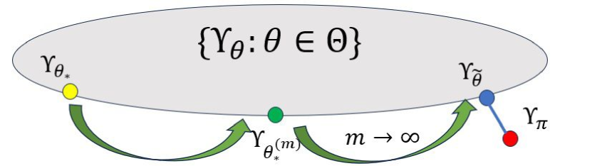
Figure 1: Larger $m$ makes $(\mathcal{T}^{\pi})^{m}\Upsilon_{\theta}\approx\Upsilon_{\pi}$ in expected energy distance, and thereby leads to $\theta_{*}^{(m)}\approx\tilde{\theta}$.

The above intuition is exemplified in the following simulated example, where the conditional distribution of a bivariate return is modeled by a Gaussian distribution known up to the correlation parameter $\theta\in[-1,1]$ with misspecified marginal variances (details in Appendix C.3.2). Figure 2 depicts the the true Bellman residual $F_{m}(\theta):=\bar{\mathcal{E}}(\Upsilon_{\theta},(\mathcal{T}^{\pi})^{m}\Upsilon_{\theta})$ with $m=1$, $100$ and $\infty$. This illustrates that $F_{m}$ uniformly converges to the inaccuracy function $F(\theta):=\bar{\mathcal{E}}(\Upsilon_{\theta},\Upsilon_{\pi})$ as indicated in (16), eventually leading to $\theta_{*}^{(m)}\rightarrow\tilde{\theta}$ as $m\rightarrow\infty$.

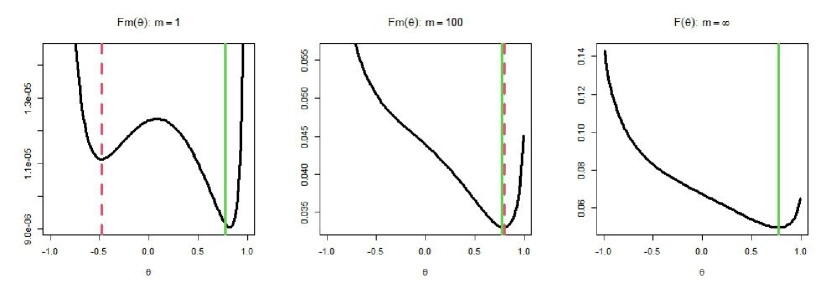
Figure 2: As $m\rightarrow\infty$, the selected minimizer (red) approximates $\tilde{\theta}$ (green) that corresponds to the best approximation (17), which is the closest to $\Upsilon_{\pi}$ among the candidates $\{\Upsilon_{\theta}:\theta\in\Theta\}$.

One can intuitively guess that larger step level $m$ is required when the extent of non-realizability is large. Although multi-step idea has been widely employed for the purpose of improving sample efficiency particularly in traditional RL [e.g., 4], ours is the first approach to use it in DRL for the purpose of overcoming non-realizability, to the best of our knowledge.

4.2 Bootstrap Operator

Generalizing from the definition of $\hat{\mathcal{T}}^{\pi}$ based on (9), we consider $\hat{Z}^{(m)}(s,a;\theta)\sim(\hat{\mathcal{T}}^{\pi})^{m}\Upsilon_{\theta}(s,a)$ as the distribution of an $m$-lengthed trajectories of tuples $(s,a,r,s^{\prime})$ that is generated under the estimated transition $\hat{p}$ and the target policy $\pi$:

$$\hat{Z}^{(m)}(s,a;\theta)\buildrel D\over{=}\sum_{t=1}^{m}\gamma^{t-1}\hat{R}^{(t)}+\gamma^{m}Z(\hat{S}^{(m)},\hat{A}^{(m)};\theta),$$ (18)

where $(\hat{R}^{(t)},\hat{S}^{(t)})\sim\hat{p}(\cdots|\hat{S}^{(t-1)},\hat{A}^{(t-1)})$, $\hat{A}^{(t)}\sim\pi(\cdot|\hat{S}^{(t)})$ for all $t\geq 1$, $(\hat{S}^{(0)},\hat{A}^{(0)})=(s,a)$. Now we can define the estimated and the population Bellman residual, as well as the inaccuracy function, along with their minimizers as:

$$\hat{F}_{m}(\theta):=\hat{\bar{\mathcal{E}}}\big{(}\Upsilon_{\theta},(\hat{\mathcal{T}}^{\pi})^{m}\Upsilon_{\theta}\big{)},\ \hat{\theta}^{(m)}:=\arg\min_{\theta\in\Theta}\hat{F}_{m}(\theta)$$

$$F_{m}(\theta):=\bar{\mathcal{E}}\big{(}\Upsilon_{\theta},(\mathcal{T}^{\pi})^{m}\Upsilon_{\theta}\big{)},\ \theta_{*}^{(m)}:=\arg\min_{\theta\in\Theta}F_{m}(\theta)$$

$$F(\theta):=\bar{\mathcal{E}}\big{(}\Upsilon_{\theta},\Upsilon_{\pi}\big{)},\ \tilde{\theta}:=\arg\min_{\theta\in\Theta}F(\theta).$$ (19)

However, the estimation of the $m$-step Bellman operator (18) generally requires the computation of $N^{m}$ trajectories (as discussed in Appendix B.1), which amounts to a heavy computational burden.

To alleviate such burden, we will instead bootstrap $M\ll N^{m}$ many trajectories by first sampling the initial state-action pairs $(s_{i}^{(0)},a_{i}^{(0)})\ (1\leq i\leq M)$ from $\hat{b}_{\mu}$ and then resampling the subsequent $r_{i}^{(t+1)},s_{i}^{(t+1)}\sim\hat{p}(\cdots|s_{i}^{(t)},a_{i}^{(t)})$ and $a_{i}^{(t+1)}\sim\pi(\cdot|s_{i}^{(t+1)})$ for $m$ steps. Let $\hat{p}_{m}^{(B)}(\cdots|s,a)$ be the empirical probability measure of $(\sum_{t=1}^{m}\gamma^{t-1}r_{i}^{(t)},s_{i}^{(m)})$ conditioning on $(s_{i}^{(0)},a_{i}^{(0)})=(s,a)$. We define the bootstrap operator as follows, with an abuse of notation $\mathcal{B}_{m}Z(s,a;\theta)\sim\mathcal{B}_{m}\Upsilon_{\theta}(s,a)$:

$$\mathcal{B}_{m}Z(s,a;\theta):=\sum_{t=1}^{m}\gamma^{t-1}\hat{R}_{b}^{(t)}+\gamma^{m}Z(\hat{S}_{b}^{(m)},\hat{A}_{b}^{(m)};\theta),$$ (20)

where we have $(\sum_{t=1}^{m}\gamma^{t-1}\hat{R}_{b}^{(t)},\hat{S}_{b}^{(m)})\sim\hat{p}_{m}^{(B)}(\cdots|s,a)$ and $\hat{A}_{b}^{(m)}\sim\pi(\cdot|\hat{S}_{b}^{(m)})$. Then we can compute our objective function and derive the bootstrap-based multi-step estimator:

$$\hat{F}_{m}^{(B)}(\theta):=\hat{\bar{\mathcal{E}}}\big{(}\Upsilon_{\theta},\mathcal{B}_{m}\Upsilon_{\theta}\big{)},\ \hat{\theta}_{m}^{(B)}:=\arg\min_{\theta\in\Theta}\hat{F}_{m}^{(B)}(\theta).$$ (21)

We will refer to this method as EBRM-multi-step, whose procedure is summarized in Algorithm 2.

Algorithm 2 EBRM-multi-step

Input: $\Theta$, $\mathcal{D}=\{(s_{i},a_{i},r_{i},s_{i}^{\prime})\}_{i=1}^{N}$, $m$, $M$

Output: $\hat{\theta}_{m}^{(B)}$

Estimate $\hat{b}_{\mu}$ and $\hat{p}$. $\triangleright$ Refer to Equation (9).

Randomly generate $M$ tuples of $(\sum_{t=1}^{m}\gamma^{t-1}r_{i}^{(t)},s_{i}^{(m)})\ (1\leq i\leq M)$.

$\hat{\theta}_{m}^{(B)}=\arg\min_{\theta\in\Theta}\hat{\bar{\mathcal{E}}}(\Upsilon_{\theta},\mathcal{B}_{m}\Upsilon_{\theta})$. $\triangleright$ Refer to Equations (20) and (21).

4.3 Statistical Error Bound

In this section, we develop a theoretical guarantee for $\bar{\mathcal{E}}\big{(}\Upsilon_{\hat{\theta}_{m}^{(B)}},\Upsilon_{\tilde{\theta}}\big{)}$, where $\Upsilon_{\tilde{\theta}}$ is the best approximation we can achieve under the non-realizability. To proceed, we first need to deal with the parameter convergence from $\hat{\theta}_{m}^{(B)}$ to $\tilde{\theta}$, which relies on the following assumptions regarding the candidate space $\Theta$ and the inaccuracy function $F(\cdot)$ (19).

Assumption 4.1.

The candidate space $\Theta\subset\mathbb{R}^{p}$ is compact. Furthermore, there exists $L>0$ such that

$$\mathbb{W}_{1,\infty}(\Upsilon_{\theta_{1}},\Upsilon_{\theta_{2}})\leq L\|\theta_{1}-\theta_{2}\|\quad\mbox{for}\quad\forall\theta_{1},\theta_{2}\in\Theta,$$

where $\mathbb{W}_{1,\infty}$ is the supremum-extended (3) Wasserstein-1 metric $\mathbb{W}_{1}$.

We can replace $\mathbb{W}_{1,\infty}$ of Assumption 4.1 with another metric, as long as it satisfies the properties mentioned in Appendix B.2. Lipschitz continuity is involved in bounding the entropy with respect to $\mathbb{W}_{1,\infty}$. (See Remark A.5.)

Assumption 4.2.

The inaccuracy function $F(\cdot):\Theta\subset\mathbb{R}^{p}\rightarrow\mathbb{R}$ (defined in (19)) is quadratically lower bounded at $\tilde{\theta}$.

This assumption is satisfied when the function $F(\cdot)$ is strongly convex. We give an example with Gaussian return that satisfies Assumption 4.2 in Appendix C.3.3. Assumption 4.2 implies the existence of $c_{2}>0$ such that $F(\theta)\geq F(\tilde{\theta})+c_{2}\cdot\|\theta-\tilde{\theta}\|^{2}$ for all $\theta\in\Theta$. This assumption is imposed to obtain the convergence rate of our estimator by adopting M-estimation theory (Chapter 5 of [22]). Also, a more detailed version of the finite-sample error bound for a fixed $m$ is given in Appendix B.5.3, which is in fact based on a weaker assumption (Assumption B.6).

Theorem 4.3.

Under Assumptions 2.1, 3.2, 4.1, 4.2, letting $M=\lfloor C_{1}\cdot N\rfloor$ and $m=\lfloor\frac{1}{4}\log_{(1/\gamma)}(C_{2}N/\log N)\rfloor$ for any positive constants $C_{1},C_{2}>0$, we have the following convergence rate of the upper bound

$$\bar{\mathcal{E}}\big{(}\Upsilon_{\hat{\theta}_{m}^{(B)}},\Upsilon_{\tilde{\theta}}\big{)}\leq\tilde{O}_{p}\bigg{[}\frac{1}{N^{1/8}}\cdot\bigg{\{}\log_{\frac{1}{\gamma}}\bigg{(}\frac{N}{\log N}\bigg{)}\bigg{\}}\bigg{]},$$

where $\tilde{O}_{p}$ indicates the rate of convergence up to logarithmic order.

The convergence rate of Theorem 4.3 is the result of the (asymptotically) optimal choice of $M$ and $m$. In our analysis, we notice a form of bias-variance trade-off in the selection of $m$, as explained in Appendix B.5.4. Practically, we set $M=N$ which works fine in the simulations of Section 5. A practical choice of $m$ is provided in Appendix D.3.1.

Note that the finite-sample error bound in Appendix B.5.3 is applicable to the setting with $m=1$ and realizability assumption. For instance, assuming that the inaccuracy function $F(\theta)$ is lower-bounded by a quadratic polynomial ($q=2$ in Assumption B.6, which corresponds to Assumption 4.2), it gives us the bound $O[\{\log(N/\delta)/N\}^{1/8}]$ under the ideal case where we can ignore the last two sources of inaccuracy specified in Appendix B.5.4, associated with bootstrap and non-realizability. We can see that it is much slower than the convergence rate $O(\sqrt{\log(N/\delta)/N})$ of Theorem 3.3, implying that it does not degenerate into Theorem 3.3. This is fundamentally due to a different proof structure that can be introduced via the application of Theorem 2.2 in the proof of Theorem 3.3. As explained earlier in Section 4.1, Theorem 2.2 can be used effectively to construct convergence of $\hat{\theta}$ under realizability. We provide a more detailed discussion for the rate mismatch in Appendix C.3.4.

5 Experiments

We assume a state space $\mathcal{S}=\{1,2,\cdots,30\}$ and an action space $\mathcal{A}=\{-1,1\}$, each action representing left or right. With the details of the environment in Appendix D.2.1, the initial state distribution and behavior / target policies are

$$S\sim\text{Unif}\big{\{}1,2,\cdots,30\big{\}}\quad\mbox{and}\quad A\sim b(\cdot|S),$$ (22)

$$b(a|s)=1/2\quad\mbox{and}\quad\pi(1|s)=1\quad\mbox{for}\quad\forall s,a\in\mathcal{S\times A}.$$

We compare three methods: EBRM, FLE [26], and QRTD [6]. Here, we assume realizability where the correct model is known (details in Appendix D.2.2) under two settings (with small and large variances), and the step level $m$ for EBRM is chosen in a data-adaptive way in Appendix D.3.1. With other tuning parameter selections explained in Appendix D.3, we repeated 100 simulations with the given sample size for each case, whose mean and standard deviation (within parenthesis) are recorded in Table 2. EBRM showed the lowest inaccuracy values measured by $\bar{\mathcal{E}}(\Upsilon_{\hat{\theta}},\Upsilon_{\pi})$, $\overline{\mathbb{W}}_{1}(\Upsilon_{\hat{\theta}},\Upsilon_{\pi})$, and $\mathbb{W}_{1}(\Upsilon_{\hat{\theta}}^{marginal},\Upsilon_{\pi}^{marginal})$, last of which was used by Wu [26] as an inaccuracy measure (see their Corollary 4.14). Here, $\overline{\mathbb{W}}_{1}$ is the expectation-extended Wasserstein-1 metric (5), and $\Upsilon^{marginal}\in\mathcal{P}(\mathbb{R}^{d})$ is defined as the mixture of $\{\Upsilon(s,a):s,a\in\mathcal{S\times A}\}$ with weights $\{b_{\mu}(s,a):s,a\in\mathcal{S\times A}\}$.

We also performed simulations in non-realizable scenarios (Appendix D.2.3) with more variety of sample sizes (Tables 8–13 of Appendix D.4). In most cases, EBRM showed outstanding performance.

Table 2: Mean $\bar{\mathcal{E}}$-inaccuracy (top), $\overline{\mathbb{W}}_{1}$-inaccuracy (middle), $\mathbb{W}_{1}$-inaccuracy (bottom) (standard deviation in parenthesis) over 100 simulations under realizability ($\gamma=0.99$). Smallest inaccuracy values are in boldface.

	Small variance			Large variance
Sample size	$2000$	$5000$	$10000$	$2000$	$5000$	$10000$
EBRM (Ours)	0.046	0.019	0.008	0.728	0.301	0.128
	(0.060)	(0.022)	(0.010)	(0.920)	(0.354)	(0.167)
FLE	5.533	2.385	1.220	24.603	14.482	6.528
	(6.448)	(2.883)	(1.618)	(25.768)	(16.101)	(7.814)
QRTD	48.679	46.032	49.402	105.274	75.173	70.483
	(34.323)	(30.909)	(34.617)	(11.728)	(21.515)	(33.965)

	Small variance			Large variance
Sample size	$2000$	$5000$	$10000$	$2000$	$5000$	$10000$
EBRM (Ours)	1.339	0.985	0.782	21.221	15.532	12.371
	(0.651)	(0.388)	(0.227)	(10.337)	(6.117)	(3.595)
FLE	12.374	8.036	5.694	101.232	79.628	53.745
	(7.843)	(5.091)	(3.773)	(58.586)	(46.772)	(33.948)
QRTD	56.739	54.397	57.145	274.405	236.383	223.537
	(23.716)	(22.259)	(24.314)	(11.003)	(22.376)	(38.935)

	Small variance			Large variance
Sample size	$2000$	$5000$	$10000$	$2000$	$5000$	$10000$
EBRM (Ours)	2.052	0.843	0.629	18.021	11.613	7.528
	(0.778)	(0.556)	(0.350)	(12.227)	(8.077)	(5.306)
FLE	12.328	8.013	5.596	94.556	71.430	46.740
	(7.859)	(5.113)	(3.786)	(62.630)	(51.205)	(36.986)
QRTD	47.738	45.764	49.851	247.308	198.257	191.908
	(25.251)	(25.656)	(27.463)	(16.843)	(29.911)	(48.057)

6 Conclusion

In this paper, we justify the use of expectation-extended distances for Bellman residual minimization in DRL under general state-action space (e.g. continuous), based on which we propose a distributional OPE method called EBRM. We establish its finite sample error bounds with or without realizability assumption, however focused on tabular case for deeper analysis. One interesting future direction is to extend EBRM towards non-tabular case via linear MDP [e.g., 9, 3], which we discussed in Appendix C.3.5.

Appendix A Proofs for Sections 2 and 3

A.1 Bounding Radon-Nikodym Derivative

Let $t\in\mathbb{N}$ be arbitrary. Then we have the following for all $s,a\in\mathcal{S\times A}$ by Assumption 2.1, with $\nu$ being the underlying measure of $\mathcal{S\times A}$,

$$\frac{q_{b_{\mu}}^{\pi:t}(s,a)}{b_{\mu}(s,a)}\leq\int_{\mathcal{S\times A}}q^{\pi}(s,a|\tilde{s},\tilde{a})\cdot q_{b_{\mu}}^{\pi:t-1}(\tilde{s},\tilde{a})\mathrm{d}\nu(\tilde{s},\tilde{a})\cdot\frac{1}{b_{\mu}(s,a)}\leq\sup_{\tilde{s},\tilde{a}}\sup_{s,a}\frac{q^{\pi}(s,a|\tilde{s},\tilde{a})}{b_{\mu}(s,a)}<\infty,$$

where $q_{b_{\mu}}^{\pi:0}=b_{\mu}$. Since $t\in\mathbb{N}$ was arbitrary, this implies existence of $C(t),C_{\rm sup}\in(0,\infty)$ such that

$$\sup_{s,a}\bigg{\{}\frac{q_{b_{\mu}}^{\pi:t}(s,a)}{b_{\mu}(s,a)}\bigg{\}}\leq C(t)\leq C_{{\rm sup}}<\infty\ \ \text{for }\forall\ t\in\mathbb{N}.$$ (23)

A.2 Proof of Theorem 2.2

A.2.1 Properties of Distance

Property 1.

$\eta$ satisfies translation-invariance and scale-sensitivity of order $\beta_{0}>0$. That is, with $z$ being an arbitrary (nonrandom) constant of computable size and $c\in\mathbb{R}$,

$$\eta\{\mathcal{L}(z+X),\mathcal{L}(z+Y)\}\leq\eta\{\mathcal{L}(X),\mathcal{L}(Y)\}\ \ \&\ \ \eta\{\mathcal{L}(cX),\mathcal{L}(cY)\}\leq|c|^{\beta_{0}}\eta\{\mathcal{L}(X),\mathcal{L}(Y)\}.$$

Property 2.

Letting $\mu(\cdot),\nu(\cdot):\mathcal{Z}\rightarrow\mathcal{P}(\mathbb{R}^{d})$ have different probability measures depending on the index random variable $Z\in\mathcal{Z}$ that follows a distribution $P(\cdot)$, the distance between probability-mixtures $\int_{\mathcal{Z}}\mu(z)\mathrm{d}P(z)$ and $\int_{\mathcal{Z}}\nu(z)\mathrm{d}P(z)$ satisfies convexity, that is

$$\eta\bigg{\{}\int_{\mathcal{Z}}\mu(z)\mathrm{d}P(z),\int_{\mathcal{Z}}\nu(z)\mathrm{d}P(z)\bigg{\}}\leq\int_{\mathcal{Z}}\eta\{\mu(z),\nu(z)\}\mathrm{d}P(z)=:\mathbb{E}_{Z\sim P}[\eta\{\mu(Z),\nu(Z)\}].$$

Property 3.

It satisfies the following Relaxed Triangular Inequality for all integers $K\geq 2$,

$$\eta(\mathcal{L}(X_{0}),\mathcal{L}(X_{K})) \leq K\sum_{i=0}^{K-1}\eta(\mathcal{L}(X_{i}),\mathcal{L}(X_{i+1})).$$ (24)

This is satisfied by all squared metric, that is $\eta(P,Q)=\rho^{2}(P,Q)$ for some probability metric $\rho$.

A.2.2 Proof

Let $\Upsilon\in\mathcal{P}(\mathbb{R}^{d})^{\mathcal{S\times A}}$ be arbitarily chosen. Starting with Relaxed Triangular Inequality (24) with $p=2$, we obtain the following for an arbitrary $t\in\mathbb{N}$,

$$\eta\bigg{\{}\Upsilon(s,a),\Upsilon_{\pi}(s,a)\bigg{\}} \leq 2\bigg{[}\underbrace{\eta\bigg{\{}\Upsilon(s,a),(\mathcal{T}^{\pi})^{t}\Upsilon(s,a)\bigg{\}}}_{(a)}+\underbrace{\eta\bigg{\{}(\mathcal{T}^{\pi})^{t}\Upsilon(s,a),\Upsilon_{\pi}(s,a)\bigg{\}}}_{(b)}\bigg{]}.$$ (25)

Let us first deal with $(b)$. Define $P_{t}^{\pi}(\cdots|s,a)$ to be the probability measure of the tuple $(\sum_{i=1}^{t}\gamma^{i-1}R^{(i)},S^{(t)},A^{(t)})$ after $t$ steps starting from the intial state-action pair $(S,A)=(s,a)$ under the given transition probability $(R^{(t)},S^{(t)})\sim p(\cdots|S^{(t-1)},A^{(t-1)})$ and the target policy $A^{(t)}\sim\pi(\cdot|S^{(t)})$. Further denoting the probability measure of $y+\gamma^{t}Z(s^{(t)},a^{(t)})$ with $Z(s,a)\sim\Upsilon(s,a)$ as $(g_{y,\gamma^{t}})_{\#}\Upsilon(s^{(t)},a^{(t)})$ for the fixed value of $s^{(t)},a^{(t)}$, $y=\sum_{i=1}^{t}\gamma^{i-1}r^{(i)}$ (which aligns with the notation $(g_{r,\gamma})_{\#}$ in (1)), we can obtain the following,

$$(b) =\eta\bigg{\{}(\mathcal{T}^{\pi})^{t}\Upsilon(s,a),(\mathcal{T}^{\pi})^{t}\Upsilon_{\pi}(s,a)\bigg{\}}\ \ \because(\mathcal{T}^{\pi})^{t}\Upsilon_{\pi}(s,a)=\Upsilon_{\pi}(s,a)$$

$$=\eta\bigg{\{}\int(g_{y,\gamma^{t}})_{\#}\Upsilon(s^{(t)},a^{(t)})\mathrm{d}P_{t}^{\pi}(y,s^{(t)},a^{(t)}|s,a),\int(g_{y,\gamma^{t}})_{\#}\Upsilon_{\pi}(s^{(t)},a^{(t)})\mathrm{d}P_{t}^{\pi}(y,s^{(t)},a^{(t)}|s,a)\bigg{\}}$$

$$\leq\int\eta\big{\{}(g_{y,\gamma^{t}})_{\#}\Upsilon(s^{(t)},a^{(t)}),(g_{y,\gamma^{t}})_{\#}\Upsilon_{\pi}(s^{(t)},a^{(t)})\big{\}}\mathrm{d}P_{t}^{\pi}(y,s^{(t)},a^{(t)}|s,a)\ \ \text{by Property \ref{mixture_inequality}}$$

$$\leq\int\gamma^{t\beta_{0}}\eta\bigg{\{}\Upsilon(s^{(t)},a^{(t)}),\Upsilon_{\pi}(s^{(t)},a^{(t)})\bigg{\}}\mathrm{d}P_{t}^{\pi}(s^{(t)},a^{(t)}|s,a)\ \ \text{by Property }\ref{translation_scale_sensitivity}$$

$$=\gamma^{t\beta_{0}}\mathbb{E}_{\pi}\bigg{[}\eta\bigg{\{}\Upsilon(S^{(t)},A^{(t)}),\Upsilon_{\pi}(S^{(t)},A^{(t)})\bigg{\}}\bigg{|}S=s,A=a\bigg{]}.$$ (26)

From now on, we will use $\mathbb{E}_{b_{\mu}}$ and $\mathbb{E}_{q_{b_{\mu}}^{\pi:t}}$ to denote the expectation with respect to the probability $(S,A)\sim b_{\mu}$ and $(S,A)\sim q_{b_{\mu}}^{\pi:t}$. Treating $(S,A)$ in Inequality (25) as random, we can obtain the following based on Inequality (A.2.2),

$$\mathbb{E}_{b_{\mu}}\bigg{[}(b)\bigg{]} \leq\gamma^{t\beta_{0}}\mathbb{E}\bigg{[}\eta\bigg{\{}\Upsilon(S^{(t)},A^{(t)}),\Upsilon_{\pi}(S^{(t)},A^{(t)}))\bigg{\}}\bigg{|}(S,A)\sim b_{\mu},\ A^{(i)}\sim\pi(\cdot|S^{(i)})\ \forall i\geq 1\bigg{]}$$

$$=\gamma^{t\beta_{0}}\mathbb{E}_{b_{\mu}}\bigg{[}\mathbb{E}_{\pi}\bigg{\{}\eta\bigg{(}\Upsilon(S^{(t)},A^{(t)}),\Upsilon_{\pi}(S^{(t)},A^{(t)})\bigg{)}\bigg{|}S,A\bigg{\}}\bigg{]}$$

$$=\gamma^{t\beta_{0}}\mathbb{E}_{q_{b_{\mu}}^{\pi:t}}\bigg{[}\eta\bigg{\{}\Upsilon(S,A),\Upsilon_{\pi}(S,A)\bigg{\}}\bigg{]}\ \ \text{by definition of }q_{b_{\mu}}^{\pi:t}\ \text{under Assumption \ref{RN_derivative}}$$

$$=\gamma^{t\beta_{0}}\mathbb{E}_{b_{\mu}}\bigg{[}\eta\bigg{\{}\Upsilon(S,A),\Upsilon_{\pi}(S,A)\bigg{\}}\cdot\frac{q_{b_{\mu}}^{\pi:t}(S,A)}{b_{\mu}(S,A)}\bigg{]}$$

$$\leq C(t)\cdot\gamma^{t\beta_{0}}\cdot\bar{\eta}(\Upsilon,\Upsilon_{\pi})\ \ \text{by Inequality (\ref{Ct_and_Csup})}.$$ (27)

Now let us deal with $(a)$ of Inequality (25) using Property 3. Let $\Upsilon_{k}(s,a)=(\mathcal{T}^{\pi})^{k}\Upsilon(s,a)$. For sufficiently large $t\in\mathbb{N}$, we obtain the following by relaxed triangle inequality (24) with $K=2$,

$$\eta(\Upsilon (s,a),(\mathcal{T}^{\pi})^{t}\Upsilon(s,a))\leq 2\cdot\bigg{\{}\eta(\Upsilon_{0}(s,a),\Upsilon_{1}(s,a))+\eta(\Upsilon_{1}(s,a),\Upsilon_{t}(s,a))\bigg{\}}$$

$$\leq 2\cdot\eta(\Upsilon_{0}(s,a),\Upsilon_{1}(s,a))+2\cdot 2\cdot\bigg{\{}\eta(\Upsilon_{1}(s,a),\Upsilon_{3}(s,a))+\eta(\Upsilon_{3}(s,a),\Upsilon_{t}(s,a))\bigg{\}}$$

$$\leq 2\cdot\eta(\Upsilon_{0}(s,a),\Upsilon_{1}(s,a))+2^{2}\cdot\eta(\Upsilon_{1}(s,a),\Upsilon_{3}(s,a))$$

$$\qquad+2^{2}\cdot 2\cdot\bigg{\{}\eta(\Upsilon_{3}(s,a),\Upsilon_{7}(s,a))+\eta(\Upsilon_{7}(s,a),\Upsilon_{t}(s,a))\bigg{\}}$$

$$\leq 2\cdot\eta(\Upsilon_{0}(s,a),\Upsilon_{1}(s,a))+2^{2}\cdot\eta(\Upsilon_{1}(s,a),\Upsilon_{3}(s,a))+2^{3}\cdot\eta(\Upsilon_{3}(s,a),\Upsilon_{7}(s,a))+\cdots.$$

This can be further bounded as follows by relaxed triangle inequality (24), this time with general $K\geq 2$,

$$\eta(\Upsilon(s,a), (\mathcal{T}^{\pi})^{t}\Upsilon(s,a))\leq 2\cdot\eta(\Upsilon_{0}(s,a),\Upsilon_{1}(s,a))$$

$$\ \ +2^{2}\cdot 2\cdot\big{\{}\eta(\Upsilon_{1}(s,a),\Upsilon_{2}(s,a))+\eta(\Upsilon_{2}(s,a),\Upsilon_{3}(s,a))\big{\}}$$

$$\ \ +2^{3}\cdot 2^{2}\cdot\big{\{}\eta(\Upsilon_{3}(s,a),\Upsilon_{4}(s,a))+\cdots+\eta(\Upsilon_{6}(s,a),\Upsilon_{7}(s,a))\big{\}}+\cdots,$$

which can finally be formalized into

$$(a) \leq\sum_{k=1}^{\infty}2^{2k-1}\cdot\sum_{j=0}^{s_{1}(k)}\eta\bigg{(}\Upsilon_{s_{1}(k)+j}(s,a),\Upsilon_{s_{1}(k)+j+1}(s,a)\bigg{)}\ \ \text{where }s_{1}(k)=2^{k-1}-1.$$

Therefore we can further obtain following using similar logic as Inequality (A.2.2),

$$\mathbb{E}_{b_{\mu}}\bigg{[}(a)\bigg{]}\leq\sum_{k=1}^{\infty}2^{2k-1}\cdot\sum_{j=0}^{s_{1}(k)}\mathbb{E}_{b_{\mu}}\bigg{[}\eta\bigg{\{}\Upsilon_{s_{1}(k)+j}(S,A),\Upsilon_{s_{1}(k)+j+1}(S,A)\bigg{\}}\bigg{]}$$

$$\leq\sum_{k=1}^{\infty}2^{2k-1}\cdot\sum_{j=0}^{s_{1}(k)}\mathbb{E}_{b_{\mu}}\bigg{[}\eta\bigg{\{}(\mathcal{T}^{\pi})^{s_{1}(k)+j}\Upsilon(S,A),(\mathcal{T}^{\pi})^{s_{1}(k)+j+1}\Upsilon(S,A)\bigg{\}}\bigg{]}$$

$$\leq\sum_{k=1}^{\infty}2^{2k-1}\cdot\sum_{j=0}^{s_{1}(k)}\gamma^{(s_{1}(k)+j)\beta_{0}}\cdot\mathbb{E}_{q_{b_{\mu}}^{\pi:s_{1}(k)+j}}\bigg{[}\eta\bigg{\{}\Upsilon(S,A),\mathcal{T}^{\pi}\Upsilon(S,A)\bigg{\}}\bigg{]}$$

$$\leq\sum_{k=1}^{\infty}2^{2k-1}\cdot\sum_{j=0}^{s_{1}(k)}\gamma^{(s_{1}(k)+j)\beta_{0}}\cdot C(s_{1}(k)+j)\cdot\mathbb{E}_{b_{\mu}}\bigg{[}\eta\bigg{\{}\Upsilon(S,A),\mathcal{T}^{\pi}\Upsilon(S,A)\bigg{\}}\bigg{]}$$

$$=\sum_{k=1}^{\infty}2^{2k-1}\cdot\sum_{j=0}^{2^{k-1}-1}\gamma^{(2^{k-1}-1+j)\beta_{0}}\cdot C(2^{k-1}-1+j)\cdot\mathbb{E}_{b_{\mu}}\bigg{[}\eta\bigg{\{}\Upsilon(S,A),\mathcal{T}^{\pi}\Upsilon(S,A)\bigg{\}}\bigg{]}.$$ (28)

Note that we have

$$B(\gamma;\beta_{0}) :=\sum_{k=1}^{\infty}2^{2k-1}\cdot\sum_{j=0}^{2^{k-1}-1}\gamma^{(2^{k-1}-1+j)\beta_{0}}=\sum_{k=1}^{\infty}2^{2k-1}\cdot\gamma^{(2^{k-1}-1)\beta_{0}}\cdot\sum_{j=0}^{2^{k-1}-1}(\gamma^{\beta_{0}})^{j}$$

$$\leq\bigg{(}\sum_{k=1}^{\infty}2^{2k-1}\cdot\gamma^{(2^{k-1}-1)\beta_{0}}\bigg{)}\cdot\bigg{(}\sum_{j=0}^{\infty}\gamma^{\beta_{0}\cdot j}\bigg{)}\leq\frac{1}{2(1-\gamma^{\beta_{0}})}\sum_{k=1}^{\infty}(4^{k}\cdot\gamma^{(2^{k-1}-1)\beta_{0}})<\infty,$$

and Inequalities (A.2.2) and (A.2.2) can thereby be switched into the following bound, since $C(t)\leq C_{{\rm sup}}$ by Inequality (23),

$$\mathbb{E}_{b_{\mu}}\bigg{[}(a)\bigg{]}\leq C_{{\rm sup}}\cdot B(\gamma;\beta_{0})\cdot\bar{\eta}(\Upsilon,\mathcal{T}^{\pi}\Upsilon)\quad\&\quad\mathbb{E}_{b_{\mu}}\bigg{[}(b)\bigg{]}\leq C_{{\rm sup}}\cdot\gamma^{t\beta_{0}}\bar{\eta}(\Upsilon,\Upsilon_{\pi}).$$

Then starting from Inequality (25), we can obtain

$$\bar{\eta}(\Upsilon,\Upsilon_{\pi}) \leq 2\cdot\bigg{\{}\mathbb{E}_{b_{\mu}}\bigg{[}(a)\bigg{]}+\mathbb{E}_{b_{\mu}}\bigg{[}(b)\bigg{]}\bigg{\}}\leq 2C_{{\rm sup}}\cdot\bigg{\{}B(\gamma;\beta_{0})\cdot\bar{\eta}(\Upsilon,\mathcal{T}^{\pi}\Upsilon)+\gamma^{t\beta_{0}}\bar{\eta}(\Upsilon,\Upsilon_{\pi})\bigg{\}}.$$

Letting $t\rightarrow\infty$ and replacing $B(\gamma;\beta_{0})$ with $B_{1}(\gamma;\beta_{0}):=\frac{1}{2(1-\gamma^{\beta_{0}})}\sum_{k=1}^{\infty}(4^{k}\cdot\gamma^{(2^{k-1}-1)\beta_{0}})$, we obtain

$$\bar{\eta}(\Upsilon,\Upsilon_{\pi})\leq 2C_{{\rm sup}}B_{1}(\gamma;\beta_{0})\cdot\bar{\eta}(\Upsilon,\mathcal{T}^{\pi}\Upsilon),$$ (29)

where $C_{\rm sup}$ is defined in (23). This yields Theorem 2.2.

A.3 Proof that Energy Distance satisfies Properties A.2.1

Property 1 is straightforward from the definition of Energy Distance (7). For an arbitrary $\mathbf{c}\in\mathbb{R}^{d}$ and $c\in\mathbb{R}$, we have the following that leads to $\beta_{0}=1$ in Property 1,

$$\mathcal{E}\big{\{}\mathcal{L}(\mathbf{c}+\mathbf{X}),\mathcal{L}(\mathbf{c}+\mathbf{Y})\big{\}}=\mathcal{E}\big{\{}\mathcal{L}(\mathbf{X}),\mathcal{L}(\mathbf{Y})\big{\}}\quad\&\quad\mathcal{E}\big{\{}\mathcal{L}(c\mathbf{X}),\mathcal{L}(c\mathbf{Y})\big{\}}=|c|\cdot\mathcal{E}\big{\{}\mathcal{L}(\mathbf{X}),\mathcal{L}(\mathbf{Y})\big{\}}.$$

Property 2 is shown by Nguyen (Lemma 3 of [15]).

Property 3 can be verified as follows. Since $\mathcal{E}$ is a squared $\mathrm{MMD}_{k}$ corresponding to the kernel $k(\mathbf{x},\mathbf{y})=\|\mathbf{x}\|+\|\mathbf{y}\|-\|\mathbf{x}-\mathbf{y}\|$, it is a squared form of some metric $\rho$ between two distributions $P,Q$ by Gretton (Lemma 4 of [7]),

$$\mathcal{E}(P,Q)=\rho^{2}(P,Q)\ \ \text{where}\ \ \rho(P,Q):=\|\mu_{P}-\mu_{Q}\|_{\mathcal{H}}$$

where $\mu_{P},\mu_{Q}\in\mathcal{H}$ are the mean embeddings of $P,Q$, and $\mathcal{H}$ is the RKHS corresponding to the suggested kernel $k$. Based on this, we can derive the so-called Relaxed Triangular Inequality,

$$\mathcal{E}(\mathcal{L}(X_{0}),\mathcal{L}(X_{K})) =\rho^{2}(\mathcal{L}(X_{0}),\mathcal{L}(X_{K}))\leq\bigg{\{}\sum_{i=0}^{K-1}\rho(\mathcal{L}(X_{i}),\mathcal{L}(X_{i+1}))\bigg{\}}^{2}$$

$$\leq K\sum_{i=0}^{K-1}\mathcal{E}(\mathcal{L}(X_{i}),\mathcal{L}(X_{i+1})),$$

where the inequality of the second line used $ab+ba\leq a^{2}+b^{2}$ that leads to $(a_{1}+\cdots+a_{K})^{2}\leq K\cdot(a_{1}^{2}+\cdots+a_{K}^{2})$. Plugging in $K=2$ gives us the following special case,

$$\mathcal{E}\{\mathcal{L}(X_{0}),\mathcal{L}(X_{2})\}\leq 2\cdot[\mathcal{E}\{\mathcal{L}(X_{0}),\mathcal{L}(X_{1})\}+\mathcal{E}\{\mathcal{L}(X_{1}),\mathcal{L}(X_{2})\}].$$ (30)

A.4 Explanation of sub-Gaussian norm

Sub-Gaussianity can be quantified with sub-Gaussian norm $\|\cdot\|_{\psi_{2}}:\mathcal{P}(\mathbb{R})\rightarrow\mathbb{R}\ \text{or }\mathcal{P}(\mathbb{R}^{d})\rightarrow\mathbb{R}$ (Definitions 2.5.6 and 3.4.1 by [23],

$$\|X\|_{\psi_{2}}:=\inf\bigg{\{}t>0:\ \mathbb{E}(X^{2}/t^{2})\leq 2\bigg{\}}\ (d=1)\quad\&\quad\|\mathbf{X}\|_{\psi_{2}}:=\sup_{\mathbf{x}\in\mathbb{R}^{d}:\|\mathbf{x}\|=1}\|\langle\mathbf{X},\mathbf{x}\rangle\|_{\psi_{2}}.$$ (31)

Sub-Gaussian norm is verified to be a valid norm in Exercise 2.5.7 suggested by Vershynin [23]. Random variable (vector) $\mathbf{X}$ is called sub-Gaussian if it satisfies $\|\mathbf{X}\|_{\psi_{2}}<\infty$. A lot of useful inequalilties, such as Dudley’s integral inequality and and Hoeffding’s inequality (Theorems C.1, C.2) are based on sub-Gaussianity assumption.

A.5 Bounding expectation-difference with Wasserstein-1 metric

Let $c\in\mathbb{R}^{d}$, $\gamma_{1},\gamma_{2}\in[0,1]$, and $(s,a),(\tilde{s},\tilde{a})\in\mathcal{S\times A}$ be arbitrary, $Z_{i}(s,a)\sim\Upsilon_{i}(s,a)$ with $Z_{1}(s,a)$, $Z_{2}(\tilde{s},\tilde{a})$ and $Z_{3}(s,a)$, $Z_{4}(\tilde{s},\tilde{a})$ being pairwise independent. Letting $J_{13}$ be the possible dependence structures (or joint distributions) between marginal distributions of $Z_{1}(s,a)$ and $Z_{2}(s,a)$, and $J_{24}$ be that between $Z_{3}(\tilde{s},\tilde{a})$ and $Z_{4}(\tilde{s},\tilde{a})$, we have

$$\bigg{|}\mathbb{E}\|c+\gamma_{1} Z_{1}(s,a)-\gamma_{2}Z_{2}(\tilde{s},\tilde{a})\|-\mathbb{E}\|c+\gamma_{1}Z_{3}(s,a)-\gamma_{2}Z_{4}(\tilde{s},\tilde{a})\|\bigg{|}$$

$$=\inf_{J_{13},J_{24}}\bigg{|}\mathbb{E}\|c+\gamma_{1}Z_{1}(s,a)-\gamma_{2}Z_{2}(\tilde{s},\tilde{a})\|-\mathbb{E}\|c+\gamma_{1}Z_{3}(s,a)-\gamma_{2}Z_{4}(\tilde{s},\tilde{a})\|\bigg{|}$$

$$\leq\inf_{J_{13},J_{24}}\mathbb{E}\|c+\gamma_{1}Z_{1}(s,a)-\gamma_{2}Z_{2}(\tilde{s},\tilde{a})-c-\gamma_{1}Z_{3}(s,a)+\gamma_{2}Z_{4}(\tilde{s},\tilde{a})\|$$

$$=\inf_{J_{13}}\mathbb{E}\|\gamma_{1}Z_{1}(s,a)-\gamma_{1}Z_{3}(s,a)\|+\inf_{J_{24}}\mathbb{E}\|\gamma_{2}Z_{2}(\tilde{s},\tilde{a})-\gamma_{2}Z_{4}(\tilde{s},\tilde{a})\|$$

$$=\gamma_{1}\cdot\mathbb{W}_{1}(Z_{1}(s,a),Z_{3}(s,a))+\gamma_{2}\cdot\mathbb{W}_{1}(Z_{2}(s,a),Z_{4}(s,a))$$

$$\leq\gamma_{1}\cdot\mathbb{W}_{1,\infty}(\Upsilon_{1},\Upsilon_{3})+\gamma_{2}\cdot\mathbb{W}_{1,\infty}(\Upsilon_{2},\Upsilon_{4}),$$

where the second last line holds by the definition of Wasserstein-1 metric.

A.6 Proof of Theorem 3.3

Throughout the proof, we will use $C>0$, $C_{k}>0$ ($k\in\mathbb{N}$) to denote appropriate universal constants.

In addition, we define the minimizer of Bellman residual $\theta_{*}:\in\arg\min_{\theta\in\Theta}\bar{\mathcal{E}}(\Upsilon_{\theta},\mathcal{T}^{\pi}\Upsilon_{\theta})$. Since $\Upsilon_{\pi}=\Upsilon_{\theta^{\prime}}$ for some $\theta^{\prime}\in\Theta$ by Assumption 3.1, we have $\bar{\mathcal{E}}(\Upsilon_{\theta^{\prime}},\mathcal{T}^{\pi}\Upsilon_{\theta^{\prime}})=\bar{\mathcal{E}}(\Upsilon_{\pi},\mathcal{T}^{\pi}\Upsilon_{\pi})=0$, thereby becoming the minimizer of Bellman residual. Then we can let $\theta_{*}=\theta^{\prime}$, and have $\bar{\mathcal{E}}(\Upsilon_{\theta_{*}},\mathcal{T}^{\pi}\Upsilon_{\theta_{*}})=0$, that is $\Upsilon_{\theta_{*}}=\mathcal{T}^{\pi}\Upsilon_{\theta_{*}}$.

Lastly, we would like to allow abuse of notation $\mathbb{W}_{1,\infty}(\theta_{1},\theta_{2}):=\mathbb{W}_{1,\infty}(\Upsilon_{\theta_{1}},\Upsilon_{\theta_{2}})$, with which we will define the diameter ${\rm diam}(\Theta;\mathbb{W}_{1,\infty}):=\sup_{\theta_{1},\theta_{2}\in\Theta}\{\mathbb{W}_{1,\infty}(\theta_{1},\theta_{2})\}$. Based on the metric $\mathbb{W}_{1,\infty}$, we will quantify the model complexity with covering number (Definition 4.2.2 by [23]). With $N_{\mathbb{W}_{1,\infty}}(\theta,t):=\{\theta^{\prime}\in\Theta:\mathbb{W}_{1,\infty}(\theta^{\prime},\theta)<t\}$ being $t$-neighborhood of $\theta\in\Theta$, we define the covering number as $\mathcal{N}(\Theta,\mathbb{W}_{1,\infty},t):=\min\{\tilde{M}\in\mathbb{N}:\exists\theta_{1},\cdots,\theta_{\tilde{M}}\ \text{s.t. }\Theta\subset\cup_{i=1}^{\tilde{M}}N_{\mathbb{W}_{1,\infty}}(\theta_{i},t)\}$.

However, note that $\mathbb{W}_{1,\infty}$ in the previous paragraph can be replaced with a general distance measure $\tilde{\eta}$, as long as it satisfies the first two properties suggested in Appendix B.2.

A.6.1 Decomposition into Two Discrepancies

Defining $\Gamma_{N}$ and $\Delta_{N}$ as

$$\Gamma_{N}:=\sup_{\theta\in\Theta}\bar{\mathcal{E}}(\mathcal{T}^{\pi}\Upsilon_{\theta},\hat{\mathcal{T}}^{\pi}\Upsilon_{\theta})\ \ \&\ \ \Delta_{N}:=\sup_{\theta\in\Theta}\bigg{|}\bar{\mathcal{E}}(\Upsilon_{\theta},\hat{\mathcal{T}}^{\pi}\Upsilon_{\theta})-\hat{\bar{\mathcal{E}}}(\Upsilon_{\theta},\hat{\mathcal{T}}^{\pi}\Upsilon_{\theta})\bigg{|},$$

we can decompose the term $\bar{\mathcal{E}}(\Upsilon_{\hat{\theta}},\mathcal{T}^{\pi}\Upsilon_{\hat{\theta}})$ as follows.

$$\bar{\mathcal{E}}(\Upsilon_{\hat{\theta}},\mathcal{T}^{\pi}\Upsilon_{\hat{\theta}}) \leq 2\cdot\bigg{\{}\bar{\mathcal{E}}(\Upsilon_{\hat{\theta}},\hat{\mathcal{T}}^{\pi}\Upsilon_{\hat{\theta}})+\bar{\mathcal{E}}(\hat{\mathcal{T}}^{\pi}\Upsilon_{\hat{\theta}},\mathcal{T}^{\pi}\Upsilon_{\hat{\theta}})\bigg{\}}$$

$$\leq 2\cdot\bigg{\{}\hat{\bar{\mathcal{E}}}(\Upsilon_{\hat{\theta}},\hat{\mathcal{T}}^{\pi}\Upsilon_{\hat{\theta}})+\bigg{|}\hat{\bar{\mathcal{E}}}(\Upsilon_{\hat{\theta}},\hat{\mathcal{T}}^{\pi}\Upsilon_{\hat{\theta}})-\bar{\mathcal{E}}(\Upsilon_{\hat{\theta}},\hat{\mathcal{T}}^{\pi}\Upsilon_{\hat{\theta}})\bigg{|}+\bar{\mathcal{E}}(\hat{\mathcal{T}}^{\pi}\Upsilon_{\hat{\theta}},\mathcal{T}^{\pi}\Upsilon_{\hat{\theta}})\bigg{\}}$$

$$\leq 2\cdot\bigg{\{}\hat{\bar{\mathcal{E}}}(\Upsilon_{\theta_{*}},\hat{\mathcal{T}}^{\pi}\Upsilon_{\theta_{*}})+\Delta_{N}+\Gamma_{N}\bigg{\}}$$

$$\leq 2\cdot\bigg{\{}\bar{\mathcal{E}}(\Upsilon_{\theta_{*}},\hat{\mathcal{T}}^{\pi}\Upsilon_{\theta_{*}})+\bigg{|}\hat{\bar{\mathcal{E}}}(\Upsilon_{\theta_{*}},\hat{\mathcal{T}}^{\pi}\Upsilon_{\theta_{*}})-\bar{\mathcal{E}}(\Upsilon_{\theta_{*}},\hat{\mathcal{T}}^{\pi}\Upsilon_{\theta_{*}})\bigg{|}+\Delta_{N}+\Gamma_{N}\bigg{\}}$$

$$\leq 2\cdot\bigg{\{}\bar{\mathcal{E}}(\mathcal{T}^{\pi}\Upsilon_{\theta_{*}},\hat{\mathcal{T}}^{\pi}\Upsilon_{\theta_{*}})+2\Gamma_{N}+\Delta_{N}\bigg{\}}$$

$$\leq 4\cdot(\Gamma_{N}+\Delta_{N}).$$

Combined with the result (29) of Theorem 2.2 that requires Assumption 2.1, it leads to the following bound,

$$\bar{\mathcal{E}}(\Upsilon_{\hat{\theta}},\Upsilon_{\pi})\leq 8C_{{\rm sup}}B_{1}(\gamma)\cdot(\Gamma_{N}+\Delta_{N}),\quad\mbox{where}$$ (32)

$$B_{1}(\gamma):=B_{1}(\gamma;1)=\frac{1}{2(1-\gamma)}\sum_{k=1}^{\infty}4^{k}\gamma^{2^{k-1}-1}\quad\mbox{by definition above \eqref{Fundamental_Realizable_specific}}$$

since we have verified $\beta_{0}=1$ in A.3. Now it suffices to bound $\Gamma_{N}$ and $\Delta_{N}$, which will be referred to as Bellman discrepancy and state-action discrepancy to indicate the sources of error, $\mathcal{T}^{\pi}$ and $b_{\mu}(s,a)$, respectively. Before we proceed, we list several properties of sub-Gaussian norm (31) that we will utilize in our analysis. Corresponding proofs can be found in Section C.2.1.

Remark A.1.

(Properties of sub-Gaussian norm) We have the following properties regarding sub-Gaussian norm,

1. For $X\sim Ber(p)$, we have $\|X\|_{\psi_{2}}\leq 1/\sqrt{\log 2}$.

2. For a constant $c\in\mathbb{R}$, $\|c\|_{\psi_{2}}=c/\sqrt{\log 2}$.

3. For a random variable $X\in\mathbb{R}$, $\|\mathbb{E}(X)\|_{\psi_{2}}\leq\|X\|_{\psi_{2}}$ holds.

4. For a random vector $\mathbf{X}\in\mathbb{R}^{d}$, $\big{\|}\|\mathbf{X}\|\big{\|}_{\psi_{2}}\leq d\big{\|}\mathbf{X}\big{\|}_{\psi_{2}}$ holds.

5. For a random variable $X\in\mathbb{R}$, $\|X-\mathbb{E}(X)\|_{\psi_{2}}\leq C\|X\|_{\psi_{2}}$ holds.

6. For iid mean-zero random variables $X_{1},\cdots,X_{n}$, we have $\|\frac{1}{n}\sum_{i=1}^{n}X_{i}\|_{\psi_{2}}\leq\frac{C}{\sqrt{n}}\cdot\|X_{1}\|_{\psi_{2}}.$

A.6.2 Conditioning on Sufficient Sample size for each state-action pair

Prior to bounding $\Gamma_{N}$ and $\Delta_{N}$ of (32), we will first condition upon an event where each state-action pair is observed sufficiently many times.

Before we proceed, we should note that the given probability space $(\Omega,\Sigma,\mathbb{P})$ can be factorized into two stages. Letting $\mathbf{N}=(N(s,a))_{s,a\in\mathcal{S\times A}}\in\mathbb{R}^{\mathcal{S\times A}}$ to be a random vector that indicates the observed number of samples for each state-action pair, we can see that $(\Omega,\Sigma,\mathbb{P})$ consists of two consecutive probability events denoted as follows,

Stage 1: $$\ (\Omega_{\mathcal{S\times A}},\Sigma_{\mathcal{S\times A}},\mathbb{P}_{\mathcal{S\times A}})\Rightarrow\text{determines sampling of state-action pairs }S_{i},A_{i}\sim b_{\mu},$$ (33)

Stage 2: $$\ (\Omega^{(\mathbf{N})},\Sigma^{(\mathbf{N})},\mathbb{P}^{(\mathbf{N})})\Rightarrow\text{conditioned on }(S_{i},A_{i}),\text{ determines }R_{i},S_{i}^{\prime}\sim p(\cdots|S_{i},A_{i}).$$

This implies that having sufficiently many observations for each $s,a$ is solely associated with probability space of Stage 1. Now let us discuss how “sufficiently large” $N(s,a)$ is characterized (35).

Temporarily assuming $N\geq 2$, we can divide the data $\mathcal{D}=\{(S_{i},A_{i},R_{i},S_{i}^{\prime})\}_{i=1}^{N}$ into two halves,

$$\mathcal{D}_{1}=\{(S_{i},A_{i},R_{i},S_{i}^{\prime})\}_{i=1}^{\lfloor N/2\rfloor}\quad\mbox{and}\quad\mathcal{D}_{2}=\{(S_{i},A_{i},R_{i},S_{i}^{\prime})\}_{i=\lfloor N/2\rfloor+1}^{N}.$$

Note that we denoted observations $(S_{i},A_{i},R_{i},S_{i}^{\prime})$ in capital letters, so as to indicate that they are random objects. Based on this, we define the following notations based on (9),

$$\mathbf{p}=\big{(}b_{\mu}(s,a)\big{)}_{s,a\in\mathcal{S\times A}}\in[0,1]^{\mathcal{S\times A}}\ \ \&\ \ \hat{\mathbf{p}}=\big{(}\hat{b}_{\mu}(s,a)\big{)}_{s,a\in\mathcal{S\times A}}\in[0,1]^{\mathcal{S\times A}},$$

and it is straightforward to see $\hat{\mathbf{p}}=\lfloor N/2\rfloor/N\cdot\hat{\mathbf{p}}_{(1)}+(N-\lfloor N/2\rfloor)/N\cdot\hat{\mathbf{p}}_{(2)}$, where each term in the RHS is sample mean based on $\mathcal{D}_{1}$ and $\mathcal{D}_{2}$,

$$\hat{\mathbf{p}}_{(1)}=\frac{1}{N/2}\sum_{i=1}^{N/2}\mathbf{y}_{i}\quad\mbox{and}\quad\hat{\mathbf{p}}_{(2)}=\frac{1}{N-\lfloor N/2\rfloor}\sum_{i=1}^{N-\lfloor N/2\rfloor}\mathbf{y}_{i},$$ (34)

with $\mathbf{y}_{i}\in\{0,1\}^{\mathcal{S\times A}}$ being indicators having 1 only at the state-action pair that $(S_{i},A_{i})$ correspond to. Within Stage 1 probability space (33), we define the following subset with given $\epsilon\in(0,1]$,

$$\Omega_{\mathcal{S\times A}}^{(\epsilon)}:=\bigg{\{}\omega\in\Omega_{\mathcal{S\times A}}\ \bigg{|}\ \|\hat{\mathbf{p}}_{(1)}-\mathbf{p}\|<\frac{1}{2}p_{{\rm min}}\cdot\epsilon\quad\mbox{and}\quad\|\hat{\mathbf{p}}_{(2)}-\mathbf{p}\|<\frac{1}{2}p_{{\rm min}}\cdot\epsilon\bigg{\}},$$ (35)

under which we can verify that following holds (proofs in C.2.2),

Fact 1: $$\hat{b}_{\mu}(s,a)=\frac{N(s,a)}{N}\in\bigg{[}\frac{1}{2}b_{\mu}(s,a),\frac{3}{2}b_{\mu}(s,a)\bigg{]}\text{ for }\forall s,a\in\mathcal{S\times A},$$ (36)

Fact 2: $$N(s,a)\geq 2\text{ for }\forall s,a\in\mathcal{S\times A},$$

Fact 3: $$\|\hat{\mathbf{p}}-\mathbf{p}\|<\frac{1}{2}p_{{\rm min}}\cdot\epsilon.$$

There is one fact which is crucially important about (35). The conditioned event of observing a plenty of samples for each $s,a$ (35) is not related at all with Stage 2 probability space (33). This implies that regardless of realizations of $\mathbf{N}$, the dependence structure between different samples (conditioned on the same $s,a$) $(R,S^{\prime})\sim p(\cdots|s,a)$ remains intact, i.e. $R_{i},S_{i}^{\prime}$ ($1\leq i\leq N$) remain independent with respect to Stage 2 probability measure $\mathbb{P}^{(\mathbf{N})}$ (33).

Throughout the following subsections A.6.3 and A.6.4 where we shall bound $\Gamma_{N}$ and $\Delta_{N}$, we will resort to conditional probability measure $\mathbb{P}^{(\mathbf{N})}(\cdots):=\mathbb{P}(\cdots|\mathbf{N})$ along with its corresponding sub-Gaussian norm $\|\cdot\|_{\psi_{2}(\mathbf{N})}$. In other words, we will consider $N(s,a)$ to be fixed (non-random), assuming that Facts (36) are satisfied, and later calculate its unconditional probability with $\mathbb{P}$ in A.6.5 by Inequality (63).

A.6.3 Bounding Bellman Discrepancy

Once more, we would like to emphasize that $N(s,a)$ are fixed, and Facts (36) hold. The probability space we are dealing with in this subsection is Stage 2 probability space (33).

Let us define the following stochastic process that can be used in bounding Bellman discrepancy $\Gamma_{N}$:

$$X_{\theta}:=\bar{\mathcal{E}}\big{(}\hat{\mathcal{T}}^{\pi}\Upsilon_{\theta},\mathcal{T}^{\pi}\Upsilon_{\theta}\big{)}\quad\mbox{and}\quad X_{\theta}(s,a):=\mathcal{E}\bigg{\{}\hat{\mathcal{T}}^{\pi}\Upsilon_{\theta}(s,a),\mathcal{T}^{\pi}\Upsilon_{\theta}(s,a)\bigg{\}},$$

$$\therefore\ \Gamma_{N}=\sup_{\theta\in\Theta}X_{\theta}\leq\sup_{\theta\in\Theta}\bigg{|}X_{\theta}-X_{\theta_{0}}\bigg{|}+X_{\theta_{0}},$$ (37)

where $\theta_{0}\in\Theta$ is a fixed value that will be chosen at the later in the proof.

First, let us handle the supremum term $\sup_{\theta\in\Theta}|X_{\theta}-X_{\theta_{0}}|$ of Decomposition (37) with Dudley’s integral inequality C.1. Due to $X_{\theta}=\sum_{s,a}b_{\mu}(s,a)\cdot X_{\theta}(s,a)$, we have

$$\|X_{\theta_{1}}-X_{\theta_{2}}\|_{\psi_{2}(\mathbf{N})}\leq\sum_{s,a}b_{\mu}(s,a)\cdot\|X_{\theta_{1}}(s,a)-X_{\theta_{2}}(s,a)\|_{\psi_{2}(\mathbf{N})},$$ (38)

and therefore we first need to bound the term $\|X_{\theta_{1}}(s,a)-X_{\theta_{2}}(s,a)\|_{\psi_{2}(\mathbf{N})}$. Towards that end, we can simplify it as follows,

$$X_{\theta}(s,a)=\frac{2}{N(s,a)}\sum_{i=1}^{N(s,a)}W_{i}^{\theta}-\frac{1}{N(s,a)^{2}}\sum_{i=1}^{N(s,a)}\sum_{j=1}^{N(s,a)}W_{ij}^{\theta},$$ (39)

where $W_{i}^{\theta}$ and $W_{ij}^{\theta}$ are the random variables that have following realizations,

$$w_{i}^{\theta} :=\mathbb{E}\|R_{\alpha}+\gamma Z_{\alpha}(S_{\alpha}^{\prime},A_{\alpha}^{\prime};\theta)-r_{i}-\gamma Z_{\beta}(s_{i}^{\prime},A_{i}^{\prime};\theta)\|$$

$$\qquad\qquad\qquad\qquad\qquad\qquad-\mathbb{E}\|R_{\alpha}+\gamma Z_{\alpha}(S_{\alpha}^{\prime},A_{\alpha}^{\prime};\theta)-R_{\beta}-\gamma Z_{\beta}(S_{\beta}^{\prime},A_{\beta}^{\prime};\theta)\|,$$

$$w_{ij}^{\theta} :=\mathbb{E}\|r_{i}+\gamma Z_{\alpha}(s_{i}^{\prime},A_{i}^{\prime};\theta)-r_{j}-\gamma Z_{\beta}(s_{j}^{\prime},A_{j}^{\prime};\theta)\|$$

$$\qquad\qquad\qquad\qquad\qquad\qquad-\mathbb{E}\|R_{\alpha}+\gamma Z_{\alpha}(S_{\alpha}^{\prime},A_{\alpha}^{\prime};\theta)-R_{\beta}-\gamma Z_{\beta}(S_{\beta}^{\prime},A_{\beta}^{\prime};\theta)\|.$$ (40)

where $Z(s,a;\theta)\sim\Upsilon_{\theta}(s,a)$, $(R,S^{\prime})\sim p(\cdots|s,a)$, $(\hat{R},\hat{S}^{\prime})\sim\hat{p}(\cdots|s,a)$, $A^{\prime}\sim\pi(\cdot|S^{\prime})$, $\hat{A}^{\prime}\sim\pi(\cdot|\hat{S}^{\prime})$, and having different subscripts ($\alpha$ or $\beta$) means they are independent, although they may follow the same distribution(s). Since we have

$$\mathbb{E}(W_{i}^{\theta})=0,\ \ \mathbb{E}(W_{ij}^{\theta})=0\ \text{if }i\neq j,\ \ \mathbb{E}(W_{ii}^{\theta})\neq 0,$$

we should further decompose Equation (39) as following, based on $N(s,a)\geq 2$ by Facts (36),

$$X_{\theta}(s,a)=\frac{2}{N(s,a)}\sum_{i=1}^{N(s,a)}W_{i}^{\theta}-\frac{1}{N(s,a)^{2}}\cdot\bigg{(}\sum_{i\neq j}^{N(s,a)}W_{ij}^{\theta}+\sum_{i=1}^{N(s,a)}W_{i}^{\theta}\bigg{)}$$ (41)

$$=\frac{2}{N(s,a)}\sum_{i=1}^{N(s,a)}W_{i}^{\theta}-\frac{N(s,a)-1}{N(s,a)}\cdot\frac{1}{N(s,a)\cdot(N(s,a)-1)}\sum_{i\neq j}^{N(s,a)}W_{ij}^{\theta}-\frac{1}{N(s,a)^{2}}\sum_{i=1}^{N(s,a)}W_{ii}^{\theta},$$

This leads to

$$\|X_{\theta_{1}}(s,a) -X_{\theta_{2}}(s,a)\|_{\psi_{2}(\mathbf{N})}\leq\frac{N(s,a)-1}{N(s,a)}\cdot\bigg{\|}\frac{1}{N(s,a)\cdot(N(s,a)-1)}\sum_{i\neq j}^{N(s,a)}(W_{ij}^{\theta_{1}}-W_{ij}^{\theta_{2}})\bigg{\|}_{\psi_{2}(\mathbf{N})}$$

$$+\bigg{\|}\frac{2}{N(s,a)}\sum_{i=1}^{N(s,a)}(W_{i}^{\theta_{1}}-W_{i}^{\theta_{2}})\bigg{\|}_{\psi_{2}(\mathbf{N})}+\bigg{\|}\frac{1}{N(s,a)^{2}}\sum_{i=1}^{N(s,a)}(W_{ii}^{\theta_{1}}-W_{ii}^{\theta_{2}})\bigg{\|}_{\psi_{2}(\mathbf{N})},$$ (42)

and we will bound each term one by one. Before we begin with the first term, we would like to introduce a useful trick that will be used repetitively throughout the proof. First, it is easy to see that $|w_{12}^{\theta_{1}}-w_{12}^{\theta_{2}}|$ can be decomposed into the following two terms,

$$|w_{12}^{\theta_{1}}-w_{12}^{\theta_{2}}|$$

$$\leq\bigg{|}\mathbb{E}\|r_{1}+\gamma Z_{\alpha}(s_{1}^{\prime},A_{1}^{\prime};\theta_{1})-r_{2}-\gamma Z_{\beta}(s_{2}^{\prime},A_{2}^{\prime};\theta_{1})\|-\mathbb{E}\|r_{1}+\gamma Z_{\alpha}(s_{1}^{\prime},A_{1}^{\prime};\theta_{2})-r_{2}-\gamma Z_{\beta}(s_{2}^{\prime},A_{2}^{\prime};\theta_{2})\|\bigg{|}$$

$$+\bigg{|}\mathbb{E}\|R_{\alpha}+\gamma Z_{\alpha}(S_{\alpha}^{\prime},A_{\alpha}^{\prime};\theta_{1})-R_{\beta}-\gamma Z_{\beta}(S_{\beta}^{\prime},A_{\beta}^{\prime};\theta_{1})\|-\mathbb{E}\|R_{\alpha}+\gamma Z_{\alpha}(S_{\alpha}^{\prime},A_{\alpha}^{\prime};\theta_{2})-R_{\beta}-\gamma Z_{\beta}(S_{\beta}^{\prime},A_{\beta}^{\prime};\theta_{2})\|\bigg{|}.$$

The first part can be bounded as follows,

$$\bigg{|}\mathbb{E}\|r_{1}+\gamma Z_{\alpha}(s_{1}^{\prime},A_{1}^{\prime};\theta_{1})-r_{2}-\gamma Z_{\beta}(s_{2}^{\prime},A_{2}^{\prime};\theta_{1})\|-\mathbb{E}\|r_{1}+\gamma Z_{\alpha}(s_{1}^{\prime},A_{1}^{\prime};\theta_{2})-r_{2}-\gamma Z_{\beta}(s_{2}^{\prime},A_{2}^{\prime};\theta_{2})\|\bigg{|}$$

$$\leq\sum_{a_{1}^{\prime},a_{2}^{\prime}\in\mathcal{A}}\pi(a_{1}^{\prime}|s_{1}^{\prime})\cdot\pi(a_{2}^{\prime}|s_{2}^{\prime})\cdot\bigg{|}\mathbb{E}\|r_{1}+\gamma Z_{\alpha}(s_{1}^{\prime},a_{1}^{\prime};\theta_{1})-r_{2}-\gamma Z_{\beta}(s_{2}^{\prime},a_{2}^{\prime};\theta_{1})\|$$

$$\qquad\qquad\qquad\qquad\qquad\qquad\qquad\qquad-\mathbb{E}\|r_{1}+\gamma Z_{\alpha}(s_{1}^{\prime},a_{1}^{\prime};\theta_{2})-r_{2}-\gamma Z_{\beta}(s_{2}^{\prime},a_{2}^{\prime};\theta_{2})\|\bigg{|}$$

$$\leq 2\gamma\cdot\mathbb{W}_{1,\infty}(\theta_{1},\theta_{2})\ \ \ \text{by \ref{Wassersup_diamF_satisfication}}.$$ (43)

The second part can be bounded with the same logic,

$$\bigg{|}\mathbb{E}\|R_{\alpha}+\gamma Z_{\alpha}(S_{\alpha}^{\prime},A_{\alpha}^{\prime};\theta_{1})-R_{\beta}-\gamma Z_{\beta}(S_{\beta}^{\prime},A_{\beta}^{\prime};\theta_{1})\|-\mathbb{E}\|R_{\alpha}+\gamma Z_{\alpha}(S_{\alpha}^{\prime},A_{\alpha}^{\prime};\theta_{2})-R_{\beta}-\gamma Z_{\beta}(S_{\beta}^{\prime},A_{\beta}^{\prime};\theta_{2})\|\bigg{|}$$

$$\leq 2\gamma\cdot\mathbb{W}_{1,\infty}(\theta_{1},\theta_{2})\ \ \text{by \ref{Wassersup_diamF_satisfication}},$$

which further leads to

$$|w_{12}^{\theta_{1}}-w_{12}^{\theta_{2}}|\leq 4\gamma\cdot\mathbb{W}_{1,\infty}(\theta_{1},\theta_{2}).$$ (44)

This implies that $|W_{ij}^{\theta_{1}}-W_{ij}^{\theta_{2}}|\leq 4\gamma\cdot\mathbb{W}_{1,\infty}(\theta_{1},\theta_{2})$ is a bounded random variable. Defining another random variable that satisfies following based on Remark A.1,

$$\tilde{W}_{ij}^{\theta}:=\frac{1}{2}\cdot(W_{ij}^{\theta}+W_{ji}^{\theta})\ \ \text{where}\ \ 1\leq i<j\leq N(s,a),$$

$$\therefore\ \|\tilde{W}_{12}^{\theta_{1}}-\tilde{W}_{12}^{\theta_{2}}\|_{\psi_{2}(\mathbf{N})}\leq\frac{4\gamma}{\sqrt{\log 2}}\cdot\mathbb{W}_{1,\infty}(\theta_{1},\theta_{2}).$$ (45)

Note that we can rewrite $\sum_{i\neq j}^{N(s,a)}(W_{ij}^{\theta_{1}}-W_{ij}^{\theta_{2}})=2\cdot\sum_{i<j}^{N(s,a)}(\tilde{W}_{ij}^{\theta_{1}}-\tilde{W}_{ij}^{\theta_{2}})$, and the terms that are being added are not independent. Towards that end, we divide our cases into two, when $N(s,a)\geq 2$ is an even number or an odd number. When $N(s,a)$ is even, we can directly use Lemma C.4 of C.1 to group $\big{\{}(i,j):1\leq i<j\leq N(s,a)\big{\}}$ into $(N(s,a)-1)$ groups $G_{k}\ (1\leq k\leq N(s,a)-1)$, each of which contains $|G_{k}|=N(s,a)/2$ pairs of $(i,j)$, with no pair overlapping in any component. Then we have

$$\bigg{\|}\frac{1}{N(s,a)\cdot(N(s,a)-1)}\sum_{i\neq j}^{N(s,a)}(W_{ij}^{\theta_{1}}-W_{ij}^{\theta_{2}})\bigg{\|}_{\psi_{2}(\mathbf{N})}$$

$$\leq\bigg{\|}\frac{1}{N(s,a)-1}\sum_{k=1}^{N(s,a)-1}\frac{1}{N(s,a)/2}\sum_{(i,j)\in G_{k}}(\tilde{W}_{ij}^{\theta_{1}}-\tilde{W}_{ij}^{\theta_{2}})\bigg{\|}_{\psi_{2}(\mathbf{N})}$$

$$\leq\bigg{\|}\frac{1}{N(s,a)/2}\sum_{(i,j)\in G_{1}}(\tilde{W}_{ij}^{\theta_{1}}-\tilde{W}_{ij}^{\theta_{2}})\bigg{\|}_{\psi_{2}(\mathbf{N})}\leq\frac{C_{1}}{\sqrt{N(s,a)}}\cdot\|\tilde{W}_{12}^{\theta_{1}}-\tilde{W}_{12}^{\theta_{2}}\|_{\psi_{2}(\mathbf{N})},$$ (46)

where the last inequality holds by by Remark A.1. Now let us assume that $N(s,a)\geq 2$ is an odd number, which automatically gives us $N(s,a)\geq 3$. Then this leads to

$$\bigg{\|}\frac{1}{N(s,a)\cdot(N(s,a)-1)}\sum_{i\neq j}^{N(s,a)}(W_{ij}^{\theta_{1}}-W_{ij}^{\theta_{2}})\bigg{\|}_{\psi_{2}(\mathbf{N})}$$

$$\leq\frac{N(s,a)-2}{N(s,a)}\cdot\bigg{\|}\frac{2}{(N(s,a)-1)\cdot(N(s,a)-2)}\sum_{i<j}^{N(s,a)-1}(\tilde{W}_{ij}^{\theta_{1}}-\tilde{W}_{ij}^{\theta_{2}})\bigg{\|}_{\psi_{2}(\mathbf{N})}$$

$$\qquad\qquad\qquad\qquad\qquad\qquad\qquad\qquad\qquad\qquad\qquad\qquad+\frac{2}{N(s,a)}\cdot\|\tilde{W}_{12}^{\theta_{1}}-\tilde{W}_{12}^{\theta_{2}}\|_{\psi_{2}(\mathbf{N})}$$ (47)

$$\leq\frac{C_{2}}{\sqrt{N(s,a)}}\cdot\|\tilde{W}_{12}^{\theta_{1}}-\tilde{W}_{12}^{\theta_{2}}\|_{\psi_{2}(\mathbf{N})}\ \ \ \text{by (\ref{Wtilde_psi2_odd}) since }N(s,a)-1\text{ is an even number.}$$

where we used $N(s,a)-1\geq\frac{N(s,a)}{2}$ for $N(s,a)\geq 3$ in the last line. That being said, we can generalize the following result for $\forall N(s,a)\in\mathbb{N}$ based on (45), regardless of even or odd numbers,

$$\bigg{\|}\frac{1}{N(s,a)\cdot(N(s,a)-1)}\sum_{i\neq j}^{N(s,a)}(W_{ij}^{\theta_{1}}-W_{ij}^{\theta_{2}})\bigg{\|}_{\psi_{2}(\mathbf{N})}\leq\frac{C_{4}\gamma}{\sqrt{N(s,a)}}\cdot\mathbb{W}_{1,\infty}(\theta_{1},\theta_{2}).$$

Regarding the second term of Inequality (42), we can apply the same trick to obtain

$$|W_{1}^{\theta_{1}}-W_{1}^{\theta_{2}}|\leq 4\gamma\cdot\mathbb{W}_{1,\infty}(\theta_{1},\theta_{2}),$$

$$\therefore\ \bigg{\|}\frac{2}{N(s,a)}\sum_{i=1}^{N(s,a)}(W_{i}^{\theta_{1}}-W_{i}^{\theta_{2}})\bigg{\|}_{\psi_{2}(\mathbf{N})}\leq\frac{C_{6}\gamma}{\sqrt{N(s,a)}}\cdot\mathbb{W}_{1,\infty}(\theta_{1},\theta_{2}).$$

The third term of Inequality (42) can also be bounded as follows,

$$\bigg{\|}\frac{1}{N(s,a)^{2}}\sum_{i=1}^{N(s,a)}(W_{ii}^{\theta_{1}}-W_{ii}^{\theta_{2}})\bigg{\|}_{\psi_{2}(\mathbf{N})} \leq\frac{1}{N(s,a)^{2}}\cdot N(s,a)\cdot\|W_{11}^{\theta_{1}}-W_{11}^{\theta_{2}}\|_{\psi_{2}(\mathbf{N})}$$

$$\leq\frac{C_{7}\gamma}{N(s,a)}\cdot\mathbb{W}_{1,\infty}(\theta_{1},\theta_{2}).$$

Finally, we can bound Inequality (42) as follows,

$$\|X_{\theta_{1}}(s,a)-X_{\theta_{2}}(s,a)\|_{\psi_{2}(\mathbf{N})}\leq\frac{C_{8}\gamma}{\sqrt{N(s,a)}}\cdot\mathbb{W}_{1,\infty}(\theta_{1},\theta_{2}),$$

which eventually leads to following by Inequality (38), by using $N(s,a)\geq\frac{1}{2}b_{\mu}(s,a)\cdot N$ based on Fact (36),

$$\|X_{\theta_{1}} -X_{\theta_{2}}\|_{\psi_{2}(\mathbf{N})}\leq\sum_{s,a}b_{\mu}(s,a)\cdot\frac{C_{8}\gamma}{\sqrt{N(s,a)}}\cdot\mathbb{W}_{1,\infty}(\theta_{1},\theta_{2})\leq\frac{C_{9}\gamma}{\sqrt{N}}\cdot\sum_{s,a}\sqrt{b_{\mu}(s,a)}\cdot\mathbb{W}_{1,\infty}(\theta_{1},\theta_{2}).$$

Without loss of generality, we can assume that separability holds. In addition, $\mathbb{W}_{1,\infty}$ is proved to be a metric in Lemma 2 of [1]. Therefore, by Assumption 3.2, we can apply Dudley’s Integral Inequality C.1 to obtain the following for $\forall u>0$,

$$\mathbb{P}^{(\mathbf{N})}\bigg{[}\sup_{\theta\in\Theta}\bigg{|}X_{\theta}-X_{\theta_{0}}\bigg{|}\leq\frac{C_{10}\gamma}{\sqrt{N}}\cdot\sum_{s,a}\sqrt{b_{\mu}(s,a)}\cdot\bigg{\{}\int_{0}^{\infty}\sqrt{\log\mathcal{N}(\Theta,\mathbb{W}_{1,\infty},t)}\mathrm{d}t+u\cdot{\rm diam}(\Theta;\mathbb{W}_{1,\infty})\bigg{\}}\bigg{]}$$

$$\geq 1-2\exp(-u^{2}).$$ (48)

The next part is bounding the term $X_{\theta_{0}}$ of Decomposition (37). We first fix a state-action pair $s,a\in\mathcal{S\times A}$, we can use the last line of Equation (41) to obtain the following decomposition,

$$X_{\theta_{0}}(s,a) \leq 2\cdot\bigg{|}\frac{1}{N(s,a)}\sum_{i=1}^{N(s,a)}W_{i}^{\theta_{0}}\bigg{|}+\frac{N(s,a)-1}{N(s,a)}\cdot\bigg{|}\frac{1}{N(s,a)\cdot(N(s,a)-1)}\sum_{i\neq j}^{N(s,a)}W_{ij}^{\theta_{0}}\bigg{|}$$

$$\qquad+\frac{1}{N(s,a)^{2}}\cdot\bigg{|}\sum_{i=1}^{N(s,a)}W_{ii}^{\theta_{0}}\bigg{|}.$$ (49)

We first select $\epsilon_{1}>0$, and we will bound each term one by one. Starting from the first term of Decomposition (49), we can apply Theorem C.2 by Assumption 3.2, to obtain the following, where $\mathbb{E}^{(\mathbf{N})}(\cdots)$ is the conditional expectation that corresponds to the conditional probability $\mathbb{P}^{(\mathbf{N})}(\cdots)$,

$$\mathbb{P}^{(\mathbf{N})}\bigg{(}\bigg{|}\frac{1}{N(s,a)}\sum_{i=1}^{N(s,a)}W_{i}^{\theta_{0}}\bigg{|}\geq\epsilon_{1}\bigg{)}\leq 2\cdot\exp\bigg{\{}\frac{-C_{11}\cdot N(s,a)\cdot\epsilon_{1}^{2}}{\|W_{1}^{\theta_{0}}-\mathbb{E}^{(\mathbf{N})}(W_{1}^{\theta_{0}})\|_{\psi_{2}(\mathbf{N})}^{2}}\bigg{\}}.$$ (50)

Note that we could remove the expectation term in the LHS due to $\mathbb{E}^{(\mathbf{N})}(W_{i}^{\theta_{0}})=\mathbb{E}(W_{i}^{\theta_{0}})=0$, since the randomness of $W_{i}^{\theta_{0}}$ solely depends on $(R(s,a),S^{\prime}(s,a))\sim p(\cdots|s,a)$ for a fixed state-action pair $s,a$, which is irrelevant (independent) with $\mathbf{N}=(N(s,a))_{s,a\in\mathcal{S\times A}}$. Then we have the following based on Definition (40),

$$\mathbb{E}\|R_{\alpha}+\gamma Z_{\alpha}(S_{\alpha}^{\prime},A_{\alpha}^{\prime};\theta_{0})-r_{1} -\gamma Z_{\beta}(s_{1}^{\prime},A_{1}^{\prime};\theta_{0})\|\leq\mathbb{E}\|R(s,a)\|+2\gamma\cdot\sup_{s,a}\mathbb{E}\|Z(s,a;\theta_{0})\|+\|r_{1}\|.$$

Since we have

$$\big{\|}\mathbb{E}\|R(s,a)\|\big{\|}_{\psi_{2}}\leq\big{\|}\|R(s,a)\|\big{\|}_{\psi_{2}}\leq d\cdot\|R(s,a)\|_{\psi_{2}}\ \ \text{by Remark \ref{psi2_properties}},$$ (51)

this leads to

$$\|W_{1}^{\theta_{0}}-\mathbb{E}^{(\mathbf{N})}(W_{1}^{\theta_{0}})\|_{\psi_{2}(\mathbf{N})}$$

$$\leq C_{12}\cdot\|W_{1}^{\theta_{0}}\|_{\psi_{2}(\mathbf{N})}\leq C_{13}\cdot\big{\|}\mathbb{E}\|R(s,a)\|+2\gamma\cdot\sup_{s,a}\mathbb{E}\|Z(s,a;\theta_{0})\|+\|R(s,a)\|\big{\|}_{\psi_{2}(\mathbf{N})}$$

$$\leq C_{14}\cdot\bigg{\{}\big{\|}\|R(s,a)\|\big{\|}_{\psi_{2}}+\gamma\cdot\sup_{s,a}\mathbb{E}\|Z(s,a;\theta_{0})\|\bigg{\}}^{2},$$ (52)

where the last line holds, since we can treat $\|\cdot\|_{\psi_{2}}=\|\cdot\|_{\psi_{2}(\mathbf{N})}$ with the same reason as $\mathbb{E}^{(\mathbf{N})}(W_{i}^{\theta_{0}})=\mathbb{E}(W_{i}^{\theta_{0}})$. Since Facts (36) implies $N(s,a)/N\geq\frac{1}{2}b_{\mu}(s,a)\geq\frac{1}{2}p_{{\rm min}}$, this allows us to take up Bound (50) as follows,

$$\mathbb{P}^{(\mathbf{N})}\bigg{(}\bigg{|}\frac{1}{N(s,a)}\sum_{i=1}^{N(s,a)}W_{i}^{\theta_{0}}\bigg{|} \geq\epsilon_{1}\bigg{)}\leq 2\cdot\exp\bigg{\{}\frac{-C_{16}\cdot p_{{\rm min}}\cdot N\cdot\epsilon_{1}^{2}}{\big{(}\big{\|}\|R(s,a)\|\big{\|}_{\psi_{2}}+\gamma\cdot\sup_{s,a}\mathbb{E}\|Z(s,a;\theta_{0})\|\big{)}^{2}}\bigg{\}}.$$ (53)

Now we have to bound the second term of Decomposition (49), which can be derived similarly to the first bound (53), but takes one additional step of employing the following lemma that is proved in C.2.3,

Lemma A.2.

Given $X_{1},\cdots,X_{N}\sim iid\ (N\geq 2)$, let $X_{ij}:=h(X_{i},X_{j})$ for some bivariate function $h(\cdot,\cdot)$, and assume that $\|X_{12}\|_{\psi_{2}}<\infty$ holds. Then we have the following inequality for $\forall\epsilon>0$,

$$\mathbb{P}\bigg{\{}\bigg{|}\frac{1}{N(N-1)}\sum_{i\neq j}X_{ij}-\mathbb{E}(X_{12})\bigg{|}\geq\epsilon\bigg{\}}\leq 4N\cdot\exp\bigg{\{}\frac{-C\cdot N\cdot\epsilon^{2}}{\|X_{12}-\mathbb{E}(X_{12})\|_{\psi_{2}}^{2}}\bigg{\}}.$$

Applying Lemma A.2 and the technique used in (52), we can derive

$$\mathbb{P}^{(\mathbf{N})}\bigg{(}\bigg{|} \frac{1}{N(s,a)\cdot(N(s,a)-1)}\sum_{i\neq j}^{N(s,a)}W_{ij}^{\theta_{0}}\bigg{|}\geq\epsilon_{1}\bigg{)}$$

$$\leq 6N\cdot b_{\mu}(s,a)\cdot\exp\bigg{\{}\frac{-C_{19}\cdot p_{{\rm min}}\cdot N\cdot\epsilon_{1}^{2}}{\big{(}\big{\|}\|R(s,a)\|\big{\|}_{\psi_{2}}+\gamma\cdot\sup_{s,a}\mathbb{E}\|Z(s,a;\theta_{0})\|\big{)}^{2}}\bigg{\}},$$ (54)

by using the fact $N(s,a)\geq\frac{1}{2}p_{{\rm min}}\cdot N$ and $N(s,a)\leq\frac{3}{2}b_{\mu}(s,a)\cdot N$ that are implied by Facts (36).

Lastly, we bound the third term of Decomposition (49). Since $\mathbb{E}(W_{ii}^{\theta_{0}})\neq 0$, we cannot repeat the same procedure that we employed for the first and second terms. Based on Definition (40), we can see that $W_{11}^{\theta_{0}}$ is a bound random variable $|W_{11}^{\theta_{0}}|\leq 2\sup_{s,a}\mathbb{E}\|R(s,a)\|+4\gamma\cdot\sup_{s,a}\mathbb{E}\|Z(s,a,\theta_{0})\|$, which leads to following by $N(s,a)\geq\frac{1}{2}p_{{\rm min}}\cdot N$,

$$\frac{1}{N(s,a)}\cdot\bigg{|}\frac{1}{N(s,a)}\sum_{i=1}^{N(s,a)}W_{ii}^{\theta_{0}}\bigg{|} \leq\frac{1}{N}\cdot\frac{8}{p_{{\rm min}}}\cdot\bigg{\{}\mathbb{E}\|R(s,a)\|+\gamma\cdot\sup_{s,a}\mathbb{E}\|Z(s,a;\theta_{0})\|\bigg{\}}.$$ (55)

We can combine Bounds (53), (54), and (55) to form the following bound, based on Decomposition (49),

$$\mathbb{P}^{(\mathbf{N})}\bigg{\{}X_{\theta_{0}}\leq 2\epsilon_{1}+\frac{1}{N}\cdot\frac{8}{p_{{\rm min}}}\cdot\bigg{(}\sup_{s,a}\mathbb{E}\|R(s,a)\|+\gamma\cdot\sup_{s,a}\mathbb{E}\|Z(s,a;\theta_{0})\|\bigg{)}\bigg{\}}$$

$$\geq\mathbb{P}^{(\mathbf{N})}\bigg{\{}\sup_{s,a}X_{\theta_{0}}(s,a)\leq 2\epsilon_{1}+\frac{1}{N}\cdot\frac{8}{p_{{\rm min}}}\cdot\bigg{(}\sup_{s,a}\mathbb{E}\|R(s,a)\|+\gamma\cdot\sup_{s,a}\mathbb{E}\|Z(s,a;\theta_{0})\|\bigg{)}\bigg{\}}$$

$$\geq 1-(2|\mathcal{S\times A}|+6N)\cdot\exp\bigg{\{}\frac{-C_{20}\cdot p_{{\rm min}}\cdot N\cdot\epsilon_{1}^{2}}{\big{(}\sup_{s,a}\big{\|}\|R(s,a)\|\big{\|}_{\psi_{2}}+\gamma\cdot\sup_{s,a}\mathbb{E}\|Z(s,a;\theta_{0})\|\big{)}^{2}}\bigg{\}}.$$ (56)

Note that we obtained a bound for $\sup_{s,a}X_{\theta_{0}}(s,a)$, which is one step further than $X_{\theta_{0}}$. This shall be later used in proof of Lemma B.2 for non-realizable scenario, which is suggested in B.3.

Now we can combine the bounds (48) and (56) to take up Decomposition (37) as following for $\forall u>0,\ \epsilon_{1}>0,\ N\geq 2$,

$$\mathbb{P}^{(\mathbf{N})}\bigg{\{}\Gamma_{N}\leq\frac{C_{10}\gamma}{\sqrt{N}}\cdot\sum_{s,a}\sqrt{b_{\mu}(s,a)}\cdot\bigg{(}\int_{0}^{\infty}\sqrt{\log\mathcal{N}(\Theta,\mathbb{W}_{1,\infty},t)}\mathrm{d}t+u\cdot{\rm diam}(\Theta;\mathbb{W}_{1,\infty})\bigg{)}$$

$$\qquad\qquad\qquad\qquad\qquad+2\epsilon_{1}+\frac{1}{N}\cdot\frac{8}{p_{{\rm min}}}\cdot\bigg{(}\sup_{s,a}\mathbb{E}\|R(s,a)\|+\gamma\cdot\sup_{s,a}\mathbb{E}\|Z(s,a;\theta_{0})\|\bigg{)}\bigg{\}}$$

$$\geq 1-2\exp(-u^{2})$$

$$-(2|\mathcal{S\times A}|+6N)\cdot\exp\bigg{\{}\frac{-C_{21}\cdot p_{{\rm min}}\cdot N\cdot\epsilon_{1}^{2}}{d^{2}\cdot\sup_{s,a}\|R(s,a)\|_{\psi_{2}}^{2}+\gamma^{2}\cdot\big{(}\sup_{s,a}\mathbb{E}\|Z(s,a;\theta_{0})\|\big{)}^{2}}\bigg{\}},$$ (57)

where the second last inequality holds by Inequality (51) and the technique $(a+b)^{2}\leq 2(a^{2}+b^{2})$. We should always remember that we are conditioning on the event $\Omega_{\mathcal{S\times A}}^{(\epsilon)}$ defined in Definition (35).

A.6.4 Bounding State-action discrepancy

This time, we will bound state-action discrepancy $\Delta_{N}$ that occurs due to the estimation error of $b_{\mu}(s,a)$. As warned in the last paragraph of A.6.2, we are still assuming $N(s,a)$ to be fixed, satisfying Facts (36). Accordingly, we only deal with Stage 2 probability space (33) with the conditional probability measure $\mathbb{P}^{(\mathbf{N})}$.

With $\mathbf{p}$ and $\hat{\mathbf{p}}$ defined in A.6.2 and $\epsilon>0$ being the value specified in Definition (35), and defining $\|\mathbf{x}\|_{1}:=\sum_{i=1}^{p_{0}}|x_{i}|$ for $\forall\mathbf{x}=(x_{1},\cdots,x_{p_{0}})^{\intercal}$, we can derive the following based on $(x_{1}+\cdots+x_{p_{0}})^{2}\leq p_{0}\cdot(x_{1}^{2}+\cdots x_{p_{0}}^{2})$,

$$\sum_{s,a}\bigg{|}\hat{b}_{\mu}(s,a)-b_{\mu}(s,a)\bigg{|}=\|\mathbf{p}-\hat{\mathbf{p}}\|_{1}\leq\sqrt{|\mathcal{S\times A}|}\cdot\|\mathbf{p}-\hat{\mathbf{p}}\|\leq\frac{1}{\sqrt{p_{\rm min}}}\cdot\|\mathbf{p}-\hat{\mathbf{p}}\|,$$

where we used $p_{\rm min}\leq 1/|\mathcal{S\times A}|$. Then we have the following extension,

$$\Delta_{N} :=\sup_{\theta\in\Theta}\bigg{|}\bar{\mathcal{E}}(\Upsilon_{\theta},\hat{\mathcal{T}}^{\pi}\Upsilon_{\theta})-\hat{\bar{\mathcal{E}}}(\Upsilon_{\theta},\hat{\mathcal{T}}^{\pi}\Upsilon_{\theta})\bigg{|}$$

$$\leq\sum_{s,a}\bigg{|}\hat{b}_{\mu}(s,a)-b_{\mu}(s,a)\bigg{|}\cdot\sup_{\theta\in\Theta}\mathcal{E}\bigg{\{}\Upsilon_{\theta}(s,a),\hat{\mathcal{T}}^{\pi}\Upsilon_{\theta}(s,a)\bigg{\}}$$

$$\leq\frac{\sqrt{p_{{\rm min}}}}{2}\cdot\epsilon\cdot\sup_{\theta\in\Theta}\sup_{s,a}\mathcal{E}\bigg{\{}\Upsilon_{\theta}(s,a),\hat{\mathcal{T}}^{\pi}\Upsilon_{\theta}(s,a)\bigg{\}}\ \ \text{by Facts (\ref{Fact1to3})}.$$ (58)

Now let us handle the supremum term of Inequality (58). Letting $R_{i}(s,a)\ (1\leq i\leq N(s,a))$ be the reward vectors observed conditioned on $s,a$, we have the following hold based on the notations introduced in (10),

$$\sup_{\theta\in\Theta}\sup_{s,a}\mathcal{E}\bigg{\{} \Upsilon_{\theta}(s,a),\hat{\mathcal{T}}^{\pi}\Upsilon_{\theta}(s,a)\bigg{\}}\leq\sup_{\theta\in\Theta}\sup_{s,a}\bigg{\{}4\tilde{\mathbb{E}}\|Z(s,a;\theta)\|+4\cdot\tilde{\mathbb{E}}\|\hat{Z}^{(1)}(s,a;\theta)\|\bigg{\}}$$

$$\leq 4(1+\gamma)\cdot\sup_{\theta\in\Theta}\sup_{s,a}\mathbb{E}\|Z(s,a;\theta)\|+4\cdot\sup_{s,a}\bigg{\{}\frac{1}{N(s,a)}\cdot\sum_{i=1}^{N(s,a)}\|R_{i}(s,a)\|\bigg{\}}.$$ (59)

The first term can be bounded as follows, using the property of $\mathbb{W}_{1,\infty}$ introduced in A.5,

$$\sup_{\theta\in\Theta}\sup_{s,a} \mathbb{E}\|Z(s,a;\theta)\|=\sup_{\theta\in\Theta}\bigg{\{}\sup_{s,a}\mathbb{E}\|Z(s,a;\theta)\|-\sup_{s,a}\mathbb{E}\|Z(s,a;\theta_{0})\|\bigg{\}}+\sup_{s,a}\mathbb{E}\|Z(s,a;\theta_{0})\|$$

$$\leq\sup_{\theta\in\Theta}\bigg{\{}\sup_{s,a}\bigg{|}\mathbb{E}\|Z(s,a;\theta)\|-\mathbb{E}\|Z(s,a;\theta_{0})\|\bigg{|}\bigg{\}}+\sup_{s,a}\mathbb{E}\|Z(s,a;\theta_{0})\|$$

$$\leq\sup_{\theta\in\Theta}\mathbb{W}_{1,\infty}(\theta,\theta_{0})+\sup_{s,a}\mathbb{E}\|Z(s,a;\theta_{0})\|\leq{\rm diam}(\Theta;\mathbb{W}_{1,\infty})+\sup_{s,a}\mathbb{E}\|Z(s,a;\theta_{0})\|.$$ (60)

Now let $\epsilon_{2}>0$ be arbitrary. For a fixed $s,a\in\mathcal{S\times A}$, we can derive the following based on previous techniques and (51)

$$\mathbb{P}^{(\mathbf{N})}\bigg{\{} \frac{1}{N(s,a)}\sum_{i=1}^{N(s,a)}\|R_{i}(s,a)\|\geq\mathbb{E}\|R(s,a)\|+\epsilon_{2}\bigg{\}}\leq 2\cdot\exp\bigg{\{}\frac{-C_{23}\cdot p_{{\rm min}}\cdot N\cdot\epsilon_{2}^{2}}{d^{2}\cdot\|R(s,a)\|_{\psi_{2}}^{2}}\bigg{\}}.$$

which we can readily expand towards

$$\mathbb{P}^{(\mathbf{N})}\bigg{[}\sup_{s,a}\bigg{\{}\frac{1}{N(s,a)}\sum_{i=1}^{N(s,a)}\|R_{i}(s,a)\|\bigg{\}} \geq\sup_{s,a}\mathbb{E}\|R(s,a)\|+\epsilon_{2}\bigg{]}$$

$$\leq 2|\mathcal{S\times A}|\cdot\exp\bigg{\{}\frac{-C_{23}\cdot p_{{\rm min}}\cdot N\cdot\epsilon_{2}^{2}}{d^{2}\cdot\sup_{s,a}\|R(s,a)\|_{\psi_{2}}^{2}}\bigg{\}}.$$ (61)

Plugging (60) and (61) into Inequality (59) and then into Inequality (58) returns

$$\mathbb{P}^{(\mathbf{N})}\bigg{[}\Delta_{N}\leq 2\sqrt{p_{{\rm min}}}\cdot\epsilon\cdot\bigg{\{}(1+\gamma)\cdot\bigg{(}{\rm diam}(\Theta;\mathbb{W}_{1,\infty})+\sup_{s,a}\mathbb{E}\|Z(s,a;\theta_{0})\|\bigg{)}+\sup_{s,a}\mathbb{E}\|R(s,a)\|+\epsilon_{2}\bigg{\}}\bigg{]}$$

$$\geq 1-2|\mathcal{S\times A}|\cdot\exp\bigg{\{}\frac{-C_{23}\cdot p_{{\rm min}}\cdot N\cdot\epsilon_{2}^{2}}{d^{2}\cdot\sup_{s,a}\|R(s,a)\|_{\psi_{2}}^{2}}\bigg{\}}.$$ (62)

A.6.5 Finalizing the Bound

Recall that we defined $\Omega_{\mathcal{S\times A}}^{(\epsilon)}$ (35) in A.6.2 where the samples are collected sufficiently many for each $s,a$. Assuming this, we have bounded $\Gamma_{N}$ and $\Delta_{N}$ throughout A.6.3 and A.6.4, each in (57) and (62). Simply put, letting $E\subset\Omega$ be the event where $\Gamma_{N}$ and $\Delta_{N}$ simulatenously achieve the specified bounds (57) and (62) can be understood as $\mathbb{P}(E|\Omega_{\mathcal{S\times A}}^{(\epsilon)})$. Then we get

$$\mathbb{P}(E) \geq\mathbb{P}(E\cap\Omega_{\mathcal{S\times A}}^{(\epsilon)})=\mathbb{P}(\Omega_{\mathcal{S\times A}}^{(\epsilon)})\cdot\mathbb{P}(E|\Omega_{\mathcal{S\times A}}^{(\epsilon)})=\big{\{}1-(1-\mathbb{P}(\Omega_{\mathcal{S\times A}}^{(\epsilon)}))\big{\}}\cdot\big{\{}1-(1-\mathbb{P}(E|\Omega_{\mathcal{S\times A}}^{(\epsilon)}))\big{\}}$$

$$\geq 1-(1-\mathbb{P}(\Omega_{\mathcal{S\times A}}^{(\epsilon)}))-(1-\mathbb{P}(E|\Omega_{\mathcal{S\times A}}^{(\epsilon)})).$$ (63)

According to (33), it may be more rigorous to denote $\mathbb{P}_{\mathcal{S\times A}}(\Omega_{\mathcal{S\times A}}^{(\epsilon)})$ instead of $\mathbb{P}(\Omega_{\mathcal{S\times A}}^{(\epsilon)})$ in (63), but we allowed using $\mathbb{P}(\Omega_{\mathcal{S\times A}}^{(\epsilon)})$ since $\mathbb{P}$ is an integrated probability measure of both $\mathbb{P}_{\mathcal{S\times A}}$ and $\mathbb{P}^{(\mathbf{N})}$.

Term $\mathbb{P}(E|\Omega_{\mathcal{S\times A}}^{(\epsilon)})$ can be derived by aggregating two bounds (57) and (62). That is, for $\forall\epsilon_{1}>0,\ \epsilon_{2}>0,\ u>0$,

$$\mathbb{P}(E|\Omega_{\mathcal{S\times A}}^{(\epsilon)})\geq 1 -(2|\mathcal{S\times A}|+6N)\cdot\exp\bigg{\{}\frac{-C_{21}\cdot p_{{\rm min}}\cdot N\cdot\epsilon_{1}^{2}}{d^{2}\cdot\sup_{s,a}\|R(s,a)\|_{\psi_{2}}^{2}+\gamma^{2}\cdot\big{(}\sup_{s,a}\mathbb{E}\|Z(s,a;\theta_{0})\|\big{)}^{2}}\bigg{\}}$$

$$-2|\mathcal{S\times A}|\cdot\exp\bigg{\{}\frac{-C_{23}\cdot p_{{\rm min}}\cdot N\cdot\epsilon_{2}^{2}}{d^{2}\cdot\sup_{s,a}\|R(s,a)\|_{\psi_{2}}^{2}}\bigg{\}}-2\exp(-u^{2}).$$

Then it remains for us to calculate $\mathbb{P}(\Omega_{\mathcal{S\times A}}^{(\epsilon)})$ in (63), and we should assume $\epsilon\in(0,1]$ as mentioned in Definition (35). Towards that end, we use the following lemma that we proved in C.2.4,

Lemma A.3.

For $\mathbf{X}_{i}\buildrel iid\over{\sim}{\rm Multinomial}(n,\mathbf{p})$ with $\mathbf{p}=(p_{1},\cdots,p_{H})^{\intercal}$ with $\sum_{h=1}^{H}p_{h}=1$, we have the following for $\forall\epsilon>0$,

$$\mathbb{P}\big{(}\|\hat{\mathbf{p}}-\mathbf{p}\|\geq\epsilon\big{)}\leq\exp\bigg{(}\frac{1}{4}\bigg{)}\cdot\exp\bigg{(}\frac{-n\cdot\epsilon^{2}}{32}\bigg{)}\ \ \text{where }\ \hat{\mathbf{p}}=\frac{1}{n}\sum_{i=1}^{n}\mathbf{X}_{i}.$$

If $N\geq 2$ holds (as we assumed in A.6.2), we have $\lfloor N/2\rfloor\geq N/6$ and $(N-\lfloor N/2\rfloor)\geq N/6$. Then applying the above lemma leads to

$$\mathbb{P}(\Omega_{\mathcal{S\times A}}^{(\epsilon)}) \geq 1-C_{24}\cdot\exp(-C_{25}\cdot p_{{\rm min}}^{2}\cdot N\cdot\epsilon^{2}).$$ (64)

Then the probability bound (63) can be finalized as follows, with the notation $\epsilon\in(0,1]$ replaced by $\epsilon\in(0,1]$. By putting together Bounds (32), (57), and (62) gives us the following bound. For $\forall\epsilon\in(0,1],\ \epsilon_{1}>0,\ \epsilon_{2}>0,\ u>0$, we have

$$\bar{\mathcal{E}}(\Upsilon_{\hat{\theta}},\Upsilon_{\pi})\leq 8C_{{\rm sup}}B_{1}(\gamma)\times\bigg{[}\frac{C_{10}\gamma}{\sqrt{N}}\cdot\sum_{s,a}\sqrt{b_{\mu}(s,a)}\cdot\bigg{(}\int_{0}^{\infty}\sqrt{\log\mathcal{N}(\Theta,\mathbb{W}_{1,\infty},t)}\mathrm{d}t+u\cdot{\rm diam}(\Theta;\mathbb{W}_{1,\infty})\bigg{)}$$

$$\qquad+2\epsilon_{1}+\frac{1}{N}\cdot\frac{8}{p_{{\rm min}}}\cdot\bigg{(}\sup_{s,a}\mathbb{E}\|R(s,a)\|+\gamma\cdot\sup_{s,a}\mathbb{E}\|Z(s,a;\theta_{0})\|\bigg{)}$$

$$\qquad+2\sqrt{p_{{\rm min}}}\cdot\epsilon\cdot\bigg{\{}(1+\gamma)\cdot\bigg{(}{\rm diam}(\Theta;\mathbb{W}_{1,\infty})+\sup_{s,a}\mathbb{E}\|Z(s,a;\theta_{0})\|\bigg{)}+\sup_{s,a}\mathbb{E}\|R(s,a)\|+\epsilon_{2}\bigg{\}}\bigg{]},$$

with probability larger than

$$1 -(2|\mathcal{S\times A}|+6N)\cdot\exp\bigg{\{}\frac{-C_{21}\cdot p_{{\rm min}}\cdot N\cdot\epsilon_{1}^{2}}{d^{2}\cdot\sup_{s,a}\|R(s,a)\|_{\psi_{2}}^{2}+\gamma^{2}\cdot\big{(}\sup_{s,a}\mathbb{E}\|Z(s,a;\theta_{0})\|\big{)}^{2}}\bigg{\}}$$

$$-2|\mathcal{S\times A}|\cdot\exp\bigg{\{}\frac{-C_{23}\cdot p_{{\rm min}}\cdot N\cdot\epsilon_{2}^{2}}{d^{2}\cdot\sup_{s,a}\|R(s,a)\|_{\psi_{2}}^{2}}\bigg{\}}-2\exp(-u^{2})$$

$$-C_{24}\cdot\exp(-C_{25}\cdot p_{{\rm min}}^{2}\cdot N\cdot\epsilon^{2}).$$ (65)

We adjust the existing variables as

$$\epsilon_{1}=\sqrt{p_{{\rm min}}}\cdot\epsilon,\ \epsilon_{2}=\sqrt{p_{{\rm min}}}\cdot\epsilon,\ u=\sqrt{N}\cdot p_{{\rm min}}\cdot\epsilon.$$ (66)

Based on following, which holds due to Cauchy-Schwartz Inequality,

$$\sum_{s,a}\sqrt{b_{\mu}(s,a)}\leq\bigg{(}\sum_{s,a}b_{\mu}(s,a)\bigg{)}^{1/2}\cdot\bigg{(}\sum_{s,a}1\bigg{)}^{1/2}=\sqrt{|\mathcal{S\times A}|}\leq\frac{1}{\sqrt{p_{{\rm min}}}},$$ (67)

we can rewrite the probability bound as follows. Our estimator $\hat{\theta}\in\Theta$ (12) satisfies the following bound for $\forall\epsilon\in(0,1]$,

$$\bar{\mathcal{E}}(\Upsilon_{\hat{\theta}},\Upsilon_{\pi})\leq 8C_{{\rm sup}}B_{1}(\gamma)\times\bigg{[}\frac{1}{N}\cdot\frac{8}{p_{{\rm min}}}\cdot\bigg{(}\sup_{s,a}\mathbb{E}\|R(s,a)\|+\gamma\cdot\sup_{s,a}\mathbb{E}\|Z(s,a;\theta_{0})\|\bigg{)}$$

$$\ +\frac{C_{10}\gamma}{\sqrt{N}}\cdot\sum_{s,a}\sqrt{b_{\mu}(s,a)}\cdot\int_{0}^{\infty}\sqrt{\log\mathcal{N}(\Theta,\mathbb{W}_{1,\infty},t)}\mathrm{d}t$$ (68)

$$\ +C_{26}\cdot\sqrt{p_{{\rm min}}}\cdot(1+\gamma)\cdot\bigg{\{}{\rm diam}(\Theta;\mathbb{W}_{1,\infty})+\sup_{s,a}\mathbb{E}\|Z(s,a;\theta_{0})\|+\sup_{s,a}\mathbb{E}\|R(s,a)\|+1\bigg{\}}\cdot\epsilon\bigg{]},$$

with probability larger than

$$1-C_{27}\cdot(|\mathcal{S\times A}|+N)\cdot\exp(-C_{28}\cdot p_{{\rm min}}^{2}\cdot N\cdot\epsilon^{2}/C_{\rm den}),$$ (69)

where the subscript of $C_{\rm den}$ indicates the “denominator”,

$$C_{\rm den}:=d^{2}\cdot\sup_{s,a}\|R(s,a)\|_{\psi_{2}}^{2}+\gamma^{2}\cdot\big{(}\sup_{s,a}\mathbb{E}\|Z(s,a;\theta_{0})\|\big{)}^{2}+1.$$ (70)

Now we can choose $\theta_{0}\in\Theta$ in the most favorable (but not the only) way,

$$\theta_{0}:\in\arg\min_{\theta\in\Theta}\sup_{s,a}\mathbb{E}\|Z(s,a;\theta)\|.$$ (71)

A.6.6 Simplifying the Probability term

To simplify our result, we will do some additional algebra. Letting $\epsilon=\epsilon^{\prime}/\sqrt{p_{{\rm min}}}$ where $\epsilon^{\prime}\in(0,p_{{\rm min}}]$, we desire to have

$$\text{Probability (\ref{Realizabe_probbound_nonsimplified})}=1-C_{27}\cdot(|\mathcal{S\times A}|+N)\cdot\exp(-C_{28}\cdot p_{{\rm min}}\cdot N\cdot{\epsilon^{\prime}}^{2}/C_{\rm den})\buildrel let\over{=}1-\delta$$

by letting

$$\epsilon^{\prime}=\sqrt{\frac{C_{\rm den}}{C_{28}\cdot p_{{\rm min}}}}\times\sqrt{\frac{1}{N}\log\bigg{(}\frac{C_{27}\cdot(|\mathcal{S\times A}|+N)}{\delta}\bigg{)}}.$$

However, we need an assumption that the sample size $N$ is large enough to satisfy $\epsilon^{\prime}\in(0,p_{{\rm min}}]$. For this reason, we need $N$ to be larger than $N_{(1)}(\delta)\in\mathbb{N}$, where $N_{(1)}(\delta)$ is defined to be the smallest integer such that $N\geq N_{(1)}(\delta)$ implies

$$\frac{1}{N}\log\bigg{(}\frac{C_{27}\cdot(|\mathcal{S\times A}|+N)}{\delta}\bigg{)}\leq\frac{C_{28}\cdot p_{{\rm min}}^{2}}{C_{\rm den}}.$$ (72)

Further employing the techniques $\mathbb{E}\|R(s,a)\|=\sqrt{\log 2}\cdot\|\mathbb{E}\|R(s,a)\|\|_{\psi_{2}}\leq\sqrt{\log 2}\cdot d\cdot\|R(s,a)\|_{\psi_{2}}$ by (51) and Remark A.1, along with $(a+b+c+d)^{2}\leq 4\cdot(a^{2}+b^{2}+c^{2}+d^{2})$, we obtain

$$\bar{\mathcal{E}}(\Upsilon_{\hat{\theta}},\Upsilon_{\pi})\leq 8C_{{\rm sup}}B_{1}(\gamma)\times\bigg{[}\frac{1}{N}\cdot\frac{8}{p_{{\rm min}}}\cdot\bigg{(}\sup_{s,a}\mathbb{E}\|R(s,a)\|+\gamma\cdot\sup_{s,a}\mathbb{E}\|Z(s,a;\theta_{0})\|\bigg{)}$$

$$\qquad+\frac{C_{10}\gamma}{\sqrt{N}}\cdot\sqrt{|\mathcal{S\times A}|}\cdot\int_{0}^{\infty}\sqrt{\log\mathcal{N}(\Theta,\mathbb{W}_{1,\infty},t)}\mathrm{d}t$$

$$\qquad+\frac{C_{29}}{\sqrt{p_{{\rm min}}}}\cdot(1+\gamma)\cdot C_{\rm env}(\Theta)\cdot\sqrt{\frac{1}{N}\log\bigg{(}\frac{C_{27}\cdot(|\mathcal{S\times A}|+N)}{\delta}\bigg{)}}\bigg{]}.$$ (73)

where

$$C_{{\rm env}}(\Theta):={\rm diam}(\Theta;\mathbb{W}_{1,\infty})^{2}+\big{(}\sup_{s,a}\mathbb{E}\|Z(s,a;\theta_{0})\|\big{)}^{2}+d^{2}\cdot\big{(}\sup_{s,a}\|R(s,a)\|_{\psi_{2}}\big{)}^{2}+1.$$ (74)

We now see that there are three terms of (73) all differing in order, $O(1/N)$, $O(1/\sqrt{N})$, and $O(\sqrt{\log(N/\delta)/N})$. Since the last term decays slowest with respect to $N$, we can further simplify it as follows. First let us define $N_{(2)}(\delta)$ to be the smallest integer such that $N\geq N_{(2)}(\delta)$ implies

$$\frac{1}{N}\cdot\frac{8}{p_{{\rm min}}}\cdot\bigg{(}\sup_{s,a}\mathbb{E}\|R(s,a)\|+\gamma\cdot\sup_{s,a}\mathbb{E}\|Z(s,a;\theta_{0})\|\bigg{)}+\frac{C_{10}\gamma}{\sqrt{N}}\cdot\sqrt{|\mathcal{S\times A}|}$$ (75)

$$\times\int_{0}^{\infty}\sqrt{\log\mathcal{N}(\Theta,\mathbb{W}_{1,\infty},t)}\mathrm{d}t\leq\frac{C_{29}}{\sqrt{p_{{\rm min}}}}\cdot(1+\gamma)\cdot C_{\rm env}(\Theta)\cdot\sqrt{\frac{1}{N}\log\bigg{(}\frac{C_{27}\cdot(|\mathcal{S\times A}|+N)}{\delta}\bigg{)}}.$$

Then we can rewrite Bound (73) as follows, by using $1+\gamma\leq 2$,

$$\bar{\mathcal{E}}(\Upsilon_{\hat{\theta}},\Upsilon_{\pi})\leq\frac{32C_{29}}{\sqrt{p_{{\rm min}}}}\cdot C_{{\rm sup}}B_{1}(\gamma)\cdot C_{\rm env}(\Theta)\cdot\sqrt{\frac{1}{N}\log\bigg{(}\frac{C_{27}\cdot(|\mathcal{S\times A}|+N)}{\delta}\bigg{)}}.$$

A.6.7 Final Statement

Below is the finite-sample error bound.

Under Assumptions 2.1, 3.1, 3.2, for arbitrary $\delta\in(0,1)$, given large enough sample size $N\geq N(\delta):=\max\{2,N_{(1)}(\delta),N_{(2)}(\delta)\}$, our estimator $\hat{\theta}\in\Theta$ (12) satisfies the following bound with probability larger than $1-\delta$,

$$\bar{\mathcal{E}}(\Upsilon_{\hat{\theta}},\Upsilon_{\pi})\leq\frac{C}{\sqrt{p_{{\rm min}}}}\cdot C_{{\rm sup}}\cdot B_{1}(\gamma)\cdot C_{{\rm env}}(\Theta)\cdot\sqrt{\frac{1}{N}\log\bigg{(}\frac{C_{2}\cdot(|\mathcal{S\times A}|+N)}{\delta}\bigg{)}},$$ (76)

where $p_{{\rm min}}>0$ is defined under Assumption 2.1, $B_{1}(\gamma)>0$, $C_{{\rm sup}}>0$, in Equations (32), (23), and $C_{\rm env}(\Theta)$, $N_{(1)}(\delta)$, $N_{(2)}(\delta)$ in (70,71, 72, 74, 75).

A.7 Special Case for parametric models under realizability

In the case of $\Theta\subset\mathbb{R}^{p}$, by further assuming Assumption 4.1, we can simplify the metric entropy term $\int_{0}^{\infty}\sqrt{\log\mathcal{N}(\Theta,\mathbb{W}_{1,\infty},t)}\mathrm{d}t$ in (75), leading to the following corollary. If another metric $\tilde{\eta}$ is used instead of $\mathbb{W}_{1,\infty}$, then Assumption 4.1 should be replaced with Assumption B.1.

Corollary A.4.

(Inaccuracy for parametric model in realizable scenario) Under Assumptions 2.1, 3.1, 3.2, 4.1, for arbitrary $\delta\in(0,1)$, given large enough sample size $N\geq N(\delta):=\max\{2,N_{(1)}(\delta),N_{(2)}(\delta)\}$ (72, 79), we have the following with probability larger than $1-\delta$,

$$\bar{\mathcal{E}}(\Upsilon_{\hat{\theta}},\Upsilon_{\pi})\leq\frac{C_{1}}{\sqrt{p_{{\rm min}}}}\cdot C_{{\rm sup}}\cdot B_{1}(\gamma)\cdot C_{{\rm env}}^{\prime}(\Theta)\cdot\sqrt{\frac{1}{N}\log\bigg{(}\frac{C_{2}\cdot(|\mathcal{S\times A}|+N)}{\delta}\bigg{)}},$$ (77)

where $B_{1}(\gamma)>0$, $C_{{\rm sup}}>0$, $C_{\rm env}(\Theta)^{\prime}$ are defined in Equations (32), (23) and (78), and $p_{{\rm min}}>0$ under Assumption 2.1.

A.7.1 Proof

We inherit the result of A.6.7, except several changes. Applying Assumption 4.1, we have ${\rm diam}(\Theta;\mathbb{W}_{1,\infty})\leq L\cdot{\rm diam}(\Theta;\|\cdot\|)$, which allows us to replace $C_{\rm env}(\Theta)$ with

$$C_{\rm env}^{\prime}(\Theta):=L^{2}\cdot{\rm diam}(\Theta;\|\cdot\|)^{2}+\big{(}\sup_{s,a}\mathbb{E}\|Z(s,a;\theta_{0})\|\big{)}^{2}+d^{2}\cdot\big{(}\sup_{s,a}\|R(s,a)\|_{\psi_{2}}\big{)}^{2}+1$$ (78)

where ${\rm diam}(\Theta;\|\cdot\|)<\infty$ is ensured by compactness (Assumption 4.1). In addition, we can make use of the following fact (proof in C.2.5) to further simplify $N_{(2)}(\delta)$ of (75).

Remark A.5.

Under Assumption 4.1, we have the following,

$$\int_{0}^{\infty}\sqrt{\log\mathcal{N}(\Theta,\mathbb{W}_{1,\infty},t)}\mathrm{d}t\leq 6\sqrt{2\pi}\cdot L\sqrt{p}\cdot{\rm diam}(\Theta;\|\cdot\|).$$

Now we can redefine $N_{(2)}(\delta)$ as the smallest integer that satisfies

$$\frac{1}{N}\cdot\frac{8}{p_{{\rm min}}}\cdot\bigg{(}\sup_{s,a}\mathbb{E}\|R(s,a)\|+\gamma\cdot\sup_{s,a}\mathbb{E}\|Z(s,a;\theta_{0})\|\bigg{)}+\frac{C_{1}\gamma}{\sqrt{N}}\cdot\sqrt{|\mathcal{S\times A}|}\cdot L\sqrt{p}\cdot{\rm diam}(\Theta;\|\cdot\|)$$

$$\leq\sqrt{\frac{1}{N}\log\bigg{(}\frac{C_{3}\cdot(|\mathcal{S\times A}|+N)}{\delta}\bigg{)}}\cdot\frac{C_{2}(1+\gamma)}{\sqrt{p_{{\rm min}}}}\cdot C_{\rm env}^{\prime}(\Theta).$$ (79)

Appendix B Proofs for Section 4

As in Appendix 3, we will use $C_{k}>0$ ($k\in\mathbb{N}$) to denote appropriate universal constants throughout the proof.

B.1 Exponential increasing rate of trajectories

Based on how we defined $\hat{\mathcal{T}}^{\pi}$ based on $\hat{p}$ (9), $(\hat{\mathcal{T}}^{\pi})^{m}\Upsilon_{\theta}(s,a)$ utilizes the trajectories of tuples $(s,a,r,s^{\prime})$ that can occur consecutively under the estimated probability measure $\hat{p}(\cdots|s,a)$ and the target policy $\pi(a|s)$,

$$\big{(}s,a,r_{i}^{(1)},s_{i}^{(1)},a_{i}^{(1)},r_{i}^{(2)},s_{i}^{(2)},a_{i}^{(2)},r_{i}^{(3)},s_{i}^{(3)},a_{i}^{(3)},\cdots,r_{i}^{(m)},s_{i}^{(m)}\big{)},$$ (80)

$$\text{where }r_{i}^{(t)},s_{i}^{(t)}\sim\hat{p}(\cdots|s_{i}^{(t-1)},a_{i}^{(t-1)}),\ a_{i}^{(t)}\sim\pi(\cdot|s_{i}^{(t)})\ \text{for }\forall t\geq 1,\ \text{with }(s_{i}^{(0)},a_{i}^{(0)})=(s,a).$$

Let us first verify how many such trajectories (80) can amount to, which start from a common state-action pair $s,a$ with length $m=2$.

First there are $N(s,a)$ many tuples that can occur in the first step,

$$(s,a,r_{i}^{(1)},s_{i}^{(1)})\ \ \ \big{(}1\leq i\leq N(s,a)\big{)}.$$

Now fix one observation with index $i$, and then there can be $|\mathcal{A}|$ many actions at most that can follow $s_{i}^{(1)}$, giving us the following tuples,

$$(s,a,r_{i}^{(1)},s_{i}^{(1)},a_{1}),\ (s,a,r_{i}^{(1)},s_{i}^{(1)},a_{2}),\ \cdots,\ (s,a,r_{i}^{(1)},s_{i}^{(1)},a_{|\mathcal{A}|})\ \ \ \big{(}1\leq i\leq N(s,a)\big{)}.$$

Now we are given with $|\mathcal{A}|$ different state-action pairs, $(s_{i}^{(1)},a_{1}),\cdots,(s_{i}^{(1)},a_{|\mathcal{A}|})$, and then the following observations of $(r_{i}^{(2)},s_{i}^{(2)})$ can be as many as

$$\sum_{k=1}^{|\mathcal{A}|}N(s_{i}^{(1)},a_{k})\leq\sum_{s,a}N(s,a)=N.$$

This eventually gives us at most $N(s,a)\times N$ trajectories of length $m=2$ starting from the given state-action pair $s,a$,

$$(s,a,r_{i}^{(1)},s_{i}^{(1)},a_{i}^{(1)},r_{i}^{(2)},s_{i}^{(2)})\ \ \ \big{(}1\leq i\leq N(s,a)\times N\big{)}.$$

Then we can add up for all state-action pairs that we can begin with, which leads to $N^{2}$ many trajectories at most,

$$\sum_{s,a}N(s,a)\times N=N^{2}.$$

We can generalize this result for an arbitrary value of $m\in\mathbb{N}$, which gives us $N(s,a)\times N^{m-1}$ many trajectories for a given state-action pair $s,a$,

$$(s,a,r_{i}^{(1)},s_{i}^{(1)},a_{i}^{(1)},r_{i}^{(2)},s_{i}^{(2)},\cdots,s_{i}^{(m-1)},a_{i}^{(m-1)},r_{i}^{(m)},s_{i}^{(m)})\ \ \ 1\leq i\leq N(s,a)\times N^{m-1},$$

which further amounts to $N^{m}$ many trajectories if we sum them all up for all state-action pairs as the initial point.

B.2 How supremum-extended Wasserstein-1 metric can be replaced

One may wonder why supremum-extended (3) Wasserstein-1 metric $\mathbb{W}_{1,\infty}$ appers in Assumption 4.1. In fact, $\mathbb{W}_{1,\infty}$ can be replaced with a general statistical distance measure, say $\tilde{\eta}:\mathcal{P}(\mathbb{R}^{d})\times\mathcal{P}(\mathbb{R}^{d})\rightarrow\mathbb{R}$, if it satisfies the following properties.

1. $\tilde{\eta}$ is a metric.

2. For arbitrary $c\in\mathbb{R}^{d}$, $\gamma_{1},\gamma_{2}\in[0,1]$, $(s,a),(\tilde{s},\tilde{a})\in\mathcal{S\times A}$, letting $Z_{i}(s,a)\sim\Upsilon_{i}(s,a)$ be such that $(Z_{1}(s,a),Z_{3}(s,a))\in\mathbb{R}^{d}\times\mathbb{R}^{d}$ and $(Z_{2}(\tilde{s},\tilde{a}),Z_{4}(\tilde{s},\tilde{a}))\in\mathbb{R}^{d}\times\mathbb{R}^{d}$ are mutually independent, $\tilde{\eta}$ should satisfy

   $$\bigg{|}\mathbb{E}\|c+\gamma_{1}Z_{1}(s,a)-\gamma_{2}Z_{2}(\tilde{s},\tilde{a})\|-\mathbb{E}\|c+\gamma_{1}Z_{3}(s,a) -\gamma_{2}Z_{4}(\tilde{s},\tilde{a})\|\bigg{|}$$ (81)

   $$\leq\gamma_{1}\cdot\tilde{\eta}(\Upsilon_{1},\Upsilon_{3})+\gamma_{2}\cdot\tilde{\eta}(\Upsilon_{2},\Upsilon_{4}).$$

3. Bellman operator $\mathcal{T}^{\pi}$, where the corresponding transition probability $p$ (1) can be arbitrary, should be a contraction with respect to $\tilde{\eta}$, i.e. $\tilde{\eta}(\mathcal{T}^{\pi}\Upsilon_{1},\mathcal{T}^{\pi}\Upsilon_{2})\leq\gamma^{\beta_{0}}\cdot\tilde{\eta}(\Upsilon_{1},\Upsilon_{2})$ for some $\beta_{0}>0$.

Note that $\mathbb{W}_{1,\infty}$ satisfies all three properties. It is shown to be a metric in Lemma 2 of [1]. In Appendix A.5, we have shown that $\mathbb{W}_{1,\infty}$ satisfies (81). Lastly, they showed that it makes $\mathcal{T}^{\pi}$ a contraction in their Lemma 3 of [1].

If we could find another distance $\tilde{\eta}$ that satisfies all three properties, then we can replace $\mathbb{W}_{1,\infty}$ with $\tilde{\eta}$ in all proofs in the following subsections (Appendices B.3, B.4, B.5). Of course, if we are to proceed with $\tilde{\eta}$, we will need to replace Assumption 4.1 with the following.

Assumption B.1.

The candidate space $\Theta\subset\mathbb{R}^{p}$ is compact. Furthermore, there exists $L>0$ such that

$$\tilde{\eta}(\Upsilon_{\theta_{1}},\Upsilon_{\theta_{2}})\leq L\|\theta_{1}-\theta_{2}\|\quad\mbox{for}\quad\forall\theta_{1},\theta_{2}\in\Theta.$$

B.3 Estimation Error of multi-step Bellman residual

Lemma B.2.

(Convergence of estimated Bellman residual) Under Assumptions 2.1, 3.2, and 4.1, for arbitrary $\epsilon\in(0,1]$, we have

$$\sup_{\theta\in\Theta}\bigg{|}\hat{F}_{m}(\theta)-F_{m}(\theta)\bigg{|}\leq C_{1}\cdot m^{2}\cdot\frac{1}{p_{{\rm min}}^{2}}\cdot C_{\rm env}^{(m)}(\Theta)\cdot\bigg{(}\frac{1}{N^{1/4}}+\sqrt{\epsilon}\bigg{)}$$

with probability larger than

$$1-C_{2}\cdot m\cdot(|\mathcal{S\times A}|+N)\cdot\exp\big{\{}-C_{3}\cdot p_{{\rm min}}^{2}\cdot N\cdot\epsilon^{2}/C_{\rm den}(m)\big{\}}$$

with $p_{{\rm min}}>0$ defined in Assumption 2.1, $\theta_{0}\in\Theta$ in (71), $C_{\rm den}(m)$ in (107), and $C_{\rm env}^{(m)}(\Theta)$ in (108).

Although larger values of step level $m$ both increase and decrease some terms, the decreasing parts have a non-zero lower bounds $\gamma^{m}\sqrt{p}+1$ and $1+\gamma^{m}$ of (108). Thus it can be seen that increased values of step level $m$ eventually leads to looser bound, necessitating larger sample size $N$.

B.3.1 Decomposition

We start with the following decomposition based on (19),

$$\sup_{\theta\in\Theta}\bigg{|}\hat{F}_{m}(\theta)-F_{m}(\theta)\bigg{|}=\sup_{\theta\in\Theta}\bigg{|}\bar{\mathcal{E}}\big{\{}\Upsilon_{\theta},(\mathcal{T}^{\pi})^{m}\Upsilon_{\theta}\big{\}}-\hat{\bar{\mathcal{E}}}\big{\{}\Upsilon_{\theta},(\hat{\mathcal{T}}^{\pi})^{m}\Upsilon_{\theta}\big{\}}\bigg{|}$$

$$\leq\underbrace{\sup_{\theta\in\Theta}\bigg{|}\bar{\mathcal{E}}\big{\{}\Upsilon_{\theta},(\mathcal{T}^{\pi})^{m}\Upsilon_{\theta}\big{\}}-\bar{\mathcal{E}}\big{\{}\Upsilon_{\theta},(\hat{\mathcal{T}}^{\pi})^{m}\Upsilon_{\theta}\big{\}}\bigg{|}}_{(Term\ 1)}+\underbrace{\sup_{\theta\in\Theta}\bigg{|}\bar{\mathcal{E}}\big{\{}\Upsilon_{\theta},(\hat{\mathcal{T}}^{\pi})^{m}\Upsilon_{\theta}\big{\}}-\hat{\bar{\mathcal{E}}}\big{\{}\Upsilon_{\theta},(\hat{\mathcal{T}}^{\pi})^{m}\Upsilon_{\theta}\big{\}}\bigg{|}}_{(Term\ 2)}.$$ (82)

Unfortunately, we cannot bound $(Term\ 1)$ with $\sup_{\theta\in\Theta}\bar{\mathcal{E}}((\mathcal{T}^{\pi})^{m}\Upsilon_{\theta},(\hat{\mathcal{T}}^{\pi})^{m}\Upsilon_{\theta})$ by applying triangular inequality, since $\bar{\mathcal{E}}$ is not a metric. Instead, we can devise an alternative (Lemma B.3), based on the fact that $\mathcal{E}$ is in fact a squared metric (Property 3), yet we need to pay price by having square-root. Refer to C.2.6 for its proof.

Lemma B.3.

For arbitrary $\Upsilon_{0},\Upsilon_{1},\Upsilon_{2}\in\mathcal{P}\{\mathcal{S\times A}\}$, we have

$$\big{|}\bar{\mathcal{E}}(\Upsilon_{0},\Upsilon_{1})-\bar{\mathcal{E}}(\Upsilon_{0},\Upsilon_{2})\big{|}\leq 4\cdot\bar{\mathcal{E}}(\Upsilon_{1},\Upsilon_{2})^{1/2}\times\bigg{[}\max\bigg{\{}\bar{\mathcal{E}}(\Upsilon_{0},\Upsilon_{1}),\bar{\mathcal{E}}(\Upsilon_{0},\Upsilon_{2})\bigg{\}}+\bar{\mathcal{E}}(\Upsilon_{1},\Upsilon_{2})\bigg{]}^{1/2}.$$

Based on the following definition,

$$\Gamma_{N,m}:=\sup_{\theta\in\Theta}\bar{\mathcal{E}}\big{\{}(\mathcal{T}^{\pi})^{m}\Upsilon_{\theta},(\hat{\mathcal{T}}^{\pi})^{m}\Upsilon_{\theta}\big{\}}$$ (83)

applying Lemma B.3 to $(Term\ 1)$ gives us the following based on (30) and that $\sqrt{x+y}\leq\sqrt{x}+\sqrt{y}$ for $x,y\geq 0$,

$$(Term\ 1) \leq 4\cdot\Gamma_{N,m}^{1/2}\cdot\sup_{\theta\in\Theta}\bigg{[}2\cdot\bigg{\{}\bar{\mathcal{E}}\big{\{}\Upsilon_{\theta},(\mathcal{T}^{\pi})^{m}\Upsilon_{\theta}\big{\}}+\bar{\mathcal{E}}\big{\{}(\mathcal{T}^{\pi})^{m}\Upsilon_{\theta},(\hat{\mathcal{T}}^{\pi})^{m}\Upsilon_{\theta}\big{\}}\bigg{\}}+\bar{\mathcal{E}}\big{\{}(\mathcal{T}^{\pi})^{m}\Upsilon_{\theta},(\hat{\mathcal{T}}^{\pi})^{m}\Upsilon_{\theta}\big{\}}\bigg{]}^{1/2}$$

$$\leq 12\cdot\Gamma_{N,m}^{1/2}\cdot\bigg{\{}\Gamma_{N,m}^{1/2}+\sup_{\theta\in\Theta}\bar{\mathcal{E}}\big{\{}\Upsilon_{\theta},(\mathcal{T}^{\pi})^{m}\Upsilon_{\theta}\big{\}}^{1/2}\bigg{\}}.$$ (84)

Now let us deal with $(Term\ 2)$ that can be decomposed as follows,

$$(Term\ 2) \leq\sup_{\theta\in\Theta}\bigg{|}\sum_{s,a}\big{\{}b_{\mu}(s,a)-\hat{b}_{\mu}(s,a)\big{\}}\cdot\bigg{[}\mathcal{E}\bigg{\{}\Upsilon_{\theta}(s,a),(\hat{\mathcal{T}}^{\pi})^{m}\Upsilon_{\theta}(s,a)\bigg{\}}-\mathcal{E}\bigg{\{}\Upsilon_{\theta_{0}}(s,a),(\hat{\mathcal{T}}^{\pi})^{m}\Upsilon_{\theta_{0}}(s,a)\bigg{\}}\bigg{]}\bigg{|}$$

$$\qquad+\bigg{|}\sum_{s,a}\big{\{}b_{\mu}(s,a)-\hat{b}_{\mu}(s,a)\big{\}}\cdot\mathcal{E}\bigg{\{}\Upsilon_{\theta_{0}}(s,a),(\hat{\mathcal{T}}^{\pi})^{m}\Upsilon_{\theta_{0}}(s,a)\bigg{\}}\bigg{|}.$$

To handle the first line of above decomposition, we can first obtain the following bound by A.5 and contraction of $\hat{\mathcal{T}}^{\pi}$ w.r.t. $\mathbb{W}_{1,\infty}$, where we will use an abuse of notation $\hat{\mathcal{T}}^{\pi}\theta:=\hat{\mathcal{T}}^{\pi}\Upsilon_{\theta}$, along with $\hat{Z}^{(m)}(s,a;\theta)$ used in (18), $\tilde{\mathbb{E}}$ in (10), and $\alpha$, $\beta$ indicating mutual independence between random variables with different indices ($\alpha$ or $\beta$),

$$\bigg{|}\mathcal{E}\bigg{\{} \Upsilon_{\theta}(s,a),(\hat{\mathcal{T}}^{\pi})^{m}\Upsilon_{\theta}(s,a)\bigg{\}}-\mathcal{E}\bigg{\{}\Upsilon_{\theta_{0}}(s,a),(\hat{\mathcal{T}}^{\pi})^{m}\Upsilon_{\theta_{0}}(s,a)\bigg{\}}\bigg{|}$$

$$\leq 4\cdot\mathbb{W}_{1,\infty}(\theta,\theta_{0})+4\cdot\mathbb{W}_{1,\infty}\big{\{}(\hat{\mathcal{T}}^{\pi})^{m}\theta,(\hat{\mathcal{T}}^{\pi})^{m}\theta_{0}\big{\}}\leq 4(1+\gamma^{m})\cdot{\rm diam}(\Theta;\mathbb{W}_{1,\infty})$$ (85)

where the second last line holds, since a Bellman operator is a contraction with respect to $\mathbb{W}_{1,\infty}$, as we mentioned under (16) (proof in Lemma 3 of [1]). Further applying (30) on the second line of $(Term2)$ decomposition, we obtain

$$(Term\ 2) \leq 4\cdot\sum_{s,a}\bigg{|}b_{\mu}(s,a)-\hat{b}_{\mu}(s,a)\bigg{|}\times\bigg{[}(1+\gamma^{m})\cdot{\rm diam}(\Theta;\mathbb{W}_{1,\infty})$$ (86)

$$\quad+\sup_{s,a}\mathcal{E}\bigg{\{}\Upsilon_{\theta_{0}}(s,a),(\mathcal{T}^{\pi})^{m}\Upsilon_{\theta_{0}}(s,a)\bigg{\}}+\sup_{s,a}\mathcal{E}\bigg{\{}(\mathcal{T}^{\pi})^{m}\Upsilon_{\theta_{0}}(s,a),(\hat{\mathcal{T}}^{\pi})^{m}\Upsilon_{\theta_{0}}(s,a)\bigg{\}}\bigg{]}.$$

Now we can use the two bounds (84) and (86) to take up Decomposition (82) as follows,

$$\sup_{\theta\in\Theta}\bigg{|}\hat{F}_{m}(\theta)-F_{m}(\theta)\bigg{|}\leq 12\cdot\Gamma_{N,m}^{1/2}\cdot\bigg{\{}\Gamma_{N,m}^{1/2}+\sup_{\theta\in\Theta}\bar{\mathcal{E}}\big{\{}\Upsilon_{\theta},(\mathcal{T}^{\pi})^{m}\Upsilon_{\theta}\big{\}}^{1/2}\bigg{\}}$$ (87)

$$\qquad+4\cdot\sum_{s,a}\bigg{|}b_{\mu}(s,a)-\hat{b}_{\mu}(s,a)\bigg{|}\times\bigg{[}(1+\gamma^{m})\cdot{\rm diam}(\Theta;\mathbb{W}_{1,\infty})$$

$$\qquad+\sup_{s,a}\mathcal{E}\bigg{\{}\Upsilon_{\theta_{0}}(s,a),(\mathcal{T}^{\pi})^{m}\Upsilon_{\theta_{0}}(s,a)\bigg{\}}+\sup_{s,a}\mathcal{E}\bigg{\{}(\mathcal{T}^{\pi})^{m}\Upsilon_{\theta_{0}}(s,a),(\hat{\mathcal{T}}^{\pi})^{m}\Upsilon_{\theta_{0}}(s,a)\bigg{\}}\bigg{]}.$$

Here, we can further simplify two terms, $\sup_{s,a}\mathcal{E}\big{\{}(\mathcal{T}^{\pi})^{m}\Upsilon_{\theta_{0}}(s,a),(\hat{\mathcal{T}}^{\pi})^{m}\Upsilon_{\theta_{0}}(s,a)\big{\}}$ and $\Gamma_{N,m}$. First let $\big{(}\hat{S}^{(t)}(s,a),\hat{A}^{(t)}(s,a)\big{)}$ be the $t$-th state-action pair that follows the distribution (18), that is the random state-action pair which can be reached by consecutively simulating from the estimated probability $\hat{p}(\cdots|s,a)$ and the target policy $\pi(a|s)$ starting from the initial state-action pair $s,a$. Furthermore, let us denote such probability (density) as $\hat{q}_{b_{\mu}}^{\pi:t}(\cdots|s,a)$ that is conditioned on a fixed initial state-action pair $s,a$, and denote the marginalized probability as $\hat{q}_{b_{\mu}}^{\pi:t}(\cdots)$ that treats the initial state-action pair $S,A\sim b_{\mu}(s,a)$ as random. This aligns with the notation $q_{b_{\mu}}^{\pi:t}(\cdots)$ defined below Assumption 2.1. Then we have the following bound using $\tilde{\mathbb{E}}$ (10),

$$\sup_{s,a}\mathcal{E}\bigg{\{}(\mathcal{T}^{\pi})^{m}\Upsilon_{\theta_{0}}(s,a),(\hat{\mathcal{T}}^{\pi})^{m}\Upsilon_{\theta_{0}}(s,a)\bigg{\}}$$

$$\leq\sup_{s,a}\bigg{[}m\cdot\sum_{t=0}^{m-1}\mathcal{E}\bigg{\{}(\hat{\mathcal{T}}^{\pi})^{m-t}(\mathcal{T}^{\pi})^{t}\Upsilon_{\theta_{0}}(s,a),(\hat{\mathcal{T}}^{\pi})^{m-t-1}(\mathcal{T}^{\pi})^{t+1}\Upsilon_{\theta_{0}}(s,a)\bigg{\}}\bigg{]}\ \ \text{by \eqref{relaxed_triangle_p}}$$

$$\leq m\cdot\sup_{s,a}\bigg{[}\sum_{t=0}^{m-1}\gamma^{m-t-1}\cdot\mathcal{E}\bigg{\{}\hat{\mathcal{T}}^{\pi}(\mathcal{T}^{\pi})^{t}\mathcal{L}\big{\{}Z(\hat{S}^{(m-t-1)}(s,a),\hat{A}^{(m-t-1)}(s,a);\theta_{0})\big{\}},$$

$$\qquad\qquad\qquad\qquad\qquad\qquad\qquad\qquad(\mathcal{T}^{\pi})^{t+1}\mathcal{L}\big{\{}Z(\hat{S}^{(m-t-1)}(s,a),\hat{A}^{(m-t-1)}(s,a);\theta_{0})\big{\}}\bigg{\}}\bigg{]}$$

$$\leq m\cdot\sum_{t=0}^{m-1}\gamma^{m-t-1}\cdot\sup_{s,a}\tilde{\mathbb{E}}_{\hat{s}^{(m-t-1)},\hat{a}^{(m-t-1)}\sim\hat{q}_{b_{\mu}}^{\pi:(m-t-1)}(\cdots|s,a)}\bigg{\{}$$

$$\qquad\qquad\qquad\mathcal{E}\big{\{}\hat{\mathcal{T}}^{\pi}(\mathcal{T}^{\pi})^{t}\Upsilon_{\theta_{0}}(\hat{s}^{(m-t-1)},\hat{a}^{(m-t-1)}),(\mathcal{T}^{\pi})^{t+1}\Upsilon_{\theta_{0}}(\hat{s}^{(m-t-1)},\hat{a}^{(m-t-1)})\big{\}}\bigg{\}}$$

$$\leq m\cdot\sum_{t=0}^{m-1}\gamma^{m-t-1}\cdot\sup_{s,a}\mathcal{E}\bigg{\{}\hat{\mathcal{T}}^{\pi}(\mathcal{T}^{\pi})^{t}\Upsilon_{\theta_{0}}(s,a),\mathcal{T}^{\pi}(\mathcal{T}^{\pi})^{t}\Upsilon_{\theta_{0}}(s,a)\bigg{\}}.$$ (88)

We also have following by applying the same logic of (A.2.2), where the subscripts of $\tilde{\mathbb{E}}_{\hat{q}_{b_{\mu}}^{\pi:{m-t-1}}}$ and $\tilde{\mathbb{E}}_{b_{\mu}}$ indicate the distribution of $S,A$,

$$\Gamma_{N,m}=\sup_{\theta\in\Theta}\bar{\mathcal{E}}\big{\{}(\hat{\mathcal{T}}^{\pi})^{m}\Upsilon_{\theta},(\mathcal{T}^{\pi})^{m}\Upsilon_{\theta}\big{\}}$$

$$\leq\sup_{\theta\in\Theta}\bigg{[}m\cdot\sum_{t=0}^{m-1}\bar{\mathcal{E}}\bigg{\{}(\hat{\mathcal{T}}^{\pi})^{m-t}(\mathcal{T}^{\pi})^{t}\Upsilon_{\theta},(\hat{\mathcal{T}}^{\pi})^{m-t-1}(\mathcal{T}^{\pi})^{t+1}\Upsilon_{\theta}\bigg{\}}\bigg{]}$$

$$\leq\sup_{\theta\in\Theta}\bigg{[}m\cdot\sum_{t=0}^{m-1}\gamma^{m-t-1}\cdot\frac{1}{p_{{\rm min}}}\cdot\tilde{\mathbb{E}}_{b_{\mu}}\mathcal{E}\bigg{\{}\hat{\mathcal{T}}^{\pi}(\mathcal{T}^{\pi})^{t}\Upsilon_{\theta}(S,A),(\mathcal{T}^{\pi})^{t+1}\Upsilon_{\theta}(S,A)\bigg{\}}\bigg{]}$$

$$\leq\frac{m}{p_{{\rm min}}}\cdot\sum_{t=0}^{m-1}\gamma^{m-t-1}\cdot\bigg{[}\sup_{\theta\in\Theta}\bigg{|}\bar{\mathcal{E}}\big{\{}\hat{\mathcal{T}}^{\pi}(\mathcal{T}^{\pi})^{t}\Upsilon_{\theta},\mathcal{T}^{\pi}(\mathcal{T}^{\pi})^{t}\Upsilon_{\theta}\big{\}}-\bar{\mathcal{E}}\big{\{}\hat{\mathcal{T}}^{\pi}(\mathcal{T}^{\pi})^{t}\Upsilon_{\theta_{0}},\mathcal{T}^{\pi}(\mathcal{T}^{\pi})^{t}\Upsilon_{\theta_{0}}\big{\}}\bigg{|}$$

$$\qquad\qquad\qquad\qquad\qquad\qquad\qquad\qquad+\sup_{s,a}\mathcal{E}\bigg{\{}\hat{\mathcal{T}}^{\pi}(\mathcal{T}^{\pi})^{t}\Upsilon_{\theta_{0}}(s,a),\mathcal{T}^{\pi}(\mathcal{T}^{\pi})^{t}\Upsilon_{\theta_{0}}(s,a)\bigg{\}}\bigg{]},$$ (89)

where the last line holds, since the Radon-Nikodym derivative is bounded as follows,

$$\sup_{s,a}\frac{\hat{q}_{b_{\mu}}^{\pi:{m-t-1}}(s,a)}{b_{\mu}(s,a)}\leq\frac{1}{p_{{\rm min}}}.$$

Then we can plug Inequalities (88) and (89) into Decomposition (87), which can then be rewritten as follows,

$$\eqref{bellman_error_decomposition_temp} \leq\underbrace{12\cdot\bigg{\{}\frac{m}{p_{{\rm min}}}\cdot\sum_{t=0}^{m-1}\gamma^{m-t-1}\cdot\big{(}Y_{t}^{(1)}+Y_{t}^{(2)}\big{)}\bigg{\}}^{1/2}\times\bigg{[}\sup_{\theta\in\Theta}\bar{\mathcal{E}}_{\theta}^{1/2}+\bigg{\{}\frac{m}{p_{{\rm min}}}\cdot\sum_{t=0}^{m-1}\gamma^{m-t-1}\cdot(Y_{t}^{(1)}+Y_{t}^{(2)})\bigg{\}}^{1/2}\bigg{]}}_{(Line\ 1)}$$

$$\quad+\underbrace{4\cdot\sum_{s,a}\bigg{|}b_{\mu}(s,a)-\hat{b}_{\mu}(s,a)\bigg{|}\cdot\bigg{\{}(1+\gamma^{m})\cdot{\rm diam}(\Theta;\mathbb{W}_{1,\infty})+\sup_{s,a}\mathcal{E}_{\theta_{0}}(s,a)+m\cdot\sum_{t=0}^{m-1}\gamma^{m-t-1}\cdot Y_{t}^{(1)}\bigg{\}}}_{(Line\ 2)}$$ (90)

where each term is defined as

$$Y_{t}^{(1)} :=\sup_{s,a}\mathcal{E}\bigg{\{}\hat{\mathcal{T}}^{\pi}(\mathcal{T}^{\pi})^{t}\Upsilon_{\theta_{0}}(s,a),\mathcal{T}^{\pi}(\mathcal{T}^{\pi})^{t}\Upsilon_{\theta_{0}}(s,a)\bigg{\}},$$

$$Y_{t}^{(2)} :=\sup_{\theta\in\Theta}\bigg{|}\bar{\mathcal{E}}\big{\{}\hat{\mathcal{T}}^{\pi}(\mathcal{T}^{\pi})^{t}\Upsilon_{\theta},\mathcal{T}^{\pi}(\mathcal{T}^{\pi})^{t}\Upsilon_{\theta}\big{\}}-\bar{\mathcal{E}}\big{\{}\hat{\mathcal{T}}^{\pi}(\mathcal{T}^{\pi})^{t}\Upsilon_{\theta_{0}},\mathcal{T}^{\pi}(\mathcal{T}^{\pi})^{t}\Upsilon_{\theta_{0}}\big{\}}\bigg{|},$$

$$\bar{\mathcal{E}}_{\theta} :=\bar{\mathcal{E}}\big{\{}\Upsilon_{\theta},(\mathcal{T}^{\pi})^{m}\Upsilon_{\theta}\big{\}}\ \ \ \&\ \ \ \mathcal{E}_{\theta_{0}}(s,a):=\mathcal{E}\bigg{\{}\Upsilon_{\theta_{0}}(s,a),(\mathcal{T}^{\pi})^{m}\Upsilon_{\theta_{0}}(s,a)\bigg{\}}.$$

B.3.2 Bounding each variable of Bound (90)

Now we can see that there exist three random quantities

$$\sum_{s,a}\bigg{|}b_{\mu}(s,a)-\hat{b}_{\mu}(s,a)\bigg{|},\ \ Y_{t}^{(1)},\ \ Y_{t}^{(2)},\ \ \ \text{for }\ \forall t\in\{0,1,2,\cdots,m-1\},$$

and the good thing is that these are very similar to the previous proofs in A.6. We will again assume $\Omega_{\mathcal{S\times A}}^{(\epsilon)}$ of Definition (35), and utilize the conditional probability $\mathbb{P}^{(\mathbf{N})}(\cdots)$. Under $\Omega_{\mathcal{S\times A}}^{(\epsilon)}\ (\epsilon\in(0,1])$, whose probability is larger than

$$\mathbb{P}(\Omega_{\mathcal{S\times A}}^{(\epsilon)})\geq 1-C_{1}\cdot\exp(-C_{2}\cdot p_{{\rm min}}^{2}\cdot N\cdot\epsilon^{2}),$$

we can verify by (58) and (64),

$$\sum_{s,a}\bigg{|}b_{\mu}(s,a)-\hat{b}_{\mu}(s,a)\bigg{|}\leq\frac{\sqrt{p_{{\rm min}}}}{2}\cdot\epsilon\ \ \ \text{for }\epsilon\in(0,1].$$

The remaining two terms $Y_{t}^{(1)}$ and $Y_{t}^{(2)}$ are merely repetitions of what we showed in A.6.3 that required Assumption 3.2 and 4.1, since they are in fact

$$Y_{t}^{(1)}=\sup_{s,a}X_{\theta_{0}}^{(t)}(s,a),\ \text{where }X_{\theta}^{(t)}(s,a):=\mathcal{E}\bigg{\{}\hat{\mathcal{T}}^{\pi}\Upsilon_{\theta}^{(t)}(s,a),\mathcal{T}^{\pi}\Upsilon_{\theta}^{(t)}(s,a)\bigg{\}},\ \ \Upsilon_{\theta}^{(t)}:=(\mathcal{T}^{\pi})^{t}\Upsilon_{\theta},$$

$$Y_{t}^{(2)}=\sup_{\theta\in\Theta}\bigg{|}X_{\theta}^{(t)}-X_{\theta_{0}}^{(t)}\bigg{|},\ \ \ \text{where }\ X_{\theta}^{(t)}:=\bar{\mathcal{E}}\big{(}\hat{\mathcal{T}}^{\pi}\Upsilon_{\theta}^{(t)},\mathcal{T}^{\pi}\Upsilon_{\theta}^{(t)}\big{)}=\sum_{s,a}b_{\mu}(s,a)\cdot X_{\theta}^{(t)}(s,a),$$ (91)

where the notations align with Definition (37) of $X_{\theta}$ and $X_{\theta}(s,a)$. The proofs are exactly the same except that $W_{i}^{\theta}$, $W_{ij}^{\theta}$ have realizations of the following forms where $\alpha$, $\beta$ are defined in the same way as we did above (39),

$$w_{i}^{\theta} :=\mathbb{E}\|R_{\alpha}+\gamma Z_{\alpha}^{(t)}(S_{\alpha}^{\prime},A_{\alpha}^{\prime};\theta)-r_{i}-\gamma Z_{\beta}^{(t)}(s_{i}^{\prime},A_{i}^{\prime};\theta)\|$$

$$\qquad\qquad\qquad\qquad\qquad\qquad-\mathbb{E}\|R_{\alpha}+\gamma Z_{\alpha}^{(t)}(S_{\alpha}^{\prime},A_{\alpha}^{\prime};\theta)-R_{\beta}-\gamma Z_{\beta}^{(t)}(S_{\beta}^{\prime},A_{\beta}^{\prime};\theta)\|,$$

$$w_{ij}^{\theta} :=\mathbb{E}\|r_{i}+\gamma Z_{\alpha}^{(t)}(s_{i}^{\prime},A_{i}^{\prime};\theta)-r_{j}-\gamma Z_{\beta}^{(t)}(s_{j}^{\prime},A_{j}^{\prime};\theta)\|$$

$$\qquad\qquad\qquad\qquad\qquad\qquad-\mathbb{E}\|R_{\alpha}+\gamma Z_{\alpha}^{(t)}(S_{\alpha}^{\prime},A_{\alpha}^{\prime};\theta)-R_{\beta}-\gamma Z_{\beta}^{(t)}(S_{\beta}^{\prime},A_{\beta}^{\prime};\theta)\|,$$ (92)

where

$$Z^{(t)}(s,a;\theta)\sim(\mathcal{T}^{\pi})^{t}\Upsilon_{\theta}(s,a).$$ (93)

One may argue that obtaining the probability bound of $Y_{t}^{(1)}=\sup_{s,a}X_{\theta}^{(t)}(s,a)$ should be more difficult than that of $X_{\theta}^{(t)}$, bound of which we derived in Bound (56). However, we have already derived a stronger bound that bounds $\sup_{s,a}X_{\theta}^{(t)}(s,a)$, as mentioned right beneath Bound (56). Therefore we can copy the probability bounds (48) and (56). Let us first allow the following abuse of notation $(\mathcal{T}^{\pi})^{t}\Theta$, which we will define as

$$(\mathcal{T}^{\pi})^{t}\Theta:=\bigg{\{}(\mathcal{T}^{\pi})^{t}\theta\ :\ \theta\in\Theta\bigg{\}}\ \ \text{for }\forall t\in\{0,1,2,\cdots,m-1\},\ \ \text{where }\mathcal{T}^{\pi}\theta:=\mathcal{T}^{\pi}\Upsilon_{\theta}.$$ (94)

In order to further bound the metric entropy and the diameter based on (94), we can develop a new metric,

$$\mathbb{W}_{1,\infty}^{(t)}(\theta_{1},\theta_{2}):=\mathbb{W}_{1,\infty}\big{\{}(\mathcal{T}^{\pi})^{t}\theta_{1},(\mathcal{T}^{\pi})^{t}\theta_{2}\big{\}}\leq\gamma^{t}\cdot\mathbb{W}_{1,\infty}(\theta_{1},\theta_{2}),$$

$$\therefore\ \mathcal{N}\big{(}(\mathcal{T}^{\pi})^{t}\Theta,\mathbb{W}_{1,\infty},z\big{)}=\mathcal{N}\big{(}\Theta,\mathbb{W}_{1,\infty}^{(t)},z\big{)}.$$

Since it satisfies $\gamma^{t}$-Lipschitz continuity w.r.t. $\mathbb{W}_{1,\infty}$, we can apply the logic that we used in Inequality (161) of C.2.5 to obtain the following,

$$\int_{0}^{\infty}\sqrt{\log\mathcal{N}\big{(}(\mathcal{T}^{\pi})^{t}\Theta,\mathbb{W}_{1,\infty},z\big{)}}\mathrm{d}z=\int_{0}^{\infty}\sqrt{\log\mathcal{N}\big{(}\Theta,\mathbb{W}_{1,\infty}^{(t)},z\big{)}}\mathrm{d}z\leq\gamma^{t}\cdot\int_{0}^{\infty}\sqrt{\log\mathcal{N}(\Theta,\mathbb{W}_{1,\infty},t)}\mathrm{d}t,$$

$${\rm diam}\big{(}(\mathcal{T}^{\pi})^{t}\Theta;\mathbb{W}_{1,\infty}\big{)}={\rm diam}(\Theta;\mathbb{W}_{1,\infty}^{(t)})\leq\gamma^{t}\cdot{\rm diam}(\Theta;\mathbb{W}_{1,\infty}).$$

We can also bound the new expectation term as follows for $1\leq t\leq m-1$ with $Z^{(t)}$ defined in (93),

$$\sup_{s,a}\mathbb{E}\|Z^{(t)}(s,a;\theta_{0})\|=\sup_{s,a}\mathbb{E}\|Z^{(t)}(s,a;\theta_{0})\|\leq\sum_{k=1}^{t}\gamma^{k-1}\cdot\sup_{s,a}\mathbb{E}\|R(s,a)\|+\gamma^{t}\cdot\sup_{s,a}\mathbb{E}\|Z(s,a;\theta_{0})\|$$ (95)

and this is easily generalized into follows for all $0\leq t\leq m-1$ by (51),

$$\sup_{s,a}\mathbb{E}\| R(s,a)\|+\gamma\cdot\sup_{s,a}\mathbb{E}\|Z^{(t)}(s,a;\theta_{0})\|\leq d\cdot\sum_{t=0}^{m-1}\gamma^{t}\cdot\sup_{s,a}\|R(s,a)\|_{\psi_{2}}+\gamma\cdot\sup_{s,a}\mathbb{E}\|Z(s,a;\theta_{0})\|$$ (96)

That being said, conditioned under $\Omega_{\mathcal{S\times A}}^{(\epsilon)}$ (35), we can derive the following for arbitrary $\epsilon\in(0,1]$, $\epsilon_{1}>0$, $u>0$, for each $t\in\{0,\cdots,m-1\}$,

$$\sum_{s,a}\bigg{|}b_{\mu}(s,a)-\hat{b}_{\mu}(s,a)\bigg{|}\leq\frac{\sqrt{p_{{\rm min}}}}{2}\cdot\epsilon,\ \$$

$$Y_{t}^{(1)}\leq 2\epsilon_{1}+\frac{1}{N}\cdot\frac{8}{p_{{\rm min}}}\cdot\bigg{\{}\sum_{k=0}^{t}\gamma^{k}\cdot\sup_{s,a}\mathbb{E}\|R(s,a)\|+\gamma^{t+1}\cdot\sup_{s,a}\mathbb{E}\|Z(s,a;\theta_{0})\|\bigg{\}},$$

$$Y_{t}^{(2)}\leq\frac{C_{3}\gamma^{t+1}}{\sqrt{N}}\cdot\sum_{s,a}\sqrt{b_{\mu}(s,a)}\cdot\bigg{\{}\int_{0}^{\infty}\sqrt{\log\mathcal{N}\big{(}\Theta,\mathbb{W}_{1,\infty},z\big{)}}\mathrm{d}z+u\cdot{\rm diam}\big{(}\Theta;\mathbb{W}_{1,\infty}\big{)}\bigg{\}},$$ (97)

with probability larger than the following, based on Line (96),

$$1 -2\exp(-u^{2})$$

$$-(2|\mathcal{S\times A}|+6N)\cdot\exp\bigg{\{}\frac{-C_{5}\cdot p_{{\rm min}}\cdot N\cdot\epsilon_{1}^{2}}{d^{2}\cdot\big{(}\sum_{t=0}^{m-1}\gamma^{t}\big{)}^{2}\cdot\sup_{s,a}\|R(s,a)\|_{\psi_{2}}^{2}+\gamma^{2}\cdot\big{(}\sup_{s,a}\mathbb{E}\|Z(s,a;\theta_{0})\|\big{)}^{2}}\bigg{\}}$$ (98)

B.3.3 Final Aggregation

Before taking up Decomposition (90), we can further derive the following for $\forall t\in\{0,1,2,\cdots,m-1\}$, based on Inequality (97),

$$m\cdot\sum_{t=0}^{m-1}\gamma^{m-t-1}\cdot Y_{t}^{(1)}\leq m\sum_{t=0}^{m-1}\gamma^{t}\cdot\bigg{[}2\epsilon_{1}+\frac{1}{N}\cdot\frac{8}{p_{{\rm min}}}\cdot\bigg{\{}\sum_{t=0}^{m-1}\gamma^{t}\cdot\sup_{s,a}\mathbb{E}\|R(s,a)\|+\gamma\cdot\sup_{s,a}\mathbb{E}\|Z(s,a;\theta_{0})\|\bigg{\}}\bigg{]},$$ (99)

along with

$$\frac{m}{p_{{\rm min}}}\cdot\sum_{t=0}^{m-1}\gamma^{m-t-1}\cdot Y_{t}^{(2)}\leq\frac{C_{3}}{\sqrt{N}}\cdot\frac{m^{2}\gamma^{m}}{p_{{\rm min}}}\cdot\sum_{s,a}\sqrt{b_{\mu}(s,a)}\cdot\bigg{\{}\int_{0}^{\infty}\sqrt{\log\mathcal{N}\big{(}\Theta,\mathbb{W}_{1,\infty},z\big{)}}\mathrm{d}z+u\cdot{\rm diam}\big{(}\Theta;\mathbb{W}_{1,\infty}\big{)}\bigg{\}}.$$

This further leads to the following, by using $\sum_{s,a}\sqrt{b_{\mu}(s,a)}\leq 1/\sqrt{p_{{\rm min}}}$ (67) and $m\sum_{t=0}^{m-1}\gamma^{t}\leq m^{2}$, based on (89) and (89),

$$\Gamma_{N,m} \leq\frac{m}{p_{{\rm min}}}\cdot\sum_{t=0}^{m-1}\gamma^{m-t-1}\cdot(Y_{t}^{(1)}+Y_{t}^{(2)})\leq E_{1}(m)\cdot\epsilon_{1}+\frac{1}{\sqrt{N}}\cdot E_{2}(m)\cdot u+\frac{1}{\sqrt{N}}\cdot E_{3}(m),$$ (100)

where

$$E_{1}(m) :=\frac{2}{p_{{\rm min}}}\cdot m\sum_{t=0}^{m-1}\gamma^{t}\quad\&\quad E_{2}(m):=C_{4}\cdot m^{2}\gamma^{m}\cdot\frac{1}{p_{{\rm min}}}\sum_{s,a}\sqrt{b_{\mu}(s,a)}\cdot{\rm diam}(\Theta;\mathbb{W}_{1,\infty}),$$

$$E_{3}(m) :=C_{4}\cdot m^{2}\cdot\frac{1}{p_{{\rm min}}^{2}}\cdot\bigg{\{}\gamma^{m}\cdot\int_{0}^{\infty}\sqrt{\log\mathcal{N}(\Theta,\mathbb{W}_{1,\infty},t)}\mathrm{d}t+\frac{1}{\sqrt{N}}\cdot\sum_{t=0}^{m-1}\gamma^{t}\cdot\sup_{s,a}\mathbb{E}\|R(s,a)\|$$

$$\qquad\qquad\qquad\qquad\qquad+\frac{1}{\sqrt{N}}\cdot\gamma\cdot\sup_{s,a}\mathbb{E}\|Z(s,a;\theta_{0})\|\bigg{\}}.$$ (101)

Now let us get back to Decomposition (90) by further simplifying each line. Towards that end, we will first adjust the variables as follows for arbitrary $\epsilon_{0}\in(0,1]$,

$$u=\sqrt{N}\cdot p_{{\rm min}}\cdot\epsilon_{0},\ \ \&\ \ \epsilon_{1}=\sqrt{p_{{\rm min}}}\cdot\epsilon_{0},\ \ \&\ \$$

$$\epsilon=\frac{\epsilon_{0}}{d\cdot\sum_{t=0}^{m-1}\gamma^{t}\cdot\sup_{s,a}\|R(s,a)\|_{\psi_{2}}+\sup_{s,a}\mathbb{E}\|Z(s,a;\theta_{0})\|+1}\in(0,1]$$ (102)

Then Line 1 of (90) can be bounded as follows, based on (100), where $G(m):=E_{1}(m)\cdot\sqrt{p_{{\rm min}}}+E_{2}(m)\cdot p_{{\rm min}}$,

$${(Line\ 1)} \leq 12\cdot\bigg{\{}G(m)\cdot\epsilon_{0}+\frac{1}{\sqrt{N}}\cdot E_{3}(m)\bigg{\}}^{1/2}\cdot\bigg{[}\sup_{\theta\in\Theta}\bar{\mathcal{E}}_{\theta}^{1/2}+\bigg{\{}G(m)\cdot\epsilon_{0}+\frac{1}{\sqrt{N}}\cdot E_{3}(m)\bigg{\}}^{1/2}\bigg{]}$$

$$\leq 12\cdot\bigg{\{}\sup_{\theta\in\Theta}\bar{\mathcal{E}}_{\theta}^{1/2}+\sqrt{E_{3}(m)}+\sqrt{G(m)}\bigg{\}}\cdot\bigg{\{}\frac{\sqrt{E_{3}(m)}}{N^{1/4}}+\sqrt{G(m)}\cdot\sqrt{\epsilon_{0}}\bigg{\}},$$

where the last line used $\epsilon_{0}\in(0,1]$ and $\sqrt{x+y}\leq\sqrt{x}+\sqrt{y}$ for $x,y\geq 0$. Next, before dealing with Line 2 of (90), we first see

$$\mathcal{E}_{\theta_{0}}(s,a) =\mathcal{E}\big{\{}\Upsilon_{\theta_{0}}(s,a),(\mathcal{T}^{\pi})^{m}\Upsilon_{\theta_{0}}(s,a)\big{\}}\leq 4\mathbb{E}\|Z(s,a;\theta_{0})\|+4\mathbb{E}\|Z^{(m)}(s,a;\theta_{0})\|$$

$$\leq 4\cdot\bigg{\{}\sum_{t=0}^{m-1}\gamma^{t}\cdot\sup_{s,a}\mathbb{E}\|R(s,a)\|+(1+\gamma^{m})\cdot\sup_{s,a}\mathbb{E}\|Z(s,a;\theta_{0})\|\bigg{\}}\quad\text{by the same logic of \eqref{Z_t_bounding}}$$ (103)

and then apply (99) to to obtain the following bound by plugging in (102),

$$(Line\ 2)\leq C_{7}\cdot\sqrt{p_{{\rm min}}}\cdot\bigg{\{}{\rm diam}(\Theta;\mathbb{W}_{1,\infty})+m\sum_{t=0}^{m-1}\gamma^{t}\cdot\bigg{(}1+\frac{1}{N}\cdot\frac{1}{p_{{\rm min}}}\bigg{)}\bigg{\}}\cdot\epsilon_{0}.$$

Based on $\sup_{\theta\in\Theta}\bar{\mathcal{E}}_{\theta}\leq\sup_{\theta\in\Theta}\big{|}\bar{\mathcal{E}}_{\theta}-\bar{\mathcal{E}}_{\theta_{0}}\big{|}+\bar{\mathcal{E}}_{\theta_{0}}$, we can apply the same idea (85) and (103), we can obtain

$$\sup_{\theta\in\Theta}\bar{\mathcal{E}}_{\theta} \leq 4\cdot\bigg{\{}(1+\gamma^{m})\cdot{\rm diam}(\Theta;\mathbb{W}_{1,\infty})+\sum_{t=0}^{m-1}\gamma^{t}\cdot\sup_{s,a}\mathbb{E}\|R(s,a)\|+(1+\gamma^{m})\cdot\sup_{s,a}\mathbb{E}\|Z(s,a;\theta_{0})\|\bigg{\}}$$

$$=:H(m).$$ (104)

Switching the notation $\epsilon_{0}$ into $\epsilon$, combining these eventually allows us to further rewrite Decomposition (90). By using $m\sum_{t=0}^{m-1}\gamma^{t}\leq m^{2}$ and (67), for $\forall\epsilon\in(0,1]$,

$$\sup_{\theta\in\Theta}\bigg{|}\hat{F}_{m}(\theta)-F_{m}(\theta)\bigg{|}$$

$$\leq C_{12}\cdot\bigg{\{}E(m)+G(m)+H(m)\bigg{\}}\cdot\bigg{(}\frac{1}{N^{1/4}}+\sqrt{\epsilon}\bigg{)}$$

$$\qquad\qquad\qquad\qquad\qquad\qquad\qquad+C_{7}\cdot\sqrt{p_{\rm min}}\cdot\bigg{\{}{\rm diam}(\Theta;\mathbb{W}_{1,\infty})+m^{2}\cdot\bigg{(}1+\frac{1}{N}\cdot\frac{1}{p_{\rm min}}\bigg{)}\bigg{\}}\cdot\epsilon$$

$$\leq C_{16}\cdot m^{2}\cdot\frac{1}{p_{{\rm min}}^{2}}\cdot C_{\rm env}^{(m)}(\Theta)\cdot\bigg{(}\frac{1}{N^{1/4}}+\sqrt{\epsilon}\bigg{)}$$ (105)

The probability bound (98) can be integrated for all $t\in\{0,1,2,\cdots,m-1\}$, combined with the same trick that we used in (63), to obtain the following lower bound,

$$1-C_{10}\cdot m\cdot(|\mathcal{S\times A}|+N)\cdot\exp\bigg{\{}-C_{11}\cdot p_{{\rm min}}^{2}\cdot N\cdot\epsilon^{2}/C_{\rm den}(m)\bigg{\}},$$ (106)

where the terms are defined as

$$C_{\rm den}(m):=d^{2}\cdot\big{(}\sum_{t=0}^{m-1}\gamma^{t}\big{)}^{2}\cdot\sup_{s,a}\|R(s,a)\|_{\psi_{2}}^{2}+\gamma^{2}\cdot\big{(}\sup_{s,a}\mathbb{E}\|Z(s,a;\theta_{0})\|\big{)}^{2}+1,$$ (107)

$$C_{\rm env}^{(m)}(\Theta):=L\cdot(\gamma^{m}\sqrt{p}+1)\cdot{\rm diam}(\Theta;\|\cdot\|)+\sum_{t=0}^{m-1}\gamma^{t}\cdot\sup_{s,a}\mathbb{E}\|R(s,a)\|$$

$$+(1+\gamma^{m})\cdot\sup_{s,a}\mathbb{E}\|Z(s,a;\theta_{0})\|+1.$$ (108)

This gives us the desired result of Lemma B.2.

B.4 Obtaining the bound of bootstrap-based objective function (21)

Our final estimator of the objective function $\hat{F}_{m}^{(B)}$ (21) is based on bootstrap, not $\hat{F}_{m}$ (19) covered in Lemma B.2. So we shall develop it into following.

Lemma B.4.

Under same assumptions of Lemma B.2, for a fixed $m\in\mathbb{N}$ and arbitrary $\epsilon,\epsilon^{\prime}\in(0,1]$,

$$\sup_{\theta\in\Theta}\bigg{|}\hat{F}_{m}^{(B)}(\theta)-F_{m}(\theta)\bigg{|}\leq\frac{C_{32}}{p_{{\rm min}}^{2}}\cdot B_{\rm env}^{(m)}(\Theta)\cdot\bigg{\{}m^{2}\cdot\bigg{(}\frac{1}{N^{1/4}}+\sqrt{\epsilon}\bigg{)}+m\cdot\bigg{(}\frac{1}{M^{1/4}}+\sqrt{\epsilon^{\prime}}\bigg{)}\bigg{\}}$$

holds with probability larger than

$$1-\mathcal{D}(N)-C_{1}\cdot m\cdot(|\mathcal{S\times A}|+N)\cdot\exp(-C_{2}\cdot p_{{\rm min}}^{2}\cdot N\cdot\epsilon^{2}/C_{\rm den}(m))$$

$$\ \ \ -C_{1}\cdot(|\mathcal{S\times A}|+M)\cdot\exp(-C_{2}\cdot p_{{\rm min}}^{2}\cdot M\cdot{\epsilon^{\prime}}^{2}/B_{\rm den}(m)),$$

where $C_{\rm den}(m)$ and $B_{\rm den}(m)$ are defined in (107) and (139), and $\mathcal{D}(N)\rightarrow 0$ as in (131).

B.4.1 Three stages of probability space

We can decompose the term $\sup_{\theta\in\Theta}|\hat{F}_{m}^{(B)}(\theta)-F_{m}(\theta)|$ as follows,

$$\sup_{\theta\in\Theta}\bigg{|}\hat{F}_{m}^{(B)}(\theta)-F_{m}(\theta)\bigg{|}\leq\sup_{\theta\in\Theta}\bigg{|}\hat{F}_{m}^{(B)}(\theta)-\hat{F}_{m}(\theta)\bigg{|}+\sup_{\theta\in\Theta}\bigg{|}\hat{F}_{m}(\theta)-F_{m}(\theta)\bigg{|}.$$ (109)

At this point, we should recognize that our probability space (33) is expanded due to bootstrapping procedure reflected in $\hat{F}_{m}^{(B)}$. Now our probability space $(\Omega,\Sigma,\mathbb{P})$ can be factorized into three stages,

Stage 1: $$\ (\Omega_{\mathcal{S\times A}},\Sigma_{\mathcal{S\times A}},\mathbb{P}_{\mathcal{S\times A}})\Rightarrow\text{determines which state-action pairs }S_{i},A_{i}\text{ are sampled,}$$ (110)

Stage 2: $$\ (\Omega^{(\mathbf{N})},\Sigma^{(\mathbf{N})},\mathbb{P}^{(\mathbf{N})})\Rightarrow\text{conditioned on }(S_{i},A_{i}),\text{ determines }R_{i},S_{i}^{\prime}\sim p(\cdots|S_{i},A_{i}),$$

Stage 3: $$\ (\Omega_{B}^{(\mathcal{D})},\Sigma_{B}^{(\mathcal{D})},\mathbb{P}_{B}^{(\mathcal{D})})\Rightarrow\text{conditioned on }\mathcal{D},\text{ determines the bootstrapped trajectories in \eqref{Bootstrap_operator}}.$$

We have already bounded $\sup_{\theta\in\Theta}|\hat{F}_{m}(\theta)-F_{m}(\theta)|$ of (109) in Lemma B.2, which is controlled by Stage 1 and 2 probability spaces (110). Now the remaining term $\sup_{\theta\in\Theta}|\hat{F}_{m}^{(B)}(\theta)-\hat{F}_{m}(\theta)|$ of (109) is solely based on Stage 3 probability space (110), conditioned on the observed data $\mathcal{D}=\{(s_{i},a_{i},r_{i},s_{i}^{\prime})\}_{i=1}^{N}$. However, since the bootstrapped probability space (Stage 3) is affected by what was observed in the previous two stages, we will assume some nice properties are satisfied in Stage 1 and Stage 2 probability spaces, which are already mentioned within the proof of Lemma B.2 in B.3.

B.4.2 Inherited Results from Lemma B.2

Here we will define two events. The first event can be viewed as an equivalent event to $\Omega_{\mathcal{S\times A}}^{(\epsilon)}$ (35)

$$E_{1,a}:=\bigg{\{}\omega\in\Omega_{\mathcal{S\times A}}:\text{Facts \eqref{Fact1to3} are satisfied.}\bigg{\}}.$$ (111)

Next, we will define the second event $E_{1,b}$ where two things are satisfied. We will inherit (100) and modify it according to (102), which leads to following based on Definitions (101),

$$\Gamma_{N,m} \leq E_{1}(m)\cdot\sqrt{p_{{\rm min}}}\cdot\epsilon+E_{2}(m)\cdot p_{{\rm min}}\cdot\epsilon+\frac{1}{\sqrt{N}}\cdot E_{3}(m).$$ (112)

where we switched the notation $\epsilon_{0}\in(0,1]$ with $\epsilon$ as they did right before (105). We will also inherit (105),

$$\sup_{\theta\in\Theta}\bigg{|}\hat{F}_{m}(\theta)-F_{m}(\theta)\bigg{|}\leq C_{1}\cdot m^{2}\cdot\frac{1}{p_{{\rm min}}^{2}}\cdot C_{\rm env}^{(m)}(\Theta)\cdot\bigg{(}\frac{1}{N^{1/4}}+\sqrt{\epsilon}\bigg{)}.$$ (113)

Now we will define a new event

$$E_{1,b}:=\bigg{\{}\omega\in\Omega^{(\mathbf{N})}:\text{Both \eqref{GammaNm_decomposition_temp} and \eqref{Lemma2_finalresult} hold.}\bigg{\}}.$$ (114)

We have derived in (106) that

$$1-\mathbb{P}(E_{1,a}^{c})-\mathbb{P}(E_{1,b}^{c}|E_{1,a})\geq 1-C_{2}\cdot m\cdot(|\mathcal{S\times A}|+N)\cdot\exp\big{\{}-C_{3}\cdot p_{{\rm min}}^{2}\cdot N\cdot\epsilon^{2}/C_{\rm den}(m)\big{\}}.$$ (115)

B.4.3 Implications of Statements in B.4.2

Let us assume that the events $E_{1,a}$ and $E_{1,b}$ both hold, and then bound the term $\sup_{\theta\in\Theta}|\hat{F}_{m}^{(B)}(\theta)-\hat{F}_{m}(\theta)|$ of (109). We need to emphasize that at this moment, $\mathcal{D}$ is given, and Stage 3 probability space (110) is the only source of probability. In other words, we can consider $\hat{F}_{m}$ as our population objective function, which is based upon $\hat{b}_{\mu}$ (9) and $\hat{p}_{m}(\cdots|s,a)$. $\hat{p}_{m}(\cdots|s,a)$ represents the empirical measure of $(\sum_{t=0}^{m-1}\gamma^{t}\hat{R}^{(t)},\hat{S}^{(m)})$ conditioned on initial state-action pair $s,a$ that can occur by applying $\hat{p}(r,s^{\prime}|s,a)$ and $\pi(a|s)$ for $m$ consecutive times (18). In other words, by treating $(\hat{\mathcal{T}}^{\pi})^{m}$ as the population operator and $\mathcal{B}_{m}$ as its approximation, we can obtain

$$\sup_{\theta\in\Theta}\bigg{|}\hat{F}_{m}^{(B)}(\theta)-\hat{F}_{m}(\theta)\bigg{|} =\sup_{\theta\in\Theta}\bigg{|}\hat{\bar{\mathcal{E}}}\big{(}\Upsilon_{\theta},\mathcal{B}_{m}\Upsilon_{\theta}\big{)}-\hat{\bar{\mathcal{E}}}\big{\{}\Upsilon_{\theta},(\hat{\mathcal{T}}^{\pi})^{m}\Upsilon_{\theta}\big{\}}\bigg{|}$$

$$\leq 12\cdot\tilde{\Gamma}_{B,m}^{1/2}\cdot\bigg{\{}\tilde{\Gamma}_{B,m}^{1/2}+\sup_{\theta\in\Theta}\hat{\bar{\mathcal{E}}}\big{\{}\Upsilon_{\theta},(\hat{\mathcal{T}}^{\pi})^{m}\Upsilon_{\theta}\big{\}}^{1/2}\bigg{\}}\ \ \ \text{by Derivation (\ref{Term1_bound_nonrealizable_step1})},$$

where we have a new term that we will refer to as bootstrap discrepancy

$$\tilde{\Gamma}_{B,m}:=\sup_{\theta\in\Theta}\hat{\bar{\mathcal{E}}}\big{\{}(\hat{\mathcal{T}}^{\pi})^{m}\Upsilon_{\theta},\mathcal{B}_{m}\Upsilon_{\theta}\big{\}}.$$ (116)

Since the other term can be further bounded as

$$\sup_{\theta\in\Theta}\hat{\bar{\mathcal{E}}}\big{\{}\Upsilon_{\theta},(\hat{\mathcal{T}}^{\pi})^{m}\Upsilon_{\theta}\big{\}} \leq\frac{3}{2}\sup_{\theta\in\Theta}\bar{\mathcal{E}}\big{\{}\Upsilon_{\theta},(\hat{\mathcal{T}}^{\pi})^{m}\Upsilon_{\theta}\big{\}}\ \ \ \text{by Facts (\ref{Fact1to3}) in \ref{Inherited_Results_from_Lemma_Fmhat_convegence}}$$

$$\leq 3\cdot\sup_{\theta\in\Theta}\bar{\mathcal{E}}_{\theta}+3\cdot\Gamma_{N,m}\ \ \ \text{by Relaxed Triangle Inequality (\ref{relaxed_triangle_pis2})},$$

where $\Gamma_{N,m}$ is defined in (83). Then we obtain

$$\sup_{\theta\in\Theta}\bigg{|}\hat{F}_{m}^{(B)}(\theta)-\hat{F}_{m}(\theta)\bigg{|} \leq C_{4}\cdot\tilde{\Gamma}_{B,m}^{1/2}\cdot\bigg{\{}\tilde{\Gamma}_{B,m}^{1/2}+\sup_{\theta\in\Theta}\bar{\mathcal{E}}_{\theta}^{1/2}+\Gamma_{N,m}^{1/2}\bigg{\}}.$$ (117)

Let us bound the three terms one by one. First, we can bound the supremum term as follows,

$$\sup_{\theta\in\Theta}\bar{\mathcal{E}}_{\theta}^{1/2} \leq 2\cdot\bigg{\{}\sqrt{1+\gamma^{m}}\cdot\sqrt{L}\cdot\sqrt{{\rm diam}(\Theta;\|\cdot\|)}+\bigg{(}\sum_{t=0}^{m-1}\gamma^{t}\cdot\sup_{s,a}\mathbb{E}\|R(s,a)\|\bigg{)}^{1/2}$$

$$\quad+\bigg{(}(1+\gamma^{m})\cdot\sup_{s,a}\mathbb{E}\|Z(s,a;\theta_{0})\|\bigg{)}^{1/2}\bigg{\}}\ \ \ \text{by Inequality (\ref{sup_energy_theta}) and Assumption \ref{Lipschitz}}.$$ (118)

Based on what we have in B.4.2, we can further bound Bellman discrepancy as follows by using (112) and (101),

$$\Gamma_{N,m}^{1/2} \leq C_{8}\cdot\frac{m}{p_{{\rm min}}^{1/4}}\cdot\bigg{\{}1+\gamma^{m/2}\cdot\sqrt{L}\cdot\sqrt{{\rm diam}(\Theta;\|\cdot\|)}\bigg{\}}\cdot\sqrt{\epsilon}\ \ \ (\because\ \sqrt{x+y+z}\leq\sqrt{x}+\sqrt{y}+\sqrt{z})$$

$$\quad+\frac{C_{8}}{N^{1/4}}\cdot\frac{m}{p_{{\rm min}}}\cdot\sqrt{L}\cdot p^{1/4}\cdot\gamma^{m/2}\cdot\sqrt{{\rm diam}(\Theta;\|\cdot\|)}$$

$$\quad+\frac{C_{8}}{\sqrt{N}}\cdot\frac{m}{p_{{\rm min}}}\cdot\bigg{\{}\bigg{(}\sum_{t=0}^{m-1}\gamma^{t}\cdot\sup_{s,a}\mathbb{E}\|R(s,a)\|\bigg{)}^{1/2}+\bigg{(}\gamma\cdot\sup_{s,a}\mathbb{E}\|Z(s,a;\theta_{0})\|\bigg{)}^{1/2}\bigg{\}},$$ (119)

where the second last inequality can be derived by putting together Assumption 4.1, Inequality (67), and Remark A.5. Since Bounds (118) and (119) hold under what we already have in B.4.2, so there is no additional probability term that we have to subtract from the probability (115).

B.4.4 Bounding Bootstrap Discrepancy

In further bounding (117), bootstrap discrepancy $\tilde{\Gamma}_{B,m}$ is the only term is probabilistic due to Stage 3 probability space (110). Comparing (18) and (20), we can see that $\mathcal{B}_{m}$ is in fact the single-step estimator of $(\hat{\mathcal{T}}^{\pi})^{m}$ that can be viewed as a new population operator in the new probability space generated by bootstrapping from the already-observed data $\mathcal{D}$. In this regard, the relationship between $\mathcal{B}_{m}$ and $(\hat{\mathcal{T}}^{\pi})^{m}$ aligns with that between $\hat{\mathcal{T}}^{\pi}$ and $\mathcal{T}^{\pi}$, only with a few differences. The reward $R$ is replaced by discounted sum $\sum_{t=1}^{m}\gamma^{t-1}\hat{R}^{(t)}$, $S^{\prime}$ is replaced by $\hat{S}^{(m)}$, $A^{\prime}$ is replaced by $\hat{A}^{(m)}$, and the discount rate $\gamma$ is replaced by $\gamma^{m}$. In addition, several other quantities are also replaced as follows,

$$b_{\mu}(s,a)\leftarrow\hat{b}_{\mu}(s,a),\ \ \ \mathbb{E}(\cdots)\leftarrow\tilde{\mathbb{E}}(\cdots),\ \ \ \|\cdot\|_{\psi_{2}}\leftarrow\|\cdot\|_{\tilde{\psi}_{2}},\ \ \ N\leftarrow M,$$

$$p_{{\rm min}}\leftarrow\hat{p}_{\rm min}:=\min\{\hat{b}_{\mu}(s,a)\ :\ \hat{b}_{\mu}(s,a)>0\}=\min\{\hat{b}_{\mu}(s,a)\}\ \ \text{by Facts (\ref{Fact1to3})}.$$ (120)

where $\tilde{\mathbb{E}}(\cdots)$ (10) and $\|\cdot\|_{\tilde{\psi}_{2}}$ are the expectation and sub-Gaussian norms corresponding to the conditional probability measure $\mathbb{P}(\cdots|\mathcal{D})$. With the replacements by the estimated quantities (that will now be regarded as a new population quantity in Stage 3 probability space), we can replicate the proofs of A.6.3.

Analogous to Bound (57), for arbitrary values of $\epsilon_{1}^{\prime}>0$ and $u^{\prime}>0$,

$$\tilde{\Gamma}_{B,m} \leq\frac{C_{9}\gamma^{m}}{\sqrt{M}}\cdot\sum_{s,a}\sqrt{\hat{b}_{\mu}(s,a)}\cdot\bigg{(}\int_{0}^{\infty}\sqrt{\log\mathcal{N}(\Theta,\mathbb{W}_{1,\infty},t)}\mathrm{d}t+u^{\prime}\cdot{\rm diam}(\Theta;\mathbb{W}_{1,\infty})\bigg{)}$$ (121)

$$\qquad+2\epsilon_{1}^{\prime}+\frac{1}{M}\cdot\frac{8}{\hat{p}_{\rm min}}\cdot\bigg{(}\sup_{s,a}\tilde{\mathbb{E}}\bigg{\|}\sum_{t=1}^{m}\gamma^{t-1}\hat{R}^{(t)}(s,a)\bigg{\|}+\gamma^{m}\cdot\sup_{s,a}\mathbb{E}\|Z(s,a;\theta_{0})\|\bigg{)}\bigg{\}},$$

where the random variable (vector) $\hat{R}^{(t)}(s,a)$ is the same term with $\hat{R}^{(t)}$ defined in Definition (18), with probability larger than

$$1 -2\exp(-{u^{\prime}}^{2})-(2|\mathcal{S\times A}|+6M)\times$$

$$\qquad\qquad\exp\bigg{\{}\frac{-C_{10}\cdot\hat{p}_{\rm min}\cdot M\cdot{\epsilon_{1}^{\prime}}^{2}}{\big{(}\sup_{s,a}\big{\|}\|\sum_{t=1}^{m}\gamma^{t-1}\hat{R}^{(t)}(s,a)\|\big{\|}_{\tilde{\psi}_{2}}+\gamma^{m}\cdot\sup_{s,a}\mathbb{E}\|Z(s,a;\theta_{0})\|\big{)}^{2}}\bigg{\}}$$

$$-C_{11}\cdot\exp(-C_{12}\cdot\hat{p}_{\rm min}^{2}\cdot N\cdot{\epsilon_{2}^{\prime}}^{2}).$$ (122)

where Line (122) is added because of conditioning on that each $s,a$ is observed sufficiently many times as initial state-action pairs, which is analogous to $\Omega_{\mathcal{S\times A}}^{(\epsilon)}$ in Bound (64).

Now adjusting the variables as follows with $\epsilon^{\prime}\in(0,1]$,

$$\epsilon_{1}^{\prime}=\sqrt{\hat{p}_{\rm min}}\cdot\epsilon^{\prime}\ \ \&\ \ u^{\prime}=\sqrt{M}\cdot\hat{p}_{\rm min}\cdot\epsilon^{\prime}\ \ \&\ \$$

$$\epsilon_{2}^{\prime}=\frac{\epsilon^{\prime}}{\big{(}\sup_{s,a}\big{\|}\|\sum_{t=1}^{m}\gamma^{t-1}\hat{R}^{(t)}(s,a)\|\big{\|}_{\tilde{\psi}_{2}}+\gamma^{m}\cdot\sup_{s,a}\mathbb{E}\|Z(s,a;\theta_{0})\|+1\big{)}^{2}}\in(0,1],$$

we can take up Bound (121) as follows by using $\sum_{s,a}\sqrt{\hat{b}_{\mu}(s,a)}\leq 1/\sqrt{\hat{p}_{\rm min}}$ (analogous to (67)) and Remark A.5, For an arbitrary $\epsilon^{\prime}\in(0,1]$,

$$\tilde{\Gamma}_{B,m} \leq\frac{1}{M}\cdot\frac{8}{\hat{p}_{\rm min}}\cdot\bigg{(}\sum_{t=1}^{m}\gamma^{t-1}\cdot\sup_{s,a}\tilde{\mathbb{E}}\|\hat{R}(s,a)\|+\gamma^{m}\cdot\sup_{s,a}\mathbb{E}\|Z(s,a;\theta_{0})\|\bigg{)}$$ (123)

$$\quad+\frac{C_{13}}{\sqrt{M}}\cdot\gamma^{m}\cdot\sum_{s,a}\sqrt{\hat{b}_{\mu}(s,a)}\cdot L\sqrt{p}\cdot{\rm diam}(\Theta;\|\cdot\|)+C_{14}\cdot(1+\gamma^{m})\cdot\sqrt{\hat{p}_{\rm min}}\cdot\epsilon^{\prime},$$

with probability larger than

$$1-C_{15}\cdot(|\mathcal{S\times A}|+M)\cdot\exp\bigg{\{}\frac{-C_{16}\cdot\hat{p}_{\rm min}^{2}\cdot M\cdot{\epsilon^{\prime}}^{2}}{\big{(}\sum_{t=1}^{m}\gamma^{t-1}\cdot\sup_{s,a}\big{\|}\|\hat{R}^{(t)}(s,a)\|\big{\|}_{\tilde{\psi}_{2}}+\gamma^{m}\cdot\sup_{s,a}\mathbb{E}\|Z(s,a;\theta_{0})\|+1\big{)}^{2}}\bigg{\}}.$$ (124)

Now we will define the following event, whose probability bound is shown under $E_{1,a}\cap E_{1,b}$,

$$E_{2}:=\bigg{\{}\omega\in\Omega_{B}^{(\mathcal{D})}:\text{\eqref{Gamma_Bootstrap_valuebound} holds.}\bigg{\}},\quad\mathbb{P}(E_{2}|E_{1,a}\cap E_{1,b})\geq\eqref{Gamma_Bootstrap_probbound}.$$

B.4.5 Expressing estimated quantities of (123) and (124) with population quantities

The bounds (123) and (124) are not yet useful though, since they are not fully represented with population quantities. This is because we are caring about Stage 3 probability space (110) conditioned upon the observed data $\mathcal{D}$ (that is associated with Stage 1 and 2 probability spaces). So we hope to bound the following terms with the corresponding population quantities,

$$\sum_{s,a}\sqrt{\hat{b}_{\mu}(s,a)}\ \ \&\ \ \hat{p}_{\rm min}\ \ \&\ \ \sup_{s,a}\tilde{\mathbb{E}}\|\hat{R}(s,a)\|\ \ \&\ \ \sup_{s,a}\big{\|}\|\hat{R}(s,a)\|\big{\|}_{\tilde{\psi}_{2}},$$ (125)

but it comes with a price, that is subtraction of probability.

Let us first condition upon $E_{1,a}$ (111). Then the first term can be bounded readily as follows,

$$\sum_{s,a}\sqrt{\hat{b}_{\mu}(s,a)}\leq\sum_{s,a}\sqrt{\frac{3}{2}b_{\mu}(s,a)}=\sqrt{\frac{3}{2}}\cdot\sum_{s,a}\sqrt{b_{\mu}(s,a)}\ \ \text{by Facts (\ref{Fact1to3}) in \ref{Inherited_Results_from_Lemma_Fmhat_convegence}}.$$

For the second term, we should obtain both lower bound and upper bound, since it appears in both denominator and numerator of Bound (123). Using Facts (36), we can bound $\hat{p}_{\rm min}$ (120) as follows, where $\hat{s},\hat{a}\buildrel let\over{=}\arg\min_{s,a\in\mathcal{S\times A}}\hat{b}_{\mu}(s,a)$ and $s_{*},a_{*}\buildrel let\over{=}\arg\min_{s,a\in\mathcal{S\times A}}b_{\mu}(s,a)$,

$$\text{For }\forall s,a,\hat{b}_{\mu}(s,a)\geq\frac{1}{2}b_{\mu}(s,a)\geq\frac{1}{2}p_{{\rm min}}\ \ \ \therefore\ \hat{p}_{\rm min}\geq\frac{1}{2}p_{{\rm min}},$$

$$\hat{p}_{\rm min}=\hat{b}_{\mu}(\hat{s},\hat{a})\leq\hat{b}_{\mu}(s_{*},a_{*})\leq\frac{3}{2}b_{\mu}(s_{*},a_{*})=\frac{3}{2}p_{{\rm min}},\quad\therefore\ \frac{1}{2}p_{{\rm min}}\leq\hat{p}_{\rm min}\leq\frac{3}{2}p_{{\rm min}}.$$

Unlike the first two terms of (125) that could be bounded as above solely $E_{1,a}$, the remaining two terms cannot be deterministically bounded, necessitiating the derivation of probabilistic bound.

Since we are conditioning on $E_{1,a}$ (111), we should deal with Stage 2 probability space (110), using the conditional probability $\mathbb{P}^{(\mathbf{N})}(\cdots)$ introduced below Definition (35). Based on Derivation (61) for an arbitrary $\epsilon_{3}^{\prime}\in(0,1]$,

$$\mathbb{P}^{(\mathbf{N})}\bigg{[}\sup_{s,a}\tilde{\mathbb{E}}\|\hat{R}(s,a)\|\leq\sup_{s,a} \mathbb{E}\|R(s,a)\|+\sqrt{p_{{\rm min}}}\cdot\epsilon_{3}^{\prime}\bigg{]}\geq 1-2|\mathcal{S\times A}|\cdot\exp\bigg{\{}\frac{-C_{17}\cdot p_{{\rm min}}^{2}\cdot N\cdot{\epsilon_{3}^{\prime}}^{2}}{d^{2}\cdot\sup_{s,a}\|R(s,a)\|_{\psi_{2}}^{2}}\bigg{\}},$$ (126)

Now let us bound the forth term of (125). First, let $s,a\in\mathcal{S\times A}$ be arbitrary. Define two random variables $U(s,a):=\|R(s,a)\|$ and $\hat{U}(s,a):=\|\hat{R}(s,a)\|$, along with the following functions,

$$A_{s,a}(t):=\mathbb{E}\bigg{\{}\exp\bigg{(}\frac{U(s,a)^{2}}{t^{2}}\bigg{)}\bigg{\}},\quad\hat{A}_{s,a}(t):=\tilde{\mathbb{E}}\bigg{\{}\exp\bigg{(}\frac{\hat{U}(s,a)^{2}}{t^{2}}\bigg{)}\bigg{\}}=\frac{1}{N(s,a)}\sum_{i=1}^{N(s,a)}\exp\bigg{(}\frac{U_{i}(s,a)^{2}}{t^{2}}\bigg{)},$$

where $U_{i}(s,a)=\|R_{i}(s,a)\|\ (1\leq i\leq N(s,a))$ represents the samples. Let $t_{0}(s,a)>0$ be the value such that

$$A_{s,a}\big{(}t_{0}(s,a)\big{)}=1.$$

It is obvious to see $t_{0}(s,a)>\|\|R(s,a)\|\|_{\psi_{2}}$, based on that $A_{s,a}(\|\|R(s,a)\|\|_{\psi_{2}})=2$ holds and $A_{s,a}(t)$ is a strictly decreasing function. We can bound its probability term as follows,

$$\mathbb{P}^{(\mathbf{N})}\big{(}\big{\|}\|\hat{R}(s,a)\| \big{\|}_{\tilde{\psi}_{2}}\leq t_{0}(s,a)\big{)}=\mathbb{P}^{(\mathbf{N})}\big{\{}\hat{A}_{s,a}\big{(}t_{0}(s,a)\big{)}\leq 2\big{\}}\ \ \ \text{by Definition (\ref{subgaussian_norm_definition})}$$

$$\geq\mathbb{P}^{(\mathbf{N})}\bigg{\{}\bigg{|}\hat{A}_{s,a}\big{(}t_{0}(s,a)\big{)}-A_{s,a}\big{(}t_{0}(s,a)\big{)}\bigg{|}\leq 2-A_{s,a}\big{(}t_{0}(s,a)\big{)}\bigg{\}}$$

$$\geq 1-\mathbb{E}^{(\mathbf{N})}\big{|}\hat{A}_{s,a}\big{(}t_{0}(s,a)\big{)}-A_{s,a}\big{(}t_{0}(s,a)\big{)}\big{|}\ \ \ \text{by Markov's Inequality}.$$ (127)

Note that we could apply Markov’s Inequality in the last line since $\mathbb{E}|A_{s,a}(t)|<\infty$ by sub-Gaussianity assumption 3.2 that implies $\|U(s,a)\|=\|\|R(s,a)\|\|_{\psi_{2}}<\infty$. Now let us shrink the expectation term (127) with the following lemma that is proved in C.2.7,

Lemma B.5.

If $X_{i}\ (1\leq i\leq n)$ are iid with $\mathbb{E}(X_{1})=0$, $\mathbb{E}|X_{1}|<\infty$, then the expectation of the sample mean shrinks to zero as follows,

$$\mathbb{E}\big{|}\bar{X}_{n}\big{|}\leq\inf_{z>0}\bigg{[}\frac{1}{\sqrt{n}}\cdot\bigg{\{}\mathbb{E}\big{\{}X_{1}^{2}\cdot\mathbf{1}(|X_{1}|\leq z)\big{\}}\bigg{\}}^{1/2}+\mathbb{E}\big{\{}|X_{1}|\cdot\mathbf{1}(|X_{1}|>z)\big{\}}\bigg{]}\rightarrow 0\ \ \ \text{as }n\rightarrow\infty.$$

Note that we have a deterministic sequence its convergence to zero is guaranteed, however its speed depends on the tail of the distribution $X_{1}$.

With the following new notation

$$V(s,a):=\exp\bigg{(}\frac{U(s,a)^{2}}{t_{0}(s,a)^{2}}\bigg{)}=\exp\bigg{(}\frac{\|R(s,a)\|^{2}}{t_{0}(s,a)^{2}}\bigg{)},$$

we can apply Lemma B.5, we have

$$\mathbb{E}^{(\mathbf{N})}\big{|}\hat{A}_{s,a}\big{(}t_{0}(s,a)\big{)}-A_{s,a}\big{(}t_{0}(s,a)\big{)}\big{|}$$

$$\leq\inf_{z>0}\bigg{[}\frac{1}{\sqrt{N(s,a)}}\cdot\bigg{\{}\mathbb{E}\big{\{}V(s,a)^{2}\cdot\mathbf{1}\big{(}V(s,a)\leq z\big{)}\big{\}}\bigg{\}}^{1/2}+\mathbb{E}\big{\{}V(s,a)\cdot\mathbf{1}\big{(}V(s,a)>z\big{)}\big{\}}\bigg{]}$$

$$\leq\sqrt{\frac{2}{p_{{\rm min}}}}\cdot\inf_{z>0}\bigg{[}\frac{1}{\sqrt{N}}\cdot\bigg{\{}\mathbb{E}\big{\{}V(s,a)^{2}\cdot\mathbf{1}\big{(}V(s,a)\leq z\big{)}\big{\}}\bigg{\}}^{1/2}+\mathbb{E}\big{\{}V(s,a)\cdot\mathbf{1}\big{(}V(s,a)>z\big{)}\big{\}}\bigg{]},$$ (128)

where the last line holds by Facts (36). Now defining the following new variable

$$t_{0}^{*}:=\sup_{s,a}t_{0}(s,a),\ \ \ \therefore\ A_{s,a}(t_{0}^{*})\leq 1\ \ \text{for }\forall s,a\in\mathcal{S\times A},$$ (129)

we have the following,

$$\mathbb{P}^{(\mathbf{N})}\bigg{\{}\sup_{s,a}\big{\|}\|\hat{R}(s,a)\|\big{\|}_{\tilde{\psi}_{2}}\leq t_{0}^{*}\bigg{\}}\geq\mathbb{P}^{(\mathbf{N})}\bigg{\{}\big{\|}\|\hat{R}(s,a)\|\big{\|}_{\tilde{\psi}_{2}}\leq t_{0}(s,a)\ \ \text{for }\forall s,a\in\mathcal{S\times A}\bigg{\}}$$

$$\geq 1-\sum_{s,a}\mathbb{E}^{(\mathbf{N})}\big{|}\hat{A}_{s,a}\big{(}t_{0}(s,a)\big{)}-A_{s,a}\big{(}t_{0}(s,a)\big{)}\big{|}\ \ \ \text{by Bound (\ref{psi2_bounding_temp})}$$

$$\geq 1-|\mathcal{S\times A}|\cdot\frac{\sqrt{2}}{\sqrt{p_{{\rm min}}}}\times\inf_{z>0}\bigg{[}\frac{1}{\sqrt{N}}\cdot\sup_{s,a}\bigg{\{}\mathbb{E}\big{\{}V(s,a)^{2}\cdot\mathbf{1}\big{(}V(s,a)\leq z\big{)}\big{\}}\bigg{\}}^{1/2}$$

$$\qquad\qquad\qquad\qquad\qquad\qquad\qquad\qquad\qquad\qquad+\sup_{s,a}\mathbb{E}\big{\{}V(s,a)\cdot\mathbf{1}\big{(}V(s,a)>z\big{)}\big{\}}\bigg{]}$$

$$=1-\mathcal{D}(N),\quad\because\ z\buildrel let\over{=}N^{1/r}$$ (130)

where the third inequality holds by Inequality (128), and $\mathcal{D}(N)$ is defined as follows,

$$\mathcal{D}(N):=|\mathcal{S\times A}|\cdot\frac{\sqrt{2}}{\sqrt{p_{{\rm min}}}}\cdot\inf_{r>2}\bigg{\{}N^{\frac{1}{r}-\frac{1}{2}}+\sup_{s,a}\mathbb{E}\big{\{}V(s,a)\cdot\mathbf{1}\big{(}V(s,a)>N^{1/r}\big{)}\big{\}}\bigg{\}},$$ (131)

$$\therefore\ \mathcal{D}(N)\rightarrow 0\ \ \text{as }N\rightarrow\infty,\ \ \ \text{since}\ \sup_{s,a}\mathbb{E}\big{\{}V(s,a)\big{\}}=\sup_{s,a}A_{s,a}\big{(}t_{0}(s,a)\big{)}=1<\infty.$$

By letting $\epsilon_{3}^{\prime}=\epsilon^{\prime}\in(0,1]$, we can bound all four estimated quantities (125) at the same time as follows,

$$\sum_{s,a}\sqrt{\hat{b}_{\mu}(s,a)}\leq\sqrt{\frac{3}{2}}\cdot\sum_{s,a}\sqrt{b_{\mu}(s,a)}\quad\&\quad\frac{1}{2}p_{{\rm min}}\leq\hat{p}_{\rm min}\leq\frac{3}{2}p_{{\rm min}},$$ (132)

$$\sup_{s,a}\tilde{\mathbb{E}}\|\hat{R}(s,a)\|\leq\sup_{s,a}\mathbb{E}\|R(s,a)\|+\epsilon^{\prime}\quad\&\quad\sup_{s,a}\big{\|}\|\hat{R}(s,a)\|\big{\|}_{\tilde{\psi}_{2}}\leq t_{0}^{*},$$

with probability larger than

$$1-2|\mathcal{S\times A}|\cdot\exp\bigg{\{}\frac{-C_{17}\cdot p_{{\rm min}}^{2}\cdot N\cdot{\epsilon^{\prime}}^{2}}{d^{2}\cdot\big{(}\sup_{s,a}\|R(s,a)\|_{\psi_{2}}\big{)}^{2}}\bigg{\}}-\mathcal{D}(N).$$ (133)

Let us define a new event

$$E_{3}:=\bigg{\{}\omega\in\Omega^{(\mathbf{N})}:\text{\eqref{estimated_quantities_bounded} holds.}\bigg{\}},\quad\mathbb{P}(E_{3}|E_{1,a})\geq\eqref{estimated_quantities_bounded_probbound}.$$ (134)

Now that we have bounded the estimated quantities with its population counterparts (132), we can rewrite the bounds (123) and (124) as follows,

$$\tilde{\Gamma}_{B,m} \leq\frac{1}{M}\cdot\frac{16}{p_{{\rm min}}}\cdot\bigg{(}\sum_{t=1}^{m}\gamma^{t-1}\cdot\sup_{s,a}(\mathbb{E}\|R(s,a)\|+1)+\gamma^{m}\cdot\sup_{s,a}\mathbb{E}\|Z(s,a;\theta_{0})\|\bigg{)}$$ (135)

$$\ \ \ \ +\frac{C_{18}}{\sqrt{M}}\cdot\gamma^{m}\cdot\sum_{s,a}\sqrt{b_{\mu}(s,a)}\cdot L\sqrt{p}\cdot{\rm diam}(\Theta;\|\cdot\|)+C_{19}\cdot(1+\gamma^{m})\cdot\sqrt{p_{{\rm min}}}\cdot\epsilon^{\prime},$$

with probability larger than

$$1 -C_{20}\cdot(|\mathcal{S\times A}|+M)\cdot\exp\bigg{\{}\frac{-C_{21}\cdot p_{{\rm min}}^{2}\cdot M\cdot{\epsilon^{\prime}}^{2}}{\big{(}\sum_{t=1}^{m}\gamma^{t-1}\cdot t_{0}^{*}+\gamma^{m}\cdot\sup_{s,a}\mathbb{E}\|Z(s,a;\theta_{0})\|+1\big{)}^{2}}\bigg{\}}.$$ (136)

This means that

$$E_{2}^{\prime}:=\bigg{\{}\omega\in\Omega_{B}^{(\mathcal{D})}:\text{\eqref{Gamma_Bootstrap_valuebound2} holds.}\bigg{\}},\quad\mathbb{P}(E_{2}^{\prime}|E_{1,a}\cap E_{1,b}\cap E_{3})\geq\eqref{bootstrap_probbound_temp}.$$ (137)

Putting together (115), (137), (134), we obtain the following for arbitrary $\epsilon,\epsilon^{\prime}\in(0,1]$,

$$\mathbb{P}(E_{1,a} \cap E_{1,b}\cap E_{2}^{\prime}\cap E_{3})=\mathbb{P}(E_{2}^{\prime}|E_{1,a}\cap E_{1,b}\cap E_{3})\cdot\mathbb{P}(E_{1,b}\cap E_{3}|E_{1,a})\cdot\mathbb{P}(E_{1,a})$$

$$\geq 1-\mathbb{P}({E_{2}^{\prime}}^{c}|E_{1,a}\cap E_{1,b}\cap E_{3})-\mathbb{P}(E_{1,b}^{c}|E_{1,a})-\mathbb{P}(E_{3}^{c}|E_{1,a})-\mathbb{P}(E_{1,a}^{c})$$

$$\geq 1-\mathcal{D}(N)-C_{22}\cdot m\cdot(|\mathcal{S\times A}|+N)\cdot\exp(-C_{23}\cdot p_{{\rm min}}^{2}\cdot N\cdot\epsilon^{2}/C_{\rm den}(m))$$

$$\quad-C_{22}\cdot(|\mathcal{S\times A}|+M)\cdot\exp(-C_{23}\cdot p_{{\rm min}}^{2}\cdot M\cdot{\epsilon^{\prime}}^{2}/B_{\rm den}(m)).$$ (138)

where

$$B_{\rm den}(m):=\big{(}\sum_{t=0}^{m-1}\gamma^{t}\big{)}^{2}\cdot{t_{0}^{*}}^{2}+\gamma^{2m}\cdot\big{(}\sup_{s,a}\mathbb{E}\|Z(s,a;\theta_{0})\|\big{)}^{2}+1.$$ (139)

B.4.6 Summarization

Now all three terms of Inequality (117) are bounded in Inequalities (118), (119), (135), with probability larger than (138). Skipping all the detailed calculations, this gives us

$$\sup_{\theta\in\Theta}\bigg{|}\hat{F}_{m}^{(B)}(\theta)-\hat{F}_{m}(\theta)\bigg{|}\leq\frac{C_{31}}{p_{{\rm min}}^{3/2}}\cdot m\cdot B_{\rm env}^{(m)}(\Theta)\cdot\bigg{(}\frac{1}{M^{1/4}}+\sqrt{\epsilon^{\prime}}\bigg{)}$$

$$\text{where}\quad B_{\rm env}^{(m)}(\Theta):=L\sqrt{p}\cdot{\rm diam}(\Theta;\|\cdot\|)+\sum_{t=0}^{m-1}\gamma^{t}\cdot\sup_{s,a}\mathbb{E}\|R(s,a)\|+\sup_{s,a}\mathbb{E}\|Z(s,a;\theta_{0})\|+1$$ (140)

Now the final task is to incorporate this with the bound of Lemma B.2, based on Decomposition (109). As we mentioned in B.4.2, we already inherited the bound, so we do not have to subtract any additional probability from the current bound (138). Then we have

$$\sup_{\theta\in\Theta}\bigg{|}\hat{F}_{m}^{(B)}(\theta)-F_{m}(\theta)\bigg{|}\leq\sup_{\theta\in\Theta}\bigg{|}\hat{F}_{m}^{(B)}(\theta)-\hat{F}_{m}(\theta)\bigg{|}+\sup_{\theta\in\Theta}\bigg{|}\hat{F}_{m}(\theta)-F_{m}(\theta)\bigg{|}$$

$$\leq C_{1}\cdot\frac{1}{p_{{\rm min}}^{2}}\cdot m^{2}\cdot C_{\rm env}^{(m)}(\Theta)\cdot\bigg{(}\frac{1}{N^{1/4}}+\sqrt{\epsilon}\bigg{)}+\frac{C_{31}}{p_{{\rm min}}^{3/2}}\cdot m\cdot B_{\rm env}^{(m)}(\Theta)\cdot\bigg{(}\frac{1}{M^{1/4}}+\sqrt{\epsilon^{\prime}}\bigg{)}\quad\text{by \eqref{Nonrealizable_valuebound_complicated}}$$

$$\leq\frac{C_{32}}{p_{{\rm min}}^{2}}\cdot B_{\rm env}^{(m)}(\Theta)\cdot\bigg{\{}m^{2}\cdot\bigg{(}\frac{1}{N^{1/4}}+\sqrt{\epsilon}\bigg{)}+m\cdot\bigg{(}\frac{1}{M^{1/4}}+\sqrt{\epsilon^{\prime}}\bigg{)}\bigg{\}}\ \ \text{by \eqref{Cenv_multi} and \eqref{B_env_multi}},$$

with probability larger than

$$1-\mathcal{D}(N)-C_{22}\cdot m\cdot(|\mathcal{S\times A}|+N)\cdot\exp(-C_{23}\cdot p_{{\rm min}}^{2}\cdot N\cdot\epsilon^{2}/C_{\rm den}(m))$$

$$\ \ \ -C_{22}\cdot(|\mathcal{S\times A}|+M)\cdot\exp(-C_{23}\cdot p_{{\rm min}}^{2}\cdot M\cdot{\epsilon^{\prime}}^{2}/B_{\rm den}(m)).$$

B.5 Proof of Theorem 4.3

Instead of Assumption 4.2, we will use a more relaxed assumption as following.

Assumption B.6.

For some $q\geq 1$, the inaccuracy function $F(\cdot):\Theta\subset\mathbb{R}^{p}\rightarrow\mathbb{R}$ (19) satisfies $F(\theta)\geq F(\tilde{\theta})+c_{q}\cdot\|\theta-\tilde{\theta}\|^{q}$ for some $c_{q}>0$.

Note that Assumption 4.2 implies Assumption B.6 with $q=2$. Further generalizing it into $q\geq 1$, we are starting from a weaker assumption. We can obtain a generalized ($q\geq 1$) result of Theorem B.8, and we can put $q=2$ to obtain the statement of Theorem 4.3 at the final step.

B.5.1 Inaccuracy of parameter estimation

Our idea is that larger $N,M,m$ will lead to tighter (probabilistic) bound of $\sup_{\theta\in\Theta}|\hat{F}_{m}^{(B)}(\theta)-F(\theta)|$, which can be decomposed as follows,

$$\sup_{\theta\in\Theta}\bigg{|}\hat{F}_{m}^{(B)}(\theta)-F(\theta)\bigg{|}\leq\sup_{\theta\in\Theta}\bigg{|}\hat{F}_{m}^{(B)}(\theta)-F_{m}(\theta)\bigg{|}+\sup_{\theta\in\Theta}\bigg{|}F_{m}(\theta)-F(\theta)\bigg{|}.$$

Note that the first term of RHS is the probabilistic term that we bounded in Lemma B.4, and the second term is a deterministic term that can be bounded based on following (proof in C.2.8)

$$\sup_{\theta\in\Theta}\bigg{|}F_{m}(\theta)-F(\theta)\bigg{|}\leq 4\gamma^{m}\cdot C_{\rm bias}\quad \text{where}\quad C_{\rm bias}:=\mathbb{W}_{1,\infty}(\tilde{\theta},\pi)+L\cdot{\rm diam}(\Theta;\|\cdot\|),$$ (141)

$$\text{with}\quad\mathbb{W}_{1,\infty}(\theta,\pi):=\mathbb{W}_{1,\infty}\big{\{}\Upsilon_{\theta},\Upsilon_{\pi}\big{\}}.$$ (142)

Then combined with Lemma B.4, we have

$$\mathbb{P}\bigg{\{}\sup_{\theta\in\Theta}\bigg{|}\hat{F}_{m}^{(B)}(\theta)-F(\theta)\bigg{|} \leq A(m,N,M,\epsilon,\epsilon^{\prime})+4\gamma^{m}\cdot C_{\rm bias}\bigg{\}}$$ (143)

$$\geq 1-\mathcal{D}(N)-C_{1}\cdot m\cdot(|\mathcal{S\times A}|+N)\cdot\exp(-C_{2}\cdot p_{{\rm min}}^{2}\cdot N\cdot\epsilon^{2}/C_{\rm den}(m))$$

$$\qquad-C_{1}\cdot(|\mathcal{S\times A}|+M)\cdot\exp(-C_{2}\cdot p_{{\rm min}}^{2}\cdot M\cdot{\epsilon^{\prime}}^{2}/B_{\rm den}(m)),$$

where

$$A(m,N,M,\epsilon,\epsilon^{\prime}):=\frac{C_{3}}{p_{{\rm min}}^{2}}\cdot B_{\rm env}^{(m)}(\Theta)\times\bigg{\{}m^{2}\cdot\bigg{(}\frac{1}{N^{1/4}}+\sqrt{\epsilon}\bigg{)}+m\cdot\bigg{(}\frac{1}{M^{1/4}}+\sqrt{\epsilon^{\prime}}\bigg{)}\bigg{\}}.$$ (144)

Now in order to relate the bound (143) to the estimation inaccuracy of $\hat{\theta}_{m}^{(B)}$ (21), we shall use the function $\psi(\cdot)$ introduced by Example 1.3 suggested by [18],

$$\psi(\delta):=\inf_{\theta\in\Theta:\|\theta-\tilde{\theta}\|\geq\delta}F(\theta)-F(\tilde{\theta})\quad\mbox{and}\quad\psi^{-1}(y):=\inf\bigg{\{}\delta>0:\psi(\delta)\geq y\bigg{\}}.$$ (145)

Depending on whether $\Theta$ includes any element in the outermost boundary, $\psi(\cdot)$ can be defined either for $0\leq\delta<\sup_{\theta\in\Theta}\|\theta-\tilde{\theta}\|$ or $0\leq\delta\leq\sup_{\theta\in\Theta}\|\theta-\tilde{\theta}\|$. We will extend the function in the following trivial way of extending horizontally from the rightmost point,

$$\psi(\delta):=\begin{cases}\psi(\sup_{\theta\in\Theta}\|\theta-\tilde{\theta}\|)&\text{if }\psi(\sup_{\theta\in\Theta}\|\theta-\tilde{\theta}\|)\text{ is defined,}\\ \sup_{0\leq\delta^{\prime}<\sup_{\theta\in\Theta}\|\theta-\tilde{\theta}\|}\psi(\delta^{\prime})&\text{otherwise.}\end{cases}$$

There are several important properties of $\psi(\cdot)$ that are proved in C.2.9 based on Assumption 4.2.

Remark B.7.

The function $\psi$ (145) satisfies the following properties.

1. $\psi^{-1}(\cdot)$ is an increasing function such that $\psi^{-1}(y)\rightarrow 0$ as $y\rightarrow 0$ and $\psi^{-1}(y)=\infty$ for $y>\sup_{\delta>0}\psi(\delta)$.

2. $\lim_{\epsilon\rightarrow 0+}\psi\big{\{}\psi^{-1}(y)+\epsilon\big{\}}\geq y$ holds for all $y\in[0,\psi(\sup_{\theta\in\Theta}\|\theta-\tilde{\theta}\|)]$.

3. Let $\hat{F}:\Theta\subset\mathbb{R}^{p}\rightarrow\mathbb{R}$ be an arbitrary estimate of $F$ (19) that have minimizer(s) within $\Theta$. For an arbitrary value $\delta>0$, if there exists a minimizer $\exists\hat{\theta}\in\arg\min_{\theta\in\Theta}\hat{F}(\theta)$ such that $\|\hat{\theta}-\tilde{\theta}\|>\delta$, then $\sup_{\theta\in\Theta}|\hat{F}(\theta)-F(\theta)|\geq\frac{1}{2}\lim_{\delta^{\prime}\rightarrow\delta+}\psi(\delta^{\prime})$ holds.

Based on the Remark B.7 (3rd statement), we have the following bound for $\psi_{+}(\delta):=\lim_{\delta^{\prime}\rightarrow\delta+}\psi(\delta^{\prime})$,

$$\mathbb{P}\bigg{\{}\exists\hat{\theta}_{m}^{(B)}\in\Theta\text{ such that }\|\hat{\theta}_{m}^{(B)}- \tilde{\theta}\|\geq\delta\bigg{\}}\leq\mathbb{P}\bigg{\{}\sup_{\theta\in\Theta}\bigg{|}\hat{F}_{m}^{(B)}(\theta)-F(\theta)\bigg{|}\geq\frac{1}{2}\psi_{+}(\delta)\bigg{\}}.$$

Now letting $\delta=\psi^{-1}\{2\cdot A(m,N,M,\epsilon,\epsilon^{\prime})+8\gamma^{m}\cdot C_{\rm bias}\}$, we have

$$\mathbb{P}\bigg{\{} \exists\hat{\theta}_{m}^{(B)}\in\Theta\text{ such that }\|\hat{\theta}_{m}^{(B)}-\tilde{\theta}\|\geq\psi^{-1}\bigg{(}2\cdot A(m,N,M,\epsilon,\epsilon^{\prime})+8\gamma^{m}\cdot C_{\rm bias}\bigg{)}\bigg{\}}$$

$$\leq\mathbb{P}\bigg{\{}\sup_{\theta\in\Theta}\bigg{|}\hat{F}_{m}^{(B)}(\theta)-F(\theta)\bigg{|}\geq A(m,N,M,\epsilon,\epsilon^{\prime})+4\gamma^{m}\cdot C_{\rm bias}\bigg{\}}\quad\text{by Remark \ref{psifunction_properties} }$$

$$\leq\mathcal{D}(N)+C_{1}\cdot m\cdot(|\mathcal{S\times A}|+N)\cdot\exp(-C_{2}\cdot p_{{\rm min}}^{2}\cdot N\cdot\epsilon^{2}/C_{\rm den}(m))$$

$$\qquad\qquad+C_{1}\cdot(|\mathcal{S\times A}|+M)\cdot\exp(-C_{2}\cdot p_{{\rm min}}^{2}\cdot M\cdot{\epsilon^{\prime}}^{2}/B_{\rm den}(m))\qquad\text{by \eqref{bootstrap_bellmanresidual_error}}.$$ (146)

B.5.2 Simplifying the Probability term

Let $\delta_{1},\delta_{2}\in(0,1)$ be arbitrary. Now let us simplify the result (146) by letting

$$\epsilon=\sqrt{\frac{C_{\rm den}(m)}{C_{2}\cdot p_{{\rm min}}^{2}}}\cdot\sqrt{\frac{1}{N}\cdot\log\bigg{(}\frac{C_{1}\cdot m\cdot(|\mathcal{S\times A}|+N)}{\delta_{1}}\bigg{)}},$$

$$\epsilon^{\prime}=\sqrt{\frac{B_{\rm den}(m)}{C_{2}\cdot p_{{\rm min}}^{2}}}\cdot\sqrt{\frac{1}{M}\cdot\log\bigg{(}\frac{C_{1}\cdot(|\mathcal{S\times A}|+M)}{\delta_{2}}\bigg{)}}.$$ (147)

Recall that we have to ensure $\epsilon,\epsilon^{\prime}\in(0,1]$. Furthermore, since $A(m,N,M,\epsilon,\epsilon^{\prime})$ in (144) contains $(N^{1/4}+\sqrt{\epsilon})$ and $(M^{1/4}+\sqrt{\epsilon^{\prime}})$. Since $\epsilon$ and $\epsilon^{\prime}$ (147) decays in a slower rate than $N^{1/4}$ and $M^{1/4}$, we can ignore them when the sample size is sufficiently large. To ensure these, we will assume $N\geq N_{m}(\delta_{1}),\ M\geq M_{m}(\delta_{2})$ where $N_{m}(\delta_{1})$ and $M_{m}(\delta_{2})$ are the smallest integers such that $N\geq N_{m}(\delta_{1}),\ M\geq M_{m}(\delta_{2})$ implies the following, with $C_{\rm den}(m)$ (107) and $B_{\rm den}(m)$ (139),

$${\frac{1}{N}}\leq{\frac{C_{\rm den}(m)}{C_{2}\cdot p_{{\rm min}}^{2}}}\cdot{\frac{1}{N}\cdot\log\bigg{(}\frac{C_{1}\cdot m\cdot(|\mathcal{S\times A}|+N)}{\delta_{1}}\bigg{)}}\leq 1,$$

$${\frac{1}{M}}\leq{\frac{B_{\rm den}(m)}{C_{2}\cdot p_{{\rm min}}^{2}}}\cdot{\frac{1}{M}\cdot\log\bigg{(}\frac{C_{1}\cdot(|\mathcal{S\times A}|+M)}{\delta_{2}}\bigg{)}}\leq 1.$$ (148)

Then let us bound the term $A(m,N,M,\epsilon,\epsilon^{\prime})$ of Equation (144) as follows, using the values of $\epsilon,\epsilon^{\prime}$ specified in Equation (147) and assuming (B.5.2). Skipping the calculation details, we can derive

$$A(m,N,M,\epsilon,\epsilon^{\prime})\leq C_{\rm model}\times$$

$$\quad\bigg{[}m^{2}\cdot\bigg{\{}\frac{1}{N}\cdot\log\bigg{(}\frac{C_{1}\cdot m\cdot(|\mathcal{S\times A}|+N)}{\delta_{1}}\bigg{)}\bigg{\}}^{\frac{1}{4}}+m\cdot\bigg{\{}\frac{1}{M}\cdot\log\bigg{(}\frac{C_{1}\cdot(|\mathcal{S\times A}|+M)}{\delta_{2}}\bigg{)}\bigg{\}}^{\frac{1}{4}}\bigg{]}$$

$$\buildrel let\over{=}A_{1}(m,N,M,\delta_{1},\delta_{2}).$$ (149)

where

$$C_{{\rm model}}:=\frac{C_{4}}{p_{{\rm min}}^{5/2}}\bigg{\{}L^{2}p\cdot{\rm diam}(\Theta;\|\cdot\|)^{2}+\bigg{(}\frac{1}{1-\gamma}\bigg{)}^{2}\max\big{\{}d\cdot\sup_{s,a}\|R(s,a)\|_{\psi_{2}},t_{0}^{*}\big{\}}^{2}$$

$$+\big{(}\sup_{s,a}\mathbb{E}\|Z(s,a;\theta_{0})\|\big{)}^{2}+1\bigg{\}}^{\frac{3}{4}}$$ (150)

Now we can rewrite Bound (146) as follows by Remark B.7 (1st Statement),

$$\mathbb{P}\bigg{\{}\forall\hat{\theta}_{m}^{(B)}\in\arg\min_{\theta\in\Theta}\hat{F}_{m}^{(B)}(\theta),\ \ \|\hat{\theta}_{m}^{(B)}-\tilde{\theta}\|\leq\psi^{-1}\bigg{(}2\cdot A_{1}(m,N,M,\delta_{1},\delta_{2})+8\gamma^{m}\cdot C_{\rm bias}\bigg{)}\bigg{\}}$$

$$\geq 1-\mathcal{D}(N)-\delta_{1}-\delta_{2}.$$

Next, we can analyze the convergence rate of our estimated distribution towards the best approximation $\Upsilon_{\tilde{\theta}}$ in Energy Distance, based on the same idea that we employed in (85) and Assumption 4.1,

$$\mathcal{E}\bigg{\{}\Upsilon_{\theta_{1}}(s,a),\Upsilon_{\theta_{2}}(s,a)\bigg{\}} \leq\mathbb{W}_{1,\infty}(\theta_{1},\theta_{1})+\mathbb{W}_{1,\infty}(\theta_{1},\theta_{2})+\mathbb{W}_{1,\infty}(\theta_{1},\theta_{2})+\mathbb{W}_{1,\infty}(\theta_{2},\theta_{2})$$

$$\leq 2L\cdot\|\theta_{1}-\theta_{2}\|,$$

which leads to

$$\bar{\mathcal{E}}\big{(}\Upsilon_{\hat{\theta}_{m}^{(B)}},\Upsilon_{\tilde{\theta}}\big{)}=\sum_{s,a}b_{\mu}(s,a)\cdot\mathcal{E}\bigg{\{}\Upsilon_{\hat{\theta}_{m}^{(B)}}(s,a),\Upsilon_{\tilde{\theta}}(s,a)\bigg{\}}\leq 2L\cdot\|\hat{\theta}_{m}^{(B)}-\tilde{\theta}\|,$$

B.5.3 Finite Sample Error Bound

Under Assumptions 2.1, 3.2, 4.1, for a fixed step level $m\in\mathbb{N}$ and arbitrary $\delta_{1},\delta_{2}\in(0,1)$, given that $N\geq\max\{N_{m}(\delta_{1}),2\},\ M\geq\max\{M_{m}(\delta_{2}),2\}$ defined in (B.5.2), we have the following bound with probability larger than $1-\mathcal{D}(N)-\delta_{1}-\delta_{2}$, all values of $\hat{\theta}_{m}^{(B)}\in\arg\min_{\theta\in\Theta}\hat{F}_{m}^{(B)}(\theta)$ satisfy

$$\|\hat{\theta}_{m}^{(B)}-\tilde{\theta}\|\leq\psi^{-1}\bigg{(}2C_{{\rm model}}\cdot\bigg{[}m^{2}\cdot\bigg{\{}\frac{1}{N}\cdot\log\bigg{(}\frac{C_{1}\cdot m\cdot(|\mathcal{S\times A}|+N)}{\delta_{1}}\bigg{)}\bigg{\}}^{\frac{1}{4}}$$ (151)

$$\qquad\qquad\qquad\qquad\qquad\qquad+m\cdot\bigg{\{}\frac{1}{M}\cdot\log\bigg{(}\frac{C_{1}\cdot(|\mathcal{S\times A}|+M)}{\delta_{2}}\bigg{)}\bigg{\}}^{\frac{1}{4}}\bigg{]}+4\gamma^{m}\cdot C_{{\rm bias}}\bigg{)},$$

along with

$$\bar{\mathcal{E}}\big{(}\Upsilon_{\hat{\theta}_{m}^{(B)}},\Upsilon_{\tilde{\theta}}\big{)}\leq 2L\cdot\|\hat{\theta}_{m}^{(B)}-\tilde{\theta}\|,$$ (152)

where $\mathcal{D}(N)\rightarrow 0$ as $N\rightarrow\infty$ (153), and $\psi^{-1}$ (145) is an increasing function that ensures $\psi^{-1}(y)\rightarrow 0$ as $y\rightarrow 0$, as stated in Remark B.7 (1st statement).

Here is the recap of definitions of the terms that we used in Equations (131), (141), (150), (129) with $V(s,a):=\exp(\|R(s,a)\|^{2}/t_{0}(s,a)^{2})$,

$$\mathcal{D}(N):=|\mathcal{S\times A}|\cdot\frac{\sqrt{2}}{\sqrt{p_{{\rm min}}}}\cdot\inf_{r>2}\bigg{\{}N^{\frac{1}{r}-\frac{1}{2}}+\sup_{s,a}\mathbb{E}\big{\{}V(s,a)\cdot\mathbf{1}\big{(}V(s,a)>N^{1/r}\big{)}\big{\}}\bigg{\}}\rightarrow 0\text{ as }N\rightarrow\infty$$

$$C_{{\rm bias}}:=\mathbb{W}_{1,\infty}(\tilde{\theta},\pi)+L\cdot{\rm diam}(\Theta;\|\cdot\|),$$

$$C_{{\rm model}}:=\frac{C_{4}}{p_{{\rm min}}^{5/2}}\bigg{\{}L^{2}p\cdot{\rm diam}(\Theta;\|\cdot\|)^{2}+\bigg{(}\frac{1}{1-\gamma}\bigg{)}^{2}\max\big{\{}d\cdot\sup_{s,a}\|R(s,a)\|_{\psi_{2}},t_{0}^{*}\big{\}}^{2}$$

$$\qquad\qquad\qquad\qquad\qquad\qquad\qquad\qquad\qquad\qquad\qquad\qquad+\big{(}\sup_{s,a}\mathbb{E}\|Z(s,a;\theta_{0})\|\big{)}^{2}+1\bigg{\}}^{\frac{3}{4}},$$

$$t_{0}^{*}:=\sup_{s,a}t_{0}(s,a)\ \ \text{where }t_{0}(s,a)>0\ \text{are values such that }\ \mathbb{E}\bigg{\{}\exp\bigg{(}\frac{\|R(s,a)\|^{2}}{t_{0}(s,a)^{2}}\bigg{)}\bigg{\}}=1.$$ (153)

Just for a brief note, minimizer(s) of the estimated objective function $\hat{\theta}_{m}^{(B)}\in\arg\min_{\theta\in\Theta}\hat{F}_{m}^{(B)}(\theta)$ always exists due to continuity of $\hat{F}_{m}^{(B)}$ (proof in C.2.10) and closedness of $\Theta$ mentioned in Assumption 4.1, which also implies ${\rm diam}(\Theta;\|\cdot\|)<\infty$.

B.5.4 Asymptotic Setting

Based on the finite-sample error bound provided in B.5.3, we will now assume $N,M,m$ are large enough to satisfy the assumptions $N\geq\max\{N_{m}(\delta_{1}),2\},\ M\geq\max\{M_{m}(\delta_{2}),2\}$. We should also assume the following holds as $N,M,m\rightarrow\infty$ (terms defined in (149) and (141)),

$$2\cdot A_{1}(m,N,M,\delta_{1},\delta_{2})+8\gamma^{m}\cdot C_{\rm bias}\rightarrow 0$$ (154)

where the LHS is exactly the term inside $\psi^{-1}(\cdot)$ in (151). This condition is necessary to ensure that the RHS of Bound (151) to have a finite value by Remark B.7 (1st statement). It should be verified that these conditions hold in the asymptotic sense, which we will discuss in the following section B.5.5 where we choose the actual growing speed of $M$ and $m$ with respect to $N$.

By Assumption 4.2, we could derive the following within the proof of Remark B.7 in C.2.9 (1st statement),

$$\psi^{-1}(y) \leq\frac{1}{{c_{q}}^{1/q}}\cdot y^{1/q}\ \ \ \text{for }\forall y\in[0,\sup_{\delta>0}\psi(\delta))\quad\text{by \eqref{psiinverse_upperbound_technique}}.$$

Based on this, by letting $\delta_{1}=\delta_{2}=\delta/2$ in (151), we have following with probability larger than $1-\mathcal{D}(N)-\delta$,

$$\|\hat{\theta}_{m}^{(B)}-\tilde{\theta}\|\lesssim\bigg{[}\underbrace{m^{2}\cdot\bigg{\{}\frac{1}{N}\cdot\log\bigg{(}\frac{2mN}{\delta}\bigg{)}\bigg{\}}^{\frac{1}{4}}}_{\mathrm{data}}+\underbrace{m\cdot\bigg{\{}\frac{1}{M}\log\bigg{(}\frac{2M}{\delta}\bigg{)}\bigg{\}}^{\frac{1}{4}}}_{\mathrm{bootstrap}}+\underbrace{\gamma^{m}}_{\mathrm{bias}}\bigg{]}^{\frac{1}{q}},$$ (155)

where $\lesssim$ means bounded by the given bound (RHS) multiplied by a positive number that does not depend on $N,M,m$. Each of the three terms (155) corresponds to the inaccuracy associated with the observed data $\{(s_{i},a_{i},r_{i},s_{i}^{\prime})\}_{i=1}^{N}$, the resampled trajectories (20), and the extent of non-realizability. Each can be reduced by increasing $N$, $M$, and $m$, however larger $m$ makes the first two terms more challenging for to shrink, so it resembles bias-variance trade-off.

Accordingly to (155), the conditions of $N,M,m$ (154) can be rewritten as following,

$$N\geq\max\{N_{m}(\delta/2),2\},\quad M\geq\max\{M_{m}(\delta/2),2\},$$ (156)

based on Definitions (B.5.2), along with the following based on Definition (149),

$$2C_{{\rm model}}\cdot\bigg{[}m^{2}\cdot\bigg{\{}\frac{1}{N}\cdot\log\bigg{(}\frac{2C_{1}\cdot m\cdot(|\mathcal{S\times A}|+N)}{\delta}\bigg{)}\bigg{\}}^{\frac{1}{4}}$$

$$\qquad\qquad\qquad+m\cdot\bigg{\{}\frac{1}{M}\cdot\log\bigg{(}\frac{2C_{1}\cdot(|\mathcal{S\times A}|+M)}{\delta}\bigg{)}\bigg{\}}^{\frac{1}{4}}\bigg{]}+8\gamma^{m}\cdot C_{{\rm bias}}\rightarrow 0.$$ (157)

B.5.5 Optimal Convergence Rate

With general $q\geq 1$ (instead of $q=2$ in Assumption 4.2), we can increase $M$ and $m$ with the sample size $N$ to obtain the following convergence rate towards the best-approximation represented by $\tilde{\theta}$. The following theorem suggests the optimal way of choosing $M$ and $m$ so that it converges fastest as $N$ grows.

Theorem B.8.

Under Assumptions 2.1, 3.2, 4.1, 4.2, letting $M=\lfloor C_{1}\cdot N\rfloor$ and $m=\lfloor\frac{1}{4}\log_{(1/\gamma)}(C_{2}N/\log N)\rfloor$ for any positive constants $C_{1},C_{2}>0$, we have the following convergence rate of the upper bound

$$\bar{\mathcal{E}}\big{(}\Upsilon_{\hat{\theta}_{m}^{(B)}},\Upsilon_{\tilde{\theta}}\big{)}\leq\tilde{O}_{p}\bigg{[}\frac{1}{N^{1/(4q)}}\cdot\bigg{\{}\log_{\frac{1}{\gamma}}\bigg{(}\frac{N}{\log N}\bigg{)}\bigg{\}}^{2/q}\bigg{]},$$

where $\tilde{O}_{p}$ indicates the rate of convergence up to logarithmic order.

Now we will assume an asymptotic case where the sample size grows to infinity $N\rightarrow\infty$, and $M,m$ grow accordingly with a chosen rate. Towards that end, we have to achieve two goals. First, we have to ensure that (156) and (157) are satisfied as $N\rightarrow\infty$. Second, we have to make (155) shrink in the fastest possible rate. As long as $M$ (which we can let to be arbitrarily large) grows in the same rate with (or faster than) $N$,

$$M=\lfloor C_{5}\cdot N\rfloor\quad\text{for arbitrary}\quad C_{5}>0,$$ (158)

the second term of (155) becomes ignorable in the asymptotic sense.

As noted below (155), increasing $m$ has trade-off effect, so we shall derive an appropriate speed of $m$, and then verify that it can satisfy (156) with large enough $N$. Using (158), we can take up (155) as follows for sufficiently large $N$,

$$\|\hat{\theta}_{m}^{(B)}-\tilde{\theta}\|\lesssim\bigg{[}m^{2}\cdot\bigg{\{}\frac{1}{N}\cdot\log\bigg{(}\frac{mN}{\delta}\bigg{)}\bigg{\}}^{\frac{1}{4}}+\gamma^{m}\bigg{]}^{\frac{1}{q}}.$$

Now we choose the optimal level of $m$ that makes the two terms converge in the same rate,

$$\gamma^{m}\approx m^{2}\cdot\frac{1}{N^{1/4}}\cdot\big{(}\log(mN)\big{)}^{1/4}.$$

However, this relationship is very intricate, so we could not calculate $m$ that makes both sides perfectly match. So we alternatively solved an easier equation that gives us the following relationship,

$$\gamma^{m}\approx C_{6}\cdot\bigg{(}\frac{\log N}{N}\bigg{)}^{1/4},\quad\therefore\ m\buildrel let\over{=}\bigg{\lfloor}\frac{1}{4}\cdot\log_{\frac{1}{\gamma}}\bigg{(}\frac{C_{7}\cdot N}{\log N}\bigg{)}\bigg{\rfloor}.$$ (159)

Note that the values of $C_{6},C_{7}>0$ can be arbitrary, as long as $C_{7}=C_{6}^{-4}$ holds. Skipping the calculation details, it can be ascertained that the orders (158) and (159) ensures (156) and (157) to hold as $N\rightarrow\infty$. This can be verified based on the fact that $\sup_{m\in\mathbb{N}}C_{\rm den}(m)<\infty$ and $\sup_{m\in\mathbb{N}}B_{\rm den}(m)<\infty$, which are defined in (107) and (139).

Furthermore, it allows us to achieve

$$\bigg{\{}\frac{m^{8}}{N}\cdot\log\bigg{(} \frac{mN}{\delta}\bigg{)}\bigg{\}}^{\frac{1}{4}}\lesssim\frac{1}{N^{\frac{1}{4}}}\cdot\bigg{\{}\log_{\frac{1}{\gamma}}\bigg{(}\frac{C_{8}N}{\log N}\bigg{)}^{\frac{1}{4}}\bigg{\}}^{2}\cdot\bigg{(}\log\bigg{[}N\cdot\bigg{\{}\log_{\frac{1}{\gamma}}\bigg{(}\frac{C_{8}N}{\log N}\bigg{)}^{\frac{1}{4}}\bigg{\}}\bigg{/}\delta\bigg{]}\bigg{)}^{\frac{1}{4}},$$

which eventually leads to following when combined with (152),

$$\bar{\mathcal{E}}\big{(}\Upsilon_{\hat{\theta}_{m}^{(B)}},\Upsilon_{\tilde{\theta}}\big{)}\leq O_{p}\bigg{[}\frac{1}{N^{1/(4q)}}\cdot\bigg{\{}\log_{\frac{1}{\gamma}}\bigg{(}\frac{N}{\log N}\bigg{)}\bigg{\}}^{2/q}\cdot\bigg{[}\log\bigg{\{}N\cdot\log_{\frac{1}{\gamma}}\bigg{(}\frac{N}{\log N}\bigg{)}\bigg{\}}\bigg{]}^{1/(4q)}\bigg{]},$$

which gives us desired result of Theorem B.8, and further leads to Theorem 4.3 by plugging in $q=2$ as in Assumption 4.2.

Appendix C Supporting Results

C.1 Useful Theoretical Results

Theorem C.1.

(Dudley’s integral inequality) The separable stochastic process $(X_{t})_{t\in\mathcal{T}}\in\mathbb{R}$ lies in the domain $(\mathcal{T},\eta)$ which is a metric space w.r.t. the metric $\eta$ with constant $K_{0}$, that is $\|X_{t}-X_{s}\|_{\psi_{2}}\leq K_{0}\cdot\eta(t,s)$. Then letting $\mathcal{N}(E,\eta,\epsilon)$ be the covering number (defined under A.6), ${\rm diam}(\mathcal{T};\eta)$ be the diameter of $\mathcal{T}$ w.r.t. $\eta$, and $C>0$ be a universal constant, for $\forall t_{0}\in\mathcal{T}$, we have the following with probability bigger than $1-2\exp(-u^{2})$ (Theorem 8.1.6 by [23]),

$$\sup_{t\in\mathcal{T}}|X_{t}-X_{t_{0}}|\leq K_{0}C\bigg{\{}\int_{0}^{\infty}\sqrt{\log\mathcal{N}(\mathcal{T},\eta,\epsilon)}\mathrm{d}\epsilon+u\cdot{\rm diam}(\mathcal{T};\eta)\bigg{\}}\ \ \text{for }\ \forall u>0.$$

Theorem C.2.

(Hoeffding’s inequality for iid cases) For $X_{1},\cdots,X_{n}$ that are $iid$ distributed from some sub-Gaussian distribution, for $\forall\epsilon\geq 0$, we have the following (Theorem 2.6.2 by [23]),

$$\mathbb{P}\bigg{(}\bigg{|}\frac{1}{n}\sum_{i=1}^{n}X_{i}-\mu\bigg{|}\geq\epsilon\bigg{)}\leq 2\cdot\exp\bigg{(}\frac{-C\cdot n\cdot\epsilon^{2}}{\|X_{1}-\mu\|_{\psi_{2}}^{2}}\bigg{)}.$$

Theorem C.3.

(Adapted version of vector Bernstein inequality in Lemma 18 by [8]) Let $\mathbf{X}_{1},\cdots\mathbf{X}_{n}\in\mathbb{R}^{d}$ be independent random vectors that satisfy $\mathbb{E}(\mathbf{X}_{i})=0$, $\|\mathbf{X}_{i}\|\leq\mu$, $\mathbb{E}\{\|\mathbf{X}_{i}\|^{2}\}\leq\sigma^{2}$ for some $\mu,\sigma>0$. Then we have the following for $\forall\epsilon\in(0,\sigma^{2}/\mu)$,

$$\mathbb{P}\bigg{(}\bigg{\|}\frac{1}{N}\sum_{i=1}^{N}\mathbf{X}_{i}\bigg{\|}\geq\epsilon\bigg{)}\leq\exp\bigg{\{}-N\cdot\frac{\epsilon^{2}}{8\sigma^{2}}+\frac{1}{4}\bigg{\}}.$$

Lemma C.4.

(Lemma S4 by [25]) When $m$ is even, we can decompose $\{(j,j^{\prime})\ :\ 1\leq j<j^{\prime}\leq n\}$ into $(n-1)$ groups, each of which contains $n/2$ pairs of $(j,j^{\prime})$ that share no repeated components at all.

C.2 Subproofs within the Main Proof

C.2.1 Proof of Remark A.1

Properties 1 and 2 are mentioned in Example 2.5.8 suggested by Vershynin [23]. Property 3 follows directly by using ${\mathbb{E}(X)^{2}}/{t^{2}}\leq\mathbb{E}({X^{2}}/{t^{2}})$. Property 4 can be verified as follows. Let $\mathbf{x}=(x_{1},\cdots,x_{d})^{\intercal}\in\mathbb{R}^{d}$ with unit norm $\|\mathbf{x}\|=1$ be arbitrary. Denoting the canonical vectors as $\mathbf{e}_{1},\cdots,\mathbf{e}_{d}$, we have the following by (31) and $|x_{j}|\leq 1$,

$$\big{|}\langle\mathbf{X},\mathbf{x}\rangle\big{|} =\big{|}\langle\mathbf{X},x_{1}\mathbf{e}_{1}\rangle+\cdots+\langle\mathbf{X},x_{d}\mathbf{e}_{d}\rangle\big{|}\leq|x_{1}|\cdot\|\mathbf{X}\|_{\psi_{2}}+\cdots+|x_{d}|\cdot\|\mathbf{X}\|_{\psi_{2}}\leq d\|\mathbf{X}\|_{\psi_{2}} \because|x_{j}|\leq 1$$

Property 5 is verified in Exercise 2.7.10 suggested by Vershynin [23]. Property 6 is shown as follows, based on Proposition 2.6.1. by Vershynin [23],

$$\bigg{\|}\frac{1}{n}\sum_{i=1}^{n}X_{i}\bigg{\|}_{\psi_{2}}^{2}\leq C\cdot\sum_{i=1}^{n}\bigg{\|}\frac{X_{i}}{n}\bigg{\|}_{\psi_{2}}^{2}\leq\frac{C}{n^{2}}\cdot n\cdot\|X_{1}\|_{\psi_{2}}^{2}=\frac{C}{n}\|X_{1}\|_{\psi_{2}}^{2}.$$

C.2.2 Proof of Facts (36)

Letting $\hat{b}_{\mu}^{(1)}(s,a)$ and $\hat{b}_{\mu}^{(2)}(s,a)$ be the components of $\hat{\mathbf{p}}_{(1)}$ and $\hat{\mathbf{p}}_{(2)}$ (34) corresponding to $(s,a)$, we have

$$\hat{b}_{\mu}^{(1)}(s,a)=\frac{N_{1}(s,a)}{\lfloor N/2\rfloor}\quad \&\quad\hat{b}_{\mu}^{(2)}(s,a)=\frac{N_{2}(s,a)}{N-\lfloor N/2\rfloor},$$

$$\text{with }N_{1}(s,a)=\sum_{i=1}^{\lfloor N/2\rfloor}\mathbf{1}\big{\{}(S_{i},A_{i})=(s,a)\big{\}}\quad \&\quad N_{2}(s,a)=\sum_{i=\lfloor N/2\rfloor+1}^{N}\mathbf{1}\big{\{}(S_{i},A_{i})=(s,a)\big{\}}.$$

Let us first prove Fact 1. Letting $s,a\in\mathcal{S\times A}$ be arbitrary, we have the following,

$$\bigg{|}\hat{b}_{\mu}^{(1)}(s,a)-b_{\mu}(s,a)\bigg{|} \leq\sup_{s,a}\bigg{|}\hat{b}_{\mu}^{(1)}(s,a)-b_{\mu}(s,a)\bigg{|}=\|\hat{\mathbf{p}}_{(1)}-\mathbf{p}\|_{\infty}\leq\|\hat{\mathbf{p}}_{(1)}-\hat{\mathbf{p}}\|$$

$$\leq\frac{1}{2}p_{{\rm min}}\cdot\epsilon\leq\frac{1}{2}b_{\mu}(s,a)\ \ (\because\epsilon<1).$$

With the same logic, we also have $|\hat{b}_{\mu}^{(2)}(s,a)-b_{\mu}(s,a)|\leq\frac{1}{2}b_{\mu}(s,a)$, and thereby $\hat{b}_{\mu}^{(1)}(s,a),\hat{b}_{\mu}^{(2)}(s,a)\in[\frac{1}{2}b_{\mu}(s,a),\frac{3}{2}b_{\mu}(s,a)]$ which validates Fact 1 based on Equation (34). Fact 2 can be validated, since we have $N_{1}(s,a),N_{2}(s,a)\geq 1$ and $p_{\rm min}>0$. Showing Fact 3 is straightforward by Equation (34) and Definition (35),

C.2.3 Proof of Lemma A.2

Let us temporarily assume that $N\in\mathbb{N}$ is an even number. Newly define $Y_{ij}:=(X_{ij}+X_{ji})/2$ for $1\leq i<j\leq N$. Then we can apply the trick that we used in (46) of defining $N-1$ groups $G_{1},\cdots,G_{N-1}$ and applying Lemma C.4, which leads to

$$\mathbb{P}\bigg{\{}\bigg{|}\frac{1}{N(N-1)}\sum_{i\neq j}X_{ij}-\mathbb{E}(X_{12})\bigg{|}\geq\epsilon\bigg{\}} \leq(N-1)\cdot\mathbb{P}\bigg{\{}\bigg{|}\frac{1}{N/2}\sum_{(i,j)\in G_{1}}Y_{ij}-\mathbb{E}(Y_{12})\bigg{|}\geq\epsilon\bigg{\}}$$

$$\leq 2N\cdot\exp\bigg{\{}\frac{-C_{2}\cdot N\cdot\epsilon^{2}}{\|X_{12}-\mathbb{E}(X_{12})\|_{\psi_{2}}^{2}}\bigg{\}}.$$ (160)

Then we can apply the idea used in (47) to expand ourselves into odd numbers $N\in\mathbb{N}$. Eventually we obtain the following generalization for an arbitrary integer $N\in\mathbb{N}$,

$$\mathbb{P}\bigg{\{}\bigg{|}\frac{1}{N(N-1)}\sum_{i\neq j}X_{ij}-\mathbb{E}(X_{12})\bigg{|}\geq\epsilon\bigg{\}} \leq 4N\cdot\exp\bigg{\{}\frac{C_{3}\cdot N\cdot\epsilon^{2}}{\|X_{12}-\mathbb{E}(X_{12})\|_{\psi_{2}}^{2}}\bigg{\}}.$$

C.2.4 Proof for Lemma A.3

It is trivial for $\epsilon>1$ since the probability term in the LHS shall be 0, so we will assume $\epsilon\in(0,1)$. Let $\mathbf{Y}_{i}:=\mathbf{X}_{i}-\mathbf{p}$, and we can see $\mathbb{E}(\mathbf{Y}_{1})=\mathbf{0}\in\mathbb{R}^{H}$, along with

$$\|\mathbf{Y}_{1}\|=\|\mathbf{X_{1}}-\mathbf{p}\|\leq\|\mathbf{X}_{1}\|+\|\mathbf{p}\|\leq 2\ \ \big{(}\because\ \|\mathbf{p}\|=\sqrt{\sum_{h=1}^{H}p_{h}^{2}}\leq\sqrt{\sum_{h=1}^{H}p_{h}}=1\big{)}.$$

Therefore we can let $\mu=2$ and $\sigma^{2}=4$, and applying Theorem C.3 gives us the desired result for $\epsilon\in(0,2)$, so it validates the result for $\epsilon\in(0,1)$.

C.2.5 Proof of Remark A.5

Let $t>0$ be arbitrarily chosen. Under Assumption 4.1, $\|\theta_{1}-\theta_{2}\|\leq t/L$ implies $\mathbb{W}_{1,\infty}(\theta_{1},\theta_{2})\leq t$. Letting $M_{0}=\mathcal{N}(\Theta,\|\cdot\|,t/L)$ defined under A.6, and $\theta_{1},\cdots,\theta_{M_{0}}$ to be such centers, we have

$$\Theta\subset\bigcup_{i=1}^{M_{0}}N_{\|\cdot\|}(\theta_{i},t/L)\subset\bigcup_{i=1}^{M_{0}}N_{\mathbb{W}_{1,\infty}}(\theta_{i},t),\ \ \ \ \therefore\ \mathcal{N}(\Theta,\mathbb{W}_{1,\infty},t)\leq M_{0}=\mathcal{N}(\Theta,\|\cdot\|,t/L),$$

which leads to

$$\int_{0}^{\infty}\sqrt{\log\mathcal{N}(\Theta,\mathbb{W}_{1,\infty},t)}\mathrm{d}t \leq\int_{0}^{\infty}\sqrt{\log\mathcal{N}(\Theta,\|\cdot\|,t/L)}\mathrm{d}t\leq L\cdot\int_{0}^{{\rm diam}(\Theta;\|\cdot\|)}\sqrt{\log\mathcal{N}(\Theta,\|\cdot\|,t)}\mathrm{d}t,$$ (161)

where the last line holds since we have $\mathcal{N}(\Theta,\|\cdot\|,t)=1$ for $\forall t\geq{\rm diam}(\Theta;\|\cdot\|)$. Here we can use the well-known Volume Comparison Lemma that states the following for $\mathcal{B}_{r}(p)=\{\theta\in\mathbb{R}^{p}:\|\theta\|\leq r\}$ and for $\forall t>0$,

$$\bigg{(}\frac{r}{t}\bigg{)}^{p}\leq\mathcal{N}(\mathcal{B}_{r}(d),\|\cdot\|,t)\leq\bigg{(}1+\frac{2r}{t}\bigg{)}^{p}.$$

By applying this, we can take up from Inequality (161) as follows,

$$\int_{0}^{\infty}\sqrt{\log\mathcal{N}(\Theta,\mathbb{W}_{1,\infty},t)}\mathrm{d}t\leq L\cdot\int_{0}^{{\rm diam}(\Theta;\|\cdot\|)}\sqrt{p\cdot\log\bigg{\{}1+\frac{2\cdot{\rm diam}(\Theta;\|\cdot\|)}{t}\bigg{\}}}\mathrm{d}t$$

$$\leq L\cdot\int_{0}^{{\rm diam}(\Theta;\|\cdot\|)}\sqrt{p\cdot\log\bigg{\{}\frac{3\cdot{\rm diam}(\Theta;\|\cdot\|)}{t}\bigg{\}}}\mathrm{d}t=3\cdot{\rm diam}(\Theta;\|\cdot\|)\cdot L\sqrt{p}\cdot\int_{0}^{1/3}\sqrt{\log\bigg{(}\frac{1}{t}\bigg{)}}\mathrm{d}t$$

$$\leq 6\sqrt{2\pi}\cdot L\sqrt{p}\cdot{\rm diam}(\Theta;\|\cdot\|).$$ (162)

C.2.6 Proof of Lemma B.3

Letting $\mu_{0},\mu_{1},\mu_{2}\in\mathcal{P}$ be arbitrary, we have the following decomposition, where $\rho$ is the metric such that $\mathcal{E}(P,Q)=\rho^{2}(P,Q)$ as mentioned in Property 3,

$$\mathcal{E}(\mu_{0},\mu_{1}) =\rho^{2}(\mu_{0},\mu_{1})\leq\big{\{}\rho(\mu_{0},\mu_{1})+\rho(\mu_{2},\mu_{1})\big{\}}^{2}$$

$$=\rho^{2}(\mu_{0},\mu_{2})+2\cdot\rho(\mu_{0},\mu_{1})\cdot\rho(\mu_{2},\mu_{1})+\rho^{2}(\mu_{2},\mu_{1})$$

$$=\mathcal{E}(\mu_{0},\mu_{2})+\sqrt{\mathcal{E}(\mu_{1},\mu_{2})}\cdot\big{\{}2\sqrt{\mathcal{E}(\mu_{0},\mu_{2})}+\sqrt{\mathcal{E}(\mu_{1},\mu_{2})}\big{\}}.$$

Now let us extend this result towards $\bar{\mathcal{E}}$ as follows,

$$\bar{\mathcal{E}}(\Upsilon_{0},\Upsilon_{1})\leq\bar{\mathcal{E}}(\Upsilon_{0},\Upsilon_{2})+\sum_{s,a}\bigg{[}\sqrt{b_{\mu}(s,a)\cdot\mathcal{E}\{\Upsilon_{1}(s,a),\Upsilon_{2}(s,a)\}}$$

$$\qquad\qquad\qquad\qquad\qquad\times\sqrt{b_{\mu}(s,a)}\cdot\bigg{\{}2\sqrt{\mathcal{E}\{\Upsilon_{0}(s,a),\Upsilon_{2}(s,a)\}}+\sqrt{\mathcal{E}\{\Upsilon_{1}(s,a),\Upsilon_{2}(s,a)\}}\bigg{\}}\bigg{]}$$

$$\leq\bar{\mathcal{E}}(\Upsilon_{0},\Upsilon_{2})+\bigg{(}\sum_{s,a}b_{\mu}(s,a)\cdot\mathcal{E}\{\Upsilon_{1}(s,a),\Upsilon_{2}(s,a)\}\bigg{)}^{1/2}$$

$$\qquad\qquad\qquad\times\bigg{[}\sum_{s,a}b_{\mu}(s,a)\cdot\bigg{\{}2\sqrt{\mathcal{E}\{\Upsilon_{0}(s,a),\Upsilon_{2}(s,a)\}}+\sqrt{\mathcal{E}\{\Upsilon_{1}(s,a),\Upsilon_{2}(s,a)\}}\bigg{\}}^{2}\bigg{]}^{1/2}$$

$$\leq\bar{\mathcal{E}}(\Upsilon_{0},\Upsilon_{2})+4\cdot\bar{\mathcal{E}}(\Upsilon_{1},\Upsilon_{2})^{1/2}\cdot\big{\{}\bar{\mathcal{E}}(\Upsilon_{0},\Upsilon_{2})+\bar{\mathcal{E}}(\Upsilon_{1},\Upsilon_{2})\big{\}}^{1/2},$$

where the second inequality is based on Cauchy-Schwartz inequality, the last line is based on $(x+y)^{2}\leq 2(x^{2}+y^{2})$. Similarly, we have $\bar{\mathcal{E}}(\Upsilon_{0},\Upsilon_{2})\leq\bar{\mathcal{E}}(\Upsilon_{0},\Upsilon_{1})+4\cdot\bar{\mathcal{E}}(\Upsilon_{1},\Upsilon_{2})^{1/2}\cdot\{\bar{\mathcal{E}}(\Upsilon_{0},\Upsilon_{1})+\bar{\mathcal{E}}(\Upsilon_{1},\Upsilon_{2})\}^{1/2}.$ This eventually leads to

$$\bigg{|}\bar{\mathcal{E}}(\Upsilon_{0},\Upsilon_{1})-\bar{\mathcal{E}}(\Upsilon_{0},\Upsilon_{2})\bigg{|} \leq 4\cdot\bar{\mathcal{E}}(\Upsilon_{1},\Upsilon_{2})^{1/2}\cdot\bigg{[}\max\bigg{\{}\bar{\mathcal{E}}(\Upsilon_{0},\Upsilon_{1}),\bar{\mathcal{E}}(\Upsilon_{0},\Upsilon_{2})\bigg{\}}+\bar{\mathcal{E}}(\Upsilon_{1},\Upsilon_{2})\bigg{]}^{1/2}.$$

C.2.7 Proof of Lemma B.5

Let $z>0$ be arbitrary, and let $E_{i}=X_{i}\cdot\mathbf{1}\big{\{}|X_{i}|\leq z\big{\}}$ and $F_{i}=X_{i}\cdot\mathbf{1}\big{\{}|X_{i}|>z\big{\}}$. Since we have $X_{i}=E_{i}+F_{i}$, we have $\mathbb{E}|\sum_{i=1}^{n}X_{i}|\leq\mathbb{E}|\sum_{i=1}^{n}E_{i}|+\mathbb{E}|\sum_{i=1}^{n}F_{i}|$. Note that each term satisfies the following due to $\mathbb{E}(E_{1})=0$,

$$\mathbb{E}\bigg{|}\sum_{i=1}^{n}E_{i}\bigg{|}\leq\mathbb{E}\bigg{\{}\big{(}\sum_{i=1}^{n}E_{i}\big{)}^{2}\bigg{\}}^{1/2}=\sqrt{\mathbb{V}\bigg{(}\sum_{i=1}^{n}E_{i}\bigg{)}}\leq\sqrt{n}\cdot\mathbb{V}(E_{1})^{1/2}=\sqrt{n}\cdot\big{[}\mathbb{E}\big{\{}X_{1}^{2}\cdot\mathbf{1}\big{(}|X_{1}|\leq z\big{)}\big{\}}\big{]}^{1/2}$$

$$\mathbb{E}\bigg{|}\sum_{i=1}^{n}V_{i}\bigg{|}\leq n\cdot\mathbb{E}|V_{1}|=n\cdot\mathbb{E}\big{\{}|X_{1}|\cdot\mathbf{1}\big{(}|X_{1}|>z\big{)}\big{\}},$$

$$\therefore\ \mathbb{E}\big{|}\bar{X}_{n}\big{|}\leq\inf_{z>0}\bigg{[}\frac{1}{\sqrt{n}}\cdot\bigg{\{}\mathbb{E}\big{\{}X_{1}^{2}\cdot\mathbf{1}(|X_{1}|\leq z)\big{\}}\bigg{\}}^{1/2}+\mathbb{E}\big{\{}|X_{1}|\cdot\mathbf{1}(|X_{1}|>z)\big{\}}\bigg{]}\rightarrow 0\ \ \text{as }n\rightarrow\infty.$$

C.2.8 Proof of Equation (141)

Since we have

$$\big{|}F_{m}(\theta)-F(\theta)\big{|} \leq\sum_{s,a}b_{\mu}(s,a)\cdot\bigg{|}\mathcal{E}\bigg{\{}\Upsilon_{\theta}(s,a),(\mathcal{T}^{\pi})^{m}\Upsilon_{\theta}(s,a)\bigg{\}}-\mathcal{E}\bigg{\{}\Upsilon_{\theta}(s,a),\Upsilon_{\pi}(s,a)\bigg{\}}\bigg{|},$$

we can further bound it using the technique shown in Line (85). With a new notation $Z(s,a;\pi)=Z_{\pi}(s,a)$ and the abuse of notation $(\mathcal{T}^{\pi})^{m}\theta$ introduced in Definition (94), we can derive the following by the trick used in (85) and Assumption 4.1,

$$\bigg{|}\mathcal{E}\bigg{\{}\Upsilon_{\theta}(s,a),(\mathcal{T}^{\pi})^{m}\Upsilon_{\theta}(s,a)\bigg{\}}-\mathcal{E}\bigg{\{}\Upsilon_{\theta}(s,a),\Upsilon_{\pi}(s,a)\bigg{\}}\bigg{|} \leq 4\gamma^{m}\cdot\big{\{}\mathbb{W}_{1,\infty}(\tilde{\theta},\pi)+\sup_{\theta}\mathbb{W}_{1,\infty}(\theta,\tilde{\theta})\big{\}}$$

$$\leq 4\gamma^{m}\cdot\big{\{}\mathbb{W}_{1,\infty}(\tilde{\theta},\pi)+L\cdot{\rm diam}(\Theta;\|\cdot\|)\big{\}}.$$ (163)

C.2.9 Proof of Remark B.7

Let us show the first fact. $\psi^{-1}(\cdot)$ is an increasing function, since the following holds for arbitrary $y_{1},y_{2}$ ($y_{1}\leq y_{2}$),

$$\psi^{-1}(y_{1})=\inf_{\delta>0}\big{\{}\psi(\delta)\geq y_{1}\big{\}}\leq\inf_{\delta>0}\big{\{}\psi(\delta)\geq y_{2}\big{\}}=\psi^{-1}(y_{2}).$$

If $y>\sup_{\delta>0}\psi(\delta)$, then $\psi^{-1}(y)=\inf(\varnothing):=\infty$ by definition of infimum. To prove $\lim_{y\rightarrow 0}\psi^{-1}(y)=0$, it suffices to show right-side convergence. Towards that end, we let $\delta>0$ be sufficiently small, that is $\delta<\sup_{\theta\in\Theta}\|\theta-\tilde{\theta}\|$, which leads to following by Definition (145) and Assumption 4.2 (with general $q\geq 1$),

$$\psi(\delta)=\inf_{\theta\in\Theta:\|\theta-\tilde{\theta}\|\geq\delta}F(\theta)-F(\tilde{\theta})\geq c_{q}\cdot\delta^{q},\quad\therefore\ \psi^{-1}(y)\leq\frac{1}{{c_{q}}^{1/q}}\cdot y^{1/q}\ \ \ \text{for }\forall y\in[0,\sup_{\delta>0}\psi(\delta)).$$ (164)

This gives us $\psi^{-1}(y)\rightarrow 0$ as $y\rightarrow 0$.

The second fact can be shown as follows. Let $y\in[0,\psi(\sup_{\theta\in\Theta}\|\theta-\tilde{\theta}\|)]$ be arbitrary ($\psi^{-1}(y)<\infty$), and let $\epsilon>0$ be arbitrarily small. Letting $\delta_{0}:=\inf_{\delta>0}\big{\{}\psi(\delta)\geq y\big{\}}$, we have following,

$$\psi\big{\{}\psi^{-1}(y)+\epsilon\big{\}}=\psi\bigg{[}\inf_{\delta>0}\bigg{\{}\psi(\delta)\geq y\bigg{\}}+\epsilon\bigg{]}=\psi(\delta_{0}+\epsilon)\geq y,\quad\therefore\ \lim_{\epsilon\rightarrow 0+}\psi\big{\{}\psi^{-1}(y)+\epsilon\big{\}}\geq y.$$

The third fact can be validated by extending the proof of Example 1.3 suggested by [18]. Suppose that there exists a minimizer $\hat{\theta}\in\arg\min_{\theta\in\Theta}\hat{F}(\theta)$ such that $\|\hat{\theta}-\theta_{0}\|\geq\delta$. Now we temporarily make new notations $G=-F$ and $\hat{G}=-\hat{F}$, which leads to $\hat{\theta}\in\arg\max_{\theta\in\Theta}\hat{G}(\theta)$ and $\psi(\delta)=G(\tilde{\theta})-\sup_{\theta\in\Theta:\|\theta-\tilde{\theta}\|\geq\delta}G(\theta)$. Then we have $\hat{G}(\tilde{\theta})\leq\sup_{\theta\in\Theta:\|\theta-\tilde{\theta}\|\geq\delta}\hat{G}(\theta)$, which leads to

$$\sup_{\theta\in\Theta:\|\theta-\tilde{\theta}\|\geq\delta}\hat{G}(\theta)-\hat{G}(\tilde{\theta})+\psi(\delta)\geq\psi(\delta),\quad\therefore\ \sup_{\theta\in\Theta:\|\theta-\tilde{\theta}\|\geq\delta}\big{\{}(\hat{G}(\theta)-G(\theta))-(\hat{G}(\theta)-G(\tilde{\theta}))\big{\}}\geq\psi(\delta),$$

from which we can derive $\sup_{\theta\in\Theta}|\hat{F}(\theta)-F(\theta)|\geq\frac{1}{2}\psi(\delta)$. Up to this point we have derived

$$\exists\hat{\theta}\in\arg\min_{\theta\in\Theta}\hat{F}(\theta)\ \text{such that }\|\hat{\theta}-\theta_{0}\|\geq\delta\quad\rightarrow\quad\sup_{\theta\in\Theta}|\hat{F}(\theta)-F(\theta)|\geq\frac{1}{2}\psi(\delta).$$ (165)

Now let us assume that there exists a value $\hat{\theta}\in\Theta$ such that $\|\hat{\theta}-\tilde{\theta}\|>\delta$. Then we have $\|\hat{\theta}-\tilde{\theta}\|=\delta+\epsilon_{0}$ for some $\epsilon_{0}>0$. By (165), we have $\sup_{\theta\in\Theta}|\hat{F}(\theta)-F(\theta)|\geq\frac{1}{2}\psi(\delta+\epsilon_{0})\geq\frac{1}{2}\lim_{\epsilon\rightarrow 0+}\psi(\delta+\epsilon)$, by using the fact that $\psi(\cdot)$ is an increasing function. This gives us the desired result.

C.2.10 Continuity of bootstrap-based objective function (21)

Note that $\mathcal{B}_{m}$ can also be viewed as a Bellman operator corresponding to a different transition probability $\hat{p}_{m}^{(B)}$ (20). That being said, by replicating the trick used in (85) and Assumption 4.1, we have

$$\bigg{|}\mathcal{E}\bigg{\{} \Upsilon_{\theta_{1}}(s,a),\mathcal{B}_{m}\Upsilon_{\theta_{1}}(s,a)\bigg{\}}-\mathcal{E}\bigg{\{}\Upsilon_{\theta_{2}}(s,a),\mathcal{B}_{m}\Upsilon_{\theta_{2}}(s,a)\bigg{\}}\bigg{|}\leq 8L\cdot\|\theta_{1}-\theta_{2}\|,$$

which further leads to $|\hat{F}_{m}^{(B)}(\theta_{1})-\hat{F}_{m}^{(B)}(\theta_{2})|\leq 8L\cdot\|\theta_{1}-\theta_{2}\|$, implying Lipschitz continuity.

C.3 Further Discussion

C.3.1 Theorem 2.2 is not trivial for general state-action space

In tabular settings with $|\mathcal{S\times A}|<\infty$, the two distances $\bar{\eta}$ and $\eta_{\infty}$ are equivalent: $\bar{\eta}(\Upsilon_{1},\Upsilon_{2})\leq\eta_{\infty}(\Upsilon_{1},\Upsilon_{2})\leq p_{\rm min}^{-1}\cdot\bar{\eta}(\Upsilon_{1},\Upsilon_{2})$ for $\Upsilon_{1},\Upsilon_{2}\in\mathcal{P}(\mathbb{R}^{d})^{\mathcal{S\times A}}$. Due to (4), the equivalence would lead to $\bar{\eta}(\Upsilon,\Upsilon_{\pi})\leq p_{\rm min}^{-1}\cdot(1-\gamma^{\beta_{0}})^{-1}\cdot\bar{\eta}(\Upsilon,\mathcal{T}^{\pi}\Upsilon)$. Therefore, Theorem 2.2 may seem trivial for tabular settings. However, Theorem 2.2 can be applied to general state-action space, which includes continuous state-action space. In the general settings, the two distances are not necessarily equivalent. We also had a related discussion at the end of Section 2.2. Let us assume that state-action space is a subset of $\mathbb{R}^{q}$ with the data-generating probability being absolutely continuous with respect to the Lebesgue measure, thereby yielding the density $b_{\mu}(s,a)$. In general, we cannot bound $\eta_{\infty}$ by $\bar{\eta}$ up to any multiplicative constant. So Theorem 2.2 would not be implied by the corresponding results of supremum-extended distance. Overall, Theorem 2.2 is indeed a non-trivial result.

C.3.2 Model misspecification example

Letting $\rho=\theta$, we assume an arbitrarily large state-action space $|\mathcal{S\times A}|\in\mathbb{N}$, with an arbitrary behavior policy $b$ and target policy $\pi$. We assume that rewards are 2-dimensional ($d=2$), and follow the same distribution conditioned on any state-action pair,

$$R(s,a)\sim N(\mathbf{0}_{2},\Sigma(\rho_{0}))\quad\text{where}\quad\Sigma(\rho):=\sigma_{0}^{2}\cdot\left(\begin{array}[]{cc}1&\rho\\ \rho&1\end{array}\right),\quad\therefore\ Z_{\pi}(s,a)\sim N(\mathbf{0}_{2},\Sigma(\rho_{0})/(1-\gamma^{2})).$$

With $\gamma=0.99$, we assume that the true values are $\sigma_{0}^{2}=4$ and $\rho_{0}=0.5$, but we misspecified the variance with $\sigma_{1}^{2}=10$, and then we let $\rho\in[-1,1]$ to be the only parameter of interest. In this case, $\tilde{\rho}\approx 0.776$ gives us the best $\bar{\mathcal{E}}$-approximation, being the minimizer of the inaccuracy function $F(\rho)$ (19). We can see in Figure 3 that the minimizers of the population objective functions $F_{m}(\rho)$ approaches $\tilde{\rho}$ as we increase $m\rightarrow\infty$. Moreover, in this example, as $F_{m}$ uniformly converges to $F$ (16), the risk of selecting the non-global local minimizer is reduced. However, we can also see in the rightmost bottom plot that there is irreducible error from the true distribution, due to misspecification of the variance value $\sigma_{1}^{2}>\sigma_{0}^{2}$.

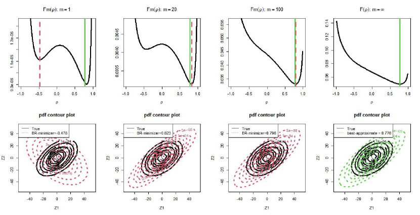
Figure 3: At the top, red line represents the selected minimizer of each $F_{m}$ by R function optimize, which may be a non-global local minimizer, whereas the green line represents the best $\bar{\mathcal{E}}$-approximation. The bottom plots represent the corresponding pdf contour plots.

C.3.3 An example that satisfies Assumption 4.2

We can arbitrarily choose the cardinality $|\mathcal{S\times A}|\in\mathbb{N}$ and discount rate $\gamma\in(0,1)$. We can also assume any behavior and target policies $b$ and $\pi$. Conditioned on $s,a$, its reward follows $R(s,a)\sim N(0,\tilde{\theta})$ with $\tilde{\theta}>0$, which leads the target distribution $\Upsilon_{\pi}(s,a)$ to follow $N(0,\tilde{\theta}/(1-\gamma^{2}))$ at all $s,a\in\mathcal{S\times A}$. We select a model $\Upsilon_{\theta}$ where $\Upsilon_{\theta}(s,a)$ being the probability measure of $N(0,\theta/(1-\gamma^{2}))$ with $\theta\in\Theta\subset[0,\infty)$ for all $s,a\in\mathcal{S\times A}$. Then we have

$$F(\theta) =\bar{\mathcal{E}}(\Upsilon_{\theta},\Upsilon_{\pi})=\sum_{s,a}b_{\mu}(s,a)\cdot\mathcal{E}\{\Upsilon_{\theta}(s,a),\Upsilon_{\pi}(s,a)\}=\frac{2}{\sqrt{\pi}}\cdot\frac{1}{\sqrt{1-\gamma^{2}}}\cdot(\sqrt{2(\theta+\tilde{\theta})}-\sqrt{\theta}-\sqrt{\tilde{\theta}}).$$

For simplicity, let us assume $\tilde{\theta}=1$ and $\Theta=[0,2]$. Since we have $F^{\prime}(1)=0$ and $F^{\prime\prime}(1)=\frac{1}{4}\cdot\sqrt{\frac{1}{\pi\cdot(1-\gamma^{2})}}>0$, this satisfies Assumption 4.2.

C.3.4 Rate Mismatch between Theorem 3.3 and B.5.3

Below Theorem 4.3, we have mentioned that the theoretical result for nonrealizable scenario B.5.3 does not degenerate to Theorem 3.3 under realizable setting with $m=1$. There are two factors that slow down the convergence rate throughout the proof of Appendix B.

First, we are forming multi-step trajectories by resampling from the collected data $\{(s_{i},a_{i},r_{i},s_{i}^{\prime})\}_{i=1}^{N}$, as mentioned before (20). This practice of re-using the samples no longer guarantees the independence of the data that we use. Then we cannot make use of common tricks for showing sample mean converging to the population mean (e.g. Theorems C.1, C.2, C.3 employed in A.6.3 and A.6.4), since since they require independence of samples. Therefore, we resort to another trick, that is Lemma B.3 that resembles triangular inequality, but slows down the rate by $1/2$.

Second, in non-realizable cases, the converging target is no longer the true distribution. Instead, we compromise our goal into the “best approximation” $\Upsilon_{\tilde{\theta}}$ defined in (19). That being said, Theorem 3.3, which only required us to derive the convergence rate of estimated Bellman residual (our objective function), is not enough now. Therefore, unlike realizable scenario, it requires one additional procedure, which is obtaining convergence of the minimizing parameter. This leads us to take into account the function $\psi(\cdot)$ in (145), which further slows down the rate by $1/q$.

Due to the aforementioned reasons, the rate in non-realizable scenario is slower than realizable scenario by $1/(2q)$, that is $\sqrt{\log N/N}$ verses $\sqrt[4q]{\log N/N}$.

C.3.5 Regarding linear MDP

Linear MDP may be useful in expanding our method into continuous state-action space by expressing the transition probability and reward distribution as linear combinations of multiple features $\phi(\cdot,\cdot):\mathcal{S\times A}\rightarrow\mathbb{R}^{n}$. To elaborate, it may allow us to construct an unbiased estimate of energy distance for continuous state-action space, where a single $s,a$ cannot be observed twice or more (almost surely). In such cases, our current estimation in Equation (9) leads to a biased estimate of the third term of expansion of $\mathcal{E}\{\Upsilon_{\theta}(s,a),\mathcal{T}^{\pi}\Upsilon_{\theta}(s,a)\}$ shown in Equation (8), which is $\mathbb{E}\|R_{\alpha}+\gamma\cdot Z_{\alpha}(S_{\alpha}^{\prime},A_{\alpha}^{\prime};\theta)-R_{\beta}-\gamma\cdot Z_{\beta}(S_{\beta}^{\prime},A_{\beta}^{\prime};\theta)\|$. Here, we have $(R_{\alpha},S_{\alpha}^{\prime}),(R_{\beta},S_{\beta}^{\prime})\sim p(\cdots|s,a)$ and $A_{\alpha}^{\prime}\sim\pi(\cdot|S_{\alpha}^{\prime})$, $A_{\beta}^{\prime}\sim\pi(\cdot|S_{\beta}^{\prime})$, where $\alpha,\beta$ are for indicating independent copies. According to our current way of estimation (9), our estimate becomes $\mathbb{E}\|\gamma\cdot Z_{\alpha}(s^{\prime},A_{1}^{\prime};\theta)-\gamma\cdot Z_{\beta}(s^{\prime},A_{2}^{\prime};\theta)\|$ with $A_{1}^{\prime},A_{2}^{\prime}\sim\pi(\cdot|s^{\prime})$ being independent. This is because the terms $\hat{R}_{\alpha}=r$ and $\hat{R}_{\beta}=r$ have the same value, and are thereby cancelled out when there is only a single observation $(s,a,r,s^{\prime})$. This bias might be prevented if we can estimate the distribution of terms $\hat{R}_{\alpha},\hat{R}_{\beta}\sim\hat{p}(\cdots|s,a)$ (for $s,a$ that was observed only once) by expressing them with features. In addition, leveraging the structure of the linear MDP may improve the efficiency of our method. It will be interesting to see what the structure of return distribution induced by the linear MDP is, which requires further investigation.

Appendix D Other Materials

D.1 Comparison between DRL methods in details

In Table 3, we specified the “contractive distance,” which is the distance that makes Bellman operator contractive, or that compined with projected operators $\Pi_{\mathcal{C}},\Pi_{\mathbb{W}_{1}}:\mathcal{P}(\mathbb{R}^{d})^{\mathcal{S\times A}}\rightarrow\mathcal{P}(\mathbb{R}^{d})^{\mathcal{S\times A}}$. Each of these is the projection towards categorized support items [1] and with respect to Wassserstein-1 metric [6], respectively. Then we compared them with the objective functions, and most methods had misalignment between these two. That is, the contraction and objective function are either based upon different distances, or their ways of extension (expecation or supremum) are different. FLE [26] and EBRM are the only two methods that could overcome this issue, which allowed them to prove convergence of the estimation towards some target with a certain rate (Table 4). In addition, EBRM can be applied when reward is multi-dimensional $d\geq 2$, unlike quantile/expectile-based methods (QRTD, IQN, FQF, EDRL).

Table 3: Comparison between Contractive Distances and Objective Functions

Method	Operator & Contractive Distance	Objective Function
Categorical	$\mathcal{T}^{\pi}$: Wasserstein-1	Cross Entropy
algorithm	(supremum-extended)	(expectation-extended)
[1, 16]	$\Pi_{\mathcal{C}}\mathcal{T}^{\pi}$: Cramer distance
	(supremum-extended)
QRTD [5]
IQN [5]	$\Pi_{\mathbb{W}_{1}}\mathcal{T}^{\pi}$: Wasserstein-$\infty$	quantile Huber Loss
FQF [27]	(supremum-extended)	(expectation-extended)
EDRL [17]	no additional result	Expectile Regression Loss
	about contraction	(expectation-extended)
MMDRL [15]	$\mathcal{T}^{\pi}$: supremum-extended $\text{MMD}_{k}$	$\text{MMD}_{k}^{2}$
	(unrectified kernel)	(expectation-extended)
	(supremum-extended)
SinkhornDRL [20]	$\mathcal{T}^{\pi}$: Sinkhorn Divergence	Sinkhorn Divergence
	(supremum-extended)	(expectation-extended)
MD3QN [28]	$\mathcal{T}^{\pi}$: Wasserstein-$p$ ($p\geq 1$)	$\text{MMD}_{k}^{2}$ (Gaussian kernel)
	(supremum-extended)	(expectation-extended)
FLE [26]	$\mathcal{T}^{\pi}$: Squared Wasserstein-$p$ ($p\geq 1$)	log-Likelihood
	(expectation-extended)	(expectation-extended)
	$\mathcal{T}^{\pi}$ , $(\mathcal{T}^{\pi})^{m}\ (m\geq 2)$
EBRM	: Energy Distance	Energy Distance
(our method)	(expectation-extended)	(expectation-extended)
	(not exactly contraction: Theorem 2.2)

Table 4: Convergence towards some target distribution

Method	Convergence towards Target
Categorical	$(\Pi_{\mathcal{C}}\mathcal{T}^{\pi})^{m}\Upsilon_{0}\rightarrow\Upsilon_{C}\neq\Upsilon_{\pi}$ as $m\rightarrow\infty$
algorithm	Convergence rate not suggested
[1, 16]	(Assumption: bounded reward)
QRTD [5]
IQN [5]	NA
FQF [27]
EDRL [17]	only implies convergence of expectation, not the distribution.
MMDRL [15]	NA
SinkhornDRL [20]	NA
MD3QN [28]	NA
FLE [26]	$(\mathcal{T}^{\pi})^{m}\Upsilon_{0}\rightarrow\Upsilon_{\pi}$ as $m\rightarrow\infty$
	Convergence rate suggested
	(Assumption: bounded reward, completeness)
EBRM	Convergence towards truth / best approximation
(our method)	Convergence rate suggested

D.2 Realizable and Nonrealizable Models

D.2.1 Introduction of Simulation Settings

With the state-action space in Section 5, let us assume that $s,a$ is given. The agent moves by one in the direction of $a\in\{-1,1\}$, that is $s^{\prime}=s+a$ (value of which fully determines the reward distribution (166)). If the agent is already blocked by the direction, that is $(s,a)=(1,-1)$ or $(s,a)=(30,1)$, it stays at the same position $s^{\prime}=s$. With given values of $A_{0}>0,p_{0}\in(0,1),\sigma_{0}^{2}>0$, our transition $p(r,s^{\prime}|s,a)$ is characterized by:

$$\text{Conditioned on }S+A=k,\ R\sim N(\mu_{k},\sigma_{0}^{2})\quad\text{where}\quad\mu_{k}=\begin{cases}A_{0}\cdot p_{0}^{k}&(k=0,\cdots,30)\\ 0&(k=31)\end{cases}$$ (166)

and $$S^{\prime}=k\ \text{if }k\in\{1,\cdots,30\},\quad S^{\prime}=30\ \text{if }k=31,\quad S^{\prime}=1\ \text{if }k=0.$$

We assume infinite-horizontal setting. Following the environment (166) and target policy (22), we have $\Upsilon_{\pi}(s,a)$ to be normal distributions, with expectation and variance as follows,

$$\mathbb{E}\big{\{}Z_{\pi}(i,-1)\big{\}}=A_{0}\cdot p_{0}^{i-1}\cdot\frac{1-(\gamma p_{0})^{32-i}}{1-\gamma p_{0}}\ \ (i\geq 2),\quad\mathbb{V}\big{\{}Z_{\pi}(i,\pm 1)\big{\}}=\frac{\sigma_{0}^{2}}{1-\gamma^{2}}\ \ (i\geq 1),$$ (167)

$$\mathbb{E}\big{\{}Z_{\pi}(i,1)\big{\}}=A_{0}\cdot p_{0}^{i+1}\cdot\frac{1-(\gamma p_{0})^{30-i}}{1-\gamma p_{0}}\ \ (i\geq 1),\quad\mathbb{E}\big{\{}Z_{\pi}(1,-1)\big{\}}=A_{0}+\gamma\cdot\mathbb{E}\big{\{}Z_{\pi}(1,1)\big{\}}.$$

We always let $A_{0}=100$, $p_{0}=0.9$ throughout the simulations.

First, we assumed a realizable scenario where the correct model (167) is known (Appendix D.2.2), only not knowing the values of $A_{0}$, $p_{0}$. Here, we always assumed $\gamma=0.99$ and tried two settings with $\sigma_{0}^{2}=20$ and $\sigma_{0}^{2}=5000$. Second, we always tried the non-realizable scenario where there is a model misspecification (168), as will be demonstrated in Appendix D.2.3. Here, we always assumed $\sigma^{2}=20$, trying $\gamma=0.50$ and $\gamma=0.99$.

D.2.2 Realizable Scenario

In the realizable scenario, we assume that Equations (167) are known, except the values of $A_{0}=100$ and $p_{0}=0.9$. The distributions can be plotted as Figure 4, each for $\sigma_{0}^{2}=20$ and $\sigma_{0}^{2}=5000$.

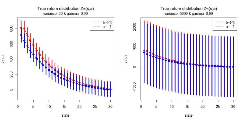
Figure 4: Red and blue represent the distributions of $Z_{\pi}(s,-1)$ and $Z_{\pi}(s,1)$ respectively. The dots indicate the expectation values and the vertical bars include (Mean$\pm$ 3$\cdot$SD).

D.2.3 Non-realizable Scenario

On the other hand, in the non-realizable scenario, we assume that we are not aware of the true model (167). Instead, we assume that we are only aware of the decreasing trend demonstrated in Figure 4. That being said, we apply the following linear model that holds for all $1\leq i\leq 30$. with four different parameters $\beta_{L},\beta_{R},\beta_{1}\in\mathbb{R}$, $\sigma^{2}>0$,

$$\mathbb{E}\big{(}Z_{\pi}(i,-1)\big{)}=\beta_{L}+\beta_{1}\cdot i,\ \ \mathbb{E}\big{(}Z_{\pi}(i,1)\big{)}=\beta_{R}+\beta_{1}\cdot i,\ \ \mathbb{V}\big{(}Z_{\pi}(i,\pm 1)\big{)}=\frac{\sigma^{2}}{1-\gamma^{2}}.$$ (168)

This means that the distributions (conditioned on each $s,a$) have common variance, common slope in expectations, but different $y$-intercepts in expectations.

We always assumed $\sigma_{0}^{2}=20$ and tried two different settings, $\gamma=0.50$ and $\gamma=0.99$. Denoting the parameter as $\theta=(\beta_{L},\beta_{R},\beta_{1},\sigma^{2})$ and candidate space as $\Theta=\mathbb{R}\times\mathbb{R}\times\mathbb{R}^{-}\times\mathbb{R}^{+}$, the best approximation value $\tilde{\theta}$ that minimize the inaccuracy $\bar{\mathcal{E}}(\Upsilon_{\theta},\Upsilon_{\pi})$ are calculated in Table 5. They are visualized in Figure 5 (true distributions $\Upsilon_{\pi}$ on left and best approximations $\Upsilon_{\tilde{\theta}}$ on right).

Table 5: Best approximation values and minimum inaccuracy

Scenario	$\beta_{L}$	$\beta_{R}$	$\beta_{0}$	$\sigma^{2}$	Minimum $\bar{\mathcal{E}}$-inaccuracy
$\gamma=0.50$	126.216	116.614	-4.571	203.099	13.238
$\gamma=0.99$	610.970	562.782	-23.246	149.866	63.216

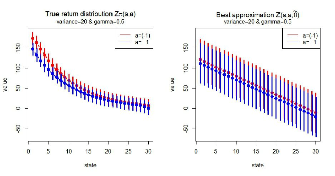
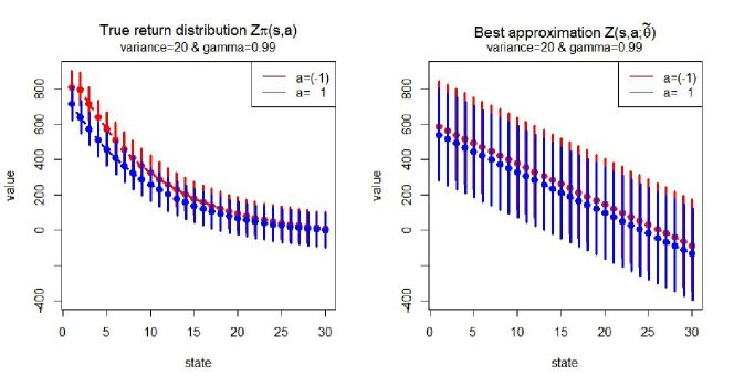
Figure 5: Red and blue represent the distributions of $Z_{\pi}(s,-1)$ and $Z_{\pi}(s,1)$, or $Z(s,-1;\tilde{\theta})$ and $Z(s,1;\tilde{\theta})$, respectively. The dots indicate the expectation values and the vertical bars include (Mean$\pm$ 3$\cdot$SD).

D.3 Tuning parameters of each method

D.3.1 EBRM

Energy distance (7) is calculated via numerical integration given the densities of the probability measures. Here is the algorithm of choosing the step level $m$, solely based on the observed data. The basic skeleton is based on SLOPE suggested by Su [19] based on Lepski’s rule [10]. Starting from large enough $m$, we can decrease it until the intersection of the confidence intervals (formed with multiple bootstraps) becomes a null set.

Algorithm 3 Lepski’s rule of selecting step level $m$

$1=m_{0}<m_{1}<\cdots m_{K}$

Input: $\mathcal{D}=\{(s_{i},a_{i},r_{i},s_{i}^{\prime})\}_{i=1}^{N}$, $J$, $M$, $(m_{1},m_{2},\cdots,m_{K})$

Output: $m_{k}$

Estimate $\hat{\theta}$ with single-step estimation (12).

$k\leftarrow K+1$, $O_{K+1}\leftarrow[-\infty,\infty]$.

while $O_{k}\neq\varnothing$ do

     $k\leftarrow k-1$.

     if $k\neq 0$ then

         for $j=1,\cdots,J$ do

              Estimate $\hat{\theta}_{m_{k},j}^{(B)}$ with multi-step estimation (21) of step level $m=m_{k}$.

              Calculate $\hat{e}_{k,j}:=\hat{\bar{\mathcal{E}}}(\Upsilon_{\hat{\theta}},\Upsilon_{\hat{\theta}_{m_{k},j}^{(B)}})$.

         end for

         Calculate the sample mean ($\hat{\mu}_{k}$) and variance ($\hat{s}_{k}$) of $\hat{e}_{k,j}$ ($j=1,\cdots,J$).

         Calculate $I_{k}:=[\hat{\mu}_{k}\pm 1.96\cdot\hat{s}_{k}]$.

         $O_{k}\leftarrow O_{k+1}\cap I_{k}$.

     else

         $O_{k}\leftarrow\varnothing$.

     end if

end while

Throughout multiple simulations in each setting (D.2.2 and D.2.3) for each sample size $N$ (demonstrated in D.4), it is rigorous to pick its own optimal step level $m$. However, since they do not differ significantly, we picked the step level $m$ via Algorithm 3 based on the first simulated data, and used the same value of $m$ throughout the remaining simulations, in order to save computational burden. We applied the algorithm with $M=N$ and $J=50$. Obviously, we had to try larger values of $(m_{1},\cdots,m_{K})$ for non-realizable scenario with $\gamma=0.99$ than $\gamma=0.50$. However, to avoid numerical issues in integration caused by extremely small $\gamma^{m}$, we limited the choice of step levels into $m\leq 4$ ($\gamma=0.50$) and $m\leq 250$ ($\gamma=0.99$). The corresponding intervals $I_{k}$ are visualized in Figures 7 and 6, and the selected step level $m_{*}$ is specified in Table 6.

Table 6: Selected step level $m_{*}$

Realizable	$N=500$	$N=1000$	$N=2000$	$N=5000$	$N=10000$	$N=20000$
$\sigma^{2}=20$	1	1	1	1	1	1

Realizable	$N=2000$	$N=5000$	$N=10000$	$N=20000$	$N=50000$	$N=10^{5}$
$\sigma^{2}=5000$	1	1	1	1	1	1

Non-realizable	$N=2000$	$N=3000$	$N=5000$	$N=10000$
$\gamma=0.50$	1	1	1	2
$\gamma=0.99$	100	160	200	250

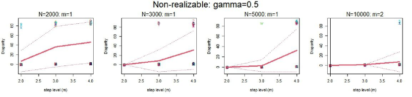
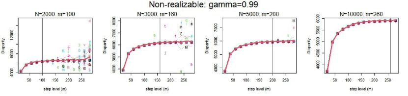
Figure 6: Non-realizable, $\gamma=0.50$ (top 4 figures) and $\gamma=0.99$ (bottom 4 figures). To prevent numerical issues, we set an upper limit $m\leq 250$ in $\gamma=0.99$, so we have $m_{*}=250$ for $N=10000$.

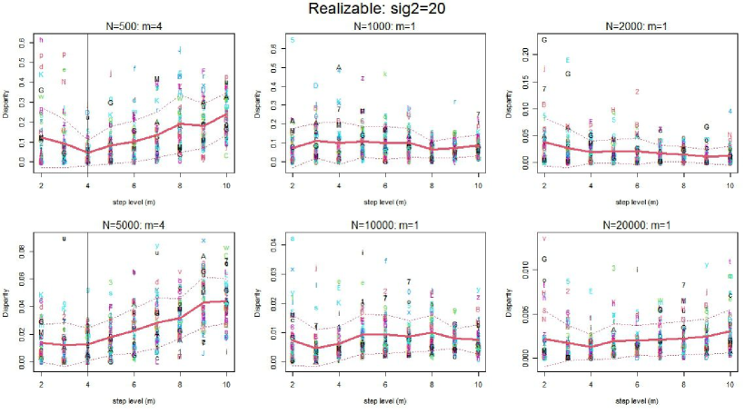
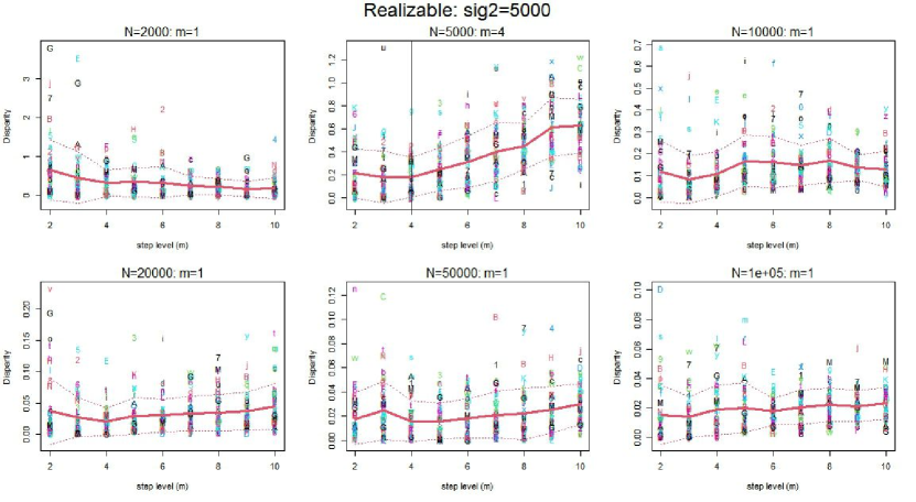
Figure 7: Realizable, $\sigma_{0}^{2}=20$ (top 6 figures) $\sigma_{0}^{2}=5000$ (bottom 6 figures)

D.3.2 FLE

They did not officially suggest a rule of selecting the number of partitions $T$ and their sizes $|\mathcal{D}_{1}|,\cdots,|\mathcal{D}_{T}|$ in FLE, so we utilized its asymptotic result (Corollary 4.14 by [26]) to construct the following heuristic rule based on pre-determined values of $N_{0}$, $T_{0}$, and $l>0$,

$$T(N)\buildrel let\over{=}\log_{\big{(}{\frac{1}{\gamma}}\big{)}^{1-\frac{1}{2l}}}\bigg{\{}\frac{1}{C}\cdot\bigg{(}\frac{N}{\log N}\bigg{)}^{\frac{1}{2l}}\bigg{\}},\quad\mbox{where }C_{0}>0\text{ satisfies }T(N_{0})=T_{0}.$$ (169)

Note that larger value of $l$ slows down the increasing speed of $T(N)$. In addition, we prevent the number of partition $T$ from becoming too small, we put a lower bound $\tilde{T}$

$$T^{*}(N)=\max\bigg{\{}\tilde{T},\lfloor T(N)\rfloor\bigg{\}}.$$

Then each partition has $|\mathcal{D}_{t}|=\lfloor N/T^{*}(N)\rfloor$, but may have some remaining observations when $N$ is not divisble by the chosen $T$. In this case, we included all the remaining observations into the last partition $\mathcal{D}_{T}$. The tuning parameters are chosen after multiple numerical experiments, and the following choice (Table 7) seemed to work best.

Table 7: Tuning parameters of FLE

Sample size	$l$	$N_{0}$	$T_{0}$	$\tilde{T}$
realizable, $\sigma^{2}=50$	10	2000	25	15
realizable, $\sigma^{2}=5000$	10	20000	25	15
non-realizable, $\gamma=0.50$	0.7	3000	10	10
non-realizable, $\gamma=0.99$	10	2000	25	15

D.3.3 QRTD

QRTD [6] was originally designed for updating value distributions only conditioned on the state $s\in\mathcal{S}$, not the action $a\in\mathcal{A}$ (refer to their Equation (12)). However, we could readily develop it towards the action-value distributions conditioned on $s,a\in\mathcal{S\times A}$. That is, with $\tau_{i}\in[0,1]$ ($1\leq i\leq N_{\tau}$) being cdf values and $\theta_{i}(s,a)$ being the corresponding quantile value, they model the distribution to be uniform across $\theta_{i}(s,a)$,

$$Z_{\theta}(s,a)=\frac{1}{N_{\tau}}\sum_{i=1}^{N_{\tau}}\delta_{\theta_{i}(s,a)}.$$

Analogously to their original version, we update it as follows, whenever a single new observation $(s,a,r,s^{\prime})$ is collected,

$$\text{Sample }i\sim\text{Unif}\big{\{}1,\cdots,N_{\tau}\big{\}}$$ (170)

$$\theta_{i}(s,a)\leftarrow\theta_{i}(s,a)+\alpha_{0}\cdot\{{\tau}_{i}-\mathbf{1}(r+\gamma z^{\prime}<\theta_{i}(s,a))\}\quad\text{where }z^{\prime}\sim Z_{\theta}(s^{\prime},a^{\prime}),\ a^{\prime}\sim\pi(\cdot|s^{\prime}).$$

The number of quantiles is chosen to be 99, that is $\tau_{i}=i/100$ $(1\leq i\leq 99)$. As Dabney mentioned [6], we repeat the procedure (170) for multiple times within each iteration, which we let to be the same as $N_{\tau}=99$ times in our case. We chose $\alpha_{0}=5$ for $\sigma^{2}=20$ and $\alpha_{0}=2$ for $\sigma^{2}=5000$ of realizable cases, since they worked fine empirically.

D.4 Simulation Results

D.4.1 Realizable Scenario

As was mentioned in Section 5, we included three different inaccuracy measures (Tables 8–10). Expectation-extended energy distance $\bar{\mathcal{E}}$ is the one that we have used in our main theoretical results (Theorems 3.3 and 4.3). For the sake of fairness, we also included expectation-extended (5) Wasserstein-1 metric $\overline{\mathbb{W}}_{1}$, based on that Wasserstein-1 metric plays an important role in DRL literature (Table 3). Lastly, we also used $\mathbb{W}_{1}$ to compare the marginal distributions $\Upsilon^{marginal}$ which is defined as the mixture of $\{\Upsilon(s,a):s,a\in\mathcal{S\times A}\}$ with weights $\{b_{\mu}(s,a):s,a\in\mathcal{S\times A}\}$, which was used in Corollary 4.14 by Wu [26]. Measurement of the second and third inaccuracies using $\overline{\mathbb{W}}_{1}$ and $\mathbb{W}_{1}$ was approximated via R package transport using randomly generated samples.

With all three inaccuracy measures, we could see that EBRM gave us most accurate results. Here are brief reasons that explain the difference. QRTD resorts to a finite number of quantiles to represent the estimated distribution, which is limited in expressing continuous densities. FLE is not not utilizing the closed-form probability measure in each update. Whenever they update their estimation at $t$-th iteration, they sample finitely many samples from the previous estimate $\Upsilon_{\theta_{t-1}}(s,a)$, which follows with approximation error. Since EBRM uses the closed-form densities in expressing continuous random variables, it could outperform QRTD and FLE.

Table 8: Mean $\bar{\mathcal{E}}$-inaccuracy (standard deviation in parenthesis) over 100 simulations under realizability ($\gamma=0.99$) for $\sigma_{0}^{2}=20$ (top) versus $\sigma_{0}^{2}=5000$ (bottom). Smallest inaccuracy values are in boldface.

Sample size	$500$	$1000$	$2000$	$5000$	$10000$	$20000$
EBRM	0.164	0.066	0.046	0.019	0.008	0.005
	(0.227)	(0.087)	(0.060)	(0.022)	(0.010)	(0.007)
FLE	17.729	8.802	5.533	2.385	1.220	0.761
	(15.438)	(9.175)	(6.448)	(2.883)	(1.618)	(0.888)
QRTD	149.338	64.259	48.679	46.032	49.402	49.965
	(25.221)	(23.160)	(34.323)	(30.909)	(34.617)	(31.458)

Sample size	$2000$	$5000$	$10000$	$20000$	$50000$	$100000$
EBRM	0.728	0.301	0.128	0.074	0.028	0.018
	(0.920)	(0.354)	(0.167)	(0.105)	(0.034)	(0.022)
FLE	24.603	14.482	6.528	5.062	2.662	1.522
	(25.768)	(16.101)	(7.814)	(6.007)	(3.386)	(1.985)
QRTD	105.274	75.173	70.483	74.398	73.533	77.358
	(11.728)	(21.515)	(33.965)	(52.039)	(70.004)	(62.997)

Table 9: Mean $\overline{\mathbb{W}}_{1}$-inaccuracy (standard deviation in parenthesis) over 100 simulations under realizability ($\gamma=0.99$) for $\sigma_{0}^{2}=20$ (top) versus $\sigma_{0}^{2}=5000$ (bottom). Smallest inaccuracy values are in boldface.

Sample size	$500$	$1000$	$2000$	$5000$	$10000$	$20000$
EBRM	2.176	1.523	1.339	0.985	0.782	0.706
	(1.442)	(0.864)	(0.651)	(0.388)	(0.227)	(0.171)
FLE	22.912	15.755	12.374	8.036	5.694	4.590
	(12.774)	(9.229)	(7.843)	(5.091)	(3.773)	(2.856)
QRTD	105.561	64.290	56.739	54.397	57.145	57.953
	(12.418)	(13.936)	(23.716)	(22.259)	(24.314)	(22.252)

Sample size	$2000$	$5000$	$10000$	$20000$	$50000$	$100000$
EBRM	21.221	15.532	12.371	11.178	9.971	9.694
	(10.337)	(6.117)	(3.595)	(2.717)	(1.143)	(0.802)
FLE	101.232	79.628	53.745	49.426	35.453	27.493
	(58.586)	(46.772)	(33.948)	(29.198)	(21.370)	(16.038)
QRTD	274.405	236.383	223.537	223.399	218.028	224.539
	(11.003)	(22.376)	(38.935)	(63.145)	(82.134)	(76.002)

Table 10: Mean $\mathbb{W}_{1}$-inaccuracy of marginal distributions (standard deviation in parenthesis) over 100 simulations under realizability ($\gamma=0.99$) for $\sigma_{0}^{2}=20$ (top) versus $\sigma_{0}^{2}=5000$ (bottom). Smallest inaccuracy values are in boldface.

Sample size	$500$	$1000$	$2000$	$5000$	$10000$	$20000$
EBRM	2.052	1.406	2.052	0.843	0.629	0.508
	(1.524)	(1.005)	(0.778)	(0.556)	(0.350)	(0.255)
FLE	22.835	15.694	12.328	8.013	5.596	4.591
	(12.810)	(9.272)	(7.859)	(5.113)	(3.786)	(2.945)
QRTD	97.856	56.694	47.738	45.764	49.851	49.877
	(13.235)	(14.905)	(25.251)	(25.656)	(27.463)	(25.945)

Sample size	$2000$	$5000$	$10000$	$20000$	$50000$	$100000$
EBRM	18.021	11.613	7.528	5.441	3.607	3.062
	(12.227)	(8.077)	(5.306)	(4.184)	(2.487)	(1.981)
FLE	94.556	71.430	46.740	44.915	31.774	23.378
	(62.630)	(51.205)	(36.986)	(31.905)	(23.190)	(18.076)
QRTD	247.308	198.257	191.908	195.787	194.908	202.076
	(16.843)	(29.911)	(48.057)	(73.533)	(91.526)	(86.031)

D.4.2 Non-realizable Scenario

Now we tried non-realizable settings with the misspecified model (168) of Section D.2.3, based on tuning parameters determined in Tables 6 and 7. Since the point of this experiment is to see how each method can perform with a misspecified model. we excluded QRTD, which does not have any model assumption on the return distributions. We could see in Table 11 that EBRM approached the minimum possible level of Energy Distance (13.327 for $\gamma=0.50$ and 63.216 for $\gamma=0.99$) as we increased the sample size $N$. This forms contrast with FLE that even deteriorated as sample size grows, which we can supposedly attribute to huge violation of completeness that FLE is based upon.

Supposedly, the malfunctioning of FLE in Tables 11–13 (under $\gamma=0.99$) can be attributed to its completeness assumption (Assumption 4.12 of FLE [26]). Since completeness is a stronger statement than realizability, this implies that violation of realizability leads to more severe violation of completeness. This becomes even more severe when we are given a large discount rate $\gamma=0.99$, since it makes the extent of non-realizability even larger. Through this, we can indirectly ascertain the importance of relaxing completeness assumption, which is widely assumed in the literature of reinforcement learning, and EBRM succeeded in this.

Table 11: Mean $\bar{\mathcal{E}}$-inaccuracy (standard deviation in parenthesis) under non-realizability for $\gamma=0.50$ (top) VS $\gamma=0.99$ (bottom). Smallest inaccuracy values are in boldface. Minimum possible $\bar{\mathcal{E}}$-inaccuracy values are 13.237 ($\gamma=0.50$) and 63.216 ($\gamma=0.99$).

Sample size	$2000$	$3000$	$5000$	$10000$
EBRM	14.323	14.306	14.299	13.544
	(0.209)	(0.152)	(0.128)	(0.065)
FLE	15.199	15.206	15.171	15.171
	(0.490)	(0.374)	(0.306)	(0.227)

Sample size	$2000$	$3000$	$5000$	$10000$
EBRM	124.162	96.462	82.102	70.381
	(42.117)	(48.178)	(37.470)	(9.503)
FLE	448.837	488.535	625.682	781.287
	(38.256)	(43.141)	(41.130)	(41.192)

Table 12: Mean $\overline{\mathbb{W}}_{1}$-inaccuracy (standard deviation in parenthesis) under non-realizability for $\gamma=0.50$ (top) VS $\gamma=0.99$ (bottom). Smallest inaccuracy values are in boldface.

Sample size	$2000$	$3000$	$5000$	$10000$
EBRM	19.245	19.232	19.202	17.589
	(0.405)	(0.308)	(0.258)	(0.240)
FLE	15.036	15.049	15.047	15.037
	(0.392)	(0.330)	(0.256)	(0.197)

Sample size	$2000$	$3000$	$5000$	$10000$
EBRM	168.231	108.196	91.621	82.293
	(24.009)	(24.756)	(17.601)	(5.490)
FLE	258.802	280.319	350.925	433.074
	(19.127)	(21.680)	(20.697)	(21.534)

Table 13: Mean $\mathbb{W}_{1}$-inaccuracy of marginal distributions (standard deviation in parenthesis) under non-realizability for $\gamma=0.50$ (top) VS $\gamma=0.99$ (bottom). Smallest inaccuracy values are in boldface.

Sample size	$2000$	$3000$	$5000$	$10000$
EBRM	14.098	14.088	14.087	13.218
	(0.227)	(0.167)	(0.142)	(0.093)
FLE	13.954	13.977	13.968	13.970
	(0.359)	(0.292)	(0.234)	(0.184)

Sample size	$2000$	$3000$	$5000$	$10000$
EBRM	106.850	84.839	73.338	66.560
	(39.076)	(29.761)	(17.974)	(5.392)
FLE	258.141	279.687	349.984	432.014
	(19.073)	(21.771)	(20.467)	(21.903)

References

- Bellemare et al. [2017] Bellemare, M. G., W. Dabney, and R. Munos (2017). A distributional perspective on reinforcement learning. In International conference on machine learning, pp. 449–458. PMLR.
- Bellemare et al. [2017] Bellemare, M. G., I. Danihelka, W. Dabney, S. Mohamed, B. Lakshminarayanan, S. Hoyer, and R. Munos (2017). The cramer distance as a solution to biased wasserstein gradients. arXiv preprint arXiv:1705.10743.
- Bradtke and Barto [1996] Bradtke, S. J. and A. G. Barto (1996). Linear least-squares algorithms for temporal difference learning. Machine learning 22, 33–57.
- Chen et al. [2021] Chen, Z., S. T. Maguluri, S. Shakkottai, and K. Shanmugam (2021). Finite-sample analysis of off-policy td-learning via generalized bellman operators. Advances in Neural Information Processing Systems 34, 21440–21452.
- Dabney et al. [2018] Dabney, W., G. Ostrovski, D. Silver, and R. Munos (2018). Implicit quantile networks for distributional reinforcement learning. In International conference on machine learning, pp. 1096–1105. PMLR.
- Dabney et al. [2018] Dabney, W., M. Rowland, M. Bellemare, and R. Munos (2018). Distributional reinforcement learning with quantile regression. In Proceedings of the AAAI Conference on Artificial Intelligence, Volume 32.
- Gretton et al. [2012] Gretton, A., K. M. Borgwardt, M. J. Rasch, B. Schölkopf, and A. Smola (2012). A kernel two-sample test. The Journal of Machine Learning Research 13(1), 723–773.
- Kohler and Lucchi [2017] Kohler, J. M. and A. Lucchi (2017). Sub-sampled cubic regularization for non-convex optimization. In International Conference on Machine Learning, pp. 1895–1904. PMLR.
- Lazic et al. [2020] Lazic, N., D. Yin, M. Farajtabar, N. Levine, D. Gorur, C. Harris, and D. Schuurmans (2020). A maximum-entropy approach to off-policy evaluation in average-reward mdps. Advances in Neural Information Processing Systems 33, 12461–12471.
- Lepskii [1991] Lepskii, O. (1991). On a problem of adaptive estimation in gaussian white noise. Theory of Probability & Its Applications 35(3), 454–466.
- Mnih et al. [2015] Mnih, V., K. Kavukcuoglu, D. Silver, A. A. Rusu, J. Veness, M. G. Bellemare, A. Graves, M. Riedmiller, A. K. Fidjeland, G. Ostrovski, et al. (2015). Human-level control through deep reinforcement learning. nature 518(7540), 529–533.
- Morimura et al. [2010] Morimura, T., M. Sugiyama, H. Kashima, H. Hachiya, and T. Tanaka (2010). Nonparametric return distribution approximation for reinforcement learning. In Proceedings of the 27th International Conference on Machine Learning (ICML-10), pp. 799–806.
- Morimura et al. [2012] Morimura, T., M. Sugiyama, H. Kashima, H. Hachiya, and T. Tanaka (2012). Parametric return density estimation for reinforcement learning. arXiv preprint arXiv:1203.3497.
- Nguyen et al. [2020] Nguyen, T. T., S. Gupta, and S. Venkatesh (2020). Distributional reinforcement learning with maximum mean discrepancy. Association for the Advancement of Artificial Intelligence (AAAI).
- Nguyen-Tang et al. [2021] Nguyen-Tang, T., S. Gupta, and S. Venkatesh (2021). Distributional reinforcement learning via moment matching. In Proceedings of the AAAI Conference on Artificial Intelligence, Volume 35, pp. 9144–9152.
- Rowland et al. [2018] Rowland, M., M. Bellemare, W. Dabney, R. Munos, and Y. W. Teh (2018). An analysis of categorical distributional reinforcement learning. In International Conference on Artificial Intelligence and Statistics, pp. 29–37. PMLR.
- Rowland et al. [2019] Rowland, M., R. Dadashi, S. Kumar, R. Munos, M. G. Bellemare, and W. Dabney (2019). Statistics and samples in distributional reinforcement learning. In International Conference on Machine Learning, pp. 5528–5536. PMLR.
- Sen [2018] Sen, B. (2018). A gentle introduction to empirical process theory and applications. Lecture Notes, Columbia University 11, 28–29.
- Su et al. [2020] Su, Y., P. Srinath, and A. Krishnamurthy (2020). Adaptive estimator selection for off-policy evaluation. In International Conference on Machine Learning, pp. 9196–9205. PMLR.
- Sun et al. [2022] Sun, K., Y. Zhao, Y. Liu, W. Liu, B. Jiang, and L. Kong (2022). Distributional reinforcement learning via sinkhorn iterations. arXiv preprint arXiv:2202.00769.
- Székely and Rizzo [2013] Székely, G. J. and M. L. Rizzo (2013). Energy statistics: A class of statistics based on distances. Journal of statistical planning and inference 143(8), 1249–1272.
- Van der Vaart [2000] Van der Vaart, A. W. (2000). Asymptotic statistics, Volume 3. Cambridge university press.
- Vershynin [2018] Vershynin, R. (2018). High-dimensional probability: An introduction with applications in data science, Volume 47. Cambridge university press.
- Wang et al. [2023] Wang, J., Z. Qi, and R. K. Wong (2023). Projected state-action balancing weights for offline reinforcement learning. The Annals of Statistics 51(4), 1639–1665.
- Wang et al. [2022] Wang, J., R. K. Wong, and X. Zhang (2022). Low-rank covariance function estimation for multidimensional functional data. Journal of the American Statistical Association 117(538), 809–822.
- Wu et al. [2023] Wu, R., M. Uehara, and W. Sun (2023). Distributional offline policy evaluation with predictive error guarantees. arXiv preprint arXiv:2302.09456.
- Yang et al. [2019] Yang, D., L. Zhao, Z. Lin, T. Qin, J. Bian, and T.-Y. Liu (2019). Fully parameterized quantile function for distributional reinforcement learning. Advances in neural information processing systems 32.
- Zhang et al. [2021] Zhang, P., X. Chen, L. Zhao, W. Xiong, T. Qin, and T.-Y. Liu (2021). Distributional reinforcement learning for multi-dimensional reward functions. Advances in Neural Information Processing Systems 34, 1519–1529.