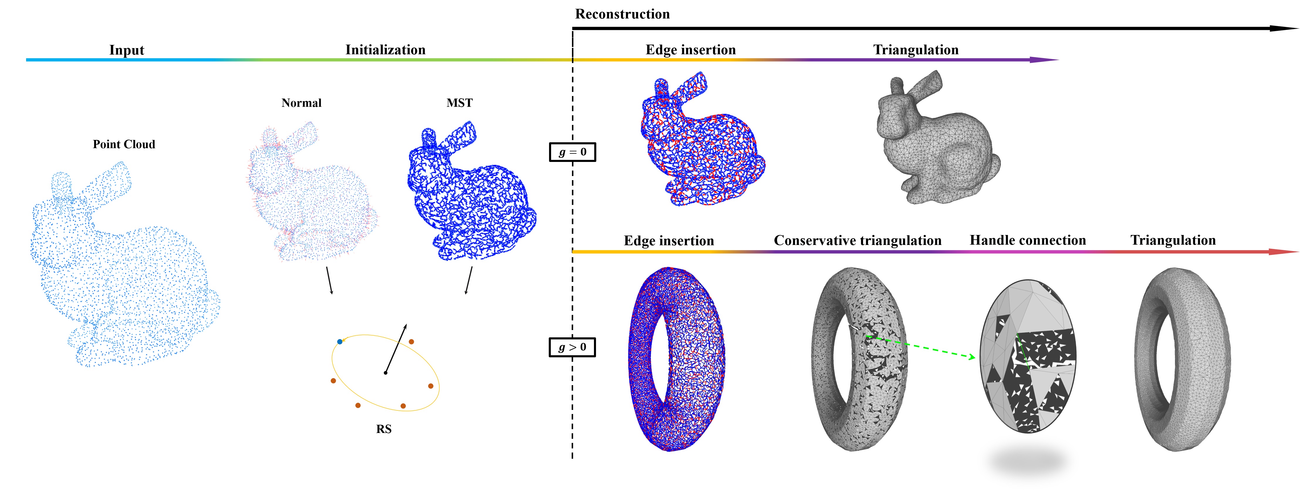
Figure 1. Pipeline Overview. The methodology comprises two key stages: initialization and reconstruction. During initialization, firstly, point normals are estimated and the minimum spanning tree (MST) is derived from the input point cloud. Based on those, the rotation system (RS) is constructed, where the blue point denotes the RS’s initial point. At the reconstruction stage, different pipelines follow up considering the possible genus number $g$ of the shape. The common operations are edge insertion and triangulation. For edge insertion, (red) edges are established based on the MST. The pipeline concludes with the reconstruction of a triangle mesh through triangulation. A possible high-genus shape needs two other operations to add handles to increase the genus.

Surface Reconstruction Using Rotation Systems

Abstract.

Inspired by the seminal result that a graph and an associated rotation system uniquely determine the topology of a closed manifold, we propose a combinatorial method for reconstruction of surfaces from points. Our method constructs a spanning tree and a rotation system. Since the tree is trivially a planar graph, its rotation system determines a genus zero surface with a single face which we proceed to incrementally refine by inserting edges to split faces and thus merging them. In order to raise the genus, special handles are added by inserting edges between different faces and thus merging them. We apply our method to a wide range of input point clouds in order to investigate its effectiveness, and we compare our method to several other surface reconstruction methods. We find that our method offers better control over outlier classification, i.e. which points to include in the reconstructed surface, and also more control over the topology of the reconstructed surface.

1. Introduction

Reconstruction of surfaces from 3D point clouds is a fundamental problem in geometry processing which continues to attract attention from researchers in the field. Undoubtedly, the main reason for this attention is the great practical utility of reconstruction algorithms due to the abundance of optical devices that can capture 3D point clouds, but it is also important to note that there are many variations of the problem, and the problem is ill-posed. All of these factors contribute to a large number of reconstruction methods with different strengths and weaknesses.

The ill-posed nature of the problem is due to the fact that there is generally no unique solution. Even if we restrict ourselves to only consider methods which connect all points to form a 2-manifold orientable triangle mesh, the number of possible solutions is immense for realistic input sizes. While it is trivial to connect a point to its $k$ nearest neighbors to form a graph, it is far from trivial to form a triangle mesh from this collection of edges, precisely due to the aforementioned combinatorial complexity. However, if we require the output triangle mesh to have disk topology, graph theory provides a solution, that to the best of our knowledge has not been considered before. The restriction to disk topology would be problematic, but we show how it is possible to relax this restriction in order to obtain meshes with boundary curves and of arbitrary genus.

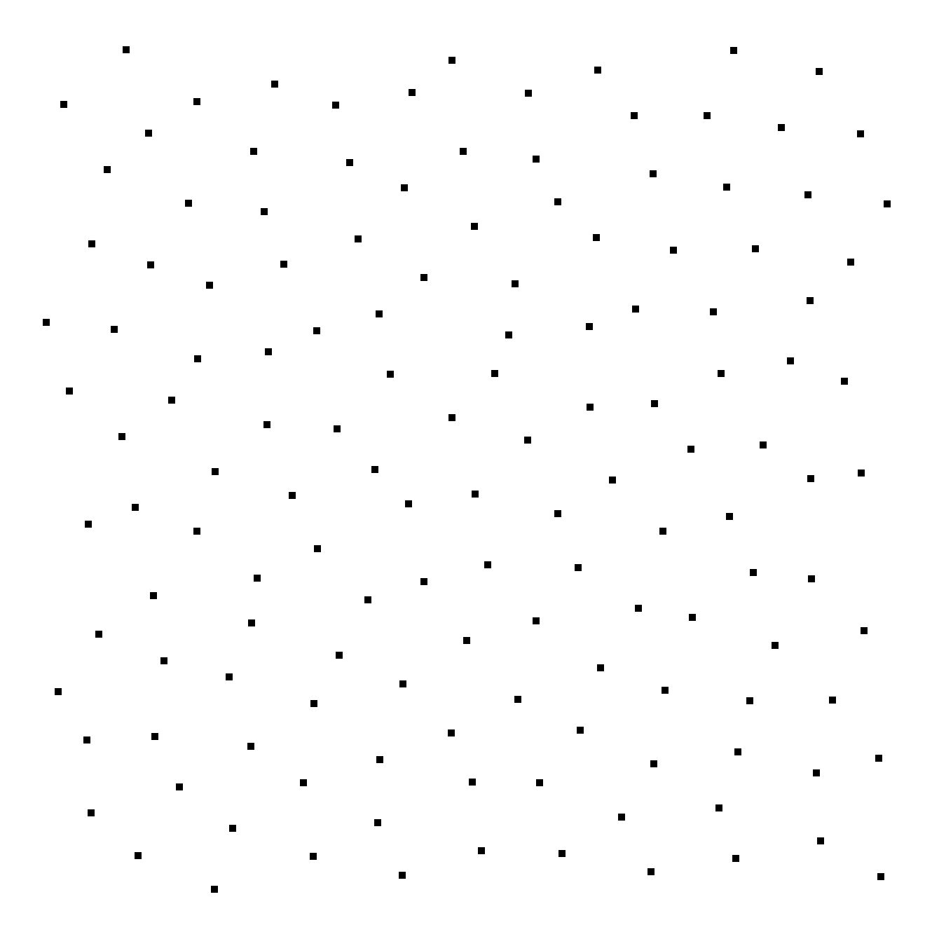
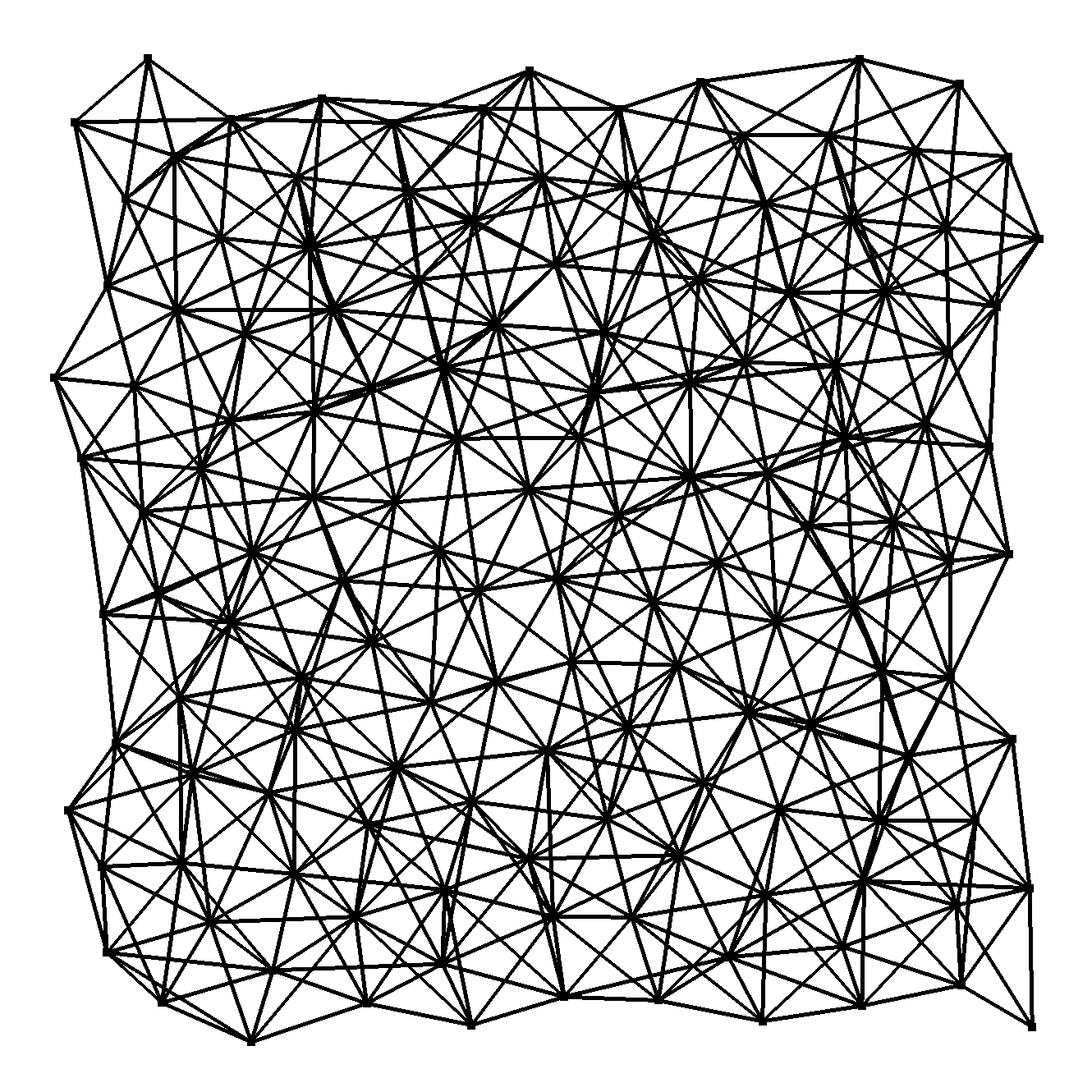
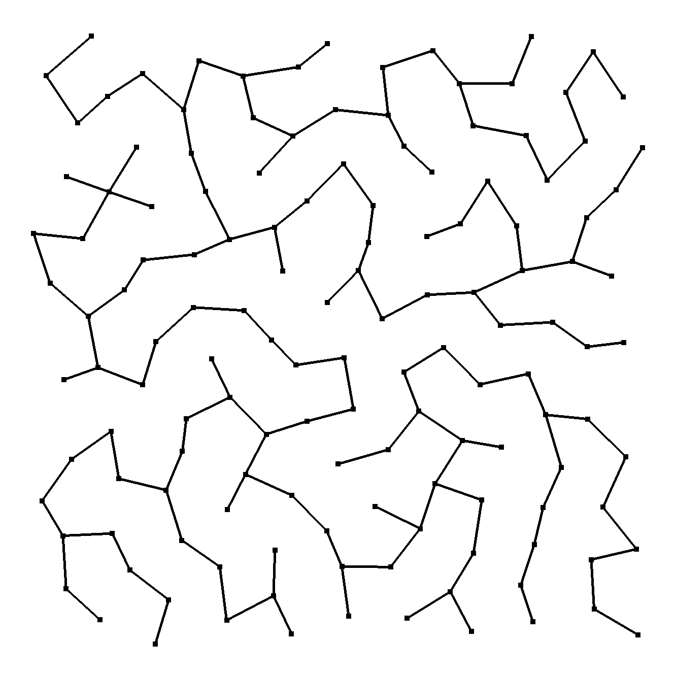
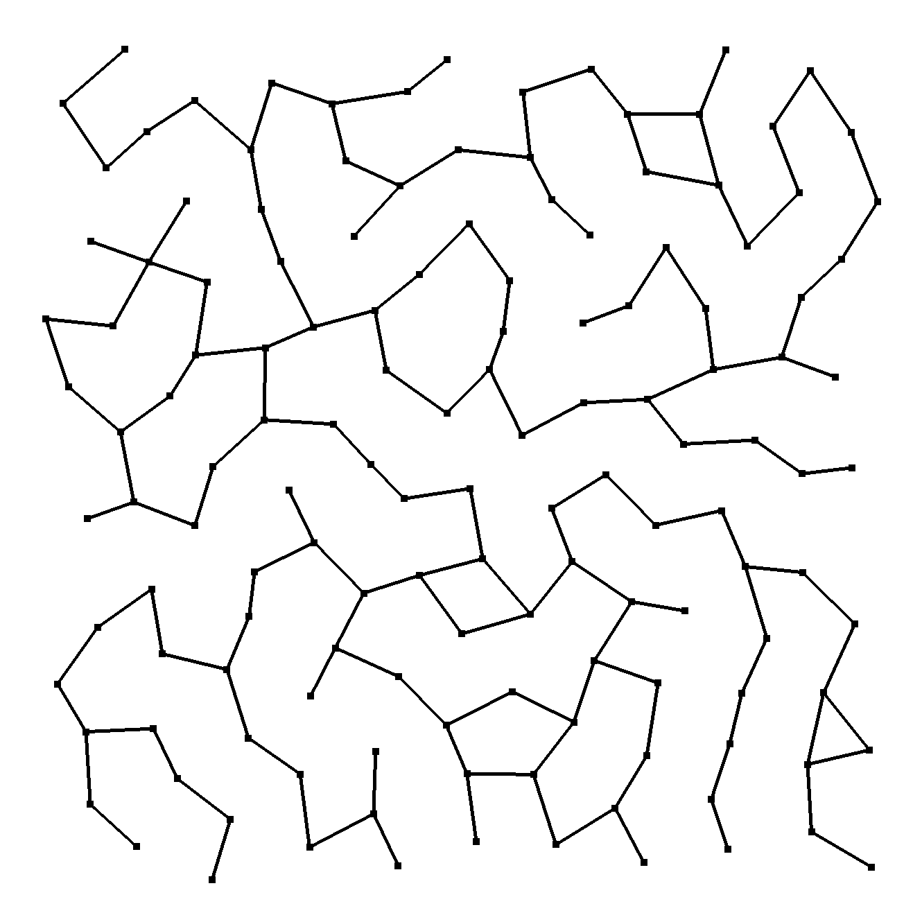
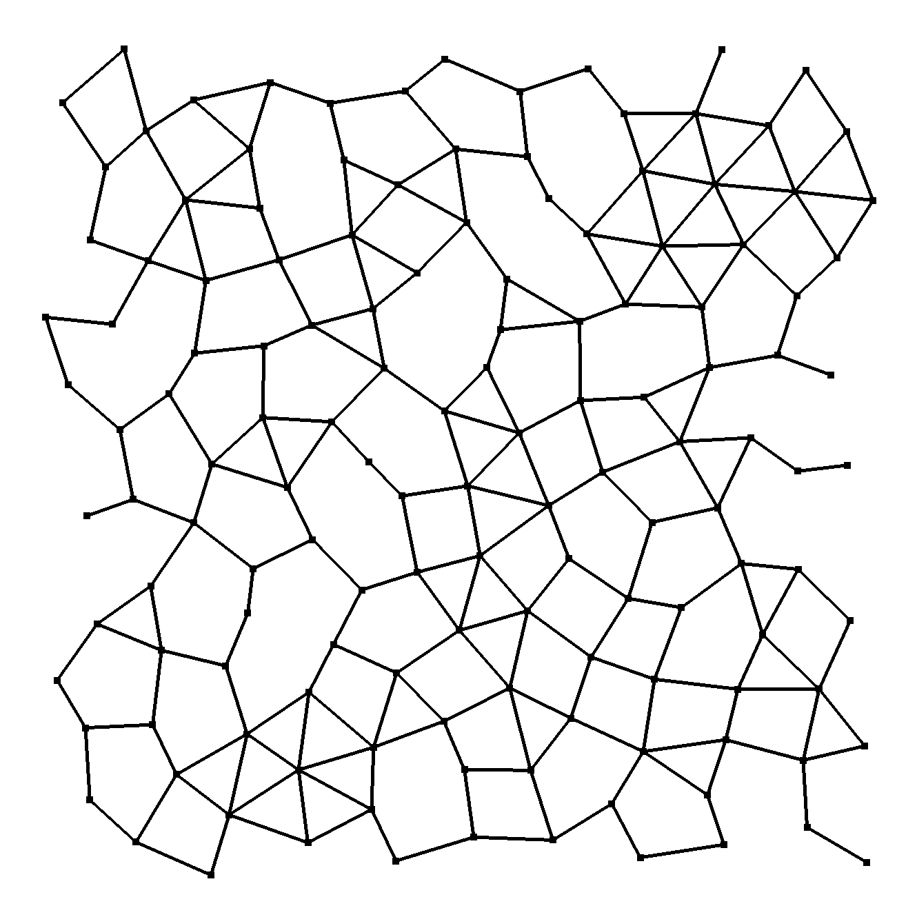
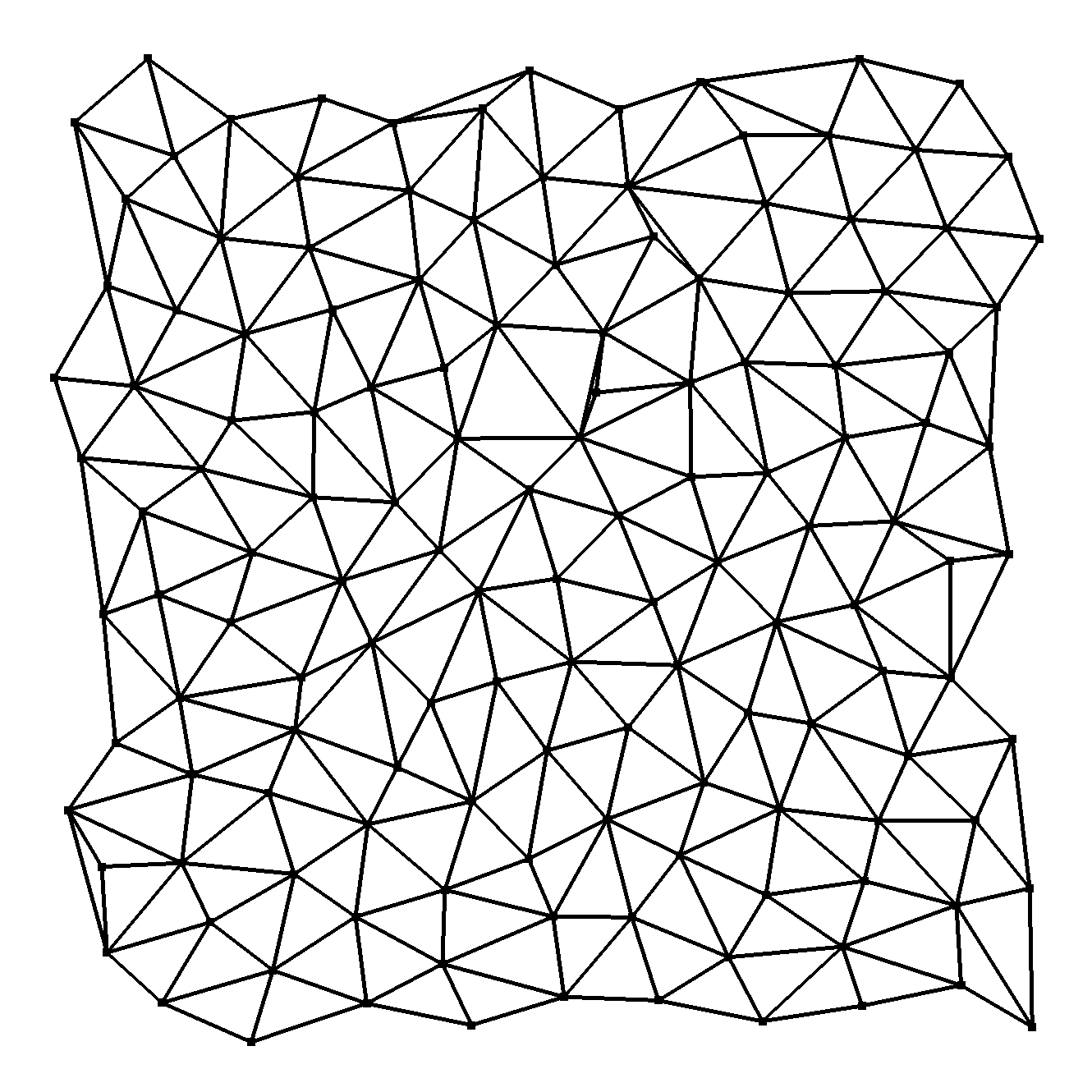
Figure 4. Reconstruction of a 2D point cloud. From left to right, the top row shows the input point cloud, the graph formed by connecting each point to its nearest neighbors within a given radius, and the minimum spanning tree of this graph. The bottom row shows the process of adding edges to the minimum spanning tree. The edges are added in order of increasing length, and edges are only added if they do not violate planarity. From left to right, the bottom row images show the MST with 10, 100, and all possible edges added.

The method to which we allude is based on the simple observation that a tree (in the graph theoretical sense) is always a planar graph, and the planar embedding of a tree is given by a rotation system which defines the clockwise ordering of edges incident on each vertex. Thus, if we have a spanning tree connecting all of our points and an associated rotation system, we effectively have a polygonization with a single polygon whose edges are simply the edges of the tree (with each edge of the tree appearing twice). To obtain a triangle mesh, we recursively insert edges that split polygons into smaller polygons. The process stops when all polygons - except the boundary polygon - are triangles. A simple 2D example is shown in Figure 4 for a synthetic point cloud.

For moderate input sizes and a 2D point cloud, the algorithm outlined above is simple to implement because the points are already embedded in the plane, and the rotation system is given implicitly. On the other hand, when designing an efficient and effective 3D version of the algorithm, we face several challenges. First of all, the rotation system, i.e. the ordering of outgoing edges for each vertex, must be computed consistently for all vertices. Moreover, when connecting points, several geometric considerations are important, and we want to allow connections that violate planarity in order to obtain meshes of arbitrary genus. Finally, efficiency is a concern: when an edge is added, we split a face, and one of the two resulting faces must be relabeled. This is a costly procedure in the initial stages of the algorithm.

In summary, our main contributions are as follows:

• Methodology: A rotation system-based algorithm for triangulating a 3D point cloud by iteratively adding edges to an initial spanning tree. With an explicit outlier classification, all the other inliers are referenced in the output mesh.

• Automatability: An important guarantee that output mesh is always manifold enables reliable automatic workflows.

• Generality: Extending the method to allow the creation of topological handles.

• Controllability: The topology of output mesh can be controlled by the prescribed genus number.

• Efficiency: To make the algorithm efficient, we use a binary tree representation of the edge loops, reducing the cost of relabeling after an edge has been added from linear to logarithmic. Moreover, we add an additional ear clipping process which allows us to avoid relabeling altogether in the later stages of the algorithm.

1.1. Related Work

The vast literature on methods for reconstructing surfaces from points can broadly be divided into methods which interpolate the original points and methods which approximate the point set. The former methods are often combinatorial in the sense that they form meshes whose vertices are the input points, and the latter methods are often volumetric (or implicit), producing a function, $\phi:\mathbb{R}^{3}\rightarrow\mathbb{R}$, which maps points in space to an intensity value or distance to surface. A good example of this type of method is the well known Poisson reconstruction method (Kazhdan et al., 2006; Kazhdan and Hoppe, 2013; Kazhdan et al., 2020) which computes a function, $\phi$, whose gradient field matches the smoothed field of estimated normals for the input points.

Volumetric methods are often simpler to implement than combinatorial, they tend to suppress noise, and they are often good at hole closing. On the other hand, since the original points are not used directly, it is difficult to quantify the remaining noise and, more generally, the precision of the output mesh. For a comprehensive survey, the reader is referred to Berger et al. (2017), and in the following we focus on the most relevant combinatorial methods since our work falls in this category.

The earliest combinatorial reconstruction method appears to be the work of Jean-Daniel Boissonnat (1984). Boissonnat proposes two algorithms, the first of which incrementally grows a polyhedron from a starting edge. The second algorithm is based on removing tetrahedra deemed exterior from the Delaunay tetrahedralization of the point cloud. The mesh resulting from this so-called sculpting process is the boundary of the union of the remaining tetrahedra. Numerous other works, notably the Crust, Power Crust, and CoCone methods of Amenta et al. (Amenta et al., 1998, 2000, 2001) and Edelsbrunner’s Wrap algorithm (Edelsbrunner, 2003) also build on 3D Delaunay tetrahedralization or its dual the Voronoi diagram. We refer the reader to Cazals and Giesen (2004) for an excellent overview. Boltcheva and Levy (2017) proposed a method in which a Voronoi cell is computed for each point and restricted to a disk that is also defined at the same point. Point connectivity can then be inferred from these restricted Voronoi cells. The method requires smoothing for real-world data but it is very efficient and easy to parallelize. More recently, Wang et al. (2022) proposed a method that is likewise based on restricted Delaunay tetrahedralization but restricts to a sequence of globally defined surfaces that approach the final output. This method appears to be effective and robust to variations in sampling density, but at the cost of making a sequence of tetrahedralizations.

Bernardini et al. (1999) proposed the method known as ball-pivoting algorithm (BPA). This method is reminiscent of Boissonnat’s first method as it also grows the mesh a vertex at a time. The BPA starts from a seed triangle and uses the heuristic of pivoting a ball around an edge until it touches the next point, thereby defining a new triangle. In the presence of noise, BPA has a tendency to leave isolated points which are not touched by the rolling ball. A solution proposed by Digne et al. (2011) is to use a scale space approach where the point cloud is first smoothed and then the BPA is applied to the smoothed point cloud. This yields a reconstruction with far more of the input points, and the original vertex positions are stored and used in the final mesh.

Typically, learning based methods for surface reconstruction are volumetric in nature, but combinatorial methods exist. Notably, Sharp and Ovsjanikov (2020) proposed a method which uses neural networks to iteratively propose new triangles and decide whether to include them in the output mesh. Another recent strategy employed by Sulzer et al. (2021) is to start from a Delaunay tetrahedralization and use a learning-based method to classify tetrahedra as being inside or outside. For a recent, quite broad survey of deep-learning-based surface reconstruction, the reader is referred to (Farshian et al., 2023).

Not all combinatorial methods strive to include most points. A method which was expressly designed not to preserve all points was recently proposed by Zhao et al. (2023). In this work quadric error metrics are used to cluster points such that cluster representatives lie at corners and on sharp features. The mesh is then the quotient graph with respect to this clustering.

The approach that is most similar to ours is the work by Robert Mencl (1995) which was later extend by Mencl and Müller (1998). Their starting point is also a minimum spanning tree, but in their case the Euclidean MST is employed whereas we use the MST of a k-nearest neighbor graph. Mencl and Müller also connect vertices and ultimately triangulate the graph, but they do not store the faces of the graph and cannot check if vertices that are connected belong to the same face. This makes it unclear whether it is feasible to avoid topological errors if the points are noisy. Unfortunately, this issue is not investigated. In later work, the same authors propose an improved method based on the so-called $\beta$ environment graphs rather than minimum spanning tree (Mencl and Müller, 2004). While the improved method is clearly effective, we are concerned that spurious handles can be introduced, especially in the presence of noise.

John Robert Edmonds (1960) showed that for any graph imbued with a cyclic ordering of the incident edges for each vertex, i.e. a rotation system, there is a corresponding, topologically unique polyhedron. In the context of interactive modeling, Akleman and Chen (1999) used rotation systems to design the principles of their doubly linked face list (DLFL) representation for polyhedral shapes. Later, Akleman et al. (2003) presented a DLFL-based system where meshes are built using a minimal set of operators which includes an operator that creates a handle by adding an edge connecting two distinct faces.

2. Mesh Representation

We define a graph, $G$, as the tuple $G=(V,E)$, where $V$ is a set of vertices and $E$ is a set of edges. An edge, $e=\{v,w\}$, where $v,w\in V$ is an unordered pair of vertices. For our purposes, loops where $v$ and $w$ are the same vertex will not be needed, hence $v\neq w$.

The set of halfedges, $H=\{(v,w)\;|\;v,w\in V\wedge\{v,w\}\in E\}$. If there is an edge between vertices $v$ and $w$, then $(v,w)$ and $(w,v)$ both belong to $H$. Thus, halfedges, which are sometimes referred to as darts, are simply the directed versions of edges. If $v$ is the first vertex in a halfedge $(v,w)$, we say that $(v,w)$ is outgoing from $v$.

A polygonal mesh, $M=(V,E,F)$ is an orientable topological polyhedron which we can obtain from a graph by associating a set of faces, $F$, with the graph. As described by Edmonds (Edmonds Jr, 1960), we can obtain the faces by associating a rotation system with the graph. A rotation system assigns cyclic orderings of the halfedges outgoing from $v$ for all $v\in V$. We can define the rotation system in terms of a function $\rho:H\rightarrow H$ which maps an outgoing halfedge, $h=(v,w)$ to the next outgoing halfedge in the cyclic ordering around $v$ as shown in Figure 2. In some cases, a vertex, $v$ has only a single incident edge and then $\rho((v,w))=(v,w)$ where $w$ is the only neighbor of $v$.

In order to define the faces of a mesh in terms of a rotation system, we need the function $\iota:H\rightarrow H$ which inverts the orientation of the halfedge. In other words, if $h=(v,w)$ then $\iota(h)=(w,v)$. This means that $\iota$ is a fixed-point free involution, i.e. $\iota(\iota(h))=h$ and there is no halfedge $h$ left invariant by $\iota$.

A face is defined in terms of the composition $\tau=\rho\circ\iota$. Specifically, the face associated with a halfedge, $h$, is $f_{h}=\{\tau^{n}(h)|n\in\mathbb{N}_{0}\}$ or, in other words, the orbit of $h$ under $\tau$. The set of all faces can now be defined as $F=H/\sim$ where $\sim$ is the equivalence relation defined by $h\sim h^{\prime}$ if and only if $h^{\prime}\in f_{h}$. A corner of a face, $f$, at a vertex, $v$, is given by a pair of outgoing halfedges $h$ and $h^{\prime}$ which are adjacent in the cyclic ordering, i.e. $\rho(h)=h^{\prime}$ and such that $h^{\prime}\in f$. A corner can be split by inserting a new outgoing halfedge between the two adjacent halfedges in the cyclic ordering.

In the same vein as faces can be defined as orbits of $\tau$, we can see edges as the orbits of $\iota$ and vertices (including their one-rings) as the orbits of $\rho$. The actions of $\rho$, $\iota$, and $\tau$ along with their orbits are illustrated in Figure 2.

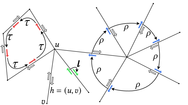
Figure 2. This figure shows a partial graph consisting of vertices, edges, and halfedges (ordered pairs of vertices) indicated as fat arrows. The functions $\rho$, $\iota$, and $\tau=\rho\circ\iota$ map halfedges to halfedges. The thin arrows show the actions of the functions. Orbits of the functions are shown in red (faces), blue (edges), and green (one ring).

2.1. Euler Operators

Editing operations on a manifold mesh, $M=(V,E,F)$, are often defined in terms of the Euler-Poincare formula,

(1) $$|V|-|E|+|F|=2(1-g)\enspace,$$

where $g$ is the genus of the object represented by the mesh. This formula must be satisfied by any closed, manifold mesh. As such, it has been used as an invariant in solid modeling operations as discussed in e.g. (Mantyla and Sulonen, 1982). Typically, operators which maintain the Euler-Poincare formula invariant are called Euler operators. In the following, we will describe the two Euler operators we will need for our surface reconstruction algorithm and how the rotation system of the mesh is affected by these operations. The operators are illustrated in Figure 3.

2.1.1. Splitting a face by edge insertion

A face is split by creating an edge, $e$, between two vertices, $v$ and $w$. Assuming $v$ and $w$ belong to the same face, $f$, this operation splits $f$ into two faces. Thus, it is clear that (1) holds since $|E|$ and $|F|$ both increase by one.

If we define our mesh in terms of a rotation system, the cyclic orderings of outgoing halfedges need to be updated for $v$ and $w$. Moreover, the corners of $v$ and $w$ which are split by the insertion of $(v,w)$ and $(w,v)$, respectively, must both be associated with $f$ for the edge insertion to be valid.

2.1.2. Adding a handle by edge insertion

A topological handle is added by creating an edge, $e$, between a vertex $v$ that belongs to face $f_{1}$ and a vertex $w$ belonging to a different face, $f_{2}$. In this case, $f_{1}$ and $f_{2}$ are merged into a single face which we can see as a tube connecting the holes left by removing $f_{1}$ and $f_{2}$. In other words, this operation adds a handle to the mesh, increasing $g$ by one. (1) still holds since $|E|$ and $|F|$ increase and decrease by one, respectively.

The same caveat applies for handle insertion as for face splitting. At vertex $v$ we need to add the $(v,w)$ halfedge to the cyclic ordering of outgoing halfedges in a corner that belongs to $f_{1}$ and at vertex $w$ we need to add the $(w,v)$ halfedge in a corner that belongs to $f_{2}$.

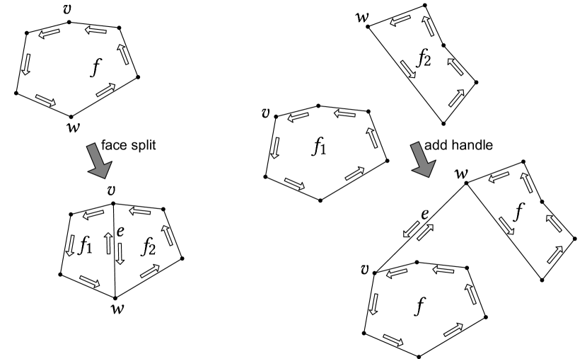
Figure 3. Before (top) and after (below) illustration of the edge insertion operation both in the case (left) where a face $f$ is split into two faces and in the case (right) where two faces, $f_{1}$ and $f_{2}$, are merged into a single face.

3. Method

Our reconstruction method initially forms a tree from the input points and then proceeds to triangulate the tree. The method can be described in terms of three steps, as shown in Figure 1.

1. Initially, we form a graph, $G$, from the input point cloud $V$, $V\subseteq\mathbb{R}^{3}$, by connecting each point to its $k$ nearest neighbors ($k$NN) within a given max radius, $r$. Based on $V$, we estimate the normal by applying principal component analysis (PCA) and correct the orientation through a normal-angle-weighted minimum spanning tree (MST). Afterward, we compute a rotation system (RS) that stores the cyclic ordering of the outgoing edges for each vertex. Based on the $k$NN graph, a distance-weighted MST, $T$, is produced from this graph $G$.

2. Next, to increase the connectivity of $T$, we insert edges from $G$ that connect leaf vertices to other vertices which are potentially far away in terms of graph distance but belong to the same face. Before making a connection, we perform both a topological check and checks of the geometric validity and quality of the connection.

3. Finally, we create the mesh $M$. $M$ is initialized to $T$ augmented with the additional edges. We split triangles from the faces of $M$ by greedily adding edges from $G$ until no more valid triangles can be formed.

In the following, we will describe each of these steps in more detail and then discuss how the algorithm can be generalized to allow for meshes of arbitrary genus.

3.1. Initialization

As stated earlier, the initial graph $G$ is derived from the input point cloud. Vertices are formed from the points, and each vertex is connected to its $k$ nearest neighbors ($k$ and other parameters are listed in Table 1). Based on $G$, two minimum spanning trees, a normal-angle-weighted MST and a distance-weighted MST, are generated for later use.

Unoriented normals are computed using the PCA method, but in order to construct the correct rotation system, we need the normal orientations. These we obtain from the normal-angle-weighted MST. Edges in this MST keep a weight calculated using the normals of involved vertices (Hoppe et al., 1992),

(2) $$w_{u,v}=1-|\mathbf{n}_{u}^{T}\mathbf{n}_{v}|$$

In other words, edges between vertices $u$ and $v$ with small angles between their respective normals have a small weight. Starting from an arbitrary vertex, a consistent normal orientation is propagated to all vertices along the edges of the normal-angle-weighted MST.

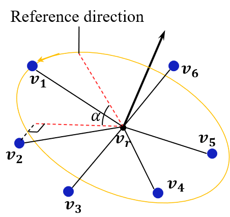
Figure 5. RS of an example neighborhood. Taking $v_{2}$ as an example, it is projected on the disk and then an angle $\alpha$ is calculated as the radian of vertex $v_{2}$.

The distance-weighted MST, $T$, is used as the initial structure of the mesh. It is generated based on the Euclidean distance as the edge weight. At the same time, we build the rotation system (RS) which determines the cyclic ordering of the neighbors of all vertices. As shown in Figure 5, every neighbor of $p_{r}$ is projected onto its tangent plane (based on the oriented normals). Starting from a given (but arbitrary) reference direction, the angles of neighbors are calculated, and a cyclic ordering is computed by sorting the neighbors according to these angles. Effectively, this produces the $\rho$ operator. The RS is computed on the original graph $G$, but not all edges are a part of $T$. Given an halfedge, $h\in T$, $\rho(h)$ yields the next halfedge in the cyclic ordering of outgoing halfedges belonging to $G\cap T$. As $T$ is updated by inserting edges from $G$, so is the $\rho$ operator.

3.2. Edge insertion

Before triangulating the MST $T$ to form a mesh, an edge insertion step is needed to increase the connectivity of $T$.

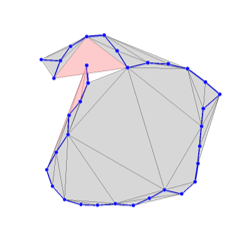
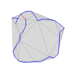
Figure 6. An example showing the necessity of edge insertion. The left figure presents the position of input 2D points. The reconstruction result in the middle is generated without edge insertion, where the blue lines are the MST. The figure on the right depicts an ideal reconstruction result. This is achieved by the edge insertion before triangulation, the red edge in this plot.

While the MST is a planar graph by virtue of being a tree, directly proceeding to triangulation generally leads to a poor result where ill-shaped and self-intersecting triangles are formed. Figure 6 illustrates why this can happen. A 3D illustration on Stanford Armadillo is shown in Figure 7. The lack of connectivity of $T$ leads to overlapping geometry in this example. Compared with the triangulation stage, edge insertion is more time-consuming with both topology and geometry tests. Hence, establishing possible connections on all leaf nodes emerges as a viable strategy, ensuring ample connectivity within a reasonable execution timeframe.

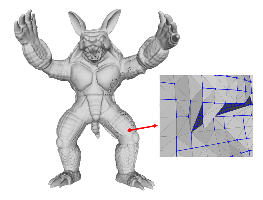
Figure 7. A 3D example of triangulation without edge insertion, where the blue edges are the MST. A random origin of the crack is zoomed in, which is caused by the limited connectivity of $T$.

For every leaf node, we take its $k/2$ nearest neighbors as connection candidates. The closest candidate passing specific tests will be connected.

Two mandatory tests are employed on all leaf nodes considered as end-points for new edges. The first is a topological test, which ensures that the edge insertion does not change the topology of $T$ that should remain planar (although we relax this constraint later). The second is a geometry test, which ensures that the edge insertion does not lead to self-intersecting triangles.

In practice, we also use a quality test to avoid geometrically poor configurations. Also, the quality check increases efficiency by rejecting invalid edges via more lightweight checks. More details will be introduced in Section  4.2.1.

3.2.1. Topology Test

As mentioned, a face in a graph is defined as an orbit, i.e. the set of edges obtained by repeated application of $\tau$. The topology of the graph will not change as long as inserted edges only split faces rather than connecting different faces. Examples can be found in Sec. 5.1. From a practical point of view, we store an identifier of the associated face with each halfedge. These identifiers are stored in a tree structure for efficiency concerns (for more information, please refer to Sec. 4.3). For a candidate edge, $\{u,v\}$ we check both that $u$ and $v$ belong to the same face, $f$, and also that when $(u,v)$ is inserted in the cyclic ordering of outgoing edges at $u$ and $(v,u)$ in the corresponding ordering at $v$, the corners that are split also belong to $f$ as mentioned in Sec. 2.1.1.

3.2.2. Geometry Test

The geometry test inspects the local geometry around a given vertex within the tangent plane to avoid self-intersecting or overlapping triangles. As illustrated in Figure 8, two point sets, a query set and a rejection set, are retrieved based on Euclidean distance. Each existing edge in the rejection set, such as edge $e$ in the figure, will be used to reject candidate connections if intersections occur. The radius of the rejection set should be large enough to include all possible rejection edges. Thus, it is calculated with (3), where $r_{\mathrm{qry}}$ stands for the radius of the query set while $L_{\mathrm{max}}$ represents the maximal existing edge length.

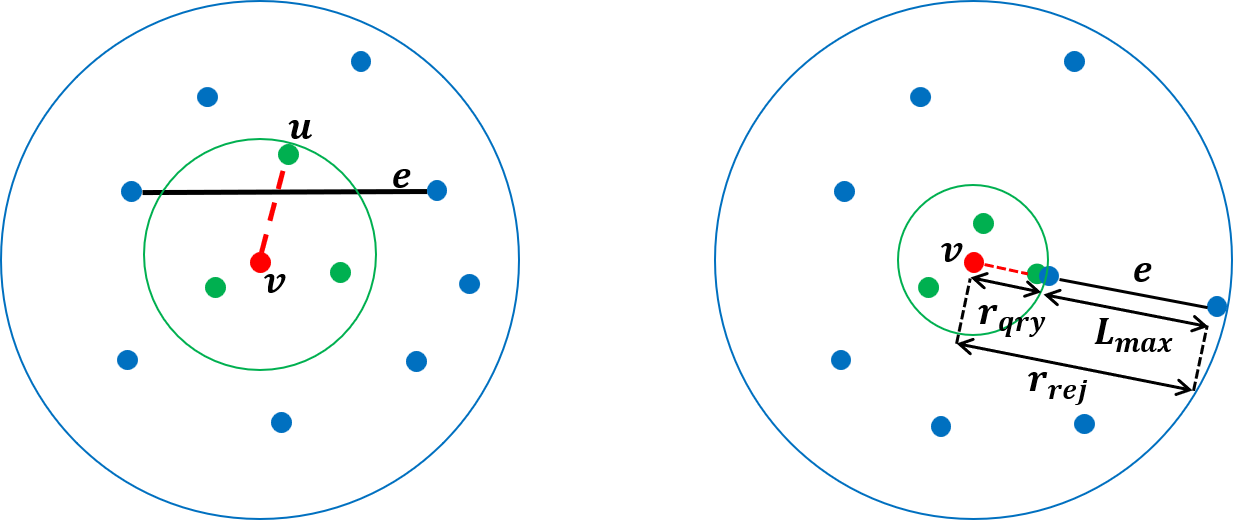
Figure 8. A geometry test applied to vertex v. The green points are the query set and the blue points together with the green points are the rejection set. The red dashed line represents the candidate edge insertion and the black edge e is an existing edge. In the left case, the candidate end vertex u will be rejected because of the existence of e. The right configuration shows the extreme situation where the radius of the rejection set reaches the maximum.

(3) $$r_{\mathrm{rej}}=r_{\mathrm{qry}}+L_{\mathrm{max}}$$

When extending this check to 3D, an additional requirement about vertex normal orientation on the query/rejection set selection is applied, to deal with thin structures or areas with high curvature. If a vertex $u$ and root $v$, with normal $\mathbf{n}_{u}$ and $\mathbf{n}_{v}$, have a negative inner product on normal, i.e. $\mathbf{n}_{u}\cdot\mathbf{n}_{v}<0$, then vertex $u$ is not included in either point set.

3.3. Triangulation

When edge insertion has completed, we initialize the output mesh, $M$ to be a copy of $T$. We then proceed to triangulate $M$ by greedily adding edges from $G$ to $M$ until no more triangles can be formed.

The first step of triangulation is to compute the set of potential edges which could be added. We start by visiting all vertices of $M$, and for each vertex, $v$, we consider all outgoing halfedges. For each outgoing halfedge, $h_{1}=(v,u)$, we use the $\rho$ operator to find the next halfedge, $h_{2}=(v,w)$ and then the incident vertex, $w$, to which it points ($h_{1},h_{2}\in T$). Our edge candidate is now ${u,w}$. All edge candidates are pushed onto a priority queue, $q_{h}$, where the Euclidean length of prospective edges is the priority.

In each iteration of the triangulation loop, we pop an edge candidate to form a triangle if the edge passes the validity check which ensures both good topology and geometry. The validity check has three steps:

• We check that the inserted edge (shown dashed in Figure 9) does not violate the RS. We check this by ensuring that the edges of the triangle are indeed adjacent in the cyclic ordering of all three vertices after the edge has been inserted. With reference to Figure 9 this means that $h_{1}=\rho(h_{2})\wedge h_{4}=\rho(h_{3})\wedge h_{6}=\rho(h_{5})$, where we also require that $\alpha<\pi\wedge\beta<\pi\wedge\gamma<\pi$. Without the angle constraint, flipped faces would be valid.

• A heuristic face overlap check is performed to avoid the main cause of cracks in practice. For a triangle face, $f=(v,u,w)$, we project all vertices in the union of its $k$ nearest neighbors to the plane where the face lies, based on the face normal. If any of the vertices lies inside the triangle, the candidate is rejected. This approach serves as an effective method for preventing intersections and acts as a safeguard against undesirable configurations in which edge insertion is not feasible.

If the edge is valid, we update its halfedges with a new face identifier and insert its halfedges in the rotation system of $M$.

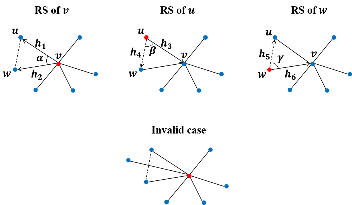
Figure 9. Illustration of RS inspections. The bottom row gives an invalid case. The dashed line corresponds to the edge considered for connection.

3.4. Reconstructing high genus meshes

As described above, this method can only reconstruct meshes of sphere or disk topology since no connections are made which could change the topology of the mesh. In order to facilitate reconstruction of objects with higher genus, we make a very simple adjustment to the algorithm.

As the pipeline in Figure 1 illustrates, for high-genus shape, two more operations called conservative triangulation and handle connection are required. The only difference between conservative triangulation and normal triangulation is that there is a threshold for edge length in conservative triangulation. This threshold is different for each vertex. It is implicitly encoded with the longest connection involving each vertex in the initial graph $G$. For instance, if a vertex $v$ has $k$ connected neighbors in $G$, the conservative edge length threshold of $v$ is determined by the length of the $2/3\cdot k$-th shortest edge associated with $v$. The reason for using a conservative triangulation step is that we thereby avoid skinny triangles encroaching on faces that are likely to be end-points of handles in the next step. Since a final triangulation stage follows handle insertion, we can afford to be conservative in the first step.

After undergoing conservative triangulation, the mesh $M$ attains a state where the majority of potential connections have been established. Assuming local edges share an average edge length $\overline{|e|}$, at this stage, an expected handle $\{u,w\}$ possesses a characteristic distinct from those of spurious handles: $d_{g}(u,w)\cdot\overline{|e|}\gg\overline{|e|}$, where $d_{g}$ is the graph distance. In practice, we use $d_{g}(u,w)>2n$ to detect if it is a handle we would like to connect.

To insert handles, we consider all edges of $G$ which have not been inserted in $M$ and whose end-points belong to different faces. If the edge fulfills the above condition, we enqueue it for insertion. Once all candidates have been considered, we insert the edges. The operation is exactly the same as the previous edge insertion except that when adding handles we only connect vertices which belong to different faces.

3.5. Dealing with noisy data

Scanned point clouds are always noisy since the points are based on measurements that are inherently subject to noise. Moreover, when we reconstruct from point clouds, we typically combine several sub-scans. These may not be perfectly aligned, introducing another source of noise.

Noise can be both tangential and normal to the surface. While tangential noise does not affect the reconstruction, normal noise can result in large Euclidean distances between points that are quite close in the tangent plane. To mitigate this issue, we use the estimated normals to project the points onto the tangent planes and compute the projected distances rather than the Euclidean distances.

To define projection distance, we need some preliminary definition: for edge $e=(v,u)$, $e_{//v}$ refers to the projection of $e$ on the tangential plane of $v$. The projection distance $|e|_{p}$ is defined

(4) $$|e|_{p}=(|e_{//v}|+|e_{//u}|)/2\enspace.$$

This approach enables the acquisition of a more noise resilient MST as the initial structure for reconstruction. However, an important consideration arises: when calling kd-tree in Euclidean distance at the initialization stage, it is conceivable for the initial graph $G$ to lack a valid connection between two vertices, even when the projection distance is small but the Euclidean distance is substantial due to noise. To mitigate this issue, a new kd-tree containing projected vertices is established and employed for all nearest-neighbor searches right from the outset.

4. Implementation

In this section, we discuss the practical aspects of the method in the order of the pipeline outlined in Section 3. These aspects include details of the quality test used in edge insertion, the binary tree data structure used to maintain faces, and the parameters used in the method.

4.1. Initialization

In the initialization phase, we construct a rotation system RS associated with the graph $G$. From a theoretical point of view, the RS is simply a cyclic ordering of neighboring vertices for each vertex of $G$, and the topology of the reconstructed surface is not dependent on which cyclic ordering we choose for each vertex. However, the geometry may become very convoluted if the cyclic orderings of two adjacent vertices are geometrically inconsistent.

Intuitively, geometric consistency means that if vertex $u$ is left of $v$ then $v$ must be right of $u$. Unfortunately, if we are dealing with a noisy point cloud and $u$ and $v$ are extremely close vertices in the sense of projection distance, small variations in the vertex normals can cause the cyclic orderings to be inconsistent. Typically in the example case depicted by Fig. 10, two vertices $u$ and $v$ possess an extremely short projection distance, a slight normal difference caused a situation that: both of them think they are at the top-left side of the other one. The neighbors of $u$ and $v$ are in the same order in the cyclic ordering of both vertices, e.g. given three neighbors $a$, $b$, and $c$, we have

• neighbors of $u$: $[a,b,c,v]$, and

• neighbors of $v$: $[a,b,c,u]$.

Since $u$ and $v$ have the same position in each other’s cyclic ordering, each is, effectively, top-left of the other. This is a problem from a geometric point of view since no straight edge can connect $u$ and $v$ consistently in this case. The situtation would lead to very convoluted faces.

In practice, the issue arises more often when the edge between two vertices is almost colinear with the normals of the vertices. Consequently, if the angle between the edge and the mean normal of the incident vertices is below a specified threshold $\phi$, the normal of one vertex is assigned to the other. This adjustment reduces the situation to the 2D case locally and ensures that there is a consistent connection between the two vertices.

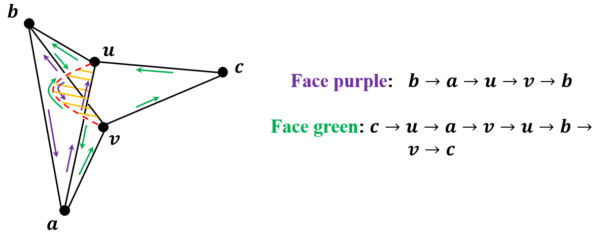
Figure 10. The consequence of RS inconsistency. Note that the assumption here is that $u,v$ are extremely close to each other in 2D plane, this figure shows the rotation system of $u$. The rotation system will be the same for $v$ except for the swapped positions of $u$ and $v$. If the connection $\{u,v\}$ is allowed, convoluted faces will be created at the region of the orange shadow.

4.1.1. Analysis

The initialization includes construction of a 3D kD-tree, computation of an MST, and initialization of the rotation system. Construction of such a kD-tree can be done in $O(N_{v}\log N_{v})$. With the kD-tree constructed, we generate a $k$NN graph by use of $k$NN queries on the tree. In the worst case, each query takes $O(N_{v})$ time to answer, but for practical purposes the expected running time of each query is $O(\log N_{v})$(Friedman et al., 1977). We can then compute the MST with an algorithm such as Prim’s algorithm in $O(kN_{v}\log N_{v})$ time. Finally we traverse the MST, constructing the rotation system by ordering of neighbours around each vertex.

The worst case total time for initialization is thus $O(N_{v}^{2})$, due to the pessimistic bounds on answering $k$NN queries. For non-adversarial input, one would expect $O(kN_{v}\log N_{v})$ time.

4.2. Edge insertion

During the edge insertion stage, two tests are formulated to ascertain the soundness of both topology and geometry. Nevertheless, extensive experiments have revealed that the quality of connections established during this stage is pivotal in preventing holes, even though they are both topologically and geometrically closable. Consequently, a third practical test called the quality test, is implemented to uphold the connection’s high quality and align with intuitive expectations. Additionally, for enhanced efficiency, we have introduced a replacement setting for the geometry test.

4.2.1. Quality Test

In this test, several heuristics are employed to ensure the quality of the connections, as depicted in Fig. 11.

• Firstly, an angle threshold, $\theta$, is imposed on the edge to which the leaf vertex $v$ is connected: $\alpha\geq\theta\wedge\beta\geq\theta$. This threshold ensures that we do not create extremely skinny triangles.

• Next, we require that the normals of $v$ and the prospective connected vertex have a positive inner product, i.e. $\mathbf{n}_{v}\cdot\mathbf{n}_{u}>0$. This rule is needed to ensure that we do not make connections between opposite sides of thin structures.

• Also, as we mentioned in Sec. 4.1, we want to avoid as many cases of inconsistency as possible. A solid inconsistency check is applied here: for any possible RS-valid triangles incident to this candidate, if the normals of three vertices point at the same side, it is consistent. Otherwise, any inconsistent case will get the candidate rejected.

• Lastly, an angle threshold of $\gamma>90^{\circ}$ is imposed on the angle between the edge from $v$ to its parent vertex and the edge from parent to either grandparent or sibling. This helps ensure that we do not make connections to vertices that are too close in terms of graph distance. We avoid such connections since only a single connection is made from leaf vertices, and short connections are made in the triangulation phase.

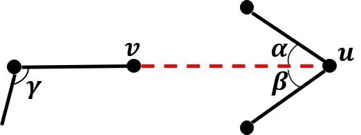
Figure 11. An example configuration supporting the explanation of the quality test. The red dashed line is the connection to be considered.

4.2.2. Geometry test

In practice, considering efficiency, we use a fixed number $k/2$ of nearest neighbor vertices as the query set. At the same time, we pick a rejection set of $n\cdot k/2$ nearest neighbors to ensure that $r_{\mathrm{rej}}\gg r_{\mathrm{qry}}$. It turns out that this setting is more suitable considering both local point density and efficiency.

4.2.3. Analysis

The running time of the edge insertion stage is dominated by the knn queries used to inspect the local geometry. Recall that we have constructed a kD-tree of the input points, and that a pessimistic worst case bound on answering these queries is $O(N_{v})$. Recall also that this edge insertion is applied to all leaves of the MST. It follows then that there are at most $O(N_{v})$ leaves to consider, each incurring $O(N_{v})$ worst case costs, totalling in $O(N_{v})^{2}$ time spent. In practice, the number of leaves might be much smaller, and the time to answer knn queries might behave closer to $O(\log N_{v})$.

4.3. Maintaining Faces

In order to efficiently perform the topology test described in Section 3.2.1, we need a data structure that allows us to quickly determine if two half-edges lie on the boundary of the same face, while also supporting fast updates as edges are inserted and faces split.

Using the Euler Tour technique (Henzinger and King, 1999), we store the sequence of half-edges of each face in a balanced binary tree with implicit keys. To query if two half-edges lie on the same face, we can simply traverse to the roots of the associated binary trees and compare, allowing for $O(\log N_{v})$ queries.

Storing the faces in this manner also allows for the use of standard binary tree operations, such as splits and joins, to be used in $O(\log N_{v})$ time. When inserting a new edge, we perform at most two splits to obtain binary trees representing the sequences of half-edges that bound the newly split face, and at most three joins to incorporate the new half-edges in these sequences. Thus, we can maintain the faces under insertion of new edges in $O(\log N_{v})$ time as well.

4.4. Triangulation

During triangulation, besides connecting edges, we need to generate the triangles incident to the connected edges. A common situation is that multiple possible triangles are incident to the candidate connection $\{u,v\}$. Fig. 12 illustrates a typical example where the red dashed line is the candidate connection. We iterate all the third vertex of the incident triangles other than $u$ and $v$. There will only be at most one triangle keeping a valid RS shown in Figure 9 for $h=(u,v)$. Similarly, for $h=(v,u)$, at most one triangle exists with valid RS. Thus, we can keep the 2-manifold of the output mesh and, at the same time, generate all valid triangles without leaving holes.

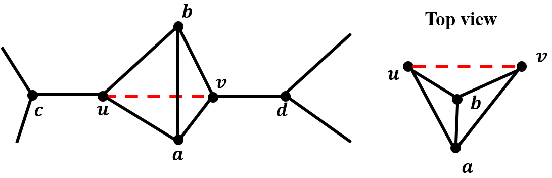
Figure 12. An example when a connection can trigger the generation of multiple triangles. The RS check will filter out all the invalid triangles and keep the 2-manifold property.

To perform triangulation, a bound on the worst case number of candidate edges is $O(kN_{v})$, since for each outgoing edge of each vertex we add exactly one candidate. We construct a priority queue on these candidate edges, perform our validity check, and potentially add them to our structures. The total cost per edge is then $O(\log N_{v})$, totaling in $O(kN_{v}\log N_{v})$ time to triangulate.

To check the distance criteria when reconstructing higher genus meshes, we run a restricted Dijkstra’s algorithm that stops early if the criteria has been met. Note that the number of edges in the graph is upper bounded by $O(kN_{v})$, since we are triangulating a subset of a $k$NN graph. Our worst case bound for this restricted search is thus $O(kN_{v}\log N_{v})$, attributed to the fact that we might not reach the early stopping condition, before the entire graph is explored.

Recall that the candidate edges for handle insertion are obtained from the $k$NN graph. There are thus $O(kN_{v})$ candidates in the worst case. Recall then that the criteria for insertion is that the distance along the graph between two endpoints of a candidate edge is longer than the euclidean distance. Thus, since adding edges to the graph cannot increase the distance along the graph, we need only examine each candidate once in order to either add it, or disqualify it from all future examinations.

Therefore we perform these restricted Dijkstra searches at most $O(kN_{v})$ times, totalling in $O(k^{2}N_{v}^{2}\log N_{v})$ time in the worst case.

As we run the algorithm for $k=30$, the total running time becomes $O(N_{v}^{2}\log N_{v})$ in the worst case.

4.5. Parameter settings

In Section 3 and Section 4, several parameters need to be set. Table  1 shows all the settings used in our implementation. While the settings were arrived at experimentally, the trade-offs between performance and efficiency are clear and explained in the following.

Variable name	$k$	$n$	$\theta$	$\phi$
Value	30	5	30	10

Table 1. Practical parameter settings in the implementation.

The variable $k$ denotes the connectivity of the local neighborhood in the initial graph $G$. For optimal performance, creating a complete graph from the input point cloud is ideal, ensuring all potential edges are considered. However, achieving both time and memory efficiency in such a scenario is impractical. Therefore, under feasible conditions for running time and memory usage, a larger value of $k$ minimizes the likelihood of missing valid connections. Simultaneously, $n$ serves as a multiplier to establish a $\gg$ relationship; as $n$ increases, the result becomes more reliable. However, a trade-off exists, as larger values of $n$ lead to longer running times.

The parameters $\phi$ and $\theta$ represent angle thresholds for detecting inconsistency and measuring connection quality. An excessively large $\phi$ poses the risk of introducing new inconsistencies into the neighborhood, while an overly large $\theta$ can eliminate potentially good connections, causing consequences as illustrated in Figure 6.

5. Results

In this section, we first discuss an ablation study we conducted to provide an understanding of the tests in Section 3.2.

To evaluate our method extensively, we carry out experiments on two different types of point cloud, specifically from synthetic data, i.e. data sampled from existing surfaces, and real scanning data. For the synthetic data sets, we assume that they are sampled sufficiently densely to admit an unambiguous reconstruction and that they are not strongly affected by noise.

On the other hand, the real scans are often more dense since they tend to be composed of several combined scans. This makes it easy to estimate a relatively smooth normal field despite this type of data typically being affected by significant amounts of noise.

We will compare our reconstructions to state-of-the-art combinatorial reconstruction methods and screened Poisson reconstruction. All the experiments were conducted on a laptop with a CPU 11th Gen Intel(R) Core(TM) i7-11800H @ 2.3GHz and 16 GB RAM.

5.1. Ablation study

As delineated in Section 3.2, the edge insertion stage involves three separate tests: the topology test $T_{t}$, the geometry test $T_{g}$, and the quality test $T_{q}$. To assess the importance of each test, we conducted an ablation study. In the baseline configuration all three tests are active. Generally, if we insert an edge that is undesirable, the consequence is that it prevents further insertion, leading to holes. Hence, the quantitative metric adopted is the count of boundary edges ($Bdry.e$). The raw range data of the Stanford Bunny is chosen as the test input due to its widespread recognition and its capacity to expose challenges encountered during edge insertion in our algorithm.

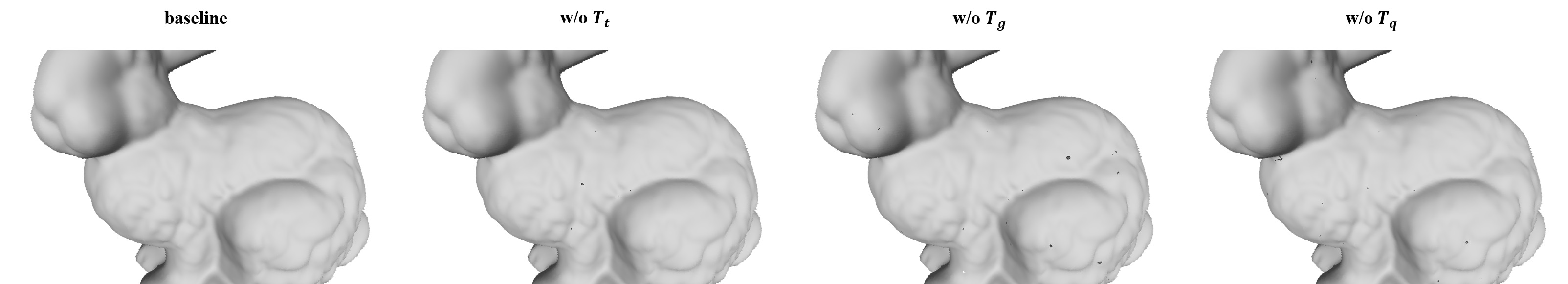
Figure 21. Qualitative result of the ablation study. With all three tests on, the reconstructed bunny has exactly 8 holes around the bottom due to the missing data. With any of the three tests off, more small holes exist than the baseline result.

Figure 21 depicts the qualitative results, while Table 2 presents the quantitative results. Below, we analyze our findings and provide zoomed-in examples from each experimental setting.

Table 2. Statistics of ablation study. A larger number of boundary edges are left when any of the three tests are switched off, which means holes exist.

Experiment setting	baseline	w/o $T_{t}$	w/o $T_{g}$	w/o $T_{q}$
$Bdry.e$	173	385	889	720

W/o topology test

Fig. 13 depicts a typical type of failure when the topology test is off. The red triangle in each picture connects two boundary edge loops. Effectively, this means that a spurious handle is introduced.

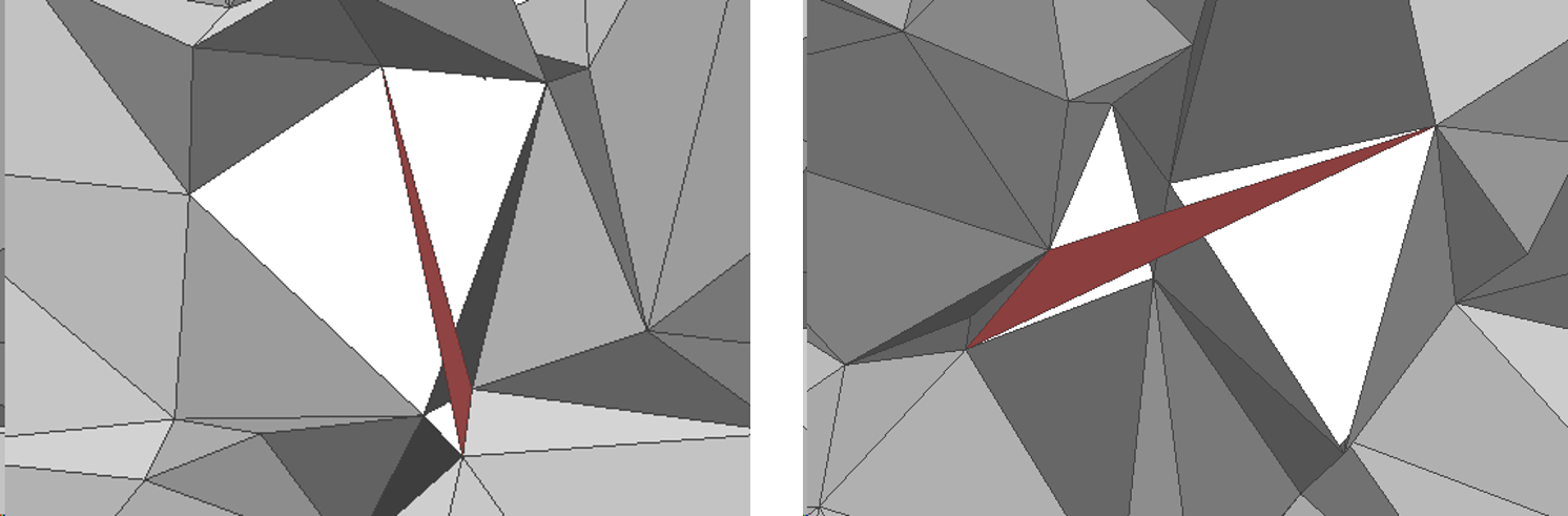
Figure 13. Failure cases when the topology test is switched off.

W/o geometry test

Fig. 14 illustrates a failure case occurring when the geometry test is disabled. All the holes remaining on the bunny exhibit a consistent type of configuration, referred to as a ”candy wrap” or ”twisted connection”. These are deemed highly undesirable from a geometry point of view, despite not being a topological problem. The geometry test serves to reject instances of the candy wraps.

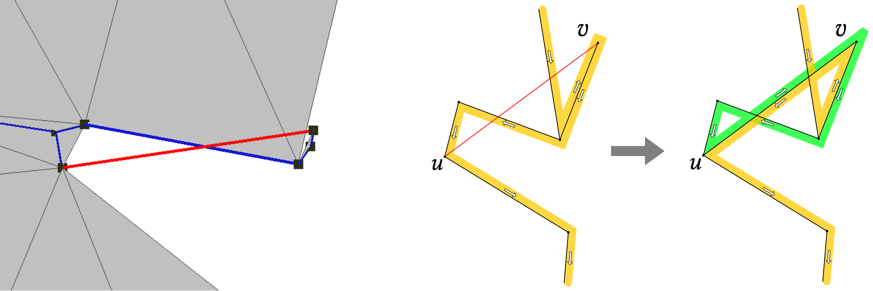
a                                         b

Figure 14. Failure case when the geometry test is switched off. (a) shows part of a reconstructed mesh where the red edge is rejected by the geometry test. (b) shows the abstraction of this configuration from which we can see that the topology test would not reject the red edge, but if it is added we get faces (indicated by fat green and yellow lines) that are twisted in a fashion similar to candy wrapping.

W/o quality test

Fig. 15 demonstrates a failed example after switching off the quality test. If we construe the mesh and the surrounding hole as an ”island” and a ”lake” connected by a thin bridge, the issue is that due to a connection in the bridge made possible by disabling the quality check, the boundaries of the lake and the island are edge loops with different face ID’s. Hence, they will not be connected although they clearly belong to the same surface component.

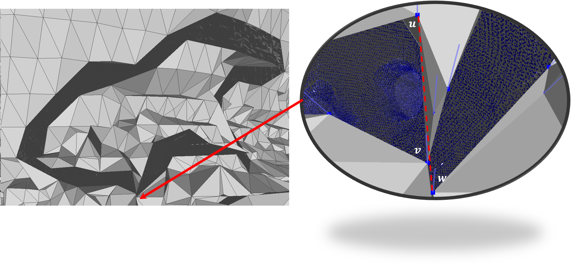
Figure 15. Failure case when the quality test is switched off. The connection $\{u,w\}$ represented by the dashed line causes the boundary loop of mesh fragment inside the hole to become independent of the outer boundary loop. Hence, no connections are made between them.

5.2. Synthetic datasets

In this section, we will present the reconstruction of synthetic point clouds.

5.2.1. Stanford 3D Scanning Repository

In this test, we use the vertex positions and normals from the reconstructions (Curless and Levoy, 1996) provided by Stanford Computer Graphics Laboratory.

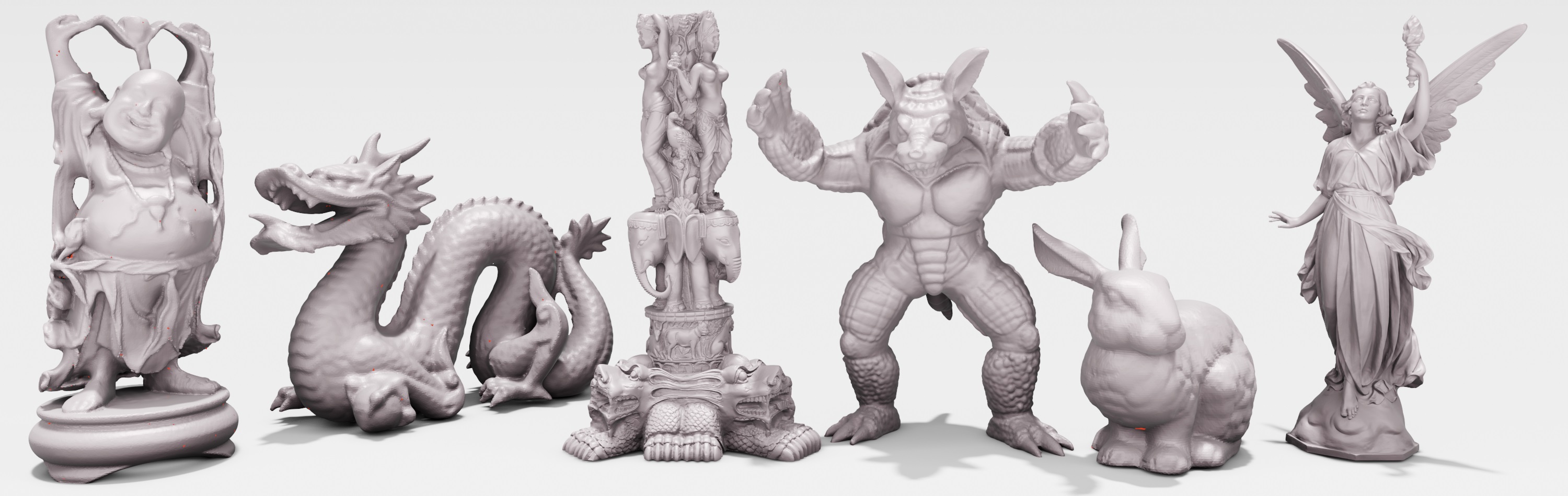
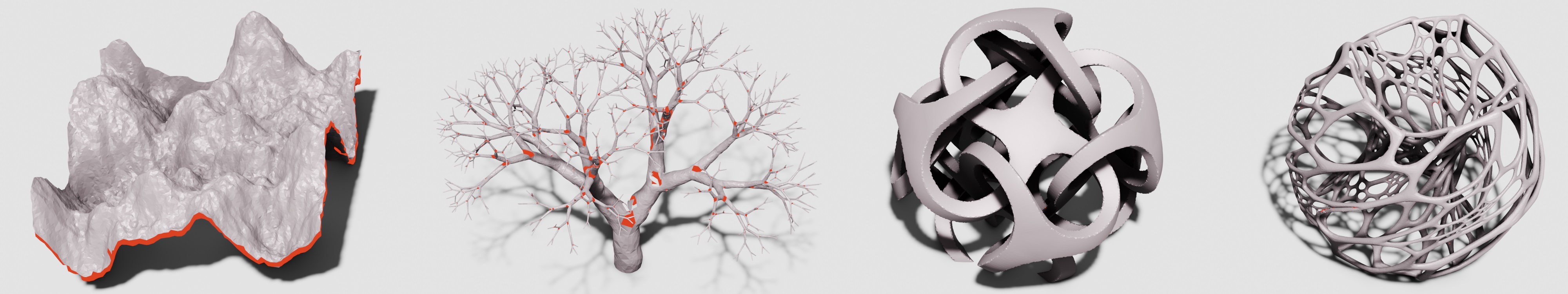
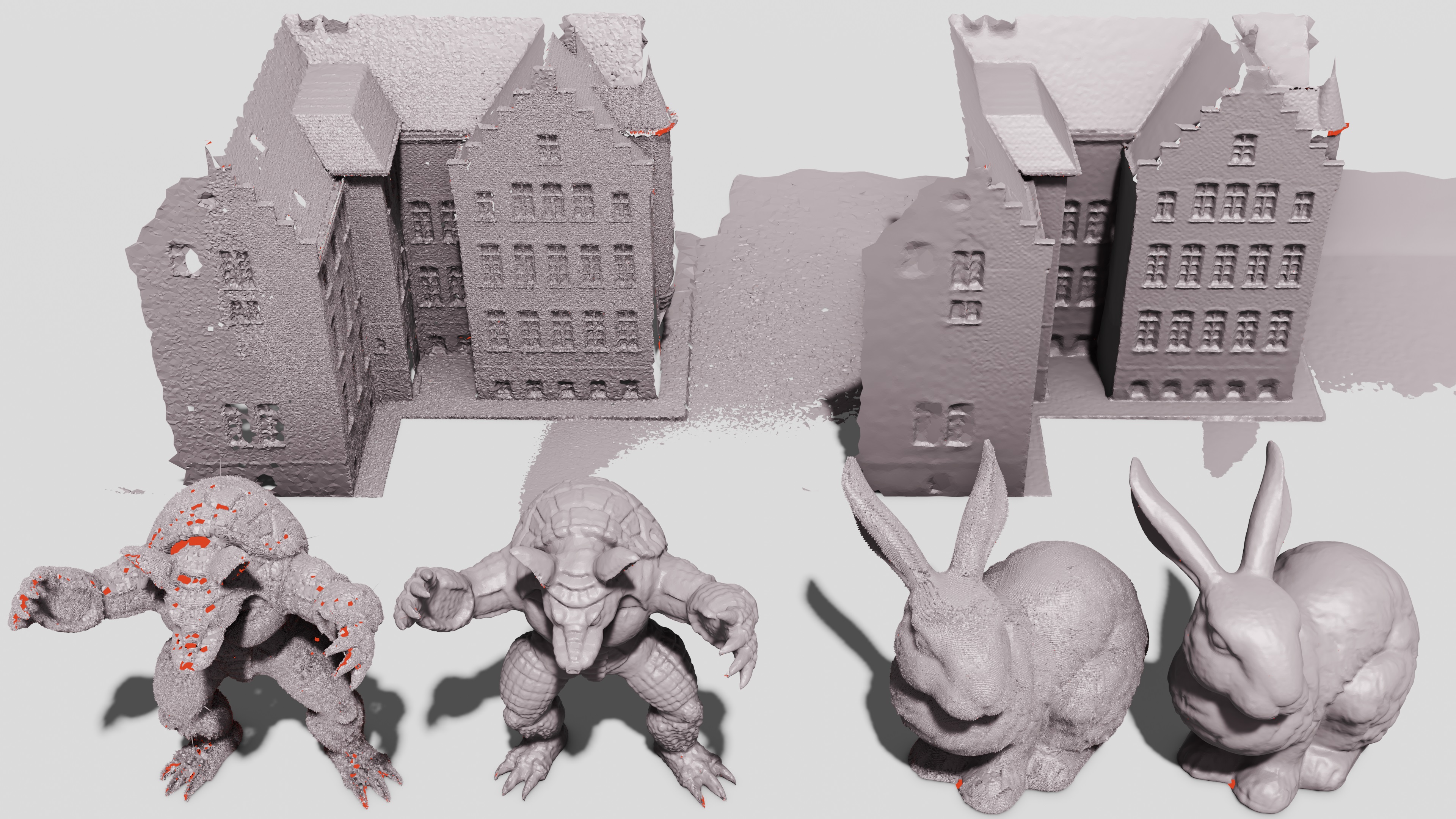
Figure 16. Renderings of models reconstructed using our method. Top image: well-known models from the Stanford 3D Scanning Repository. Middle image: several test objects are shown. The terrain (shown after hole closing) consists of two very close surfaces, the tree exhibits significant variation point density, and the two remaining objects are high-genus shapes. Bottom: we used our method to reconstruct the DTU STL0024 model as well as the Stanford Armadillo and Bunny directly from the acquired points. For each model, we see unprocessed reconstructions on the left and models after hole closing and denoising on the right. In all images, back facing surfaces are rendered in red to show holes in the reconstruction.

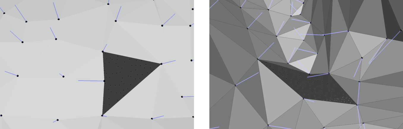
Figure 17. Examples of holes in the reconstruction result on Stanford repository. The short blue lines specify the normal direction of each vertex. The left image gives the example of a hole happening on both Dragon and Happy Buddha due to bad input normal direction. Meanwhile, the right image shows the only hole on Armadillo due to an intense normal change (too sparse sampling).

Figure 16 (top) offers a qualitative demonstration of our reconstruction. All meshes are free from face intersections without considering areas with ill input. At the same time, only a few holes exist because of bad normal input (Dragon, Happy Buddha) or too sparse sampling density (Armadillo). Examples are given in Figure 17.

Table 3 illustrates practical information about reconstructing these meshes, including the number of input vertices ($\#.v$), running time ($t(s)$), and the number of output faces ($\#.f$). One can notice that the time consumption increases almost linearly with the number of vertices in the input except for Lucy. The reason why Lucy takes much longer time to finish is that it takes too much memory and hits the paging / virtual memory mechanism, which requires a lot of data transfer with disk memory. The upper bound of the input point cloud size with normal execution can be estimated. Under current hardware conditions, the maximum input size that can be processed within a linear time growth range is approximately 10M points.

Table 3. Practical statistics of reconstruction on Stanford Repository.

Model Name	$\#.v$	$\#.f$	$t(s)$
Bunny	35,947	71,885	4
Dragon	100,250	200,143	9
Happy Buddha	144,647	288,902	14
Armadillo	172,974	345,941	16
Thai Statue	4,999,568	9,998,860	718
Lucy	14,027,812	28,055,340	13642

5.2.2. Special data

To assess the robustness of our method, we conducted an extensive experiment using a diverse set of synthetic data exhibiting special properties. Two high-genus shapes from the Thingi10k dataset (Zhou and Jacobson, 2016) were chosen to serve as a topological challenge. Additionally, a tree generated with the L-system (Prusinkiewicz et al., 1996) was employed to test the method’s robustness in handling input with significant density variations. Moreover, the inclusion of a terrain (with two sheets) and a Mobius band in the experiment aimed to evaluate the method’s performance on input with extremely close sheets. The reconstruction results on these diverse datasets are illustrated in Figure 16 (middle).

Meanwhile, comparisons are conducted with two state-of-the-art combinatorial reconstruction methods, specifically Co3Ne (Boltcheva and Lévy, 2017) (Delaunay-based) and ScaleSpace (Digne et al., 2011) (Ball-Pivoting Method), as well as the popular Screened Poisson reconstruction (Kazhdan and Hoppe, 2013), as illustrated in Fig. 18. In the case of the tree with significant density changes, Scalespace struggled to reconstruct most of the shape, while Co3Ne and Screened Poisson failed to maintain high-frequency texture on the trunk. For shapes with thin structures, such as the terrain and Mobius band, Scalespace also encountered difficulties. On the terrain dataset, our method produced a more complete mesh compared to Co3Ne, while Screened Poisson generated a watertight mesh with multiple tunnels connecting both sides. In contrast, Co3Ne achieved the best result on the Mobius band, whereas our method left a crack due to RS inconsistency around the sharp edge. Screened Poisson reconstructed a wrinkled Mobius band.

Our method, Co3Ne, and Screened Poisson performed well on the high-genus tests, while Scalespace failed the second test. Quantitative statistics are provided in Table 4. Particularly, we do not apply smoothing and any other post-processing in Co3Ne to keep the original coordinates of the vertices. Four metrics are considered including the number of unreferenced vertices ($Unref.v$), the number of intersecting faces ($Itsc.$), the number of boundary edges ($Bdry.e$), and efficiency ($t(s)$). As Screened Poisson represents a different methodological approach, meaningful insights from its statistics are challenging to extract, and thus, we omit the quantitative results for Screened Poisson.

Table 4. Quantitative result on a diverse range of data. Models in the top half are from synthetic datasets while those in the bottom half are from scanning datasets. All four indicators are better when smaller. As most meshes are not originally watertight, the number of boundary edges will barely decrease to zero. To maintain a reasonable runtime, the point cloud from DTU dataset (i.e. Pot, Animal, and Building) is reduced to approximately 500,000 points through random sampling.

Model Name	$\#.v$	Ours				Co3Ne (w/o smooth)				ScaleSpace
		$Unref.v$	$Itsc.$	$Bdry.e$	$t(s)$	$Unref.v$	$Itsc.$	$Bdry.e$	$t(s)$	$Unref.v$	$Itsc.$	$Bdry.e$	$t(s)$
Tree	467,740	0	64	9,620	59	674	0	21,046	0.7	168,500	284,141	4,613	627
Terrain	80,000	0	0	2,741	12	471	0	8,469	0.2	25,058	493	52,475	25
Mobius band	76,387	0	0	2,377	10	1	0	386	0.1	55,841	0	20,656	186
High-genus 1	143,662	0	0	0	21	0	0	338	0.2	50	3	0	19
High-genus 2	288,182	0	14	451	46	51	0	3720	0.5	135,659	1,491	100,850	97
Bunny	362,271	0	0	169	65	24,998	0	62,053	1.2	318	51	333	59
Armadillo	610,050	0	29	6,395	125	86,583	0	272,576	5.2	17,972	1,647	4,572	392
Pot - stl001	499,251	0	0	404	117	46,805	0	168,397	3.8	1,483	40	1,607	644
Animal - stl002	499,504	0	5	1,458	137	45,448	0	177,184	3.7	662	149	2,268	691
Building - stl024	500,000	0	11	4,594	116	25,431	0	101,693	2.4	8,418	404	2,171	831

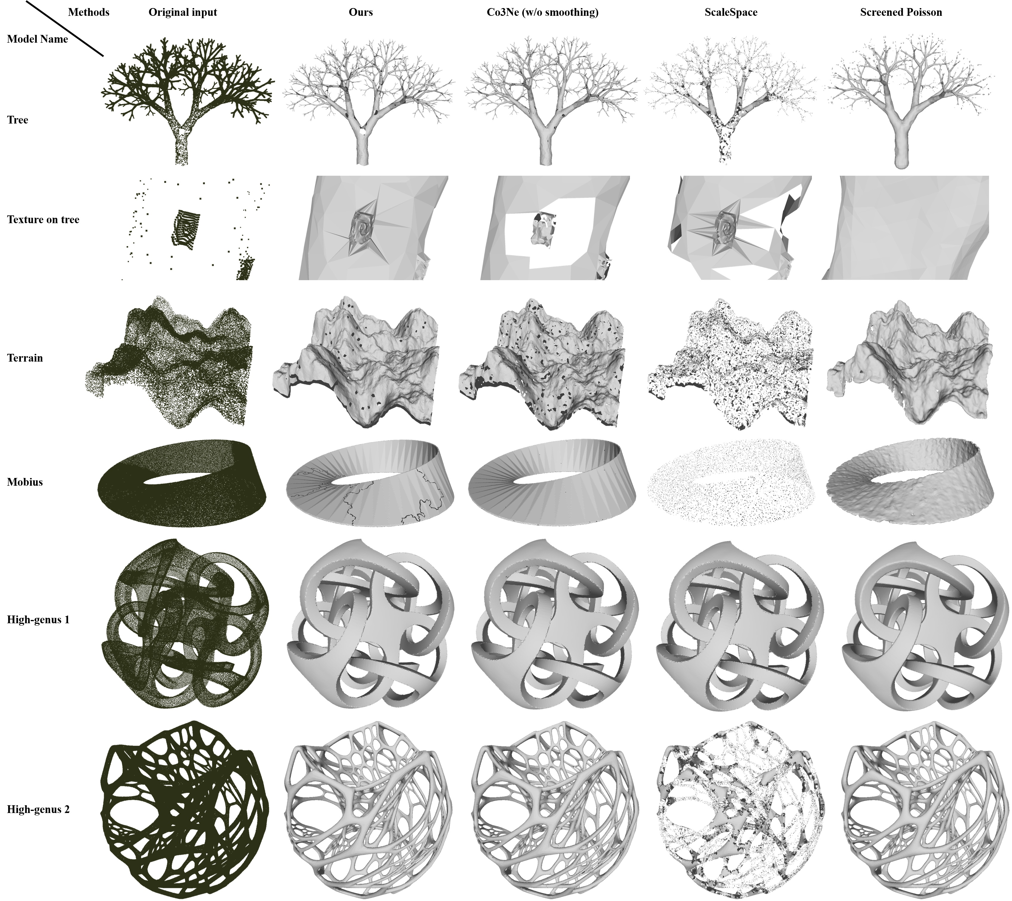
Figure 18. Visualization of the reconstruction results from four different methods on synthetic data.

5.3. Scanning datasets

In this section, we present the results of our method applied directly to optically acquired scans.

For these experiments, we use the projection distance as was discussed in Section 3.5. The experiments are performed on models from the three well-known public datasets: the Stanford 3D Scanning Repository, the DTU Robot Image Data Set (randomly downsampled to 500,000 points) (Jensen et al., 2014), and the S3DIS dataset(Armeni et al., 2016) with indoor scenes. The same comparisons are performed as for the tests on synthetic data.

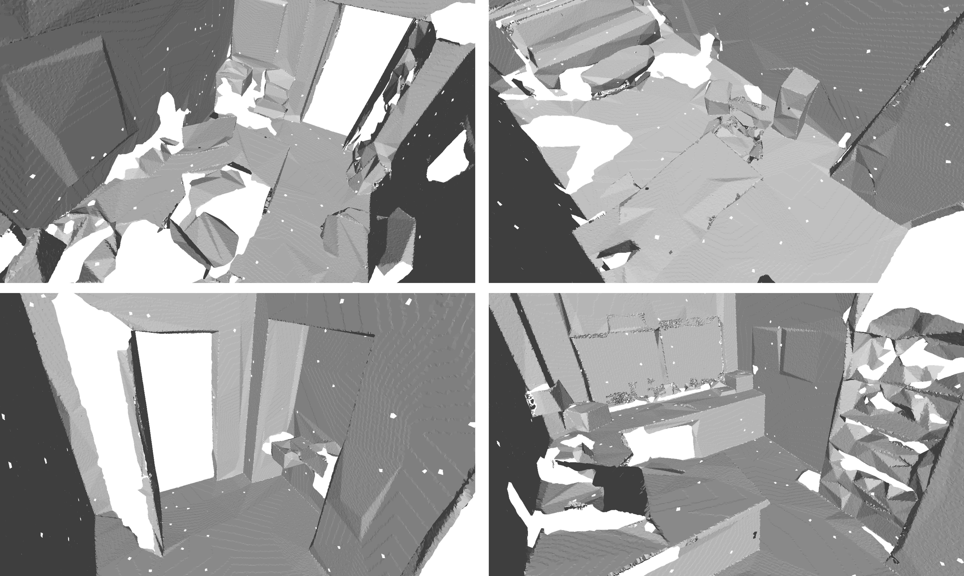
Figure 27. The reconstructed indoor scenes from four different rooms. Most of the area, e.g. walls, chairs, table are well reconstructed.

Figure 19 shows a comparison of our method against the three benchmark methods while Figure 27 shows the result on an acquired indoor scene. Table 4 contains the quantitative comparison. Figure 16 (bottom) shows three of the scanned models before and after denoising using bilateral normal filtering (Zheng et al., 2011).

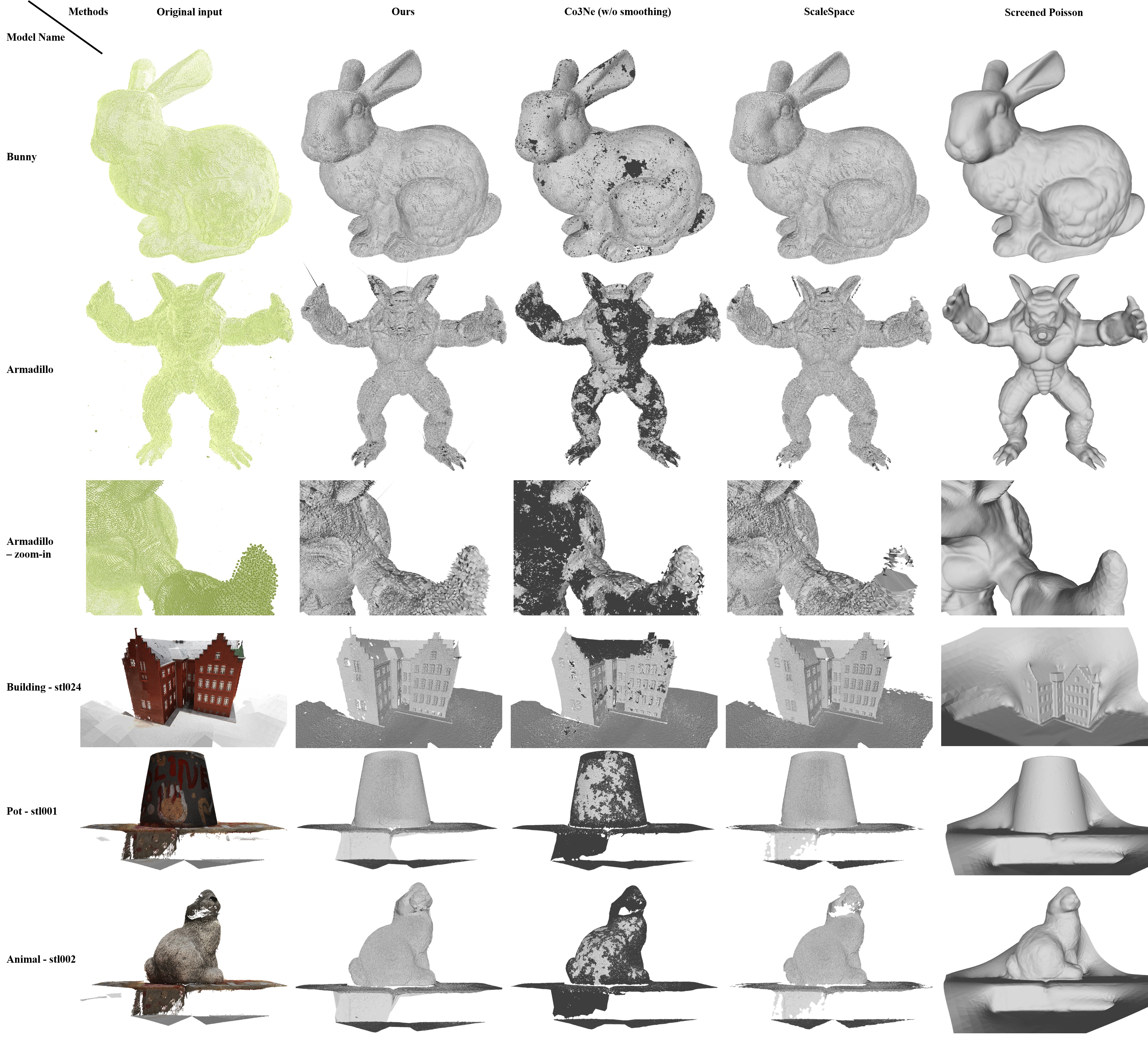
Figure 19. This is the visualization of the reconstruction results by four different methods. It can be noticed that ours, ScaleSpace, and Screened Poisson successfully reconstruct reasonable meshes of the input point cloud, while Co3Ne fails without the smoothing operation ahead. The black area on Co3Ne is mostly another layer of surface pointing in the opposite direction as it should be. Comparing ours and ScaleSpace, our method can reconstruct a more complete mesh with a smaller number of holes while ScaleSpace is restricted by the parameter of the Ball-Pivoting algorithm.

5.4. Parameter experiment

As discussed in Section 4.5, we conducted an experiment to provide a clearer insight into the parameter $k$ by varying its values. Figure 22 showcases the reconstructed results on the raw data of the Stanford Bunny with different values of $k$. Table 5 presents corresponding statistics for running time ($t(s)$) and peak memory usage ($m(GB)$). Unsurprisingly, resource utilization increases with $k$ while we see an increase in the number of holes for small $k$.

Table 5. Statistics for reconstruction with a range of $k$ value. Resource usage clearly increases with $k$ although the difference is slight for small $k$. However, for larger $k$ we see a significant increase in both memory consumption and time. This is largely due to the initialization where the larger graph is more costly.

$k$	5	10	15	30	60
$t(s)$	61	63	59	65	92
$m(GB)$	0.59	0.70	0.77	1.1	1.5

5.5. Explicit topology control

In this section, we conduct an experiment to emphasize a key strength of our method. The explicit control we have over the number of handles being connected allows us to control the output topology. A noteworthy and extensively studied shape is the cortical surface which always has genus 0. By specifying the anticipated genus within the program, our method can omit adding handles during the reconstruction process. In contrast, other methods consistently struggle to achieve this level of topology control, as illustrated in Figure 20. The experimented mesh is obtained from Brainder, created by Anderson Winkler.

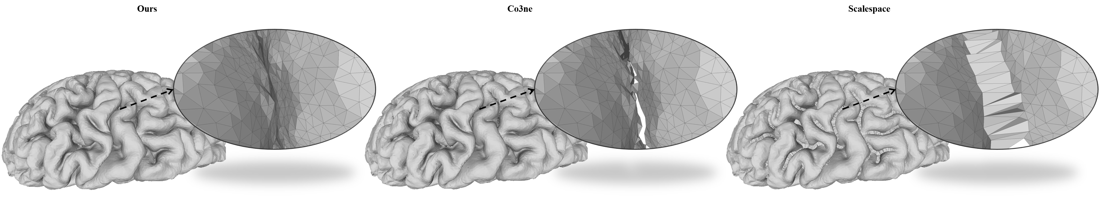
Figure 20. Reconstruction comparisons using a synthetic cortical surface point cloud. Our method successfully generated a genus-0 mesh, whereas Co3Ne retained only one side of the compressed opposite points, and Scalespace formed bridges across the gap.

5.6. Stress test

To investigate the robustness of our method against various common defects in input point clouds, a number of experiments were conducted. The common defects encompass noise in the point position, variations in normal direction, and misalignment.

5.6.1. Noise - point position

As we try to disentangle the influence of noise on point positions and normal directions, we compute the normal direction before the noise is added. To make the noise independent of scale, the noise vector is defined as:

(5) $$\mathbf{v_{n}}=A\cdot\overline{|e|}\cdot G(\mu,\sigma)\cdot\mathbf{v}\enspace,$$

where $\overline{|e|}$ is the average edge length of the reconstructed triangle mesh without noise. $A$ is the amplitude, $G(\mu,\sigma)$ gives a length following Gaussian distribution (where $\mu=0,\sigma=1$), and $\mathbf{v}$ gives a random direction in 3D space.

In addition to introducing random noise to the point positions, we further categorize the noise into two directions to assess its performance under stronger noise along both tangential and normal directions. The outcomes are depicted in Fig. 23. Remarkably, our method exhibits good robustness in the presence of noise affecting point positions.

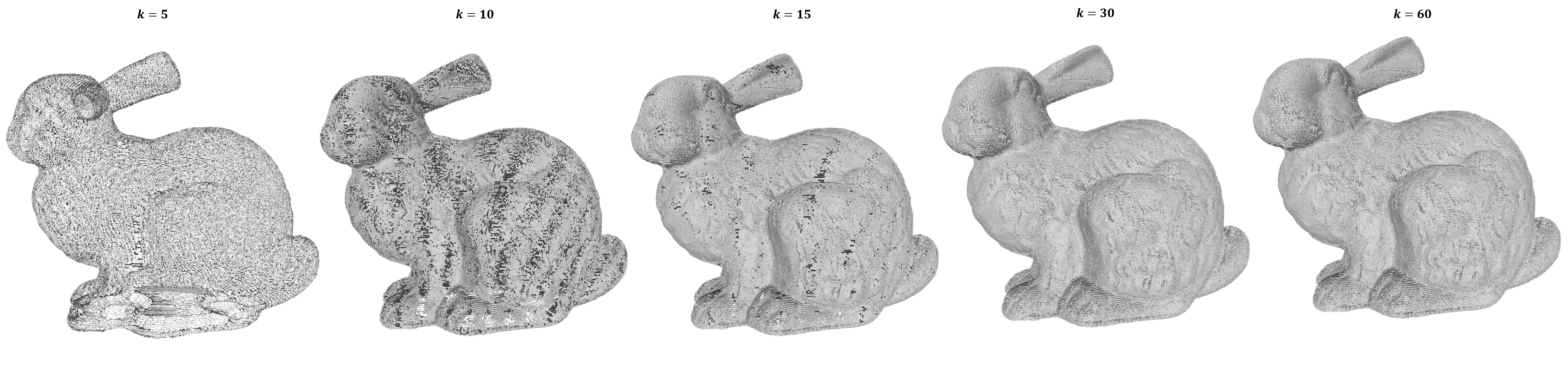
Figure 22. Qualitative result when increasing parameter $k$. The larger $k$ is, the more possible connections can be expected in the reconstructed result.

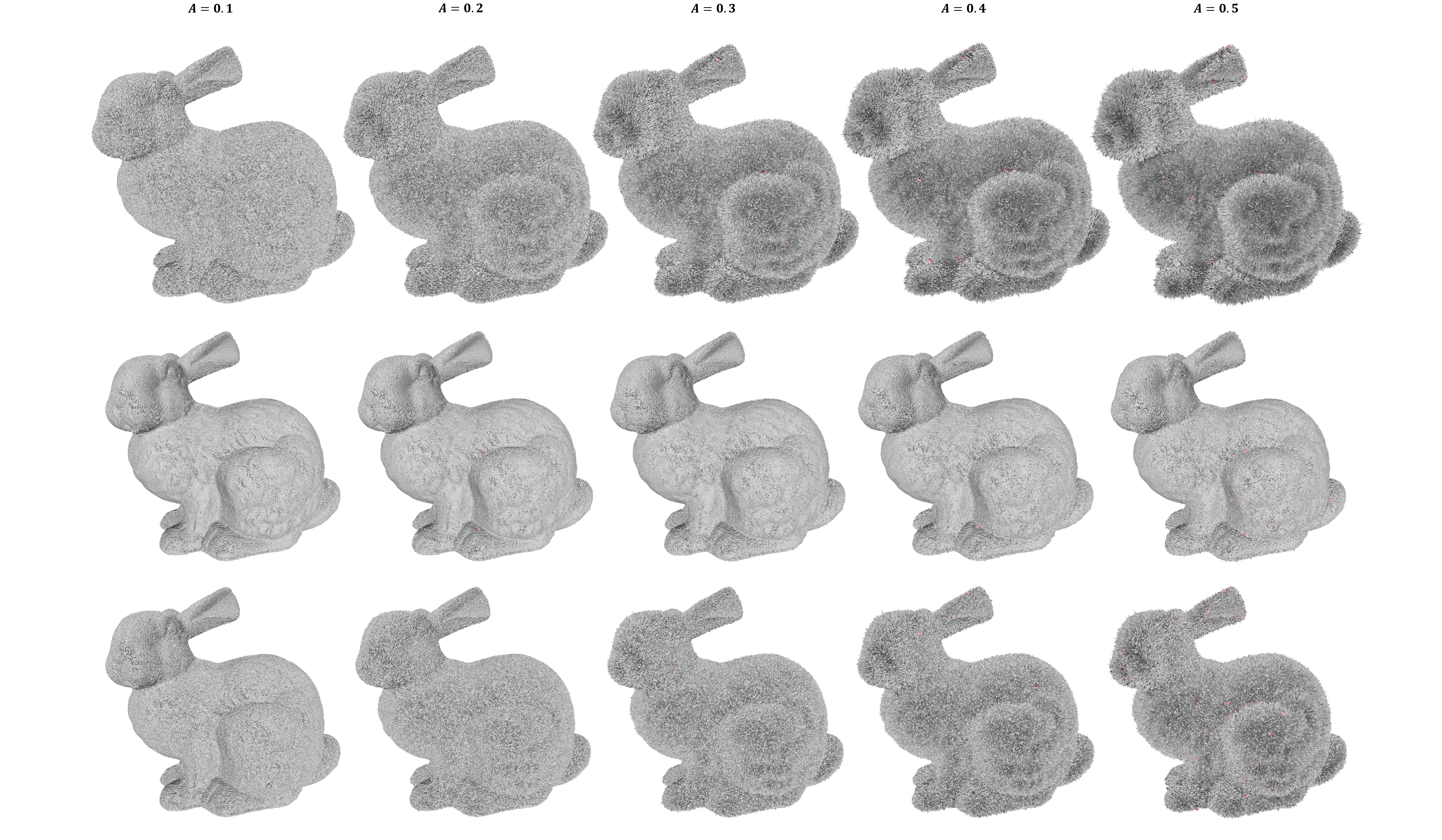
Figure 23. Noise experiment on the raw data of bunny. The first row shows the result of the experiment with noise following normal direction. The middle row depicts one in the tangential direction. While the last row is for fully random noise. The holes are rendered in red faces, it is hard to spot any holes with a glance.

5.6.2. Noise - normal direction

In this experiment, we introduce noise solely along the normal direction: this involves selecting a random direction and pivoting the normal by a constant angle $\theta$. The outcomes reveal that our method is sensitive to variations in the normal direction. When pivoting the normal away by an angle of 8 degrees, significant holes appear in the results.

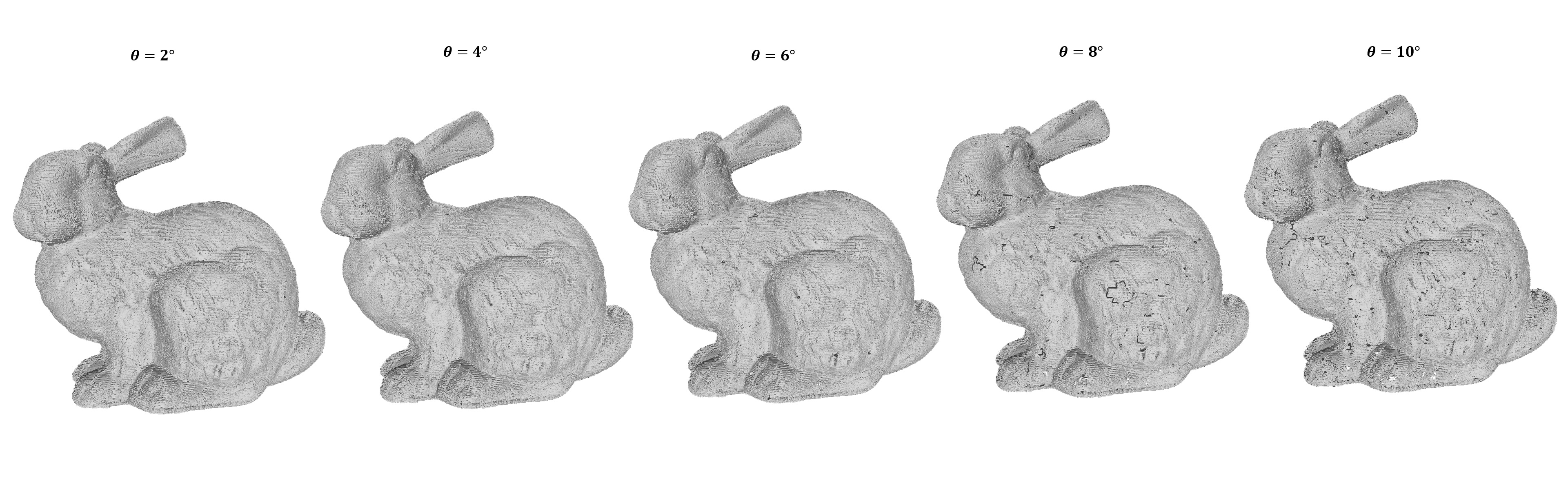
Figure 24. Noise experiment on normal direction.

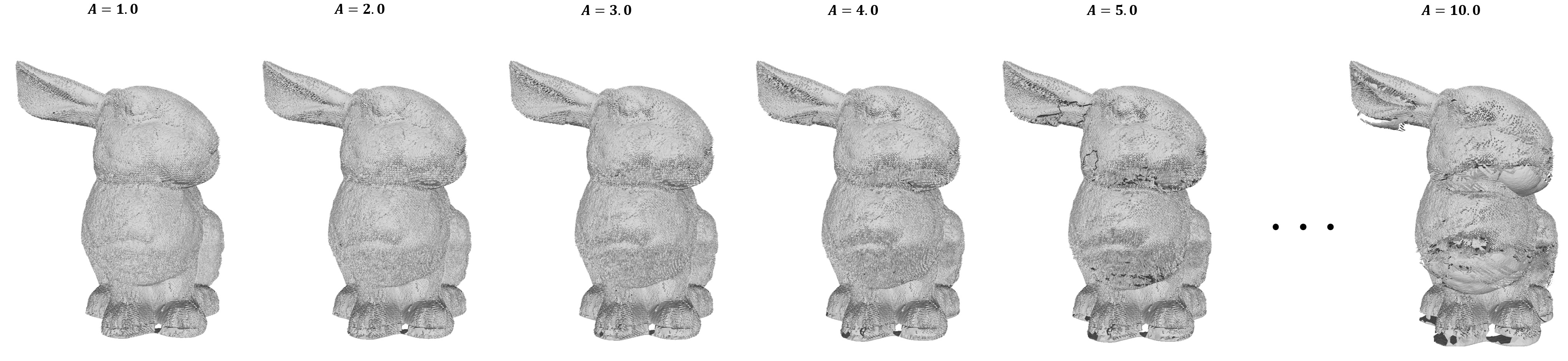
Figure 25. Misalignment experiment on the raw data of bunny.

5.6.3. Misalignment

Displacement

Another common defect in reconstruction is misalignment. To create artificial data, we take one point cloud file from the raw data of bunny (specifically, chin.ply) as the misaligned part. The point cloud is then gradually moved away from the registered position. The length of movement is defined as:

(6) $$d=A\cdot\overline{|e|}\cdot\mathbf{v}\enspace,$$

where $A$ is the changing amplitude, $\overline{|e|}$ is the average edge length, and $\mathbf{v}$ is the offset direction. Fig. 25 presents the results. Our method effectively addresses misalignment when it is minimal (less than 4 times the average length). However, as misalignment increases, normal estimation is impacted, leading to the emergence of holes. When the misalignment reaches a distance 10 times the average edge length away from the original position, it is deemed to represent another layer of surface, resulting in failure.

rotation & non-rigid misalignment

Besides displacement, other types of misalignment exist including rotational and non-rigid misalignment. Both types will create a situation where multiple layers of vertices with different normals coinhabit the same local region. If the normals are estimated from the combined point cloud, it is impossible to avoid connections between points from different layers. This leads to a situation where vertices from different layers connect with each other, often leading to holes in the reconstruction since the layers are prone to interpenetration which, of course, is a non-manifold configuration.

Examples are given through the failed reconstruction from the raw data of Stanford Happy Buddha in Fig. 26 (left). However, if the normal is accurately estimated before the alignment, no smoothing effect on normals will take place at the joint. Thus, our method will reconstruct both pieces correctly with the intersection at the joint, as the synthetic cross reconstruction shown in Fig. 26 (right). However, often the layers should be combined, and then we get a much more stable normal estimate if it is based on the combined point cloud. Hence, it is generally better to estimate the normals on the combined point cloud.

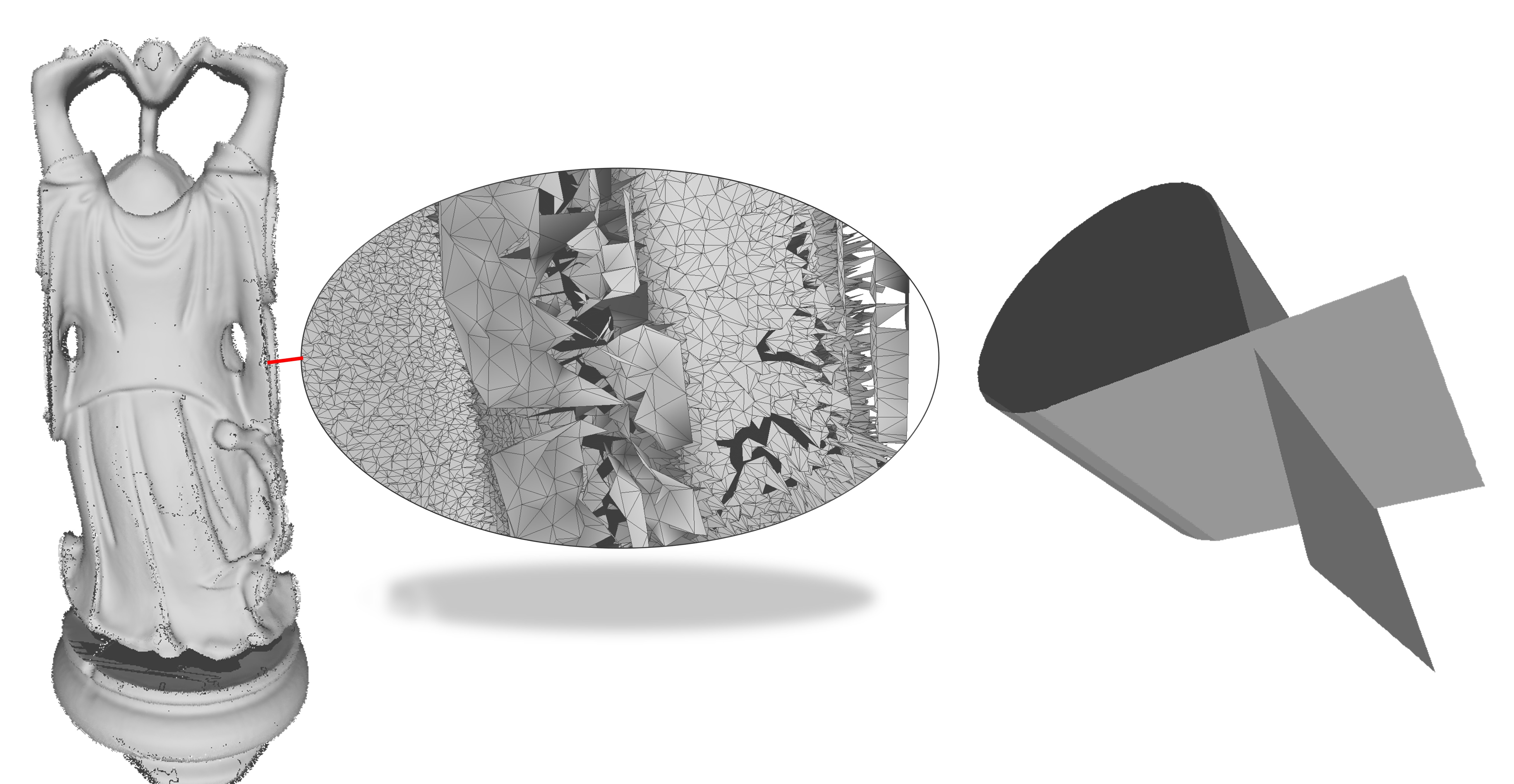
Figure 26. Left: reconstruction of the so-called Happy Buddha model from the original scan data is a fail case due to subscans which interpenetrate but still connect since points from all scans contribute to normal estimation. Right: synthetic case where a self-intersecting surface is resolved correctly by our approach by using exact normals to disambiguate.

6. Discussion

Our work is based on the simple observation that a tree connecting all points in a point cloud is a planar graph and, given a rotation system, we can construct a genus zero mesh with a single face that contains all points. The edges of that face are precisely the edges of the tree covered twice, and our results demonstrate that it is possible to triangulate this face by incrementally inserting edges. We can raise the genus by explicitly and judiciously adding handles.

The proposed method outputs a surface reconstruction where all inlier points that belong to the graph that we construct initially are also part of the output mesh. Many other methods reject points in order to construct the best possible output mesh, but in effect this means that reconstruction and noise reduction are subtly coupled. If this is desired it seems that volumetric methods might be more appropriate. In contrast, our method rejects no points and leaves it to the downstream processing to reduce noise. That can be beneficial for instance in applications where several sub-scans are combined, and it is desirable that there is no bias in how many point are kept from each sub-scan.

Compared to previous work, we initially make sure that connected vertices belong to the same face. This allows us to guarantee that gratuitous handles are not added. Of course, the true genus of the reconstructed object is not necessarily known. Hence, it is not generally possible to guarantee correct topology, but since we add handles explicitly, we can impose a a threshold on the handle quality.

The fact that handles are added explicitly also makes it trivial to restrict the topology of reconstructed objects that are known to be of sphere or disk topology since we can simply omit the insertion of handles. The utility of this was demonstrated in Section 5.5 where we used topology control to restrict the cortical surface reconstruction to genus 0. For objects of higher genus, we do need to insert handles, but we can still restrict the topology by only inserting handles (in prioritized order) till the desired genus is attained.

Like many other methods, we are reliant on consistently oriented normals. In principle, one could find a rotation system without normals, e.g. by searching for consistent circular orderings of edges at each vertex, but then the resulting rotation system would induce a consistent normal orientation. In return for our dependence on normals, we get the benefit of being able to utilize surface normals to disambiguate surfaces which are geometrically very close such as the two sides of the terrain in Section 5.2.2.

6.1. Limitations and Future Work

Our method is relatively robust to noise on the positions of the points, but susceptible to normal noise. Fortunately, the normal field only has to be smooth and not necessarily accurate with respect to the underlying surface, and in many practical scanning scenarios where points are noisy, we can obtain smooth normal estimates by using a large number of nearby points.

The main failure mode of our method is when point clouds consist of several scans that are so poorly aligned that they interpenetrate. In these cases, the underlying data is manifestly non-manifold, and, since we can only reconstruct manifold surfaces, this leads to faces that cannot be triangulated and, in turn, components of the mesh that disconnect from the rest of the model. In principle this could be remedied by only connecting points in the initial graph if either the points come from the same scan or their normals are very similar. This is something that we will consider more in future work.

A strong tool for furthering the practical performance of algorithms is that of parallelization. The current implementation is sequential, and while the algorithm isn’t embarrassingly parallel, we see ample opportunities to make use of parallelization.

The main hindrances to parallelization lie in initialization, and the splitting of faceloops. Luckily, libraries like the Boost Graph Library provides implementations for parallel computations of minimum spanning trees, leaving us to deal with parallel maintenance of faceloops. Recall that faceloops are represented as balanced binary trees, that once split, will never interact. Therefore it suffices to lock access to the single faceloop that is being processed, leaving the remaining trees open for manipulation in parallel. This will cause some congestion initially, but as the number of faces grows, so does the potential for parallelization.

- (1)
- Akleman and Chen (1999) Ergun Akleman and Jianer Chen. 1999. Guaranteeing the 2-Manifold Property for Meshes with Doubly Linked Face List. International Journal of Shape Modeling 05, 02 (1999), 159–177. https://doi.org/10.1142/S0218654399000150
- Akleman et al. (2003) Ergun Akleman, Jianer Chen, and Vinod Srinivasan. 2003. A minimal and complete set of operators for the development of robust manifold mesh modelers. Graphical Models 65, 5 (2003), 286–304. https://doi.org/10.1016/S1524-0703(03)00047-X Special Issue on SMI 2002.
- Amenta et al. (1998) Nina Amenta, Marshall Bern, and Manolis Kamvysselis. 1998. A new Voronoi-based surface reconstruction algorithm. In Proceedings of the 25th annual conference on Computer graphics and interactive techniques. 415–421.
- Amenta et al. (2000) Nina Amenta, Sunghee Choi, Tamal K Dey, and Naveen Leekha. 2000. A simple algorithm for homeomorphic surface reconstruction. In Proceedings of the sixteenth annual symposium on Computational geometry. 213–222.
- Amenta et al. (2001) Nina Amenta, Sunghee Choi, and Ravi Krishna Kolluri. 2001. The power crust. In Proceedings of the sixth ACM symposium on Solid modeling and applications. 249–266.
- Armeni et al. (2016) Iro Armeni, Ozan Sener, Amir R Zamir, Helen Jiang, Ioannis Brilakis, Martin Fischer, and Silvio Savarese. 2016. 3d semantic parsing of large-scale indoor spaces. In Proceedings of the IEEE conference on computer vision and pattern recognition. 1534–1543.
- Berger et al. (2017) Matthew Berger, Andrea Tagliasacchi, Lee M Seversky, Pierre Alliez, Gael Guennebaud, Joshua A Levine, Andrei Sharf, and Claudio T Silva. 2017. A survey of surface reconstruction from point clouds. 36, 1 (2017), 301–329.
- Bernardini et al. (1999) Fausto Bernardini, Joshua Mittleman, Holly Rushmeier, Cláudio Silva, and Gabriel Taubin. 1999. The ball-pivoting algorithm for surface reconstruction. IEEE transactions on visualization and computer graphics 5, 4 (1999), 349–359.
- Boissonnat (1984) Jean-Daniel Boissonnat. 1984. Geometric structures for three-dimensional shape representation. ACM Transactions on Graphics (TOG) 3, 4 (1984), 266–286.
- Boltcheva and Lévy (2017) Dobrina Boltcheva and Bruno Lévy. 2017. Surface reconstruction by computing restricted voronoi cells in parallel. Computer-Aided Design 90 (2017), 123–134.
- Cazals and Giesen (2004) Frédéric Cazals and Joachim Giesen. 2004. Delaunay Triangulation Based Surface Reconstruction: Ideas and Algorithms. Technical Report RR-5393. INRIA. 42 pages. https://inria.hal.science/inria-00070610
- Curless and Levoy (1996) Brian Curless and Marc Levoy. 1996. A volumetric method for building complex models from range images. In Proceedings of the 23rd annual conference on Computer graphics and interactive techniques. 303–312.
- Digne et al. (2011) Julie Digne, Jean-Michel Morel, Charyar-Mehdi Souzani, and Claire Lartigue. 2011. Scale space meshing of raw data point sets. 30, 6 (2011), 1630–1642.
- Edelsbrunner (2003) Herbert Edelsbrunner. 2003. Surface Reconstruction by Wrapping Finite Sets in Space. Springer Berlin Heidelberg, Berlin, Heidelberg, 379–404. https://doi.org/10.1007/978-3-642-55566-4_17
- Edmonds Jr (1960) John Robert Edmonds Jr. 1960. A Combinatorial Representation for Oriented Polyhedral Surfaces. Master of Arts. University of Maryland.
- Farshian et al. (2023) Anis Farshian, Markus Götz, Gabriele Cavallaro, Charlotte Debus, Matthias Nießner, Jón Atli Benediktsson, and Achim Streit. 2023. Deep-Learning-Based 3-D Surface Reconstruction—A Survey. Proc. IEEE 111, 11 (2023), 1464–1501. https://doi.org/10.1109/JPROC.2023.3321433
- Friedman et al. (1977) Jerome H. Friedman, Jon Louis Bentley, and Raphael Ari Finkel. 1977. An Algorithm for Finding Best Matches in Logarithmic Expected Time. ACM Trans. Math. Softw. 3, 3 (sep 1977), 209–226. https://doi.org/10.1145/355744.355745
- Henzinger and King (1999) Monika R. Henzinger and Valerie King. 1999. Randomized Fully Dynamic Graph Algorithms with Polylogarithmic Time per Operation. J. ACM 46, 4 (jul 1999), 502–516. https://doi.org/10.1145/320211.320215
- Hoppe et al. (1992) Hugues Hoppe, Tony DeRose, Tom Duchamp, John McDonald, and Werner Stuetzle. 1992. Surface reconstruction from unorganized points. In Proceedings of the 19th annual conference on computer graphics and interactive techniques. 71–78.
- Jensen et al. (2014) Rasmus Jensen, Anders Dahl, George Vogiatzis, Engin Tola, and Henrik Aanæs. 2014. Large scale multi-view stereopsis evaluation. In Proceedings of the IEEE conference on computer vision and pattern recognition. 406–413.
- Kazhdan et al. (2020) Misha Kazhdan, Ming Chuang, Szymon Rusinkiewicz, and Hugues Hoppe. 2020. Poisson surface reconstruction with envelope constraints. Computer Graphics Forum 39, 5 (2020), 173–182.
- Kazhdan and Hoppe (2013) Michael Kazhdan and Hugues Hoppe. 2013. Screened poisson surface reconstruction. ACM Transactions on Graphics (ToG) 32, 3 (2013), 1–13.
- Kazhdan et al. (2006) Michael M. Kazhdan, Matthew Bolitho, and Hugues Hoppe. 2006. Poisson Surface Reconstruction. In Proceedings of the Fourth Eurographics Symposium on Geometry Processing (Cagliari, Sardinia, Italy) (SGP ’06, Vol. 256), Alla Sheffer and Konrad Polthier (Eds.). Eurographics Association, Aire-la-Ville, Switzerland, Switzerland, 61–70.
- MacLane (1937) Saunders MacLane. 1937. A combinatorial condition for planar graphs. Fundamenta Mathematicae 28 (1937), 22–32.
- Mantyla and Sulonen (1982) Martti Mantyla and Reijo Sulonen. 1982. GWB: A solid modeler with Euler operators. IEEE Computer Graphics and Applications 2, 7 (1982), 17–31.
- Mencl (1995) Robert Mencl. 1995. A Graph-Based Approach to Surface Reconstruction. 14, 3 (1995), 445–456.
- Mencl and Müller (2004) Robert Mencl and Heinrich Müller. 2004. Empirical Analysis of Surface Interpolation by Spatial Environment Graphs. In Geometric Modeling for Scientific Visualization, Guido Brunnett, Bernd Hamann, Heinrich Müller, and Lars Linsen (Eds.). Springer Berlin Heidelberg, Berlin, Heidelberg, 51–65.
- Mencl and Müller (1998) Robert Mencl and Heinrich Müller. 1998. Graph-Based Surface Reconstruction Using Structures in Scattered Point Sets. In Proceedings - Computer Graphics International. 298–311. https://doi.org/10.1109/CGI.1998.694281
- Prusinkiewicz et al. (1996) Przemyslaw Prusinkiewicz, Mark Hammel, Jim Hanan, and Radomir Mech. 1996. L-systems: from the theory to visual models of plants. In Proceedings of the 2nd CSIRO Symposium on Computational Challenges in Life Sciences, Vol. 3. Citeseer, 1–32.
- Sharp and Ovsjanikov (2020) Nicholas Sharp and Maks Ovsjanikov. 2020. ”PointTriNet: Learned Triangulation of 3D Point Sets”. In Proceedings of the European Conference on Computer Vision (ECCV).
- Sulzer et al. (2021) R. Sulzer, L. Landrieu, R. Marlet, and B. Vallet. 2021. Scalable Surface Reconstruction with Delaunay-Graph Neural Networks. Computer Graphics Forum 40, 5 (2021), 157–167. https://doi.org/10.1111/cgf.14364 arXiv:https://onlinelibrary.wiley.com/doi/pdf/10.1111/cgf.14364
- Wang et al. (2022) Pengfei Wang, Zixiong Wang, Shiqing Xin, Xifeng Gao, Wenping Wang, and Changhe Tu. 2022. Restricted Delaunay Triangulation for Explicit Surface Reconstruction. ACM Transactions on Graphics 41, 5, Article 180 (oct 2022), 20 pages. https://doi.org/10.1145/3533768
- Zhao et al. (2023) Tong Zhao, Laurent Busé, David Cohen-Steiner, Tamy Boubekeur, Jean-Marc Thiery, and Pierre Alliez. 2023. Variational Shape Reconstruction via Quadric Error Metrics. In ACM SIGGRAPH 2023 Conference Proceedings (Los Angeles, CA, USA) (SIGGRAPH ’23). Association for Computing Machinery, New York, NY, USA, Article 45, 10 pages. https://doi.org/10.1145/3588432.3591529
- Zheng et al. (2011) Youyi Zheng, Hongbo Fu, Oscar Kin-Chung Au, and Chiew-Lan Tai. 2011. Bilateral Normal Filtering for Mesh Denoising. IEEE Transactions on Visualization and Computer Graphics 17, 10 (2011), 1521–1530. https://doi.org/10.1109/TVCG.2010.264
- Zhou and Jacobson (2016) Qingnan Zhou and Alec Jacobson. 2016. Thingi10K: A Dataset of 10,000 3D-Printing Models. arXiv preprint arXiv:1605.04797 (2016).