On $f$-Divergence Principled Domain Adaptation: An Improved Framework

Abstract

Unsupervised domain adaptation (UDA) plays a crucial role in addressing distribution shifts in machine learning. In this work, we improve the theoretical foundations of UDA proposed by Acuna et al. (2021) by refining their $f$-divergence-based discrepancy and additionally introducing a new measure, $f$-domain discrepancy ($f$-DD). By removing the absolute value function and incorporating a scaling parameter, $f$-DD yields novel target error and sample complexity bounds, allowing us to recover previous KL-based results and bridging the gap between algorithms and theory presented in Acuna et al. (2021). Leveraging a localization technique, we also develop a fast-rate generalization bound. Empirical results demonstrate the superior performance of $f$-DD-based domain learning algorithms over previous works in popular UDA benchmarks.

1 Introduction

Machine learning often faces the daunting challenge of domain shift, where the distribution of data in the testing environment differs from that used in training. Unsupervised Domain Adaptation (UDA) arises as a solution to this problem. In UDA, models are allowed to access to labelled source domain data and unlabelled target domain data, while the ultimate goal is to find a model that performs well on the target domain. The mainstream theoretical foundations of UDA, and more broadly, domain adaptation (Quionero-Candela et al., 2009), primarily rely on the seminal works of discrepancy-based theory (Ben-David et al., 2006, 2010). In particular, Ben-David et al. (2006, 2010) characterize the error gap between two domains using a hypothesis class-specified discrepancy measure e.g., $\mathcal{H}\Delta\mathcal{H}$-divergence. While these works initially focus on binary classification tasks and zero-one loss, Mansour et al. (2009a) extend the theory to a more general setting. Subsequently, this kind of theoretical framework was extended by various works (Cortes et al., 2015; Germain et al., 2013, 2016; Zhang et al., 2019, 2020; Acuna et al., 2021; Shui et al., 2022), all sharing some common properties such as the ability to estimate the proposed discrepancy from finite unlabeled samples. Importantly, these theoretical results often inspire the design of new algorithms, such as domain-adversarial training of neural networks (DANN) (Ganin et al., 2016) and Margin Disparity Discrepancy (MDD) (Zhang et al., 2019), directly motivated by $\mathcal{H}\Delta\mathcal{H}$-divergence.

Recently, Acuna et al. (2021) propose an $f$-divergence-based domain learning framework, which generalizes various previous frameworks (e.g., those based on $\mathcal{H}\Delta\mathcal{H}$-divergence and total variation) and have demonstrated great empirical successes. However, we argue that this framework has potential limitations, at least in three aspects.

First, their discrepancy measure is based on the variational representation of $f$-divergence in Nguyen et al. (2010) (cf. Lemma 2.1). Although this variational formula is commonly adopted, its weakness has been pointed out in several works (Ruderman et al., 2012; Jiao et al., 2017). For instance, from this formula, one cannot recover the well-known Donsker and Varadhan’s (DV) representation of KL divergence (Donsker & Varadhan, 1983). This reveals a second limitation: some existing domain adaptation or transfer learning theories are based on the DV representation of KL, such as (Wu et al., 2020; Bu et al., 2022; Wang & Mao, 2023a), and the framework by Acuna et al. (2021), although including KL as a special case of $f$-divergence, can not unify those theories. Furthermore and more critically, the discrepancy measure proposed by Acuna et al. (2021) contains an absolute value function, while the original variational representation does not. Notably, this absolute value function is necessary in their derivation of an target error upper bound, and the fundamental reason behind this is still due to the weak version of the variational representation relied upon. Specifically, a variational representation of an $f$-divergence is a lower bound of the divergence, but using a weak lower bound creates technical difficulties in proving an upper bound for target domain error. Acuna et al. (2021) chooses to add an absolute value function accordingly, potentially leading to an overestimation of the corresponding $f$-divergence. In fact, this absolute value function is removed in their proposed algorithm, termed $f$-Domain Adversarial Learning ($f$-DAL). While $f$-DAL outperforms both DANN and MDD in standard benchmarks, this choice exhibits a clear gap between their theory and algorithm.

In this work, to overcome these limitations and explore the full potential of $f$-divergence, we present an improved framework for $f$-divergence-based domain learning theory. Specifically, we employ a more advanced variational representation of $f$-divergence (cf. Lemma 2.2), independently developed by Agrawal & Horel (2020, 2021) and Birrell et al. (2022). After introducing some preliminaries, the organization of the remainder of the paper and our main contributions are summarized below.

• In Section 3, we revisit the theoretical analysis in Acuna et al. (2021), where we refine their $f$-divergence-based discrepancy by Lemma 2.2 while retaining the absolute value function in the definition. The resulting target error bound (cf. Lemma 3.1) and the KL-based generalization bound (cf. Theorem 3.1) complement the theoretical framework of Acuna et al. (2021).

• In Section 4, we design a novel $f$-divergence-based domain discrepancy measure, dubbed $f$-DD. Specifically, we eliminate the absolute value function from the definition used in Section 3, incorporating a scaling parameter instead. We then derive an upper bound for the target error (cf. Theorem 4.1) and the sample complexity bound for our $f$-DD. The generalization bound based on empirical $f$-DD naturally follows from these results. Notably, the obtained target error bound allows us to recover the previous KL-based result in Wang & Mao (2023a) (cf. Corollary 4.1).

• In Section 5, to improve the convergence rate of our $f$-DD based bound, we sharpen the bound using a localization technique (Bartlett et al., 2005; Zhang et al., 2020). The localized $f$-DD allows for a crisp application of the local Rademacher complexity based concentration results (Bartlett et al., 2005), while also enabling us to achieve a fast-rate target error bound (cf. Theorem 5.1). As a concrete example, we present a generalization bound based on localized KL-DD (cf. Theorem 5.2), where our proof techniques are directly connected to fast-rate PAC-Bayesian bounds (Catoni, 2007; Alquier, 2021) and fast-rate information-theoretic generalization bounds (Hellström & Durisi, 2021, 2022; Wang & Mao, 2023c).

• In Section 6, we conduct empirical studies based on our $f$-DD framework. We show $f$-DD outperforms the original $f$-DAL in three popular UDA benchmarks, with the best performance achieved by Jeffereys-DD. Additionally, we note that the training objective in $f$-DAL aligns more closely with our theory than with Acuna et al. (2021) (cf. Proposition 1). We also show that adding the absolute value function leads to overestimation and that optimizing the scaling parameter in $f$-DD may not be necessary in practical algorithms.

2 Preliminaries

Notations and UDA Setup

Throughout the paper, unless otherwise noted, we will use a capitalized letter to denote a random variable, and use the corresponding lower-case letter to denote its realization. Let $\mathcal{X}$ and $\mathcal{Y}$ be the input space and the label space. Let $\mathcal{H}$ be the hypothesis space, where each $h\in\mathcal{H}$ is a hypothesis mapping $\mathcal{X}$ to ${\cal Y}$.

Consider a single-source domain adaptation setting, where $\mu$ and $\nu$ are two unknown distributions on $\mathcal{X}\times\mathcal{Y}$, characterizing respectively the source domain and the target domain. Let $\mathcal{S}=\{\left(X_{i},Y_{i}\right)\}_{i=1}^{n}{\sim}\mu^{\otimes n}$ be a labeled source-domain sample and $\mathcal{T}=\{X_{j}\}_{j=1}^{m}{\sim}\nu^{\otimes m}$ be an unlabelled target-domain sample. We use $\hat{\mu}$ and $\hat{\nu}$ to denote the empirical distributions on ${\cal X}$ corresponding to $\mathcal{S}$ and $\mathcal{T}$, respectively. The objective of UDA is to find a hypothesis $h\in\mathcal{H}$ based on $\mathcal{S}$ and $\mathcal{T}$ that “works well” on the target domain.

Let $\ell:\mathcal{Y}\times\mathcal{Y}\to\mathbb{R}_{0}^{+}$ be a symmetric loss (i.e. $\ell(y,y)=0$ for all $y\in{\cal Y}$). The population risk for each $h\in\mathcal{H}$ in the target domain (i.e. target error) is defined as $R_{\nu}(h)\triangleq{{\mathbb{E}_{(X,Y)\sim\nu}}\left[\ell(h(X),Y)\right]},$ and the population risk in the source domain, $R_{\mu}(h)$, is defined in the same way. Since $\mu$ and $\nu$ are unknown to the learner, one often uses recourse to the empirical risk in the source domain, which, for a given $\mathcal{S}$, is defined as $R_{\hat{\mu}}(h)\triangleq{{\mathbb{E}_{(X,Y)\sim\hat{\mu}}}\left[\ell(h(X),Y)\right]}={\frac{1}{n}\sum_{i=1}^{n}\ell(h(X_{i}),Y_{i})}.$

With a little abuse of the notation, we will simply use $\ell(h,h^{\prime})$ to represent $\ell(h(x),h^{\prime}(x))$ when the same $x$ is evaluated. Additionally, following the conventional literature on domain adaptation theory (Mansour et al., 2009a), we assume that the loss function satisfies the triangle property. For the readers’ convenience, a summary of all the notations is provided in Table 5 in the Appendix.

Background on $f$-divergence

The family of $f$-divergence is defined as follows.

Definition 2.1.

Let $P$ and $Q$ be two distributions on $\Theta$. Let $\phi:\mathbb{R}_{+}\to\mathbb{R}$ be a convex function with $\phi(1)=0$. If $P\ll Q$, then $f$-divergence is defined as

$${\rm D}_{\phi}(P||Q)\triangleq{{\mathbb{E}_{Q}}\left[\phi\left(\frac{dP}{dQ}\right)\right]},$$

where $\frac{dP}{dQ}$ is a Radon-Nikodym derivative.

The $f$-divergence family contains many popular divergences. For instance, letting $\phi(x)=x\log{x}$ (or $x\log{x}+c(x-1)$ for any constant $c$) recovers the definition of KL divergence.

The $f$-divergence discrepancy measure by Acuna et al. (2021) is motivated by the variational formula of $f$-divergence that utilizes the Legendre transformation (LT).

Lemma 2.1 (Nguyen et al. (2010)).

Let $\phi^{*}$ be the convex conjugate of $\phi$, and $\mathcal{G}\!\!=\!\!\{g:\Theta\to{\rm dom}(\phi^{*})\}$. Then

$${\rm D}_{\phi}(P||Q)=\sup_{g\in\mathcal{G}}{{\mathbb{E}_{\theta\sim P}}\left[g(\theta)\right]}-{{\mathbb{E}_{\theta\sim Q}}\left[\phi^{*}(g(\theta))\right]},$$

However, it is well-known that the variational formula in Lemma 2.1 could not recover the the Donsker and Varadhan’s (DV) representation of KL divergence (cf. Lemma B.1). We will elaborate on this later.

Recently, Birrell et al. (2022) and Agrawal & Horel (2020, 2021) concurrently introduce a novel variational representation for $f$-divergence, which is also implicitly stated in Ben-Tal & Teboulle (2007, Theorem 4.2), as given below.

Lemma 2.2 (Agrawal & Horel (2020, Corollary 3.5)).

Any $f$-divergence can be written as

$${\rm D}_{\phi}(P||Q)\!\!=\!\sup_{g\in\mathcal{G}}{{\mathbb{E}_{\theta\sim P}}\left[g(\theta)\right]}-\!\inf_{\alpha\in\mathbb{R}}\!\left\{{{\mathbb{E}_{\theta\sim Q}}\left[\phi^{*}(g(\theta)\!+\!\alpha)\right]}\!-\!\alpha\right\}\!.$$

This variational representation is a “shift transformation” of Lemma 2.1 (i.e., $g\to g+\alpha$). Note that this representation shares the same optimal solution as Lemma 2.1 (clearly identified as the corresponding $f$-divergence), but Lemma 2.2 is considered tighter in the sense that the representation in Lemma 2.2 is flatter around the optimal solution. Birrell et al. (2022) provides a comprehensive study to justify this, and they also show that Lemma 2.2 can accelerate numerical estimation of $f$-divergences.

Here, to illustrate the advantage of Lemma 2.2, we use KL divergence as an example. Specifically, let $\phi(x)=x\log{x}-x+1$, then its conjugate function is $\phi^{*}(y)=e^{y}-1$. Substituting $\phi^{*}$ into Lemma 2.1, we have the LT-based KL:

$$\mathrm{D_{KL}}\left(P||Q\right)=\sup_{g\in\mathcal{G}}{{\mathbb{E}_{P}}\left[g(\theta)\right]}-{{\mathbb{E}_{Q}}\left[e^{g(\theta)}-1\right]}.$$ (1)

On the other hand, Lemma 2.2 will give us

$$\mathrm{D_{KL}}\left(P||Q\right)= \sup_{g\in\mathcal{G}}{{\mathbb{E}_{P}}\left[g(\theta)\right]}\!-\!\inf_{\alpha\in\mathbb{R}}\left\{{{\mathbb{E}_{Q}}\left[e^{g(\theta)+\alpha}\right]}\!-\!1\!-\!\alpha\right\}$$

$$= \sup_{g\in\mathcal{G}}{{\mathbb{E}_{P}}\left[g(\theta)\right]}-\log{{\mathbb{E}_{Q}}\left[e^{g(\theta)}\right]},$$ (2)

where the optimal $\alpha^{*}=-\log{{{{\mathbb{E}_{Q}}\left[e^{g(\theta)}\right]}}}$.

Notice that Eq. (2) immediately recovers the DV representation of KL. Since $\log(x)\leq x-1$ for $x>0$, it is evident that, as a lower bound of KL divergence, Eq. (2) is pointwise tighter than Eq. (1). In Appendix C, we also show the variational representations of some other divergences.

In the context of UDA, it may be tempting to think that using a point-wise smaller quantity (in Lemma 2.1), as the key component of an upper bound for target error, is essentially desired. However, neither Lemma 2.1 nor Lemma 2.2 is able to directly give such an upper bound. To elaborate, as $\phi^{*}(x)\geq x$ when $\phi(1)=0$ (cf. Lemma B.2), both Lemma 2.1 and Lemma 2.2 imply that $\mathrm{D}_{\phi}(P||Q)\leq\sup_{g}{{\mathbb{E}_{P}}\left[g(\theta)\right]}-{{\mathbb{E}_{Q}}\left[g(\theta)\right]}$. Bear this in mind, UDA typically requires an upper bound for the quantity $\sup_{h}{{\mathbb{E}_{\nu}}\left[\ell\circ h(X)\right]}-{{\mathbb{E}_{\mu}}\left[\ell\circ h(X)\right]}$, and simply restricting $\mathcal{G}$ in Lemma 2.1 and Lemma 2.2 to a composition of $\mathcal{H}$ and $\ell$ can only provide a lower bound for such a quantity.

Before we dedicate to an improved discrepancy measure, we first revisit the absolute discrepancy in Acuna et al. (2021) by using Lemma 2.2 instead. This also serves as a review of the common developments in the DA theory.

3 Warm-Up: Refined Absolute $f$-Divergence Domain Discrepancy

Based on Lemma 2.2, we refine the discrepancy measure of Acuna et al. (2021, Definition 3) as follows.

Definition 3.1.

For a given $h\in\mathcal{H}$, the $\widetilde{\rm D}^{h,\mathcal{H}}_{\phi}$ discrepancy is

$$\widetilde{\rm D}^{h,\mathcal{H}}_{\phi}(\mu||\nu)\triangleq\sup_{h^{\prime}\in\mathcal{H}}\left|{{\mathbb{E}_{\mu}}\left[\ell(h,h^{\prime})\right]}-I_{\phi,\nu}^{h}(\ell\circ h^{\prime})\right|,$$

where $I_{\phi,\nu}^{h}(\ell\circ h^{\prime})=\inf_{\alpha\in\mathbb{R}}\left\{{{\mathbb{E}_{\nu}}\left[\phi^{*}(\ell(h,h^{\prime})+\alpha)\right]}-\alpha\right\}$.

Remark 3.1.

Removing the absolute value function in $\widetilde{\rm D}^{h,\mathcal{H}}_{\phi}(\mu||\nu)$ does not alter its non-negativity. To see this, consider $h^{\prime}=h$. By the definitions of $\phi$ and $\phi^{*}$, $\inf_{\alpha}\phi^{*}(\alpha)-\alpha=\phi(1)=0$, we have ${{\mathbb{E}_{\nu}}\left[\ell(h,h^{\prime})\right]}=I_{\nu}^{\phi}(h,h^{\prime})=0$. Consequently, since $h$ exists in $\mathcal{H}$, $\widetilde{\rm D}^{h,\mathcal{H}}_{\phi}(\mu||\nu)\geq 0$ holds even without the absolute value function. In addition, due to the absolute value function, the relation between $\widetilde{\rm D}^{h,\mathcal{H}}_{\phi}(\mu||\nu)$ with the one in Acuna et al. (2021) is no longer clear.

While the absolute value function is not required for ensuring non-negativity, it is crucial for deriving the subsequent error bound for the target domain.

Lemma 3.1.

Let $\lambda^{*}=\min_{h^{*}\in\mathcal{H}}R_{\mu}(h^{*})+R_{\nu}(h^{*})$, then for any $h\in\mathcal{H}$, we have

$$R_{\nu}(h)\leq R_{\mu}(h)+\widetilde{\mathrm{D}}^{h,\mathcal{H}}_{\phi}(\mu||\nu)+\lambda^{*}.$$

This error bound shares similarities with the previous works (Ben-David et al., 2006, 2010; Zhang et al., 2019, 2020; Acuna et al., 2021). For example, the third term $\lambda^{*}$ is the ideal joint risk for the DA problem. As widely discussed in prior studies, this term captures the inherent challenge in the DA task and might be inevitable (Ben-David et al., 2010; Ben-David & Urner, 2012).

In the sequel, we will give a Rademacher complexity based generalization bound for the target error. Let $\hat{\mathfrak{R}}_{S}(\mathcal{F})$ denote the empirical Rademacher complexity of function class $\mathcal{F}=\{f:\mathcal{X}\to\mathbb{R}\}$ for some sample $S$ (Bartlett & Mendelson, 2002). Notice that a shift transformation of a function class will not change its Rademacher complexity, so the generalization bound based on $\widetilde{\mathrm{D}}^{h,\mathcal{H}}_{\phi}$ closely resembles the one presented in Acuna et al. (2021, Theorem 3), which contains a Lipschitz constant of $\phi^{*}$. Here, we give a generalization bound specialized for $\widetilde{\mathrm{D}}^{h,\mathcal{H}}_{\rm KL}$, wherein the Lipschitz constant of $\phi^{*}$ can be explicitly determined.

Theorem 3.1.

Let $\ell(\cdot,\cdot)\in[0,1]$. Then, for any $h\in\mathcal{H}$, with probability at least $1-\delta$, we have

$$R_{\nu}(h)\leq R_{\hat{\mu}} (h)+\widetilde{\mathrm{D}}^{h,\mathcal{H}}_{\rm KL}(\hat{\mu}||\hat{\nu})+2e\hat{\mathfrak{R}}_{\mathcal{S}}(\mathcal{H}^{\ell})+4\hat{\mathfrak{R}}_{\mathcal{T}}(\mathcal{H}^{\ell})$$

$$+{\lambda}^{*}+\mathcal{O}\left(\sqrt{\frac{\log(1/\delta)}{n}}+\sqrt{\frac{\log(1/\delta)}{m}}\right),$$

where $\mathcal{H}^{\ell}=\{x\mapsto\ell(h(x),h^{\prime}(x))|h,h^{\prime}\in\mathcal{H}\}$.

Acuna et al. (2021) also applies Rademacher complexity-based bound to further upper bound $\lambda^{*}$ by its empirical version, namely $\hat{\lambda}^{*}=\min_{h^{*}\in\mathcal{H}}R_{\hat{\mu}}(h^{*})+R_{\hat{\nu}}(h^{*})$. However, since there is no target label available, $R_{\hat{\nu}}(h^{*})$ is still uncomputable, invoking $\hat{\lambda}^{*}$ here has no clear advantage.

4 New $f$-Divergence-based DA Theory

While $\widetilde{\rm D}_{\phi}^{h,\mathcal{H}}$ serves as a valid domain discrepancy measure in DA theory, it exaggerates the domain difference without appropriate control. It’s noteworthy that Acuna et al. (2021) attempts to demonstrate their absolute discrepancy is upper bounded by ${\rm D}_{\phi}$ (Acuna et al., 2021, Lemma 1), but this is problematic; as $\sup{U}\geq 0$ does not imply $\sup{U}=\sup\left|U\right|$ when $U$ is not a positive function. When designing their $f$-DAL algorithm, they drop the absolute value function in their hypothesis-specified $f$-divergence (see Eq. (6)). Consequently, the remarkable performance of $f$-DAL reveals a significant gap from their theoretical foundation.

To bridge this gap, we introduce a new hypothesis-specific $f$-divergence-based DA framework. Our new discrepancy measure is dubbed $f$-domain discrepancy, or $f$-DD, defined without the absolute value function and with an affine transformation.

Definition 4.1 ($f$-DD).

For a given $h\in\mathcal{H}$, the $f$-DD measure ${\rm D}^{h,\mathcal{H}}_{\phi}$ is defined as

$${\rm D}^{h,\mathcal{H}}_{\phi}(\nu||\mu)\triangleq\sup_{h^{\prime}\in\mathcal{H},t\in\mathbb{R}}{{{\mathbb{E}_{\nu}}\left[t\cdot\ell(h,h^{\prime})\right]}-I_{\phi,\mu}^{h}(t\ell\circ h^{\prime})},$$

where $I_{\phi,\mu}^{h}(t\ell\circ h^{\prime})\!=\!\inf_{\alpha}\left\{{{\mathbb{E}_{\mu}}\left[\phi^{*}(t\cdot\ell(h,h^{\prime})+\alpha)\right]}\!-\!\alpha\right\}$.

Remark 4.1.

If $\mathcal{H}^{\ell}=\mathcal{G}$, ${\rm D}^{h,\mathcal{H}}_{\phi}(\nu||\mu)$ is an affine transformation of Lemma 2.1 (i.e. $g\to tg+\alpha$) and a scaling transformation of Lemma 2.2. Importantly, unlike $\widetilde{\rm D}_{\phi}^{h,\mathcal{H}}$, it’s easy to see that ${\rm D}^{h,\mathcal{H}}_{\phi}(\nu||\mu)\leq{\rm D}_{\phi}(\nu||\mu)$.

Our ${\rm D}^{h,\mathcal{H}}_{\phi}(\nu||\mu)$ retains some common properties of the discrepancies defined in the DA theory literature. First, as $t=0$ leads to ${{\mathbb{E}_{\nu}}\left[t\cdot\ell(h,h^{\prime})\right]}=I_{\phi,\mu}^{h}(t\ell\circ h^{\prime})=0$, the non-negativity of ${\rm D}^{h,\mathcal{H}}_{\phi}(\nu||\mu)$ is immediately justified. In addition, its asymmetric property is also preferred in DA, as discussed in the previous works (Zhang et al., 2019, 2020). Moreover, when $\mu=\nu$, by the definition of $\phi^{*}$, we have ${\rm D}^{h,\mathcal{H}}_{\phi}(\nu||\mu)=0$.

To present an error bound, the routine development, as in Lemma 3.1, is insufficient; we require a general version of the “change of measure” inequality, as given below.

Lemma 4.1.

Let $\psi(x)\triangleq\phi(x+1)$, and $\psi^{*}$ is its convex conjugate. Define $K_{h^{\prime},\mu}(t)\triangleq\inf_{\alpha}{{\mathbb{E}_{\mu}}\left[\psi^{*}(t\cdot\ell(h,h^{\prime})+\alpha)\right]}$. Let $K_{\mu}(t)=\sup_{h^{\prime}\in\mathcal{H}}K_{h^{\prime},\mu}(t)$, then for any $h,h^{\prime}\in\mathcal{H}$,

$$K^{*}_{\mu}\left({{\mathbb{E}_{\nu}}\left[\ell(h,h^{\prime})\right]}-{{\mathbb{E}_{\mu}}\left[\ell(h,h^{\prime})\right]}\right)\leq{\rm D}^{h,\mathcal{H}}_{\phi}(\nu||\mu),$$

where $K_{\mu}^{*}$ is the convex conjugate of $K_{\mu}$.

It is worth reminding that both $K_{\mu}$ and $K^{*}_{\mu}$ still depend on $h$, although we ignore $h$ in the notations to avoid cluttering. We are now ready to give a target error bound.

Theorem 4.1.

For any $h\in\mathcal{H}$, we have

$$R_{\nu}(h)\leq R_{\mu}(h)+\inf_{t\geq 0}\frac{\mathrm{D}^{h,\mathcal{H}}_{\phi}(\nu||\mu)+K_{\mu}(t)}{t}+\lambda^{*}.$$ (3)

Furthermore, let $\ell\in[0,1]$, if $\phi$ is twice differentiable and $\phi^{\prime\prime}$ is monotone, then

$$R_{\nu}(h)\leq R_{\mu}(h)+\sqrt{\frac{2}{\phi^{\prime\prime}(1)}{\mathrm{D}}^{h,\mathcal{H}}_{\phi}(\nu||\mu)}+\lambda^{*}.$$ (4)

As an application of Eq. (4), we consider the case of KL, namely ${\mathrm{D}}^{h,\mathcal{H}}_{\rm KL}(\nu||\mu)$. We have the following result.

Corollary 4.1.

Let $\ell\in[0,1]$, then for any $h\in\mathcal{H}$, we have

$$R_{\nu}(h)\leq R_{\mu}(h)+\sqrt{2{\mathrm{D}}^{h,\mathcal{H}}_{\rm KL}(\nu||\mu)}+\lambda^{*}.$$ (5)

As ${\mathrm{D}}^{h,\mathcal{H}}_{\rm KL}(\nu||\mu)\leq{\mathrm{D}}_{\rm KL}(\nu||\mu)$, the bound in Wang & Mao (2023a, Theorem 4.2) can be recovered by Corollary 4.1 for the same bounded loss function. We also remark that the boundedness assumption in Corollary 4.1 can be further relaxed by applying the same sub-Gaussian assumption as in Wang & Mao (2023a, Theorem 4.2).

To give a generalization bound, the next step involves obtaining a concentration result for $f$-DD, as given below.

Lemma 4.2.

Let $\ell\in[0,1]$ and let $t_{0}$ be the optimal $t$ achieving the superum in ${\rm D}^{h,\mathcal{H}}_{\phi}(\nu||\mu)$. Assume $\phi^{*}$ is $L$-Lipschitz, then for any given $h$, with probability at least $1-\delta$, we have

$${\rm D}^{h,\mathcal{H}}_{\phi}(\nu||\mu)\leq{\rm D}^{h,\mathcal{H}}_{\phi} (\hat{\nu}||\hat{\mu})\!+\!2\left|t_{0}\right|\hat{\mathfrak{R}}_{\mathcal{T}}(\mathcal{H}^{\ell})\!+\!2L\left|t_{0}\right|\hat{\mathfrak{R}}_{\mathcal{S}}(\mathcal{H}^{\ell})$$

$$+\mathcal{O}\left(\sqrt{\frac{\log(1/\delta)}{n}}+\sqrt{\frac{\log(1/\delta)}{m}}\right).$$

Remark 4.2.

The function $\phi^{*}$ needs not to be globally Lipschitz continues; it can be locally Lipschitz for a bounded domain. For example, in the case of KL, $\phi^{*}$ is $e$-Lipschitz continues when $\ell\in[0,1]$. Moreover, although $t_{0}$ might not always have a closed-form expression, in the case of $\chi^{2}$-DD, we know that $t_{0}=\frac{2\left({{\mathbb{E}_{\nu}}\left[\ell(h,h^{\prime*})\right]}-{{\mathbb{E}_{\mu}}\left[\ell(h,h^{\prime*})\right]}\right)}{\mathrm{Var}_{\mu}\left(\ell(h,h^{\prime*})\right)}$ where $h^{\prime*}$ is the corresponding optimal hypothesis.

It is also straightforward to obtain concentration results for $K_{\mu}(t)-K_{\hat{\mu}}(t)$ and $R_{\mu}(h)-R_{\hat{\mu}}(h)$. Substituting these results into Eq. (3) yields the final generalization bound based on $f$-DD. Or alternatively, one can directly substitute Lemma 4.2 into Eq. (4) (See Appendix D.6). However, in this case, the empirical $f$-DD and other terms in Lemma 4.2 will feature a square root, slowing down the convergence rate. We address this limitation in the following section.

5 Sharper Bounds via Localization

A localization technique in DA theory is recently studied in Zhang et al. (2020). We now incorporate it into our framework. First, we define a localized hypothesis space, formally referred to as the (true) Rashomon set (Breiman, 2001; Semenova et al., 2022; Fisher et al., 2019).

Definition 5.1 (Rashomon set).

Given a data distribution $\mu$, a hypothesis space $\mathcal{H}$ and a loss function $\ell$, for a Rashomon parameter $r\geq 0$, the Rashomon set $\mathcal{H}_{r}$ is an $r$-level subset of $\mathcal{H}$ defined as: $\mathcal{H}_{r}\triangleq\{h\in\mathcal{H}|R_{\mu}(h)\leq r\}$.

Notice that the Rashomon set $\mathcal{H}_{r}$ implicitly depends on the data distribution. In this paper, we specifically define $\mathcal{H}_{r}$ by the source domain distribution $\mu$. Then, we define our localized $f$-DD below.

Definition 5.2 (Localized $f$-DD).

For a given $h\in\mathcal{H}_{r_{1}}$, the localized $f$-DD from $\mu$ to $\nu$ is defined as

$${\rm D}^{h,\mathcal{H}_{r}}_{\phi}(\nu||\mu)\triangleq\sup_{h^{\prime}\in\mathcal{H}_{r},t\geq 0} {{\mathbb{E}_{\nu}}\left[t\ell(h,h^{\prime})\right]}-I^{h}_{\phi,\mu}(t\ell\circ h^{\prime}).$$

Remark 5.1.

Compared with $f$-DD, localized $f$-DD restricts $h$ to $\mathcal{H}_{r_{1}}$ and $h^{\prime}$ to $\mathcal{H}_{r}$, where $r_{1}$ and $r$ may or may not be equal. In addition, the scaling parameter $t$ is now restricted to $\mathbb{R}^{+}_{0}$ instead of $\mathbb{R}$.

Clearly, ${\rm D}^{h,\mathcal{H}_{r}}_{\phi}(\mu||\nu)$ is non-decreasing when $r$ increases, and it is upper bounded by ${\rm D}^{h,\mathcal{H}}_{\phi}(\mu||\nu)$.

As also mentioned at the end of the previous section, Eq. (4) of Theorem 4.1 (and Eq. (5) of Corollary 4.1), involves a square root function for $f$-DD, potentially indicative of a slow-rate bound (e.g., if $\mathrm{D}^{h,\mathcal{H}}_{\phi}\in\mathcal{O}(1/n)$, then the bound decays with $\mathcal{O}(1/\sqrt{n})$). We now show that how the localized $f$-DD achieves a fast-rate error bound.

Theorem 5.1.

For any $h\in\mathcal{H}_{r_{1}}$ and constants $C_{1},C_{2}\in(0,+\infty)$ satisfying $K_{h^{\prime},\mu}(C_{1})\leq C_{1}C_{2}{{\mathbb{E}_{\mu}}\left[\ell(h,h^{\prime})\right]}$ for any $h^{\prime}\in\mathcal{H}_{r}$, the following holds:

$$R_{\nu}(h)\leq R_{\mu}(h)+\frac{1}{C_{1}}{{\mathrm{D}}^{h,\mathcal{H}_{r}}_{\phi}(\nu||\mu)}+C_{2}R^{r}_{\mu}(h)+\lambda_{r}^{*},$$

where $\lambda_{r}^{*}=\min_{h^{*}\in\mathcal{H}_{r}}R_{\mu}(h^{*})+R_{\nu}(h^{*})$ and $R^{r}_{\mu}(h)=\sup_{h^{\prime}\in\mathcal{H}_{r}}{{\mathbb{E}_{\mu}}\left[\ell(h,h^{\prime})\right]}$.

Remark 5.2.

By the triangle property, $R^{r}_{\mu}(h)\leq r+r_{1}$. In this case, a small $r_{1}$ will reduce both the first term and the third term in the bound. However, determining the optimal value for $r$ is intricate. On the one hand, we hope $r$ is small so that ${\mathrm{D}}^{h,\mathcal{H}_{r}}_{\phi}(\nu||\mu)$ and $R^{r}_{\mu}(h)$ are both small. On the other hand, if $r$ is too small, specifically if $r<\lambda^{*}$, then it’s possible that $\lambda_{r}^{*}>\lambda^{*}$ because the optimal hypothesis minimizing the joint risk may not exist in $\mathcal{H}_{r}$. Additionally, if both $r_{1}$ and $r$ are too small, the effective space for optimizing $C_{1}$ and $C_{2}$ may also be limited. Therefore, the value of $r$ engenders a complex trade-off among the three terms.

Overall, we expect $r_{1}$ to be as small as possible, aligning with the principle of empirical risk minimization for the source domain in practice. We may let $r>\lambda^{*}$ so that the optimal hypothesis is guaranteed to exist in the Rashomon set $\mathcal{H}_{r}$. Furthermore, if $r+r_{1}$ is unavoidably large, we prefer a small $C_{2}$ so that $C_{2}R_{\mu}^{\prime}(h)$ is small. If $\lambda^{*}$ itself is negligible, we use a vanishing $r+r_{1}$. In this case, one can focus on minimizing $1/C_{1}$ while allowing $C_{2}$ to be large.

Combining Theorem 5.1 with Lemma 4.2 and following routine steps will obtain the generalization bound based on $f$-DD, where the local Rademacher complexity (Bartlett et al., 2005) will be involved. However, one may feel unsatisfied without an explicit clue for the condition $K_{h^{\prime},\mu}(C_{1})\leq C_{1}C_{2}{{\mathbb{E}_{\mu}}\left[\ell(h,h^{\prime})\right]}$ in Theorem  5.1. In fact, exploring concentration results under this condition is a central theme in obtaining fast-rate PAC-Bayesian generalization bounds (Catoni, 2007; Seldin et al., 2012; Tolstikhin & Seldin, 2013; Yang et al., 2019; Alquier, 2021) and the information-theoretic generalization bounds (Hellström & Durisi, 2021, 2022; Wang & Mao, 2023c, b). Building upon similar ideas from these works, we now establish a sharper generalization result for our localized KL-DD measure, where the fast-rate condition is more explicit.

One key ingredient is the following result.

Lemma 5.1.

Let $\ell\in[0,1]$, and let $C_{1}>0$ and $C_{2}\in(0,1)$ satisfy $\left(e^{C_{1}}-C_{1}-1\right)\left(1+C_{2}^{2}\min\{r_{1}+r,1\}\right)-tC_{2}\leq 0$. Then, for any $h\in\mathcal{H}_{r_{1}}$ and $h^{\prime}\in\mathcal{H}_{r}$, we have

$${{\mathbb{E}_{\nu}}\left[\ell(h,h^{\prime})\right]}\leq\inf_{C_{1},C_{2}}\frac{\mathrm{D}^{h,\mathcal{H}_{r}}_{\rm KL}({\nu}||{\mu})}{C_{1}}+(1+C_{2}){{\mathbb{E}_{\mu}}\left[\ell(h,h^{\prime})\right]}.$$

Remark 5.3.

As an extreme case, if $r+r_{1}\to 0$, then we let $C_{2}\to 1$, the condition in the lemma indicates that $C_{1}<1.26$. Hence, the optimal bound becomes ${{\mathbb{E}_{\nu}}\left[\ell(h,h^{\prime})\right]}\leq 0.79\mathrm{D}^{h,\mathcal{H}_{r}}_{\rm KL}({\nu}||{\mu})$. This bound remains valid even without $r+r_{1}\to 0$. It holds when the Rashomon set $H_{r}$ is “consistent” with a given $h$, meaning all hypotheses in $H_{r}$ have similar predictions to $h$ on the source domain data. As an another case, if $r+r_{1}\geq 1$ and $\sup_{h^{\prime}}{{\mathbb{E}_{\mu}}\left[\ell(h,h^{\prime})\right]}$ is also large, we may prefer a small $C_{2}$, such as setting $C_{2}=0.1$. This suggests $C_{1}<0.2$, resulting in the optimal bound ${{\mathbb{E}_{\nu}}\left[\ell(h,h^{\prime})\right]}-{{\mathbb{E}_{\mu}}\left[\ell(h,h^{\prime})\right]}\leq 5\mathrm{D}^{h,\mathcal{H}_{r}}_{\rm KL}({\nu}||{\mu})+0.1{{\mathbb{E}_{\mu}}\left[\ell(h,h^{\prime})\right]}$. The conditions in Lemma 5.1 are common in many fast-rate bound literature, such as Hellström & Durisi (2022, Theorem 3).

We are now in a position to give a fast-rate generalization bound for localized KL-DD.

Theorem 5.2.

Under the conditions in Lemma 5.1. For any $h\in\mathcal{H}_{r_{1}}$, with probability at least $1-\delta$, we have

$$R_{\nu} (h)\leq R_{\hat{\mu}}(h)\!+\!\frac{\mathrm{D}^{h,\mathcal{H}_{r}}_{\rm KL}(\hat{\nu}||\hat{\mu})}{C_{1}}\!+\!C_{2}R^{r}_{\mu}(h)\!+\!\mathcal{O}\left(\hat{\mathfrak{R}}_{\mathcal{T}}\left(\mathcal{H}^{\ell}_{r}\right)\right.$$

$$+\left.\hat{\mathfrak{R}}_{\mathcal{S}}\left(\mathcal{H}^{\ell}_{\max\{r,r_{1}\}}\right)\right)\!+\!\mathcal{O}\left(\frac{\log(1/\delta)}{n}\!+\!\frac{\log(1/\delta)}{m}\right)$$

$$+\mathcal{O}\left(\sqrt{\frac{(r_{1}+r)\log(1/\delta)}{n}}+\sqrt{\frac{r\log(1/\delta)}{m}}\right)+\lambda_{r}^{*}.$$

Remark 5.4.

Due to the non-negativity of $f$-DD, a similar generalization bound also applies to the Jeffereys divergence (or symmetrized KL divergence) (Jeffreys, 1946) counterpart, which is simply the sum of KL divergence and reverse KL divergence (i.e. $\mathrm{D}_{\rm KL}(\hat{\mu}||\hat{\nu})+\mathrm{D}_{\rm KL}(\hat{\nu}||\hat{\mu})$). Furthermore, considering the fact that $\mathrm{D}_{\rm KL}(\nu||\mu)\leq\log(1+\chi^{2}(\nu||\mu))\leq\chi^{2}(\nu||\mu)$ (Polyanskiy & Wu, 2023), one might anticipate a similar bound for $\chi^{2}$-DD, which we defer to Appendix D.10.

This generalization bound suggests that when $r+r_{1}$ is small, not only are the first four terms (including the local Rademacher complexities) reduced, but it also causes $\mathcal{O}\left(\frac{1}{n}+\frac{1}{m}\right)$ to dominate the convergence rate of the bound. In a practical algorithm, when empirical risk of source domain is always minimized to zero (i.e. the realizable case), then $r_{1}$ itself may have a fast vanishing rate (e.g., $\mathcal{O}(1/n)$).

Table 1: Accuracy (%) on the Office-31 benchmark.

Method	A $\rightarrow$ W	D $\rightarrow$ W	W $\rightarrow$ D	A $\rightarrow$ D	D $\rightarrow$ A	W $\rightarrow$ A	Avg
ResNet-50 (He et al., 2016)	68.4$\pm$0.2	96.7$\pm$0.1	99.3$\pm$0.1	68.9$\pm$0.2	62.5$\pm$0.3	60.7$\pm$0.3	76.1
DANN (Ganin et al., 2016)	82.0$\pm$0.4	96.9$\pm$0.2	99.1$\pm$0.1	79.7$\pm$0.4	68.2$\pm$0.4	67.4$\pm$0.5	82.2
MDD (Zhang et al., 2019)	94.5$\pm$0.3	98.4$\pm$0.1	100.0$\pm$.0	93.5$\pm$0.2	74.6$\pm$0.3	72.2$\pm$0.1	88.9
KL (Nguyen et al., 2022)	87.9$\pm$0.4	99.0$\pm$0.2	100.0$\pm$.0	85.6$\pm$0.6	70.1$\pm$1.1	69.3$\pm$0.7	85.3
$f$-DAL (Acuna et al., 2021)	95.4$\pm$0.7	98.8$\pm$0.1	100.0$\pm$.0	93.8$\pm$0.4	74.9$\pm$1.5	74.2$\pm$0.5	89.5
Ours (KL-DD)	94.9$\pm$0.7	98.7$\pm$0.1	100.0$\pm$.0	95.9$\pm$0.6	74.6$\pm$0.9	74.6$\pm$0.7	89.8
Ours (${\chi^{2}}$-DD)	95.3$\pm$0.2	98.7$\pm$0.1	100.0$\pm$.0	95.0$\pm$0.4	73.7$\pm$0.5	75.6$\pm$0.2	89.7
Ours (Jeffreys-DD)	94.9$\pm$0.7	99.1 $\pm$0.2	100.0$\pm$.0	95.9$\pm$0.6	76.0$\pm$0.5	74.6$\pm$0.7	90.1

Table 2: Accuracy (%) on the Office-Home benchmark.

Method	Ar$\to$Cl	Ar$\to$Pr	Ar$\to$Rw	Cl$\to$Ar	Cl$\to$Pr	Cl$\to$Rw	Pr$\to$Ar	Pr$\to$Cl	Pr$\to$Rw	Rw$\to$Ar	Rw$\to$Cl	Rw$\to$Pr	Avg
ResNet-50 (He et al., 2016)	34.9	50.0	58.0	37.4	41.9	46.2	38.5	31.2	60.4	53.9	41.2	59.9	46.1
DANN (Ganin et al., 2016)	45.6	59.3	70.1	47.0	58.5	60.9	46.1	43.7	68.5	63.2	51.8	76.8	57.6
MDD (Zhang et al., 2019)	54.9	73.7	77.8	60.0	71.4	71.8	61.2	53.6	78.1	72.5	60.2	82.3	68.1
$f$-DAL (Acuna et al., 2021)	54.7	71.7	77.8	61.0	72.6	72.2	60.8	53.4	80.0	73.3	60.6	83.8	68.5
Ours (KL-DD)	55.3	70.8	78.6	62.6	73.8	73.6	62.7	53.4	80.9	75.2	61.3	84.2	69.4
Ours ($\chi^{2}$-DD)	55.2	68.9	79.0	62.3	73.7	73.4	62.5	53.6	81.3	74.8	61.0	84.1	69.2
Ours (Jeffereys-DD)	55.5	74.9	79.5	64.3	73.8	73.9	63.9	54.7	81.3	75.2	61.6	84.2	70.2

Table 3: Accuracy (%) on the Digits datasets

Method	M$\to$U	U$\to$M	Avg
DANN (Ganin et al., 2016)	91.8	94.7	93.3
$f$-DAL (Acuna et al., 2021)	95.3	97.3	96.3
Ours (KL-DD)	95.7	98.1	96.9
Ours ($\chi^{2}$-DD)	95.4	97.3	96.4
Ours (Jeffereys-DD)	95.9	98.3	97.1

6 Algorithms and Experimental Results

6.1 Domain Adversarial Learning Algorithm

Adversarial Learning Obejective

In a practical algorithm, the hypothesis space consists of two components: the representation part, denoted as $\mathcal{H}_{\rm rep}=\{h_{\rm rep}:\mathcal{X}\to\mathcal{Z}\}$, where $\mathcal{Z}$ is the representation space (e.g., the hidden output of a neural network), and the classification part, denoted as $\mathcal{H}_{\rm cls}=\{h_{\rm cls}:\mathcal{Z}\to\mathcal{Y}\}$. Therefore, the entire hypothesis space is given by $\mathcal{H}=\{h_{\rm cls}\circ h_{\rm rep}|h_{\rm rep}\in\mathcal{H}_{\rm rep},h_{\rm cls}\in\mathcal{H}_{\rm cls}\}$. The training objective in $f$-DAL (Acuna et al., 2021) is then formulated as:

$$\min_{h\in\mathcal{H}}\max_{h^{\prime}\in\mathcal{H^{\prime}}}R_{\hat{\mu}}(h)+\eta\tilde{d}_{\hat{\mu},\hat{\nu}}(h,h^{\prime}).$$ (6)

Here, $\tilde{d}_{\hat{\mu},\hat{\nu}}(h,h^{\prime})={{\mathbb{E}_{\hat{\nu}}}\left[\hat{\ell}(h,h^{\prime})\right]}-{{\mathbb{E}_{\hat{\mu}}}\left[\phi^{*}\left(\hat{\ell}(h,h^{\prime})\right)\right]}$, where $\eta$ is a trade-off parameter and $\hat{\ell}$ is the surrogate loss used to evaluate the disagreement between $h$ and $h^{\prime}$, which may or may not be the same as $\ell$. Note that, to better align with our framework, we change the order of $\hat{\mu}$ and $\hat{\nu}$ in $\tilde{d}_{\hat{\mu},\hat{\nu}}$ in the original $f$-DAL. This modification is minor, as in either case, its optimal value belongs to $f$-divergence (such as KL and reverse KL, $\chi^{2}$ and reverse $\chi^{2}$).

Eq. (6) results in an adversarial training strategy. Specifically, the outer optimization spans the entire hypothesis space. Meanwhile, within the inner optimization, given a $h=h_{\rm rep}\circ h_{\rm cls}$, the representation component $h_{\rm rep}$ is shared for $h^{\prime}$. In other words, the optimization is carried out for $h^{\prime}$ in $\mathcal{H}^{\prime}=\mathcal{H}_{\rm cls}\circ h_{\rm rep}\triangleq\{h_{\rm cls}\circ h_{\rm rep}|h_{\rm cls}\in\mathcal{H}_{\rm cls}\}$.

Clearly, as also discussed previously, $\max_{h^{\prime}}\tilde{d}_{\hat{\mu},\hat{\nu}}(h,h^{\prime})\leq\max_{h^{\prime}}\left|\tilde{d}_{\hat{\mu},\hat{\nu}}(h,h^{\prime})\right|$, which presents a clear gap between the theory and algorithms in Acuna et al. (2021). In contrast, this training objective aligns more closely with our $\mathrm{D}_{\phi}^{h,\mathcal{H}}$. Formally, we have the following result.

Proposition 1.

Let $d_{\hat{\mu},\hat{\nu}}(h,h^{\prime})={{\mathbb{E}_{\hat{\nu}}}\left[\hat{\ell}(h,h^{\prime})\right]}-I_{\phi,\hat{\mu}}^{h}(\hat{\ell}\circ h^{\prime})$. Assume $\hat{\ell}:\mathcal{X}\to\mathbb{R}$, we have $\max_{h^{\prime}}\tilde{d}_{\hat{\mu},\hat{\nu}}(h,h^{\prime})=\max_{h^{\prime}}d_{\hat{\mu},\hat{\nu}}(h,h^{\prime})=\mathrm{D}_{\phi}^{h,\mathcal{H}^{\prime}}(\hat{\nu}||\hat{\mu})\leq\mathrm{D}_{\phi}(\hat{\nu}||\hat{\mu})$.

In our algorithm, we use $d_{\hat{\mu},\hat{\nu}}(h,h^{\prime})$ to replace $\tilde{d}_{\hat{\mu},\hat{\nu}}(h,h^{\prime})$ in Eq. (6). Proposition 1 implies that either the optimal $\tilde{d}_{\hat{\mu},\hat{\nu}}(h,h^{\prime})$ or the optimal $d_{\hat{\mu},\hat{\nu}}(h,h^{\prime})$ coincides with $f$-DD. Moreover, as $\hat{\ell}$ is typically unbounded in practice (e.g., cross-entropy loss), considering the unbounded nature of $t$, Proposition 1 suggests an equivalence between optimizing $\hat{\ell}(h,h^{\prime})$ through $h^{\prime}$ and optimizing $t\ell(h,h^{\prime})$ through both $t$ and $h^{\prime}$. In this sense, $f$-DAL has already considered the scaling transformation. Later on we will empirically investigate whether explicitly optimizing $t$ is necessary.

Discrepancy Measures

In our algorithms, we mainly focus on three specific discrepancy measures: KL-DD, $\chi^{2}$-DD and the weighted Jeffereys-DD. Specifically, the weighted Jeffereys-DD is $\gamma_{1}\mathrm{D}_{\rm KL}(\hat{\mu}||\hat{\nu})+\gamma_{2}\mathrm{D}_{\rm KL}(\hat{\nu}||\hat{\mu})$, where $\gamma_{1}$ and $\gamma_{2}$ are tunable hyper-parameters. We note that Jeffereys divergence is not explored in Acuna et al. (2021) while it is also an $f$-divergence with $\phi(x)=(x-1)\log{x}$, and advantages of Jeffereys divergence are studied in (Bu et al., 2022; Nguyen et al., 2022; Wang & Mao, 2023a).

6.2 Experiments

The goals of our experiments unfold in three aspects: 1) demonstrating that utilizing the $f$-DD measure (i.e., using $d_{\hat{\mu},\hat{\nu}}(h,h^{\prime})$ as the training objective) leads to superior performance on the benchmarks; 2) confirming that the absolute discrepancy (i.e. $\left|\tilde{d}_{\hat{\mu},\hat{\nu}}(h,h^{\prime})\right|$) leads to a degradation in performance; 3) showing that optimizing over $t$ may be unnecessary in practical scenarios.

Dataset

We use three benchmark datasets: 1) the Office31 dataset (Saenko et al., 2010), which comprises $4,652$ images across $31$ categories. This dataset includes three domains: Amazon (A), Webcam (W) and DSLR (D); 2) the Office-Home dataset (Venkateswara et al., 2017), consisting of $15,500$ images distributed among four domains: Artistic images (Ar), Clip Art (Cl), Product images (Pr), and Real-world images (Rw); and 3) two Digits datasets, MNIST and USPS (Hull, 1994) with the associated domain adaptation tasks MNIST $\to$ USPS (M$\to$U) and USPS $\to$ MNIST (U$\to$M). We follow the splits and evaluation protocol established by Long et al. (2018), where MNIST and USPS have $60,000$ and $7,291$ training images, as well as $10,000$ and $2,007$ test images, respectively.

Table 4: Comparison between KL-DD and OptKL-DD

Method	Office-31	Office-Home	Digits
KL-DD	89.8	69.4	96.9
OptKL-DD	89.6	69.2	96.5

Baselines and Implementation Details

The primary baseline for our study is the preceding $f$-DAL (Acuna et al., 2021). Note that, with the exception of Digits, the results reported by Acuna et al. (2021) for $f$-DAL rely on maximum values obtained from their $\chi^{2}$-divergence and weighted Jensen-Shannon divergence across individual sub-tasks. In our comparison, we also include DANN (Ganin et al., 2016) and MDD (Zhang et al., 2019) as they may be interpreted as special cases of $f$-DAL. Furthermore, we compare the results reported by Nguyen et al. (2022) on the Office-31 dataset, although denoted as “KL”, their method incorporates Jeffereys divergence in their algorithms.

Our implementation closely follows Acuna et al. (2021). For Office-31 and Office-Home, we utilize a pretrained ResNet-50 (He et al., 2016) as the backbone network, while both the primary classifier in $h$ and the auxiliary classifier in $h^{\prime}$ consist of two-layer Leaky-ReLU networks. In the case of Digits, we employ LeNet (LeCun et al., 1998) as the backbone network and a two-layer ReLU network with Dropout ($0.5$) for the classifiers. Other hyper-parameter settings and the evaluation protocol remain consistent with Acuna et al. (2021), and the reported results represent average accuracies over $3$ different random seeds.

Boosted Benchmark Performance by $f$-DD

Tables 1-3 collectively demonstrate the superior performance of our weighted Jeffereys-DD compared to other methods across the three benchmarks. Notably, the most significant improvement over $f$-DAL is observed on Office-Home ($70.2\%$ vs $68.5\%$). Remarkably, this performance even surpasses the combination of $f$-DAL with a sampling-based implicit alignment approach (Jiang et al., 2020) (See Table 6 in Appendix), specifically designed to handle the label shift issues. In addition, unlike findings in Acuna et al. (2021), where $\chi^{2}$ outperforms other methods on nearly all tasks, our use of a tighter variational representation-based discrepancy reveals that $\chi^{2}$ is no longer superior to KL. In fact, our KL-DD slightly outperforms $\chi^{2}$-DD across all three benchmarks.

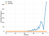
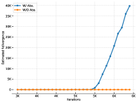
Figure 1: Failure of absolute discrepancy. The $y$-axis is the estimated $f$-divergence.

Failure of Absolute Discrepancy

We also perform experiments on A$\to$D and Ar$\to$Cl using the absolute discrepancy (i.e., $\max\left|\tilde{d}_{\hat{\mu},\hat{\nu}}(h,h^{\prime})\right|$). Specifically, we compare the $\chi^{2}$-based discrepancy with (w/) and without (w/o) the absolute value function. Figure 1 illustrates that such a discrepancy can easily explode during training, demonstrating its tendency to overestimate $f$-divergence. Additional results for KL is given in Figure 2 in Appendix.

Optimizing over $t$

In the paragraph following Proposition 1, we discuss the observation that optimizing over $t$ may not be necessary. Empirical evidence indicates that setting $t=1$ with hyper-parameter tuning (e.g., through $\eta$) yields satisfactory performance. Now, let’s delve into the selection of $t$ for KL-DD. Instead of using a stochastic gradient-based optimizer for updating $t$, we opt for a quadratic approximation for the optimal $t$, as studied in Birrell et al. (2022). Specifically, we define a Gibbs measure $d\mu^{\prime}=\frac{e^{{\ell}(h,h^{\prime})}d\mu}{{{\mathbb{E}_{\mu}}\left[e^{{\ell}(h,h^{\prime})}\right]}}$, then the optimal $t^{*}\approx 1+\Delta t^{*}$, where $\Delta t^{*}=\frac{{{\mathbb{E}_{\nu}}\left[{\ell}(h,h^{\prime})\right]}-{{\mathbb{E}_{\mu^{\prime}}}\left[\ell(h,h^{\prime})\right]}}{\mathrm{Var}_{\mu^{\prime}}(\ell(h,h^{\prime}))}$. Interested readers can find a detailed derivation of this approximation in Birrell et al. (2022, Appendix B). Substituting $t=1+\Delta t^{*}$, we have the training objective for the approximately optimal KL-DD (OptKL-DD). Table 4 presents an empirical comparison between OptKL-DD and the original KL-DD, where $t$ is simply set to 1. The results indicate that OptKL-DD does not offer any improvement on these benchmarks. Similar observations also hold for $\chi^{2}$, in which case optimal $t$ has an analytic form (see Appendix E), suggesting that using $t=1$, at least for KL and $\chi^{2}$, might be sufficient in practice.

Additional empirical results, including an ablation study on $\eta$ and t-SNE (Van der Maaten & Hinton, 2008) visualizations, can be found in Appendix E.

7 Other Related Works

Domain Adaptation

Apart from those mentioned in the introduction, various other discrepancy measures are explored in DA theories and algorithms. These include the Wasserstein distance (Flamary et al., 2016; Courty et al., 2017; Shen et al., 2018), Maximum Mean Discrepancy (Huang et al., 2006; Gong et al., 2013), second-order statistics alignment (Sun & Saenko, 2016; Sun et al., 2016), transfer exponents (Hanneke & Kpotufe, 2019; Hanneke et al., 2023), Integral Probability Metrics (Dhouib & Maghsudi, 2022) and so on. Additionally, one of our baseline models Nguyen et al. (2022) diverges from the adversarial training strategy. Instead, they minimize the KL divergence between two isotropic Gaussian distributions (source domain Gaussian and target domain Gaussian) in the representation space. Here, the Gaussian means and variances correspond to the hidden outputs of the representation network. The comparison between their KL-guided framework and our KL-DD is akin to the distinction between VAEs (Kingma & Welling, 2013) and GANs (Goodfellow et al., 2014). For further literature on DA theory, readers are directed to a recent survey by Redko et al. (2020).

$f$-divergence

The combination of $f$-divergence and adversarial training schemes has been extensively studied in generative models, including $f$-GAN (Nowozin et al., 2016; Song & Ermon, 2020), $\chi^{2}$-GAN (Tao et al., 2018) and others. In the DA context, Wu et al. (2019) introduce a $f$-divergence-based discrepancy measure while still relying on Lemma 2.1 and focusing solely on the Jensen-Shannon case. Additionally, Mansour et al. (2009b) investigates $\alpha$-Rényi divergence for multi-source DA, and Bruns-Smith et al. (2022) provides some intriguing interpretations of $\chi^{2}$-divergence-based generalization bound for covariate shifts.

8 Conclusion and Future Work

We have presented an improved approach for integrating $f$-divergence into DA theory. Theoretical contributions include novel DA generalization bounds, including fast-rate bounds via localization. On the practical front, the revised $f$-divergence-based discrepancy improves benchmark performance. Several promising future directions emerge from our work. Firstly, beyond its usefulness for local Rademacher complexity, the Rashomon set $\mathcal{H}_{r}$ also relates to another generalization measure, Rashomon ratio (Semenova et al., 2022), which may give an alternative perspective on generalization in DA. Additionally, exploring transfer component-based analysis (Hanneke & Kpotufe, 2019) for tight minimax rates in DA, leveraging a power transformation instead of the affine transformation in $f$-DD, holds promise.

The structure of the Appendix is outlined as follows: Section A provides a table summarizing the notations used throughout the paper. In Section B, we present a collection of technical lemmas crucial to our analysis. Additional variational representations for certain $f$-divergences are explored in Section C. Section D restates our theoretical results, provides detailed proofs, and introduces supplementary theoretical findings. For more details about experiments and additional empirical results, refer to Section E.

Appendix A Summary of Notations

For easy reference, Table 5 summarizes the key notations used in this paper.

Table 5: Summary of notations.

Notation	Definition
$\mathcal{X}$, $\mathcal{Y}$, $\mathcal{H}$	input, label and hypothesis space
$\mu$, $\nu$	source domain distribution and target domain distribution
$\mathcal{S}$, $\mathcal{T}$	source sample $\mathcal{S}=\{(X_{i},Y_{i})\}_{i=1}^{n}$ and target sample $\mathcal{T}=\{X_{i}\}_{i=1}^{m}$
$\hat{\mu}$, $\hat{\nu}$	empirical source distribution and empirical target distribution
$\ell(h(x),h^{\prime}(x))$ or $\ell(h,h^{\prime})$	loss between $h$ and $h^{\prime}$
$R_{\nu}(h)$, $R_{\mu}(h)$	$R_{\nu}(h)\triangleq{{\mathbb{E}_{\nu}}\left[\ell(h(X),Y)\right]}$, $R_{\mu}(h)\triangleq{{\mathbb{E}_{\mu}}\left[\ell(h(X),Y)\right]}$
$R_{\hat{\mu}}(h)$	$\frac{1}{n}\sum_{i=1}^{n}\ell(h(X),Y)$
$\mathrm{D}_{\phi}(P||Q)$	${{\mathbb{E}_{Q}}\left[\phi\left(\frac{dP}{dQ}\right)\right]}$; $f$-divergence between $P$ and $Q$
$\widetilde{\rm D}^{h,\mathcal{H}}_{\phi}(\mu||\nu)$	$\sup_{h^{\prime}\in\mathcal{H}}\left|{{\mathbb{E}_{\mu}}\left[\ell(h,h^{\prime})\right]}-I_{\phi,\nu}^{h}(\ell\circ h^{\prime})\right|$
$\lambda^{*}$	$\min_{h^{*}\in\mathcal{H}}R_{\mu}(h^{*})+R_{\nu}(h^{*})$
$\hat{\mathfrak{R}}_{S}(\mathcal{F})$	${{\mathbb{E}_{\varepsilon_{1:n}}}\left[\sup_{f\in\mathcal{F}}{\frac{1}{n}\sum_{i=1}^{n}\varepsilon_{i}f(Z_{i})}\right]}$; Rademacher complexity
$\mathcal{H}^{\ell}$	$\{x\mapsto\ell(h(x),h^{\prime}(x))|h,h^{\prime}\in\mathcal{H}\}$
${\rm D}^{h,\mathcal{H}}_{\phi}(\nu||\mu)$	$\sup_{h^{\prime}\in\mathcal{H},t\in\mathbb{R}}{{{\mathbb{E}_{\nu}}\left[t\cdot\ell(h,h^{\prime})\right]}-I_{\phi,\mu}^{h}(t\ell\circ h^{\prime})}$; $f$-DD
$I_{\phi,\mu}^{h}(t\ell\circ h^{\prime})$	$\inf_{\alpha}\left\{{{\mathbb{E}_{\mu}}\left[\phi^{*}(t\cdot\ell(h,h^{\prime})+\alpha)\right]}-\alpha\right\}$
$\psi(x)$	$\phi(x+1)$
$K_{h^{\prime},\mu}(t)$	$\inf_{\alpha}{{\mathbb{E}_{\mu}}\left[\psi^{*}(t\cdot\ell(h,h^{\prime})+\alpha)\right]}$
$K_{\mu}(t)$	$\sup_{h^{\prime}\in\mathcal{H}}K_{h^{\prime},\mu}(t)$
$t_{0}$	optimal $t$ achieving the superum in ${\rm D}^{h,\mathcal{H}}_{\phi}(\nu||\mu)$
$\mathcal{H}_{r}$	$\{h\in\mathcal{H}|R_{\mu}(h)\leq r\}$
${\rm D}^{h,\mathcal{H}_{r}}_{\phi}(\nu||\mu)$	$\sup_{h^{\prime}\in\mathcal{H}_{r},t\geq 0}{{\mathbb{E}_{\nu}}\left[t\ell(h,h^{\prime})\right]}-I^{h}_{\phi,\mu}(t\ell\circ h^{\prime})$
$\lambda_{r}^{*}$	$\min_{h^{*}\in\mathcal{H}_{r}}R_{\mu}(h^{*})+R_{\nu}(h^{*})$
$R^{r}_{\mu}(h)$	$\sup_{h^{\prime}\in\mathcal{H}_{r}}{{\mathbb{E}_{\mu}}\left[\ell(h,h^{\prime})\right]}$
$\mathcal{H}_{\rm rep}$, $\mathcal{H}_{\rm cls}$	$\{h_{\rm rep}:\mathcal{X}\to\mathcal{Z}\}$ and $\{h_{\rm cls}:\mathcal{Z}\to\mathcal{Y}\}$
$\tilde{d}_{\hat{\mu},\hat{\nu}}(h,h^{\prime})$	${{\mathbb{E}_{\hat{\mu}}}\left[\hat{\ell}(h,h^{\prime})\right]}-{{\mathbb{E}_{\hat{\nu}}}\left[\phi^{*}\left(\hat{\ell}(h,h^{\prime})\right)\right]}$
$\hat{\ell}$	surrogate loss used in practical algorithm
$d_{\hat{\mu},\hat{\nu}}(h,h^{\prime})$	${{\mathbb{E}_{\hat{\nu}}}\left[\hat{\ell}(h,h^{\prime})\right]}-I_{\phi,\hat{\mu}}^{h}(\hat{\ell}\circ h^{\prime})$

Appendix B Some Technical Lemmas

The well-known Donsker-Varadhan representation of KL divergence is given below.

Lemma B.1 (Donsker and Varadhan’s variational formula).

Let $Q$, $P$ be probability measures on $\Theta$, for any bounded measurable function $f:\Theta\rightarrow\mathbb{R}$, we have $\mathrm{D_{KL}}(Q||P)=\sup_{f}{{\mathbb{E}_{\theta\sim Q}}\left[f(\theta)\right]}-\log{{\mathbb{E}_{\theta\sim P}}\left[\exp{f(\theta)}\right]}.$

The following lemma is largely used.

Lemma B.2.

Let $\phi^{*}$ be the Fenchel conjugate of $\phi$ and let $\psi(x)=\phi(x+1)$, then $\psi^{*}(x)=\phi^{*}(x)-x$. Furthermore, if $\phi$ satisfies $\phi(1)=0$, we have $\psi^{*}(x)\geq 0$, or equivalently $\phi^{*}(x)\geq x$.

Proof.

By definition, $\psi^{*}(x)=\sup_{t}xt-\phi(t+1)$. Let $t^{\prime}=t+1$, then $\psi^{*}(x)=\sup_{t^{\prime}}x(t^{\prime}-1)-\phi(t^{\prime})=\phi^{*}(x)-x$. If $\phi(1)=0$, then $\phi^{*}(x)=\sup_{t}xt-\phi(t)\geq x-\phi(1)=x$. This completes the proof. ∎

Definition B.1 (Rademacher Complexity (Bartlett & Mendelson, 2002)).

For any function class $\mathcal{F}=\{f:\mathcal{Z}\to\mathbb{R}\}$, the empirical Rademacher complexity is defined as $\hat{\mathfrak{R}}_{S}(\mathcal{F})\triangleq{{\mathbb{E}_{\varepsilon_{1:n}}}\left[\sup_{f\in\mathcal{F}}{\frac{1}{n}\sum_{i=1}^{n}\varepsilon_{i}f(Z_{i})}\right]}$, where $S=\{Z_{i}\}_{i=1}^{n}$ and $\varepsilon_{1:n}$ is a sequence of i.i.d. Rademacher variables.

The Rademacher complexity based generalization bound is given below.

Lemma B.3 (Mohri et al. (2018, Theorem 3.3)).

Let $\mathcal{F}$ be a family of functions mapping from $\mathcal{Z}$ to $[0,1]$ and let i.i.d. sample $S=\{Z_{i}\}_{i=1}^{n}$, we have ${{\mathbb{E}_{S}}\left[\sup_{f\in\mathcal{F}}\left({{\mathbb{E}_{Z}}\left[f(Z)\right]}-\frac{1}{n}\sum_{i=1}^{n}f(Z_{i})\right)\right]}\leq 2{{\mathbb{E}_{S}}\left[\hat{\mathfrak{R}}_{{S}}(\mathcal{F})\right]}$. Then for any $f\in\mathcal{F}$, with probability at least $1-\delta$ over the draw of $S$, we have

$${\mathbb{E}\left[f(Z)\right]}\leq\frac{1}{n}\sum_{i=1}^{n}f(z_{i})+2\hat{\mathfrak{R}}_{S}(\mathcal{F})+\mathcal{O}\left(\sqrt{\frac{\log(1/\delta)}{n}}\right).$$

The following result is from Agrawal & Horel (2020, Proposition 4.1.), and the corresponding detailed proof is given in Agrawal & Horel (2021, Corollary 6.3.11).

Lemma B.4.

Assume that $\phi$ is twice differentiable on its domain and $\phi^{\prime\prime}$ is monotone. Let $\psi(x)=\phi(x+1)$ and let $f:\mathcal{X}\to[a,b]$, then for each $t\in\mathbb{R}$, we have $\inf_{\alpha}{{\mathbb{E}_{X}}\left[\psi^{*}\left(tf(X)+\alpha\right)\right]}\leq\frac{(b-a)^{2}}{2\phi^{\prime\prime}(1)}\cdot t^{2}$.

The following two lemmas are used for deriving fast-rate bound.

Lemma B.5 (McDiarmid (1998, Lemma 2.8)).

Let $B(x)=\frac{e^{x}-x-1}{x^{2}}$ be the Bernstein function. If a random variable $X$ satisfies ${\mathbb{E}\left[X\right]}=0$ and $X\leq b$, then ${\mathbb{E}\left[e^{X}\right]}\leq e^{B(b){\mathbb{E}\left[X^{2}\right]}}$.

Proof.

It’s easy to verify that $B(x)$ is an increasing function for $x>0$. Thus, $B(x)\leq B(b)$ for $x\leq b$. Then,

$$e^{x}=x+1+x^{2}B(x)\leq x+1+x^{2}B(b).$$

For the bounded random variable $X$ with zero mean, we have

$${\mathbb{E}\left[e^{X}\right]}\leq{\mathbb{E}\left[X\right]}+1+{\mathbb{E}\left[X^{2}B(b)\right]}\leq e^{B(b){\mathbb{E}\left[X^{2}\right]}}.$$

The last inequality is by $e^{x}\geq x+1$. This completes the proof. ∎

Lemma B.6 (Talagrand’s inequality (Boucheron et al., 2005, Theorem 5.4)).

Let $b>0$ and let $\mathcal{F}$ be a class of functions from $\mathcal{X}\to\mathbb{R}$. Assume that $\sup_{f\in\mathcal{F}}{\mathbb{E}\left[f(X)\right]}-f(x)\leq b$ for any $x$. Then, with probability at least $1-\delta$,

$$\sup_{f\in\mathcal{F}}{\mathbb{E}\left[f(X)\right]}-\frac{1}{n}\sum_{i=1}^{n}f(X_{i})\leq 2{\mathbb{E}\left[\sup_{f\in\mathcal{F}}{\mathbb{E}\left[f(X)\right]}-\frac{1}{n}\sum_{i=1}^{n}f(X_{i})\right]}+\sqrt{\frac{2\mathrm{Var}(f(X))\log(1/\delta)}{n}}+\frac{4b\log(1/\delta)}{3n}.$$

Appendix C Variational Representations Beyond KL Divergence

C.1 $\chi^{2}$-Divergence

For $\chi^{2}$-divergence, let $\phi(x)=(x-1)^{2}$ for $x>0$, then $\phi^{*}(y)=\frac{y^{2}}{4}+y$.

Simply plugging $\phi^{*}$ into Lemma 2.1 will give us

$$\chi^{2}(P||Q)=\sup_{g}{{\mathbb{E}_{P}}\left[g(\theta)\right]}-{{\mathbb{E}_{Q}}\left[g(\theta)\right]}-\frac{{{\mathbb{E}_{Q}}\left[\left(g(\theta)\right)^{2}\right]}}{4}.$$ (7)

Similarly, simply plugging $\phi^{*}$ into Lemma 2.2 will give us

$$\chi^{2}(P||Q)=\sup_{g}{{\mathbb{E}_{P}}\left[g(\theta)\right]}-{{\mathbb{E}_{Q}}\left[g(\theta)\right]}-\frac{\mathrm{Var}_{Q}\left(g(\theta)\right)}{4},$$ (8)

where the optimal $\alpha={{\mathbb{E}_{Q}}\left[g(\theta)\right]}$ in Lemma 2.2.

Notice that $\mathrm{Var}_{Q}\left(g(\theta)\right)\leq{{\mathbb{E}_{Q}}\left[\left(g(\theta)\right)^{2}\right]}$, we can see that, as a lower bound of $\chi^{2}$, Eq. (8) is tighter than Eq. (7).

If we further consider the affine transformation of Lemma 2.1 and the scaling transformation of Lemma 2.2, we can recover Hammersley-Chapman-Robbins lower bound and the Cramér-Rao and van Trees lower bounds (Polyanskiy & Wu, 2023).

More precisely, let $g(\cdot)=ag(\cdot)+b$ be substituted to Eq. (7), where $a,b\in\mathbb{R}$, it is easy to see that

$$\chi^{2}(P||Q)=\sup_{g,a,b}{{\mathbb{E}_{P}}\left[ag(\theta)+b\right]}-{{\mathbb{E}_{Q}}\left[\frac{\left(ag(\theta)+b\right)^{2}}{4}+ag(\theta)+b\right]}=\sup_{g}\frac{\left({{\mathbb{E}_{P}}\left[g(\theta)\right]}-{{\mathbb{E}_{Q}}\left[g(\theta)\right]}\right)^{2}}{\mathrm{Var}_{Q}\left(g(\theta)\right)},$$ (9)

where the optimal $a^{*}=\frac{2\left({{\mathbb{E}_{P}}\left[g(\theta)\right]}-{{\mathbb{E}_{Q}}\left[g(\theta)\right]}\right)}{\mathrm{Var}_{Q}\left(g(\theta)\right)}$ and $b^{*}=-a^{*}{{\mathbb{E}_{Q}}\left[g(\theta)\right]}$.

Let $g(\cdot)=tg(\cdot)$ be substituted to Eq. (8), where $t\in\mathbb{R}$, then we have

$$\chi^{2}(P||Q)=\sup_{g,t}{{\mathbb{E}_{P}}\left[tg(\theta)\right]}-{{\mathbb{E}_{Q}}\left[tg(\theta)\right]}-\frac{t^{2}\mathrm{Var}_{Q}\left(g(\theta)\right)}{4}=\sup_{g}\frac{\left({{\mathbb{E}_{P}}\left[g(\theta)\right]}-{{\mathbb{E}_{Q}}\left[g(\theta)\right]}\right)^{2}}{\mathrm{Var}_{Q}\left(g(\theta)\right)},$$

where the optimal $t^{*}=a^{*}=\frac{2\left({{\mathbb{E}_{P}}\left[g(\theta)\right]}-{{\mathbb{E}_{Q}}\left[g(\theta)\right]}\right)}{\mathrm{Var}_{Q}\left(g(\theta)\right)}$. Therefore, Lemma 2.2 recovers Eq. (9).

C.2 Reverse KL Divergence

The reverse KL divergence $\mathrm{D}_{\rm KL}(Q||P)$ can be simply obtained by exchanging the orders of $P$ and $Q$ in the KL divergence $\mathrm{D}_{\rm KL}(P||Q)$. In this case, the DV representation of reverse KL is

$$\mathrm{D_{KL}}\left(Q||P\right)=\sup_{g\in\mathcal{G}}{{\mathbb{E}_{Q}}\left[g(\theta)\right]}-\log{{\mathbb{E}_{P}}\left[e^{g(\theta)}\right]}.$$ (10)

To obtain this from Lemma 2.2, let $\phi(x)=-\log(x)$, then plugging $\phi^{*}(y)=-1-\log(-y)$ into Lemma 2.2, we have

$$\mathrm{D_{KL}}\left(Q||P\right)=\sup_{g,\alpha}{{\mathbb{E}_{Q}}\left[g(\theta)+\alpha\right]}+1+{{\mathbb{E}_{P}}\left[\log(-g(\theta)-\alpha)\right]}.$$

Now reparameterizng $g+\alpha\to-e^{g+\alpha}$, we have

$$\mathrm{D_{KL}}\left(Q||P\right)=\sup_{g,\alpha}-{{\mathbb{E}_{Q}}\left[e^{g(\theta)+\alpha}\right]}+1+{{\mathbb{E}_{P}}\left[g(\theta)+\alpha\right]}=\sup_{g}{{\mathbb{E}_{Q}}\left[g(\theta)\right]}-\log{{\mathbb{E}_{P}}\left[e^{g(\theta)}\right]}.$$

This recovers Eq. (10).

C.3 Jeffereys Divergence

Jeffreys divergence, a member of the $f$-divergence family with $\phi(x)=(x-1)\log{x}$, is the sum of KL divergence and reverse KL divergence. In our algorithm implementation, we obtain the variational formula for Jeffreys divergence by simply combining the variational representations of KL and reverse KL, namely

$$\sup_{g\in\mathcal{G}}{{\mathbb{E}_{P}}\left[g(\theta)\right]}-\log{{\mathbb{E}_{Q}}\left[e^{g(\theta)}\right]}+\sup_{g\in\mathcal{G}}{{\mathbb{E}_{Q}}\left[g(\theta)\right]}-\log{{\mathbb{E}_{P}}\left[e^{g(\theta)}\right]}.$$

Moreover, there is a tight relationship between Jensen-Shannon (JS) divergence and Jeffreys divergence (Crooks, 2008): $\mathrm{D}_{\rm JS}(P||Q)\leq\left\{\frac{1}{4}\mathrm{D}_{\rm Jeffereys}(P||Q),\log{\frac{2}{1+e^{-\mathrm{D}_{\rm Jeffereys}(P||Q)}}}\right\}$.Although we don’t directly use JS divergence in our algorithms, minimizing Jeffreys divergence simultaneously minimizes JS divergence.

Appendix D Omitted Proofs and Additional Results

D.1 Proof of Lemma 3.1

See 3.1

Proof.

Let $f_{\nu}$ and $f_{\mu}$ be the ground truth labeling functions for the target domain and source domain, respectively, i.e. $f_{\nu}(x)=\arg\max_{y\in\mathcal{Y}}\nu(Y=y|x)$ and $f_{\mu}(x)=\arg\max_{y\in\mathcal{Y}}\mu(Y=y|x)$.

For a given $h\in\mathcal{H}$, let $\alpha\in\mathbb{R}$,

$$R_{\nu}(h)-R_{\mu}(h)\leq {{\mathbb{E}_{\nu}}\left[\ell(h,h^{*})\right]}+{{\mathbb{E}_{\nu}}\left[\ell(h^{*},f_{\nu})\right]}-{{\mathbb{E}_{\mu}}\left[\ell(h,f_{\mu})\right]}$$ (11)

$$= \inf_{\alpha}{{\mathbb{E}_{\nu}}\left[\ell(h,h^{*})+\alpha\right]}-\alpha+{{\mathbb{E}_{\nu}}\left[\ell(h^{*},f_{\nu})\right]}-{{\mathbb{E}_{\mu}}\left[\ell(h,f_{\mu})\right]}$$

$$\leq \inf_{\alpha}{{\mathbb{E}_{\nu}}\left[\phi^{*}\left(\ell(h,h^{*})+\alpha\right)\right]}-\alpha+{{\mathbb{E}_{\nu}}\left[\ell(h^{*},f_{\nu})\right]}-{{\mathbb{E}_{\mu}}\left[\ell(h,f_{\mu})\right]}$$ (12)

$$\leq \inf_{\alpha}{{\mathbb{E}_{\nu}}\left[\phi^{*}\left(\ell(h,h^{*})+\alpha\right)\right]}-\alpha-{{\mathbb{E}_{\mu}}\left[\ell(h,h^{*})\right]}+{{\mathbb{E}_{\nu}}\left[\ell(h^{*},f_{\nu})\right]}+{{\mathbb{E}_{\mu}}\left[\ell(h^{*},f_{\mu})\right]}$$ (13)

$$\leq \left|\inf_{\alpha}{{\mathbb{E}_{\nu}}\left[\phi^{*}\left(\ell(h,h^{*})+\alpha\right)\right]}-\alpha-{{\mathbb{E}_{\mu}}\left[\ell(h,h^{*})\right]}\right|+\lambda^{*}$$

$$\leq \widetilde{\mathrm{D}}^{h,\mathcal{H}}_{\phi}(\mu||\nu)+\lambda^{*},$$

where Eq. (11) and (13) are by the triangle property, Eq. (12) is by Lemma B.2, and the last inequality is by the definition of $f$-DD. This completes the proof. ∎

D.2 Proof of Theorem 3.1

See 3.1

Proof.

We first prove a concentration result for the $\widetilde{\rm D}^{h,\mathcal{H}}_{\rm KL}(\mu||\nu)$ measure.

Lemma D.1.

Assume $\ell\in[0,1]$. Let $\beta$ be a constant such that $\beta\leq\min\left\{{{\mathbb{E}_{\nu}}\left[e^{\ell(h,h^{\prime})}\right]},{{\mathbb{E}_{\hat{\nu}}}\left[e^{\ell(h,h^{\prime})}\right]}\right\}$ for any $\hat{\nu},h,h^{\prime}$, then for any given $h$, with probability at least $1-\delta$, we have

$$\widetilde{\rm D}^{h,\mathcal{H}}_{\rm KL}(\mu||\nu)-\widetilde{\rm D}^{h,\mathcal{H}}_{\rm KL}(\hat{\mu}||\hat{\nu})\leq 2\hat{\mathfrak{R}}_{\mathcal{S}}(\mathcal{H}^{\ell})+\frac{2}{\beta}\hat{\mathfrak{R}}_{\mathcal{T}}(\exp\circ\mathcal{H}^{\ell})+\mathcal{O}\left(\sqrt{\frac{\log(1/\delta)}{n}}+\sqrt{\frac{\log(1/\delta)}{m}}\right).$$

Proof of Lemma D.1.

For a fixed $h\in\mathcal{H}$, we have

$$\widetilde{\rm D}^{h,\mathcal{H}}_{\rm KL}(\mu||\nu)-\widetilde{\rm D}^{h,\mathcal{H}}_{\rm KL}(\hat{\mu}||\hat{\nu})$$

$$= \sup_{h^{\prime}\in\mathcal{H}}\left|{{\mathbb{E}_{\mu}}\left[\ell(h,h^{\prime})\right]}-\log{{\mathbb{E}_{\nu}}\left[e^{\ell(h,h^{\prime})}\right]}\right|-\sup_{h^{\prime}\in\mathcal{H}}\left|{{\mathbb{E}_{\hat{\mu}}}\left[\ell(h,h^{\prime})\right]}-\log{{\mathbb{E}_{\hat{\nu}}}\left[e^{\ell(h,h^{\prime})}\right]}\right|$$

$$\leq \sup_{h^{\prime}\in\mathcal{H}}\left|{{\mathbb{E}_{\mu}}\left[\ell(h,h^{\prime})\right]}-\log{{\mathbb{E}_{\nu}}\left[e^{\ell(h,h^{\prime})}\right]}-\left({{\mathbb{E}_{\hat{\mu}}}\left[\ell(h,h^{\prime})\right]}-\log{{\mathbb{E}_{\hat{\nu}}}\left[e^{\ell(h,h^{\prime})}\right]}\right)\right|$$ (14)

$$\leq \sup_{h^{\prime}\in\mathcal{H}}\left|{{\mathbb{E}_{\mu}}\left[\ell(h,h^{\prime})\right]}-{{\mathbb{E}_{\hat{\mu}}}\left[\ell(h,h^{\prime})\right]}\right|+\sup_{h^{\prime}\in\mathcal{H}}\left|\log{{\mathbb{E}_{\nu}}\left[e^{\ell(h,h^{\prime})}\right]}-\log{{\mathbb{E}_{\hat{\nu}}}\left[e^{\ell(h,h^{\prime})}\right]}\right|$$

$$\leq 2\hat{\mathfrak{R}}_{\mathcal{S}}(\mathcal{H}^{\ell})+\mathcal{O}\left(\sqrt{\frac{\log(1/\delta)}{n}}\right)+\sup_{h^{\prime}\in\mathcal{H}}\underbrace{\left|\log{{\mathbb{E}_{\hat{\nu}}}\left[e^{\ell(h,h^{\prime})}\right]}-\log{{\mathbb{E}_{\nu}}\left[e^{\ell(h,h^{\prime})}\right]}\right|}_{A},$$ (15)

where Eq. (14) is by $\sup\left|U\right|-\sup\left|V\right|\leq\sup\left|U\right|-\left|V\right|\leq\sup\left|\left|U\right|-\left|V\right|\right|\leq\sup\left|U-V\right|$ and Eq. (15) is by Lemma B.3.

Let $\beta$ be a constant such that $\beta\leq\min\left\{{{\mathbb{E}_{\nu}}\left[e^{\ell(h,h^{\prime})}\right]},{{\mathbb{E}_{\hat{\nu}}}\left[e^{\ell(h,h^{\prime})}\right]}\right\}$ for any $\hat{\nu},h,h^{\prime}$. For a given $h^{\prime}$, W.L.O.G. assume that ${{\mathbb{E}_{\hat{\nu}}}\left[e^{\ell(h,h^{\prime})}\right]}\geq{{\mathbb{E}_{\nu}}\left[e^{\ell(h,h^{\prime})}\right]}$, then

$$A={\log\frac{{{\mathbb{E}_{\hat{\nu}}}\left[e^{\ell(h,h^{\prime})}\right]}}{{{\mathbb{E}_{\nu}}\left[e^{\ell(h,h^{\prime})}\right]}}}= {\log\left(1+\frac{{{\mathbb{E}_{\hat{\nu}}}\left[e^{\ell(h,h^{\prime})}\right]}}{{{\mathbb{E}_{\nu}}\left[e^{\ell(h,h^{\prime})}\right]}}-1\right)}$$

$$\leq {\frac{{{\mathbb{E}_{\hat{\nu}}}\left[e^{\ell(h,h^{\prime})}\right]}}{{{\mathbb{E}_{\nu}}\left[e^{\ell(h,h^{\prime})}\right]}}-1}$$

$$= {\frac{1}{{{\mathbb{E}_{\nu}}\left[e^{\ell(h,h^{\prime})}\right]}}\left({{\mathbb{E}_{\hat{\nu}}}\left[e^{\ell(h,h^{\prime})}\right]}-{{\mathbb{E}_{\nu}}\left[e^{\ell(h,h^{\prime})}\right]}\right)}$$

$$\leq \frac{1}{\beta}\left|{{\mathbb{E}_{\hat{\nu}}}\left[e^{\ell(h,h^{\prime})}\right]}-{{\mathbb{E}_{\nu}}\left[e^{\ell(h,h^{\prime})}\right]}\right|,$$ (16)

where the first inequality is by $\log(x+1)\leq x$ for $x>0$, and the last inequality is by the definition of $\beta$.

Plugging the inequality above into Eq. (15), we have

$$\widetilde{\rm D}^{h,\mathcal{H}}_{\rm KL}(\mu||\nu)-\widetilde{\rm D}^{h,\mathcal{H}}_{\rm KL}(\hat{\mu}||\hat{\nu})$$

$$\leq 2\hat{\mathfrak{R}}_{\mathcal{S}}(\mathcal{H}^{\ell})+\mathcal{O}\left(\sqrt{\frac{\log(1/\delta)}{n}}\right)+\sup_{h^{\prime}\in\mathcal{H}}\frac{1}{\beta}\left|{{\mathbb{E}_{\hat{\nu}}}\left[e^{\ell(h,h^{\prime})}\right]}-{{\mathbb{E}_{\nu}}\left[e^{\ell(h,h^{\prime})}\right]}\right|$$

$$\leq 2\hat{\mathfrak{R}}_{\mathcal{S}}(\mathcal{H}^{\ell})+\frac{2}{\beta}\hat{\mathfrak{R}}_{\mathcal{T}}(\exp\circ\mathcal{H}^{\ell})+\mathcal{O}\left(\sqrt{\frac{\log(1/\delta)}{n}}+\sqrt{\frac{\log(1/\delta)}{m}}\right),$$ (17)

where the last inequality is again by using Lemma B.3. This completes the proof. ∎

Recall Lemma 3.1, we have

$$R_{\nu}(h)\leq R_{\mu}(h)+\widetilde{\mathrm{D}}^{h,\mathcal{H}}_{\phi}(\mu||\nu)+\lambda^{*}$$

$$\leq R_{\hat{\mu}}(h)+2\hat{\mathfrak{R}}_{\mathcal{S}}(\mathcal{H}^{\ell})+\mathcal{O}\left(\sqrt{\frac{\log(1/\delta)}{n}}\right)+\widetilde{\mathrm{D}}^{h,\mathcal{H}}_{\phi}(\mu||\nu)+{\lambda}^{*}$$ (18)

$$\leq R_{\hat{\mu}}(h)+4\hat{\mathfrak{R}}_{\mathcal{S}}(\mathcal{H}^{\ell})+\frac{2}{\beta}\hat{\mathfrak{R}}_{\mathcal{T}}(\exp\circ\mathcal{H}^{\ell})+\widetilde{\mathrm{D}}^{h,\mathcal{H}}_{\phi}(\hat{\mu}||\hat{\nu})+{\lambda}^{*}+\mathcal{O}\left(\sqrt{\frac{\log(1/\delta)}{n}}+\sqrt{\frac{\log(1/\delta)}{m}}\right)$$ (19)

$$\leq R_{\hat{\mu}}(h)+4\hat{\mathfrak{R}}_{\mathcal{S}}(\mathcal{H}^{\ell})+\frac{2e}{\beta}\hat{\mathfrak{R}}_{\mathcal{T}}(\mathcal{H}^{\ell})+\widetilde{\mathrm{D}}^{h,\mathcal{H}}_{\phi}(\hat{\mu}||\hat{\nu})+{\lambda}^{*}+\mathcal{O}\left(\sqrt{\frac{\log(1/\delta)}{n}}+\sqrt{\frac{\log(1/\delta)}{m}}\right),$$ (20)

where Eq. (18) and Eq. (19) are by Lemma B.3 and Lemma D.1, respectively. For the last inequality, notice that the loss is bounded between $[0,1]$ so the exponential function is $e$-Lipschitz in this domain, then we apply the Talagrand’s lemma (Mohri et al., 2018, Lemma 5.7), i.e. $\hat{\mathfrak{R}}_{\mathcal{T}}(\exp\circ\mathcal{H}^{\ell})\leq e\hat{\mathfrak{R}}_{\mathcal{T}}(\mathcal{H}^{\ell})$.

Finally, due to the boundedness of the loss, there always exists such a constant $\beta\in(0,e]$, and a simple choice is $\beta=1$. This completes the proof. ∎

D.3 Proof of Lemma 4.1

See 4.1

Proof.

By Lemma B.2, we know that

$$K_{h^{\prime},\mu}(t)= \inf_{\alpha}{{\mathbb{E}_{\mu}}\left[\psi^{*}(t\ell(h,h^{\prime})+\alpha)\right]}$$

$$= \inf_{\alpha}{{\mathbb{E}_{\mu}}\left[\phi^{*}(t\ell(h,h^{\prime})+\alpha)\right]}-\alpha-t{{\mathbb{E}_{\mu}}\left[\ell(h,h^{\prime})\right]}=I_{\phi,\mu}^{h}(t\ell\circ h^{\prime})-t{{\mathbb{E}_{\mu}}\left[\ell(h,h^{\prime})\right]}.$$

According to the definition of $K_{\mu}$, for each $t$, we have

$$K_{h^{\prime},\mu}(t)=I_{\phi,\mu}^{h}(t\ell\circ h^{\prime})-t{{\mathbb{E}_{\mu}}\left[\ell(h,h^{\prime})\right]}\leq K_{\mu}(t).$$

This indicates that

$$t{{\mathbb{E}_{\nu}}\left[\ell(h,h^{\prime})\right]}-t{{\mathbb{E}_{\nu}}\left[\ell(h,h^{\prime})\right]}+I_{\phi,\mu}^{h}(t\ell\circ h^{\prime})-t{{\mathbb{E}_{\mu}}\left[\ell(h,h^{\prime})\right]}\leq K_{\mu}(t).$$

Since this inequality holds for any $t$, by rearranging terms, we have

$$\sup_{t}t\left({{\mathbb{E}_{\nu}}\left[\ell(h,h^{\prime})\right]}-{{\mathbb{E}_{\mu}}\left[\ell(h,h^{\prime})\right]}\right)-K_{\mu}(t)\leq\sup_{t}t{{\mathbb{E}_{\nu}}\left[\ell(h,h^{\prime})\right]}-I_{\phi,\mu}^{h}(t\ell\circ h^{\prime})\leq\mathrm{D}^{h,\mathcal{H}}_{\phi}(\nu||\mu).$$ (21)

Notice that the most left hand side is the definition of $K^{*}_{\mu}$, we thus have

$$K^{*}_{\mu}\left({{\mathbb{E}_{\nu}}\left[\ell(h,h^{\prime})\right]}-{{\mathbb{E}_{\mu}}\left[\ell(h,h^{\prime})\right]}\right)\leq\mathrm{D}^{h,\mathcal{H}}_{\phi}(\nu||\mu).$$

This completes the proof. ∎

D.4 Proof of Theorem 4.1

See 4.1

Proof.

We first follow the similar developments in Lemma 3.1.

$$R_{\nu}(h)-R_{\mu}(h)\leq {{\mathbb{E}_{\nu}}\left[\ell(h,h^{*})\right]}+{{\mathbb{E}_{\nu}}\left[\ell(h^{*},f_{\nu})\right]}-{{\mathbb{E}_{\mu}}\left[\ell(h,f_{\mu})\right]}$$

$$\leq {{\mathbb{E}_{\nu}}\left[\ell(h,h^{*})\right]}+{{\mathbb{E}_{\nu}}\left[\ell(h^{*},f_{\nu})\right]}-{{\mathbb{E}_{\mu}}\left[\ell(h,h^{*})\right]}+{{\mathbb{E}_{\mu}}\left[\ell(h^{*},f_{\mu})\right]}$$

$$= \underbrace{{{\mathbb{E}_{\nu}}\left[\ell(h,h^{*})\right]}-{{\mathbb{E}_{\mu}}\left[\ell(h,h^{*})\right]}}_{A}+\lambda^{*}.$$

By Lemma 4.1, we know that $K^{*}_{\mu}\left(A\right)\leq\mathrm{D}^{h,\mathcal{H}}_{\phi}(\nu||\mu)$. This indicates that

$$\mathrm{D}^{h,\mathcal{H}}_{\phi}(\nu||\mu)\geq\sup_{t\in\mathbb{R}}tA-K_{\mu}(t)\geq\sup_{t\geq 0}tA-K_{\mu}(t).$$

We hint that if the above step is handled more carefully, then one can prove a bound for the absolute mean deviation (i.e. $\left|A\right|$) in the end. The current development is enough for our purpose.

Notice that when $t=0$, this holds trivially. When $t>0$, the above inequality is equivalent to

$$A\leq\inf_{t>0}\frac{1}{t}\left(K_{\mu}(t)+\mathrm{D}^{h,\mathcal{H}}_{\phi}(\nu||\mu)\right).$$

Hence, we have

$$A\leq\inf_{t\geq 0}\frac{1}{t}\left(K_{\mu}(t)+\mathrm{D}^{h,\mathcal{H}}_{\phi}(\nu||\mu)\right).$$

Plugging the bound for $A$ into the inequality at the beginning of the proof, we obtain the first desired result

$$R_{\nu}(h)-R_{\mu}(h)\leq\inf_{t\geq 0}\frac{1}{t}\left(K_{\mu}(t)+\mathrm{D}^{h,\mathcal{H}}_{\phi}(\nu||\mu)\right)+\lambda^{*}.$$

For the second part, we apply Lemma B.4 here, then it is easy to see that $K_{\mu}(t)\leq\frac{t^{2}}{2\phi^{\prime\prime}(1)}$. Therefore,

$$R_{\nu}(h)-R_{\mu}(h)\leq \inf_{t}\frac{t}{2\phi^{\prime\prime}(1)}+\frac{\mathrm{D}^{h,\mathcal{H}}_{\phi}(\nu||\mu)}{t}+\lambda^{*}=\sqrt{\frac{2\mathrm{D}^{h,\mathcal{H}}_{\phi}(\nu||\mu)}{\phi^{\prime\prime}(1)}}+\lambda^{*}.$$

where the last equality is obtained by letting $t=\sqrt{2\phi^{\prime\prime}(1)\mathrm{D}^{h,\mathcal{H}}_{\phi}(\nu||\mu)}$. This completes the proof. ∎

D.5 Proof of Corollary 4.1

See 4.1

Proof.

In the case of KL, $\phi(x)=x\log{x}-x+1$, and $1/\phi^{\prime\prime}(x)=x$. Hence, this corollary can be directly obtained from Eq. (4) in Theorem 4.1 by substituting $\phi^{\prime\prime}(1)=1$. ∎

D.6 Proof of Lemma 4.2 and Generalization Bounds for $f$-DD

See 4.2

Proof of Lemma 4.2.

For a fixed $h$,

$${\rm D}^{h,\mathcal{H}}_{\phi}(\nu||\mu)-{\rm D}^{h,\mathcal{H}}_{\phi}(\hat{\nu}||\hat{\mu})$$

$$= \sup_{h^{\prime},\alpha}{{{\mathbb{E}_{\nu}}\left[t_{0}\ell(h,h^{\prime})\right]}+{{\mathbb{E}_{\mu}}\left[\alpha-\phi^{*}(t_{0}\ell(h,h^{\prime})+\alpha)\right]}}-\sup_{h^{\prime},t,\alpha}{{\mathbb{E}_{\hat{\nu}}}\left[t\ell(h,h^{\prime})\right]}+{{\mathbb{E}_{\hat{\mu}}}\left[\alpha-\phi^{*}(t\ell(h,h^{\prime})+\alpha)\right]}$$

$$\leq \sup_{h^{\prime},\alpha}{{{\mathbb{E}_{\nu}}\left[t_{0}\ell(h,h^{\prime})\right]}+{{\mathbb{E}_{\mu}}\left[\alpha-\phi^{*}(t_{0}\ell(h,h^{\prime})+\alpha)\right]}-\left({{\mathbb{E}_{\hat{\nu}}}\left[t_{0}\ell(h,h^{\prime})\right]}+{{\mathbb{E}_{\hat{\mu}}}\left[\alpha-\phi^{*}(t_{0}\ell(h,h^{\prime})+\alpha)\right]}\right)}$$

$$\leq \sup_{h^{\prime}}\left|{{\mathbb{E}_{\nu}}\left[t_{0}\ell(h,h^{\prime})\right]}-{{\mathbb{E}_{\hat{\nu}}}\left[t_{0}\ell(h,h^{\prime})\right]}\right|+\sup_{h^{\prime},\alpha}\left|{{\mathbb{E}_{\mu}}\left[\phi^{*}(t_{0}\ell(h,h^{\prime})+\alpha)\right]}-{{\mathbb{E}_{\hat{\mu}}}\left[\phi^{*}(t_{0}\ell(h,h^{\prime})+\alpha)\right]}\right|$$

$$\leq 2\left|t_{0}\right|\hat{\mathfrak{R}}_{\mathcal{T}}(\mathcal{H}^{\ell})+\mathcal{O}\left(\sqrt{\frac{\log(1/\delta)}{m}}\right)+2\hat{\mathfrak{R}}_{\mathcal{S}}(\phi^{*}\circ\mathcal{H}^{t_{0}\ell})+\mathcal{O}\left(\sqrt{\frac{\log(1/\delta)}{n}}\right)$$

$$\leq 2\left|t_{0}\right|\hat{\mathfrak{R}}_{\mathcal{T}}(\mathcal{H}^{\ell})+2L\left|t_{0}\right|\hat{\mathfrak{R}}_{\mathcal{S}}(\mathcal{H}^{\ell})+\mathcal{O}\left(\sqrt{\frac{\log(1/\delta)}{n}}+\sqrt{\frac{\log(1/\delta)}{m}}\right),$$

where the last two inequalities are by the scaling property of Rademacher complexity and Talagrand’s lemma (Mohri et al., 2018). This completes the proof. ∎

The generalization bound for $f$-DD is then given as follows, which clearly shows a slow convergence rate.

Theorem D.1.

Under the conditions in Lemma 4.2. Let $\phi$ be twice differentiable and $\phi^{\prime\prime}$ is monotone, for any $h\in\mathcal{H}$, with probability at least $1-\delta$, we have

$$R_{\nu}(h)\leq R_{\hat{\mu}}(h)+\lambda^{*}+ \mathcal{O}\left(\sqrt{{\rm D}^{h,\mathcal{H}}_{\phi}(\hat{\nu}||\hat{\mu})}+\sqrt{\hat{\mathfrak{R}}_{\mathcal{T}}(\mathcal{H}^{\ell})+\hat{\mathfrak{R}}_{\mathcal{S}}(\mathcal{H}^{\ell})}\right)+\mathcal{O}\left(\hat{\mathfrak{R}}_{\mathcal{S}}(\mathcal{H}^{\ell})\right)$$

$$+ \mathcal{O}\left(\sqrt{\sqrt{\frac{\log(1/\delta)}{n}}+\sqrt{\frac{\log(1/\delta)}{m}}}\right)+\mathcal{O}\left(\sqrt{\frac{\log(1/\delta)}{n}}\right).$$

Proof of Theorem D.1.

The concentration result for $R_{\mu}(h)-R_{\hat{\mu}}(h)$ is exactly the same as Eq. (18) in the proof of Theorem 4.1. Then putting everything together and by $\sqrt{\sum_{i=1}^{n}x_{i}}\leq\sum_{i=1}^{n}\sqrt{x_{i}}$ will complete the proof. ∎

D.7 Proof of Theorem 5.1

See 5.1

Proof.

For a given $h\in\mathcal{H}_{r_{1}}$, let $h^{*}_{r}=\arg\min_{h^{*}\in\mathcal{H}_{r}}R_{\mu}(h^{*})+R_{\nu}(h^{*})$, then following similar steps in Lemma 3.1 and Theorem 4.1, we first have

$$R_{\nu}(h)-R_{\mu}(h)\leq {{\mathbb{E}_{\nu}}\left[\ell(h,h_{r}^{*})\right]}-{{\mathbb{E}_{\mu}}\left[\ell(h,h_{r}^{*})\right]}+\lambda_{r}^{*}.$$

Then, we can apply Lemma 4.1 for bounding ${{\mathbb{E}_{\nu}}\left[\ell(h,h_{r}^{*})\right]}-{{\mathbb{E}_{\mu}}\left[\ell(h,h_{r}^{*})\right]}$ here, which gives us

$$R_{\nu}(h)-R_{\mu}(h)\leq\inf_{t}\frac{1}{t}\left(K^{r}_{\mu}(t)+\mathrm{D}^{h,\mathcal{H}_{r}}_{\phi}(\nu||\mu)\right)+\lambda_{r}^{*},$$ (22)

where $K^{r}_{\mu}(t)=\sup_{h^{\prime}\in\mathcal{H}_{r}}K_{h^{\prime},\mu}(t)$.

The condition for $C_{1}$ and $C_{2}$ to exist indicates that

$$K^{r}_{\mu}(C_{1})=\sup_{h^{\prime}\in\mathcal{H}_{r}}K_{h^{\prime},\mu}(C_{1})\leq C_{1}C_{2}R_{\mu}^{r}(h).$$

Replacing $t$ by $C_{1}$ and plugging the inequality above into Eq. (22) give us

$$R_{\nu}(h)-R_{\mu}(h)\leq\inf_{C_{1},C_{2}}\frac{1}{C_{1}}\mathrm{D}^{h,\mathcal{H}_{r}}_{\phi}(\nu||\mu)+C_{2}R_{\mu}^{r}(h)+\lambda_{r}^{*},$$

which completes the proof. ∎

D.8 Proof of Lemma 5.1

See 5.1

Proof.

Let $C^{\prime}=1+C$ where $C\in(0,1)$ and let $g(\cdot)=\ell(h(\cdot),h^{\prime}(\cdot))$, then we aim to bound the weighted gap: ${{\mathbb{E}_{\nu}}\left[g(X)\right]}-C^{\prime}{{\mathbb{E}_{\mu}}\left[g(X)\right]}$.

By definition,

$$\mathrm{D}^{h,\mathcal{H}_{r}}_{\rm KL}(\nu||\mu)= \sup_{g,t}t{{\mathbb{E}_{\nu}}\left[g(X)\right]}-\log{{\mathbb{E}_{\mu}}\left[e^{tg(X)}\right]}$$

$$= \sup_{g,t}t{{\mathbb{E}_{\nu}}\left[g(X)\right]}-C^{\prime}t{{\mathbb{E}_{\mu}}\left[g(X)\right]}-\log{{\mathbb{E}_{\mu}}\left[e^{t\left(g(X)-C^{\prime}{{\mathbb{E}_{\mu}}\left[g(X)\right]}\right)}\right]}$$ (23)

Then, recall that $\ell\leq 1$, and we use Lemma B.5 to obtain that

$$\log{{\mathbb{E}_{\mu}}\left[e^{t\left(g(X)-C^{\prime}{{\mathbb{E}_{\mu}}\left[g(X)\right]}\right)}\right]}$$

$$\leq t(1-C^{\prime}){{\mathbb{E}_{\mu}}\left[g(X)\right]}+B(t)t^{2}{{\mathbb{E}_{\mu}}\left[\left(g(X)-C^{\prime}{{\mathbb{E}_{\mu}}\left[g(X)\right]}\right)^{2}\right]}$$

$$= B(t)t^{2}{{\mathbb{E}_{\mu}}\left[(g(X))^{2}\right]}+B(t)t^{2}(C^{\prime 2}-2C^{\prime})\left({{\mathbb{E}_{\mu}}\left[g(X)\right]}\right)^{2}-tC{{\mathbb{E}_{\mu}}\left[g(X)\right]}$$

$$\leq B(t)t^{2}{{\mathbb{E}_{\mu}}\left[(g(X))^{2}\right]}+B(t)t^{2}C^{2}\left({{\mathbb{E}_{\mu}}\left[g(X)\right]}\right)^{2}-tC{{\mathbb{E}_{\mu}}\left[g(X)\right]},$$ (24)

where the function $B(\cdot)$ is the Bernstein function defined in Lemma B.5.

Since ${{\mathbb{E}_{\mu}}\left[g(X)\right]}\leq\min\{r_{1}+r,1\}$ and $g(\cdot)\leq 1$, we have

$$B(t)t{{\mathbb{E}_{\mu}}\left[(g(X))^{2}\right]}+B(t)tC^{2}\left({{\mathbb{E}_{\mu}}\left[g(X)\right]}\right)^{2}-C{{\mathbb{E}_{\mu}}\left[g(X)\right]}$$

$$\leq B(t)t{{\mathbb{E}_{\mu}}\left[(g(X))\right]}+B(t)tC^{2}\min\{r_{1}+r,1\}{{\mathbb{E}_{\mu}}\left[g(X)\right]}-C{{\mathbb{E}_{\mu}}\left[g(X)\right]}.$$

Our theme here is to obtain $\log{{\mathbb{E}_{\mu}}\left[e^{t\left(g(X)-C^{\prime}{{\mathbb{E}_{\mu}}\left[g(X)\right]}\right)}\right]}\leq 0$, so having the following inequality hold is sufficient

$$B(t)t{{\mathbb{E}_{\mu}}\left[g(X)\right]}+B(t)tC^{2}\min\{r_{1}+r,1\}{{\mathbb{E}_{\mu}}\left[g(X)\right]}-C{{\mathbb{E}_{\mu}}\left[g(X)\right]}\leq 0.$$

Therefore, $\log{{\mathbb{E}_{\mu}}\left[e^{t\left(g(X)-C^{\prime}{{\mathbb{E}_{\mu}}\left[g(X)\right]}\right)}\right]}\leq 0$ will hold if the following satisfies for $t$ and $C$,

$$B(t)t+B(t)tC^{2}\min\{r_{1}+r,1\}-C\leq 0.$$

Equivalently, substituting the expression of the Bernstein function $B(\cdot)$ gives us

$$\left(e^{t}-t-1\right)\left(1+C^{2}\min\{r_{1}+r,1\}\right)-tC\leq 0,$$ (25)

Now let $t=C_{1}$ and $C=C_{2}$ satisfy Eq. (25), then for any $h,h^{\prime}$, by re-arranging terms in Eq. (23), we have

$${{\mathbb{E}_{\nu}}\left[\ell(h,h^{\prime})\right]}-{{\mathbb{E}_{\mu}}\left[\ell(h,h^{\prime})\right]}\leq \frac{1}{C_{1}}\left(\mathrm{D}^{h,\mathcal{H}_{r}}_{\rm KL}(\nu||\mu)+\log{{\mathbb{E}_{\mu}}\left[e^{C_{1}\left(g(X)-(1+C_{2}){{\mathbb{E}_{\mu}}\left[g(X)\right]}\right)}\right]}\right)+C_{2}{{\mathbb{E}_{\mu}}\left[\ell(h,h^{\prime})\right]}$$

$$\leq \frac{1}{C_{1}}\mathrm{D}^{h,\mathcal{H}_{r}}_{\rm KL}(\nu||\mu)+C_{2}{{\mathbb{E}_{\mu}}\left[\ell(h,h^{\prime})\right]},$$

where the last inequality holds because $\log{{\mathbb{E}_{\mu}}\left[e^{C_{1}\left(g(X)-(1+C_{2}){{\mathbb{E}_{\mu}}\left[g(X)\right]}\right)}\right]}\leq 0$ when Eq. (25) is satisfied.

This completes the proof. ∎

D.9 Proof of Theorem 5.2

See 5.2

Proof.

We first apply both Lemma B.6 and Lemma B.3 for bounding $R_{\mu}(h)$ with local Rademacher Complexity $\hat{\mathfrak{R}}_{\mathcal{S}}(\mathcal{H}_{r_{1}})={{\mathbb{E}_{\varepsilon_{1:n}}}\left[\sup_{h\in\mathcal{H}_{r_{1}}}\frac{1}{n}\sum_{i=1}^{n}\varepsilon_{i}\ell(h,f_{\mu})\right]}$,

$$\sup_{h}R_{\mu}(h)-R_{\hat{\mu}}(h)\leq 2{{\mathbb{E}_{\mathcal{S}\sim\mu^{\otimes n}}}\left[\sup_{h}R_{\mu}(h)-R_{\hat{\mu}}(h)\right]}+\mathcal{O}\left(\sqrt{\frac{r_{1}\log(1/\delta)}{n}}+\frac{\log(1/\delta)}{n}\right)$$

$$\leq 2\hat{\mathfrak{R}}_{\mathcal{S}}(\mathcal{H}_{r_{1}})+\mathcal{O}\left(\sqrt{\frac{r_{1}\log(1/\delta)}{n}}+\frac{\log(1/\delta)}{n}\right),$$ (26)

where we use the fact that $\mathrm{Var}_{\mu}\left(\ell(h,f_{\mu})\right)\leq R_{\mu}(h)\leq r_{1}$ for $\ell\in[0,1]$.

Similar to Lemma D.1, let $t=t_{0}$ achieve the supreme in ${\rm D}^{h,\mathcal{H}_{r}}_{\rm KL}(\nu||\mu)$. Let $\beta\leq\min\left\{{{\mathbb{E}_{\nu}}\left[e^{\ell(h,h^{\prime})}\right]},{{\mathbb{E}_{\hat{\nu}}}\left[e^{\ell(h,h^{\prime})}\right]}\right\}$ for any $\hat{\nu}$ and $h,h^{\prime}\in\mathcal{H}$ (e.g., $\beta=1$), then the concentration result of localized KL-DD is derived below,

$${\rm D}^{h,\mathcal{H}_{r}}_{\rm KL}(\nu||\mu)-{\rm D}^{h,\mathcal{H}_{r}}_{\rm KL}(\hat{\nu}||\hat{\mu})$$

$$\leq \sup_{h^{\prime}}\left|{{\mathbb{E}_{\nu}}\left[t_{0}\ell(h,h^{\prime})\right]}-{{\mathbb{E}_{\hat{\nu}}}\left[t_{0}\ell(h,h^{\prime})\right]}\right|+\sup_{h^{\prime}}\left|\log{{\mathbb{E}_{\mu}}\left[e^{t_{0}\ell(h,h^{\prime})}\right]}-\log{{\mathbb{E}_{\hat{\mu}}}\left[e^{t_{0}\ell(h,h^{\prime})}\right]}\right|$$

$$\leq \sup_{h^{\prime}}\left|{{\mathbb{E}_{\nu}}\left[t_{0}\ell(h,h^{\prime})\right]}-{{\mathbb{E}_{\hat{\nu}}}\left[t_{0}\ell(h,h^{\prime})\right]}\right|+\sup_{h^{\prime}}\frac{1}{\beta}\left|{{\mathbb{E}_{\mu}}\left[e^{t_{0}\ell(h,h^{\prime})}\right]}-{{\mathbb{E}_{\hat{\mu}}}\left[e^{t_{0}\ell(h,h^{\prime})}\right]}\right|$$ (27)

$$\leq 2\left|t_{0}\right|\hat{\mathfrak{R}}_{\mathcal{T}}(\mathcal{H}_{r}^{\ell})+\mathcal{O}\left(\sqrt{\frac{r\log(1/\delta)}{m}}+\frac{\log(1/\delta)}{m}\right)+2\frac{e}{\beta}\left|t_{0}\right|\hat{\mathfrak{R}}_{\mathcal{S}}(\mathcal{H}_{r}^{\ell})+\mathcal{O}\left(\sqrt{\frac{r\log(1/\delta)}{n}}+\frac{\log(1/\delta)}{n}\right),$$ (28)

where Eq. (27) follows from the similar developments in Eq. (16).

Putting Eq. (28), Eq. (26), Lemma 5.1 and Theorem 5.1 all together, we have

$$R_{\nu}(h)\leq R_{\hat{\mu}} (h)+\inf_{C_{1},C_{2}}\frac{\mathrm{D}^{h,\mathcal{H}_{r}}_{\rm KL}(\hat{\nu}||\hat{\mu})}{C_{1}}+C_{2}R^{r}_{\mu}(h)+\mathcal{O}\left(\hat{\mathfrak{R}}_{\mathcal{S}}\left(\mathcal{H}^{\ell}_{r_{1}}\right)+\hat{\mathfrak{R}}_{\mathcal{S}}\left(\mathcal{H}^{\ell}_{r}\right)\!+\!\hat{\mathfrak{R}}_{\mathcal{T}}\left(\mathcal{H}^{\ell}_{r}\right)\right)+\mathcal{O}\left(\frac{\log(1/\delta)}{n}\!+\!\frac{\log(1/\delta)}{m}\right)$$

$$+\mathcal{O}\left(\sqrt{\frac{r_{1}\log(1/\delta)}{n}}+\sqrt{\frac{r\log(1/\delta)}{n}}+\sqrt{\frac{r\log(1/\delta)}{m}}\right)+\lambda_{r}^{*}.$$

Finally, using $\sqrt{a}+\sqrt{b}\leq 2\sqrt{a+b}$ and $\mathcal{O}\left(\hat{\mathfrak{R}}_{\mathcal{S}}\left(\mathcal{H}^{\ell}_{r_{1}}\right)+\hat{\mathfrak{R}}_{\mathcal{S}}\left(\mathcal{H}^{\ell}_{r}\right)\right)=\mathcal{O}\left(\hat{\mathfrak{R}}_{\mathcal{S}}\left(\mathcal{H}^{\ell}_{\max\{r_{1},r\}}\right)\right)$ will conclude the proof. ∎

D.10 Generalization Bounds based on $\chi^{2}$-DD

Theorem D.2.

Let $\ell(\cdot,\cdot)\in[0,1]$. For any $h\in\mathcal{H}_{r_{1}}$, $C_{1}>0$ and $C_{2}\in(0,1)$ satisfying $\frac{C_{1}\mathrm{Var}_{\mu}\left(\ell(h,h^{\prime})\right)}{4}\leq C_{2}{{\mathbb{E}_{\mu}}\left[\ell(h,h^{\prime})\right]}$ for any $h^{\prime}\in\mathcal{H}_{r}$, with probability at least $1-\delta$, we have

$$R_{\nu}(h)\leq R_{\hat{\mu}}(h)+\frac{\mathrm{D}^{h,\mathcal{H}_{r}}_{\chi^{2}}(\hat{\nu}||\hat{\mu})}{C_{1}}+ C_{2}R^{r}_{\mu}(h)+\mathcal{O}\left(\hat{\mathfrak{R}}_{\mathcal{T}}\left(\mathcal{H}^{\ell}_{r}\right)+\hat{\mathfrak{R}}_{\mathcal{S}}\left(\mathcal{H}^{\ell}_{\max\{r,r_{1}\}}\right)\right)+\lambda_{r}^{*}$$

$$+\mathcal{O}\left(\frac{\log(1/\delta)}{n}\!+\!\frac{\log(1/\delta)}{m}\right)+\mathcal{O}\left(\sqrt{\frac{(r_{1}+r)\log(1/\delta)}{n}}+\sqrt{\frac{r\log(1/\delta)}{m}}\right).$$

Proof.

We first give a similar result to Lemma 5.1 based on $\chi^{2}$-DD.

Again, let $g(\cdot)=\ell(h,h^{\prime})$. By Eq. (8), we know that our localized $\chi^{2}$-DD is

$$\mathrm{D}^{h,\mathcal{H}_{r}}_{\chi^{2}}(\nu||\mu)=\sup_{h^{\prime},t}t\left({{\mathbb{E}_{\nu}}\left[g(X)\right]}-{{\mathbb{E}_{\mu}}\left[g(X)\right]}\right)-\frac{t^{2}\mathrm{Var}_{\mu}g(X)}{4}.$$

Let $C^{\prime}=1+C$ where $C\in(0,1)$. Then, for any $h,h^{\prime}$,

$${{\mathbb{E}_{\nu}}\left[g(X)\right]}-C^{\prime}{{\mathbb{E}_{\mu}}\left[g(X)\right]}\leq\inf_{t\geq 0}\frac{1}{t}\mathrm{D}^{h,\mathcal{H}_{r}}_{\chi^{2}}(\nu||\mu)+\frac{t\mathrm{Var}_{\mu}g(X)}{4}-C{{\mathbb{E}_{\mu}}\left[g(X)\right]}.$$

When $t$ and $C$ satisfy $\frac{t\mathrm{Var}_{\mu}g(X)}{4}-C{{\mathbb{E}_{\mu}}\left[g(X)\right]}\leq 0$, we have ${{\mathbb{E}_{\nu}}\left[g(X)\right]}-{{\mathbb{E}_{\mu}}\left[g(X)\right]}\leq\inf_{t,C}\frac{1}{t}\mathrm{D}^{h,\mathcal{H}_{r}}_{\chi^{2}}(\nu||\mu)+C{{\mathbb{E}_{\mu}}\left[g(X)\right]}$.

For the concentration result,

$$\mathrm{D}^{h,\mathcal{H}_{r}}_{\chi^{2}}(\nu||\mu)-\mathrm{D}^{h,\mathcal{H}_{r}}_{\chi^{2}}(\hat{\nu}||\hat{\mu})$$

$$\leq \sup_{h^{\prime},t}t\left({{\mathbb{E}_{\nu}}\left[g(X)\right]}-{{\mathbb{E}_{\mu}}\left[g(X)\right]}\right)-\frac{t^{2}\mathrm{Var}_{\mu}g(X)}{4}-t\left({{\mathbb{E}_{\hat{\nu}}}\left[g(X)\right]}-{{\mathbb{E}_{\hat{\mu}}}\left[g(X)\right]}\right)+\frac{t^{2}\mathrm{Var}_{\hat{\mu}}g(X)}{4}$$

$$= \sup_{h^{\prime},t}t\left({{\mathbb{E}_{\nu}}\left[g(X)\right]}-{{\mathbb{E}_{\hat{\nu}}}\left[g(X)\right]}\right)+t\left({{\mathbb{E}_{\hat{\mu}}}\left[g(X)\right]}-{{\mathbb{E}_{\mu}}\left[g(X)\right]}\right)+\frac{t^{2}}{4}\left(\mathrm{Var}_{\hat{\mu}}g(X)-\mathrm{Var}_{\mu}g(X)\right)$$

$$\leq 2\left|t_{0}\right|\hat{\mathfrak{R}}_{\mathcal{S}}(\mathcal{H}_{r})+2\left|t_{0}\right|\hat{\mathfrak{R}}_{\mathcal{T}}(\mathcal{H}_{r})+\mathcal{O}\left(\sqrt{\frac{r_{1}\log(1/\delta)}{n}}+\frac{\log(1/\delta)}{n}+\sqrt{\frac{r_{1}\log(1/\delta)}{m}}+\frac{\log(1/\delta)}{m}\right)$$

$$\qquad+\sup_{h^{\prime}}\frac{t_{0}^{2}}{4}\left(\mathrm{Var}_{\hat{\mu}}g(X)-\mathrm{Var}_{\mu}g(X)\right).$$

Notice that

$$\sup_{h^{\prime}}\frac{t_{0}^{2}}{4}\left(\mathrm{Var}_{\hat{\mu}}g(X)-\mathrm{Var}_{\mu}g(X)\right)$$

$$= \sup_{h^{\prime}}\frac{t_{0}^{2}}{4}\left({{\mathbb{E}_{\hat{\mu}}}\left[g^{2}(X)\right]}-{{\mathbb{E}_{{\mu}}}\left[g^{2}(X)\right]}+\left({{\mathbb{E}_{{\mu}}}\left[g(X)\right]}\right)^{2}-\left({{\mathbb{E}_{\hat{\mu}}}\left[g(X)\right]}\right)^{2}\right)$$

$$= \sup_{h^{\prime}}\frac{t_{0}^{2}}{4}\left({{\mathbb{E}_{\hat{\mu}}}\left[g^{2}(X)\right]}-{{\mathbb{E}_{{\mu}}}\left[g^{2}(X)\right]}+\left({{\mathbb{E}_{{\mu}}}\left[g(X)\right]}-{{\mathbb{E}_{\hat{\mu}}}\left[g(X)\right]}\right)\left({{\mathbb{E}_{{\mu}}}\left[g(X)\right]}+{{\mathbb{E}_{\hat{\mu}}}\left[g(X)\right]}\right)\right)$$

$$\leq \sup_{h^{\prime}}\frac{t_{0}^{2}}{4}{{\mathbb{E}_{\hat{\mu}}}\left[g^{2}(X)\right]}-{{\mathbb{E}_{{\mu}}}\left[g^{2}(X)\right]}+\sup_{h^{\prime}}\frac{t_{0}^{2}}{2}\left({{\mathbb{E}_{{\mu}}}\left[g(X)\right]}-{{\mathbb{E}_{\hat{\mu}}}\left[g(X)\right]}\right)$$

$$\leq {t_{0}^{2}}\hat{\mathfrak{R}}_{\mathcal{S}}(\mathcal{H}_{r})+\mathcal{O}\left(\sqrt{\frac{r\log(1/\delta)}{n}}+\frac{\log(1/\delta)}{n}\right),$$

where we use the fact that $g^{2}$ is $2$-Lipschitz in $g\in[0,1]$.

Notice that as mentioned in Remark 4.2, $t_{0}=\frac{2\left({{\mathbb{E}_{\nu}}\left[\ell(h,h^{\prime*})\right]}-{{\mathbb{E}_{\mu}}\left[\ell(h,h^{\prime*})\right]}\right)}{\mathrm{Var}_{\mu}\left(\ell(h,h^{\prime*})\right)}$. Putting everything together and following the last several steps as in Theorem 5.2 will complete the proof. ∎

D.11 Proof of Proposition 1

See 1

Proof.

Since $\hat{\ell}:\mathcal{X}\to\mathbb{R}$, $t{\ell}:\mathcal{X}\to\mathbb{R}$ and $t{\ell}+\alpha:\mathcal{X}\to\mathbb{R}$, then it is straightforward to have $\max_{h^{\prime}}\tilde{d}_{\hat{\mu},\hat{\nu}}(h,h^{\prime})=\max_{h^{\prime}}d_{\hat{\mu},\hat{\nu}}(h,h^{\prime})=\mathrm{D}_{\phi}^{h,\mathcal{H}^{\prime}}(\hat{\mu}||\hat{\nu})$. Additionally, as $t\ell\circ\mathcal{H^{\prime}}\subseteq\mathcal{G}$, they are upper bounded by $\mathrm{D}_{\phi}(\hat{\mu}||\hat{\nu})$. ∎

Appendix E More Experiment Details and Additional Results

We adopt the experimental setup from Acuna et al. (2021) and build upon their publicly available code, accessible at https://github.com/nv-tlabs/fDAL/tree/main. Additionally, we leverage some settings from the implementations of Zhang et al. (2019) and Long et al. (2018), which can be found at https://github.com/thuml/MDD/tree/master and https://github.com/thuml/CDAN, respectively.

Specifically, for experiments on Office-31 and Office-Home, we utilize a pretrained ResNet-50 backbone on ImageNet (Deng et al., 2009). Our $f$-DD is trained for 40 epochs using SGD with Nesterov Momentum, setting the momentum to 0.9, the learning rate to 0.004, and the batch size to 32. Hyperparameter settings and training protocols closely align with Zhang et al. (2019) and Long et al. (2018). Particularly, on Office-31, we vary the trade-off parameter $\eta$ for our KL-DD within $[3,4.5,5.75]$, and for our $\chi^{2}$-DD within $[1,1.75,2]$. For Jeffreys-DD, we choose $\eta\gamma_{1},\eta\gamma_{2}$ from $[0,1,1.2,3,3.75,4.5,5,5.75]$. On Office-Home, $\eta$ for KL-DD is chosen from $[3,3.75,4.5]$, $\eta$ for $\chi^{2}$-DD from $[3,3.75]$, and $\eta\gamma_{1},\eta\gamma_{2}$ for Jeffreys-DD from $[0,1,1.2,3,3.75,4.5]$. For the Digits datasets, we train our $f$-DD for 30 epochs with SGD and Nesterov Momentum, setting the momentum to 0.9 and the learning rate to 0.01. The batch size is set to 128 for M$\to$U and 64 for U$\to$M. Other hyperparameters closely follow those used by Acuna et al. (2021) and Long et al. (2018). The trade-off parameter $\eta$ for both KL-DD and $\chi^{2}$-DD is selected from $[0.75,1]$, and $\eta\gamma_{1},\eta\gamma_{2}$ for Jeffreys-DD from $[0,0.01,0.5,0.55]$. All experiments are conducted on NVIDIA V100 (32GB) GPUs.

Comparison with $f$-DAL + Implicit Alignment

Acuna et al. (2021) also investigate the empirical performance of combining $f$-DAL with a sampling-based implicit alignment technique from Jiang et al. (2020), enhancing their original $f$-DAL. However, our findings reveal that our $f$-DD consistently outperforms $f$-DAL with implicit alignment, as detailed in Table 6. This observation suggests that the performance gain can be achieved by simply adopting a more tightly defined variational representation. Furthermore, in Table 6, the entry labeled $f$-DD (Best) corresponds to the average of the maximum accuracy across KL-DD, $\chi^{2}$-DD, and Jeffereys-DD for each subtask. Notably, this aggregated result shows slight improvement on Office-31 when compared to the individual performance of Jeffereys-DD.

Table 6: Comparison between $f$-DD and $f$-DAL

Method	Office-31	Office-Home
$f$-DAL	89.5	68.5
$f$-DAL+Imp. Align.	89.2	70.0
Jeffereys-DD	90.1	70.2
$f$-DD (Best)	90.3	70.2

Ablation Study

We adjust the trade-off hyper-parameter $\eta$ in KL-DD and present the outcomes for Office-31 and Office-Home. As depicted in Table 7 and Table 8, we can see that the performance exhibits relatively low sensitivity to changes in $\eta$. Hence, the tuning process need not be overly meticulous.

Table 7: Ablation Study on Office-31 for KL-DD

$\eta$	3.75	4.5	5.5	5.75
A$\to$D	95.5$\pm$0.7	95.4$\pm$0.4	95.4$\pm$0.7	95.9$\pm$0.6
W$\to$A	74.5$\pm$0.1	74.6$\pm$0.7	74.6$\pm$0.4	74.5$\pm$0.5

Table 8: Ablation Study on Office-Home for KL-DD

$\eta$	3	3.75	4.5
Ar$\to$Cl	55.3$\pm$0.4	54.9$\pm$0.2	55.3$\pm$0.1
Pr$\to$Rw	80.7$\pm$0.1	80.8$\pm$0.2	80.9$\pm$0.1

Additional Results for Absolute Divergence

In addition to Figure 1, we present the performance of the absolute KL discrepancy in Figure 2(a-b). The consistent observations persist, indicating that the absolute version of the discrepancy tends to overestimate the $f$-divergence, leading to a breakdown in the training process.

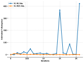
(a) KL (Office-31)

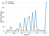
(b) KL (Office-Home)

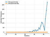
(c) $\chi^{2}$ (Office-31)

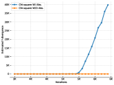
(d) $\chi^{2}$ (Office-Home)

Figure 2: Comparison between $\mathrm{D}_{\phi}^{h,\mathcal{H}}$ and $\widetilde{\mathrm{D}}_{\phi}^{h,\mathcal{H}}$. The $y$-axis is the estimated corresponding $f$-divergence and the $x$-axis is the number of iterations.

Table 9: Comparison between $\chi^{2}$-DD and Opt$\chi^{2}$-DD

Method	A$\to$D	Ar$\to$Cl
$\chi^{2}$-DD	95.0$\pm$0.4	55.2$\pm$0.3
Opt$\chi^{2}$-DD	93.1$\pm$0.3	53.9$\pm$0.3

Details and Additional Results for Optimal $f$-DD

As outlined in Section 6, instead of invoking a stochastic gradient-based optimizer (e.g., SGD) to update $t$, we utilize a quadratic approximation for the optimal $t$ as presented in Birrell et al. (2022). The approximately optimal KL-DD (OptKL-DD) is expressed as follows:

$$\mathrm{D}_{\rm KL}^{h,\mathcal{H}}(\nu||\mu)=\sup_{h^{\prime}}\left(1+\Delta t^{*}\right){{\mathbb{E}_{\nu}}\left[\ell(h,h^{\prime})\right]}-\log{{\mathbb{E}_{\mu}}\left[e^{\left(1+\Delta t^{*}\right)\ell(h,h^{\prime})}\right]}.$$

Here, a Gibbs measure is defined as $d\mu^{\prime}\triangleq\frac{e^{{\ell}(h,h^{\prime})}d\mu}{{{\mathbb{E}_{\mu}}\left[e^{{\ell}(h,h^{\prime})}\right]}}$, and $\Delta t^{*}$ is determined by the formula

$$\Delta t^{*}=\frac{{{\mathbb{E}_{\nu}}\left[{\ell}(h,h^{\prime})\right]}-{{\mathbb{E}_{\mu^{\prime}}}\left[\ell(h,h^{\prime})\right]}}{\mathrm{Var}_{\mu^{\prime}}(\ell(h,h^{\prime}))}.$$

This approximation is obtained by Birrell et al. (2022) through a Taylor expansion around $t=1$, with additional details provided in their Appendix B. In our implementation of OptKL-DD, similar to KL-DD, we use $\hat{\ell}$ to replace $\ell$.

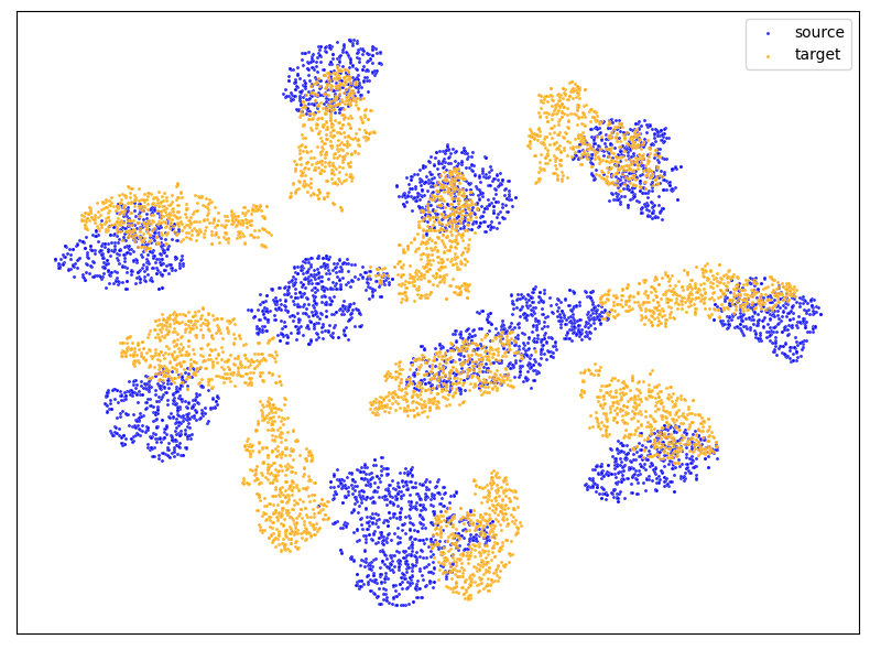
(a) $\chi^{2}$ in $f$-DAL

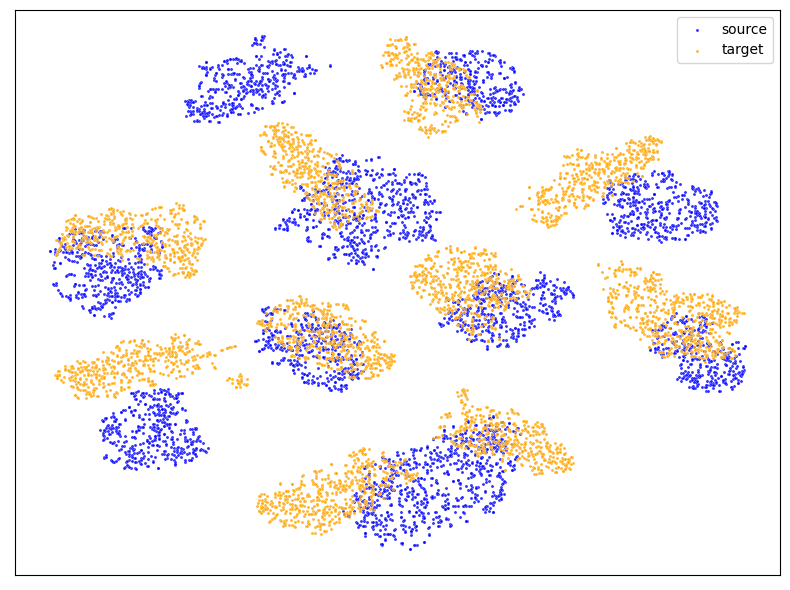
(b) $\chi^{2}$ in $f$-DD

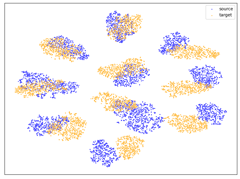
(c) KL-DD

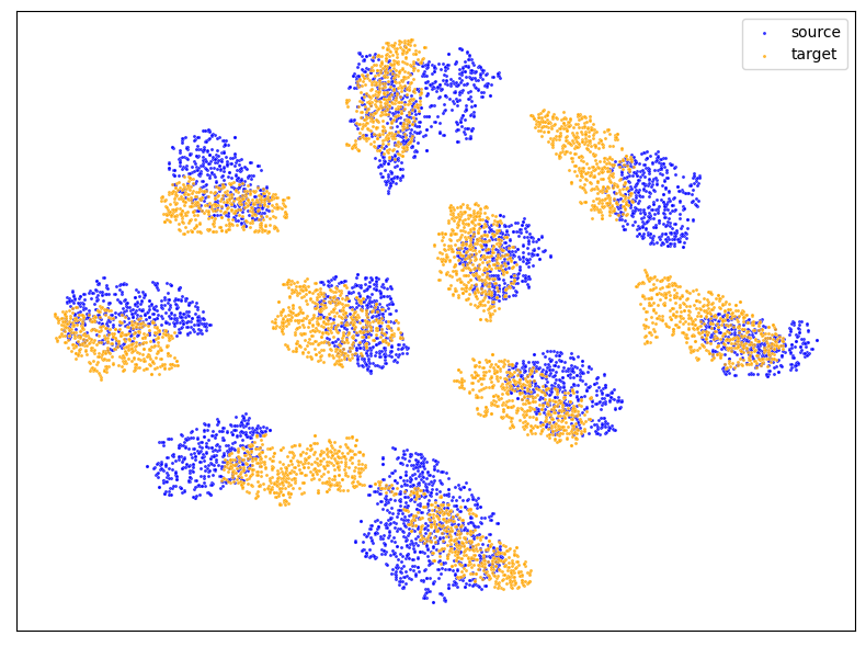
(d) Jeffereys-DD

Figure 3: Visualization results of representations obtained by using t-SNE. The source domain (blue points) is U and the target domain (orange points) is M.

For the optimal $\chi^{2}$-DD (Opt$\chi^{2}$-DD), we have its analytic form, as shown in Appendix C:

$$\mathrm{D}_{\chi^{2}}^{h,\mathcal{H}}(\nu||\mu)=\sup_{h^{\prime}}\frac{\left({{\mathbb{E}_{\nu}}\left[\ell(h,h^{\prime})\right]}-{{\mathbb{E}_{\mu}}\left[\ell(h,h^{\prime})\right]}\right)^{2}}{\mathrm{Var}_{\mu}\left(\ell(h,h^{\prime})\right)}.$$

By replacing $\ell$ by $\hat{\ell}$, we utilize the above as the training objective in our implementation. Table 9 illustrates that the optimal form does not improve performance in two sub-tasks, namely A$\to$D and Ar$\to$Cl, and in fact, may even degrade performance. Consequently, when the surrogate loss itself is unbounded, optimizing over $t$ may not be necessary, at least for $\chi^{2}$-DD and KL-DD.

Visualization Results

To visualize model representations (output of $h_{\rm rep}$) trained with $f$-DAL, $\chi^{2}$-DD, KL-DD, and Jeffereys-DD, we leverage t-SNE (Van der Maaten & Hinton, 2008). In Figure 3, we present visualization results using USPS (U) as the source domain and MNIST (M) as the target domain. Notably, while the original $f$-DAL already provides satisfactory results, our $f$-DD achieves further improvements in representation alignment.

References

- Acuna et al. (2021) Acuna, D., Zhang, G., Law, M. T., and Fidler, S. f-domain adversarial learning: Theory and algorithms. In International Conference on Machine Learning, pp. 66–75. PMLR, 2021.
- Agrawal & Horel (2020) Agrawal, R. and Horel, T. Optimal bounds between f-divergences and integral probability metrics. In International Conference on Machine Learning, pp. 115–124. PMLR, 2020.
- Agrawal & Horel (2021) Agrawal, R. and Horel, T. Optimal bounds between f-divergences and integral probability metrics. The Journal of Machine Learning Research, 22(1):5662–5720, 2021.
- Alquier (2021) Alquier, P. User-friendly introduction to pac-bayes bounds. arXiv preprint arXiv:2110.11216, 2021.
- Bartlett et al. (2005) Bartlett, P., Bousquet, O., and Mendelson, S. Local rademacher complexities. Annals of Statistics, 33(4):1497–1537, 2005.
- Bartlett & Mendelson (2002) Bartlett, P. L. and Mendelson, S. Rademacher and gaussian complexities: Risk bounds and structural results. Journal of Machine Learning Research, 3(Nov):463–482, 2002.
- Ben-David & Urner (2012) Ben-David, S. and Urner, R. On the hardness of domain adaptation and the utility of unlabeled target samples. In Algorithmic Learning Theory: 23rd International Conference, ALT 2012, Lyon, France, October 29-31, 2012. Proceedings 23, pp. 139–153. Springer, 2012.
- Ben-David et al. (2006) Ben-David, S., Blitzer, J., Crammer, K., and Pereira, F. Analysis of representations for domain adaptation. Advances in neural information processing systems, 19, 2006.
- Ben-David et al. (2010) Ben-David, S., Blitzer, J., Crammer, K., Kulesza, A., Pereira, F., and Vaughan, J. W. A theory of learning from different domains. Machine Learning, 79(1-2):151–175, 2010.
- Ben-Tal & Teboulle (2007) Ben-Tal, A. and Teboulle, M. An old-new concept of convex risk measures: The optimized certainty equivalent. Mathematical Finance, 17(3):449–476, 2007.
- Birrell et al. (2022) Birrell, J., Katsoulakis, M. A., and Pantazis, Y. Optimizing variational representations of divergences and accelerating their statistical estimation. IEEE Transactions on Information Theory, 68(7):4553–4572, 2022.
- Boucheron et al. (2005) Boucheron, S., Bousquet, O., and Lugosi, G. Theory of classification: A survey of some recent advances. ESAIM: probability and statistics, 9:323–375, 2005.
- Breiman (2001) Breiman, L. Statistical modeling: The two cultures (with comments and a rejoinder by the author). Statistical science, 16(3):199–231, 2001.
- Bruns-Smith et al. (2022) Bruns-Smith, D., D’Amour, A., Feller, A., and Yadlowsky, S. Tailored overlap for learning under distribution shift. In NeurIPS 2022 Workshop on Distribution Shifts: Connecting Methods and Applications, 2022.
- Bu et al. (2022) Bu, Y., Aminian, G., Toni, L., Wornell, G. W., and Rodrigues, M. Characterizing and understanding the generalization error of transfer learning with gibbs algorithm. In International Conference on Artificial Intelligence and Statistics, pp. 8673–8699. PMLR, 2022.
- Catoni (2007) Catoni, O. Pac-bayesian supervised classification: the thermodynamics of statistical learning. Vol. 56. Lecture Notes - Monograph Series. Institute of Mathematical Statistics, 2007.
- Cortes et al. (2015) Cortes, C., Mohri, M., and Muñoz Medina, A. Adaptation algorithm and theory based on generalized discrepancy. In Proceedings of the 21th ACM SIGKDD International Conference on Knowledge Discovery and Data Mining, pp. 169–178, 2015.
- Courty et al. (2017) Courty, N., Flamary, R., Habrard, A., and Rakotomamonjy, A. Joint distribution optimal transportation for domain adaptation. Advances in neural information processing systems, 30, 2017.
- Crooks (2008) Crooks, G. E. Inequalities between the jenson-shannon and jeffreys divergences. In Tech. Note 004, 2008.
- Deng et al. (2009) Deng, J., Dong, W., Socher, R., Li, L.-J., Li, K., and Fei-Fei, L. Imagenet: A large-scale hierarchical image database. In 2009 IEEE conference on computer vision and pattern recognition, pp. 248–255, 2009.
- Dhouib & Maghsudi (2022) Dhouib, S. and Maghsudi, S. Connecting sufficient conditions for domain adaptation: source-guided uncertainty, relaxed divergences and discrepancy localization. arXiv preprint arXiv:2203.05076, 2022.
- Donsker & Varadhan (1983) Donsker, M. D. and Varadhan, S. S. Asymptotic evaluation of certain markov process expectations for large time. iv. Communications on pure and applied mathematics, 36(2):183–212, 1983.
- Fisher et al. (2019) Fisher, A., Rudin, C., and Dominici, F. All models are wrong, but many are useful: Learning a variable’s importance by studying an entire class of prediction models simultaneously. J. Mach. Learn. Res., 20(177):1–81, 2019.
- Flamary et al. (2016) Flamary, R., Courty, N., Tuia, D., and Rakotomamonjy, A. Optimal transport for domain adaptation. IEEE Trans. Pattern Anal. Mach. Intell, 1(1-40):2, 2016.
- Ganin et al. (2016) Ganin, Y., Ustinova, E., Ajakan, H., Germain, P., Larochelle, H., Laviolette, F., Marchand, M., and Lempitsky, V. Domain-adversarial training of neural networks. The journal of machine learning research, 17(1):2096–2030, 2016.
- Germain et al. (2013) Germain, P., Habrard, A., Laviolette, F., and Morvant, E. A pac-bayesian approach for domain adaptation with specialization to linear classifiers. In International conference on machine learning, pp. 738–746. PMLR, 2013.
- Germain et al. (2016) Germain, P., Habrard, A., Laviolette, F., and Morvant, E. A new pac-bayesian perspective on domain adaptation. In International conference on machine learning, pp. 859–868. PMLR, 2016.
- Gong et al. (2013) Gong, B., Grauman, K., and Sha, F. Connecting the dots with landmarks: Discriminatively learning domain-invariant features for unsupervised domain adaptation. In International conference on machine learning, pp. 222–230. PMLR, 2013.
- Goodfellow et al. (2014) Goodfellow, I., Pouget-Abadie, J., Mirza, M., Xu, B., Warde-Farley, D., Ozair, S., Courville, A., and Bengio, Y. Generative adversarial nets. Advances in neural information processing systems, 27, 2014.
- Hanneke & Kpotufe (2019) Hanneke, S. and Kpotufe, S. On the value of target data in transfer learning. Advances in Neural Information Processing Systems, 32, 2019.
- Hanneke et al. (2023) Hanneke, S., Kpotufe, S., and Mahdaviyeh, Y. Limits of model selection under transfer learning. arXiv preprint arXiv:2305.00152, 2023.
- He et al. (2016) He, K., Zhang, X., Ren, S., and Sun, J. Deep residual learning for image recognition. In Proceedings of the IEEE conference on computer vision and pattern recognition, pp. 770–778, 2016.
- Hellström & Durisi (2021) Hellström, F. and Durisi, G. Fast-rate loss bounds via conditional information measures with applications to neural networks. In 2021 IEEE International Symposium on Information Theory (ISIT), pp. 952–957. IEEE, 2021.
- Hellström & Durisi (2022) Hellström, F. and Durisi, G. A new family of generalization bounds using samplewise evaluated CMI. In Advances in Neural Information Processing Systems, 2022.
- Huang et al. (2006) Huang, J., Gretton, A., Borgwardt, K., Schölkopf, B., and Smola, A. Correcting sample selection bias by unlabeled data. Advances in neural information processing systems, 19, 2006.
- Hull (1994) Hull, J. J. A database for handwritten text recognition research. IEEE Transactions on pattern analysis and machine intelligence, 16(5):550–554, 1994.
- Jeffreys (1946) Jeffreys, H. An invariant form for the prior probability in estimation problems. Proceedings of the Royal Society of London. Series A. Mathematical and Physical Sciences, 186(1007):453–461, 1946.
- Jiang et al. (2020) Jiang, X., Lao, Q., Matwin, S., and Havaei, M. Implicit class-conditioned domain alignment for unsupervised domain adaptation. In International Conference on Machine Learning, pp. 4816–4827. PMLR, 2020.
- Jiao et al. (2017) Jiao, J., Han, Y., and Weissman, T. Dependence measures bounding the exploration bias for general measurements. In 2017 IEEE International Symposium on Information Theory (ISIT), pp. 1475–1479. IEEE, 2017.
- Kingma & Welling (2013) Kingma, D. P. and Welling, M. Auto-encoding variational bayes. arXiv preprint arXiv:1312.6114, 2013.
- LeCun et al. (1998) LeCun, Y., Bottou, L., Bengio, Y., and Haffner, P. Gradient-based learning applied to document recognition. Proceedings of the IEEE, 86(11):2278–2324, 1998.
- Long et al. (2018) Long, M., Cao, Z., Wang, J., and Jordan, M. I. Conditional adversarial domain adaptation. Advances in neural information processing systems, 31, 2018.
- Mansour et al. (2009a) Mansour, Y., Mohri, M., and Rostamizadeh, A. Domain adaptation: Learning bounds and algorithms. In The 22nd Conference on Learning Theory, 2009a.
- Mansour et al. (2009b) Mansour, Y., Mohri, M., and Rostamizadeh, A. Multiple source adaptation and the rényi divergence. In Proceedings of the Twenty-Fifth Conference on Uncertainty in Artificial Intelligence, pp. 367–374, 2009b.
- McDiarmid (1998) McDiarmid, C. Concentration, pp. 195–248. Springer Berlin Heidelberg, 1998.
- Mohri et al. (2018) Mohri, M., Rostamizadeh, A., and Talwalkar, A. Foundations of machine learning. MIT press, 2018.
- Nguyen et al. (2022) Nguyen, A. T., Tran, T., Gal, Y., Torr, P., and Baydin, A. G. KL guided domain adaptation. In International Conference on Learning Representations, 2022.
- Nguyen et al. (2010) Nguyen, X., Wainwright, M. J., and Jordan, M. I. Estimating divergence functionals and the likelihood ratio by convex risk minimization. IEEE Transactions on Information Theory, 56(11):5847–5861, 2010.
- Nowozin et al. (2016) Nowozin, S., Cseke, B., and Tomioka, R. f-gan: Training generative neural samplers using variational divergence minimization. Advances in neural information processing systems, 29, 2016.
- Polyanskiy & Wu (2023) Polyanskiy, Y. and Wu, Y. Information Theory: From Coding to Learning. Cambridge university press, 2023.
- Quionero-Candela et al. (2009) Quionero-Candela, J., Sugiyama, M., Schwaighofer, A., and Lawrence, N. D. Dataset Shift in Machine Learning. The MIT Press, 2009.
- Redko et al. (2020) Redko, I., Morvant, E., Habrard, A., Sebban, M., and Bennani, Y. A survey on domain adaptation theory. arXiv preprint arXiv:2004.11829, 2020.
- Ruderman et al. (2012) Ruderman, A., Reid, M. D., García-García, D., and Petterson, J. Tighter variational representations of f-divergences via restriction to probability measures. In Proceedings of the 29th International Coference on International Conference on Machine Learning, pp. 1155–1162, 2012.
- Saenko et al. (2010) Saenko, K., Kulis, B., Fritz, M., and Darrell, T. Adapting visual category models to new domains. In Proceedings of the 11th European conference on Computer vision: Part IV, pp. 213–226, 2010.
- Seldin et al. (2012) Seldin, Y., Laviolette, F., Cesa-Bianchi, N., Shawe-Taylor, J., and Auer, P. Pac-bayesian inequalities for martingales. IEEE Transactions on Information Theory, 58(12):7086–7093, 2012.
- Semenova et al. (2022) Semenova, L., Rudin, C., and Parr, R. On the existence of simpler machine learning models. In Proceedings of the 2022 ACM Conference on Fairness, Accountability, and Transparency, pp. 1827–1858, 2022.
- Shen et al. (2018) Shen, J., Qu, Y., Zhang, W., and Yu, Y. Wasserstein distance guided representation learning for domain adaptation. In Thirty-second AAAI conference on artificial intelligence, 2018.
- Shui et al. (2022) Shui, C., Chen, Q., Wen, J., Zhou, F., Gagné, C., and Wang, B. A novel domain adaptation theory with jensen–shannon divergence. Knowledge-Based Systems, 257:109808, 2022.
- Song & Ermon (2020) Song, J. and Ermon, S. Bridging the gap between f-gans and wasserstein gans. In International Conference on Machine Learning, pp. 9078–9087. PMLR, 2020.
- Sun & Saenko (2016) Sun, B. and Saenko, K. Deep coral: Correlation alignment for deep domain adaptation. In European conference on computer vision, pp. 443–450. Springer, 2016.
- Sun et al. (2016) Sun, B., Feng, J., and Saenko, K. Return of frustratingly easy domain adaptation. In Proceedings of the AAAI conference on artificial intelligence, 2016.
- Tao et al. (2018) Tao, C., Chen, L., Henao, R., Feng, J., and Duke, L. C. generative adversarial network. In International conference on machine learning, pp. 4887–4896. PMLR, 2018.
- Tolstikhin & Seldin (2013) Tolstikhin, I. O. and Seldin, Y. Pac-bayes-empirical-bernstein inequality. Advances in Neural Information Processing Systems, 26, 2013.
- Van der Maaten & Hinton (2008) Van der Maaten, L. and Hinton, G. Visualizing data using t-sne. Journal of machine learning research, 9(11), 2008.
- Venkateswara et al. (2017) Venkateswara, H., Eusebio, J., Chakraborty, S., and Panchanathan, S. Deep hashing network for unsupervised domain adaptation. In Proceedings of the IEEE conference on computer vision and pattern recognition, pp. 5018–5027, 2017.
- Wang & Mao (2023a) Wang, Z. and Mao, Y. Information-theoretic analysis of unsupervised domain adaptation. In International Conference on Learning Representations, 2023a.
- Wang & Mao (2023b) Wang, Z. and Mao, Y. Sample-conditioned hypothesis stability sharpens information-theoretic generalization bounds. In Advances in Neural Information Processing Systems, 2023b.
- Wang & Mao (2023c) Wang, Z. and Mao, Y. Tighter information-theoretic generalization bounds from supersamples. In International Conference on Machine Learning. PMLR, 2023c.
- Wu et al. (2020) Wu, X., Manton, J. H., Aickelin, U., and Zhu, J. Information-theoretic analysis for transfer learning. In 2020 IEEE International Symposium on Information Theory (ISIT), pp. 2819–2824. IEEE, 2020.
- Wu et al. (2019) Wu, Y., Winston, E., Kaushik, D., and Lipton, Z. Domain adaptation with asymmetrically-relaxed distribution alignment. In International conference on machine learning, pp. 6872–6881. PMLR, 2019.
- Yang et al. (2019) Yang, J., Sun, S., and Roy, D. M. Fast-rate pac-bayes generalization bounds via shifted rademacher processes. Advances in Neural Information Processing Systems, 32, 2019.
- Zhang et al. (2019) Zhang, Y., Liu, T., Long, M., and Jordan, M. Bridging theory and algorithm for domain adaptation. In International Conference on Machine Learning, pp. 7404–7413. PMLR, 2019.
- Zhang et al. (2020) Zhang, Y., Long, M., Wang, J., and Jordan, M. I. On localized discrepancy for domain adaptation. arXiv preprint arXiv:2008.06242, 2020.