$\sigma$-zero: Gradient-based Optimization of $\ell_{0}$-norm
Adversarial Examples

Abstract

Evaluating the adversarial robustness of deep networks to gradient-based attacks is challenging. While most attacks consider $\ell_{2}$- and $\ell_{\infty}$-norm constraints to craft input perturbations, only a few investigate sparse $\ell_{1}$- and $\ell_{0}$-norm attacks. In particular, $\ell_{0}$-norm attacks remain the least studied due to the inherent complexity of optimizing over a non-convex and non-differentiable constraint. However, evaluating adversarial robustness under these attacks could reveal weaknesses otherwise left untested with more conventional $\ell_{2}$- and $\ell_{\infty}$-norm attacks. In this work, we propose a novel $\ell_{0}$-norm attack, called $\sigma$-zero, which leverages an ad hoc differentiable approximation of the $\ell_{0}$ norm to facilitate gradient-based optimization, and an adaptive projection operator to dynamically adjust the trade-off between loss minimization and perturbation sparsity. Extensive evaluations using MNIST, CIFAR10, and ImageNet datasets, involving robust and non-robust models, show that $\sigma$-zero finds minimum $\ell_{0}$-norm adversarial examples without requiring any time-consuming hyperparameter tuning, and that it outperforms all competing sparse attacks in terms of success rate, perturbation size, and scalability.
Code available at: https://github.com/Cinofix/sigma-zero-adversarial-attack

I Introduction

Early research has revealed that machine learning models are fooled by adversarial examples, i.e., carefully perturbed inputs optimized to cause misclassifications (Biggio et al., 2013; Szegedy et al., 2014). In turn, this has demanded more careful reliability assessments of such models. Most of the gradient-based attacks proposed to evaluate the adversarial robustness of Deep Neural Networks (DNNs) optimize adversarial examples under different $\ell_{p}$-norm constraints. In particular, while convex $\ell_{1}$, $\ell_{2}$, and $\ell_{\infty}$ norms have been widely studied (Chen et al., 2018; Croce and Hein, 2021a), only a few $\ell_{0}$-norm attacks have been considered to date. The main reason is that ad-hoc heuristics need to be adopted to compute efficient projections on the $\ell_{0}$ norm, overcoming issues related to its non-convexity and non-differentiability. Although this task is challenging and computationally expensive, attacks based on the $\ell_{0}$ norm have the potential to reveal uncovered issues in DNNs that may not be evident in other norm-based attacks (Carlini and Wagner, 2017a; Croce and Hein, 2021a). For instance, these attacks, known to perturb a minimal fraction of input features, can be used to determine the most sensitive characteristics that influence the model’s decision-making process. Furthermore, they offer a different and relevant threat model to benchmark existing defenses. Developing efficient algorithms for generating $\ell_{0}$-norm adversarial examples is thus a crucial area of research that requires further exploration to improve current adversarial robustness evaluations.

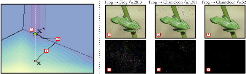
Figure 1: The leftmost plot shows an instance of $\mathtt{\sigma}$-zero’s execution on a two-dimensional problem. The initial point $\bm{\mathbf{x}}$ (red dot) is modified via gradient descent to find the adversarial example $\bm{\mathbf{x}}^{\star}$ (green star) while minimizing the number of perturbed features (i.e., the $\ell_{0}$ norm of the perturbation). The gray lines surrounding $\bm{\mathbf{x}}$ demarcate regions where the $\ell_{0}$ norm is minimized. The rightmost plot shows the adversarial images (top row) and the corresponding perturbations (bottom row) found by $\mathtt{\sigma}$-zero during the three steps highlighted in the leftmost plot, alongside their prediction and $\ell_{0}$ norm.

Unfortunately, current implementations of $\ell_{0}$-norm attacks exhibit a largely suboptimal trade-off between their success rate and efficiency, that is, they are either accurate but slow or fast but inaccurate. In particular, the accurate ones use complex projections to find smaller input perturbations but suffer from time or memory limitations, hindering their scalability to larger networks or high-dimensional data (Brendel et al., 2019a; Césaire et al., 2021). Other attacks execute faster, but their output solution is typically inaccurate and largely suboptimal, as they rely on heuristic approaches and imprecise approximations to bypass the difficulties of optimizing the $\ell_{0}$ norm, leading to overestimating adversarial robustness (Matyasko and Chau, 2021; Pintor et al., 2021). Therefore, it remains an open challenge to develop a scalable and compelling method to assess the robustness of DNNs against sparse perturbations with minimum $\ell_{0}$ norm.

In this work, we propose a novel $\ell_{0}$-norm attack, named $\mathtt{\sigma}$-zero, which iteratively promotes the sparsity of the adversarial perturbation by minimizing its $\ell_{0}$ norm (see Fig. 1 and Sect. II). To overcome the limitations of previous approaches, we design our attack based on two main technical contributions. First, we use an unbiased, differentiable approximation of the $\ell_{0}$ norm, originally proposed by Osborne et al. (2000a), to enable the minimization of the attack loss function via gradient descent. Second, we introduce an adaptive projection operator that dynamically adjusts a sparsity threshold to reduce the perturbation size while keeping the perturbed sample in the adversarial region.

Our experiments (Sect. III) provide compelling evidence of the remarkable performance of $\mathtt{\sigma}$-zero. We evaluate it on several benchmark datasets, including MNIST, CIFAR10, and ImageNet, considering baseline and robust models from Robustbench (Croce et al., 2021). We compare its performance with competing attacks, showing that $\mathtt{\sigma}$-zero achieves better results in terms of attack success rate and perturbation size, while being significantly faster and without requiring sophisticated and time-consuming hyperparameter tuning. We firmly believe that $\mathtt{\sigma}$-zero will foster significant advancements in the development of better robustness evaluation tools and more robust models. We conclude the paper by discussing related work (Sect. IV), along with the main contributions and future directions to address the limitations of the proposed approach (Sect. V).

II $\mathtt{\sigma}$-zero: Minimum $\ell_{0}$-norm Attacks

We present here $\mathtt{\sigma}$-zero, our gradient-based approach to finding minimum $\ell_{0}$-norm adversarial examples. We start by describing the threat model and then give a formal overview of the proposed attack and its algorithmic implementation.

Threat Model. We assume that the attacker has complete access to the target model, including its architecture and trained parameters, and exploits its gradient for staging white-box untargeted attacks (Carlini and Wagner, 2017a; Biggio and Roli, 2018). This setting is useful for worst-case evaluation of the adversarial robustness of DNNs, providing empirical upper bounds on the performance degradation that may be incurred under attack. Note that this is the standard setting adopted in previous work for gradient-based adversarial robustness evaluations (Carlini and Wagner, 2017a; Brendel et al., 2019b; Croce et al., 2021; Pintor et al., 2021).

Problem Formulation. In this work, we seek untargeted minimum $\ell_{0}$-norm adversarial perturbations that steer the model’s decision towards misclassification (Carlini and Wagner, 2017a). To this end, let $\bm{\mathbf{x}}\in\mathcal{X}=[0,1]^{d}$ be a $d$-dimensional input sample, $y\in\mathcal{Y}=\{1,\ldots,l\}$ its associated true label, and $f:\mathcal{X}\times\Theta\mapsto\mathcal{Y}$ the target model, parameterized by $\bm{\mathbf{\theta}}\in\Theta$. While $f$ outputs the predicted label, we will also use $f_{k}$ to denote the continuous-valued output (logit) for class $k\in\mathcal{Y}$. The goal of our attack is to find the minimum $\ell_{0}$-norm adversarial perturbation $\bm{\mathbf{\delta}}^{\star}$ such that the corresponding adversarial example $\bm{\mathbf{x}}^{\star}=\bm{\mathbf{x}}+\bm{\mathbf{\delta}}^{\star}$ is misclassified by $f$. This can be formalized as:

$$\bm{\mathbf{\delta}}^{\star}\in\arg\min_{\bm{\mathbf{\delta}}} \|\bm{\mathbf{\delta}}\|_{0}\,,$$ (1)

s.t. $$f(\bm{\mathbf{x}}+\bm{\mathbf{\delta}},\bm{\mathbf{\theta}})\neq y\,,$$ (3)

$$\bm{\mathbf{x}}+\bm{\mathbf{\delta}}\in[0,1]^{d}\,,$$

where $\|\cdot\|_{0}$ denotes the $\ell_{0}$ norm, which counts the number of non-zero dimensions. The hard constraint in Equation 3 ensures that the perturbation $\bm{\mathbf{\delta}}$ is valid only if it induces the target model $f$ to misclassify the perturbed sample $\bm{\mathbf{x}}+\bm{\mathbf{\delta}}$. Similarly, Equation 3, which represents a box constraint, ensures that the perturbed sample $\bm{\mathbf{x}}+\bm{\mathbf{\delta}}$ lies in $[0,1]^{d}$. Note that, when the source point $\bm{\mathbf{x}}$ is already misclassified by $f$, the solution to the above minimization problem is $\bm{\mathbf{\delta}}^{\star}=\bm{\mathbf{0}}$.

Since Problem (1)-(3) cannot be solved directly, we reformulate it here as:

$$\bm{\mathbf{\delta}}^{\star}\in\arg\min_{\bm{\mathbf{\delta}}} \mathcal{L}(\bm{\mathbf{x}}+\bm{\mathbf{\delta}},y,\bm{\mathbf{\theta}})+\frac{1}{d}\hat{\ell}_{0}(\bm{\mathbf{\delta}})$$ (4)

s.t. $$\bm{\mathbf{x}}+\bm{\mathbf{\delta}}\in[0,1]^{d}\,,~{}$$ (5)

where we use a differentiable approximation $\hat{\ell}_{0}(\bm{\mathbf{\delta}})$ instead of $||\bm{\mathbf{\delta}}||_{0}$, and normalize it with respect to the number of features $d$ to ensure that its value is within the interval $[0,1]$, as described in the next paragraph. The loss $\mathcal{L}$ is defined as:

$$\mathcal{L}(\bm{\mathbf{x}},y,\bm{\mathbf{\theta}})=\max\left(f_{y}(\bm{\mathbf{x}},\bm{\mathbf{\theta}})-\max_{k\neq y}f_{k}(\bm{\mathbf{x}},\bm{\mathbf{\theta}}),0\right)\\ +\mathbb{I}(f(\bm{\mathbf{x}},\bm{\mathbf{\theta}})=y)\,.$$ (6)

The first term in $\mathcal{L}$ represents the logit difference, which is positive when the sample is correctly assigned to the true class $y$, and clipped to zero when it is misclassified (Carlini and Wagner, 2017a). The second term merely adds $1$ to the loss if the sample is correctly classified. This ensures that the loss term $\mathcal{L}$ is $0$ only when an adversarial example is found and higher than $1$ otherwise. This, in turn, implies that the loss term $\mathcal{L}$ is always higher than the $\ell_{0}$-norm term in Equation 4 (as the latter is bounded in $[0,1]$), when no adversarial example is found. Accordingly, it is not difficult to see that the feasible solutions to this problem correspond only to minimum-norm adversarial examples. It is also worth remarking that, conversely to the objective function proposed by Carlini and Wagner (2017a), our objective does not require tuning any trade-off hyperparameters to balance between minimizing the loss and reducing the perturbation size, thus avoiding a computationally expensive line search for each input sample. In fact, the proposed objective function inherently induces an alternate optimization process between the loss term and the $\ell_{0}$-norm penalty, as shown in the appendix (see Figure 3). In particular, when the sample is not adversarial, the attack algorithm mostly aims to decrease the loss term to find an adversarial example while increasing the perturbation size. Conversely, when an adversarial example is found, the loss term is cropped to zero, and the perturbation size is gradually reduced.

$\ell_{0}$-norm Approximation. Besides the formalization of the attack objective, one of the main technical advantages of $\mathtt{\sigma}$-zero is to use an appropriate, differentiable approximation of the $\ell_{0}$ norm, thereby enabling the use of gradient-based optimization. To this end, we leverage the $\ell_{0}$-norm approximation originally proposed by Osborne et al. (2000a):

$$\hat{\ell}_{0}(\bm{\mathbf{x}},\sigma)=\sum\limits_{i=1}^{d}\frac{x_{i}^{2}}{x_{i}^{2}+\sigma}, \sigma>0, \hat{\ell}_{0}(\bm{\mathbf{x}},\sigma)\in[0,d]\,,$$ (7)

where $\sigma$ is a hyperparameter controlling the smoothness of the approximation. When $\sigma$ tends to zero, the approximation becomes more accurate but less smooth, potentially leading to the same optimization limits of the $\ell_{0}$ norm. In our experiments, we find that fixing $\sigma=10^{-3}$ provides good results, without requiring any additional tuning.

Adaptive Projection Operator $\Pi_{\tau}$. The considered $\ell_{0}$-norm approximation allows $\mathtt{\sigma}$-zero to use standard gradient descent to optimize Equation 4. However, this approximation promotes solutions that are not fully sparse, i.e., with many components that are very close to zero but not exactly equal to zero, thereby yielding over-inflated $\ell_{0}$-norm values. To overcome this issue, we introduce an adaptive projection operator $\Pi_{\tau}$ that sets to zero the features with a perturbation intensity lower than a given sparsity threshold $\tau$ in each iteration. The sparsity threshold $\tau$ is initialized with a starting value $\tau_{0}$ and then dynamically adjusted for each sample during each iteration; in particular, it is increased to find sparser perturbations when the current sample is already adversarial, while it is decreased otherwise, allowing larger perturbations to help find an adversarial example. The updates to $\tau$ are proportional to the step size, and follow its annealing strategy, as detailed below.

Solution Algorithm. We present here our gradient-based algorithm for solving Problem (4)-(5). Our attack, described in Algorithm 1, is fast, memory efficient, and easy to implement. After initializing the adversarial perturbation $\bm{\mathbf{\delta}}=\bm{\mathbf{0}}$ (algorithm 1), it computes the gradient of the objective in Equation 4 with respect to $\bm{\mathbf{\delta}}$ (algorithm 1). The gradient is then normalized (algorithm 1) to stabilize the optimization by making the update independent from the gradient size (Rony et al., 2018; Pintor et al., 2021). In particular, the gradient is divided by its $\ell_{\infty}$ norm to avoid any dependency between the step size and the dimensionality of the input data, given that the $\ell_{\infty}$ norm is not affected by changes in the input dimensionality. We then update $\bm{\mathbf{\delta}}$ to minimize the objective via gradient descent, while also enforcing the box constraints in Equation 5 through the usage of the clip operator (algorithm 1). We increase sparsity in $\bm{\mathbf{\delta}}$ by zeroing all components lower than the current sparsity threshold $\tau$ (algorithm 1), as discussed in the previous paragraph. We then decrease the step size $\eta$ by following a cosine-annealing schedule (algorithm 1), as suggested by Rony et al. (2018); Pintor et al. (2021), and adjust the sparsity threshold $\tau$ dynamically (algorithm 1). In particular, if the current sample is adversarial, we increase $\tau$ by $1\%\eta$ to promote sparser perturbations; otherwise, we decrease $\tau$ by the same amount to promote the minimization of $\mathcal{L}$. The above process is repeated for $N$ iterations while keeping track of the best solution found so far, i.e., the adversarial perturbation $\bm{\mathbf{\delta}}^{\star}$ with the lowest $\ell_{0}$ norm (algorithm 1). If no adversarial example is found, the algorithm sets $\bm{\mathbf{\delta}}^{\star}=\infty$ (algorithm 1). It terminates by returning $\bm{\mathbf{x}}^{\star}=\bm{\mathbf{x}}+\bm{\mathbf{\delta}}^{\star}$ (algorithm 1).

Remarks. To summarize, the main contributions behind $\mathtt{\sigma}$-zero are: (i) the use of a differentiable approximation for the $\ell_{0}$ norm Osborne et al. (2000a) to design a novel loss function (Equation 4) that simultaneously enables the search for adversarial examples and the minimization of the $\ell_{0}$ norm of the perturbation (i.e., a non-trivial task given the non-convexity of this norm); and (ii) the introduction of an adaptive projection operator that dynamically enforces sparsity into the adversarial perturbations. Our novel formulation, together with some optimization tricks (i.e., gradient normalization and step size annealing), yields a fast and reliable $\ell_{0}$-norm attack that does not even require extensive hyperparameter tuning, as reported in Appendix B-B.

Input: $\bm{\mathbf{x}}\in[0,1]^{d}$, the input sample; y, the true class label; $\bm{\mathbf{\theta}}$, the target model; N, the number of iterations; $\sigma$, the $\ell_{0}$-norm approximation hyperparameter; $\eta_{0}$, the initial step size; $\tau_{0}$, the initial sparsity threshold.

Output: $\bm{\mathbf{x}}^{\star}$, the minimum $\ell_{0}$-norm adversarial example.

1 $\bm{\delta}\leftarrow\bm{\mathbf{0}}$; $\quad\bm{\mathbf{\delta}}^{\star}\leftarrow\bm{\mathbf{0}}$; $\quad\tau\leftarrow\tau_{0}$; $\quad\eta\leftarrow\eta_{0}$

2for i in $1,\dots,N$ do

3      

4      $\nabla\bm{\mathbf{g}}\leftarrow\nabla_{\bm{\mathbf{\delta}}}[\mathcal{L}(\bm{\mathbf{x}}+\bm{\mathbf{\delta}},y,\bm{\mathbf{\theta}})+\frac{1}{d}\hat{\ell}_{0}(\bm{\mathbf{\delta}},\sigma)]$

5      $\nabla\bm{\mathbf{g}}\leftarrow{\nabla\bm{\mathbf{g}}}/{\|\nabla\bm{\mathbf{g}}\|_{\infty}}$

6      $\bm{\mathbf{\delta}}\leftarrow$ clip$(\bm{\mathbf{x}}-[\bm{\mathbf{\delta}}-\eta\cdot\nabla\bm{\mathbf{g}}])-\bm{\mathbf{x}}$ 

7      $\bm{\mathbf{\delta}}\leftarrow\Pi_{\tau}(\bm{\mathbf{\delta}})$

8      $\eta=\texttt{cosine\_annealing}(\eta_{0},i)$

9      if $\mathcal{L}(\bm{\mathbf{x}}+\bm{\mathbf{\delta}},y,\bm{\mathbf{\theta}})\leq 0$: $\tau+=0.01\cdot\eta$, else $\tau-=0.01\cdot\eta$

10      if $\mathcal{L}(\bm{\mathbf{x}}+\bm{\mathbf{\delta}},y,\bm{\mathbf{\theta}})\leq 0~{}\wedge~{}\|\bm{\mathbf{\delta}}\|_{0}<\|\bm{\mathbf{\delta}}^{\star}\|_{0}$: $\bm{\mathbf{\delta}}^{\star}\leftarrow\bm{\mathbf{\delta}}$

11 end for

12

13if $\mathcal{L}(\bm{\mathbf{x}}+\bm{\mathbf{\delta}}^{\star},y,\bm{\mathbf{\theta}})>0$: $\bm{\mathbf{\delta}}^{\star}\leftarrow\infty$

return $\bm{\mathbf{x}}^{\star}\leftarrow\bm{\mathbf{x}}+\bm{\mathbf{\delta}}^{\star}$

Algorithm 1 $\mathtt{\sigma}$-zero Attack Pseudocode.

III Experiments

We report here an extensive experimental evaluation comparing $\mathtt{\sigma}$-zero against 9 state-of-the-art sparse attacks, including both $\ell_{0}$- and $\ell_{1}$-norm attacks. We test all attacks using different settings on 16 distinct models and 3 different datasets, yielding almost 400 different comparisons in total.

III-A Experimental Setup

Datasets. We consider the three most popular datasets used for benchmarking adversarial robustness: MNIST (LeCun and Cortes, 2005), CIFAR10 (Krizhevsky, 2009) and ImageNet (Krizhevsky et al., 2012). To evaluate the attack performance, we use the entire test set for MNIST and CIFAR10 (with a batch size of 32), and a subset of $1000$ test samples for ImageNet (with a batch size of 16).

Models. We use a selection of both baseline and robust models to evaluate the attacks under different conditions. Our goal is to compare $\mathtt{\sigma}$-zero on a vast set of models to ensure its broad effectiveness and to expose vulnerabilities that may not be revealed by other attacks (Croce and Hein, 2021a). For the MNIST dataset, we consider two adversarially trained convolutional neural network (CNN) models by Rony et al. (2021a), i.e., CNN-DDN and CNN-Trades. These models have been trained to be robust to both $\ell_{2}$ and $\ell_{\infty}$ adversarial attacks. We denote them M1 and M2, respectively. For the CIFAR10 and ImageNet datasets, we employ state-of-the-art robust models from RobustBench (Croce et al., 2021). For CIFAR10, we adopt ten models, denoted as C1-C10. C1 (Croce et al., 2021) is a non-robust WideResNet-28-10 model. C2 (Carmon et al., 2019) and C3 (Augustin et al., 2020) combine training data augmentation with adversarial training to improve robustness to $\ell_{\infty}$ and $\ell_{2}$ attacks. C4 (Engstrom et al., 2019) is an adversarially trained model that is robust against $\ell_{2}$-norm attacks. C6 (Gowal et al., 2021) exploits generative models to artificially augment the original training set and improve adversarial robustness to generic $\ell_{p}$-norm attacks. C7 (Chen et al., 2020) is a robust ensemble model. C8 (Xu et al., 2023) is a recently proposed adversarial training defense robust to $\ell_{2}$ attacks. C9 (Addepalli et al., 2022) enforces diversity during data augmentation and combines it with adversarial training. Finally, we include the $\ell_{1}$ robust models C5 (Croce and Hein, 2021b) and C10 (Jiang et al., 2023). For ImageNet, we consider a pretrained ResNet-18 denoted with I1 (He et al., 2015), and five robust models to $\ell_{\infty}$-attacks, denoted with I2 (Engstrom et al., 2019), I3 (Wong et al., 2020), I4 (Salman et al., 2020), I5 (Hendrycks et al., 2021), and I6 (Salman et al., 2020).

Attacks. We compare $\mathtt{\sigma}$-zero against the following state-of-the-art minimum-norm attacks, in their $\ell_{0}$-norm variants: the Voting Folded Gaussian Attack (VFGA) attack (Césaire et al., 2021), the Primal-Dual Proximal Gradient Descent (PDPGD) attack (Matyasko and Chau, 2021), the Brendel & Bethge (BB) attack (Brendel et al., 2019a), including also its variant with adversarial initialization (BBadv), and the Fast Minimum Norm (FMN) attack (Pintor et al., 2021). We also consider two state-of-the-art $\ell_{1}$-norm attacks as additional baselines, that is, the Elastic-Net (EAD) attack (Chen et al., 2018) and SparseFool (Modas et al., 2019), along with two further $\ell_{0}$-norm attacks, i.e., the $\ell_{0}$-norm Projected Gradient Descent (PGD-$\ell_{0}$) attack (Croce and Hein, 2019) and the Sparse Random Search (Sparse-RS) attack (Croce et al., 2022). We configure all attacks to manipulate the input values independently without constraining the manipulations on individual pixels Croce et al. (2022); e.g., for CIFAR10, the number of modifiable inputs is thus $3\times 32\times 32=3072$. In contrast to minimum-norm attacks, the fixed-budget attacks PGD-$\ell_{0}$ and Sparse-RS aim to maximize misclassification confidence within a maximum number of modifiable features $k$. Thus, to ensure a fair comparison with minimum-norm attacks, as done by Rony et al. (2021b), we consider their perturbation budget $k$ as a hyperparameter and minimize it through a sample-wise binary search. In this case, we perform 10 iterations of line search over $k$, and for each value of $k$ we run the attack for $N/10$ iterations so that the overall number of steps remains $N$. Additional details can be found in Appendix C-B, along with supplementary experiments that show how $\mathtt{\sigma}$-zero outperforms both PGD-$\ell_{0}$ and Sparse-RS even when they use all the $N$ iterations to optimize the attacks with a fixed $k$.

Hyperparameters. We run our experiments using the default hyperparameters used in the original implementation of the attacks from AdversarialLib (Rony and Ben Ayed, ) and Foolbox (Rauber et al., 2017). We only change the maximum number of iterations to $N=1000$ to ensure that all attacks reach convergence (Pintor et al., 2022). We report additional results using only $N=100$ steps in Appendix C-A. For gradient-based attacks, one iteration amounts to performing at least one forward and one backward pass. Thus, to ensure a fairer comparison with Sparse-RS, which performs only one forward pass per iteration, we run it using $N=4000$ and $N=400$ in the two distinct configurations. For $\mathtt{\sigma}$-zero, we set $\eta_{0}=1$, $\tau_{0}=0.3$ and $\sigma=10^{-3}$, and keep the same configuration for all models and datasets, to show that no specific hyperparameter tuning is required. Additional analyses of the influence of the hyperparameters on the performance of $\mathtt{\sigma}$-zero can be found in Appendix B-B.

Evaluation Metrics. For each attack, we report the Attack Success Rate at different values of $k$, denoted with ASR_k, i.e., the fraction of successful attacks for which $\|\bm{\mathbf{\delta}}^{\star}\|_{0}\leq k$, and the median value of $\|\bm{\mathbf{\delta}}^{\star}\|_{0}$ over the test samples, denoted with $\tilde{\ell}_{0}$. We compare the computational effort of each attack considering the mean runtime (per sample), the mean number of queries (i.e., the total number of forwards and backwards required to perform the attack, divided by the number of samples), and the Video Random Access Memory (VRAM) consumed by the Graphics Processing Unit (GPU). We measure the runtime on a workstation with an NVIDIA A100 Tensor Core GPU (40 GB memory) and two Intel^® Xeo^® Gold 6238R processors. We evaluate memory consumption as the maximum amount of VRAM used by each attack among all batches, which is the minimum requirement to run it without failures.

III-B Experimental Results

We report the performance and computational effort metrics for all attacks and model-dataset settings in Tables I-III.

TABLE I: Results on MNIST with $N=1000$. For each attack and model (M), we report ASR at $k=10,50,\infty$, median perturbation size $\mathbf{\tilde{\ell}}_{0}$, mean runtime $t$ (in seconds), mean number of queries $q$ ($\div$ 1000), and maximum VRAM usage (in GB).

Attack	M	ASR10	ASR50	ASR∞	$\mathbf{\tilde{\ell}}_{0}$	$\mathbf{t}$	$\mathbf{q}$	VRAM	M	ASR10	ASR50	ASR∞	$\mathbf{\tilde{\ell}}_{0}$	$\mathbf{t}$	$\mathbf{q}$	VRAM
EAD		1.14	53.66	100.0	49	0.47	6.28	0.05		1.20	55.57	100.0	48	0.50	6.73	0.05
VFGA		9.62	82.42	99.98	27	0.05	0.77	0.21		1.80	39.33	99.95	57	0.05	1.33	0.21
PDPGD		2.97	74.08	100.0	38	0.23	2.00	0.04		3.31	66.30	100.0	42	0.23	2.00	0.04
BB		14.97	97.86	100.0	18	0.90	2.99	0.05		25.95	91.62	100.0	18	0.74	3.71	0.05
BBadv		14.81	91.23	100.0	19	0.77	2.01	0.07		14.42	40.88	100.0	89	0.71	2.01	0.07
PGD-$\ell_{0}$		12.22	99.84	100.0	19	1.15	1.99	0.07		5.04	90.17	100.0	24	1.42	2.00	0.06
Sparse-RS		12.57	83.74	100.0	25	4.55	3.05	0.07		59.73	98.59	100.0	9	3.53	2.44	0.06
SparseFool		4.86	6.76	96.98	469	1.07	0.18	0.06		0.93	1.21	91.68	463	2.87	0.86	0.07
FMN		7.29	93.74	100.0	29	0.21	2.00	0.04		10.86	91.84	99.41	24	0.22	2.00	0.04
1-17 $\mathtt{\sigma}$-zero	M1	19.60	99.98	100.0	16	0.31	2.00	0.04	M2	61.57	100.0	100.0	9	0.31	2.00	0.04

TABLE II: Results for CIFAR10 with $N=1000$. See the caption of Table I for further details. When VFGA exceeds the VRAM limit, we re-run it using a smaller batch size, increasing its runtime $t$. We denote those cases with the symbol ‘$\star$’.

Attack	M	ASR10	ASR50	ASR∞	$\mathbf{\tilde{\ell}}_{0}$	$\mathbf{t}$	$\mathbf{q}$	VRAM	M	ASR10	ASR50	ASR∞	$\mathbf{\tilde{\ell}}_{0}$	$\mathbf{t}$	$\mathbf{q}$	VRAM
EAD		6.74	21.33	100.0	126	2.32	6.90	1.47		14.47	35.90	100.0	74	10.76	5.55	9.92
VFGA		48.58	93.41	99.99	11	0.17	0.32	11.96		27.71	67.51	99.88	29	4.91⋆	1.02	> 40
PDPGD		16.58	78.97	100.0	27	0.64	2.00	1.31		17.68	40.89	100.0	69	3.96	2.00	8.86
BB		69.77	99.79	100.0	7	5.81	2.76	1.47		13.46	17.14	17.94	$\bm{{\color[rgb]{1,0,0}\infty}}$	3.46	2.08	9.93
BBadv		69.58	99.86	100.0	7	4.57	2.01	1.63		38.46	88.92	100.0	16	8.85	2.01	10.03
PGD-$\ell_{0}$		31.82	85.21	100.0	18	6.46	1.93	1.73		20.45	50.78	100.0	48	19.20	1.92	10.95
Sparse-RS		81.30	99.80	100.0	4	3.76	1.49	1.74		41.92	75.63	100.0	15	26.35	2.40	10.90
SparseFool		11.19	11.19	56.56	3072	1.42	0.37	1.57		16.74	16.79	35.38	$\bm{{\color[rgb]{1,0,0}\infty}}$	19.74	0.62	10.00
FMN		67.52	99.97	100.0	7	0.60	2.00	1.3		27.97	68.38	100.0	29	3.91	2.00	8.86
1-17 $\mathtt{\sigma}$-zero	C1	80.84	100.0	100.0	5	0.74	2.00	1.51	C6	48.38	94.47	100.0	11	4.41	2.00	10.43
EAD		12.70	30.38	100.0	90	1.92	5.70	1.47		17.29	33.68	100.0	105	8.33	5.37	5.39
VFGA		28.98	75.37	99.92	24	0.59	0.78	11.71		34.17	81.79	99.89	20	4.30⋆	0.62	> 40
PDPGD		16.47	42.50	100.0	63	0.64	2.00	1.32		21.37	48.96	99.82	51	2.15	2.00	5.12
BB		11.73	14.24	14.70	$\bm{{\color[rgb]{1,0,0}\infty}}$	0.63	2.05	1.47		37.98	78.76	83.58	16	12.49	3.14	5.39
BBadv		37.64	90.57	100.0	16	4.68	2.01	1.64		43.93	93.42	100.0	13	6.99	2.01	5.51
PGD-$\ell_{0}$		21.40	56.85	100.0	39	5.79	1.92	1.75		26.38	65.60	100.0	30	28.95	1.89	6.40
Sparse-RS		36.41	69.49	100.0	21	9.97	2.53	1.71		36.40	68.55	100.0	23	34.99	2.46	6.40
SparseFool		18.31	18.77	56.39	3072	11.31	1.40	1.62		23.67	24.85	62.41	3072	9.86	0.20	5.50
FMN		28.43	74.70	100.0	26	0.59	2.00	1.31		33.30	79.70	100.0	21	2.05	2.00	5.12
1-17 $\mathtt{\sigma}$-zero	C2	47.15	95.38	100.0	11	0.73	2.00	1.53	C7	52.46	97.33	100.0	10	2.75	2.00	5.90
EAD		9.21	11.42	100.0	360	2.53	5.62	1.89		9.38	23.62	100.0	148	2.23	5.80	2.15
VFGA		21.82	66.50	99.62	34	0.48	0.94	16.53		22.79	56.72	99.81	39	3.15⋆	1.84	> 40
PDPGD		13.96	45.15	100.0	55	1.12	2.00	1.8		11.97	38.41	100.0	69	0.76	2.00	2.0
BB		21.32	56.78	58.64	33	2.31	2.89	1.89		38.82	93.24	100.0	15	6.49	2.87	2.16
BBadv		31.64	96.31	100.0	17	3.92	2.01	1.99		38.13	92.91	100.0	15	6.02	2.01	2.22
PGD-$\ell_{0}$		17.33	58.82	100.0	39	10.31	1.93	2.30		16.28	52.21	100.0	45	7.14	1.94	2.59
Sparse-RS		23.52	57.17	100.0	37	20.79	2.66	2.29		33.11	66.15	100.0	25	8.46	2.48	2.57
SparseFool		14.30	21.22	98.74	3070	3.62	0.46	1.90		11.98	12.14	70.77	3072	3.28	0.22	2.25
FMN		20.61	71.70	100.0	33	1.08	2.00	1.8		23.95	70.24	100.0	30	0.73	2.00	2.0
1-17 $\mathtt{\sigma}$-zero	C3	36.61	97.55	100.0	15	1.41	2.00	1.92	C8	47.62	96.93	100.0	11	0.89	2.00	2.65
EAD		9.48	11.14	100.0	398	2.57	5.66	1.89		15.75	29.23	100.0	118	1.01	5.32	0.41
VFGA		30.50	90.04	99.88	19	0.28	0.52	16.53		29.55	74.15	99.54	25	0.17	0.77	3.07
PDPGD		15.50	49.19	100.0	51	1.16	2.00	1.8		19.43	41.00	100.0	66	0.44	2.00	0.36
BB		16.32	31.03	31.36	$\bm{{\color[rgb]{1,0,0}\infty}}$	3.01	2.37	1.89		38.64	91.83	100.0	15	10.90	2.93	0.41
BBadv		37.06	99.11	100.0	14	4.51	2.01	1.99		38.01	93.04	100.0	16	4.60	2.01	0.54
PGD-$\ell_{0}$		19.90	70.04	100.0	33	8.97	1.93	2.30		24.20	59.98	100.0	36	4.10	1.90	0.56
Sparse-RS		24.59	62.26	100.0	32	20.6	2.68	2.29		31.85	59.87	100.0	31	5.92	3.95	0.54
SparseFool		15.52	40.86	93.82	3039	9.3	1.56	1.90		23.18	26.54	51.80	3072	0.58	0.33	0.51
FMN		26.85	85.60	100.0	23	1.09	2.00	1.8		29.75	73.71	100.0	26	0.41	2.00	0.36
1-17 $\mathtt{\sigma}$-zero	C4	42.96	99.15	100.0	12	1.39	2.00	1.91	C9	44.29	94.21	100.0	13	0.63	2.00	0.51
EAD		12.96	13.23	100.0	800	0.94	4.89	0.65		23.94	24.78	100.0	768	1.04	4.99	0.65
VFGA		18.86	49.98	99.72	51	0.32	1.25	4.44		33.61	69.47	99.83	28	0.25	0.82	4.22
PDPGD		15.95	35.13	100.0	75	0.41	2.00	0.59		26.89	42.38	100.0	66	0.40	2.00	0.60
BB		14.13	22.91	27.64	$\bm{{\color[rgb]{1,0,0}\infty}}$	1.04	2.25	0.65		24.72	27.98	29.50	$\bm{{\color[rgb]{1,0,0}\infty}}$	0.54	2.09	0.65
BBadv		19.93	72.43	100.0	34	5.28	2.01	0.64		35.67	82.46	100.0	22	3.03	2.01	0.65
PGD-$\ell_{0}$		17.05	36.85	100.0	72	4.45	1.92	0.72		28.20	45.42	100.0	60	4.44	1.85	0.70
Sparse-RS		17.78	31.11	100.0	138	9.99	2.77	0.69		33.04	51.26	100.0	47	9.48	2.35	0.68
SparseFool		15.89	24.36	58.29	3072	1.63	0.48	0.66		26.85	43.07	91.14	69	4.32	1.49	0.66
FMN		18.61	48.87	100.0	52	0.24	2.00	0.60		32.63	62.96	100.0	34	0.35	2.00	0.59
1-17 $\mathtt{\sigma}$-zero	C5	21.49	73.02	100.0	32	0.43	2.00	0.71	C10	37.27	82.92	100.0	20	0.42	2.00	0.72

TABLE III: Results for Imagenet with $N=1000$. See the caption of Table II for further details.

Attack	M	ASR10	ASR50	ASR∞	$\mathbf{\tilde{\ell}}_{0}$	$\mathbf{t}$	$\mathbf{q}$	VRAM	M	ASR10	ASR50	ASR∞	$\mathbf{\tilde{\ell}}_{0}$	$\mathbf{t}$	$\mathbf{q}$	VRAM
EAD		34.4	36.3	100.0	460	4.13	2.69	0.46		56.2	61.4	100.0	0	7.89	5.29	0.48
VFGA		47.2	72.5	99.9	14	1.22⋆	1.08	> 40		61.6	76.6	99.3	0	1.74⋆	1.21	> 40
BBadv		55.9	93.2	100.0	7	231.67	2.01	0.72		70.4	89.6	100	0	199.47	2.01	0.73
FMN		48.7	81.0	100.0	12	0.73	2.00	0.66		63.8	78.7	100.0	0	0.72	2.00	0.67
1-17 $\mathtt{\sigma}$-zero	I1	62.0	95.9	100.0	5	1.18	2.00	0.84	I4	75.5	92.8	100.0	0	1.13	2.00	0.84
EAD		44.6	51.0	100.0	42	18.10	5.45	1.42		26.5	28.4	100.0	981	19.25	5.49	1.41
VFGA		49.1	63.4	96.7	12	8.21⋆	2.35	> 40		36.6	59.5	97.9	31	6.93⋆	1.98	> 40
BBadv		57.5	82.3	100	4	182.65	2.01	2.40		44.3	85.5	100.0	14	205.11	2.01	2.41
FMN		50.9	67.0	100.0	9	1.97	2.00	2.30		38.1	67.7	100.0	25	1.98	2.00	2.30
1-17 $\mathtt{\sigma}$-zero	I2	63.1	87.4	100.0	3	2.75	2.00	2.52	I5	46.6	86.9	100.0	13	2.76	2.00	2.52
EAD		55.1	60.2	100.0	0	21.38	5.50	1.41		32.3	33.5	100.0	572	11.43	5.34	1.68
VFGA		62.2	76.2	98.8	0	6.11⋆	1.43	> 40		35.4	46.5	95.5	66	33.88⋆	3.97	> 40
BBadv		72.4	89.0	100.0	0	185.34	2.01	2.41		38.8	59..8	100.0	31	178.06	2.01	3.07
FMN		64.1	79.5	100.0	0	1.97	2.00	2.30		35.6	47.2	100.0	58	4.28	2.00	2.97
1-17 $\mathtt{\sigma}$-zero	I3	75.5	91.4	100.0	0	2.76	2.00	2.52	I6	40.7	65.1	100.0	23	5.72	2.00	3.20

Attack Performance. The median values of $||\bm{\mathbf{\delta}}^{\star}||_{0}$, denoted with $\tilde{\ell}_{0}$, and the ASRs reported in Tables I-III for all models and datasets confirm that our attack can find smaller perturbations in nearly all cases. The only exception arises with C1, where Sparse-RS finds a median smaller by one feature, but at the cost of being almost $5\times$ slower. In the remaining 17 dataset-model configurations, $\mathtt{\sigma}$-zero drastically outperforms all the considered sparse attacks. For example, for CIFAR10 models, $\mathtt{\sigma}$-zero outperforms FMN by reducing the median number of manipulated features from 52 to 32 in the best case (C5) and from 7 to 5 in the worst case (C1). For ImageNet models, the median $\|\bm{\mathbf{\delta}}^{\star}\|_{0}$ is reduced from 58 to 23 in the best case (I6) and from 9 to 3 in the worst case (I2). Furthermore, we observe that the ASR_∞ of BB, which is one of the closest attacks in terms of performance to $\mathtt{\sigma}$-zero, drops when increasing the input dimensionality (e.g., CIFAR10). We observed that BB often stops unexpectedly before reaching the specified number of steps because it fails to initialize the attack. BBadv does not suffer from the same problem, as it starts from an already-adversarial input, but $\mathtt{\sigma}$-zero also outperforms it. Tables I-III further show that the median perturbation size found by BB is sometimes $\infty$, since its ASR_∞ is lower than $50\%$. Furthermore, in Appendix C-A we demonstrate that $\mathtt{\sigma}$-zero always reaches an ASR_∞ of 100% against all models, even when the number of iterations is decreased to $N=100$. In contrast, this is not observed for other attacks, especially when the number of iterations is reduced.

Computational Effort. We evaluate the computational effort required to run each attack by reporting in Tables I-III the mean runtime $t$ (in seconds), the mean number of queries $q$ issued to the model (in thousands), and the maximum VRAM used. Note that, while the runtime $t$ and the consumed VRAM may depend on the attack implementation, the number of queries $q$ just counts the total number of forward and backward passes performed by the attack, and it can thus provide a fairer evaluation of the attack complexity. In fact, even if $N=1000$, some attacks perform more than $2N=2000$ queries, i.e., they perform more than one forward and one backward pass per iteration (see, e.g., EAD and BB). Other attacks, instead, might use less than $2000$ queries as they implement early stopping strategies. The results indicate that our attack exhibits similar runtime performance when compared to FMN, PDPGD, and VFGA, which are the fastest algorithms. However, these algorithms tend to produce suboptimal solutions when considering the median $\ell_{0}$ norm of the adversarial perturbations they find. In contrast, when evaluated against more accurate attacks, which compete in terms of $\tilde{\ell}_{0}$, such as BBadv, PGD-$\ell_{0}$, and Sparse-RS, our attack is much faster across all the dataset-model configurations, especially for Imagenet.

ImageNet Results. For ImageNet, we restrict our analysis to EAD, FMN, BBadv, and VFGA, as they outperform competing attacks on MNIST and CIFAR10 in terms of ASR, perturbation size, or execution time. The results in Table III show that in all configurations, our attack finds smaller $\ell_{0}$-norm adversarial perturbations, while executing faster and having similar VRAM requirements. The results reported in Appendix C-A confirm that even when $N=100$, our attack finds lower $\ell_{0}$-norm solutions. This confirms that $\mathtt{\sigma}$-zero provides state-of-the-art results in the optimization of $\ell_{0}$-norm adversarial examples, establishing a better effectiveness-efficiency trade-off than that provided by the existing attacks.

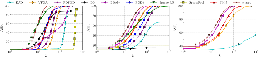
Figure 2: Robustness evaluation curves, showing the ASR against the perturbation budget $k$, for M2 on MNIST (left), C2 on CIFAR10 (middle), and I1 on ImageNet (right). The ASR is the fraction of adversarial examples for which $\|\bm{\mathbf{\delta}}^{\star}\|_{0}<k$.

Robustness Evaluation Curves. Complementary to the performance results shown in Tables I-III, we present the robustness evaluation curves in Fig. 2 for each attack on M2, C2, and I1. These curves go beyond the only median statistic and ASR_k, providing further evidence that $\mathtt{\sigma}$-zero achieves higher ASRs with smaller $\ell_{0}$-norm perturbations compared to the competing attacks. Moreover, the ASR of our attack reaches almost always $100\%$ as the perturbation budget grows, meaning that its optimization only fails rarely, and thus providing more reliable adversarial robustness evaluations (Carlini et al., 2019; Pintor et al., 2022). These results reinforce our previous findings that $\mathtt{\sigma}$-zero is an efficient and effective method for generating adversarial examples with a smaller $\ell_{0}$ norm. In Appendix C-C, we include similar curves for all other experimental configurations, for which results are consistent. In summary, $\mathtt{\sigma}$-zero consistently outperforms other state-of-the-art methods, suggesting that it can find smaller and more effective perturbations, making it a highly promising robustness evaluation method.

Comparison with Fixed-budget Attacks. We conclude our experiments by evaluating $\mathtt{\sigma}$-zero against PGD-$\ell_{0}$ and Sparse-RS, which search for perturbations within a fixed budget $k$. In these evaluations, we consider $N=1000$ for $\mathtt{\sigma}$-zero and PGD-$\ell_{0}$, while we set $N=2000$ for Sparse-RS. Both PGD-$\ell_{0}$ and Sparse-RS use all the iterations to optimize the attack for each given $k$ value, while $\mathtt{\sigma}$-zero is just run once to find the minimum-norm adversarial examples. Note indeed that this setting is unfair to $\mathtt{\sigma}$-zero, as our attack aims to solve a more challenging optimization problem using much fewer iterations. In particular, we run PGD-$\ell_{0}$ and Sparse-RS with $k=24,50,100$ on MNIST and CIFAR10, while we only run Sparse-RS with $k=150$ on ImageNet (discarding PGD-$\ell_{0}$, which turned out to be too computationally-demanding), as suggested by Croce et al. (2022). The results are reported in Tables VIII-IX in Appendix C-B, where we also include the additional comparison using $10\times$ fewer steps for each attack. The results confirm once again that, despite the unfair setup considered here, $\mathtt{\sigma}$-zero still outperforms competing approaches.

IV Related Work

Due to the inherent complexity of optimizing over non-convex and non-differentiable constraints, developing gradient-based attacks to optimize $\ell_{0}$-norm adversarial examples is not trivial. We categorize them into two main groups: (i) multiple-norm attacks extended to $\ell_{0}$, and (ii) attacks specifically designed to optimize the $\ell_{0}$ norm. We also discuss related work that leverages the approximation of the $\ell_{0}$-norm used in this paper for different goals.

Multiple-norm Attacks Extended to $\ell_{0}$. These attacks are developed to work with multiple $\ell_{p}$ norms and include the extension of their algorithms to the $\ell_{0}$ norm. While they are able to find sparse perturbations, they often require a strong use of heuristics to work in this setting. Brendel et al. (2019a) initializes the attack from an adversarial example far away from the clean sample and optimizes the perturbation by walking with small steps on the decision boundary trying to get closest to the original sample. In general, the algorithm can be used for any $\ell_{p}$ norm, including $\ell_{0}$, but the individual optimization steps are very costly. Pintor et al. (2021) propose the FMN attack that does not require an initialization step and converges efficiently with lightweight gradient-descent steps. However, their approach was developed to generalize over $\ell_{p}$ norms, but does not make special adaptations to minimize the $\ell_{0}$ norm specifically. Matyasko and Chau (2021) optimize the trade-off between perturbation size and loss of the attack and uses relaxations of the $\ell_{0}$ norm (e.g., $\ell_{1/2}$) to promote sparsity. However, this scheme does not strictly minimize the $\ell_{0}$ norm, as the relaxation does not set the lowest components exactly to zero.

$\bm{\ell}_{0}$-specific Attacks. Croce et al. (2022) introduced Sparse-RS, a random search-based attack that, unlike minimum-norm attacks, aims to find adversarial examples that are misclassified with high confidence within a fixed perturbation budget. Césaire et al. (2021) have designed an attack specifically for the $\ell_{0}$ norm, modeled as a stochastic Markov problem. It induces folded Gaussian noise to selected input components, iteratively finding the set that achieves misclassification with the minimum perturbation. However, this attack requires a considerable amount of memory to explore the possible combinations and to find an optimal solution, thereby hindering its scalability. Our attack combines the benefits of both groups, i.e., effectiveness and efficiency, providing the state-of-the-art solution for adversarial robustness evaluations of DNNs when considering $\ell_{0}$-norm attacks — a relatively underexplored scenario in existing benchmarks (Croce et al., 2021).

$\ell_{0}$-norm Approximation. Given the non-convex and discontinuous nature of the $\ell_{0}$ norm, the adoption of surrogate approximation functions has been extensively studied (Bach et al., 2012; Weston et al., 2003; Zhang, 2008). Chen et al. (2018) use elastic-net regularization to calculate sparse perturbations. However, their attack is not designed to find minimum $\ell_{0}$-norm perturbations. Our work uses the formulation proposed by Osborne et al. (2000b), which provides an unbiased estimate of the actual $\ell_{0}$ norm. More recently, it has been employed by Cinà et al. (2022) in the context of poisoning attacks for increasing the energy consumption of DNNs, and by Lazzaro et al. (2023); Runwal et al. (2023) for training energy-saving DNNs. To the best of our knowledge, we are the first to use this approximation to facilitate optimization of minimum $\ell_{0}$-norm adversarial examples.

V Conclusions, Limitations, and Future Work

Despite numerous attacks have been proposed to evaluate adversarial robustness of DNNs, the significance of $\ell_{0}$-norm attacks in this context has been significantly overlooked (Chen et al., 2018; Croce and Hein, 2021a). Nevertheless, these attacks are able to identify a few input values that, if modified, can subvert the model’s predictions, revealing crucial information about the limitations of current models. We argue that this literature gap is primarily due to the non-convex and non-differentiable nature of the $\ell_{0}$ norm, which poses challenges for gradient-based optimization.

In this work, we propose $\mathtt{\sigma}$-zero, a novel attack aimed to find minimum $\ell_{0}$-norm adversarial examples, based on the following main technical contributions: (i) the use of a differentiable approximation of the $\ell_{0}$ norm to define a novel, smooth objective that can be minimized via gradient descent; and (ii) the definition of an adaptive projection operator to further increase the sparsity of the adversarial perturbation, by zeroing out the least relevant features in each iteration. Our attack also leverages specific optimization tricks to stabilize and speed up the optimization. Our extensive experiments have shown the superior effectiveness and efficiency of $\mathtt{\sigma}$-zero in diverse scenarios, specifically for finding minimal $\ell_{0}$-norm perturbations. Our approach consistently discovers minimum-norm perturbations across all models and datasets while maintaining computational efficiency and low memory consumption at runtime without requiring any computationally demanding hyperparameter tuning. By identifying the smallest number of inputs that can be modified to mislead the target model, $\mathtt{\sigma}$-zero provides valuable insights on the vulnerabilities of DNNs and what they learn as salient input characteristics. In conclusion, $\mathtt{\sigma}$-zero emerges as a highly promising candidate for establishing a standardized benchmark to evaluate robustness against sparse $\ell_{0}$ perturbations and promoting the development of novel robust models against sparse attacks.

Appendix A Robust Models

The experimental setup described in this paper (Sect. III-A) utilizes pre-trained baseline and robust models obtained from RobustBench Croce et al. (2021). The goal of RobustBench is to track the progress in adversarial robustness for $\ell_{\infty}$ and $\ell_{2}$-norm attacks since these are the most studied settings in the literature. We summarize in Table IV the models we employed for testing the performance of $\mathtt{\sigma}$-zero. Each entry in the table includes the label reference from RobustBench, the short name we assigned to the model, and the corresponding clean and robust accuracy under the specific threat model. The robustness of these models is evaluated against an ensemble of white-box and black-box attacks, specifically AutoAttack. Complementary, we also include in our experiments models trained to be robust against $\ell_{1}$ sparse attacks, i.e., (Croce and Hein, 2021b) and (Jiang et al., 2023). Our experimental setup is designed to encompass a wide range of model architectures and defensive techniques, ensuring a comprehensive and thorough performance evaluation of the considered attacks.

TABLE IV: Summary of Robustbench Croce et al. (2021) models used in our experiments. For each model, we report its reference label in Robustbench Croce et al. (2021), its threat model, and corresponding clean and robust accuracy.

Dataset	Reference	Model	Threat model	Clean accuracy %	Robust accuracy %
CIFAR10	Standard	C1 (Croce et al., 2021)	-	94.78	0
	Carmon2019Unlabeled	C2 (Carmon et al., 2019)	$\ell_{\infty}$	89.69	59.53
	Augustin2020Adversarial	C3 (Augustin et al., 2020)	$\ell_{2}$	91.08	72.91
	Engstrom2019Robustness	C4 (Engstrom et al., 2019)	$\ell_{\infty}$- $\ell_{2}$	87.03 - 90.83	49.25 - 69.24
	Gowal2020Uncovering	C6 (Gowal et al., 2021)	$\ell_{2}$	90.90	74.50
	Chen2020Adversarial	C7 (Chen et al., 2020)	$\ell_{\infty}$	86.04	51.56
	Xu2023Exploring_WRN-28-10	C8 (Xu et al., 2023)	$\ell_{\infty}$	93.69	63.89
	Addepalli2022Efficient_RN18	C9 (Addepalli et al., 2022)	$\ell_{\infty}$	85.71	52.48
Imagenet	Standard_R18	I1 (He et al., 2015)	-	76.52	0
	Engstrom2019Robustness	I2 (Engstrom et al., 2019)	$\ell_{\infty}$	62.56	29.22
	Wong2020Fast	I3 (Wong et al., 2020)	$\ell_{\infty}$	55.62	26.24
	Salman2020Do_R18	I4 (Salman et al., 2020)	$\ell_{\infty}$	64.02	34.96
	Hendrycks2020Many	I5 (Hendrycks et al., 2021)	$\ell_{\infty}$	76.86	52.90
	Debenedetti2022Light_XCiT-S12	I6 (Debenedetti et al., 2023)	$\ell_{\infty}$	72.34	41.78

Appendix B $\mathtt{\sigma}$-zero Investigation

B-A $\mathtt{\sigma}$-zero Objective Function Visualization

In Figure 3, we depict the behavior of the loss terms of $\mathtt{\sigma}$-zero when applied to the Imagenet data sample, specifically, the frog in Figure 1. When the sample is not adversarial, the attack algorithm increases the $\ell_{0}$ norm, highlighted by the bumps in the orange curve, to find a valid adversarial $\bm{\mathbf{\delta}}$. Conversely, when an adversarial example is found, the loss term is cropped to zero, and the algorithm focus solely on minimizing the $\ell_{0}$ in $\bm{\mathbf{\delta}}$.

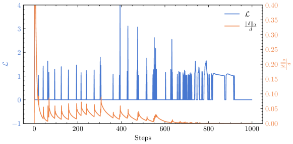
Figure 3: $\mathtt{\sigma}$-zero loss terms during the optimization procedure.

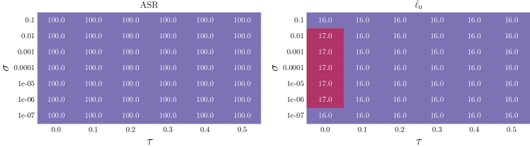
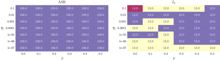
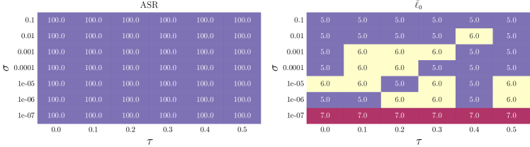
Figure 4: Ablation study on $\sigma$ (y-axis) and $\tau$ (x-axis) for MNIST M1 (top-row), CIFAR10 C9 (middle-row), IMAGENET I1, (bottom-row). For each combination, we report the attack success rate (leftmost matrix) and the mean $\ell_{0}$ norm on the output adversarial perturbation (rightmost matrix).

B-B Ablation Study

To assess the strength and potential limitations of our proposed attack, we conducted an ablation study on its key hyperparameters. Specifically, we investigated the impact of varying two critical parameters, $\tau_{0}$ and $\sigma$. The parameter $\tau_{0}$ governs the initial tolerance threshold in Algorithm 1, which induces sparsity within the adversarial noise. Conversely, $\sigma$ defines the approximation quality of $\hat{\ell}_{0}$ in Equation 7 compared to the actual $\ell_{0}$ function. Our ablation study, depicted in Figure 4, involved three distinct models: M1 (top row), C9 (middle row) and I1 (bottom row). We executed the attack on 1000 randomly selected samples from each dataset and recorded the ASR_∞ and the median $\ell_{0}$ norm of the resulting adversarial perturbations. Remarkably, we observe a significant robustness of $\mathtt{\sigma}$-zero with respect to these two hyperparameters, except for the extreme case of $\sigma=1$. With regard to the $\tau_{0}$ parameter, it is observed that the choice of the initial value exerts negligible influence on the ultimate outcome, given that the parameter dynamically adapts throughout the optimization process. Concerning $\sigma$, as also noted in Cinà et al. (2022), its selection is not particularly challenging, especially when incorporating the sparsity projection operator. Overall, the ablation study revealed consistent trends across the models. In all cases, we identified a broad parameter configuration range where our attack maintained robustness, making hyperparameter optimization for the attacker a swift task. This robustness is further evidenced by the results presented in both Tables I-III and Tables V-VII, where our attack consistently outperforms state-of-the-art attacks even with a shared hyperparameter configuration across all models.

Appendix C Additional Experimental Comparisons

C-A Attack Comparison with 100 steps

In our experimental setup, we also explore scenarios where the attacker’s access to queries is limited, thus reducing the number of iterations for the attack. To simulate this perspective, we replicate our experimental comparison involving $\mathtt{\sigma}$-zero and state-of-the-art sparse attacks while restricting the number of steps to $100$. The results are summarized in Tables V-VII. Notably, compared to the results presented in Tables I-III, considering 1000 steps, most competitive attacks undergo a decrease in their ASRs, while $\mathtt{\sigma}$-zero consistently maintains a 100% success rate. In conclusion, $\mathtt{\sigma}$-zero remains a promising choice for crafting minimum $\ell_{0}$-norm attacks against DNNs, even when the attacker has limited query resources.

TABLE V: Results on MNIST with $N=100$. For each attack and model (M), we report ASR at $k=10,50,\infty$, median perturbation size $\tilde{\ell}_{0}$, mean runtime $t$ (in seconds), mean number of queries $q$ ($\div$ 1000), and maximum VRAM usage (in GB).

Attack	M	ASR10	ASR50	ASR∞	$\mathbf{\tilde{\ell}}_{0}$	$\mathbf{t}$	$\mathbf{q}$	VRAM	M	ASR10	ASR50	ASR∞	$\tilde{\ell}_{0}$	$\mathbf{t}$	$\mathbf{q}$	VRAM
EAD		1.11	46.65	100.0	52	0.06	1.14	0.07		1.2	35.57	100.0	61	0.06	0.99	0.07
VFGA		9.62	82.68	100.0	27	0.07	0.76	0.23		1.82	38.99	99,98	57	0.07	1.34	0.24
PDPGD		0.98	0.98	100.0	359	0.01	0.20	0.07		0.52	0.52	95.02	254	0.01	0.2	0.07
BB		12.80	98.00	100.0	20	0.13	1.19	0.08		26.53	83	87.87	18	0.13	1.69	0.08
BBadv		12.32	90.88	100.0	21	0.09	0.21	0.08		17.52	58.8	100.0	34	0.07	0.21	0.08
PGD-$\ell_{0}$		10.64	96.93	100.0	24	0.04	0.20	0.07		2.32	71.98	97.2	37	0.16	0.2	0.07
Sparse-RS		2.17	9.67	61.88	146	0.24	0.26	0.07		3.68	31.16	56.03	107	0.24	0.24	0.08
SPARSEFOOL		4.86	6.76	96.98	469	1.07	0.18	0.07		0.93	1.21	91.68	463	2.87	0.86	0.07
FMN		7.22	83.09	88.92	30	0.01	0.20	0.07		4.02	14.03	14.81	$\bm{{\color[rgb]{1,0,0}\infty}}$	0.01	0.2	0.07
1-17 $\mathtt{\sigma}$-zero	M1	12.14	98.45	100.0	22	0.01	0.20	0.08	M2	36.49	99.82	100.0	13	0.01	0.2	0.8

TABLE VI: Attack results for CIFAR10 with 100 steps. The symbol ^∗ in VFGA suggests a potential overestimation due to using a smaller batch size for memory constraints. See the caption of Table VI for further details.

Attack	M	ASR10	ASR50	ASR∞	$\mathbf{\tilde{\ell}}_{0}$	$\mathbf{t}$	$\mathbf{q}$	VRAM	M	ASR10	ASR50	ASR∞	$\mathbf{\tilde{\ell}}_{0}$	$\mathbf{t}$	$\mathbf{q}$	VRAM
EAD		6.82	19.09	100.0	146	0.26	0.77	1.58		14.35	32.94	100.0	83	1.58	0.82	10.04
VFGA		49.14	93.44	98.99	11	0.17	0.38	12.08		27.63	67.05	87.75	29	3.75	0.86	> 40
PDPGD		5.23	5.23	100.0	3057	0.05	0.20	1.43		11.26	11.26	99.75	2814	0.32	0.2	8.97
BB		53.48	97.55	100.0	10	0.62	0.95	1.59		13.18	16,88	17.91	$\bm{{\color[rgb]{1,0,0}\infty}}$	2.67	1.95	10.04
BBadv		52.08	97.35	100.0	10	0.45	0.21	1.59		34.98	84.59	100.0	18	0.76	0.21	10.04
PGD-$\ell_{0}$		26.69	73.61	100.0	24	0.51	0.19	1.74		20.3	45.95	100.0	57	1.8	0.19	10.95
Sparse-RS		33.66	82.88	100.0	19	0.63	0.27	1.70		20.64	39.06	93.43	96	2.15	0.3	10.92
SparseFool		11.19	11.19	56.56	3072	1.42	0.37	1.56		16.74	16.79	35.36	$\bm{{\color[rgb]{1,0,0}\infty}}$	19.74	0.62	10.00
FMN		62.85	97.72	98.86	8	0.05	0.20	1.43		27.16	61.49	72.34	33	0.31	0.2	8.98
1-17 $\mathtt{\sigma}$-zero	C1	57.54	99.84	100.0	9	0.08	0.20	1.83	C6	37.82	87.2	100.0	16	0.44	0.2	10.29
EAD		12.74	28.74	100.0	100.0	0.27	0.80	1.53		16.95	29.59	100.0	128	0.67	0.66	5.51
VFGA		28.98	75.34	93.69	24	0.23	0.72	11.83		34.27	82.04	97.08	20	4.32	0.61	> 40
PDPGD		10.31	10.31	99.39	2421	0.05	0.20	1.43		13.96	13,96	54,16	3072	0.21	0.2	5.23
BB		11.58	14.29	14.97	$\bm{{\color[rgb]{1,0,0}\infty}}$	0.44	1.95	1.59		25.89	78.14	84.46	17	1.36	1.67	5.55
BBadv		33.01	86.63	100.0	18	0.41	0.21	1.59		40.92	91.58	100.0	14	0.55	0.21	5.51
PGD-$\ell_{0}$		30.57	48.43	100.0	54	0.20	0.19	1.72		26.0	58.57	100.0	36	2.42	0.19	6.41
Sparse-RS		17.62	33.21	92.51	127	0.76	0.31	1.71		18.75	28.45	76.9	237	2.71	0.26	6.40
SparseFool		17.47	17.76	47.26	$\bm{{\color[rgb]{1,0,0}\infty}}$	3.17	0.35	1.62		23.67	24.85	62.42	3072	9.86	0.2	5.50
FMN		28.06	69.36	80.68	27	0.05	0.20	1.43		32.98	76.59	87.1	22.0	0.21	0.2	5.24
1-17 $\mathtt{\sigma}$-zero	C2	36.41	88.27	100.0	16	0.08	0.20	1.84	C7	41.07	91.87	100.0	14	0.25	0.2	6.76
EAD		9.14	10.67	100.0	451	0.30	0.71	2.01		9.23	21.61	100.0	162	0.31	0.8	2.27
VFGA		21.69	66.46	91.64	33	0.34	0.87	16.64		22.75	56.56	75.79	39.5	1.45	1.06	> 40
PDPGD		8.92	8.92	75.31	3052	0.09	0.20	1.91		6.31	6.31	96.2	2773	0.06	0.2	2.11
BB		19.46	53.53	57.05	40	0.59	1.90	2.00		35.42	90.74	100.0	16	0.65	1.07	2.27
BBadv		29.14	92.74	100.0	19	0.40	0.21	2.00		34.2	89.7	100.0	17	0.42	0.21	2.27
PGD-$\ell_{0}$		16.51	46.08	100.0	54	0.31	0.19	2.30		15.78	45.03	100.0	57	0.7	0.2	2.59
Sparse-RS		12.68	21.20	70.59	234	1.03	0.25	2.30		13.43	32.25	99.43	117	0.86	0.31	2.57
SparseFool		14.26	20.59	94.26	3071	2.44	0.26	1.91		11.98	12.14	70.77	3072	3.28	0.22	2.25
FMN		20.37	62.41	71.3	36	0.08	0.20	1.92		23.21	59.69	68.88	35	0.06	0.2	2.19
1-17 $\mathtt{\sigma}$-zero	C3	27.07	88.60	100.0	21	0.11	0.20	2.25	C8	36.15	90.95	100.0	16	0.09	0.2	2.52
EAD		9.38	10.56	100.0	434	0.48	0.90	2.00		15.76	26.17	100.0	144	0.11	0.79	0.52
VFGA		30.44	90.04	99.16	19	0.29	0.52	16.64		29.56	74.14	94.16	26	0.12	0.73	3.18
PDPGD		9.17	9.17	99.90	2709	0.12	0.20	1.91		14.29	14.29	90.95	3057	0.03	0.2	0.47
BB		16.28	32.41	32.83	$\bm{{\color[rgb]{1,0,0}\infty}}$	0.50	1.93	2.00		35.98	89.39	100.0	17	0.43	1.13	0.53
BBadv		35.44	98.37	100.0	15	0.41	0.21	2.00		35.36	90.08	100.0	17	0.35	0.21	0.53
PGD-$\ell_{0}$		19.54	60.78	100.0	36	0.25	0.19	2.30		23.77	51.18	100.0	48	0.14	0.19	0.56
Sparse-RS		12.57	20.21	67.12	262	0.99	0.25	2.30		18.14	25.98	70.20	301	0.46	0.25	0.54
SparseFool		15.48	38.76	82.71	3062	4.30	9.67	1.90		23.18	26.54	51.90	3072	0.58	0.33	0.52
FMN		26.63	79.48	87.20	24	0.08	0.20	1.91		29.47	69.77	80.68	27	0.03	0.2	0.48
1-17 $\mathtt{\sigma}$-zero	C4	33.65	94.90	100.0	16	0.11	0.20	2.25	C9	35.47	86.02	100.0	18	0.04	0.2	0.77
EAD		12.95	13.18	100.0	835	0.11	0.65	0.64		23.87	24.4	100.0	844	0.12	0.66	0.65
VFGA		18.94	49.73	82.94	51	0.13	1.13	4.44		33.58	69.52	93.05	28	0.14	0.77	4.22
PDPGD		12.95	12.98	99.47	2566	0.04	0.20	0.59		23.78	23.78	66.62	3072	0.04	0.2	0.59
BB		14.13	22.91	27.64	$\bm{{\color[rgb]{1,0,0}\infty}}$	1.04	2.25	0.65		24.72	27.98	29.51	$\bm{{\color[rgb]{1,0,0}\infty}}$	0.54	2.09	0.65
BBadv		19.17	66.79	100.0	37	0.40	0.21	0.65		35.36	80.64	100.0	23	0.36	0.21	0.65
PGD-$\ell_{0}$		16.65	32.12	100.0	84	0.48	0.19	0.71		28.22	43.44	100.0	63	0.43	0.19	0.71
Sparse-RS		14.40	17.91	87.58	378	0.50	0.28	0.69		26.65	32.35	75.74	211	0.55	0.23	0.69
SparseFool		15.89	24.36	58.29	3072	1.63	0.48	0.66		26.85	42.97	84.45	70	1.54	0.47	0.66
FMN		18.55	37.90	43.90	$\bm{{\color[rgb]{1,0,0}\infty}}$	0.03	0.20	0.59		32.63	58.78	65.83	35	0.03	0.2	0.59
1-17 $\mathtt{\sigma}$-zero	C5	19.19	57.71	100.0	43	0.04	0.20	0.89	C10	34.61	73.75	100.0	25	0.04	0.2	0.89

TABLE VII: Attack results for Imagenet with 100 steps. The symbol ^∗ in VFGA suggests a potential overestimation due to using a smaller batch size for memory constraints. See the caption of Table VI for further details.

Attack	M	ASR10	ASR50	ASR∞	$\mathbf{\tilde{\ell}}_{0}$	$\mathbf{t}$	$\mathbf{q}$	VRAM	M	ASR10	ASR50	ASR∞	$\mathbf{\tilde{\ell}}_{0}$	$\mathbf{t}$	$\mathbf{q}$	VRAM
EAD		34.2	35.9	100.0	484	1.02	0.67	0.46		55.5	60.0	100.0	0	1.03	0.72	0.48
VFGA		47.0	72.2	85.3	14	1.06	0.70	> 40		61.8	75.2	83.9	0	0.91	0.59	> 40
BBadv		50.6	83.3	100.0	10	23.02	0.21	0.72		70.1	89.1	100.0	0	19.68	0.21	0.73
FMN		47.4	64.5	68.1	14	0.08	0.20	0.66		63.0	74.9	77.2	0	0.07	0.2	0.67
1-17 $\mathtt{\sigma}$-zero	I1	51.2	86.9	100.0	10	0.13	0.20	0.84	I4	71.9	90.5	100.0	0	0.12	0.2	0.84
EAD		44.8	50.1	100.0	48	2.32	0.68	1.42		26.6	27.7	100.0	1108	0.58	0.61	1.41
VFGA		49.0	63.2	96.7	13	2.88	0.72	> 40		36.4	58.7	74.0	31	3.07	0.96	> 40
BBadv		57.8	80.1	100.0	5	20.49	0.21	2.40		40.7	74.7	100.0	20	23.86	0.21	2.41
FMN		50.6	60.0	62.4	10	0.20	0.20	2.30		36.3	50.6	53.2	47	0.16	0.2	2.30
1-17 $\mathtt{\sigma}$-zero	I2	58.0	82.7	100.0	4	0.29	0.20	2.52	I5	39.5	74.4	100.0	21	0.23	0.2	2.52
EAD		54.5	60.2	100.0	0	2.46	0.72	1.41		32.2	33.0	100.0	808	5.15	0.7	1.68
VFGA		62.2	76.0	83.0	0	2.33	0.59	> 40		35.4	46.8	56.9	66.5	9.23	1.2	> 40
BBadv		70.1	87.8	100.0	0	18.60	0.21	2.41		37.8	58.0	99.9	32	21.23	0.21	3.07
FMN		64.2	72.0	74.3	0	0.20	0.20	2.30		35.7	46.2	47.5	$\bm{{\color[rgb]{1,0,0}\infty}}$	0.44	0.2	2.97
1-17 $\mathtt{\sigma}$-zero	I3	69.9	89.3	100.0	0	0.29	0.20	2.52	I6	38.1	55.2	100.0	39	0.61	0.2	3.20

C-B Comparison with Fixed-budget Attacks

In our experimental comparisons presented in both Tables I-III and Tables V-VII, we include the Sparse-RS and PGD-$\ell_{0}$ attacks introduced by (Croce et al., 2022) and (Croce and Hein, 2019). These attacks have been designed to generate sparse adversarial perturbations given a fixed budget $k$, therefore, drawing comparisons with minimum-norm attacks is not a straightforward task. Specifically, in their threat model, the attacker imposes a maximum limit on the number of perturbed features, and the attack then outputs the adversarial example that minimizes the model’s confidence in predicting the true label of the sample. However, since the fixed-budget threat model differs from the minimum-norm scenario we consider in this paper, which do not assume a maximum budget, we have developed a wrapper around Sparse-RS and PGD-$\ell_{0}$ to ensure a fair comparison. Similarly to (Rony et al., 2021b), we employ a sample-wise binary search strategy to determine the smallest budget, denoted as $k$, that must be provided as input to them to achieve an ASR equal to $100\%$ on the data. At each iteration of the binary search, if the attack is successful, we halve the value of $k$, asking Sparse-RS and PGD-$\ell_{0}$ to perturb fewer features. Conversely, if the sample is not adversarial, we double the value of $k$. Thus, we enable the attacker to find the value of $k$ that results in the minimum $\ell_{0}$ norm for each sample. Finally, the comparison tables showcase the best result with the minimum norm perturbation in the median across the iterations. We also provide further evaluation of $\mathtt{\sigma}$-zero in a fixed-budget approach in Tables VIII-XI. Tables VIII and X include different experiments on MNIST and CIFAR10, fixing diverse feature budgets and maximum iterations. In Table XI, experiments on ImageNet are evaluated in a low query scenario. The results once again affirm that, despite the unfair setup considered here, $\mathtt{\sigma}$-zero consistently outperforms competing approaches.

TABLE VIII: Fixed budget comparison results with 1000 steps on MNIST and CIFAR10. For each attack, we report the corresponding ASR with different feature budget levels (24,50,100).

Attack	M	ASR24	ASR50	ASR100	$\mathbf{t}$	$\mathbf{q}$	VRAM	M	ASR24	ASR50	ASR100	$\mathbf{t}$	$\mathbf{q}$	VRAM
MNIST
PGD-$\ell_{0}$		73.99	99.90	100.0	0.26	2.0	0.07		61.87	94.15	98.50	0.26	2.0	0.07
Sparse-RS		79.54	96.35	99.79	0.67	0.83	0.06		98.92	99.96	100.0	0.20	0.24	0.06
1-15$\mathtt{\sigma}$-zero	M1	83.79	99.98	100.0	0.31	2.00	0.04	M2	98.03	100.0	100.0	0.31	2.00	0.04
CIFAR10
PGD-$\ell_{0}$		68.60	88.89	98.14	1.16	2.0	1.44		32.80	50.53	77.06	4.8	2.0	9.00
Sparse-RS		99.71	100.0	100.0	0.16	0.08	1.41		76.61	89.88	96.22	1.64	0.67	8.96
1-15$\mathtt{\sigma}$-zero	C1	99.20	100.0	100.0	0.74	2.00	1.51	C6	75.63	94.47	99.78	4.41	2.00	10.43
PGD-$\ell_{0}$		38.18	59.67	87.19	1.31	2.0	1.44		42.81	66.19	90.49	4.06	2.0	5.23
Sparse-RS		72.51	86.59	94.28	0.81	0.77	1.42		72.54	86.72	94.84	2.19	0.78	5.22
1-15$\mathtt{\sigma}$-zero	C2	76.53	95.38	99.94	0.73	2.00	1.53	C7	81.23	97.33	99.97	2.75	2.00	5.90
PGD-$\ell_{0}$		32.41	59.19	89.22	1.79	2.0	1.91		31.45	52.79	80.27	1.32	2.0	2.13
Sparse-RS		59.24	79.81	92.43	1.25	1.04	1.90		68.77	82.06	89.81	0.88	0.85	2.10
1-15$\mathtt{\sigma}$-zero	C3	74.63	97.55	99.99	1.41	2.00	1.92	C8	79.59	96.93	99.91	0.89	2.00	2.65
PGD-$\ell_{0}$		37.91	68.90	95.31	1.77	2.0	1.91		38.33	61.88	89.50	0.99	2.0	0.49
Sparse-RS		63.75	84.49	95.74	1.21	0.97	1.90		64.80	81.46	91.13	0.81	0.91	0.47
1-15$\mathtt{\sigma}$-zero	C4	81.38	99.15	100.0	1.39	2.00	1.91	C9	73.96	94.21	99.80	0.63	2.00	0.51
PGD-$\ell_{0}$		22.99	36.20	67.54	1.00	2.0	0.6		34.35	44.99	68.61	1.02	2.0	0.6
Sparse-RS		30.87	45.65	63.26	1.17	1.47	0.59		49.35	63.01	76.51	0.94	1.11	0.59
1-15$\mathtt{\sigma}$-zero	C5	38.60	73.02	98.58	0.43	2.00	0.71	C10	55.42	82.92	99.19	0.42	2.00	0.72

TABLE IX: Fixed budget comparison results with 1000 steps on ImageNet. For each attack, we report the corresponding ASR with feature budget level equal to 150.

Attack	M	ASR150	$\mathbf{t}$	$\mathbf{q}$	VRAM	M	ASR150	$\mathbf{t}$	$\mathbf{q}$	VRAM
Sparse-RS		91.5	1.71	0.34	1.33		89.2	6.81	0.32	1.33
$\mathtt{\sigma}$-zero	I1	100.0	1.18	2.00	0.84	I4	98.8	1.13	2.00	0.84
Sparse-RS		84.1	9.19	0.49	3.47		72.2	8.04	0.77	3.48
$\mathtt{\sigma}$-zero	I2	97.0	2.75	2.00	2.52	I5	99.3	2.76	2.00	2.52
Sparse-RS		87.5	9.56	0.35	3.47		47.4	11.88	1.15	4.30
$\mathtt{\sigma}$-zero	I3	98.2	2.76	2.00	2.52	I6	86.2	5.72	2.00	3.20

TABLE X: Fixed budget comparison with 100 steps on MNIST and CIFAR10. For each attack, we report the corresponding ASR with different feature budget levels (24,50,100).

Attack	M	ASR24	ASR50	ASR100	$\mathbf{t}$	$\mathbf{q}$	VRAM	M	ASR24	ASR50	ASR100	$\mathbf{t}$	$\mathbf{q}$	VRAM
MNIST
PGD-$\ell_{0}$		70.92	99.48	100.0	0.02	0.2	0.07		51.84	89.21	96.17	0.03	0.2	0.07
Sparse-RS		27.99	50.53	83.21	0.13	0.189	0.06		70.99	86.95	97.29	0.09	0.12	0.06
1-15$\mathtt{\sigma}$-zero	M1	61.12	98.45	100.0	0.01	0.20	0.08	M2	98.03	100.0	100.0	0.01	0.2	0.8
CIFAR10
PGD-$\ell_{0}$		64.32	84.12	96.02	0.12	0.2	1.33		32.47	49.64	75.27	0.39	0.2	9.00
Sparse-RS		92.46	98.54	99.87	0.07	0.05	1.41		50.32	64.89	77.73	0.25	0.13	8.96
1-15$\mathtt{\sigma}$-zero	C1	91.54	99.84	100.0	0.08	0.20	1.83	C6	63.44	87.2	98.17	0.44	0.2	10.29
PGD-$\ell_{0}$		35.93	55.37	83.26	0.12	0.2	1.46		42.17	64.64	88.12	0.39	0.2	5.23
Sparse-RS		43.39	58.52	71.51	0.13	0.14	1.4		42.51	57.51	70.56	0.26	0.13	5.22
1-15$\mathtt{\sigma}$-zero	C2	63.60	88.27	99.16	0.08	0.20	1.84	C7	69.49	91.87	99.58	0.25	0.2	6.76
PGD-$\ell_{0}$		31.94	57.25	86.43	0.17	0.2	1.91		31.22	51.48	77.24	0.12	0.2	2.13
Sparse-RS		33.08	48.15	65.2	0.16	0.15	1.90		39.31	55.78	71.15	0.14	0.15	2.11
1-15$\mathtt{\sigma}$-zero	C3	56.94	88.60	99.67	0.11	0.20	2.25	C8	65.96	90.95	99.53	0.09	0.2	2.52
PGD-$\ell_{0}$		38.30	67.59	94.95	0.18	0.2	1.91		38.25	58.56	85.31	0.10	0.2	0.49
Sparse-RS		33.78	50.54	69.09	0.16	0.15	1.90		37.93	50.7	63.66	0.12	0.14	0.47
1-15$\mathtt{\sigma}$-zero	C4	68.14	94.9	99.93	0.11	0.20	2.25	C9	60.79	86.02	98.37	0.04	0.2	0.77
PGD-$\ell_{0}$		22.84	36.16	66.8	0.10	0.2	0.60		34.06	44.72	68.55	0.10	0.2	0.6
Sparse-RS		21.24	27.01	35.95	0.13	1.65	0.59		38.51	46.27	56.89	0.11	0.13	0.56
1-15$\mathtt{\sigma}$-zero	C5	30.56	57.71	91.88	0.04	0.20	0.89	C10	49.74	73.75	95.95	0.04	0.2	0.89

TABLE XI: Fixed budget comparison results with 100 steps on ImageNet. For each attack, we report the corresponding ASR with feature budget level equal to 150.

Attack	M	ASR150	$\mathbf{t}$	$\mathbf{q}$	VRAM	M	ASR150	$\mathbf{t}$	$\mathbf{q}$	VRAM
Sparse-RS		75.4	0.72	0.07	1.33		76.6	0.71	0.06	1.33
$\mathtt{\sigma}$-zero	I1	99.6	0.13	0.20	0.84	I4	97.9	0.12	0.2	0.84
Sparse-RS		67.7	0.90	0.08	3.47		52.9	0.39	0.11	3.48
$\mathtt{\sigma}$-zero	I2	95.3	0.29	0.20	2.52	I5	96.7	0.23	0.2	2.52
Sparse-RS		76.6	0.81	0.06	3.46		38.1	0.67	0.13	4.30
$\mathtt{\sigma}$-zero	I3	96.7	0.29	0.20	2.52	I6	77.4	0.61	0.2	3.20

C-C Robustness Evaluation Curves

We present in Figs. 5-8 the robustness evaluation curves depicting the performance of $\ell_{0}$-attacks against all the models analyzed in our paper. These findings reinforce our experimental analysis, explicitly demonstrating that the $\mathtt{\sigma}$-zero attack consistently achieves higher values of ASR while employing smaller $\ell_{0}$-norm perturbations compared to alternative attacks.

C-D Visual Comparison

In Figures 11-13, we show adversarial examples generated with competing $\ell_{0}$-attacks, and our $\mathtt{\sigma}$-zero. First, we can see that $\ell_{0}$ adversarial perturbations are clearly visually distinguishable Carlini and Wagner (2017b); Brendel et al. (2019a); Pintor et al. (2021). Their goal, indeed, is not to be indistinguishable to the human eye – a common misconception related to adversarial examples (Biggio and Roli, 2018; Gilmer et al., 2018) – but rather to show whether and to what extent models can be fooled by just changing a few input values.
A second observation derived from Figures 11-13 is that the various attacks presented in the state of the art can identify distinct regions of vulnerability. For example, note how FMN and VFGA find similar perturbations, as they mostly target overlapping regions of interest. Conversely, EAD finds sparse perturbations scattered throughout the image but with a lower magnitude. This divergence is attributed to EAD’s reliance on an $\ell_{1}$ regularizer, which promotes sparsity, thus diminishing perturbation magnitude without necessarily reducing the number of perturbed features. Conversely, our attack does not focus on specific areas or patterns within the images but identifies diverse critical features, whose manipulation is sufficient to mislead the target models. Given the diverse solutions offered by the attacks, we argue that their combined usage may still improve adversarial robustness evaluation to sparse attacks.

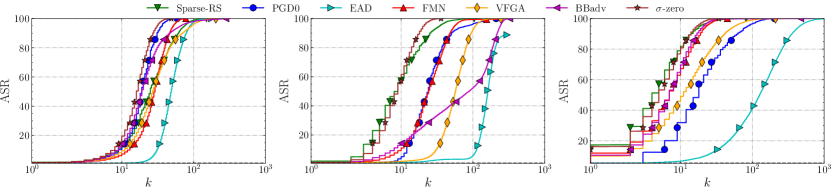
Figure 5: Robustness evaluation curves for M1 and M2 in MNIST (two leftmost plots) , C1 in CIFAR10 (rightmost plot).

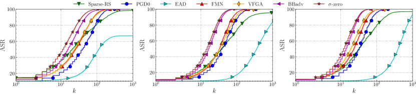
Figure 6: Robustness evaluation curves for C2, C3, and C4 in CIFAR10.

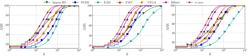
Figure 7: Robustness evaluation curves for C6, C7 and C8 in CIFAR10.

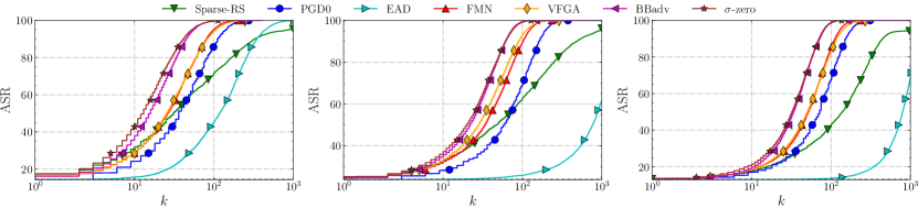
Figure 8: Robustness evaluation curves for C9, C10 and C5 in CIFAR10.

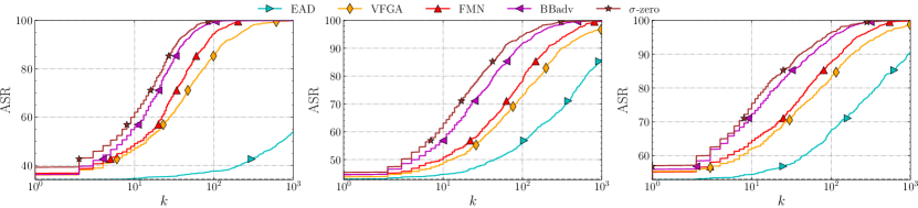
Figure 9: Robustness evaluation curves for I1, I2 and I3 in ImageNet.

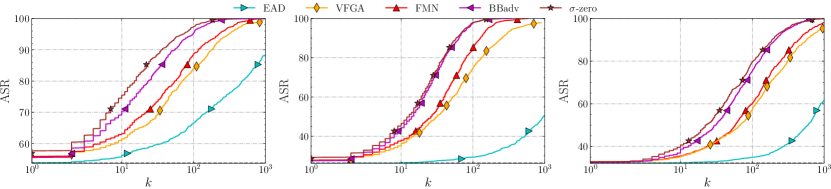
Figure 10: Robustness evaluation curves for I4, I5 and I6 in ImageNet.

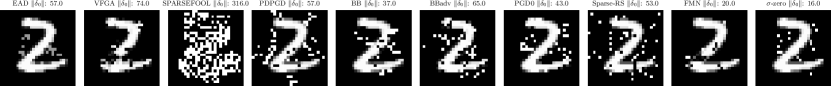
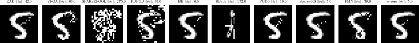
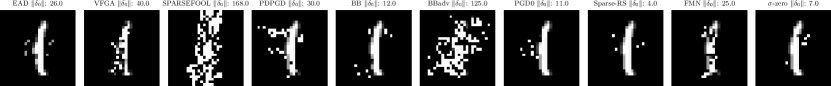
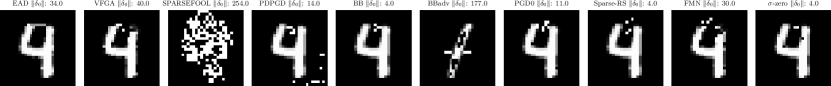
Figure 11: Randomly chosen adversarial examples from MNIST M2.

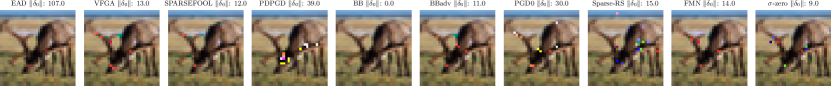
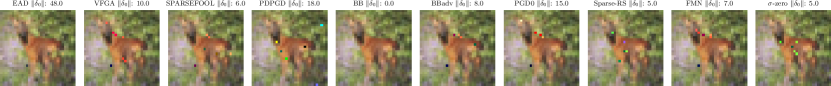
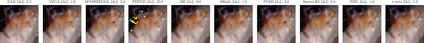
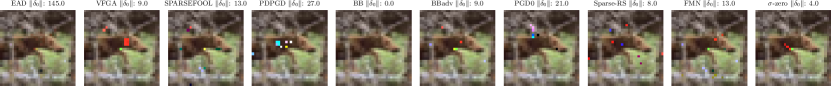
Figure 12: Randomly chosen adversarial examples from CIFAR10 C2.

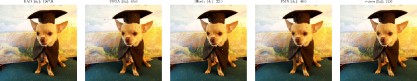
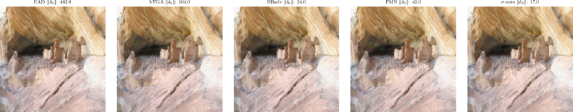
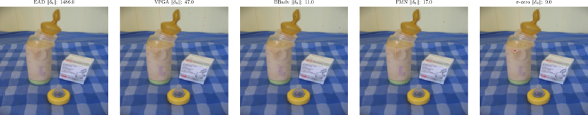
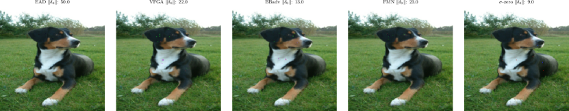
Figure 13: Randomly chosen adversarial examples from Imagenet I1.

References

- Biggio et al. (2013) B. Biggio, I. Corona, D. Maiorca, B. Nelson, N. Srndic, P. Laskov, G. Giacinto, and F. Roli, “Evasion attacks against machine learning at test time,” in Machine Learning and Knowledge Discovery in Databases - European Conference, ECML PKDD, ser. Lecture Notes in Computer Science, vol. 8190. Springer, 2013, pp. 387–402.
- Szegedy et al. (2014) C. Szegedy, W. Zaremba, I. Sutskever, J. Bruna, D. Erhan, I. Goodfellow, and R. Fergus, “Intriguing properties of neural networks,” in International Conference on Learning Representations (ICLR), 2014.
- Chen et al. (2018) P. Chen, Y. Sharma, H. Zhang, J. Yi, and C. Hsieh, “EAD: elastic-net attacks to deep neural networks via adversarial examples,” in Proceedings of the Thirty-Second AAAI Conference on Artificial Intelligence, (AAAI-18), the 30th innovative Applications of Artificial Intelligence (IAAI-18), and the 8th AAAI Symposium on Educational Advances in Artificial Intelligence (EAAI-18). AAAI Press, 2018, pp. 10–17.
- Croce and Hein (2021a) F. Croce and M. Hein, “Mind the box: l-apgd for sparse adversarial attacks on image classifiers,” in Proceedings of the 38th International Conference on Machine Learning, ICML, ser. Proceedings of Machine Learning Research, M. Meila and T. Zhang, Eds., vol. 139. PMLR, 2021, pp. 2201–2211.
- Carlini and Wagner (2017a) N. Carlini and D. A. Wagner, “Towards evaluating the robustness of neural networks,” in 2017 IEEE Symposium on Security and Privacy SP. IEEE Computer Society, 2017, pp. 39–57.
- Brendel et al. (2019a) W. Brendel, J. Rauber, M. Kümmerer, I. Ustyuzhaninov, and M. Bethge, “Accurate, reliable and fast robustness evaluation,” in Advances in Neural Information Processing Systems 32: Annual Conference on Neural Information Processing Systems, NeurIPS, 2019.
- Césaire et al. (2021) M. Césaire, L. Schott, H. Hajri, S. Lamprier, and P. Gallinari, “Stochastic sparse adversarial attacks,” in 33rd IEEE International Conference on Tools with Artificial Intelligence, ICTAI. IEEE, 2021, pp. 1247–1254.
- Matyasko and Chau (2021) A. Matyasko and L. Chau, “PDPGD: primal-dual proximal gradient descent adversarial attack,” CoRR, vol. abs/2106.01538, 2021. [Online]. Available: https://arxiv.org/abs/2106.01538
- Pintor et al. (2021) M. Pintor, F. Roli, W. Brendel, and B. Biggio, “Fast minimum-norm adversarial attacks through adaptive norm constraints,” in Advances in Neural Information Processing Systems 34: Annual Conference on Neural Information Processing Systems, NeurIPS, 2021, pp. 20 052–20 062.
- Osborne et al. (2000a) M. R. Osborne, B. Presnell, and B. A. Turlach, “On the lasso and its dual,” Journal of Computational and Graphical Statistics, vol. 9, pp. 319–337, 2000.
- Croce et al. (2021) F. Croce, M. Andriushchenko, V. Sehwag, E. Debenedetti, N. Flammarion, M. Chiang, P. Mittal, and M. Hein, “Robustbench: a standardized adversarial robustness benchmark,” in Proceedings of the Neural Information Processing Systems Track on Datasets and Benchmarks 1, NeurIPS Datasets and Benchmarks, 2021.
- Biggio and Roli (2018) B. Biggio and F. Roli, “Wild patterns: Ten years after the rise of adversarial machine learning,” Pattern Recognition, vol. 84, pp. 317–331, 2018.
- Brendel et al. (2019b) W. Brendel, J. Rauber, M. Kümmerer, I. Ustyuzhaninov, and M. Bethge, “Accurate, reliable and fast robustness evaluation,” in Conference on Neural Information Processing Systems (NeurIPS)), 2019.
- Rony et al. (2018) J. Rony, L. G. Hafemann, L. Oliveira, I. B. Ayed, R. Sabourin, and E. Granger, “Decoupling direction and norm for efficient gradient-based l2 adversarial attacks and defenses,” 2019 IEEE/CVF Conference on Computer Vision and Pattern Recognition (CVPR), pp. 4317–4325, 2018.
- LeCun and Cortes (2005) Y. LeCun and C. Cortes, “The mnist database of handwritten digits,” 2005.
- Krizhevsky (2009) A. Krizhevsky, “Learning multiple layers of features from tiny images,” 2009.
- Krizhevsky et al. (2012) A. Krizhevsky, I. Sutskever, and G. E. Hinton, “Imagenet classification with deep convolutional neural networks,” Communications of the ACM, vol. 60, pp. 84 – 90, 2012.
- Rony et al. (2021a) J. Rony, E. Granger, M. Pedersoli, and I. B. Ayed, “Augmented lagrangian adversarial attacks,” in 2021 IEEE/CVF International Conference on Computer Vision, ICCV. IEEE, 2021, pp. 7718–7727.
- Carmon et al. (2019) Y. Carmon, A. Raghunathan, L. Schmidt, J. C. Duchi, and P. S. Liang, “Unlabeled data improves adversarial robustness,” in Conference on Neural Information Processing Systems (NeurIPS)), 2019.
- Augustin et al. (2020) M. Augustin, A. Meinke, and M. Hein, “Adversarial robustness on in- and out-distribution improves explainability,” in Computer Vision - ECCV 2020 - 16th European Conference, ser. Lecture Notes in Computer Science, vol. 12371. Springer, 2020, pp. 228–245.
- Engstrom et al. (2019) L. Engstrom, A. Ilyas, H. Salman, S. Santurkar, and D. Tsipras, “Robustness (python library),” 2019. [Online]. Available: https://github.com/MadryLab/robustness
- Gowal et al. (2021) S. Gowal, S. Rebuffi, O. Wiles, F. Stimberg, D. A. Calian, and T. A. Mann, “Improving robustness using generated data,” in Advances in Neural Information Processing Systems 34: Annual Conference on Neural Information Processing Systems 2021, NeurIPS, 2021, pp. 4218–4233.
- Chen et al. (2020) T. Chen, S. Liu, S. Chang, Y. Cheng, L. Amini, and Z. Wang, “Adversarial robustness: From self-supervised pre-training to fine-tuning,” in IEEE/CVF Conference on Computer Vision and Pattern Recognition, CVPR. Computer Vision Foundation / IEEE, 2020, pp. 696–705.
- Xu et al. (2023) Y. Xu, Y. Sun, M. Goldblum, T. Goldstein, and F. Huang, “Exploring and exploiting decision boundary dynamics for adversarial robustness,” in International Conference on Learning Representations (ICLR), 2023.
- Addepalli et al. (2022) S. Addepalli, S. Jain, and V. B. R., “Efficient and effective augmentation strategy for adversarial training,” in NeurIPS, 2022.
- Croce and Hein (2021b) F. Croce and M. Hein, “Mind the box: -apgd for sparse adversarial attacks on image classifiers,” in International Conference on Machine Learning (ICML), 2021.
- Jiang et al. (2023) Y. Jiang, C. Liu, Z. Huang, M. Salzmann, and S. Süsstrunk, “Towards stable and efficient adversarial training against l1 bounded adversarial attacks,” in International Conference on Machine Learning, 2023.
- He et al. (2015) K. He, X. Zhang, S. Ren, and J. Sun, “Deep residual learning for image recognition,” 2016 IEEE Conference on Computer Vision and Pattern Recognition (CVPR), pp. 770–778, 2015.
- Wong et al. (2020) E. Wong, L. Rice, and J. Z. Kolter, “Fast is better than free: Revisiting adversarial training,” in 8th International Conference on Learning Representations, ICLR. OpenReview.net, 2020.
- Salman et al. (2020) H. Salman, A. Ilyas, L. Engstrom, A. Kapoor, and A. Madry, “Do adversarially robust imagenet models transfer better?” in Advances in Neural Information Processing Systems 33: Annual Conference on Neural Information Processing Systems 2020, NeurIPS, 2020.
- Hendrycks et al. (2021) D. Hendrycks, S. Basart, N. Mu, S. Kadavath, F. Wang, E. Dorundo, R. Desai, T. Zhu, S. Parajuli, M. Guo, D. Song, J. Steinhardt, and J. Gilmer, “The many faces of robustness: A critical analysis of out-of-distribution generalization,” in 2021 IEEE/CVF International Conference on Computer Vision, ICCV. IEEE, 2021, pp. 8320–8329.
- Modas et al. (2019) A. Modas, S.-M. Moosavi-Dezfooli, and P. Frossard, “Sparsefool: a few pixels make a big difference,” in Conference on computer vision and pattern recognition (CVPR), 2019.
- Croce and Hein (2019) F. Croce and M. Hein, “Sparse and imperceivable adversarial attacks,” 2019 IEEE/CVF International Conference on Computer Vision (ICCV), pp. 4723–4731, 2019.
- Croce et al. (2022) F. Croce, M. Andriushchenko, N. D. Singh, N. Flammarion, and M. Hein, “Sparse-rs: A versatile framework for query-efficient sparse black-box adversarial attacks,” in Thirty-Sixth AAAI Conference on Artificial Intelligence, AAAI. AAAI Press, 2022, pp. 6437–6445.
- Rony et al. (2021b) J. Rony, E. Granger, M. Pedersoli, and I. Ben Ayed, “Augmented lagrangian adversarial attacks,” in Conference on computer vision and pattern recognition (CVPR), 2021.
- (36) J. Rony and I. Ben Ayed, “Adversarial Library.” [Online]. Available: https://github.com/jeromerony/adversarial-library
- Rauber et al. (2017) J. Rauber, W. Brendel, and M. Bethge, “Foolbox: A python toolbox to benchmark the robustness of machine learning models,” 2017. [Online]. Available: https://github.com/bethgelab/foolbox
- Pintor et al. (2022) M. Pintor, L. Demetrio, A. Sotgiu, A. Demontis, N. Carlini, B. Biggio, and F. Roli, “Indicators of attack failure: Debugging and improving optimization of adversarial examples,” in Advances in Neural Information Processing Systems, S. Koyejo, S. Mohamed, A. Agarwal, D. Belgrave, K. Cho, and A. Oh, Eds., vol. 35. Curran Associates, Inc., 2022, pp. 23 063–23 076.
- Carlini et al. (2019) N. Carlini, A. Athalye, N. Papernot, W. Brendel, J. Rauber, D. Tsipras, I. J. Goodfellow, A. Madry, and A. Kurakin, “On evaluating adversarial robustness,” CoRR, vol. abs/1902.06705, 2019.
- Bach et al. (2012) F. R. Bach, R. Jenatton, J. Mairal, and G. Obozinski, “Optimization with sparsity-inducing penalties,” Found. Trends Mach. Learn., vol. 4, no. 1, pp. 1–106, 2012.
- Weston et al. (2003) J. Weston, A. Elisseeff, B. Schölkopf, and M. E. Tipping, “Use of the zero-norm with linear models and kernel methods,” J. Mach. Learn. Res., vol. 3, pp. 1439–1461, 2003.
- Zhang (2008) T. Zhang, “Multi-stage convex relaxation for learning with sparse regularization,” in NIPS, 2008.
- Osborne et al. (2000b) M. R. Osborne, B. Presnell, and B. A. Turlach, “On the lasso and its dual,” Journal of Computational and Graphical Statistics, vol. 9, pp. 319 – 337, 2000.
- Cinà et al. (2022) A. E. Cinà, A. Demontis, B. Biggio, F. Roli, and M. Pelillo, “Energy-latency attacks via sponge poisoning,” CoRR, vol. abs/2203.08147, 2022.
- Lazzaro et al. (2023) D. Lazzaro, A. E. Cinà, M. Pintor, A. Demontis, B. Biggio, F. Roli, and M. Pelillo, “Minimizing energy consumption of deep learning models by energy-aware training,” in International Conference on Image Analysis and Processing. Springer, 2023, pp. 515–526.
- Runwal et al. (2023) B. Runwal, T. Pedapati, and P.-Y. Chen, “Parameter efficient finetuning for reducing activation density in transformers,” in Annual Conference on Neural Information Processing Systems, 2023.
- Debenedetti et al. (2023) E. Debenedetti, V. Sehwag, and P. Mittal, “A light recipe to train robust vision transformers,” in First IEEE Conference on Secure and Trustworthy Machine Learning, 2023. [Online]. Available: https://openreview.net/forum?id=IztT98ky0cKs
- Carlini and Wagner (2017b) N. Carlini and D. Wagner, “Towards evaluating the robustness of neural networks,” in IEEE Symposium on Security and Privacy (S&P), 2017.
- Gilmer et al. (2018) J. Gilmer, R. P. Adams, I. J. Goodfellow, D. Andersen, and G. E. Dahl, “Motivating the rules of the game for adversarial example research,” CoRR, vol. abs/1807.06732, 2018.