Sets are all you need: Ultrafast jet classification on FPGAs for HL-LHC

Abstract

We study various machine learning based algorithms for performing accurate jet flavor classification on field-programmable gate arrays and demonstrate how latency and resource consumption scale with the input size and choice of algorithm. These architectures provide an initial design for models that could be used for tagging at the CERN LHC during its high-luminosity phase. The high-luminosity upgrade will lead to a five-fold increase in its instantaneous luminosity for proton-proton collisions and, in turn, higher data volume and complexity, such as the availability of jet constituents. Through quantization-aware training and efficient hardware implementations, we show that $\mathcal{O}(100)\text{\,ns}$ inference of complex architectures such as deep sets and interaction networks is feasible at a low computational resource cost.

1 Introduction

At the CERN Large Hadron Collider (LHC), proton beams collide every 25 ns in each of the four particle detectors located around the LHC ring. The collision events generate sprays of outgoing particles that are detected by sensors, which amount to a data rate of tens of terabytes per second. For the ATLAS [1] and CMS [2] general-purpose experiments, the data throughput is too large to record every single event. Therefore, a subset of events are selected by a real-time event filtering system, called the trigger.

The trigger system consists of two stages. First, the level-1 trigger (L1T) reduces the event rate from $\mathcal{O}(10)$ MHz to $\mathcal{O}(100)$ kHz, rejecting $\sim$99.7% of the collision events. The frequency of collisions and limited buffer size set the maximum L1T latency to $\mathcal{O}(1)\,\mu$s. Thus, the L1T is hardware based, with its algorithms running on field-programmable gate arrays (FPGAs). The second stage is represented by the high-level trigger (HLT). The HLT consists of software executed on a dedicated CPU farm and further reduces the event rate to 1 kHz. Only data accepted by the trigger system are saved in their entirety. Therefore, a high selection efficiency is of utmost importance.

The LHC will undergo a substantial high-luminosity upgrade (HL-LHC) between 2026 and 2028. The new HL-LHC will provide ten times more data. This will be achieved by increasing the number of simultaneous interactions per collision by a factor of three to four. To handle this upcoming increase in data complexity, the particle detectors at the LHC will be upgraded to maintain their detection efficiency for interesting physics processes. For the CMS experiment, this includes the addition of tracking information to the L1T, which will enable particle-level reconstruction and pileup mitigation as part of the L1T [3]. Consequently, particle-flow (PF) reconstruction [4] will be performed for the first time at the L1T, correlating tracks from the muon and tracking detectors with calorimeter energy clusters to identify each final-state particle [3]. The availability of high-resolution information enables the redesign of the L1T algorithms.

Final-state particles originating from the decay and hadronization of massive particles, such as top quarks, $W$ bosons, or $Z$ bosons, are clustered into jets [5, 6]. Selection algorithms could be greatly improved by identifying which type of particle initiated each jet. This is successfully demonstrated in offline algorithms [7, 8, 9, 10]. Jet identification provides insight into the underlying physics process, increasing the detector sensitivity for new physics.

Several obstacles must be overcome when designing and deploying such an algorithm. First, due to the limited amount of resources and time at the L1T, only a small set of particles can be reconstructed and subsequently clustered into jets. Therefore, there is a limited amount of information available. Second, particles may arrive unordered, since sorting is a resource- and time-intensive operation. Hence, it would be desirable for a deployed algorithm to be robust against any permutation of the input particles. Third, individual algorithms must have a maximum latency of $\mathcal{O}(100)\text{\,ns}$ to be suitable for L1T integration. Furthermore, the system must be able to keep up with the rate of new events (every 25 ns) and process up to 10 jets per event. This constraint is loosened by the use of time multiplexing (TM), in which $N_{\mathrm{TM}}$ processors run identical algorithms, on different events [3]. Fourth, several algorithms run in parallel on each FPGA board, meaning that resources are scarce and individual algorithms should take up significantly less than the total resources available on one FPGA. Finally, the last constraint is that selection algorithms must reduce the event rate by six orders of magnitude and hence be highly accurate at very low false positive rates (FPRs). To satisfy these challenging requirements, deep neural networks are being explored since they are shown to be relatively fast and highly accurate in certain classification tasks.

However, conventional machine learning classifiers would not, as they are, satisfy the latency constraints of the L1T. Thus, Ref. [11] introduced hls4ml [12], an open-source Python library for translating machine learning models into FPGA or application-specific integrated circuit (ASIC) firmware. A fully on-chip implementation of the machine learning model allows its inference times to stay within the $\mathcal{O}(100)\text{\,ns}$ latency, imposed by a typical detector L1T system at the LHC. Since there are several L1T algorithms deployed per FPGA, each of them should take only a fraction of the full FPGA resources. To compress the models, we implement them with reduced numerical precision for the weights and operations, a process known as quantization [13, 14]. With its interface to QKeras [15], hls4ml supports quantization-aware training (QAT), which makes it possible to drastically reduce FPGA resource consumption while preserving accuracy. Using hls4ml we can compress neural networks to fit the resources of current FPGAs.

The use of machine learning to classify jets is well-studied for high energy physics and several such algorithms are currently in use in experiments at the LHC. The most successful such algorithms use the jet constituents as inputs [7, 8, 16, 17, 18, 19, 20, 21]. Permutation-invariant machine learning algorithms such as deep set (DS) [22, 16] and interaction network (IN) [23, 24, 25, 26], a type of graph neural network (GNN), models are well suited for jet tagging because jet constituents have no intrinsic order. However, typical GNNs are computationally intensive: they apply a multilayer perceptron (MLP) to each node, i.e., particle, and each edge, i.e., pair of particles, and thus the computational cost scales as $\mathcal{O}(N^{2})$, where $N$ is the number of particles. Conversely, a DS network only applies an MLP to each particle, and thus scales as $\mathcal{O}(N)$. In addition, DS and GNN models outperform simpler models like MLPs when the number of particles is large.

In this work, we implement and compare a variety of exactly permutation-invariant neural networks based on particle-level data, i.e., DS and IN models, as well as non-permutation-invariant MLPs. The MLP, IN, and DS networks we train are designed to satisfy the $\mathcal{O}(100)$ ns inference time threshold on FPGAs. We demonstrate the dependence of these algorithms on the number of input jet constituents by comparing their classification accuracies, their latencies, throughput, and their resource consumption, as a guide for designing jet tagging algorithms for HL-LHC experiments’ trigger systems.

The rest of this paper is organized as follows. Section 1.1 discusses related work. In Section 2, we introduce the dataset. This is followed by a discussion of the model architectures in Section 3, and how the models are compressed through QAT in Section 4. We discuss the translation into firmware in Section 5, before we conclude in Section 6.

1.1 Related Work

Previous efforts explore tools for translating neural network algorithms into FPGA firmware, as reviewed in Refs. [27, 28]. However, these tools aim at implementations that are not optimized for the L1T systems, and they do not necessarily support the neural network architectures studied here. Conifer [29] and fwXmachina [30, 31, 32] feature custom implementations of boosted decision trees on FPGAs, which achieves the desired L1T constraints, but cannot be extended to neural networks. LL-GNN [33] proposes a domain-specific low latency hardware architecture for processing GNNs in high energy physics, which involves many manual optimizations. Our current work leverages some of these manual optimizations and enables an automated design flow with hls4ml. Nano-PELICAN [19] is a highly compressed version of PELICAN [19, 20], a permutation- and Lorentz-invariant network. Moreover, LLPNet [34] is a lightweight graph autoencoder for tagging long-lived particles in the L1T. However, FPGA implementations of these models have not yet been studied.

2 Dataset

In this work, we analyze the publicly available hls4ml jet dataset [35], consisting of jets stemming from five different origins: light quark ($q$), gluon ($g$), $W$ boson, $Z$ boson, and top quark ($t$) jets, each represented by up to 150 constituent particle four-vectors. Each constituent is represented in turn as a list of momentum-related features, ordered in descending transverse momentum, $p_{\mathrm{T}}$. For this study, we use the features of each jet constituent as input. The dataset is split into 504,000 (126,000) jets for training (validation) and 240,000 jets for testing, with $k$-folding applied as detailed in Section 3. More details about the hls4ml dataset can be found in Ref. [35].

An average number of 12 constituents is expected for a typical jet in the L1T, while the average number of constituents per jet in the studied data set is 38. Thus, the number of constituents per jet is truncated to the first $N$ highest $p_{\mathrm{T}}$ particles with $p_{\mathrm{T}}>2\,\text{GeV}$. To mimic the L1T scenario in which particles are not necessarily sorted, we randomly shuffle these $N$ particles for each jet. The $N\in\{8,16,32\}$ cases are studied to quantify the effect of $N$ on key metrics of the machine learning model, such as classification accuracy, latency, and resource consumption. A discussion on which $N$ values are feasible for a typical L1T system is given in Section 6.

The constituent features we use are the transverse momentum $p_{\mathrm{T}}$, the pseudorapidity difference relative to the jet axis $\eta_{\mathrm{rel}}$, and the azimuthal angle relative to the jet axis $\phi_{\mathrm{rel}}$. As every operation performed on the FPGA has a cost in terms of latency and resource consumption, any form of input normalization or standardization must be considered when estimating the final cost. The $p_{\mathrm{T}}$ of the jet constituents has significantly higher values than $\eta_{\mathrm{rel}}$ and $\phi_{\mathrm{rel}}$. Additionally, the $p_{\mathrm{T}}$ distribution contains outliers, which are typically truncated in the L1T to, e.g., 1 TeV. Therefore, each of these distributions is divided by its respective [5, 95]% interquantile range, which is robust against outliers. This process brings all features to the same order of magnitude. Furthermore, this division can be achieved using a bit shift on the FPGA by approximating the scale factor with the closest factor of 2, and thus has a negligible impact on the key model metrics.

3 Model architectures

The input data consists of $N$ jet constituents, each with the three features $(p_{\mathrm{T}},\eta,\phi)$. For the IN, each jet is represented as a fully-connected graph, where the graph nodes are the jet constituents defined by the three aforementioned features. The models we use are all 5-class classifiers, implemented using the TensorFlow [36] and Keras [37] libraries.

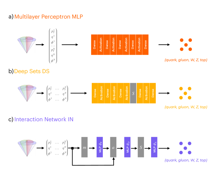
Figure 1: Schematic of all the considered model architectures. (a) A simple multilayer perceptron. The two-dimensional input is flattened to one dimension before it is passed through the MLP. (b) A permutation-invariant deep set network [22]. The initial MLP acts on the features of each input constituent. The aggregation layer $S$ performs a permutation invariant operation at the constituent level, e.g., the average, and hence brings the input to a 1D vector. (c) A permutation-invariant interaction network [38] as proposed in Ref. [7]. The input is transformed by the marshaling function $m$ into a fully-connected graph. The exact mechanics of the IN are described in Section 3. For each network type, all hyperparameters, such as the number of layers and number of nodes per layer, are optimized depending on the number of constituents. The hyperparameters of each network are presented in Section 3, along with their performance in Table 1.

The output layer of the models consists of a fully-connected layer with five nodes and a softmax activation function which returns the predicted probabilities for an input jet to be part of each jet class. Based on the nature of the input data and the strict latency and resource constraints, we explore both simple MLP models and permutation-invariant DS and IN models. The former is considered due to their favorable low latency inference, whereas the latter are expected to have a higher classification accuracy since graphs and sets constitute a more natural representation. We compare the following architectures:

Table 1: Floating-point model performance for 8, 16, and 32 jet constituents.

Architecture	Constituents	Parameters	FLOPs	Accuracy	AUC
					$g$	$q$	$W$	$Z$	$t$
MLP	8	26,826	53,162	$64.6\pm 0.1\%$	0.84	0.88	0.90	0.88	0.92
DS		3,461	36,805	$64.0\pm 0.3\%$	0.84	0.88	0.90	0.88	0.92
IN		3,347	37,232	$64.9\pm 0.2\%$	0.84	0.88	0.91	0.89	0.92
MLP	16	20,245	40,485	$68.4\pm 0.3\%$	0.87	0.89	0.91	0.90	0.94
DS		3,461	71,109	$69.4\pm 0.2\%$	0.87	0.89	0.93	0.92	0.94
IN		3,347	140,432	$70.8\pm 0.2\%$	0.88	0.90	0.94	0.92	0.94
MLP	32	24,101	48,197	$66.2\pm 0.2\%$	0.90	0.89	0.89	0.88	0.94
DS		3,461	139,717	$75.9\pm 0.1\%$	0.91	0.91	0.96	0.95	0.95
IN		7,400	109,556	$75.8\pm 0.3\%$	0.91	0.91	0.96	0.95	0.95

1. A simple MLP as shown in Fig. 1(a). The natural representation of the data is two-dimensional and hence the input is flattened as it is passed through the network. The number of layers, number of nodes, and the other hyperparameters of the MLP varies based on the number of input constituents $N$. For 8 constituents, the MLP consists of eight layers with $\{120,60,32,64,64,64,32,44\}$ nodes, where we apply L1 regularization throughout with a coefficient of $1.31\times 10^{-5}$; this network is trained with a learning rate of $0.0013$ and batch size of $128$. In the 16 constituent case, the MLP has five layers with $\{88,88,44,44,44\}$ nodes and an L1 regularization coefficient of $2.36\times 10^{-5}$; the 16 constituent MLP is trained with a learning rate of $0.0015$ and batch size of $256$. Finally, for 32 constituents, the MLP is composed of 7 layers with $\{84,88,32,32,44,32,44\}$ nodes, has an L1 regularisation coefficient of $3.14\times 10^{-5}$, and is trained using a learning rate of $0.0047$ and a batch size of $1024$. All these three networks use the ReLU activation function [39, 40] and the Adam optimizer [41], where the learning rate is reduced by a factor of 10 every 15 epochs with no accuracy improvement. Early stopping is applied if no accuracy improvement is observed for 20 epochs.

2. A deep set network [22] as schematically illustrated in Fig. 1(b). The first MLP $\phi$ of this network acts on the features of each constituent independently, mapping the 3 input features to some output dimension $D$. Then, this output $A$ with dimensionality $(N,D)$ is aggregated by $S$ over the constituents $N$, reducing the data from a 2D matrix to a one dimensional vector of length $D$. Finally, a second MLP $\rho$ is applied to the aggregation output to produce the jet class predictions. For any $N\in\{8,16,32\}$, $\phi$ is comprised of 3 layers, each with 32 nodes. The aggregation $S$ is chosen to be an average instead of a maximum, since they give similar results, but it is trivial to compute the number of FLOPs for the average. The second MLP $\rho$ uses only one layer with 32 nodes, excluding the output layer. ReLU activation is used throught the three DS networks. The 8 and 16 constituent cases are trained with a batch size of 256 and learning rates of 0.0018 and 0.0029, respectively. Meanwhile, the 32 constituent DS is trained with a batch size of 128 and a rate of 0.0032. All the DS models use the same optimizer and optimization parameters as the MLP.

3. An interaction network [7, 38] that consists of an edge MLP $\phi_{R}$, followed by a node MLP $\phi_{O}$, and a graph classifier MLP $\phi_{A}$, as shown in Fig. 1(c). The $\phi_{R}$ network takes input features from a pair of nodes and learns a set of edge features. The edge features are aggregated at the corresponding “receiving” nodes, and concatenated with the original node features as input to $\phi_{O}$. The output embeddings are then averaged by $S$ over the $N$ constituents, and given as input to the graph classifier MLP, which consists of a single ReLU activated fully-connected layer, excluding the output layer. The $\phi_{R}$ and $\phi_{O}$ MLPs are implemented using 1D convolutions of unit kernel size and unit stride, where weights are shared across the edges and nodes. For 8 and 16 constituents, the edge MLP $\phi_{R}$ consists of $2$ layers with $\{12,6\}$ neurons. However, the $\phi_{R}$ for 32 constituents has only one layer with three neurons due to limited hardware resources. The node MLP $\phi_{O}$ comprises three layers with $\{36,18,6\}$ neurons for all the 3 cases. The graph classifier MLP $\phi_{A}$ have 170, 170, and 512 neurons for the 8, 16 and 32 constituent models, respectively. Both the IN models for 8 and 32 constituents are trained with a batch size of 128, while the batch size is 512 for the 16 constituent model. All the IN models use the Adam optimizer with a learning rate of 0.0005 and early stopping after 40 epochs of no validation accuracy improvement.

For all the models, Tensorflow version 2.8 and QKeras version 0.9 was used. The hyperparameter optimization constraints were set such that the model can fit on the chosen Xilinx Virtex UltraScale+ VU13P FPGA. Thus, the models presented in this work are not necessarily the best models that could be achieved with this data. However, they are the best possible models that can be synthesized on the chosen FPGA device. Additionally, pruning is applied to all the 32-constituent MLP, IN, and DS models such that they fit within the resource constraints of the FPGA. We prune the 32-constituent models using the TensorFlow Model Optimization Toolkit, with a polynomial decay schedule [42] and target sparsity of 50%. The pruning is only done for these type of models since the 32 constituent IN did not find on the chosen FPGA board right away. Conversely, the DS and MLP did, but for consistency across the 32 constituent models, they are pruned to 50% sparsity as well.

The performance of the models described above is shown in Table 1. The uncertainty on the AUC and FPR was studied using $k$-fold cross validation with $k=5$. The training dataset is split into 5 subsamples such that 1/5 is used for validation and the remaining 4/5 is used for training. The uncertainties on the figures of merit, AUC and FPR, are quantified by the standard deviation across the 5 folds and found to be $\mathcal{O}(0.1)\%$. However, the uncertainties due to random initalizations of model parameters are not quantified, but they would not impact the qualitative statements implied by our results.

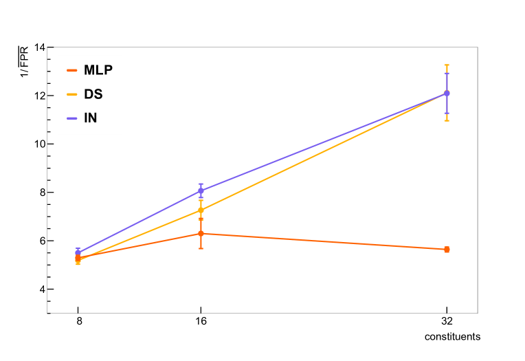
Figure 2: The inverse of the average false positive rate (FPR) at a fixed true positive rate (TPR) of 80% over $k=5$ folds of the data for $N\in\{8,16,32\}$ constituents per jet. This TPR was chosen to maximize the efficiency of identifying a potential signal. The size of the MLP is constrained by requiring it to be synthesizable in hls4ml. Therefore, the number of parameters per consecutive layer is limited and the MLP performance decreases from 16 to 32 constituents. This is not a factor for the other networks that use a 2D representation of the data. The models are quantized to 8 bits.

Figure 2 shows the inverse of the average FPR across classes at 80% TPR for each model as a function of the number of constituents. The models whose performance is shown in this figure are not the floating point models, but their weights and activations are quantized to 8 bits. The details of this quantization process are explained in Section 4. For now, notice that when the number of constituents is small, the architectures under study perform very similarly in terms of tagging accuracy. However, when increasing the input size up to 32 constituents, the DS and IN perform significantly better than MLPs. As the number of input constituents increases from 8 to 32, the IN and the DS have a higher inverse mistagging rate than the MLP, across all classes.

In addition, while the mistagging rate decreases significantly for the IN and DS as the number of input constituents increases, the mistagging rate increases for the MLP. One might assume that part of the reason the DS and IN perform better than the MLP for more constituents comes from the former having a larger effective capacity. However, increasing the size of the MLP, within the overall constraints imposed by the HLS compiler and the targeted FPGA, did not lead to an improvement in performance.

This implies that for an L1T system where more than 8 unordered jet constituents are available, using a set or a fully-connected graph representation is beneficial in terms of signal efficiency. As can be seen from Table 1, this is, however, at the cost of a significantly higher number of operations necessary for the DS or IN, which implies that the models come at a higher resource cost. Ultimately, a trade-off must be made between acceptable signal efficiency and tolerable resource and latency cost.

4 Model compression by quantization

We compress the aforementioned models through quantization, using QKeras [43, 15]. The quantization is performed using the straight-through estimator where layers are quantized during the forward pass, but not for backpropagation. The models are trained scanning the bit widths from 2 to 16, with the number of integer bits set to zero. Furthermore, all parameters are quantized to the same bit width. The quantized counterpart of each IN architecture is implemented using QKeras supported layers, such as fully-connected and convolutional layers. We also developed a custom Keras layer to project the features from the nodes to edges and vice versa through multiplication by the sending or receiving adjacency matrices.

The effect of quantization on the inverse false positive rate averaged over classes, 1/$\overline{\mathrm{FPR}}$, at a fixed TPR of 80% is shown in Figure 3 for the 8 constituent models. The uncertainty band is again estimated from the $k$-fold cross validation. The figure shows explicitly that 8-bit precision through quantization-aware training is sufficient to compress the models and simultaneously maintain high jet tagging accuracy for the architectures studied.

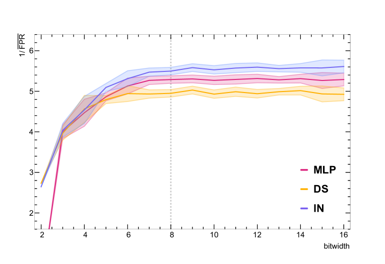
Figure 3: The inverted average FPR across the five jet classes, $1/\overline{\mathrm{FPR}}$, as a function of the bit width for the IN, DS, and MLP. For each model, the threshold on the classifier score corresponds to a TPR of 80%. A bit width of 8 maintains good classification accuracy while reducing the model resource consumption.

5 Firmware implementation

The quantized models are translated into firmware using hls4ml, then synthesized with AMD Vivado HLS 2020.1, targeting a Xilinx Virtex UltraScale+ VU13P (xcvu13p-flga2577-2-e) FPGA with a clock frequency of 200 MHz. We use a branch of hls4ml, available at Ref. [44]. Except for the custom projection layers in the IN model, all other layers are natively supported by hls4ml. For the projection layer, custom HLS was included using the extension API of hls4ml. Our custom HLS code is inspired by the optimizations in Ref. [33]. Since the adjacency matrices are binary, and the columns are one-hot encoded, multiplication and accumulation operations are eliminated. This simplifies the projection calculations to elementary load and store operations.

We also use a new parallelized implementation of pointwise 1D convolutional layers. Each pointwise layer runs an MLP on each jet constituent, requiring a total of $NM_{\mathrm{in}}M_{\mathrm{out}}$ multiplications where $N$ is the number jet constituents, $M_{\mathrm{in}}$ is the number of MLP inputs, and $M_{\mathrm{out}}$ is the number of MLP outputs. The amount of parallelization is controlled by the reuse factor (RF) in hls4ml, which is used to balance speed with resource consumption. The RF specifies how many times a multiplier unit is (re)used to compute all the multiplications in a given layer so that only $NM_{\mathrm{in}}M_{\mathrm{out}}/\mathrm{RF}$ total multiplier units are needed. To avoid a limitation of the HLS compiler on the number of fully unrolled elements within a function call, we split each layer computation into $N/\mathrm{RF}$ separate function calls each using only $M_{\mathrm{in}}M_{\mathrm{out}}$ multiplier units.

We first evaluate the FPGA latency and resource consumption for the three different architecture types at a numerical precision of 4, 6, and 8 bits. Table 2 shows the latency and resource consumption of these quantized models trained on jets with at most 8 constituents. The resources on the FPGA are digital signal processors (DSPs), lookup tables (LUTs), block random access memory (BRAM), and also flip-flops (FFs). The agreement between the FPGA and the CPU accuracy is larger than 90% for all the models studied.

Table 2: Average latency, initiation interval (II), and resource consumption for the MLP, DS, and IN models quantized to a bit width of 4, 6, and 8, trained on jet data with a maximum of 8 constituents. The $\mathrm{cc}$ next to the latency and II represents the number of clock cycles on the FPGA. The numbers in parentheses next to the FPGA resource values correspond to the used percentage of the given resource. The accuracy ratio between the models presented in this table and the quantized models before FPGA implementation are all above 0.9.

FPGA: Xilinx Virtex UltraScale+ VU13P
Architecture	Precision	RF	Latency [ns] (cc)	II [ns] (cc)	DSP	LUT	FF	BRAM18
MLP	4	1	95 (19)	5 (1)	101 (0.8%)	235,080 (13.6%)	90,150 (2.6%)	4 (0.1%)
	6	1	95 (19)	5 (1)	292 (2.4%)	313,371 (18.3%)	114,712 (3.3%)	4 (0.1%)
	8	1	105 (21)	5 (1)	262 (2.1%)	155,080 (7.6%)	25,714 (0.6%)	4 (0.1%)
DS	4	2	95 (19)	15 (3)	101 (0.8%)	235,359 (13.6%)	90,190 (2.6%)	4 (0.1%)
	6	2	95 (19)	15 (3)	292 (2.4%)	313,230 (18.1%)	114,745 (3.3%)	4 (0.1%)
	8	2	95 (19)	15 (3)	626 (5.1%)	386,294 (22.3%)	121,424 (3.5%)	4 (0.1%)
IN	4	2	150 (30)	10 (2)	5 (0.0%)	276,720 (16.0%)	124,354 (3.6%)	12 (0.2%)
	6	2	155 (31)	15 (3)	673 (5.5%)	387,625 (22.4%)	161,685 (4.7%)	12 (0.2%)
	8	2	160 (32)	15 (3)	2,191 (17.8%)	472,140 (27.3%)	191,802 (5.5%)	12 (0.2%)

Table 3: Number of jet constituents, reuse factor, latency, initialization interval (II) and resource consumption for the models quantized to 8 bits. The $\mathrm{cc}$ next to the latency and II represents the number of clock cycles on the FPGA. The numbers in parentheses next to the FPGA resource values correspond to the used percentage of the given resource. The accuracy ratio between the models presented in this table and the quantized models before FPGA implementation are all above 0.9.

FPGA: Xilinx Virtex UltraScale+ VU13P
Architecture	Constituents	RF	Latency [ns] (cc)	II [ns] (cc)	DSP	LUT	FF	BRAM18
MLP	8	1	105 (21)	5 (1)	262 (2.1%)	155,080 (9.0%)	25,714 (0.7%)	4 (0.1%)
	16	1	100 (20)	5 (1)	226 (1.8%)	146,515 (8.5%)	31,426 (0.9%)	4 (0.1%)
	32a	1	105 (21)	5 (1)	262 (2.1%)	155,080 (7.2%)	25,714 (0.7%)	4 (0.1%)
DS	8	2	95 (19)	15 (3)	626 (5.1%)	386,294 (22.3%)	121,424 (3.5%)	4 (0.1%)
	16	4	115 (23)	15 (3)	555 (4.5%)	747,374 (43.2%)	238,798 (6.9%)	4 (0.1%)
	32a	8	130 (26)	10 (2)	434 (3.5%)	903,284 (52.3%)	358,754 (10.4%)	4 (0.1%)
IN	8	2	160 (32)	15 (3)	2,191 (17.8%)	472,140 (27.3%)	191,802 (5.5%)	12 (0.2%)
	16	4	180 (36)	15 (3)	5,362 (43.6%)	1,387,923 (80.3%)	594,039 (17.2%)	52 (1.9%)
	32a	8	205 (41)	15 (3)	2,120 (17.3%)	1,162,104 (67.3%)	761,061 (22.0%)	132 (2.5%)

• Pruning to a sparsity of 50% is applied to the 32-constituent IN model such that it can fit within the resource constraints of the FPGA. For consistency, the same pruning sparsity is applied to the 32-constituent MLP and DS models.

A fully parallel implementation for all MLPs by setting the RF in hls4ml to 1, such that each network multiplication is distributed across all the resources. For the DS and IN models, the $\mathrm{RF}\in\{2,4,8\}$ for $N\in\{8,16,32\}$ constituents, respectively, due to the limited amount of hardware resources. Increasing the RF reduces the model resource consumption at the cost of increasing its latency and throughput. Equally important for the throughput is the initiation interval (II), which represents how many clock cycles it takes before the network is ready to receive new inputs. The II is higher for the DS and IN models. This can be partially compensated by running several instances of the model in parallel, but given their size, this might be infeasible. Additionally, an event contains multiple jets and thus deploying several versions of the same model to perform inference in parallel is necessary. Assuming 6 FPGA boards are used and 10 jets are classified per sequentially event, $\mathrm{II}\approx 15$ ns consistent with Table 3.

Table 3 shows how resource consumption and latency scale as a function of the number of input jet constituents for the three different architectures. While the latency remains relatively unchanged as the number of constituents increases for the MLP, the latency is proportional to the number of constituents for the DS and IN. For cases where the number of constituents is large, using a DS or IN architecture is advantageous. However, from Table 3, this incurs additional resources and latency. One solution to this resource problem is to use pruning [45, 14, 42, 46, 47, 48, 49], where insignificant weights are removed. When the model is synthesized, the pruned weights are set to zero and the corresponding operations are skipped. Different pruning algorithms [46, 47, 48] might yield better results. Alternatively, the reuse factor could be increased, but again, the gain of lower resource consumption comes at the cost of even higher inference latencies. Exploration of additional model compression paradigms is left for future work.

6 Conclusion and future work

Neural network based jet classification algorithms are implemented on devices that simulate the environment within the hardware layers of the real-time data processing systems for a typical LHC experiment after high-luminosity upgrades. Using jet data with constituent level information, we show how one could deploy machine learning algorithms pertaining to three different data representations on an FPGA using the hls4ml library. We also demonstrate how metrics like accuracy, latency, and resource, utilization scale as a function of the number of input jet constituents: an improvement in accuracy is gained by using a set or fully-connected graph representation when the number of jet constituents is larger than 8.

The Deep Sets network strikes a good balance between accuracy, latency, and resource consumption compared with the implemented and tested MLP and IN models. Employing quantization-aware training and, for the 32 constituent case, pruning, we also demonstrate how to efficiently limit resource utilization while retaining accuracy.

In conclusion, we have identified and shown the necessary ingredients to deploy a jet classifier in the level-1 trigger of the high-luminosity LHC experiments, when high-granularity particle information and particle-flow reconstruction would be accessible. An algorithm of this kind could significantly improve the quality of the trigger decision and improve signal acceptance, increasing the scientific reach of the experiments. Furthermore, the results shown in this work could be improved upon by employing advanced model compression techniques, more thorough hyperparameter optimization, and better synthesis fine-tuning.

7 Data availability

The data used in this study are openly available at Zenodo at Ref. [35] under DOI 10.5281/zenodo.3602260. The software used in this study is also available at Zenodo at Ref. [44] under DOI 10.5281/zenodo.10553804.

8 Author information

8.1 Corresponding author

Correspondence and material requests can be emailed to P. Odagiu (podagiu@ethz.ch).

References

- [1] ATLAS Collaboration, “The ATLAS Experiment at the CERN Large Hadron Collider”, JINST 3 (2008) S08003, doi:10.1088/1748-0221/3/08/S08003.
- [2] D. Contardo et al., “Technical Proposal for the Phase-II Upgrade of the CMS Detector”, CMS Technical Proposal, 2015. doi:10.17181/CERN.VU8I.D59J.
- [3] CMS Collaboration, “The Phase-2 Upgrade of the CMS Level-1 Trigger”, CMS Technical Design Report, 2020.
- [4] CMS Collaboration, “Particle-flow reconstruction and global event description with the CMS detector”, JINST 12 (2017) P10003, doi:10.1088/1748-0221/12/10/P10003, arXiv:1706.04965.
- [5] M. Cacciari, G. P. Salam, and G. Soyez, “The anti- jet clustering algorithm”, JHEP 04 (2008) 063, doi:10.1088/1126-6708/2008/04/063, arXiv:0802.1189.
- [6] M. Cacciari, G. P. Salam, and G. Soyez, “FastJet User Manual”, Eur. Phys. J. C 72 (2012) 1896, doi:10.1140/epjc/s10052-012-1896-2, arXiv:1111.6097.
- [7] E. A. Moreno et al., “JEDI-net: a jet identification algorithm based on interaction networks”, Eur. Phys. J. C 80 (2020) 58, doi:10.1140/epjc/s10052-020-7608-4, arXiv:1908.05318.
- [8] H. Qu and L. Gouskos, “ParticleNet: Jet Tagging via Particle Clouds”, Phys. Rev. D 101 (2020), no. 5, 056019, doi:10.1103/PhysRevD.101.056019, arXiv:1902.08570.
- [9] D. Guest et al., “Jet Flavor Classification in High-Energy Physics with Deep Neural Networks”, Phys. Rev. D 94 (2016), no. 11, 112002, doi:10.1103/PhysRevD.94.112002, arXiv:1607.08633.
- [10] G. Kasieczka et al., “The Machine Learning landscape of top taggers”, SciPost Phys. 7 (2019) 014, doi:10.21468/SciPostPhys.7.1.014, arXiv:1902.09914.
- [11] J. Duarte et al., “Fast inference of deep neural networks in FPGAs for particle physics”, JINST 13 (2018), no. 07, doi:10.1088/1748-0221/13/07/P07027, arXiv:1804.06913.
- [12] Fast Machine Learning Lab Collaboration, “hls4ml”, 2018. https://fastmachinelearning.org/hls4ml/.
- [13] M. Courbariaux, Y. Bengio, and J.-P. David, “BinaryConnect: Training deep neural networks with binary weights during propagations”, in Advances in Neural Information Processing Systems, C. Cortes et al., eds., volume 28, p. 3123. Curran Associates, Inc., 2015. arXiv:1511.00363.
- [14] S. Han, H. Mao, and W. J. Dally, “Deep compression: Compressing deep neural networks with pruning, trained quantization and Huffman coding”, in 4th International Conference on Learning Representations, San Juan, Puerto Rico, May 2, 2016, Y. Bengio and Y. LeCun, eds. 2016. arXiv:1510.00149.
- [15] C. Coelho, “QKeras”, 2019. https://github.com/google/qkeras.
- [16] P. T. Komiske, E. M. Metodiev, and J. Thaler, “Energy Flow Networks: Deep Sets for Particle Jets”, JHEP 01 (2019) 121, doi:10.1007/JHEP01(2019)121, arXiv:1810.05165.
- [17] H. Qu, C. Li, and S. Qian, “Particle Transformer for Jet Tagging”, in Proceedings of the 39th International Conference on Machine Learning, K. Chaudhuri et al., eds., volume 162, p. 18281. 2022. arXiv:2202.03772.
- [18] Y. Iiyama et al., “Distance-Weighted Graph Neural Networks on FPGAs for Real-Time Particle Reconstruction in High Energy Physics”, Front. Big Data 3 (2020) 598927, doi:10.3389/fdata.2020.598927, arXiv:2008.03601.
- [19] A. Bogatskiy, T. Hoffman, D. W. Miller, and J. T. Offermann, “PELICAN: Permutation Equivariant and Lorentz Invariant or Covariant Aggregator Network for Particle Physics”, arXiv:2211.00454.
- [20] A. Bogatskiy et al., “Explainable Equivariant Neural Networks for Particle Physics: PELICAN”, arXiv:2307.16506.
- [21] S. Gong et al., “An efficient Lorentz equivariant graph neural network for jet tagging”, JHEP 07 (2022) 030, doi:10.1007/JHEP07(2022)030, arXiv:2201.08187.
- [22] M. Zaheer et al., “Deep sets”, in Advances in Neural Information Processing Systems, I. Guyon et al., eds., volume 30. Curran Associates, Inc., 2017. arXiv:1703.06114.
- [23] P. W. Battaglia et al., “Relational inductive biases, deep learning, and graph networks”, 2018. arXiv:1806.01261.
- [24] M. M. Bronstein, J. Bruna, T. Cohen, and P. Velvčković, “Geometric deep learning: Grids, groups, graphs, geodesics, and gauges”, 2021.
- [25] J. Zhou et al., “Graph neural networks: A review of methods and applications”, AI Open 1 (2021) 57, doi:10.1016/j.aiopen.2021.01.001, arXiv:1812.08434.
- [26] J. Shlomi, P. Battaglia, and J.-R. Vlimant, “Graph neural networks in particle physics”, Mach. Learn. Sci. Tech. 2 (2021) 021001, doi:10.1088/2632-2153/abbf9a, arXiv:2007.13681.
- [27] K. Guo et al., “A survey of FPGA-based neural network inference accelerators”, ACM Trans. Reconfigurable Technol. Syst. 12l (2018) doi:10.1145/3289185.
- [28] S. I. Venieris, A. Kouris, and C. Bouganis, “Toolflows for mapping convolutional neural networks on fpgas: A survey and future directions”, ACM Comput. Surv. 51 (2018), no. 3, doi:10.1145/3186332, arXiv:1803.05900.
- [29] S. Summers et al., “Fast inference of boosted decision trees in FPGAs for particle physics”, JINST 15 (2020), no. 05, P05026, doi:10.1088/1748-0221/15/05/p05026, arXiv:2002.02534.
- [30] T. M. Hong et al., “Nanosecond machine learning event classification with boosted decision trees in FPGA for high energy physics”, JINST 16 (2021) P08016, doi:10.1088/1748-0221/16/08/P08016, arXiv:2104.03408.
- [31] B. Carlson, Q. Bayer, T. M. Hong, and S. Roche, “Nanosecond machine learning regression with deep boosted decision trees in FPGA for high energy physics”, JINST 17 (2022) P09039, doi:10.1088/1748-0221/17/09/P09039, arXiv:2207.05602.
- [32] S. Roche et al., “Nanosecond anomaly detection with decision trees for high energy physics and real-time application to exotic Higgs decays”, arXiv:2304.03836.
- [33] Z. Que et al., “LL-GNN: Low Latency Graph Neural Networks on FPGAs for High Energy Physics”, ACM Trans. Embed. Comput. Syst. (2024) doi:10.1145/3640464.
- [34] B. Bhattacherjee, P. Konar, V. S. Ngairangbam, and P. Solanki, “LLPNet: Graph Autoencoder for Triggering Light Long-Lived Particles at HL-LHC”, arXiv:2308.13611.
- [35] J. M. Duarte et al., “hls4ml LHC jet dataset (150 particles)”, 2020. doi:10.5281/zenodo.3602260.
- [36] M. Abadi et al., “Tensorflow: Large-scale machine learning on heterogeneous systems”, 2015. Software available from tensorflow.org. https://www.tensorflow.org/.
- [37] F. Chollet et al., “Keras”, 2015. Software available from tensorflow.org. https://github.com/fchollet/keras.
- [38] P. W. Battaglia et al., “Interaction networks for learning about objects, relations and physics”, in Advances in Neural Information Processing Systems, D. Lee et al., eds., volume 29. Curran Associates, Inc., 2016. arXiv:1612.00222.
- [39] V. Nair and G. E. Hinton, “Rectified linear units improve restricted Boltzmann machines”, in Proc. of the 27th Int. Conf. on Machine Learning (ICML), p. 807. 2010.
- [40] X. Glorot, A. Bordes, and Y. Bengio, “Deep sparse rectifier neural networks”, in Proc. of the 14th Int. Conf. on Artificial Intelligence and Statistics (AISTATS), G. Gordon, D. Dunson, and M. Dudík, eds., volume 15, p. 315. 2011.
- [41] D. P. Kingma and J. Ba, “Adam: A method for stochastic optimization”, 2017.
- [42] M. Zhu and S. Gupta, “To prune, or not to prune: exploring the efficacy of pruning for model compression”, in 6th International Conference on Learning Representations, Workshop Track Proceedings. 2018. arXiv:1710.01878.
- [43] C. N. Coelho et al., “Automatic heterogeneous quantization of deep neural networks for low-latency inference on the edge for particle detectors”, Nature Mach. Intell. 3 (2021), no. 8, 675, doi:10.1038/s42256-021-00356-5, arXiv:2006.10159.
- [44] Z. Que, A. Sznajder, J. Duarte, and P. Odagiu, “l1-jet-id”, 2024. doi:10.5281/zenodo.10553804, https://github.com/fastmachinelearning/l1-jet-id.
- [45] Y. LeCun, J. S. Denker, and S. A. Solla, “Optimal brain damage”, in Advances in Neural Information Processing Systems, D. S. Touretzky, ed., volume 2, p. 598. Morgan-Kaufmann, 1990.
- [46] J. Frankle and M. Carbin, “The lottery ticket hypothesis: Finding sparse, trainable neural networks”, in 7th International Conference on Learning Representations. 2019. arXiv:1803.03635.
- [47] A. Renda, J. Frankle, and M. Carbin, “Comparing rewinding and fine-tuning in neural network pruning”, in 8th International Conference on Learning Representations, Addis Ababa, Ethiopia, April 26, 2020. 2020. arXiv:2003.02389. https://openreview.net/forum?id=S1gSj0NKvB.
- [48] H. Zhou, J. Lan, R. Liu, and J. Yosinski, “Deconstructing lottery tickets: Zeros, signs, and the supermask”, in Advances in Neural Information Processing Systems, H. Wallach et al., eds., volume 32, p. 3597. Curran Associates, Inc., 2019. arXiv:1905.01067.
- [49] D. Blalock, J. J. G. Ortiz, J. Frankle, and J. Guttag, “What is the state of neural network pruning?”, in Proceedings of Machine Learning and Systems, I. Dhillon, D. Papailiopoulos, and V. Sze, eds., volume 2, p. 129. 2020. arXiv:2003.03033.