Multi-Armed Bandits with Interference

Su Jia    Peter Frazier    Nathan Kallus
Abstract

Experimentation with interference poses a significant challenge in contemporary online platforms. Prior research on experimentation with interference has concentrated on the final output of a policy. The cumulative performance, while equally crucial, is less well understood. To address this gap, we introduce the problem of Multi-armed Bandits with Interference (MABI), where the learner assigns an arm to each of $N$ experimental units over a time horizon of $T$ rounds. The reward of each unit in each round depends on the treatments of all units, where the influence of a unit decays in the spatial distance between units. Furthermore, we employ a general setup wherein the reward functions are chosen by an adversary and may vary arbitrarily across rounds and units. We first show that switchback policies achieve an optimal expected regret $\tilde{O}(\sqrt{T})$ against the best fixed-arm policy. Nonetheless, the regret (as a random variable) for any switchback policy suffers a high variance, as it does not account for $N$. We propose a cluster randomization policy whose regret (i) is optimal in expectation and (ii) admits a high probability bound that vanishes in $N$.

Machine Learning, ICML

1 Introduction

Online controlled experiments (“A/B tests”) have become a standard practice for evaluating the impact of a new product or service change before wide-scale release. Although A/B tests work well in many situations, they often fail to provide reliable estimates in the presence of interference, where one unit’s treatment impacts another’s outcomes. For example, suppose a ride-sharing firm develops a new pricing algorithm. If the firm randomly assigns half of the drivers to the new algorithm, these drivers will alter their behaviors, which will impact the common pool of passengers and consequently the drivers not assigned the new algorithm.

Most previous work on experimentation with interference are focused on the quality of the final output, e.g., the mean-squared error of the estimator (e.g., Ugander et al. 2013) or the $p$-value in a hypothesis testing setting (e.g., Athey et al. 2018). On the other hand, the cumulative performance of AB testing policies is considerably important in practice, particularly considering the scale of these experiments on modern online platforms. However, this perspective is often overlooked.

This motivates us to study the aspect of cumulative reward maximization in A/B testing with interference. We employ a batched adversarial bandit framework where $N$ units (representing, for example, users in an online platform) lie on the $\sqrt{N}\times\sqrt{N}$ unit grid. We are given a set of $k$ treatment arms (or arms) and a time horizon with $T$ rounds. In each round, the learner assigns one arm to each unit and collects an observable reward.

The reward in each unit in each round is governed by a reward function, which is secretly chosen by an adversary at the beginning of the time horizon. As a key feature of our model, to capture interference, each reward function is determined by the treatments of all units, i.e., each reward function is defined on $[k]^{N}$ rather than on $[k]$.

Similarly to causal inference with network interference, efficient learning is impossible without additional structures. In line with reality, we assume that the unit-to-unit interference decreases in their (spatial) distance. Specifically, we employ Leung (2022)’s decaying interference property, which states that for any two assignments $w,w^{\prime}\in[k]^{N}$, their rewards at a unit are close if $w,w^{\prime}$ are identical on a ball-neighborhood of this unit. Moreover, the larger this neighborhood, the closer the values become.

1.1 Our Contributions

We contribute to the literature of multi-armed bandits and causal inference with interference in the following ways:
1. A Novel Formulation. We introduce the problem of Multi-Armed Bandits with Interference (MABI), bridging the field of experimentation under interference and online learning. In alignment with practices, we assume that the unit-to-unit interference level decays in distance. Our framework is fairly general, imposing no constraints on the non-stationarity or similarity in reward functions between units.
2. Optimal Expected Regret. We characterize the minimax expected regret as follows.
(a) Upper Bound. We show that any adversarial bandits policy induces a switchback policy (i.e., a policy that assigns all units the same arm in each round) for the MABI problem, with the same regret; see Proposition 3.2. In particular, the EXP3 policy for adversarial bandits induces a switchback policy with $\widetilde{O}(\sqrt{kT})$ expected regret; see Corollary 3.3.
(b) Lower Bound. We show that for any policy (possibly non-switchback), there is a two-armed MABI instance on which the policy suffers an $\Omega(\sqrt{T})$ regret in expectation; see Theorem 3.5. Interestingly, this suggests that $N$ does not help reduce the expected regret.
3. High Probability Regret Bound. Although the regret of a switchback policy may be optimal in expectation, it can suffer a high variance. To address this, we propose a policy that integrates (i) the EXP3-IX policy from adversarial bandits and (ii) the idea of clustered randomization from causal inference. The results involve the following components.
(a) The Robust Randomized Partition. Leung (2022) achieved optimal statistical performance using a uniform spatial clustering, in which each arm is assigned to each cluster with probability $p=\Theta(1)$. However, in our problem, $p$ may be exceptionally small due to weight updates, leading to an unfavorably high variance in the estimator. To address this, we introduce the Robust Randomized Partition which increases the worst-case exposure probability polynomially and consequently reduces the estimator’s variance.
(b) The HT-IX Estimator. To achieve a high probability regret bound, Kocák et al. (2014) modified the EXP3 policy by adding an implicit exploration (IX) parameter to the propensity weight. On the other hand, to estimate the average treatment effect under spatial interference, Leung (2022) proposed a Horvitz-Thompson (HT) type estimator for the (single-period) inference problem. We introduce the Horvitz-Thompson-IX (HT-IX) estimator which unifies these two estimators.
(c) High Probability Regret Bound. We show that the EXP3 policy based on the HT-IX estimator has a regret that (i) is optimal in expectation and (ii) admits a high-probability bound that vanishes in $N$; see Theorem 4.5. In contrast, the regret of any switchback policy does not vanish in $N$.

Finally, we emphasize that, from a practical perspective, the market size $N$ should be considered substantially greater than the number $T$ of rounds.

1.2 Related Work

Experimentation is a broadly-deployed learning tool in online commerce that is simple to execute (Kohavi & Thomke, 2017; Thomke, 2020; Larsen et al., 2023). As a key challenge, the violation of the so-called Stable Unit Treatment Value Assumption (SUTVA) has been viewed as problematic in online platforms (Blake & Coey, 2014). Many work that tackles this problem by assuming that interference is summarized by a low-dimensional exposure mapping and that units are individually randomized to treatment or control by Bernoulli or complete randomization (Manski, 2013; Toulis & Kao, 2013; Aronow & Samii, 2017; Basse et al., 2019; Forastiere et al., 2021).

To improve estimator precision, some work departed from unit-level randomization and introduced cluster correlation in treatment assignments (Ugander et al., 2013; Jagadeesan et al., 2020; Leung, 2022, 2023). However, these works usually focus on the quality of the final output, such as the bias and variance of the estimator (Ugander et al., 2013; Leung, 2022) and $p$-values for hypotheses testing (Athey et al., 2018).

While existing literature has primarily focused on the final output, the cumulative performance remains less well understood. A natural framework is mult-armed bandits (MAB) (Lai et al., 1985). There are three lines of work in MAB that are most related to this work: (i) adversarial bandits, (ii) multiple-play bandits and (iii) combinatorial bandits.

Particularly related is the adversarial bandit problem. Many policies for adversarial bandits are built on the idea of weight update (Vovk, 1990; Littlestone & Warmuth, 1994), first introduced for the full-information setting (i.e., the best expert problem). Auer et al. (1995) considered the bandit feedback version and proposed a forced exploration version of the EXP3 policy. Stoltz (2005) observed that the policy achieves the optimal expected regret even without additional exploration.

High-probability bounds for adversarial bandits were first provided by Auer et al. (2002) and explored in a more generic way by Abernethy & Rakhlin (2009). In particular, the idea to reduce the variance of importance-weighted estimators has been applied in various forms (e.g., Ionides 2008; Bottou et al. 2013), and was first introduced to bandits by Kocák et al. (2014). Subsequently, Neu (2015) showed that this algorithm admits high-probability regret bounds.

Another closely related line is multiple-play bandits (Anantharam et al., 1987), where the learner plays multiple arms per round and observes each of their feedback. In these work, the number of arms played in each round can be viewed as the “$N$” in our problem (Chen et al., 2013; Komiyama et al., 2015; Lagrée et al., 2016). This problem should be distinguished from multi-agent bandits/RL (Kanade et al., 2012; Busoniu et al., 2008; Zhang et al., 2021), where agents interact independently , but in our problem, each “agent” behaves completely passively.

Finally, since reward function is defined on the hypercube $[k]^{V}$, our work is also related to combinatorial bandits (Cesa-Bianchi & Lugosi, 2012) where the action set is a subset of a binary hypercube. However, most work in this area consider linear objectives, where our reward functions are only assumed to satisfy the decaying interference assumption, which his much more general than linear functions. A recent line of work focus on combinatorial bandits with non-linear reward functions, however, most of these work either assumes a stochastic setting (Agrawal et al., 2017; Kveton et al., 2015), or consider an adversarial setting with a specialized class of reward functions, such as polynomial link functions (Han et al., 2021).

2 Formulation

We consider a batched adversarial bandits setting. We consider set $V$ of $N=|V|$ units, $T$ treatment decision rounds, and $k$ treatment arms. For each round $t\in[T]$ and unit $v\in V$ there is a reward function $Y_{vt}:[k]^{V}\rightarrow[0,1]$ that can depend on the treatment assignment $w\in[k]^{V}$ of all units, not just that of unit $v$. At each round, the learner selects a treatment assignment $W_{t}\in[k]^{V}$ for all $N$ units and observes a reward of $Y_{vt}(W_{t})$ for each unit $v\in V$.

The treatment assignment depends only on the past in the following sense. A policy $\pi=(\pi_{1},\dots,\pi_{T})$ (or, adaptive design) consist of mappings $\pi_{t}:([k]^{V}\times[0,1]^{V})^{t-1}\to\Delta([k]^{V})$ from a history of observations of treatment assignments and outcomes to a distribution on assignments of treatments for all units. In round $t$, $W_{t}$ is drawn from $\pi_{t}(W_{1},(Y_{v1}(W_{1}))_{v\in V},\dots,W_{t-1},(Y_{v,t-1}(W_{t-1}))_{v\in V})$. We aim to control the loss compared to the best fixed arm.

Definition 2.1 (Regret).

Regret is defined as ${\rm Reg}(W):=\max_{a\in[k]}\{{\rm Reg}(W,a)\},$ where for any arm $a\in[k]$ we let

$${\rm Reg}(W,a):=\sum_{t=1}^{T}\frac{1}{N}\sum_{v\in V}\left(Y_{vt}(a\cdot{\bf 1}^{N})-Y_{vt}(W_{t})\right).$$

Note that regret is random because $W$ is random. We therefore focus on bounding regret in expectation or, preferably, in high probability. The reward functions are chosen “secretly” in advance in the specific sense that our bounds on regret will hold for any reward function (possibly subject to some constraints we discuss next). Thus, the bounds will hold even for worst-case reward functions chosen by an adversary.

The Decaying Interference Property. In many applications, the effect of a treatment diffuses primarily through physical interaction, such as a promotion on a ride-sharing app or a discount on a food delivery platform. In these cases, it is natural to assume that the level of interference decays in the spatial distance.

To formalize, consider a $\sqrt{N}\times\sqrt{N}$ lattice graph whose vertices represent the units. For any $u,v\in V$, define the distance $h(u,v)$ as the number of “hops” between them. For any $r\geq 0$, the radius-$r$ (open) ball is defined as $B(v,r):=\{u\in V:h(u,v)<r\}$. For clarity, $B(v,r)$ does not contain units that are exactly $r$ hops away. In particular, we have $B(v,0)=\emptyset$ and $B(v,1)=\{u\}.$

Leung (2022) considered the following notion of decaying interference. Consider a reward function $Y_{vt}(\cdot)$. We assume that if two assignments are identical on a ball-neighborhood of $v$, then their function values are close. To formalize, we write $w_{S}=(w_{v})_{v\in S}$ for any $S\subseteq V$.

Definition 2.2 (Decaying Interference Property).

Let $\psi:[0,\infty)\rightarrow[0,\infty)$ be a non-increasing function. A function $f:[k]^{V}\rightarrow$ is said to satisfy the $\psi$-decaying interference property (abbreviated as the $\psi$-DIP) if for any $r\geq 0$ and $w,w^{\prime}\in[k]^{V}$ with $w_{B(v,r)}=w^{\prime}_{B(v,r)}$, we have

$$|f(w)-f(w^{\prime})|\leq\psi(r).$$

A MABI instance is said to have the $\psi$-DIP if every reward function $Y_{vt}(\cdot)$ satisfies the $\psi$-DIP. We will assume that $\psi(0)=1$ and $\psi(\sqrt{N})=0$. This loses no generality since, given any non-increasing $\widetilde{\psi}:[0,\infty)\rightarrow[0,\infty)$, we can rescale it by defining $\psi(r):=1-\frac{\widetilde{\psi}(0)-\widetilde{\psi}(r)}{{\rm TV}(\widetilde{\psi})}$ where ${\rm TV}(\widetilde{\psi}):=\widetilde{\psi}(0)-\lim_{r\rightarrow\infty}\widetilde{\psi}(r)$.

As an important special case, consider $\psi(r)={\bf 1}(r=0)$. With $r=1$, Definition 2.2 implies that $|Y_{ut}(w)-Y_{ut}(w^{\prime})|\leq\psi(1)=0$ for any $w,w^{\prime}$ identical on $B_{u}(1)=\{u\}$. In other words, $Y_{ut}(w)$ only depends on $w_{u}$. In causal inference, this condition is known as the Stable Unit Treatment Values Assumption (SUTVA).

3 Expected Regret

In this section, we show that the minimax expected regret for the MABI problem is $\widetilde{\Theta}(\sqrt{T})$. We will present an upper and lower bound respectively in two subsections.

3.1 Upper Bound

We observe that when restricted to the following policy class, the MABI problem is equivalent to adversarial bandits.

Definition 3.1 (Switchback Policy).

A policy $W=(W_{t})_{t\in[T]}$ is a switchback policy if there is an adversarial bandits policy $(A_{t})$ with $W_{t}=A_{t}\cdot{\bf 1}^{N}$ a.s. for each $t\in[T]$.

Moreover, this reduction preserves the regret.

Proposition 3.2 (Reduction to Adversarial Bandits).

Let $A=(A_{t})$ be an adversarial bandits policy with regret $r(T)$. Then, the MABI policy $W=(W_{t})$ given by $W_{t}=A_{t}\cdot{\bf 1}^{N}$ satisfies ${\rm Reg}(W)=r(T).$

Noticing that the EXP3 policy for adversarial bandits has $\widetilde{O}(\sqrt{kT})$ regret, we deduce the following.

Corollary 3.3 (Upper Bound on Expected Regret).

Let $W$ be the switchback policy induced by the EXP3 policy, then ${\rm Reg}(W)=\widetilde{O}(\sqrt{kT})$.

3.2 Lower Bound on the Expected Regret

We start by noting that the bound in Corollary 3.3 does not involve $N$. This is because a switchback policy treats the entire system as a whole, without taking $N$ into account. Can we improve the expected regret by considering $N$?

We answer this negatively. At first glance, one might assume that this could be proved by a reduction to the known $\Omega(\sqrt{T})$ lower bound for adversarial bandits, similar to how we obtained the upper bound in Section 3.1. However, such a reduction is not viable because it is far from obvious whether the lower bound instance satisfies the $\psi$-DIP. Specifically, given a function defined on two “corners” ${\bf 0},{\bf 1}$ of the hypercube $\{0,1\}^{V}$, it is not clear whether we can extend it to the entire domain subject to the $\psi$-DIP.

As a crucial element of the lower bound, we show that such an extension is always possible.

Lemma 3.4 (Key Lemma for the Lower Bound).

Let $G=(V,E)$ be a graph. Fix a node $O\in V$ and define $M=\max_{v\in V}h(O,v)+1$. Then, for any non-increasing $\psi:[0,M]\rightarrow[0,1]$ with $\psi(0)=1$ and $\psi(M)=0$, there exists a function $f:\{0,1\}^{V}\rightarrow[0,1]$ satisfying
i) the boundary condition: $f({\bf 0}^{V})=0,f({\bf 1}^{V})=1$, and
ii) the $\psi$-DIP: for any $w,w^{\prime}\in\{0,1\}^{V}$ with $w_{B(O,r)}=w^{\prime}_{B(O,r)}$ for some $r\geq 0$, we have $|f(w)-f(w^{\prime})|\leq\psi(r).$

We construct $f$ as follows.
Step 1: Define $f$ on basis vectors. For each $r=0,1,\ldots,M$, we define the basis vector $\sigma^{r}\in\{0,1\}^{V}$ where $\sigma^{r}_{v}={\bf 1}(h(0,v)<r)$ for each entry $v\in V.$ Define $f\left(\sigma^{r}\right):=1-\psi(r)$ for $r=0,\dots,M.$
Step 2: Extend $f$ to $\{0,1\}^{V}$. For each $w\in\{0,1\}^{V}$, define $f(w)=f(\sigma^{r_{\star}(w)})$ where $r_{\star}(w)=\max\{r\geq 0:w_{B(O,r)}={\bf 1}_{B(O,r)}\}$.

We briefly explain why $f$ satisfies the two properties claimed in Lemma 3.4. First, note that $f(\sigma^{0})=1-\psi(0)=0$ and $f(\sigma^{M})=1-\psi(M)=1$, and so (i) holds.

The proof of (ii) is more involved. For any $w,w^{\prime}\in\{0,1\}^{V}$ with $r_{\star}(w)\leq r_{\star}(w^{\prime})$, consider the largest ball centered at $O$ on which $w$ and $w^{\prime}$ “agree”. Formally, consider $\rho:=\max\{r\geq 0:w_{B(O,r)}=w^{\prime}_{B(O,r)}\}$. Then, we can show that $\rho\leq r_{\star}(w)$; see Claim 1 in Appendix A. Therefore,

$\displaystyle|f(w)-f(w^{\prime})|$ $\displaystyle=|(1-\psi(r_{\star}(w)))-(1-\psi(r_{\star}(w^{\prime})))|$
$\displaystyle=\psi(r_{\star}(w))-\psi(r_{\star}(w^{\prime}))$
$\displaystyle\leq\psi(r_{\star}(w))\leq\psi(\rho),$

which verifies (ii). We formalize this in Appendix B.

To proceed with obtaining the lower bound, we follow the same approach as the $\Omega(\sqrt{T})$ lower bound for adversarial bandits. This involves combining the probabilistic method with an anti-concentration bound, as detailed in Section 4 of Arora et al. 2012. Specifically, consider i.i.d. Bernoulli variables $Z_{t}\sim{\rm Ber}(1/2)$ where $t\in[T]$. For each $v\in V$, $t\in[T]$, define

$$Y_{vt}(w)=\frac{1}{2}+\left(Z_{t}-\frac{1}{2}\right)f(w),\quad\forall w\in\{0,1\}^{V}.$$

Then, by Lemma 3.4, $Y_{vt}(\cdot)$ satisfies the $\psi$-DIP. Moreover, for any $w\in\{0,1\}^{V}$, we have $\mathbb{E}_{Z}[Y_{vt}(w)]=\frac{1}{2}$, and hence the expected reward of any policy is $T/2$.

On the other hand, using anti-concentration bounds, we can show that in expectation (over the randomness in the instance and the policy), there exists a fixed-arm policy that accrues a total reward of $\frac{1}{2}T+\Omega(T)$. This gives the following lower bound.

Theorem 3.5 (Lower Bound on the Expected Regret).

Fix any integer $N>0$ and non-increasing $\psi:[0,\infty)\rightarrow[0,1]$ with $\psi(0)=1$ and $\psi(\sqrt{N})=0$. Then for any MABI policy $W$, there exists a two-armed MABI instance $\cal I$ satisfying the $\psi$-DIP such that ${\rm Reg}(W,{\cal I})=\Omega(\sqrt{T}).$

4 High Probability Regret Bound

While switchback policies can achieve optimal expected regret, a notable drawback is their disregard for $N$, preventing them from capitalizing on the market size. Consequently, the fluctuation of regret (as a random variable) remains unaffected by $N$, rendering it less appealing to risk-averse decision-makers.

To address this, we propose a policy that (i) has an $\tilde{O}(\sqrt{T})$ expected regret and (ii) admits a high probability regret that vanishes in $N$. Specifically, for any fixed time horizon $T$ and confidence level $\delta>0$, the tail mass above $\tilde{\Theta}(\sqrt{T})$ vanishes $N\rightarrow\infty$.

Our policy that integrates (i) the EXP3-IX policy from adversarial bandits and (ii) the idea of clustered randomization from causal inference. We first provide some background.

4.1 Background

The EXP3-IX Policy. Policies for adversarial bandits often rely on weights update (Vovk, 1990; Littlestone & Warmuth, 1994): In each round, an arm is selected with a probability proportional to its weight, which is in turn updated to penalize low rewards. However, with bandit feedback, we only observe the rewards of the selected arm, which poses a challenge for weight updates. The EXP3 policy addresses this by employing a reliable reward estimate, achieving an optimal $\tilde{O}(\sqrt{kT})$ expected regret against the best fixed arm.

Despite the optimality in expectation, the regret of the EXP3 policy is prone to high variance: The regret can be linear in $T$ w.p. $\Omega(1)$; see Note 1 in Chapter 11 of Lattimore & Szepesvári 2020. This is essentially because the estimator in EXP3 can have a high variance. To address this, Kocák et al. (2014) introduced an implicit exploration (“IX”) term in the propensity weight, which truncates the value of the estimator and consequently reduces its variance. Despite introducing an extra bias, Neu (2015) showed that a judicious selection of the IX parameter ensures a high probability regret bound, at the cost of (only) an additional $\widetilde{O}(\sqrt{T})$ regret.

Cluster-Randomization For Spatial Interference. Leung (2022) considered the inference problem under spatial interference, assuming the potential outcomes (i.e., reward functions in the terminology of MAB) satisfies the DIP. They partition the plane uniformly into square clusters and independently assigned treatments (arms) to each cluster. Under this design, their truncated HT type estimator achieves favorable bias and variance, both vanishing in $N$.

However, there are two main challenges for integrating the truncated HT estimator into the EXP3-IX framework. First, the basic spatial clustering that Leung (2022) analyzed is no longer “robust” since some arms may have very low probabilities due to weight updates, leading to a high variance in the estimator. Furthermore, it is unclear how to select the IX parameter in the batched setting due to the heterogeneity across units. Next, we tackle these two challenges.

4.2 Robust Randomized Partition

A key component of the truncated HT estimator in Leung 2022 is the exposure mapping, defined as the binary indicator of whether all units sufficiently close to a unit are assigned the same treatment.

Definition 4.1 (Exposure Mapping).

For each unit $v\in V$, round $t\in[T]$ and arm $a\in[k]$, the radius-$r$ exposure mapping is given by $X_{vta}^{r}(W)=\prod_{u\in B(v,r)}{\bf 1}(W_{u}=a).$ The exposure probability is defined as $p_{vta}^{r}=\mathbb{P}[X_{vta}^{r}=1]$.

Intuitively, this exposure mapping specifies whether the data from a unit is sufficiently reliable for our estimation. Therefore, to achieve favorable statistical performance, we prefer a high exposure probability.

When $p=\Omega(1)$, the uniform clustering works well. To see this, suppose $r$ is equal to the side length of the squares. Then, the exposure probability is at least $p^{4}=\frac{1}{16}$, since an $r$-ball intersects at most $4$ clusters.

However, in our setting, $p$ is subject to updates by the policy, and therefore $p^{4}$ may be very small. This leads to the removal of almost all data from units near the corner, resulting in a high variance in the estimation. We address this by introducing randomness into the partition: We will start with uniform clustering and randomly assign the units close to the boundary to one of the nearby clusters.

Refer to caption
Figure 1: Illustration of the RRP. The black lines are the boundary for the squares in the uniform clustering. We color the strips in green and quads in red. We randomly assign each strip to one of the two neighboring clusters; see $S^{\rm ver}_{ij}$ (colored dark green) as an example. Finally, we assign each quad (colored red) to one of the four nearby clusters with equal probabilities.
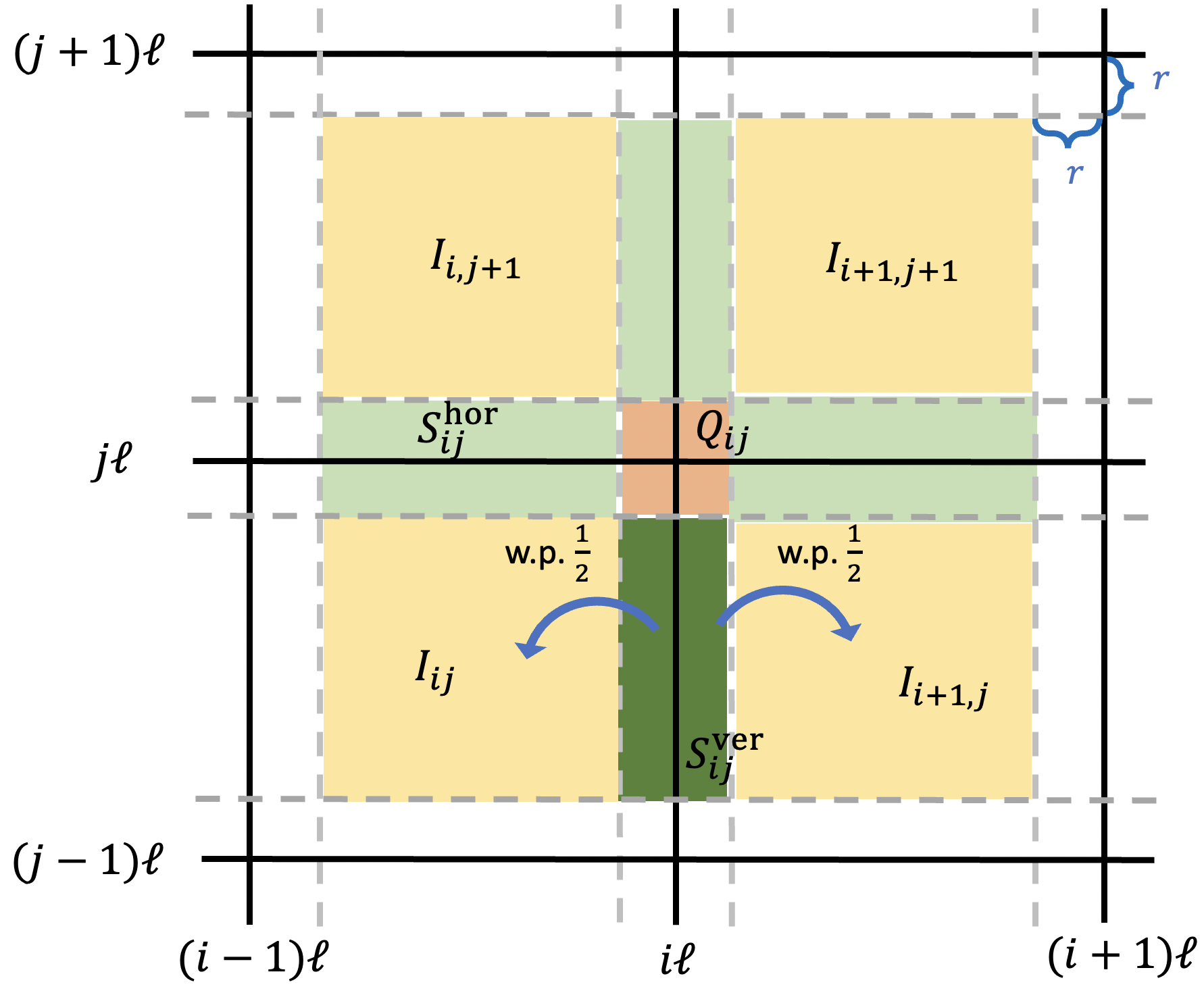
Definition 4.2 (Robust Randomized Partition).

Consider $[0,B]^{2}\subseteq^{2}$ for some $B>0$. For any $\ell,r>0$ with $\ell>2r$, an $(\ell,r)$-robust random partition (RRP) $\Pi=\{C_{ij}:1\leq i,j\leq\frac{B}{\ell}\}$ is defined as follows.
Step 1. Assign the Interiors: Define the $(i,j)$-interior as $I_{ij}=\left[(i-1)\ell+r,\ i\ell-r\right]\times\left[(j-1)\ell+r,\ j\ell-r\right].$ We assign $I_{ij}$ to $C_{ij}$ with probability $1$.
Step 2: Assign the strips: Define the vertical $(i,j)$-strip $S_{ij}^{\rm ver}=\left[i\ell-r,\ i\ell+r\right]\times\left[(j-1)\ell+r,\ j\ell-r\right],$ and the horizontal $(i,j)$-strip $S_{ij}^{\rm hor}=\left[(i-1)\ell+r,\ i\ell-r\right]\times\left[j\ell-r,\ j\ell+r\right].$ We randomly assign each $S^{\rm ver}_{ij}$ independently to $C_{ij}$ or $C_{i+1,j}$ uniformly. Similarly, assign $S^{\rm hor}_{ij}$ to independently to one of $C_{ij}$ and $C_{i,j+1}$ uniformly.
Step 3: Assign the quads: Define the $(i,j)$-quad $Q_{ij}=\left[i\ell-r,i\ell+r\right]\times\left[j\ell-r,j\ell+r\right]$ and assign it to one of $C_{ij},C_{i+1,j},C_{i,j+1}$ and $C_{i+1,j+1}$ uniformly.

We will consider the clustering of $V$ induced by $(\ell,r)$-RRP of $[0,\sqrt{N}]^{2}$, i.e., $\{V\cap C_{ij}\mid 1\leq i,j\leq\sqrt{N}/\ell\}$. By abuse of notation, we will abbreviate $V\cap C_{ij}$ as $C_{ij}$. For each $v\in V$, denote by $C[v]\subseteq V$ the unique cluster that contains $v$. From now on until Corollary 4.6, we will fix a pair of $\ell,r\geq 0$ with $1\leq\ell\leq\sqrt{N}$ and $2r<\ell$.

The RRP enjoys the following robustness.

Lemma 4.3 (Robustness of the RRP).

For any $v\in V$, we have $\mathbb{P}[B(v,r)\subseteq C[v]]\geq\frac{1}{16}$.

To see this, observe that $B(v,r)$ intersects at most $4$ regions (i.e., interiors, strips, or quads). Since each strip or quad is assigned to a cluster independently, w.p. $\Omega(1)$ these regions are all assigned to the same cluster $C$. When this occurs, we have $B(v,r)\subseteq C$. We defer the proof to Appendix C.

The above result helps us increase the worst-case exposure probability of each arm $a$ from $(P_{ta})^{4}$ to $\frac{1}{16}P_{ta}$. We will soon see how this helps reduce the variance of our estimator, which we define next.

4.3 HT-IX Estimator and Our Policy

The key to any adversarial bandits policy is to estimate the rewards of the arms which, in the context of the MABI problem, are $\{\bar{Y}_{t}(a\cdot{\bf 1}^{N})\}_{a\in[k]}$. Ideally, a good estimator should have both low bias and low variance. Neu (2015) showed that incorporating an additional IX parameter into the propensity weight results in a favorable high-probability regret bound. In the MABI problem, the propensity weights $Q_{vta}^{r}$ vary across units. However, a uniform IX parameter suffices for our result.

Definition 4.4 (Horvitz-Thompson-IX Estimator).

Suppose $\beta\in[0,\frac{1}{2})$. For each $t\in[T]$, $a\in[k]$ we define the Horvitz-Thompson-IX (HT-IX) estimator as

$$\widehat{Y}_{t}(a)=\frac{1}{N}\sum_{v\in V}\frac{{\bf 1}(X_{vta}^{r}(W_{t})=1)}{Q_{vta}^{r}+\beta}Y_{vt}(W_{t})$$

where $Q_{vta}^{r}=\mathbb{P}(X_{vta}^{r}(W_{t})=1)$.

Our HT-IX estimator “interpolates” between the estimators in Leung 2022 and Neu 2015: When $\beta=0$, it is the HT estimator in Leung 2022 (albeit with a more robust design), and when $N=1$, it becomes the estimator in the EXP3-IX policy Neu 2015.

We explain our policy in words and defer the statement to Algorithm 1. Our policy involves two parameters: The learning rate $\eta\in(0,1)$ controls how quickly we discount past data. The IX parameter $\beta\in[0,\frac{1}{2})$ caps the value of the HT-IX estimator under $1/\beta$. In each round, we independently generate an $(\ell,r)$-RRP. Then, we assign an arm to each cluster independently, drawn from a distribution determined by the weights. For each arm $a$, we use the HT-IX estimator to estimate the counterfactual reward that we could have earned if we assigned $a$ to all units in this round. Finally, we update the arm weights using the estimated rewards.

Algorithm 1 EXP3-HT-IX Policy
1:  Input: $\eta\in(0,1)$: learning rate,$\beta\in[0,\frac{1}{2})$: IX parameter for the HT-IX estimator,$(\ell,r)$: parameters for the RRP.
2:  $W_{ta}\leftarrow 1$ for each $a\in[k]$
3:  for $t=1,\dots,T$ do
4:     $W_{t}\leftarrow\sum_{a\in[k]}W_{ta}$
5:     For each arm $a\in[k]$, let $P_{ta}\leftarrow W_{ta}/W_{t}$
6:     Randomly generate an $(\ell,r)$-RRP $\Pi_{t}$
7:     for cluster $C\in\Pi_{t}$ do
8:        Draw an arm $A_{Ct}$ using $(P_{ta})_{a\in[k]}$
9:        for $v\in C$ do
10:           $W_{vt}\leftarrow A_{Ct}$
11:        end for
12:     end for
13:     Observe the rewards $\{Y_{vt}(W_{t})\}_{v\in V}$
14:     for $a\in[k]$ do
15:         $\widehat{Y}_{t}(a)\leftarrow\frac{1}{N}\sum_{v\in V}\frac{{\bf 1}(X_{vta}^{r}(W_{t})=1)}{Q_{vta}^{r}+\beta}Y_{vt}(W_{t})$
16:        $W_{t+1,a}\leftarrow e^{\eta\widehat{Y}_{t}(a)}W_{t,a}$
17:     end for
18:  end for

4.4 High Probability Regret Bound

We introduce some notation before stating our results. Given a policy $W=(W_{t})_{t\in[T]}$, the total reward per unit is $R=\sum_{t=1}^{T}\frac{1}{N}\sum_{v\in V}Y_{vt}(W_{t}).$ Since we are interested in comparing against a fixed arm $a\in[k]$, we also define the reward of the corresponding fixed-arm policy as $R_{a}:=\sum_{t=1}^{T}\bar{Y}_{t}(a)$ where $\bar{Y}_{t}(a):=\frac{1}{N}\sum_{v\in V}Y_{vt}(a\cdot{\bf 1}^{N})$.

All results stated hereafter involve fixed parameters $\delta\in(0,1)$, $\beta,\eta\in(0,1)$. Recall that an $(\ell,r)$-RRP has $m=N\ell^{-2}$ clusters.

Theorem 4.5 (Upper Bound).

For any $a^{*}\in[k]$, we have

$$R-R_{a^{*}}=A+B+C\quad\text{w.p. }1-\delta,$$
 $$\text{ where}\quad A\lesssim\frac{\log k}{\eta}+\eta T,\quad B\lesssim\left(\frac{1}{\beta}+\eta kT\right)\frac{1}{m}\log\frac{1}{\delta}$$
$$\text{and}\quad C\lesssim\beta kT+\frac{(r-1)T}{\ell}+\eta T\frac{k}{\beta}\psi(r)^{2}+\frac{T}{\beta\ell^{2}}\psi(r).$$

Choosing $\eta=\sqrt{\frac{\log k}{T}}$ and $\beta=\sqrt{\frac{\log\frac{1}{\delta}}{mT}}$, we obtain the following corollaries.

Corollary 4.6 (No Interference).

Suppose $\psi(r)={\bf 1}(r=0)$. Consider $\ell=O(1)$ and $r=1$. Then, for any $a^{*}\in[k]$,

$$R-R_{a^{*}}\lesssim\sqrt{kT\log k}+k\sqrt{\frac{T\log\frac{1}{\delta}}{N}}\quad\text{w.p. }1-\delta.$$

Another basic setting is where units can interfere up to a hop-distance of $h$ in the lattice graph (Leung, 2022).

Corollary 4.7 ($h$-Neighborhood Interference).

Suppose $\psi(r)={\bf 1}(h>r)$. Consider $r=h$ and $\ell=h\sqrt{T}$. Then, for any $a^{*}\in[k]$, we have

$$R-R_{a^{*}}\lesssim\sqrt{kT\log k}+khT\sqrt{\frac{\log\frac{1}{\delta}}{N}}\quad\text{w.p. }1-\delta.$$

Although the second term is linear in $T$, it will be dominated by $N$ in most practical settings, where $N$ is orders of magnitude larger than $T$.

Finally, we consider the setting where $\psi(r)$ follows the power law. This setting encompasses many fundamental settings, including the celebrated Cliff-Ord spatial autoregressive model (Cliff & Ord, 1973), which posits that each unit’s outcome is linear in its neighbors’ treatments; this connection has been made clear in Leung 2022.

Corollary 4.8 (Power-law Interference).

Suppose $\psi(r)=O(r^{-c})$ for some constant $c>1$. Let $m=\min\{(N/T)^{\frac{2+c}{3+c}},\ N^{\frac{2c}{2c+1}}T^{-\frac{2c-1}{2c+1}}\}$, $\ell=\sqrt{N/m}$ and $r=\ell/\sqrt{T}$. Then, for any $a^{*}\in[k]$,

$$R-R_{a^{*}}\lesssim\sqrt{kT\log k}+k\sqrt{\frac{T\log\frac{1}{\delta}}{m}}\quad\text{w.p. }1-\delta.$$

For example, when $c=2$, we have $m=(N/T)^{4/5},$ and Corollary 4.8 gives a regret bound of

$$\widetilde{O}\left(\sqrt{kT}\right)+k\frac{T^{9/10}}{N^{2/5}}\sqrt{\log\frac{1}{\delta}}.$$

5 Proof Outline of Theorem 4.5

We now outline the analysis. We first decompose the regret using the following fake reward.

Definition 5.1 (Fake Reward).

For each arm $a\in[k]$, we define $\widehat{R}_{a}=\sum_{t\in[T]}\widehat{Y}_{t}(a)$. We define the fake reward as $\widehat{R}=\sum_{t\in[T]}\sum_{a\in[k]}P_{ta}\widehat{Y}_{t}(a)$.

We can then decompose the regret using the fake reward. For any arm $a\in[k]$, we have

$$R-R_{a}=(R-\widehat{R})+(\widehat{R}-\widehat{R}_{a})+(\widehat{R}_{a}-R_{a}).$$

We bound these three terms separately in three subsections.

5.1 Bounding the First Term

Lemma 5.2 (Bounding $R-\widehat{R}$).

It holds that $R-\widehat{R}\leq\beta\sum_{a\in[k]}\widehat{R}_{a}+\frac{4rT}{\ell}.$

The $4rT/\ell$ term arises since there is at most a $4r/\ell$ proportion of the units that lie within a distance $r$ to their respective clusters. We defer the proof to Appendix D.

5.2 Bounding the Second Term

We need the following tool, stated as Lemma 12.2. in Lattimore & Szepesvári 2020.

Proposition 5.3 (One-sided Cramer-Chernoff Bound).

Let $\beta>0$ and $\mathbb{F}=(\mathcal{F}_{t})$ be a filtration. Let $\{z_{t\alpha}\}_{t\in[T],\alpha\in{\cal A}}$ be real numbers where $\cal A$ is the index set. Let $(\varepsilon_{t\alpha})$ be an $\mathbb{F}$-predictable process and $(Z_{t\alpha})$ be an $\mathbb{F}$-adapted process. Suppose $(Z_{t\alpha})$ are
(i) unbiased: $\mathbb{E}[Z_{t\alpha}|{\cal F}_{t-1}]=z_{t\alpha}$ for each $t\in[T],\alpha\in{\cal A}$,
(ii) negative correlated: $\mathbb{E}[\prod_{a\in S}Z_{t\alpha}|\mathcal{F}_{t-1}]\leq 0$ for any $t\in[T]$ and $S\subseteq\cal A$ with $|S|>1$, and
(iii) reasonably bounded: $0\leq\beta Z_{t\alpha}\leq 2\varepsilon_{t\alpha}$ a.s. for any $t\in[T]$ and $\alpha\in{\cal A}$.
Then, for any $\delta\in(0,1)$, we have

$$\mathbb{P}\left[\sum_{t\in[T]}\sum_{\alpha\in\cal A}\beta\left(\frac{Z_{t\alpha}}{1+\varepsilon_{t\alpha}}-z_{t\alpha}\right)\geq\log\frac{1}{\delta}\right]\leq\delta.$$

A natural idea is to apply the above with clusters in the role of $\alpha$ and time in the role of $t$. Specifically, for a fixed RRP $\Pi$, let us decompose $\widehat{Y}_{t}(a)$ as a sum over the clusters, by writing

$\displaystyle\widehat{Y}_{t}(a)=\frac{1}{N}\sum_{v\in V}\frac{{\bf 1}(X_{vta}^{r}=1)}{Q_{vta}^{r}+\beta}Y_{vt}(W_{t})=\frac{1}{N}\sum_{C\in\Pi}Z_{Ct}$
$$\text{where}\quad Z_{Cta}:=\sum_{v\in C}\frac{{\bf 1}(X_{vta}^{r}=1)}{Q_{vta}^{r}+\beta}Y_{vt}(W_{t}).$$

However, the negative correlation condition (ii) does not hold in general. In fact, consider two neighboring clusters $C,C^{\prime}\in\Pi$ and units $v\in C$ and $v^{\prime}\in C^{\prime}$ with $B(v,r)\cap B(v^{\prime},r)\neq\emptyset$. Then, for any $a\in[k]$, the exposure mappings $X_{vta}^{r}$ and $X_{v^{\prime}ta}^{r}$ are positively correlated and therefore $Z_{Cta}$ and $Z_{C^{\prime}ta}$ are dependent.

We avoid this obstacle by coloring the clusters so that the $Z_{Cta}$ terms of the clusters $C$ of the same color are independent. Specifically, we assign each cluster with one of $9$ colors such that $C_{ij}$ and $C_{i^{\prime}j^{\prime}}$ have the same color if and only if $(i,j)$ and $(i^{\prime},j^{\prime})$ have the same remainder when divided by $3$.

Definition 5.4 (Checkerboard Nine-Coloring).

Fix an $(\ell,r)$-RRP $\Pi$ of $[0,B]^{2}$. A mapping $\chi:\Pi\rightarrow\{0,1,2\}^{2}$ is a valid checkerboard $9$-coloring if for any $(i,j)$, $(i^{\prime},j^{\prime})$, we have $\chi(C_{ij})=\chi(C_{i^{\prime}j^{\prime}})$ if and only if $i\equiv i^{\prime}$ and $j\equiv j^{\prime}$ (mod $3$).

We show that two clusters of the same color have independent contributions to the estimator $\widehat{Y}_{t}(a)$.

Lemma 5.5 (Independence within Color Class).

Let $\chi$ be a checkerboard $9$-coloring of an $(\ell,r)$-RRP $\Pi$. Then, for any $C,C^{\prime}\in\Pi$ with $\chi(c)=\chi(c^{\prime})$, and $v\in C,v^{\prime}\in C^{\prime}$, we have $Z_{Cta}\perp Z_{C^{\prime}ta}$ for all $a\in[k]$.

To see this, note that each $Z_{Cta}$ is determined by the arm assigned to the clusters. Formally, conditional on the history up to the $(t-1)^{\rm st}$ round, $Z_{Cta}$ only depends on $\{A_{C^{\prime},t}\mid C^{\prime}\in\Gamma(C)\}$ where $\Gamma(C)=\{C^{\prime}\cap B(v,r)\neq\emptyset\text{ for some }v\in C^{\prime}\}$. Lemma 5.5 then follows by noticing that $Z_{Cta}$ and $Z_{C^{\prime}ta}$ are determined by two entirely different sets of random variables, i.e., $\Gamma(C)^{\prime}\cap\Gamma(C)=\emptyset$.

We use Lemma 5.5 and Proposition 5.3 to bound the deviation of $\widehat{R}_{a}$ from $R_{a}$. Recall that the number $m$ of clusters in an $(\ell,r)$-RRP for $[0,\sqrt{N}]^{2}$ satisfies $m\ell^{2}=N$.

Proposition 5.6 (Bounding $\widehat{R}_{a}-R_{a}$).

It holds that

$\displaystyle\widehat{R}_{a}-R_{a}\leq\frac{8}{\beta m}\log\frac{1}{\delta}+\frac{T}{\beta\ell^{2}}\psi(r)\quad\text{for all }a\in[k]$
$\displaystyle\text{and }\quad\sum_{a\in[k]}\left(\widehat{R}_{a}-R_{a}\right)\leq\frac{8}{\beta m}\log\frac{1}{\delta}+\frac{T}{\beta\ell^{2}}\psi(r).$

The proof entails addressing various technical intricacies, and we defer it to Appendix E.

5.3 Bounding the Third Term

We first derive an upper bound on $\widehat{R}-\widehat{R}_{a}$ by following the analysis of the EXP3 algorithm.

Lemma 5.7 (EXP3-style analysis).

Fix any $\eta\in(0,1)$. Then, for any $a\in[k]$, we have

$$\widehat{R}-\widehat{R}_{a}\leq\frac{\log k}{\eta}+\eta\sum_{t,a}P_{ta}\widehat{Y}_{t}(a)^{2}\quad\text{a.s.}$$

The proof is the same as in the analysis of the EXP3 analysis; see Equation (11.13) of Lattimore & Szepesvári 2020.

We next show that $\widehat{Y}_{t}(a)$ is highly concentrated around $\bar{Y}_{t}(a)$, with a tail mass that vanishes in $N$. This is done by a careful analysis based on the Chernoff and Bernstein inequalities and show the following in Section G.2.

Lemma 5.8 (Bounding the Squared Terms).

For any $\delta\in(0,1)$, with probability $1-\delta$ it holds that

$$\sum_{t,a}P_{ta}\widehat{Y}_{t}(a)^{2}\leq 512\left(1+\frac{k}{m}\log\frac{1}{\delta}+\frac{k}{\beta}\psi(r)^{2}\right)T.$$

5.4 Proof of Theorem 4.5

To highlight the key quantities, from now on we suppress the constants: By writing $A\lesssim B$, we mean $A=O(B)$. Fix $\delta>0$. Then, by Lemma 5.2,

$\displaystyle R-\widehat{R}$ $\displaystyle\lesssim\beta\sum_{a\in[k]}\widehat{R}_{a}+\frac{rT}{\ell}$
$\displaystyle=\beta\sum_{a\in[k]}R_{a}+\beta\sum_{a\in[k]}(\widehat{R}_{a}-R_{a})+\frac{rT}{\ell}$
$\displaystyle\leq\beta kT+\beta\sum_{a\in[k]}(\widehat{R}_{a}-R_{a})+\frac{rT}{\ell}.$ (1)

By Lemma 5.7 and Lemma 5.8, w.p. $1-\delta$ we have

$\displaystyle\widehat{R}-\widehat{R}_{a^{*}}\leq\frac{\log k}{\eta}+\eta\sum_{t,a}P_{ta}\widehat{Y}_{t}(a)^{2}$
$\displaystyle\lesssim\frac{\log k}{\eta}+\eta T\left(1+\frac{k}{m}\log\frac{1}{\delta}+\frac{k}{\beta}\psi(r)^{2}\right).$ (2)

Combining by combining Sections 5.4 and 5.4, we obtain

$\displaystyle R-R_{a^{*}}$ $\displaystyle=(R-\widehat{R})+(\widehat{R}-\widehat{R}_{a^{*}})+(\widehat{R}_{a^{*}}-R_{a^{*}})$
$\displaystyle\lesssim\beta kT+\beta\sum_{a\in[k]}(\widehat{R}_{a}-R_{a})+\frac{rT}{\ell}$
$\displaystyle\quad+\frac{\log k}{\eta}+\eta T\left(1+\frac{k}{m}\log\frac{1}{\delta}+\frac{k}{\beta}\psi(r)^{2}\right)$
$\displaystyle\quad+(\widehat{R}_{a^{*}}-R_{a^{*}})$
$\displaystyle\lesssim\beta kT+\frac{rT}{\ell}$
$\displaystyle\quad+\frac{\log k}{\eta}+\eta T\left(1+\frac{k}{m}\log\frac{1}{\delta}+\frac{k}{\beta}\psi(r)^{2}\right)$
$\displaystyle\quad+\frac{1}{\beta m}\log\frac{1}{\delta}+\frac{T}{\beta\ell^{2}}\psi(r),$ (3)

where the last inequality follows from Proposition 5.6 and that $\beta\leq 1$. The statement follows by rearranging the terms into three categories: (i) those that involve $\log\frac{1}{\delta}$, (ii) those that do not involve $\log\frac{1}{\delta}$ but involve $\eta$, and (iii) others.∎

6 Conclusions

We introduced the MABI problem as a batched MAB with interference in each batch, subject to a decaying interference condition. Although the availability of multiple units in each batch cannot reduce the expected regret compared to treating the batch as a single unit, as in a “pure” switchback experiment, we show it can significantly reduce the variation in regret, which can be very significant, even linear. As the number of units grows large, we can leverage the opportunity to learn from multiple units to attenuate the stochastic variations in regret. These developments bring together online learning and experimentation in the presence of interference. We believe this interface to be highly significant and hope this paper opens the door to future work dealing with the interaction of these challenges.

References

  • Abernethy & Rakhlin (2009) Abernethy, J. and Rakhlin, A. Beating the adaptive bandit with high probability. In 2009 Information Theory and Applications Workshop, pp. 280–289. IEEE, 2009.
  • Agrawal et al. (2017) Agrawal, S., Avadhanula, V., Goyal, V., and Zeevi, A. Thompson sampling for the mnl-bandit. In Conference on learning theory, pp.  76–78. PMLR, 2017.
  • Anantharam et al. (1987) Anantharam, V., Varaiya, P., and Walrand, J. Asymptotically efficient allocation rules for the multiarmed bandit problem with multiple plays-part i: Iid rewards. IEEE Transactions on Automatic Control, 32(11):968–976, 1987.
  • Aronow & Samii (2017) Aronow, P. M. and Samii, C. Estimating average causal effects under general interference, with application to a social network experiment. 2017.
  • Arora et al. (2012) Arora, S., Hazan, E., and Kale, S. The multiplicative weights update method: a meta-algorithm and applications. Theory of computing, 8(1):121–164, 2012.
  • Athey et al. (2018) Athey, S., Eckles, D., and Imbens, G. W. Exact p-values for network interference. Journal of the American Statistical Association, 113(521):230–240, 2018.
  • Auer et al. (1995) Auer, P., Cesa-Bianchi, N., Freund, Y., and Schapire, R. E. Gambling in a rigged casino: The adversarial multi-armed bandit problem. In Proceedings of IEEE 36th Annual Foundations of Computer Science, pp.  322–331. IEEE, 1995.
  • Auer et al. (2002) Auer, P., Cesa-Bianchi, N., Freund, Y., and Schapire, R. E. The nonstochastic multiarmed bandit problem. SIAM journal on computing, 32(1):48–77, 2002.
  • Basse et al. (2019) Basse, G. W., Feller, A., and Toulis, P. Randomization tests of causal effects under interference. Biometrika, 106(2):487–494, 2019.
  • Blake & Coey (2014) Blake, T. and Coey, D. Why marketplace experimentation is harder than it seems: The role of test-control interference. In Proceedings of the fifteenth ACM conference on Economics and computation, pp.  567–582, 2014.
  • Bottou et al. (2013) Bottou, L., Peters, J., Quiñonero-Candela, J., Charles, D. X., Chickering, D. M., Portugaly, E., Ray, D., Simard, P., and Snelson, E. Counterfactual reasoning and learning systems: The example of computational advertising. Journal of Machine Learning Research, 14(11), 2013.
  • Busoniu et al. (2008) Busoniu, L., Babuska, R., and De Schutter, B. A comprehensive survey of multiagent reinforcement learning. IEEE Transactions on Systems, Man, and Cybernetics, Part C (Applications and Reviews), 38(2):156–172, 2008.
  • Cesa-Bianchi & Lugosi (2012) Cesa-Bianchi, N. and Lugosi, G. Combinatorial bandits. Journal of Computer and System Sciences, 78(5):1404–1422, 2012.
  • Chen et al. (2013) Chen, W., Wang, Y., and Yuan, Y. Combinatorial multi-armed bandit: General framework and applications. In International conference on machine learning, pp. 151–159. PMLR, 2013.
  • Cliff & Ord (1973) Cliff, A. D. and Ord, J. K. Spatial autocorrelation. (No Title), 1973.
  • Forastiere et al. (2021) Forastiere, L., Airoldi, E. M., and Mealli, F. Identification and estimation of treatment and interference effects in observational studies on networks. Journal of the American Statistical Association, 116(534):901–918, 2021.
  • Han et al. (2021) Han, Y., Wang, Y., and Chen, X. Adversarial combinatorial bandits with general non-linear reward functions. In International Conference on Machine Learning, pp. 4030–4039. PMLR, 2021.
  • Ionides (2008) Ionides, E. L. Truncated importance sampling. Journal of Computational and Graphical Statistics, 17(2):295–311, 2008.
  • Jagadeesan et al. (2020) Jagadeesan, R., Pillai, N. S., and Volfovsky, A. Designs for estimating the treatment effect in networks with interference. 2020.
  • Kanade et al. (2012) Kanade, V., Liu, Z., and Radunovic, B. Distributed non-stochastic experts. Advances in Neural Information Processing Systems, 25, 2012.
  • Kocák et al. (2014) Kocák, T., Neu, G., Valko, M., and Munos, R. Efficient learning by implicit exploration in bandit problems with side observations. Advances in Neural Information Processing Systems, 27, 2014.
  • Kohavi & Thomke (2017) Kohavi, R. and Thomke, S. The surprising power of online experiments. Harvard business review, 95(5):74–82, 2017.
  • Komiyama et al. (2015) Komiyama, J., Honda, J., and Nakagawa, H. Optimal regret analysis of thompson sampling in stochastic multi-armed bandit problem with multiple plays. In International Conference on Machine Learning, pp. 1152–1161. PMLR, 2015.
  • Kveton et al. (2015) Kveton, B., Wen, Z., Ashkan, A., and Szepesvari, C. Combinatorial cascading bandits. Advances in Neural Information Processing Systems, 28, 2015.
  • Lagrée et al. (2016) Lagrée, P., Vernade, C., and Cappe, O. Multiple-play bandits in the position-based model. Advances in Neural Information Processing Systems, 29, 2016.
  • Lai et al. (1985) Lai, T. L., Robbins, H., et al. Asymptotically efficient adaptive allocation rules. Advances in applied mathematics, 6(1):4–22, 1985.
  • Larsen et al. (2023) Larsen, N., Stallrich, J., Sengupta, S., Deng, A., Kohavi, R., and Stevens, N. T. Statistical challenges in online controlled experiments: A review of a/b testing methodology. The American Statistician, pp.  1–15, 2023.
  • Lattimore & Szepesvári (2020) Lattimore, T. and Szepesvári, C. Bandit algorithms. Cambridge University Press, 2020.
  • Leung (2022) Leung, M. P. Rate-optimal cluster-randomized designs for spatial interference. The Annals of Statistics, 50(5):3064–3087, 2022.
  • Leung (2023) Leung, M. P. Network cluster-robust inference. Econometrica, 91(2):641–667, 2023.
  • Littlestone & Warmuth (1994) Littlestone, N. and Warmuth, M. K. The weighted majority algorithm. Information and computation, 108(2):212–261, 1994.
  • Manski (2013) Manski, C. F. Identification of treatment response with social interactions. The Econometrics Journal, 16(1):S1–S23, 2013.
  • Neu (2015) Neu, G. Explore no more: Improved high-probability regret bounds for non-stochastic bandits. Advances in Neural Information Processing Systems, 28, 2015.
  • Stoltz (2005) Stoltz, G. Incomplete information and internal regret in prediction of individual sequences. PhD thesis, Université Paris Sud-Paris XI, 2005.
  • Thomke (2020) Thomke, S. Building a culture of experimentation. Harvard Business Review, 98(2):40–47, 2020.
  • Toulis & Kao (2013) Toulis, P. and Kao, E. Estimation of causal peer influence effects. In International conference on machine learning, pp. 1489–1497. PMLR, 2013.
  • Ugander et al. (2013) Ugander, J., Karrer, B., Backstrom, L., and Kleinberg, J. Graph cluster randomization: Network exposure to multiple universes. In Proceedings of the 19th ACM SIGKDD international conference on Knowledge discovery and data mining, pp.  329–337, 2013.
  • Vovk (1990) Vovk, V. Aggregating strategies. In Proceedings of 3rd Annu. Workshop on Comput. Learning Theory, pp.  371–383, 1990.
  • Zhang et al. (2021) Zhang, K., Yang, Z., and Başar, T. Multi-agent reinforcement learning: A selective overview of theories and algorithms. Handbook of reinforcement learning and control, pp. 321–384, 2021.

Appendix A Proof of Lemma 3.4

Since we have verified (i) in the main body, here we focus on (ii). Suppose $w,w^{\prime}\in\{0,1\}^{V}$ satisfy $w_{B(O,r)}=w^{\prime}_{B(O,r)}$ for some $r\geq 0$. Wlog we assume that $r_{\star}:=r_{\star}(w)\leq r_{\star}^{\prime}:=r_{\star}(w^{\prime})$. We will need the crucial observation.

Claim 1. Let $\rho=\rho(w,w^{\prime})=\max\{r\geq 0:w_{B(O,r)}=w^{\prime}_{B(O,r)}\}$. Then, $\rho\geq r_{\star}$.

Proof.

Consider two cases. In the trivial case where $r_{\star}=r_{\star}^{\prime}=r$, the claim is clearly true. Now suppose $r_{\star}<r_{\star}^{\prime}$, i.e., $r_{\star}+1\leq r_{\star}^{\prime}$. Then, there exists $u\in B(O,r_{\star}+1)$ such that $w_{u}\neq w^{\prime}_{u}$. Therefore, $w^{\prime}_{B(O,r_{\star}^{\prime})}\neq w_{B(O,r_{\star}^{\prime})}$, thus $\rho<r_{\star}+1$. On the other hand, since $w^{\prime}_{B(O,r_{\star}^{\prime})}=w_{B(O,r_{\star}^{\prime})}={\bf 1}$. Therefore, $\rho=r_{\star}$. ∎

To conclude, note that

$$|f(w)-f(w^{\prime})|=|(1-\psi(r_{\star}))-(1-\psi(r_{\star}^{\prime}))|=\psi(r_{\star})-\psi(r_{\star}^{\prime})\leq\psi(r_{\star}).$$

Since $\rho\geq r_{\star}$ and $\psi$ is non-increasing, we have $\psi(r_{\star})\leq\psi(\rho)$, and the statement follows.∎

Appendix B Proof of Theorem 3.5

We need the following forklore anti-concentration bound; see, e.g., Lemma 4.2 of (Arora et al., 2012).

Lemma B.1 (Anti-concentration for Bernoulli Variables).

Let $(Z_{t})_{t\in[T]}$ be i.i.d. Bernoulli’s with mean $\frac{1}{2}$, and write $Z=\sum_{t=1}^{T}Z_{t}$. Then, for any $s\in[0,\frac{T}{8}]$, it holds that

$$\mathbb{P}\left[Z\leq\frac{T}{2}-s\right]\leq\frac{1}{15}\exp\left(-\frac{16s^{2}}{T}\right)$$

Now, we are ready to prove the lower bound. Recall that for each $v\in V$ and $t\in[T]$, we have defined

$\displaystyle Y_{vt}:\{0,1\}^{V}$ $\displaystyle\to[0,1]$
$\displaystyle w$ $\displaystyle\mapsto\frac{1}{2}+\left(Z_{t}-\frac{1}{2}\right)f(w),$

where $Z_{t}\sim{\rm Ber}(\frac{1}{2})$ for all $t\in[T]$ independently.

Proof of Theorem 3.5. By Lemma 3.4, the function $Y_{vt}(\cdot)$ satisfies the $\psi$-DIP. Moreover, for any fixed $w\in\{0,1\}^{V}$, we have $\mathbb{E}_{Z}[Y_{vt}(w)]=\frac{1}{2}$. Therefore, for any policy $W$, the total reward $R$ satisfies $\mathbb{E}_{Z}[R]=T/2$.

Next, we show that the best fixed arm policy has total reward much higher than $T/2$. Consider the event ${\cal E}=\{\left|Z-\frac{T}{2}\right|\geq\frac{\sqrt{T}}{4}\}$. Taking $s=\frac{1}{4}\sqrt{T}$ in Lemma B.1, we have $\mathbb{P}\left[{\cal E}\right]\geq\frac{1}{15}.$ Note that $\max\{R_{0},R_{1}\}\geq\frac{T}{2}$ a.s., so

$\displaystyle\mathbb{E}\left[\max\left\{R_{0},R_{1}\right\}\right]$ $\displaystyle=\mathbb{E}\left[\max\left\{R_{0},R_{1}\right\}\mid{\cal E}\right]\cdot\mathbb{P}[{\cal E}]+\mathbb{E}\left[\max\left\{R_{0},R_{1}\right\}\mid\bar{\cal E}\right]\cdot\mathbb{P}[\bar{\cal E}]$
$\displaystyle\geq 0\cdot 1+\frac{1}{4}\cdot\frac{\sqrt{T}}{15}$
$\displaystyle=\frac{\sqrt{T}}{60}.$

Appendix C Proof of Lemma 4.3.

Consider two cases.
Case 1. Suppose $B(v,r)$ intersects some interior, say $I_{ij}$. Then, $B(r,r)$ intersects at most $2$ strips and $1$ quad. The probability that these 3 regions are assigned to $C_{ij}$ is

$$\frac{1}{2}\times\frac{1}{2}\times\frac{1}{4}=\frac{1}{16}.$$

Case 2. Suppose $B(v,r)$ intersects no interior or strips. Then, $B(v,r)\subseteq Q$ for some quad $Q$ and hence $\mathbb{P}[B(v,r)\subseteq C[v]]=1.$
Case 3. Suppose $B(v,r)$ intersects no interior and exactly $1$ strip $S$. Then, it must also intersect some quad $Q$. Denote by $I_{\alpha_{1}},I_{\alpha_{2}}$ the two interiors that $S$ neighbors where $\alpha_{1},\alpha_{2}\in\{1,\dots,B/\ell\}^{2}$. Then,

$\displaystyle\mathbb{P}\left[B(v,r)\subseteq C[v]\right]$ $\displaystyle=\sum_{i=1,2}\mathbb{P}[S\subseteq C_{\alpha_{i}}]\cdot\mathbb{P}\left[Q\subseteq C_{\alpha_{i}}\mid S\subseteq C_{\alpha_{i}}\right]$
$\displaystyle=\frac{1}{2}\cdot\frac{1}{4}+\frac{1}{2}\cdot\frac{1}{4}=\frac{1}{4}.$

Case 4. Suppose $B(v,r)$ does not intersect any interior, and intersects $2$ strips, denoted $S,S^{\prime}$, and $1$ quad, denoted $Q$. Then, $S,S^{\prime}$ are neighboring the same interior, say $C_{ij}$. Then,

$$\mathbb{P}[B(v,r)\subseteq C_{ij}]=\mathbb{P}[S\subseteq C_{ij}]\cdot\mathbb{P}[S^{\prime}\subseteq C_{ij}]\cdot\mathbb{P}[Q\subseteq C_{ij}]=\frac{1}{16}.$$

The statement follows by combining the above four cases.∎

Appendix D Proof of Lemma 5.2

For convenience, we write

$$R=\sum_{t=1}^{T}R_{t}\quad\text{where}\quad\widehat{R}_{t}=\sum_{a\in[k]}P_{ta}\widehat{Y}_{t}(a),\quad\text{and}\quad\widehat{R}=\sum_{t=1}^{T}\widehat{R}_{t}\quad\text{where}\quad R_{t}=\frac{1}{N}\sum_{v\in V}Y_{vt}(W_{t}).$$

Now, fix any $t\in[T]$. Observe that the exposure mappings of a unit $v$ can only be all zero if $v$ lies close to $\partial C[v]$, i.e., the boundary of the cluster containing $c$. Thus,

$\displaystyle N(R_{t}-\widehat{R}_{t})$ $\displaystyle=\sum_{v,a}{\bf 1}(X^{r}_{vta}=1)Y_{ut}(A_{t})+\sum_{v\in V}{\bf 1}(X^{r}_{vt0}=X^{r}_{vt1}=0)-\sum_{v,a}\frac{P_{ta}}{Q_{vta}^{r}+\beta}{\bf 1}(X^{r}_{vta}=1)Y_{ut}(A_{t})$
$\displaystyle\leq\sum_{v,a}{\bf 1}(X^{r}_{vta}=1)Y_{ut}(A_{t})+\sum_{v\in V}{\bf 1}(d(v,\partial C[v])\leq r)-\sum_{v,a}\frac{P_{ta}}{P_{ta}+\beta}{\bf 1}(X^{r}_{vta}=1)Y_{ut}(A_{t}),$ (4)

where the inequality follows since $Q_{vta}\leq P_{ta}$. Note that in each cluster, there are at most $4r\ell$ units within a distance of $r$ to $\partial C[v]$. Since there are $N/\ell^{2}$ clusters, we have

$$\sum_{v\in V}{\bf 1}(d(v,\partial C[v])\leq r)\leq 4r\ell\cdot\frac{N}{\ell^{2}}=\frac{4rN}{\ell}.$$

It follows that

(D)italic-(Ditalic-)\displaystyle\eqref{eqn:012424} $\displaystyle=\sum_{v,a}\frac{\beta}{P_{ta}+\beta}{\bf 1}(X^{r}_{vta}=1)Y_{ut}(A_{t})+\frac{4rN}{\ell}$
$\displaystyle\leq\beta N\sum_{a\in[k]}\left(\frac{1}{N}\sum_{v\in V}\frac{{\bf 1}(X_{vta}^{r}=1)}{Q_{vta}^{r}+\beta}Y_{ut}(A_{t})\right)+\frac{4rN}{\ell}$
$\displaystyle=\beta N\sum_{a\in[k]}\widehat{Y}_{t}(a)+\frac{4rN}{\ell},$

where inequalities follows again from $Q_{vta}^{r}\leq P_{ta}$. Therefore,

$$N\left(R-\widehat{R}\right)=N\sum_{t=1}^{T}\left(R_{t}-\widehat{R}_{t}\right)\leq N\beta\sum_{a\in[k]}\widehat{R}_{a}+\frac{4rNT}{\ell},$$

and the statement follows by dividing both sides by $N$.∎

Appendix E Proof of Proposition 5.3

We first claim that $(M_{n})_{n\in[T]}$ is a super-martingale where $M_{n}:=\prod_{t=1}^{n}Z_{t}$. In fact, consider

$$Z_{t}=\exp\left(\sum_{\alpha\in{\cal A}}\beta\left(\frac{Z_{t\alpha}}{1+\varepsilon_{t\alpha}}-z_{t\alpha}\right)\right).$$

We first use the Cramer-Chernoff method to prove that $\mathbb{E}_{t-1}[Z_{t}]\leq 1$ for any $t\in[T]$. We will use the following fact: for any $x>0$, it holds that

$\displaystyle\exp\left(\frac{x}{1+\lambda}\right)\leq 1+x\leq e^{x}.$ (5)

Write $\mathbb{E}_{t}[\cdot]:=\mathbb{E}[\cdot|{\cal F}_{t}]$ for each $t\in[T]$. Then,

$\displaystyle\mathbb{E}_{t-1}\left[\exp\left(\sum_{\alpha\in{\cal A}}\frac{\beta Z_{t\alpha}}{1+\varepsilon_{t\alpha}}\right)\right]$ $\displaystyle=\mathbb{E}\left[\prod_{\alpha\in{\cal A}}\exp\left(\frac{\beta Z_{t\alpha}}{1+\varepsilon_{t\alpha}}\right)\right]$
$\displaystyle=\mathbb{E}\left[\prod_{\alpha\in{\cal A}}\left(1+\beta Z_{t\alpha}\right)\right]$ by the first inequality in eqn. (5)
$\displaystyle\leq\mathbb{E}\left[1+\beta\sum_{\alpha\in{\cal A}}Z_{t\alpha}\right]$ negative correlation
$\displaystyle=1+\beta\sum_{\alpha\in{\cal A}}z_{t\alpha}$ $\displaystyle\text{by unbiasedness of }Z_{t\alpha}$
$\displaystyle\leq\exp\left(\beta\sum_{\alpha\in{\cal A}}z_{t\alpha}\right)$ by the second inequality in Equation 5.by the second inequality in Equation 5\displaystyle\text{by the second inequality\ in \lx@cref{creftype~refnum}{eqn:112623}}.

Rearranging, we deduce that

$\displaystyle\mathbb{E}_{t-1}[Z_{t}]\leq 1$ (6)

Thus, for any $n\geq 1$, by the tower rule, we have

$$\mathbb{E}\left[\prod_{t=1}^{n}Z_{t}\right]=\mathbb{E}\left[\mathbb{E}_{n-1}\left[\prod_{t=1}^{n}Z_{t}\right]\right]=\mathbb{E}\left[\prod_{t=1}^{n}Z_{n}\cdot\mathbb{E}_{n-1}[Z_{t}]\right]\leq\mathbb{E}\left[\prod_{t=1}^{n-1}Z_{t}\right],$$

where the first equality follows from the tower rule, the second follows since $Z_{1},\dots,Z_{n-1}$ are $\mathcal{F}_{n-1}$-measurable, and the inequality is due to (6). By induction, we deduce that $\mathbb{E}\left[\prod_{t=1}^{n}Z_{t}\right]\leq 1$, and hence $(M_{t})$ is a super-martingale.

Finally, by Markov’s inequality, we conclude that

$$\mathbb{P}\left[\prod_{t=1}^{n}Z_{t}\geq\frac{1}{\delta}\right]\leq\mathbb{P}\left[M_{n}\geq\frac{1}{\delta}\mathbb{E}[M_{n}]\right]\leq\delta.$$

Appendix F Proof of Proposition 5.6

Denote by $N_{c}$ the (random) number of units in each cluster $c$, then $N_{c}\leq 2\ell^{2}$ a.s. Then,

$\displaystyle m(\widehat{R}_{a}-R_{a})$ $\displaystyle=\sum_{t=1}^{T}\sum_{C\in\Pi}\frac{1}{\ell^{2}}\sum_{v\in C}\left(\frac{{\bf 1}(X_{vta}^{r}=1)Y_{ut}(A_{t})}{Q_{vta}^{r}+\beta}-Y_{ut}(a\cdot{\bf 1})\right)$
$\displaystyle\leq\sum_{t=1}^{T}\sum_{C\in\Pi}\frac{1}{\ell^{2}}\sum_{v\in C}\left(\frac{{\bf 1}(X_{vta}^{r}=1)\cdot(Y_{ut}(a\cdot{\bf 1})+\psi(r))}{Q_{vta}^{r}+\beta}-Y_{ut}(a\cdot{\bf 1})\right)$
$\displaystyle=\sum_{t=1}^{T}\sum_{C\in\Pi}\frac{1}{\ell^{2}}\sum_{v\in C}\left(\frac{{\bf 1}(X_{vta}^{r}=1)Y_{ut}(a\cdot{\bf 1})}{Q_{vta}^{r}+\beta}-Y_{ut}(a\cdot{\bf 1})\right)+\sum_{t=1}^{T}\sum_{C\in\Pi}\frac{1}{\ell^{2}}\sum_{C\in\Pi}\frac{\psi(r)}{Q_{vta}^{r}+\beta}$
$\displaystyle\leq\sum_{t=1}^{T}\sum_{C\in\Pi}\frac{2}{N_{c}}\sum_{v\in C}\left(\frac{{\bf 1}(X_{vta}^{r}=1)}{1+\frac{\beta}{Q_{vta}^{r}}}Y_{ut}(a\cdot{\bf 1})-Y_{ut}(a\cdot{\bf 1})\right)+\frac{mT}{\beta\ell^{2}}\psi(r),$ (7)

where the first equality follows since $m\ell^{2}=N$, and the final inequality is because $Q_{vta}^{r}\geq 0$ and $N_{c}\leq 2\ell^{2}$ a.s. To apply Proposition 5.3, consider an unbiased estimate

$$\widetilde{Y}_{ut}(a):=\frac{{\bf 1}(X_{vta}^{r}=1)}{Q_{vta}^{r}}Y_{ut}(a\cdot{\bf 1}),$$

for $Y_{ut}(a\cdot{\bf 1})$. Then,

(F)italic-(Fitalic-)\displaystyle\eqref{eqn:011623} $\displaystyle=2\sum_{t=1}^{T}\sum_{C\in\Pi}\frac{1}{N_{c}}\sum_{v\in C}\left(\frac{1}{1+\frac{\beta}{Q_{vta}^{r}}}\widetilde{Y}_{ut}(a)-Y_{ut}(a\cdot{\bf 1})\right)+\frac{mT}{\beta\ell^{2}}\psi(r)$
$\displaystyle\leq 2\sum_{\kappa\in[4]}\sum_{t=1}^{T}\sum_{c:\chi(c)=\kappa}\left(\frac{1}{1+\frac{\beta}{P_{ta}}}\frac{1}{\ell^{2}}\left(\sum_{v\in C}\widetilde{Y}_{ut}(a)\right)-\bar{Y}_{ct}(a\cdot{\bf 1})\right)+\frac{mT}{\beta\ell^{2}}\psi(r),$

where the inequality is because $Q_{vta}^{r}\leq P_{ta}$.

We conclude by applying the Cramer-Chernoff inequality to the above sum. In Proposition 5.3, we take

$$Z_{t\alpha}:=\frac{1}{N_{c}}\sum_{v\in C}\widetilde{Y}_{ut}(a)\quad\text{and}\quad\varepsilon_{t\alpha}:=\frac{\beta}{P_{ta}}.$$

Then, condition (i) in Proposition 5.3 is satisfied since

$$\mathbb{E}[Z_{t\alpha}]=\mathbb{E}\left[\frac{1}{N_{c}}\sum_{v\in C}\widetilde{Y}_{ut}(a)\right]=\bar{Y}_{ct}(a\cdot 1).$$

Moreover, for each color $\kappa$, each term in the summation $\sum_{c:\chi(c)=\kappa}$ are independent, so (ii) is satisfied. Finally, note that for each $t,a$ we have

$$\beta Z_{t\alpha}=\beta\frac{1}{N_{c}}\sum_{v\in C}\widetilde{Y}_{ut}(a)=\beta\frac{1}{N_{c}}\sum_{v\in C}\frac{{\bf 1}(X_{vta}^{r}=1)}{Q_{vta}^{r}}Y_{ut}(a\cdot{\bf 1})\leq\frac{8\beta}{P_{ta}},$$

where the last inequality follows since $Q_{vta}^{r}\geq P_{ta}/8$ and $0\leq Y_{ut}(\cdot)\leq 1$. Therefore, by Proposition 5.3, we conclude that

$\displaystyle\beta m\left(\widehat{R}_{a}-R_{a}\right)$ $\displaystyle\leq 2\beta\sum_{\kappa\in[4]}\sum_{t=1}^{T}\sum_{c:\chi(c)=\kappa}\left(\frac{1}{1+\frac{\beta}{P_{ta}}}\frac{1}{N_{c}}\left(\sum_{v\in C}\widetilde{Y}_{ut}(a)\right)-\bar{Y}_{ct}(a\cdot{\bf 1})\right)+\frac{mT}{\ell^{2}}\psi(r)$
$\displaystyle\leq 8\log\frac{1}{\delta}+\frac{mT}{\ell^{2}}\psi(r),$

i.e.,

$$\widehat{R}_{a}-R_{a}\leq\frac{8}{\beta m}\log\frac{1}{\delta}+\frac{T}{\beta\ell^{2}}\psi(r).$$

The proof of (2) is identical by replacing every “$\sum_{v,t}$” with “$\sum_{v,t,a}$”. ∎

Appendix G Proof of Lemma 5.8

G.1 Preliminary Concentration Bounds

We need the following two basic concentration bounds for Bernoulli variables.

Theorem G.1 (Bernstein Inequality for i.i.d. Sum).

Let $\{Y_{i}\}_{i=1,\dots,n}$ be independent mean-zero random variables with $|Y_{i}|\leq M$ a.s. Then, for any $t>0$, we have

$$\mathbb{P}\left[\sum_{i=1}^{n}Y_{i}\geq t\right]\leq\exp\left(-\frac{t^{2}}{\sum_{i=1}^{n}\mathbb{E}[Y_{i}^{2}]+\frac{1}{3}Mt}\right).$$
Theorem G.2 (Chernoff Inequality for i.i.d. sum of Bernoulli’s).

Suppose $Z_{1},\dots,Z_{n}\sim{\rm Ber}(p)$ are iid random variables and $\bar{X}=\frac{1}{n}\sum_{i=1}^{n}Y_{i}$. Then, for any $\varepsilon>0$, we have

$$\mathbb{P}\left[\overline{X}\geq(1+\varepsilon)\right]\leq\exp\left(-\frac{1}{3}\varepsilon^{2}np\right).$$

Part (1). We will apply Bernstein’s inequality on $(Z_{i}-p)$. Since for each $i\in[n]$, we have $Z_{i}\in[0,1]$ a.s. and $\mathbb{E}[(Z_{i}-p)^{2}]={\rm Var}(Z_{i})\leq p$, by taking $M=1$ in Theorem G.1, we have

$\displaystyle\mathbb{P}\left[\sum_{i=1}^{n}Z_{i}\geq np+t\right]\leq\exp\left(-\frac{t^{2}}{\sum_{i=1}^{n}\mathbb{E}[(Z_{i}-p)^{2}]+\frac{1}{3}t}\right)\leq\exp\left(-\frac{t^{2}}{np+\frac{t}{3}}\right).$ (8)

for any $t$. Note that we have assumed that $p\geq\frac{1}{n}$, so for $t=\sqrt{2np\log\frac{1}{\delta}}$ we have $np>t$. It follows that

(8)exp(t22np)δ.italic-(8italic-)superscript𝑡22𝑛𝑝𝛿\eqref{eqn:112623b}\leq\exp\left(-\frac{t^{2}}{2np}\right)\leq\delta.

Part (2). It suffices to consider $\widetilde{Z}_{i}\sim{\rm Ber}(1/n)$ since $\sum_{i=1}^{n}\widetilde{Z}_{i}$ stochastically dominates $\sum_{i=1}^{n}Z_{i}$. By Chernoff bound (Theorem G.2), for any $\varepsilon>0$, we have

$$\mathbb{P}\left[\frac{1}{n}\sum_{i=1}^{n}\tilde{Z}_{i}\geq(1+\varepsilon)\cdot\frac{1}{n}\right]\leq\exp\left(-\frac{1}{3}\varepsilon^{2}n\cdot\frac{1}{n}\right).$$

In particular for $\varepsilon=\sqrt{3\log\frac{1}{\delta}}$, the above bound becomes $\delta$. ∎

Lemma G.3 (Deviation of Bernoulli Sum).

Suppose $\delta,p\in(0,1)$ and $Z_{1},\dots,Z_{n}$ are i.i.d. ${\rm Ber}(p)$ random variables.
(1) Suppose $p\geq\frac{1}{n}$. Then with probability $1-\delta$, we have

$$\frac{1}{n}\sum_{i=1}^{n}Z_{i}\leq p+\sqrt{\frac{p\log\frac{1}{\delta}}{n}}.$$

(2) Suppose $p<\frac{1}{n}$, then w.p. $1-\delta$, we have

$$\frac{1}{n}\sum_{i=1}^{n}Z_{i}\lesssim\sqrt{\log\frac{1}{\delta}}\cdot\frac{1}{n}.$$

Next, we combine the above and bound $\sum_{t,a}P_{ta}\widehat{Y}_{t}(a)^{2}$.

G.2 Proof of Lemma 5.8

By the definition of $\widehat{Y}_{t}(a)$ and noticing that $m\ell^{2}=N$, for any $t\in[T],a\in[k]$ we have

$\displaystyle\widehat{Y}_{t}(a)=\frac{1}{N}\sum_{v\in V}\frac{{\bf 1}(X^{r}_{vta}=1)}{Q_{vta}^{r}+\beta}Y_{vt}(W_{t})=\frac{1}{m}\sum_{C\in\Pi}\left(\frac{1}{\ell^{2}}\sum_{v\in C}\frac{{\bf 1}(X^{r}_{vta}=1)Y_{vt}(W_{t})}{Q_{vta}^{r}+\beta}\right).$ (9)

By the $\psi$-DIP, if $X_{vta}^{r}=1$, then all units in $B(v,r)$ are assigned treatment $a$, and hence

$$|Y_{vt}(W_{t})-Y_{vt}(a\cdot{\bf 1})|\leq\psi(r).$$

Thus,

$${\bf 1}(X^{r}_{vta}(W_{t})=1)Y_{vt}(W_{t})\leq{\bf 1}(X^{r}_{vta}(W_{t})=1)\cdot\left(Y_{vt}(a\cdot{\bf 1})+\psi(r)\right),$$

and hence

(9)1mCΠ(12vC𝟏(Xvtar=1)(Yvt(a𝟏)+ψ(r))Qvtar+β)italic-(9italic-)1𝑚subscript𝐶Π1superscript2subscript𝑣𝐶1subscriptsuperscript𝑋𝑟𝑣𝑡𝑎1subscript𝑌𝑣𝑡𝑎1𝜓𝑟superscriptsubscript𝑄𝑣𝑡𝑎𝑟𝛽\displaystyle\eqref{eqn:012824}\leq\frac{1}{m}\sum_{C\in\Pi}\left(\frac{1}{\ell^{2}}\sum_{v\in C}\frac{{\bf 1}(X^{r}_{vta}=1)(Y_{vt}(a\cdot{\bf 1})+\psi(r))}{Q_{vta}^{r}+\beta}\right) (10)

Moreover, since $Q_{vta}^{r}\geq\frac{1}{8}P_{ta}$, we have

(10)italic-(10italic-)\displaystyle\eqref{eqn:012824b} $\displaystyle\leq\frac{1}{m}\sum_{C\in\Pi}\left(\frac{1}{\ell^{2}}\sum_{v\in C}\frac{{\bf 1}(X^{r}_{vta}=1)(Y_{vt}(a\cdot{\bf 1})+\psi(r))}{\frac{1}{8}(P_{ta}+\beta)}\right)$
$\displaystyle\leq\frac{8}{P_{ta}+\beta}\left(\frac{1}{m}\sum_{C\in\Pi}\frac{1}{\ell^{2}}\sum_{v\in C}{\bf 1}(X_{vta}^{r}=1)\left(Y_{vt}(a\cdot{\bf 1})+\psi(r)\right)\right)$
$\displaystyle\leq\frac{8}{P_{ta}+\beta}\left(\frac{1}{m}\sum_{C\in\Pi}\frac{2}{|C|}\sum_{v\in C}{\bf 1}(X_{vta}^{r}=1)\left(Y_{vt}(a\cdot{\bf 1})+\psi(r)\right)\right)$
$\displaystyle\leq\frac{16}{P_{ta}+\beta}\left(\psi(r)+\sum_{\kappa\in\{0,1,2\}^{2}}\frac{1}{m}\sum_{C:\chi(C)=\kappa}{\bf 1}(A_{Ct}=a)\bar{Y}_{Ct}(a\cdot{\bf 1})\right).$ (11)

where

$$\bar{Y}_{Ct}(a\cdot{\bf 1})):=\frac{1}{|C|}\sum_{v\in C}Y_{vt}(a\cdot{\bf 1}),$$

and the second inequality follows since $|C|\leq 2\ell^{2}$ a.s. in any $(\ell,r)$-RRP whenever $r\leq\ell/2$. Note that for each color $\kappa$, the above sum involves $\frac{1}{9}m$ independent random variables. So by Lemma G.3, w.p. $1-\delta$ it holds that

$$\frac{1}{\frac{1}{9}m}\sum_{C:\chi(C)=\kappa}{\bf 1}(A_{Ct}=a)\bar{Y}_{Ct}(a\cdot{\bf 1})\leq P_{ta}\bar{Y}_{t}(a)+\sqrt{\frac{P_{ta}\bar{Y}_{t}(a)+\log\frac{1}{\delta}}{\frac{1}{9}m}}$$

Combined with Equation 10, we have

$\displaystyle\sum_{t,a}P_{ta}\widehat{Y}_{t}(a)^{2}$ $\displaystyle\leq\sum_{t,a}P_{ta}\left(\frac{16}{P_{ta}+\beta}\left(P_{ta}\bar{Y}_{t}(a)+\sqrt{\frac{P_{ta}\bar{Y}_{t}(a)+\log\frac{1}{\delta}}{\frac{1}{9}m}}+\psi(r)\right)\right)^{2}$
$\displaystyle\leq 256\sum_{t,a}\frac{P_{ta}}{(P_{ta}+\beta)^{2}}\cdot 2\left(P_{ta}^{2}\bar{Y}_{t}(a)^{2}+\frac{P_{ta}\bar{Y}_{t}(a)+\log\frac{1}{\delta}}{\frac{1}{9}m}+\psi(r)^{2}\right)$
$\displaystyle\leq 512\left(\sum_{t,a}P_{ta}+9\sum_{t,a}\frac{\log\frac{1}{\delta}}{m}+\sum_{t,a}\frac{\psi(r)^{2}}{P_{ta}+\beta}\right)$
$\displaystyle\leq 512\left(T+\frac{9\log\frac{1}{\delta}}{m}kT+\frac{kT}{\beta}\psi(r)^{2}\right),$

where the second inequality follows since for any $a,b,c\in$, we have $(a+b+c)^{2}\leq 2(a^{2}+b^{2}+c^{2})$.∎