Exploring transfer learning for pathological speech feature prediction: Impact of layer selection

Abstract

There is interest in leveraging AI to conduct automatic, objective assessments of clinical speech, in turn facilitating diagnosis and treatment of speech disorders. We explore transfer learning, focusing on the impact of layer selection, for the downstream task of predicting the presence of pathological speech. We find that selecting an optimal layer offers large performance improvements ($\sim 12.4\%$ average increase in balanced accuracy), though the best layer varies by predicted feature and does not always generalize well to unseen data. A learned weighted sum offers comparable performance to the average best layer in-distribution and has better generalization for out-of-distribution data.

1 Introduction

Many neurological conditions directly impact the production of speech, and accurately extracting clinical information from speech is critical to the diagnosis and treatment of these conditions. In practice, a speech pathologist or neurologist will conduct a perceptual assessment wherein they examine whether pathological speech features are present in a patient’s speech. This is a highly specialized field, with a global shortage of access to expertise, especially in rural and developing regions. As a result, many are unable to be seen by clinicians with the skills to conduct such assessments and diagnose accordingly, resulting in preventable morbidity [1]. Automated or semi-automated tools powered by artificial intelligence (AI) offer one means to address this gap. Such tools may be able to conduct automatic, objective assessments of clinical speech, in turn facilitating appropriate triage and referral, or even diagnosis and treatment by non-experts without access to neurologists or speech pathologists [2, 3].

Previous research has shown promise for creating such diagnostic tools for speech, but current models do not generalize well enough to be used in practice [4, 5]. Model development in this area is complicated by the lack of access to data. There is not enough diverse, publicly shared clinical speech data to build generalizable models from scratch [6, 4, 7, 8]. Building new clinical speech datasets is costly and requires expert annotations, so there is increased interest in exploring transfer learning. However, this comes with another problem: existing speech models are pre-trained with healthy speakers for non-clinical tasks (e.g., ASR, speaker verification). As a result, the speech representations may not be optimal for downstream clinical tasks.

An additional challenge with clinical application of speech models is that hundreds of diseases can impact speech, making it near impossible to have enough data to learn to directly predict the medical or neurologic diagnosis. One approach to address this is to focus on the pathological speech features that characterize speech disorders and create a model that predicts them instead of predicting disease [9]. The key insight behind this approach is that there are predictable mappings between groupings of features and disorder, and not all features are unique with respect to disease [10, 8]. Because of this, a model could learn the information necessary to recognize a specific type of dysarthria using recordings from a cohort with varying neurological diseases which can cause that dysarthria.

Recent work in transfer learning using pretrained speech models has shown evidence that models encode information about speech differently across intermediate representations, such that some layers may be better suited for different downstream tasks [11, 12, 13]. It is possible, or even likely, that abnormal speech features would then also have varied representation across layers such that choosing the best layers for a given feature becomes an important part of transfer learning [9].

In this paper, we explore the impact of layer selection on transfer learning clinical downstream tasks. We consider how speech representations extracted from different layers of a model, in this case wav2vec 2.0, influence the performance and overall generalizability of a classifier trained to detect the presence/absence of pathological speech features. For comparison, we consider the impact of layer selection to that of standard hyperparameter tuning and architecture alterations in the classifier. We additionally consider whether a learnable weighted sum combining speech representations from all layers is a suitable alternative when predicting multiple pathological features.

2 Related Work

Previous work exploring automated or semi-automated AI tools for diagnosis of speech pathologies usually attempts to separate single diseases from healthy speakers or classifying a handful of diseases [14, 15, 16]. These models tend to show good performance ($>80\%$ accuracy) [14, 15] but are subject to methodological weaknesses. Firstly, binary classification of disease is not generally useful in clinical applications, especially when multiple diseases can present with similar underlying pathological speech features [9]. These methods would have limited use in the case of rarer diseases which do not have enough data, or any data, to fine-tune models. Furthermore, most previous models have been trained from scratch, which calls their generalizability into question as they are often trained with small, highly curated datasets [14, 15].

However, this does not solve the issue of data scarcity. In order to work with existing data, one solution is to leverage pre-trained models through transfer learning. Many large-scale speech models exist that can generate speech representations, though there has been little work into exploring their feasibility in extracting clinically useful representations. One study found that wav2vec 2.0 representations are well-suited to encode characteristics of various speech pathologies, as well as show how well these representations generalize [16]. Another recent study showed that fine-tuning a pre-trained model to predict pathological speech features performed well and improved over baselines [9]. This study also found that encodings from the middle layers of their model had higher prediction accuracy, and they theorized it was due to those layers providing a mix of acoustic and phonetic information that better encoded aspects of the pathological features [9].

These results align well with recent layer-analysis work, which has examined where phone and word information concentrates in pre-trained speech models [11, 12]. This work found that different models encode this information in different layers, and that the location of information is dependent on the pre-training objective [11, 12]. The implications of this work are that different models may be better suited for different downstream tasks, and that the choice of intermediate representation can also influence performance on the tasks.

3 Experiments

We explored how layer-selection impacts performance of a classifier trained to detect the presence/absence of pathological speech features. We compared the impact of layer selection to standard hyperparameter tuning and alterations to the architecture of the classifier, as well as considered if a learnable weighted sum for combining all layer representations is a comparable solution. We additionally considered how well the fine-tuned models generalize to out-of-distribution clinical recordings.

3.1 Data

Our pathological speech dataset was composed of recordings of elicited speech tasks, along with annotations from speech pathologists indicating the presence or absence of the different pathological speech features. We focused on two such tasks that are used examine overlapping features — Alternating Motion Rates (AMR - ‘puh puh puh’) and Sequential Motion Rates (SMR - ‘puh tuh kuh’), which both have annotations for rate of speech (slow, rapid), strained voice, distortions in speech sounds, and irregular articulatory breakdowns. These features can be classified into the following broader categories: respiratory-phonatory (strained), articulation (distortions, irregular articulatory breakdowns), and prosody (slow rate, rapid rate).

The resulting dataset had 900 AMR recordings from 634 speakers and 519 SMR recordings from 336 speakers (see Table 1). This dataset is mostly made up of white, non-Hispanic, American speakers ($>95\%$) and most speakers are middle aged or older.

We split the AMR recordings by speaker to get a train set and test set of 538 speakers and 96 speakers respectively. 50 speakers were randomly selected from the train set to act as a validation set. All models were fine-tuned with only the AMR data. The speaker/recording splits remained the same across runs. As such, our test set of AMR recordings is considered in-distribution.

We created an additional test set of SMR recordings to function as our out-of-distribution set which allowed use to examine the generalizability of the fine-tuned models. This set was generated by selecting recordings from all speakers that existed in the AMR test set, resulting in an SMR test set of 55 speakers. Because the speakers are the same across sets, this is a ‘soft’ generalization.

Table 1: Dataset breakdown

Task	Set	Speakers	Recordings
AMR	Total	634	900
	Train	538	763
	Test	96	137
SMR	Total	519	336
	Test	55	80

3.2 Model

We implemented a model which takes processed speech recordings as input, fed them through a pre-trained and frozen version of the wav2vec 2.0 base model available on HuggingFace [17, 18], and used the resulting speech representation(s) as input to a simple classifier. The basic classifier was composed of a linear layer with ReLU activation and an optional bottleneck parameter, a dropout layer, and a final linear projection layer (see Figure 1). The output predictions are size n, where $n=$ number of predicted features, with each index as 0 or 1 representing the absence/presence of each feature.

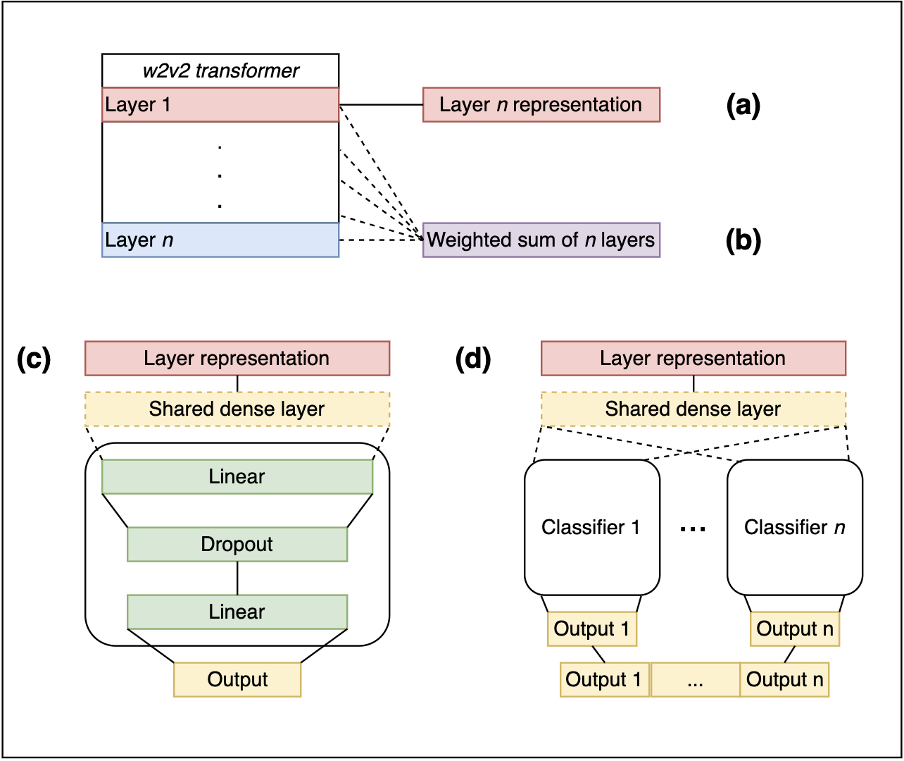
Figure 1: Architecture of our models. (a) shows how a single layer representation is extracted from the base wav2vec 2.0 transformer. (b) shows a learnable weighted sum representation, where weights are learned for each layer representation to sum all layers into one representation. (c) shows the basic single classifier architecture, with an optional shared dense layer. (d) shows the multiple classifier head set up, with an optional shared dense layer.

As part of our experiments, we implemented the following classifier architecture options:

1. One classifier head to predict all pathological features (Figure 1c) vs. Separate classifier heads for each feature (Figure 1d). In the single classifier head setup, the final output size 5x1. In the separate classifier heads setup, each classifier outputs a 1x1 prediction, which are concatenated into a 5x1 vector. This contrast of classifiers was motivated by the fact that each predicted pathological feature differs in domain of impairment (i.e., prosody, respiratory-phonatory, articulation [10]), such that learning to classify all features could potentially cause interference. Additionally, if there is a large difference in performance across features, then there may not be one best layer. Leveraging this would require multiple classifiers.

2. An additional shared dense layer with ReLU activation and an optional bottleneck parameter, added prior to the classification head(s) (Figure 1c-d), to see if sharing information between classifier heads improves performance.

3. An optional learnable weighted sum, added immediately after the transformer block , which takes speech representations from all transformer layers (Figure 1b) [12]. This method is less computationally costly than searching for a best layer.

Toolkits. Our model was implemented with PyTorch [19], using a pre-trained wav2vec 2.0 base [17] model and various functions from HuggingFace [18].

Training. Recordings were processed by resampling to 16 kHz and converting to mono channel. Each run was fine-tuned on 1 GPU, with 8 recordings per batch for 20 epochs. We used the AdamW [20] optimizer and binary cross entropy loss (BCEWithLogitsLoss). No warm-up or learning rate scheduler was used. For reproducibility, we used a fixed manual seed of 4200 across all runs. The base single classifier configuration had 594,437 trainable parameters while the base multi-classifier configuration had 2,956,805 trainable parameters. Adding a shared dense layer added an additional 590,592 trainable parameters, and adding a learnable weighted sum added only 13 parameters (one for each layer in the model). In total, each model configuration had between 95M and 98M parameters.

Hyperparameter and architecture tuning. We conducted a grid search with the following parameters: learning rate (1e-4, 1e-3), weight decay (1e-4, 1e-3, 1e-2), dropout probability (0.2, 0.3), classifier bottleneck (None, 700, 300), shared dense layer bottleneck (None, 700, 300). This search was run multiple times with different numbers of classifiers (1,5), inclusion/exclusion of shared dense layer, speech representations extracted from different model layers (1-13), and learnable weighted sum. Of these parameters, only learning rate had a visible impact on performance. As such, we fixed the following parameters: weight decay = 1e-4, dropout probability = 0.3, classifier bottleneck = None, shared dense layer bottleneck = None. We then ran another grid search only considering learning rate (1e-4, 1e-3) and layer (1-13, weighted sum) across all different classifier configurations for more direct comparison between hyperparameter tuning and layer selection.

Evaluation. We calculated the balanced accuracy to evaluate the models. These metrics account for imbalance in the target classes. We additionally conducted bootstrap sampling of the predictions (n=1000) to calculate the 95

4 Results

4.1 Hyperparameter tuning

We found that for our models, the only hyperparameter that impacted performance was the learning rate, with a learning rate of 0.001 offering comparable or slightly better performance on the best layer for almost all features, but this difference was small compared to the effect of layer selection (Figure 2). The difference in performance in terms of balanced accuracy across the best and worst layers averaged at 16.5% (min: $lr=0.0001$, irregular artic breakdowns, 5.5%; max: $lr=0.001$, strained, 22.5%) while the difference in performance across learning rate averaged at 2.4% (min: worst layer, rapid rate, 0%; max: worst layer, irregular artic breakdowns, 6.7%) These trends held for all model configurations.

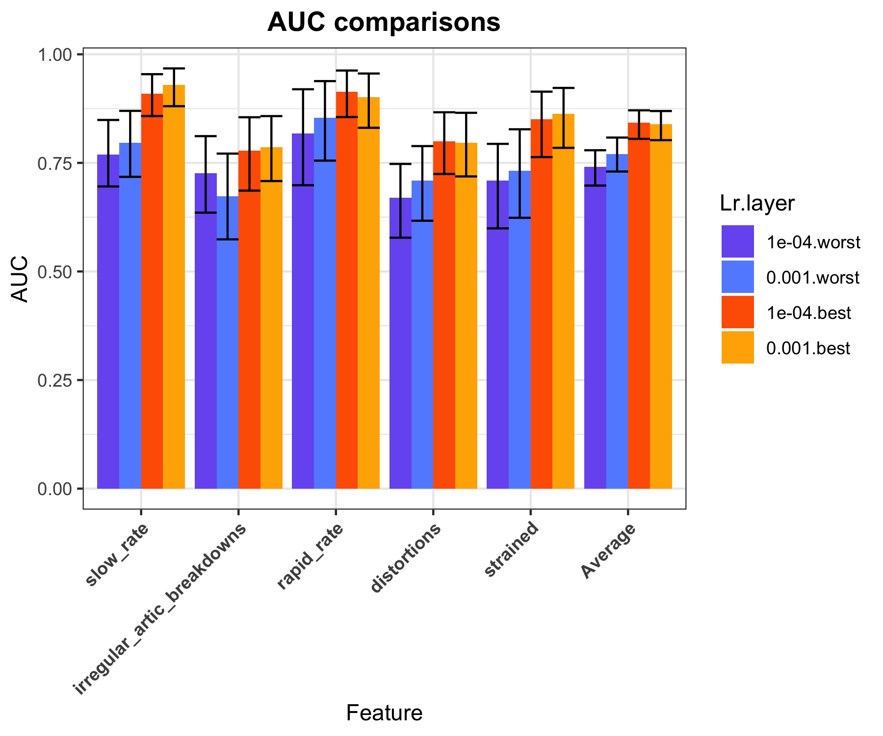
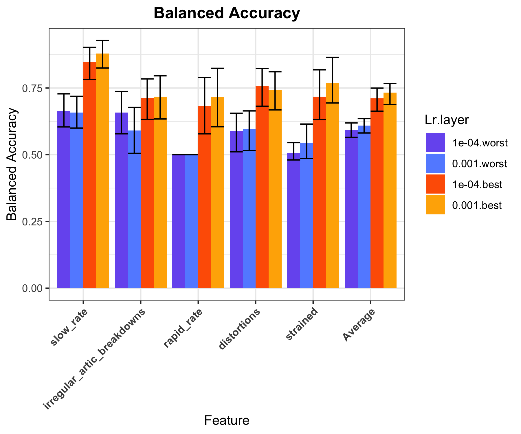
Figure 2: Comparing metrics by learning rate and layer across the predicted pathological speech features. These plot shows the (1) AUC and (2) balanced accuracy results from models with a single classifier and no shared dense layer or learnable weighted sum. The models were trained and tested with AMR recordings.

4.2 Classifier architecture

Table 2: AUC (averaged across features) for each classifier configuration and layer. Bold indicates best performing layer.

Layer	5, sd	5, No sd	1, No sd	1, sd
0	0.74	0.77	0.78	0.75
1	0.79	0.80	0.82	0.79
2	0.80	0.80	0.81	0.79
3	0.81	0.81	0.83	0.82
4	0.82	0.82	0.83	0.82
5	0.81	0.83	0.84	0.82
6	0.80	0.82	0.83	0.80
7	0.79	0.81	0.81	0.80
8	0.77	0.79	0.80	0.78
9	0.77	0.80	0.80	0.77
10	0.79	0.80	0.80	0.78
11	0.80	0.79	0.79	0.80
12	0.79	0.76	0.78	0.78
Weighted Sum	0.81	0.83	0.83	0.81

Table 3: Balanced accuracy (averaged across features) for each classifier configuration and layer. Bold indicates best performing layer.

Layer	5, sd	5, No sd	1, No sd	1, sd
0	0.66	0.69	0.69	0.67
1	0.68	0.68	0.71	0.70
2	0.68	0.69	0.69	0.69
3	0.71	0.70	0.72	0.69
4	0.70	0.69	0.70	0.69
5	0.68	0.67	0.71	0.69
6	0.68	0.68	0.72	0.68
7	0.66	0.70	0.67	0.67
8	0.65	0.68	0.69	0.66
9	0.67	0.68	0.69	0.67
10	0.65	0.69	0.68	0.66
11	0.65	0.66	0.63	0.62
12	0.60	0.61	0.61	0.60
Weighted Sum	0.69	0.69	0.70	0.68

Changes in classifier architecture also had minimal impact on performance as compared to layer, with differences in balanced accuracy across architectures averaging to 3.1% per layer, while difference across layers averaged to 10.25% per configuration (Table 3). In general, the early to middle layers of the wav2vec 2.0 model offered much better performance across all classifier architectures. The final layer of the model was consistently the worst, an important point considering the most common approach when transfer learning with this model is to use the final layer of hidden states. Notably, the learned weighted sum of layers offered performance comparable to the best layers (within 2%) while adding very few trainable parameters.

In general, the single classifier had slightly better performance (72% vs. 70% for the best layer(s)), and the addition of the shared dense layer never improved performance. The single classifier with no additional shared dense layer had the fewest trainable parameters of all configurations, meaning the difference in performance is not simply due to having more learnable parameters.

When looking closer at the impact of layer selection on performance for each predicted feature, we again saw that performance tended to peak in earlier or middle layers, with worst performance often at the final layer, and that a single classifier still generally offered better performance than multiple classifiers (Figure 3). Each feature did vary in terms of overall performance and in terms of the exact best layer (e.g., distortions peaked in layer 2 while slow rate peaked in layer 5) regardless of the classifier architecture. As a result, the average best layer was not always the best layer for any given feature. The learnable weighted sum was not as comparable to the best layers, though it still surpassed the worst layer by a large margin for all features (Figure 3, 4). It was much more comparable to the best layer when averaging across features, with a balanced accuracy of 70.1% as compared to the best layer (3) 71.6%.

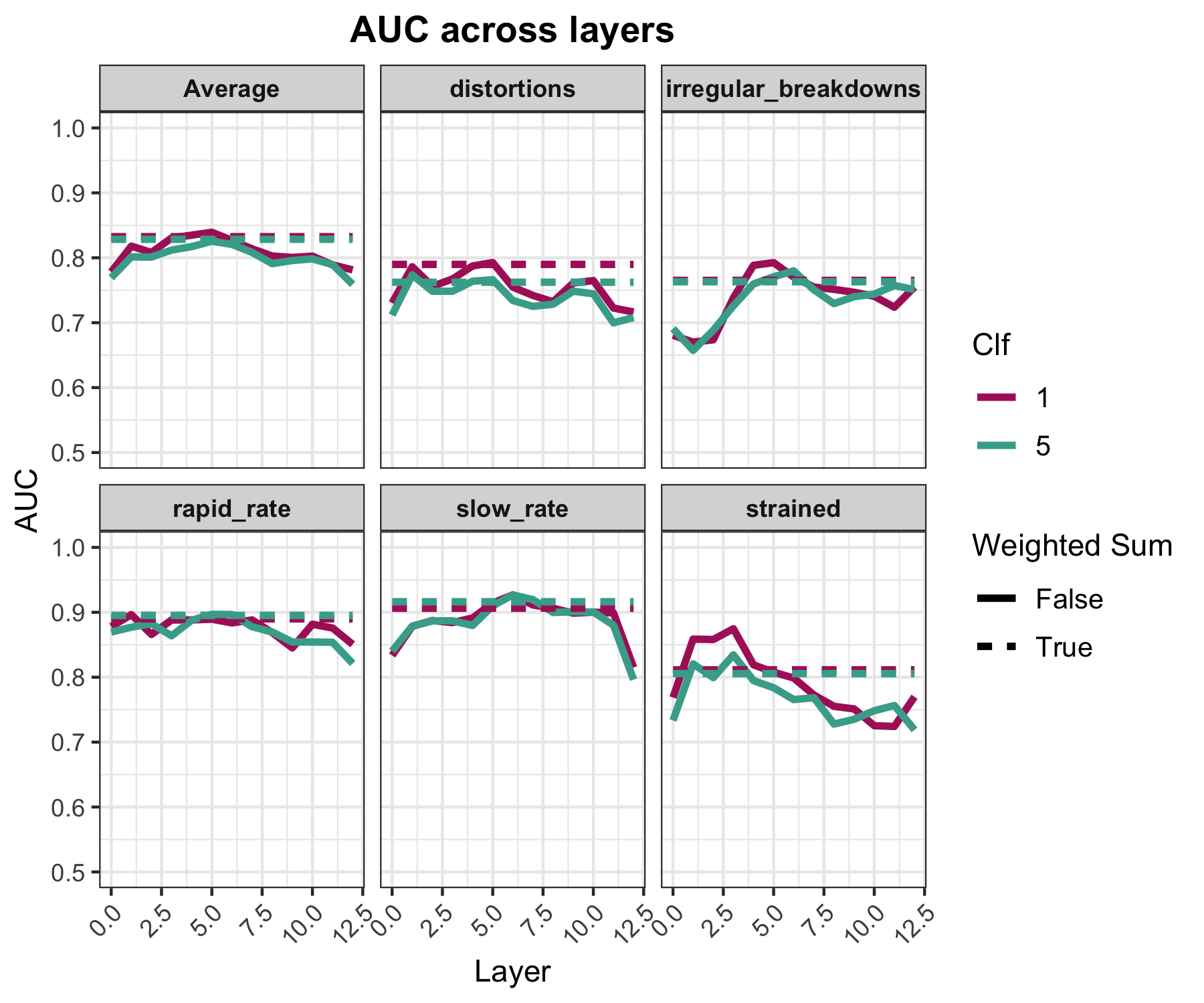
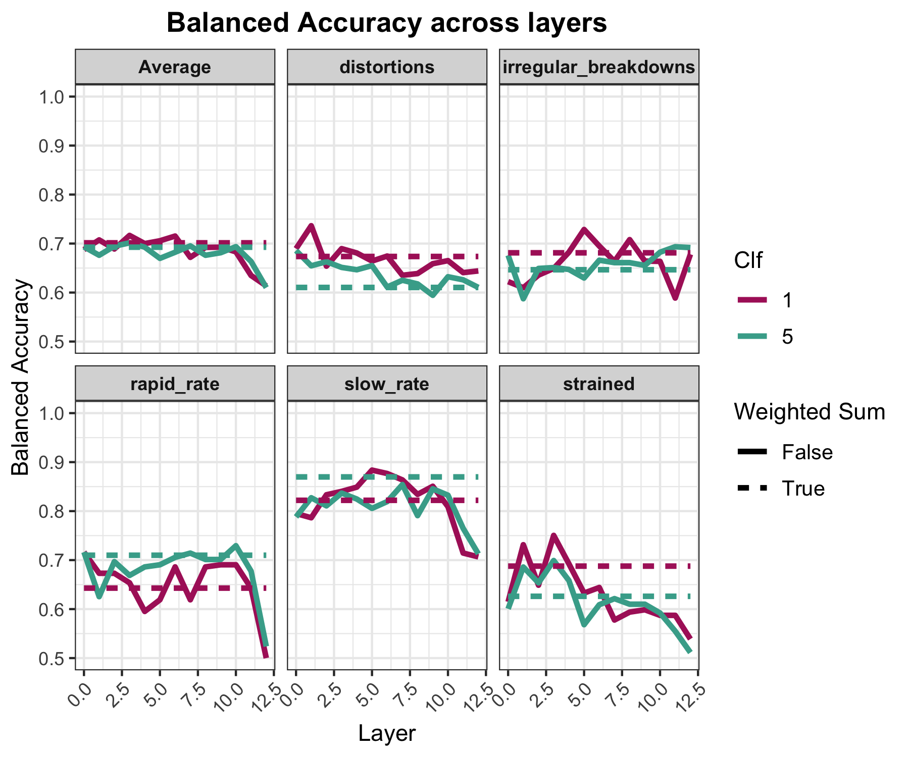
Figure 3: Comparing metrics by number of classifiers, layer, and weighted sum across the predicted pathological speech features. These plots show the (1) AUC and (2) balanced accuracy results from models trained and tested with AMR recordings. The model configurations do not include a shared dense layer and use a learning rate of 0.001.

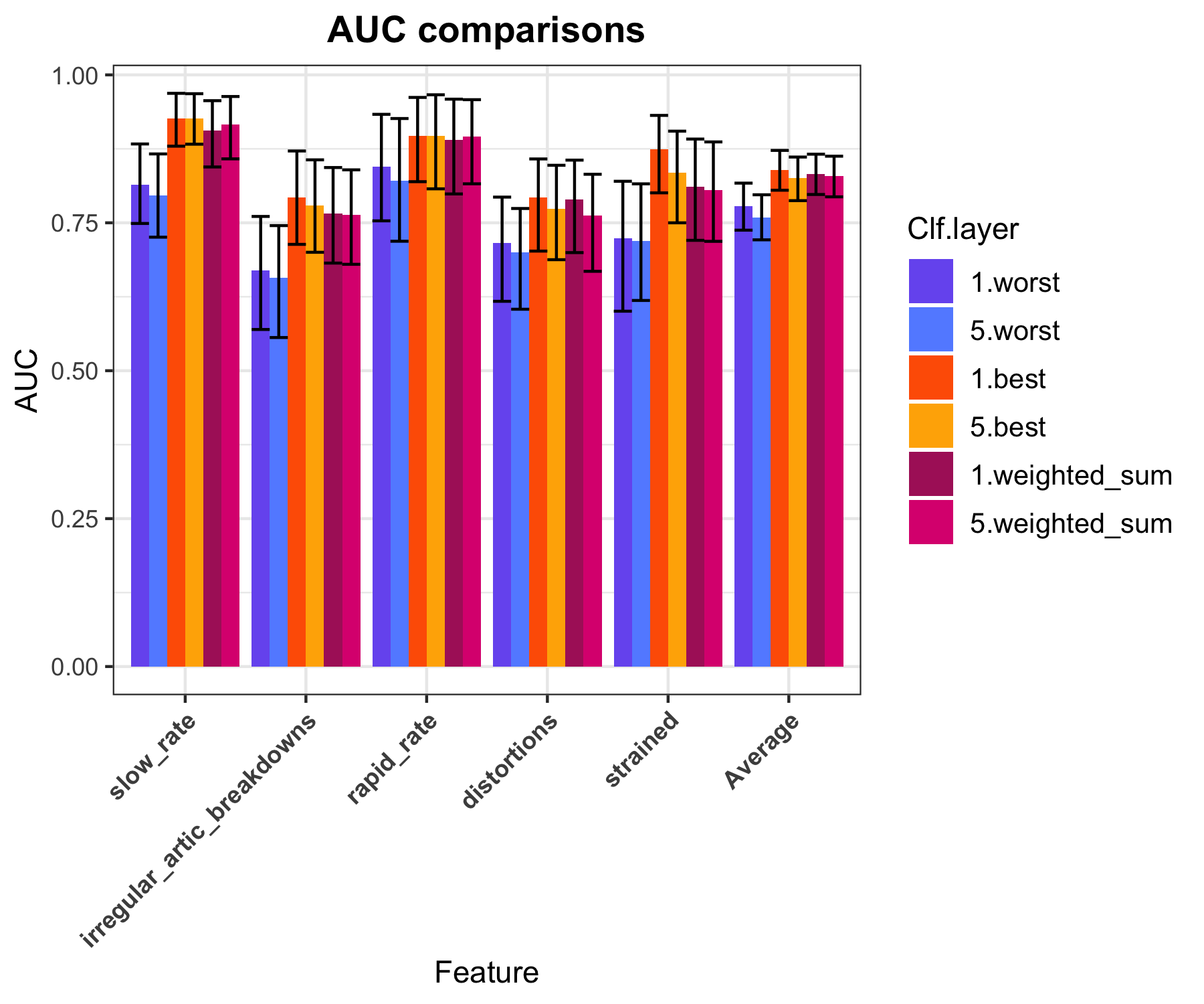
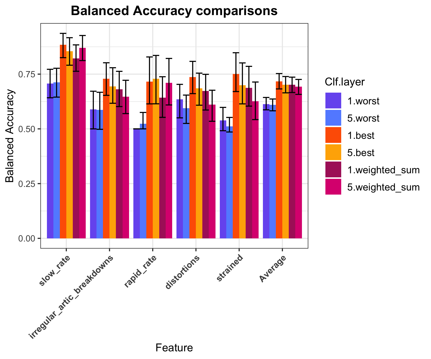
Figure 4: Comparing metrics by number of classifiers, best and worst layer, and learned weighted sum across the predicted pathological speech features. These plots show the (1) AUC and (2) balanced accuracy results from models trained and tested with AMR recordings. The model configurations do not include a shared dense layer and use a learning rate of 0.001.

4.3 Generalizability

To examine the generalizability of models optimized by layer selection, we generated predictions on an out-of-distribution test set of SMR recordings. Performance was worse for the out-of-distribution cases, but layer choice did seem to have some influence on generalizability (Figure 5). We no longer see a trend of performance peaking in middle layers, but on average, earlier layers still performed better than later layers. This was not the case for every feature, with distortions and irregular articulatory breakdowns showing later peaks, though never peaking on the last layer. The weighted sum offered the best, or near best, performance in the out-of-distribution tests.

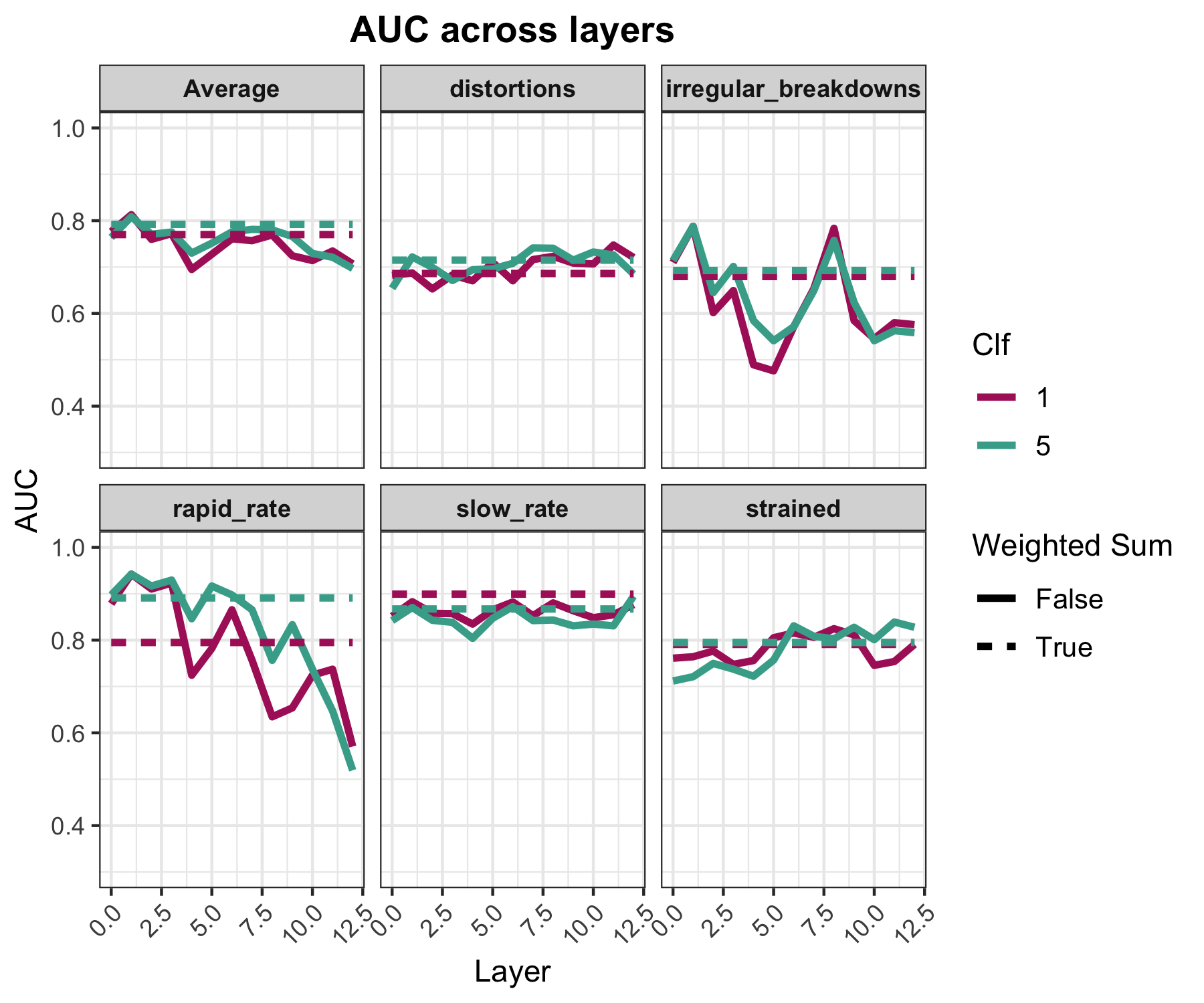
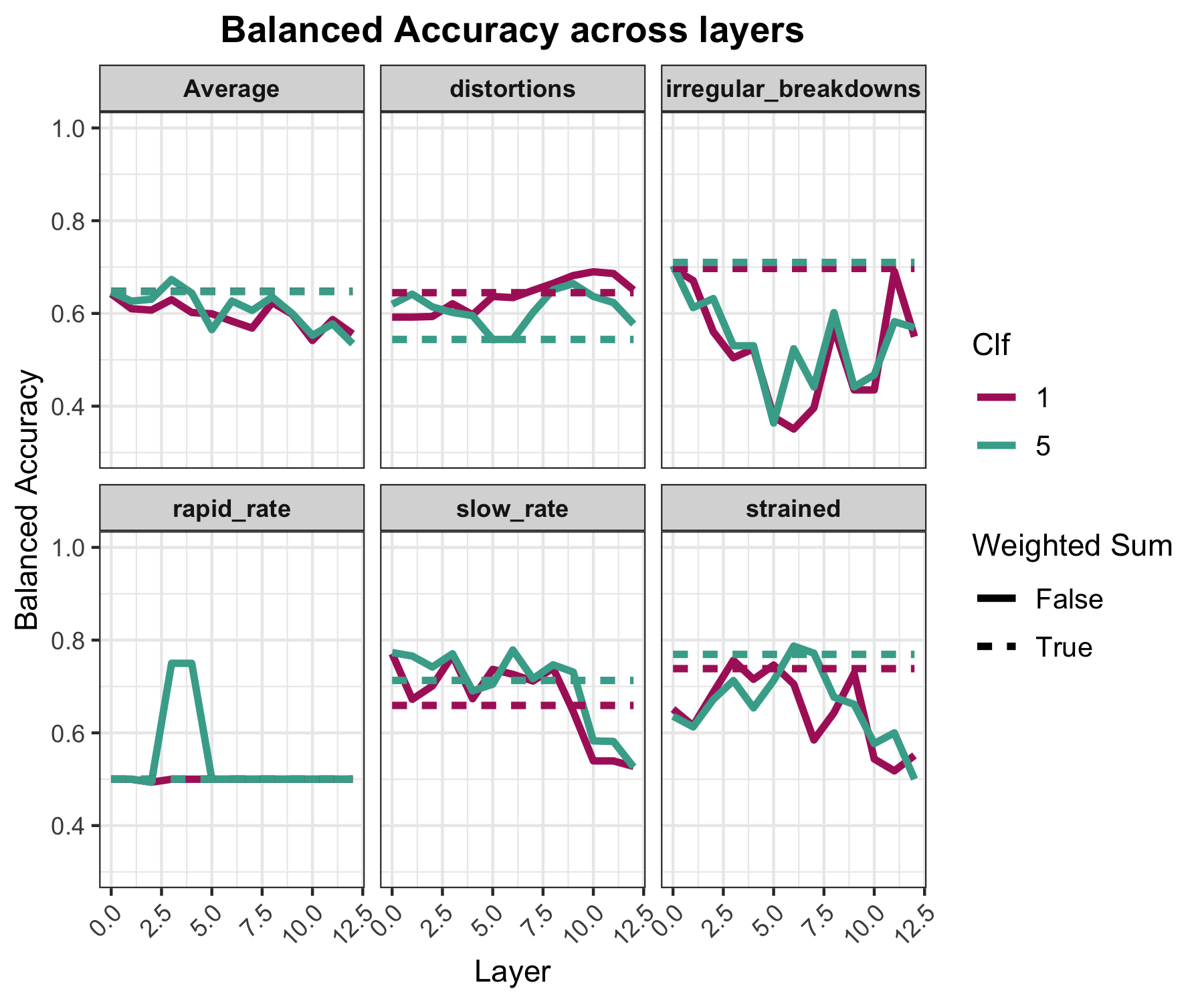
Figure 5: Comparing metrics by number of classifiers, layer, and weighted sum across the predicted pathological speech features. These plots shows the (1) AUC and (2) balanced accuracy results from models trained with AMR recordings and tested with SMR recordings (out-of-distribution). The model configurations do not include a shared dense layer and use a learning rate of 0.001.

5 Discussion

Our results showed that when attempting to make use of pre-existing pre-trained speech models for the clinical task of pathological speech prediction, layer selection plays the biggest role in improving model performance. Selecting the best layer improved the balanced accuracy by an average of 12.4%, with an improvement of up to 20% for certain features. This improvement was much larger than that of hyper-parameter tuning ($\sim 2\%$) or changes to the classifier architecture ($\sim 3\%$). However, the best layer was not consistent across features, though it tended to be earlier to middle layers in the model. On average, adding a learnable weighted sum to combine all layer representations offered comparable performance to the best performing layer, or at least improved upon using the final layer of the model.

The trend across layers for each feature was not the same in the out-of-distribution test. The best layers in the in-distribution test were rarely the best for the out-of-distribution test, showing that selecting only the best layers may not generalize well. On the other hand, the learnable weighted sum did have higher performance for out-of-distribution recordings than any single layer when considering the average balanced accuracy. This may suggest that optimizing based on single layer selection has an increased risk of overfitting. In a clinical setting, this is important to recognize as there are frequent out-of-distribution cases, both in terms of the form of the speech (a variety of elicited speech tasks) and the pathological features present in the speech.

This trend is likely because different intermediate representations capture different information about speech, with some representations being better suited for clinical tasks [12, 16]. The difference in best layer across feature follows from this, as pathological speech features have varied influence on a speech signal [10]. As a result, it is understandable that no single layer captures all the relevant information, such that average performance is often lower than that of the best performance per feature. Additionally, other aspects of the speech signal connected to the recording task or dataset demographics may be easier to encode in certain representations, leading to the best layers being dataset specific. The learnable weighted sum may be a valuable tool to increase generalization as it offered comparable performance to the average best layer and maintained the performance better than any single layer in out-of-distribution tests. Future work may look to improve the weighted sum, potentially by replacing it with a small network that allows the final representation to take only the best parts of each layer, rather than weighting the entire layer.

In general, the models did not perform to an acceptable standard for clinical use, but there is still a limited amount of data to fine-tune models with. We may see further improvement based on the quality and quantity of data alone. As more data becomes available, differences in performance connected to classifier architecture may exhibit a different trend than seen in this study. The amount of data as compared to the number of parameters may have led to poor learning. With more data, it may be worthwhile to fine-tune the speech representation model, or at least some of the final layers of the model, along with the classifier. This was shown to offer improvement for downstream tasks not originally in the model objective [12]. Our dataset is also mostly made up of white, non-Hispanic, American speakers and most of the speakers are middle aged or older, so our findings may not generalize to other races, ethnicities, accents, or ages.

We did not explore why certain features had better performance than others in depth, nor did we explore having separate classifiers with separate layer selections (i.e. choosing the best layer per feature). Leveraging this knowledge may be useful for further optimization. Previous work also did find that different models store information in different places [12], though there is some evidence that choice of model has lower impact than model-internal optimization [9]. Even so, some pre-trained models may be more suited to extracting clinically relevant speech representations [16]. Exploring layer selection across a variety of pre-trained models may therefore be a relevant next step.

6 Conclusion

We found that layer selection offers large performance improvements when leveraging pre-trained speech models for the downstream clinical task of predicting pathological speech features. In general, an earlier or middle layer outperformed the final layer of the model, though the exact best layer varied by feature and was not the same for in-distribution and out-of-distribution cases. A learned weighted sum offered comparable performance to the average best layer in-distribution and had better generalization for out-of-distribution data. While the best layer performance was consistently higher, the generalization power of the learned weighted sum may be better suited for the demands of clinical tasks.

7 Data availability

Our datasets are not publicly available given the nature of the recordings. Since the dataset contains clinical speech sample, there is potential for patient re-identification and for accidental leaking of private health information (PHI). As such, the data is only available within our institution.

8 Code availability

The source code will be available at https://github.com/dwiepert/naip-w2v2.

References

- [1] J. Dang, J. Graff-Radford, J. R. Duffy, R. L. Utianski, H. Clark, J. Stierwalt, J. L. Whitwell, K. A. Josephs, and H. Botha, ``Progressive apraxia of speech: Delays to diagnosis and rates of alternative diagnoses,'' J. Neurol., vol. 268, no. 12, pp. 4752–4758, 2021.
- [2] E. R. Dorsey, B. P. George, B. Leff, and A. W. Willis, ``The coming crisis: obtaining care for the growing burden of neurodegenerative conditions.'' Neurology, vol. 80, no. 21, pp. 1989–1996, 2013.
- [3] T. Koch, S. Iliffe, and the EVIDEM-ED project, ``Rapid appraisal of barriers to the diagnosis and management of patients with dementia in primary care: a systematic review.'' BMC Fam. Practice., vol. 11, p. 52, 2010.
- [4] R. Gupta, T. Chaspari, J. Kim, N. Kumar, D. Bone, and S. Narayanan, ``Pathological speech processing: State-of-the-art, current challenges, and future directions,'' in 2016 IEEE International Conference on Acoustics, Speech and Signal Processing (ICASSP), 2016, pp. 6470–6474.
- [5] J. P. Cohen, T. Cao, J. D. Viviano, C.-W. Huang, M. Frolic, M. Ghassemi, M. Madani, R. Greiner, and Y. Bengio, ``Problems in the deployment of machine-learned models in health care,'' Canadian Medical Association Journal, vol. 193, no. 35, pp. E1391–E1394, 2021.
- [6] H. Christensen, S. Cunningham, C. Fox, P. Green, and T. Hain, ``A comparative study of adaptive, automatic recognition of disordered speech,'' in Proc. Interspeech 2012, 2012, pp. 1776–1779.
- [7] D. Le, K. Licata, and E. Mower Provost, ``Automatic quantitative analysis of spontaneous aphasic speech,'' Speech Communication, vol. 100, pp. 1–12, 2018.
- [8] A. Tripathi, S. Bhosale, and S. K. Kopparapu, ``Automatic speaker independent dysarthric speech intelligibility assessment system,'' Computer Speech & Language, vol. 69, p. 101213, 2021. [Online]. Available: https://www.sciencedirect.com/science/article/pii/S0885230821000206
- [9] H. Soltau, I. Shafran, A. Ottenwess, J. R. Duffy, R. L. Utianski, L. R. Barnard, J. L. Stricker, D. Wiepert, D. T. Jones, and H. Botha, ``Detecting speech abnormalities with a perceiver-based sequence classifier that leverages a universal speech model,'' in 2023 IEEE Automatic Speech Recognition and Understanding Workshop (ASRU), 2023.
- [10] J. Duffy, Motor Speech Disorders E-Book: Substrates, Differential Diagnosis, and Management. Elsevier Health Sciences, 2019. [Online]. Available: https://books.google.com/books?id=O8q1DwAAQBAJ
- [11] A. Pasad, J.-C. Chou, and K. Livescu, ``Layer-wise analysis of a self-supervised speech representation model,'' in 2021 IEEE Automatic Speech Recognition and Understanding Workshop (ASRU), 2021, pp. 914–921.
- [12] A. Pasad, B. Shi, and K. Livescu, ``Comparative layer-wise analysis of self-supervised speech models,'' in ICASSP 2023 - 2023 IEEE International Conference on Acoustics, Speech and Signal Processing (ICASSP), 2023, pp. 1–5.
- [13] S. A. Chowdhury, N. Durrani, and A. Ali, ``What do end-to-end speech models learn about speaker, language and channel information? a layer-wise and neuron-level analysis,'' Computer Speech & Language, vol. 83, p. 101539, 2024.
- [14] F. Bertini, D. Allevi, G. Lutero, D. Montesi, and L. Calzà, ``Automatic speech classifier for mild cognitive impairment and early dementia,'' ACM Transactions on Computing for Healthcare, vol. 3, no. 1, 2021. [Online]. Available: https://doi.org/10.1145/3469089
- [15] C. Quan, K. Ren, Z. Luo, Z. Chen, and Y. Ling, ``End-to-end deep learning approach for parkinson's disease detection from speech signals,'' Biocybernetics and Biomedical Engineering, vol. 42, no. 2, pp. 556–574, 2022. [Online]. Available: https://www.sciencedirect.com/science/article/pii/S0208521622000341
- [16] D. Wagner, I. Baumann, F. Braun, S. P. Bayerl, E. Nöth, K. Riedhammer, and T. Bocklet, ``Multi-class detection of pathological speech with latent features: How does it perform on unseen data?'' 2023.
- [17] A. Baevski, H. Zhou, A. Mohamed, and M. Auli, ``Wav2vec 2.0: A framework for self-supervised learning of speech representations,'' in Proceedings of the 34th International Conference on Neural Information Processing Systems, ser. NIPS'20. Red Hook, NY, USA: Curran Associates Inc., 2020.
- [18] T. Wolf, L. Debut, V. Sanh, J. Chaumond, C. Delangue, A. Moi, P. Cistac, T. Rault, R. Louf, M. Funtowicz, J. Davison, S. Shleifer, P. von Platen, C. Ma, Y. Jernite, J. Plu, C. Xu, T. L. Scao, S. Gugger, M. Drame, Q. Lhoest, and A. M. Rush, ``Huggingface's transformers: State-of-the-art natural language processing,'' 2020.
- [19] A. Paszke, S. Gross, F. Massa, A. Lerer, J. Bradbury, G. Chanan, T. Killeen, Z. Lin, N. Gimelshein, L. Antiga, A. Desmaison, A. Kopf, E. Yang, Z. DeVito, M. Raison, A. Tejani, S. Chilamkurthy, B. Steiner, L. Fang, J. Bai, and S. Chintala, ``Pytorch: An imperative style, high-performance deep learning library,'' in Advances in Neural Information Processing Systems 32. Curran Associates, Inc., 2019, pp. 8024–8035. [Online]. Available: http://papers.neurips.cc/paper/9015-pytorch-an-imperative-style-high-performance-deep-learning-library.pdf
- [20] I. Loshchilov and F. Hutter, ``Decoupled weight decay regularization,'' 2019.