kNN Algorithm for Conditional Mean and Variance Estimation with Automated Uncertainty Quantification and Variable Selection

Abstract

In this paper, we introduce a kNN-based regression method that synergizes the scalability and adaptability of traditional non-parametric kNN models with a novel variable selection technique. This method focuses on accurately estimating the conditional mean and variance of random response variables, thereby effectively characterizing conditional distributions across diverse scenarios.Our approach incorporates a robust uncertainty quantification mechanism, leveraging our prior estimation work on conditional mean and variance. The employment of kNN ensures scalable computational efficiency in predicting intervals and statistical accuracy in line with optimal non-parametric rates. Additionally, we introduce a new kNN semi-parametric algorithm for estimating ROC curves, accounting for covariates. For selecting the smoothing parameter k, we propose an algorithm with theoretical guarantees.Incorporation of variable selection enhances the performance of the method significantly over conventional kNN techniques in various modeling tasks. We validate the approach through simulations in low, moderate, and high-dimensional covariate spaces. The algorithm’s effectiveness is particularly notable in biomedical applications as demonstrated in two case studies. Concluding with a theoretical analysis, we highlight the consistency and convergence rate of our method over traditional kNN models, particularly when the underlying regression model takes values in a low-dimensional space.

1   Introduction

Regression analysis [Györfi et al., 2002] is central to both statistics and machine learning. It typically involves predictors, denoted as $X$, within a $p$-dimensional space $\mathcal{X}=\mathbb{R}^{p}$, and a real-valued response variable $Y$ in $\mathbb{R}$. Traditionally, statistical research has focused on estimating the regression mean function $m(x)=\mathbb{E}(Y\mid X=x)$ [Kneib et al., 2023]. This estimation process is pivotal in developing new regression algorithms and applying them to diverse scientific problems. However, an exclusive focus on the conditional mean $m$, while neglecting the broader conditional distribution relationship between $Y$ and $X$, can lead to an incomplete understanding of the underlying phenomenon [Kneib et al., 2023, Klein, 2024].

From a statistical learning perspective, non-parametric estimation of the conditional distributional function

$$F(t,x)=\mathbb{P}(Y\leq t|X=x),$$

for each $t\in\mathbb{R}$ and $x\in\mathbb{R}^{p}$ is challenging [Hall et al., 1999, Klein, 2024]. Traditional methods, such as the Nadaraya-Watson estimator [Devroye, 1978] and local polynomial regression [Fan, 2018], are significantly affected by the curse of dimensionality [Collomb, 1981] and require smoothed conditions. Current literature and practitioners often lean towards parametric models, using linear quantile regression models [Koenker, 2005, Beyerlein, 2014] or recent distributional regression approaches, like the generalized additive model for location, scale, and shape [Rigby and Stasinopoulos, 2005] (GAMLSS) family as proxies. In other settings, such as survival analysis and the study of censored variables, the focus shifts to specific semi-parametric models [Kosorok, 2008] like Cox proportional hazards [Cox, 1972] and accelerated failure time models [Barnwal et al., 2022].

A compromise between non-parametric models and simpler models, such as linear homoscedastic quantile regression [Mu and He, 2007], is offered by scale-location models (see for example [Akritas and Van Keilegom, 2001, Zhao and Yang, 2023]). These models assume the following functional form for the regression model:

$$Y=m(X)+\epsilon\sigma(X),$$ (1)

where $\epsilon$ is a random error satisfying structural conditions such as $\mathbb{E}(\epsilon)=0$ and $X\perp\epsilon$ or $\epsilon\sim\mathcal{N}(0,1)$. These conditions are necessary to identify the conditional distribution with the knowledge of functions $m(\cdot)$ and $\sigma(\cdot)$, which represent the regression functions of location and scale, respectively.

This paper focuses on models represented by the above equation but from the perspective of the k-nearest neighbors (kNN) algorithm [Fix and Hodges, 1989, Stone, 1977, Biau and Devroye, 2015]. We propose new estimators to estimate the functions $m(\cdot)=\mathbb{E}(Y\mid X=\cdot)$ and $\sigma^{2}(\cdot)=\text{Var}(Y\mid X=\cdot)$. These models are designed to scale in large applications and achieve fast convergence rate, especially when the underlying regression models are defined in a low-dimensional manifold structure [Kpotufe, 2011, Vural and Guillemot, 2018].

We propose a straightforward yet effective multiple data-splitting strategy, specifically engineered to bypass post-selection [Chernozhukov et al., 2015] biases in various stages of model development. This approach is further enhanced by innovative variable selection methods [Guyon and Elisseeff, 2003, Bertsimas et al., 2020] meticulously adapted for both mean and variance regression functions. The goal is to significantly improve model scalability and model inference, and to expedite convergence rate.

Furthermore, we establish mathematical criteria for determining the smoothing parameters in the kNN algorithm, a crucial step in enhancing the accuracy of our regression function approximations (see a discussion here [Zhao and Lai, 2021]). Within the framework of our semi-parametric kNN approach, we introduce two novel algorithms: i) Algorithm designed to derive robust prediction intervals [Gyôrfi and Walk, 2019]; ii) algorithm specialized in estimating Receiver Operating Characteristic curves (ROC) [Cai and Pepe, 2002], particularly in scenarios involving covariates.

1.1 Summary of Contributions

This paper presents a new kNN-based predictive framework, advancing beyond conventional kNN regression methods in estimating mean and variance regression functions, $m(\cdot)$ and $\sigma^{2}(\cdot)$. Our approach integrates an innovative variable selection strategy, which significantly enhancer model convergence rates. The key contributions are:

1. Efficient and Interpretable Estimation:

   • Scalability: The employment of the nearest neighbor algorithm, as elucidated by [Andoni et al., 2019], facilitates scalability in large-scale applications, offering a robust framework for handling extensive datasets. Moreover, subsequent methodologies that evolve from this algorithm exhibit quasilinear complexity.

   • Variable Selection and Interpretability: Our variable selection method improves model interpretability, elucidating the impact of key variables on the mean and variance of the response variable.

   • Theoretical Guarantees: Due to variable selection step, the proposal offers enhanced convergence in low-dimensional manifold representations of the regression model [Kpotufe, 2011].

   • Adaptive Tuning Parameter Selection: Introduces a data-driven rule for optimal selection of the $k$-parameters [Azadkia, 2019], thereby improving mean and variance estimation accuracy.

   • Conditional Distribution Recovery: Effectively recovers the conditional distribution in various scale and localization models [Akritas and Van Keilegom, 2001], surpassing traditional non-parametric local conditional distributional methods [Dombry et al., 2023], particularly in homoscedastic contexts [Goldfeld and Quandt, 1965].

2. Prediction Interval Estimation: We propose a new suite of prediction intervals for scale-localization models, yielding competitive results compared to non-parametric methods [Gyôrfi and Walk, 2019] with added computational efficiency.

3. ROC Analysis in Presence of Covariates: Our method facilitates the estimation of conditional ROC curves [Cai and Pepe, 2002], crucial in medical research for the validation of new therapeutical biomarkers [Kulasingam and Diamandis, 2008]. We demonstrate its effectiveness in validating biomarkers for screening diabetes mellitus.

4. Biomedical Applications: This section underscores the significant impact and broad relevance of our models in biomedical research, particularly highlighting their potential for use in large-scale medical studies. The models are distinctively non-parametric, marking a major shift from the traditional parametric methods [Su et al., 2018] commonly used in the creation of clinical prediction scores.

1.2 Outline

This paper is structured as follows. Section 3 introduces the mathematical models, including regression estimators, variable selection, prediction interval analysis, and ROC methods. Section 4 discusses the theoretical aspects, focusing on consistency checks, convergence rates, and the $k$-rule optimality. Section 5 presents a comprehensive simulation analysis, highlighting strengths and addressing limitations for a well-rounded understanding of our model. In Section 6, we apply our model to a large-scale real-world problem, showcasing its practical relevance in biomedical contexts. The paper concludes with Section 7 summarizing key findings and future research directions.

2   Background and related work

The kNN algorithm, foundational to non-parametric regression, was theoretically established by [Cover and Hart, 1967, Stone, 1977] and practically introduced by [Fix and Hodges, 1989]. Noted for its simplicity and adaptability, kNN’s effectiveness spans various predictive tasks [Yong et al., 2009, Chen et al., 2018, Li et al., 2021]. Unlike smoothers like Nadaraya-Watson, kNN does not rely on strict smoothing assumptions, a significant advantage in real-world applications [Fan, 2018, Gyôrfi and Walk, 2019].

kNN operates effectively with both independent and dependent data [Biau et al., 2010], addressing continuous and discrete responses [Zhang et al., 2017], and managing complex scenarios like censored variables [Chen, 2019] and counterfactual inference [Zhou and Kosorok, 2017]. It has shown efficacy in clustering large datasets [Shi et al., 2018], uncertainty quantification [Gyôrfi and Walk, 2019], functional data analysis [Kara et al., 2017], and metric space modeling [Györfi and Weiss, 2021, Cohen and Kontorovich, 2022]. Theoretical contributions include advancements in adaptive manifold methods [Kpotufe, 2011, Jiang, 2019], minimax estimators [Zhao and Lai, 2021], and non-parametric conditional entropy estimation [Kozachenko and Leonenko, 1987, Berrett et al., 2019].

In terms of distributional convergence [Biau and Devroye, 2015] and empirical process analysis [Portier, 2021], kNN has been notable. Convergence rates under conditions like Lipchitz in the regression function are well established [Györfi et al., 2002], with modified conditions explored for optimal prediction intervals [Gyôrfi and Walk, 2019].

While the primary focus in statistical modeling has been on conditional mean estimation, recent advancements have turned towards conditional variance estimation, particularly in low-dimensional spaces. This shift was initially spurred by the development of Conditional U-statistics, as introduced by Stute [Stute, 1991] and furthered by various two-step methods (see for example [Müller and Stadtmüller, 1993, Padilla, 2022]). Additionally, in the realm of conditional distribution estimation [Dombry et al., 2023], kNN models have not been extensively explored within a semi-parametric framework [Kosorok, 2008], which is a key aspect of our proposal. Our methods also uniquely incorporate variable selection and optimal tuning of smoothing parameters.

In the current landscape, neural networks and deep learning algorithms [Bartlett et al., 2021] undoubtedly dominate real-world applications, especially in the context of non-parametric regression and massive-data environments, with a particular focus on conditional mean estimation. The use of neural networks (NNs) for estimating conditional distributions has primarily been explored in the field of survival analysis (see for example [Rindt et al., 2022, Meixide et al., 2022]). However, in various scenarios, kNN methods can offer a viable alternative to neural network models. For instance, NNs encounter considerable challenges in model inference, especially when employing bootstrap methods [Härdle and Bowman, 1988] and asymptotic approximations. Their tendency to settle into local minima can significantly undermine the reliability of inference, an issue that becomes more pronounced in complex models. This problem is particularly acute in bootstrap methods, where the inherent stochasticity of NNs leads to inconsistent convergence of estimators. Furthermore, NNs are prone to overfitting in high-dimensional data, a risk that is amplified when dealing with bootstrap’s resampled datasets. The lack of interpretability and the substantial computational demands of NNs further limit their applicability in specific scenarios, such as real-time or resource-constrained environments. This is notably evident in the context of smartphone and wearable data used in research and clinical settings.

3   Mathematical Methods

In practice, we observe a random sample $\mathcal{D}_{n}=\{(X_{i},Y_{i})\}_{i=1}^{n}$, comprising independent and identically distributed (i.i.d.) samples from the joint distribution of $(X,Y)\in\mathcal{X}\times\mathcal{Y}$. Here, $\mathcal{X}=\mathbb{R}^{p}$ and $\mathcal{Y}=\mathbb{R}$, with $X=(X^{1},\ldots,X^{p})$ being a $p$-dimensional absolutely continuous random variable. For analytical purposes, the dataset $\mathcal{D}_{n}$ is divided into four random subsets $\mathcal{D}_{j}$, indexed by $\mathcal{S}_{j}=\{i\in[n]:=\{1,\dots,n\}:(X_{i},Y_{i})\in\mathcal{D}_{j}\}$ for $j\in\{1,2,3,4\}$, such that $|\mathcal{S}_{j}|=n_{j}$.

Mathematical Population Framework

The objective of our study is to estimate two key regression functions within a fixed-effect framework. These functions are $m:\mathbb{R}^{p_{1}}\rightarrow\mathbb{R}$ and $\sigma:\mathbb{R}^{p_{2}}\rightarrow\mathbb{R}$, for the mean and standard deviation, respectively, where $p_{1}$ and $p_{2}$ denote the dimensions of the input spaces for each function. The model is specified as follows:

$$Y=m(X^{\text{mean}})+\epsilon\cdot\sigma(X^{\text{var}}),$$ (2)

where $\epsilon\sim\mathcal{N}(0,1)$ represents a normally distributed random error term. In this model, $X^{\text{mean}}=\{X^{j}:j\in A\}$ and $X^{\text{var}}=\{X^{j}:j\in B\}$ signify subsets of the input variables that influence the conditional mean and variance, respectively. The sets $A$$\subset[p]=\{1,\dots,p\}$ and $B$ $\subset[p]$ can represent different sources of information in the data. The inclusion of the term $\epsilon\sim\mathcal{N}(0,1)$ allows us to capture the conditional distribution of $Y$ given $X$ as follows:

$$F(t,x) =\mathbb{P}(Y\leq t\mid X=x)$$ (3)

$$=\mathbb{P}\left(\epsilon\leq\frac{t-m(X^{\text{mean}})}{\sigma(X^{\text{var}})}\mid X=x\right),$$ (4)

where $F(t,x)$ denotes the cumulative distribution function (cdf).

Definition 3.1.

(Homoscedastic scale-localization model) The model defined in Eq. 2 is said to be homoscedastic if the function $\sigma$ is a constant (i.e., $\sigma=c$ where $c>0$ is an arbitrary constant). In contrast, if $\sigma(\cdot)$ is not constant, the model is said to be heteroscedastic, indicating a variance that changes with the input $X$.

Prediction Interval definition: Prediction intervals are crucial tools to understand the uncertainty of predictions and establish the reliability of data-driven approaches. For a new observation $(X_{n+1},Y_{n+1})$, the oracle population prediction interval is defined as the interval with minimum length. Setting the confidence level $\alpha\in(0,1)$ and assuming that $\epsilon$ is a symmetrical random error, the prediction interval (assuming it exist and is unique) is given by:

$$C^{\alpha}(X_{n+1})=\bigg{[}m(X_{n+1}^{\text{mean}})-c_{\alpha}\sigma(X_{n+1}^{\text{var}}),\\ m(X_{n+1}^{\text{mean}})+c_{\alpha}\sigma(X_{n+1}^{\text{var}})\bigg{]},$$

where $c_{\alpha}$ satisfies $\mathbb{P}(Y_{n+1}\in C^{\alpha}(X_{n+1})\mid X_{n+1})=1-\alpha$.

ROC Analysis problem:

In our study, we introduce a novel approach to Receiver Operating Characteristic (ROC) analysis, termed semi-parametric ROC analysis, based on the conditional distributional model outlined in Eq. 3. This method focuses on a continuous biomarker, denoted as $Y$, and a covariate $X$, enhancing ROC curve analysis by incorporating covariates.

Traditional ROC curves, used extensively in medical and diagnostic testing [Nakas et al., 2023], plot the True Positive Rate (TPR) against the False Positive Rate (FPR) across various thresholds. However, these standard analyses do not account for covariates that might influence test performance. Our approach addresses this limitation.

We define the conditional cumulative distribution functions (cdf’s) of $Y$ for individuals with disease ($D$) and without disease ($H$), given the covariate $X=x$, as $F_{D|X}(y,x)$ and $F_{H|X}(y,x)$, respectively. This enables the computation of TPR and FPR at threshold $c$ for a given covariate $x$:

$$\text{TPR}(c|x) =1-F_{D|X}(c,x),$$

$$\text{FPR}(c|x) =1-F_{H|X}(c,x).$$

These conditional rates facilitate plotting a ROC curve for each $x$ value, providing a more detailed view of the test’s performance. Moreover, we compute the Area Under the Curve (AUC) for each covariate value $x$ as:

$$\text{AUC}(x)=\int_{0}^{1}\text{TPR}(\text{FPR}^{-1}(u)|X=x)|X=x)du,$$

where $\text{FPR}^{-1}(u|X=x)$ is the inverse function of FPR for a given covariate value $x$.

3.1 Conditional Mean Estimation via kNN Regression

For clarity, we will focus on defining the estimator using a single random sample, denoted $\mathcal{D}_{n}$ and its subsamples $\mathcal{D}_{j}\subset\mathcal{D}_{n}$, where $j\in\{1,2,3,4\}.$

The kNN regression algorithm is one of the earliest non-parametric methods for estimating the conditional mean. It is known for its scalability and strong theoretical properties, which are generally more robust than other regression methods, such as Nadaraya-Watson, that require smoothness [Györfi et al., 2002]. Given a positive integer $k_{1}:=k_{\text{mean}}>0$, which represents the number of points used to estimate the local mean at an arbitrary point $x\in\mathcal{X}$, and a norm $\left\lVert\mkern 2.0mu\cdot-\cdot\mkern 2.0mu\right\rVert$, we arrange the elements of the random sample $\mathcal{D}_{n}$ in ascending order of their distance to $x$. Specifically, $X_{(1:n)}(x),\ldots,X_{(n:n)}(x)$ are arranged such that $\left\lVert\mkern 2.0mux-X_{(1:n)}(x)\mkern 2.0mu\right\rVert\leq\cdots\leq\left\lVert\mkern 2.0mux-X_{(n:n)}(x)\mkern 2.0mu\right\rVert$. The neighborhood $N_{k_{1}}(x)$ is then defined as $N_{k_{1}}(x):=N_{k_{1}}(x):=\left\{i\in[n]:\left\lVert\mkern 2.0mux-X_{i}\mkern 2.0mu\right\rVert\leq\left\lVert\mkern 2.0mux-X_{(k_{1}:n)}(x)\mkern 2.0mu\right\rVert\right\}$.

The basic estimator for the conditional mean function $m$ is expressed as

$$\widehat{m}_{k_{1},n}(x)=\frac{1}{k_{1}}\sum_{i\in N_{k_{1}}(x)}Y_{i},$$

with a local sample mean around the random elements indexed by $N_{k_{1}}(x)$. Under our data-splitting strategy, we can use this algorithm on a random subsample, $\mathcal{D}_{j}$, for $j\in\{1,2,3,4\}$. For each data point in $\mathcal{D}_{j}$, we define

$$N_{k_{1}}^{\mathcal{D}_{j}}(x):=\{i\in\mathcal{S}_{j}:\lVert x-X_{i}\rVert\leq\lVert x-X_{(k_{1}:n_{j})(x)}\rVert\}$$

where $X_{(k:n_{j})}(x)$ denotes the $k$-th nearest neighbor in $\mathcal{D}_{j}$. The refined estimator is then given by

$$\widehat{m}_{k_{1},n_{j}}(x)=\frac{1}{k_{1}}\sum_{i\in N_{k_{1}}^{\mathcal{D}_{j}}(x)}Y_{i}.$$

3.2 Conditional Variance Estimation via Residuals

To estimate the conditional variance, we employ a two-step method based on the prior estimate $\widehat{m}_{k_{1},n_{j-1}}$, for $j\geq 2$. Given a fixed $k_{2}:=k_{\text{var}}>0$, we first define the residuals for each $i\in\mathcal{S}_{j}$ as:

$$\widehat{\epsilon}_{i}=Y_{i}-\widehat{m}_{k_{1},n_{j-1}}(X_{i}).$$

Here, $\widehat{m}_{k_{1},n_{j-1}}(\cdot)$ is typically estimated using $\mathcal{D}_{j-1}$, which under structural hypotheses is i.i.d. from $\mathcal{D}_{j}$. Using these residuals, we model $\widehat{\epsilon_{i}}^{2}$ as the random response variable:

$$\widehat{\sigma}_{k_{2},n_{j}}^{2}(x)=\frac{1}{k_{2}}\sum_{i\in N_{k_{2}}^{\mathcal{D}_{j}}(x)}\widehat{\epsilon}_{i}^{2}.$$

The conditional variance $\sigma^{2}(x)$ is defined as:

$$\text{Var}(Y|X =x)=\mathbb{E}\left[(Y-m(x))^{2}|X=x\right]=\mathbb{E}[\epsilon^{2}|X=x]$$

This formulation implies that if the first regression function $\widehat{m}_{k_{1},n_{j-1}}(\cdot)$ is consistent, then the estimator for the variance $\sigma^{2}(\cdot)$, denoted as $\widehat{\sigma}_{k_{2},n_{j}}^{2}(\cdot)$, will also be consistent under traditional kNN mean regression conditions (see [Stone, 1977, Györfi et al., 2002]) as $n_{j-1}\to\infty$ and $n_{j}\to\infty$.

3.3 General Variable Selection strategy for kNN

The proposed methods are grounded in the principles of explainable machine learning, drawing inspiration from the findings presented in two key papers [Lei et al., 2018, Verdinelli and Wasserman, 2021].

Given the two-step nature of our estimator $\sigma(\cdot)$, which depends on the mean function $m(\cdot)$, our exposition primarily elucidates the variable selection algorithm for $m$. The approach for $\sigma$ mirrors that for $m$, albeit applied independently on a different dataset.

Consider the regression function $m(\cdot)$ and $m_{-j}(\cdot)$, the latter obtained by excluding the $j$-th variable. We assess the $j$-th predictor’s significance via $W(X,Y)=\left\lVert\mkern 2.0muY-m_{-j}(X)\mkern 2.0mu\right\rVert^{2}-\left\lVert\mkern 2.0muY-m(X)\mkern 2.0mu\right\rVert^{2}$, where $\left\lVert\mkern 2.0mu\cdot\mkern 2.0mu\right\rVert$ denotes the squared Euclidean distance. For each predictor $j$, we define the integrated measure $w_{j}=\mathbb{E}[\left\lVert\mkern 2.0muY-m_{-j}(X)\mkern 2.0mu\right\rVert^{2}]-\mathbb{E}[\left\lVert\mkern 2.0muY-m(X)\mkern 2.0mu\right\rVert^{2}]$.

Theoretically, under the null hypothesis $H_{0}$: the $j$-th predictor, among $\{1,\ldots,p\}$, is irrelevant if $W(X,Y)$ is zero almost surely. For each predictor $j$, within $\{1,\ldots,p\}$, we employ a formal hypothesis testing framework. Define $\widetilde{W}_{j}(x,y)=\left\lVert\mkern 2.0mu(y-\widehat{m}_{-j,k_{1},n_{l}}(x))\mkern 2.0mu\right\rVert^{2}-\left\lVert\mkern 2.0muy-\widehat{m}_{k_{1},n_{l}}(x)\mkern 2.0mu\right\rVert^{2}$ and consider the mean over a separate random split $\mathcal{D}_{l}$. We compute $\widetilde{w}_{j}=\frac{1}{n_{l}}\sum_{i\in\mathcal{D}_{l}}\widetilde{W}_{j}(X_{i},Y_{i})$ and evaluate the null hypothesis $H_{0}:w_{j}\leq 0$ against $H_{a}:w_{j}>0$ using for example a t-test.

Our proposal includes an asymptotically sound rule adapted to the kNN algorithm, ensuring universal consistency. Alternatively, traditional hypothesis testing statistics, such as a paired test, can be used, circumventing the need for regression estimators in the mean function. For a rate improvement, in some cases, we advocate a resampling bootstrap approach, like double bootstrap (for variance step), to better calibrate the test, accounting for variations in estimating the functions $m$ and $\sigma$, respectively. In all cases, errors diminish as the sample size grows, thereby improving hypothesis testing calibration. Considering the application of these methods in large-scale datasets, the kNN-bias associated with test statistics is not a practical concern. By evaluating $\widetilde{w}_{j}$ on another data splitting, we minimize this issue and limit the correlation problem between relevant and non-relevant variables, as mentioned in [Verdinelli and Wasserman, 2021]. The use of a specific $k$-rule in the variable selection algorithm also minimizes this bias, as it adapts the estimators to the underlying smoothness of the true regression function.

From a practical perspective, a Bonferroni correction is implemented to adjust for the simultaneous statistical significance testing across potentially $p$-mean and $p$-variance variables.

Remark 3.2.

The recent algorithm proposed by [Györfi et al., 2023] builds upon their earlier work [Devroye et al., 2018] on conditional mean and variance selection. This development closely aligns with our hypothesis testing approach. However, our methodology distinctly focuses on the conditional mean and variance. Furthermore, we approach the variable selection problem as a series of $2\times p$ multiple testing problems, each centered on univariate hypothesis testing. This contrasts with the global strategy in [Györfi et al., 2023], which does not perform a different data-splitting for the $k$-rule selection.

While our approach may introduce additional multiple-testing problems, as noted in [Brzyski et al., 2017], it compensates with enhanced statistical power, especially when compared to the method presented in [Devroye et al., 2018]. This advantage becomes particularly pronounced in cases where $p\geq 2$. For further insights into the power of local non-parametric tests under general alternatives, refer to the discussions in [Janssen, 2000, Ramdas et al., 2015].

3.4 Optimal $k$-Parameter Selection

Building upon the advancements in $k$-parameter selection for conditional means as discussed in [Györfi et al., 2002, Azadkia, 2019], we propose a streamlined leave-out-cross-validation rule for selecting the $k$-parameter for both mean and variance functions that provide strong-non asymptotic guarantees. Specifically, we define $\widetilde{k}$ as follows:

$$\widetilde{k}:=\operatorname{argmin}_{1\leq k\leq n-1}f(k),$$ (5)

where $f(k)$ is given by

$$f(k):=\frac{1}{n}\sum_{i=1}^{n}\left(Y_{i}-\frac{1}{k}\sum_{j\in N_{k}(X_{i})}Y_{j}\right)^{2}.$$

3.5 Data Splitting Strategy

To enhance the efficiency and scalability of our model, we implement variable selection and $k$-selection in distinct data splits at each step of the modeling process. Fig. 1 illustrates the critical components and algorithmic details. Specifically, within additional data splits, denoted as $\mathcal{D}_{j}\subset\mathcal{D}_{n}$ where $j\geq 5$, we conduct further modeling tasks. These tasks leverage the strengths of our semi-parametric algorithm, as elaborated below. This structured approach to data handling and model building not only streamlines the process but also ensures robust and scalable performance across diverse datasets.

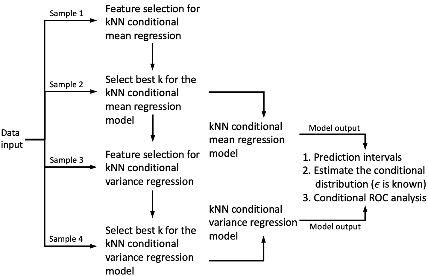
Figure 1: Model-data splitting strategy and extensions in the kNN semi-parametric framework.

3.6 Model Extensions: Predictive Interval Algorithm

In the development of predictive models, accurately quantifying uncertainty is paramount for ensuring both reliability and trustworthiness of data-driven methods. Traditional methods, such as conformal prediction [Shafer and Vovk, 2008, Barber et al., 2023], bootstrap Dimitris–Politis framework [Zhang and Politis, 2023], and Bayesian methods each offer specific advantages and limitations. These include dependence on the exchangeability hypothesis in the case of conformal prediction, computational efficiency issues in bootstrapping in large-scale applications, and reliance on the accuracy of underlying parameterized models, especially in Bayesian methods. Recently, Gyorfi et al. [Gyôrfi and Walk, 2019] introduced an alternative scalable kNN-based method that provides optimal non-parametric prediction intervals under minimal conditions. This paper builds on that work by proposing enhanced new algorithm kNN variant, more effective in homoscedastic contexts. We introduce two distinct approaches: a fully non-parametric version and a more efficient semi-parametric version. Both focus on estimating the mean function $m(\cdot)$ and the standard deviation function $\sigma(\cdot)$.

Semi-Parametric Prediction

In three independent data splits, denoted as $\mathcal{D}_{j-2}$, $\mathcal{D}_{j-1}$, and $\mathcal{D}_{j}$ (for $j\geq 3$), we obtain the estimators: i) $\widehat{m}_{k_{1},n_{j-2}}(\cdot)$, ii) $\widehat{\sigma}_{k_{2},n_{j-1}}(\cdot)$. In step iii), for all $i\in\mathcal{S}_{j}$, we define the standardized residuals

$$\widehat{\epsilon}_{i}=\frac{Y_{i}-\widehat{m}_{k_{1},n_{j-2}}(X_{i})}{\widehat{\sigma}_{k_{2},n_{j-1}}(X_{i})}.$$

Furthermore, we define the empirical $(1-\alpha)$ quantile $\widehat{q}_{1-\alpha}$ based on the set of residuals $\{\widehat{\epsilon}_{i}\}_{i\in\mathcal{S}_{j}}$. For each $\alpha\in(0,1)$, we return the prediction interval

$$\widehat{C}^{\alpha}(x)=\bigg{[} \widehat{m}_{k_{1},n_{j-2}}(x)-\widehat{q}_{1-\alpha}\widehat{\sigma}_{k_{2},n_{j-1}}(x),$$

$$\widehat{m}_{k_{1},n_{j-2}}(x)+\widehat{q}_{1-\alpha}\widehat{\sigma}_{k_{2},n_{j-1}}(x)\bigg{]}.$$

Semi-Parametric Prediction

In the semi-parametric scenario, we adhere to steps i) and ii). However, for the calibration of the quantile $\widehat{q}_{1-\alpha}$, we leverage the assumption that the random error $\epsilon$ follows a normal distribution, specifically $\epsilon\sim\mathcal{N}(0,1)$. This approach pragmatically addresses potential errors arising from quantile estimation. Under ideal conditions of differentiability of the cumulative distribution function of the random error $\epsilon$, we can obtain the optimal parametric rate $\mathcal{O}_{p}(\frac{1}{\sqrt{n}})$ [Serfling, 2009]. In other i.i.d. settings, this rate decays as $\mathcal{O}_{p}(\frac{\log(n)}{n})$ [Csorgo et al., 1986]. This is contingent on the absence of measurement errors in the estimation of the random functions $\widehat{m}(\cdot)$ and $\widehat{\sigma}(\cdot)$.

3.7 Model Extensions: ROC-kNN Algorithm

We exploit the advantages of the semi-parametric conditional distribution kNN algorithm, defined in Eq. 3, to propose a new algorithm for deriving the ROC curve [Nakas et al., 2023] in massive datasets. The ROC curve is a critical tool for evaluating the diagnostic performance of biomarkers [Pepe et al., 2008] or models, particularly in the presence of covariates [Cai and Pepe, 2002]. This approach is tailored to assess the efficacy of diagnostic tests across a range of covariate values.

The area under the ROC curve (AUC) quantifies the overall diagnostic effectiveness of the biomarker [Nakas et al., 2023]. Here, we specifically consider the impact of a covariate $X$. An AUC value of $0.5$ indicates no diagnostic power, while a value of one implies perfect discrimination.

Assuming the diseased population $Y_{D}$ and the healthy population $Y_{H}$ have corresponding continuous diagnostic variables and covariate vectors $X_{D}$ and $X_{H}$, we simplify the approach by assuming that these covariates are identical in both groups. For a data split $\mathcal{D}_{j}$, $j\geq 2$, we estimate regression functions for both groups $l\in\{H,D\}$, namely, mean $\widehat{m}^{l}_{k_{1},n_{j-1}}(\cdot)$ and standard deviation $\widehat{\sigma}^{l}_{k_{2},n_{j}}(\cdot)$, facilitating the estimation of $F_{l|X}(t,x)$, $l\in\{D,H\}$. This is particularly applicable when the random error, as defined in Eq. 3, follows $\epsilon\sim\mathcal{N}(0,1)$. As outlined in Section 3, we estimate the conditional ROC curve $ROC(x,\rho)$, for $\rho\in[0,1]$. We focus on the estimation of the AUC, which can be expressed as:

$$\widehat{\text{AUC}}(x)=\int_{0}^{1}\left[1-\widehat{F}_{H|X}\left(\widehat{F}^{-1}_{D|X}(1-\rho,x),x\right)\right]d\rho.$$

4   Theory

In this section, we investigate some theoretical aspects of our kNN method. The proofs of all these results are relegated to the Supplementary Material.

Theorem 4.1 (Consistence of the mean and variance regression functions).

Given $|Y|\leq L,$ and $\mathbb{E}(|Y^{2r}|)<\infty$ for some $r\geq 1$, the kNN split regression estimate for the mean $m(\cdot)$ and variance $\sigma(\cdot)$ functions is $L_{r}$-consistent $(r\geq 1)$, if $k_{1}\rightarrow\infty$, $k_{1}/n_{1}\rightarrow 0$, $k_{2}\rightarrow\infty$, and $k_{2}/n_{2}\rightarrow 0$. This implies:

$$\mathbb{E}\left[\left|\sigma(X)-\widehat{\sigma}_{k_{2},n_{2}}(X)\right|^{r}\right]\rightarrow 0,\mathbb{E}\left[\left|m(X)-\widehat{m}_{k_{1},n_{1}}(X)\right|^{r}\right]\rightarrow 0.$$

Remark 4.2.

This result extends Stone’s theorem [Stone, 1977] to variance estimation using a data-splitting strategy in our kNN framework. It is important to note that the only condition placed on the variables $X,Y$ is $\mathbb{E}(|Y^{2r}|)<\infty$, which does not impose restrictions on their distributions.

Theorem 4.3 (Rates of kNN Scale-Localization Gaussian Model).

Let $\epsilon\sim\mathcal{N}(0,1)$ as defined in Eq. (3). For a given $x\in\mathcal{X}$, the approximation error of the conditional distribution function using our kNN algorithm is represented by

$$\left|\widehat{F}(\cdot,x)-F(\cdot,x)\right|=\mathcal{O}_{p}\left(n^{-\sigma}\right),$$

where $\mathcal{O}_{p}\left(n^{-\sigma}\right)$ denotes the convergence rate of function $\sigma$ using the kNN algorithm. This rate includes the error in estimating the mean function $m$.

Remark 4.4.

Our approach combines variable selection with data splitting. If it correctly identifies the true supports $p_{1}$ and $p_{2}$, and they are much smaller than the total number of variables $p$, this leads to enhanced rate efficiency. Moreover, as [Jiang, 2019] suggests, if the data naturally resides in a low-dimensional manifold, the actual convergence rate might be governed by reduced dimensions $p^{\prime}_{1}<p_{1}$ and $p^{\prime}_{2}<p_{2}$. This lower rate, compared to that from the higher dimensions in the ambient space, improves the model’s efficiency.

Remark 4.5.

In analyzing the accuracy of recovering distribution functions, it’s crucial to distinguish between homoscedastic (where $p_{2}=0$) and heteroscedastic scenarios (where $p_{2}>0$). In the homoscedastic case, the rate mainly hinges on the regression function $m(\cdot)$. For example, if $m$ is $\alpha$-Hölder continuous, the rate is $\mathcal{O}_{p}\left(n^{\frac{-2\alpha}{2\alpha+p_{1}}}\right)$, typical for homoscedastic situations. In contrast, in the heteroscedastic case, the rate is influenced by the variance function $\sigma(\cdot)$.

Considering the special case where $p_{1}=0$ and $p_{2}=0$, indicating perfect detection of true variables and the optimal k-rule for neighbor number, we can estimate the variance with a naive estimator at an optimal parametric rate of $\mathcal{O}_{p}\left(\frac{1}{\sqrt{n}}\right)$, aligning with model selection criteria for variable selection and smoothing. While non-parametric conditional distribution models generally do not achieve these rates, our method does under specific conditions, such as when $\mathbb{E}(Y^{r})<\infty$ for $r\geq 6$. This is discussed in [Grams and Serfling, 1973], particularly regarding the rate of sample variance and sample mean

Theorem 4.6 (Universal Consistency of kNN Rule for Variable Selection).

For a fixed number of covariates $p$, consider the variable selection method outlined in Section 3.3. This method is universally consistent for the mean function $m(\cdot)$ and variance function $\sigma(\cdot)$ as $n_{1}\to\infty$ and $n_{2}\to\infty$, provided $k_{1}\to\infty$, $k_{2}\to\infty$, $\frac{k_{1}}{n_{1}}\to 0$, and $\frac{k_{2}}{n_{2}}\to 0$. If we select the optimal $k_{1}$, $k_{2}$, parameters in different data-splits, the rate of selecting the significance of the $j$-th variable is $\mathcal{O}_{p}\left(\sqrt{\frac{\log(n)}{n}}\right)$.

5   Simulation data

This section compares empirically our kNN method against the conventional kNN algorithm. The latter lacks a variable selection mechanism, using all variables. We examine this in three regimes: (a) low-dimensional (1-2 variables), (b) medium-dimensional (5 variables), and (c) high-dimensional (up to 10 variables), with $B=300$ simulation runs each.

For each simulation $b\in\{1,\ldots,B\}$, random samples $\{(X_{i},Y_{i})\}_{i=1}^{n}$ follow $Y_{i}=m(X_{i})+\sigma(X_{i})\epsilon_{i}$, where $\epsilon_{i}\sim\mathcal{N}(0,1)$ and $X_{i}\sim U[0,1]^{p}$.

Simulations vary in covariate dimensions and sample sizes. Mean squared errors (MSE) are calculated as detailed in the Appendix. Each simulation includes a test dataset of $n_{test}=5000$ observations for Monte Carlo integration. The generative models used are summarized in Table 1 in the study. The eleven scenarios are discussed, with detailed results in the Supplemental Material.

The main conclusions of the simulation study are summarized here:

• The effectiveness of variable selection methods in our new approach becomes more apparent as $p$ increases. While the support of the true variables for mean and variance remains constant, the error in traditional kNN is significantly higher, even with larger samples. This is mainly due to the lack of two additional data splits for variable selection in traditional methods.

• The selection of the $k$ parameter demonstrates robustness, as evidenced in examples where the mean function $m(X)=c$. In these cases, the error is minimized, and the method tends to select the maximum number of neighbors.

• Our method shows substantial gains in terms MSE for both mean and variance estimations. In certain instances, improvements in MSE can be as high as 200 percent. Despite the inclusion of a variable selection step, larger sample sizes are still required in extensive datasets to ensure the error approaches zero due to the non-parametric nature of our method.

Table 1: Simulation Scenarios in Diferent Regimes

Regime	#	$m(X)$	$\sigma(X)$	$p$
Low	1	$5\cdot X^{2}+5\cdot X^{3}$	1	{3, 10, 20, 25}
	2	0	$5\cdot X^{1}$
	3	$5\cdot X^{2}+5\cdot X^{3}$	$5\cdot X^{1}$
Mod.	4	$5\cdot\sum_{i=1}^{4}X^{i}$	1	{5, 10, 20, 50}
	5	0	$5\cdot\sum_{i=1}^{4}X^{i}$
	6	$5\cdot\sum_{i=1}^{3}X^{i}$	$5\cdot(X^{4}+X^{5})$
	7	$5\cdot\sum_{i=1}^{4}X^{i}$	$5\cdot\sum_{i=2}^{5}X^{i}$
Large	8	$5\cdot\sum_{i=1}^{8}X^{i}$	1	{10, 25, 50, 100}
	9	$5\cdot\sum_{i=1}^{6}X^{i}$	$5\cdot\sum_{i=8}^{10}X^{i}$

6   Real Data Example about diabetes in NHANES

This section highlights the clinical relevance of our models for large-scale medical research. For additional case studies and a comprehensive array of illustrative figures, refer to the Supplemental Material.

This study conducts a thorough analysis of the NHANES dataset, which includes 56,301 individuals from 2002 to 2018, to investigate the association between waist circumference and diabetes risk factors. The focus is on estimating the conditional mean and variance of waist circumference, taking into account variables such as gender, age, BMI, among others. These factors are employed to refine models for both diabetic and non-diabetic groups, assisting in the generation of ROC curves, based on the assumption of a Gaussian distribution.

The analysis reveals significant differences in the results of the three models – overall, male, and female – in identifying key variables that influence both mean and variance. A notable discovery is the contrast in variable importance between diabetic and non-diabetic groups. In diabetic groups, all variables significantly affect conditional variance, unlike in non-diabetic groups. For the conditional mean, BMI and weight emerge as consistently critical across all models, highlighting how waist circumference, as a measure of fat distribution, is intrinsically linked to overall body composition, profoundly influencing mean predictions.

Gender-specific variations in conditional variability are evident in non-diabetic populations, particularly in mean and female models. While the male model incorporates all variables, the female model is more selective, reflecting intrinsic gender-based differences.

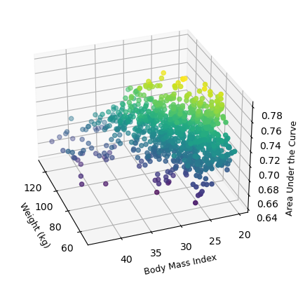
Figure 2: Three-dimensional scatter plot illustrating the area under the curve for weight and body mass index among male participants in the NHANES dataset.

This finding aligns with the ’Variability Hypothesis’ in human biology, which suggests that mean values hold more biological significance in several biological processes [Ju et al., 2015, Joel, 2021]. The importance of variable selection in enhancing the predictiveness and interpretability of models is emphasized, particularly in understanding scale and location effects in epidemiological research.

The ROC analysis for male participants (Fig. 2) demonstrates that the AUC for diabetes discrimination based on waist circumference biomarkers is remarkably high. This performance rivals that of traditional diabetes risk assessments that include a more comprehensive range of variables [Saaristo et al., 2005]. This finding stresses the need for personalized approaches in disease screening and the importance of developing tailored public health screening strategies, rather than relying solely on broad-based analyses.

7   Discussion and Conclusions

In this article, we have introduced a novel, quasi-optimal k-NN algorithm, featuring an innovative variable selection method for efficient approximation of conditional distributions in various settings. This algorithm operates under minimal conditions, making it theoretically robust. Its relevance is especially notable in modern clinical settings, where it has proven effective in handling extensive datasets. Notably, major medical studies, such as those involving the UK Biobank [Jenkins et al., 2024], now frequently encompass datasets with over 100,000 patients, demonstrating the increasing importance of such approaches.

Future developments of our algorithm will adapto the algorithm for local-variable selection following the paritions kernel methods outlined in [Rudi et al., 2017]. This advancement aims to provide localized variable selectors [Rossell et al., 2023] for precise mean and variance estimations across different subregions. We plan to further examine the algorithm’s ability to reconstruct conditional distribution functions, adjusting for random errors and various parametric distributions like beta-models. Comparative studies with techniques such as GAMLSS will be key to highlighting our approach’s unique advantages in large-scale applications

Simulation section

Simulation details

Our simulations span various covariate dimensions $p\in\{3,5,10,20,25,30,40,50,70,80,100,150,200\}$ and sample sizes $n\in\{5000,10000,20000,50000,100000\}$. We also consider different forms for $m(\cdot)$ and $\sigma(\cdot)$. For each simulation run $b$, we estimate the conditional mean and standard deviation as $\widehat{m}^{b}(\cdot)$ and $\widehat{\sigma}^{b}(\cdot)$, respectively. The mean squared metrics for these function estimations are defined as:

$$\widehat{MSS}^{m}=\frac{1}{B}\sum_{b=1}^{B}\int_{[0,1]^{p}}\left[\widehat{m}^{b}(x)-m(x)\right]^{2}\,\mu(dx),$$

and

$$\widehat{MSS}^{\sigma}=\frac{1}{B}\sum_{b=1}^{B}\int_{[0,1]^{p}}\left[\widehat{\sigma}^{b}(x)-\sigma(x)\right]^{2}\,\\ \ \mu(dx).$$

For computational feasibility in these metrics, each simulation $b$ includes an additional test dataset $\mathcal{D}_{\text{testsim}}$, generated under the same distribution as $(X,Y)$ and comprising $5000$ data points. This facilitates the approximation of integral calculations via Monte Carlo integration.

.1 Scenario $1$

		$p=3$		$p=10$		$p=20$		$p=25$
	$N$	$\overline{x}$	$\hat{v}$	$\overline{x}$	$\hat{v}$	$\overline{x}$	$\hat{v}$	$\overline{x}$	$\hat{v}$
FS	5000	0.0434	0.0206	0.0427	0.0117	0.0428	0.0110	0.0421	0.0157
	10000	0.0277	0.0242	0.0283	0.0091	0.0280	0.0064	0.0283	0.0105
	20000	0.0169	0.0022	0.0171	0.0021	0.0168	0.0024	0.0169	0.0021
	50000	0.0096	0.0015	0.0096	0.0015	0.0094	0.0013	0.0096	0.0014
	100000	0.0066	0.0012	0.0066	0.0012	0.0066	0.0012	0.0067	0.0012
No FS	5000	0.0947	0.0222	0.6488	0.3708	1.2960	1.4762	1.5220	2.1521
	10000	0.0618	0.0090	0.5156	0.2165	1.1232	1.1237	1.3434	1.6418
	20000	0.0405	0.0033	0.4117	0.1316	0.9711	0.8011	1.1863	1.2404
	50000	0.0245	0.0019	0.3116	0.0683	0.8116	0.4928	1.0158	0.8055
	100000	0.0173	0.0015	0.2568	0.0460	0.7094	0.3606	0.9080	0.6098

Table 2: Performance evaluations in scenario 1 (low regime) of the estimators $\overline{x}$ and $\hat{v}$ for the different k-NN graph settings described in the text with and without feature selection. We report the mean squared error averaging over 300 Monte Carlo simulations.

.2 Scenario $2$

		$p=3$		$p=10$		$p=20$		$p=25$
	$N$	$\overline{x}$	$\hat{v}$	$\overline{x}$	$\hat{v}$	$\overline{x}$	$\hat{v}$	$\overline{x}$	$\hat{v}$
FS	5000	0.0063	0.8026	0.0069	0.6997	0.0061	0.9310	0.0053	1.1172
	10000	0.0031	0.9373	0.0025	0.6875	0.0032	0.7145	0.0035	0.8270
	20000	0.0022	0.5057	0.0025	0.5198	0.0023	0.5029	0.0019	0.5409
	50000	0.0091	0.0595	0.0049	0.0556	0.0032	0.0550	0.0082	0.0604
	100000	0.0072	0.0214	0.0064	0.0202	0.0033	0.0206	nan	nan
No FS	5000	0.0081	1.0415	0.0063	1.4483	0.0066	1.6663	0.0054	1.7433
	10000	0.0036	2.1614	0.0037	1.3894	0.0032	1.6022	0.0033	1.7349
	20000	0.0022	0.8711	0.0023	1.2565	0.0020	1.4818	0.0020	1.5915
	50000	0.0017	0.3060	0.0015	0.8244	0.0015	1.1483	0.0016	1.2290
	100000	0.0013	0.1470	0.0014	0.6393	0.0014	0.9694	0.0014	1.0606

Table 3: Performance evaluations in scenario 2 (low regime) of the estimators $\overline{x}$ and $\hat{v}$ for the different k-NN graph settings described in the text with and without feature selection. We report the mean squared error averaging over 300 Monte Carlo simulations.

.3 Scenario $3$

		$p=3$		$p=10$		$p=20$		$p=25$
	$N$	$\overline{x}$	$\hat{v}$	$\overline{x}$	$\hat{v}$	$\overline{x}$	$\hat{v}$	$\overline{x}$	$\hat{v}$
FS	5000	0.0782	0.5546	0.0770	0.7934	0.0741	0.9381	0.0743	0.8808
	10000	0.0473	0.6874	0.0482	0.6662	0.0448	0.4978	0.0476	0.7247
	20000	0.0313	0.4962	0.0316	0.4151	0.0312	0.5146	0.0310	0.5302
	50000	0.0179	0.0583	0.0184	0.0526	0.0167	0.0653	0.0171	0.0519
	100000	0.0109	0.0191	0.0114	0.0193	0.0110	0.0180	0.0113	0.0211
No FS	5000	0.1437	1.0584	0.7315	1.9104	1.3806	3.3652	1.6027	4.0641
	10000	0.0932	2.2468	0.5888	1.6454	1.1959	3.0601	1.4157	3.3767
	20000	0.0643	0.8605	0.4889	1.4443	1.0455	2.4025	1.2613	3.0328
	50000	0.0398	0.3016	0.3688	0.9132	0.8894	1.7339	1.0935	2.1656
	100000	0.0261	0.1461	0.2963	0.6846	0.7799	1.3983	0.9801	1.7551

Table 4: Performance evaluations in scenario 3 (low regime) of the estimators $\overline{x}$ and $\hat{v}$ for the different k-NN graph settings described in the text with and without feature selection. We report the mean squared error averaging over 300 Monte Carlo simulations.

.4 Scenario $4$

		$p=5$		$p=10$		$p=20$		$p=50$
	$N$	$\overline{x}$	$\hat{v}$	$\overline{x}$	$\hat{v}$	$\overline{x}$	$\hat{v}$	$\overline{x}$	$\hat{v}$
FS	5000	0.1133	0.0217	0.1141	0.0230	0.1129	0.0347	0.1125	0.0383
	10000	0.0813	0.0192	0.0813	0.0110	0.0809	0.0226	0.0818	0.0135
	20000	0.0502	0.0042	0.0502	0.0042	0.0499	0.0046	0.0501	0.0044
	50000	0.0316	0.0022	0.0316	0.0023	0.0315	0.0023	0.0316	0.0025
	100000	0.0205	0.0015	0.0205	0.0015	0.0206	0.0016	0.0205	0.0016
No FS	5000	0.3144	0.0973	0.9331	0.7528	1.9036	3.1338	3.2565	9.9012
	10000	0.2196	0.0489	0.7475	0.4774	1.6510	2.3455	2.9914	8.2117
	20000	0.1609	0.0229	0.5931	0.2771	1.4356	1.7622	2.7798	7.1134
	50000	0.1095	0.0093	0.4424	0.1325	1.1936	1.0660	2.5235	5.4133
	100000	0.0776	0.0051	0.3594	0.0865	1.0426	0.7673	2.3573	4.5408

Table 5: Performance evaluations in scenario 4 (moderate regime) of the estimators $\overline{x}$ and $\hat{v}$ for the different k-NN graph settings described in the text with and without feature selection. We report the mean squared error averaging over 300 Monte Carlo simulations.

.5 Scenario $5$

		$p=5$		$p=10$		$p=20$		$p=50$
	$N$	$\overline{x}$	$\hat{v}$	$\overline{x}$	$\hat{v}$	$\overline{x}$	$\hat{v}$	$\overline{x}$	$\hat{v}$
FS	5000	0.0184	4.7813	0.0159	5.2681	0.0168	5.6835	0.0168	6.0965
	10000	0.0086	4.6833	0.0107	4.7571	0.0091	5.9863	0.0090	5.5643
	20000	0.0071	3.9487	0.0063	4.3996	0.0055	4.5909	0.0060	5.0149
	50000	0.0294	2.2449	0.0092	2.0947	0.0094	2.3559	0.0091	2.4721
	100000	0.0090	0.6105	0.0116	0.5900	0.0064	0.6193	0.0115	0.8261
No FS	5000	0.0173	4.6294	0.0159	5.1821	0.0167	5.6338	0.0169	6.0650
	10000	0.0082	4.0516	0.0106	4.5364	0.0085	5.9468	0.0090	5.5558
	20000	0.0059	3.2773	0.0063	4.0511	0.0055	4.6751	0.0059	5.3154
	50000	0.0045	1.6746	0.0043	2.6123	0.0045	3.5756	0.0044	4.5143
	100000	0.0041	1.0421	0.0042	1.9987	0.0039	2.9740	0.0041	4.0399

Table 6: Performance evaluations in scenario 5 (moderate regime) of the estimators $\overline{x}$ and $\hat{v}$ for the different k-NN graph settings described in the text with and without feature selection. We report the mean squared error averaging over 300 Monte Carlo simulations.

.6 Scenario $6$

		$p=5$		$p=10$		$p=20$		$p=50$
	$N$	$\overline{x}$	$\hat{v}$	$\overline{x}$	$\hat{v}$	$\overline{x}$	$\hat{v}$	$\overline{x}$	$\hat{v}$
FS	5000	0.1099	2.9097	0.1097	4.4237	0.1122	3.9644	0.1313	3.9069
	10000	0.0753	3.0066	0.0730	2.9182	0.0742	4.4914	0.0751	3.2367
	20000	0.0451	1.9320	0.0443	1.8292	0.0445	1.9821	0.0452	2.1602
	50000	0.0283	0.3856	0.0279	0.4115	0.0280	0.4079	0.0276	0.4491
	100000	0.0160	0.1599	0.0160	0.1600	0.0160	0.1666	0.0159	0.2308
No FS	5000	0.3938	2.7810	0.8619	3.7975	1.5102	5.7212	2.3795	14.4896
	10000	0.2765	2.6488	0.7041	3.1965	1.3164	5.0554	2.1878	8.8444
	20000	0.2127	2.1886	0.5547	2.8820	1.1492	4.2427	2.0193	7.2374
	50000	0.1378	1.0577	0.4186	1.8354	0.9508	3.0378	1.8181	5.8541
	100000	0.1062	0.6727	0.3475	1.3597	0.8323	2.4507	1.6972	5.0614

Table 7: Performance evaluations in scenario 6 (moderate regime) of the estimators $\overline{x}$ and $\hat{v}$ for the different k-NN graph settings described in the text with and without feature selection. We report the mean squared error averaging over 300 Monte Carlo simulations.

.7 Scenario $7$

		$p=5$		$p=10$		$p=20$		$p=50$
	$N$	$\overline{x}$	$\hat{v}$	$\overline{x}$	$\hat{v}$	$\overline{x}$	$\hat{v}$	$\overline{x}$	$\hat{v}$
FS	5000	0.4492	4.8810	0.4748	5.7071	0.5487	6.4132	0.8646	8.2382
	10000	0.2070	4.3001	0.2001	4.5830	0.2002	5.2007	0.2037	5.6938
	20000	0.1375	4.0639	0.1347	4.5087	0.1361	4.7070	0.1350	5.0836
	50000	0.0815	2.0606	0.0806	2.1841	0.0808	2.1381	0.0806	2.4248
	100000	0.0581	0.6724	0.0586	0.6185	0.0589	0.6884	0.0583	0.8257
No FS	5000	0.5957	4.8698	1.3052	6.4275	2.2609	11.2373	3.5751	17.7136
	10000	0.4200	3.9648	1.0572	5.7865	1.9844	8.6255	3.2899	16.4283
	20000	0.3190	3.3921	0.8323	4.5756	1.7203	7.3065	3.0302	14.0230
	50000	0.2080	1.6912	0.6273	2.9027	1.4236	5.0885	2.7307	10.8970
	100000	0.1584	1.0659	0.5212	2.1141	1.2438	4.0691	2.5403	9.3798

Table 8: Performance evaluations in scenario 7 (moderate regime) of the estimators $\overline{x}$ and $\hat{v}$ for the different k-NN graph settings described in the text with and without feature selection. We report the mean squared error averaging over 300 Monte Carlo simulations.

.8 Scenario $8$

		$p=10$		$p=25$		$p=50$		$p=100$
	$N$	$\overline{x}$	$\hat{v}$	$\overline{x}$	$\hat{v}$	$\overline{x}$	$\hat{v}$	$\overline{x}$	$\hat{v}$
FS	5000	1.1570	1.1374	1.8503	5.1980	3.6125	18.6942	6.4105	49.1656
	10000	0.8802	0.7214	0.8812	0.6887	0.9083	0.7995	1.0729	1.8732
	20000	0.6726	0.3958	0.6705	0.3862	0.6704	0.3822	0.6718	0.3884
	50000	0.4569	0.1633	0.4585	0.1528	0.4577	0.1492	0.4577	0.1496
	100000	0.3487	0.0861	0.3492	0.0843	0.3501	0.0852	0.3504	0.0850
No FS	5000	2.0261	3.2376	5.1395	24.0069	7.4416	53.6043	9.4243	84.4730
	10000	1.6230	2.1441	4.5736	18.7546	6.9467	44.7917	8.9904	78.2581
	20000	1.2911	1.3228	4.0565	14.3289	6.4703	38.4316	8.5534	70.1597
	50000	0.9614	0.6103	3.4246	8.9217	5.8054	28.6745	8.0317	57.7030
	100000	0.7777	0.3848	3.0665	6.8233	5.4023	24.0036	7.7102	52.4335

Table 9: Performance evaluations in scenario 8 (large regime) of the estimators $\overline{x}$ and $\hat{v}$ for the different k-NN graph settings described in the text with and without feature selection. We report the mean squared error averaging over 300 Monte Carlo simulations.

.9 Scenario $9$

		$p=10$		$p=25$		$p=50$		$p=100$
	$N$	$\overline{x}$	$\hat{v}$	$\overline{x}$	$\hat{v}$	$\overline{x}$	$\hat{v}$	$\overline{x}$	$\hat{v}$
FS	5000	0.9578	6.1629	1.6626	10.9807	2.6269	14.1726	4.0297	25.7819
	10000	0.5283	3.2111	0.5316	3.4864	0.5681	3.8378	0.7101	4.4814
	20000	0.3722	2.2244	0.3700	2.2088	0.3737	2.5839	0.3734	2.6613
	50000	0.2502	0.4853	0.2496	0.4908	0.2510	0.5408	0.2557	0.6130
	100000	0.1892	0.2023	0.1886	0.2080	0.1881	0.2998	0.1914	0.4898
No FS	5000	1.7833	6.0482	3.9554	18.5633	5.5883	34.3815	7.0232	51.6747
	10000	1.4065	4.6117	3.4756	14.5157	5.1919	28.8882	6.6454	49.9896
	20000	1.1528	3.7377	3.0854	11.5636	4.7953	24.9395	6.3194	41.1798
	50000	0.8975	2.2264	2.6725	8.1347	4.3775	19.1781	5.9051	34.9763
	100000	0.7144	1.6196	2.4018	6.5065	4.0907	16.4097	5.6321	30.7575

Table 10: Performance evaluations in scenario 10 (large regime) of the estimators $\overline{x}$ and $\hat{v}$ for the different k-NN graph settings described in the text with and without feature selection. We report the mean squared error averaging over 300 Monte Carlo simulations.

Appendix A Real Data-examples

A.1 NHANES Analysis to Elucidate New Diabetes Biomarkers

This study extends its focus to the NHANES dataset, covering a broader period from 2002 to 2018.

Data and Variables

Our analysis utilizes a subset of 56301 individuals, encompassing 10 variables. These include sex, age, and body mass index, to predict the anthropometric measure of waist circumference. We concentrate on conditional ROC (Receiver Operating Characteristic) analysis in the presence of covariates.

Public Health Relevance

Identifying new potential biomarker candidates and determining their effectiveness is crucial in public health. This enables the creation of more personalized screening methods for diseases.

Results

					Men				Women
Variable name	Diabetic		Non-diabetic		Diabetic		Non-diabetic		Diabetic		Non-diabetic
	$\overline{x}$	$\hat{v}$	$\overline{x}$	$\hat{v}$	$\overline{x}$	$\hat{v}$	$\overline{x}$	$\hat{v}$	$\overline{x}$	$\hat{v}$	$\overline{x}$	$\hat{v}$
RIDAGEYR		✓		✓		✓		✓		✓
BMXHT		✓				✓		✓		✓
BMXWT	✓	✓	✓		✓	✓	✓	✓	✓	✓	✓	✓
BMXBMI	✓	✓	✓			✓	✓	✓		✓	✓
BPXDI1		✓				✓		✓		✓
BPXSY1		✓				✓		✓		✓
BPXPLS		✓				✓		✓		✓
LBDSCHSI		✓				✓		✓		✓
LBXSTR		✓				✓		✓		✓		✓
LBXSGL		✓				✓		✓		✓
LBXGH		✓				✓		✓		✓

Table 11: Feature selection in NHANES in the tested configurations, where the variable RIDAGEYR stands for ’Respondent Age in Years’, BMXHT for ’Body Measures - Height’ in centimeters, BMXWT for ’Body Measures - Weight’ in kilograms, BMXBMI for ’Body Measures - Body Mass Index (BMI)’, BPXDI1 for ’Blood Pressure - Diastolic: First Measurement’, BPXSY1 for ’Blood Pressure - Systolic: First Measurement’, BPXPLS for ’Blood Pressure - Pulse’ in beats per minute, LBDSCHSI refers to a cholesterol test result, LBXSTR for ’Laboratory Test - Serum Triglycerides’, LBXSGL for ’Laboratory Test - Serum Glucose’, and LBXGH for ’Laboratory Test - Glycohemoglobin’.

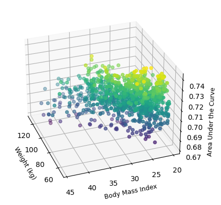
(a) All participants

(b) Male participants

Figure 3: Three-Dimensional scatter plot illustrating the area under the curve for weight and body mass index in the NHANES Dataset.

A.2 Fasting plasma glucose prediction in India

The Annual Health Survey (AHS) by the Government of India, conducted from July 2010 to May 2013, focused on nine states with high fertility and mortality rates. These states account for about 48% of India’s population, significantly contributing to global neonatal mortality.

Data and Variables

The analysis focuses on predicting the mean and variance of fasting glucose values (FPG) using a subset of 620,012 patients and $p=9$ predictors, highlighting the importance of FPG in diagnosing and monitoring diabetes progression in low-economy settings and disparaties and inequiality to the acess of healthy system.

Public Health Relevance

The AHS offers vital data for addressing health challenges in India. With the rising prevalence of diabetes, a predictive model for fasting glucose values is crucial for diabetes screening. This is particularly pertinent in India, which has one of the highest diabetes populations globally.

Results

Variable name			Men		Women
	$\overline{x}$	$\hat{v}$	$\overline{x}$	$\hat{v}$	$\overline{x}$	$\hat{v}$
Age	✓		✓		✓	✓
Weight	✓	✓		✓
Height		✓		✓		✓
haemoglobin_level	✓	✓		✓		✓
bp_systolic		✓				✓
bp_diastolic		✓				✓
pulse_rate	✓	✓		✓		✓
bmi		✓

Table 12: Feature selection in CAB dataset in the tested configurations, where weight is in kilograms, height in centimeters, the haemoglobin level is in grams per deciliter (g/dL), blood pressure systolic and the blood pressure diastolic are expressed in millimeters of mercury (mmHg), and the pulse rate refers to the number of heartbeats per minute.

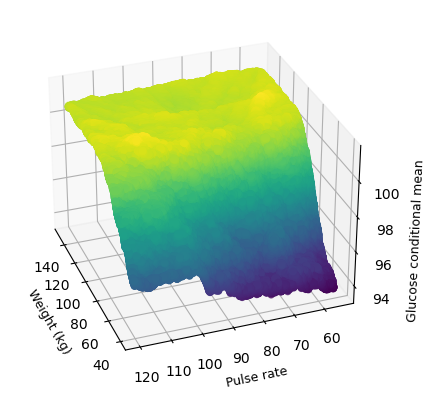
(a) Conditional mean among all participants.

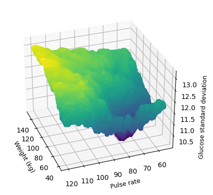
(b) Conditional standard deviation among all participants.

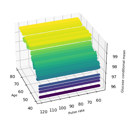
(c) Conditional mean among male participants.

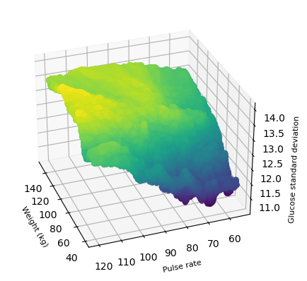
(d) Conditional standard deviation among male participants.

Figure 4: Three-Dimensional scatter plot illustrating the predicted glucose for weight and pulse rate among all participants in the CAD Dataset.

A.3 NHANES physical activity

We used data from the NHANES waves 2011–2014. The NHANES aims at providing a broad range of descriptive health and nutrition statistics of the U.S population. Data collection consists of an interview and an examination. Additionally, in NHANES 2011-2014 participants were asked to wear a physical activity monitor at maximun of ten days.

Data and Variables

We used a subset of $n=5011$ individuals, and $p=3$ variables, sex, age and body mass index to predict the variable Total activity count (TAC) derived from the acceleromter monitor that measure the average physical activity levels in a given time. We focus on estimate conditional and variance for such variable.

Public Health Relevance

Physical inactivity is one of the main public health concerns worldwide, having a significant impact on chronic diseases such as diabetes. Designing new personalized methods to identify abnormal behaviors in patients regarding physical activity plays a crucial role in monitoring and implementing new precision public health policies

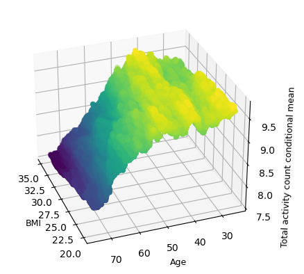
(a) Conditional mean among male participants.

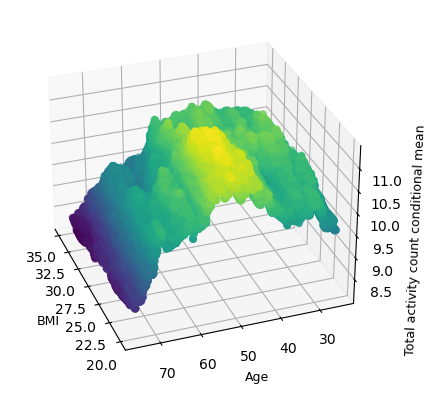
(b) Conditional mean among female participants.

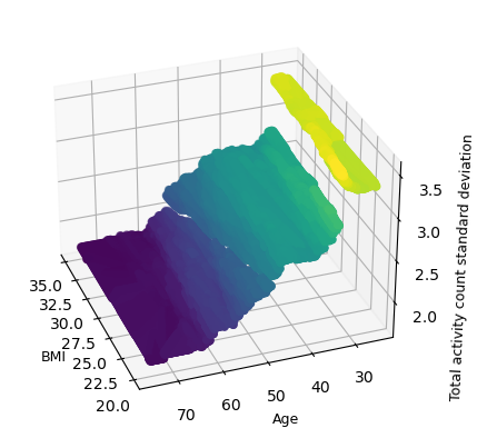
(c) Conditional standard deviation among female participants.

Figure 5: Three-Dimensional scatter plot illustrating the predicted total activity count conditional mean and standard deviation for age and body mass index in the NHANES PA Dataset.

Appendix B Details of kNN

B.1 Guarantees in Selection of Smoothing Parameters

Following [Azadkia, 2019], we distinguish between $k^{*}$ and data-computed $\tilde{k}$ in $k$-NN regression. The method for selecting $k$, namely leave-one-out cross-validation (LOOCV), is pivotal. The main result, encapsulated in the following theorem, asserts a close proximity between the mean squared errors (MSE) of $k^{*}$ and $\tilde{k}$:

$$\left|\operatorname{MSE}\left(k^{*}\right)-\operatorname{MSE}(\tilde{k})\right|=O\left(\sqrt{\frac{\log n}{n}}\right),$$

valid for fixed $K$ and $d$, without requiring additional conditions.

Theorem 2.1. Given $K$, $k^{*}$, $\tilde{k}$, and $\boldsymbol{\mu}=\left(\mu_{1},\ldots,\mu_{n}\right)$ with $\mu_{i}=m\left(\mathbf{x}_{i}\right)$, there exist positive constants $A,B,C$ (dependent on $d$ and $K$), ensuring for any $t\geq 0$:

$$\mathbb{P}\left(\left|\operatorname{MSE}\left(k^{*}\right)-\operatorname{MSE}(\tilde{k})\right|\geq t\right)\leq$$

$$\quad 4n\exp\left(-n\min\left\{At^{2},Bt\right\}\right)+4n\exp\left(-Cn^{2}t^{2}/\|\boldsymbol{\mu}\|^{2}\right).$$

This theorem implies LOOCV’s adaptability to the regression function $m$’s smoothness, as the bound is independent of $m$’s smoothness. In many cases, $\operatorname{MSE}\left(k^{*}\right)$ significantly exceeds $n^{-1/2}(\log n)^{1/2}$. For instance, [Györfi et al., 2002] shows that for Lipschitz functions with bounded support, the lower minimax MSE rate of convergence is $O\left(n^{-2/(2+d)}\right)$ for $d\geq 3$, indicating $\operatorname{MSE}\left(k^{*}\right)/\operatorname{MSE}(\tilde{k})\rightarrow 1$ as $n\rightarrow\infty$.

B.2 Computational complexity

All models described in Sections 3.1 to 3.7 exhibit quasi-linear computational complexity. This encompasses mean estimations, quantile estimations, and calculations of the inverse of discrete functions. However, the most computationally challenging aspect is the use of the kNN algorithm, which involves calculating pairwise distances $d_{ij}=|X_{i}-X_{j}|$, for $i,j=1,\dots,n$.

To enhance computational scalability, we adopt the data-splitting strategy outlined in Section 3.5. Additionally, we utilize the specific kNN library Faiss-cpu 1.7.2, which enables the rapid computation of a tree kNN structure for datasets containing up to $200$ million data points in less than a minute.

B.3 Software

B.3.1 Software and Data

Software and libraries. Our KNN model was implemented in Python 3.8.13, utilizing Faiss-cpu 1.7.2 and NumPy 1.22. For hyperparameter tuning, we employed Scikit-learn 1.0.2.

Hardware specifications. Computations were primary performed on Intel Xeon Gold 6248 (20 cores).

References

- [Akritas and Van Keilegom, 2001] Akritas, M. G. and Van Keilegom, I. (2001). Non-parametric estimation of the residual distribution. Scandinavian Journal of Statistics, 28(3):549–567.
- [Andoni et al., 2019] Andoni, A., Indyk, P., and Razenshteyn, I. (2019). Approximate nearest neighbor search in high dimensions. In Proceedings of the International Congress of Mathematicians (ICM 2018), pages 3287–3318.
- [Azadkia, 2019] Azadkia, M. (2019). Optimal choice of for -nearest neighbor regression. arXiv preprint:1909.05495.
- [Barber et al., 2023] Barber, R. F., Candes, E. J., Ramdas, A., and Tibshirani, R. J. (2023). Conformal prediction beyond exchangeability. The Annals of Statistics, 51(2):816–845.
- [Barnwal et al., 2022] Barnwal, A., Cho, H., and Hocking, T. (2022). Survival regression with accelerated failure time model in xgboost. Journal of Computational and Graphical Statistics, 31(4):1292–1302.
- [Bartlett et al., 2021] Bartlett, P. L., Montanari, A., and Rakhlin, A. (2021). Deep learning: a statistical viewpoint. Acta numerica, 30:87–201.
- [Berrett et al., 2019] Berrett, T. B., Samworth, R. J., and Yuan, M. (2019). Efficient multivariate entropy estimation via -nearest neighbour distances. The Annals of Statistics, 47(1):288 – 318.
- [Bertsimas et al., 2020] Bertsimas, D., Pauphilet, J., and Van Parys, B. (2020). Sparse regression: Scalable algorithms and empirical performance. Statistical Science, 35(4).
- [Beyerlein, 2014] Beyerlein, A. (2014). Quantile Regression—Opportunities and Challenges From a User’s Perspective. American Journal of Epidemiology, 180(3):330–331.
- [Biau et al., 2010] Biau, G., Bleakley, K., Györfi, L., and Ottucsák, G. (2010). Nonparametric sequential prediction of time series. Journal of Nonparametric Statistics, 22(3):297–317.
- [Biau and Devroye, 2015] Biau, G. and Devroye, L. (2015). Lectures on the nearest neighbor method, volume 246. Springer.
- [Brzyski et al., 2017] Brzyski, D., Peterson, C. B., Sobczyk, P., Candès, E. J., Bogdan, M., and Sabatti, C. (2017). Controlling the rate of gwas false discoveries. Genetics, 205(1):61–75.
- [Cai and Pepe, 2002] Cai, T. and Pepe, M. S. (2002). Semiparametric receiver operating characteristic analysis to evaluate biomarkers for disease. Journal of the American Statistical Association, 97(460):1099–1107.
- [Chen, 2019] Chen, G. (2019). Nearest neighbor and kernel survival analysis: Nonasymptotic error bounds and strong consistency rates. In Proceedings of the 36th International Conference on Machine Learning, pages 1001–1010.
- [Chen et al., 2018] Chen, G. H., Shah, D., et al. (2018). Explaining the success of nearest neighbor methods in prediction. Foundations and Trends in Machine Learning, 10(5-6):337–588.
- [Chernozhukov et al., 2015] Chernozhukov, V., Hansen, C., and Spindler, M. (2015). Valid post-selection and post-regularization inference: An elementary, general approach. Annu. Rev. Econ., 7(1):649–688.
- [Cohen and Kontorovich, 2022] Cohen, D. T. and Kontorovich, A. (2022). Metric-valued regression. arXiv preprint:2202.03045.
- [Collomb, 1981] Collomb, G. (1981). Estimation non-paramétrique de la régression: Revue bibliographique. International Statistical Review, 49:75–93.
- [Cover and Hart, 1967] Cover, T. and Hart, P. (1967). Nearest neighbor pattern classification. IEEE transactions on information theory, 13(1):21–27.
- [Cox, 1972] Cox, D. R. (1972). Regression models and life-tables. Journal of the Royal Statistical Society: Series B (Methodological), 34(2):187–202.
- [Csorgo et al., 1986] Csorgo, M., Csorgo, S., Horváth, L., and Mason, D. M. (1986). Weighted empirical and quantile processes. The Annals of Probability, 14(1):31–85.
- [Devroye et al., 2018] Devroye, L., Györfi, L., Lugosi, G., and Walk, H. (2018). A nearest neighbor estimate of the residual variance. Electronic Journal of Statistics, 12:1752–1778.
- [Devroye, 1978] Devroye, L. P. (1978). The uniform convergence of the nadaraya-watson regression function estimate. Canadian Journal of Statistics, 6(2):179–191.
- [Dombry et al., 2023] Dombry, C., Modeste, T., and Pic, R. (2023). Stone’s theorem for distributional regression in wasserstein distance. arXiv preprint:2302.00975.
- [Fan, 2018] Fan, J. (2018). Local polynomial modelling and its applications: monographs on statistics and applied probability, volume 66. CRC Press.
- [Fix and Hodges, 1989] Fix, E. and Hodges, J. L. (1989). Discriminatory analysis. nonparametric discrimination: Consistency properties. International Statistical Review, 57(3):238–247.
- [Goldfeld and Quandt, 1965] Goldfeld, S. M. and Quandt, R. E. (1965). Some tests for homoscedasticity. Journal of the American Statistical Association, 60(310):539–547.
- [Grams and Serfling, 1973] Grams, W. F. and Serfling, R. (1973). Convergence rates for u-statistics and related statistics. The Annals of Statistics, 1(1):153–160.
- [Guyon and Elisseeff, 2003] Guyon, I. and Elisseeff, A. (2003). An introduction to variable and feature selection. Journal of Machine Learning Research, 3:1157–1182.
- [Györfi et al., 2002] Györfi, L., Kohler, M., Krzyzak, A., Walk, H., et al. (2002). A distribution-free theory of nonparametric regression, volume 1. Springer.
- [Györfi et al., 2023] Györfi, L., Linder, T., and Walk, H. (2023). Distribution-free tests for lossless feature selection in classification and regression. arXiv preprint:2311.05033.
- [Gyôrfi and Walk, 2019] Gyôrfi, L. and Walk, H. (2019). Nearest neighbor based conformal prediction. Mathematik, 63(2):173–190.
- [Györfi and Weiss, 2021] Györfi, L. and Weiss, R. (2021). Universal consistency and rates of convergence of multiclass prototype algorithms in metric spaces. Journal of Machine Learning Research, 22:6702–6726.
- [Hall et al., 1999] Hall, P., Wolff, R. C., and Yao, Q. (1999). Methods for estimating a conditional distribution function. Journal of the American Statistical Association, 94(445):154–163.
- [Härdle and Bowman, 1988] Härdle, W. and Bowman, A. W. (1988). Bootstrapping in nonparametric regression: local adaptive smoothing and confidence bands. Journal of the American Statistical Association, 83(401):102–110.
- [Janssen, 2000] Janssen, A. (2000). Global power functions of goodness of fit tests. The Annals of Statistics, 28(1):239–253.
- [Jenkins et al., 2024] Jenkins, D. J. A. et al. (2024). Association of glycaemic index and glycaemic load with type 2 diabetes, cardiovascular disease, cancer, and all-cause mortality: a meta-analysis of mega cohorts of more than 100,000 participants. The Lancet Diabetes & Endocrinology, 12(2):107–118.
- [Jiang, 2019] Jiang, H. (2019). Non-asymptotic uniform rates of consistency for k-nn regression. In Proceedings of the AAAI Conference on Artificial Intelligence, volume 33, pages 3999–4006.
- [Joel, 2021] Joel, D. (2021). Beyond the binary: Rethinking sex and the brain. Neuroscience & Biobehavioral Reviews, 122:165–175.
- [Ju et al., 2015] Ju, C., Duan, Y., and You, X. (2015). Retesting the greater male variability hypothesis in mainland china: A cross-regional study. Personality and Individual Differences, 72:85–89.
- [Kara et al., 2017] Kara, L.-Z., Laksaci, A., Rachdi, M., and Vieu, P. (2017). Data-driven knn estimation in nonparametric functional data analysis. Journal of Multivariate Analysis, 153:176–188.
- [Klein, 2024] Klein, N. (2024). Distributional regression for data analysis. Annual Review of Statistics and Its Application, 11.
- [Kneib et al., 2023] Kneib, T., Silbersdorff, A., and Säfken, B. (2023). Rage against the mean–a review of distributional regression approaches. Econometrics and Statistics, 26:99–123.
- [Koenker, 2005] Koenker, R. (2005). Quantile regression [m]. Econometric Society Monographs, Cambridge University Press, Cambridge.
- [Kosorok, 2008] Kosorok, M. R. (2008). Introduction to empirical processes and semiparametric inference, volume 61. Springer.
- [Kozachenko and Leonenko, 1987] Kozachenko, L. F. and Leonenko, N. N. (1987). Sample estimate of the entropy of a random vector. Problemy Peredachi Informatsii, 23(2):9–16.
- [Kpotufe, 2011] Kpotufe, S. (2011). k-NN regression adapts to local intrinsic dimension. Advances in Neural Information Processing Systems, 24.
- [Kulasingam and Diamandis, 2008] Kulasingam, V. and Diamandis, E. P. (2008). Strategies for discovering novel cancer biomarkers through utilization of emerging technologies. Nature Clinical Practice Oncology, 5(10):588–599.
- [Lei et al., 2018] Lei, J., G’Sell, M., Rinaldo, A., Tibshirani, R. J., and Wasserman, L. (2018). Distribution-free predictive inference for regression. Journal of the American Statistical Association, 113(523):1094–1111.
- [Li et al., 2021] Li, W., Zhang, C., Tsung, F., and Mei, Y. (2021). Nonparametric monitoring of multivariate data via knn learning. International Journal of Production Research, 59(20):6311–6326.
- [Meixide et al., 2022] Meixide, C. G., Matabuena, M., and Kosorok, M. R. (2022). Neural interval-censored cox regression with feature selection. arXiv preprint:2206.06885.
- [Mu and He, 2007] Mu, Y. and He, X. (2007). Power transformation toward a linear regression quantile. Journal of the American Statistical Association, 102(477):269–279.
- [Müller and Stadtmüller, 1993] Müller, H.-G. and Stadtmüller, U. (1993). On variance function estimation with quadratic forms. Journal of Statistical Planning and Inference, 35(2):213–231.
- [Nakas et al., 2023] Nakas, C. T., Bantis, L. E., and Gatsonis, C. A. (2023). ROC Analysis for Classification and Prediction in Practice. CRC Press.
- [Padilla, 2022] Padilla, O. H. M. (2022). Variance estimation in graphs with the fused lasso. arXiv preprint:2207.12638.
- [Pepe et al., 2008] Pepe, M. S., Feng, Z., Huang, Y., Longton, G., Prentice, R., Thompson, I. M., and Zheng, Y. (2008). Integrating the predictiveness of a marker with its performance as a classifier. American Journal of Epidemiology, 167(3):362–368.
- [Portier, 2021] Portier, F. (2021). Nearest neighbor process: weak convergence and non-asymptotic bound. arXiv preprint:2110.15083.
- [Ramdas et al., 2015] Ramdas, A., Reddi, S. J., Póczos, B., Singh, A., and Wasserman, L. (2015). On the decreasing power of kernel and distance based nonparametric hypothesis tests in high dimensions. In Proceedings of the AAAI Conference on Artificial Intelligence, volume 29.
- [Rigby and Stasinopoulos, 2005] Rigby, R. A. and Stasinopoulos, D. M. (2005). Generalized Additive Models for Location, Scale and Shape. Journal of the Royal Statistical Society Series C: Applied Statistics, 54(3):507–554.
- [Rindt et al., 2022] Rindt, D., Hu, R., Steinsaltz, D., and Sejdinovic, D. (2022). Survival regression with proper scoring rules and monotonic neural networks. In Proceedings of the 25th International Conference on Artificial Intelligence and Statistics, volume 151, pages 1190–1205.
- [Rossell et al., 2023] Rossell, D., Kseung, A. K., Saez, I., and Guindani, M. (2023). Semi-parametric local variable selection under misspecification. arXiv preprint:2401.10235.
- [Rudi et al., 2017] Rudi, A., Carratino, L., and Rosasco, L. (2017). Falkon: An optimal large scale kernel method. Advances in Neural Information Processing Systems, 30.
- [Saaristo et al., 2005] Saaristo, T. et al. (2005). Cross-sectional evaluation of the finnish diabetes risk score: a tool to identify undetected type 2 diabetes, abnormal glucose tolerance and metabolic syndrome. Diabetes and Vascular Disease Research, 2(2):67–72.
- [Serfling, 2009] Serfling, R. J. (2009). Approximation theorems of mathematical statistics. John Wiley & Sons.
- [Shafer and Vovk, 2008] Shafer, G. and Vovk, V. (2008). A tutorial on conformal prediction. Journal of Machine Learning Research, 9(3).
- [Shi et al., 2018] Shi, B., Han, L., and Yan, H. (2018). Adaptive clustering algorithm based on knn and density. Pattern Recognition Letters, 104:37–44.
- [Stone, 1977] Stone, C. J. (1977). Consistent nonparametric regression. The Annals of Statistics, 5(4):595–620.
- [Stute, 1991] Stute, W. (1991). Conditional u-statistics. The Annals of Probability, 19(2):812–825.
- [Su et al., 2018] Su, T.-L., Jaki, T., Hickey, G. L., Buchan, I., and Sperrin, M. (2018). A review of statistical updating methods for clinical prediction models. Statistical Methods in Medical Research, 27(1):185–197.
- [Verdinelli and Wasserman, 2021] Verdinelli, I. and Wasserman, L. (2021). Decorrelated variable importance. arXiv preprint:2111.10853.
- [Vural and Guillemot, 2018] Vural, E. and Guillemot, C. (2018). A study of the classification of low-dimensional data with supervised manifold learning. Journal of Machine Learning Research, 18(157):1–55.
- [Yong et al., 2009] Yong, Z., Youwen, L., and Shixiong, X. (2009). An improved knn text classification algorithm based on clustering. Journal of Computers, 4(3):230–237.
- [Zhang et al., 2017] Zhang, S., Li, X., Zong, M., Zhu, X., and Wang, R. (2017). Efficient knn classification with different numbers of nearest neighbors. IEEE Transactions on Neural Networks and Learning Systems, 29(5):1774–1785.
- [Zhang and Politis, 2023] Zhang, Y. and Politis, D. N. (2023). Bootstrap prediction intervals with asymptotic conditional validity and unconditional guarantees. Information and Inference: A Journal of the IMA, 12(1):157–209.
- [Zhao and Yang, 2023] Zhao, B. and Yang, Y. (2023). Minimax rates of convergence for nonparametric location-scale models. arXiv preprint:2307.01399.
- [Zhao and Lai, 2021] Zhao, P. and Lai, L. (2021). Minimax rate optimal adaptive nearest neighbor classification and regression. IEEE Transactions on Information Theory, 67(5):3155–3182.
- [Zhou and Kosorok, 2017] Zhou, X. and Kosorok, M. R. (2017). Causal nearest neighbor rules for optimal treatment regimes. arXiv preprint:1711.08451.