Beyond Lengthscales: No-regret Bayesian Optimisation With Unknown Hyperparameters Of Any Type

Abstract

Bayesian optimisation requires fitting a Gaussian process model, which in turn requires specifying hyperparameters—most of the theoretical literature assumes those hyperparameters are known. The commonly used maximum likelihood estimator for hyperparameters of the Gaussian process is consistent only if the data fills the space uniformly, which does not have to be the case in Bayesian optimisation. Since no guarantees exist regarding the correctness of hyperparameter estimation, and those hyperparameters can significantly affect the Gaussian process fit, theoretical analysis of Bayesian optimisation with unknown hyperparameters is very challenging. Previously proposed algorithms with the no-regret property were only able to handle the special case of unknown lengthscales, reproducing kernel Hilbert space norm and applied only to the frequentist case. We propose a novel algorithm, HE-GP-UCB, which is the first algorithm enjoying the no-regret property in the case of unknown hyperparameters of arbitrary form, and which supports both Bayesian and frequentist settings. Our proof idea is novel and can easily be extended to other variants of Bayesian optimisation. We show this by extending our algorithm to the adversarially robust optimisation setting under unknown hyperparameters. Finally, we empirically evaluate our algorithm on a set of toy problems and show that it can outperform the maximum likelihood estimator.

1 Introduction

Bayesian Optimisation (BO) (Garnett, 2023) emerged as a successful paradigm for solving black-box optimisation problems in a sample-efficient manner. It found applications in numerous fields such as drug discovery (Khan et al., 2023), logic circuit design (Grosnit et al., 2022), and tuning hyperparameters of machine learning algorithms (Cowen-Rivers et al., 2022). BO algorithms construct a surrogate model of the unknown black-box function based on the observed values for the points queried so far. The model used in most cases is the Gaussian Process (GP), which requires a specification of a prior and its hyperparameters.

These hyperparameters could, for example, be lengthscales $\theta$, which scale the input before applying the kernel, i.e. $k_{\theta}(\bm{x},\bm{x}^{\prime})=k(\frac{\bm{x}}{\theta},\frac{\bm{x}^{\prime}}{\theta})$. However, hyperparameters can come in many shapes and forms beyond just lengthscales. In high-dimensional BO, it is common to use additive kernel decompositions (Kandasamy et al., 2015; Rolland et al., 2018) of the form $k(\bm{x},\bm{x}^{\prime})=\sum_{c\in g}k_{c}(\bm{x}_{[c]},\bm{x}^{\prime}_{[c]})$, where $\bm{x}_{[c]}$ selects only the dimensions in set $c$ and $g$ is a collection of sets. This collection of sets essentially becomes a hyperparameter of the kernel. When dealing with periodic functions, the period of the function becomes a new parameter that needs to be estimated. Finally, the prior mean function can also include unknown hyperparameters, for example, we might have two candidate mean functions $\mu^{A}_{0}(\bm{x})$ and $\mu^{B}_{0}(\bm{x})$ given to us by domain experts, and use a prior mean of $\mu_{0}(\bm{x})=Z\mu_{0}^{A}(\bm{x})+(1-Z)\mu_{0}^{B}(\bm{x})$, where $Z\in\{0,1\}$ is the unknown hyperparameter.

When analysing the performance of a BO algorithm, we are usually interested in proving a bound on its regret, which is the sum of differences between the optimal function value and the one at the queried point. To show our algorithm provably converges, we want to prove that its regret bound is sublinear in $T$, also referred to as no-regret property. GP-UCB algorithm has been proven (Srinivas et al., 2010) to enjoy a no-regret guarantee, but only if the kernel and its hyperparameter values are known.

In practice, the parameters of the kernel function are selected by the maximum likelihood estimation (MLE). Statistical literature (Bachoc, 2013) provides asymptotic consistency guarantees for MLE of kernel hyperparameters, but only in the case, where the points at which we know the function values fill the space uniformly. This does not hold for BO, which selects the points in a non-uniform manner. As such, studying the behaviour of BO with unknown kernel hyperparameters is challenging and no guarantees exist regarding the correctness of hyperparameter estimation. The no-regret proof of GP-UCB (Srinivas et al., 2010) requires that the GP model provides us with valid confidence bounds for the function values. As different hyperparameter values may produce different confidence bounds and we are unable to reliably recover the true hyperparameter value, deriving a no-regret guarantee in such a setting is very challenging.

The only two previous works (Wang & de Freitas, 2014; Berkenkamp et al., 2019) that proposed no-regret BO algorithms with unknown hyperparameters both considered the special case of unknown lengthscales (the latter also considered a special case of unknown reproducing kernel Hilbert space (RKHS) norm) and studied only the frequentist case that is when the black-box function is a member of a RKHS of some kernel $k(\cdot,\cdot)$, i.e. $f\in\mathcal{H}(k)$. In their algorithms, the lengthscale hyperparameter is progressively shrunk. This shrinking is done regardless of the observed data. The algorithms enjoy the no-regret property, as for two lengthscales $\theta_{1}\leq\theta_{2}$, in the case that $f\in\mathcal{H}(k_{\theta_{2}})\implies f\in\mathcal{H}(k_{\theta_{1}})$, where $\mathcal{H}(k_{\theta})$ is the RKHS defined by kernel $k_{\theta}$ with lengthscale $\theta$. As a result, if the lengthscale is small enough, the true function has to lie in the RKHS of the used kernel and the confidence bounds of the resulting models are valid. In the case of arbitrary hyperparameters, such a strategy will not work, as it is possible that RKHS of two hyperparameter values do not encapsulate one another. This means that there exists a function such that $f\in\mathcal{H}(k_{u})$ but $f\notin\mathcal{H}(k_{v})$ and vice versa for two hyperparameter values $u$ and $v$. Moreover, this strategy will also not work in the Bayesian case that is when the black-box function is a sample from a GP prior. This is because if the black-box function is a sample from prior with lengthscale $\theta_{2}$, i.e. $f\sim\mathcal{GP}_{\theta_{2}}$, then that exact prior needs to be used to produce a valid posterior. It cannot be replaced by $\mathcal{GP}_{\theta_{1}}$ for some shorter lengthscale $\theta_{1}<\theta_{2}$.

In this work, we propose the first BO algorithm which enjoys the no-regret property in both Bayesian and frequentist settings with unknown hyperparameters of arbitrary form, as long as there is a finite set of candidate hyperparameter values. Our algorithm effectively eliminates hyperparameter values that are highly implausible given the data observed so far, making it also the first no-regret algorithm with data-driven hyperparameter updates. When selecting the next point to query, our algorithm is optimistic with respect to the hyperparameter values that have not yet been eliminated. Our proof technique is novel and relies on the idea that if all hyperparameter values produce models explaining the observations well enough then it does not matter which is used. On the other hand, if this is not the case then we can easily eliminate wrong models. Importantly, our proof technique is very universal and we believe it can be easily extended to different variants of standard BO. We show one concrete example, by extending our method to deal with adversarially robust optimisation.

Contributions

• We propose the HE-GP-UCB, the first no-regret algorithm which:

  • can handle arbitrary hyperparameters of any form

  • works also in the Bayesian setting

  • employs data-driven hyperparameter updates.

• Our proof idea is novel and easily extendable to other variants of BO. We show this by developing HE-StableOpt, which is a version of HE-GP-UCB capable of performing adversarially robust optimisation under unknown hyperparameters.

• We empirically compare the performance of our algorithm to other algorithms on a set of toy problems and show that it can outperform MLE.

Related work on Bayesian Optimisation As mentioned before, the seminal no-regret proofs of GP-UCB (Srinivas et al., 2010) and IGP-UCB(Chowdhury & Gopalan, 2017) assumed the true hyperparameter value is known. Bull (2011) derived a bound on simple regret of BO with unknown lengthscales and output scales on noiseless functions, but without cumulative regret bound. Hoffman et al. (2011) proposed an adversarial bandit-style algorithm GP-HEDGE for problems, where the parameters of the acquisition function are unknown. Although they provide a cumulative regret bound, they also admit that it is not sublinear. In the case of unknown lengthscales, the aforementioned works of Wang & de Freitas (2014); Berkenkamp et al. (2019) proposed algorithms with sublinear regret. However, as explained before, these algorithms cannot be extended to deal with unknown hyperparameters of arbitrary form and do not work in the Bayesian case. More recently, Ha et al. (2023) proposed the UHE-BO algorithm for unknown hyperparameter BO and provided simple regret guarantees, but without guarantees on cumulative regret. As UHE-BO relies on sampling random points, it is unlikely for it to have the no-regret property. Hvarfner et al. (2023) proposed ScoreBO algorithm, which combines BO with an active learning strategy to learn the hyperparameter values. However, they provide no theoretical analysis of the proposed algorithm.

Related work on Master Algorithms in Bandits Within the multi-armed bandits community, it is common to study a problem, in which we are supposed to design a master algorithm to coordinate a number of base algorithms (Agarwal et al., 2017; Abbasi-Yadkori et al., 2020; Pacchiano et al., 2020; Moradipari et al., 2022). A natural question that arises is whether we could extend those algorithms to BO settings and run such a master algorithm with one base algorithm for each possible value of the hyperparameter. However, as explained in Appendix A, such constructed algorithms either do not achieve no-regret property or apply only to very special cases. On the other hand, the algorithm we propose later achieves no-regret property under the general case of unknown hyperparameters of any form.

Table 1: Comparison of different BO algorithms and their abilities to deal with unknown hyperparameters. The notation $\tilde{\mathcal{O}}(\cdot)$ hides logarithmic factors for brevity. If logarithmic factors were not hidden, the frequentist bound of IGP-UCB would be better than that of GP-UCB. A-GP-UCB is the method of Berkenkamp et al. (2019) and BOHO is the method of Wang & de Freitas (2014). $A_{\theta}^{B}=\max\left\{g^{-1}(\underset{i}{\max}\frac{\theta_{0}}{\theta}),b^{-1}(\frac{B}{B_{0}})\right\}$, where $\theta_{0}$ and $B_{0}$ are upper and lower bounds on lengthscale and RKHS norm respectively and $\theta$ and $B$ are the true values of those quantities; $g(\cdot)$ and $b(\cdot)$ are some functions that increase without bound. $\theta_{T}$ is the shortest lengthscale considered by A-GP-UCB by time $T$ and $\theta_{L}$ is some known lower-bound on lengthscale hyperparameter. We define by $\hat{\gamma_{T}}=\max_{u\in U}\gamma_{T}^{u}$ and $E=\min\{d,\log|\mathcal{X}|\}$. LS stands for lengthscale.

Algorithm	Unknown	frequentist	Bayesian	Hypers.
	hypers.	$R_{T}$ bound	$R_{T}$ bound	updates
GP-UCB	✗	$\tilde{\mathcal{O}}(\sqrt{T}(B\sqrt{\gamma_{T}}+\gamma_{T}))$	$\tilde{\mathcal{O}}(\sqrt{T\gamma_{T}E})$	✗
IGP-UCB	✗	$\tilde{\mathcal{O}}(\sqrt{T}(B\sqrt{\gamma_{T}}+\gamma_{T}))$	✗	✗
BOHO	LS	$\tilde{\mathcal{O}}(\sqrt{T}(B\sqrt{\gamma_{T}^{\theta_{L}}}+\gamma_{T}^{\theta_{L}}))$	✗	pre-defined
A-GP-UCB	LS/ RKHS norm	$\tilde{\mathcal{O}}\left(A_{\theta}^{B}B+\sqrt{T}(B\sqrt{\gamma_{T}^{\theta_{T}}}+\gamma_{T}^{\theta_{T}})\right)$	✗	pre-defined
HE-GP-UCB (ours)	Any	$\tilde{\mathcal{O}}\left(|U|B+\sqrt{T}(B\sqrt{\hat{\gamma_{T}}}+\hat{\gamma}_{T})\right)$	$\tilde{\mathcal{O}}(|U|B+\sqrt{T\hat{\gamma}_{T}E})$	data-driven

2 Problem Statement

We consider a standard problem setting where we wish to maximise an unknown, black-box function $f:\mathcal{X}\to\mathbb{R}$ over some compact set $\mathcal{X}\subset\mathbb{R}^{d}$, i.e. $\max_{\bm{x}\in\mathcal{X}}f(\bm{x})$. We assume we are allowed to query a single point $\bm{x}_{t}$ at each timestep $t$ and obtain its function value corrupted by some i.i.d. noise $\epsilon_{t}$, i.e. $y_{t}=f(\bm{x}_{t})+\epsilon_{t}$. The exact distribution of that noise will depend on whether we are in Bayesian or frequentist settings, as defined later. As we want to maximise the function, the instantaneous regret is defined as $r_{t}=f(\bm{x}^{*})-f(\bm{x}_{t})$, where $\bm{x}^{*}=\arg\max_{\bm{x}\in\mathcal{X}}f(\bm{x})$. Similarly, we define cumulative regret as $R_{T}=\sum_{t=1}^{T}r_{t}$. We also assume there is some ”true” hyperparameter value $u^{*}\in U$ associated with the function $f$, formally defined later. Typically in literature, it was assumed (Srinivas et al., 2010; Chowdhury & Gopalan, 2017) that the true hyperparameter value is known, but in this work, we lift this assumption. We assume we have access to $U$ and $|U|<\infty$, but we do not know which element of $U$ is the true hyperparameter value.

Why do we need to assume $|U|<\infty$? Consider the case when $|U|=\infty$. There is always an infinite number of functions going through any finite number of points. At each timestep, we could thus have an infinite number of hyperparameter values producing models explaining our observations equally well, but differing significantly when it comes to unexplored regions. Without any strong assumptions about the smoothness of the mapping from hyperparameter values to mean and variance functions of the fitted GP, obtaining the no-regret property would be impossible. Notice that there are some settings, where the hyperparameter is naturally discrete, for example in the aforementioned high-dimensional BO when we want to choose one of the possible additive decompositions of the kernel function. We now distinguish between two problem settings.

Bayesian Setting In Bayesian setting, we assume our black-box function $f$ was sampled from a GP prior, i.e. $f\sim\mathcal{GP}(\mu_{0}^{u^{*}}(\cdot),k^{u^{*}}(\cdot,\cdot))$ for some mean function $\mu_{0}^{u^{*}}(\cdot)$ and kernel function $k_{0}^{u^{*}}(\cdot)$ parametrised by some $u^{*}\in U$, which we call true hyperparameter value. We require $\sup_{\bm{x}\in\mathcal{X}}\mu^{u}_{t-1}(\bm{x})<\infty$ for each $u\in U$. We further assume the distribution of noise is $\epsilon_{t}\sim\mathcal{N}(0,R^{2})$.

Frequentist Setting In frequentist setting, we assume that the true black-box function $f\in\mathcal{H}(k^{u^{*}})$, where $\mathcal{H}(k^{u^{*}})$ is the RKHS of kernel $k^{u^{*}}(\cdot,\cdot)$ for some $u^{*}\in U$, which we call true hyperparameter value. We assume the noise $\epsilon_{t}$ has some $R$-subgaussian distribution.

In both cases, without the loss of generality, we assume that $k^{u}(\cdot,\cdot)\leq 1$ for all $u\in U$. As the regret depends on the kernel $k^{u^{*}}(\cdot,\cdot)$, typically in BO literature, the regret bound is expressed in terms of maximum information gain (MIG) (Srinivas et al., 2010) of kernel $k^{u^{*}}$, defined as $\gamma_{T}^{u^{*}}:=\max_{A\subseteq\mathcal{X}:|A|=T}\frac{1}{2}\log\lvert I+R^{-2}\bm{K}^{u^{*}}_{A}\rvert$, where $\bm{K}^{u^{*}}_{A}=[k^{u^{*}}(\bm{x},\bm{x}^{\prime})]_{\bm{x},\bm{x}^{\prime}\in A}$. Fortunately, $\gamma_{T}^{u^{*}}$ is sublinear in $T$ for commonly used kernels.

Gaussian Process Model In BO, at each timestep $t$, we contruct a surrogate model of the black-box function, based on the queries so far. Let $\mathcal{D}_{t-1}=\{(\bm{x}_{i},y_{i})\}_{i=1}^{t-1}$ be the collection of all queried points and their corresponding noisy values up to timestep $t-1$. If we use a GP model with a kernel $k^{u}(\bm{x},\bm{x}^{\prime})$, where $u$ is the kernel hyperparameter, then given the data so far $\mathcal{D}_{t-1}$, the model returns us the following mean $\mu^{u}_{t-1}(\bm{x})$ and variance $(\sigma^{u}_{t-1})^{2}(\bm{x})$ functions:

$$\mu^{u}_{t-1}(\bm{x})=\bm{k}^{u}_{t-1}(\bm{x})^{T}(\mathbf{K}^{u}_{t-1}+R^{2}\mathbf{I})^{-1}\bm{y}_{t-1}$$

$$(\sigma^{u}_{t-1})^{2}(\bm{x})=k(\bm{x},\bm{x})^{u}-\bm{k}^{u}_{t-1}(\bm{x})^{T}(\mathbf{K}^{u}_{t-1}+R^{2}\mathbf{I})^{-1}\bm{k}^{u}_{t-1}(\bm{x}),$$

where $\bm{y}_{t-1}\in\mathbb{R}^{t-1}$ with elements $(\bm{y})_{i}=y_{i}$, $\bm{k}^{u}(\bm{x})\in\mathbb{R}^{t-1}$ with elements $\bm{k}^{u}(\bm{x})_{i}=k^{u}(\bm{x},\bm{x}_{i})$ and similarily $\mathbf{K}^{u}_{t-1}\in\mathbb{R}^{t-1\times t-1}$ with entries $\mathbf{K}^{u}_{i,j}=k^{u}(\bm{x}_{i},\bm{x}_{j})$. While using mean and variance functions provided by the GP, we get the guarantee on predictive performance in Bayesian and frequentist settings, as stated in the next Section.

3 Preliminaries

We now recall well-known results from the literature. Those results would be later needed to prove the no-regret property of our proposed algorithm.

Theorem 3.1.

Let either of the following two be the case:

• Assume the Bayesian setting and let $f\sim\mathcal{GP}\left(\mu_{0}^{u^{*}}(\cdot),k^{u^{*}}(\cdot,\cdot)\right)$, and set $\beta^{u^{*}}_{t}=\sqrt{2\log\left(\frac{|\mathcal{X}|\pi^{2}t^{2}}{6\delta_{A}}\right)}$

• Assume the frequentist setting and let $f\in\mathcal{H}\left(k^{u^{*}}\right)$, such that $\lVert f\rVert_{k^{u^{*}}}\leq B$ and set $\beta^{u^{*}}_{t}=B+R\sqrt{2(\gamma^{u^{*}}_{t-1}+1+\ln(1/\delta_{A}))}$

Then, with probability at least $1-\delta_{A}$, for all $\bm{x}\in\mathcal{X}$ and $t=1,\dots,T$:

$$\left|f(\bm{x})-\mu_{t-1}^{u^{*}}(\bm{x})\right|\leq\beta^{u^{*}}_{t}\sigma_{t-1}^{u^{*}}(\bm{x}).$$

Proof.

Bayesian case follows from Lemma 5.1 of Srinivas et al. (2010) and frequentist case from Theorem 2 of Chowdhury & Gopalan (2017). ∎

Note that the confidence parameter $\beta_{t}$ in Theorem 3.1, depends on $|\mathcal{X}|$ in the Bayesian setting and only makes sense if $|\mathcal{X}|<\infty$. If this is not the case, we need to adopt a standard assumption (Srinivas et al., 2010), stated in Appendix B. Under that assumption, we can derive high-probability confidence intervals in the Bayesian case even if $|\mathcal{X}|=\infty$. Following Srinivas et al. (2010), purely for the sake of analysis, let us define a discretization $D_{t}$ of size $(\tau_{t})^{d}$ so that for all $x\in D_{t}$, $\lVert x-[x]_{t}\rVert_{1}\leq\frac{r}{d\tau_{t}}$, where $[x]_{t}$ denotes the closest point in $D_{t}$ to $x$. We now get the following Theorem.

Theorem 3.2.

Let Assumption B.1 hold, set $\beta_{t}^{u^{*}}=\sqrt{2\log\left(\frac{\pi^{2}t^{2}}{3\delta_{A}}\right)+2d\log\left(dt^{2}br\sqrt{\log\left(\frac{2da}{\delta_{A}}\right)}\right)}$ and set the size of discretisation to $\tau_{t}=dt^{2}br\sqrt{\log\left(\frac{2da}{\delta_{A}}\right)}$. Then with probability at least $1-\delta_{A}$ we have for all $\bm{x}\in\mathcal{X}$:

$$|f(\bm{x})-\mu_{t-1}^{u^{*}}([\bm{x}]_{t})|\leq\beta_{t}^{u^{*}}\sigma^{u^{*}}_{t-1}([\bm{x}]_{t})+\frac{1}{t^{2}}$$

And for any $\bm{x}_{t}$ deterministic conditioned on $(y_{i},\bm{x}_{i})_{i=1}^{t-1}$ :

$$|f(\bm{x}_{t})-\mu_{t-1}^{u^{*}}(\bm{x}_{t})|\leq\beta_{t}^{u^{*}}\sigma^{u^{*}}_{t-1}(\bm{x}_{t}).$$

Proof.

Lemma 5.5 and 5.7 of Srinivas et al. (2010). ∎

4 GP-UCB with Hyperparameter Elimination

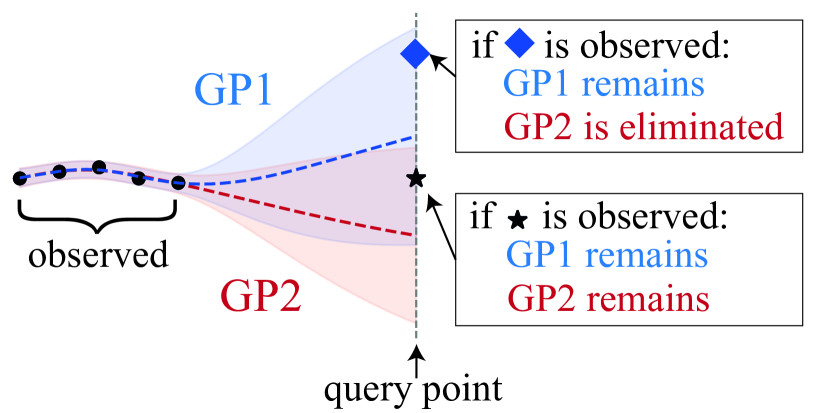
Figure 1: Intuition behind the hyperparameter elimination. Solid lines represent the mean functions of two models - GP1 and GP2, produced by fitting the observed points with different hyperparameter values, and shaded regions are confidence intervals. The point marked by the star lies in the confidence intervals of both models, whereas the point marked by the diamond lies in the one of GP1.

We now state our proposed algorithm in Algorithm 1. Algorithm 1 solves both Bayesian and frequentist settings with unknown hyperparameters, making it the first algorithm to achieve sublinear regret under such conditions, to the best of our knowledge. When selecting the next point to query (line 7), our algorithm is doubly optimistic, with respect to both the function value and the model. In other words, for each point, we use the best possible upper confidence bound among the ones suggested by models defined by hyperparameter values in $U_{t-1}$. We denote the selected point by $\bm{x}_{t}$ and the hyperparameter value under which it achieved the highest UCB value is denoted by $u_{t}$. The set $S^{u}_{t}$ stores all iterations $i$ up to the current one $t$, during which $u_{i}=u$, for each $u\in U$ (line 8). After observing the function value, we calculate the error $\eta_{t}$ between the observed value and the mean at point $\bm{x}_{t}$, according to the model defined by $u_{t}$ (line 11). Then, each model for which the sum of errors is too big is removed from the set of candidates (lines 12-14) and we continue with the loop.

The intuition behind this mechanism is depicted in Figure 1. Let us assume we have two models GP1 and GP2, represented by red and blue solid lines, together with their corresponding confidence intervals in dashed lines. After we query a new point, it can either lie within the confidence intervals of both models (like the star) or only one model (like the diamond). If we were to obtain a point like the diamond, we clearly see that the red model’s prediction was very inaccurate and we lean towards rejecting the hyperparameter value that produced it. On the other hand, if we observe a point like the star when querying the function then it does not matter, which model is the ”true” one, as such an observation is probable under both models and the errors for either of the models would be small. Thanks to this mechanism, we can conduct BO, whilst simultaneously estimating the hyperparameter values. Such a strategy achieves the no-regret property in both Bayesian and frequentist settings. We first state the frequentist result.

Algorithm 1 Hyperparameter Elimination GP-UCB
(HE-GP-UCB)

0:  a set of possible hyperparameter values $U$; confidence parameters $\{\xi_{t}\}_{t=1}^{T}$ and $\{\{\beta^{u}_{t}\}_{t=1}^{T}\}_{u\in U}$

1:  Set $\mathcal{D}_{0}=\emptyset$, $U_{0}=U$, $S^{u}=\emptyset$ for each $u\in U$

2:  for $t=1,\dots,T$ do

3:     for $u\in U_{t-1}$ do

4:        Fit a GP $(\mu^{u}_{t-1}(\bm{x}),\sigma^{u}_{t-1}(\bm{x}))$ to $\mathcal{D}_{t-1}$

5:        Set $\textrm{UCB}_{t-1}^{u}(\bm{x})=\mu^{u}_{t-1}(\bm{x})+\beta_{t}^{u}\sigma^{u}_{t-1}(\bm{x})$

6:     end for

7:     Find $\bm{x}_{t},u_{t}=\underset{\bm{x},u\in\mathcal{X}\times U_{t-1}}{\arg\max}\textrm{UCB}_{t-1}^{u}(\bm{x})$

8:     $S^{u_{t}}_{t}=S^{u_{t}}_{t-1}\cup\{t\}$ and $S^{u}_{t}=S^{u}_{t-1}$ for $u\in U;u\neq u_{t}$

9:     Query the black-box $y_{t}=f(x_{t})$

10:     Set $\mathcal{D}_{t}=\mathcal{D}_{t-1}\cup(x_{t},y_{t})$

11:     Set $\eta_{t}=y_{t}-\mu^{u_{t}}_{t-1}(\bm{x}_{t})$

12:     if $\left|\sum_{i\in S^{u_{t}}_{t}}\eta_{i}\right|>\sqrt{\xi_{t}|S^{u_{t}}_{t}|}+\sum_{i\in S^{u_{t}}_{t}}\beta^{u_{t}}_{i}\sigma_{i}^{u_{t}}(\bm{x}_{i})$ then

13:        $U_{t}=U_{t-1}\setminus\{u_{t}\}$

14:     end if

15:  end for

Theorem 4.1 (Frequentist setting).

Let $f\in\mathcal{H}\left(k^{u^{*}}\right)$, s.t. $\lVert f\rVert_{k^{u^{*}}}\leq B$, $u^{*}\in U$ and denote $\gamma_{T}=\max_{u\in U}\gamma_{T}^{u}$ and $\beta_{T}=\max_{u\in U}\beta_{T}^{u}$. Set $\beta_{t}^{u}=B+R\sqrt{2(\gamma^{u}_{t-1}+1+\ln(2/\delta))}$ and $\xi_{t}=2R^{2}\log\frac{|U|\pi t^{2}}{3\delta}$. Then, Algorithm 1 with probability at least $1-\delta$ achieves the cumulative regret of at most:

$$R_{T}\leq\mathcal{O}\left(|U|B+\sqrt{|U|\xi_{T}T}+\beta_{T}\sqrt{|U|\gamma_{T}T}\right)$$

and as $\lim_{T\to 0}\frac{R_{T}}{T}\to 0$, Algorithm 1 enjoys the no-regret property.

We now turn to the Bayesian setting. We note that the exact bound depends on whether $\mathcal{X}$ is a finite set or not, but in either case, the no-regret property holds.

Theorem 4.2 (Bayesian setting).

Let $f\sim\mathcal{GP}(\mu_{0}^{u^{*}}(\cdot),k^{u^{*}}(\cdot,\cdot))$, $\epsilon_{t}\sim\mathcal{N}(0,R^{2})$ for each $t$ and $u^{*}\in U$ and denote $\gamma_{T}=\max_{u\in U}\gamma_{T}^{u}$. Set $\xi_{t}=2R^{2}\log\frac{|U|\pi^{2}t^{2}}{3\delta}$ and :

1. if $|\mathcal{X}|<\infty$, set $\beta_{t}^{u}=\sqrt{2\log\frac{|\mathcal{X}|\pi^{2}t^{2}}{3\delta}}$

2. if $|\mathcal{X}|=\infty$, let Assumption B.1 hold and set

$$\beta_{t}^{u}=\sqrt{2\log\left(\frac{2\pi^{2}t^{2}}{3\delta}\right)+4d\log\left(dtbr\sqrt{\log\left(\frac{4da}{\delta}\right)}\right)}$$

Then, Algorithm 1 with probability at least $1-\delta$ achieves the cumulative regret of at most:

$$R_{T}\leq\mathcal{O}\left(|U|B+\sqrt{|U|\xi_{T}T}+\beta_{T}\sqrt{|U|\gamma_{T}T}\right)$$

for some constant $B>0$ and as $\lim_{T\to 0}\frac{R_{T}}{T}\to 0$, Algorithm 1 enjoys the no-regret property.

5 Proof sketch of the regret bound

We provide a sketch of the proof technique in this section. For the full proof, see Appendix C and D for frequentist and Bayesian versions, respectively. We first look at the frequentist case and then comment on the differences with the Bayesian case. We first introduce the following Lemma for the concentration of noise, proved in Appendix E.

Lemma 5.1.

For each $u\in U$ and $t=1,\dots,T$ we have:

$$P\left(\underset{t=1,\dots,T}{\forall}\,\underset{u\in U}{\forall}\left|\sum_{i\in S_{t}^{u}}\epsilon_{i}\right|\leq\sqrt{\xi_{t}|S_{t}^{u}|}\right)\geq 1-\delta_{B},$$

where $\xi_{t}=2R^{2}\log\frac{|U|\pi^{2}t^{2}}{6\delta_{B}}$.

Observe that by union bound Theorem 3.1 and Lemma 5.1 hold together with probability at least $1-\delta_{A}-\delta_{B}$. We choose $\delta_{A}=\delta_{B}=\frac{\delta}{2}$. We prove the regret bound, assuming the probabilistic statements in Theorem 4.1 and Lemma 5.1 hold, and as such the resulting bound holds with probability at least $1-\delta$.

Preservation of $u^{*}$ We first show that if the statements from Theorem 3.1 and Lemma 5.1 hold, then the true hyperparameter value $u^{*}$ is never rejected. Indeed, when line 12 is executed at iteration $t$:

$$\left|\sum_{i\in S^{u^{*}}_{t}}\eta_{t}\right|=\left|\sum_{i\in S^{u^{*}}_{t}}\left(y_{t}-f(\bm{x}_{t})+f(\bm{x}_{t})-\mu^{*}_{t-1}(\bm{x}_{t})\right)\right|$$

$$\leq\left|\sum_{i\in S^{u^{*}}_{t}}\epsilon_{t}\right|+\sum_{i\in S^{u^{*}}_{t}}\left|f(\bm{x}_{t})-\mu^{*}_{t-1}(\bm{x}_{t})\right|$$

$$\leq\sqrt{\xi_{t}|S^{u^{*}}_{t}|}+\sum_{i\in S^{u^{*}}_{t}}\beta_{i}^{u^{*}}\sigma_{i}^{u}(\bm{x}_{i}),$$

where the last inequality is due to Theorem 3.1 and Lemma 5.1. As such, the condition of the if statement always evaluates to false and $u^{*}\in U_{t}$ for any $t\geq 0$. Next, we show how this fact allows us to bound instantaneous regret.

Bound on simple regret If $u^{*}\in U_{t-1}$ we trivially have:

$$f(\bm{x}^{*})\leq\mu_{t-1}^{u^{*}}(\bm{x}^{*})+\beta_{t}^{u^{*}}\sigma^{u^{*}}_{t-1}(\bm{x}^{*})$$

$$\leq\max_{\bm{x}_{t}\in\mathcal{X}}\max_{u\in U_{t}}\mu_{t-1}^{u}(\bm{x}_{t})+\beta_{t}^{u}\sigma_{t-1}^{u}(\bm{x}_{t}),$$ (1)

where first inequality is due to Theorem 3.1. For simplicity we will write $\mu_{t-1}^{+}=\mu_{t-1}^{u_{t}}$, $\sigma_{t-1}^{+}=\sigma_{t-1}^{u_{t}}$ and $\beta^{+}_{t}=\beta_{t}^{u_{t}}$. Having established an upper bound on $f(\bm{x}^{*})$, it remains to find a lower bound on $f(\bm{x}_{t})$. We show the following:

$$f(\bm{x}_{t})\geq\mu^{+}_{t-1}(\bm{x}_{t})-\eta_{t}+\epsilon_{t}.$$ (2)

The observation above is a key component of our proof, as it relates the lower bound on the function to the prediction error of $\eta_{t}$ of the model defined by hyperparameter value $u_{t}$. Combining Inequalities 1 and 2 yields the following bound on instantaneous regret:

$$r_{t}\leq\beta_{t}^{+}\sigma^{+}_{t-1}(\bm{x}_{t})-\eta_{t}+\epsilon_{t}.$$

Bound on cumulative regret With our bound on instantaneous regret, we now proceed to bound the cumulative regret. Let us define $\mathcal{C}$ to be the set of ”critical” iterations as below:

$$\mathcal{C}=\left\{t\geq 1:\left|\sum_{i\in S^{u_{t}}}\eta_{i}\right|>\sqrt{\xi_{t}|S^{u_{t}}|}+\sum_{i\in S^{u_{t}}}\beta^{u_{t}}_{i}\sigma_{i}^{u_{t}}(\bm{x}_{i})\right\}$$

Notice that for each $t\in\mathcal{C}$, we discard one hyperparameter value and as such $|\mathcal{C}|\leq|U|$. On those iterations, we may suffer an arbitrarily high regret. In the frequentist setting, we have $r_{t}\leq 2B$ for all $t\in\mathcal{C}$. Using Equation 5, we thus see that the cumulative regret is bounded as:

$$R_{T}\leq\sum_{t\in\mathcal{C}}r_{t}+\sum_{t\notin\mathcal{C}}r_{t}$$

$$\leq 2|U|B+\sum_{t\notin\mathcal{C}}\beta^{+}_{t}\sigma^{+}_{t-1}(\bm{x}_{t})+\sum_{u\in U}\sum_{t\in S^{u}_{T}\setminus\mathcal{C}}\left(\epsilon_{t}-\eta_{t}\right).$$

When it comes to the terms $\eta_{t}$, observe that if $t\notin\mathcal{C}$ the if statement in line 12 evaluates to false. For each $u\in U$ we thus have:

$$\sum_{u\in U}\sum_{t\in S^{u}_{T}\setminus\mathcal{C}}-\eta_{t}\leq\sum_{u\in U}\sqrt{\xi_{T}|S^{u}_{T}|}+\sum_{u\in U}\sum_{t\in S^{u}_{T}\setminus\mathcal{C}}\beta^{u}_{t}\sigma_{t-1}^{u}(\bm{x}_{t}).$$

We combine this fact together with Lemma 5.1 to arrive at:

$$R_{T}\leq 2|U|B+2\sum_{u\in U}\sqrt{\xi_{T}|S^{u}_{T}|}+2\sum_{t\notin\mathcal{C}}\beta_{t}^{+}\sigma^{+}_{t-1}(\bm{x}_{t}).$$

Dealing with $|S^{u}_{T}|$ One of the issues with the bound above is that it depends on the size of $S^{u}_{T}$ for each $u\in U$, which is a random variable. We now present a Lemma, proved in Appendix F, which bounds the second term in the expression above in the worst case, removing the dependence on $|S^{u}_{T}|$.

Lemma 5.2.

We have that:

$$\sum_{u\in U}\sqrt{|S^{u}_{T}|}\leq\sqrt{|U|T}.$$

Expressing bound in terms of MIG The final step of the proof is to express the third term of the cumulative regret bound in terms of maximum information gain. We do this in the following Lemma, proved in Appendix G.

Lemma 5.3.

There exists a constant $C>0$, such that:

$$\sum_{t\notin\mathcal{C}}\beta^{+}_{t}\sigma^{+}_{t-1}(\bm{x}_{t})\leq\beta_{T}\sqrt{CT|U|\gamma_{T}},$$

where $\beta_{T}=\max_{u\in U}\beta_{T}^{u}$ and $\gamma_{T}=\max_{u\in U}\gamma_{T}^{u}$.

Applying Lemma 5.2 and 5.3 to previously developed cumulative regret bound, we get:

$$R_{T}\leq 2|U|B+2\sqrt{|U|\xi_{T}T}+2\beta_{T}\sqrt{CT|U|\gamma_{T}},$$

which finishes the frequentist case bound.

Differences in Bayesian Case The first difference in Bayesian case is that, since the black-box function $f$ is a random variable, there is no deterministic bound on its maximum value. As such, we resolve this issue by the following Lemma, proved in Appendix H.

Lemma 5.4.

For $f\sim\mathcal{GP}(\mu_{0}(\cdot),k(\cdot,\cdot))$ for some mean and kernel functions $\mu_{0}(\cdot)$ and $k(\cdot,\cdot)$ with properties $|\mu_{0}(\cdot)|<\infty$ and $k(\cdot,\cdot)\leq 1$, there exists a constant $B>0$, such that:

$$\sup_{\bm{x}\in\mathcal{X}}\left|f(\bm{x})\right|\leq B$$

as long as $|\mathcal{X}|<\infty$ and the event of Theorem 3.1 holds or $|\mathcal{X}|=\infty$ and event of Theorem 3.2 holds.

If $|\mathcal{X}|<\infty$, by union bound Theorem 3.1 and Lemma 5.1 hold together with probability at least $1-\delta_{A}-\delta_{B}$ and we choose $\delta_{A}=\delta_{B}=\frac{\delta}{2}$. Now we have that for $t\in\mathcal{C}$, the instantaneous regret has bound $r_{t}\leq 2B$ and all the remaining steps are the same as in the frequentist case. If $|\mathcal{X}|=\infty$, then instead of Theorem 3.1, we rely on Theorem 3.2 and the rest of the proof works in the same way, except for the fact that the instantaneous regret has an additional $\frac{1}{t^{2}}$ term. However, as $\sum_{t=1}^{T}\frac{1}{t^{2}}\leq\frac{\pi}{6}$, it just adds a constant that does not affect the scaling of the final bound.

6 Discussion and Extensions

The regret of HE-GP-UCB scales with $\max_{u\in U}\gamma_{T}^{u}$, i.e. the worst possible $\gamma_{T}^{u}$ among all possible hyperparameter values $u\in U$. Both of the previous works, which proposed no-regret algorithms for unknown hyperparameter BO exhibit the same kind of scaling. The algorithm of Wang & de Freitas (2014), scales with $\gamma_{T}^{\theta_{L}}$ — the MIG of kernel with shortest possible lengthscale $\theta_{L}$ (thus highest MIG), whereas A-GP-UCB of Berkenkamp et al. (2019) scales as $\gamma_{T}^{\theta_{T}}$, where the lengthscale $\theta_{t}$ is progressively shrunk with each iteration (and consequently MIG increased).

In the frequentist setting, if it is the case that there exists one hyperparameter value $\hat{u}\in U$, such that the corresponding RKHS $\mathcal{H}_{k^{\hat{u}}}$ encapsulates RKHS associated with every other hyperparameter value, that is $\forall_{u\in U}\mathcal{H}_{k^{u}}\subseteq\mathcal{H}_{k^{\hat{u}}}$, then running GP-UCB or IGP-UCB with hyperparameter value $\hat{u}$ would achieve no-regret property and the bound would also scale with $\max_{u\in U}\gamma_{T}^{u}$. Thus our bound is most useful in the Bayesian setting, where no prior can encapsulate another prior, in the same way as RKHS can encapsulate other RKHS. Indeed, if a function was sampled from a prior with hyperparameter value $u$, then the algorithm has to use this exact prior to produce a valid posterior.

Our bound is still useful in the frequentist settings, where it is impossible to find a hyperparameter value $\hat{u}$ producing an RKHS encapsulating the RKHS of every parameter $u\in U$. For example, when using a periodic kernel with an unknown period $P$, one can easily see that for two candidate period hyperparameters $P_{1}$ and $P_{2}$, there are functions with a period of $P_{1}$, but without a period of $P_{2}$ and vice-versa, as long as the periods are not integer multiples of one another. Another situation, where our bound is useful, is when $\hat{u}$ exists but does not belong to $U$ and $\gamma_{T}^{\hat{u}}$ is larger than $\max_{u\in U}\gamma_{T}^{u}$. An example of this case is when we use an additive kernel, with one term for each interaction between two dimensions. As proven by Ziomek & Bou-Ammar (2023) in Proposition 4.5, for $d>2$ including a possibly changing subset of all pairwise interactions has a smaller information gain than including all pairwise interactions at once.

Extending HE-GP-UCB HE-GP-UCB is the algorithm obtained when combining GP-UCB with the hyperparameter elimination strategy. Within this subsection, we show how hyperparameter elimination can be combined with the StableOpt algorithm, designed for adversarially robust optimisation with minor changes in the algorithm and the proof of regret bound. We believe one can similarly extend HE-GP-UCB to many more variants of BO. In the setting initially proposed by Bogunovic et al. (2018), instead of simply maximising the function, we wish to find a point which is stable under some $\epsilon$-small perturbation. Formally, the definition of $\epsilon$-regret becomes:

$$r_{t}^{\epsilon}=\max_{\bm{x}\in\mathcal{X}}\min_{\bm{\delta}\in\Delta_{\epsilon}(\bm{x})}f(\bm{x}+\delta)-\min_{\bm{\delta}\in\Delta_{\epsilon}(\bm{x}_{t})}f(\bm{x}_{t}+\delta),$$

where $\Delta_{\epsilon}(x)=\{x_{0}-x:x_{0}\in D\text{ and }d(x,x_{0})\leq\epsilon\}$. We show that the StableOpt algorithm of Bogunovic et al. (2018) can be combined with hyperparameter elimination, producing HE-StableOpt, which we present in Algorithm 2 in Appendix I. Standard StableOpt algorithm selects $\bm{x}_{t}$ by maximising $\min_{\bm{\delta}\in\Delta_{\epsilon}(\bm{x})}\textrm{UCB}_{t}(\bm{x}_{t}+\bm{\delta}_{t})$ and selects $\bm{\delta}_{t}$ by minimising $\textrm{LCB}_{t}(\bm{x}_{t}+\bm{\delta}_{t})$. HE-StableOpt remains optimistic with respect to unknown hyperparameters when selecting $\bm{x}_{t}$ and pessimistic when selecting $\bm{\delta}_{t}$. Since UCB might achieve its maximum for a different hyperparameter value than the one for which LCB achieves its minimum, HE-StableOpt has now two criteria for rejecting hyperparameter values. For such a constructed algorithm, we can derive the following $\epsilon$-regret bound, proven in Appendix I.

Theorem 6.1.

Assume the conditions of and set $\beta^{u}_{t}$ and $\xi_{t}$ as in, Theorem 4.1 (frequentist) or as in Theorem 4.2 case B (continuous Bayesian). Then, Algorithm 2 with probability at least $1-\delta$ achieves the cumulative $\epsilon$-regret of at most:

$$R_{T}^{\epsilon}\leq\mathcal{O}\left(|U|B+\sqrt{|U|\xi_{T}T}+\beta_{T}\sqrt{|U|\gamma_{T}T}\right)$$

and as $\lim_{T\to 0}\frac{R_{T}^{\epsilon}}{T}\to 0$, Algorithm 2 enjoys no-regret property with respect to the $\epsilon$-regret.

Trivially, as best regret is upper bounded by average regret, we get that the best regret achieved by time $T$ decays with time at least as fast as $\mathcal{O}(\frac{1}{\sqrt{T}})$, which is the same rate as for the original StableOpt algorithm.

Hyperparameter elimination vs MLE As explained in the introduction, type II MLE in BO is not guaranteed to recover the true hyperparameter values. However, it is a popular practical strategy of fitting the unknown hyperparameters and as such it is interesting to compare it with the theoretically sound strategy of HE-GP-UCB. The main difference is that in HE-GP-UCB, we look at the predictive error of the model, as opposed to its likelihood, and when measuring the error for the $t$-th datapoint, we only condition the GP on $\mathcal{D}_{t-1}$, that is all observations until $t$. In this sense, HE-GP-UCB asks retrospectively how good the models produced by a given hyperparameter value at each timestep $t$ are. We now empirically compare the practical strategy of MLE with the theoretically sound strategy of HE-GP-UCB and show there are problems where the latter outperforms the former.

7 Experiments

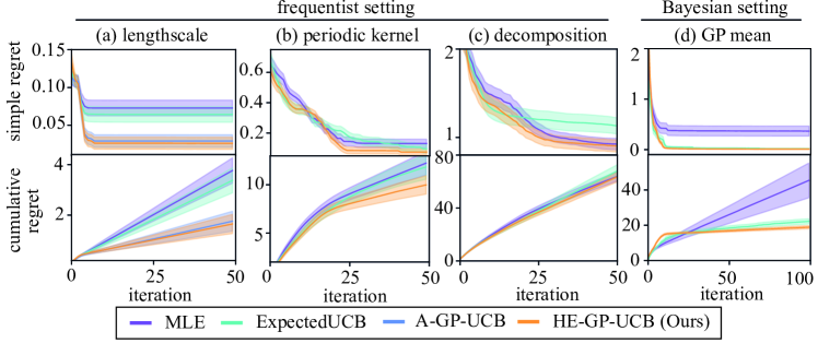
Figure 2: Empirical evaluation of the proposed algorithm and selected baselines. Solid lines represent mean values and shaded areas are standard errors. The results are over 50 seeds for a), b) and d), and 100 seeds for c).

We now empirically evaluate our proposed algorithm. We conduct the evaluation on multiple toy problems, where each time we are given some number of candidate hyperparameter values. The first baseline we compare against is the MLE, which simply selects the hyperparameter value that produces a model with the highest marginal likelihood, i.e. $u_{t}=\arg\max_{u\in U}p(\mathcal{D}|u)$ and then optimises the UCB function $\textrm{UCB}_{t}^{u_{t}}(\bm{x})$ produced by that model. Another baseline is ExpectedUCB, which maximises the expected UCB function $\mathbb{E}_{u\sim P(u|\mathcal{D})}[\textrm{UCB}_{t}^{u}(\bm{x})]$, where $P(u)=\frac{1}{|U|}$. On the experiments with unknown lengthscales, we also compare with A-GP-UCB method of Berkenkamp et al. (2019). We show cumulative regret and simple (best) regret plots in Figure 2. See Appendix J for more details on each experiment.

Unknown lengthscale (a) In the first experiment, we use the function proposed by Berkenkamp et al. (2019) (in their Figure 2). This function is very smooth in most of its domain but becomes less smooth around the global optimum. The unknown hyperparameter in this case is the lengthscale with the candidates being [0.3, 0.4, 0.5, 0.7, 1.0]. While MLE tends to opt for the long lengthscale due to smoothness, ours selects short ones. Both HE-GP-UCB and A-GP-UCB perform very similarly and outperform other baselines.

Unknown period (b) We use a 1-dimensional periodic function consisting of four distinct intervals, which are repeated two times within the domain, see Figure 4, resulting in a function with a period of 1. Each of the intervals, however, contains a sine wave with a much shorter period and as such, the MLE often favoured an incorrect period value. It was less likely for HE-GP-UCB to be misled towards the wrong period value and as such it achieved lower regret.

Unknown decomposition (c) We use the 3-dimensional function proposed by Ziomek & Bou-Ammar (2023) (in their Appendix C). This function locally appears to be fully additive, but the global optimum lies in the region where the first two dimensions are not separable. We use the kernel of form $k(\bm{x},\bm{x}^{\prime})=\sum_{c\in g}k_{c}(\bm{x}_{[c]},\bm{x}^{\prime}_{[c]})$, where $\bm{x}_{[c]}$ selects only the dimensions in set $c$ and $g$ is the unknown hyperparameter. We use different decompositions as candidate hyperparameter values detailed in Appendix J.3. HE-GP-UCB was on average quicker in realising that the first two dimensions are inseparable and thus it performs better in the beginning before other methods can catch up to it.

Unknown GP mean (d) Finally, we also run an experiment in the Bayesian setting. Here the black-box function is a sample from a GP prior with an RBF kernel and a mean function that is zero everywhere, except for certain regions forming ”hills” (see Figure 6 for a graphical depiction). One of those hills is higher than the others and the number of that highest hill is the unknown hyperparameter. We can see that ExpectedUCB performs much better than MLE due to increased exploration caused by not committing to any one specific model. However, HE-GP-UCB still outperforms ExpectedUCB as it explores the function enough by being doubly optimistic and then rejects the incorrect models.

8 Conclusions

Within this paper, we managed to propose the first no-regret algorithm capable of conducting BO with unknown hyperparameters of arbitrary form. We provided a regret bound in both frequentist and Bayesian settings and we also showed how our algorithm can be easily extended to handle adversarially robust BO. We empirically evaluated our algorithm and showed that there are cases, where it can outperform the typically used MLE.

One limitation of our work is that it assumes that the set of candidate hyperparameter values is finite. As explained before, proving convergence with an infinite number of candidates is impossible without stronger assumptions. However, it might be possible to devise a more practical version of our algorithm, which would automatically generate a number of discrete candidates. It could thus handle the case in which there are infinitely many possible hyperparameter values. This constitutes a promising direction of future work.

Appendix A Discussion on Master Algorithms

Within this section we discuss issues that make prevent us from simply applying Master algorithms from the bandit community to our problem setting. We dedicate each of the subsections below to a particular Master algorithm.

A.1 CORRAL

The popular CORRAL algorithm (Agarwal et al., 2017) is a master algorithm designed for an adversarial setting. However, the proof of its regret bound relies on bounding the difference between the regret of the actually selected algorithm and the one of the well-specified algorithm. Applying CORRAL to BO will thus produce a linear bound similar to that of Hoffman et al. (2011), as even though this difference can be sublinear, the regret of the well-specified algorithm depends on the variance at the point it is suggesting and if the point actually chosen by the master algorithm is not that one suggested by the well-specified algorithm, this variance might not decrease and as such the algorithm will not have the no-regret property.

A.2 Regret Balancing

Regret balancing (Abbasi-Yadkori et al., 2020; Pacchiano et al., 2020) is another popular strategy for designing master algorithms. However, it only works if all base algorithms have regret bounds growing equally fast with a number of iterations $T$, which might not be the case in our problem setting. For example, this will not be the case when selecting the decompositions the information gain and thus regret grows differently depending on the decomposition as shown by Rolland et al. (2018).

A.3 Feature Selection in Linear bandits

Moradipari et al. (2022) proposed FS-SCB algorithm, which solves the linear bandits problem with unknown features. Their regret bound depends on the number of dimensions of the feature vector and as such cannot be directly extended to the kernelised case, where feature vectors are possibly infinitely dimensional. Their algorithm is a modification of SCB algorithm of Foster & Rakhlin (2020), which in the kernelised setting achieves the same regret rate $\mathcal{O}(T^{3/4})$ regardless of the kernel function, which is worse than the kernel-dependent regret rate of GP-UCB. As such even if it is possible to kernelise FS-SCB, it would most likely achieve the same kernel-independent scaling, which would be suboptimal compared to existing kernel-dependnent bounds in BO literature.

Appendix B Assumption in continuous Bayesian case

Assumption B.1.

Let $X\subset[0,r]^{d}$ be a compact and convex set, where $r>0$. Assume that the kernel $k^{u^{*}}$ satisfies the following condition on the derivatives of a sample path $f$. There exist constants $a,b>0$ such that,

$$P\left(\sup_{x\in X}\left\lvert\frac{\partial f}{\partial x_{j}}\right\rvert>L\right)\leq a\exp\left(-\frac{L^{2}}{b}\right),$$

for $j\in[d]$, where $[d]=\{1,\ldots,d\}$.

Appendix C Proof of Theorem 4.1

See 4.1

Proof.

Observe that by union bound Theorem 3.1 and Lemma 5.1 hold together with probability at least $1-\delta_{A}-\delta_{B}$. We choose $\delta_{A}=\delta_{B}=\frac{\delta}{2}$. We will prove the regret bound, assuming the probabilistic statements in Theorem 3.1 and Lemma 5.1 hold, and as such the resulting bound holds with probability at least $1-\delta$.

Preservation of $u^{*}$ We first look at the sum of error terms for the true hyperparameter value, when line 10 is executed at some iteration $t$:

$$\left|\sum_{i\in S^{u^{*}}_{t}}\eta_{t}\right|=\left|\sum_{i\in S^{u^{*}}_{t}}\left(y_{t}-f(\bm{x}_{t})+f(\bm{x}_{t})-\mu^{*}_{t-1}(\bm{x}_{t})\right)\right|$$

$$\leq\left|\sum_{i\in S^{u^{*}}_{t}}\epsilon_{t}\right|+\sum_{i\in S^{u^{*}}_{t}}\left|f(\bm{x}_{t})-\mu^{*}_{t-1}(\bm{x}_{t})\right|$$

$$\leq\sqrt{\xi_{t}|S^{u^{*}}_{t}|}+\sum_{i\in S^{u^{*}}_{t}}\beta_{i}^{u^{*}}\sigma_{i}^{u}(\bm{x}_{i}),$$

where the last inequality is due to Theorem 3.1 and Lemma 5.1. As such the condition of the if statement always evaluates to false and $u^{*}\in U_{t}$ for any $t\geq 0$.

Bound on simple regret If $u^{*}\in U_{t-1}$, we trivially have:

$$f(\bm{x}^{*})\leq\mu_{t-1}^{u^{*}}(\bm{x}^{*})+\beta_{t}^{u^{*}}\sigma^{u^{*}}_{t-1}(\bm{x}^{*})$$

$$\leq\max_{\bm{x}_{t}\in\mathcal{X}}\max_{u\in U_{t}}\mu_{t-1}^{u}(\bm{x}_{t})+\beta^{u^{*}}_{t}\sigma_{t-1}^{u}(\bm{x}_{t}).$$ (3)

For simplicity we will write $\mu_{t-1}^{+}=\mu_{t-1}^{u_{t}}$ and $\sigma_{t-1}^{+}=\sigma_{t-1}^{u_{t}}$. Let us now define the error of the lower bound at time $t$ and point $\bm{x}_{t}$ as follows:

$$e_{t}(\bm{x}_{t})=f(\bm{x}_{t})-\left(\mu^{+}_{t-1}(\bm{x}_{t})-\beta^{+}_{t}\sigma^{+}_{t-1}(\bm{x}_{t})\right)$$ (4)

$$=y_{t}-\epsilon_{t}-\left(\mu^{+}_{t-1}(\bm{x}_{t})-\beta^{+}_{t}\sigma^{+}_{t-1}(\bm{x}_{t})\right)$$

$$=\eta_{t}-\epsilon_{t}+\beta^{+}_{t}\sigma^{+}_{t-1}(\bm{x}_{t})$$

Let us look at the instantaneous regret. Combining Inequality 3 and Equation 4, we get:

$$r_{t}=f(\bm{x}^{*})-f(\bm{x}_{t})$$

$$\leq\mu^{+}_{t-1}(\bm{x}_{t})+\beta^{+}_{t}\sigma^{+}_{t-1}(\bm{x}_{t})$$

$$-\mu^{+}_{t-1}(\bm{x}_{t})+\beta^{+}_{t}\sigma^{+}_{t-1}(\bm{x}_{t})-e_{t}(\bm{x}_{t})$$

$$\leq 2\beta^{+}_{t}\sigma^{+}_{t-1}(\bm{x}_{t})-e_{t}(\bm{x}_{t})=-\eta_{t}+\epsilon_{t}+\beta^{+}_{t}\sigma^{+}_{t-1}(\bm{x}_{t}).$$ (5)

Bound on cumulative regret Let us define $\mathcal{C}$ to be the set of ”critical” iterations as below:

$$\mathcal{C}=\left\{t\geq 1:\left|\sum_{i\in S^{u_{t}}}\eta_{i}\right|>\sqrt{\xi_{t}|S^{u_{t}}|}+\sum_{i\in S^{u_{t}}}\beta^{u_{t}}_{i}\sigma_{i}^{u_{t}}(\bm{x}_{i})\right\}$$

Notice that for each $t\in\mathcal{C}$, we will discard one hyperparameter value and as such $|\mathcal{C}|\leq|U|$. On those iterations, we can possibly suffer as high of regret as possible, that is for $t\in\mathcal{C}$ we have $r_{t}\leq 2|f(\bm{x})|_{\infty}\leq 2|f(\bm{x})|_{k^{u^{*}}}\leq 2B$. Using Equation 5, we thus see that the cumulative regret will be bounded as follows:

$$R_{T}\leq\sum_{t\in\mathcal{C}}r_{t}+\sum_{t\notin\mathcal{C}}r_{t}$$

$$\leq 2|U|B-\sum_{t\notin\mathcal{C}}\eta_{t}+\sum_{t\notin\mathcal{C}}\epsilon_{t}+\sum_{t\notin\mathcal{C}}\beta^{+}_{t}\sigma^{+}_{t-1}(\bm{x}_{t})$$

$$=2|U|B+\sum_{t\notin\mathcal{C}}\beta^{+}_{t}\sigma^{+}_{t-1}(\bm{x}_{t})+\sum_{u\in U}\sum_{t\in S^{u}_{T}\setminus\mathcal{C}}\left(\epsilon_{t}-\eta_{t}\right)$$ (6)

When it comes to the terms $\eta_{t}$, observe that if $t\notin\mathcal{C}$ the if statement in line 10 never evaluated to true. For each $u\in U$ we thus have:

$$\sum_{u\in U}\sum_{t\in S^{u}_{T}\setminus\mathcal{C}}-\eta_{t}\leq\sum_{u\in U}\sqrt{\xi_{T}|S^{u}_{T}|}+\sum_{u\in U}\sum_{t\in S^{u}_{T}\setminus\mathcal{C}}\beta^{u}_{t}\sigma_{t}^{u}(\bm{x}_{i}).$$ (7)

Due to Lemma 5.1, we have:

$$\sum_{u\in U}\sum_{t\in S^{u}_{T}\setminus\mathcal{C}}\epsilon_{t}=\sum_{u\in U;u\neq u^{*}}\sum_{t\in S^{u}_{T}\setminus\mathcal{C}}\epsilon_{t}+\sum_{t\in S^{u^{*}}_{T}}\epsilon_{t}$$

$$\leq\sqrt{\xi_{T}|S^{u^{*}}_{T}|}+\sum_{u\in U;u\neq u^{*}}\sqrt{\xi_{T}|S^{u}_{T}\setminus\mathcal{C}|}\leq\sum_{u\in U}\sqrt{\xi_{T}|S^{u}_{T}|}.$$ (8)

Combining Inequality 7 with Inequality 8 and plugging in to Inequality 6:

$$R_{T}\leq 2|U|B+2\sum_{u\in U}\sqrt{\xi_{T}|S^{u}_{T}|}+2\sum_{t\notin\mathcal{C}}\beta^{+}_{t}\sigma^{+}_{t-1}(\bm{x}_{t}).$$ (9)

Dealing with $|S^{u}_{T}|$ Applying Lemma 5.2 to Inequality 9 we get:

$$R_{T}\leq 2|U|B+2\sqrt{|U|\xi_{T}T}+2\sum_{t\notin\mathcal{C}}\beta^{+}_{t}\sigma^{+}_{t-1}(\bm{x}_{t}).$$ (10)

Expressing bound in terms of MIG Applying Lemma 5.3 to Equation 10, we get:

$$R_{T}\leq 2|U|B+2\sqrt{|U|\xi_{T}T}+2\beta_{T}\sqrt{CT|U|\gamma_{T}}$$

∎

Appendix D Proof of Theorem 4.2

See 4.2

Proof.

We consider two cases.

If $|\mathcal{X}|<\infty$

By union bound Theorem 3.1, Lemma 5.1 hold together with probability at least $1-\delta_{A}-\delta_{B}$ and we choose $\delta_{A}=\delta_{B}=\delta_{C}=\frac{\delta}{2}$. Since confidence intervals are valid and noise is bounded then $u^{*}\in U_{t}$ for any $t\geq 0$ and we obtain the instantaneous regret bound $r_{t}\leq\epsilon_{t}-\eta_{t}+\beta^{+}_{t}\sigma^{+}_{t-1}(\bm{x}_{t})$ by the same argument as in frequentist case. Now we have that for $t\in\mathcal{C}$, the instant regret has bound $r_{t}\leq 2B$ (due to Lemma 5.4). Thus the cumulative regret bound in 9 becomes:

$$R_{T}\leq 2|U|B+2\sum_{u\in U}\sqrt{\xi_{T}|S^{u}_{T}|}+2\sum_{t\notin\mathcal{C}}\beta_{t}\sigma^{+}_{t-1}(\bm{x}_{t}).$$

All the remaining steps are the same as in the frequentist case.

If $|\mathcal{X}|=\infty$

By union bound Theorem 3.2 and Lemma 5.1 hold together with probability at least $1-\delta_{A}-\delta_{B}$ and we choose $\delta_{A}=\delta_{B}=\frac{\delta}{2}$. Since confidence intervals are valid for the selected points $\{\bm{x}_{t}\}_{t=1}^{T}$ and noise is bounded then $u^{*}\in U_{t}$ for any $t\geq 0$ by the same argument as in the frequentist case. However, the instantaneous regret bound will change as we rely on Theorem 3.2 instead of 3.1. As $u^{*}\in U_{t-1}$, we have:

$$f(\bm{x}^{*})\leq\mu_{t-1}^{u^{*}}([\bm{x}^{*}]_{t})+\beta^{u^{*}}_{t}\sigma^{u^{*}}_{t-1}([\bm{x}^{*}]_{t})+\frac{1}{t^{2}}$$

$$\leq\max_{\bm{x}_{t}\in\mathcal{X}}\max_{u\in U_{t}}\mu_{t-1}^{u}(\bm{x}_{t})+\beta^{u}_{t}\sigma_{t-1}^{u}(\bm{x}_{t})+\frac{1}{t^{2}}.$$

As such, the instantaneous regret bound will be $r_{t}\leq\epsilon_{t}-\eta_{t}+\beta^{+}_{t}\sigma^{+}_{t-1}(\bm{x}_{t})+\frac{1}{t^{2}}$. The rest of the steps follows the frequentist case, with the exception of bounding the regret on iterations $t\in\mathcal{C}$, where we obtain the same bound as in the case $|\mathcal{X}|<\infty$. This yields the final regret bound of:

$$R_{T}\leq 2|U|B+2\sqrt{|U|\xi_{T}T}+2\beta_{T}\sqrt{CT|U|\gamma_{T}}+\sum_{t=1}^{T}\frac{1}{t^{2}}\leq 2|U|B+2\sqrt{|U|\xi_{T}T}+2\beta_{T}\sqrt{CT|U|\gamma_{T}}+\frac{\pi}{6}$$

∎

Appendix E Proof of Lemma 5.1

See 5.1

Proof.

Let us consider some fixed $u\in U$. Let us define a new set of i.i.d. random variables $v_{i}$ for $i=1,\dots,T$, where each of them follows the same $R$-subgaussian distribution as the noise. Since $v_{i}$ is $R$-subgaussian, for any $0<n\leq T$ we have:

$$P\left(\left|\sum_{i=1}^{n}v_{i}\right|\geq\sqrt{An}\right)\leq 2\exp\left(\frac{-An}{2R^{2}n}\right)=2\exp\left(\frac{-A}{2R^{2}}\right),$$

which is a well-known result in the literature (e.g. see Corollary 5.5 in Lattimore & Szepesvári (2020)). Let us sample each $v_{i}$ for $i=1,\dots,T$ before the experiment starts and let them be a hidden state of the environment. Whenever for the current iteration $t$, we have that the set $S_{t-1}^{u}$ is expanded, we set the noise of that iteration as $\epsilon_{t}=v_{i}$, where $i=|S_{t}^{u}|$. Such a constructed noise must have the same distribution as the original noise. For each $i=1,\dots,T$, let us now define the event $E_{n}$ as:

$$E_{n}:\quad\left|\sum_{i=1}^{n}v_{i}\right|>\sqrt{\xi_{n}n}.$$

We now have:

$$P\left(\exists_{t=1,\dots,T}\left|\sum_{n\in S_{t}^{u}}\epsilon_{n}\right|>\sqrt{\xi_{n}|S_{t}^{u}|}\right)=P\left(\bigcup_{n=1}^{|S_{T}^{u}|}E_{n}\right)\leq P\left(\bigcup_{n=1}^{T}E_{n}\right)$$

$$\leq\sum_{n=1}^{T}P\left(E_{n}\right)\leq 2\sum_{t=1}^{T}\exp\left(\frac{-\xi_{t}}{2R^{2}}\right)=\sum_{t=1}^{T}\frac{6\delta_{B}}{|U|\pi^{2}t^{2}}=\frac{\delta_{B}}{|U|},$$

where the first inequality is due to the fact that $\bigcup_{n=1}^{|S_{T}^{u}|}E_{n}\subseteq\bigcup_{n=1}^{T}E_{n}$ as $|S_{T}^{u}|\leq T$. We finish the proof by taking a union bound over all $u\in U$. ∎

Appendix F Proof of Lemma 5.2

See 5.2

Proof.

We are interested in solving the optimisation problem:

$$\max_{\bm{x}\in\mathbb{R}^{|U|}}\sum_{u\in U}\sqrt{x_{u}}$$ (11)

$$\textrm{s.t. }\sum_{u\in U}x_{u}=T\qquad\forall_{u\in U}\,0\leq x_{u}\leq|U|$$

We will prove the solution is $x_{u}=\frac{T}{|U|}$ for each $u\in U$ and thus optimal value is $\sqrt{|U|T}$. This proves the statement by identifying $x_{u}=|S^{u}_{T}|$. Note that $|S^{u}_{T}|$ can only take discrete values from $\{1,\dots,|U|\}$. We consider relaxation of this problem and as such the optimum value we find must be at least as large as for the original problem. We will prove by induction that the solution to Problem 11 is $x_{u}=\frac{T}{|U|}$ or each $u\in U$. Consider the case when $|U|=2$. Let $v\in U$, then the function we want to optimise is:

$$f(x_{v})=\sqrt{x_{v}}+\sqrt{T-x_{v}},$$

and by taking its derivative and setting it to zero we get $x_{v}^{*}=\frac{T}{2}$. Assuming that for $|U|=n$ the statement holds, we will prove it must also hold for $|U|=n+1$. In the latter case the function we want to optimise is:

$$f(x_{v})=\sqrt{x_{v}}+\sum_{u\in U;u\neq v}\sqrt{x_{u}}=\sqrt{x_{v}}+\sum_{u\in U;u\neq v}\sqrt{\frac{T-x_{v}}{|U|-1}},$$

where the second equality is true as if the induction hypothesis holds we must have that the solution to $\sum_{u\in U;u\neq v}\sqrt{x_{u}}$ subject to constraint $\sum_{u\in U;u\neq v}=T-x_{v}$ is $x_{u}^{*}=\frac{T-x_{v}}{|U\setminus\{x_{v}\}|}=\frac{T-x_{v}}{|U|-1}$ for all $u\in U;u\neq v$. Again, taking derivative of $f(x_{v})$ and setting it to zero gives $x_{v}^{*}=\frac{T}{|U|}$ and thus $x_{u}^{*}=\frac{T-\frac{T}{|U|}}{|U|-1}=\frac{T}{|U|}$ for all remaining $u\in U;u\neq v$. ∎

Appendix G Proof of Lemma 5.3

See 5.3

Proof.

Firstly, observe that due to Cauchy-Schwarz we have:

$$\sum_{t\notin\mathcal{C}}\beta_{t}^{+}\sigma^{+}_{t-1}(\bm{x}_{t})\leq\beta_{T}\sqrt{(T-|\mathcal{C}|)\sum_{t\notin\mathcal{C}}(\sigma^{+}_{t-1})^{2}(\bm{x}_{t})}\leq\beta_{T}\sqrt{T\sum_{u\in U}\sum_{\begin{subarray}{c}t\notin\mathcal{C}\\ u_{t}=u\end{subarray}}(\sigma^{u}_{t-1})^{2}(\bm{x}_{t})},$$ (12)

where $\beta_{T}=\max_{u\in U}\beta^{u}_{T}$. We will need to introduce some new notation. For some set of inputs $A\subset\mathcal{X}$, let us define:

$$(\sigma^{u}_{A})^{2}(\bm{x})=k(\bm{x},\bm{x})^{u}-\bm{k}^{u}_{A}(\bm{x})^{T}(K^{u}_{A}+\sigma^{2}\mathcal{I})^{-1}\bm{k}^{u}_{A}(\bm{x}),$$

where $K^{u^{*}}_{A}=[k^{u^{*}}(\bm{x},\bm{x}^{\prime})]_{\bm{x},\bm{x}^{\prime}\in A}$ and $\bm{k}^{u^{*}}_{A}=[k^{u^{*}}(\bm{x},\bm{x}^{\prime})]_{\bm{x}^{\prime}\in A}$ Notice that under such notation $\sigma^{u}_{t-1}=\sigma^{u}_{X_{t-1}}$, where $X_{t-1}=\{\bm{x}_{i}\}_{i=1}^{t-1}$. Let us define $A^{u}_{t-1}=\{\bm{x}_{i}:1\leq i\leq t-1,u_{t}=u\}$ to be the set of points queried when $u_{t}=u$. For any two sets $S,S^{\prime}$ such that $S^{\prime}\subseteq S$ we have $\sigma^{u}_{S^{\prime}}(\bm{x})\leq\sigma^{u}_{S}(\bm{x})$ for all $\bm{x}\in\mathcal{X}$. As $A^{u}_{t-1}\subseteq X_{t}$, we have:

$$(\sigma^{+}_{t-1})^{2}(\bm{x}_{t})=(\sigma^{u}_{X_{t}})^{2}(\bm{x}_{t})\leq(\sigma^{u}_{A^{u}_{t-1}})^{2}(\bm{x}_{t})\leq C\log(1+R^{-2}(\sigma^{u}_{A_{t-1}^{u}}(\bm{x}))^{2}),$$

for some $C$ (depending on $R$), where the last inequality is true due to the same reasoning as in the proof of Lemma 5.4 in (Srinivas et al., 2010). Applying this fact to Inequality 12 gives:

$$\beta_{T}\sqrt{T\sum_{u\in U}\sum_{\begin{subarray}{c}t\notin\mathcal{C}\\ u_{t}=u\end{subarray}}(\sigma^{u}_{t-1})^{2}(\bm{x}_{t})}\leq\beta_{T}\sqrt{CT\sum_{u\in U}\sum_{\begin{subarray}{c}t\notin\mathcal{C}\\ u_{t}=u\end{subarray}}\log(1+R^{-2}(\sigma^{u}_{A_{t-1}^{u}}(\bm{x}))^{2})}$$

$$=\beta_{T}\sqrt{CT\sum_{u\in U}\gamma_{|A^{u}_{t-1}|}^{u}}\leq\beta_{T}\sqrt{CT|U|\gamma_{T}}$$

where the penultimate equality follows from Lemma 5.3 from (Srinivas et al., 2010). ∎

Appendix H Proof of Lemma 5.4

See 5.4

Proof.

We will consider two cases, depending on cardinality of $|\mathcal{X}|$.

If $|\mathcal{X}|<\infty$

Note that if event of Theorem 3.1 holds, then at $t=1$, we have that for all $\bm{x}\in\mathcal{X}$:

$$|f(\bm{x})-\mu_{1}(\bm{x})|\leq\beta_{1}\sigma_{0}(\bm{x})\leq\beta_{1}k(\bm{x},\bm{x})\leq\beta_{1}$$

As such:

$$\max_{\bm{x}\in\mathcal{X}}|f(\bm{x})|\leq\beta_{1}+\max_{\bm{x}\in\mathcal{X}}|\mu_{0}(\bm{x})|=B,$$

which completes the proof.

If $|\mathcal{X}|=\infty$

Note that if event of Theorem 3.2 holds, then at $t=1$, we have that for all $\bm{x}\in\mathcal{X}$:

$$|f(\bm{x})-\mu_{1}([\bm{x})]_{1}|\leq\beta_{1}\sigma_{0}([\bm{x}]_{1})+1\leq\beta_{1}k([\bm{x}]_{1},[\bm{x}]_{1})+1\leq\beta_{1}+1$$

As such:

$$\sup_{\bm{x}\in\mathcal{X}}|f(\bm{x})|\leq\beta_{1}+\max_{\bm{x}\in D_{t}}|\mu_{0}(\bm{x})|+1\leq\beta_{1}+\sup_{\bm{x}\in\mathcal{X}}|\mu_{0}(\bm{x})|+1=B,$$

which completes the proof.

∎

Appendix I Adversarially Robust Optimisation

Algorithm 2 StableOpt with Hyperparameter Elimination
(HE-StableOpt)

0:  a set of possible hyperparameters values $U$; confidence parameters $\{\xi_{t}\}_{t=1}^{T}$ and $\{\{\beta^{u}_{t}\}_{t=1}^{T}\}_{u\in U}$; stability $\epsilon$, distance function $d(\cdot,\cdot)$

1:  Set $\mathcal{D}_{0}=\emptyset$, $U_{0}=U$, $S^{u}=\emptyset$, $\hat{S}^{u}=\emptyset$ for each $u\in U$

2:  for $t=1,\dots,T$ do

3:     for $u\in U_{t-1}$ do

4:        Fit a GP $(\mu^{u}_{t-1}(\bm{x}),\sigma^{u}_{t-1}(\bm{x}))$ to $\mathcal{D}_{t-1}$

5:        Set $\textrm{UCB}_{t-1}^{u}(\bm{x})=\mu^{u}_{t-1}(\bm{x})+\beta_{t}^{u}\sigma^{u}_{t-1}(\bm{x})$

6:        Set $\textrm{LCB}_{t-1}^{u}(\bm{x})=\mu^{u}_{t-1}(\bm{x})-\beta_{t}^{u}\sigma^{u}_{t-1}(\bm{x})$

7:     end for

8:     Find $\bm{x}_{t},u_{t}=\underset{\bm{x},u\in\mathcal{X}\times U_{t-1}}{\arg\max}\min_{\bm{\delta}\in\Delta_{\epsilon}(\bm{x})}\textrm{UCB}_{t-1}^{u}(\bm{x}+\bm{\delta})$

9:     Find $\bm{\delta}_{t},v_{t}=\underset{\bm{\delta},u\in\Delta_{\epsilon}(\bm{x}_{t})\times U_{t-1}}{\arg\min}\textrm{LCB}_{t-1}^{u}(\bm{x}_{t}+\bm{\delta})$

10:     $S^{u_{t}}_{t}=S^{u_{t}}_{t-1}\cup\{t\}$ and $S^{u}_{t}=S^{u}_{t-1}$ for $u\in U;u\neq u_{t}$

11:     $\hat{S}^{v_{t}}_{t}=\hat{S}^{v_{t}}_{t-1}\cup\{t\}$ and $\hat{S}^{u}_{t}=\hat{S}^{u}_{t-1}$ for $u\in U;u\neq v_{t}$

12:     Query the black-box $y_{t}=f(\bm{x}_{t}+\bm{\delta})$

13:     Set $\mathcal{D}_{t}=\mathcal{D}_{t-1}\cup(\bm{x}_{t}+\bm{\delta}_{t},y_{t})$

14:     Set $\eta_{t}=y_{t}-\mu^{u_{t}}_{t-1}(\bm{x}_{t}+\bm{\delta}_{t})$

15:     Set $\hat{\eta}_{t}=y_{t}-\mu^{v_{t}}_{t-1}(\bm{x}_{t}+\bm{\delta}_{t})$

16:     if $\left|\sum_{i\in S^{u_{t}}_{t}}\eta_{i}\right|>\sqrt{\xi_{t}|S^{u_{t}}_{t}|}+\sum_{i\in S^{u_{t}}_{t}}\beta^{u_{t}}_{i}\sigma_{i}^{u_{t}}(\bm{x}_{i}+\bm{\delta}_{i})$  then

17:        $U_{t}=U_{t-1}\setminus\{u_{t}\}$

18:     end if

19:     if $\left|\sum_{i\in\hat{S}^{v_{t}}_{t}}\hat{\eta}_{i}\right|>\sqrt{\xi_{t}|\hat{S}^{v_{t}}_{t}|}+\sum_{i\in\hat{S}^{v_{t}}_{t}}\beta^{v_{t}}_{i}\sigma_{i}^{v_{t}}(\bm{x}_{i}+\bm{\delta}_{i})$  then

20:        $U_{t}=U_{t-1}\setminus\{v_{t}\}$

21:     end if

22:  end for

See 6.1

Proof.

We start with the frequentist case and then comment on the difference in Bayesian case. Observe that by union bound Theorem 3.1 and Lemma 5.1 hold together with probability at least $1-\delta_{A}-\delta_{B}$. We choose $\delta_{A}=\delta_{B}=\frac{\delta}{2}$. We will prove the regret bound, assuming the probabilistic statements in Theorem 3.1 and Lemma 5.1 hold, and as such the resulting bound holds with probability at least $1-\delta$.

By exactly the same argument as in the proof of Theorem 4.1, we must have that $u^{*}\in U_{t}$ for all $0\leq t\leq T$, with the only difference that $\bm{x}_{t}$ is replaced with $\bm{x}_{t}+\bm{\delta}_{t}$. Let us now look at the instantaneous regret:

$$r_{t}=\max_{\bm{x}\in D}\min_{\bm{\delta}\in\Delta_{\epsilon}(\bm{x})}f(\bm{x}+\bm{\delta})-\min_{\bm{\delta}\in\Delta_{\epsilon}(\bm{x}_{t})}f(\bm{x}_{t}+\bm{\delta})$$

$$\leq\max_{\bm{x}\in D}\min_{\bm{\delta}\in\Delta_{\epsilon}(\bm{x})}\textrm{UCB}^{u^{*}}_{t}(\bm{x}+\bm{\delta})-\min_{\bm{\delta}\in\Delta_{\epsilon}(\bm{x}_{t})}\textrm{LCB}^{u^{*}}_{t}(\bm{x}_{t}+\bm{\delta})$$

$$\leq\textrm{UCB}^{u_{t}}_{t}(\bm{x}_{t}+\bm{\delta}_{t})-\textrm{LCB}^{v_{t}}_{t}(\bm{x}_{t}+\bm{\delta}_{t})$$

$$=\mu^{u_{t}}_{t-1}(\bm{x}_{t}+\bm{\delta}_{t})-y_{t}+\beta^{u_{t}}_{t}\sigma_{t-1}^{u_{t}}(\bm{x}_{t}+\bm{\delta}_{t})-\left(y_{t}-\mu^{v_{t}}_{t-1}(\bm{x}_{t}+\bm{\delta}_{t})-\beta^{v_{t}}_{t}\sigma^{v_{t}}_{t-1}(\bm{x}_{t}+\bm{\delta}_{t})\right)$$

$$=\eta_{t}+\beta^{u_{t}}_{t}\sigma_{t-1}^{u_{t}}(\bm{x}_{t}+\bm{\delta}_{t})+\hat{\eta}_{t}+\beta^{v_{t}}_{t}\sigma^{v_{t}}_{t-1}(\bm{x}_{t}+\bm{\delta}_{t}),$$

where the first inequality is due to Theorem 3.1 and second due to definitions of $\bm{x}_{t}$, $\bm{\delta}_{t}$, $u_{t}$ and $v_{t}$. Similarly as in the proof of Theorem 4.1, we define the set of critical iterations as:

$$\mathcal{C}=\left\{0\leq t\leq T:\left|\sum_{i\in S^{u_{t}}_{t}}\eta_{i}\right|>\sqrt{\xi_{t}|S^{u_{t}}_{t}|}+\sum_{i\in S^{u_{t}}_{t}}\beta^{u_{t}}_{i}\sigma_{i}^{u_{t}}(\bm{x}_{i}+\bm{\delta}_{i})\textrm{ OR }\left|\sum_{i\in\hat{S}^{v_{t}}_{t}}\eta_{i}\right|>\sqrt{\xi_{t}|\hat{S}^{v_{t}}_{t}|}+\sum_{i\in\hat{S}^{v_{t}}_{t}}\beta^{v_{t}}_{i}\sigma_{i}^{v_{t}}(\bm{x}_{i}+\bm{\delta}_{i})\right\}.$$

Notice that we will reject one hyperparameter value for each iteration in $\mathcal{C}$ and as such $|\mathcal{C}|<|U|$. We now look at the cumulative regret:

$$\sum_{t=1}^{T}r_{t}\leq\sum_{t\in\mathcal{C}}r_{t}+\sum_{t\not\in\mathcal{C}}r_{t}\leq 2|U|B+\sum_{t\not\in\mathcal{C}}\eta_{t}+\sum_{t\not\in\mathcal{C}}\beta_{t}\sigma_{t-1}^{u_{t}}(\bm{x}_{t}+\bm{\delta}_{t})+\sum_{t\not\in\mathcal{C}}\hat{\eta}_{t}+\sum_{t\not\in\mathcal{C}}\beta_{t}\sigma^{v_{t}}_{t-1}(\bm{x}_{t}+\bm{\delta}_{t}).$$

Observe that due to definition of $\mathcal{C}$, we have:

$$\sum_{t\not\in\mathcal{C}}\hat{\eta}_{t}=\sum_{u\in U}\sum_{t\in S^{u}_{T}\setminus\mathcal{C}}-\eta_{t}\leq\sum_{u\in U}\sqrt{\xi_{T}|S^{u}_{T}|}+\sum_{u\in U}\sum_{t\in S^{u}_{T}\setminus\mathcal{C}}\beta^{u}_{t}\sigma_{t}^{u}(\bm{x}_{i}+\bm{\delta}_{i})$$

$$\sum_{t\not\in\mathcal{C}}\hat{\eta}_{t}=\sum_{u\in U}\sum_{t\in\hat{S}^{u}_{T}\setminus\mathcal{C}}-\hat{\eta}_{t}\leq\sum_{u\in U}\sqrt{\xi_{T}|\hat{S}^{u}_{T}|}+\sum_{u\in U}\sum_{t\in\hat{S}^{u}_{T}\setminus\mathcal{C}}\beta^{u}_{t}\sigma_{t}^{u}(\bm{x}_{i}+\bm{\delta}_{i}).$$

Continuing with the cumulative regret bound, we get:

$$\sum_{t=1}^{T}r_{t}\leq 2|U|B+\sum_{u\in U}\sqrt{\xi_{T}|S^{u}_{T}|}+2\sum_{t\not\in\mathcal{C}}\beta^{u_{t}}_{t}\sigma_{t-1}^{u_{t}}(\bm{x}_{t}+\bm{\delta}_{t})+\sum_{u\in U}\sqrt{\xi_{T}|\hat{S}^{u}_{T}|}+2\sum_{t\not\in\mathcal{C}}\beta^{v_{t}}_{t}\sigma^{v_{t}}_{t-1}(\bm{x}_{t}+\bm{\delta}_{t}).$$

Applying Lemma 5.2 and 5.3 to the bound above we get:

$$R_{T}=\sum_{t=1}^{T}r_{t}\leq\mathcal{O}\left(|U|B+\sqrt{|U|\xi_{T}T}+\beta_{T}\sqrt{T|U|\gamma_{T}}\right),$$

which finishes the proof in the frequentist case. In the Bayesian case, we rely on Theorem 3.2 instead of Theorem 3.1. The rest of the proof follows in the same manner except that now we have an additional term $\sum_{t\notin C}\frac{1}{t^{2}}\leq\frac{\pi^{2}}{6}$, which just adds a constant without affecting the regret bound. ∎

Appendix J Experimental Details

We have implemented the code based on PyTorch (Paszke et al., 2019), GPyTorch (Gardner et al., 2018), BoTorch (Balandat et al., 2020). To compute the maximum information gain, we used the implementation in the code https://github.com/kihyukh/aistats2023 (Hong et al., 2023). Our code is ready to review on https://anonymous.4open.science/r/HE-GP-UCB-6868/. We have run our experiments on a MacBook Pro 2019, 2.4 GHz 8-Core Intel Core i9, 64GB 2667 MHz DDR4. For all experiments, we selected $\delta=0.1$.

J.1 Unknown lengthscale

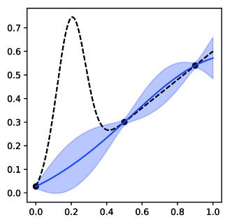
Figure 3: The synthetic function and GP surrogate model with used for unknown lengthscale problem setting.

Figure 3 shows the synthetic function used for the unknown lengthscale problem, firstly introduced in Berkenkamp et al. (2019). We used the following equation to produce this:

$$f(x):=0.6x+0.8\mathcal{N}(x;0.2,0.08)$$ (13)

This function is broadly smooth and has a global linear trend. If the limited data does not contain points from the Gaussian peak, as is the case in Figure 3, MLE opts for the smooth interporation, namely the long lengthscale, and cannot contain the bump within the confidence interval. Thus, misspecified long lengthscale UCB leads to persistently querying at the rightmost point, and will never find the true global maximum at the peak. On the other hand, shorter lengthscale can have a larger confidence interval thus it can find the global maximum. We implemented the A-GP-UCB (Berkenkamp et al., 2019) using their equation (18), and we set $g(t):=t^{0.9}$, following their section 5. Original A-GP-UCB is for continuous hyperparameters, so we use the nearest values from the candidate list instead. We used three uniform i.i.d. samples from the domain $[0,1]$ as the initial samples, then we iterated BO for 50 iterations, and repeated the BO experiments 50 times with different random seeds.

J.2 Unknown period

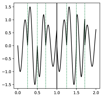
Figure 4: The synthetic function used for the unknown period problem setting.

We use a 1-dimensional periodic function, of which the signal is segmented into four distinct intervals and is repeated two times within the domain, as such:

$$f(x)=\begin{cases}\sin(8\pi(x-1/8)),&\text{if }x<0.25\\ 1.5\sin(28/3\pi),&\text{if }0.25\leq x<0.5\\ 1.2\sin(8\pi(x-11/28)),&\text{if }0.5\leq x<5/7\\ 0.8\sin(8\pi(x-5/7)),&\text{if }5/7\leq x\\ \end{cases}.$$ (14)

The above function is bounded for $[0,1]$, and we repeat the same signal to $[1,2]$ to be periodical. The whole domain is $[0,2]$. We show the plot of the function in Figure 4. This function is misleading, as it has four local periodic sine waves. Locally fitting the period hyperparameter to each of sine waves will never produce the true period of 1.

We generate the true hyperparameter by fitting a GP using maximum likelihood with a large number of uniform samples from the whole domain $[0,2]$. The other hyperparameter candidates are produced by fitting a GP with maximum likelihood for each of the local sine waves. We used five uniform i.i.d. samples from the domain $[0,2]$ as the initial samples, then we iterate BO for 50 iterations, and repeat the BO experiments 50 times with different random seeds.

J.3 Unknown decomposition

We used the three-dimensional function initially proposed by (Ziomek & Bou-Ammar, 2023), which we show in Figure 5. Although the function is three-dimensional, the last dimension is redundant and thus we only show the heatplot with respect to the first two dimensions. We use a kernel of form $k(\bm{x},\bm{x}^{\prime})=\sum_{c\in g}k_{c}(\bm{x}_{[c]},\bm{x}^{\prime}_{[c]})$, with candidates for hyperparameter $g$ being $U=\{((1),(2),(3)),((1,2),(3)),((1),(2,3)),((2),(1,3))\}$ with the second hyperparameter being the true one. We run 100 seeds for each baseline and each seed consisted of 50 iterations.

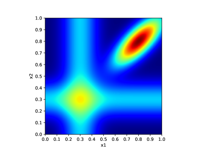
Figure 5: Heatplot of the function used for unknown decomposition problem setting. The function used is actually three-dimensional, but as the last dimension $x3$ is redundant, the function value does not change even when $x3$ changes. The function locally appears as if it could be written as an additive decomposition, however, this is not possible due to the correlated mode in the top right corner.

J.4 Unknown GP mean

We use the mean function shown in Figure 6, where there are ten ”hills” and one ”hill” is higher than others. The number of the highest hill is the unknown hyperparameter. The candidate set is $U=\{1,2,3,4,5,6,7,8,9,10,-1\}$, where $-1$ corresponds to none of the hills being the tallest. For each seed, we sample a new black-box function from the GP with the aforementioned mean function and an RBF kernel. We run 50 seeds for each baseline and each seed for 100 iterations. Each baseline was run with the same seeds and as such, with the same set of 50 random, black-box functions.

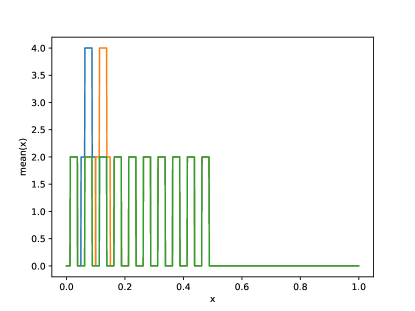
Figure 6: Plot of the mean function used for the unknown GP mean problem setting. Blue and orange curves show prior means corresponding to the second and third hill being tallest. The green curve shows the case, where none of the hills is tallest.

References

- Abbasi-Yadkori et al. (2020) Abbasi-Yadkori, Y., Pacchiano, A., and Phan, M. Regret balancing for bandit and RL model selection. arXiv preprint arXiv:2006.05491, 2020.
- Agarwal et al. (2017) Agarwal, A., Luo, H., Neyshabur, B., and Schapire, R. E. Corralling a band of bandit algorithms. In Conference on Learning Theory, pp. 12–38. PMLR, 2017.
- Bachoc (2013) Bachoc, F. Cross validation and maximum likelihood estimations of hyper-parameters of Gaussian processes with model misspecification. Computational Statistics & Data Analysis, 66:55–69, 2013.
- Balandat et al. (2020) Balandat, M., Karrer, B., Jiang, D., Daulton, S., Letham, B., Wilson, A. G., and Bakshy, E. BoTorch: a framework for efficient Monte-Carlo Bayesian optimization. Advances in neural information processing systems, 33:21524–21538, 2020.
- Berkenkamp et al. (2019) Berkenkamp, F., Schoellig, A. P., and Krause, A. No-regret Bayesian optimization with unknown hyperparameters. The Journal of Machine Learning Research, 20(1):1868–1891, 2019.
- Bogunovic et al. (2018) Bogunovic, I., Scarlett, J., Jegelka, S., and Cevher, V. Adversarially robust optimization with Gaussian processes. Advances in neural information processing systems, 31, 2018.
- Bull (2011) Bull, A. D. Convergence rates of efficient global optimization algorithms. Journal of Machine Learning Research, 12(10), 2011.
- Chowdhury & Gopalan (2017) Chowdhury, S. R. and Gopalan, A. On kernelized multi-armed bandits. In International Conference on Machine Learning, pp. 844–853. PMLR, 2017.
- Cowen-Rivers et al. (2022) Cowen-Rivers, A. I., Lyu, W., Tutunov, R., Wang, Z., Grosnit, A., Griffiths, R. R., Maraval, A. M., Jianye, H., Wang, J., Peters, J., et al. HEBO: Pushing the limits of sample-efficient hyper-parameter optimisation. Journal of Artificial Intelligence Research, 74:1269–1349, 2022.
- Foster & Rakhlin (2020) Foster, D. and Rakhlin, A. Beyond UCB: Optimal and efficient contextual bandits with regression oracles. In International Conference on Machine Learning, pp. 3199–3210. PMLR, 2020.
- Gardner et al. (2018) Gardner, J., Pleiss, G., Weinberger, K. Q., Bindel, D., and Wilson, A. G. GPyTorch: Blackbox matrix-matrix Gaussian process inference with GPU acceleration. In Advances in Neural Information Processing Systems, pp. 7576–7586, 2018.
- Garnett (2023) Garnett, R. Bayesian optimization. Cambridge University Press, 2023.
- Grosnit et al. (2022) Grosnit, A., Malherbe, C., Tutunov, R., Wan, X., Wang, J., and Ammar, H. B. BOiLS: Bayesian optimisation for logic synthesis. In 2022 Design, Automation & Test in Europe Conference & Exhibition (DATE), pp. 1193–1196. IEEE, 2022.
- Ha et al. (2023) Ha, H., Nguyen, V., Zhang, H., and Hengel, A. v. d. Provably efficient Bayesian optimization with unbiased Gaussian process hyperparameter estimation. arXiv preprint arXiv:2306.06844, 2023.
- Hoffman et al. (2011) Hoffman, M., Brochu, E., and de Freitas, N. Portfolio allocation for Bayesian optimization. In Proceedings of the Twenty-Seventh Conference on Uncertainty in Artificial Intelligence, pp. 327–336, 2011.
- Hong et al. (2023) Hong, K., Li, Y., and Tewari, A. An optimization-based algorithm for non-stationary kernel bandits without prior knowledge. In International Conference on Artificial Intelligence and Statistics, pp. 3048–3085. PMLR, 2023.
- Hvarfner et al. (2023) Hvarfner, C., Hellsten, E. O., Hutter, F., and Nardi, L. Self-correcting Bayesian optimization through Bayesian active learning. In Thirty-seventh Conference on Neural Information Processing Systems, 2023.
- Kandasamy et al. (2015) Kandasamy, K., Schneider, J., and Póczos, B. High dimensional Bayesian optimisation and bandits via additive models. In International conference on machine learning, pp. 295–304. PMLR, 2015.
- Khan et al. (2023) Khan, A., Cowen-Rivers, A. I., Grosnit, A., Robert, P. A., Greiff, V., Smorodina, E., Rawat, P., Akbar, R., Dreczkowski, K., Tutunov, R., et al. Toward real-world automated antibody design with combinatorial Bayesian optimization. Cell Reports Methods, 3(1), 2023.
- Lattimore & Szepesvári (2020) Lattimore, T. and Szepesvári, C. Bandit algorithms. Cambridge University Press, 2020.
- Moradipari et al. (2022) Moradipari, A., Turan, B., Abbasi-Yadkori, Y., Alizadeh, M., and Ghavamzadeh, M. Feature and parameter selection in stochastic linear bandits. In International Conference on Machine Learning, pp. 15927–15958. PMLR, 2022.
- Pacchiano et al. (2020) Pacchiano, A., Dann, C., Gentile, C., and Bartlett, P. Regret bound balancing and elimination for model selection in bandits and RL. arXiv preprint arXiv:2012.13045, 2020.
- Paszke et al. (2019) Paszke, A., Gross, S., Massa, F., Lerer, A., Bradbury, J., Chanan, G., Killeen, T., Lin, Z., Gimelshein, N., and Antiga, L. PyTorch: An imperative style, high-performance deep learning library. Advances in neural information processing systems, 32, 2019.
- Rolland et al. (2018) Rolland, P., Scarlett, J., Bogunovic, I., and Cevher, V. High-dimensional Bayesian optimization via additive models with overlapping groups. In International conference on artificial intelligence and statistics, pp. 298–307. PMLR, 2018.
- Srinivas et al. (2010) Srinivas, N., Krause, A., Kakade, S. M., and Seeger, M. Gaussian process optimization in the bandit setting: No regret and experimental design. In International Conference on International Conference on Machine Learning, pp. 1015–1022, 2010.
- Wang & de Freitas (2014) Wang, Z. and de Freitas, N. Theoretical analysis of Bayesian optimisation with unknown Gaussian process hyper-parameters. arXiv preprint arXiv:1406.7758, 2014.
- Ziomek & Bou-Ammar (2023) Ziomek, J. K. and Bou-Ammar, H. Are random decompositions all we need in high dimensional Bayesian optimisation? In International Conference on Machine Learning, pp. 43347–43368. PMLR, 2023.