Spatial correlations of vortex quantum states

Abstract

We study spatial correlations of vortices in different quantum states or with Bose or Fermi statistics. This is relevant for both optical vortices and condensed-matter ones such as microcavity polaritons, or any platform that can prepare and image fields in space at the few-particle level. While we focus on this particular case for illustration of the formalism, we already reveal unexpected features of spatial condensation whereby bosons exhibit a bimodal distribution of their distances which places them farther apart than fermions in over 40% of the cases, or on the opposite conceal spatial correlations to behave like coherent states. Such experiments upgrade in the laboratory successful techniques in uncontrolled extreme environments (stars and nuclei).

In a statistical theory, when waves interfere, they produce correlations between them. This elementary fact surprisingly escaped notice for centuries despite the unanimous embrace and resounding successes of both wave theory and of statistics. This changed when a young engineer (Hanbury Brown) [1] working on the secret development of the radar for British intelligence, spotted the effect with his naked eyes on oscilloscope traces and used it to create a new type of stellar interferometry [2]. Purcell [3] understood that this counter-intuitive effect—correlations from non-interacting, indeed merely interfering objects—was in fact fully expected from even more fundamental quantum mechanical considerations and extended it to fermions, predicting instead anticorrelations as opposed to bosonic positive correlations. The effect became a powerful tool to measure sizes ranging from the diameters of stars (${10}^{12}\text{\,}\mathrm{cm}$) to high-energy nuclear matter (${10}^{-12}\text{\,}\mathrm{cm}$) [4]. While in radioastronomy, intensity interferometry has been described by Hanbury Brown as “building a steam roller to crack a nut” [1], the technique became indispensable in high-energy physics and nuclear physics [5]. It allowed the first measurement of the radius of interactions for the proton-antiproton process from the amount of correlations of identical pions formed in the nuclear reaction [6]. Since then, it became a central, sometimes only, way to measure sizes and lifetimes of high-energy particles and nuclear reactions [7], being instrumental for instance in the investigation of such extreme forms of matter as the quark-gluon plasma formed in ultrarelativistic nucleus-nucleus collisions [8]. In quantum optics, while the emphasis has been on temporal correlations, technological progress, e.g., with superconducting nanowire single-photon detectors [9], can capture increasingly high-resolution images from single-photon pixelated detectors [10], thus bringing back spatial quantum correlations to the fore of solid-state and condensed-matter physics [11]. In high-energy and nuclear physics, bosonic correlations—bunching of events—are mostly investigated, since fermionic correlations are shadowed by stronger particle interactions (typically, Coulomb repulsion from charged particles). In contrast, low-energy quantum optics became able to control the statistics of photons through their underlying quantum state. Indeed, Glauber understood coherence as the faculty of photons to neutralize their intrinsic Boson correlations [12] to be detected as an uncorrelated (Poisson) stream, which could be understood as the wave-like limit of light where the particle aspect vanishes. At the other extreme, photons can also be made to behave like fermions by exhibiting antibunching [13, 14, 15]. The ability to control, or at least characterize, quantum states from photon correlations resolved spatially could endow spectroscopic techniques with new and considerably enhanced opportunities as compared to their Bose-Einstein interferometry counterpart [5].

Here, we describe correlations of multi-particle quantum states extended in real space (or other related spaces through the appropriate transforms). To keep the discussion simple and to the point, we focus on a particular case that interfaces between optics [16, 17] and condensed matter, namely, vortices [18]. Microcavity polaritons [19], sitting halfway between optics and the solid state, and with a particularly fruitful development of vortices [20, 21], provide but one example of a platform where to pursue the next generation of bosonic interferometry. As the topological cornerstone of 2D quantum fields, vortices are central to many polaritonic breakthroughs [22, 23], from the observation of their BKT phase transitions [24] to, more recently, the realization of the superfluid bucket experiment [25, 26] passing by Rabi-propelled dynamics [27] or quantum turbulence [28]. As quasi-particles which admix both light (photons) and matter (semiconductor electron-hole pairs, or excitons), polaritons have always elicited a quantum-mechanical formulation, in particular as superpositions with a wavefunction $\ket{\psi}\equiv\alpha(t)\ket{1_{a},0_{b}}+\beta(t)\ket{0_{a},1_{b}}$ that entangles a photon (with Bose creation operator ${a^{\dagger}}$) and the exciton vacuum to its Rabi-flop counterpart with one exciton (operator ${b^{\dagger}}$) and no photon. This genuinely quantum-mechanical state was, however, not realized until recently, by direct excitation of a microcavity with quantum light [29, 30]. In all other cases, a product state $\ket{\alpha(t)}_{a}\otimes\ket{\beta(t)}_{b}$ (no entanglement) or something similar (with some amount of squeezing [31, 32, 33] but still within Gaussian states), is realized instead. In such cases, the probability amplitudes of $\ket{\psi}$ become classical-field amplitudes for coherent states of both the photon and exciton fields [34]. Because $\alpha(t)$ and $\beta(t)$ follow the same equations of motion in both interpretations, although these are very different (quantum probabilities or classical-field amplitudes, respectively), there tends to be some confusion as to the exact quantumness involved with polaritons. One of the outcomes of studying spatial correlations of photons emitted by the polariton field will be to provide clear-cut experimental resolves of the central and long-standing question of their quantum character. We also consider fermionic statistics, that can be realized for spatial wavefunction with singlet-spin. Our considerations are not specific neither to polaritons nor to vortices, which merely provide an illustration of the potential of spatial multiphoton correlations.

Quantum mechanics is a wave theory, and at the heart of its formalism lie the eigenmodes of the system being described. Vortices provide a textbook case of basis states for the 2D harmonic oscillator, for which they provide eigenstates of defined angular momentum in terms of the 1D eigenfunctions $\phi_{n}(x)\equiv\big{(}\sqrt{2^{n}n!}\pi^{1\over 4}\big{)}^{-1}e^{-{x^{2}/2}}H_{n}(x)$ with $H_{n}(x)$ the Hermite polynomials with $n\geq 0$ integers and $x$ in units of the single-charge vortex radius. It will be enough for our discussion to consider stationary 2D vortices with $\pm 1$ topological charge, denoted $\ket{\circlearrowleft}$ and $\ket{\circlearrowright}$, with eigenfunctions $\phi_{\circlearrowleft}(\mathbf{r})=\phi_{\circlearrowright}^{*}(\mathbf{r})\equiv\innerproduct{x,y}{\circlearrowleft}=\big{[}\phi_{1}(x)\phi_{0}(y)+i\phi_{0}(x)\phi_{1}(y)\big{]}/\sqrt{2}$. Given the separation of variables and linearity of quantum mechanics, we can actually develop the formalism for one variable only and keep our discussion one-dimensional. This will be at no loss of generality but with great simplifications of the notations. In the second quantization formalism, the family of $n$-particle density distributions is written in terms of a field operator $\hat{\Psi}^{\dagger}(x)\equiv\sum_{m}\phi_{m}^{*}(x)a_{m}^{{\dagger}}$ where $\phi_{m}(x)$ is the one-particle wavefunction corresponding to the $m$-th spatial mode $\ket{m}$ with creation operator $a_{m}^{\dagger}$ (so $\innerproduct{x}{m}=\phi_{m}(x)$). In 2D, here we would have to keep track of, say, $n_{\circlearrowleft}$ and $n_{\circlearrowright}$ the indices labeling the basis. This operator applied on the vacuum creates a particle at the position $x$ since $\hat{\Psi}^{\dagger}(x)\ket{0}=\ket{x}$ [35] and yields the density operator $\hat{n}^{(1)}(x)\equiv\hat{\Psi}^{\dagger}(x)\hat{\Psi}(x)$. We now consider quantum states for the particles. The most general case is described by the density matrix $\hat{\rho}\equiv\sum_{\mathbf{m},\mathbf{n}}\alpha_{\mathbf{n}\atop\mathbf{m}}\ket{\mathbf{n}}\bra{\mathbf{m}}$ where $\mathbf{n}$, $\mathbf{m}$ are vectors of integers that specify how many modes are occupied in the occupation-number formalism with normalization $\sum_{\mathbf{m},\mathbf{n}}|\alpha_{\mathbf{n}\atop\mathbf{m}}|^{2}=1$, e.g., $\ket{\mathbf{n}}=\ket{n_{0},n_{1},\cdots,n_{m}}$ refers to the state with $n_{0}$ particles in the eigenstate $\phi_{0}$, $n_{1}$ in the eigenstate $\phi_{1}$, etc. Typically, one studies one-particle observables, such as the density profile (e.g., near-field imaging), recovered from the full quantum picture with the so-called reduced one-particle density matrix $\rho^{(1)}(x)\equiv\langle\hat{n}^{(1)}(x)\rangle=\int\bra{\mathbf{x}}\hat{\rho}\,\hat{n}^{(1)}(x)\ket{\mathbf{x}}d\mathbf{x}$ where $\ket{\mathbf{x}}$ is the vector with as many variables as necessary to dot the operator $\hat{\rho}\,\hat{n}_{1}(x)$ which, since it can have a varying number of particles, makes the integral running over possible particle numbers. It reads in terms of the single-particle wavefunctions and the quantum state $\hat{\rho}$ [35]:

$$\rho^{(1)}(x)=\sum_{p,q}\langle a_{p}^{\dagger}a_{q}\rangle\phi_{p}^{*}(x)\phi_{q}(x)$$ (1)

where $\langle a_{p}^{\dagger}a_{q}\rangle\equiv\tr{\hat{\rho}a_{p}^{\dagger}a_{q}}=\sum_{\mathbf{m},\mathbf{n}}\alpha_{\mathbf{n}\atop\mathbf{m}}\bra{\mathbf{m}|{a_{p}^{\dagger}}a_{q}}\ket{\mathbf{n}}$. Similarly, the reduced two-particle density matrix $\rho^{(2)}(x,x^{\prime})=\langle{:}\hat{n}^{(1)}(x)\hat{n}^{(1)}(x^{\prime}){:}\rangle$ is obtained as [35]:

$$\rho^{(2)}(x,x^{\prime})=\sum_{p,p^{\prime},q,q^{\prime}}\langle a_{p}^{\dagger}a_{p^{\prime}}^{\dagger}a_{q^{\prime}}a_{q}\rangle\phi_{p}^{*}(x)\phi_{p^{\prime}}^{*}(x^{\prime})\phi_{q}(x)\phi_{q^{\prime}}(x^{\prime})\,.$$ (2)

The integration of $\rho^{(1)}(x)$ and $\rho^{(2)}(x,x^{\prime})$ over $x$ and $x^{\prime}$ leads to $\langle\hat{N}\rangle$ and $\langle{:}\hat{N}^{2}{:}\rangle$, respectively, where $\hat{N}\equiv\sum_{m}{a_{m}^{\dagger}}a_{m}$. Therefore, they do not correspond to a probability distribution but they can be normalised to act as such. One could carry on with higher-particle numbers but it will be enough for our present discussion to limit to two particles. The second quantization formalism conveniently embeds self-consistently the quantum statistics (or lack thereof) through the algebra of the operators [35], so one merely has to compute $\langle a_{p}^{\dagger}a_{q}\rangle$ and $\langle a_{p}^{\dagger}a_{p^{\prime}}^{\dagger}a_{q^{\prime}}a_{q}\rangle$ in the chosen basis for the states considered. When $p=p^{\prime}$ or $q=q^{\prime}$, the fermionic correlators give zero while the bosonic ones get magnified by a factor $\sqrt{2}$. We are now in a position to compute the one- and two-particle reduced density matrices for cases of interest. At this stage, we can upgrade the formalism to the required dimensionality through the substitution $x\to\mathbf{r}$ and the corresponding labeling of the basis states. In our chosen case of single-charge vortices, i.e., remaining within a closed set of two states, the calculations are straightforward. We provide the general result for any two modes $a$ and $b$ for the one-particle reduced density matrix in Eqs. (3) and turn to the particular case of vortices for the two-body reduced density matrices in Eqs. (4). We consider i) Fock states, i.e., with an exact number of quanta, of both Bosonic and Fermionic particles, so that in our two-modes picture, that can only be $\ket{1_{a}}_{\mathrm{F}}\ket{1_{b}}_{\mathrm{F}}$ for fermions while one can distribute $n$ bosons into $n-k$ in one mode and $k$ in the other: $\ket{(n-k)_{a}}_{\mathrm{B}}\ket{k_{a}}_{\mathrm{B}}$. Now considering bosons only, we can also turn to other quantum states, e.g., coherent states $\ket{\alpha}_{a}\ket{\alpha}_{b}$ where $\alpha\in\mathbb{C}$ and $\ket{\alpha}\equiv e^{-|\alpha|^{2}/2}\sum_{n=0}^{\infty}{\alpha^{n}\over\sqrt{n!}}\ket{n}$ or thermal states $\rho_{\theta}\equiv(1-\theta)\sum_{n=0}^{\infty}\theta^{n}\outerproduct{n}{n}$ with $\theta\equiv{\bar{n}\over 1+\bar{n}}$ the effective temperature for a thermal state with mean occupation $\bar{n}$. So-called cothermal states provide useful interpolations as mixtures of a coherent state of intensity $|\alpha_{c}|^{2}$ with a thermal state of temperature $\theta_{c}$. These are discussed in details in the Supplementary [35]. Obviously, numerous other cases (e.g., squeezing) could also be usefully added.

One-particle density matrices for quantum states of interest distributed over two modes $\phi_{a}$ and $\phi_{b}$ of the system:

$$\text{Fock Fermions}~{}\ket{1_{a}}_{\mathrm{F}}\ket{1_{b}}_{\mathrm{F}} : \rho^{(1)}_{\mathrm{F}}(\mathbf{r}) =|\phi_{a}(\mathbf{r})|^{2}+|\phi_{b}(\mathbf{r})|^{2}\,,$$ (3a)

$$\text{Fock Bosons}~{}\ket{n_{a}}_{\mathrm{B}}\ket{m_{b}}_{\mathrm{B}} : \rho^{(1)}_{\mathrm{B}}(\mathbf{r}) =n|\phi_{a}(\mathbf{r})|^{2}+m\,|\phi_{b}(\mathbf{r})|^{2}\,,$$ (3b)

$$\text{Coherent state}~{}\ket{\alpha_{a}}\ket{\alpha_{b}} : \rho_{\mathrm{coh}}^{(1)}(\mathbf{r}) =\big{|}\alpha_{a}\phi_{a}(\mathbf{r})+\alpha_{b}\phi_{b}(\mathbf{r})\big{|}^{2}\,,$$ (3c)

$$\text{Thermal state}~{}\rho_{\theta_{a}}\rho_{\theta_{b}} : \rho_{\mathrm{th}}^{(1)}(\mathbf{r}) =\bar{n}_{a}|\phi_{a}(\mathbf{r})|^{2}+\bar{n}_{b}|\phi_{b}(\mathbf{r})|^{2}\,,$$ (3d)

The corresponding two-particle reduced wavefunctions for vortices:

$$\text{Fock Fermions}~{}\ket{1_{\circlearrowleft}}_{\mathrm{F}}\ket{1_{\circlearrowright}}_{\mathrm{F}} : \rho^{(2)}_{\mathrm{F}}(\mathbf{r},\mathbf{r}^{\prime}) =|\phi_{\circlearrowleft}(\mathbf{r})\phi_{\circlearrowleft}(\mathbf{r}^{\prime})-\phi_{\circlearrowright}(\mathbf{r})\phi_{\circlearrowright}(\mathbf{r}^{\prime})|^{2}\,,$$ (4a)

$$\text{Fock Bosons}~{}\ket{n_{\circlearrowleft}}_{\mathrm{B}}\ket{m_{\circlearrowright}}_{\mathrm{B}} : \rho^{(2)}_{\mathrm{B}}(\mathbf{r},\mathbf{r}^{\prime}) =nm\,|\phi_{\circlearrowleft}(\mathbf{r})\phi_{\circlearrowleft}(\mathbf{r}^{\prime})+\phi_{\circlearrowright}(\mathbf{r})\phi_{\circlearrowright}(\mathbf{r}^{\prime})|^{2}+{}$$

$${}+n(n-1)|\phi_{\circlearrowleft}(\mathbf{r})\phi_{\circlearrowleft}(\mathbf{r}^{\prime})|^{2}+m(m-1)|\phi_{\circlearrowright}(\mathbf{r})\phi_{\circlearrowright}(\mathbf{r}^{\prime})|^{2}$$ (4b)

$$\text{Coherent state}~{}\ket{\alpha_{\to}}\ket{\alpha_{\uparrow}} : \rho_{\mathrm{coh}}^{(2)}(\mathbf{r},\mathbf{r}^{\prime}) =\rho_{\to}^{(1)}(\mathbf{r})\rho_{\uparrow}^{(1)}(\mathbf{r}^{\prime})\,,$$ (4c)

$$\text{Thermal state}~{}\rho_{\theta_{\circlearrowleft}}\rho_{\theta_{\circlearrowright}} : \rho^{(2)}_{\mathrm{th}}(\mathbf{r},\mathbf{r}^{\prime}) =\sum_{p,p^{\prime}\in\{\circlearrowleft,\circlearrowright\}}\bar{n}_{p}\bar{n}_{p^{\prime}}\big{(}|\phi_{p}(\mathbf{r})|^{2}|\phi_{p^{\prime}}(\mathbf{r}^{\prime})|^{2}+\phi^{*}_{p}(\mathbf{r})\phi_{p}(\mathbf{r}^{\prime})\phi^{*}_{p^{\prime}}(\mathbf{r}^{\prime})\phi_{p^{\prime}}(\mathbf{r})\big{)}\,,$$ (4d)

It was necessary to consider the general case of two modes $a$ and $b$ in Eqs. (4) because for the configuration that interests us, where $\phi_{a}=\phi_{\circlearrowleft}$ and $\phi_{b}=\phi_{\circlearrowright}$, which is such that $|\phi_{\circlearrowleft}|^{2}=|\phi_{\circlearrowright}|^{2}$, then for conditions that make those various states comparable, e.g., with the same mean populations, they are exactly identical at the one-particle level, i.e., $\rho^{(1)}_{\mathrm{F}}=\rho^{(1)}_{\mathrm{B}}=\rho^{(1)}_{\mathrm{coh}}=\rho^{(1)}_{\mathrm{th}}=\rho^{(1)}_{\mathrm{coth}}=\rho^{(1)}_{\mathrm{cat}}$ wih also cothermal and cat states from the Supplementary [35] and still other quantum states could be added to this list. The required adjustment are $n_{\circlearrowleft}=m_{\circlearrowright}=1$ for bosons (one in each state, like Fermions, thus differing only in their statistics) and $\bar{n}_{\circlearrowleft}=\bar{n}_{\circlearrowright}=1$ for thermal states, i.e., with same mean but thermal fluctuations. For coherent states, besides the same mean, one further needs to turn to the cartesian basis of dipoles, $\phi_{\to}(\mathbf{r})\equiv\phi_{1}(x)\phi_{0}(y)$ and $\phi_{\uparrow}(\mathbf{r})\equiv\phi_{0}(x)\phi_{1}(y)$, so that when brought together, due to their phase coherence, they produce the same donut shape as the other states (when $\alpha_{\to}=i\alpha_{\uparrow}$ with $|\alpha_{\to}|^{2}=1$). States with no coherence, like Fock or thermal states, on the other hand, are indifferent to the choice of basis, i.e., both $\ket{1_{\circlearrowleft}}_{\mathrm{S}}\ket{1_{\circlearrowright}}_{\mathrm{S}}$ and $\ket{1_{\to}}_{\mathrm{S}}\ket{1_{\uparrow}}_{\mathrm{S}}$ produce the donut for both $\mathrm{S}\in\{\mathrm{F},\mathrm{B}\}$.

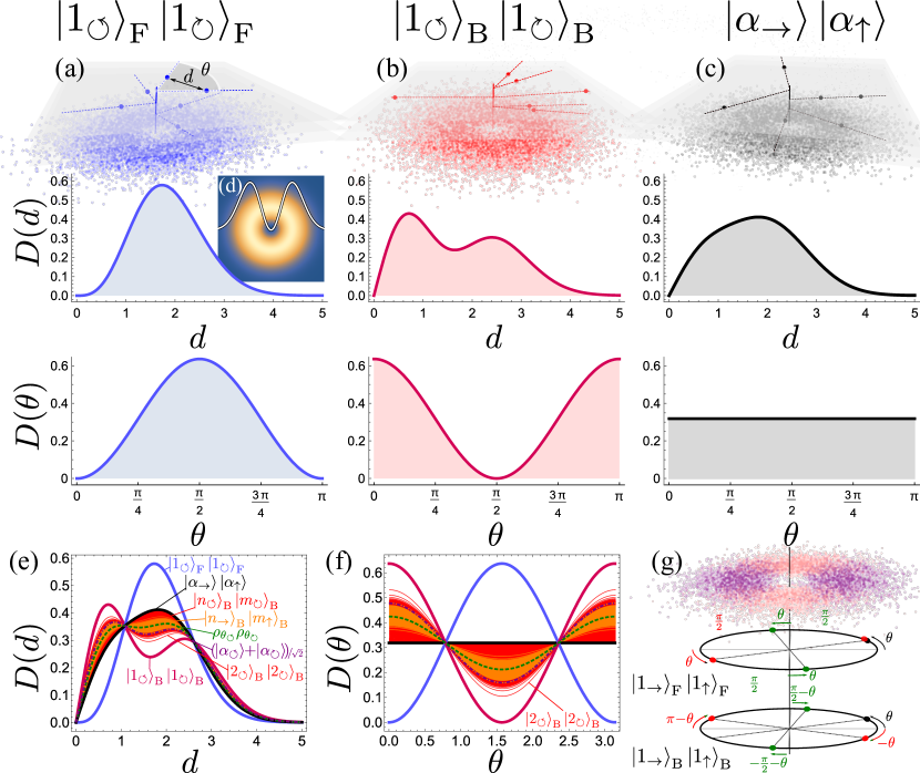
Figure 1: Top row: Single-shot realizations and their averages for Fock states $\ket{1_{\circlearrowleft}}\ket{1_{\circlearrowright}}$ with (a) Fermi F & (b) Bose B statistics, and (c) for coherent states. The sum over many realizations converge to the exact same vortex shape shown in (d). Second row: distributions $D(d)$ between any two particles from the corresponding column. Bosons present a bimodal distribution. Third row: distributions $D(\Delta\theta)$ of the angles between particles. (e–f) The three cases superimposed along with an enlarged family of quantum states, including unbalanced Fock states and thermal states. (g) Monte Carlo of distinguishable photons sampled from two dipoles, to reveal the underlying structure, and the angular correlations for fermions and bosons when these are indistinguishable in the donut. A particle at angle $\theta$ (black) suppresses red and stimulate green ones, resulting in rich spatial correlations.

Despite this mathematical identity of their one-photon reduced density matrix, all these states differ drastically for their two-photon reduced density matrix, as should be clear from Eqs. (4). A more “visible” and direct manifestation of such departures is shown in the figure, where we compare the three illustrative cases of (a & b) two Fock states with one particle in each vortex state and (c) two coherent states with mean amplitude one, so there is also one particle in each mode but this time on average and with poissonian fluctuations (thus also having no particle with the same probability $\approx 37\%$ than having one, and with more than one particle over one-fourth of the time). Although the density profiles for all cases, as reconstructed from averaging over the photons detected in isolation, are identical and recover the theoretical limit (shown in the Inset (d) both in 2D and with a cut along the radius), photons detected in pairs behave differently. The simplest quantity to measure is the distance between them. This is obtained from $\rho^{(2)}$ as $D(d)\equiv\langle{:}\hat{N}^{2}{:}\rangle^{-1}{\int\rho^{(2)}(\mathbf{r},\mathbf{r}^{\prime})\delta(\|\mathbf{r}-\mathbf{r}^{\prime}\|-d)\,\mathrm{d}\mathbf{r}\,\mathrm{d}\mathbf{r}^{\prime}}$ with $\langle{:}\hat{N}^{2}{:}\rangle=\int\rho^{(2)}(\mathbf{r},\mathbf{r}^{\prime})\,\mathrm{d}\mathbf{r}\,\mathrm{d}\mathbf{r}^{\prime}$ the normalization. The average is, this time, over (at least) two-photon observables. We show three such frames for each case at the top of the figure. Superimposing all these frames, one averages over the two-particle observables to recover the one-particle one as $\rho^{(1)}(\mathbf{r})=\int\rho^{(2)}(\mathbf{r},\mathbf{r}^{\prime})\,\mathrm{d}\mathbf{r}^{\prime}$. Experimentally, this corresponds to the acquisition of the density profile by integrating over the detected photons, washing out their correlations and properties in the process. Multiphoton correlations must thus be obtained from independent frames before their averaging, which constitutes a quantum measurement. The corresponding theoretical distributions for the three cases are shown below, with a singled-peak $D_{\mathrm{F}}(d)={1\over 2}d^{3}\exp(-d^{2}/2)$ for Fermions, a bimodal $D_{\mathrm{B}}(d)={1\over 8}(8-4d^{2}+d^{4})\exp(-d^{2}/2)$ for bosons and a flattened $D_{\mathrm{Coh}}(d)={1\over 16}d(8+d^{4})\exp(-d^{2}/2)$ for coherent states. Although bosons, with a mean separation of $\sqrt{121\pi/128}\approx 1.72$ time the vortex radius, are closer on average than fermions, whose mean separation is $\sqrt{9\pi/8}\approx 1.88$ (all distances are in units of the vortex radius), they present two local maxima, at both very small distances of $\approx 0.71$ and large ones $\approx 2.4$ as opposed to $\sqrt{3}\approx 1.73$ for fermions. In fact, bosonic Fock states are those most likely to distribute their two photons farther apart than a distance strictly greater than $d=2$. Curiously, all these quantum states have the same probability ($3/e^{2}$) to be found at a distance equal to the vortex diameter, and this remains true for the extended family considered in the Supplementary [35]. Also, all the distance distributions feature the same variance $\operatorname{Var}(d)=4$ despite corresponding to different quantum states. There are thus various peculiarities from even simple cases put in various quantum states. The bimodal curiosity is easily explained, as due to the spatial profile of the underlying state (the donut shape). If instead of the distances—which is easy to measure as this is absolute—we consider relative angles $\Delta\theta$ with respect to the donut center, then we can capture the essence of the phenomenon. This is shown in the third row, where we plot $D(\Delta\theta)\equiv{1\over\langle{:}\hat{N}^{2}{:}\rangle}\int\rho^{(2)}(\mathbf{r},\mathbf{r}^{\prime})\delta(\vartheta^{\prime}-\vartheta-\Delta\theta)\,\mathrm{d}\mathbf{r}\mathrm{d}\mathbf{r}^{\prime}$ for the respective cases. This results in the simpler $D_{\mathrm{F}}(\Delta\theta)={2\over\pi}\cos^{2}\Delta\theta$ and $D_{\mathrm{B}}(\Delta\theta)={2\over\pi}\sin^{2}\Delta\theta$ while $D_{\mathrm{Coh}}(\Delta\theta)=\mathrm{cste}$ ($1/\pi$ as normalization of the uniform distribution). This means that the geometric aspect which bosons and fermions extremize is not the distance, but the angle: fermions want to be perpendicular while bosons want to be aligned. The boson bimodal distribution is because if particles get aligned on the same side of the donut, they are close together, while if they are on the other side of the hole, they are farther apart than fermions, which are at right angle. Symmetrizing the angle alone is possible because vortices have a hole in their center, and fermions can never sit on each other as their only meeting point would be at the core, which has no particles. Aligned bosons can be found at the same position, but they do not maximize their spatial overlap by being on the same side of the donut. Their probability is still locally twice as much to be found at close distance $d\approx 0$ since $D_{\mathrm{B}}(d)\approx d$ while $D_{\mathrm{Coh}}(d)\approx d/2$ (compare with $D_{\mathrm{F}}(d)\approx d^{3}/2$) but this “spatial condensation” is because the perpendicular options are depleted (while the opposite one, maximizing distances, is also Bose stimulated). Coherent states wash out all traces of particle correlations, although bosonic symmetry is knitted in the fabric of the wavefunction, but this cancels out by disentangling, so that particles get distributed indiscriminately even in individual frames. The second row of the figure is thus best understood as the distribution for the law of cosines $D\equiv\sqrt{R_{1}^{2}+R_{2}^{2}-2R_{1}R_{2}\cos(\Theta)}$ for the independent random variables $R_{1}$ and $R_{2}$ sampling the radial profile $\rho_{1}(r)$ while $\Theta$ follows $D_{\mathrm{F}}$, $D_{\mathrm{B}}$ or $D_{\mathrm{Coh}}$, confirming that particles do not “care” about their distance per se, which is sampled randomly and independently, but about their angle, wherein lies the two-particle correlations. There are countless other quantum states that can correlate their photon pairs in a way which does not transpire through single-photon observables, and the most straightforward extensions to the Fock and coherent states are shown in Panels (e) for distances and (f) for angles, enclosed between the Bose and Fermi extrema of two particles. Cothermal states span continuously between the thermal and coherent boundaries and a precise measurement of this distribution would allow to extract information on the underlying quantum state, such as the coherent fraction of a Bose condensate. Vortices from two particles in the dipole basis are interesting in this respect. Fermions retain the same correlations in both bases, with the tendency, when a photon is detected at an angle $\theta$, to have the second one be detected at angles $\theta\pm{\pi\over 2}$ while suppressing those at $\theta+\pi$, as sketched in panel (g). This is clear from the quantum state expressed in both basis: $\ket{1_{\to},1_{\uparrow}}_{\mathrm{F}}=i\ket{1_{\circlearrowleft},1_{\circlearrowright}}_{\mathrm{F}}$. Bosonic dipoles, on the other hand, turn into NOON vortices $\ket{1_{\to},1_{\uparrow}}_{\mathrm{B}}={i\over\sqrt{2}}(\ket{2_{\circlearrowleft},0_{\circlearrowright}}-\ket{0_{\circlearrowleft},2_{\circlearrowright}})$ with, surprisingly, the distribution of distances of uncorrelated particles, i.e., $D_{\mathrm{coh}}(d)$. But this is not because they are, like coherent states, not correlated. On the opposite, they have even more complex correlations, requiring to keep track of two angles. We can indeed write the two-particle reduced density matrix for all cases in polar coordinates as

$$\rho^{(2)}(r,s,\theta,\vartheta)={2}r^{2}s^{2}e^{-r^{2}-s^{2}}D(\theta,\vartheta)/\pi^{2}\,,$$ (5)

where, in most cases, the two-angle distributions is rotation invariant and thus depend only on $\Delta\theta\equiv\theta-\vartheta$ as is the case for the distributions already given and plotted. Bosonic dipoles, on the other hand, have $D_{\ket{1_{\to},1_{\uparrow}}_{\mathrm{B}}}(\theta,\vartheta)={2\over\pi}\sin^{2}(\theta+\vartheta)$ with an absolute dependence of the angles (the rotation invariance is broken by the dipole orientation). This is sketched on the figure with a “first” detected photon (in black) at $\theta$ finding others more likely or suppressed, according to the bosonic stimulation of vortices at diagonal angles ($\theta=k\pi/4$ for integer $k$), but of fermionic ones at right angles ($k\pi/2$). This corresponds to antibunching of same-dipole arrangements and bunching of overlapping perpendicular dipoles. The averages of these competing cases result in uncorrelated distances, as if the resulting vortex was coherent, when it is, in fact, richly structured. Similarly, thermal states have the same correlations in either basis by averaging unbalanced Fock states $\ket{n,m}$ [35].

An exciting immediate follow-up of our approach is to query the bosonic character of excitonic vortices from such spatial correlations for two electron-hole pairs bound as excitons, so bosons, and thus expressing as a whole bunching tendencies, but with a built-in frustration of their constituents opposing Pauli repulsion [36]. Identifying which model, from simple phenomenological ones based on $q$-deformed algebra to exact full semiconductor Hamiltonians treatment, reproduces unequivocal experimental results, would resolve this thorny and longstanding controversy of solid-state physics [37, 38]. Then one can turn to a full dynamical (not stationary), interacting (not linear), multiphoton ($>2$) correlations in both space and time for arbitrary spatial profiles (not merely vortices). Two and three-photon vortex states have recently been created in strongly-interacting Rydberg gases [39], which also provide natural and even richer platforms for such characterizations. There is no end of problems to tackle in this way. Surprising correlations were noted early on from sub-atomic physics with unexpected bosonic effects even between distinguishable particles, due to intermediate-state and interference effects in multipion production [40]. Interestingly, this was linked to some innate capacity of the particles to produce squeezing. From our quantum-optical perspective, one can get direct control of the quantum states of the field to cover the full gamut of possibilities beyond the Bose-Einstein correlations found in stars and nucleis, and thus go at the bottom of these fascinating effects which started the modern theory of light.

Acknowledgments: This work was supported by the HORIZON EIC-2022-PATHFINDERCHALLENGES-01 HEISINGBERG project 101114978.

References

- [1] Brown, R. H. Boffin: A Personal Story of the Early Days of Radar, Radio Astronomy and Quantum Optics (CRC Press, 1991).
- [2] Hanbury Brown, R. & Twiss, R. Q. A test of a new type of stellar interferometer on Sirius. Nature 178, 1046 (1956). URL doi:10.1038/1781046a0.
- [3] Purcell, E. M. The question of correlation between photons in coherent light rays. Nature 178, 1449 (1956). URL doi:10.1038/1781449a0.
- [4] Baym, G. The physics of Hanbury Brown–Twiss intensity interferometry: from stars to nuclear collisions. Acta Physica Polonica B 29, 1839 (1998). URL http://th-www.if.uj.edu.pl/acta/vol29/abs/v29p1839.htm.
- [5] Weiner, R. M. Introduction to Bose-Einstein Correlations and Subatomic Interferometry (John Wiley and Sons, 2000).
- [6] Goldhaber, G., Goldhaber, S., Lee, W. & Pais, A. Influence of Bose–Einstein statistics on the antiproton-proton annihilation process. Phys. Rev. 120, 300 (1960). URL doi:10.1103/physrev.120.300.
- [7] Boal, D. H., Gelbke, C.-K. & Jennings, B. K. Intensity interferometry in subatomic physics. Rev. Mod. Phys. 62, 553 (1990). URL doi:10.1103/revmodphys.62.553.
- [8] ALICE collaboration. Two-pion Bose–Einstein correlations in central Pb–Pb collisions at TeV. Phys. Lett. B 696, 328 (2011). URL doi:10.1016/j.physletb.2010.12.053.
- [9] Natarajan, C. M., Tanner, M. G. & Hadfield, R. H. Superconducting nanowire single-photon detectors: physics and applications. Supercond. Sci. Technol. 25, 063001 (2012). URL doi:10.1088/0953-2048/25/6/063001.
- [10] Wang, Y. et al. Mid-infrared single-pixel imaging at the single-photon level. Nature Comm. 14, 1073 (2023). URL doi:10.1038/s41467-023-36815-3.
- [11] Lubin, G., Oron, D., Rossman, U., Tenne, R. & Yallapragada, V. J. Photon correlations in spectroscopy and microscopy. ACS Photonics 9, 2891 (2022). URL doi:10.1021/acsphotonics.2c00817.
- [12] Glauber, R. J. Photon correlations. Phys. Rev. Lett. 10, 84 (1963). URL doi:10.1103/PhysRevLett.10.84.
- [13] Kimble, H. J., Dagenais, M. & Mandel, L. Photon antibunching in resonance fluorescence. Phys. Rev. Lett. 39, 691 (1977). URL doi:10.1103/PhysRevLett.39.691.
- [14] Cohen-Tannoudji, C. & Reynaud, S. Atoms in strong light-fields: Photon antibunching in single atom fluorescence. Phil. Trans. R. Soc. Lond. A 293, 223 (1979). URL doi:10.1098/rsta.1979.0092.
- [15] Khalid, S. & Laussy, F. P. Perfect single-photon sources. Sci. Rep. 14, 2684 (2024). URL doi:10.1038/s41598-023-47585-9.
- [16] Dennis, M. R., O’Holleran, K. & Padgett, M. J. Singular optics: Optical vortices and polarization singularities. Progress in Optics 53, 293 (2009). URL doi:10.1016/S0079-6638(08)00205-9.
- [17] Shen, Y. et al. Optical vortices 30 years on: OAM manipulation from topological charge to multiple singularities. Light: Sci. & App. 8, 90 (2019). URL doi:10.1038/s41377-019-0194-2.
- [18] Rosen, G. F. Q., Tamborenea, P. I. & Kuhn, T. Interplay between optical vortices and condensed matter. Rev. Mod. Phys. 94, 035003 (2022). URL doi:10.1103/revmodphys.94.035003.
- [19] Kavokin, A., Baumberg, J. J., Malpuech, G. & Laussy, F. P. Microcavities (Oxford University Press, 2017), 2 edn.
- [20] Lagoudakis, K. G. et al. Quantized vortices in an exciton-polariton condensate. Nature Phys. 4, 706 (2008). URL doi:10.1038/nphys1051.
- [21] Fraser, M. D., Roumpos, G. & Yamamoto, Y. Vortex–antivortex pair dynamics in an exciton–polariton condensate. New J. Phys. 11, 113048 (2009). URL doi:10.1088/1367-2630/11/11/113048.
- [22] Sanvitto, D. et al. Persistent currents and quantized vortices in a polariton superfluid. Nature Phys. 6, 527 (2010). URL doi:10.1038/nphys1668.
- [23] Krizhanovskii, D. N. et al. Effect of interactions on vortices in a nonequilibrium polariton condensate. Phys. Rev. Lett. 104, 126402 (2010). URL doi:10.1103/PhysRevLett.104.126402.
- [24] Caputo, D. et al. Topological order and thermal equilibrium in polariton condensates. Nature Mater. 17 (2018). URL doi:10.1038/nmat5039.
- [25] Gnusov, I. et al. Quantum vortex formation in the “rotating bucket” experiment with polariton condensates. Science Advances 9, eadd1299 (2023). URL doi:10.1126/sciadv.add1299.
- [26] del Valle-Inclan Redondo, Y. et al. Optically driven rotation of exciton–polariton condensates. Nano Lett. 23, 4564 (2023). URL doi:10.1021/acs.nanolett.3c01021.
- [27] Dominici, L. et al. Coupled quantum vortex kinematics and berry curvature in real space. Commun. Phys. 6, 197 (2023). URL doi:10.1038/s42005-023-01305-x.
- [28] Panico, R. et al. Onset of vortex clustering and inverse energy cascade in dissipative quantum fluids. Nature Photon. 17, 451 (2023). URL doi:10.1038/s41566-023-01174-4.
- [29] Cuevas, A. et al. First observation of the quantized exciton-polariton field and effect of interactions on a single polariton. Science Advances 4, eaao6814 (2018). URL doi:10.1126/sciadv.aao6814.
- [30] Suárez-Forero, D. G. et al. Quantum hydrodynamics of a single particle. Light: Sci. & App. 9, 85 (2020). URL doi:10.1038/s41377-020-0324-x.
- [31] Boulier, T. et al. Polariton-generated intensity squeezing in semiconductor micropillars. Nature Comm. 5, 3260 (2014). URL doi:10.1038/ncomms4260.
- [32] Delteil, A. et al. Towards polariton blockade of confined exciton–polaritons. Nature Mater. 18, 219 (2019). URL doi:10.1038/s41563-019-0282-y.
- [33] Muñoz-Matutano, G. et al. Emergence of quantum correlations from interacting fibre-cavity polaritons. Nature Mater. 18, 213–218 (2019). URL doi:10.1038/s41563-019-0281-z.
- [34] Dominici, L. et al. Ultrafast control and Rabi oscillations of polaritons. Phys. Rev. Lett. 113, 226401 (2014). URL doi:10.1103/PhysRevLett.113.226401.
- [35] Supplementary material.
- [36] Laussy, F. P. & Kavokin, A. Excitons in crystals. Encycl. Cond. Mat. Phys. 3, 706 (2024). URL doi:10.1016/b978-0-323-90800-9.00163-3.
- [37] Laikhtman, B. Are excitons really bosons? J. Phys.: Condens. Matter 19, 295214 (2007). URL doi:10.1088/0953-8984/19/29/295214.
- [38] Combescot, M., Betbeder-Matibet, O. & Dubin, F. The many-body physics of composite bosons. Phys. Rep. 463, 215 (2008). URL doi:10.1016/j.physrep.2007.11.003.
- [39] Drori, L. et al. Quantum vortices of strongly interacting photons. Science 381, 193 (2023). URL doi:10.1126/science.adh5315.
- [40] Andreev, I. V., Plümer, M. & Weiner, R. M. Surprises from Bose–Einstein correlations. Phys. Rev. Lett. 67, 3475 (1991). URL doi:10.1103/physrevlett.67.3475.