Convergence of solutions of a one-phase Stefan problem with Neumann boundary data to a self-similar profile

Abstract

We study a one-dimensional one-phase Stefan problem with a Neumann boundary condition on the fixed part of the boundary. We construct the unique self-similar solution, and show that starting from arbitrary initial data, solution orbits converge to the self-similar solution.

Keywords: Stefan problem; Neumann boundary condition; large time behavior; self-similar profile.

2020 MSC: 35B40 35R35 35C06 80A22.

1 Introduction

1.1 On the content of the paper

The Stefan problem has been extensively studied in the past decades. Despite the number of articles and books published on this topic, [11], [8], [10], [9], there are still open problems left, see for instance [1], [3]. One of the questions which requires further attention is the long time behavior of the one-phase Stefan problem, where the heat flux is specified at the fixed boundary, namely the Neumann problem :

$$\begin{array}[]{cll}(i)&{u}_{t}(x,t)-u_{xx}(x,t)=0,&t>0,\ 0<x<s(t),\\ (ii)&-u_{x}(0,t)=\displaystyle{\frac{h}{\sqrt{t+1}}},\quad u(s(t),t)=0,&t>0,\\ (iii)&\dot{s}(t)=-u_{x}(s(t),t),&t>0,\\ (iv)&u(x,0)=u_{0}(x),&0<x<s(0)=b_{0},\end{array}$$ (1)

We stress that this type of boundary condition is reasonable from the modeling view point. Namely, the decay of data presented in (1-$ii$) is consistent with the parabolic scaling. We choose, however, to shift the initial time by a positive constant, say 1. In this way we avoid an artificial singularity at the initial time $t=0$. Let us note that the existence of a unique smooth solution $(u,s)$ to Problem (1) has already been established. We recall the assumptions of this result in Subsection 1.2. Here $u$ may be called the temperature and $s$ is the position of the interface.

Our approach to study the long time behavior of Problem (1) follows a general heuristics saying that the time asymptotics is determined by the steady states (there is none for (1)) or special solutions such as self-similar solutions or travelling waves. In fact, we show in Corollary 1 that there is exactly one self-similar solution $(v,\sigma)$, which has the form, $v(x,t)=U\left(\frac{x}{\sqrt{t+1}}\right)$ and $\sigma(t)=\omega\sqrt{t+1}$ for some constant $\omega$ and a profile function $U.$ Our main result states that the self-similar solution is attracting.

Theorem 1.

Suppose that $(u_{0},b_{0})$ satisfies the conditions

$$0\leq u_{0}\in W^{1,\infty}(0,+\infty),\quad 0<u_{0}(0)\ \text{ and }u_{0}(x)=0\,\text{in }[b_{0},\infty).$$ (2)

Let $(u,s)$ be the corresponding solution of Problem (1). Then,
 1) $\lim\limits_{t\to\infty}s(t)/\sqrt{t+1}=\omega$;
2) $\displaystyle{\lim\limits_{t\to\infty}\sup_{x/\sqrt{t+1}\in[0,\omega]}\left|u(x,t)-U\left(\frac{x}{\sqrt{t+1}}\right)\right|}=0.$

Our method of proof is based upon recent results obtained by [4], [3], who use the comparison principle in an essential way. The argument dwells on the possibility of trapping a given solution to (1) between two solutions with known time asymptotic behavior. In order to make this method work we transform (1) to a problem on a bounded domain with the help of similarity variables. The self-similar solution of (1) corresponds to the steady state solution of the transformed system. Its uniqueness is of crucial importance for the proof.

Let us stress the main difference between [4], [3] and the present article. The authors of [4] and [3] present a quite technical proof to show that the space derivative of the solution uniformly converges to its limit as $t\to\infty.$ Here, we completely avoid such a claim, so that our proof is simpler and more direct, which would make our method easier to adapt to a different setting.

We should point out that there are a number of results dealing with the asymptotic behavior of solutions of Stefan problems, mainly in the case of Dirichlet data on the fixed boundary. However, even for Dirichlet data, there are not so many articles besides [4] and [3] simultaneously addressing the behavior of the temperature profile $u$ and the shape of the interface $s.$

1.2 Existence and uniqueness of the solution

Let us stress that (2) is our standing set of assumptions on the initial conditions. Moreover, the condition $u_{0}(0)>0$ is necessary to construct proper lower solutions, but is not needed in the Proposition below:

Proposition 1.

Assume that the initial condition $u_{0}$ satisfies (2) and that $h>0$. Then, there exists a unique classical solution $(u,s)$ of Problem (1) for all $t>0$, in the following sense :

$$s\in{C^{1}}([0,\infty)),\quad u\in C^{2,1}(\{(x,t):t>0,0<x<s(t)\}),$$

$$u\in{C(\{(x,t):t\geq 0,0\leq x\leq s(t)\}}),u_{x}\in{C(\{(x,t):t>0,0\leq x\leq s(t)\})}.$$

We refer to [7, Chapter 8, Theorem 2] for the proof of this proposition.

Strictly speaking, the original statement in [7] required $u_{0}$ to be of class $C^{1}$; however, we may relax this assumption in view of [2, Theorem 5.1].

The organization of this paper is as follows. In Subsection 2.1 we discuss the existence and uniqueness of the self-similar solution. Subsection 2.2 is devoted to the study of upper and lower solutions as well as to estimates following from monotonicity. In the last Section, Section 3, we present the proof of the convergence result which is based on the comparison principle.

2 Self-similar, lower and upper solutions

2.1 Self-similar solution

We start by re-expressing Problem (1) in terms of the self-similar variables. In other words, we set

$$W(\eta,\tau)=u(x,t)\quad\hbox{and}\quad b(\tau)=\frac{s(t)}{\sqrt{t+1}},$$

where $\displaystyle{\eta=\frac{x}{\sqrt{t+1}}}$ and $\tau=\ln(t+1)$, to obtain the problem

$$\begin{array}[]{cll}(i)&W_{\tau}(\eta,\tau)-W_{\eta\eta}(\eta,\tau)-\displaystyle{\frac{\eta}{2}}W_{\eta}(\eta,\tau)=0&\tau>0,\ 0<\eta<b(\tau),\\ (ii)&-W_{\eta}(0,\tau)=h,\quad W(b(\tau),\tau)=0&\tau>0,\\ (iii)&\dot{b}(\tau)+\displaystyle{\frac{b(\tau)}{2}}=-W_{\eta}(b(\tau),\tau)&\tau>0,\\ (iv)&b(0)=b_{0}>0,\quad W(\eta,0)=u_{0}(\eta)&0<\eta<b_{0}.\end{array}$$ (3)

Let us remark that the existence and uniqueness of the stationary solution of problem (3) were given in [12].

Lemma 1.

The associated stationary problem to (3), which is given by

$$\begin{array}[]{ll}(i)&W_{\eta\eta}(\eta)+\displaystyle{\frac{\eta}{2}}W_{\eta}(\eta)=0,\quad 0<\eta<\omega,\\ (ii)&-W_{\eta}(0)=h,\quad W(\omega)=0,\\ (iii)&\displaystyle{\frac{\omega}{2}}=-W_{\eta}(\omega).\end{array}$$ (4)

admits a unique solution given by the pair $(U,\omega)$ such that

$$U(\eta)=h\displaystyle{\int_{\eta}^{\omega}e^{-\frac{s^{2}}{4}}\,ds},\qquad\eta\in[0,\omega]$$ (5)

and $\omega$ is the unique positive solution of the equation $h=\displaystyle{\frac{x}{2}e^{\frac{x^{2}}{4}}}.$

We immediately conclude from this result that

Corollary 1.

If we set $u(x,t)=U(\displaystyle{\frac{x}{\sqrt{t+1}}})$ and $\sigma=\omega\sqrt{t+1}$, then $(u,\sigma)$ is a solution to (1$-i$)–(1$-iii$).

2.2 Lower and upper solutions

Similarly as in [3] we define notions of lower and upper solutions of (3).

Definition 1.

We say that a pair of smooth functions $(\underline{W},\underline{b})$ (resp. $(\overline{W},\overline{b}))$ is a lower (resp. upper) solution of Problem (3) if

$$\begin{array}[]{cll}(i)&W_{\tau}(\eta,\tau)-W_{\eta\eta}(\eta,\tau)-\displaystyle{\frac{\eta}{2}}W_{\eta}(\eta,\tau)\leq 0\quad(\text{resp.}\geq 0),&\tau>0,\ 0<\eta<b(\tau),\\ (ii)&-W_{\eta}(0,\tau)\leq h\quad(\text{resp.}\geq h),&\tau>0,\\ (iii)&W(b(\tau),\tau)=0&\tau>0,\\ (iv)&\dot{b}(\tau)+\displaystyle{\frac{b(\tau)}{2}}\leq-W_{\eta}(b(\tau,\tau))\quad(\text{resp.}\geq-W_{\eta}(b(\tau,\tau)))&\tau>0,\\ (v)&b(0)\leq b_{0}\quad(\text{resp. }b(0)\geq b_{0})&\\ (vi)&W(\eta,0)\leq u_{0}(\eta)\quad(\text{resp. }W(\eta,0)\geq u_{0}(\eta))&0<\eta<b(0).\end{array}$$ (6)

The following comparison principle is a fundamental tool in our article.

Theorem 2.

Let $(\underline{W}_{1}(\eta,\tau),\underline{b}_{1}(\tau))$ (respectively, $(\overline{W}_{2}(\eta,\tau),\overline{b}_{2}(\tau))$) be the extensions by zero of the lower (respectively, upper solutions) of (3) corresponding to the data $(h_{1},{u_{0}}_{1},{b_{0}}_{1})$ (respectively, $(h_{2},{u_{0}}_{2},{b_{0}}_{2})$). If $h_{1}\leq h_{2}$, ${u_{0}}_{1}\leq{u_{0}}_{2}$ and ${b_{0}}_{1}\leq{b_{0}}_{2}$, then $\underline{b}_{1}(\tau)\leq\overline{b}_{2}(\tau)$ for every $\tau>0$ and $\underline{W}_{1}(\eta,\tau)\leq\overline{W}_{2}(\eta,\tau)$ for every $\eta\geq 0$ and $\tau\geq 0$.

Proof.

The proof is rather similar to those presented by [6, Lemma 2.2 and Remark 2.3] and [5, Lemma 3.5]. We omit it here. ∎

In fact, we will construct lower and upper solutions, which are independent of time. For this purpose, we present the perturbed stationary problem

$$\begin{array}[]{cll}(i)&W_{\eta\eta}(\eta)+\frac{1}{2}\lambda\eta W_{\eta}(\eta)=0&0<\eta<b_{\lambda},\\ (ii)&-W_{\eta}(0)=\tilde{h},&W(b_{\lambda})=0,\\ (iii)&\displaystyle{\frac{b_{\lambda}}{2}}=-W_{\eta}(b_{\lambda}).&\end{array}$$ (7)

whose solution is given by the pair $(U_{\lambda},b_{\lambda})$, where $U_{\lambda}(\eta)=\tilde{h}\int_{\eta}^{b_{\lambda}}e^{-\lambda s^{2}/4}{\rm d}s,$ for given $\lambda$, and $b_{\lambda}$ is the unique solution to

$$\tilde{h}=\frac{b_{\lambda}}{2}\,e^{\lambda b_{\lambda}^{2}/4}.$$ (8)

Remark 1.

It is easy to see that for every $\lambda>0$ and $\eta$ in $(0,b_{\lambda})$, $U_{\lambda}\geq 0$, $(U_{\lambda})_{\eta}<0$ and $(U_{\lambda})_{\eta\eta}>0$. In particular, $U_{\lambda}$ is a linear function for $\lambda=0$, and it is a strictly convex function if $\lambda>0$.

Lemma 2.

Let $(U_{\lambda},b_{\lambda})$ be a solution of (7). If $\tilde{h}\leq h$, then for all $\lambda>1$ $(U_{\lambda},b_{\lambda})$ is an independent of time lower solution to (3).

Proof.

First we show that if $\lambda>1$, solutions of (7) are lower solutions. Indeed

$$-\{({U_{\lambda}})_{\eta\eta}+\displaystyle{\frac{\eta}{2}}({U_{\lambda}})_{\eta}\}=-\{({U_{\lambda}})_{\eta\eta}+\lambda\displaystyle{\frac{\eta}{2}}({U_{\lambda}})_{\eta}\}-\displaystyle{\frac{\eta-\lambda\eta}{2}}({U_{\lambda}})_{\eta}=\displaystyle{\frac{\eta(\lambda-1)}{2}}({U_{\lambda}})_{\eta}<0,$$ (9)

for all $\eta\in(0,b_{\lambda})$. Now, from (8) and the inequality $e^{x}>x$ for all $x>0$, it holds that $0<b_{\lambda}=2\tilde{h}e^{\lambda b^{2}_{\lambda}/4}\leq\displaystyle{\frac{8\tilde{h}}{\lambda b^{2}_{\lambda}}}$, which implies that $b_{\lambda}\to 0$ as $\lambda\to\infty$; thus we can choose $\lambda$ large enough so that $b_{\lambda}<b_{0}$.

Next we show that we can choose $\lambda$ such that $U_{\lambda}\leq u_{0}$. On the one hand we have that

$$u_{0}(\eta)=u_{0}(0)+\int_{0}^{\eta}u_{0}^{\prime}(s)\,ds\geq u_{0}(0)-M\eta,\quad\text{for all }\,0\leq\eta\leq b_{0}.$$

On the other hand, for every $0<\eta<b_{\lambda}$, we deduce from the strict convexity of $U_{\lambda}$ discussed in Remark 1 that

$$U_{\lambda}(\eta)<U_{\lambda}(0)+\frac{U_{\lambda}(b_{\lambda})-U_{\lambda}(0)}{b_{\lambda}}\eta=U_{\lambda}(0)-\frac{U_{\lambda}(0)}{b_{\lambda}}\eta.$$ (10)

Also we remark that

$$U_{\lambda}(0)=\tilde{h}\int_{0}^{b_{\lambda}}e^{-\lambda s^{2}}{\rm d}s\leq\tilde{h}b_{\lambda}\to 0,\quad\lambda\to\infty,$$ (11)

and recall that by the hypothesis (2) $u_{0}(0)>0$. Thus, if we choose $\lambda$ large enough so that $b_{\lambda}<\displaystyle{\frac{u_{0}(0)}{M}}$ and $U_{\lambda}(0)<u_{0}(0),$ it follows that

$$U_{\lambda}(\eta)\leq u_{0}(\eta)\quad\hbox{for all }\eta\in[0,b_{\lambda}].$$ (12)

We conclude that $(U_{\lambda},b_{\lambda})$ is a lower solution according to Definition 1. ∎

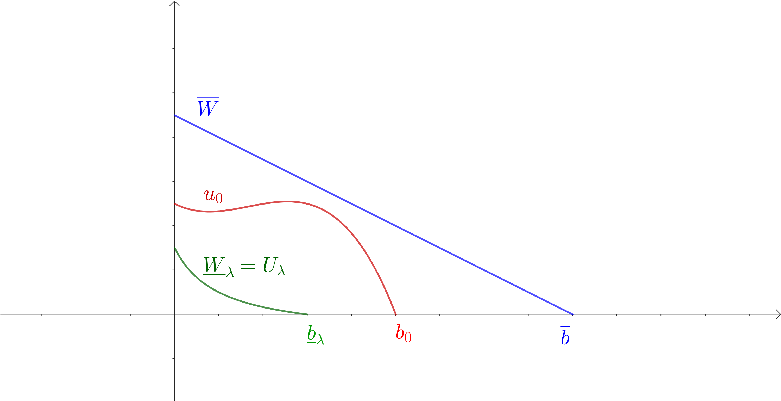
Figure 1: Lower and upper solutions

Now, we define the pair $(\underline{W}_{\lambda},\underline{b}_{\lambda})$ by

$$\underline{b}_{\lambda}=b_{\lambda}\quad\text{and}\quad\underline{W}_{\lambda}(\eta):=\begin{cases}U_{\lambda}(\eta)&\text{ if }0\leq\eta\leq\underline{b}_{\lambda},\\ 0&\text{ if }\eta>\underline{b}_{\lambda}\end{cases}.$$ (13)

Next we propose an upper solution which is a straight line on its support. It is easy to verify that the pair $(\overline{W},\overline{b})$ defined by

$$\overline{b}\geq b_{0}\,\text{ with }\,\overline{b}\geq 2h\quad\text{and}\quad\overline{W}(\eta):=\begin{cases}\displaystyle{\frac{\overline{b}}{2}}(\overline{b}-\eta),&\text{ if }0\leq\eta\leq\overline{b},\\ 0&\text{ if }\eta>\overline{b}\end{cases}$$ (14)

is an upper solution. Next, we give an additional condition in order to ensure that $U_{0}\geq u_{0}$ on the interval $[0,b_{0}]$. Since

$$u_{0}(\eta)\leq M(b_{0}-\eta)\mbox{ for all }\eta\in(0,b_{0}),$$

we deduce that if $\overline{b}\geq\sqrt{2Mb_{0}}$,

$$U_{0}(\eta)\geq u_{0}(\eta)\mbox{ for all }\eta\in(0,b_{0}),$$

which implies a similar property for $\overline{W}$.

3 Convergence

In this section, the pair $(\underline{W}_{\lambda},\underline{b}_{\lambda})$ is the lower solution for a fixed $\lambda$ given by (13) and $(\overline{W},\overline{b})$ is the upper solution given in (14). We shall write

$$\underline{W}(\eta,\tau):=W(\eta,\tau,(\underline{W}_{\lambda},\underline{b}_{\lambda})),\quad\underline{b}(\tau)=b(\tau,(\underline{W}_{\lambda},\underline{b}_{\lambda}))$$ (15)

and

$${\overline{W}}(\eta,\tau):=W(\eta,\tau,(\overline{W},\overline{b})),\quad\overline{b}(\tau)=b(\tau,(\overline{W},\overline{b}))$$ (16)

to denote solutions of (3).

Lemma 3.

Positivity and boundedness
There holds :

$$0\leq{\underline{W}}_{\lambda}(\eta)\leq{\underline{W}(\eta,\tau)}\leq W(\eta,\tau,u_{0},b_{0})\leq{\overline{W}(\eta,\tau)}\leq{\overline{W}}(\eta)\leq\displaystyle{\frac{\overline{b}^{2}}{2}},$$

and

$$0\leq b_{\lambda}\leq b(\tau,u_{0},b_{0})\leq\overline{b}.$$

Proof.

Repeatedly apply the comparison principle Theorem 2. ∎

Lemma 4.

[3] Monotonicity in time
a) The functions $\underline{W}(\eta,\tau)$ and $\underline{b}(\tau)$, are non-decreasing in time.
b) The functions ${\overline{W}}(\eta,\tau)$ and $\overline{b}(\tau)$, are non-increasing in time.

Proof.

We only prove part $a)$. For the sake of simplicity of notation we suppress the lower bar and we write $W$. From Theorem 2 we deduce that

$$W(\eta,s,(\underline{W}_{\lambda},\underline{b}_{\lambda}))\geq\underline{W}_{\lambda}(\eta)\quad\text{and }\quad b(s,(\underline{W}_{\lambda},\underline{b}_{\lambda}))\geq\underline{b}_{\lambda},\quad\text{for all }\,s\geq 0.$$ (17)

Now, for a fixed $s=\sigma$, we consider the pair $(W^{\sigma},b^{\sigma})$ where

$$W^{\sigma}(\eta)=W(\eta,\sigma,(\underline{W}_{\lambda},\underline{b}_{\lambda}))\quad\text{and }\quad b^{\sigma}=b(\sigma,(\underline{W}_{\lambda},\underline{b}_{\lambda})).$$ (18)

In particular we have $W^{\sigma}(\eta)\geq\underline{W}_{\lambda}(\eta)\quad\text{and }\quad b^{\sigma}\geq\underline{b}_{\lambda}.$ Then we apply again Theorem 2 to deduce that for every $\tau\geq 0$

$$W(\eta,\tau,(W^{\sigma},b^{\sigma})\geq W(\eta,\tau,(\underline{W}_{\lambda},\underline{b}_{\lambda}))\quad\text{and }\quad b(\tau,(W^{\sigma},b^{\sigma}))\geq b(\tau,(\underline{W}_{\lambda},\underline{b}_{\lambda})).$$ (19)

Returning to (17), now consider $s=\tau+\sigma$ for $\tau\geq 0$. It holds that the pair $(W(\eta,\tau+\sigma,(\underline{W}_{\lambda},\underline{b}_{\lambda})),b(\tau+\sigma,(\underline{W}_{\lambda},\underline{b}_{\lambda})))$ is a solution to problem (3) for the initial conditions (18) for every $\tau>0$. From the uniqueness of the solution we deduce that for all $\tau\geq 0$ we have

$$W(\eta,\tau,(W^{\sigma},b^{\sigma})=W(\eta,\tau+\sigma,(\underline{W}_{\lambda},\underline{b}_{\lambda}))\ \text{and }b(\tau,(W^{\sigma},b^{\sigma}))=b(\tau+\sigma,(\underline{W}_{\lambda},\underline{b}_{\lambda})).$$ (20)

Substituting (20) in (19) we deduce that

$$W(\eta,\tau+\sigma,(\underline{W}_{\lambda},\underline{b}_{\lambda}))\geq W(\eta,\tau,(\underline{W}_{\lambda},\underline{b}_{\lambda}))\text{ and }b(\tau+\sigma,(\underline{W}_{\lambda},\underline{b}_{\lambda}))\geq b(\tau,(\underline{W}_{\lambda},\underline{b}_{\lambda})),$$ (21)

which completes the proof of part a). ∎

We remark that if $(\underline{W},\underline{b})$ (resp. $({\overline{W}},\overline{b})$) is defined in (15) (resp. (16)), then the Lemmas 3 and 4 imply that for every $\lambda>0$

$$0<b_{\lambda}\leq\lim\limits_{\tau\rightarrow\infty}\underline{b}(\tau)=\underline{b}^{\infty}\leq\lim\limits_{\tau\rightarrow\infty}\overline{b}(\tau)=\overline{b}^{\infty}\leq\overline{b}.$$

In addition, the Lemmas 3 and 4 imply the convergence of $\underline{W}$ and ${\overline{W}}$, namely

$$0\leq\lim\limits_{\tau\rightarrow\infty}\underline{W}(\eta,\tau)=\underline{W}^{\infty}(\eta)\leq\frac{\overline{b}^{2}}{2},\ \mbox{for all }\,\eta\in[0,\underline{b}^{\infty}];\$$ (22)

and

$$0\leq\lim\limits_{\tau\rightarrow\infty}{\overline{W}}(\eta,\tau)={\overline{W}}^{\infty}(\eta)\leq\frac{\overline{b}^{2}}{2}\,\ \mbox{for all }\,\eta\in[0,\overline{b}^{\infty}).$$ (23)

Finally we state and prove the main result of this paper, which in turn implies the result of Theorem 1.

Theorem 3.

Let $(W(\eta,\tau,(u_{0},b_{0})),b(\tau,(u_{0},b_{0})))$ be the solution to the free boundary problem (3) associated to the initial data $(u_{0},b_{0})$. If $(W^{\infty},b^{\infty})$ is the unique steady state of (3) given by Lemma 1, then
(a) $\displaystyle{\lim_{\tau\to\infty}b(\tau)=b^{\infty}}$,
(b) $W(\cdot,\tau)$ converges to $W^{\infty}$ uniformly on $[0,\beta]$ for any $\beta\in(0,b^{\infty})$, when $\tau\to\infty$.
(c) At each time $\tau$ let us extend $W$ to $(0,\infty)^{2}$ by the formula

$$\tilde{W}(\eta,\tau)=\left\{\begin{array}[]{ll}W(\eta,\tau)&\eta\in[0,b(\tau)],\\ 0&\eta\in(b(\tau),\infty).\end{array}\right.$$

Then, $\tilde{W}(\cdot,\tau)$ converges uniformly to $\tilde{W}^{\infty}$, where

$$\tilde{W}^{\infty}(\eta)=\left\{\begin{array}[]{ll}W^{\infty}(\eta),&\eta\in[0,b^{\infty}],\\ 0,&\eta\in(b^{\infty},\infty).\end{array}\right.$$

Proof.

. Step 1. We have to identify the limits $\underline{W}_{\infty}$ and $\overline{W}^{\infty}$, and improve the convergence. For this purpose, we shall show the estimate,

$$\int_{T}^{T+1}\int_{0}^{b(\tau)}W_{\eta}^{2}(\eta,\tau)\,d\eta d\tau\leq M_{1},$$ (24)

where $W=\underline{W}$ or $W={\overline{W}}$ are the functions defined in (15) and (16), respectively.

In principle, we do not know if $W_{\eta\eta}$ and $W_{\tau}$ are square integrable over $\Omega_{T,1}:=\{(\eta,\tau):\eta\in(0,b(\tau)),\tau\in(T,T+1)\}$. This is why we set $\psi^{\delta}\in W^{1,\infty}(\{(\eta,\tau):\eta\in(0,b(\tau)),\tau\in(0,\infty)\})$

$$\psi^{\delta}(\eta,\tau)=\left\{\begin{array}[]{ll}0&\eta\in[0,\delta),\\ \frac{1}{\delta}(\eta-\delta)&\eta\in[\delta,2\delta),\\ 1&\eta\in[2\delta,b(\tau)-2\delta),\\ 1-\frac{1}{\delta}(\eta-b(\tau)+2\delta)&\eta\in[b(\tau)-2\delta,b(\tau)-\delta),\\ 0&\eta\in[b(\tau)-\delta,\infty)\end{array}\right.$$

and $\phi^{\delta}\in W^{1,\infty}((0,\infty))$, where

$$\phi^{\delta}(\tau)=\left\{\begin{array}[]{ll}0&\tau\in[0,T+\delta),\\ \frac{1}{\delta}(\tau-T-\delta)&\tau\in[T+\delta,T+2\delta),\\ 1&\tau\in[T+2\delta,T+1-2\delta)),\\ 1-\frac{1}{\delta}(\tau-(T+1-2\delta))&\tau\in[T+1-2\delta,T+1-\delta),\\ 0&\tau\in[T+1-\delta,\infty).\end{array}\right.$$

Finally, we set $\varphi^{\delta}(\eta,\tau)=\psi^{\delta}(\eta,\tau)\phi^{\delta}(\tau)$. Now, let us multiply the equation $(\ref{NSP-W})-(i)$ by $\varphi^{\delta}W$ and integrate over $\Omega_{T,1}$. We arrive at

$$L_{1}^{\delta}(T):=\int_{\Omega_{T,1}}WW_{\tau}\varphi^{\delta}\,d\eta d\tau=\int_{\Omega_{T,1}}(WW_{\eta\eta}+\frac{\eta}{2}W_{\eta}W)\varphi^{\delta}\,d\eta d\tau=:R_{1}^{\delta}(T).$$

We first analyze the left-hand-side, we see that integration by parts yields,

$$2L_{1}^{\delta}(T)=\int_{\Omega_{T,1}}\varphi^{\delta}(W^{2})_{\tau}\,d\tau d\eta=-\int_{\Omega_{T,1}}\varphi^{\delta}_{\tau}\ W^{2}\,d\tau d\eta.$$

The boundary terms vanish, because the support of $\varphi^{\delta}$ does not intersect $\partial\Omega_{T,1}.$ Now, we want to compute the limit $L_{1}(T)=\lim\limits_{\delta\to 0^{+}}L_{1}^{\delta}(T)$. We remark that

$$L_{1}(T)=\lim_{\delta\to 0^{+}}\left(-\frac{1}{2\delta}\int_{T}^{T+1}\int_{b(\tau)-2\delta}^{b(\tau)-\delta}\dot{b}(\tau)\phi^{\delta}(\tau)W^{2}(\eta,\tau)\,d\eta d\tau+\right.$$

$$\left.\frac{1}{2\delta}\int_{T+1-2\delta}^{T+1-\delta}\int_{0}^{b(\tau)}\psi^{\delta}W^{2}\,d\eta d\tau-\frac{1}{2\delta}\int_{T+\delta}^{T+2\delta}\int_{0}^{b(\tau)}\psi^{\delta}W^{2}\,d\eta d\tau\right).$$

For the limit in the first integral, note that from the continuity of the integrand, we can apply the mean value property for integrals to obtain that

$$\lim_{\delta\to 0^{+}}\frac{1}{2\delta}\int_{T}^{T+1}\int_{b(\tau)-2\delta}^{b(\tau)-\delta}\dot{b}(\tau)\phi^{\delta}(\tau)W^{2}(\eta,\tau)\,d\eta d\tau=\frac{1}{2}\int_{T}^{T+1}\dot{b}(\tau)W^{2}(b(\tau),\tau)\,d\tau.$$

Applying the condition at the moving boundary, we deduce that

$$\lim_{\delta\to 0^{+}}\frac{1}{2\delta}\int_{T}^{T+1}\int_{b(\tau)-2\delta}^{b(\tau)-\delta}\dot{b}(\tau)\phi^{\delta}(\tau)W^{2}(\eta,\tau)\,d\eta d\tau=0.$$

As for the other terms, we proceed in a similar way to deduce that

$$\lim_{\delta\to 0^{+}}\frac{1}{2\delta}\int_{T+1-2\delta}^{T+1-\delta}\int_{0}^{b(\tau)}\psi^{\delta}W^{2}\,d\eta d\tau=\frac{1}{2}\int_{0}^{b(T+1)}W^{2}(\eta,T+1)\,d\eta,$$

and that

$$\lim_{\delta\to 0^{+}}\frac{1}{2\delta}\int_{T+\delta}^{T+2\delta}\int_{0}^{b(\tau)}\psi^{\delta}W^{2}\,d\eta d\tau=\frac{1}{2}\int_{0}^{b(T)}W^{2}(\eta,T)\,d\eta,.$$

Hence, we conclude that

$$L_{1}(T)=\frac{1}{2}\int_{0}^{b(T+1)}W^{2}(\eta,T+1)\,d\eta-\frac{1}{2}\int_{0}^{b(T)}W^{2}(\eta,T)\,d\eta.$$

Next we consider the term $R^{\delta}_{1}(T)$. We integrate by parts to obtain

$$R^{\delta}_{1}(T)=-\int_{\Omega_{T,1}}(W_{\eta}^{2}\varphi^{\delta}+WW_{\eta}\varphi^{\delta}_{\eta}+\frac{1}{4}W^{2}(\eta\varphi^{\delta}_{\eta}+\varphi^{\delta}))\,d\eta d\tau.$$

Again here, the boundary terms vanish, because the support of $\varphi^{\delta}$ is contained in $\Omega_{T,1}$. We remark that the same argument as above leads us to

$$\lim_{\delta\to 0^{+}}\int_{\Omega_{T,1}}WW_{\eta}\varphi^{\delta}_{\eta}\,d\eta d\tau =\lim_{\delta\to 0^{+}}\frac{1}{\delta}\int_{T}^{T+1}\left(\int_{\delta}^{2\delta}WW_{\eta}\phi^{\delta}\,d\eta d\tau-\int_{b(\tau)-2\delta}^{b(\tau)-\delta}WW_{\eta}\phi^{\delta}\,d\eta d\tau\right)$$

$$=\int_{T}^{T+1}(-hW(0,\tau)-W(b(\tau),\tau)W_{\eta}(b(\tau),\tau))\,d\eta d\tau$$

$$=-\int_{T}^{T+1}hW(0,\tau)\,d\eta d\tau,$$

where we have also used the boundary condition (3$-ii$) as well as the condition at the interface (3$-iii$). Similarly one can show that

$$\lim_{\delta\to 0^{+}}\int_{\Omega_{T,1}}\frac{1}{4}W^{2}(\eta\varphi^{\delta}_{\eta}+\varphi^{\delta}))\,d\eta d\tau=\frac{1}{4}\int_{\Omega_{T,1}}W^{2}(\eta,\tau)\,d\eta d\tau.$$

Hence, we conclude

$$R_{1}(T)=\lim_{\delta\to 0^{+}}R^{\delta}_{1}(T)=-\int_{\Omega_{T,1}}W_{\eta}^{2}\,d\tau d\eta+h\int_{T}^{T+1}W(0,\tau)\,d\tau-\frac{1}{4}\int_{\Omega_{T,1}}W^{2}\,d\tau d\eta.$$

In view of Lemma 3 a possible choice of the constant $M_{1}$ is given by

$$M_{1}=h\frac{\overline{b}^{2}}{2}+\frac{\overline{b}^{5}}{8}.$$

Step 2. Applying the mean value theorem for integrals in (24) we deduce from Step 1 that there exist two sequences of points $\tau_{n}^{\prime},\tau_{n}^{\prime\prime}\in[n,n+1)$ such that

$$\int_{0}^{{\underline{b}}(\tau_{n}^{\prime})}\underline{W}_{\eta}^{2}(\eta,\tau_{n}^{\prime})\,d\eta,\quad\int_{0}^{{\overline{b}}(\tau_{n}^{\prime\prime})}\overline{W}_{\eta}^{2}(\eta,\tau_{n}^{\prime\prime})\,d\eta\leq M_{1}.$$ (25)

Since $\underline{b}(\tau_{n}^{\prime})\leq{\underline{b}}^{\infty}\leq{\overline{b}}^{\infty}\leq\overline{b}(\tau_{n}^{\prime\prime})$, it follows that (25) implies the bounds

$$\|\underline{W}_{\eta}(\cdot,\tau_{n}^{\prime})\|_{L^{2}(0,\beta)},\ \|\overline{W}_{\eta}(\cdot,\tau_{n}^{\prime\prime})\|_{L^{2}(0,{\overline{b}}^{\infty})}\leq\sqrt{M_{1}}$$ (26)

for all $\beta\in(0,{\underline{b}}^{\infty})$. Hence, we can select subsequences (not relabelled) such that

$$\underline{W}_{\eta}(\cdot,\tau_{n}^{\prime})\rightharpoonup\psi^{\beta}\hbox{ in }L^{2}(0,\beta)\quad\hbox{and}\quad\overline{W}_{\eta}(\cdot,\tau_{n}^{\prime\prime})\rightharpoonup\Psi\hbox{ in }L^{2}(0,\overline{b}^{\infty}).$$

Since the limit is unique, we deduce that $\psi^{\beta}$ and $\Psi$ do not depend on the choice of the sequence $\tau_{n}$ and using (22) and (23) we conclude that $\psi^{\beta}$ is the weak derivative of $\underline{W}_{\eta}^{\infty}$ in every interval $(0,\beta)$ and that $\Psi=\overline{W}_{\eta}^{\infty}$. So that $\underline{W}^{\infty}{\chi_{(0,\beta)}}\in H^{1}(0,\beta)$ for all $\beta\in(0,{\underline{b}}^{\infty})$ and thus $\overline{W}^{\infty}\in H^{1}(0,\overline{b}^{\infty})$. In fact, $\underline{W}^{\infty}\in H^{1}(0,{\underline{b}}^{\infty})$. Indeed, in view of Lebesgue monotone convergence theorem we have

$$\lim_{\beta\rightarrow{\underline{b}}^{\infty}}\int_{0}^{\underline{b}^{\infty}}({\underline{W}}_{\eta}^{\infty})^{2}(\eta)\chi_{(0,\beta)}(\eta)\,d\eta=\int_{0}^{{\underline{b}}^{\infty}}({\underline{W}}_{\eta}^{\infty})^{2}(\eta)\,d\eta\leq M_{1}.$$

Step 3. We claim that $(\underline{W}^{\infty},{\underline{b}}^{\infty})$ and $(\overline{W}^{\infty},{\overline{b}}^{\infty})$ are both stationary solutions, namely solutions of (4). Hence they are smooth and equal. Indeed, we multiply the equation (3-$i$) by $\varphi\in C^{\infty}_{c}(\mathbb{R})$ such that $\varphi_{\eta}(0)=0$ and we integrate on $\Omega_{T,1}$. Proceeding as in step 2 we set

$$L_{2}(T)=\int_{\Omega_{T,1}}W_{\tau}\varphi\,d\eta d\tau=\int_{\Omega_{T,1}}(W_{\eta\eta}\varphi+\frac{\eta}{2}W_{\eta}\varphi)\,d\eta d\tau=R_{2}(T).$$

$$L_{2}(T) =\int_{\Omega_{T,1}}W_{\tau}(\eta,\tau)\varphi(\eta)\,d\eta d\tau$$

$$=\int_{0}^{b(T+1)}W(\eta,T+1)\varphi(\eta)\,d\eta-\int_{0}^{b(T)}W(\eta,T)\varphi(\eta)\,d\eta,$$

where $W=\underline{W}$ or $W=\overline{W}$. We then deduce from Lebesgue’s dominated convergence theorem that $\lim_{T\to\infty}L_{2}(T)=0.$

Next, we investigate the right-hand-side $R_{2}(T)$. Integration by parts yields

$$R_{2}(T) =\int_{\Omega_{T,1}}W_{\eta\eta}\varphi\,d\eta d\tau+\int_{\Omega_{T,1}}\frac{\eta}{2}W_{\eta}\varphi\,d\eta d\tau$$

$$=\int_{\Omega_{T,1}}W(\varphi_{\eta\eta}-\frac{1}{2}(\eta\varphi)_{\eta})\,d\eta d\tau-\int_{T}^{T+1}(\dot{b}+\frac{b}{2})\varphi(b(\tau))+h\varphi(0).$$

Now, we pass to the limit as $T\rightarrow\infty$. It follows from Lebesgue’s dominated convergence theorem that

$$\lim_{T\to\infty}\int_{\Omega_{T,1}}W(\eta,\tau)(\varphi_{\eta\eta}-\frac{1}{2}(\eta\varphi)_{\eta})\,d\eta d\tau=\int_{0}^{b^{\infty}}W^{\infty}(\eta)(\varphi_{\eta\eta}-\frac{1}{2}(\eta\varphi)_{\eta})\,d\eta,$$

where $(W^{\infty},b^{\infty})$ is either $(\underline{W}^{\infty},{\underline{b}}^{\infty})$ or $(\overline{W}^{\infty},{\overline{b}}^{\infty})$. Let us denote by $\Phi$ an antiderivative of $\varphi$. Then,

$$\lim_{T\to\infty}\int_{T}^{T+1}\dot{b}\varphi(b(\tau))\,d\tau=\lim_{T\to\infty}(\Phi(b(T+1))-\Phi(b(T)))=0.$$

In addition,

$$\lim_{T\to\infty}\int_{T}^{T+1}\frac{b}{2}\varphi(b(\tau))\,d\tau=\frac{1}{2}b^{\infty}\varphi(b^{\infty}).$$

Finally, we collect all the results concerning $R_{2}(T)$, while keeping in mind that $\lim_{T\to\infty}L_{2}(T)=0$. This yields

$$0=\lim_{T\to\infty}R_{2}(T)=\int_{0}^{b^{\infty}}W^{\infty}(\eta)(\varphi_{\eta\eta}-\frac{1}{2}(\eta\varphi)_{\eta})\,d\eta-\frac{b^{\infty}}{2}\varphi(b^{\infty})+h\varphi(0),$$ (27)

for all smooth functions $\varphi$ in $\mathbb{R}$ such that $\varphi_{\eta}(0)=0$. In particular $W^{\infty}$ satisfies the differential equation (4-$i$) in the sense of distributions.

Step 4. We recall that $W^{\infty}\in H^{1}(0,b^{\infty})$. It is easy to infer from (27) that $W^{\infty}_{\eta\eta}=-\displaystyle{\frac{\eta}{2}}W^{\infty}_{\eta}\in L^{2}(0,b^{\infty})$, which in turn implies that $W^{\infty}\in H^{2}(0,b^{\infty})$.

Next we search for the boundary condition and the conditions on the moving boundary satisfied by $W^{\infty}$. After integrating by parts twice in (27) we obtain,

$$0 =\int_{0}^{b^{\infty}}(W^{\infty}_{\eta\eta}+\frac{\eta}{2}W^{\infty}_{\eta})\varphi\,d\eta+W^{\infty}\varphi_{\eta}|_{\eta=0}^{\eta=b^{\infty}}-W^{\infty}_{\eta}\varphi|_{\eta=0}^{\eta=b^{\infty}}$$

$$-\frac{b^{\infty}}{2}\varphi(b^{\infty})(W^{\infty}(b^{\infty})+1)+h\varphi(0),$$

so that

$$0= W^{\infty}(b^{\infty})\varphi_{\eta}(b^{\infty})-W^{\infty}_{\eta}(b^{\infty})\varphi(b^{\infty})+W^{\infty}_{\eta}(0)\varphi(0)$$

$$-{\frac{b^{\infty}}{2}}\varphi(b^{\infty})(W^{\infty}(b^{\infty})+1)+h\varphi(0),$$ (28)

for all smooth functions $\varphi$ on $\mathbb{R}$ such that $\varphi_{\eta}(0)=0$. Now, if we additionally choose $\varphi$ such that $\varphi(b^{\infty})=\varphi_{\eta}(b^{\infty})=0$, then (3) reduces to

$$\varphi(0)(W^{\infty}_{\eta}(0)+h)=0,$$

and since $\varphi(0)$ is arbitrary, we deduce that

$$W^{\infty}_{\eta}(0)+h=0.$$

Thus (3) becomes

$$0=W^{\infty}(b^{\infty})\varphi_{\eta}(b^{\infty})-W^{\infty}_{\eta}(b^{\infty})\varphi(b^{\infty})-{\frac{b^{\infty}}{2}}\varphi(b^{\infty})(W^{\infty}(b^{\infty})+1).$$ (29)

Next we suppose that $\varphi(b^{\infty})=0$, but $\varphi_{\eta}(b^{\infty})\neq 0$. Then

$$W^{\infty}(b^{\infty})\varphi_{\eta}(b^{\infty})=0,$$

and hence

$$W^{\infty}(b^{\infty})=0.$$

Then, (29) becomes

$$0=-W^{\infty}_{\eta}(b^{\infty})\varphi(b^{\infty})-{\frac{b^{\infty}}{2}}\varphi(b^{\infty}).$$ (30)

Suppose that $\varphi(b^{\infty})\neq 0$. Then (30) implies that

$$W^{\infty}_{\eta}(b^{\infty})=-\frac{b^{\infty}}{2}.$$

We deduce that the solution pair $(W^{\infty},b^{\infty})$ coincides with the unique solution of Problem (4) or in other words with the unique steady state solution of the time evolution problem, Problem (3).

Step 5. We recall that, in view of step 4, $W^{\infty}\in H^{2}(0,b^{\infty})\subset C^{1,\frac{1}{2}}([0,b^{\infty}])$. Moreover, the convergence of $\overline{W}$ to $W^{\infty}$ (resp. ${\tilde{\underline{W}}}$ to $W^{\infty}$) is monotone on $[0,b^{\infty}]$. Hence, we deduce with the help of Dini’s Theorem that this convergence is uniform.

Finally, since $b_{\lambda}\leq b_{0}\leq\overline{b}$ and since ${\underline{w}}_{\lambda}\leq u_{0}\leq{\overline{W}}$, the comparison principle implies that ${\underline{b}}(\tau)\leq b(\tau)\leq{\overline{b}}(\tau)$ and ${\tilde{\underline{W}}(\eta,\tau)\leq\tilde{W}(\eta,\tau)}\leq W(\eta,\tau)\leq\overline{W}(\eta,\tau)$ for all $(\eta,\tau)$. We conclude that $b(\tau)\rightarrow b^{\infty}$ and that $\tilde{W}(\tau)$ converges to $W^{\infty}$ uniformly on compact sets of $[0,\infty)$ as $\tau\rightarrow\infty$. ∎

Now, Theorem 1 easily follows from Theorem 3.

Acknowledgments

The second author, SR, was partly supported by the Project INV-006-00030 from Universidad Austral and PICT-2021-I-INVI-00317. The work of the second author, PR, was in part supported by the National Science Centre, Poland, through the grant number 2017/26/M/ST1/00700. A part of the work was performed while DH and SR visited the University of Warsaw, whose hospitality is greatly appreciated.

References

- [1] T. Aiki, A. Muntean, A free-boundary problem for concrete carbonation: Front nucleation and rigorous justification of the -law of propagation, Interfaces Free Bound., 15 (2012), 167-180.
- [2] D. Andreucci, Lecture Notes on the Stefan Problem, Universita di Roma La Sapienza (2004).
- [3] M. Bouguezzi, D. Hilhorst, Y. Miyamoto and J. F. Scheid, Convergence to a self-similar solution for a one-phase Stefan problem arising in corrosion theory, European J. Appl. Math. 34 (2023), 701–737.
- [4] M. Bouguezzi, Modeling and computer simulation of the propagation rate of pit corrosion, Ph.D thesis Université Paris-Saclay (2021).
- [5] Y. Du and Z. Lin, Spreading-vanishing dichotomy in the diffusive logistic model with a free boundary, SIAM J. Math. Anal., 42 (2010), 377–405.
- [6] Y. Du and B. Lou, Spreading and vanishing in nonlinear diffusion problems with free boundaries, J. Eur. Math. Soc. 17 (2015), 2673–2724.
- [7] A. Friedman, Partial Differential Equations of Parabolic Type, (Prentice-Hall, 1964).
- [8] A. Friedman, Variational Principles and Free Boundary Broblems, (Robert E. Krieger Publishing Co. Inc.,1988).
- [9] S. C. Gupta, The Classical Stefan Problem. Basic Concepts, Modelling and Analysis, (Elsevier, 2018).
- [10] A. Meirmanov, The Stefan Problem, (Walter de Gruyter, 1992).
- [11] L.I. Rubinstein, The Stefan Problem, Translations of Mathematical Monographs 27, (American Mathematical Society, 1971).
- [12] Tarzia, D. A., An inequality for the coeficient of the free boundary of the Neumann solution for the two-phase Stefan problem, Quart. Appl. Math. 39 (1981), 491–497.