Solving coupled Non-linear Schrödinger Equations via Quantum Imaginary Time Evolution

Abstract

Coupled non-linear Schrödinger equations are crucial in describing dynamics of many particle systems. We present a quantum imaginary time evolution (ITE) algorithm as a solution to such equations in the case of nuclear Hartree-Fock equations. Under a simplified Skyrme interaction model, we calculate the ground state energy of an oxygen-16 nucleus and demonstrate that the result is in agreement with the classical ITE algorithm.

I Introduction

The dynamics of quantum systems are described by the Schödinger equation. For many particle systems the potential is often dependent on the particle configuration itself. In such case the Schrödinger equation governing the system is a non-linear differential equation. When the particles in question are of different types, they are each described by separate equations, with a potential they all contribute in. The non-linear differential equations are then coupled to each other. Finding the solution to such equations, however, has proven to be computationally challenging. The dimension of the Hilbert space increases exponentially with the number of particles/states within the system and quickly exceeds current computing capacity with even the simplest system.

Quantum computers, on the other hand, are believed to be able to handle such calculations by handling information more efficiently and exploiting quantum entangling. One major advantage of quantum computers over classical computers is to simulate other quantum systems [1]. For instance, wave functions of many particle systems can be more efficiently encoded by qubits than by bits. This idea has been widely used in fields like quantum chemistry [2, 3, 4, 5], materials [6, 7], and nuclear physics [8, 9, 10, 11].

We previously presented an approach to solving the nuclear Hartree-Fock equation for ^4He via quantum imaginary time evolution (ITE) [12], which involves finding the solution of a non-linear Schrödinger equation. In this paper we give an expansion of the previous algorithm to include coupled non-linear Schrödinger equations. Using the ^16O nucleus as an example, we show that our implementation gives identical results as the classical ITE algorithm, while demonstrating a method for solving a set of coupled non-linear differential equations.

II Imaginary Time Evolution

The time evolution of a state $\ket{\psi\left(\vec{r},t\right)}$ under the Hamiltonian $\hat{H}$ is described by the time-dependent Schrödinger equation (TDSE)

$$\hat{H}\ket{\psi\left(\vec{r},t\right)}=i\hbar\frac{\partial}{\partial t}\ket{\psi\left(\vec{r},t\right)}\text{,}$$ (1)

which can be re-written in imaginary time ($t\rightarrow i\tau$) as

$$\frac{\partial}{\partial\tau}\ket{\psi\left(\vec{r},\tau\right)}=\frac{\hat{H}}{\hbar}\ket{\psi\left(\vec{r},\tau\right)}\text{.}$$ (2)

Given an initial state $\ket{\psi\left(\vec{r},0\right)}$, the time evolution gives the general solution of $\ket{\psi\left(\vec{r},\tau\right)}$ by

$$\ket{\psi\left(\vec{r},\tau\right)}=\mathcal{N}\exp(-\int_{0}^{\tau}\frac{\hat{H}}{\hbar}d\tau^{\prime})\ket{\psi\left(\vec{r},0\right)}\text{,}$$ (3)

where $\mathcal{N}$ is a normalization operator to renormalize the state after the application of the non-unitary imaginary time evolution operator. When $\tau\rightarrow\infty$, $\ket{\psi\left(\vec{r},\tau\right)}$ converges to the ground state of $\hat{H}$, provided that the initial state $\ket{\psi\left(\vec{r},0\right)}$ is not orthogonal to it [12, 13].

For a time-dependent Hamiltonian $\hat{H}(\tau^{\prime})$, the integral in equation (3) can be approximated by

$$-\int_{0}^{\tau}\frac{\hat{H}(\tau^{\prime})}{\hbar}d\tau^{\prime}\approx-\frac{\Delta\tau}{\hbar}\sum_{k=0}^{k_{total}}\hat{H}(k\Delta\tau)\text{,}$$ (4)

where $\Delta\tau=\frac{\tau}{k_{total}}$ is the imaginary time step and $k_{total}$ is the total number of steps. Although the Hamiltonian we use is independent of real time, we adopt an iterative approach and treat its non-linearity as an imaginary time dependence [13]. Using first order Suzuki-Trotter decomposition [14]

$$e^{\delta(A+B)}=e^{\delta A}e^{\delta B}+O(\delta^{2})\text{,}$$ (5)

equation (3) can be rewritten as

$$\ket{\psi\left(\vec{r},\tau\right)}=\prod_{k=0}^{k_{total}}\hat{U}_{k}\left(\Delta\tau\right)\ket{\psi\left(\vec{r},0\right)}\text{,}$$ (6)

where the ITE operator $\hat{U}_{k}$ is given by

$$\hat{U}_{k}\left(\Delta\tau\right)=\mathcal{N}\exp[-\frac{\Delta\tau}{\hbar}\hat{H}(k\Delta\tau)]\text{.}$$ (7)

With a sufficiently small imaginary time step $\Delta\tau\ll 1$, $\hat{U}_{k}$ can be approximated by

$$\hat{U}_{k}(\Delta\tau)\approx\mathcal{N}\left[1-\frac{\Delta\tau}{\hbar}\hat{H}(k\Delta\tau)\right]\text{.}$$ (8)

III ^16O Nuclear Model

In our previous work we used ^4He under a simplified Skyrme force [12, 15, 16, 17] as our test model. In this work we will assume the same simplified effective interaction with the radial Hatree-Fock Hamiltonian

$$\hat{H}_{\mathrm{hf}}^{l} =-\frac{\hbar^{2}}{2m}\left[\frac{d^{2}}{dr^{2}}-\frac{l\left(l+1\right)}{r^{2}}\right]$$ (9)

$$\quad+\left[\frac{3}{4}t_{0}\rho\left(r\right)+\frac{3}{16}t_{3}\rho^{2}\left(r\right)\right]\text{,}$$

where $t_{0}$ and $t_{3}$ are Skyrme force parameters. The density is given by

$$\rho\left(r\right)=\frac{1}{\pi r^{2}}\sum_{n,l}\left(2l+1\right)\left|u_{nl}\right|^{2}\text{,}$$ (10)

where $u_{nl}/{r}$ are the radial component of the single particle (SP) wave functions $\varphi_{nlmm_{s}q}\left(\vec{r},s,I_{3}\right)$. Spin and isospin degeneracies are accounted for with a factor of 4.

In ^4He all four nucleons are in the $0s_{1/2}$ state ($l=0$), and there is only one non-linear Schrödinger like equation to solve. In the ^16O case, the $0s_{1/2}$ ($l=0$), $0p_{1/2}$ ($l=1$, $m=0$), and $0p_{3/2}$ ($l=1$, $m=\pm 1$) states are all fully occupied. Since the $0p_{1/2}$ and $0p_{3/2}$ states share the same radial spatial wave function, this corresponds to two coupled non-linear Schrödinger like equations. The Hamiltonians for the $s$ states and $p$ states differ in the kinetic term,

$$T^{0} =-\frac{\hbar^{2}}{2m}\frac{d^{2}}{dr^{2}}$$ (11)

$$T^{1} =-\frac{\hbar^{2}}{2m}\left(\frac{d^{2}}{dr^{2}}-\frac{2}{r^{2}}\right)\text{,}$$

and share the same potential term

$$V^{0}=V^{1}=V(r)=\frac{3}{4}t_{0}\rho\left(r\right)+\frac{3}{16}t_{3}\rho^{2}\left(r\right)\text{,}$$ (12)

where

$$\rho\left(r\right)=\frac{1}{\pi r^{2}}\left(\left|u_{00}\right|^{2}+3\left|u_{01}\right|^{2}\right)\text{.}$$ (13)

Hence we have the radial Hatree-Fock equations for $s$ states,

$$\left[-\frac{\hbar^{2}}{2m}\frac{d^{2}}{dr^{2}}+V(r)\right]u_{00}=\varepsilon_{00}u_{00}\text{,}$$ (14)

and $p$ states,

$$\left[-\frac{\hbar^{2}}{2m}\frac{d^{2}}{dr^{2}}+\frac{\hbar^{2}}{mr^{2}}+V(r)\right]u_{01}=\varepsilon_{01}u_{01}\text{,}$$ (15)

where $\varepsilon_{0l}$ are SP energies for the corresponding states.

These two equations are coupled explicitly through the appearance of both $u_{00}$ and $u_{01}$ in the potential $V(r)$.

IV Quantum Implementation

We encode our states in the 3D isotropic oscillator basis (with oscillator length $\frac{1}{b}$ and corresponding angular momentum $l$) [18, 19, 20, 17]

$$u_{nl}\left(r\right)=\sum_{n^{\prime}}\alpha_{nln^{\prime}}\mathcal{R}^{b,l+\frac{3}{2}}_{n^{\prime}}\left(r\right),\;\;\alpha_{nln^{\prime}}\in\mathbb{R}\>\forall\>n,l,n^{\prime}\text{,}$$ (16)

where the $2^{N}$ expansion coefficients $\alpha_{nln^{\prime}}$ are stored in $N$ target qubits. Matrix elements of the density in the basis are then computed as a sum of of integrals of the product of four oscillator radial wave functions $\mathcal{R}^{b,l+\frac{3}{2}}_{n^{\prime}}\left(r\right)$, [12]

$$\rho^{l}\sim\sum_{j}\int\frac{dr}{r^{2}}\mathcal{R}^{l}\mathcal{R}^{l}\mathcal{R}^{j}\mathcal{R}^{j}\text{,}$$ (17)

where $\rho^{l}$ indicates the sub-basis $\rho(r)$ is expanded in. These calculated integrals are tabulated at the beginning and used in each step of ITE.

Once the matrix form of the pre-normalised ITE operator $\hat{U}_{k}$ is obtained, it is decomposed into a sum of products of Pauli matrices (and identity matrices) acting on individual qubits [21]. This non-unitary Hermitian gate is implemented using the idea of a duality computer [22, 23], with the aid of $2N$ auxiliary qubits and following the approach outlined in our previous work [12].

Figure 1: Quantum circuit for an ITE step in $N=1$ case. The state preparation subcircuits $SP(\mathfrak{N})$ are given in Appendix A.

V Results

We applied the approach above, using a classical algorithm and on a quantum simulator separately, to calculate the ground state energy of ^16O [24], for $N=1$ (2 expansion states) up to $N=4$ (16 expansion states) cases. We use the values $t_{0}=-1132.4\,$\mathrm{MeV}\text{\,}{\mathrm{fm}}^{3}$$ and $t_{3}=23610.4\,$\mathrm{MeV}\text{\,}{\mathrm{fm}}^{6}$$ [15] for the Skryme force parameters, and choose an imaginary time step of $\frac{\Delta\tau}{\hbar}=0.005\,${\mathrm{MeV}}^{-1}$$ [12]. The oscillator length $\frac{1}{b}$ for the basis is optimized by minimizing the calculated ground state energy. For each case, we start from two initial trial states of equal amplitudes for the oscillator states,

$$u_{00}^{(0)}=\frac{1}{\sqrt{2^{N}}}\sum_{n^{\prime}=0}^{2^{N}-1}\mathcal{R}^{{b},\frac{3}{2}}_{n^{\prime}}$$ (18)

and

$$u_{01}^{(0)}=\frac{1}{\sqrt{2^{N}}}\sum_{n^{\prime}=0}^{2^{N}-1}\mathcal{R}^{{b},\frac{5}{2}}_{n^{\prime}}\text{.}$$ (19)

ITE is then performed for 400 iterations.

The quantum ITE procedure is implemented on a classically simulated quantum computer using the QASM backend from QISKIT [12, 25]. 10000 shots are used per measurement.

Figure 2: ITE after 400 iterations.

$N$	$\frac{1}{b}/$\mathrm{fm}$$	$E_{gs}/$\mathrm{MeV}$$
		classical	10k shots	100k shots	statevector
1	2.0402	-86.31	-86.29
2	2.7040	-104.32	-103.85
3	3.7060	-110.57	-106.19	-109.47
4	5.1508	-112.65	11.91		-112.65

Table 1: Optimised oscillator length and ^16O Hartree-Fock ground state energy after 400 ITE iterations. Modified runs have been performed for $N=3$ and $N=4$ cases.

Figure 3: Per iteration development of the ground state energy $E_{gs}$. Upper panel: Full view. Lower panel: Zoomed in view.

Figure 2 shows the final density obtained by the ITE runs, while table 1 and figure 3 show the ground state energy obtained.

In the $N=1$ and $N=2$ cases, the simulated quantum algorithm results are in close agreement with the classical implementation. Starting from $N=3$, the simulations with 10000 shots start to show unstable behaviour.

V.1 $N=3$ Case

From figure 3, it can be seen that the fluctuations $E_{gs}$ exhibits in the $N=3$ case is greater than in the $N=1,2$ cases when using 10000 shots per measurement. Upon investigating the data, we find that some of the coefficients were registered to zero. This is due to their small amplitudes, which significantly lowers their probabilities of being measured. With a higher sampling rate (100000 shots per measurement), the instability is improved.

Figure 4: Classical ITE for $N=3$.

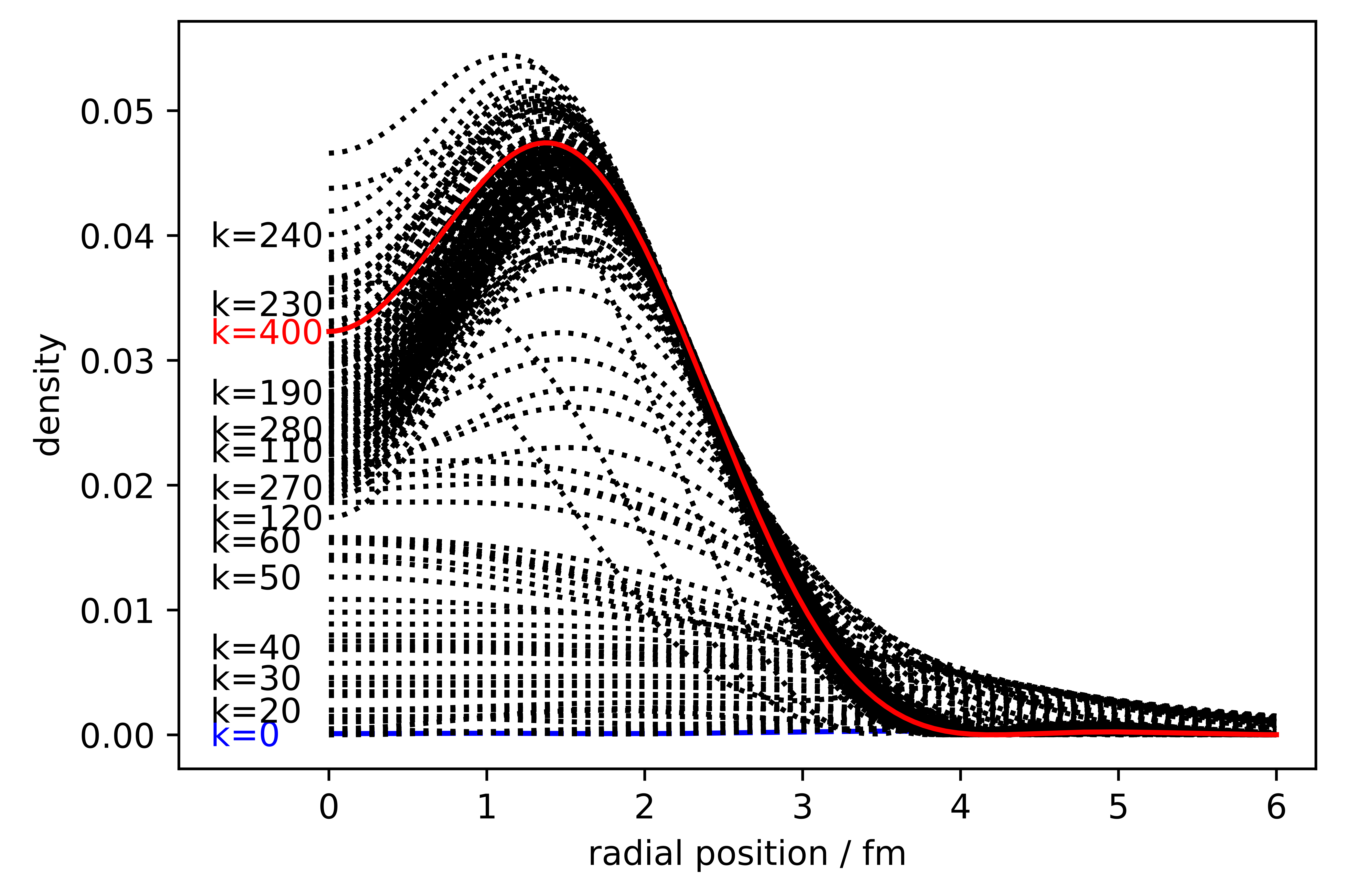
Figure 5: Quantum ITE for $N=3$ with 10000 shots.

Figure 4 and 5 show the evolution of the density as a function of iteration under the classical algorithm and quantum algorithm (10000 shots) respectively.

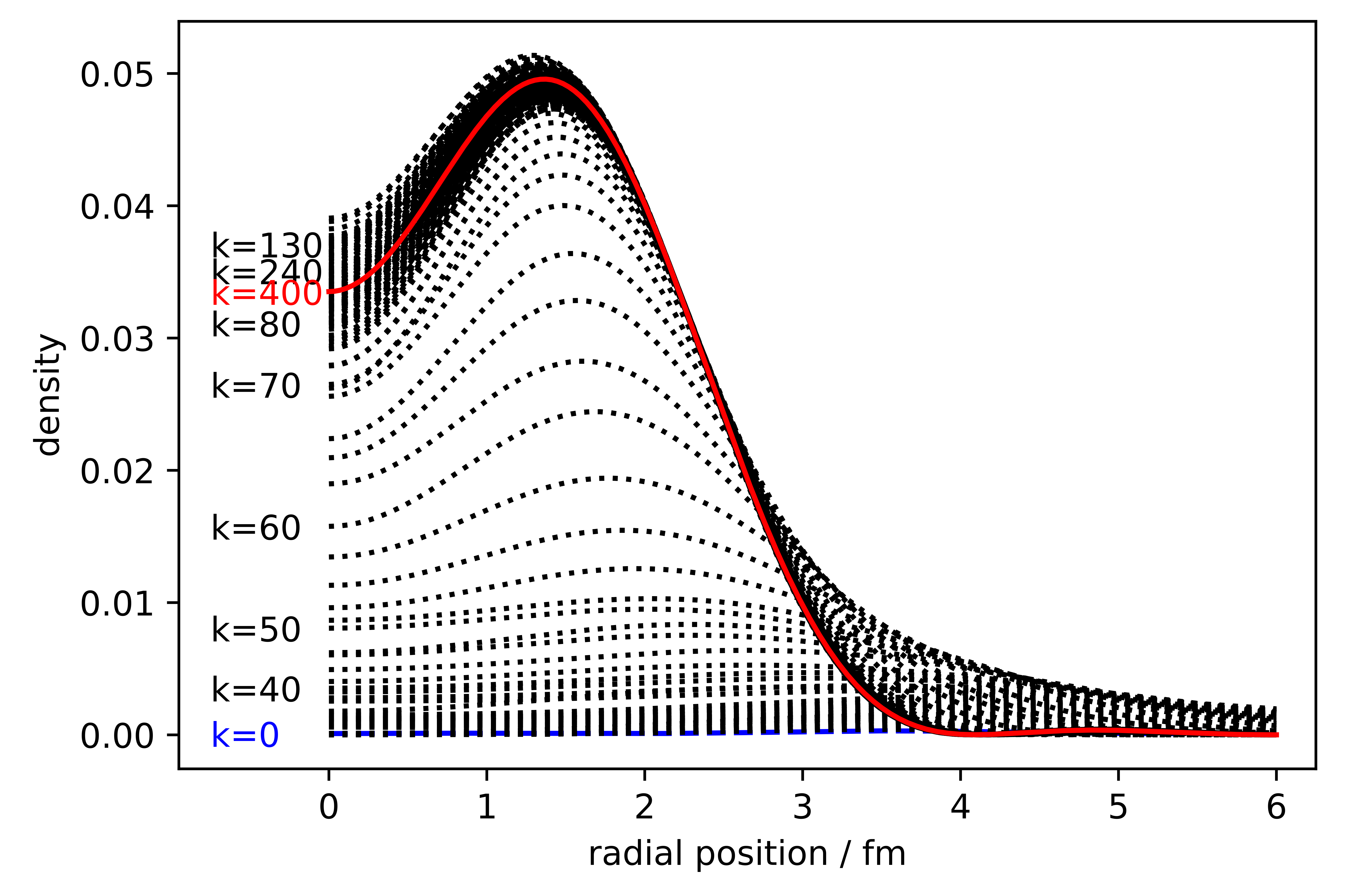
Figure 6: Quantum ITE for $N=3$ with 100000 shots.

Figure 6 shows the same quantum ITE with increased shots (100000 shots). Improvement of the unstable behaviour can be seen.

V.2 $N=4$ Case

The same behaviour appears in the $N=4$ case and affects more coefficients. With more coefficients failed to be measured in early time steps, the ITE of the state does not converge to the ground state.

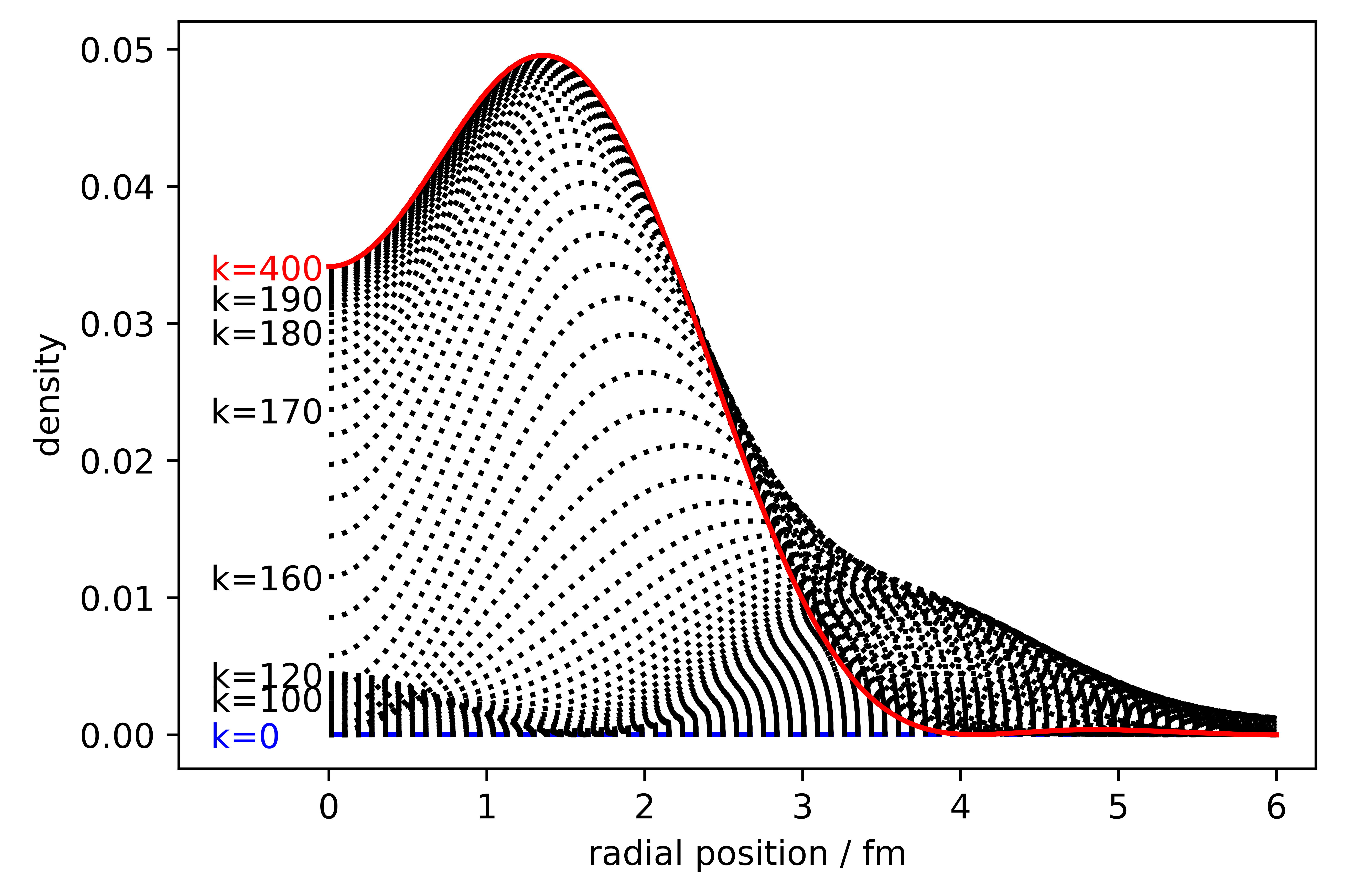
Figure 7: Classical ITE for $N=4$.

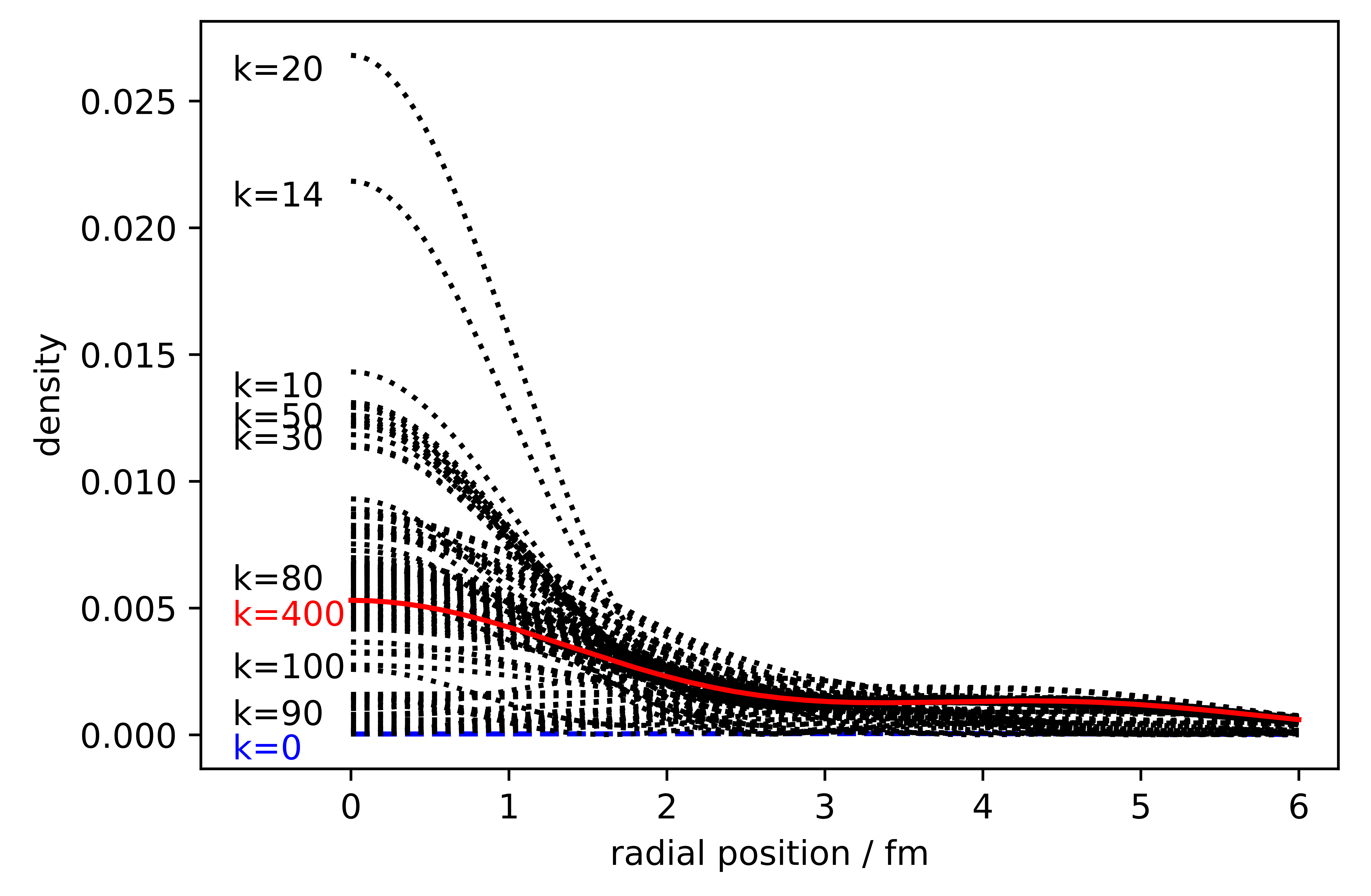
Figure 8: Quantum ITE for $N=4$ with 10000 shots.

Figure 7 and figure 8 show the difference between the expected and actual behaviour of the algorithm. Since our work are implemented using a quantum simulator instead of a real quantum hardware, increasing the number of shots for the $N=4$ is not plausible due to computational time. We instead run the simulation on the statevector backend from QISKIT [25].

Figure 9: Quantum ITE for $N=4$ using statevector simulator.

The results of this simulation is shown in figure 9. The per-iteration results and the ground state energy calculation are in close agreement with the classical algorithm.

VI Conclusion

We have presented an algorithm solving coupled non-linear Schrödinger equations via the imaginary time evolution method. Using Hartree-Fock equations for the oxygen-16 nucleus as an example, we show that this implementation provides results in agreement with the classical algorithm.

With a larger basis, our current algorithm faces its limitation. Some of the coefficients failed to be detected with our number of measurements. We show, with a statevector simulation, that the limitation lies not within the circuit but the measurements.

In the $N=3$ case this is improved by increasing the number of shots. Techniques to mitigate low probability of shots leading to useful measurements have been enacted in other related methods of implementing the quantum imaginary time method [26]. Such a technique cannot immediately be applied in our case due to our imaginary-time-dependent potential caused by the non-linear Schrödinger equation. However, a similar method might be possible.

Another possible solution is to increase the imaginary time step. A larger time step would result in more apparent changes in the coefficient values between iterations. This could prevent the state from being trapped in a local minima. However, with a larger time step the error from certain approximations (equations (4) and (8)).

Appendix A State Preparation Subcircuits

Denoting the $2^{\mathfrak{N}}$ coefficients in a $\mathfrak{N}$-qubit real state as $\{c_{i}\}$, $i=0,1,\dots,2^{\mathfrak{N}}-1$, the $\mathfrak{N}$-qubit state preparation subcircuit $SP(\mathfrak{N})$ is given in figure 10,

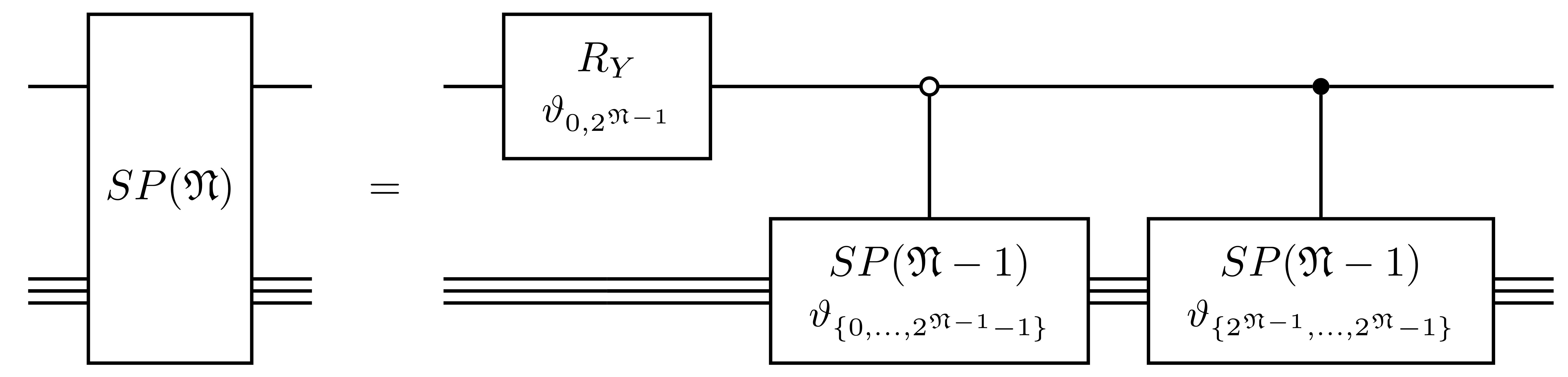
Figure 10: $\mathfrak{N}$-qubit real state preparation.

where the angles of rotation, $\vartheta_{ij}$, for the state preparation, are given by

$$\tan{\frac{\vartheta_{ij}}{2}}=\sqrt{\frac{\sum_{i^{\prime}=j}^{2j-i-1}c_{i^{\prime}}^{2}}{\sum_{i^{\prime}=i}^{j-1}c_{i^{\prime}}^{2}}}\text{,}$$ (20)

and $SP(1)$ is given in figure 11.

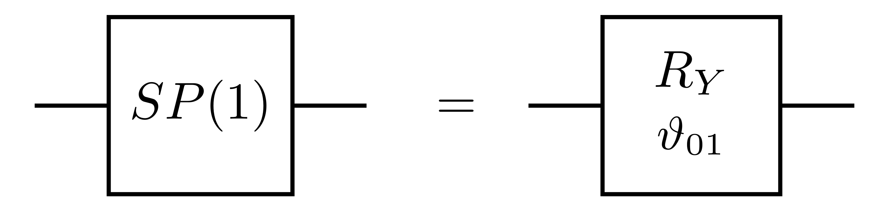
Figure 11: 1-qubit real state preparation.

References

- Feynman [1982] R. P. Feynman, Simulating physics with computers, Int. J. Theor. 21, 467 (1982).
- McArdle et al. [2020] S. McArdle, S. Endo, A. Aspuru-Guzik, S. C. Benjamin, and X. Yuan, Quantum computational chemistry, Rev. Mod. Phys. 92, 015003 (2020).
- Cao et al. [2019] Y. Cao, J. Romero, J. P. Olson, M. Degroote, P. D. Johnson, M. Kieferová, I. D. Kivlichan, T. Menke, B. Peropadre, N. P. D. Sawaya, S. Sim, L. Veis, and A. Aspuru-Guzik, Quantum chemistry in the age of quantum computing, Chemical Reviews 119, 10856 (2019).
- Kim et al. [2023] Y. Kim, A. Eddins, S. Anand, K. X. Wei, E. van den Berg, S. Rosenblatt, H. Nayfeh, Y. Wu, M. Zaletel, K. Temme, and A. Kandala, Evidence for the utility of quantum computing before fault tolerance, Nature 618, 500 (2023).
- Arute et al. [2020] F. Arute, K. Arya, R. Babbush, D. Bacon, J. C. Bardin, R. Barends, S. Boixo, M. Broughton, B. B. Buckley, D. A. Buell, B. Burkett, N. Bushnell, Y. Chen, Z. Chen, B. Chiaro, R. Collins, W. Courtney, S. Demura, A. Dunsworth, E. Farhi, A. Fowler, B. Foxen, C. Gidney, M. Giustina, R. Graff, S. Habegger, M. P. Harrigan, A. Ho, S. Hong, T. Huang, W. J. Huggins, L. Ioffe, S. V. Isakov, E. Jeffrey, Z. Jiang, C. Jones, D. Kafri, K. Kechedzhi, J. Kelly, S. Kim, P. V. Klimov, A. Korotkov, F. Kostritsa, D. Landhuis, P. Laptev, M. Lindmark, E. Lucero, O. Martin, J. M. Martinis, J. R. McClean, M. McEwen, A. Megrant, X. Mi, M. Mohseni, W. Mruczkiewicz, J. Mutus, O. Naaman, M. Neeley, C. Neill, H. Neven, M. Y. Niu, T. E. O’Brien, E. Ostby, A. Petukhov, H. Putterman, C. Quintana, P. Roushan, N. C. Rubin, D. Sank, K. J. Satzinger, V. Smelyanskiy, D. Strain, K. J. Sung, M. Szalay, T. Y. Takeshita, A. Vainsencher, T. White, N. Wiebe, Z. J. Yao, P. Yeh, and A. Zalcman, Hartree-fock on a superconducting qubit quantum computer, Science 369, 1084 (2020).
- Vorwerk et al. [2022] C. Vorwerk, N. Sheng, M. Govoni, B. Huang, and G. Galli, Quantum embedding theories to simulate condensed systems on quantum computers, Nature Computational Science 2, 424 (2022).
- Bassman et al. [2021] L. Bassman, M. Urbanek, M. Metcalf, J. Carter, A. F. Kemper, and W. A. d. Jong, Simulating quantum materials with digital quantum computers, Quantum Science and Technology 6, 043002 (2021).
- Višňák [2015] J. Višňák, Quantum algorithms for computational nuclear physics, EPJ Web of Conferences 100, 01008 (2015).
- Zhang et al. [2021] D.-B. Zhang, H. Xing, H. Yan, E. Wang, and S.-L. Zhu, Selected topics of quantum computing for nuclear physics, Chinese Physics B 30, 020306 (2021).
- Stevenson [2023] P. D. Stevenson, Comments on Quantum Computing in Nuclear Physics, International Journal of Unconventional Computing 18, 83 (2023).
- García-Ramos et al. [2023] J. E. García-Ramos, A. Sáiz, J. M. Arias, L. Lamata, and P. Pérez-Fernández, Nuclear Physics in the Era of Quantum Computing and Quantum Machine Learning (2023), arXiv:2307.07332.
- Li et al. [2023] Y. H. Li, J. Al-Khalili, and P. Stevenson, A quantum simulation approach to implementing nuclear density functional theory via imaginary time evolution (2023), arXiv:2308.15425 [nucl-th] .
- Lehtovaara et al. [2007] L. Lehtovaara, J. Toivanen, and J. Eloranta, Solution of time-independent schrödinger equation by the imaginary time propagation method, J. Comput. Phys. 221, 148 (2007).
- Suzuki [1976] M. Suzuki, Generalized trotter’s formula and systematic approximants of exponential operators and inner derivations with applications to many-body problems, Commun. Math. Phys. 51, 183 (1976).
- Wu et al. [1999] J.-S. Wu, M. R. Strayer, and M. Baranger, Monopole collective motion in helium and oxygen nuclei, Physical Review C 60, 044302 (1999).
- Skyrme [1959] T. Skyrme, The effective nuclear potential, Nucl. Phys. 9, 615 (1958-1959).
- Dobaczewski and Dudek [1997] J. Dobaczewski and J. Dudek, Solution of the skyrme-hartree-fock equations in the cartesian deformed harmonic oscillator basis i. the method, Comput. Phys. Commun. 102, 166 (1997).
- Davies et al. [1969] K. T. R. Davies, M. Baranger, R. M. Tarbutton, and T. T. S. Kuo, Brueckner-Hartree-Fock Calculations of Spherical Nuclei in an Harmonic-Oscillator Basis, Phys. Rev. 177, 1519 (1969).
- Welsh and Rowe [2016] T. Welsh and D. Rowe, A computer code for calculations in the algebraic collective model of the atomic nucleus, Comput. Phys. Commun. 200, 220 (2016).
- Lv et al. [2022] P. Lv, S.-J. Wei, H.-N. Xie, and G.-L. Long, QCSH: a Full Quantum Computer Nuclear Shell-Model Package (2022), arXiv: 2205.12087.
- Pesce and Stevenson [2021] R. M. N. Pesce and P. D. Stevenson, H2zixy: Pauli spin matrix decomposition of real symmetric matrices (2021).
- Gui-Lu [2006] L. Gui-Lu, General Quantum Interference Principle and Duality Computer, Commun. Theor. Phys. 45, 825 (2006).
- Wei et al. [2020] S. Wei, H. Li, G. Long, and G. Long, A full quantum eigensolver for quantum chemistry simulations, Research 2020, 1 (2020).
- Plakhutin [2018] B. Plakhutin, Koopmans’ theorem in the Hartree-Fock method. General formulation, J. Chem. Phys. 148, 094101 (2018).
- Qiskit contributors [2023] Qiskit contributors, Qiskit: An open-source framework for quantum computing (2023), https://doi.org/10.5281/zenodo.8090426.
- Mangin-Brinet et al. [2023] M. Mangin-Brinet, J. Zhang, D. Lacroix, and E. A. R. Guzman, Efficient solution of the non-unitary time-dependent schrodinger equation on a quantum computer with complex absorbing potential (2023), arXiv:2311.15859 [quant-ph] .