NeuroCine: Decoding Vivid Video Sequences from Human Brain Activties

Abstract

In the pursuit to understand the intricacies of human brain’s visual processing, reconstructing dynamic visual experiences from brain activities emerges as a challenging yet fascinating endeavor. While recent advancements have achieved success in reconstructing static images from non-invasive brain recordings, the domain of translating continuous brain activities into video format remains underexplored. In this work, we introduce NeuroCine, a novel dual-phase framework to targeting the inherent challenges of decoding fMRI data, such as noises, spatial redundancy and temporal lags. This framework proposes spatial masking and temporal interpolation-based augmentation for contrastive learning fMRI representations and a diffusion model enhanced by dependent prior noise for video generation. Tested on a publicly available fMRI dataset, our method shows promising results, outperforming the previous state-of-the-art models by a notable margin of ${20.97\%}$, ${31.00\%}$ and ${12.30\%}$ respectively on decoding the brain activities of three subjects in the fMRI dataset, as measured by SSIM. Additionally, our attention analysis suggests that the model aligns with existing brain structures and functions, indicating its biological plausibility and interpretability.

1 Introduction

Human experiences are inherently dynamic, unfolding moment by moment much like frames in a movie (Varela et al., 2017). The human brain, with its extraordinary complexity, continuously interprets these visual stimuli, weaving a rich tapestry of experiences (Bartels et al., 2008; Nishimoto et al., 2011). Unraveling the intricacies of this complex system to understand the neural activities beneath remains a remarkable challenge. One of the most ambitious endeavors in this field is the reconstruction of these dynamic visual experiences using non-invasive brain measures (Kupershmidt et al., 2022; Chen et al., 2023; Wang et al., 2022). Successfully achieving this could not only aid people with disabilities but also deepen our understanding of dynamic vision processing mechanisms in the human brain.

Functional Magnetic Resonance Imaging (fMRI), noted for its high spatial resolution, is pivotal in capturing detailed activations within the visual cortex and related brain areas (Hénaff et al., 2021). This aspect is particularly advantageous for reconstructing visual content from brain activity. While there has been significant progress in reconstructing static images (Chen et al., 2022; Sun et al., 2023a), video reconstruction remains an area under active exploration. Challenges arise from fMRI’s inherent characteristics: it primarily measures changes in the blood-oxygen-level-dependent (BOLD) signal, showing spatial redundancy in adjacent voxels (Uğurbil et al., 2013). Additionally, a temporal lag exists between neural activity and BOLD signals due to hemodynamic response, potentially causing discrepancies between visual stimuli and their fMRI representations (de Zwart et al., 2009). Furthermore, the non-invasive nature of fMRI introduces noise from various physiological and scanner-related sources (Parrish et al., 2000), complicating high-fidelity video reconstruction.

In response to these challenges, we propose a dual-phase framework namely NeuroCine to reconstruct high-resolution videos from fMRI data. Targeting the special spatial-temporal characteristics of fMRI, we propose to augment fMRI with spatial masking and temporal interpolation in the first phase. An fMRI encoder is optimized to learn representations robust against the disturbances caused by the augmentation. Building on this, the second phase employs the trained fMRI encoder to guide a video diffusion model in generating videos. We enhance this phase by incorporating dependent prior noise to address fMRI’s low signal-to-noise ratio. With these two key innovations, our double-phase approach aims to effectively translate complex and noisy fMRI data into accurate and meaningful visual reconstructions, demonstrating the synergy between advanced neural imaging and machine learning in decoding brain activity.

We evaluate our method using a publicly available fMRI-video pair dataset from three human subjects watching videos. Our results significantly outperform previous models in both pixel-level and semantic-level metrics. Specifically, our method surpasses the previous SOTA model (Chen et al., 2023) by a notable margin of $\mathbb{20.97\%}$ in decoding brain activities of Subject 1, $\mathbb{31.00\%}$ in Subject 2, and $\mathbb{12.30\%}$ in Subject 3. Additionally, attention analysis of our model reveals correlations with the visual cortex and higher cognitive networks, indicating biological plausibility and interpretability. This underlines the potential of our method in advancing the field of neural decoding and visual reconstruction.

2 Related Works

2.1 Decoding Visual Contents from Brain Activities

Reconstructing Images from Brain Activities

The advancement of deep generative models (Fang et al., 2021) has catalyzed research in reconstructing visual content from brain activities. This area has predominantly focused on decoding both viewed and imagined images. Initially, many studies converted fMRI signals into image features, which were then used by fine-tuned GANs to generate images (Mozafari et al., 2020; Seeliger et al., 2017). For instance, (Shen et al., 2019) utilized a pre-trained VGG network to decode fMRI data into hierarchical image features, which were subsequently input into a GAN for image synthesis. More recent works over the past two years have shifted towards using Diffusion Models, which have produced images that are more semantically coherent and visually realistic (Qian et al., 2023; Lin et al., 2022; Chen et al., 2022; Sun et al., 2023a). For example, (Sun et al., 2023b) enhanced fMRI representation learning with denoising techniques and integrated pixel-level guidance from image auto-encoders, effectively separating vision-related neural activities from background noise.

Reconstructing Videos from Brain Activities Though studies reconstructing static images from brain activities keep emerging, decoding videos remains a challenging task under exploration. Conventional methods for video reconstruction from fMRI data typically approached the task as a sequence of separate image reconstructions. As noted by (Wen et al., 2018), this could lead to lower frame rates and a lack of consistency across frames. Despite these limitations, their research demonstrated the feasibility of decoding both low-level image features and categorical information from fMRI data in response to video stimuli. Building on this, (Wang et al., 2022) employed a linear layer to encode fMRI representations and utilized a conditional video GAN to enhance the quality and frame rate of the generated videos. Nonetheless, the effectiveness of this method is limited by a limited dataset, which is a significant challenge considering the substantial data demands of GAN training.

Similar to what (Beliy et al., 2019) had done, (Kupershmidt et al., 2022) applied a separable autoencoder conducive to self-supervised learning, managing to surpass the outcomes of (Wang et al., 2022). However, the visual quality and semantic accuracy of the resulting videos remained suboptimal. Advancing the field, (Chen et al., 2023) introduced the use of contrastive learning alongside spatial-temporal attention mechanisms to effectively learn the fMRI representation. Though they also targeted the spatial-temporal features of fMRI with such attention, they did not train the model itself to be robust to spatial and temporal disturbances as we do. They also only used the naive diffusion setup while we introduce dependent noise considering the noisy nature of fMRI. Methods from (Kupershmidt et al., 2022; Chen et al., 2023; Wang et al., 2022) will serve as baselines in this paper and be compared against our proposed method.

2.2 Diffusion Models

Diffusion Models (Ho et al., 2020), drawing inspiration from nonequilibrium thermodynamics, are probabilistic models that transform data into Gaussian noise and then back to the original data, showcasing exceptional performance in content generation tasks such as text to image (Rombach et al., 2022), 3D object (Poole et al., 2022), and audio generation (Chen et al., 2020). The iterative nature of these models, requiring hundreds of steps for generation, has been addressed by Song et al. (2020) with the denoising diffusion implicit model (DDIM), reducing the number of steps for high-quality outputs. Enhancements like ordinary differential equation solvers (Lu et al., 2022a, b; Liu et al., 2022), variance optimization (Bao et al., 2022), exposure bias reduction (Li et al., 2024; Ning et al., 2024, 2023), and improved noise schedulers (Nichol & Dhariwal, 2021) further accelerate inference and refine generative capabilities.

2.3 Video Generation with Diffusion Models

The initial advancements of using Diffusion Models to generate videos are primarily attributed to the work of VDM (Ho et al., 2022b) which introduced the 3D diffusion UNet. A subsequent development by Ho et al. (2022a) used a cascaded sampling framework with a super-resolution method to generate high-resolution videos. Further contributions in this realm include the introduction of a temporal attention mechanism over frames by Singer et al. (2022) in Make-A-Video. MagicVideo by Zhou et al. (2022) and (He et al., 2022) LVDM incorporate this mechanism within the latent Diffusion Models to generate videos. In this work, we adapt the image diffusion model to video diffusion model by inserting a temporal layer after each spatial layer and incorporating dependent noises.

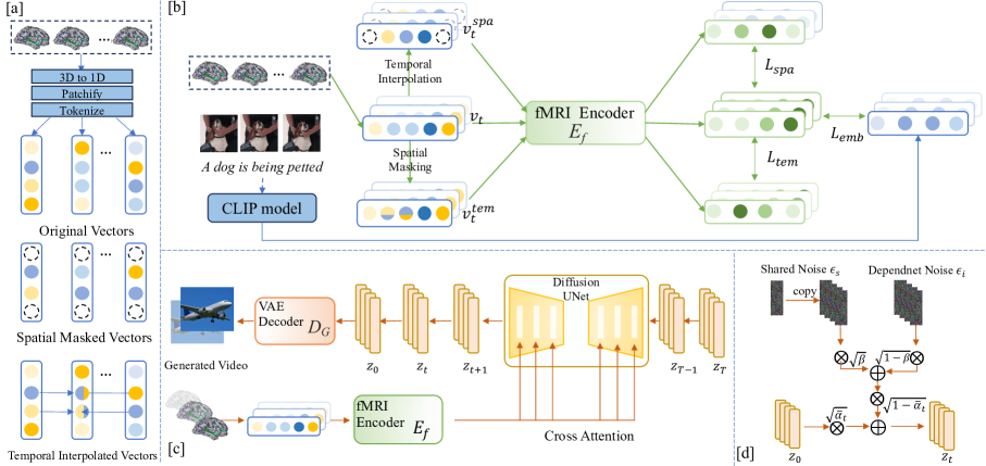
Figure 1: The proposed double-phase framework to reconstruct seen videos from fMRI. [a]: Using spatial masking and temporal interpolation to produce augmented samples [b]: Phase 1 trains an fMRI encoder to map from fMRI to CLIP text and image embeddings with contrastive learning. [c]: Phase 2 conditions generation of a diffusion model with Phase 1’s fMRI encoder incorporating dependent noises. [d]: Dependent noise generation.

3 Method

Our method consists of fMRI feature leaning and video decoding two-phase framework for reconstructing videos from fMRI-recorded brain activities. Phase 1 involves tuning a pre-trained fMRI encoder with spatial and temporal augmented contrastive learning to align fMRI data with CLIP’s text and image features, enhancing the extraction of semantic information from fMRI signals. Phase 2 uses the trained fMRI encoder to guide a video diffusion model, incorporating dependent prior noise to compensate for fMRI’s low signal-to-noise ratio.

In Section 3.1, we delve into learning fMRI representation with spatial and temporal augmented contrastive learning. In Section 3.2, we elaborate on the design of prior noise for the video diffusion model to decode more coherent videos from brain activity. In Section 3.3, we describe our experimental approach for analyzing our results, aiming to clarify the contribution of each brain region throughout different stages of learning.

3.1 FMRI Feature Learning

3.1.1 Pre-training and FMRI Input Format

Pre-training

The scarcity of fMRI-video pair data compels us to leverage a pre-trained fMRI representation space, a strategy widely acknowledged by prior research (Sun et al., 2023b; Chen et al., 2023, 2022; Sun et al., 2023a). We utilize a model shared by Sun et al. (2023b), which has been effectively applied in image reconstruction from fMRI. This model benefits from a double-contrastive masked autoencoding (DC-MAE) technique, optimized on the HCP dataset (Van Essen et al., 2013). It incorporates a Vision Transformer-based encoder to process masked fMRI signals and a decoder dedicated to restoring the original, unmasked signals. The term “Double-Contrastive” underlines the model’s strategy of employing two distinct contrasting operations to optimize contrastive losses during fMRI representation learning. We adopt this fMRI encoder to establish a pre-trained representation space. For further details on this methodology, we recommend consulting the original publication.

FMRI Input Format In our video decoding approach, we view fMRI data as a sequence of 3D tensors, but due to the limited scale of fMRI-video pairs, we avoid complex, heavily parameterized models for capturing the 3D structure of fMRI. Considering previous work with satisfactory decoding performance (Sun et al., 2023b; Chen et al., 2022), the fMRI data from the visual cortex is rearranged from 3D to 1D, aligned with the visual processing hierarchy, segmented into uniform patches, and then converted into tokens. Traditional methods of neural decoding often oversimplify the translation of fMRI data into video frames by mapping fMRI frames to a fixed number of frames, creating an “fMRI frame window”. However, this approach does not adequately address the temporal delay in fMRI data. To overcome this, we implement a sliding window, defined as $\boldsymbol{v}_{\boldsymbol{t}}=\left\{v_{t},v_{t+1},\ldots,v_{t+w-1}\right\}$, with $v_{t}\in\mathbb{R}^{n\times p\times b}$ representing token embeddings at time $t$, where $n$, $p$, and $b$ denote batch size, patch size, and embedding dimension. This results in $\boldsymbol{v}_{\boldsymbol{t}}\in\mathbb{R}^{n\times w\times p\times b}$, where $w$ is the window size. We then apply our algorithms to these windows, considering the unique spatiotemporal characteristics of fMRI, as elaborated in subsequent subsections.

3.1.2 Spatial and Temporal Augmentation

To address the challenges of limited fMRI-video pair availability and the low signal-to-noise ratio in fMRI data, we propose a noise-robust fMRI encoder training method. A key aspect of our method is the novel cognitive plausible augmentation of samples for contrastive learning, adapted to the unique spatial and temporal features of fMRI data. Traditional computer vision augmentation techniques like cropping and rotation are not ideally suitable for fMRI data. FMRI images capture brain activity with spatial specificity tied to neurological function. Rotating or cropping these images could disrupt the inherent functional topology. After a thorough literature review (Glover, 2011; Buxton, 2009) and expert consultations, we employ two effective augmentation methods: spatial masking and temporal interpolation.

For spatial masking, we randomly select a portion of the tokens and set them to zero. Formally, in $\boldsymbol{v}_{\boldsymbol{t}}\in\mathbb{R}^{n\times w\times p\times b}$, we set $\gamma_{spa}b$ values in the fourth dimension of shape $b$ to zero, with $\gamma_{spa}$ as a hyperparameter. The positions to be masked are consistent within the same window. But we do not force the masked positions to be uniform across the same batch.

Temporal interpolation replaces randomly selected frames within a window with interpolations of other frames, weighted by their temporal distance—the farther the frame, the lower its weight. Mathematically, for a window with $w$ fMRI frames $\boldsymbol{v}_{\boldsymbol{t}}$, and the selected $i^{th}$ frame ${v_{t_{i}}}$, the jittered frame $\hat{v_{t_{i}}}$ is calculated as:

$$\hat{v_{t_{i}}}=\sum\limits_{j=1,j\neq i}^{n}\left(1-\frac{\lvert i-j\rvert}{n}\right)v_{t_{j}}$$ (1)

The original frame $v_{t_{i}}$ will then be replaced by $\hat{v}_{t_{i}}$. The extent of interpolation is controlled by the temporal interpolation ratio $\gamma_{tem}$, a hyperparameter. The setting and effects of $\gamma_{tem}$ and $\gamma_{spa}$ will be detailed in Section 5.2 Ablation Study.

3.1.3 Contrastive Mapping

In our method, we employ a vision-Transformer-based fMRI encoder to process fMRI token vectors, aligning them with the CLIP model’s text and image embeddings. This process is enhanced by incorporating contrastive learning using augmented examples as described in the previous subsection.

Initially, we utilize the pre-trained CLIP model (Radford et al., 2021) to encode the stimuli used in the collection of fMRI data. For each video, captions are generated using the pre-trained BLIP model (Li et al., 2022) and then encoded with the CLIP model to produce text embeddings. Similarly, we process each video frame to generate corresponding image embeddings. The fMRI encoder is fed with the token vectors and trained to map from fMRI to CLIP embeddings. Additionally, the fMRI encoder is fed with both the spatially and temporally augmented examples and is optimized with contrastive losses to learn fMRI features robust to the spatial and temporal disturbances.

The formal representation of our loss functions, considering the original fMRI token vectors $\boldsymbol{v}_{\boldsymbol{t}}$, their spatially augmented version $\boldsymbol{v}_{\boldsymbol{t}}^{spa}$, and temporally augmented version $\boldsymbol{v}_{\boldsymbol{t}}^{tem}$, is as follows:

$$L_{spa}= L_{CE}[E_{f}(\boldsymbol{v}_{\boldsymbol{t}}),E_{f}(\boldsymbol{v}_{\boldsymbol{t}}^{tem})]$$ (2)

$$L_{tem}= L_{CE}[E_{f}(\boldsymbol{v}_{\boldsymbol{t}}),\>E_{f}(\boldsymbol{v}_{\boldsymbol{t}}^{spa})]$$

$$L_{emb}= L_{CE}[E_{f}(\boldsymbol{v}_{\boldsymbol{t}}),\>e^{txt}_{t}]+L_{CE}[E_{f}(\boldsymbol{v}_{\boldsymbol{t}}),\>e^{img}_{t}],$$

where $L_{CE}$ is the cross-entropy loss and $E_{f}$ denotes the fMRI encoder. $e^{txt}_{t}$ and $e^{img}_{t}$ mean the CLIP text and image embeddings. We aim to optimize these losses jointly, with the overall loss function being defined as:

$$L_{E_{f}}=\mu_{spa}L_{spa}+\mu_{tem}L_{tem}+L_{emb}$$ (3)

In this equation, $\mu_{spa}$ and $\mu_{tem}$ are hyperparameters that adjust the weight of the corresponding losses. The setting and effects of $\mu_{spa}$ and $\mu_{tem}$ will be detailed in Section 5.2.

3.2 Generation with Diffusion Model

3.2.1 Prelimiaries

Diffusion Models (Sohl-Dickstein et al., 2015) show significant potential in generating both images and videos. In this work, we adopt the widely used Stable Diffusion (SD) (Rombach et al., 2022) as the baseline model, known for its efficient denoising capabilities in the image’s latent space, which requires considerably fewer computational resources. During training, the SD begins by using a KL-VAE (Kingma & Welling, 2013) encoder to convert image $x_{0}$ to latent space: $z_{0}=\mathcal{E}(x_{0})$. It then progressively transforms this latent representation into a Gaussian noise, following the equation:

$$z_{t}=\sqrt{\bar{\alpha}_{t}}z_{0}+\sqrt{1-\bar{\alpha}_{t}}\epsilon$$ (4)

Here, the $\epsilon$ represents a noise sampled from a normal distribution: $\epsilon\sim\mathcal{N}(0,1)$. $\bar{\alpha}_{t}$ is the predefined noise schedule. The model is trained to predict the added noise at each step, and the loss function could be formulated as :

$$\mathcal{L}_{t}^{simple}=E_{t,x_{0},\epsilon_{t}\sim\mathcal{N}(0,1)}[\|\epsilon_{t}-\epsilon_{\theta}(z_{t},t,c)\|_{2}^{2}]$$ (5)

$t$ is the diffusion time step, and $c$ is the text prompt condition. During inference, the SD gradually reconstructs an image aligned with the provided text prompt from Gaussian noise. The denoised results are then processed through the decoder of the KL-VAE to reconstruct the colored images from their latent representation: $x_{0}=\mathcal{D}(z_{0})$.

3.2.2 Dependent Prior Video Diffusion.

Following previous studies (Wu et al., 2023; Chen et al., 2023), we utilize a pre-trained text-to-image Stable Diffusion (SD) model as our foundational video generator. While adept at creating high-quality individual frames, the original SD model lacks temporal coherence for video generation. To address this, we modify it by converting 2D convolutions to pseudo 3D and adding a temporal attention layer after each spatial self-attention layer. This modification introduces temporal awareness, allowing each visual token to attend to tokens from the previous two frames. The temporal attention layer operates as:

$$Attention(Q,K,V)=Softmax(\frac{QK^{T}}{\sqrt{d_{k}}})V$$ (6)

with $Q,K,V$ being the query, key, and value matrices, and $W^{Q},W^{K},W^{V}$ as learnable parameters.

For decoding brain activity into video, we start by sampling $m$ latent codes from Gaussian noise and progressively refine them using the fMRI representation. Given the low signal-to-noise ratio in fMRI signals, enhancing video quality is challenging. Previous research (Ge et al., 2023) demonstrates that employing a deterministic ODE solver in the generative process of the SD model results in a high correlation of initial noise in frames from the same video. Similarly, it has been observed that fMRI signals from similar visual stimuli exhibit a high degree of correlation. Based on these observations, we utilize correlated noise as a form of prior knowledge within the generative model and the fMRI decoding process. To create a sequence of dependent noise, where each noise is sampled from Gaussian Distribution with a mean of zero and a variance of one, we divide each noise into two components: $\epsilon_{s}$ and $\epsilon_{i}^{j}$, and the dependent noise is obtained by following formula:

$$\epsilon^{j}=\sqrt{\beta}\cdot\epsilon_{s}+\sqrt{1-\beta}\cdot\epsilon_{i}^{j}$$ (7)

where $\epsilon_{s}\sim\mathcal{N}(0,1)$ and $\epsilon_{i}\sim\mathcal{N}(0,1)$. $\sqrt{\beta}$ is the hyperparameter conditioning the noise ratio, whose setting and effects are discussed in Section 5.2’s Ablation Study. A visualization of generating dependent noise is presented in Figure 1 [d]. During training, we substitute the original noise in SD model with our customized dependent noise to generate noisy latent codes at each time step. Conversely, in the generative phase, the process begins with the introduction of our dependent noise.

3.3 Interpretation of Brain Activity

Understanding the activated brain regions is another significant objective in brain encoding and decoding work. In this study, we analyze the results using the self-attention mechanism within the fMRI encoder for each fMRI-video pair. The attention maps are visualized at various stages of model learning, across different layers, and in response to different visual stimuli. This approach helps in elucidating the contribution of each brain region across various learning stages.

Initially, a sample-level interpretation is conducted. For each fMRI-video sample pair, we extract self-attention maps from three key layers in the fMRI encoder: the early layer (the first layer), the middle layer (the 12th layer), and the final layer (the 24th layer). These attention maps are then averaged across all video samples to facilitate a group-level analysis. To correlate the attention values with specific brain regions, we reverse-engineer the patchified fMRI data back into fMRI voxels using the inverse computation of the FC layer. Subsequently, these fMRI voxels are mapped onto the selected Regions of Interest (ROIs) on the CIFITI den-91k surface, as referenced in (Van Essen et al., 2013). For visualization purposes, we employ Nilearn (Abraham et al., 2014) to plot the brain voxels back to the brain surface to enhance our understanding of complex brain activities.

4 Experimental Setup

4.1 Dataset

Our study uses a publicly accessible fMRI-video dataset, cited as dataset (Wen et al., 2018), which includes both fMRI and video clip data. The fMRI data were captured using a 3T MRI scanner with a 2-second repetition time (TR) and involved three participants. The dataset comprises a training set of 18 video clips, each 8 minutes long, totaling 2.4 hours and providing 4,320 paired training examples. The testing set includes 5 sections of 8-minute video clips, totaling 40 minutes, resulting in 1,200 test fMRI scans. These videos, displayed at 30 FPS, feature diverse content including animals, humans, and natural landscapes.

4.2 Evaluation Metric

Our evaluation metrics are divided into pixel-level and semantics-level assessments. For pixel-level, we use the Structural Similarity Index Measure (SSIM) (Wang et al., 2004). For semantics-level, we employ an N-way top-K accuracy classification test. Both SSIM and classification accuracy are computed for each frame against its groundtruth frame. The classification test involves an ImageNet classifier comparing the classifications of the groundtruth and predicted frames. Success is defined when the groundtruth class ranks within the top-K probabilities of the predicted frame’s classification from N randomly chosen classes, including the groundtruth itself. This test is repeated 100 times to calculate an average success rate.

For video-based metrics, a similar classification approach is used but with a video classifier. This classifier, based on VideoMAE (Tong et al., 2022) and trained on the Kinetics-400 dataset (Kay et al., 2017), assesses video semantics across 400 categories, including various motions and human interactions.

4.3 Implementation Details

For a fair comparison with previous SOTA (Chen et al., 2023), the original videos in our study are reduced in frame rate from 30 frames per second (FPS) to 3 FPS and the window size is set as 2. This results in a conversion where each fMRI frame corresponds to six video frames. In our practical application, this approach enables the reconstruction of a 2-second video segment (consisting of six frames) from a single fMRI frame. Our method is capable of generating the reconstruction of longer video sequences from multiple fMRI frames, contingent on the availability of additional GPU memory.

For the first phase, our implementation utilizes a Vision Transformer (ViT)-based fMRI encoder. We employ a fMRI encoder pre-trained on large-scale public available fMRI data by previous work (Sun et al., 2023b). This encoder is characterized by the following parameters: a patch size of 16, a depth of 24 layers, and an embedding dimension of 1024. Initially, the encoder undergoes pre-training with a mask ratio of 0.75. Subsequently, it is enhanced with the addition of a projection head. This projection head serves to transform the token embeddings into a dimensionality of 77×768. Settings of hyperparameters related with spatial and temporal augmentation are discussed in Section 5.2.

In the second phase, our approach involves leveraging Stable Diffusion V1-5 (Rombach et al., 2022). Although the initial version of Stable Diffusion is trained for processing images at a resolution of $512\times 512$, our experimental methodology involves fine-tuning the model. This fine-tuning incorporates an augmented temporal layer, adapting the model for video processing at a reduced resolution of $256\times 256$ and a frame rate of 3 FPS. In this phase, we specifically focus on fine-tuning the parameters within the spatial attention, cross-attention, and temporal attention heads of the diffusion model. The training process is carried out with text conditioning for a duration of 1000 steps, utilizing a learning rate of $2\times 10^{-5}$ and a batch size of $14$. After acquiring the video diffusion model, we replace its text encoder with an fMRI encoder, which has been previously trained. Subsequently, we fine-tune the layers responsible for spatial self-attention, visual-fMRI cross-attention, and temporal attention within the video generation model and the fMRI encoder. This fine-tuning is conducted using the fMRI-Video pair dataset. We use a learning rate of $2\times 10^{-5}$ and a batch size of 24. All experiments were conducted using a single A100 GPU.

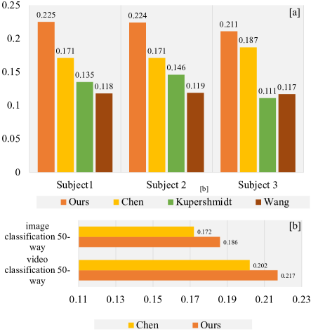
Figure 2: Comparisons of Structural Similarity Index Measure (SSIM) Scores and 50-way Image/Video Classification Accuracy. [a] Comparing the SSIM scores of our method with other three benchmarks on Subject 1, 2 and 3. (b) Comparing our method’s 50-way Image and Video Classification Accuracy with previous SOTA model on Subject 1.

5 Results

5.1 Video Reconstruction Performance

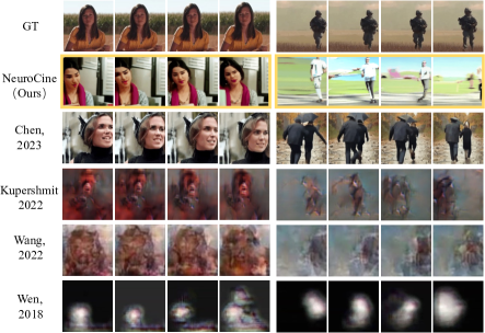
Figure 3: Comparison of the decoded results considering our framework NeuroCine and baselines.

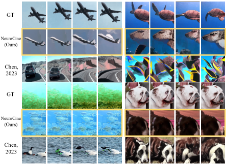
Figure 4: Additional comparisons of decoded results between our method NeuroCine and the previous state-of-the-art (SOTA) model.

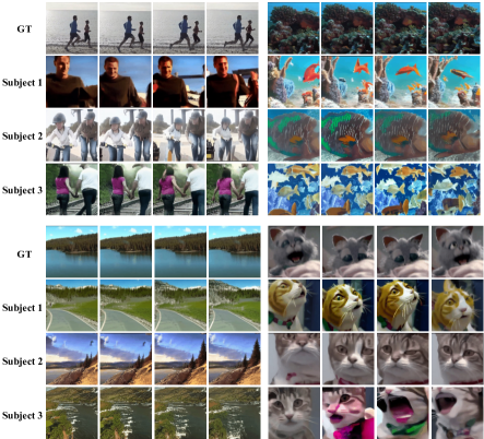
Figure 5: Decoded results of our framework NeuroCine from all three subjects in the dataset.

Table 1: Ablation study about NeuroCine’s important hyperparameters’ effects on final video decoding performance measured by SSIM, including spatial mask ratio, temporal interpolation ratio, spatial loss weight, temporal loss weight, using of dependent noise and dependent noise ratio.

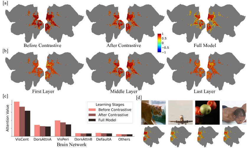
Figure 6: Self-Attention Analysis for Subject 1. The gradation from blue to red on the voxel map signifies the ascending importance of each voxel in the generation process, as determined by the attention analysis. Panels [a] and [c] emphasize the evolution of attention maps throughout the learning stages. Panel [b] highlights the differential attention patterns across various transformer layers. Panel [d] presents a comparative view of attention maps corresponding to a few video frame examples under different categories.

In this section, we compare our methodology with prior works, including studies from Chen et al. (2023), Wen et al. (2018), Wang et al. (2022), and Kupershmidt et al. (2022), focusing on Structural Similarity Index Measure (SSIM) scores and classification accuracy. Our SSIM results, shown in Figure 2 [a], indicate our method sets a new state-of-the-art (SOTA) with scores of $0.225$, $0.224$, and $0.211$ for Subject 1, 2, and 3. Specifically, our method surpasses the previous ( Chen et al. (2023)) by a significant margin of $\mathbb{20.97\%}$ in Subject 1, $\mathbb{31.00\%}$ in Subject 2 and $\mathbb{12.30\%}$ in Subject 3. (You may refer to hyperparamter settings in Table 1’s experiment 10 for reproduction of Subject 1’s decoding performance.) Figure 2 [b] further shows that our method achieves superior accuracy in both 50-way Image and Video Classification Accuracy.

Qualitative comparisons in Figure 3 show that, unlike other models that yield blurry or unrecognizable outputs, our method and Chen et al. (2023)’s approach produce high-quality, semantically accurate videos. A detailed comparison with the previous SOTA method (Chen et al. (2023)) in Figure 4 reveals our superior semantic alignment with ground truth videos. For instance, where our method accurately generates a video of a swimming turtle, Chen et al. (2023)’s output shows a group of fish. The versatility of our model is further demonstrated in Figure 5 which shows our model’s reconstructed results on all subjects, where it consistently decodes high-quality, semantically accurate videos from different subjects. We present more video frames generated by our model in Figure 7 in the appendix.

5.2 Ablation Study

In this subsection, we perform an ablation study to assess the impact of each component within our model and the significance of hyperparameter settings on video decoding performance.

Spatial and Temporal Augmentation: The ratios for spatial masking and temporal interpolation dictate the extent of modification to the fMRI token vectors to generate augmented samples. Results from experiments [0-3] in Table 1 indicate that spatial augmentation significantly enhances decoding performance, with a spatial mask ratio of 0.2 yielding the best results. However, excessive masking detrimentally affects the SSIM of the reconstructed samples, underscoring the balance needed to utilize fMRI’s spatial redundancy effectively. A similar balance is crucial for the temporal interpolation ratio, where a ratio of 1/3 enhances performance without the adverse effects seen when the ratio is increased further.

Augmentation Loss Weight: The augmentation loss weights determine their contribution to the total loss in optimizing the fMRI encoder. Experiments [1, 5-7] in Table 1 demonstrate that a balanced augmentation loss between spatial and temporal aspects improves performance, with setting both weights to 1 achieving the highest SSIM. This highlights the importance of evenly capturing spatial and temporal features of fMRI data for accurate video decoding.

Dependent Noise Ratio: Introducing dependent noise targets the inherent noise in fMRI data, enhancing the model’s ability to decode videos, as shown in experiments [1, 8-10] in Table 1. This could confirm our hypothesis that incorporating dependent noise as a prior enhances video reconstruction with Diffusion Models. However, we also observe that increasing the noise ratio ($\sqrt{\beta}$) too much can negatively affect performance. This outcome is anticipated, since a higher noise ratio results in each frame becoming more similar to the others, leading to the creation of videos with frames that are too closely aligned, lacking variation and dynamism, and potentially resulting in nearly static videos.

5.3 Interpretation of fMRI Encoder

The results shown in Figure 6 align with the established evidence that the visual cortex plays a pivotal role in decoding visual spatiotemporal information (Zhou et al., 2013; Vetter et al., 2014). Our fMRI encoder exhibits an enhanced capacity for semantic information processing as it undergoes contrastive learning and full training, as indicated in Figure 6 panels [a] and [c]. It shows an increasing trend to extract more semantic information from contrastive training and full model training, with a marked shift in focus towards higher visual regions following contrastive learning. This demonstrates how the fMRI encoder evolves in its learning from the brain, transitioning from a focus on low-level features to a comprehension of high-level semantic features. This progression is accompanied by a decrease in the sum of attention values, suggesting a more efficient allocation of attention towards discriminative features and a refined representation that captures more information with less attention, particularly after contrastive learning, which points to the model’s increased efficiency and ability as training progresses.

On top of these observations, we explore the attention maps generated in response to individual video stimuli. The proficiency of our model to differentiate among various visual categories and their associated cerebral patterns was substantiated, as evidenced in Figure 6[d]. A case in point is the heightened attention values in the fusiform gyrus region when subjects viewed images of a cat compared to when they were exposed to images related to food. Another example is the distinct attention patterns in the extrastriate body area (EBA) when subjects view images of humans, in contrast to when they see images of airplanes, highlighting the region’s specificity in processing biological forms.

6 Conclusion

In conclusion, this study introduces a novel dual-phase framework for decoding high-quality videos from fMRI data, effectively tackling challenges like spatial redundancy and temporal lags in fMRI signals. Our method, which combines spatial-temporal contrastive learning with an enhanced video diffusion model, shows notable improvements over existing models in both SSIM and semantic accuracy. The empirical results, benchmarked against prior works, demonstrate the efficacy of our approach. This research not only advances the field of neural decoding but also opens new avenues for exploration in neural imaging and cognitive neuroscience, with potential applications in understanding human cognition and developing assistive technologies for people with disabilities.

Broader Impact

This study’s advancements in neural decoding have promising implications for various fields, ranging from neuroscience to the development of brain-computer interfaces, as large-scale models continue to evolve. However, the widespread application of this technology underscores the need for stringent governmental regulations and proactive measures by the research community to safeguard the privacy and security of biological data, thereby preventing any potential misuse. Regarding data ethics, our research utilized preprocessed data from publicly accessible datasets. The fMRI data employed in our training have undergone processing to ensure that they do not contain any information that could be directly traced back to individual participants. Furthermore, the original collection of this fMRI data adhered to strict ethical guidelines and reviews, as detailed in the respective source publications. This approach reflects our commitment to ethical research practices, prioritizing participant anonymity and data integrity.

Appendix A Visualization of Decoding Outcomes

In Figure 7, we showcase additional decoding videos for all three subjects examined in our study. These findings illustrate the capability of our proposed model to decode high-quality videos with precise semantics. Furthermore, the diverse collection of videos displayed below highlights the model’s ability in decoding a broad range of semantic content from human brain activity. This includes videos related to objects, human motion, scenes, animals, et al.

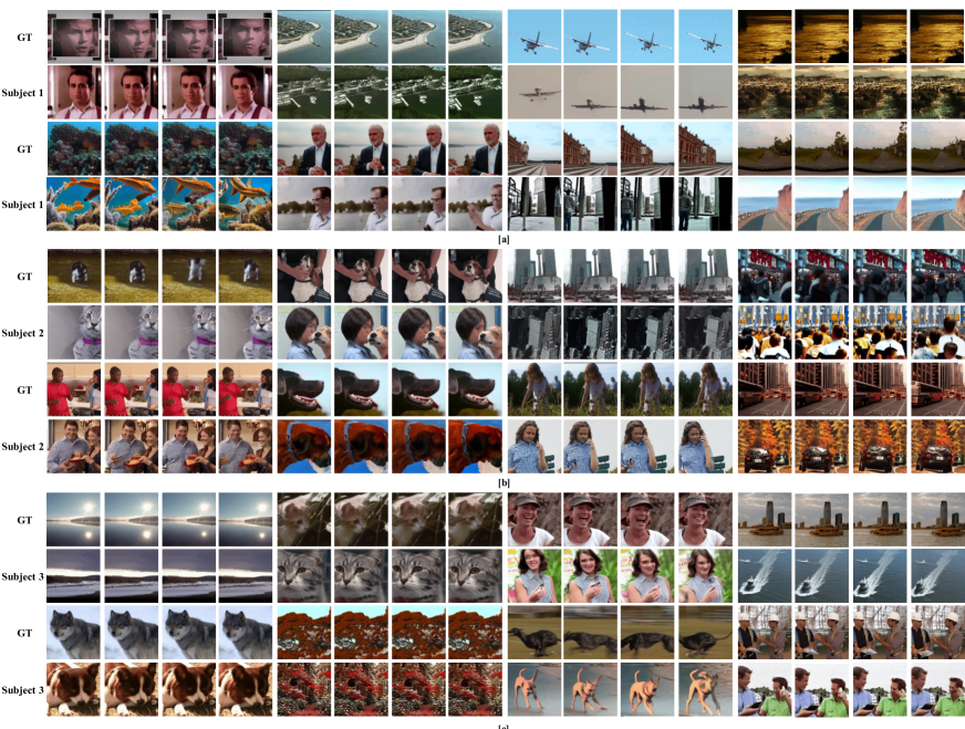
Figure 7: Videos generated by our models: [a] Decoding outcomes for Subject 1, [b] Decoding outcomes for Subject 2, [c] Decoding outcomes for Subject 3.

References

- Abraham et al. (2014) Abraham, A., Pedregosa, F., Eickenberg, M., Gervais, P., Mueller, A., Kossaifi, J., Gramfort, A., Thirion, B., and Varoquaux, G. Machine learning for neuroimaging with scikit-learn. Frontiers in neuroinformatics, 8:14, 2014.
- Bao et al. (2022) Bao, F., Li, C., Zhu, J., and Zhang, B. Analytic-dpm: an analytic estimate of the optimal reverse variance in diffusion probabilistic models. arXiv preprint arXiv:2201.06503, 2022.
- Bartels et al. (2008) Bartels, A., Zeki, S., and Logothetis, N. K. Natural vision reveals regional specialization to local motion and to contrast-invariant, global flow in the human brain. Cerebral cortex, 18(3):705–717, 2008.
- Beliy et al. (2019) Beliy, R., Gaziv, G., Hoogi, A., Strappini, F., Golan, T., and Irani, M. From voxels to pixels and back: Self-supervision in natural-image reconstruction from fmri. ArXiv, abs/1907.02431, 2019.
- Buxton (2009) Buxton, R. B. Introduction to functional magnetic resonance imaging: principles and techniques. Cambridge university press, 2009.
- Chen et al. (2020) Chen, N., Zhang, Y., Zen, H., Weiss, R. J., Norouzi, M., and Chan, W. Wavegrad: Estimating gradients for waveform generation. arXiv preprint arXiv:2009.00713, 2020.
- Chen et al. (2022) Chen, Z., Qing, J., Xiang, T., Yue, W. L., and Zhou, J. H. Seeing beyond the brain: Masked modeling conditioned diffusion model for human vision decoding. In arXiv, November 2022. URL https://arxiv.org/abs/2211.06956.
- Chen et al. (2023) Chen, Z., Qing, J., and Zhou, J. H. Cinematic mindscapes: High-quality video reconstruction from brain activity. arXiv preprint arXiv:2305.11675, 2023.
- de Zwart et al. (2009) de Zwart, J. A., van Gelderen, P., Jansma, J. M., Fukunaga, M., Bianciardi, M., and Duyn, J. H. Hemodynamic nonlinearities affect bold fmri response timing and amplitude. Neuroimage, 47(4):1649–1658, 2009.
- Fang et al. (2021) Fang, T., Qi, Y., and Pan, G. Reconstructing perceptive images from brain activity by shape-semantic gan. ArXiv, abs/2101.12083, 2021.
- Ge et al. (2023) Ge, S., Nah, S., Liu, G., Poon, T., Tao, A., Catanzaro, B., Jacobs, D., Huang, J.-B., Liu, M.-Y., and Balaji, Y. Preserve your own correlation: A noise prior for video diffusion models. In Proceedings of the IEEE/CVF International Conference on Computer Vision, pp. 22930–22941, 2023.
- Glover (2011) Glover, G. H. Overview of functional magnetic resonance imaging. Neurosurgery Clinics, 22(2):133–139, 2011.
- He et al. (2022) He, Y., Yang, T., Zhang, Y., Shan, Y., and Chen, Q. Latent video diffusion models for high-fidelity video generation with arbitrary lengths. arXiv preprint arXiv:2211.13221, 2022.
- Hénaff et al. (2021) Hénaff, O. J., Bai, Y., Charlton, J. A., Nauhaus, I., Simoncelli, E. P., and Goris, R. L. Primary visual cortex straightens natural video trajectories. Nature communications, 12(1):5982, 2021.
- Ho et al. (2020) Ho, J., Jain, A., and Abbeel, P. Denoising diffusion probabilistic models. Advances in Neural Information Processing Systems, 33:6840–6851, 2020.
- Ho et al. (2022a) Ho, J., Chan, W., Saharia, C., Whang, J., Gao, R., Gritsenko, A., Kingma, D. P., Poole, B., Norouzi, M., Fleet, D. J., et al. Imagen video: High definition video generation with diffusion models. arXiv preprint arXiv:2210.02303, 2022a.
- Ho et al. (2022b) Ho, J., Salimans, T., Gritsenko, A., Chan, W., Norouzi, M., and Fleet, D. J. Video diffusion models, 2022b.
- Kay et al. (2017) Kay, W., Carreira, J., Simonyan, K., Zhang, B., Hillier, C., Vijayanarasimhan, S., Viola, F., Green, T., Back, T., Natsev, P., et al. The kinetics human action video dataset. arXiv preprint arXiv:1705.06950, 2017.
- Kingma & Welling (2013) Kingma, D. P. and Welling, M. Auto-encoding variational bayes. arXiv preprint arXiv:1312.6114, 2013.
- Kupershmidt et al. (2022) Kupershmidt, G., Beliy, R., Gaziv, G., and Irani, M. A penny for your (visual) thoughts: Self-supervised reconstruction of natural movies from brain activity. arXiv preprint arXiv:2206.03544, 2022.
- Li et al. (2022) Li, J., Li, D., Xiong, C., and Hoi, S. Blip: Bootstrapping language-image pre-training for unified vision-language understanding and generation. In International Conference on Machine Learning, pp. 12888–12900. PMLR, 2022.
- Li et al. (2024) Li, M., Qu, T., Yao, R., Sun, W., and Moens, M.-F. Alleviating exposure bias in diffusion models through sampling with shifted time steps. International Conference on Learning Representations, 2024.
- Lin et al. (2022) Lin, S., Sprague, T., and Singh, A. K. Mind reader: Reconstructing complex images from brain activities. arXiv preprint arXiv:2210.01769, 2022.
- Liu et al. (2022) Liu, L., Ren, Y., Lin, Z., and Zhao, Z. Pseudo numerical methods for diffusion models on manifolds. arXiv preprint arXiv:2202.09778, 2022.
- Lu et al. (2022a) Lu, C., Zhou, Y., Bao, F., Chen, J., Li, C., and Zhu, J. Dpm-solver: A fast ode solver for diffusion probabilistic model sampling in around 10 steps. Advances in Neural Information Processing Systems, 35:5775–5787, 2022a.
- Lu et al. (2022b) Lu, C., Zhou, Y., Bao, F., Chen, J., Li, C., and Zhu, J. Dpm-solver++: Fast solver for guided sampling of diffusion probabilistic models. arXiv preprint arXiv:2211.01095, 2022b.
- Mozafari et al. (2020) Mozafari, M., Reddy, L., and van Rullen, R. Reconstructing natural scenes from fmri patterns using bigbigan. 2020 International Joint Conference on Neural Networks (IJCNN), pp. 1–8, 2020.
- Nichol & Dhariwal (2021) Nichol, A. Q. and Dhariwal, P. Improved denoising diffusion probabilistic models. In International Conference on Machine Learning, pp. 8162–8171. PMLR, 2021.
- Ning et al. (2023) Ning, M., Sangineto, E., Porrello, A., Calderara, S., and Cucchiara, R. Input perturbation reduces exposure bias in diffusion models. arXiv preprint arXiv:2301.11706, 2023.
- Ning et al. (2024) Ning, M., Li, M., Su, J., Salah, A. A., and Ertugrul, I. O. Elucidating the exposure bias in diffusion models. International Conference on Learning Representations, 2024.
- Nishimoto et al. (2011) Nishimoto, S., Vu, A. T., Naselaris, T., Benjamini, Y., Yu, B., and Gallant, J. L. Reconstructing visual experiences from brain activity evoked by natural movies. Current biology, 21(19):1641–1646, 2011.
- Parrish et al. (2000) Parrish, T. B., Gitelman, D. R., LaBar, K. S., and Mesulam, M.-M. Impact of signal-to-noise on functional mri. Magnetic Resonance in Medicine: An Official Journal of the International Society for Magnetic Resonance in Medicine, 44(6):925–932, 2000.
- Poole et al. (2022) Poole, B., Jain, A., Barron, J. T., and Mildenhall, B. Dreamfusion: Text-to-3d using 2d diffusion. arXiv preprint arXiv:2209.14988, 2022.
- Qian et al. (2023) Qian, X., Wang, Y., Fu, Y., Xue, X., and Feng, J. Semantic neural decoding via cross-modal generation. arXiv preprint arXiv:2303.14730, 2023.
- Radford et al. (2021) Radford, A., Kim, J. W., Hallacy, C., Ramesh, A., Goh, G., Agarwal, S., Sastry, G., Askell, A., Mishkin, P., Clark, J., et al. Learning transferable visual models from natural language supervision. In International conference on machine learning, pp. 8748–8763. PMLR, 2021.
- Rombach et al. (2022) Rombach, R., Blattmann, A., Lorenz, D., Esser, P., and Ommer, B. High-resolution image synthesis with latent diffusion models. In Proceedings of the IEEE/CVF Conference on Computer Vision and Pattern Recognition, pp. 10684–10695, 2022.
- Seeliger et al. (2017) Seeliger, K., Güçlü, U., Ambrogioni, L., Güçlütürk, Y., and van Gerven, M. Generative adversarial networks for reconstructing natural images from brain activity. NeuroImage, 181:775–785, 2017.
- Shen et al. (2019) Shen, G., Dwivedi, K., Majima, K., Horikawa, T., and Kamitani, Y. End-to-end deep image reconstruction from human brain activity. Frontiers in computational neuroscience, 13:21, 2019.
- Singer et al. (2022) Singer, U., Polyak, A., Hayes, T., Yin, X., An, J., Zhang, S., Hu, Q., Yang, H., Ashual, O., Gafni, O., et al. Make-a-video: Text-to-video generation without text-video data. arXiv preprint arXiv:2209.14792, 2022.
- Sohl-Dickstein et al. (2015) Sohl-Dickstein, J., Weiss, E., Maheswaranathan, N., and Ganguli, S. Deep unsupervised learning using nonequilibrium thermodynamics. In International Conference on Machine Learning, pp. 2256–2265. PMLR, 2015.
- Song et al. (2020) Song, J., Meng, C., and Ermon, S. Denoising diffusion implicit models. arXiv:2010.02502, October 2020. URL https://arxiv.org/abs/2010.02502.
- Sun et al. (2023a) Sun, J., Li, M., and Moens, M.-F. Decoding realistic images from brain activity with contrastive self-supervision and latent diffusion. In Proceedings of the 26th European Conference on Artificial Intelligence (ECAI 2023), 2023, 2023a.
- Sun et al. (2023b) Sun, J., Li, M., Zhang, Y., Moens, M.-F., Chen, Z., and Wang, S. Contrast, attend and diffuse to decode high-resolution images from brain activities. In Thirty-seventh Conference on Neural Information Processing Systems, 2023b. URL https://openreview.net/forum?id=YZSLDEE0mw.
- Tong et al. (2022) Tong, Z., Song, Y., Wang, J., and Wang, L. Videomae: Masked autoencoders are data-efficient learners for self-supervised video pre-training. Advances in neural information processing systems, 35:10078–10093, 2022.
- Uğurbil et al. (2013) Uğurbil, K., Xu, J., Auerbach, E. J., Moeller, S., Vu, A. T., Duarte-Carvajalino, J. M., Lenglet, C., Wu, X., Schmitter, S., Van de Moortele, P. F., et al. Pushing spatial and temporal resolution for functional and diffusion mri in the human connectome project. Neuroimage, 80:80–104, 2013.
- Van Essen et al. (2013) Van Essen, D. C., Smith, S. M., Barch, D. M., Behrens, T. E., Yacoub, E., Ugurbil, K., Consortium, W.-M. H., et al. The wu-minn human connectome project: an overview. Neuroimage, 80:62–79, 2013.
- Varela et al. (2017) Varela, F. J., Thompson, E., and Rosch, E. The embodied mind, revised edition: Cognitive science and human experience. MIT press, 2017.
- Vetter et al. (2014) Vetter, P., Smith, F. W., and Muckli, L. Decoding sound and imagery content in early visual cortex. Current Biology, 24(11):1256–1262, 2014.
- Wang et al. (2022) Wang, C., Yan, H., Huang, W., Li, J., Wang, Y., Fan, Y.-S., Sheng, W., Liu, T., Li, R., and Chen, H. Reconstructing rapid natural vision with fmri-conditional video generative adversarial network. Cerebral Cortex, 32(20):4502–4511, 2022.
- Wang et al. (2004) Wang, Z., Bovik, A. C., Sheikh, H. R., and Simoncelli, E. P. Image quality assessment: from error visibility to structural similarity. IEEE transactions on image processing, 13(4):600–612, 2004.
- Wen et al. (2018) Wen, H., Shi, J., Zhang, Y., Lu, K.-H., Cao, J., and Liu, Z. Neural encoding and decoding with deep learning for dynamic natural vision. Cerebral cortex, 28(12):4136–4160, 2018.
- Wu et al. (2023) Wu, J. Z., Ge, Y., Wang, X., Lei, S. W., Gu, Y., Shi, Y., Hsu, W., Shan, Y., Qie, X., and Shou, M. Z. Tune-a-video: One-shot tuning of image diffusion models for text-to-video generation. In Proceedings of the IEEE/CVF International Conference on Computer Vision, pp. 7623–7633, 2023.
- Zhou et al. (2013) Zhou, D., Rangan, A. V., McLaughlin, D. W., and Cai, D. Spatiotemporal dynamics of neuronal population response in the primary visual cortex. Proceedings of the National Academy of Sciences, 110(23):9517–9522, 2013.
- Zhou et al. (2022) Zhou, D., Wang, W., Yan, H., Lv, W., Zhu, Y., and Feng, J. Magicvideo: Efficient video generation with latent diffusion models. arXiv preprint arXiv:2211.11018, 2022.