Universitat de València
E-46100 Burjassot, Spain
33email: antonio.baeza@uv.es, mulet@uv.es 44institutetext: R. Bürger 55institutetext: CI2MA & Departamento de Ingeniería Matemática
Universidad de Concepción
Casilla 160-C, Concepción, Chile
55email: rburger@ing-mat.udec.cl 66institutetext: D. Zorío (Corresponding author) 77institutetext: CI2MA, Universidad de Concepción
Casilla 160-C, Concepción, Chile
77email: dzorio@ci2ma.udec.cl
This version of the article has been accepted for publication, after a peer-review process, and is subject to Springer Nature’s AM terms of use, but is not the Version of Record and does not reflect post-acceptance improvements, or any corrections. The Version of Record is available online at:
On the efficient computation of smoothness indicators for a class of WENO reconstructions
Abstract
Common smoothness indicators used in Weighted Essentially Non-Oscillatory (WENO) reconstructions [Jiang, G.S., Shu, C.W.: Efficient implementation of Weighted ENO schemes, J. Comput. Phys. 126, 202–228 (1996)] have quadratic cost with respect to the order. A set of novel smoothness indicators with linear cost of computation with respect to the order is presented. These smoothness indicators can be used in the context of schemes of the type introduced by Yamaleev and Carpenter [Yamaleev, N.K., Carpenter, M.H.: A systematic methodology to for constructing high-order energy stable WENO schemes. J. Comput. Phys. 228(11), 4248–4272 (2009)]. The accuracy properties of the resulting non-linear weights are the same as those arising from using the traditional Jiang-Shu smoothness indicators in Yamaleev-Carpenter-type reconstructions. The increase of the efficiency and ease of implementation are shown.
Keywords:
finite-difference schemes, WENO reconstructions, smoothness indicators1 Introduction
1.1 Scope
Weighted Essentially Non-Oscillatory (WENO) schemes are a very useful and powerful tool to reconstruct functions from discrete data. They avoid an oscillatory behaviour in presence of a discontinuity and attain the optimal interpolation order whenever possible when the data is smooth. The most common contexts in which these schemes are used are finite-difference or finite-volume schemes discretizing hyperbolic conservation laws, whose solutions are typically non-smooth (weak solutions) and usually present strong shocks. WENO reconstructions are building blocks of numerical schemes that properly handle discontinuous solutions, and represent a popular way to construct high-order methods. However, it is well known that despite the recognized efficiency of these schemes, the most expensive part of the algorithm is the computation of local smoothness indicators, whose computational cost is quadratic with respect to the order of the scheme.
It is the purpose of this work to advance a novel design of smoothness indicators so that they are cheaper to compute (namely, at linear cost in terms of the order of accuracy) than the Jiang-Shu smoothness indicators JiangShu96 in the context of Yamaleev-Carpenter reconstructions YamaleevCarpenter2009 , while both properties of optimal accuracy in case of smoothness and robust capture of discontinuities are ensured. To do so, we first advance theoretical considerations that are needed for their foundation, and that allow us to ultimately define the new smoothness indicators along with the associated weight design. The resulting WENO schemes are addressed as “Fast WENO” (FWENO) schemes.
1.2 Related work
The classical WENO schemes were proposed by Jiang and Shu JiangShu96 ; shu98 as an improvement of the original proposal of Liu et al. LiuOsherChan94 . The idea is to build a weighted combination of interpolators, with the weights depending on smoothness indicators that tune the weight according to the data. The smoothness indicators defined by Jiang and Shu are designed in a way such that they take small values if the data used to construct the indicator is smooth and large values otherwise, with the additional property that the values of indicators constructed with smooth data are close to each other. This property is important as the order of accuracy of the final reconstruction is strongly dependent on it.
Several years later, Yamaleev and Carpenter YamaleevCarpenter2009O3 proposed a new third-order WENO scheme, which was later on extended to arbitrary order in YamaleevCarpenter2009 (henceforth, YC-WENO scheme). In this case, the non-linear weights are based instead on a ratio between a high-order undivided difference, which is very small when the data is smooth and large if a discontinuity crosses the data stencil, and the original Jiang-Shu smoothness indicators. In this latter case the accuracy of the scheme is based on the asymptotic convergence of the undivided difference and the smoothness indicators, rather than the closeness between the latter ones. This allows one to simplify the smoothness indicators, which is presented in this paper.
1.3 Outline of this paper
The remainder of the paper is organized as follows. In Section 2, we provide the theoretical background for the novel smoothness indicators. Section 3 is devoted to the definition of the smoothness indicators, the construction of the corresponding numerical scheme and the analysis of its accuracy. Section 4 contains several numerical experiments in which the new algorithm is compared against the previous ones in terms of accuracy and efficiency. Finally, in Section 5 some conclusions are drawn.
2 Preliminaries
2.1 Asymptotic properties of functions
We recall that for ,
and define the more restrictive property
For positive functions and , the properties
imply that for , and . Here and in what follows it is always understood that expressions of the form , correspond to . Similarly, taking into account that for , where we define , it follows that for a positive function ,
therefore, if is positive, then implies .
2.2 Point values and cell averages of smooth functions
Finite-difference and finite-volume schemes for hyperbolic conservation laws are based on discretizations of the solution by means of point values and cell averages, respectively. The following lemmas state the same result for both cases so that we can analyze them in a unified way.
Lemma 1
Assume that a function satisfies for and . Then .
Proof
The -th order Taylor expansion of yields
which implies that
which in turn means that .
Lemma 2
Let . Assume that
Then
| (2.1) | ||||
| (2.2) |
where
Proof
Our purpose is to apply Lemma 1 to the difference
to obtain (2.1) and alternatively, to the expression
| (2.3) |
to obtain (2.2). For (2.1), it follows directly that
Since there clearly holds that if and only if is even and .
For (2.2), we obtain from (2.3) multiplied by
and for ,
On the other hand, the Leibniz formula for higher derivatives yields
Therefore, for we get , where
Since
we obtain
| (2.4) |
Now, if , then if is even and
if is odd, since the sign of all summands is the sign of . On the other hand, if , since , then , so all summands in (2.4) have the same sign, which yields for any . Therefore if and only if is odd and . In both cases it follows from the definition of and in the assumptions that
so Lemma 1 yields the final result.
3 Modified smoothness indicators and new weight design
In this section the modified WENO schemes with the new smoothness indicators are considered for YC-WENO-type schemes YamaleevCarpenter2009 . Schemes of order are based on a stencil
| (3.1) |
where results either from a point-value or a cell-average discretization of a function :
for constant , where we wish to reconstruct at . In the following sections we introduce the “Fast WENO” (FWENO) schemes.
3.1 Fast WENO (FWENO) schemes of order ,
The traditional Jiang-Shu smoothness indicators JiangShu96 are defined by
| (3.2) |
where are the corresponding interpolating polynomials associated to the substencils , . These smoothness indicators have been typically used in the literature involving WENO schemes, although their evaluation is computationally expensive (quadratic with respect to the order, as becomes evident from the identity deduced from (SINUM2011, , Proposition 5) (see subsection 3.3 for a more efficient computation, but still quadratic in ):
We propose new smoothness indicators for both (point-value and cell-average) reconstructions that have linear cost with respect to the order (namely, they involve additions and multiplications), and that are defined by
| (3.3) |
A detailed analysis on the computational cost of the smoothness indicators in both cases is included in Section 3.3. The remaining parts of the algorithm are the same as those defined in YamaleevCarpenter2009 for the YC-WENO schemes. For the sake of exposition, we briefly describe it:
Input: , with , and .
-
1.
Compute interpolating polynomials
where computes approximate point values from either point values or cell averages, according to the discretization.
-
2.
Compute the new smoothness indicators (3.3).
-
3.
Obtain the corresponding squared undivided differences of order :
(3.4) -
4.
Compute the terms
(3.5) where are the ideal linear weights, for some chosen by the user such that and .
-
5.
Generate the WENO weights:
(3.6) -
6.
Obtain the reconstruction at :
(3.7)
Output: .
Remark 1
As stated above, the difference between our proposed WENO method and YC-WENO is the usage of the new smoothness indicators as defined in (3.3) in the former case and the usage of the classical smoothness indicators as defined in (3.2) in the latter case. In turn, the difference between JS-WENO and YC-WENO schemes is that in the former case the coefficients are defined by
| (3.8) |
instead of (3.5).
3.2 Accuracy properties of FWENO schemes
We next analyze the accuracy properties of the novel smoothness indicators.
Lemma 3
Let , and a grid be defined by for . Assume that given by (3.1) is a stencil such that , with for and , , , and assume that there exists such that . Furthermore, assume that the quantities are given by (3.3). Then .
On the other hand, if and has a unique discontinuity located in , then there exist indices with such that and .
Proof
If , then by Lemma 2 there holds
Therefore, in particular, one has
Let us now assume that for some , . Then, again by Lemma 2:
Thus, we have the following: If , then
Otherwise, that is if , we get
since clearly by definition .
Finally, if has a unique discontinuity at , then there exists such that , whereas for . Hence, if we select for instance and if , or and if , then clearly and .
Remark 2
The case for the FWENO method is the same as in the original YC-WENO method, since in this case the proposed smoothness indicators are the same. In this case, the statement of Lemma 3 does not hold in general, since one can have if .
Theorem 3.1
Under the same conditions and notation as in Lemma 3, with and dropping the role of , there holds
Proof
We first assume smoothness with a critical point of order . Then, by Lemma 3, the new smoothness indicators satisfy . We consider in first place the case . Then there holds for :
Hence, the non-linear weights satisfy
On the other hand, with . Therefore, denoting by
the value at of the optimal -th order polynomial, we have
Taking into account that , we have
We next analyze the exponent of the left summand, splitting the discussion into two cases. On one hand, if , then and there holds
where the last inequality holds since by assumption .
On the other hand, if , then and then, since by assumption ,
Thus, for the case there holds .
In second place, we assume now , then, using that , there holds
Finally, if a discontinuity crosses the data, assume that is the set of indices associated to the substencils , , in which the discontinuity is not crossed ( by the second part of Lemma 3), and the set of the remaining whose corresponding substencils , , are crossed by the discontinuity. Then if ,
and if ,
Therefore, if ,
and if ,
Thus, we conclude that
Now using that and , we have
Therefore , which completes the proof.
Remark 3
According to this result, the only case in which our method loses accuracy with respect to the reconstruction with ideal linear weights is when , in which the accuracy order decays to , namely, one unit less than the optimal accuracy order, .
3.3 Efficiency properties of FWENO schemes
We conclude this section with a comparison involving the number of operations of an FWENO interpolator with respect to the traditional JS-WENO and YC-WENO interpolators. In order to do so, we invoke (SINUM2011, , Propositions 1 and 5) to conclude that the evaluation of the reconstruction polynomials at the reconstruction point and the classical Jiang-Shu smoothness indicators can be respectively written as
where are constants with respect to the data from the stencil.
This expression can be further simplified by taking into account that is a positive semi-definite quadratic form defined on with rank , therefore it can be expressed in a more convenient and numerically stable manner as a sum of squares of linear combinations of . Specifically, for each , let be the matrix associated to , i.e.
The matrix is semi-positively-definite with rank and therefore admits a decomposition as , where is a permutation matrix associated to the permutation of , is lower triangular with unit entries in the diagonal and , with , . This yields the following simplified expression:
The cost associated to each reconstruction of lower order is thus additions and multiplications, while the cost associated to each classical smoothness indicators is additions and multiplications. Hence, the cost associated to the computation of the whole set of reconstructions of lower order is additions and multiplications, whereas the cost associated to the computation of the whole set of classical smoothness indicators is additions and multiplications.
Now let us analyze the cost associated with the FWENO smoothness indicators (3.3). In this case, we also can reduce the number of operations by taking into consideration that the novel smoothness indicators satisfy a simple recurrence relation, in a way that their computation can be simplified in the following algorithm, involving a linear cost both in terms of additions and in terms of multiplications:
-
1.
Compute
Operations: additions and multiplications.
-
2.
Compute
Operations: additions.
-
3.
Compute
Operations: additions.
Therefore, the cost associated to the whole set of smoothness indicators involves additions and multiplications.
Now, YC-WENO and FWENO schemes also involve the computation of (3.4), which involves additions and multiplications.
As for the terms , we have two cases: for JS-WENO schemes, the expression for them is (3.8), and therefore the number of operations for each one is one addition, multiplications and one division; therefore, the total cost for all them is additions, multiplications and divisions. As for YC-WENO and FWENO schemes, the expression to be computed is (3.5), and the number of operations associated to each one of them is two additions, multiplications and one division, being thus the total cost additions, multiplications and divisions.
The non-linear weights have the same expression (3.6) in all cases. The denominator is the same for all the weights, and therefore one can previously store the value of and then compute , converting thus divisions, much more expensive than multiplications, in to one division and multiplications. Therefore, the total cost corresponds now to additions and one division associated with the computation of and multiplications (one multiplication per weight). Finally, the reconstruction expression (3.7) is also common in the three schemes, and corresponds to additions and multiplications.
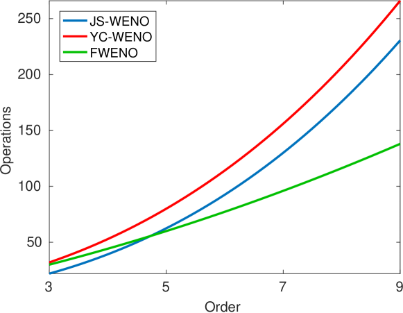
The number of operations associated to each term and the grand total of operations for each method is summarized in Tables 1 to 3, where it can be drawn as a conclusion that the number of operations of JS-WENO and YC-WENO is cubic with respect to the order, whereas the number of operations associated to FWENO increases quadratically with respect to the order. Therefore, the complexity of the smoothness indicators is indeed a crucial factor in terms of the impact on the computational cost, and using simplified alternatives can indeed reduce significantly the overall computational cost of the WENO interpolator.
| Order | JS-WENO | ||
| Operations | Additions | Multiplications | Divisions |
| SUM | |||
| TOTAL | |||
| Order | YC-WENO | ||
| Operations | Additions | Multiplications | Divisions |
| SUM | |||
| TOTAL | |||
| Order | FWENO | ||
| Operations | Additions | Multiplications | Divisions |
| SUM | |||
| TOTAL | |||
A graphical comparison between the cost associated to each scheme is also shown in Figure 1, with , and .
4 Numerical experiments
We now present some numerical experiments for schemes based on finite differences, as introduced in ShuOsher89 ; ShuOsher1989 , combined with high-order WENO reconstructions to discretize hyperbolic conservation laws. Results obtained by the new FWENO scheme are compared with those generated by the JS-WENO and YC-WENO schemes. The exponent for JS-WENO method is chosen as , while the exponents and for both YC-WENO and FWENO methods are chosen as and . Finally, we set in all the numerical experiments , so that this parameter has the sole role of avoiding divisions by zero.
4.1 1D conservation law experiments
Example 1: Linear advection equation
| YC-WENO5 | FWENO5 | |||||||
|---|---|---|---|---|---|---|---|---|
| Err. | Err. | Err. | Err. | |||||
| 10 | 1.02e-03 | — | 1.55e-03 | — | 1.01e-03 | — | 1.66e-03 | — |
| 20 | 3.27e-05 | 4.96 | 5.16e-05 | 4.91 | 3.27e-05 | 4.95 | 5.16e-05 | 5.01 |
| 40 | 1.01e-06 | 5.01 | 1.60e-06 | 5.01 | 1.01e-06 | 5.01 | 1.60e-06 | 5.01 |
| 80 | 3.15e-08 | 5.01 | 4.94e-08 | 5.01 | 3.15e-08 | 5.01 | 4.94e-08 | 5.01 |
| 160 | 9.79e-10 | 5.01 | 1.54e-09 | 5.01 | 9.79e-10 | 5.01 | 1.54e-09 | 5.01 |
| 320 | 3.05e-11 | 5.00 | 4.79e-11 | 5.00 | 3.05e-11 | 5.00 | 4.79e-11 | 5.00 |
| 640 | 9.52e-13 | 5.00 | 1.50e-12 | 5.00 | 9.53e-13 | 5.00 | 1.50e-12 | 5.00 |
We first apply the fifth-order accurate YC-WENO5 and FWENO schemes to the initial-boundary value problem for the linear advection equation
which has the solution . We run several simulations with final time and grid spacings and measure the resulting errors both in the and norms. From the numerical results, which are shown in Table 4, one can conclude that both schemes converge numerically at approximate fifth-order rate, which is consistent with our theoretical analysis. In fact, the results for the YC-WENO and FWENO schemes are nearly identical.
Example 2: Burgers equation
| YC-WENO5 | FWENO5 | |||||||
|---|---|---|---|---|---|---|---|---|
| Err. | Err. | Err. | Err. | |||||
| 40 | 2.44e-05 | 4.95 | 2.52e-04 | 4.70 | 2.73e-05 | 5.11 | 2.50e-04 | 4.69 |
| 80 | 7.89e-07 | 5.08 | 9.70e-06 | 5.05 | 7.89e-07 | 5.08 | 9.70e-06 | 5.05 |
| 160 | 2.32e-08 | 5.05 | 2.94e-07 | 5.03 | 2.32e-08 | 5.05 | 2.94e-07 | 5.03 |
| 320 | 7.01e-10 | 5.04 | 8.96e-09 | 5.03 | 7.01e-10 | 5.04 | 8.96e-09 | 5.03 |
| 640 | 2.14e-11 | 5.02 | 2.73e-10 | 5.02 | 2.14e-11 | 5.02 | 2.73e-10 | 5.02 |
| 1280 | 6.59e-13 | 5.02 | 8.41e-12 | 5.00 | 6.59e-13 | 5.02 | 8.41e-12 | 5.00 |
 |
|
 |
 |
We now solve numerically the following initial-boundary value problem for the inviscid Burgers equation:
A first simulation is run until , in which the solution remains smooth. We compare both YC-WENO and FWENO schemes in the results shown in Table 5, where it can be observed that both methods attain again fifth order accuracy, producing an almost identical error.
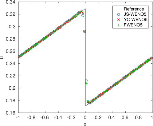
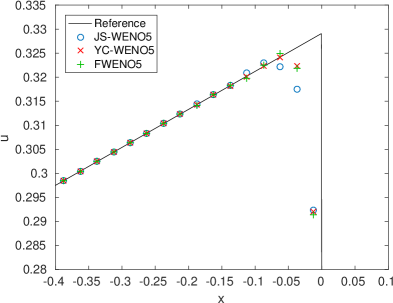
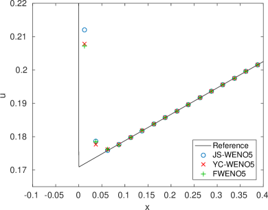
The simulation is now run until . At , the wave breaks and a shock is generated. Therefore, we use the Donat-Marquina flux-splitting algorithm DonatMarquina96 . The results shown in Figure 2 correspond to the fifth-order schemes, with a resolution of cells, and are compared with a reference solution computed with cells. The results obtained for all three methods are very similar, and therefore one can conclude that in this case using the new smoothness indicators does not appreciably affect the quality of the solution.
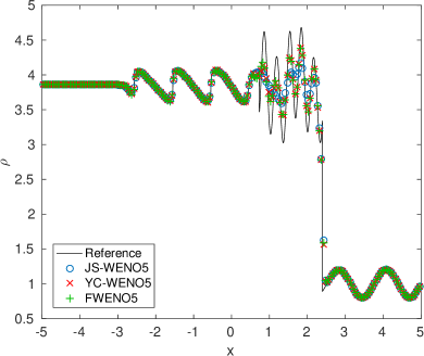
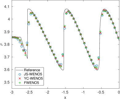
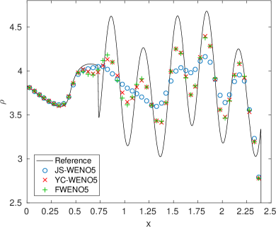
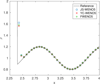
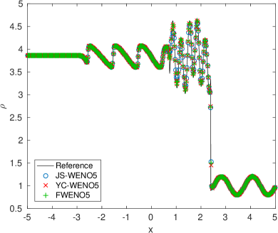
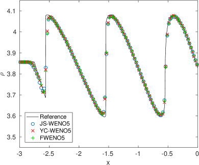
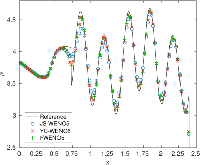
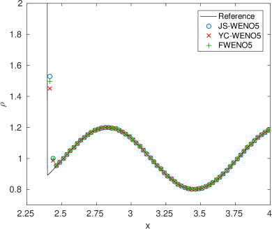
Example 3: Shu-Osher problem, 1D Euler equations of gas dynamics
 |
 |
 |
 |
 |
 |
 |
 |
 |
 |
 |
The 1D Euler equations for gas dynamics are given by and , where is the density, is the velocity and is the specific energy of the system. The variable stands for the pressure and is given by the equation of state
where is the adiabatic constant that will be taken as . The spatial domain is , and the initial condition
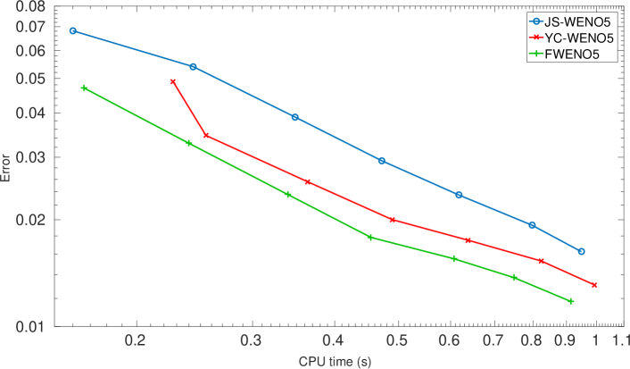
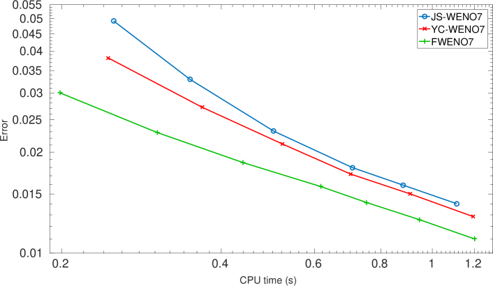
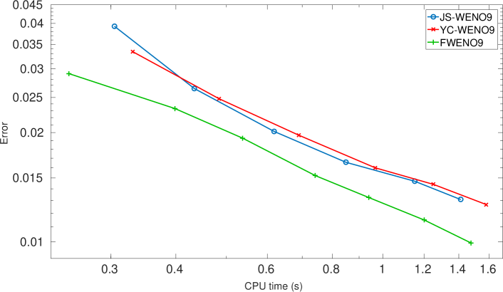
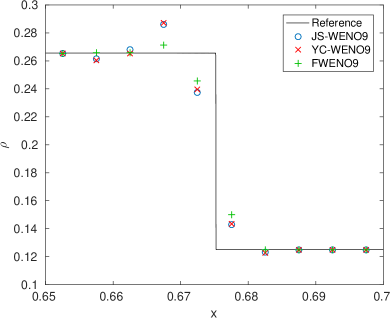
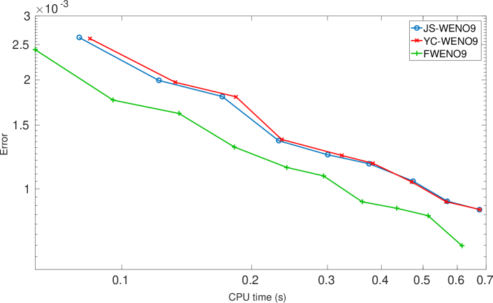
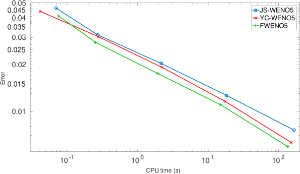
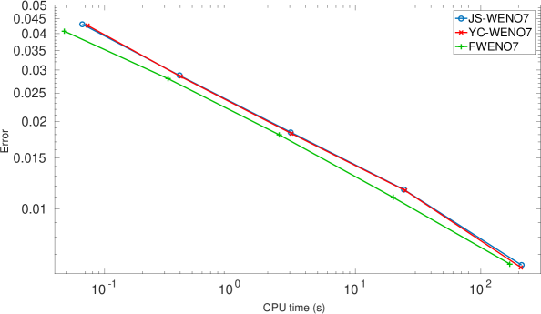
stipulates the interaction of a Mach 3 shock with a sine wave and is complemented with left inflow and right outflow boundary conditions. We run the simulation until and compare the schemes against a reference solution computed with a resolution of . Figures 3 and 4 display the results obtained by fifth-order schemes with resolutions of and cells, respectively. The results are similar for the YC-WENO and FWENO schemes and are slightly less sharply resolved for the JS-WENO scheme. In order to highlight the superior performance of the FWENO scheme, we also plot the numerical error against the CPU time for schemes of order , with , which is shown in Figures 5–7. These results clearly indicate that the scheme with the new smoothness indicators is more efficient (in terms of error reduction versus CPU time) than the schemes that employ the traditional Jiang-Shu smoothness indicators.
Example 4 (Sod shock tube problem, 1D Euler equations of gas dynamics)
 |
 |
 |
 |
 |
We now apply WENO schemes to the 1D Euler equations of gas dynamics on with the initial condition
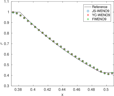
and left and right Dirichlet boundary conditions corresponding to the shock tube problem proposed by Sod Sod1978 . This problem has been tackled in many other papers afterwards, such as in BurgerKumarZorio2017 . The numerical result is produced by ninth-order schemes with a resolution of cells compared against a reference solution which has been computed with a resolution of by the classical JS-WENO scheme. The simulation is run until and the results are depicted in Figure 8. It turns our that the schemes produce very similar results. In fact, the most remarkable differences are favorable to our proposed FWENO scheme, since the behavior is slightly less oscillatory near the contact discontinuity and the shock. Finally, an efficiency comparison is presented in Figure 9, where it can be concluded that our FWENO scheme turns out to be again more efficient than their classical JS-WENO and YC-WENO counterparts.
4.2 2D conservation law experiments
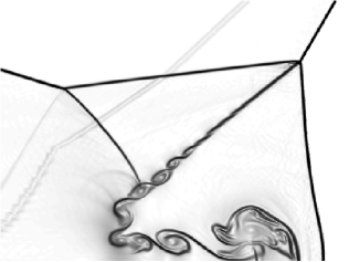
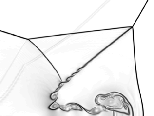
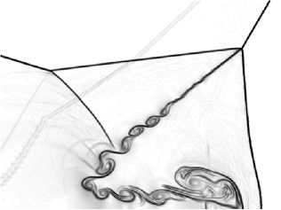
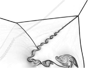
Example 5 (double Mach reflection, 2D Euler equations of gas dynamics)
 |
 |
| (a) JS-WENO5, | (b) YC-WENO5, |
 |
 |
| (c) FWENO5, | (d) JS-WENO5, |
 |
 |
| (e) YC-WENO5, | (f) FWENO5, |
The two-dimensional Euler equations for inviscid gas dynamics are given by
with
Here is the density, is the velocity, is the specific energy, and is the pressure that is given by the equation of state
where the adiabatic constant is again chosen as . This experiment uses these equations to model a vertical right-going Mach 10 shock colliding with an equilateral triangle. By symmetry, this is equivalent to a collision with a ramp with a slope of with respect to the horizontal line.
For sake of simplicity, we consider the equivalent problem in a rectangle, consisting in a rotated shock, whose vertical angle is . The domain is the rectangle , whose initial conditions are
We impose inflow boundary conditions, with value , at the left side, , outflow boundary conditions both at and , reflecting boundary conditions at and inflow boundary conditions at the upper side, , which mimics the shock at its actual traveling speed:
We run different simulations until both at a resolution of points and a resolution of points, shown in Figure 10, in both cases with and involving the JS-WENO scheme, the YC-WENO method and our FWENO scheme for the case of fifth-order accuracy. The results show that both YC-WENO and FWENO schemes produce sharper resolution than JS-WENO, and in turn they have similar resolution between then.
Example 6: Riemann problem
 |
 |
| (a) JS-WENO5, | (b) YC-WENO5, |
 |
 |
| (c) FWENO5, | (d) JS-WENO5, |
 |
 |
| (e) YC-WENO5, | (f) FWENO5, |
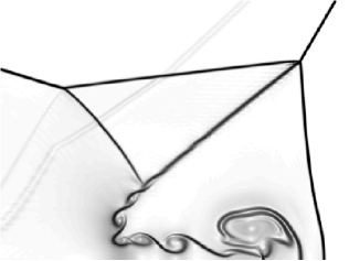
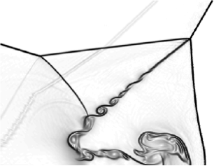
Finally, we solve numerically a Riemann problem for the 2D Euler equations on the domain . Riemann problems for 2D Euler equations were first studied in SchulzRinne . The initial data is taken from (KurganovTadmor, , Sect. 3, Config. 3):
and
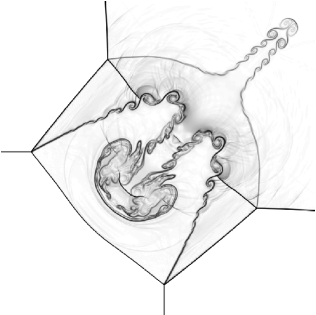
with the same equation of state as in the previous test. The simulation is performed taking , with the final time , , resolutions and and comparing the same schemes with the same parameters as in Example 5. The results are shown in Figure 11. The same conclusions as in Example 5 are drawn.
We now use the solutions computed with the grid of points as reference solutions to perform efficiency tests by comparing error versus CPU time involving numerical solutions with grid sizes , , for the corresponding fifth, seventh and ninth order schemes. The results are shown in Figure 12 and again indicate a higher performance for the FWENO scheme.
 |
 |
 |
5 Conclusions
In this paper a set of alternative smoothness indicators, cheaper than the classical Jiang-Shu ones, has been presented. The theoretical results show that when used in Yamaleev-Carpenter type weight constructions they attain the same accuracy properties than the ones obtained with the original smoothness indicators. The numerical experiments confirm all these theoretical considerations. Also, the numerical evidence obtained in the problems from hyperbolic conservation laws with weak solutions also shows that the quality of the approximation is similar in both cases, being the schemes with the modified smoothness indicators (FWENO) more efficient than their traditional counterparts (JS-WENO and YC-WENO).
As for future work, we encompass extrapolating the benefits of this new weight design with the simplified smoothness indicators in the context of WENO extrapolation for numerical boundary conditions and even generalized WENO interpolations/extrapolations in the context of non-uniform grids, in which the computational benefits of using these new smoothness indicators with respect to the traditional ones are expected to be much higher than in uniform grids.
Acknowledgements
AB, PM and DZ are supported by Spanish MINECO project MTM2017-83942-P. RB is supported by CONICYT/PIA/Concurso Apoyo a Centros Científicos y Tecnológicos de Excelencia con Financiamiento Basal AFB170001; Fondecyt project 1170473; and CRHIAM, project CONICYT/FONDAP/15130015. PM is also supported by Conicyt (Chile), project PAI-MEC, folio 80150006. DZ is also supported by Conicyt (Chile) through Fondecyt project 3170077.
References
- (1) Aràndiga, F., Baeza, A., Belda, A.M., Mulet, P.: Analysis of WENO schemes for full and global accuracy. SIAM J. Numer. Anal. 49(2), 893–915 (2011)
- (2) Bürger, R., Kenettinkara, S. K., Zorío, D.: Approximate Lax-Wendroff discontinuous Galerkin methods for hyperbolic conservation laws. Computers & Mathematics with Applications, 74(6), 1288–1310 (2017)
- (3) Donat, R., Marquina, A.: Capturing shock reflections: An improved flux formula. J. Comput. Phys. 125, 42–58 (1996)
- (4) Jiang, G.S., Shu, C.W.: Efficient implementation of Weighted ENO schemes. J. Of Comput. Phys. 126, 202–228 (1996)
- (5) Kurganov, A., Tadmor, E.: Solution of two-dimensional Riemann problems for gas dynamics without Riemann problem solvers Numer. Methods Partial Differential Equations 18, 584–608 (2002)
- (6) Liu, X-D., Osher, S., Chan, T.: Weighted essentially non-oscillatory schemes. J. Comput. Phys. 115(1) 200–212 (1994)
- (7) Schulz-Rinne, C. W.: Classification of the Riemann problem for two-dimensional gas dynamics. SIAM Journal on Mathematical Analysis 24(1), 76–88 (1993)
- (8) Shu, C.-W., Osher, S.: Efficient implementation of essentially non-oscillatory shock-capturing schemes. J. Comput. Phys. 77, 439–471 (1988)
- (9) Shu, C.-W., Osher, S.: Efficient implementation of essentially non-oscillatory shock-capturing schemes, II. J. Comput. Phys. 83(1), 32–78 (1989)
- (10) Shu, C.-W.: Essentially non-oscillatory and weighted essentially non-oscillatory schemes for hyperbolic conservation laws. In Cockburn, B., Johnson, C., Shu, C.-W. and Tadmor, E. (Quarteroni, A., Ed.): Advanced Numerical Approximation of Nonlinear Hyperbolic Equations. Lecture Notes in Mathematics, vol. 1697, Springer-Verlag, Berlin, 325–432 (1998)
- (11) Sod, G. A.: A survey of several finite difference methods for systems of nonlinear hyperbolic conservation laws. J. Comput. Phys. 27(1), 1–31 (1978)
- (12) Yamaleev, N. K., Carpenter, M. H.: Third-order Energy Stable WENO scheme. J. Comput. Phys. 228(8), 3025–3047 (2009)
- (13) Yamaleev, N. K., Carpenter, M. H.: A systematic methodology to for constructing high-order energy stable WENO schemes. J. Comput. Phys. 228(11), 4248–4272 (2009)