Eigenvalues of the magnetic Dirichlet Laplacian with constant magnetic field on discs in the strong field limit

Abstract

We consider the magnetic Dirichlet Laplacian with constant magnetic field on domains of finite measure. In the case of a disc, we prove that the eigenvalue branches with respect to the field strength behave asymptotically linear with an exponentially small remainder term as the field strength goes to infinity. We compute the asymptotic expression for this remainder term. Furthermore, we show that for sufficiently large magnetic field strengths, the spectral bound corresponding to the Pólya conjecture for the non-magnetic Dirichlet Laplacian is violated up to a sharp excess factor which is independent of the domain.

1 Introduction

In this paper, we consider the magnetic Laplacian with a constant magnetic field on an open set $\Omega\subset\mathbb{R}^{2}$ of finite Lebesgue measure. Let the vector potential $A:\mathbb{R}^{2}\rightarrow\mathbb{R}^{2}$ be given by the standard linear gauge

$$A(x_{1},x_{2})=\frac{B}{2}\begin{pmatrix}-x_{2}\\ x_{1}\end{pmatrix}$$

where the scalar $B\in\mathbb{R}$ is the strength of the constant magnetic field. The magnetic Laplacian $H_{B}^{\Omega}$ with constant magnetic field and Dirichlet boundary condition is realized by Friedrichs extension of the quadratic form

$$a[u]:=\int_{\Omega}|(-i\nabla+A)u|^{2}\,\mathrm{d}x,\qquad u\in C_{0}^{\infty}(\Omega).$$

Just as the non-magnetic Dirichlet Laplacian, the operator defined via $a[\,\cdot\,]$ is positive, self-adjoint and has compact resolvent. It admits a sequence of real, positive eigenvalues $\{\lambda_{n}(\Omega,B)\}_{n\in\mathbb{N}}$ of finite multiplicity that accumulate at infinity only. The corresponding eigenfunctions $\{\psi_{n}\}_{n\in\mathbb{N}}$ satisfy the weak eigenvalue equation

$$\int_{\Omega}(-i\nabla+A)\psi_{n}\cdot\overline{(-i\nabla+A)\varphi}\,\mathrm{d}x=\lambda_{n}(\Omega,B)\int_{\Omega}\psi_{n}\overline{\varphi}\,\mathrm{d}x,\qquad\varphi\in C_{0}^{\infty}(\Omega).$$

For domains $\Omega$ with regular boundary, in particular for discs, this is equivalent to the strong eigenvalue equation

$$(-i\nabla+A)^{2}\psi_{n} =\lambda_{n}(\Omega,B)\psi_{n}\qquad\,\text{in }\Omega,$$

$$\psi_{n} =0\qquad\qquad\qquad\text{on }\partial\Omega,$$

where $(-i\nabla+A)^{2}$ abbreviates the classical differential operator $(-i\partial_{1}+A_{1})^{2}+(-i\partial_{2}+A_{2})^{2}$. As usual, the eigenvalues $\lambda_{n}(\Omega,B)$ shall be sorted by magnitude, i.e.

$$0<\lambda_{1}(\Omega,B)\leq\lambda_{2}(\Omega,B)\leq...\leq\lambda_{n}(\Omega,B)\leq...,$$

counting multiplicities. From the eigenvalues of $H_{B}^{\Omega}$ one defines for any $\gamma\geq 0$ the so-called Riesz means or eigenvalue moments

$$\mathrm{tr}(H_{B}^{\Omega}-\lambda)_{-}^{\gamma} :=\begin{cases}\#\{n\,:\,\lambda_{n}(\Omega,B)<\lambda\},&\quad\gamma=0,\\ \sum\limits_{n:\lambda_{n}(\Omega,B)<\lambda}(\lambda-\lambda_{n}(\Omega,B))^{\gamma},&\quad\gamma>0.\end{cases}$$

If $\gamma=0$, the expression $\mathrm{tr}(H_{B}^{\Omega}-\lambda)_{-}^{0}$ is more commonly called ”counting function” and denoted by $N(H_{B}^{\Omega},\lambda)$.

It is well known that the eigenvalues $\{\lambda_{n}(\Omega,B)\}_{n\in\mathbb{N}}$ as functions over $B\in\mathbb{R}$ can be identified piecewise with real-analytic eigenvalue branches. This is a classical result of analytic perturbation theory, see for example Kato [17, Chapter VII §3 and §4]. In this framework, the operators $\{H_{B}^{\Omega}\}$ form a type (B) self-adjoint holomorphic family. The eigenvalue branches that represent the spectra of the family $\{H_{B}^{\Omega}\}$ typically do not maintain a particular order, since different branches can intersect.

We are interested in the behavior of the spectrum of $H_{B}^{\Omega}$ as the field strength $B$ becomes large. Our first result (Theorem 2.1) deals with the special case where $\Omega$ is a disc. Here, all real-analytic eigenvalue branches of the spectra of $\{H_{B}^{\Omega}\}_{B\in\mathbb{R}}$ are given in terms of roots of confluent hypergeometric functions. We compute two term asymptotics of all analytic eigenvalue branches. This result generalizes a theorem by Helffer and Sundqvist [16].

In the second part of the paper, we are concerned with spectral bounds on the sorted eigenvalues $\lambda_{n}(\Omega,B)$ as well as the Riesz means $\mathrm{tr}(H_{B}^{\Omega}-\lambda)_{-}^{\gamma}$. Let us briefly summarize important results related to our work.

For the non-magnetic Dirichlet Laplacian, i.e. the case $B=0$, the celebrated Weyl law [26] (see also [13, Chapter 3.2]) states that for any domain $\Omega\subset\mathbb{R}^{2}$

$$N(H_{0}^{\Omega},\lambda)=\mathrm{tr}(H_{B}^{\Omega}-\lambda)_{-}^{0}=\frac{1}{4\pi}|\Omega|\lambda(1+o(1))\qquad\text{as }\lambda\rightarrow+\infty.$$ (1)

By integration, one can show that the Riesz means satisfy for any $\gamma\geq 0$

$$\mathrm{tr}(H_{0}^{\Omega}-\lambda)_{-}^{\gamma}=L_{\gamma,2}^{\mathrm{cl}}|\Omega|\lambda^{1+\gamma}(1+o(1))\qquad\text{as }\lambda\rightarrow+\infty$$

where $L_{\gamma,2}^{\mathrm{cl}}:=(4\pi(1+\gamma))^{-1}$. Pólya conjectured that the asymptotic expression in (1) is actually an upper bound, i.e. for any open domain $\Omega\subset\mathbb{R}^{2}$ holds

$$N(H_{0}^{\Omega},\lambda)\leq\frac{1}{4\pi}|\Omega|\lambda,\qquad\lambda\geq 0.$$

or equivalently

$$\lambda_{n}(\Omega,0)\geq\frac{4\pi n}{|\Omega|},\qquad n\in\mathbb{N}.$$ (2)

He then gave a proof for so-called tiling domains [22]. However, the case of general domains is still open. Even for discs, Pólya’s conjecture was unresolved for several decades until it was finally confirmed in 2022 by Filonov et al. [10].

The Aizenman-Lieb identity [2] allows lifting an inequality for a Riesz mean of order $\gamma\geq 0$ to any order $\gamma^{\prime}>\gamma$, turning the constant $L_{\gamma,2}^{\mathrm{cl}}$ into $L_{\gamma^{\prime},2}^{\mathrm{cl}}$. This means that any domain satisfying Pólya’s inequality also satisfies

$$\mathrm{tr}(H_{0}^{\Omega}-\lambda)_{-}^{\gamma}\leq L_{\gamma,2}^{\mathrm{cl}}|\Omega|\lambda^{1+\gamma},\qquad\lambda\geq 0.$$ (3)

for any $\gamma\geq 0$. As an generalization of Polya’s conjecture, it is conjectured that (3) holds for arbitrary domains.

In 1972 Berezin [5] gave a proof of the inequality (3) for $\gamma=1$ and arbitrary domains. Together with the Aizenman-Lieb identity, this confirmed the bounds (3) for any $\gamma\geq 1$. For $0\leq\gamma<1$ however, the inequalities (3) are still unproven. In this case, Berezin’s result can still be used to find upper bounds similar to (3), but the derived constants differ from the conjectured constants $L_{\gamma,2}^{\mathrm{cl}}$ by certain excess factors, see for instance [13, Corollary 3.30]. Combining the two arguments for $\gamma\geq 1$ and $0\leq\gamma<1$, Berezin’s bound implies for $\gamma\geq 0$ the inequalities

$$\mathrm{tr}(H_{0}^{\Omega}-\lambda)_{-}^{\gamma}\leq R_{\gamma}L_{\gamma,2}^{\mathrm{cl}}|\Omega|\lambda^{1+\gamma},\qquad\lambda\geq 0.$$ (4)

where

$$R_{\gamma}=\begin{cases}2&\text{ if }\gamma=0,\\ 2\left(\dfrac{\gamma}{\gamma+1}\right)^{\gamma}&\text{ if }0<\gamma<1,\\ 1&\text{ if }\gamma\geq 1.\end{cases}$$

The bounds (4) are believed to be non-sharp for $0\leq\gamma<1$ as the excess factors $R_{\gamma}$ can be omitted for all known domains satisfying Pólya’s bound, e.g. tiling domains and discs.

Weyl’s law (1) continues to hold if an additional fixed magnetic vector potential is introduced. This has been proven under minimal assumptions on the magnetic vector potential, see [12, Theorem A.1]. Asymptotics for Riesz means also remain unchanged. It is therefore reasonable to ask whether inequalities similar to (3) resp. (4) hold with magnetic fields and what the smallest possible values of the excess factors are, if they cannot be omitted. Following up a remark by Helffer, Laptev and Weidl [18] proved that (3) continues to hold if $H_{0}^{\Omega}$ is replaced by a magnetic Laplacian with arbitrary magnetic field in case $\gamma\geq 3/2$. It follows that bounds of the form (4) also hold if $\gamma<3/2$, but with larger excess factors than those known in the non-magnetic case, see [14, Appendix], [12, Theorem 3.1]. For the special case of the constant magnetic field, Erdös, Loss and Vougalter [8] established (3) for $\gamma=1$. This means that (4) extends to

$$\mathrm{tr}(H_{B}^{\Omega}-\lambda)_{-}^{\gamma}\leq R_{\gamma}L_{\gamma,2}^{\mathrm{cl}}|\Omega|\lambda^{1+\gamma},\qquad\lambda\geq 0,B\in\mathbb{R},$$ (5)

with the same excess factors $R_{\gamma}$ as without magnetic field.

In contrast to its non-magnetic version (4), it has been shown that (5) is sharp for any $\gamma\geq 0$, see Frank, Loss and Weidl [14]. Frank [12, Theorem 3.6] even proved that (5) is sharp for any given domain $\Omega$: The bounds (5) can be saturated when letting $B$ and $\lambda$ tend to infinity simultaneously in a suitable way. This is remarkable since the origin of the excess factors $R_{\gamma}$ in (4) and (5) is non-spectral. What is believed to be an artifact of a rough estimate in the non-magnetic case turns out to be sharp for constant magnetic fields. Our second result is an alternative proof of the sharpness of (5) based on estimates of eigenvalues of the disc. Like Frank, we will show that (5) is sharp for any given domain $\Omega$ and any $\gamma\geq 0$ (Theorem 2.2 and Corollary 2.3).

It should also be noted that the situation of constant magnetic fields differs from another important special case, the case of $\delta$-like magnetic fields which are induced by the so-called Aharonov-Bohm potentials. Whereas Pólya’s bound is violated for constant magnetic fields, it has recently been shown that Pólya’s bound continues to hold for centered Aharonov-Bohm potentials on discs, see Filonov et al. [9].

The paper is structured as follows. In Section 2, we review the eigenvalue problem of the magnetic Dirichlet Laplacian with constant magnetic field on discs and state our two main results. In Section 3 and 4, we give the proofs to our main results. Finally, we describe possible improvements to the proof presented in Section 4 in the appendix.

2 Preliminaries and statement of results

To present our results, we need to briefly summarize how the eigenvalue problem for the magnetic Dirichlet Laplacian with constant magnetic field on discs is solved. It is closely related to the eigenvalue problem of the harmonic oscillator confined to discs, see e.g. [23] and [25]. We follow the outline of the latter source and modify it to fit the eigenvalue problem of the magnetic Laplacian on discs.

2.1 Explicit solution of the eigenvalue problem on discs

Let $D_{R}$ denote a disc of radius $R>0$. The eigenvalue problem on $D_{R}$ can be explicitly solved in terms of zeros of special functions. Since the eigenvalues are invariant under rigid transformations of $\Omega$, we may assume the disc $D_{R}$ is centered at the origin. In polar coordinates, the strong eigenvalue equation turns into

$$\left[-\frac{\partial^{2}}{\partial r^{2}}-\frac{1}{r}\frac{\partial}{\partial r}-\frac{1}{r^{2}}\frac{\partial^{2}}{\partial\varphi^{2}}-iB\frac{\partial}{\partial\varphi}+\frac{B^{2}}{4}r^{2}\right]\psi(r,\varphi) =\lambda\psi(r,\varphi), r\in(0,R),\,\varphi\in[0,2\pi),$$

$$\psi(R,\varphi) =0, \varphi\in[0,2\pi).$$

We see that the magnetic Laplacian $(-i\nabla+A)^{2}$ commutes with the angular momentum operator $L_{z}=-i\frac{\partial}{\partial\varphi}$, so the operators have a shared eigenbasis. The corresponding eigenfunctions are given by

$$\psi(r,\varphi)=Z(r)e^{il\varphi},\qquad\qquad r\in(0,R),\quad\varphi\in[0,2\pi),$$

where $l\in\mathbb{Z}$ and $Z(r)$ solves the one-dimensional differential equation

$$\left[\frac{d^{2}}{dr^{2}}+\frac{1}{r}\frac{d}{dr}-\left(\frac{B^{2}}{4}r^{2}+(Bl-\lambda)+\frac{l^{2}}{r^{2}}\right)\right]Z(r) =0,\qquad r\in(0,R),$$ (6)

$$Z(R) =0.$$ (7)

We assume from now on that $B>0$ since (6) is invariant under simultaneous change of the signs of $B$ and $l$. The solution to (6) can then be written as

$$Z(r)=e^{-\frac{s}{2}}s^{\frac{|l|}{2}}Y(s),\qquad s=\frac{B}{2}r^{2}.$$

Here, $Y(s)$ solves

$$\left[s\frac{d^{2}}{ds^{2}}+(|l|+1-s)\frac{d}{ds}-\frac{1}{2}\left(l+|l|+1-\frac{\lambda}{B}\right)\right]Y(s)=0$$

which is an instance of Kummer’s equation

$$\left[z\frac{d^{2}}{dz^{2}}+(b-z)\frac{d}{dz}-a\right]y(z)=0,\qquad a,b,z\in\mathbb{C},\;b\neq 0,-1,-2,...\;.$$

Solutions of Kummer’s equation are usually given as linear combinations of Kummer’s confluent hypergeometric function $M(a,b,z)$ (also often denoted by ${{}_{1}}F_{1}(a,b,z)$) and Tricomi’s confluent hypergeometric function $U(a,b,z)$. Of those two functions only $M(a,b,z)$ is regular at $z=0$ and eventually leads to square-integrable eigenfunctions $\psi$. Therefore, only $M(a,b,z)$ is relevant for us. Recall that Kummer’s function $M(a,b,z)$ is entire in $a$ and $z$ and given by the power series

$$M(a,b,z)=\sum\limits_{k=0}^{\infty}\frac{(a)_{k}}{(b)_{k}k!}z^{k},\qquad b\neq 0,-1,-2,...$$

where

$$(c)_{k}=\begin{cases}1&\text{for }k=0,\\ c\cdot(c+1)\cdot...\cdot(c+k-1)&\text{for }k\geq 1,\end{cases}\qquad c\in\mathbb{C},\;k\in\mathbb{N}_{0},$$

denotes the Pochhammer symbol (for references on confluent hypergeometric functions see [6], [4, Vol. I, Chapter VI], [1, Chapter 13] and [21, Chapter 13]). In order to be an eigenvalue, the yet unspecified eigenvalue $\lambda$ must be chosen in such a way that $Z(r)$ satisfies the Dirichlet boundary condition (7). This means that $\lambda$ must be a solution to the implicit equation

$$M\left(\frac{1}{2}\left(l+|l|+1-\frac{\lambda}{B}\right),|l|+1,\frac{BR^{2}}{2}\right)=0.$$ (8)

It is known that the function $a\mapsto M(a,b,z)$, where $a\in\mathbb{R}$, $b>0$, $z\geq 0$, has no roots larger than or equal to zero and an infinite number of simple, negative roots $a_{m}(b,z)$ with accumulation point at $-\infty$ (see e.g. [6, §17]). Let us assume the roots $a_{m}(b,z)$ are sorted in decreasing order. We then denote the solutions of the implicit equation (8) by $\lambda_{m,l}(B)$ according to the relation

$$\lambda_{m,l}(B)=\left(l+|l|+1-2a_{m}\left(|l|+1,\frac{BR^{2}}{2}\right)\right)B.$$ (9)

The eigenvalues $\lambda_{m,l}(B)$ then satisfy

$$\lambda_{1,l}(B)\leq\lambda_{2,l}(B)\leq...$$

By the implicit function theorem, all maps $z\mapsto a_{m}(b,z)$ are real analytic functions of $z$. This implies that all maps $B\mapsto\lambda_{m,l}(B)$, $n\in\mathbb{N}$, $l\in\mathbb{Z}$, are real analytic functions of $B$.

Finally, the eigenfunctions

$$\psi_{m,l}(r,\varphi)=Z_{m,l}(r)e^{il\varphi},$$

where $Z_{m,l}$ are the solutions of the radial equation with $\lambda=\lambda_{m,l}(B)$, $m\in\mathbb{N}$, $l\in\mathbb{Z}$, form a complete orthonormal basis of $L^{2}(D_{R})$. This is a consequence of $\{Z_{m,l}\}_{m\in\mathbb{N}}$ forming a complete orthonormal basis of $L^{2}((0,R),r\,dr)$ which follows from classical Sturm-Liouville theory (for more details see [23]). The set $\{\lambda_{m,l}(B)\,:\,m\in\mathbb{N},l\in\mathbb{Z}\}$ gained by solving (8) is thus indeed the complete set of all eigenvalues. We have found a complete description of all eigenvalue branches of the magnetic Dirichlet Laplacian with constant magnetic field on $D_{R}$. Ordering $\{\lambda_{m,l}(B)\,:\,m\in\mathbb{N},l\in\mathbb{Z}\}$ by magnitude results in the set of sorted eigenvalues $\{\lambda_{n}(D_{R},B)\}_{n\in\mathbb{N}}$.

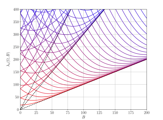
(a)

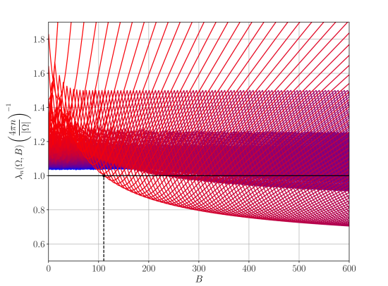
(b)

Figure 1: Eigenvalues for a disc of radius of $R=1/\sqrt{\pi}$ (and hence area $|D_{R}|=1$). Color of the curves fades from red to blue as $n$ increases. (a) Low eigenvalues over the field strength $B$. The dashed lines indicate the lines $\lambda=B$, $3B$ and $5B$. (b) The first 500 eigenvalues divided by $4\pi n/|D_{R}|$ plotted over the field strength $B$. The value $1.0$ associated with the lower bound from the non-magnetic Pólya conjecture is crossed for the first time at $B_{\mathrm{crit}}\approx 110.335$ by $\lambda_{11}(D_{R},B)$. This point is marked by a black dot and a dashed line.

2.2 Asymptotics for eigenvalue branches of the disc

Figure 1(a) displays the lowest few eigenvalues $\lambda_{n}(D_{R},B)$ over $B$ for a disc of unit area. It suggests that the eigenvalue branches have an asymptotically linear behavior as $B\rightarrow+\infty$ and there appear linearly growing sectors that only certain branches can populate. A detailed investigation of the eigenvalue branches $\lambda_{m,l}(B)$ has been carried out in the doctoral thesis of Son [23, Theorem 3.3.4] where it is proven that

$$\lim_{B\rightarrow+\infty}\frac{\lambda_{m,l}(B)}{B}=l+|l|+1+2(m-1).$$

Son posed the question for the asymptotic expression of the remainder $\lambda_{m,l}(B)/B-(l+|l|+1+2(m-1))$ which is equivalent to asking for the next terms in the asymptotic expansion of $\lambda_{m,l}(B)$. In the case of the ground state (which can be identified with the branch $\lambda_{1,0}(B)$), this question was already addressed by Helffer and Morame [15, Proposition 4.4] in 2001. However, their asymptotic expression is incorrect and was also mistakenly cited by Ekholm, Kovařík and Portmann [7] and Fournais and Helffer [11]. Helffer and Sundqvist [16] corrected the erroneous asymptotic from [15] by showing an asymptotic in the semi-classical setting via construction of trial states. Theorem 5.1 of [16] asserts that if $D_{R}$ is a disc of radius $R>0$, then for any $n\in\mathbb{N}$

$$\frac{\lambda_{n}(D_{R},B)}{B}-1=\frac{2}{(n-1)!}\left(\frac{BR^{2}}{2}\right)^{n}e^{-BR^{2}/2}(1+O(B^{-1}))\qquad\text{as }B\rightarrow+\infty.$$

Barbaroux et al. [3] gave a generalization of this result for non-constant magnetic fields and fairly generic domains.

This however does not fully answer the question about the second term in the asymptotic expansion of the eigenvalue branches $\lambda_{m,l}(B)$ for all $m\in\mathbb{N}$, $l\in\mathbb{Z}$. The construction of trial states only allows treating eigenvalues sorted in increasing order. As we will see with Corollary 4.2, the sorted eigenvalues $\lambda_{n}(\Omega,B)$ coincide with the eigenvalue branches $\lambda_{1,-(n-1)}(B)$ for large enough $B$, so the result by Helffer and Sundqvist only covers the case $m=1$ and $l\leq 0$.

Our first result gives the next term in the asymptotic expansion for all eigenvalue branches $\lambda_{m,l}(B)$ and therefore generalizes the result by Helffer and Sundqvist.

Theorem 2.1.

For any fixed $m\in\mathbb{N}$, $l\in\mathbb{Z}$ and $R>0$ holds

$$\frac{\lambda_{m,l}(B)}{B}>l+|l|+1+2(m-1)\qquad\text{for all }B>0$$

and

$$\frac{\lambda_{m,l}(B)}{B}-(l+|l|+1+2(m-1))=\frac{2}{\Gamma(|l|+m)\Gamma(m)}\left(\frac{BR^{2}}{2}\right)^{|l|+1+2(m-1)}e^{-\frac{BR^{2}}{2}}(1+O(B^{-1}))$$

as $B\rightarrow+\infty$.

We give the proof of Theorem 2.1 in Section 3. Note that the proof can be extended to gain more orders in the asymptotic expansion.

2.3 Spectral inequalities and sharpness

For the constant magnetic field, Erdös, Loss and Vougalter [8] proved that

$$\sum_{k=1}^{n}\lambda_{k}(\Omega,B)\geq\frac{2\pi n^{2}}{|\Omega|},\qquad n\in\mathbb{N},$$ (10)

for any $B\in\mathbb{R}$. Earlier, Li and Yau [19] had shown the inequality in the non-magnetic case. It was then realized that the Li-Yau bound is equivalent to Berezin’s bound by Legendre transformation, see e.g. [13, Chapter 3.5]. Similarly, (10) is equivalent to (5) for $\gamma=1$.

By the same reasoning as without magnetic field, the result by Erdös, Loss and Vougalter implies (5) with the excess factors $R_{\gamma}$ defined in the introduction and in particular

$$\lambda_{n}(\Omega,B)\geq\frac{1}{2}\cdot\frac{4\pi n}{|\Omega|},\qquad n\in\mathbb{N},B\in\mathbb{R},$$ (11)

for any domain $\Omega$. Compared to Pólya’s conjectured bound (2) for the non-magnetic case there appears an excess factor of $1/2$.

Our second main result is a proof of the sharpness of (11) for any domain $\Omega$ when $B$ is allowed to become large.

Theorem 2.2.

Let $\Omega\subset\mathbb{R}^{2}$ be a domain of finite measure. Then for any $\eta>0$ there exists some $B_{\eta}>0$ such that for any $B\geq B_{\eta}$ one has at least one eigenvalue $\lambda_{n}(\Omega,B)$ with

$$\frac{1}{2}\leq\lambda_{n}(\Omega,B)\left(\frac{4\pi n}{|\Omega|}\right)^{-1}\leq\frac{1}{2}+\eta.$$

We show Theorem 2.2 in Section 4. We first prove Theorem 2.2 in the case of discs by an explicit calculation. We then extend the result to disjoint unions of discs and finally any open domain $\Omega$ of finite measure by a domain inclusion argument.

As a consequence of the theorem, none of the excess factors $R_{\gamma}$, $\gamma\geq 0$, in (5) can be improved for any fixed domain. This is Frank’s sharpness result [12, Theorem 3.6] that was already mentioned in the introduction.

Corollary 2.3.

Let $\Omega\subset\mathbb{R}^{2}$ be a domain of finite measure and $\gamma\geq 0$. Then for any $\eta>0$, there exists some $B_{\eta}>0$ such that for any $B\geq B_{\eta}$ one finds some $\lambda>0$ with

$$R_{\gamma}-\eta\leq\frac{\mathrm{tr}(H_{B}^{\Omega}-\lambda)_{-}^{\gamma}}{L_{\gamma,2}^{\mathrm{cl}}|\Omega|\lambda^{1+\gamma}}\leq R_{\gamma}.$$ (12)

The proof of the corollary will be given right after the proof of Theorem 2.2 in Section 4.

Figure 1(b) illustrates Theorem 2.2 for the disc. It shows that once the field strength surpasses a critical value, the normalized quantities $\lambda_{n}(\Omega,B)(4\pi n/|\Omega|)^{-1}$ frequently drop below the constant one, indicated by a black line. This is exactly the case when the sorted eigenvalues $\lambda_{n}(\Omega,B)$ fall below the non-magnetic Pólya bound of $4\pi n/|\Omega|$. Theorem 2.2 asserts that any domain $\Omega$ features this kind of behavior and that

$$\lim_{B\rightarrow\infty}\;\inf_{n\in\mathbb{N}}\lambda_{n}(\Omega,B)\left(\frac{4\pi n}{|\Omega|}\right)^{-1}=\frac{1}{2},$$ (13)

i.e. the lower envelope of all curves in Figure 1(b) must converge to $1/2$ as $B\rightarrow\infty$. Our proof of Theorem 2.2 allows an estimate on the convergence speed of (13). For the disc, we provide an upper bound without proof in the appendix. We plan to publish its proof in a future article.

Remark.

Opposite to the strong magnetic field limit where Pólya’s non-magnetic bound fails, it is a striking feature of the figure that all eigenvalues considered appear to satisfy Pólya’s bound on a finite interval of small magnetic field strengths. More specifically, we see that for a disc with $|D_{R}|=1$, Pólya’s bound appears to be preserved if $B<B_{\mathrm{crit}}\approx 110.335$. By scaling, the same is the case for discs of radius $R>0$ when $B<B_{\mathrm{crit}}\cdot|D_{R}|^{-1}$. This can be rephrased as a condition on the magnetic flux

$$\phi=\frac{1}{2\pi}\int_{\Omega}B\,\mathrm{d}x=\frac{|\Omega|B}{2\pi},$$

The condition $B<B_{\mathrm{crit}}\cdot|D_{R}|^{-1}$ is equivalent to $\phi<B_{\mathrm{crit}}/(2\pi)\approx 17.56$. Guided by the numerics, we may ask: Is there actually a critical magnetic flux $\phi_{\mathrm{crit}}$ so that Pólya’s bound is preserved for $\phi<\phi_{\mathrm{crit}}$? Is it also true for domains of arbitrary shape?

3 Proof of Theorem 2.1

For completeness, we begin with a proof of the fact that

$$\lim_{B\rightarrow+\infty}\frac{\lambda_{m,l}(B)}{B}=l+|l|+1+2(m-1).$$

After that we compute the asymptotic expression of the remainder term.

Equation (8) relates eigenvalues for the magnetic Dirichlet Laplacian on the disc with roots of Kummer’s function. Statements about roots of $a\mapsto M(a,b,z)$ directly translate into properties of eigenvalues. We will therefore closely analyze Kummer’s function and its roots in the following. The arguments of Kummer’s function in (8) are always real-valued, so from now on the arguments $a,b$ and $z$ of Kummer’s function will be considered real numbers.

The existence of a limit of $\lambda_{m,l}(B)/B$ can be established by monotone convergence. For $\lambda\leq(l+|l|+1)B$ we have

$$\frac{1}{2}\left(l+|l|+1-\frac{\lambda}{B}\right)\geq 0$$

and thus

$$M\left(\frac{1}{2}\left(l+|l|+1-\frac{\lambda}{B}\right),|l|+1,\frac{BR^{2}}{2}\right)=1+\sum\limits_{k=1}^{\infty}\frac{\left(\frac{1}{2}\left(l+|l|+1-\frac{\lambda}{B}\right)\right)_{k}}{(|l|+1)_{k}k!}\left(\frac{BR^{2}}{2}\right)^{k}\geq 1,$$

as all summands in the series are non-negative. Therefore, (8) cannot be satisfied and $\lambda$ cannot be an eigenvalue. This means that any eigenvalue $\lambda_{m,l}(B)$ must fulfill

$$\frac{\lambda_{m,l}(B)}{B}>l+|l|+1.$$

Note that the roots $a_{m}(b,z)$ are strictly increasing with $z>0$ for any fixed $b>0$ and $m\in\mathbb{N}$, see e.g. [6, §17]. According to (9), this implies that all maps $B\mapsto\lambda_{m,l}(B)/B$ are strictly decreasing. By monotone convergence, the limit $\lim_{B\rightarrow+\infty}\lambda_{m,l}(B)/B$ exists and is bounded from below by $(l+|l|+1)$.

Let us now determine this limit. Let $b=|l|+1>0$ be fixed. For any $m\in\mathbb{N}_{0}$ we have

$$M(-m,b,z)=\sum\limits_{k=0}^{\infty}\frac{(-m)_{k}}{(b)_{k}k!}z^{k}=\sum\limits_{k=0}^{m}\frac{(-m)_{k}}{(b)_{k}k!}z^{k},$$

since $(-m)_{k}=0$ for $k>m$. The map $z\mapsto M(-m,b,z)$ is a (scaled Laguerre) polynomial in $z$ of degree $m$ and for real $z$ we have

$$M(-m,b,z)=\frac{(-m)_{m}}{(b)_{m}m!}z^{m}(1+O(z^{-1}))=\frac{(-1)^{m}}{(b)_{m}}z^{m}(1+O(z^{-1}))\qquad\text{as }z\rightarrow+\infty.$$

Thus, if $z^{*}>0$ is chosen large enough, one can enforce that $\text{sgn}(M(-m,b,z))=(-1)^{m}$ for all $z>z^{*}$. Let now $m^{\prime}\in\mathbb{N}$. One can choose $z^{*}>0$ large enough such that $\text{sgn}(M(-m,b,z^{*}))=(-1)^{m}$ for all integers $m$ with $0\leq m\leq m^{\prime}$. As $a\mapsto M(a,b,z)$ is continuous for fixed $z>z^{*}$, it must have at least one root in each of the intervals $(-m,-(m-1))$, $1\leq m\leq m^{\prime}$, by the intermediate value theorem. However, it is actually true that each of these intervals contains exactly one root. This is a consequence of intimate connection between roots of $a\mapsto M(a,b,z)$ and roots of $z\mapsto M(a,b,z)$ which is content of the next lemma. We will see that $a_{m}(b,z)$ must be bounded from above by $-(m-1)$.

To state the lemma, let us introduce some new notation. First, since $b$ is fixed, we suppress the parameter $b$ in the following and just write $a_{m}(z)$ for the negative roots of $a\mapsto M(a,b,z)$ instead of $a_{m}(b,z)$. Recall that for every fixed $z>0$ the roots $a_{m}(z)$ are sorted in decreasing order. The function $z\mapsto M(a,b,z)$ for $a<0$, $b>0$, has exactly $\lceil-a\rceil$ real, positive roots, see [24, §9], [6, §17] or [21, Section 13.9]. We sort the roots in increasing order and denote the $m$-th root by $z_{m}(a)$. Figure 2 shows the first few roots $a_{m}(z)$ and $z_{m}(a)$ for the case $b=1$. We will now proceed to prove the following lemma.

Lemma 3.1.

Let $a_{m}(z)$, $z_{m}(a)$ be defined as above. Then for all $m\in\mathbb{N}$

$$a_{m}(z)<-(m-1)\qquad\text{for all }z\in(0,\infty).$$

Moreover, $a_{m}:(0,\infty)\rightarrow(-\infty,-(m-1))$ is invertible and its inverse is given by $z_{m}:(-\infty,-(m-1))\rightarrow(0,\infty)$.

The lemma not only states that $a_{m}(z)$ can be inverted by some $z_{k}(a)$ but that the index $k$ is always be equal to $m$. Knowing this, the upper bound on the root $a_{m}(z)$ is owed to the fact that there are only $\lceil-a\rceil$ real, positive roots $z_{m}(a)$ for fixed $a$.

Lemma 3.1 appeared as part of Proposition 4.3.12 in the thesis of Son [23]. The importance of the lemma is two-fold. For one, it guarantees the upper bound $a_{m}(z)<-(m-1)$ that we need in this section. Secondly, we will make use of the characterization of the inverse of $a_{m}(z)$ in the proof of Theorem 2.2, see Corollary 4.1. For convenience of the reader, we give a self-contained proof of the lemma.

Proof.

First, note that all roots $a_{m}(z)$ and $z_{m}(a)$, $m\in\mathbb{N}$, are simple. For the roots $a_{m}(z)$, we already mentioned this fact before. The roots $z_{m}(a)$ are simple as well. This is because, if one of them were a multiple root, repeated use of Kummer’s equation would imply that this particular root is of infinite order. But viewed as a complex function, Kummer’s function is entire in $z$. A root of infinite order would imply that Kummer’s function is identical to the zero function which is a clear contradiction.

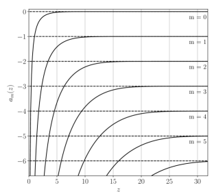
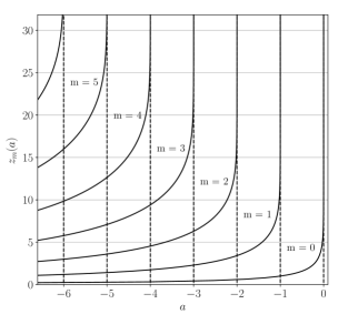
Figure 2: The first few roots $a_{m}(z)$ and $z_{m}(a)$ for $b=1$.

For fixed $a<0$ there are exactly $\lceil-a\rceil$ roots $z_{m}(a)$, which means that the $m$-th root $z_{m}(a)$ only exists for $a\in(-\infty,-(m-1))$. By the implicit function theorem, all maps $a_{m}$ and $z_{m}$, defined on $(0,\infty)$ resp. $(-\infty,-(m-1))$ are smooth functions. For now, we only know that the image of $a_{m}$ is contained in $(-\infty,0)$, because we do not have any constraints yet where the roots $a_{m}(z)$ lie other than that they are negative. We know $a_{m}$ is injective, since $a_{m}(z)$ is strictly increasing with $z$. We need to show that the image of $a_{m}$ is $(-\infty,-(m-1))$ and inverted by $z_{m}$.

Let $a\in(-\infty,0)$, $z\in(0,\infty)$. Note that $a$ is a root of $a^{\prime}\mapsto M(a^{\prime},b,z)$ if and only if $z$ is a root of $z^{\prime}\mapsto M(a,b,z^{\prime})$. This means that $a=a_{m}(z)$ only if $z=z_{k}(a)$ for some $k\in\mathbb{N}$, $1\leq k\leq\lceil-a\rceil$, and conversely $z=z_{k}(a)$ only if $a=a_{m}(z)$ for some $m\in\mathbb{N}$. We wrote $k$ because we do not know yet what the connection between $m$ and $k$ is. We now show that $m=k$ always holds. In other words, we show that

$$\text{if }a\in[-(m-1),0),\qquad \text{then}\qquad a=a_{m}(z)\text{ has no solution }z\in(0,\infty)$$

$$\text{and if }a\in(-\infty,-(m-1)),\qquad \text{then}\qquad a=a_{m}(z)\text{ if and only if }z=z_{m}(a).$$

Once this is shown, we have that the image of $a_{m}$ is contained in $(-\infty,-(m-1))$ and $z_{m}:(-\infty,-(m-1))\rightarrow(0,\infty)$ is the inverse of $a_{m}:(0,\infty)\rightarrow(-\infty,-(m-1))$ which is the assertion of the lemma.

We carry out an induction over $m$. For the start of the induction, let $a\in(-\infty,0)$ be arbitrary and suppose $a=a_{1}(z_{k}(a))$ for some integer $1<k\leq\lceil-a\rceil$. There must exist some integer $m\in\mathbb{N}$ such that $a=a_{m}(z_{1}(a))$. But then the sortings $a_{1}(z)>a_{2}(z)>...$ and $z_{1}(a)<z_{2}(a)<...$ and the strict monotonicity of $a_{1}(z)$ with respect to $z$ yields the contradiction

$$a=a_{m}(z_{1}(a))\leq a_{1}(z_{1}(a))<a_{1}(z_{k}(a))=a.$$

Therefore, for any $a\in(-\infty,0)$, $a=a_{1}(z)$ if and only if $z=z_{1}(a)$.

Let us now assume that there exists an $m^{\prime}\in\mathbb{N}$ such that for all $m$ with $1\leq m\leq m^{\prime}$ we have

$$\text{if }a\in[-(m-1),0),\qquad \text{then}\qquad a=a_{m}(z)\text{ has no solution }z\in(0,\infty)$$

$$\text{and if }a\in(-\infty,-(m-1)),\qquad \text{then}\qquad a=a_{m}(z)\text{ if and only if }z=z_{m}(a).$$

We need to show that

$$\text{if }a\in[-(({m^{\prime}+1})-1),0),\qquad \text{then}\qquad a=a_{m^{\prime}+1}(z)\text{ has no solution }z\in(0,\infty)$$

$$\text{and if }a\in(-\infty,-(({m^{\prime}+1})-1)),\qquad \text{then}\qquad a=a_{m^{\prime}+1}(z)\text{ if and only if }z=z_{m^{\prime}+1}(a).$$

Let $a\in(-\infty,0)$ be arbitrary and assume that we have a $z\in(0,\infty)$ with $a=a_{m^{\prime}+1}(z)$. We know that $z=z_{k}(a)$ for some integer $k$ satisfying $1\leq k\leq\lceil-a\rceil$. First of all, if $k\leq m^{\prime}$, then by induction assumption $a=a_{k}(z_{k}(a))$. But this leads to the contradiction

$$a=a_{m^{\prime}+1}(z_{k}(a))<a_{k}(z_{k}(a))=a,$$

because $k<m^{\prime}+1$. Thus, we must have $k\geq m^{\prime}+1$.

We can now discuss the solvability of $a=a_{m^{\prime}+1}(z)$ case-by-case.

Case 1: If $a\in[-(({m^{\prime}+1})-1),0)=[-m^{\prime},0)$, then $1\leq k\leq\lceil-a\rceil$ implies $k\leq m^{\prime}$ which contradicts $k\geq m^{\prime}+1$. Therefore, there is no solution $z\in(0,\infty)$ to $a=a_{m^{\prime}+1}(z)$.

Case 2: Consider $a\in(-\infty,-(({m^{\prime}+1})-1))=(-\infty,-m^{\prime})$.

Case 2.1: If $a\in[-m^{\prime}-1,-m^{\prime})$, then $m^{\prime}+1\leq k\leq\lceil-a\rceil$ implies $k=m^{\prime}+1$. Thus, $a=a_{m^{\prime}+1}(z)$ if and only if $z=z_{m^{\prime}+1}(a)$.

Case 2.2: If $a\in(-\infty,-m^{\prime}-1)$, then more than $m^{\prime}+1$ roots in $z$ exist, namely $z_{1}(a)$, …, $z_{\lceil-a\rceil}(a)$, so that $k$ could be larger than $m^{\prime}+1$. Suppose $k>m^{\prime}+1$. There must exist some integer $m\in\mathbb{N}$ such that $a=a_{m}(z_{m^{\prime}+1}(a))$. If $m<m^{\prime}+1$, then by the induction assumption $a=a_{m}(z_{m}(a))$ which leads to the contradiction

$$a=a_{m}(z_{m}(a))<a_{m}(z_{m^{\prime}+1}(a))=a.$$

If $m\geq m^{\prime}+1$, then

$$a=a_{m}(z_{m^{\prime}+1}(a))\leq a_{m^{\prime}+1}(z_{m^{\prime}+1}(a))<a_{m^{\prime}+1}(z_{k}(a))=a$$

which is again a contradiction. Hence, $k=m^{\prime}+1$ and for all $a\in(-\infty,-(({m^{\prime}+1})-1))$ holds $a=a_{m^{\prime}+1}(z)$ only if $z=z_{m^{\prime}+1}(a)$. This concludes the induction and the proof. ∎

We return to the proof of Theorem 2.1. By Lemma 3.1 we have $a_{m}(z)<-(m-1)$ for all $z\in(0,\infty)$. Since $a_{m}:(0,\infty)\rightarrow(-\infty,-(m-1))$ is strictly increasing and bijective, we must have $a_{m}(z)\rightarrow-(m-1)$ for $z\rightarrow+\infty$. These two fact show directly with (9) that

$$\frac{\lambda_{m,l}(B)}{B}>l+|l|+1+2(m-1)\qquad\text{for all }B>0$$

and

$$\lim_{B\rightarrow+\infty}\frac{\lambda_{m,l}(B)}{B}=l+|l|+1+2(m-1).$$

The lower bound is the first statement of Theorem 2.1.

We can now discuss the decay rate of the remainder $\lambda_{m,l}(B)/B-(l+|l|+1+2(m-1))$. For this, we fix $b=|l|+1$ and set $\varepsilon_{m}(z):=-(m-1)-a_{m}(z)$ where - as previously - $a_{m}(z)$ is the $m$-th negative root of $a\mapsto M(a,b,z)$ for $z>0$ and fixed $b>0$. By Lemma 3.1, $\varepsilon_{m}(z)$ is always positive. Since $a_{m}(z)\rightarrow-(m-1)$ for $z\rightarrow+\infty$, we know that $\varepsilon_{m}(z)=o(1)$ for $z\rightarrow+\infty$. We look for an asymptotic expression of $\varepsilon_{m}(z)$ as $z\rightarrow+\infty$, since this translates directly into an asymptotic expression for the remainder $\lambda_{m,l}(B)/B-(l+|l|+1+2(m-1))$.

First, we split the series that defines $M(a_{m}(z),b,z)$ into two parts. If

$$p_{m}(z) :=\sum\limits_{k=0}^{m-1}\frac{(-(m-1)-\varepsilon_{m}(z))_{k}}{(b)_{k}k!}z^{k},$$

$$q_{m}(z) :=\sum\limits_{k=m}^{\infty}\frac{(-(m-1)-\varepsilon_{m}(z))_{k}}{(b)_{k}k!}z^{k},$$

then

$$p_{m}(z)+q_{m}(z)=M(a_{m}(z),b,z)=0.$$

The reason why splitting the series at $k=m$ is helpful to gain an asymptotic expression for $\varepsilon_{m}(z)$ is that $q_{m}(z)$ contains all terms that have $\varepsilon_{m}(z)$ as a factor appearing in the Pochhammer symbol. We can factor out $\varepsilon_{m}(z)$ from $q_{m}(z)$ and write $q_{m}(z)=\varepsilon_{m}(z)\tilde{q}_{m}(z)$. Then,

$$\varepsilon_{m}(z)=-\frac{p_{m}(z)}{\tilde{q}_{m}(z)}=\left|\frac{p_{m}(z)}{\tilde{q}_{m}(z)}\right|$$

and the asymptotic behavior of $\varepsilon_{m}(z)$ is determined by $p_{m}(z)$ and $\tilde{q}_{m}(z)$. As we will see, both $|p_{m}(z)|$ and $|\tilde{q}_{m}(z)|$ tend to infinity as $z\rightarrow+\infty$, but at different speed. It remains to investigate their asymptotic behavior as $z\rightarrow+\infty$.

Let us first analyze the asymptotic behavior of $p_{m}(z)$. For $c\in\mathbb{R}$ and $k\in\mathbb{N}_{0}$ the function $x\mapsto(c+x)_{k}$ is a polynomial in $x$ and $(c+x)_{k}=(c)_{k}+O(x)$ as $x\rightarrow 0$. Now, because we already know that $\varepsilon_{m}(z)\rightarrow 0$ as $z\rightarrow+\infty$, this yields that $(-(m-1)-\varepsilon_{m}(z))_{k}=(-(m-1))_{k}(1+O(\varepsilon_{m}(z)))=(-(m-1))_{k}(1+o(1))$ as $z\rightarrow+\infty$ for any fixed $k\in\mathbb{N}_{0}$ and $m\in\mathbb{N}$. Therefore, $p_{m}(z)$ is asymptotically dominated by the term with $k=m-1$, or more precisely

$$p_{m}(z)=\frac{(-(m-1))_{m-1}}{(b)_{m-1}(m-1)!}z^{m-1}(1+o(1))=\frac{(-1)^{m-1}}{(b)_{m-1}}z^{m-1}(1+o(1))\qquad\text{as }z\rightarrow+\infty.$$ (14)

Let us now take a closer look at $q_{m}(z)$. Using $(b)_{i+j}=(b)_{i}(b+i)_{j}$ for $b\in\mathbb{R}$ and $i,j\in\mathbb{N}_{0}$ and $n!=(1)_{n}$ for $n\in\mathbb{N}_{0}$ yields

$$q_{m}(z) =\sum\limits_{k=m}^{\infty}\frac{(-(m-1)-\varepsilon_{m}(z))_{k}}{(b)_{k}k!}z^{k}$$

$$=(-(m-1)-\varepsilon_{m}(z))_{m}z^{m}\sum\limits_{k=m}^{\infty}\frac{(1-\varepsilon_{m}(z))_{k-m}}{(b)_{k}k!}z^{k-m}$$

$$=(-1)^{m}(1+\varepsilon_{m}(z))_{m-1}\varepsilon_{m}(z)z^{m}\sum\limits_{k=0}^{\infty}\frac{(1-\varepsilon_{m}(z))_{k}}{(b)_{k+m}(k+m)!}z^{k}$$

$$=(-1)^{m}(1+\varepsilon_{m}(z))_{m-1}\varepsilon_{m}(z)z^{m}\sum\limits_{k=0}^{\infty}\frac{(1)_{k}(1-\varepsilon_{m}(z))_{k}}{(b)_{m}(b+m)_{k}(1)_{m}(1+m)_{k}}\frac{z^{k}}{k!}$$

$$=\varepsilon_{m}(z)\tilde{q}_{m}(z).$$

where

$$\tilde{q}_{m}(z):=(-1)^{m}(1+\varepsilon_{m}(z))_{m-1}z^{m}\sum\limits_{k=0}^{\infty}\frac{(1)_{k}(1-\varepsilon_{m}(z))_{k}}{(b)_{m}(b+m)_{k}(1)_{m}(1+m)_{k}}\frac{z^{k}}{k!}.$$

Note, that if $z$ is large enough, then $\varepsilon_{m}(z)<1$, the summands in the series are positive and $\tilde{q}_{m}(z)$ has indeed the opposite sign of $p_{m}(z)$ as expected. We can rewrite $\tilde{q}_{m}(z)$ as

$$\tilde{q}_{m}(z)=\frac{(-1)^{m}(1+\varepsilon_{m}(z))_{m-1}z^{m}}{(1)_{m}(b)_{m}}\,{}_{2}F_{2}(1,1-\varepsilon_{m}(z);m+1,b+m;z)$$

where

$${}_{2}F_{2}(a,b;c,d;z)=\sum\limits_{k=0}^{\infty}\frac{(a)_{k}(b)_{k}}{(c)_{k}(d)_{k}}\frac{z^{k}}{k!},\qquad c,d\neq 0,-1,-2,...$$

is a generalized hypergeometric function, see for example [4, Volume I, Chapter IV] and [20, Chapter 3]. For given parameters $a,b,c,d$, the generalized hypergeometric function ${}_{2}F_{2}$ is an entire function in $z$ and is increasing in $a,b$ for $a,b>0$. For fixed $a,b,c,d$ we have

$${}_{2}F_{2}(a,b;c,d;z)=\frac{\Gamma(c)\Gamma(d)}{\Gamma(a)\Gamma(b)}z^{a+b-c-d}e^{z}(1+O(z^{-1}))\qquad\text{as }z\rightarrow+\infty,$$ (15)

see [20, Chapter 5.11.3] for reference. Let now be $0<\varepsilon<1$ arbitrary and let $z^{*}$ be large enough such that $\varepsilon_{m}(z)<\varepsilon$ for all $z>z^{*}$. Then $(1-\varepsilon)_{k}<(1-\varepsilon_{m}(z))_{k}$ for all $k\in\mathbb{N}$ and all $z>z^{*}$, therefore

$${}_{2}F_{2}(1,1-\varepsilon_{m}(z);m+1,b+m;z)>{}_{2}F_{2}(1,1-\varepsilon;m+1,b+m;z)>0$$

for all $z>z^{*}$ and

$$|\tilde{q}_{m}(z)| =\frac{(1+\varepsilon_{m}(z))_{m-1}z^{m}}{(1)_{m}(b)_{m}}\,{}_{2}F_{2}(1,1-\varepsilon_{m}(z);m+1,b+m;z)$$

$$>\frac{(1)_{m-1}z^{m}}{(1)_{m}(b)_{m}}\,{}_{2}F_{2}(1,1-\varepsilon;m+1,b+m;z)$$

$$=\frac{z^{m}}{m(b)_{m}}\frac{\Gamma(m+1)\Gamma(b+m)}{\Gamma(1-\varepsilon)}z^{1+1-\varepsilon-m-1-b-m}e^{z}(1+O(z^{-1}))\qquad\text{as }z\rightarrow+\infty$$

$$=\frac{\Gamma(m)\Gamma(b+m)}{(b)_{m}\Gamma(1-\varepsilon)}z^{1-\varepsilon-b-m}e^{z}(1+O(z^{-1}))\qquad\text{as }z\rightarrow+\infty.$$

Combining this with (14), we get

$$\varepsilon_{m}(z)=\left|\frac{p_{m}(z)}{\tilde{q}_{m}(z)}\right| \leq\frac{(b)_{m}\Gamma(1-\varepsilon)}{(b)_{m-1}\Gamma(m)\Gamma(b+m)}z^{b+2(m-1)+\varepsilon}e^{-z}(1+o(1))\qquad\text{as }z\rightarrow+\infty$$

$$=\frac{\Gamma(1-\varepsilon)}{\Gamma(m)\Gamma(b+m-1)}z^{b+2(m-1)+\varepsilon}e^{-z}(1+o(1))\qquad\text{as }z\rightarrow+\infty.$$

and therefore for any $\varepsilon>0$

$$\varepsilon_{m}(z)=O(z^{b+2(m-1)+\varepsilon}e^{-z})\qquad\text{as }z\rightarrow+\infty.$$ (16)

This is not the asymptotic expression for $\varepsilon_{m}(z)$ we want, but it is a good upper bound on its decay rate. To find the asymptotic expression for $\varepsilon_{m}(z)$, we can feed back this upper bound in our calculation of asymptotics of $p_{m}(z)$ and $\tilde{q}_{m}(z)$ to improve them further.

With the aid of (16), we now know that for any $\varepsilon>0$ and any fixed $k\in\mathbb{N}_{0}$

$$(-(m-1)-\varepsilon_{m}(z))_{k}z^{k}=(-(m-1))_{k}z^{k}(1+O(z^{b+2(m-1)+\varepsilon}e^{-z}))\qquad\text{as }z\rightarrow+\infty.$$

Compared to (14), this leads to the improved asymptotic

$$p_{m}(z)=\sum\limits_{k=0}^{m-1}\frac{(-(m-1))_{k}}{(b)_{k}k!}z^{k}+o(1)\qquad\text{as }z\rightarrow+\infty.$$ (17)

Next, we improve our lower bound for $|\tilde{q}_{m}(z)|$. We note that for any $k\in\mathbb{N}$

$$(1-x)_{k}=\sum\limits_{j=0}^{k}c_{k,j}x^{j}$$

where $c_{k,j}$ are suitable coefficients with $c_{k,0}=(1)_{k}$ and $\text{sgn}(c_{k,j})=(-1)^{j}$. For $x=-1$, we see that

$$\sum_{j=0}^{k}|c_{k,j}|=\sum_{j=0}^{k}c_{k,j}(-1)^{j}=(2)_{k}$$

and in particular $|c_{k,j}|\leq(2)_{k}$ for all $0\leq j\leq k$. Using this, we deduce that

$$|{}_{2}F_{2}(1,1;m+1,b+m;z)-{}_{2}F_{2}(1,1-\varepsilon_{m}(z);m+1,b+m;z)|$$

$$= \;\left|\sum\limits_{k=1}^{\infty}\frac{(1)_{k}[(1)_{k}-(1-\varepsilon_{m}(z))_{k}]}{(b+m)_{k}(1+m)_{k}}\frac{z^{k}}{k!}\right|$$

$$\leq \;\sum\limits_{k=1}^{\infty}\sum\limits_{j=1}^{k}\frac{(1)_{k}|c_{k,j}|(\varepsilon_{m}(z))^{j}}{(b+m)_{k}(1+m)_{k}}\frac{z^{k}}{k!}$$

$$\leq \;\sum\limits_{j=1}^{\infty}(\varepsilon_{m}(z))^{j}\sum\limits_{k=j}^{\infty}\frac{(1)_{k}(2)_{k}}{(b+m)_{k}(1+m)_{k}}\frac{z^{k}}{k!}.$$

Now, with (15) follows

$$\sum\limits_{k=j}^{\infty}\frac{(1)_{k}(2)_{k}}{(b+m)_{k}(1+m)_{k}}\frac{z^{k}}{k!} \leq\sum\limits_{k=0}^{\infty}\frac{(1)_{k}(2)_{k}}{(b+m)_{k}(1+m)_{k}}\frac{z^{k}}{k!}$$

$$={}_{2}F_{2}(1,2;m+1,b+m;z)$$

$$=O(z^{-b-2(m-1)}e^{z})\qquad\text{as }z\rightarrow+\infty$$

and with (16) we get

$$\sum\limits_{j=1}^{\infty}(\varepsilon_{m}(z))^{j}\sum\limits_{k=j}^{\infty}\frac{(1)_{k}(2)_{k}}{(b+m)_{k}(1+m)_{k}}\frac{z^{k}}{k!}\leq \;\frac{\varepsilon_{m}(z)}{1-\varepsilon_{m}(z)}\,{}_{2}F_{2}(1,2;m+1,b+m;z)$$

$$= \;O(z^{\varepsilon})\qquad\text{as }z\rightarrow+\infty$$

with the $\varepsilon$ coming from (16). Hence, we can improve the previous estimate of $|\tilde{q}_{m}(z)|$ to

$$|\tilde{q}_{m}(z)| =\frac{(1+\varepsilon_{m}(z))_{m-1}z^{m}}{(1)_{m}(b)_{m}}\,{}_{2}F_{2}(1,1-\varepsilon_{m}(z);m+1,b+m;z)$$

$$\geq\frac{(1)_{m-1}z^{m}}{(1)_{m}(b)_{m}}\,({}_{2}F_{2}(1,1;m+1,b+m;z)+O(z^{\varepsilon}))$$

$$=\frac{\Gamma(m)\Gamma(b+m)}{(b)_{m}}z^{1-b-m}e^{z}(1+O(z^{-1}))\qquad\text{as }z\rightarrow+\infty$$

which gives with (17)

$$\varepsilon_{m}(z)=\left|\frac{p_{m}(z)}{\tilde{q}_{m}(z)}\right|\leq\frac{1}{\Gamma(m)\Gamma(b+m-1)}z^{b+2(m-1)}e^{-z}(1+O(z^{-1}))\qquad\text{as }z\rightarrow+\infty.$$

This upper bound is the asymptotic expression we are looking for. It is not difficult to estimate $\tilde{q}_{m}(z)$ also from above by

$$|\tilde{q}_{m}(z)| \leq\frac{(1)_{m-1}z^{m}}{(1)_{m}(b)_{m}}(1+O(z^{-1}))\,{}_{2}F_{2}(1,1;m+1,b+m;z)$$

$$=\frac{\Gamma(m)\Gamma(b+m)}{(b)_{m}}z^{1-b-m}e^{z}(1+O(z^{-1}))\qquad\text{as }z\rightarrow+\infty$$

which then yields with (17) the corresponding lower bound

$$\varepsilon_{m}(z)=\left|\frac{p_{m}(z)}{\tilde{q}_{m}(z)}\right| \geq\frac{(b)_{m}}{(b)_{m-1}\Gamma(b+m)(m-1)!}z^{b+2(m-1)}e^{-z}(1+O(z^{-1}))\qquad\text{as }z\rightarrow+\infty$$

$$=\frac{1}{\Gamma(m)\Gamma(b+m-1)}z^{b+2(m-1)}e^{-z}(1+O(z^{-1}))\qquad\text{as }z\rightarrow+\infty.$$

Putting both bounds for $\varepsilon_{m}(z)$ together we have established

$$\varepsilon_{m}(z)=\frac{1}{\Gamma(m)\Gamma(b+m-1)}z^{b+2(m-1)}e^{-z}(1+O(z^{-1}))\qquad\text{as }z\rightarrow+\infty.$$ (18)

Finally, when we set $b=|l|+1$, $z=BR^{2}/2$ and employ the relation

$$\frac{\lambda_{m,l}(B)}{B}=l+|l|+1-2a_{m}\left(\frac{BR^{2}}{2}\right)=l+|l|+1+2(m-1)+2\varepsilon\left(\frac{BR^{2}}{2}\right),$$

our result (18) becomes the second statement of the theorem.

4 Proof of Theorem 2.2 and Corollary 2.3

We begin with the proof of Theorem 2.2. Given $\eta>0$, we need to find an eigenvalue $\lambda_{n}(\Omega,B)$ that satisfies

$$\lambda_{n}(\Omega,B)\leq\left(\frac{1}{2}+\eta\right)\frac{4\pi n}{|\Omega|}$$ (19)

for some $n=n(B)$ when $B$ is large enough. The index $n(B)$ cannot be chosen independent of $B$ but generally needs to increase with $B$. This is because $\lambda_{n}(\Omega,B)\geq B$ for any $n\in\mathbb{N}$ (for discs, this follows from Theorem 2.1, but for general domains $\Omega$, see e.g. [11, Lemma 1.4.1]) and therefore the bound (19) cannot be satisfied for

$$n<\left(\frac{1}{2}+\eta\right)^{-1}\frac{|\Omega|B}{4\pi}.$$

We will see that one can choose $n(B)$ linearly increasing with $B$.

The proof of Theorem 2.2 is divided into three steps. First, we show the assertion of the theorem in the case where $\Omega$ is a disc. We are then able to lift the result from discs to unions of disjoint discs. The generalization to arbitrary domains is done with coverings by unions of disjoint discs and a domain inclusion argument. We conclude the section by proving the corresponding result for Riesz means.

4.1 Proof of Theorem 2.2 for discs

Although we know the eigenvalue branches $\lambda_{m,l}(B)$ for the disc in terms of roots of Kummer’s function, there remains the difficulty of relating the eigenvalue branches $\lambda_{m,l}(B)$ to the sorted eigenvalues $\lambda_{n}(D_{R},B)$. We need to identify $\lambda_{m,l}(B)$ with $\lambda_{n}(D_{R},B)$ for certain $n$ and also find estimates on the branches $\lambda_{m,l}(B)$. We will gain such estimates from a further investigation of the Kummer function.

It will suffice for us to characterize all eigenvalues $\lambda_{n}(D_{R},B)\leq 3B$. Theorem 2.1 tells us that $\lambda_{m,l}(B)>3B$ for $m\geq 2$ or $l>0$, so all eigenvalues $\lambda_{n}(D_{R},B)\leq 3B$ must correspond to eigenvalue branches $\lambda_{1,l}(B)$ with $l\leq 0$. As seen in Figure 1(a), the number of branches $\lambda_{1,l}(B)\leq 3B$ depends on the field strength. We can count these branches by counting the intersection points between $\lambda_{1,l}(B)$ and the line $\lambda=3B$. In general, intersections of the eigenvalue branches $\lambda_{m,l}(B)$ with lines $\lambda=(l+|l|+1+2k)B$, $k\in\mathbb{N}$, can be identified with help of Lemma 3.1.

Recall that $\lambda_{m,l}(B)/B$ is strictly decreasing, so $\lambda_{m,l}(B)$ has at most one intersection with a line $\lambda=(l+|l|+1+2k)B$, $k\in\mathbb{N}$. By the lower bound given in Theorem 2.1, the branch $\lambda_{m,l}(B)$ has no intersection with $\lambda=(l+|l|+1+2k)B$ if $k\leq m-1$. If $k\geq m$, there is an intersection and Lemma 3.1 yields the following.

Corollary 4.1.

Let $m\in\mathbb{N}$, $l\in\mathbb{Z}$ and $k\in\mathbb{N}$, $k\geq m$. Then $\lambda_{m,l}(B)=(l+|l|+1+2k)B$ if and only if $B=2z_{m}(-k,|l|+1)/R^{2}$. Here, $z_{m}(a,b)$ denotes the $m$-th positive root of $z\mapsto M(a,b,z)$.

For the proof, recall also that we denoted the $m$-th negative root of $a\mapsto M(a,b,z)$ earlier by $a_{m}(b,z)$, sorted in decreasing order.

Proof.

According to (9), $\lambda_{m,l}(B)$ is related to the root $a_{m}(b,z)$ by

$$\lambda_{m,l}(B)=\left(l+|l|+1-2a_{m}\left(|l|+1,\frac{BR^{2}}{2}\right)\right)B.$$

Therefore, $\lambda_{m,l}(B)=(l+|l|+1+2k)B$ if and only if

$$a_{m}\left(|l|+1,\frac{BR^{2}}{2}\right)=-k.$$

Finally, since $z_{m}$ is the inverse of $a_{m}$ with respect to $a\in(-\infty,-(m-1))$ for any fixed $b>0$ by Lemma 3.1 and $-k\in(-\infty,-(m-1))$ for $k\geq m$, we see that

$$a_{m}\left(|l|+1,\frac{BR^{2}}{2}\right)=-k\qquad\text{if and only if}\qquad\frac{BR^{2}}{2}=z_{m}(-k,|l|+1).$$

∎

For $k\in\mathbb{N}$, the power series of $M(-k,b,z)$ turns into a polynomial of degree $k$ which allows explicit computation of the roots $z_{m}(-k,b)$ for low $k$. In particular, if $k=1$, the polynomial $M(-1,b,z)=1-z/b$ is linear and its only root is $z=b$. This means $z_{1}(-1,b)=b$ and $a_{1}(b,b)=-1$. With $b=|l|+1$, the corollary implies $\lambda_{1,l}(B)=3B$ if and only if $l\leq 0$ and

$$B=\frac{2z_{1}(-1,|l|+1)}{R^{2}}=\frac{2}{R^{2}}(|l|+1).$$

This allows us to give a simple characterization of sorted eigenvalues $\lambda_{n}(D_{R},B)$.

Corollary 4.2.

Let $n\in\mathbb{N}$. If $B\geq 2n/R^{2}$, then

$$\lambda_{n}(D_{R},B)=\lambda_{1,-(n-1)}(B).$$

Proof.

We have just shown with Corollary 4.1 that

$$\lambda_{1,-(n-1)}(B)=3B\qquad\text{if and only if }\qquad B=\frac{2n}{R^{2}},$$

thus, by strict monotonicity of $\lambda_{1,l}(B)/B$ with respect to $B$, we have $\lambda_{1,-(n-1)}(B)\leq 3B$ for $B\geq 2n/R^{2}$. Due to the fact that for any $B>0$

$$\lambda_{1,l^{\prime}}(B)>\lambda_{1,l}(B)\qquad\text{for }l^{\prime}<l\leq 0,$$

see [23, Theorem 3.3.4], we get

$$\lambda_{1,0}(B)<\lambda_{1,-1}(B)<...<\lambda_{1,-(n-1)}(B)\leq 3B\qquad\text{for }B\geq\frac{2n}{R^{2}}$$

and $\lambda_{1,l}(B)>\lambda_{1,-(n-1)}(B)$ for any $l\leq-n$. Recall that by Theorem 2.1, if $m\geq 2$ or $l>0$, then $\lambda_{m,l}(B)>3B$ and hence $\lambda_{m,l}(B)>\lambda_{1,-(n-1)}(B)$ if $B\geq 2n/R^{2}$. This shows that if $B\geq 2n/R^{2}$, there are no smaller eigenvalues than $\lambda_{1,0}(B)$, …, $\lambda_{1,-(n-1)}(B)$ and since they are sorted by magnitude, we can identify them with $\lambda_{1}(D_{R},B)$, …, $\lambda_{n}(D_{R},B)$. ∎

Let us now derive estimates for eigenvalue branches $\lambda_{1,l}(B)$, $l\leq 0$. First, we show the following lemma concerning Kummer’s function.

Lemma 4.3.

Let $0<\delta<1$ and $\varepsilon>0$. There exists $b_{\delta,\varepsilon}>0$ such that for any $b>b_{\delta,\varepsilon}$

$$M(-\delta,b,(1+\varepsilon)b)<0.$$

Proof.

First observe that

$$M(-\delta,b,(1+\varepsilon)b) =1+\sum\limits_{k=1}^{\infty}\frac{(-\delta)_{k}}{k!}\frac{b^{k}}{(b)_{k}}(1+\varepsilon)^{k}$$

where the series only sums negative terms when $0<\delta<1$. The appearing series converges, however the series

$$\sum\limits_{k=1}^{\infty}\frac{(-\delta)_{k}}{k!}(1+\varepsilon)^{k},$$

where we replaced the $b$ dependent terms by one, is divergent for any $\varepsilon>0$. It tends to $-\infty$, since all summands are negative and the radius of convergence of the power series

$$\sum\limits_{k=1}^{\infty}\frac{(-\delta)_{k}}{k!}z^{k}$$

is

$$R=\left(\lim_{k\rightarrow+\infty}\left(\frac{(-\delta)_{k}}{k!}\right)^{\frac{1}{k}}\right)^{-1}=\left(\lim_{k\rightarrow+\infty}\left(\frac{\Gamma(-\delta+k)}{\Gamma(-\delta)\Gamma(k+1)}\right)^{\frac{1}{k}}\right)^{-1}=1.$$

We can therefore choose some $c\in(0,1)$ and then some large $N\in\mathbb{N}$ such that

$$c\sum\limits_{k=1}^{N}\frac{(-\delta)_{k}}{k!}(1+\varepsilon)^{k}<-1.$$

Furthermore, for any fixed $k\geq 1$ holds

$$\frac{b^{k}}{(b)_{k}}\rightarrow 1\qquad\text{as }b\rightarrow+\infty,$$

thus there exists $b_{\delta,\varepsilon}>0$ such that for $b>b_{\delta,\varepsilon}$

$$\frac{b^{k}}{(b)_{k}}\geq c\qquad\text{for all }k=1,...,N.$$

Hence, for $b>b_{\delta,\varepsilon}$

$$M(-\delta,b,(1+\varepsilon)b)=1+\sum\limits_{k=1}^{\infty}\frac{(-\delta)_{k}}{k!}\frac{b^{k}}{(b)_{k}}(1+\varepsilon)^{k}\leq 1+c\sum\limits_{k=1}^{N}\frac{(-\delta)_{k}}{k!}(1+\varepsilon)^{k}<0.$$

and we have shown the lemma. ∎

The lemma implies a bound on the roots in $a$ of Kummer’s function and therefore on eigenvalue branches. Together with $M(0,b,(1+\varepsilon)b)=1>0$ we see that for any $b>b_{\delta,\varepsilon}$, the map $a\mapsto M(a,b,(1+\varepsilon)b)$ has at least one root in $(-\delta,0)$ by the intermediate value theorem. In particular, we have

$$-\delta<a_{1}(b,(1+\varepsilon)b)<0\qquad\text{for }b>b_{\delta,\varepsilon}.$$ (20)

Again, recall that $a_{1}(b,(1+\varepsilon)b)$ relates to the eigenvalues $\lambda_{1,l}(B)$ via (9). When setting $b=|l|+1$ for $l\leq 0$ we see that

$$\frac{\lambda_{1,l}(B_{|l|+1})}{B_{|l|+1}}=1-2a_{1}(|l|+1,(1+\varepsilon)(|l|+1))$$

where the magnetic field strength $B_{|l|+1}$ is given by

$$B_{|l|+1}=\frac{2}{R^{2}}(1+\varepsilon)(|l|+1).$$

But then (20) implies that

$$\frac{\lambda_{1,l}(B_{|l|+1})}{B_{|l|+1}}\leq 1+2\delta\qquad\text{for any }l\leq 0,|l|+1>b_{\delta,\varepsilon}$$

and since $\lambda_{1,l}(B)/B$ is strictly decreasing with $B$, we have

$$\frac{\lambda_{1,l}(B)}{B}\leq 1+2\delta\qquad\text{for any }B\geq B_{|l|+1}\text{ and }l\leq 0,|l|+1>b_{\delta,\varepsilon}.$$ (21)

With (21) at hand, we are almost done. It remains to bring $B$ to the right side, choose $\delta$ and $\varepsilon$ appropriately and use Corollary 4.2 to identify $\lambda_{1,-(n-1)}(B)$ with $\lambda_{n}(D_{R},B)$.

Let now $\eta>0$ be arbitrary. Choose $\varepsilon>0$ and $0<\delta<1$ small enough such that $(1+2\delta)(1+\varepsilon)<1+2\eta$. After that choose $b^{*}\geq b_{\delta,\varepsilon}$ large enough such that

$$(1+2\delta)(1+\varepsilon)\left(1+\frac{1}{b^{*}}\right)\leq 1+2\eta.$$

Assume $|l|+1>b^{*}$ and

$$B=\frac{2}{R^{2}}(1+\tilde{\varepsilon})(|l|+1),\qquad\text{where }\tilde{\varepsilon}\in\left[\varepsilon,\varepsilon+\frac{1+\varepsilon}{b^{*}}\right].$$ (22)

Since $\tilde{\varepsilon}\geq\varepsilon$, we have $B\geq B_{|l|+1}$ and therefore (21) holds. Hence, it follows that

$$\lambda_{1,l}(B) \leq(1+2\delta)B=(1+2\delta)\frac{2}{R^{2}}(1+\tilde{\varepsilon})(|l|+1)$$

$$\leq(1+2\delta)\left(1+\varepsilon+\frac{1+\varepsilon}{b^{*}}\right)\frac{2\pi}{|D_{R}|}(|l|+1)$$

$$=(1+2\delta)(1+\varepsilon)\left(1+\frac{1}{b^{*}}\right)\frac{2\pi}{|D_{R}|}(|l|+1)$$

$$\leq(1+2\eta)\frac{2\pi}{|D_{R}|}(|l|+1).$$

Note that if $|l|+1>b^{*}$ and $B\in[B_{|l|+1},B_{|l|+2}]$ then $B$ can be written as in (22) and thus we have shown that

$$\lambda_{1,l}(B)\leq(1+2\eta)\frac{2\pi}{|D_{R}|}(|l|+1),\qquad\text{for }B\in[B_{|l|+1},B_{|l|+2}],\;l\leq 0,\;|l|+1>b^{*}.$$

Now let $n=-l+1=|l|+1$. Then $B\in[B_{|l|+1},B_{|l|+2}]$ implies $B>2n/R^{2}$ and therefore by Corollary 4.2

$$\lambda_{n}(D_{R},B)=\lambda_{1,-(n-1)}(B)=\lambda_{1,l}(B)\leq(1+2\eta)\frac{2\pi}{|D_{R}|}(|l|+1)=\left(\frac{1}{2}+\eta\right)\frac{4\pi n}{|D_{R}|}$$ (23)

for $B\in[B_{n},B_{n+1}],\;n>b^{*}$. The desired inequality hence always holds for some eigenvalue if $B\geq\min_{n>b^{*}}B_{n}$.

4.2 Proof of Theorem 2.2 for disjoint unions of finitely many discs

Let $\eta>0$ be arbitrary. Let $N\in\mathbb{N}$ and $\Omega=\Omega_{1}\cup...\cup\Omega_{N}$ be the disjoint union of $N$ discs $\Omega_{i}=D_{R_{i}}$ with radii $R_{i}>0$. Then of course $|\Omega|=|\Omega_{1}|+...+|\Omega_{N}|=\pi\sum_{i=1}^{N}R_{i}^{2}$. By the previous proof for a single disc, we can choose a small $\varepsilon>0$ so that for all $i$ exist $b^{*}_{i}$ such that

$$\lambda_{n}(\Omega_{i},B)\leq(1+2\eta)\frac{2\pi n}{|\Omega_{i}|},\qquad\text{for }B\in[B_{n}^{(i)},B_{n+1}^{(i)}],\;n>b^{*}_{i},$$

where

$$B_{n}^{(i)}=\frac{2}{R_{i}^{2}}(1+\varepsilon)n.$$

Let $\eta^{\prime}>0$ and let $B_{\eta^{\prime}}>0$ be large enough such that

$$\frac{1}{1-\frac{2\pi(1+\varepsilon)N}{|\Omega|B}}\leq 1+\eta^{\prime}$$

for $B\geq B_{\eta^{\prime}}$. Then assume $B\geq\max\{\max_{1\leq i\leq N}B_{{\lceil b_{i}^{*}\rceil}}^{(i)},B_{\eta^{\prime}}\}$. For such $B$, there exists for all $i$ an $n_{i}$ with $B\in[B_{n_{i}}^{(i)},B_{n_{i}+1}^{(i)}]$ and we have seen that for this $n_{i}$ holds

$$\lambda_{n_{i}}(\Omega_{i},B)\leq(1+2\eta)\frac{2\pi n_{i}}{|\Omega_{i}|}.$$

The spectrum of $\Omega$ is just the union of the spectra of all $\Omega_{i}$, so for any $i$ exists an $n_{i}^{\prime}$ such that $\lambda_{n_{i}^{\prime}}(\Omega,B)=\lambda_{n_{i}}(\Omega_{i},B)$. We now let $n:=\max_{1\leq i\leq N}n_{i}^{\prime}$ so that $\lambda_{n}(\Omega,B)$ is the eigenvalue of $\Omega$ whose index corresponds to the largest of the eigenvalues $\lambda_{n_{i}}(\Omega_{i},B)$. The index of the maximizing component shall be denoted by $i^{*}$ so that we have $\lambda_{n}(\Omega,B)=\lambda_{n_{i^{*}}}(\Omega_{i^{*}},B)$. By the choice of $n$ we necessarily have $n\geq\sum_{i=1}^{N}n_{i}$. With this, we observe that

$$\lambda_{n}(\Omega,B)=\lambda_{n_{i^{*}}}(\Omega_{i^{*}},B) \leq(1+2\eta)\frac{2\pi n_{i^{*}}}{|\Omega_{i^{*}}|}=\frac{n_{i^{*}}}{n}\frac{|\Omega|}{|\Omega_{i^{*}}|}\left(\frac{1}{2}+\eta\right)\frac{4\pi n}{|\Omega|},$$

so all that remains to show is that $\frac{n_{i^{*}}}{n}\frac{|\Omega|}{|\Omega_{i^{*}}|}$ is close to one. From $B\in[B_{n_{i}}^{(i)},B_{n_{i}+1}^{(i)}]$ follows

$$\frac{BR_{i}^{2}}{2(1+\varepsilon)}-1\leq n_{i}\leq\frac{BR_{i}^{2}}{2(1+\varepsilon)}$$ (24)

for any $i$. Summing these inequalities over $i$ yields

$$\frac{B\sum_{i=1}^{N}R_{i}^{2}}{2(1+\varepsilon)}-N\leq\sum_{i=1}^{N}n_{i}\leq\frac{B\sum_{i=1}^{N}R_{i}^{2}}{2(1+\varepsilon)}.$$ (25)

Since $n\geq\sum_{i=1}^{N}n_{i}$, the inequalities (24) and (25) imply

$$\frac{n_{i^{*}}}{n}\leq\frac{\frac{BR_{i^{*}}^{2}}{2(1+\varepsilon)}}{\frac{B\sum_{i=1}^{N}R_{i}^{2}}{2(1+\varepsilon)}-N}=\frac{|\Omega_{i^{*}}|}{|\Omega|-\frac{2\pi(1+\varepsilon)N}{B}}$$

and thus

$$\frac{n_{i^{*}}}{n}\frac{|\Omega|}{|\Omega_{i^{*}}|}\leq\frac{1}{1-\frac{2\pi(1+\varepsilon)N}{|\Omega|B}}\leq 1+\eta^{\prime}.$$

Hence, we have

$$\lambda_{n}(\Omega,B)\leq(1+\eta^{\prime})\left(\frac{1}{2}+\eta\right)\frac{4\pi n}{|\Omega|}.$$

Because $\eta>0$ and $\eta^{\prime}>0$ were arbitrary, this proves the assertion if $\Omega$ is a disjoint union of finitely many discs.

4.3 Proof of Theorem 2.2 for general domains

For the final step, we take advantage of the domain inclusion principle. This principle is well-known for the non-magnetic Dirichlet Laplacian and states that eigenvalues increase under domain inclusion. The same holds with a constant magnetic field.

Lemma 4.4 (Domain inclusion principle).

Let $\Omega,\Omega^{\prime}$ be open domains of finite measure with $\Omega^{\prime}\subset\Omega$ and $B\geq 0$. Then

$$\lambda_{n}(\Omega^{\prime},B)\geq\lambda_{n}(\Omega,B)\qquad\text{for }n\in\mathbb{N}.$$

Proof.

Since $C_{0}^{\infty}(\Omega^{\prime})\subset C_{0}^{\infty}(\Omega)$ by trivial extension, the form closure of $C_{0}^{\infty}(\Omega^{\prime})$ w.r.t. the quadratic form of the magnetic Laplacian can be embedded in the form closure of $C_{0}^{\infty}(\Omega)$. The min-max-principle then shows the inequality between the eigenvalues. ∎

Let now $\Omega$ be any open set of finite measure. By Vitali’s covering theorem there exists a countable collection of pairwise disjoint open discs $\{\Omega_{i}\}_{i=1}^{\infty}$ such that $\Omega_{i}\subset\Omega$ for all $i\in\mathbb{N}$ and

$$\left|\Omega\setminus\bigcup_{i=1}^{\infty}\Omega_{i}\right|=0.$$

This means in particular that

$$\left|\bigcup_{i=1}^{N}\Omega_{i}\right|\rightarrow|\Omega|\qquad\text{as }N\rightarrow+\infty.$$

In other words, for any $\eta^{\prime}>0$ exists $\Omega^{\prime}\subset\Omega$, $\Omega^{\prime}$ being a disjoint union of finitely many discs, with $\dfrac{|\Omega|}{|\Omega^{\prime}|}\leq 1+\eta^{\prime}$. We have for $B$ large enough that for some $n$ holds

$$\lambda_{n}(\Omega^{\prime},B)\leq(1+2\eta)\frac{2\pi n}{|\Omega^{\prime}|}.$$

But then by domain monotonicity we arrive with such a disjoint union of discs $\Omega^{\prime}$ at

$$\lambda_{n}(\Omega,B)\leq\lambda_{n}(\Omega^{\prime},B)\leq(1+2\eta)\frac{2\pi n}{|\Omega^{\prime}|}\leq(1+2\eta)\dfrac{|\Omega|}{|\Omega^{\prime}|}\frac{2\pi n}{|\Omega|}=(1+\eta^{\prime})\left(\frac{1}{2}+\eta\right)\frac{4\pi n}{|\Omega|}.$$

Again, since $\eta$ and $\eta^{\prime}>0$ were arbitrary, this shows the assertion for general $\Omega$ and finishes the proof.

4.4 Proof of Corollary 2.3

Let $\eta>0$ be arbitrary. Choose $\eta^{\prime}>0$ small enough such that $2-\eta<2(1+2\eta^{\prime})^{-1}$. By Theorem 2.2, there exists $B_{\eta^{\prime}}>0$ such that for any $B\geq B_{\eta^{\prime}}$ exists an $n$ with

$$2-\eta<2(1+2\eta^{\prime})^{-1}\leq\frac{4\pi n}{|\Omega|\lambda_{n}(\Omega,B)}\leq 2.$$

Recall that $R_{0}=2$ and $L_{0,2}^{\mathrm{cl}}=1/4\pi$. Thus, letting $\lambda\searrow\lambda_{n}(\Omega,B)$, we get for any $B\geq B_{\eta^{\prime}}$

$$R_{0}-\eta\leq\frac{\mathrm{tr}(H_{B}^{\Omega}-\lambda)_{-}^{0}}{L_{0,2}^{\mathrm{cl}}|\Omega|\lambda}\leq R_{0}.$$ (26)

This is (12) for $\gamma=0$.

Let now $0<\gamma<1$. Suppose there exists $R<R_{\gamma}$ with

$$(H_{B}^{\Omega}-\mu)_{-}^{\gamma}\leq RL_{\gamma,2}^{\mathrm{cl}}|\Omega|\mu^{1+\gamma}$$ (27)

for all $\mu>0$ and all $B\geq 0$. By [13, Lemma 3.31], it is known that for any $\mu>\lambda$

$$\mathrm{tr}(H_{B}^{\Omega}-\lambda)_{-}^{0}\leq(\mu-\lambda)^{-\gamma}\mathrm{tr}(H_{B}^{\Omega}-\mu)_{-}^{\gamma}$$ (28)

and for any $0\leq\alpha<\beta$

$$\inf_{\mu>\lambda}(\mu-\lambda)^{-\alpha}\mu^{\beta}=C(\alpha,\beta)^{-1}\lambda^{\beta-\alpha}.$$ (29)

where $C(\alpha,\beta):=\alpha^{\alpha}\beta^{-\beta}(\beta-\alpha)^{\beta-\alpha}$. But from (28) follows under assumption of (27)

$$\mathrm{tr}(H_{B}^{\Omega}-\lambda)_{-}^{0} \leq RL_{\gamma,2}^{\mathrm{cl}}|\Omega|(\mu-\lambda)^{-\gamma}\mu^{1+\gamma}$$

for any $\mu>\lambda>0$ and hence with (29)

$$\mathrm{tr}(H_{B}^{\Omega}-\lambda)_{-}^{0}\leq RC(\gamma,1+\gamma)^{-1}L_{\gamma,2}^{\mathrm{cl}}|\Omega|\lambda.$$

This however yields

$$\frac{\mathrm{tr}(H_{B}^{\Omega}-\lambda)_{-}^{0}}{L_{0,2}^{\mathrm{cl}}|\Omega|\lambda}\leq RC(\gamma,1+\gamma)^{-1}\frac{L_{\gamma,2}^{\mathrm{cl}}}{L_{0,2}}<R_{\gamma}\gamma^{-\gamma}(1+\gamma)^{\gamma}=R_{0}$$

which contradicts the lower bound of (26) for $\eta$ small enough. Therefore, (12) is also true for $0<\gamma<1$.

For $\gamma\geq 1$, we have already discussed that (12) is a consequence of the asymptotics for Riesz means.

Appendix A Appendix

Let us define

$$\mu(\Omega,B):=\inf_{n\in\mathbb{N}}\lambda_{n}(\Omega,B)\left(\frac{4\pi n}{|\Omega|}\right)^{-1}.$$

By Theorem 2.2, we have

$$\lim_{B\rightarrow\infty}\mu(\Omega,B)=\frac{1}{2}.$$

We want to supply this limit with a convergence rate in the case where $\Omega$ is a disc. We have the following result.

Theorem A.1.

Let $F:[0,\infty)\rightarrow[0,\infty)$ be the strictly increasing function defined by

$$F(x)=x\int_{0}^{x}e^{t^{2}}\,\mathrm{d}t.$$

and let $F^{-1}:[0,\infty)\rightarrow[0,\infty)$ denote its inverse. Let

$$f(b)=\frac{F^{-1}(b^{\frac{1}{2}})}{b^{\frac{1}{2}}}$$

for $b>0$. Furthermore, let $\alpha>0$. Then the following holds:

1. If $\alpha>1/\sqrt{2}$, then for all $B$ large enough there exists some eigenvalue $\lambda_{n}(D_{R},B)\leq 3B$ satisfying

   $$\lambda_{n}(D_{R},B)\left(\frac{4\pi n}{|D_{R}|}\right)^{-1}\leq\frac{1}{2}+\alpha f\left(\frac{BR^{2}}{2}\right).$$ (30)

2. If $\alpha<1/\sqrt{2}$, then for all $B$ large enough any eigenvalue $\lambda_{n}(D_{R},B)\leq 3B$ satisfies

   $$\lambda_{n}(D_{R},B)\left(\frac{4\pi n}{|D_{R}|}\right)^{-1}\geq\frac{1}{2}+\alpha f\left(\frac{BR^{2}}{2}\right).$$ (31)

In other words,

$$\inf_{n\,:\,\lambda_{n}(D_{R},B)\leq 3B}\lambda_{n}(D_{R},B)\left(\frac{4\pi n}{|D_{R}|}\right)^{-1}=\frac{1}{2}+\frac{1}{\sqrt{2}}f\left(\frac{BR^{2}}{2}\right)(1+o(1))$$ (32)

as $B\rightarrow\infty$.

We do not proof Theorem A.1 here as the calculations are quite lengthy. We plan on publishing the full proof in another paper. The key idea is to improve upon Lemma 4.3 in Section 4.1 by letting $\delta$ and $\varepsilon$ depend on $b$ and such that

$$M(-\delta(b),b,b(1+\varepsilon(b)))<0$$

still holds for $b$ large enough. Through the same arguments as presented in Section 4.1, this yields an upper bound of the form (23) with $\eta$ depending on the choice of $\delta(b)$ and $\varepsilon(b)$. Optimizing $\delta(b)$, $\varepsilon(b)$ results in the rate given by the theorem.

Theorem A.1 immediately gives the following corollary.

Corollary A.2.

Let $\alpha>1/\sqrt{2}$ and $f$ be defined as before. Then for $B$ large enough

$$\mu(D_{R},B)\leq\frac{1}{2}+\alpha f\left(\frac{BR^{2}}{2}\right).$$

This corollary already follows from part 1 of Theorem A.1. While it is not ruled out that $\mu(D_{R},B)$ converges faster than what part 1 implies, part 2 asserts that the convergence rate cannot be improved further by considering eigenvalues $\lambda_{n}(D_{R},B)\leq 3B$. A better convergence rate could only be obtained by an investigation of eigenvalues $\lambda_{n}(D_{R},B)>3B$. Here, however, the relation between unsorted eigenvalue branches $\lambda_{m,l}(B)$ and sorted eigenvalues $\lambda_{n}(D_{R},B)$ becomes difficult to untangle. Note that in our numerical calculations ($\lambda_{n}(D_{R},B)$ up to $n=500$ and $B=600$, see Figure 1(b)) the minimal value for $\lambda_{n}(D_{R},B)(4\pi n/|D_{R}|)^{-1}$ was always attained by an eigenvalue $\lambda_{n}(D_{R},B)\leq 3B$ once $B>B_{\mathrm{crit}}$. We hence conjecture that

$$\mu(D_{R},B)=\inf_{n\,:\,\lambda_{n}(D_{R},B)\leq 3B}\lambda_{n}(D_{R},B)\left(\frac{4\pi n}{|D_{R}|}\right)^{-1}.$$

for any $B$ large enough and (32) gives the asymptotic for $\mu(D_{R},B)$ as well.

Remark.

Regarding general domains $\Omega$, we believe that is possible to modify the proofs in Sections 4.2 and 4.3 to show upper bounds of the form

$$\mu(\Omega,B)\leq\frac{1}{2}+C_{\Omega}B^{-\rho_{\Omega}}$$

with $C_{\Omega}>0$ and $\rho_{\Omega}>0$. However, any bound derived this way will depend on a particular circle packing of $\Omega$ and most likely result in a non-optimal exponent $\rho_{\Omega}<1/2$.

References

- [1] Milton Abramowitz and Irene A. Stegun “Handbook of mathematical functions with formulas, graphs, and mathematical tables. 10th printing, with corrections” National Bureau of Standards. A Wiley-Interscience Publication. New York etc.: John Wiley & Sons., 1972, pp. xiv, 1046 pp.
- [2] Michael Aizenman and Elliott H. Lieb “On semi-classical bounds for eigenvalues of Schrödinger operators” In Physics Letters A 66.6 Elsevier BV, 1978, pp. 427–429 DOI: 10.1016/0375-9601(78)90385-7
- [3] Jean-Marie Barbaroux, Loïc Le Treust, Nicolas Raymond and Edgardo Stockmeyer “On the semiclassical spectrum of the Dirichlet-Pauli operator” arXiv, 2018 DOI: 10.48550/ARXIV.1810.03344
- [4] Harry Bateman “Higher Transcendental Functions (Vol. 1-3)” McGraw-Hill Book Company, New York, 1953 URL: https://resolver.caltech.edu/CaltechAUTHORS:20140123-104529738
- [5] F. A. Berezin “Covariant and contravariant symbols of operators” In Mathematics of the USSR. Izvestiya 6, 1973, pp. 1117–1151 DOI: 10.1070/IM1972v006n05ABEH001913
- [6] Herbert Buchholz “Die konfluente hypergeometrische Funktion. Mit besonderer Berücksichtigung ihrer Anwendungen”, Ergebnisse der angewandten Mathematik. 2 Springer-Verlag, 1953
- [7] Tomas Ekholm, Hynek Kovařík and Fabian Portmann “Estimates for the lowest eigenvalue of magnetic Laplacians” In Journal of Mathematical Analysis and Applications 439.1 Elsevier BV, 2016, pp. 330–346 DOI: 10.1016/j.jmaa.2016.02.073
- [8] László Erdös, Michael Loss and Vitali Vougalter “Diamagnetic behavior of sums Dirichlet eigenvalues” In Annales de l’institut Fourier 50.3 Cellule MathDoc/CEDRAM, 2000, pp. 891–907 DOI: 10.5802/aif.1777
- [9] Nikolay Filonov, Michael Levitin, Iosif Polterovich and David A. Sher “Inequalities à la Pólya for the Aharonov–Bohm eigenvalues of the disk” arXiv, 2023 DOI: 10.48550/ARXIV.2311.14072
- [10] Nikolay Filonov, Michael Levitin, Iosif Polterovich and David A. Sher “Pólya’s conjecture for Euclidean balls” In Inventiones mathematicae Springer ScienceBusiness Media LLC, 2022 DOI: 10.1007/s00222-023-01198-1
- [11] Søren Fournais and Bernard Helffer “Spectral Methods in Surface Superconductivity”, Progress in Nonlinear Differential Equations and Their Applications Birkhäuser Boston, 2010 DOI: 10.1007/978-0-8176-4797-1
- [12] Rupert L. Frank “Remarks on eigenvalue estimates and semigroup domination” In Spectral and scattering theory for quantum magnetic systems. Proceedings of the conference, CIRM, Luminy, Marseilles, France, July 7–11, 2008 Providence, RI: American Mathematical Society (AMS), 2009, pp. 63–86
- [13] Rupert L. Frank, Ari Laptev and Timo Weidl “Schrödinger Operators: Eigenvalues and Lieb–Thirring Inequalities” Cambridge University Press, 2022 DOI: 10.1017/9781009218436
- [14] Rupert L. Frank, Michael Loss and Timo Weidl “Pólya’s conjecture in the presence of a constant magnetic field” In Journal of the European Mathematical Society 11.6 European Mathematical Society - EMS - Publishing House GmbH, 2009, pp. 1365–1383 DOI: 10.4171/jems/184
- [15] Bernard Helffer and Abderemane Morame “Magnetic Bottles in Connection with Superconductivity” In Journal of Functional Analysis 185.2 Elsevier BV, 2001, pp. 604–680 DOI: 10.1006/jfan.2001.3773
- [16] Bernard Helffer and Mikael Persson Sundqvist “On the semi-classical analysis of the ground state energy of the Dirichlet Pauli operator” In Journal of Mathematical Analysis and Applications 449.1 Elsevier BV, 2017, pp. 138–153 DOI: 10.1016/j.jmaa.2016.11.058
- [17] Tosio Kato “Perturbation Theory for Linear Operators” Springer Berlin Heidelberg, 1995 DOI: 10.1007/978-3-642-66282-9
- [18] Ari Laptev and Timo Weidl “Sharp Lieb-Thirring inequalities in high dimensions.” In Acta Mathematica 184.1, 2000, pp. 87–111 DOI: 10.1007/BF02392782
- [19] Peter Li and Shing-Tung Yau “On the Schrödinger equation and the eigenvalue problem” In Communications in Mathematical Physics 88.3 Springer ScienceBusiness Media LLC, 1983, pp. 309–318 DOI: 10.1007/bf01213210
- [20] Yudell L. Luke “The special functions and their approximations. Vol. I, II” 53, Mathematics in Science and Engineering Elsevier, Amsterdam, 1969
- [21] “NIST Digital Library of Mathematical Functions” F. W. J. Olver, A. B. Olde Daalhuis, D. W. Lozier, B. I. Schneider, R. F. Boisvert, C. W. Clark, B. R. Miller, B. V. Saunders, H. S. Cohl, and M. A. McClain, eds., https://dlmf.nist.gov/, Release 1.1.11 of 2023-09-15
- [22] George Pólya “On the Eigenvalues of Vibrating Membranes†: (In Memoriam Hermann Weyl)” In Proceedings of the London Mathematical Society s3-11.1 Wiley, 1961, pp. 419–433 DOI: 10.1112/plms/s3-11.1.419
- [23] Sarah Soojin Son “Spectral Problems on Triangles and Discs: Extremizers and Ground States”, 2014 URL: https://www.ideals.illinois.edu/items/49400
- [24] Francesco G. Tricomi “Konfluente hypergeometrische Funktionen: Zusammenfassender Bericht” In Zeitschrift für angewandte Mathematik und Physik ZAMP 6.4 Springer ScienceBusiness Media LLC, 1955, pp. 257–274 DOI: 10.1007/bf01587626
- [25] Alexandra Valentim, Knut Bakke and Joao A. Plascak “Thermodynamics of the two-dimensional quantum harmonic oscillator system subject to a hard-wall confining potential” In European Journal of Physics 40 045101 IOP Publishing, 2019 DOI: 10.1088/1361-6404/ab0e5f
- [26] Hermann Weyl “Das asymptotische Verteilungsgesetz der Eigenwerte linearer partieller Differentialgleichungen (mit einer Anwendung auf die Theorie der Hohlraumstrahlung)” In Mathematische Annalen 71.4 Springer ScienceBusiness Media LLC, 1912, pp. 441–479 DOI: 10.1007/bf01456804