A Reinforcement Learning-Boosted Motion Planning Framework: Comprehensive Generalization Performance in Autonomous Driving

Abstract

This study introduces a novel approach to autonomous motion planning, informing an analytical algorithm with a reinforcement learning (RL) agent within a Frenet coordinate system. The combination directly addresses the challenges of adaptability and safety in autonomous driving. Motion planning algorithms are essential for navigating dynamic and complex scenarios. Traditional methods, however, lack the flexibility required for unpredictable environments, whereas machine learning techniques, particularly reinforcement learning (RL), offer adaptability but suffer from instability and a lack of explainability. Our unique solution synergizes the predictability and stability of traditional motion planning algorithms with the dynamic adaptability of RL, resulting in a system that efficiently manages complex situations and adapts to changing environmental conditions. Evaluation of our integrated approach shows a significant reduction in collisions, improved risk management, and improved goal success rates across multiple scenarios. The code used in this research is publicly available as open-source software and can be accessed at the following link: https://github.com/TUM-AVS/Frenetix-RL.

I Introduction

While autonomous driving technology has raised considerable interest and enthusiasm, its real-world implementation has highlighted significant challenges as documented in various collision reports [1]. These challenges include navigating complex urban settings, managing unpredictable traffic and pedestrian behaviors, and making informed decisions in novel environments. Such unpredictability demands highly sophisticated and adaptable algorithms in the field of motion planning. Traditional analytical planning methods are often inadequate in handling the dynamic nature of real-world scenarios, emphasizing the critical need for enhanced decision-making capabilities and robust adaptability in autonomous driving systems to ensure safety and efficiency. In addition, analytical or rule-based models require extensive optimization through parameter tuning. This involves identifying and adjusting various settings and parameters fitted to specific scenarios. These adjustments are typically made through expert knowledge and numerical evaluation techniques. Notably, even minor parameter changes can noticeably impact the system’s behavior. Adjusting this system can be both inefficient and costly. This becomes more evident when dealing with multiple configurations and variants. Contemporary machine learning methods, especially RL, promise exceptional performance in complex scenarios. However, the effectiveness of the learning process is contingent upon the specific environment and training configurations used. Especially in autonomous driving, machine learning models for motion planning have low success rates or can only succeed in specific environments and scenarios like highway driving [2, 3, 4, 5, 6]. Furthermore, long training times are required for complex scenarios, and problems can occur regarding Sim2Real [2]. Moreover, the decision-making process of these agents often lacks inherent transparency, necessitating considerable effort in terms of validation and implementing safety measures to ensure reliability and trustworthiness in their actions [7, 8, 5]. Addressing these challenges is crucial, particularly in autonomous driving, where safety and reliability are paramount.

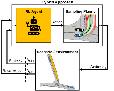
Figure 1: Hybrid reinforcement learning principle of a motion planning agent. The agent’s action informs an analytical (e.g., sampling-based) method to achieve the goal.

In contrast, hybrid methods combining analytical and machine learning models are expected to offer advantages in both areas. Therefore, we present a new approach to motion planning with a two-stage agent, shown in Fig. 1. In this methodology, the foundational robustness of analytic models is integrated with the dynamic learning capabilities of machine learning algorithms, enhancing both performance and adaptability in driving behavior contexts. This hybrid approach effectively bridges the gap between theoretical constructs and practical application, particularly in environments with complex, non-linear data patterns. Notably, these hybrid models often require less data for effective training, providing an advantage in data-poor scenarios [3, 9, 10, 11]. Furthermore, the efficient integration of safety methods and additional functionalities into the analytical planning algorithm is possible. In summary, this work presents three main contributions:

1. A Hybrid motion planning methodology: This encompasses the creation of a motion planning approach that integrates environment and prediction information within a Frenet coordinate system. The focus is on leveraging the strengths of the hybrid model to improve motion planning capabilities.

2. Performance analysis: The new methodology will undergo extensive analysis to assess its efficiency, effectiveness, and improvement areas, providing valuable insights into the hybrid model approach’s performance across different scenarios.

3. Open-source software: An executable software framework will be available as open-source to integrate additional approaches.

II Related work

Autonomous driving motion planning has been an area of intense research for many years. Several approaches are being developed to address the planning task of autonomous driving. Planning methods can be divided into the following categories at a high level [12, 9, 3, 13]: Graph-based algorithms navigate through networks of nodes and edges to find structured paths [12, 3, 14]. Sampling-based methods explore a wide range of trajectories by generating numerous possibilities [15, 16, 17, 18]. Optimization-based planning methods aim to find the most effective trajectory by systematically evaluating various constraints and objectives, often using techniques like linear programming, dynamic programming, or gradient-based optimization [12, 3, 19, 20, 21, 22]. Furthermore, algorithms that utilize artificial intelligence are developed to provide high adaptability in dynamic environments, demonstrating the integration of adaptive computational techniques in this domain [12, 3, 9, 23, 6]. There are several machine learning models in the literature that learn to control the steering wheel and acceleration. These models are almost exclusively trained using specific scenarios such as highway driving or decision-making agents [4, 24, 25, 26, 27, 28]. Although the models show improvement, the success rate for more difficult scenarios is too low, especially for real-world application [4]. Learning human-like behavior is also investigated through inverse RL [29, 30]. The driving behavior of certain characteristics can be learned and adopted. However, this does not lead to a fundamentally higher success rate. The contribution of Xiao et al. [11, 10] explores how iterative learning and human feedback can improve navigation in complex environments for autonomous robots. By integrating these elements into traditional navigation systems, the study demonstrates potential performance improvements while keeping the systems safe and interpretable. This research offers a notable perspective on developing adaptive navigation systems in robotics. The results, while promising, primarily serve as a proof of concept. They do not incorporate complex public road environments or account for the prediction uncertainties of other road users. Moreover, the approach does not integrate a complex analytical planning algorithm; instead, it relies on machine learning to assimilate parameter settings based on expert knowledge. Yu et al. [31] present a framework combining RL with a rapidly exploring random tree for autonomous vehicle motion planning. It focuses on efficiently controlling vehicle speed and ensuring safety, using deep learning techniques to adapt to varying traffic conditions. The primary issue with the approach is its slow convergence rate in high-dimensional state spaces, which compromises its real-time applicability. Furthermore, the method is designed for only certain scenarios, limiting its generalizability. Other research employs RL to determine optimal switching points for executing movements through an analytical model. This approach is applied in scenarios such as timing lane changes and facilitating interaction behaviors among different road users [32, 33, 28]. The current scientific landscape shows a gap in exploring a hybrid approach that combines machine learning with a powerful analytical algorithm for trajectory planning that ensures high success rates, real-time capability, interpretability, and the integration of additional safety features. Strengths and weaknesses could be investigated with such a concept independent of supervised learning datasets.

III Methodology

This section presents the combination of the analytical sampling-based trajectory planner architecture and the RL design for developing the hybrid motion planning method.

III-A Sampling-based Motion Planner

The analytical trajectory planning algorithm used is a sampling-based approach in the Frenet coordinate system according to the concept of Werling et al. [15, 16]. The software is online and available on GitHub. We use a neural network-based algorithm to predict other vehicles in the scenario [34]. The procedure of the algorithm during one timestep is shown in Fig. 2.

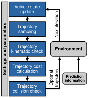
Figure 2: Frenetix Motion Planner: sampling-based motion planning procedure for one timestep including prediction information and environment state update.

The procedure can be summarised into the following main stages:

• Vehicle state update: The vehicle updates all states concerning the Frenet coordinate system using the ego, prediction, and environment information.

• Trajectory sampling: The algorithm samples possible trajectories regarding a sampling matrix. We use time-, velocity-, and lateral-sampling metrics to create different trajectory schemes dependent on the current ego vehicle state [15, 16].

• Trajectory kinematic check: The generated trajectories are checked for kinematic feasibility as a function of a single-track model and the vehicle parameters.

• Trajectory cost calculation: We use different cost metrics like collision probability, jerk, distance to reference path, and velocity offset costs to differentiate between the performance of different trajectories. We integrate the collision probability cost with other obstacles from the prediction information [34]. The trajectory generation is implemented in C++ to reduce calculation time and accelerate the training process.

• Trajectory collision check: The lowest cost trajectory is analyzed for possible collisions with the lane boundary and other obstacles [35]. This step takes place after the cost calculation step for computational efficiency. The first collision-free trajectory sorted by absolute cost is the optimal trajectory to update the current vehicle state.

The vehicle’s status is updated based on the optimal trajectory calculated for each successive timestep. The trajectories encompass a horizon of $3\text{\,}\mathrm{s}$. The timestep discretization of the simulation $0.1\text{\,}\mathrm{s}$.

III-B Reinforcement Learning Procedure

In this section, we are integrating an RL algorithm, which optimizes the trajectory selection process for the presented sampling-based trajectory planner of Section III-A. For the customized environment and training process, we use gymnasium and stable-baselines3. For the agent’s simulation environment, we utilize CommonRoad [36, 4]. The optimization is performed by Proximal Policy Optimization (PPO) [37], an RL algorithm that balances exploration and exploitation by clipping the policy update. It avoids large policy updates that could collapse performance, making training more stable and reliable. The core of the PPO algorithm is encapsulated in Eq. 1 [37]:

$$L^{CLIP}(\theta) =\hat{\mathbb{E}}_{t}\left[\min(r_{t}(\theta)\hat{A}_{t},\right.$$

$$\quad\left.\text{clip}(r_{t}(\theta),1-\epsilon,1+\epsilon)\hat{A}_{t})\right]$$ (1)

This equation represents the clipped surrogate objective function, which is crucial for the efficiency and stability of the PPO algorithm. Here, $\theta$ represents the policy parameters, $\hat{\mathbb{E}}_{t}$ is the empirical expectation over timesteps, $r_{t}(\theta)$ signifies the probability ratio under new versus old policies, $\hat{A}_{t}$ denotes the estimated advantage at time $t$, and $\epsilon$ is a critical hyperparameter controlling the clipping in the objective function. We use Recurrent PPO Optimization with MlpLstmPolicy to process temporal relationships and information. The conventional PPO architecture is extended with Long Short-Term Memory (LSTM) networks [38], a recurrent neural network suited for dynamic, time-series data. This approach is effective in sequential data and partially observable environments. The LSTM component can be formulated as follows:

• LSTM state update: At each timestep $t$, the LSTM updates its hidden state $h_{t-1}$ and cell state $c_{t}$ based on the current input $x_{t}$, previous hidden state $h_{t-1}$, and previous cell state $c_{t-1}$. Expressed as: $(h_{t},c_{t})=LSTM(x_{t},h_{t-1},c_{t-1})$

• Policy and value function: The updated hidden state $h_{t}$ is then utilized by the policy network $\pi(a_{t}|s_{t},h_{t})$ and the value network $V(s_{t},h_{t})$, where $a_{t}$ is the action and $s_{t}$ is the state at time $t$. This integration enables the network to remember past states, enhancing decision-making in complex environments.

In order to initiate the optimization process, it is necessary to first design several key components: the observational space, the criteria for termination, the structure of the reward system, and the definition of the agent’s action space. Fig. 3 shows a class diagram that provides an overview of the functions integral to the training procedure.

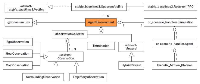
Figure 3: Class diagram of the learning process structure.

Observation space: The observation space is divided into the categories and observations in Section III-B.

TABLE I: Observation space of the learning process.

Categories	Observations
Ego	Velocity, acceleration, jerk, steering, orientation, yaw, distance to reference path
Goal	Distance to goal, remaining time, goal reached, timeout, target velocity
Surrounding	Adjacent lanes, the direction of adjacent lanes, obstacle information
Trajectory	Percentage of feasible trajectories, validity of trajectories, ego risk, obstacle (3-party) risk
Cost	Cost of optimal trajectory, cost mean & variance of all trajectories, cost collision probability

The categories can be segmented into various types: those originating from the ego vehicle, those pertinent to achieving the goal region, surrounding information, trajectory details, and cost information related to the sampled trajectories. Unlike other systems that merely assume direct vehicle control [4], our methodology provides supplementary data that enhances the observation space. The several hundred sampled trajectories of the trajectory planning algorithm contain additional information through the calculation steps in Fig. 2. Key elements of this data include the count of kinematically feasible trajectories, the associated risk level of each trajectory, and their respective cost distributions. Furthermore, we use our concept, depicted in Fig. 4, to address collision probability perception.

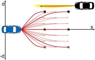
Figure 4: Trajectory cost observation space. The cost calculations of the outermost trajectories perceive additional cost information at each timestep.

The schematic illustration presents the sampled trajectories. We can construct a grid by employing time-, speed-, and lateral-dependent sampling. This grid allows us to analyze the variation in collision probability costs associated with the outermost trajectories, enriching the observation space. Such an approach enables the mapping of differences and correlations over time. In the illustration, trajectories in the positive lateral d-direction are attributed to higher collision probability costs than those in the negative d-direction.

Action space: Fig. 1 shows the connection between the analytical trajectory planner and the RL agent. The agent learns the action, which is the cost weight of the trajectory planner. Theoretically, any adjustment can be passed to the trajectory planner. In our case, we investigate the adjustment of cost weights to prove the concept. To achieve a harmonic behavior, the agent can reduce or increase the current cost weights of the trajectory planner. Eq. 2 shows the action space of the agent regarding each cost term $i$ in timestep $t$.

$$\omega_{i}^{t}=\omega_{i}^{\text{min}}\leq\omega_{i}^{prev}+\omega_{i}^{action}\leq\omega_{i}^{\text{max}}$$ (2)

Consider $\omega_{i}^{\text{action}}$, a floating-point value in the range $[a_{\text{min}},a_{\text{max}}]$. Here, $\omega_{i}^{\text{min}}$ and $\omega_{i}^{\text{max}}$ represent the predefined minimum and maximum values of the absolute cost term, respectively. Additionally, $\omega_{i}^{prev}$ denotes the weight from the previous timestep, while $\omega_{i}^{action}$ signifies the current action of the algorithm. It is important to note that after each execution, the cost terms are reset to their default values.

Reward design: The training process requires the reward configuration and is crucial for success and driving behavior. The rewards we use for the learning process are shown in Table II:

TABLE II: Hybrid Reward of the PPO Training Process.

Sparse reward	Dense reward
Goal reached	Distance to reference path
Goal reached (faster than target time)	Difference to target velocity
Goal reached (slower than target time)	S-distance to goal
Collision	Standard cost difference
No feasible solution	Ego risk
Scenario timeout	Obstacle risk

Our approach uses a hybrid reward system to enhance training efficiency: termination reward and sparse reward. The termination reward is crucial for finishing scenarios successfully, while a sparse reward guides vehicle behavior. The main goal is to minimize collisions, especially influenced by the termination reward. In addition, sparse rewards are required to optimize driving performance and behavior, such as satisfying comfort metrics or minimizing overall driving risk. The vehicle can finalize a scenario in six distinct ways. Each scenario has a distinct time horizon, establishing a window within which the goal can be achieved. This allows for reaching the goal either more quickly or slowly than the allotted time interval, depending on the vehicle’s performance [36]. Scenarios may end due to a collision with obstacles or road boundaries or if the vehicle fails to find a valid trajectory at any timestep. Additionally, if the vehicle stops without reaching the goal, the scenario will automatically terminate after exceeding a specific time limit. The optimal performance involves closely adhering to the reference path, maintaining the designated speed, maximizing progress towards the target distance, and minimizing risk [39, 40]. We are integrating a cost regulation term to enhance stability in the vehicle’s actions. This addition aims to prevent excessive fluctuations in actions, promoting smoother and more harmonious driving behavior. We use the absolute difference between the current action and the default cost settings of the trajectory planner.

IV Results & Analysis

This section shows the model’s training, selected testing scenarios, and results. We will explore the model qualitatively and quantitatively, highlighting the practicality of the concept. We will investigate the differences between the standalone default analytical trajectory planner (DP) and the proposed hybrid planner (HP).

IV-A Environment and Training Setup

We use T-junction scenarios (see Fig. 6) for the training process as they exhibit complex and critical interaction dynamics with other vehicles [36]. Various scenarios in the data set offer a certain degree of variability to reduce the risk of overfitting. For the training and execution of the model, the computational resources include an AMD 7950x processor, an NVIDIA GeForce RTX 4090 graphics card, and 128GB of RAM. The hyperparameters used in our study are shown in Table III.

TABLE III: Hyperparameters of the PPO Algorithm.

Hyperparameter	Value
Learning Rate	$0.0003\text{\,}$
Clipping parameter $\epsilon$	$0.1\text{\,}$
Discount factor $\gamma$	$0.99\text{\,}$
GAE $\lambda$	$0.97\text{\,}$
Batch Size	$2352\text{\,}$
Epochs	$5\text{\,}$
Entropy coefficient	$0.01\text{\,}$

The training is parallelized to the number of cores and requires approximately $24\text{\,}\mathrm{h}$ for $7\text{\,}$ million timesteps. The data is classified into training set ($75\text{\,}\mathrm{\char 37\relax}$), validation set ($15\text{\,}\mathrm{\char 37\relax}$), and test set ($10\text{\,}\mathrm{\char 37\relax}$). The best model is selected based on the reward function in a series of evaluation scenarios. The training converges after $2\text{\,}$-$3\text{\,}$ million training steps, depending on the settings. We use hyperparameter tuning because the training results are highly dependent on it.

IV-B Risk-aware Trajectory Planning

First, we look at the risk behavior of the learned agent, for which we also set a reward (see Table II) to optimize the agent’s behavior. In addition to the success rate, the risk in autonomous driving is also decisive in evaluating the safety of the algorithm. The risk is subsequently calculated by multiplying the maximum collision probability $p$ of a trajectory $\mathcal{T}$ by the harm $H$ incurred [39, 41, 40].

$$\begin{split}R(\mathcal{T})=\mathrm{max}(p(\mathcal{T})H(\mathcal{T}))\end{split}$$ (3)

Our evaluation encompasses $64\text{\,}$ distinct scenarios to assess risk levels. We gain valuable insights into the overall safety landscape by calculating the mean risk across all scenarios. Notably, the results indicate a reduced risk for the ego vehicle and 3-party road users, highlighting improved road safety. Fig. 5 shows the ego-vehicle risk of the scenarios and the 3-party risks. Blue indicates the HP and orange is the DP. The HP shows only about $33\text{\,}\mathrm{\char 37\relax}$ of the risk for the ego vehicle compared to the DP.

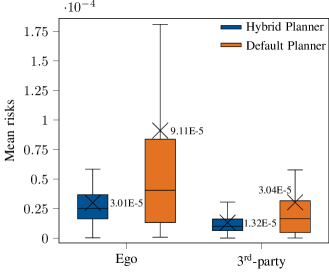
Figure 5: Mean ego and 3-party risks over various scenarios according to [39]. Blue indicates the HP, and orange the DP.

The agent’s reward for reducing the risk has a sustainable influence on the selection process of the trajectories. Our analysis demonstrates that, despite the complexity of numerous target variables, the vehicle can modify its behavior. It is crucial to emphasize the importance of carefully selecting reward terms within this framework. An overly aggressive pursuit of risk reduction through reward mechanisms may lead to scenarios where the vehicle opts to halt completely in certain situations. To mitigate this, we have incorporated a specific reward term, as delineated in Table II, which ensures adherence to the designated target speed, thereby balancing safety with operational efficiency in a controlled manner. The risk is calculated based on the selected trajectory and depends on the planning horizon. The DP accepts a significantly higher risk for a short period and only reacts to the reduction once the risk has been recognized. On the other hand, the model presented here recognizes risky situations before they occur through environmental and obstacle information. The risk is significantly reduced both in absolute terms and in terms of its duration. By slowing down in advance, it can also be determined that the risk peaks occur with a time delay to the risk peaks of the DP.

IV-C Adaption of the Agent’s Driving Behavior

The HP makes it possible to adapt the driving behavior of the analytic trajectory planning algorithm during runtime. In the following analysis, we show the differences in driving behavior between the proposed model and the standalone analytical trajectory planner. Fig. 6 illustrates the HP compared to the DP in the same scenario in blue and orange, respectively.

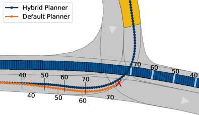
Figure 6: Turning left with HP (blue) and DP (orange) with oncoming traffic. Illustrated with time progression by timestamps. The collision of the DP is marked with a red cross.

Qualitatively, a strong adaptation of the driving behavior due to the oncoming vehicle can be determined. The center positions of the ego vehicle are shown according to the timestamp points. As the blue trajectory indicates, our methodology demonstrates improved adherence to the designated reference path, complemented by earlier braking initiation. In contrast, the DP drives with a greater deviation from the reference path but quickly approaches the oncoming vehicle.

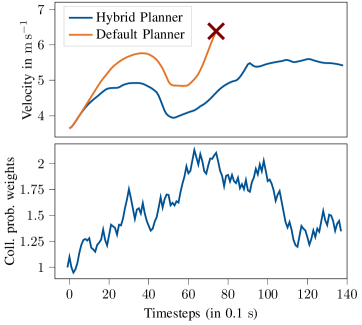
Figure 7: Velocity profile of the HP and the DP and the relative changes in the collision probability weights due to the actions of the hybrid planner. The collision of the DP is marked with a red cross.

This accelerated approach results in an unintended violation of the vehicle’s safety limits at the 74 timestep, which leads to a collision with the oncoming vehicle. The scenario can be completed by carefully changing the manually set parameters of the DP. However, the results show that our HP can avoid manually tuning the parameters. Fig. 7 shows the velocity of the DP and HP and the HP agent’s actions to adjust the planner’s collision probability weights during the same scenario. The velocity of the HP is significantly reduced compared to the DP so that no collision can occur in this situation. This is achieved by successively increasing the weights for the collision probability cost term through the agent’s actions. The RL model can even partially compensate for conceptual errors in the cost function, which can be derived from the strong acceleration of the DP in this situation.

The active ego risk reduction during a scenario can be illustrated in Fig. 8. It can be seen that the sum at risk is significantly lower in our model. The theoretically calculated risk does not necessarily reflect the occurrence of a collision. However, the collisions are avoided by the model, and the risk, which is calculated with the potential harm, is minimized. Incorrect predictions of the objects cause the actions that lead to a collision of the DP. The results show that these can be compensated through the model.

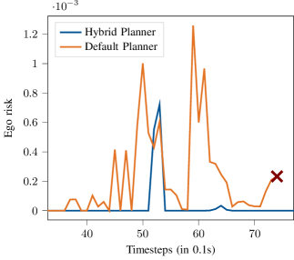
Figure 8: Ego vehicle risk distribution of the HP and DP algorithms [41, 40]. Risk is plotted over a specific time interval, with each step representing $0.1\text{\,}\mathrm{s}$. The collision of the DP is marked with a red cross.

IV-D Scenario Performance Evaluation

The next study evaluates the success rates of our method. Different cost parameters for collision probability are applied in the DP to ensure parameterization accuracy. The results are compared with the HP, as shown in Fig. 9.

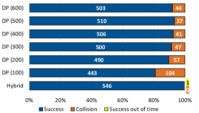
Figure 9: Comparison of the DP and the HP with $547\text{\,}$ scenarios. The DP is executed with different collision probability costs to investigate different setups. Orange indicates the number of scenarios with collisions.

It can be noted that the DP has a high success rate but has collisions in every configuration. The appropriate setting of collision probability costs is crucial to balance the algorithm. Costs set too low may lead to collisions from excessively aggressive driving. Conversely, excessively high costs might result in rear-end collisions due to overly cautious behavior. The DP lacks sufficient flexibility and requires further features for optimal performance. The trained HP performs exceptionally, with no collisions observed, even in previously unseen test scenarios. Differences in driving behavior can be obtained from Table IV.

TABLE IV: Driving characteristic measurements between the default and hybrid planner over various scenarios.

	Measurements	Max	Average	Median	$\sigma$
Default	d-position in $\text{\,}\mathrm{m}$	$0.251\text{\,}$	$-0.102\text{\,}$	$-0.0188\text{\,}$	$0.22\text{\,}$
	Velocity in $\text{\,}\mathrm{m}\text{\,}{\mathrm{s}}^{-1}$	$9.784\text{\,}$	$6.786\text{\,}$	$6.77\text{\,}$	$0.986\text{\,}$
	Cost unweighted	$578.87\text{\,}$	$17.895\text{\,}$	$3.07\text{\,}$	34.07
Hybrid	d-position in $\text{\,}\mathrm{m}$	0.726	$-0.11\text{\,}$	$-0.0126\text{\,}$	$0.224\text{\,}$
	Velocity in $\text{\,}\mathrm{m}\text{\,}{\mathrm{s}}^{-1}$	8.179	$5.98\text{\,}$	$6.132\text{\,}$	$0.9897\text{\,}$
	Cost unweighted	$2024\text{\,}$	$20.07\text{\,}$	$1.11\text{\,}$	78.72

The HP exhibits enhanced adaptability regarding the maximum permissible deviation from the reference path. In addition, the maximum and average velocity is reduced to improve the turning maneuver for the T-junction scenarios. Furthermore, the costs associated with the optimal trajectory in the HP show a more substantial deviation. This increased deviation is feasible due to the application of variable weights, offering a more nuanced approach to trajectory optimization.

IV-E Execution Time Evaluation

Fig. 10 illustrates the execution time per iteration in $\text{\,}\mathrm{s}$ for three critical components within the RL framework in the box-plot format: the RL model prediction execution, the sampling step of the DP, and the overall model execution.

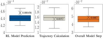
Figure 10: Execution time per iteration of the RL model prediction, the trajectory bundle calculations, and the overall model in $\text{\,}\mathrm{s}$.

The calculation time is determined based on ten different scenarios. The average for the execution of agent prediction is approximately $0.44\text{\,}\mathrm{ms}$. This step only includes the execution of the neural network and not the update of the environment model. An average of around $15.8\text{\,}\mathrm{ms}$ is required for the generation, validity check, and cost calculation of around $800\text{\,}$ trajectories per timestep. Increasing the number of trajectories in the analytical planning step has little impact on the computation time because the parallelized process is stable due to the C++ package extension. Running the entire model requires an average execution time of about $46\text{\,}\mathrm{ms}$ per iteration.

V Discussion

The results show that the hybrid approach is effective and can significantly improve the analytical model with low execution times. In contrast to other pure RL models, the training process is fast and the model has a high success rate [4, 6, 9]. The generalisability increases significantly. Although the purely analytical model performs comparatively well in certain situations, performance can vary from situation to situation. In addition, with the right setup, the proposed model can compensate for the errors of other models, such as the prediction algorithm. However, substantial alterations to the algorithm necessitate a partial retraining of the agent model. The design of the method can also be adapted and enhanced. Thus, the limits from Eq. 2 are frequently exploited, which indicates that the model can be improved. In addition, the choice of reward values and scenarios must be carefully considered, which can be time-consuming. Overall, our concept demonstrates the effective use of the synergies offered by the hybrid planner and extends the currently available methods through greater complexity and applicability in edge-case scenarios [28, 31, 33].

VI Conclusion & Outlook

This paper introduces a hybrid motion planner approach for trajectory planning to enhance vehicle driving behavior under changing conditions. Addressing the low generalizability of traditional analytical trajectory planners, our method combines a sampling-based planner with an RL agent. This agent dynamically adjusts the cost weights in the analytical algorithm, boosting its adaptability. Our approach utilizes an observation space, including the environmental, semantic map, and obstacle data, which are crucial for the hybrid agent’s learning about vehicle dynamics. The results show a significant improvement in the agent’s success rate and a reduction in risk while maintaining high-performance execution times for real-world applications. Nevertheless, additional features could improve driving behavior and model performance through more extensive investigations. Future work could optimize the sampling parameters of the analytical planner using RL and thus investigate the algorithm’s applicability in the real world. Including more comprehensive environmental data, e.g., through graph representations, could further increase the stability and efficiency of the system.

References

- [1] California Department of Motor Vehicles, “Autonomous vehicle collision reports,” 2023, accessed: December 20, 2023. [Online]. Available: https://www.dmv.ca.gov/portal/vehicle-industry-services/autonomous-vehicles/autonomous-vehicle-collision-reports/
- [2] S. Aradi, “Survey of deep reinforcement learning for motion planning of autonomous vehicles,” IEEE Transactions on Intelligent Transportation Systems, vol. 23, no. 2, pp. 740–759, 2022.
- [3] C. Zhou, B. Huang, and P. Fränti, “A review of motion planning algorithms for intelligent robots,” Journal of Intelligent Manufacturing, vol. 33, no. 2, pp. 387–424, 2022.
- [4] X. Wang, H. Krasowski, and M. Althoff, “Commonroad-rl: A configurable reinforcement learning environment for motion planning of autonomous vehicles,” in 2021 IEEE International Intelligent Transportation Systems Conference (ITSC), 2021, pp. 466–472.
- [5] J. Dinneweth, A. Boubezoul, R. Mandiau, and S. Espié, “Multi-agent reinforcement learning for autonomous vehicles: a survey,” Autonomous Intelligent Systems, vol. 2, no. 1, p. 27, 2022.
- [6] S. Shalev-Shwartz, S. Shammah, and A. Shashua, “Safe, multi-agent, reinforcement learning for autonomous driving,” 2016.
- [7] D. Minh, H. X. Wang, Y. F. Li, and T. N. Nguyen, “Explainable artificial intelligence: a comprehensive review,” Artificial Intelligence Review, vol. 55, no. 5, pp. 3503–3568, 2022.
- [8] A. Arrieta and et al., “Explainable artificial intelligence (xai): Concepts, taxonomies, opportunities and challenges toward responsible ai,” Information Fusion, vol. 58, pp. 82–115, 2020.
- [9] L. Dong, Z. He, C. Song, and C. Sun, “A review of mobile robot motion planning methods: from classical motion planning workflows to reinforcement learning-based architectures,” Journal of Systems Engineering and Electronics, vol. 34, no. 2, pp. 439–459, 2023.
- [10] X. Xiao, B. Liu, G. Warnell, and P. Stone, “Motion planning and control for mobile robot navigation using machine learning: a survey,” Autonomous Robots, vol. 46, no. 5, pp. 569–597, 2022.
- [11] X. Xiao and et al., “Appl: Adaptive planner parameter learning,” Robotics and Autonomous Systems, vol. 154, p. 104132, 2022.
- [12] S. Teng and et al., “Motion planning for autonomous driving: The state of the art and future perspectives,” IEEE Transactions on Intelligent Vehicles, vol. 8, no. 6, pp. 3692–3711, 2023.
- [13] B. Paden, M. Čáp, S. Z. Yong, D. Yershov, and E. Frazzoli, “A survey of motion planning and control techniques for self-driving urban vehicles,” IEEE Transactions on Intelligent Vehicles, vol. 1, no. 1, pp. 33–55, 2016.
- [14] M. Rowold, L. Ögretmen, T. Kerbl, and B. Lohmann, “Efficient spatiotemporal graph search for local trajectory planning on oval race tracks,” Actuators, vol. 11, no. 11, 2022.
- [15] M. Werling, J. Ziegler, S. Kammel, and S. Thrun, “Optimal trajectory generation for dynamic street scenarios in a frenét frame,” in 2010 IEEE International Conference on Robotics and Automation. IEEE, 2010, pp. 987–993.
- [16] M. Werling, S. Kammel, J. Ziegler, and L. Gröll, “Optimal trajectories for time-critical street scenarios using discretized terminal manifolds,” The International Journal of Robotics Research, vol. 31, no. 3, pp. 346–359, 2012.
- [17] J. Huang, Z. He, Y. Arakawa, and B. Dawton, “Trajectory planning in frenet frame via multi-objective optimization,” IEEE Access, vol. 11, pp. 70 764–70 777, 2023.
- [18] G. Würsching and M. Althoff, “Sampling-based optimal trajectory generation for autonomous vehicles using reachable sets,” in 2021 IEEE International Intelligent Transportation Systems Conference (ITSC), 2021, pp. 828–835.
- [19] Y. Cao, W. ShangGuan, B. Cai, L. Chai, and W. Qiu, “Predictive trajectory planning for on-road autonomous vehicles based on a spatiotemporal risk field,” IEEE Intelligent Transportation Systems Magazine, vol. 15, no. 1, pp. 400–420, 2023.
- [20] Y. Li, “Motion planning for dynamic scenario vehicles in autonomous-driving simulations,” IEEE Access, vol. 11, pp. 2035–2047, 2023.
- [21] D. Jeong and S. B. Choi, “Efficient trajectory planning for autonomous vehicles using quadratic programming with weak duality,” IEEE Transactions on Intelligent Vehicles, pp. 1–15, 2023.
- [22] J. Zhu, X. Qi, Y. Zhao, B. Lian, Y. Dong, and X. Wang, “Fast trajectory path planning inspired by binary searching algorithm,” in 2023 IEEE International Conference on Mechatronics and Automation (ICMA), 2023, pp. 2265–2271.
- [23] B. B. Elallid, N. Benamar, A. S. Hafid, T. Rachidi, and N. Mrani, “A comprehensive survey on the application of deep and reinforcement learning approaches in autonomous driving,” Journal of King Saud University - Computer and Information Sciences, vol. 34, no. 9, pp. 7366–7390, 2022.
- [24] B. Mirchevska, M. Werling, and J. Boedecker, “Optimizing trajectories for highway driving with offline reinforcement learning,” Frontiers in Future Transportation, vol. 4, p. 1076439, 2023.
- [25] L. Zhang, R. Zhang, T. Wu, R. Weng, M. Han, and Y. Zhao, “Safe reinforcement learning with stability guarantee for motion planning of autonomous vehicles,” IEEE Transactions on Neural Networks and Learning Systems, vol. 32, no. 12, pp. 5435–5444, 2021.
- [26] M. Al-Sharman, R. Dempster, M. A. Daoud, M. Nasr, D. Rayside, and W. Melek, “Self-learned autonomous driving at unsignalized intersections: A hierarchical reinforced learning approach for feasible decision-making,” IEEE Transactions on Intelligent Transportation Systems, vol. 24, no. 11, pp. 12 345–12 356, 2023.
- [27] Z. Gu, L. Gao, H. Ma, S. E. Li, S. Zheng, W. Jing, and J. Chen, “Safe-state enhancement method for autonomous driving via direct hierarchical reinforcement learning,” IEEE Transactions on Intelligent Transportation Systems, vol. 24, no. 9, pp. 9966–9983, 2023.
- [28] M. Klimke, B. Völz, and M. Buchholz, “Integration of reinforcement learning based behavior planning with sampling based motion planning for automated driving,” in 2023 IEEE Intelligent Vehicles Symposium (IV), 2023, pp. 1–8.
- [29] Z. Huang, H. Liu, J. Wu, and C. Lv, “Conditional predictive behavior planning with inverse reinforcement learning for human-like autonomous driving,” IEEE Transactions on Intelligent Transportation Systems, vol. 24, no. 7, pp. 7244–7258, 2023.
- [30] R. Trauth, M. Kaufeld, M. Geisslinger, and J. Betz, “Learning and adapting behavior of autonomous vehicles through inverse reinforcement learning,” in 2023 IEEE Intelligent Vehicles Symposium (IV), 2023, pp. 1–8.
- [31] J. Yu, A. Arab, J. Yi, X. Pei, and X. Guo, “Hierarchical framework integrating rapidly-exploring random tree with deep reinforcement learning for autonomous vehicle,” Applied Intelligence, vol. 53, no. 13, pp. 16 473–16 486, 2023.
- [32] N. Albarella, D. G. Lui, A. Petrillo, and S. Santini, “A hybrid deep reinforcement learning and optimal control architecture for autonomous highway driving,” Energies, vol. 16, no. 8, 2023.
- [33] R. Jafari, A. E. Ashari, and M. Huber, “Champ: Integrated logic with reinforcement learning for hybrid decision making for autonomous vehicle planning,” in 2023 American Control Conference (ACC), 2023, pp. 3310–3315.
- [34] M. Geisslinger, P. Karle, J. Betz, and M. Lienkamp, “Watch-and-learn-net: Self-supervised online learning for probabilistic vehicle trajectory prediction,” in 2021 IEEE International Conference on Systems, Man, and Cybernetics (SMC). IEEE, 2021.
- [35] C. Pek, V. Rusinov, S. Manzinger, M. Can Üste, and M. Althoff, “Commonroad drivability checker: Simplifying the development and validation of motion planning algorithms,” in Proc. of the IEEE Intelligent Vehicles Symposium, 2020, pp. 1–8.
- [36] M. Althoff, M. Koschi, and S. Manzinger, “Commonroad: Composable benchmarks for motion planning on roads,” in 2017 IEEE Intelligent Vehicles Symposium (IV), 2017, pp. 719–726.
- [37] J. Schulman, F. Wolski, P. Dhariwal, A. Radford, and O. Klimov, “Proximal policy optimization algorithms,” arXiv preprint arXiv:1707.06347, 2017.
- [38] S. Hochreiter and J. Schmidhuber, “Long Short-Term Memory,” Neural Computation, vol. 9, no. 8, pp. 1735–1780, 11 1997.
- [39] M. Geisslinger, F. Poszler, J. Betz, C. Lütge, and M. Lienkamp, “Autonomous driving ethics: from trolley problem to ethics of risk,” Philosophy and Technology, 2021.
- [40] M. Geisslinger, R. Trauth, G. Kaljavesi, and M. Lienkamp, “Maximum acceptable risk as criterion for decision-making in autonomous vehicle trajectory planning,” IEEE Open Journal of Intelligent Transportation Systems, vol. 4, pp. 570–579, 2023.
- [41] M. Geisslinger, F. Poszler, and M. Lienkamp, “An ethical trajectory planning algorithm for autonomous vehicles,” Nat Mach Intell, 2023.