Deep Conditional Generative Learning: Model and Error Analysis

Jinyuan Chang
School of Statistics, Southwestern University of Finance and Economics
Chengdu, 611130, People’s Republic of China
changjinyuan@swufe.edu.cn
&Zhao Ding
School of Mathematics and Statistics, Wuhan University
Wuhan, 430072, People’s Republic of China
zd1998@whu.edu.cn &Yuling Jiao
School of Mathematics and Statistics Hubei Key Laboratory of Computational Science, Wuhan University
Wuhan, People’s Republic of China
yulingjiaomath@whu.edu.cn
&Ruoxuan Li
School of Mathematics and Statistics, Wuhan University
Wuhan, People’s Republic of China
ruoxuanli.math@whu.edu.cn
&Jerry Zhijian Yang
School of Mathematics and Statistics and Hubei Key Laboratory of Computational Science, Wuhan University
Wuhan, People’s Republic of China
zjyang.math@whu.edu.cn
Abstract

We introduce an Ordinary Differential Equation (ODE) based deep generative method for learning a conditional distribution, named the Conditional Föllmer Flow. Starting from a standard Gaussian distribution, the proposed flow could efficiently transform it into the target conditional distribution at time 1. For effective implementation, we discretize the flow with Euler’s method where we estimate the velocity field nonparametrically using a deep neural network. Furthermore, we derive a non-asymptotic convergence rate in the Wasserstein distance between the distribution of the learned samples and the target distribution, providing the first comprehensive end-to-end error analysis for conditional distribution learning via ODE flow. Our numerical experiments showcase its effectiveness across a range of scenarios, from standard nonparametric conditional density estimation problems to more intricate challenges involving image data, illustrating its superiority over various existing conditional density estimation methods.

Keywords Conditional generative model  $\cdot$ ODE flow  $\cdot$ deep neural networks  $\cdot$ End-to-end error bound

1 Introduction

Predicting a response variable $Y$ based on information from a related predictor $X$ is a crucial task in statistics and machine learning. Assuming that $(X,Y)$ is jointly distributed according to $\pi_{1}(\boldsymbol{x},\boldsymbol{y})$, traditional regression models aim to find an appropriate statistical estimator $h(X)$ that effectively approximates $Y$. In certain scenarios, $h(\cdot)$ has an optimal solution $h^{*}(\cdot)$, such as in $L^{2}$ regression where $h^{*}(X)$ represents the conditional mean $\mathbb{E}[Y|X]$, or in $L^{1}$ regression where $h^{*}(X)$ corresponds to the conditional median. Extensive research has focused on the consistency of nonparametric regression estimators under general conditions [1; 2; 3; 4; 5], among others. In addition to establishing consistency, numerous influential works have delved into the analysis of convergence rates for empirical risk minimizers including [6; 7; 8; 9; 10; 11], as well as the monographs [12; 13] and the references therein. Entering the era of deep learning, there has also been significant research on the convergence properties of neural network-based nonparametric regression, such as [14; 15; 16; 17; 18; 19; 20; 21].

However, even if we can achieve the optimality $h^{*}(\cdot)$, which is a point estimation unable to qualify uncertainty nor provide overall distributional information. To illustrate, doctors typically expect to acquire the range of possible values for various medical indicators related to some specific symptom, and prediction intervals are more informative than the prediction itself. Thus, it becomes imperative to learn the conditional distribution, as it reveals the relationship between the response variable and the predictor.

A wealth of classical literature has already delved into nonparametric conditional density estimation, including kernel smoothing and local polynomials [22; 23; 24; 25]; regression reformulation [26; 27]; nearest neighbors [28; 29]; basis function expansion [30; 31; 32] etc. These methods aim to directly estimate the functional form of the conditional density while struggle with high-dimensional data due to the “curse of dimensionality”, where their performance declines as the dimensionality of the dependent variable increases. Indeed, such methods are usually effective for only a few covariates and are designed for scalar responses, lacking the ability to handle high-dimensional responses.

Benefiting from the flourishing advancements in deep generative models, recent years have seen the emergence of novel methods. The GCDS approach [33], inspired by Generative Adversarial Networks (GANs), diverges by concentrating on estimating a conditional sampler rather than the functional form of the conditional density, hence allowing both high-dimensional predictors and responses. Similar applications of GANs can also be found in [34]. However, GANs’ training process tends to be unstable [35], primarily because it is formulated as a minmax problem between the generator and the discriminator.

The recent breakthrough in deep generative models, known as the diffusion model, gains notable attention for its superior sample quality and significantly more stable and controllable training process compared to GANs. The initial concept involves training a denoising model to progressively transform noise data to samples adhering to the target distribution [36], which has soon been proven to mathematically correspond to learning either the drift term of an Stochastic Differential Equation (SDE) or the velocity field of an Ordinary Differential Equation (ODE) [37]. Henceforth, there has been an explosive development in SDE/ODE-based generative models. Basically, in SDE-based methods the target density of data degenerates into some much simpler Gaussian density through Ornstein-Uhlenbeck (OU) process, then a reverse-time SDE is solved to generate samples from noises [36; 37; 38]. Further, researchers propose diffusion Schrödinger Bridge(SB), which formulates a finite time SDE, effectively accelerating simulation time [39]. Regarding the ODE-based methods, the achievements are equally remarkable. The majority of ODE-based methods adopt an approach involving interpolative trajectory modeling [40; 41; 42; 43]. [40] employs linear interpolation to link the target distribution with a reference distribution. [41] extends the interpolation to nonlinear cases. [44] further uses interpolation to analyze the regularity of a large class of ODE flows.

Since the inception of diffusion models, it has been closely associated with the topic of conditional generation, as evidenced by some quite successful applications [45; 46]. With the development of ODE/SDE methods, several applications of conditional generation have also been proposed. For instance, diffusion SB [39] is extended to conditional SB [47]; Also, interpolation methods are applied in conditional scenarios [48]. However, most of these methods essentially require an infinite time horizon, so truncation at a finite time is necessary in practice, introducing additional bias to the final estimation. Meanwhile, there is limited research on the impact of regularity of the drift term or velocity field on the ultimate error of the algorithm.

Recently, [49] introduces the Föllmer Flow, defined over a unit time interval, with well-behaved properties of the velocity field and flow map itself, which aligns well with the scenarios in generative modeling. Furthermore, according to [44], the Föllmer Flow can be viewed as a special case within their theoretical framework.

Inspired by [49; 44], we propose a novel ODE based sampling method named Conditional Föllmer Flow, where the velocity field couples the predictor. More specifically, we formulate the ODE as following, where, in line with the conventions of the generative modeling domain, the predictor is denoted as $Y\in\mathbb{R}^{d_{Y}}$ and the response variable as $X\in\mathbb{R}^{d}$:

$$\mathrm{d}Z(t,\boldsymbol{y})=\boldsymbol{v}_{F}\left(Z(t,\boldsymbol{y}),\boldsymbol{y},t\right)\mathrm{d}t,\ t\in[0,1].$$

For any $\boldsymbol{y}$, $Z(0,\boldsymbol{y})$ is a random variable with dimensions consistent with $X$, following $\pi_{0}=\mathcal{N}\left(0,I_{d}\right)$. After the evolution through $\boldsymbol{v}_{F}$, $Z(1,\boldsymbol{y})$ ought to follow $\pi_{1}(\boldsymbol{x}|\boldsymbol{y})$, which is the distribution of $X|Y=\boldsymbol{y}$. We can then generate $\boldsymbol{z}$ from $\pi_{0}$ and run the ODE dynamics to sample from the conditional distribution:

$$\mathrm{d}Z_{t}=\boldsymbol{v}_{F}\left(Z_{t},\boldsymbol{y},t\right)\mathrm{d}t,\ Z_{0}=\boldsymbol{z}.$$

We estimate $\boldsymbol{v}_{F}$ nonparametrically using neural networks, and use the Euler method to approximate the continuous ODE dynamics.

In the following subsection, we give a quick description of our method.

1.1 Conditional Föllmer Flow and flow based sampling: method description

ODE flows are inherently linked to distribution transformations. Consider a well-posed ODE system: $\mathrm{d}{\boldsymbol{x}}_{t}=\boldsymbol{v}(\boldsymbol{x}_{t},t)\mathrm{d}t$, then for each initial condition $\boldsymbol{x}_{0}\in\mathbb{R}^{d}$, it has a unique solution, which means that starting from any initial point $\boldsymbol{x}_{0}$, through the evolution of the ODE dynamic the system will reach a unique endpoint $\boldsymbol{x}_{t}$ at time $t$. We now define the flow map $\Phi_{t}(\cdot)$ as $\Phi_{t}(\boldsymbol{x}_{0})=\boldsymbol{x}_{t}$. It is evident that, for any given time $t$ , $\Phi_{t}(\cdot)$ determines a mapping from $\mathbb{R}^{d}$ to $\mathbb{R}^{d}$, which maps any initial point to its position at time $t$ under the predefined ODE.

Now, assuming a random variable $X_{0}\in\mathbb{R}^{d}$ and $X_{0}\sim\mu_{0}$, then $X_{t}=\Phi_{t}\left(X_{0}\right)$ defines a new random variable in $\mathbb{R}^{d}$, and its marginal distribution $\mu_{t}$ is entirely determined by $\mu_{0}$ and $\boldsymbol{v}(\boldsymbol{x},t)$. Thus, we achieve distribution transformation through the utilization of the ODE system. Considering conditional distributions, we simply couple information of the predictor into the ODE. Specifically, given $\boldsymbol{y}$ as a realization of the predictor $Y$, i.e. the ‘condition’, the velocity field becomes $\boldsymbol{v}(\boldsymbol{x},\boldsymbol{y},t)$, and the flow map consequently becomes $\Phi_{t}(\cdot,\boldsymbol{y})$. In this way, we can transform $\mu_{0}$ into a distribution $\mu_{t}^{\boldsymbol{y}}$ which depends on $\boldsymbol{y}$. In Section 3, we introduced a meticulously designed velocity field $\boldsymbol{v}_{F}(\boldsymbol{x},\boldsymbol{y},t)\in\mathbb{R}^{d}$, which defines an ODE named Conditional Föllmer Flow, over the unit time interval $[0,1]$. Given $Z_{0}\sim\pi_{0}=\mathcal{N}(0,I_{d})$, we demonstrate that $F_{1}\left(Z_{0},\boldsymbol{y}\right)\sim\pi_{1}(\boldsymbol{x}|\boldsymbol{y})$. More details can be found in Appendix E.1.

Due to the involvement of $\pi_{1}(\boldsymbol{x}|\boldsymbol{y})$ in the definition of $\boldsymbol{v}_{F}$, which is precisely the target we aim to solve, an exact solution for $\boldsymbol{v}_{F}$ is unattainable. Therefore, we opt to utilize a deep neural network $\widehat{\boldsymbol{v}}(\boldsymbol{x},\boldsymbol{y},t)$ to approximate it. By combining Empirical Risk Minimization (ERM) with stochastic gradient descent, we progressively achieve this goal by extracting information from a set of samples $\{(X_{i},Y_{i})\}_{i=1}^{n}$ i.i.d. drawn from the target joint distribution $\pi_{1}(\boldsymbol{x},\boldsymbol{y})$. We concurrently demonstrate that, under appropriate parameterization of the neural network, the error between $\widehat{\boldsymbol{v}}$ and $\boldsymbol{v}_{F}$ converges to zero as the sample size tends to infinity. Relevant conclusions are outlined in Theorem 4 of Appendix C and Proposition 1 of Appendix D.1.

Similar to $F_{t}(\cdot,\boldsymbol{y})$, we use $\widehat{F}_{t}(\cdot,\boldsymbol{y})$ to denote the flow map related to $\widehat{\boldsymbol{v}}(\boldsymbol{x},\boldsymbol{y},t)$. It is evident that obtaining an exact $\widehat{F}_{t}(\cdot,\boldsymbol{y})$ is also infeasible due to the necessity of solving a high-dimensional nonlinear system of ODEs. Consequently, we employ the Euler method to solve the ODE numerically, as described in Section 4.3. This is equivalent to approximating $\widehat{F}_{t}(\cdot,\boldsymbol{y})$ through the composition of a series of mappings $\{\mathcal{T}^{t,N}_{k}(\cdot,\boldsymbol{y})\}_{k=1}^{N}$, i.e.

$\displaystyle\mathcal{T}^{t,N}_{k}(\cdot,\boldsymbol{y})$ $\displaystyle=\mathbb{I}_{d}+\frac{t}{N}\widehat{\boldsymbol{v}}\left(\cdot,\boldsymbol{y},\frac{(k-1)t}{N}\right),\ k=1,\cdots,N,$ (1)
$\displaystyle\widetilde{F}_{t}(\cdot,\boldsymbol{y})$ $\displaystyle=\mathcal{T}^{t,N}_{N}\circ\mathcal{T}^{t,N}_{N-1}\circ\cdots\circ\mathcal{T}^{t,N}_{1}(\cdot,\boldsymbol{y}),$
$\displaystyle\widetilde{F}_{t}(\cdot,\boldsymbol{y})$ $\displaystyle\approx\widehat{F}_{t}(\cdot,\boldsymbol{y}),$

where $\mathbb{I}_{d}$ is the identity map and $N$ is the size of temporal grid. For numerical stability, during sampling we select $t=T<1,T\approx 1$ as the stopping time. In Lemma 5 of Appendix D.2, we meticulously analyze the error between $\widehat{F}_{T}(\cdot,\boldsymbol{y})$ and $\widetilde{F}_{T}(\cdot,\boldsymbol{y})$ under such numerical discretization.

Combining above discussions, we summarize the sampling process based on Conditional Föllmer Flow as follows: First, a deep learning algorithm outputs $\widehat{\boldsymbol{v}}$ as an approximation to the true velocity field ${\boldsymbol{v}}_{F}$. Then, given $\boldsymbol{y}$ as the ‘condition’ and $Z_{0}\sim\pi_{0}$, we choose a stopping time $T<1$, and use the method described in the previous section to obtain $\widetilde{F}_{T}\left(Z_{0},\boldsymbol{y}\right)$ approximately following $\pi_{1}(\boldsymbol{x}|\boldsymbol{y})$. In the main result, Theorem 2, we provide an end-to-end error analysis of our approach, where ‘end-to-end’ refers to a direct analysis of the Wasserstein-2 distance between $\operatorname{Law}(\widetilde{F}_{T}\left(Z_{0},\boldsymbol{y}\right))$ and $\pi_{1}(\boldsymbol{x}|\boldsymbol{y})$. We establish that, with a sufficiently large time steps $N$ and an appropriately chosen stopping time $T$, $W^{2}_{2}\left(\operatorname{Law}(\widetilde{F}_{T}\left(Z_{0},\boldsymbol{y}\right)),\pi_{1}(\boldsymbol{x}|\boldsymbol{y})\right)$ averagely tends to zero with convergence rate $\widetilde{\mathcal{O}}\left(n^{-\frac{4}{9\left(d+d_{Y}+5\right)}}\right)$ as the sample size $n$ approaches infinity. Here, $d$ and $d_{Y}$ respectively represent the dimensions of the response $X$ and predictor $Y$.

It is also worth noting that, we will employ an additional neural network to retain information about the composition map $\widetilde{F}_{T}(\cdot,\boldsymbol{y})$. This approach facilitates one-step generation, significantly reducing model inference time. Our exploration can be found in Section 7.

1.2 Contributions

Our contributions can be summarized in three folds:

  1. (i)

    We propose an ODE system over a unit time interval, and under appropriate assumptions, both the velocity and the flow itself exhibit Lipschitz continuity, mathematically ensuring robustness in both the training and sampling processes. This assures that our method excels in managing high-dimensional responses and accommodates a variety of predictor and response types, encompassing both continuous and discrete variables.

  2. (ii)

    We prove the convergence property of the proposed method, accompanied with a comprehensive end-to-end error analysis, which represents the first study in the field of ODE based conditional distribution learning to our best knowledge.

  3. (iii)

    We conduct a series of numerical experiments using our method and demonstrate its effectiveness in tackling complex data challenges. This is exemplified through tasks such as image generation and reconstruction.

1.3 Organization

The remainder of this paper is structured as follows. In Section 2, we provide notations and introduce the necessary assumptions. In Section 3, we formally introduce the Conditional Föllmer Flow and discuss its well-posedness and associated properties. In Section 4, we present how to approximate the velocity field $\boldsymbol{v}_{F}$ with neural networks and implement the Conditional Föllmer Flow using the Euler method. In Section 5, we analyze the convergence of the numerical scheme under reasonable conditions, and present an end-to-end error analysis. In section 6, we will introduce related work in the fields of conditional generative learning and error analysis in generative models, providing a detailed comparison with our work. Finally, in Section 7, we conduct numerical experiments to demonstrate its performance. Proofs and technical details are provided in the supplementary material.

2 Preliminaries

2.1 Notations

We denote $[N]:=\{0,\cdots,N-1\}$. For matrices $A$ and $B$, we say $A\preceq B$ if $B-A$ is positive semi-definite. The identity matrix in $\mathbb{R}^{d\times d}$ is denoted by $I_{d}$. For a vector $\boldsymbol{x}\in\mathbb{R}^{d}$, we define $\boldsymbol{x}^{\otimes 2}:=\boldsymbol{x}\boldsymbol{x}^{T}$. The $\ell^{2}$-norm of a vector $\boldsymbol{x}$ is denoted by $\|\boldsymbol{x}\|:=\sqrt{\sum_{i=1}^{d}x_{i}^{2}}$ and The $\ell^{\infty}$-norm of a vector $\boldsymbol{x}$ is denoted by $\|\boldsymbol{x}\|_{\infty}:=\max_{i=1}^{d}|x_{i}|$. The operator norm of a matrix $A$ is defined as $\|A\|_{\text{op}}:=\sup_{\|x\|\leq 1}\|Ax\|$. For a twice continuously differentiable function $f:\mathbb{R}^{d}\rightarrow\mathbb{R}$, let $\nabla f$, $\nabla^{2}f$, and $\Delta f$ denote its gradient, Hessian, and Laplacian, respectively. For a probability density function $\pi$ and a measurable function $f:\mathbb{R}^{d}\rightarrow\mathbb{R}$, the $L^{2}(\pi)$-norm of $f$ is defined as $\|f\|_{L^{2}(\pi)}:=\left(\int(f(\boldsymbol{x}))^{2}\pi(\boldsymbol{x})\mathrm{d}\boldsymbol{x}\right)^{1/2}$. The $L^{\infty}(K)$-norm is defined as $\|f\|_{L^{\infty}(K)}:=\sup_{\boldsymbol{x}\in K}|f(\boldsymbol{x})|$. For a vector function $\boldsymbol{v}:\mathbb{R}^{d}\rightarrow\mathbb{R}^{d}$, its $L^{2}(\pi)$-norm is denoted as $\|\boldsymbol{v}\|_{L^{2}(\pi)}:=\|\boldsymbol{v}\|_{L^{2}(\pi)}$, and the $L^{\infty}(K)$-norm is denoted as $\|\boldsymbol{v}\|_{L^{\infty}(K)}:=\|\boldsymbol{v}\|_{L^{\infty}(K)}$. We use $U(a,b)$ to denote the uniform distribution on interval $(a,b)$, and use $\mathcal{N}(0,I_{d})$ to denote the $d$-dimensional standard normal distribution. The asymptotic notation $f(x)=\mathcal{O}(g(x))$ denotes $f(x)\leq Cg(x)$ for some constant $C>0$. The notation $\widetilde{\mathcal{O}}(\cdot)$ is used to ignore logarithmic terms. Given two distributions $\mu$ and $\nu$, the Wasserstein-2 distance is defined as $W_{2}(\mu,\nu):=\inf_{\pi\in\Pi(\mu,\nu)}\mathbb{E}_{(x,y)\sim\pi}[\|x-y\|^{2}]^{1/2}$, where $\Pi(\mu,\nu)$ is the set of all couplings of $\mu$ and $\nu$. A coupling is a joint distribution on $\mathbb{R}^{d}\times\mathbb{R}^{d}$ whose marginals are $\mu$ and $\nu$ on the first and second factors, respectively.

2.2 Assumptions

We address four assumptions under which we will build the Conditional Föllmer Flow.

Remark 1

From now on, we will use $X_{1}$ to represent the response variable in this paper, replacing the previous notation $X$.

Assumption 1 (Bounded predictor)

The predictor $Y$ takes value in $[0,B_{Y}]^{d_{Y}}$, where $B_{Y}\in(0,+\infty)$.

Assumption 2 (Bounded response)

$\pi_{1}(\boldsymbol{x}|\boldsymbol{y})=\operatorname{Law}(X_{1}|Y=\boldsymbol{y})$ is supported on $[0,1]^{d}$ for any $\boldsymbol{y}\in[0,B_{Y}]^{d_{Y}}$.

Remark 2

Boundedness of predictors is a classical assumption in density estimation [50]. As for the response variable, its natural boundedness is evident in classification problems. In regression, the boundedness of the response variable implies bounded noise, an assumption that can be removed through suitable truncation argument [13].

Assumption 3 (Lipschitz conditional score)

Let $\pi_{1}(\boldsymbol{x}|\boldsymbol{y})=e^{-U(\boldsymbol{x},\boldsymbol{y})}$. The potential $U(\boldsymbol{x},\boldsymbol{y})$ is twice continuously differentiable and $-\alpha I\preceq\nabla_{\boldsymbol{x}}^{2}U(\boldsymbol{x},\boldsymbol{y})\preceq\alpha I$ with $\alpha>1$.

Remark 3

Allowing $\alpha$ to be negative implies that the target distribution can be multimodal.

Assumption 4 (Lipschitz velocity field w.r.t. continuous predictor)

The predictor $Y$ is of continuous type. Further, $\boldsymbol{v}_{F}(\boldsymbol{x},\boldsymbol{y},t)$ in Definition 1 is $\omega$-Lipschitz continuous w.r.t. $\boldsymbol{y}$ on $\mathbb{R}^{d}\times[0,B_{Y}]^{d_{Y}}\times[0,1)$.

Remark 4

If the predictor takes values from a finite set, i.e. $Y\in\{\boldsymbol{y}_{1},\boldsymbol{y}_{2},...,\boldsymbol{y}_{n_{l}}\}$ (common in tasks like image generation with $n_{l}$ classifications), then $\boldsymbol{v}_{F}(\boldsymbol{x},\boldsymbol{y},t)$ can be seen as $\boldsymbol{v}_{F}(\boldsymbol{x},\boldsymbol{y},t)=\sum_{i=1}^{n_{l}}\boldsymbol{v}^{i}_{F}(\boldsymbol{x},t)\delta(\boldsymbol{y}-\boldsymbol{y}_{i})$, where $\delta(\boldsymbol{x})$ refers to Dirac delta function. Partitioning the overall dataset $\mathcal{D}$ into $n_{l}$ subsets $\mathcal{D}_{i}$, each composed of data with a single label, allows for the individual training of $\boldsymbol{v}^{i}_{F}$.This scenario then turns into unconditional generation, temporarily setting aside theoretical analysis in this paper. On the experimental front, we still examine cases with discrete $Y$.

3 Conditional Föllmer Flow

We now formally propose the Conditional Föllmer Flow.

Definition 1 (Conditional Föllmer Flow)

Suppose that Assumption 2 holds. If for any $\boldsymbol{y}\in[0,B_{Y}]^{d_{Y}}$, $Z(t,\boldsymbol{y})$ solves the following ODE:

$$\frac{\mathrm{d}Z(t,\boldsymbol{y})}{\mathrm{~{}d}t}=\boldsymbol{v}_{F}\left(Z(t,\boldsymbol{y}),\boldsymbol{y},t\right),\quad Z(0,\boldsymbol{y})\sim\pi_{0}=\mathcal{N}(0,I_{d}),\quad t\in[0,1],$$ (2)

where the velocity field $\boldsymbol{v}_{F}$ is defined by

$$\boldsymbol{v}_{F}(\boldsymbol{x},\boldsymbol{y},t):=\frac{\boldsymbol{x}+\boldsymbol{s}(\boldsymbol{x},\boldsymbol{y},t)}{t},\forall t\in(0,1]\qquad\boldsymbol{v}_{F}(\boldsymbol{x},\boldsymbol{y},0):=\mathbb{E}[X_{1}|Y=\boldsymbol{y}],$$ (3)

where $\boldsymbol{s}(\boldsymbol{x},\boldsymbol{y},t)$ is the Conditional Score Function defined in Definition 2, then we call the ODE system (2) the Conditional Föllmer Flow and $\boldsymbol{v}_{F}$ the Conditional Föllmer Velocity Field associated to $\pi_{1}(\boldsymbol{x}|\boldsymbol{y})$ , respectively.

Definition 2 (Conditional Score Function)

Assuming $X_{0}\sim\pi_{0}$ and is independent of $(X_{1},Y)$, we define $X_{t}=tX_{1}+\sqrt{1-t^{2}}X_{0}$ and denote $\operatorname{Law}(X_{t}|Y=\boldsymbol{y})$ as $\pi_{t}(\boldsymbol{x}|\boldsymbol{y})$. Now the Conditional Score Function $\boldsymbol{s}(\boldsymbol{x},\boldsymbol{y},t)$ is defined by

$$\boldsymbol{s}(\boldsymbol{x},\boldsymbol{y},t)=\nabla_{\boldsymbol{x}}\log\pi_{t}(\boldsymbol{x}|\boldsymbol{y}).$$ (4)
Definition 3 (Conditional Föllmer Flow Map)

We refer to the flow map related to $Z(t,\boldsymbol{y})$ and $\boldsymbol{v}_{F}$ as the Conditional Föllmer Flow Map, denoted by $F_{t}(\cdot,\boldsymbol{y})$.

Given $\boldsymbol{y}\in[0,B_{Y}]^{d_{Y}}$, $\{Z(t,\boldsymbol{y})\}_{t\in[0,1]}$ form a family of random variables, and all the randomness originates from the initial point $Z(0,\boldsymbol{y})$ following the standard normal distribution, as the subsequent evolution is determined by a deterministic ODE system. The following Theorem 1 ensures that, for any $\boldsymbol{y}\in[0,B_{Y}]^{d_{Y}}$, $Z(1,\boldsymbol{y})$ follows the target conditional distribution $\pi_{1}(\boldsymbol{x}|\boldsymbol{y})$. For brevity, in the remaining text, we will use $Z^{\boldsymbol{y}}_{t}$ to represent $Z(t,\boldsymbol{y})$.

Theorem 1

Suppose that Assumption 2 and 3 hold, the Conditional Föllmer Flow $(Z^{\boldsymbol{y}}_{t})_{t\in[0,1]}$ associated to $\pi_{1}(\boldsymbol{x}|\boldsymbol{y})$ is a unique solution to the ODE in Definition 1. Moreover, $F_{t}(Z_{0},\boldsymbol{y})\sim\pi_{t}(\boldsymbol{x}|\boldsymbol{y})$ from Definition 2 and $Z_{0}\sim\pi_{0}$. Hence, $F_{1}(Z_{0},\boldsymbol{y})\sim\pi_{1}(\boldsymbol{x}|\boldsymbol{y})$.

Meanwhile, we claim that $\boldsymbol{v}_{F}$ and $F_{1}(\cdot,\boldsymbol{y})$ exhibit Lipschitz continuity. In the subsequent steps, we will utilize deep neural networks to model $\boldsymbol{v}_{F}$ and discretize the continuous dynamical process. These Lipschitz properties serve as a robust theoretical foundation, ensuring the numerical stability of these operations.

Lemma 1

Suppose that Assumption 1 to 3 hold. Then $\boldsymbol{v}_{F}$ is $g(t)$-Lipschitz continuous on $\mathbb{R}^{d}\times[0,B_{Y}]^{d_{Y}}\times[0,1)$ w.r.t. $\boldsymbol{x}$, where $g(t)\leq\zeta(\alpha,d)$ and $\zeta(\alpha,d)$ scales polynomially with $\alpha$ and $d$. Further, $F_{1}(\cdot,\boldsymbol{y})$ is $\exp\left(\int_{0}^{1}g(s)\mathrm{d}s\right)$-Lipschitz continuous w.r.t. $\boldsymbol{x}$.

All proofs of this section is deferred to Appendix E.

4 Numerical scheme

4.1 $\boldsymbol{v}_{F}$ as the conditional expectation

Leveraging insights from [51] and [44], we introduce the following lemma, offering an alternative expression for $\boldsymbol{v}_{F}$ in a conditional expectation form.

Lemma 2

The Conditional Föllmer Velocity Field $\boldsymbol{v}_{F}$ on $[0,T],T<1$ can be written as:

$$\boldsymbol{v}_{F}(\boldsymbol{x},\boldsymbol{y},t)=\mathbb{E}\left[X_{1}-\frac{t}{\sqrt{1-t^{2}}}X_{0}|X_{t}=\boldsymbol{x},Y=\boldsymbol{y}\right],$$ (5)

where $X_{0}$ and $X_{t}$ are defined in Definition 2.

Equipped with lemma 2, we can construct a quadratic objective function for which $\boldsymbol{v}_{F}$ stands out as the unique minimizer. This insight is further elucidated in the following lemma.

Lemma 3

$\boldsymbol{v}_{F}$ in Lemma 2 is the unique minimizer of the quadratic objective

$$\mathcal{L}(\boldsymbol{v}):=\frac{1}{T}\int_{0}^{T}\mathbb{E}_{X_{0},(X_{1},Y)}\left[\left\|\left(X_{1}-\frac{t}{\sqrt{1-t^{2}}}X_{0}\right)-\boldsymbol{v}\left(X_{t},Y,t\right)\right\|^{2}\right]\mathrm{d}t.$$ (6)

All proofs of this subsection is deferred to Appendix E.2.

4.2 Neural Network Implementation of $\boldsymbol{v}_{F}$

When implementing deep learning algorithms, we work with a set of sample pairs $\{(X_{1,i},Y_{i})\}_{i=1}^{n}$, i.i.d. drawn from the joint distribution $\pi_{1}(\boldsymbol{x},\boldsymbol{y})$. Similarly, in the context of noise distribution $\pi_{0}$, we are also unable to compute the exact expectation, but instead rely on $m$ i.i.d. samples $\left\{\left(t_{j},X_{0,j}\right)\right\}_{j=1}^{m}$ from $U(0,T)$ and $\pi_{0}$, which is cheap to compute. Consequently, we derive the empirical loss function as follows:

$\displaystyle\widehat{\mathcal{L}}(\boldsymbol{v})$ $\displaystyle=\frac{1}{n}\sum_{i=1}^{n}\widehat{\ell}\left(\bar{X}_{1,i},\boldsymbol{v}\right)$ (7)
$\displaystyle=\frac{1}{mn}\sum_{i=1}^{n}\sum_{j=1}^{m}\left\|X_{1,i}-\frac{t_{j}}{\sqrt{1-t_{j}^{2}}}X_{0,j}-\boldsymbol{v}\left(t_{j}X_{1,i}+\sqrt{1-t_{j}^{2}}X_{0,j},Y_{i},t_{j}\right)\right\|^{2},$

where we denote pair $(X_{1,i},Y_{i})$ as $\bar{X}_{1,i}$. Typically, we choose a neural network function class $\mathrm{NN}$ to nonparametrically estimate $\boldsymbol{v}_{F}$, and our choice is ReLU based feed forward neural networks (FNN).

More specifically, $\mathrm{NN}=\mathrm{FNN}\left(L,M,J,K,\kappa\right)$ is the set of ReLU neural networks $\boldsymbol{v}_{{\boldsymbol{\theta}}}:\mathbb{R}^{d}\times\mathbb{R}^{d_{Y}}\times\mathbb{R}\rightarrow\mathbb{R}^{d}$ with parameter ${{\boldsymbol{\theta}}}$, depth $L$, width $M$, size $J$, $\sup_{\boldsymbol{x},\boldsymbol{y},t}\|\boldsymbol{v}(\boldsymbol{x},\boldsymbol{y},t)\|\leq K$ and $\left\|\boldsymbol{\theta}\right\|_{\infty}\leq\kappa$. Here the depth $L$ refers to the number of hidden layers, so the network has $L+1$ layers in total. A $(L+1)$-vector $\left(w_{0},w_{1},\ldots,w_{L}\right)$ specifies the width of each layer, where $w_{0}=d$ is the dimension of the input data and $w_{L}=d$ is the dimension of the output. The width $M=\max\left\{w_{1},\ldots,w_{L}\right\}$ is the maximum width of the hidden layers. The size $J=\sum_{i=0}^{L}\left[w_{i}\times\left(w_{i}+1\right)\right]$ is the total number of parameters in the network.

Now we consider the Empirical Risk Minimization (ERM)

$$\widehat{\boldsymbol{v}}\in\underset{\boldsymbol{v}\in\mathrm{NN}}{\operatorname{argmin}}\widehat{\mathcal{L}}(\boldsymbol{v}),$$ (8)

which is equivalent to the $\boldsymbol{\theta}$ optimization problem

$$\boldsymbol{\theta}\in\underset{\boldsymbol{\theta}}{\operatorname{argmin}}\widehat{\mathcal{L}}(\boldsymbol{v}_{\boldsymbol{\theta}}).$$ (9)

We can employ stochastic gradient descent (SGD) to solve it, as summarized below.

Algorithm: Training $\boldsymbol{v}_{\boldsymbol{\theta}}$ to approximate $\boldsymbol{v}_{F}$

Input: (a) Pairs $S_{1}=\left\{\left(X_{1,i},Y_{i}\right)\right\}_{i=1}^{n}$;   (b) Samples $S_{2}=\{X_{0,j}\}_{j=1}^{m}$ from $\pi_{0}$

Output: NN function $\boldsymbol{v}_{\boldsymbol{\theta}}$ which approximates $\boldsymbol{v}_{F}$

While not converged do

  • Randomly select $p$ samples from $S_{1}$ and $q$ samples from $S_{2}$. Denote the subscripts of the selected samples by $\left\{a_{i}:i=1,\ldots,p\right\}$ and $\left\{b_{j}:j=1,\ldots,q\right\}$

  • Update $\boldsymbol{v}_{\boldsymbol{\theta}}$ by descending its stochastic gradient:

    $$\nabla_{\boldsymbol{\theta}}\left\{\frac{1}{pq}\sum_{i=1}^{p}\sum_{j=1}^{q}\left\|X_{1,a_{i}}-\frac{t_{b_{j}}}{\sqrt{1-t_{b_{j}}^{2}}}X_{0,b_{j}}-\boldsymbol{v}_{\boldsymbol{\theta}}\left(t_{j}X_{1,a_{i}}+\sqrt{1-t_{b_{j}}^{2}}X_{0,b_{j}},Y_{a_{i}},t_{b_{j}}\right)\right\|^{2}\right\}$$

End while

Remark 5

We denote $\widetilde{\boldsymbol{v}}$ as the best NN approximator according to $\mathcal{L}$.

$$\widetilde{\boldsymbol{v}}\in\underset{\boldsymbol{v}\in\mathrm{NN}}{\operatorname{argmin}}\mathcal{L}(\boldsymbol{v})$$ (10)

4.3 Euler method

Theorem 1 indicates that, to sample from the conditional distribution $\pi_{1}(\boldsymbol{x}|\boldsymbol{y})$, we only need to generate $\boldsymbol{z}$ from $\pi_{0}$ and run the ODE dynamics of Conditional Föllmer Flow till $t=1$. We employ Euler method with a fixed step size to discretize the ODE, and utilize $\widehat{\boldsymbol{v}}\approx\boldsymbol{v}_{F}$ in (8). In line with the time clip in (6) to ensure stability, we choose stopping time $T$. The sampling process is described below.

Algorithm: Sample from the approximated ODE with Euler method

Input: (a) NN function $\widehat{\boldsymbol{v}}$;   (b) $\boldsymbol{y}$ as a realization of $Y$ and $\widetilde{\boldsymbol{z}}_{0}$ from $\pi_{0}$;   (c) Time steps $N$

Output: $\widetilde{\boldsymbol{z}}_{T}$ approximately sampled from $\pi_{1}(\boldsymbol{x}|\boldsymbol{y})$

Initialize $t_{0}=0$

For $k=0,1,\ldots,N-1$ do

  • Compute $t_{k+1}=t_{k}+\frac{T}{N}$

  • Compute the velocity $\widehat{\boldsymbol{v}}(\widetilde{\boldsymbol{z}}_{t_{k}},\boldsymbol{y},t_{k})$

  • Update $\widetilde{\boldsymbol{z}}_{t_{k+1}}=\widetilde{\boldsymbol{z}}_{t_{k}}+\frac{T}{N}\widehat{\boldsymbol{v}}(\widetilde{\boldsymbol{z}}_{t_{k}},\boldsymbol{y},t_{k})$

End for

5 End-to-end Error Analysis

In this section we present the error analysis of the Conditional Föllmer Flow. Both starting from $Z_{0}\sim\pi_{0}$, the continuous flow $\boldsymbol{v}_{F}(\boldsymbol{x},\boldsymbol{y},t)$ leads to $Z_{1}^{\boldsymbol{y}}$, while ERM solution $\widehat{\boldsymbol{v}}(\boldsymbol{x},\boldsymbol{y},t)$ and Euler method yield $\widetilde{Z}_{T}^{\boldsymbol{y}}$. Our interest lies in the distance between $Z_{1}^{\boldsymbol{y}}$ and $\widetilde{Z}_{T}^{\boldsymbol{y}}$.

Denoting the distribution of $Z_{1}^{\boldsymbol{y}}$ and $\widetilde{Z}_{T}^{\boldsymbol{y}}$ as $\pi_{1}^{\boldsymbol{y}}$ and $\widetilde{\pi}_{T}^{\boldsymbol{y}}$, we present our main result below.

Theorem 2

Suppose Assumption 1 to 4 hold. Given $n$ samples $\left\{X_{1,i},Y_{i}\right\}_{i=1}^{n}$ from $\pi_{1}(\boldsymbol{x},\boldsymbol{y})$ and $m$ samples $\left\{\left(X_{0,j},t_{j}\right)\right\}_{j=1}^{m}$ jointly from $\pi_{0}$ and $U(0,T)$, we choose network class as in Theorem 3 and use $\widehat{\boldsymbol{v}}$ in (8) to generate samples. We also choose the maximal step size $\max_{k=0,1\ldots,N-1}\left|t_{k+1}-t_{k}\right|=\mathcal{O}\left(n^{-\frac{14}{9(d+d_{Y}+5)}}\right)$ and early stopping time $T(n)=1-n^{-\frac{4}{9(d+d_{Y}+5)}}$. Then, with probability of at least $1-\frac{1}{n^{2}}$, we have

$$\mathbb{E}_{\boldsymbol{y}\sim\pi(\boldsymbol{y})}\left[W^{2}_{2}\left(\widetilde{\pi}^{\boldsymbol{y}}_{T(n)},\pi^{\boldsymbol{y}}_{1}\right)\right]=\widetilde{\mathcal{O}}\left(n^{-\frac{4}{9(d+d_{Y}+5)}}\right),$$

where $\pi(\boldsymbol{y})$ denotes the distribution of the predictor $Y$.

Theorem 2 indicates that the overall error tends to zero for a sufficiently large sample size, sufficiently small step size and an appropriate early stopping time, which highlights the effectiveness of Conditional Föllmer Flow in sampling from the conditional distribution.

The overall error analysis consists of two parts: the velocity field estimation error and the sampling error. For a more detailed proof outline, please refer to Appendix A. The final proof of the main result can be found in Appendix D.3.

6 Related work

Throughout, ODE flows have been a crucial tool in the study of generative models. The introduction of neural ODEs [52] has notably propelled this field, and with the remarkable success of diffusion models, ODE based methods have reached new peaks. Particularly, after the proposal of stochastic interpolation methods [41; 51], recent influential research, such as flow matching [53] and rectfied flow [54], can be seamlessly integrated within the same theoretical framework. [44] further leverages this framework to analyze properties of a class of ODE flows, including the well-behaved Föllmer Flow [49]. Inspired by these efforts, we extend the general ODE flow to conditional cases and introduce Conditional Föllmer Flow.

Conditional generative models have already seen some development, yet still lacking rigorous theoretical analysis: [33] applied GANs in conditional scenarios, demonstrating only the consistency of the model; [47] implemented a conditional generative algorithm based on SDE using the Schrödinger bridge with no theoretical analysis provided; ODE based methods for conditional generation could trace back to the origin of diffusion models [37]. I[51] introduced a systematic framework outlining conditional generation using interpolation methods. Similarly, the recent work [55] proposed Conditional Stochastic Interpolation (CSI). Extending the analytical techniques of the original Stochastic Interpolation (SI) method [51], it provided error analysis for velocity field fitting and stability analysis for the approximated ODE flow. However, this work did not address an end-to-end error analysis for the entire algorithm. Thus, we could reasonably assert that our work presents the first comprehensive end-to-end analysis of ODE based conditional generative methods.

It should be emphasized that, comprehensive end-to-end error analysis is rarely observed even in the domain of general ODE/SDE generative methods. To our knowledge, [56] has provided such analysis for a SDE sampling method based on Schrödinger bridge. Similar work is also evident in [57] and [58]. Regarding ODE models, such studies appear to be somewhat limited, while some relatively thorough analytical efforts have emerged when assuming the uncheckable regularity of the target velocity field, as evidenced by [59; 60].

If further assuming that the velocity field or drift term in diffusion models is well-trained, additional valuable work can be observed. In a series of studies [61; 62; 63; 64; 65; 66; 67], researchers systematically examined the sampling errors of diffusion models under various target distributions, and have already determined the optimal sampling error order. These work greatly contribute to our understanding of the effectiveness of such generative models.

7 Numerical experiments

In this section, we carry out numerical experiments to assess the performance of Conditional Föllmer Flow. Our code is available at https://github.com/burning489/ConditionalFollmerFlow. We conduct our method on both synthetic and real datasets.

7.1 Simulation studies

We compare the performance of the conditional Föllmer flow with NNKCDE [68] and FlexCode [32] on the following regression models.

  • (M1)

    A nonlinear model with an additive error term:

    $$Y=X_{1}^{2}+\exp(X_{2}+X_{3}/3)+\sin(X_{4}+X_{5})+\varepsilon,\ \varepsilon\sim\mathcal{N}(0,1).$$
  • (M2)

    A model with an additive error term whose variance depends on the predictors:

    $$Y=X_{1}^{2}+\exp(X_{2}+X_{3}/3)+X_{4}-X_{5}+(0.5+x_{2}^{2}/2+X_{5}^{2}/2)\times\varepsilon,\ \varepsilon\sim\mathcal{N}(0,1).$$
  • (M3)

    A mixture of two normal distributions:

    $$Y=\mathbb{I}_{\{U\leq 0.5\}}N(-X_{1},0.25^{2})+\mathbb{I}_{\{U>0.5\}}N(X_{1},0.25^{2}),\text{ where }U\sim U(0,1).$$

In all models above, the condition $X$ is generated from standard normal distribution.

We calculate the mean squared error (MSE) of the estimated conditional mean $\mathbb{E}[Y|X]$ and the estimated conditional standard deviation $SD[Y|X]$ on a test data set $\{x_{1},\cdots,x_{k}\}$ with size $k=50$, repeatedly for 5 times. For Conditional Föllmer Flow, the estimate of $\mathbb{E}[Y|X=x]$ is based on Monte Carlo method. For other methods, the estimate is calculated by numerical integration $\hat{\mathbb{E}}[Y|X=x]=\int yf(y|x)dy$ using 1000 subdivisions.

We report the average MSEs and standard errors in table 1. It shows that compared with NNKCDE and FlexCode, Conditional Föllmer Flow has the smallest MSEs for estimating conditional mean and conditional SD in most cases.

Föllmer NNKCDE FlexCode
M1 Mean 0.331 $\pm$ 0.211 0.556 $\pm$ 0.197 0.945 $\pm$ 0.802
SD 0.021 $\pm$ 0.004 0.416 $\pm$ 0.139 1.164 $\pm$ 0.252
M2 Mean 1.626 $\pm$ 0.763 0.457 $\pm$ 0.130 0.828 $\pm$ 0.527
SD 0.442 $\pm$ 0.325 0.228 $\pm$ 0.065 1.510 $\pm$ 0.134
M3 Mean 0.005 $\pm$ 0.006 0.014 $\pm$ 0.007 0.021 $\pm$ 0.002
SD 0.001 $\pm$ 0.000 0.001 $\pm$ 0.001 0.106 $\pm$ 0.013
Table 1: Mean squared error(MSE) of the estimated mean and standard deviation. The smallest MSEs are in bold font.

7.2 The wine quality dataset

The wine quality dataset is available at UCI machine learning repository [69]. The dataset is a combination of two sub-datasets, related to red and white vinho verde wine samples, from the north of Portugal. The classes are ordered and not balanced (e.g. there are many more normal wines than excellent or poor ones). This dataset contains 11 continuous features: fixed acidity, volatile acidity, citric acid, residual sugar, chlorides, free sulfur dioxide, total sulfur dioxide, density, pH, sulphates and alcohol. Our goal is to model wine quality (score between 0 and 10) based on physicochemical tests. The sample size is 6497. We use 75% of the data for training, 15% for validation, and 10% for testing.

We take wine quality as the response $Y\in\mathbb{R}$ and the other measurements as the covariate vector $X\in\mathbb{R}^{11}$. The left of fig. 1 shows the estimated conditional density and the actual density of the test set. We see that the estimated conditional density matches the truth well.

Refer to caption
Refer to caption
Figure 1: (left) Estimated conditional density and actual density of the test set. (right) The prediction intervals on the test set.

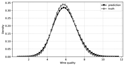
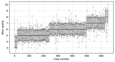
To examine the prediction performance of the estimated conditional density, we construct the 90% prediction interval for the wine quality in the test set. The prediction intervals are shown in the right of fig. 1. The actual wine qualities are plotted in a solid dot. The actual coverage for all 650 cases in the test set is 91.23%, close to the nominal level of 90%.

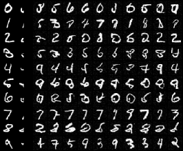
7.3 MNIST handwritten digits

We illustrate the application of Conditional Föllmer Flow to high-dimensional data problems and demonstrate that it can easily handle the models when either of both of $X$ and $Y$ are high-dimensional. The data example we use is the MNIST handwritten digits dataset, which contains 60,000 images for training and 10,000 images for testing. Each image is represented as 28 × 28 matrix with gray color intensity from 0 to 1. Each image is paired with a label in $\{0,1,\cdots,9\}$. We perform Conditional Föllmer Flow on two tasks: generating images from labels and reconstructing missing parts of images given partial observations.

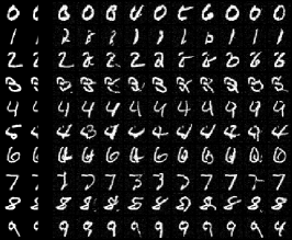
7.3.1 Generating images from labels

We generate images of handwritten digits given the label. In this problem, the predictor $X$ is a categorical variable representing the ten digits: $\{0,1,\cdots,9\}$ and the response $Y$ is the image representation. We use one-hot vectors in $\mathbb{R}^{10}$ to represent $X$. The response $Y\in[0,1]^{784}$ is a vector representing the intensity values.

Refer to caption
Refer to caption
Figure 2: MNIST: real images (left panel) and generated images given labels (right panel).

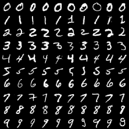
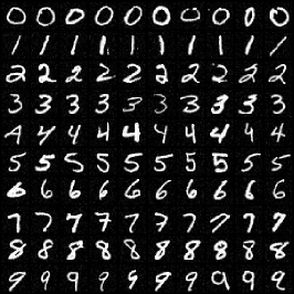
Figure 2 shows the real images (left panel) and generated images (right panel). We see that the generated images are similar to the real images and hard to tell apart from the real images. Also, there are differences in the generated images, reflecting the random variations in the generating process, ensuring the richness of the generating capability.

7.3.2 Reconstructing missing part of an image

We now illustrate using Conditional Föllmer Flow to reconstruct an image when part of the image is missing. Suppose we only observe 1/4, 1/2 or 3/4 of an image and would like to reconstruct the missing part of the image. For this problem, let $X$ be the observed part of the image and let $Y$ be the missing part of the image. Our goal is to reconstruct $Y$ based on $X$.

Refer to caption
Refer to caption
Refer to caption
Figure 3: Reconstructed images given partial image in MNIST dataset. The first column in each panel consists of the true images, the second column consists of the masked images to be reconstructed, the other columns give the constructed images. Left lower 1/4, left 1/2 and 3/4 of the image is observed from left to right, respectively.

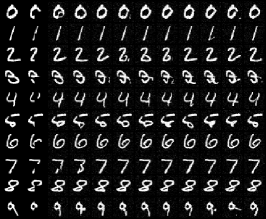
In Figure 3, three plots from left to right corresponds to the situations when 1/4, 1/2 and 3/4 of an image are given. In each plot, the first column contains the true images in the testing set, and the second column consists of the masked images to be reconstructed Each row contains ten reconstructions of the image. If only 1/4 of the digit images are given, it is almost impossible to reconstruct them, except for ”7”. However, as the given area increases, Conditional Föllmer Flow is able to reconstruct the images correctly. For example, for complicate cases such as the digit “2”, if only the left lower 1/4 of the image is given, the reconstructed images tend to be incorrect; the reconstruction is successful when 3/4 of the image is given.

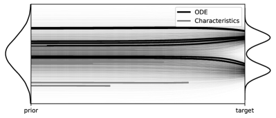
7.4 One step conditional generator

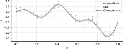
We also explore to capture the characteristic of the ODE flow. Consider the integral operator $\Phi_{t}(x_{0})$, which transforms prior distribution at time 1 to marginal distribution at time $t$. We employ the least square fitting loss to obtain a characteristic neural network, which utilizes a prior $v_{\theta}$ for the numerical integration. Obtaining the characteristic network is in essence a distillation process from the prior velocity estimation. The illustration of ODE based and characteristic based is shown in left of Figure 4. Characteristic based method recovers the trajectory of the ODE system, and maps the initial prior distribution to marginal distributions at any time.

We consider a toy regression problem $Y=1-6X+36X^{2}-53X^{3}+22X^{5}+0.5\sin(6\pi X)+\varepsilon$ where $X\in[0,1]$. We report the results of ODE based and characteristic based method in right of fig. 4. Results show that both methods achieve similar performance.

Refer to caption
Refer to caption
Figure 4: (left) Overview of ODE based and characteristic based generative models. (right) Estimations of different conditional generative models.

8 Conclusion

In this paper, we introduce Conditional Föllmer Flow, an ODE based generative method for sampling from a conditional distribution. We establish that the ODE is defined over the unit time interval, and under mild conditions, the velocity field and flow map of this ODE exhibit Lipschitz properties. Furthermore, we prove that the distribution of the generated samples converges to the underlying target conditional distribution with a certain convergence rate, providing a robust theoretical foundation for our approach. Our numerical experiments showcase its effectiveness across a range of scenarios, from standard nonparametric conditional density estimation problems to more intricate challenges involving image data.

Several questions deserve further investigation. First, we assume the Lipschitz property of $\boldsymbol{v}_{F}$ with respect to the conditional variable $\boldsymbol{y}$, which is crucial for the effective construction of a neural network $\widehat{\boldsymbol{v}}$ to approximate $\boldsymbol{v}_{F}$. Thus, exploring the possibility of obtaining such property under some milder conditions becomes a topic worthy of in-depth scrutiny. Additionally, we demonstrate the regularity of flow map $F_{1}(\cdot,\boldsymbol{y})$, and have explored the use of an additional neural network to preserve information about $\widetilde{F}_{T}(\cdot,\boldsymbol{y})$ to facilitate one-step generation, which can be regarded as directly fitting $F_{1}(\cdot,\boldsymbol{y})$. In fact, $F_{t}(\cdot,\boldsymbol{y})$ exhibits regularity for any $t$. Hence, we can train a time-dependent neural network to approximate $F_{t}(\cdot,\boldsymbol{y})$, i.e. predicting the trajectories or characteristic curves of Conditional Föllmer Flow. Such research will aid in comprehending the mechanisms of generative models, laying foundation for more efficient and stable sampling methods. We plan to thoroughly investigate the aforementioned one-step generator and characteristic curve estimator in the future, also aiming to analyze the convergence properties of these algorithms.

The appendix is organized as follows: In Appendix A, we provide a detailed proof outline. In Appendix B, we prove the approximation error as stated in Theorem 3. In Appendix C, we prove the generalization error as stated in Theorem 4. In Appendix D.1, we provide proof of Proposition 1. In Appendix D.2, we provide proof of Proposition 5 and 6. In Appendix D.3, we provide proof of the main Theorem 2. In Appendix E, we prove related properties of the Conditional Föllmer Flow as stated in Section 3. In Appendix F, we list several useful auxiliary lemmas.

Appendix A Proof Sketch of end-to-end error analysis

A.1 Error analysis of velocity field estimation

We begin with the following connection between the loss function $\mathcal{L}(\boldsymbol{v})$ and the $L^{2}$ approximation error $\left\|\boldsymbol{v}(\cdot,t)-\boldsymbol{v}_{F}(\cdot,t)\right\|_{L^{2}\left(\pi_{t}\right)}$, where $\pi_{t}$ is the joint distribution of $X_{t}=tX_{1}+(1-t)X_{0}$ and $Y$.

Lemma 4

For any velocity field $\boldsymbol{v}:\mathbb{R}^{d}\times\mathbb{R}^{d_{Y}}\times[0,T]\rightarrow\mathbb{R}^{d}$, we have

$$\mathcal{L}(\boldsymbol{v})-\mathcal{L}\left(\boldsymbol{v}_{F}\right)=\frac{1}{T}\int_{0}^{T}\left\|\boldsymbol{v}(\cdot,t)-\boldsymbol{v}_{F}(\cdot,t)\right\|_{L^{2}\left(\pi_{t}\right)}^{2}\mathrm{~{}d}t.$$

Hence, when examining the level of approximation between $\widehat{\boldsymbol{v}}$ and $\boldsymbol{v}_{F}$, we can employ $\mathcal{L}(\widehat{\boldsymbol{v}})-\mathcal{L}\left(\boldsymbol{v}_{F}\right)$ as the error function, which can be further decomposed as:

$$\mathcal{L}(\widehat{\boldsymbol{v}})-\mathcal{L}\left(\boldsymbol{v}_{F}\right)=\underbrace{\mathcal{L}(\widehat{\boldsymbol{v}})-\inf_{\boldsymbol{v}\in\mathrm{NN}}\mathcal{L}(\boldsymbol{v})}_{\text{Generalization error }}+\underbrace{\inf_{\boldsymbol{v}\in\mathrm{NN}}\left(\mathcal{L}(\boldsymbol{v})-\mathcal{L}\left(\boldsymbol{v}_{F}\right)\right)}_{\text{Approximation error }}$$ (11)

A.1.1 Approximation Error

To ensure effective learning, the network class should be expressive enough to approximate the true velocity field. This imposes requirements on the parameters $L,M,J,K$, and $\kappa$, which will be discussed in detail in Theorem 3. A notable aspect of our construction is the ability to impose Lipschitz constant constraints $\left(\gamma_{1},\gamma_{2},\gamma_{3}\right)$ on the neural network functions within the class NN, i.e.

$\displaystyle\left\|\boldsymbol{v}\left(\boldsymbol{x}_{1},\boldsymbol{y},t\right)-\boldsymbol{v}\left(\boldsymbol{x}_{2},\boldsymbol{y},t\right)\right\|_{\infty}\leq\gamma_{1}\left\|\boldsymbol{x}_{1}-\boldsymbol{x}_{2}\right\|,\text{ for any }t\in[0,T],\boldsymbol{y}\in[0,B_{Y}]^{d_{Y}}$
$\displaystyle\left\|\boldsymbol{v}\left(\boldsymbol{x},\boldsymbol{y}_{1},t\right)-\boldsymbol{v}\left(\boldsymbol{x},\boldsymbol{y}_{2},t\right)\right\|_{\infty}\leq\gamma_{2}\left\|\boldsymbol{y}_{1}-\boldsymbol{y}_{2}\right\|,\text{ for any }t\in[0,T],\boldsymbol{x}\in\mathbb{R}^{d}$
$\displaystyle\left\|\boldsymbol{v}\left(\boldsymbol{x},\boldsymbol{y},t_{1}\right)-\boldsymbol{v}\left(\boldsymbol{x},\boldsymbol{y},t_{2}\right)\right\|_{\infty}\leq\gamma_{3}\left|t_{1}-t_{2}\right|,\text{ for any }\boldsymbol{x}\in\mathbb{R}^{d},\boldsymbol{y}\in[0,B_{Y}]^{d_{Y}}$

Extending $\mathrm{FNN}\left(L,M,J,K,\kappa\right)$ to $\mathrm{FNN}\left(L,M,J,K,\kappa,\gamma_{1},\gamma_{2},\gamma_{3}\right)$ will not undermine the approximation power of the neural networks (See the proof of Theorem 3), while it is crucial in bounding the distribution recovery error as demonstrated later in Section A.2. Such construction is enlightened by techniques in work [58], and for brevity, we adopt the proof of work [58]. Our paper differs from [58] in that they assume the score function is Lipschitz uniformly for $t\in[t_{0},T]$, while we derive the Lipschitz property of $\boldsymbol{v}_{F}$ from the assumption on the target distribution.

Theorem 3

Suppose Assumption 1 to 4 hold. Given an approximation error $\epsilon>0$, we choose the hypothesis network class $\mathrm{NN}$ with

$\displaystyle L=\mathcal{O}\left(d+{d_{Y}}+\log\frac{1}{\varepsilon}\right),M=\mathcal{O}\left(\frac{d^{3/2}(\log(d/\varepsilon))^{\frac{d+1}{2}}}{(1-T)^{3}}(B_{Y}\omega)^{d_{Y}}\zeta^{d}\varepsilon^{-(d+{d_{Y}}+1)}\right),$
$\displaystyle J=\mathcal{O}\left(\frac{d^{3/2}(\log(d/\varepsilon))^{\frac{d+1}{2}}}{(1-T)^{3}}(B_{Y}\omega)^{d_{Y}}\zeta^{d}\varepsilon^{-(d+{d_{Y}}+1)}\left(\log\frac{1}{\varepsilon}+d+{d_{Y}}\right)\right),$
$\displaystyle K=\mathcal{O}\left(\frac{\sqrt{d\log\frac{d}{\varepsilon}}}{1-T}\right),\kappa=\mathcal{O}\left(B_{Y}\omega\vee\zeta\sqrt{\log(d/\varepsilon)}\vee\frac{\sqrt{d^{3}\log(d/\varepsilon)}}{(1-T)^{3}}\right)$
$\displaystyle\gamma_{1}=10d^{3/2}\zeta,\,\gamma_{2}=10d_{l}\omega,\,\gamma_{3}=\mathcal{O}\left(\frac{\sqrt{d^{3}\log(d/\varepsilon)}}{(1-T)^{3}}\right)$

There exists an $\widehat{\boldsymbol{v}}_{\boldsymbol{\theta}}\in\mathrm{NN}$, such that for any $t\in[0,T]$, we have

$$\left\|\widehat{\boldsymbol{v}}_{\boldsymbol{\theta}}(\cdot,t)-\boldsymbol{v}_{F}(\cdot,t)\right\|_{L^{2}\left(\pi_{t}\right)}\leq(\sqrt{d+1})\varepsilon$$

where $\pi_{t}$ is the joint distribution of $X_{t}=tX_{1}+(1-t)X_{0}$ and $Y$.

The proof of Theorem 3 can be found in appendix B.

A.1.2 Generalization Error

We define

$$\ell(\bar{\boldsymbol{x}},\boldsymbol{v}):=\frac{1}{T}\int_{0}^{T}\mathbb{E}_{X_{0}}\left[\left\|\left(\boldsymbol{x}-\frac{t}{\sqrt{1-t^{2}}}X_{0}\right)-\boldsymbol{v}\left(t\boldsymbol{x}+\sqrt{1-t^{2}}X_{0},\boldsymbol{y},t\right)\right\|^{2}\right]\mathrm{d}t$$ (12)

where we denote pair $(\boldsymbol{x},\boldsymbol{y})$ as $\bar{\boldsymbol{x}}$. Given $n$ i.i.d. pairs $\left\{X_{1,i},Y_{i}\right\}_{i=1}^{n}$ from $\pi_{1}(\boldsymbol{x},\boldsymbol{y})$, we have the following empirical loss as an interim measure:

$$\bar{\mathcal{L}}(\boldsymbol{v}):=\frac{1}{n}\sum_{i=1}^{n}\ell\left(\bar{X}_{1,i},\boldsymbol{v}\right)$$ (13)

Now the generalization error can be further decomposed into:

$\displaystyle\mathcal{L}(\widehat{\boldsymbol{v}})-\inf_{\boldsymbol{v}\in\mathrm{NN}}\mathcal{L}(\boldsymbol{v})$ $\displaystyle=\mathcal{L}(\widehat{\boldsymbol{v}})-\widehat{\mathcal{L}}(\widehat{\boldsymbol{v}})+\widehat{\mathcal{L}}(\widehat{\boldsymbol{v}})-\widehat{\mathcal{L}}(\widetilde{\boldsymbol{v}})+\widehat{\mathcal{L}}(\widetilde{\boldsymbol{v}})-\mathcal{L}(\widetilde{\boldsymbol{v}})$ (14)
$\displaystyle\leq\mathcal{L}(\widehat{\boldsymbol{v}})-\widehat{\mathcal{L}}(\widehat{\boldsymbol{v}})+\widehat{\mathcal{L}}(\widetilde{\boldsymbol{v}})-\mathcal{L}(\widetilde{\boldsymbol{v}})$
$\displaystyle\leq 2\sup_{\boldsymbol{v}\in\mathrm{NN}}\left|\mathcal{L}(\boldsymbol{v})-\widehat{\mathcal{L}}(\boldsymbol{v})\right|$

where $\widetilde{v}$ is defined in (10). Introducing $\bar{\mathcal{L}}$, we have

$\displaystyle\mathcal{L}(\widehat{\boldsymbol{v}})-\mathcal{L}(\widetilde{\boldsymbol{v}})$ (15)
$\displaystyle\leq$ $\displaystyle 2\sup_{\boldsymbol{v}\in\mathrm{NN}}\left|\mathcal{L}(\boldsymbol{v})-\bar{\mathcal{L}}(\boldsymbol{v})+\bar{\mathcal{L}}(\boldsymbol{v})-\widehat{\mathcal{L}}(\boldsymbol{v})\right|$
$\displaystyle\leq$ $\displaystyle\frac{2}{n}\sup_{\boldsymbol{v}\in\mathrm{NN}}\left|\sum_{i=1}^{n}\left(\mathbb{E}_{\bar{X}_{1}}\left[\ell(\bar{X}_{1},\boldsymbol{v})\right]-\ell\left(\bar{X}_{1,i},\boldsymbol{v}\right)\right)\right|+\frac{2}{n}\sup_{\boldsymbol{v}\in\mathrm{NN}}\left|\sum_{i=1}^{n}\left(\ell\left(\bar{X}_{1,i},\boldsymbol{v}\right)-\widehat{\ell}\left(\bar{X}_{1,i},\boldsymbol{v}\right)\right)\right|$

Let $\mathcal{H}=\left\{\ell(\cdot,\boldsymbol{v}):\boldsymbol{v}\in\mathrm{FNN}\left(L,M,J,K,\kappa,\gamma_{1},\gamma_{2},\gamma_{3}\right)\right\}$, we can employ conventional statistical learning arguments to analyze the first term within $\mathcal{H}$. This is because $\bar{X}_{1}$ and $\bar{X}_{1,i}$ are drawn from $\pi_{1}(\boldsymbol{x},\boldsymbol{y})$, which has bounded support, rendering $\ell(\bar{X}_{1},\boldsymbol{v})$ a bounded random variable. However, the randomness of the second term arises from sampling from $\pi_{0}$ and $U(0,T)$, and since $\pi_{0}$ is unbounded, controlling the second term necessitates an additional truncation argument. Here are some details.

We define $r\left(\left(\boldsymbol{x}_{0},t\right),\bar{\boldsymbol{x}},\boldsymbol{v}\right)=\left\|\boldsymbol{x}-\frac{t}{\sqrt{1-t^{2}}}\boldsymbol{x}_{0}-\boldsymbol{v}\left(t\boldsymbol{x}+\sqrt{1-t^{2}}\boldsymbol{x}_{0},\boldsymbol{y},t\right)\right\|^{2}$ and the truncation version $r^{\text{trunc }}\left(\left(\boldsymbol{x}_{0},t\right),\bar{\boldsymbol{x}},\boldsymbol{v}\right)=r\left(\left(\boldsymbol{x}_{0},t\right),\bar{\boldsymbol{x}},\boldsymbol{v}\right)\mathbb{I}\left\{\left\|\boldsymbol{x}_{0}\right\|_{\infty}\leq D\right\}$, where $D$ will be determined later. Thus, we express $\ell\left(\bar{X}_{1,i},\boldsymbol{v}\right)=\mathbb{E}_{t,X_{0}}\left[r\left(\left(X_{0},t\right),\bar{X}_{1,i},\boldsymbol{v}\right)\right]$, while defining $\ell^{\text{trunc }}(\bar{X}_{1,i},\boldsymbol{v})$ similarly. We also have $\widehat{\ell}^{\text{trunc }}(\bar{X}_{1,i},\boldsymbol{v})=\frac{1}{m}\sum_{j=1}^{m}r^{\text{trunc }}\left(\left(X_{0,j},t_{j}\right),\bar{X}_{1,i},\boldsymbol{v}\right)$ given $m$ i.i.d. sample $\left\{\left(X_{0,j},t_{j}\right)\right\}_{j=1}^{m}$ from $\pi_{0}$ and $U(0,T)$.

Now, the second term has the following decomposition:

$\displaystyle\frac{1}{n}\sup_{\boldsymbol{v}\in\mathrm{NN}}\left|\sum_{i=1}^{n}\left(\ell\left(\bar{X}_{1,i},\boldsymbol{v}\right)-\widehat{\ell}\left(\bar{X}_{1,i},\boldsymbol{v}\right)\right)\right|$ (16)
$\displaystyle\leq$ $\displaystyle\underbrace{\frac{1}{n}\sum_{i=1}^{n}\sup_{\boldsymbol{v}\in\mathrm{NN}}\left|\ell\left(\bar{X}_{1,i},\boldsymbol{v}\right)-\ell^{\text{trunc}}\left(\bar{X}_{1,i},\boldsymbol{v}\right)\right|}_{\text{Truncation Error (I) }}+\underbrace{\frac{1}{n}\sum_{i=1}^{n}\sup_{\boldsymbol{v}\in\mathrm{NN}}\left|\widehat{\ell}\left(\bar{X}_{1,i},\boldsymbol{v}\right)-\widehat{\ell}^{\text{trunc}}\left(\bar{X}_{1,i},\boldsymbol{v}\right)\right|}_{\text{Truncation Error (II) }}$
$\displaystyle+\underbrace{\frac{1}{n}\sum_{i=1}^{n}\sup_{\boldsymbol{v}\in\mathrm{NN}}\left|\ell^{\text{trunc}}\left(\bar{X}_{1,i},\boldsymbol{v}\right)-\widehat{\ell}^{\text{trunc}}\left(\bar{X}_{1,i},\boldsymbol{v}\right)\right|}_{\text{Statistical Error }}$

We now can use conventional statistical learning arguments to analyze Statistical Error term. Regarding the two Truncation Error terms, we leverage the tail properties of Gaussian variables.

Based on above discussion and Theorem 3, we derive the following generalization bound:

Theorem 4

Suppose Assumption 1 to 4 hold. Given $n$ samples $\left\{(X_{1,i},Y_{i})\right\}_{i=1}^{n}$ from $\pi_{1}(\boldsymbol{x},\boldsymbol{y})$ and $m$ samples $\left\{\left(X_{0,j},t_{j}\right)\right\}_{j=1}^{m}$ jointly from $\pi_{0}$ and $U(0,T)$, we choose network class as in Theorem 3 with $\varepsilon=n^{-\frac{1}{d+{d_{Y}}+5}}$. By setting $m=n$, with probability of at least $1-\frac{1}{n^{2}}$, we obtain the convergence rate of order

$$\frac{1}{T}\int_{0}^{T}\left\|\widehat{\boldsymbol{v}}(\cdot,t)-\boldsymbol{v}_{F}(\cdot,t)\right\|_{L^{2}\left(\pi_{t}\right)}^{2}\mathrm{~{}d}t=\widetilde{\mathcal{O}}\left(\frac{\zeta^{d/2}\omega^{{d_{Y}}/2}}{(1-T)^{7/2}}n^{-\frac{2}{d+d_{Y}+5}}\right),$$

where we omit factors in $d,\log n,\log m,\log(1-T)$.

The complete proof of Theorem 4, together with the upper bound analysis of $\ell(\cdot,\boldsymbol{v})$ and covering number evaluation of $\mathcal{H}$, are presented in Appendix C.

A.2 Error analysis of sampling process

We first consider the target Conditional Föllmer Flow:

$$\mathrm{d}Z^{\boldsymbol{y}}_{t}=\boldsymbol{v}_{F}\left(Z_{t}^{\boldsymbol{y}},\boldsymbol{y},t\right)\mathrm{d}t,\,\,Z^{\boldsymbol{y}}_{0}\sim\pi_{0},\,\,0\leq t\leq T$$

And what we can expect is the estimated velocity field $\widehat{\boldsymbol{v}}$:

$$\mathrm{d}\widehat{Z}^{\boldsymbol{y}}_{t}=\widehat{\boldsymbol{v}}\left(\widehat{Z}^{\boldsymbol{y}}_{t},\boldsymbol{y},t\right)\mathrm{d}t,\,\,\widehat{Z}^{\boldsymbol{y}}_{0}\sim\pi_{0},\,\,0\leq t\leq T$$

Denote the distribution of $F_{t}\left(Z_{0},\boldsymbol{y}\right)$ and $\widehat{F}_{t}\left(Z_{0},\boldsymbol{y}\right)$ by $\pi^{\boldsymbol{y}}_{t}$ and $\widehat{\pi}^{\boldsymbol{y}}_{t}$ respectively, where $Z_{0}\sim\pi_{0}$ and $\widehat{F}_{t}\left(\cdot,\boldsymbol{y}\right)$ denotes the flow map related to $\widehat{Z}^{\boldsymbol{y}}_{t}$. We have the following estimate of the Wasserstein-2 distance $W_{2}\left(\pi^{\boldsymbol{y}}_{T},\widehat{\pi}^{\boldsymbol{y}}_{T}\right)$

Proposition 1

Suppose Assumption 1 to 4 hold. Given $n$ samples $\left\{(X_{1,i},Y_{i})\right\}_{i=1}^{n}$ from $\pi_{1}(\boldsymbol{x},\boldsymbol{y})$ and $m$ samples $\left\{\left(X_{0,j},t_{j}\right)\right\}_{j=1}^{m}$ jointly from $\pi_{0}$ and $U(0,T)$, we choose network class as in Theorem 3 with $\varepsilon=n^{-\frac{1}{d+d_{Y}+5}}$. Then, with probability of at least $1-\frac{1}{n^{2}}$, it holds

$$\mathbb{E}_{\boldsymbol{y}\sim\pi(\boldsymbol{y})}\left[W^{2}_{2}\left(\pi^{\boldsymbol{y}}_{T},\widehat{\pi}^{\boldsymbol{y}}_{T}\right)\right]=\widetilde{\mathcal{O}}\left(e^{2d^{1/2}\gamma_{1}}\frac{\zeta^{d/2}\omega^{{d_{Y}}/2}}{(1-T)^{7/2}}n^{-\frac{2}{d+d_{Y}+5}}\right)$$

where $\pi(\boldsymbol{y})$ denotes the distribution of the predictor $Y$.

The proof of Proposition 1 is deferred to Appendix D.1. Now consider the Euler method:

$$\mathrm{d}\widetilde{Z}^{\boldsymbol{y}}_{t}=\widehat{\boldsymbol{v}}\left(\widetilde{Z}^{\boldsymbol{y}}_{t_{k}},\boldsymbol{y},t_{k}\right)\mathrm{d}t,\quad\widetilde{Z}_{0}^{\boldsymbol{y}}\sim\pi_{0},\quad t_{k}\leq t\leq t_{k+1},\quad k=0,1,\ldots,N-1$$

we denote the distribution of $\widetilde{F}_{t}\left(Z_{0},\boldsymbol{y}\right)$ by $\widetilde{\pi}^{\boldsymbol{y}}_{T}$, where $Z_{0}\sim\pi_{0}$ and $\widetilde{F}_{t}\left(\cdot,\boldsymbol{y}\right)$ denotes the flow map related to $\widetilde{Z}^{\boldsymbol{y}}_{t}$. To establish the distribution recovery guarantees, we need the following discretization error bound:

Lemma 5

Let $0=t_{0}<t_{1}<\cdots<t_{N}=T$ be the discretization points. For any neural network $\widehat{\boldsymbol{v}}$ in $\mathrm{FNN}\left(L,M,J,K,\kappa,\gamma_{1},\gamma_{2},\gamma_{3}\right)$, and for any $\boldsymbol{y}\in[0,B_{Y}]^{d_{Y}}$, we can assert the following

$$W_{2}\left(\widehat{\pi}^{\boldsymbol{y}}_{T},\widetilde{\pi}^{\boldsymbol{y}}_{T}\right)=\mathcal{O}\left(e^{\gamma_{1}}\left(\gamma_{1}K+\gamma_{3}\right)\sqrt{\sum_{k=0}^{N-1}\left(t_{k+1}-t_{k}\right)^{3}}\right)$$

whose proof can be found in Appendix D.2.

We finally attain a trade-off on stopping time $T$ in the following lemma:

Lemma 6

Suppose Assumption 2 holds, for any $\boldsymbol{y}\in[0,B_{Y}]^{d_{Y}}$, we have

$$W_{2}\left(\pi^{\boldsymbol{y}}_{T},\pi^{\boldsymbol{y}}_{1}\right)\lesssim\sqrt{d(1-T)}$$

The proof of which is also deferred to Appendix D.2. Proposition 1 demonstrates that as stopping time $T$ tends to $1$, the error of using the estimated velocity field in the sampling dynamics increases. Conversely, according to Lemma 6, the distance between $\pi^{\boldsymbol{y}}_{T}$ and $\pi^{\boldsymbol{y}}_{1}$ decreases as $T$ approaches $1$. This reveals a trade-off in the stopping time $T$ between the error in velocity field estimation and the distribution recovery.

Appendix B Approximation Error

B.1 Proof of Theorem 3

The goal is to find a network $\widehat{\boldsymbol{v}}$ in NN to approximate the true vector field $\boldsymbol{v}_{F}$. A major difficulty in approximating $\boldsymbol{v}_{F}(\boldsymbol{x},\boldsymbol{y},t)$ is that the input space $\mathbb{R}^{d}\times[0,B_{Y}]^{d_{Y}}\times[0,T]$ is unbounded. To address this difficulty, we partition $\mathbb{R}^{d}$ into a compact subset $\mathcal{K}$ and its complement $\mathcal{K}^{c}$.

Firstly, we consider the approximation on $\mathcal{K}\times[0,B_{Y}]^{d_{Y}}\times[0,T]$. Let $\mathcal{K}=\left\{\boldsymbol{x}\mid\|\boldsymbol{x}\|_{\infty}\leq R\right\}$ to be a $d$-dimensional hypercube with edge length $2R>0$, where $R$ will be determined later. On $\mathcal{K}\times[0,B_{Y}]^{d_{Y}}\times[0,T]$, we approximate $k$-coordinate maps $v_{F}^{k}(\boldsymbol{x},\boldsymbol{y},t)$ separately, where $\boldsymbol{v}_{F}=\left[v_{F}^{1}(\boldsymbol{x},\boldsymbol{y},t),\cdots,v_{F}^{d}(\boldsymbol{x},\boldsymbol{y},t)\right]^{T}$.

we will rescale the input by $\boldsymbol{x}^{\prime}=\frac{1}{2R}(\boldsymbol{x}+R\mathbf{1})$, $\boldsymbol{y}^{\prime}=\boldsymbol{y}/B_{Y}$ and $t^{\prime}=t/T$, where $\mathbf{1}:=[1,\cdots,1]^{T}$, so that the transformed space is $[0,1]^{d+{d_{Y}}+1}$. Such a transformation can be exactly implemented by a single ReLU layer.

By Lemma 1, $\boldsymbol{v}_{F}(\boldsymbol{x},\boldsymbol{y},t)$ is $\zeta$-Lipschitz in $\boldsymbol{x}$. We define the rescaled function on the transformed input space as $\boldsymbol{v}\left(\boldsymbol{x}^{\prime},\boldsymbol{y}^{\prime},t^{\prime}\right):=\boldsymbol{v}_{F}\left(2R\boldsymbol{x}^{\prime}-R\mathbf{1},B_{Y}\boldsymbol{y}^{\prime},Tt^{\prime}\right)$, so that $\boldsymbol{v}$ is $2\zeta R$-Lipschitz in $\boldsymbol{x}^{\prime}$. Further by Assumption 4, $\boldsymbol{v}$ is $B_{Y}\omega$-Lipschitz in $\boldsymbol{y}^{\prime}$.

We also denote the Lipschitz constant of $\boldsymbol{v}\left(\boldsymbol{x}^{\prime},\boldsymbol{y}^{\prime},t^{\prime}\right)$ w.r.t. $t^{\prime}$ as $T\tau(R)$, when $\boldsymbol{x}^{\prime}\in[0,1]^{d}$. We denote $\tau(R):=\sup_{t\in[0,T]}\sup_{\boldsymbol{y}\in[0,B_{Y}]^{d_{Y}}}\sup_{\boldsymbol{x}\in[-R,R]^{d}}\left\|\partial_{t}\boldsymbol{v}_{F}\right\|$.

An upper bound for $\tau(R)$ is computed in Lemma 15 by $\tau(R)=\mathcal{O}\left(\frac{d^{3/2}(R+1)}{(1-T)^{3}}\right)$. Now the goal becomes approximating $\boldsymbol{v}$ on $[0,1]^{d+{d_{Y}}+1}$.

Second, we partition $[0,1]^{d}$ into non-overlapping hypercubes with equal edge length $e_{1}$, and $[0,1]^{d_{Y}}$ into equal edge length $e_{2}$. We also partition the time interval $[0,1]$ into non-overlapping sub-intervals of length $e_{3}$. $e_{1}$, $e_{2}$ and $e3$ will be chosen depending on the desired approximation error. We denote $N_{1}=\left\lceil\frac{1}{e_{1}}\right\rceil$, $N_{2}=\left\lceil\frac{1}{e_{2}}\right\rceil$ and $N_{3}=\left\lceil\frac{1}{e_{3}}\right\rceil$.

Let $\boldsymbol{p}=\left[p_{1},\cdots,p_{d}\right]^{T}\in\left[N_{1}\right]^{d}$, $\boldsymbol{q}=\left[q_{1},\cdots,q_{m}\right]^{T}\in\left[N_{2}\right]^{d_{Y}}$ be multi-indexes. We define $\overline{\boldsymbol{v}}$ as

$$\bar{v}_{i}\left(\boldsymbol{x}^{\prime},\boldsymbol{y}^{\prime},t^{\prime}\right):=\sum_{\boldsymbol{p}\in\left[N_{1}\right]^{d},\boldsymbol{q}\in\left[N_{2}\right]^{d_{Y}},j\in\left[N_{2}\right]}v_{F}^{i}\left(2R\frac{\boldsymbol{p}}{N_{1}}-R\mathbf{1},B_{Y}\frac{\boldsymbol{q}}{N_{2}},T\frac{j}{N_{3}}\right)\Psi_{\boldsymbol{p},\boldsymbol{q},j}\left(\boldsymbol{x}^{\prime},\boldsymbol{y}^{\prime},t^{\prime}\right)$$

where $\Psi_{\boldsymbol{p},\boldsymbol{q},j}\left(\boldsymbol{x}^{\prime},\boldsymbol{y}^{\prime},t^{\prime}\right)$ is a partition of unity function, that is

$$\sum_{\boldsymbol{p}\in\left[N_{1}\right]^{d},\boldsymbol{q}\in\left[N_{2}\right]^{d},j\in\left[N_{3}\right]}\Psi_{\boldsymbol{p},\boldsymbol{q},j}\left(\boldsymbol{x}^{\prime},\boldsymbol{y}^{\prime},t^{\prime}\right)\equiv 1,\,on\quad[0,1]^{d}\times[0,1]^{d_{Y}}\times[0,1]$$

We choose $\Psi_{\boldsymbol{p},\boldsymbol{q},j}$ as a product of coordinate-wise trapezoid functions:

$$\Psi_{\boldsymbol{p},\boldsymbol{q},j}:=\psi\left(3N_{3}\left(t^{\prime}-\frac{j}{N_{3}}\right)\right)\prod_{i=1}^{m}\psi\left(3N_{2}\left(x_{i}^{\prime}-\frac{q_{i}}{N_{2}}\right)\right)\prod_{i=1}^{d}\psi\left(3N_{1}\left(x_{i}^{\prime}-\frac{p_{i}}{N_{1}}\right)\right)$$

where $\psi$ is a trapezoid function,

$$\psi(a):=\begin{cases}1,&|a|<1\\ 2-|a|,&|a|\in[1,2]\\ 0,&|a|>2\end{cases}$$

We claim that $\bar{v}_{i}$ is an approximation of $v_{i}$, and $\bar{v}_{i}$ can be implemented by a ReLU neural network $\widehat{v}_{i}$ with small error.

Both claims are verified in Lemma 10 of [70], where we only need to substitute the Lipschitz constant $2\zeta R$ , $B_{Y}\omega$ and $T\tau(R)$ into the error analysis. We use the coordinate-wise analysis in the proof of Lemma 10 of [70] for deriving the Lipschitz continuity w.r.t. $\boldsymbol{x}^{\prime}$, $\boldsymbol{y}^{\prime}$ and $t^{\prime}$. Similar proofs can be found in [71]. By concatenating $\widehat{v}_{i}$ ’s together, we construct $\widehat{\boldsymbol{v}}_{\boldsymbol{\theta}}=\left[\widehat{v}_{1},\ldots,\widehat{v}_{d}\right]^{T}$. Given $\varepsilon$, if we achieve

$$\sup_{(\boldsymbol{x}^{\prime},\boldsymbol{y}^{\prime},t^{\prime})\in[0,1]^{d}\times[0,1]^{d_{Y}}\times[0,1]}\left\|\widehat{\boldsymbol{v}}_{\boldsymbol{\theta}}\left(\boldsymbol{x}^{\prime},\boldsymbol{y}^{\prime},t^{\prime}\right)-\boldsymbol{v}\left(\boldsymbol{x}^{\prime},\boldsymbol{y}^{\prime},t^{\prime}\right)\right\|_{\infty}\leq\varepsilon$$

the neural network configuration is

$$\begin{gathered}L=\mathcal{O}\left(\log\frac{1}{\varepsilon}+d+{d_{Y}}\right),M=\mathcal{O}\left(T\tau(R)(\zeta R)^{d}(B_{Y}\omega)^{d_{Y}}\varepsilon^{-(d+{d_{Y}}+1)}\right),\\ J=\mathcal{O}\left(T\tau(R)(\zeta R)^{d}(B_{Y}\omega)^{d_{Y}}\varepsilon^{-(d+{d_{Y}}+1)}\left(\log\frac{1}{\varepsilon}+d+{d_{Y}}\right)\right),\\ K=\mathcal{O}\left(\frac{\sqrt{d}R}{1-T}\right),\kappa=\max\{1,\zeta R,T\tau(R),B_{Y}\omega\}\end{gathered}$$

Here we already take $e_{1}=\mathcal{O}\left(\frac{\varepsilon}{\zeta R}\right)$, $e_{2}=\mathcal{O}\left(\frac{\varepsilon}{T\tau(R)}\right)$ and $e_{3}=\mathcal{O}\left(\frac{\varepsilon}{B_{Y}\omega}\right)$. The output range $K$ is computed by $K=\sqrt{d}\max_{i}\sup_{(\boldsymbol{x},\boldsymbol{y},t)\in[-R,R]^{d}\times[0,B_{Y}]^{d_{Y}}\times[0,T]}\left\|v_{F}^{i}(\boldsymbol{x},\boldsymbol{y},t)\right\|$. Combining with the input transformation layer, i.e., $\boldsymbol{x}\rightarrow\boldsymbol{x}^{\prime}$, $\boldsymbol{y}\rightarrow\boldsymbol{y}^{\prime}$ and $t\rightarrow t^{\prime}$ rescaling, the constructed network is locally Lipschitz continuous in $\boldsymbol{x}$, i.e., for any $\boldsymbol{x}_{1},\boldsymbol{x}_{2}\in\mathcal{K}$ and $t\in[0,T]$, $\boldsymbol{y}\in[0,B_{Y}]^{d_{Y}}$, it holds

$$\left\|\widehat{\boldsymbol{v}}_{\boldsymbol{\theta}}\left(\boldsymbol{x}_{1},\boldsymbol{y},t\right)-\widehat{\boldsymbol{v}}_{\boldsymbol{\theta}}\left(\boldsymbol{x}_{2},\boldsymbol{y},t\right)\right\|_{\infty}\leq 10d\zeta\left\|\boldsymbol{x}_{1}-\boldsymbol{x}_{2}\right\|$$

Moreover, the network is also Lipschitz in $\boldsymbol{y}$ and $t$, i.e., for any $\boldsymbol{y}_{1},\boldsymbol{y}_{2}\in[0,B_{Y}]^{d_{Y}}$ and $\|\boldsymbol{x}\|_{\infty}\leq R$, $t\in[0,T]$, it holds

$$\left\|\widehat{\boldsymbol{v}}_{\boldsymbol{\theta}}\left(\boldsymbol{x},\boldsymbol{y}_{1},t\right)-\widehat{\boldsymbol{v}}_{\boldsymbol{\theta}}\left(\boldsymbol{x},\boldsymbol{y}_{2},t\right)\right\|_{\infty}\leq 10{d_{Y}}\omega\left\|\boldsymbol{y}_{1}-\boldsymbol{y}_{2}\right\|$$

And for any $t_{1},t_{2}\in[1,T]$ and $\|\boldsymbol{x}\|_{\infty}\leq R$, $\boldsymbol{y}\in[0,B_{Y}]^{d_{Y}}$, it holds

$$\left\|\widehat{\boldsymbol{v}}_{\boldsymbol{\theta}}\left(\boldsymbol{x},\boldsymbol{y},t_{1}\right)-\widehat{\boldsymbol{v}}_{\boldsymbol{\theta}}\left(\boldsymbol{x},\boldsymbol{y},t_{2}\right)\right\|_{\infty}\leq 10\tau(R)\left|t_{1}-t_{2}\right|$$

In order to ensure global Lipschitz continuity of $\widehat{\boldsymbol{v}}_{\boldsymbol{\theta}}$ with respect to $\boldsymbol{x}$, we introduce the following lemma.

Lemma 7

For $\mathcal{K}=\left\{\boldsymbol{x}\in\mathbb{R}^{d}\mid\|\boldsymbol{x}\|_{\infty}\leq R\right\}$, there exists an $\mathrm{1}$-Lipschitz map $\mathcal{T}_{\mathcal{K}}:\mathbb{R}^{d}\to\mathcal{K}$, which satisfies $\mathcal{T}_{\mathcal{K}}(\boldsymbol{x})=\boldsymbol{x}$, for any $\boldsymbol{x}\in\mathcal{K}$. Further, $\mathcal{T}_{\mathcal{K}}$ can be expressed as an $\mathrm{2}$-layer ReLU network with width order $\mathcal{O}(d)$.

Proof 1

Consider the following univariate real-valued function

$$T_{R}(\boldsymbol{x}):=\begin{cases}R,&x>R\\ x,&x\in[-R,R]\\ -R,&x<-R\end{cases}$$

Now define $\mathcal{T}_{\mathcal{K}}(\boldsymbol{x})=\mathcal{T}_{\mathcal{K}}(x_{1},x_{2},...,x_{d})=(T_{R}(x_{1}),T_{R}(x_{2}),...,T_{R}(x_{d}))$, immediately it yields that $\mathcal{T}_{\mathcal{K}}(\boldsymbol{x})=\boldsymbol{x},\boldsymbol{x}\in\mathcal{K}$. For $\boldsymbol{x}\in\mathcal{K}^{c}$, $\mathcal{T}_{\mathcal{K}}(\boldsymbol{x})\in\partial\mathcal{K}$.

Simple calculation tells us

$\displaystyle\left\|\mathcal{T}_{\mathcal{K}}(\boldsymbol{x})-\mathcal{T}_{\mathcal{K}}(\boldsymbol{y})\right\|_{\infty}=$ $\displaystyle\max_{i=1,...,d}\left|T_{R}(x_{i})-T_{R}(y_{i})\right|$
$\displaystyle\leq$ $\displaystyle\max_{i=1,...,d}\left|x_{i}-y_{i}\right|=\left\|\boldsymbol{x}-\boldsymbol{y}\right\|_{\infty}\leq\left\|\boldsymbol{x}-\boldsymbol{y}\right\|$

Also, it’s easy to check

$$T_{R}(\boldsymbol{x})=\text{ReLU}(\boldsymbol{x})-\text{ReLU}(-x)+\text{ReLU}(-x-R)-\text{ReLU}(x-R)$$

It concludes the proof.

We now consider $\mathrm{NN}$ function $\widehat{\boldsymbol{v}}_{\boldsymbol{\theta}}(\mathcal{T}_{\mathcal{K}}(\boldsymbol{x}),\boldsymbol{y},t)$. Firstly it preserves the approximation capability of $\widehat{\boldsymbol{v}}_{\boldsymbol{\theta}}$, i.e.

$\displaystyle\sup_{(\boldsymbol{x},\boldsymbol{y},t)\in\mathcal{K}\times[0,B_{Y}]^{d_{Y}}\times[0,T]}\left\|\widehat{\boldsymbol{v}}_{\boldsymbol{\theta}}\left(\mathcal{T}_{\mathcal{K}}(\boldsymbol{x}),\boldsymbol{y},t\right)-\boldsymbol{v}_{F}\left(\boldsymbol{x},\boldsymbol{y},t\right)\right\|_{\infty}$
$\displaystyle=$ $\displaystyle\sup_{(\boldsymbol{x},\boldsymbol{y},t)\in\mathcal{K}\times[0,B_{Y}]^{d_{Y}}\times[0,T]}\left\|\widehat{\boldsymbol{v}}_{\boldsymbol{\theta}}\left(\boldsymbol{x},\boldsymbol{y},t\right)-\boldsymbol{v}_{F}\left(\boldsymbol{x},\boldsymbol{y},t\right)\right\|_{\infty}\leq\varepsilon$

Then, obviously

$\displaystyle\sup_{(\boldsymbol{x},\boldsymbol{y},t)\in\mathbb{R}^{d}\times[0,B_{Y}]^{d_{Y}}\times[0,T]}\left\|\widehat{\boldsymbol{v}}_{\boldsymbol{\theta}}\left(\mathcal{T}_{\mathcal{K}}(\boldsymbol{x}),\boldsymbol{y},t\right)\right\|=$ $\displaystyle\sup_{(\boldsymbol{x},\boldsymbol{y},t)\in\mathcal{K}\times[0,B_{Y}]^{d_{Y}}\times[0,T]}\left\|\widehat{\boldsymbol{v}}_{\boldsymbol{\theta}}\left(\boldsymbol{x},\boldsymbol{y},t\right)\right\|=\,K$

Finally, since $\mathcal{T}_{\mathcal{K}}(\mathbb{R}^{d})=\mathcal{K}$, for any $\boldsymbol{x}_{1},\boldsymbol{x}_{2}\in\mathbb{R}^{d}$ and $t\in[0,T]$, $\boldsymbol{y}\in[0,B_{Y}]^{d_{Y}}$, it holds

$\displaystyle\left\|\widehat{\boldsymbol{v}}_{\boldsymbol{\theta}}\left(\mathcal{T}_{\mathcal{K}}(\boldsymbol{x}_{1}),\boldsymbol{y},t\right)-\widehat{\boldsymbol{v}}_{\boldsymbol{\theta}}\left(\mathcal{T}_{\mathcal{K}}(\boldsymbol{x}_{2}),\boldsymbol{y},t\right)\right\|_{\infty}\leq$ $\displaystyle 10d\zeta\left\|\mathcal{T}_{\mathcal{K}}(\boldsymbol{x}_{1})-\mathcal{T}_{\mathcal{K}}(\boldsymbol{x}_{2})\right\|$
$\displaystyle\leq$ $\displaystyle 10d^{3/2}\zeta\left\|\mathcal{T}_{\mathcal{K}}(\boldsymbol{x}_{1})-\mathcal{T}_{\mathcal{K}}(\boldsymbol{x}_{2})\right\|_{\infty}$
$\displaystyle\leq$ $\displaystyle 10d^{3/2}\zeta\left\|\boldsymbol{x}_{1}-\boldsymbol{x}_{2}\right\|$

So $\widehat{\boldsymbol{v}}_{\boldsymbol{\theta}}\left(\mathcal{T}_{\mathcal{K}}(\boldsymbol{x}),\boldsymbol{y},t\right)$ acquires global Lipschitz continuity with respect to $\boldsymbol{x}$. From now on, we use $\widehat{\boldsymbol{v}}_{\boldsymbol{\theta}}$ to denote $\widehat{\boldsymbol{v}}_{\boldsymbol{\theta}}\left(\mathcal{T}_{\mathcal{K}}(\boldsymbol{x}),\boldsymbol{y},t\right)$.

The $L^{2}$ approximation error of $\widehat{\boldsymbol{v}}_{\boldsymbol{\theta}}$ can be decomposed into two terms,

$\displaystyle\left\|\boldsymbol{v}_{F}(\boldsymbol{x},\boldsymbol{y},t)-\widehat{\boldsymbol{v}}_{\boldsymbol{\theta}}(\boldsymbol{x},\boldsymbol{y},t)\right\|^{2}_{L^{2}\left(\pi_{t}\right)}=$ $\displaystyle\left\|\left(\boldsymbol{v}_{F}(\boldsymbol{x},\boldsymbol{y},t)-\widehat{\boldsymbol{v}}_{\boldsymbol{\theta}}(\boldsymbol{x},\boldsymbol{y},t)\right)\mathbb{I}\left\{\|\boldsymbol{x}\|_{\infty}\leq R\right\}\right\|^{2}_{L^{2}\left(\pi_{t}\right)}$
$\displaystyle+\left\|\left(\boldsymbol{v}_{F}(\boldsymbol{x},\boldsymbol{y},t)-\widehat{\boldsymbol{v}}_{\boldsymbol{\theta}}(\boldsymbol{x},\boldsymbol{y},t)\right)\mathbb{I}\left\{\|\boldsymbol{x}\|_{\infty}>R\right\}\right\|^{2}_{L^{2}\left(\pi_{t}\right)}$

The first term on the right-hand side of the last display is bounded by

$\displaystyle\left\|\left(\boldsymbol{v}_{F}-\widehat{\boldsymbol{v}}_{\boldsymbol{\theta}}\right)\mathbb{I}\left\{\|\boldsymbol{x}\|_{\infty}\leq R\right\}\right\|^{2}_{L^{2}\left(\pi_{t}\right)}$ $\displaystyle\leq d\sup_{(\boldsymbol{x},\boldsymbol{y},t)\in\mathcal{K}\times[0,B_{Y}]^{d_{Y}}\times[0,T]}\left\|\boldsymbol{v}_{F}(\boldsymbol{x},\boldsymbol{y},t)-\widehat{\boldsymbol{v}}_{\boldsymbol{\theta}}(\boldsymbol{x},\boldsymbol{y},t)\right\|^{2}_{\infty}$
$\displaystyle\leq d\varepsilon^{2}$

The second term admits an upper bound in Lemma 8. Specifically, when choosing $R=\mathcal{O}\left(\sqrt{\log\frac{d}{\varepsilon}}\right)$, we have

$$\left\|\left(\boldsymbol{v}_{F}(\boldsymbol{x},\boldsymbol{y},t)-\widehat{\boldsymbol{v}}_{\boldsymbol{\theta}}(\boldsymbol{x},\boldsymbol{y},t)\right)\mathbb{I}\left\{\|\boldsymbol{x}\|_{\infty}>R\right\}\right\|^{2}_{L^{2}\left(\pi_{t}\right)}\leq\varepsilon^{2}$$

As a result, with the choice of $R$, we obtain

$$\left\|\boldsymbol{v}_{F}(\boldsymbol{x},\boldsymbol{y},t)-\widehat{\boldsymbol{v}}_{\boldsymbol{\theta}}(\boldsymbol{x},\boldsymbol{y},t)\right\|_{L^{2}\left(\pi_{t}\right)}\leq\sqrt{d+1}\varepsilon$$

Substituting $R$ into the network configuration, we obtain

$\displaystyle L=\mathcal{O}\left(d+{d_{Y}}+\log\frac{1}{\varepsilon}\right),M=\mathcal{O}\left(\frac{d^{3/2}(\log(d/\varepsilon))^{\frac{d+1}{2}}}{(1-T)^{3}}(B_{Y}\omega)^{d_{Y}}\zeta^{d}\varepsilon^{-(d+{d_{Y}}+1)}\right),$
$\displaystyle J=\mathcal{O}\left(\frac{d^{3/2}(\log(d/\varepsilon))^{\frac{d+1}{2}}}{(1-T)^{3}}(B_{Y}\omega)^{d_{Y}}\zeta^{d}\varepsilon^{-(d+{d_{Y}}+1)}\left(\log\frac{1}{\varepsilon}+d+{d_{Y}}\right)\right),$
$\displaystyle K=\mathcal{O}\left(\frac{\sqrt{d\log\frac{d}{\varepsilon}}}{1-T}\right),\kappa=\mathcal{O}\left(B_{Y}\omega\vee\zeta\sqrt{\log(d/\varepsilon)}\vee\frac{\sqrt{d^{3}\log(d/\varepsilon)}}{(1-T)^{3}}\right)$
$\displaystyle\gamma_{1}=10d^{3/2}\zeta,\,\gamma_{2}=10d_{l}\omega,\,\gamma_{3}=\mathcal{O}\left(\frac{\sqrt{d^{3}\log(d/\varepsilon)}}{(1-T)^{3}}\right)$

B.2 Truncation error

Lemma 8

Under Assumption 1 and 2, given $\varepsilon>0$, with $R=\mathcal{O}\left(\sqrt{\log\frac{d}{\varepsilon}}\right)$

$$\left\|\left(\boldsymbol{v}_{F}(\boldsymbol{x},\boldsymbol{y},t)-\widehat{\boldsymbol{v}}_{\boldsymbol{\theta}}(\boldsymbol{x},\boldsymbol{y},t)\right)\mathbb{I}\left\{\|\boldsymbol{x}\|_{\infty}>R\right\}\right\|^{2}_{L^{2}\left(\pi_{t}\right)}\leq\varepsilon^{2}.$$
Proof 2

For any $R>0$, using the identity $\boldsymbol{v}_{F}=\mathbb{E}[X_{1}-\frac{t}{\sqrt{1-t^{2}}}X_{0}|X_{t}=\boldsymbol{x},Y=\boldsymbol{y}]$, we have

$\displaystyle\left\|\left(\boldsymbol{v}_{F}(\boldsymbol{x},\boldsymbol{y},t)-\widehat{\boldsymbol{v}}_{\boldsymbol{\theta}}(\boldsymbol{x},\boldsymbol{y},t)\right)\mathbb{I}\left\{\|\boldsymbol{x}\|_{\infty}>R\right\}\right\|^{2}_{L^{2}\left(\pi_{t}\right)}$ (17)
$\displaystyle=$ $\displaystyle\int_{\|\boldsymbol{x}\|_{\infty}>R}\left\|\boldsymbol{v}_{F}(\boldsymbol{x},\boldsymbol{y},t)-\widehat{\boldsymbol{v}}_{\boldsymbol{\theta}}(\boldsymbol{x},\boldsymbol{y},t)\right\|^{2}\pi_{t}(\mathrm{d}\boldsymbol{x},\mathrm{d}\boldsymbol{y})$
$\displaystyle\leq$ $\displaystyle 2\int_{\|\boldsymbol{x}\|_{\infty}>R}\left\|\boldsymbol{v}_{F}(\boldsymbol{x},\boldsymbol{y},t)\right\|^{2}+\left\|\widehat{\boldsymbol{v}}_{\boldsymbol{\theta}}(\boldsymbol{x},\boldsymbol{y},t)\right\|^{2}\pi_{t}(\mathrm{d}\boldsymbol{x},\mathrm{d}\boldsymbol{y})$
$\displaystyle\leq$ $\displaystyle 2\int_{\|\boldsymbol{x}\|_{\infty}>R}\left\|\mathbb{E}\left[X_{1}-\frac{t}{\sqrt{1-t^{2}}}X_{0}|X_{t}=\boldsymbol{x},Y=\boldsymbol{y}\right]\right\|^{2}\pi_{t}(\mathrm{d}\boldsymbol{x},\mathrm{d}\boldsymbol{y})+\tilde{K}\mathbb{P}\left(\left\|X_{t}\right\|_{\infty}>R\right)$
$\displaystyle\leq$ $\displaystyle 2\int_{\|\boldsymbol{x}\|_{\infty}>R}\mathbb{E}\left[\left\|X_{1}-\frac{t}{\sqrt{1-t^{2}}}X_{0}\right\|^{2}|X_{t}=\boldsymbol{x},Y=\boldsymbol{y}\right]\pi_{t}(\mathrm{d}\boldsymbol{x},\mathrm{d}\boldsymbol{y})+\tilde{K}\mathbb{P}\left(\left\|X_{t}\right\|_{\infty}>R\right)$

where the last inequality utilizes the basic property of conditional expectation and $\tilde{K}=\sup_{\boldsymbol{x}\in\mathbb{R}^{d},\boldsymbol{y}\in[0,B_{Y}]^{d_{Y}}}\|\widehat{\boldsymbol{v}}_{\boldsymbol{\theta}}(\cdot,t)\|^{2}\leq\frac{d(1+tR)^{2}}{(1-t^{2})^{2}}$. Further analysis on the conditional expectation term leads to

$\displaystyle\int_{\|\boldsymbol{x}\|_{\infty}>R}\mathbb{E}\left[\left\|X_{1}-\frac{t}{\sqrt{1-t^{2}}}X_{0}\right\|^{2}|X_{t}=\boldsymbol{x},Y=\boldsymbol{y}\right]\pi_{t}(\mathrm{d}\boldsymbol{x},\mathrm{d}\boldsymbol{y})$ (18)
$\displaystyle=$ $\displaystyle\int\mathbb{E}\left[\left\|X_{1}-\frac{t}{\sqrt{1-t^{2}}}X_{0}\right\|^{2}|X_{t}=\boldsymbol{x},Y=\boldsymbol{y}\right]\mathbb{I}\left\{\left\|X_{t}\right\|_{\infty}>R\right\}\pi_{t}(\mathrm{d}\boldsymbol{x},\mathrm{d}\boldsymbol{y})$
$\displaystyle\leq$ $\displaystyle\mathbb{E}\left[\left|\mathbb{E}\left[\left\|X_{1}-\frac{t}{\sqrt{1-t^{2}}}X_{0}\right\|^{2}|X_{t},Y\right]\right|^{2}\right]\mathbb{P}\left(\left\|X_{t}\right\|_{\infty}>R\right)^{1/2}$
$\displaystyle\leq$ $\displaystyle\mathbb{E}\left[\left\|X_{1}-\frac{t}{\sqrt{1-t^{2}}}X_{0}\right\|^{4}\right]^{1/2}\mathbb{P}\left(\left\|X_{t}\right\|_{\infty}>R\right)^{1/2}$

where the first inequality utilizes Cauchy-Schwarz inequality. Using $(a+b)^{2}\leq 2a^{2}+2b^{2}$, we have the following upper bound for the fourth moment,

$\displaystyle\mathbb{E}\left[\left\|X_{1}-\frac{t}{\sqrt{1-t^{2}}}X_{0}\right\|^{4}\right]$ $\displaystyle\leq\mathbb{E}\left[\left(2\left\|X_{1}\right\|^{2}+\frac{2t^{2}}{1-t^{2}}\left\|X_{0}\right\|^{2}\right)^{2}\right]$ (19)
$\displaystyle\leq\mathbb{E}\left[4\left\|X_{1}\right\|^{4}+\frac{4t^{4}}{(1-t^{2})^{2}}\left\|X_{0}\right\|^{4}\right]$
$\displaystyle\leq 4d^{2}+\frac{4t^{4}}{(1-t^{2})^{2}}\mathbb{E}\left[\left(\sum_{i=1}^{d}X_{0,i}^{2}\right)^{2}\right]$
$\displaystyle=4d^{2}+\frac{4t^{4}}{(1-t^{2})^{2}}\mathbb{E}\left[\sum_{k=1}^{d}X_{0,k}^{4}+\sum_{i\neq j}X_{0,i}^{2}X_{0,j}^{2}\right]$
$\displaystyle=4d^{2}+\frac{4t^{4}}{(1-t^{2})^{2}}d(d+2)$

where $X_{0,i}$ denotes the $i$-coordinate of $X_{0}$. It remains to control the tail probability of $X_{t}$. Using the union inequality, we have

$\displaystyle\mathbb{P}\left(\left\|X_{t}\right\|_{\infty}>R\right)$ $\displaystyle=\mathbb{P}\left(\bigcup_{i=1}^{d}\left\{\left|X_{t,i}\right|>R\right\}\right)$
$\displaystyle\leq\sum_{i=1}^{d}\mathbb{P}\left(\left|X_{t,i}\right|>R\right).$

Thus, it suffices to control the tail probability of $X_{t,i}$ for $i=1,\ldots,d$, where $X_{t,i}$ is the $i$-coordinate of $X_{t}$. Since we assume $\pi_{1}$ is supported on $[0,1]^{d}$, we have

$\displaystyle\mathbb{P}\left(\left|X_{t,i}\right|>R\right)$ $\displaystyle\leq\mathbb{P}\left(t\left|X_{1,i}\right|+\sqrt{1-t^{2}}\left|X_{0,i}\right|>R\right)$
$\displaystyle\leq\mathbb{P}\left(\left|X_{0,i}\right|>\frac{R-1}{\sqrt{1-t^{2}}}\right)$

Since $X_{0,i}$ is a standard Gaussian, we have the following tail probability bound,

$$\mathbb{P}\left(\left|X_{0,i}\right|>\frac{R-1}{\sqrt{1-t^{2}}}\right)\leq 2\exp\left(-\frac{(R-1)^{2}}{2(1-t^{2})}\right)$$ (20)

Combining (17), (18), (19) and (20), we have

$\displaystyle\left\|\left(\boldsymbol{v}_{F}(\boldsymbol{x},\boldsymbol{y},t)-\widehat{\boldsymbol{v}}_{\boldsymbol{\theta}}(\boldsymbol{x},\boldsymbol{y},t)\right)\mathbb{I}\left\{\|\boldsymbol{x}\|_{\infty}>R\right\}\right\|^{2}_{L^{2}\left(\pi_{t}\right)}$
$\displaystyle\leq$ $\displaystyle\frac{4\sqrt{2}(d+2)^{3/2}}{1-t^{2}}\exp\left(-\frac{(R-1)^{2}}{4(1-t^{2})}\right)+\frac{2d^{2}(1+tR)^{2}}{(1-t^{2})^{2}}\exp\left(-\frac{(R-1)^{2}}{2(1-t^{2})}\right)$
$\displaystyle\leq$ $\displaystyle\frac{2(R+2)^{2}(d+2)^{2}}{(1-t^{2})^{2}}\exp\left(-\frac{(R-1)^{2}}{4(1-t^{2})}\right)$

Let the right-hand side in the above inequality be smaller than $\varepsilon^{2}$. Using $\log(\boldsymbol{x})\leq x-1$, we further need

$$(R-1)+\frac{1}{1-t^{2}}-\frac{(R-1)^{2}}{8(1-t^{2})}\leq\log(\varepsilon)-\log(d+2)-1-\frac{1}{2}\log 2$$

This leads to

$$R\geq 4(1-t^{2})+2\sqrt{4(1-t^{2})^{2}+(1-t^{2})(2\log\frac{1}{\varepsilon}+2\log(d+2)+2+\log 2)+2}+1$$

So we can set $R=\mathcal{O}\left(\sqrt{\log\frac{d}{\varepsilon}}\right)$ to guarantee $\left\|\left(\boldsymbol{v}_{F}-\widehat{\boldsymbol{v}}_{\boldsymbol{\theta}}\right)\mathbb{I}\left\{\|\boldsymbol{x}\|_{\infty}>R\right\}\right\|^{2}_{L^{2}\left(\pi_{t}\right)}\leq\varepsilon^{2}$.

Appendix C Generalization Error

C.1 Bounding loss function

Lemma 9

For any neural network $\boldsymbol{v}$ in $\mathrm{FNN}\left(L,M,J,K,\kappa,\gamma_{1},\gamma_{2},\gamma_{3}\right)$, we have
$\sup_{\bar{\boldsymbol{x}}\in[0,1]^{d}\times[0,B_{Y}]^{d_{Y}}}|\ell(\bar{\boldsymbol{x}},\boldsymbol{v})|\lesssim\frac{d}{1-T}+K^{2}$.

Proof 3

We have

$\displaystyle\ell(\bar{\boldsymbol{x}},\boldsymbol{v})$ $\displaystyle=\frac{1}{T}\int_{0}^{T}\mathbb{E}_{X_{0}}\left\|\left(\boldsymbol{x}-\frac{t}{\sqrt{1-t^{2}}}X_{0}\right)-\boldsymbol{v}\left(t\boldsymbol{x}+\sqrt{1-t^{2}}X_{0},\boldsymbol{y},t\right)\right\|^{2}\mathrm{d}t$
$\displaystyle\lesssim\frac{1}{T}\int_{0}^{T}\left(\mathbb{E}_{X_{0}}\left\|\boldsymbol{x}-\frac{t}{\sqrt{1-t^{2}}}X_{0}\right\|^{2}+\mathbb{E}_{X_{0}}\left\|\boldsymbol{v}\left(t\boldsymbol{x}+\sqrt{1-t^{2}}X_{0},\boldsymbol{y},t\right)\right\|^{2}\right)\mathrm{d}t$
$\displaystyle\lesssim\sup_{\boldsymbol{x},\boldsymbol{y},t}\|\boldsymbol{v}(\boldsymbol{x},\boldsymbol{y},t)\|^{2}+\frac{d}{T}\int_{0}^{T}\frac{1}{1-t^{2}}\mathrm{d}t$
$\displaystyle\lesssim K^{2}+\frac{d}{1-T}$

where the second inequality follows from the fact that $\pi_{1}$ is supported on $[0,1]^{d}$. This concludes the proof.

C.2 Covering number evaluation

The complexity of a function class can be measured using the covering number.

Definition 4 (covering number)

Let $\rho$ be a pseudo-metric on $\mathcal{M}$ and $S\subseteq\mathcal{M}$. For any $\delta>0$, a set $A\subseteq\mathcal{M}$ is called a $\delta$-covering of $S$ if for any $x\in S$ there exists $y\in A$ such that $\rho(x,y)\leq\delta$. The $\delta$-covering number of $S$, denoted by $\mathcal{N}(\delta,S,\rho)$, is the minimum cardinality of any $\delta$-covering of $S$.

The function class $\mathcal{H}$ exhibits the following properties, which are useful for analyzing the generalization error.

Lemma 10 (Covering number of $\mathcal{H}$)

For a neural network $\boldsymbol{v}:\mathbb{R}^{d}\times\mathbb{R}^{d_{Y}}\times\mathbb{R}\rightarrow\mathbb{R}^{d}$, we define $\ell:\mathbb{R}^{d}\times\mathbb{R}^{d_{Y}}\rightarrow\mathbb{R}$ as

$$\ell(\bar{\boldsymbol{x}},\boldsymbol{v})=\frac{1}{T}\int_{0}^{T}\mathbb{E}_{X_{0}}\left\|\left(\boldsymbol{x}-\frac{t}{\sqrt{1-t^{2}}}X_{0}\right)-\boldsymbol{v}\left(t\boldsymbol{x}+\sqrt{1-t^{2}}X_{0},\boldsymbol{y},t\right)\right\|^{2}\mathrm{d}t$$

For the hypotheses network class $\mathcal{V}=\mathrm{FNN}\left(L,M,J,K,\kappa,\gamma_{1},\gamma_{2},\gamma_{3}\right)$, we define a function class $\mathcal{H}:=\{\ell(\cdot,\boldsymbol{v}):$ $v\in\mathrm{NN}\}$.

$$\log\mathcal{N}\left(\delta,\mathrm{NN},\|\cdot\|_{L^{\infty}\left([-R,R]^{d}\times[0,B_{Y}]^{d_{Y}}\times[0,1]\right)}\right)\lesssim JL\log\left(\frac{LM(R\vee B_{Y}\vee 1)\kappa}{\delta}\right)$$ (21)

and based on this, the covering number of $\mathcal{H}$ is evaluated by

$\displaystyle\log\mathcal{N}\left(\delta,\mathcal{H},\|\cdot\|_{L^{\infty}\left([0,1]^{d}\times[0,B_{Y}]^{d_{Y}}\right)}\right)$ (22)
$\displaystyle\lesssim$ $\displaystyle JL\log\left(\frac{\left(K+(1-T)^{-1/2}d^{1/2}\right)LM\kappa\sqrt{\log\left(Kd^{1/2}\left(K+(1-T)^{-1/2}d^{1/2}\right)/\delta\right)}}{\delta}\right)$
Proof 4

The first bound (21) is directly obtain from Lemma 5.3 of [17], with a slight modification of the input region. The evaluation of the covering number of $\mathcal{H}$ proceeds by showing that a $\delta$-covering of $\mathrm{NN}$ induces a $C(\delta)$-covering of $\mathcal{H}$, where $C(\delta)$ is a function of $\delta$.

Assume that there are two neural networks $\boldsymbol{v}_{1}$ and $\boldsymbol{v}_{2}$ satisfying $\left\|\boldsymbol{v}_{1}-\boldsymbol{v}_{2}\right\|_{L^{\infty}}\leq\delta$, where ${L^{\infty}}={L^{\infty}([-R,R]^{d}\times[0,B_{Y}]^{d_{Y}}\times[0,T])}$ we want to proof that there is a function $C(\cdot)$, such that $\left\|\ell\left(\cdot,\boldsymbol{v}_{1}\right)-\ell\left(\cdot,\boldsymbol{v}_{2}\right)\right\|_{L^{\infty}\left([0,1]^{d}\times[0,B_{Y}]^{d_{Y}}\right)}\leq C(\delta)$. $R$ will be determined later based on $\delta$. We rewrite $\ell(\bar{\boldsymbol{x}},\boldsymbol{v})$ as follows:

$\displaystyle\ell(\bar{\boldsymbol{x}},\boldsymbol{v})=$ $\displaystyle\frac{1}{T}\int_{0}^{T}\left(\mathbb{E}_{X_{0}}\left\|\boldsymbol{x}-\frac{t}{\sqrt{1-t^{2}}}X_{0}\right\|^{2}+\mathbb{E}_{X_{0}}\left\|\boldsymbol{v}\left(t\boldsymbol{x}+\sqrt{1-t^{2}}X_{0},\boldsymbol{y},t\right)\right\|^{2}\right)\mathrm{d}t$
$\displaystyle-\frac{2}{T}\int_{0}^{T}\mathbb{E}_{X_{0}}\left[\left(\boldsymbol{x}-\frac{t}{\sqrt{1-t^{2}}}X_{0}\right)^{T}\boldsymbol{v}\left(t\boldsymbol{x}+\sqrt{1-t^{2}}X_{0},\boldsymbol{y},t\right)\right]\mathrm{d}t$

Then we have the following upper bound:

$\displaystyle\left|\ell\left(\bar{\boldsymbol{x}},\boldsymbol{v}_{1}\right)-\ell\left(\bar{\boldsymbol{x}},\boldsymbol{v}_{2}\right)\right|\leq$ $\displaystyle\underbrace{\frac{2}{T}\int_{0}^{T}\mathbb{E}_{X_{0}}\left[\left\|\boldsymbol{x}-\frac{t}{\sqrt{1-t^{2}}}X_{0}\right\|\cdot\left\|\boldsymbol{v}_{1}-\boldsymbol{v}_{2}\right\|\right]\mathrm{d}t}_{\text{(A) }}$
$\displaystyle+\underbrace{\frac{1}{T}\int_{0}^{T}\mathbb{E}_{X_{0}}\left[\left\|\boldsymbol{v}_{1}-\boldsymbol{v}_{2}\right\|\cdot\left\|\boldsymbol{v}_{1}+\boldsymbol{v}_{2}\right\|\right]\mathrm{d}t}_{\text{(B) }}$

where Cauchy-Schwartz inequality and $\left\|\boldsymbol{x}_{1}-\boldsymbol{x}_{2}\right\|^{2}=\left(\boldsymbol{x}_{1}-\boldsymbol{x}_{2}\right)^{T}\left(\boldsymbol{x}_{1}+\boldsymbol{x}_{2}\right)$ are applied. We omit the input of $\boldsymbol{v}_{1}$ and $\boldsymbol{v}_{2}$ for brevity, when there is no ambiguity.

We first focus on the upper bound for term (A).The Cauchy-Schwartz inequality implies

$\displaystyle\frac{1}{T}\int_{0}^{T}\mathbb{E}_{X_{0}}\left[\left\|\boldsymbol{x}-\frac{t}{\sqrt{1-t^{2}}}X_{0}\right\|\cdot\left\|\boldsymbol{v}_{1}-\boldsymbol{v}_{2}\right\|\right]\mathrm{d}t$ (23)
$\displaystyle\leq$ $\displaystyle\frac{1}{T}\left(\int_{0}^{T}\mathbb{E}_{X_{0}}\left\|\boldsymbol{x}-\frac{t}{\sqrt{1-t^{2}}}X_{0}\right\|^{2}\mathrm{d}t\right)^{1/2}\left(\int_{0}^{T}\mathbb{E}_{X_{0}}\left\|\boldsymbol{v}_{1}-\boldsymbol{v}_{2}\right\|^{2}\mathrm{d}t\right)^{1/2}$
$\displaystyle\leq$ $\displaystyle\sqrt{\frac{d}{1-T}}\left(\int_{0}^{T}\mathbb{E}_{X_{0}}\left\|\boldsymbol{v}_{1}-\boldsymbol{v}_{2}\right\|^{2}\mathrm{d}t\right)^{1/2}$

Using the change of variable $\boldsymbol{x}_{t}=t\boldsymbol{x}+\sqrt{1-t^{2}}\boldsymbol{x}_{0}$, we have

$\displaystyle\mathbb{E}_{X_{0}}\left\|\boldsymbol{v}_{1}\left(t\boldsymbol{x}+\sqrt{1-t^{2}}X_{0},\boldsymbol{y},t\right)-\boldsymbol{v}_{2}\left(t\boldsymbol{x}+\sqrt{1-t^{2}}X_{0},\boldsymbol{y},t\right)\right\|^{2}$
$\displaystyle=$ $\displaystyle\int\left\|\boldsymbol{v}_{1}(\boldsymbol{x}_{t},\boldsymbol{y},t)-\boldsymbol{v}_{2}(\boldsymbol{x}_{t},\boldsymbol{y},t)\right\|^{2}\pi_{t|1}\left(\mathrm{d}\boldsymbol{x}_{t}|X_{1}=\boldsymbol{x}\right)$
$\displaystyle=$ $\displaystyle\int_{\|\boldsymbol{x}_{t}\|_{\infty}\leq R}\left\|\boldsymbol{v}_{1}(\boldsymbol{x}_{t},\boldsymbol{y},t)-\boldsymbol{v}_{2}(\boldsymbol{x}_{t},\boldsymbol{y},t)\right\|^{2}\pi_{t|1}\left(\mathrm{d}\boldsymbol{x}_{t}|X_{1}=\boldsymbol{x}\right)$
$\displaystyle+\int_{\|\boldsymbol{x}_{t}\|_{\infty}>R}\left\|\boldsymbol{v}_{1}(\boldsymbol{x}_{t},\boldsymbol{y},t)-\boldsymbol{v}_{2}(\boldsymbol{x}_{t},\boldsymbol{y},t)\right\|^{2}\pi_{t|1}\left(\mathrm{d}\boldsymbol{x}_{t}|X_{1}=\boldsymbol{x}\right)$
$\displaystyle\lesssim$ $\displaystyle\delta^{2}+K^{2}\mathbb{P}\left(\left\|X_{t}\right\|_{\infty}>R|X_{1}=\boldsymbol{x}\right)$
$\displaystyle=$ $\displaystyle\delta^{2}+K^{2}\mathbb{P}\left(\left\|t\boldsymbol{x}+\sqrt{1-t^{2}}X_{0}\right\|_{\infty}>R\right)$

Using the tail bound for Gaussian variable in (20), we obtain

$$\int\left\|\boldsymbol{v}_{1}\left(\boldsymbol{x}_{t},\boldsymbol{y},t\right)-\boldsymbol{v}_{2}\left(\boldsymbol{x}_{t},\boldsymbol{y},t\right)\right\|^{2}\pi_{t\mid 1}\left(\mathrm{d}\boldsymbol{x}_{t}|X_{1}=\boldsymbol{x}\right)\lesssim\delta^{2}+K^{2}d\exp\left(-\frac{(R-1)^{2}}{2(1-t^{2})}\right)$$ (24)

Combining (23) and (24), we get

$\displaystyle\frac{1}{T}\int_{0}^{T}\mathbb{E}_{X_{0}}\left[\left\|\boldsymbol{x}-\frac{t}{\sqrt{1-t^{2}}}X_{0}\right\|\cdot\left\|\boldsymbol{v}_{1}-\boldsymbol{v}_{2}\right\|\right]\mathrm{d}t$ (25)
$\displaystyle\lesssim$ $\displaystyle(1-T)^{-1/2}d^{1/2}\left(\delta^{2}+K^{2}d\exp\left(-\frac{(R-1)^{2}}{2(1-t^{2})}\right)\right)^{1/2}$
$\displaystyle\lesssim$ $\displaystyle(1-T)^{-1/2}d^{1/2}\left(\delta+Kd^{1/2}\exp\left(-\frac{(R-1)^{2}}{4(1-t^{2})}\right)\right)$
$\displaystyle\lesssim$ $\displaystyle(1-T)^{-1/2}\left(d^{1/2}\delta+Kd\exp\left(-\frac{(R-1)^{2}}{4}\right)\right)$

where the second inequality follows from the inequality $\sqrt{a+b}\leq\sqrt{a}+\sqrt{b}$, for $a\geq 0,b\geq 0$. The third inequality follows from the fact that $t\in[0,T]$.

Now we consider term(B).Again, using Cauchy-Schwartz inequality, we have

$\displaystyle\frac{1}{T}\int_{0}^{T}\mathbb{E}_{X_{0}}\left[\left\|\boldsymbol{v}_{1}-\boldsymbol{v}_{2}\right\|\cdot\left\|\boldsymbol{v}_{1}+\boldsymbol{v}_{2}\right\|\right]\mathrm{d}t$ (26)
$\displaystyle\leq$ $\displaystyle\frac{1}{T}\left(\int_{0}^{T}\mathbb{E}_{X_{0}}\left\|\boldsymbol{v}_{1}-\boldsymbol{v}_{2}\right\|^{2}\mathrm{d}t\right)^{1/2}\left(\int_{0}^{T}\mathbb{E}_{X_{0}}\left\|\boldsymbol{v}_{1}+\boldsymbol{v}_{2}\right\|^{2}\mathrm{d}t\right)^{1/2}$
$\displaystyle\lesssim$ $\displaystyle K\left(\delta+Kd^{1/2}\exp\left(-\frac{(R-1)^{2}}{4}\right)\right)$

Combining (25) and (26), we obtain

$\displaystyle\sup_{\bar{\boldsymbol{x}}\in[0,1]^{d}\times[0,B_{Y}]^{d_{Y}}}|B_{Y}(\bar{\boldsymbol{x}},\boldsymbol{v}_{1})-B_{Y}(\bar{\boldsymbol{x}},\boldsymbol{v}_{2})|\lesssim\left(K+\frac{d^{1/2}}{(1-T)^{1/2}}\right)\left(\delta+Kd^{1/2}\exp\left(-\frac{(R-1)^{2}}{4}\right)\right)$ (27)

Let $R(\delta)=2\sqrt{\log\frac{2CKd^{1/2}\left(K+(1-T)^{-1/2}d^{1/2}\right)}{\delta}}+1,Z(\delta)=\frac{\delta}{2C\left(K+(1-T)^{-1/2}d^{1/2}\right)}$. It’s easy to see a $Z(\delta)$-covering of NN w.r.t. $\|\cdot\|_{L^{\infty}\left([-R(\delta),R(\delta)]^{d}\times[0,B_{Y}]^{d_{Y}}\times[0,T]\right)}$ induces a $\delta$-covering of $\mathcal{H}$.

Therefore, we obtain

$\displaystyle\log\mathcal{N}\left(\delta,\mathcal{H},\|\cdot\|_{L^{\infty}\left([0,1]^{d}\times[0,B_{Y}]^{d_{Y}}\right)}\right)$ (28)
$\displaystyle\leq$ $\displaystyle\log\mathcal{N}\left(\frac{\delta}{2C\left(K+(1-T)^{-1/2}d^{1/2}\right)},\mathrm{NN},\|\cdot\|_{L^{\infty}\left([-R(\delta),R(\delta)]^{d}\times[0,B_{Y}]^{d_{Y}}\times[0,T]\right)}\right)$
$\displaystyle\lesssim$ $\displaystyle JL\log\left(\frac{2C\left(K+(1-T)^{-1/2}d^{1/2}\right)LMR(\delta)\kappa}{\delta}\right)$
$\displaystyle\lesssim$ $\displaystyle JL\log\left(\frac{\left(K+(1-T)^{-1/2}d^{1/2}\right)LM\kappa\sqrt{\log\left(Kd^{1/2}\left(K+(1-T)^{-1/2}d^{1/2}\right)/\delta\right)}}{\delta}\right)$

It concludes the proof.

C.3 Proof of Theorem 4

Below we show the proof of Lemma 4

Proof 5

By some calculus, we have

$\displaystyle\mathbb{E}\left[\left\|X_{1}-\frac{t}{\sqrt{1-t^{2}}}X_{0}-\boldsymbol{v}\left(X_{t},Y,t\right)\right\|^{2}\right]$ (29)
$\displaystyle=$ $\displaystyle\mathbb{E}\left[\left\|X_{1}-\frac{t}{\sqrt{1-t^{2}}}X_{0}-\boldsymbol{v}_{F}\left(X_{t},Y,t\right)+\boldsymbol{v}_{F}\left(X_{t},Y,t\right)-\boldsymbol{v}\left(X_{t},Y,t\right)\right\|^{2}\right]$
$\displaystyle=$ $\displaystyle\mathbb{E}\left[\left\|X_{1}-\frac{t}{\sqrt{1-t^{2}}}X_{0}-\boldsymbol{v}_{F}\left(X_{t},Y,t\right)\right\|^{2}\right]+\left\|\boldsymbol{v}_{F}\left(\boldsymbol{x},\boldsymbol{y},t\right)-\boldsymbol{v}\left(\boldsymbol{x},\boldsymbol{y},t\right)\right\|^{2}_{L^{2}(\pi_{t})}$
$\displaystyle-2\mathbb{E}\left[\left<\boldsymbol{v}_{F}\left(X_{t},Y,t\right)-\boldsymbol{v}\left(X_{t},Y,t\right),X_{1}-\frac{t}{\sqrt{1-t^{2}}}X_{0}-\boldsymbol{v}_{F}\left(X_{t},Y,t\right)\right>\right]$

By taking expectation conditioned on $X_{t}$ and $Y$, we have

$\displaystyle\mathbb{E}\left[\left<\boldsymbol{v}_{F}\left(X_{t},Y,t\right)-\boldsymbol{v}\left(X_{t},Y,t\right),X_{1}-\frac{t}{\sqrt{1-t^{2}}}X_{0}-\boldsymbol{v}_{F}\left(X_{t},Y,t\right)\right>\right]$
$\displaystyle=$ $\displaystyle\mathbb{E}\left[\mathbb{E}\left[\left<\boldsymbol{v}_{F}\left(X_{t},Y,t\right)-\boldsymbol{v}\left(X_{t},Y,t\right),X_{1}-\frac{t}{\sqrt{1-t^{2}}}X_{0}-\boldsymbol{v}_{F}\left(X_{t},Y,t\right)\right>|X_{t},Y\right]\right]$
$\displaystyle=$ $\displaystyle\mathbb{E}\left[\mathbb{E}\left[\left<\boldsymbol{v}_{F}\left(X_{t},Y,t\right)-\boldsymbol{v}\left(X_{t},Y,t\right),\mathbb{E}\left[X_{1}-\frac{t}{\sqrt{1-t^{2}}}X_{0}|X_{t},Y\right]-\boldsymbol{v}_{F}\left(X_{t},Y,t\right)\right>\right]\right]$
$\displaystyle=$ $\displaystyle\mathbb{E}\left[\left\langle\boldsymbol{v}_{F}\left(X_{t},Y,t\right)-\boldsymbol{v}\left(X_{t},Y,t\right),\boldsymbol{v}_{F}\left(X_{t},Y,t\right)-\boldsymbol{v}_{F}\left(X_{t},Y,t\right)\right\rangle\right]=0.$

Substituting the above identity into (29) and integrating on interval $[0,T]$, we obtain

$$\mathcal{L}(\boldsymbol{v})=\mathcal{L}\left(\boldsymbol{v}_{F}\right)+\frac{1}{T}\int_{0}^{T}\left\|\boldsymbol{v}(\cdot,t)-\boldsymbol{v}_{F}(\cdot,t)\right\|_{L^{2}\left(\pi_{t}\right)}^{2}\mathrm{~{}d}t,$$

which concludes the proof.

Now we control the generalization error, and present the proof of Theorem 4.

Proof 6

Refer to (15), we have

$\displaystyle\mathbb{P}\left(\mathcal{L}(\widehat{\boldsymbol{v}})-\mathcal{L}(\widetilde{\boldsymbol{v}})>2\Delta_{1}+2\Delta_{2}\right)$
$\displaystyle\leq$ $\displaystyle\underbrace{\mathbb{P}\left(\frac{1}{n}\sup_{\ell\in\mathcal{H}}\left|\sum_{i=1}^{n}\left(\mathbb{E}_{\bar{X}_{1}}\left[\ell(\bar{X}_{1},\boldsymbol{v})\right]-\ell\left(\bar{X}_{1,i},\boldsymbol{v}\right)\right)\right|>\Delta_{1}\right)}_{(\text{I)}}+$
$\displaystyle\underbrace{\mathbb{P}\left(\frac{1}{n}\sup_{\boldsymbol{v}\in\mathrm{NN}}\left|\sum_{i=1}^{n}\left(\ell\left(\bar{X}_{1,i},\boldsymbol{v}\right)-\widehat{\ell}\left(\bar{X}_{1,i},\boldsymbol{v}\right)\right)\right|>\Delta_{2}\right)}_{(\text{II)}}$

We begin by examining term $(I)$. Let $\left\{\ell(\cdot,\boldsymbol{v}_{k})\right\}_{k=1}^{N_{1}}$ be a $\delta$-covering of $\mathcal{H}$. For each $\ell(\cdot,\boldsymbol{v})\in\mathcal{H}$, there exists a corresponding index $k$, s.t. $\left\|\ell(\cdot,\boldsymbol{v})-\ell(\cdot,\boldsymbol{v}_{k})\right\|_{L^{\infty}\left([0,1]^{d}\times[0,B_{Y}]^{d_{Y}}\right)}\leq\delta$. Consequently, for any $\boldsymbol{v}\in\mathrm{NN}$, we can assert

$\displaystyle\frac{1}{n}\left|\sum_{i=1}^{n}\left(\mathbb{E}_{\bar{X}\sim\pi_{1}(\boldsymbol{x},\boldsymbol{y})}[\ell(\bar{{X}},\boldsymbol{v})]-\ell\left(\bar{X}_{1,i},\boldsymbol{v}\right)\right)\right|$
$\displaystyle\leq$ $\displaystyle\frac{1}{n}\left|\sum_{i=1}^{n}\left(\mathbb{E}_{\bar{X}\sim\pi_{1}(\boldsymbol{x},\boldsymbol{y})}[\ell(\bar{{X}},\boldsymbol{v}_{k})]-\ell\left(\bar{X}_{1,i},\boldsymbol{v}_{k}\right)\right)\right|+2\delta$
$\displaystyle\leq$ $\displaystyle\max_{k=1,\ldots,N_{1}}\frac{1}{n}\left|\sum_{i=1}^{n}\left(\mathbb{E}_{\bar{X}\sim\pi_{1}(\boldsymbol{x},\boldsymbol{y})}[\ell(\bar{{X}},\boldsymbol{v}_{k})]-\ell\left(\bar{X}_{1,i},\boldsymbol{v}_{k}\right)\right)\right|+2\delta.$

Take supremum over $\mathcal{H}$ on both sides, we get

$\displaystyle\sup_{\ell\in\mathcal{H}}\frac{1}{n}\left|\sum_{i=1}^{n}\left(\mathbb{E}_{\bar{X}}[\ell(\bar{X},\boldsymbol{v})]-\ell\left(\bar{X}_{1,i},\boldsymbol{v}\right)\right)\right|$
$\displaystyle\leq$ $\displaystyle\max_{k=1,\ldots,N_{1}}\frac{1}{n}\left|\sum_{i=1}^{n}\left(\mathbb{E}_{\bar{X}}\left[\ell(\bar{X},\boldsymbol{v}_{k})\right]-\ell\left(\bar{X}_{1,i},\boldsymbol{v}_{k}\right)\right)\right|+2\delta$

Thus, we have

$\displaystyle\mathbb{P}\left(\sup_{\ell\in\mathcal{H}}\frac{1}{n}\left|\sum_{i=1}^{n}\left(\mathbb{E}_{\bar{X}}[\ell(\bar{X},\boldsymbol{v})]-\ell\left(\bar{X}_{1,i},\boldsymbol{v}\right)\right)\right|>\varepsilon_{1}+2\delta\right)$
$\displaystyle\leq$ $\displaystyle\mathbb{P}\left(\max_{k=1,\ldots,N_{1}}\frac{1}{n}\left|\sum_{i=1}^{n}\left(\mathbb{E}_{\bar{X}}\left[\ell(\bar{X},\boldsymbol{v}_{k})\right]-\ell\left(\bar{X}_{1,i},\boldsymbol{v}_{k}\right)\right)\right|>\varepsilon_{1}\right)$
$\displaystyle\leq$ $\displaystyle\sum_{k=1}^{N_{1}}\mathbb{P}\left(\frac{1}{n}\left|\sum_{i=1}^{n}\left(\mathbb{E}_{\bar{X}}\left[\ell(\bar{X},\boldsymbol{v}_{k})\right]-\ell\left(\bar{X}_{1,i},\boldsymbol{v}_{k}\right)\right)\right|>\varepsilon_{1}\right)$

Invoking Lemma 19, we get

$$\mathbb{P}\left(\sup_{\ell\in\mathcal{H}}\left|\frac{1}{n}\sum_{i=1}^{n}\left(\mathbb{E}_{\bar{X}}[\ell(\bar{X},\boldsymbol{v})]-\ell\left(\bar{X}_{1,i},\boldsymbol{v}\right)\right)\right|>\varepsilon_{1}+2\delta\right)\leq 2N_{1}\exp\left(-\frac{n\varepsilon_{1}^{2}}{2B^{2}}\right),$$

where $B=\mathcal{O}\left(\frac{d}{1-T}+K^{2}\right)$ by Lemma 9. Letting $\varepsilon_{1}=\sqrt{\frac{2B^{2}\log(2N_{1}/\delta)}{n}}$, and $\Delta_{1}=\varepsilon_{1}+2\delta$, we get with probability of at most $\delta+\left(II\right)$,

$\displaystyle\mathcal{L}(\widehat{\boldsymbol{v}})-\mathcal{L}(\widetilde{\boldsymbol{v}})>$ $\displaystyle 2\Delta_{1}+2\Delta_{2}$ (30)
$\displaystyle=$ $\displaystyle\sqrt{\frac{8B^{2}\log\left(2N_{1}/\delta\right)}{n}}+4\delta+2\Delta_{2}$

Now we foucus on term $(II)$. According to (16) and setting $\Delta_{2}=\Delta_{2}^{1}+\Delta_{2}^{2}+\Delta_{2}^{3}$, we have

$\displaystyle\mathbb{P}\left(\frac{1}{n}\sup_{\boldsymbol{v}\in\mathrm{NN}}\left|\sum_{i=1}^{n}\left(\ell\left(\bar{X}_{1,i},\boldsymbol{v}\right)-\widehat{\ell}\left(\bar{X}_{1,i},\boldsymbol{v}\right)\right)\right|>\Delta_{2}\right)$ (31)
$\displaystyle\leq$ $\displaystyle\underbrace{\mathbb{P}\left(\frac{1}{n}\sum_{i=1}^{n}\sup_{\boldsymbol{v}\in\mathrm{NN}}\left|\ell\left(\bar{X}_{1,i},\boldsymbol{v}\right)-\ell^{\text{trunc}}\left(\bar{X}_{1,i},\boldsymbol{v}\right)\right|>\Delta_{2}^{1}\right)}_{\text{Truncation Error (I) }}+$
$\displaystyle\underbrace{\sum_{i=1}^{n}\mathbb{P}\left(\sup_{\boldsymbol{v}\in\mathrm{NN}}\left|\ell^{\text{trunc}}\left(\bar{X}_{1,i},\boldsymbol{v}\right)-\widehat{\ell}^{\text{trunc}}\left(\bar{X}_{1,i},\boldsymbol{v}\right)\right|>\Delta_{2}^{2}\right)}_{\text{Statistical Error }}+$
$\displaystyle\underbrace{\sum_{i=1}^{n}\mathbb{P}\left(\sup_{\boldsymbol{v}\in\mathrm{NN}}\left|\widehat{\ell}\left(\bar{X}_{1,i},\boldsymbol{v}\right)-\widehat{\ell}^{\text{trunc}}\left(\bar{X}_{1,i},\boldsymbol{v}\right)\right|>\Delta_{2}^{3}\right)}_{\text{Truncation Error (II) }}$

We first control Truncation Error (I). It’s easy to see that:

$\displaystyle\ell\left(\bar{X}_{1,i},\boldsymbol{v}\right)-\ell^{\text{trunc}}\left(\bar{X}_{1,i},\boldsymbol{v}\right)=$
$\displaystyle\mathbb{E}_{t,X_{0}}\left[\left\|X_{1,i}-\frac{t}{\sqrt{1-t^{2}}}X_{0}-\boldsymbol{v}\left(tX_{1,i}+\sqrt{1-t^{2}}X_{0},Y_{i},t\right)\right\|^{2}\mathbb{I}\left\{\left\|X_{0}\right\|_{\infty}>D\right\}\right]\leq$
$\displaystyle\mathbb{E}_{t}\left[\left[\mathbb{E}_{X_{0}}\left\|X_{1,i}-\frac{t}{\sqrt{1-t^{2}}}X_{0}-\boldsymbol{v}\left(tX_{1,i}+\sqrt{1-t^{2}}X_{0},Y_{i},t\right)\right\|^{4}\right]^{\frac{1}{2}}\mathbb{P}\left(\left\|X_{0}\right\|_{\infty}>D\right)^{\frac{1}{2}}\right]$

Further, we get

$\displaystyle\left[\mathbb{E}_{X_{0}}\left\|X_{1,i}-\frac{t}{\sqrt{1-t^{2}}}X_{0}-\boldsymbol{v}\left(tX_{1,i}+\sqrt{1-t^{2}}X_{0},Y_{i},t\right)\right\|^{4}\right]^{1/2}$
$\displaystyle\leq$ $\displaystyle 2\left(\mathbb{E}_{X_{0}}\left[\left\|X_{1,i}-\frac{t}{\sqrt{1-t^{2}}}X_{0}\right\|^{4}\right]+\mathbb{E}\left[\left\|\boldsymbol{v}\left(tX_{1,i}+\sqrt{1-t^{2}}X_{0},t\right)\right\|^{4}\right]\right)^{1/2}$
$\displaystyle\leq$ $\displaystyle 2\left(4\left\|X_{1,i}\right\|^{4}+\frac{4t^{4}}{(1-t^{2})^{2}}\mathbb{E}_{X_{0}}\left\|X_{0}\right\|^{4}+K^{4}\right)^{1/2}$
$\displaystyle\leq$ $\displaystyle 2\left(4d^{2}+\frac{4t^{4}}{(1-t^{2})^{2}}d(d+2)+K^{4}\right)^{1/2}$
$\displaystyle\leq$ $\displaystyle 2\left(\frac{4(d+2)^{2}}{(1-t^{2})^{2}}+K^{4}\right)^{1/2}\leq\frac{4(d+2)}{1-t^{2}}+2K^{2}$

And denote the $k$-coordinate of $X_{0}$ by $X_{0}^{(k)}$, we have the following upper bound for the tail probability:

$$\mathbb{P}\left(\left\|X_{0}\right\|_{\infty}>D\right)=\mathbb{P}\left(\bigcup_{k=1}^{d}\left\{\left|X_{0}^{(k)}\right|>D\right\}\right)\leq\sum_{k=1}^{d}\mathbb{P}\left(\left|X_{0}^{(k)}\right|>D\right)\leq 2d\exp\left(-\frac{D^{2}}{2}\right)$$

Combining above estimations and notice $T<1$, we have

$$\ell\left(\bar{X}_{1,i},\boldsymbol{v}\right)-\ell^{\text{trunc}}\left(\bar{X}_{1,i},\boldsymbol{v}\right)\leq\left(\frac{4(d+2)^{3/2}}{1-T}+2d^{1/2}K^{2}\right)\cdot\exp\left(-\frac{D^{2}}{4}\right)$$ (32)

Taking supremum over the left side then averaging up, we get

$$\frac{1}{n}\sum_{i=1}^{n}\sup_{\boldsymbol{v}\in\mathrm{NN}}\left|\ell\left(\bar{X}_{1,i},\boldsymbol{v}\right)-\ell^{\text{trunc}}\left(\bar{X}_{1,i},\boldsymbol{v}\right)\right|\leq\left(\frac{4(d+2)^{3/2}}{1-T}+2d^{1/2}K^{2}\right)\cdot\exp\left(-\frac{D^{2}}{4}\right)$$ (33)

Next, we deal with Truncation Error (II). Conditioning on $\bar{X}_{1,i}$, we have

$\displaystyle\sum_{i=1}^{n}\mathbb{P}\left(\sup_{\boldsymbol{v}\in\mathrm{NN}}\left|\widehat{\ell}\left(\bar{X}_{1,i},\boldsymbol{v}\right)-\widehat{\ell}^{\text{trunc}}\left(\bar{X}_{1,i},\boldsymbol{v}\right)\right|>\Delta_{2}^{3}\right)$
$\displaystyle=$ $\displaystyle\sum_{i=1}^{n}\mathbb{E}_{\bar{X}_{1,i}}\left[\mathbb{P}\left(\sup_{\boldsymbol{v}\in\mathrm{NN}}\left|\widehat{\ell}\left(\bar{X}_{1,i},\boldsymbol{v}\right)-\widehat{\ell}^{\text{trunc}}\left(\bar{X}_{1,i},\boldsymbol{v}\right)\right|>\Delta_{2}^{3}\mid\bar{X}_{1,i}\right)\right]$
$\displaystyle=$ $\displaystyle\sum_{i=1}^{n}\mathbb{E}_{\bar{X}_{1,i}}\left[\mathbb{P}\left(\sup_{\boldsymbol{v}\in\mathrm{NN}}\left|\widehat{\ell}\left(\bar{\boldsymbol{x}},\boldsymbol{v}\right)-\widehat{\ell}^{\text{trunc}}\left(\bar{\boldsymbol{x}},\boldsymbol{v}\right)\right|>\Delta_{2}^{3}\right)\Bigg{|}_{\bar{\boldsymbol{x}}=\bar{X}_{1,i}}\right]$

Note that when $\left\|X_{0,j}\right\|\leq D$ for $j=1,\ldots,m$, for any $\boldsymbol{v}$, $\left|\widehat{\ell}\left(\bar{\boldsymbol{x}},\boldsymbol{v}\right)-\widehat{\ell}^{\text{trunc}}\left(\bar{\boldsymbol{x}},\boldsymbol{v}\right)\right|=0$, so does $\sup_{\boldsymbol{v}\in\mathrm{NN}}\left|\widehat{\ell}\left(\bar{\boldsymbol{x}},\boldsymbol{v}\right)-\widehat{\ell}^{\text{trunc}}\left(\bar{\boldsymbol{x}},\boldsymbol{v}\right)\right|$, which impiles

$\displaystyle\mathbb{P}\left(\sup_{\boldsymbol{v}\in\mathrm{NN}}\left|\widehat{\ell}\left(\bar{\boldsymbol{x}},\boldsymbol{v}\right)-\widehat{\ell}^{\text{trunc}}\left(\bar{\boldsymbol{x}},\boldsymbol{v}\right)\right|>0\right)$ $\displaystyle=\mathbb{P}\left(\bigcup_{j=1}^{m}\left\{\left\|X_{0,j}\right\|>D\right\}\right)$
$\displaystyle\leq md\exp\left(-\frac{D^{2}}{2}\right)$

Combining above two estimations, it has

$$\sum_{i=1}^{n}\mathbb{P}\left(\sup_{\boldsymbol{v}\in\mathrm{NN}}\left|\widehat{\ell}\left(\bar{X}_{1,i},\boldsymbol{v}\right)-\widehat{\ell}^{\text{trunc}}\left(\bar{X}_{1,i},\boldsymbol{v}\right)\right|>0\right)\leq mnd\exp\left(-\frac{D^{2}}{2}\right)$$ (34)

Finally, we control the Statistical Error. Conditioning on $\bar{X}_{1,i}$, and similar to the way we cope with Truncation Error (II), it has

$\displaystyle\sum_{i=1}^{n}\mathbb{P}\left(\sup_{\boldsymbol{v}\in\mathrm{NN}}\left|\ell^{\text{trunc}}\left(\bar{X}_{1,i},\boldsymbol{v}\right)-\widehat{\ell}^{\text{trunc}}\left(\bar{X}_{1,i},\boldsymbol{v}\right)\right|>\Delta_{2}^{2}\right)$
$\displaystyle=$ $\displaystyle\sum_{i=1}^{n}\mathbb{E}_{\bar{X}_{1,i}}\left[\mathbb{P}\left(\sup_{\boldsymbol{v}\in\mathrm{NN}}\left|\ell^{\text{trunc}}\left(\bar{\boldsymbol{x}},\boldsymbol{v}\right)-\widehat{\ell}^{\text{trunc}}\left(\bar{\boldsymbol{x}},\boldsymbol{v}\right)\right|>\Delta_{2}^{2}\right)\Bigg{|}_{\bar{\boldsymbol{x}}=\bar{X}_{1,i}}\right]$

Note that, for $D>0$, we have $tX_{1}+\sqrt{1-t^{2}}X_{0}\in[-2D,2D]^{d}$ for all $\left\|X_{0}\right\|_{\infty}\leq R$, since $\|X_{1}\|_{\infty}\leq 1$ with probability 1. Given a $\frac{\tau}{2(1-T)^{-1/2}\sqrt{d}(D+1)+2K}$-covering $\left\{\boldsymbol{v}_{i}\right\}_{i=1}^{N_{2}}$ w.r.t. $\|\cdot\|_{L^{\infty}\left([-2D,2D]^{d}\times[0,B_{Y}]^{d_{Y}}\times[0,T]\right)}$, for any $\boldsymbol{v}\in\mathrm{NN}$, there exists $k$, s.t. $\left\|\boldsymbol{v}-\boldsymbol{v}_{k}\right\|_{L^{\infty}}\leq\frac{\tau}{2(1-T)^{-1/2}\sqrt{d}(D+1)+2K}$. For any $\boldsymbol{x}_{0}\in[-D,D]^{d}$ and $t\in[0,T]$, we have

$\displaystyle\left|r^{\text{trunc }}\left(\left(\boldsymbol{x}_{0},t\right),\bar{\boldsymbol{x}},\boldsymbol{v}_{k}\right)-r^{\text{trunc }}\left(\left(\boldsymbol{x}_{0},t\right),\bar{\boldsymbol{x}},\boldsymbol{v}\right)\right|$
$\displaystyle\leq$ $\displaystyle\left|\left\langle\boldsymbol{v}_{k}-\boldsymbol{v},2\boldsymbol{x}-\frac{2t}{\sqrt{1-t^{2}}}\boldsymbol{x}_{0}-\boldsymbol{v}_{k}-\boldsymbol{v}\right\rangle\right|$
$\displaystyle\leq$ $\displaystyle\left\|\boldsymbol{v}-\boldsymbol{v}_{k}\right\|_{L^{\infty}\left([-2D,2D]^{d}\times[0,B_{Y}]^{d_{Y}}\times[0,T]\right)}\left(2\|\boldsymbol{x}\|+\frac{2t}{\sqrt{1-t^{2}}}\left\|\boldsymbol{x}_{0}\right\|+\left\|\boldsymbol{v}_{1}\right\|+\left\|\boldsymbol{v}_{2}\right\|\right)$
$\displaystyle\leq$ $\displaystyle(2(1-T)^{-1/2}\sqrt{d}(D+1)+2K)\cdot\frac{\tau}{2(1-T)^{-1/2}\sqrt{d}(D+1)+2K}=\tau$

We use $\bar{X}_{0}$ and $\bar{X}_{0,j}$ to represent $(X_{0},t)$ and $(X_{0,j},t_{j})$. For any $\boldsymbol{v}\in\mathrm{NN}$, we have

$\displaystyle\left|\ell^{\text{trunc }}\left(\bar{\boldsymbol{x}},\boldsymbol{v}\right)-\widehat{\ell}^{\text{trunc }}\left(\bar{\boldsymbol{x}},\boldsymbol{v}\right)\right|$
$\displaystyle=$ $\displaystyle\left|\mathbb{E}_{\bar{X}_{0}}\left[r^{\text{trunc }}\left(\bar{X}_{0},\bar{\boldsymbol{x}},\boldsymbol{v}\right)\right]-\frac{1}{m}\sum_{j=1}^{m}r^{\text{trunc }}\left(\bar{X}_{0,j},\bar{\boldsymbol{x}},\boldsymbol{v}\right)\right|$
$\displaystyle\leq$ $\displaystyle\left|\mathbb{E}_{\bar{X}_{0}}\left[r^{\text{trunc }}\left(\bar{X}_{0},\bar{\boldsymbol{x}},\boldsymbol{v}_{k}\right)\right]-\frac{1}{m}\sum_{j=1}^{m}r^{\text{trunc }}\left(\bar{X}_{0,j},\bar{\boldsymbol{x}},\boldsymbol{v}_{k}\right)\right|+2\tau$
$\displaystyle\leq$ $\displaystyle\max_{k}\left|\mathbb{E}_{\bar{X}_{0}}\left[r^{\text{trunc }}\left(\bar{X}_{0},\bar{\boldsymbol{x}},\boldsymbol{v}_{k}\right)\right]-\frac{1}{m}\sum_{j=1}^{m}r^{\text{trunc }}\left(\bar{X}_{0,j},\bar{\boldsymbol{x}},\boldsymbol{v}_{k}\right)\right|+2\tau$

Taking supremum on both sides, we obtain

$\displaystyle\sup_{\boldsymbol{v}\in\mathrm{NN}}\left|\ell^{\text{trunc }}\left(\bar{\boldsymbol{x}},\boldsymbol{v}\right)-\widehat{\ell}^{\text{trunc }}\left(\bar{\boldsymbol{x}},\boldsymbol{v}\right)\right|$
$\displaystyle\leq$ $\displaystyle 2\tau+\max_{k}\left|\mathbb{E}_{\bar{X}_{0}}\left[r^{\text{trunc }}\left(\bar{X}_{0},\bar{\boldsymbol{x}},\boldsymbol{v}_{k}\right)\right]-\frac{1}{m}\sum_{j=1}^{m}r^{\text{trunc }}\left(\bar{X}_{0,j},\bar{\boldsymbol{x}},\boldsymbol{v}_{k}\right)\right|$

Thus, we have

$\displaystyle\mathbb{P}\left(\sup_{\boldsymbol{v}\in\mathrm{NN}}\left|\ell^{\text{trunc }}\left(\bar{\boldsymbol{x}},\boldsymbol{v}\right)-\widehat{\ell}^{\text{trunc }}\left(\bar{\boldsymbol{x}},\boldsymbol{v}\right)\right|>\varepsilon_{2}+2\tau\right)$
$\displaystyle=$ $\displaystyle\mathbb{P}\left(\max_{k}\left|\mathbb{E}_{\bar{X}_{0}}\left[r^{\text{trunc }}\left(\bar{X}_{0},\boldsymbol{\bar{x}},\boldsymbol{v}_{k}\right)\right]-\frac{1}{m}\sum_{j=1}^{m}r^{\text{trunc }}\left(\bar{X}_{0,j},\boldsymbol{\bar{x}},\boldsymbol{v}_{k}\right)\right|>\varepsilon_{2}\right)$
$\displaystyle=$ $\displaystyle\mathbb{P}\left(\bigcup_{k=1}^{N_{2}}\left|\mathbb{E}_{\bar{X}_{0}}\left[r^{\text{trunc }}\left(\bar{X}_{0},\boldsymbol{\bar{x}},\boldsymbol{v}_{k}\right)\right]-\frac{1}{m}\sum_{j=1}^{m}r^{\text{trunc }}\left(\bar{X}_{0,j},\boldsymbol{\bar{x}},\boldsymbol{v}_{k}\right)\right|>\varepsilon_{2}\right)$
$\displaystyle\leq$ $\displaystyle\sum_{k=1}^{N_{2}}\mathbb{P}\left(\left|\mathbb{E}_{\bar{X}_{0}}\left[r^{\text{trunc }}\left(\bar{X}_{0},\boldsymbol{\bar{x}},\boldsymbol{v}_{k}\right)\right]-\frac{1}{m}\sum_{j=1}^{m}r^{\text{trunc }}\left(\bar{X}_{0,j},\boldsymbol{\bar{x}},\boldsymbol{v}_{k}\right)\right|>\varepsilon_{2}\right)$

Note that $0\leq r^{\text{trunc }}\left(\bar{X}_{0},\boldsymbol{\bar{x}},\boldsymbol{v}_{k}\right)\leq 2d(D+1)^{2}(1-T)^{-1}+2K^{2}$, applying Lemma 19 , we obtain

$\displaystyle\mathbb{P}\left(\left|\mathbb{E}_{\bar{X}_{0}}\left[r^{\text{trunc }}\left(\bar{X}_{0},\bar{\boldsymbol{x}},\boldsymbol{v}_{k}\right)\right]-\frac{1}{m}\sum_{j=1}^{m}r^{\text{trunc }}\left(\bar{X}_{0,j},\bar{\boldsymbol{x}},\boldsymbol{v}_{k}\right)\right|>\varepsilon_{2}\right)$
$\displaystyle\leq$ $\displaystyle 2\exp\left(-\frac{m\varepsilon_{2}^{2}}{8\left(d(D+1)^{2}(1-T)^{-1}+K^{2}\right)^{2}}\right)$

Combining above equations, we get

$\displaystyle\sum_{i=1}^{n}\mathbb{P}\left(\sup_{\boldsymbol{v}\in\mathrm{NN}}\left|\ell^{\text{trunc }}\left(\bar{X}_{1,i},\boldsymbol{v}\right)-\widehat{\ell}^{\text{trunc }}\left(\bar{X}_{1,i},\boldsymbol{v}\right)\right|>\varepsilon_{2}+2\tau\right)$
$\displaystyle\leq$ $\displaystyle 2nN_{2}\exp\left(-\frac{m\varepsilon_{2}^{2}}{8\left(d(D+1)^{2}(1-T)^{-1}+K^{2}\right)^{2}}\right)$

We now return to (31). Setting $\Delta_{2}^{1}=\left(\frac{4(d+2)^{3/2}}{1-T}+2d^{1/2}K^{2}\right)\cdot\exp\left(-\frac{D^{2}}{4}\right)$, $\Delta_{2}^{2}=\varepsilon_{2}+2\tau$ and $\Delta_{2}^{3}=0$, with probability at most: $mnd\exp\left(-\frac{D^{2}}{2}\right)+2nN_{2}\exp\left(-\frac{m\varepsilon_{2}^{2}}{8\left(d(D+1)^{2}(1-T)^{-1}+K^{2}\right)^{2}}\right)$,

$\displaystyle\frac{1}{n}\sup_{\boldsymbol{v}\in\mathrm{NN}}\left|\sum_{i=1}^{n}\left(\ell\left(\bar{X}_{1,i},\boldsymbol{v}\right)-\widehat{\ell}\left(\bar{X}_{1,i},\boldsymbol{v}\right)\right)\right|$
$\displaystyle>$ $\displaystyle\varepsilon_{2}+2\tau+\left(\frac{4(d+2)^{3/2}}{1-T}+2d^{1/2}K^{2}\right)\cdot\exp\left(-\frac{D^{2}}{4}\right)$

Let $mnd\exp\left(-\frac{D^{2}}{2}\right)=\delta$, $nN_{2}\exp\left(-\frac{m\varepsilon_{2}^{2}}{8\left(d(D+1)^{2}(1-T)^{-1}+K^{2}\right)^{2}}\right)=\delta$, we get with probability at most $2\delta$

$\displaystyle\frac{1}{n}\sup_{\boldsymbol{v}\in\mathrm{NN}}\left|\sum_{i=1}^{n}\left(\ell\left(\bar{X}_{1,i},\boldsymbol{v}\right)-\widehat{\ell}\left(\bar{X}_{1,i},\boldsymbol{v}\right)\right)\right|$ (35)
$\displaystyle>$ $\displaystyle\sqrt{\frac{8\left(d(\sqrt{2\log(mnd/\delta)}+1)^{2}(1-T)^{-1}+K^{2}\right)^{2}\log(2nN_{2}/\delta)}{m}}+2\tau$
$\displaystyle+\left(\frac{4(d+2)^{3/2}}{1-T}+2d^{1/2}K^{2}\right)\cdot\sqrt{\frac{\delta}{mnd}}$

(30) together with (35) tell us that, with probability at least $1-3\delta$, it is guaranteed

$\displaystyle\mathcal{L}(\widehat{\boldsymbol{v}})-\mathcal{L}(\widetilde{\boldsymbol{v}})$ (36)
$\displaystyle\leq$ $\displaystyle\sqrt{\frac{32\left(d(\sqrt{2\log(mnd/\delta)}+1)^{2}(1-T)^{-1}+K^{2}\right)^{2}\log(2nN_{2}/\delta)}{m}}+4\tau$
$\displaystyle+\left(\frac{8(d+2)^{3/2}}{1-T}+4d^{1/2}K^{2}\right)\cdot\sqrt{\frac{\delta}{mnd}}+\sqrt{\frac{8B^{2}\log\left(2N_{1}/\delta\right)}{n}}+4\delta$

The last step of the proof is to balance approximation error from Theorem 3 and generalization error in (36). With approximation error $\varepsilon$, we have $\mathcal{L}(\widetilde{\boldsymbol{v}})-\mathcal{L}\left(\boldsymbol{v}_{F}\right)\leq(\sqrt{d+1})\varepsilon$. Note from now on we will omit factors in $d,\log n,\log m,\log(1-T)$ and $\log(1/\varepsilon)$. This directly leads to the following estimation of the order of covering number: $\log N_{1}=\tilde{\mathcal{O}}\left(\frac{\varepsilon^{-(d+{d_{Y}}+1)}}{(1-T)^{3}}\right),\log N_{2}=\tilde{\mathcal{O}}\left(\frac{\varepsilon^{-(d+{d_{Y}}+1)}}{(1-T)^{3}}\right)$

Setting $\delta=\frac{1}{3mn}$ and $\tau=\frac{1}{mn}$ gives rise to

$\displaystyle\frac{1}{T}\int_{0}^{T}\left\|\widehat{\boldsymbol{v}}(\cdot,t)-\boldsymbol{v}_{F}(\cdot,t)\right\|_{L^{2}\left(\pi_{t}\right)}^{2}\mathrm{~{}d}t$
$\displaystyle=$ $\displaystyle\tilde{\mathcal{O}}\left(\frac{1}{(1-T)^{7/2}}\left(\frac{1}{nm}+\frac{(1/\varepsilon)^{\frac{d+{d_{Y}}+1}{2}}}{\sqrt{m}}+\frac{(1/\varepsilon)^{\frac{d+{d_{Y}}+1}{2}}}{\sqrt{n}}+\varepsilon^{2}\right)\right)$

By setting $\varepsilon=n^{-\frac{1}{d+{d_{Y}}+5}}$, and $m=n$, it holds

$\displaystyle\frac{1}{T}\int_{0}^{T}\left\|\widehat{\boldsymbol{v}}(\cdot,t)-\boldsymbol{v}_{F}(\cdot,t)\right\|_{L^{2}\left(\pi_{t}\right)}^{2}\mathrm{~{}d}t=\tilde{\mathcal{O}}\left(\frac{1}{(1-T)^{7/2}}n^{-\frac{2}{d+{d_{Y}}+5}}\right)$

It concludes the proof.

Appendix D Sampling Error Analysis

D.1 Estimation Error

Here we present the proof of Proposition 1. For brevity, we use $Z_{t}^{\boldsymbol{y}}(\cdot)$ and $\widehat{Z}_{t}^{\boldsymbol{y}}(\cdot)$ to represent $F_{t}\left(\cdot,\boldsymbol{y}\right)$ and $\widehat{F}_{t}\left(\cdot,\boldsymbol{y}\right)$.

Proof 7

Note that $Z^{\boldsymbol{y}}_{t}({Z_{0}})$ and $\widehat{Z}^{\boldsymbol{y}}_{t}({Z_{0}})$ form a coupling of $\pi^{\boldsymbol{y}}_{t}$ and $\widehat{\pi}^{\boldsymbol{y}}_{t}$, by the definition of Wasserstein-2 distance, we have

$$W_{2}^{2}\left(\pi^{\boldsymbol{y}}_{t},\widehat{\pi}^{\boldsymbol{y}}_{t}\right)\leq\int_{\mathbb{R}^{d}}\left\|Z^{\boldsymbol{y}}_{t}(\boldsymbol{x})-\widehat{Z}^{\boldsymbol{y}}_{t}(\boldsymbol{x})\right\|^{2}\pi_{0}(\boldsymbol{x})\mathrm{d}\boldsymbol{x}$$

Now, we consider the evolution of

$$R_{t}^{\boldsymbol{y}}=\int_{\mathbb{R}^{d}}\left\|Z^{\boldsymbol{y}}_{t}(\boldsymbol{x})-\widehat{Z}^{\boldsymbol{y}}_{t}(\boldsymbol{x})\right\|^{2}\pi_{0}(\boldsymbol{x})\mathrm{d}\boldsymbol{x}$$

Differentiating on both sides, we get

$\displaystyle\frac{\mathrm{d}R_{t}^{\boldsymbol{y}}}{\mathrm{~{}d}t}$ $\displaystyle=2\int_{\mathbb{R}^{d}}\left\langle\boldsymbol{v}_{F}\left(Z^{\boldsymbol{y}}_{t}(\boldsymbol{x}),\boldsymbol{y},t\right)-\widehat{\boldsymbol{v}}\left(\widehat{Z}^{\boldsymbol{y}}_{t}(\boldsymbol{x}),\boldsymbol{y},t\right),Z^{\boldsymbol{y}}_{t}(\boldsymbol{x})-\widehat{Z}^{\boldsymbol{y}}_{t}(\boldsymbol{x})\right\rangle\pi_{0}(\boldsymbol{x})\mathrm{d}\boldsymbol{x}$
$\displaystyle=2\int_{\mathbb{R}^{d}}\left\langle\boldsymbol{v}_{F}\left(Z^{\boldsymbol{y}}_{t}\right)-\widehat{\boldsymbol{v}}\left(Z_{t}^{\boldsymbol{y}}\right)+\widehat{\boldsymbol{v}}\left(Z_{t}^{\boldsymbol{y}}\right)-\widehat{\boldsymbol{v}}\left(\widehat{Z}_{t}^{\boldsymbol{y}}\right),Z^{\boldsymbol{y}}_{t}(\boldsymbol{x})-\widehat{Z}^{\boldsymbol{y}}_{t}(\boldsymbol{x})\right\rangle\pi_{0}(\boldsymbol{x})\mathrm{d}\boldsymbol{x}$

Using the inequality $2\langle a,b\rangle\leq\|a\|^{2}+\|b\|^{2}$, we have

$\displaystyle 2\left\langle\boldsymbol{v}_{F}\left(Z^{\boldsymbol{y}}_{t}\right)-\widehat{\boldsymbol{v}}\left(Z_{t}^{\boldsymbol{y}}\right),Z^{\boldsymbol{y}}_{t}(\boldsymbol{x})-\widehat{Z}^{\boldsymbol{y}}_{t}(\boldsymbol{x})\right\rangle$
$\displaystyle\leq$ $\displaystyle\left\|\boldsymbol{v}_{F}\left(Z^{\boldsymbol{y}}_{t}\right)-\widehat{\boldsymbol{v}}\left(Z_{t}^{\boldsymbol{y}}\right)\right\|^{2}+\left\|Z^{\boldsymbol{y}}_{t}(\boldsymbol{x})-\widehat{Z}^{\boldsymbol{y}}_{t}(\boldsymbol{x})\right\|^{2}$

Note that $\widehat{\boldsymbol{v}}\in\mathrm{NN}$ defined in Theorem 3 is $\gamma_{1}$-Lipschitz continuous w.r.t. $\boldsymbol{x}$, the Cauchy-Schwartz inequality implies

$$2\left\langle\widehat{\boldsymbol{v}}\left(Z_{t}^{\boldsymbol{y}}\right)-\widehat{\boldsymbol{v}}\left(\widehat{Z}_{t}^{\boldsymbol{y}}\right),Z^{\boldsymbol{y}}_{t}(\boldsymbol{x})-\widehat{Z}^{\boldsymbol{y}}_{t}(\boldsymbol{x})\right\rangle\leq 2d^{1/2}\gamma_{1}\left\|Z^{\boldsymbol{y}}_{t}(\boldsymbol{x})-\widehat{Z}^{\boldsymbol{y}}_{t}(\boldsymbol{x})\right\|^{2}$$

All above tells us

$$\frac{\mathrm{d}R_{t}^{\boldsymbol{y}}}{\mathrm{~{}d}t}\leq\left(1+2d^{1/2}\gamma_{1}\right)R_{t}^{\boldsymbol{y}}+\int_{\mathbb{R}^{d}}\left\|\boldsymbol{v}_{F}\left(Z^{\boldsymbol{y}}_{t}(\boldsymbol{x}),\boldsymbol{y},t\right)-\widehat{\boldsymbol{v}}\left(Z_{t}^{\boldsymbol{y}}(\boldsymbol{x}),\boldsymbol{y},t\right)\right\|^{2}\pi_{0}(\boldsymbol{x})\mathrm{d}\boldsymbol{x}$$

By Grönwall’s inequality, and since $R_{0}=0$, we deduce

$\displaystyle\int_{[0,B_{Y}]^{d_{Y}}}R_{T}^{\boldsymbol{y}}\pi(\mathrm{d}\boldsymbol{y})$
$\displaystyle\leq$ $\displaystyle e^{1+2d^{1/2}\gamma_{1}}\int_{0}^{T}\int_{\mathbb{R}^{d}\times[0,B_{Y}]^{d_{Y}}}\left\|\boldsymbol{v}_{F}\left(Z^{\boldsymbol{y}}_{t}(\boldsymbol{x}),\boldsymbol{y},t\right)-\widehat{\boldsymbol{v}}\left(Z_{t}^{\boldsymbol{y}}(\boldsymbol{x}),\boldsymbol{y},t\right)\right\|^{2}\pi_{0}(\mathrm{d}\boldsymbol{x})\pi(\mathrm{d}\boldsymbol{y})\mathrm{d}t$
$\displaystyle=$ $\displaystyle e^{1+2d^{1/2}\gamma_{1}}\int_{0}^{T}\int_{\mathbb{R}^{d}\times[0,B_{Y}]^{d_{Y}}}\left\|\boldsymbol{v}_{F}\left(\boldsymbol{x},\boldsymbol{y},t\right)-\widehat{\boldsymbol{v}}\left(\boldsymbol{x},\boldsymbol{y},t\right)\right\|^{2}\pi_{t}(\mathrm{d}\boldsymbol{x}|\boldsymbol{y})\pi(\mathrm{d}\boldsymbol{y})\mathrm{d}t$
$\displaystyle=$ $\displaystyle e^{1+2d^{1/2}\gamma_{1}}\int_{0}^{T}\left\|\boldsymbol{v}_{F}(\cdot,t)-\widehat{\boldsymbol{v}}(\cdot,t)\right\|^{2}_{L^{2}(\pi_{t})}\mathrm{d}t$

By Theorem 4 and the fact that $\widehat{\boldsymbol{v}}$ is $\gamma_{1}$-Lipschitz continuous w.r.t. $\boldsymbol{x}$, we get the desired result.

D.2 Discretization Error

Now we consider the gap between estimated continuous flow and its discretization:

$\displaystyle\mathrm{d}\widehat{Z}^{\boldsymbol{y}}_{t}=\widehat{\boldsymbol{v}}\left(\widehat{Z}^{\boldsymbol{y}}_{t},\boldsymbol{y},t\right)\mathrm{d}t,\quad\widehat{Z}^{\boldsymbol{y}}_{0}\sim\pi_{0},\quad 0\leq t\leq T$
$\displaystyle\mathrm{d}\widetilde{Z}^{\boldsymbol{y}}_{t}=\widehat{\boldsymbol{v}}\left(\widetilde{Z}^{\boldsymbol{y}}_{t_{k}},\boldsymbol{y},t_{k}\right)\mathrm{d}t,\quad\widetilde{Z}_{0}\sim\pi_{0},\quad t_{k}\leq t\leq t_{k+1},\quad k<N$

Similarly, using $\widetilde{Z}^{\boldsymbol{y}}_{t}(\cdot)$ to represent $\widetilde{F}_{t}(\cdot,\boldsymbol{y})$, we show the proof of Lemma 5.

Proof 8

Obviously,

$$W^{2}_{2}\left(\widehat{\pi}^{\boldsymbol{y}}_{T},\widetilde{\pi}^{\boldsymbol{y}}_{T}\right)\leq\int_{\mathbb{R}^{d}}\left\|\widehat{Z}^{\boldsymbol{y}}_{t}(\boldsymbol{x})-\widetilde{Z}^{\boldsymbol{y}}_{t}(\boldsymbol{x})\right\|^{2}\pi_{0}(\boldsymbol{x})\mathrm{d}\boldsymbol{x}$$

Now, we consider the evolution of

$$L_{t}^{\boldsymbol{y}}=\int_{\mathbb{R}^{d}}\left\|\widehat{Z}^{\boldsymbol{y}}_{t}(\boldsymbol{x})-\widetilde{Z}^{\boldsymbol{y}}_{t}(\boldsymbol{x})\right\|^{2}\pi_{0}(\boldsymbol{x})\mathrm{d}\boldsymbol{x}$$

Since $\widetilde{Z}_{t}(\boldsymbol{x})$ is piece-wise linear, we consider the evolution of $L_{t}^{\boldsymbol{y}}$ on each split interval $\left[t_{k},t_{k+1}\right]$. On interval $\left[t_{k},t_{k+1}\right]$, we have

$\displaystyle\frac{\mathrm{d}L_{t}^{\boldsymbol{y}}}{\mathrm{~{}d}t}=$ $\displaystyle\int_{\mathbb{R}^{d}}2\left\langle\widehat{\boldsymbol{v}}_{t}\left(\widehat{Z}^{\boldsymbol{y}}_{t}\right)-\widehat{\boldsymbol{v}}_{t_{k}}\left(\widetilde{X}^{\boldsymbol{y}}_{t_{k}}\right),\widehat{Z}^{\boldsymbol{y}}_{t}(\boldsymbol{x})-\widetilde{Z}^{\boldsymbol{y}}_{t}(\boldsymbol{x})\right\rangle\pi_{0}(\boldsymbol{x})\mathrm{d}\boldsymbol{x}$
$\displaystyle=$ $\displaystyle\int_{\mathbb{R}^{d}}2\left\langle\widehat{\boldsymbol{v}}_{t}\left(\widehat{Z}^{\boldsymbol{y}}_{t}\right)-\widehat{\boldsymbol{v}}_{t}\left(\widetilde{Z}^{\boldsymbol{y}}_{t}\right),\widehat{Z}^{\boldsymbol{y}}_{t}(\boldsymbol{x})-\widetilde{Z}^{\boldsymbol{y}}_{t}(\boldsymbol{x})\right\rangle\pi_{0}(\boldsymbol{x})\mathrm{d}\boldsymbol{x}$
$\displaystyle+\int_{\mathbb{R}^{d}}2\left\langle\widehat{\boldsymbol{v}}_{t}\left(\widetilde{Z}^{\boldsymbol{y}}_{t}\right)-\widehat{\boldsymbol{v}}_{t}\left(\widetilde{Z}^{\boldsymbol{y}}_{t_{k}}\right),\widehat{Z}^{\boldsymbol{y}}_{t}(\boldsymbol{x})-\widetilde{Z}^{\boldsymbol{y}}_{t}(\boldsymbol{x})\right\rangle\pi_{0}(\boldsymbol{x})\mathrm{d}\boldsymbol{x}$
$\displaystyle+\int_{\mathbb{R}^{d}}2\left\langle\widehat{\boldsymbol{v}}_{t}\left(\widetilde{Z}^{\boldsymbol{y}}_{t_{k}}\right)-\widehat{\boldsymbol{v}}_{t_{k}}\left(\widetilde{Z}^{\boldsymbol{y}}_{t_{k}}\right),\widehat{Z}^{\boldsymbol{y}}_{t}(\boldsymbol{x})-\widetilde{Z}^{\boldsymbol{y}}_{t}(\boldsymbol{x})\right\rangle\pi_{0}(\boldsymbol{x})\mathrm{d}\boldsymbol{x}$

Firstly, by Cauchy-Schwartz inequality and the fact that $\widehat{\boldsymbol{v}}$ is $\gamma_{1}$-Lipschitz continuous w.r.t. $\boldsymbol{x}$, we get

$\displaystyle\int_{\mathbb{R}^{d}}\left\langle\widehat{\boldsymbol{v}}_{t}\left(\widehat{Z}^{\boldsymbol{y}}_{t}\right)-\widehat{\boldsymbol{v}}_{t}\left(\widetilde{Z}^{\boldsymbol{y}}_{t}\right),\widehat{Z}^{\boldsymbol{y}}_{t}(\boldsymbol{x})-\widetilde{Z}^{\boldsymbol{y}}_{t}(\boldsymbol{x})\right\rangle\pi_{0}(\boldsymbol{x})\mathrm{d}\boldsymbol{x}$
$\displaystyle\leq$ $\displaystyle d^{1/2}\gamma_{1}\int_{R^{d}}\left\|\widehat{Z}^{\boldsymbol{y}}_{t}(\boldsymbol{x})-\widetilde{Z}^{\boldsymbol{y}}_{t}(\boldsymbol{x})\right\|^{2}\pi_{0}(\boldsymbol{x})\mathrm{d}\boldsymbol{x}$

Then, note that $\widetilde{Z}^{\boldsymbol{y}}_{t}(\boldsymbol{x})=\widetilde{Z}^{\boldsymbol{y}}_{t_{k}}(\boldsymbol{x})+\left(t-t_{k}\right)\widehat{\boldsymbol{v}}_{t_{k}}\left(\widetilde{Z}^{\boldsymbol{y}}_{t_{k}}(\boldsymbol{x})\right)$, we use the inequality $2\langle a,b\rangle\leq\|a\|^{2}+\|b\|^{2}$ and the fact that $\widehat{\boldsymbol{v}}$ is $\gamma_{1}$-Lipschitz continuous w.r.t. $\boldsymbol{x}$ to get

$\displaystyle\int_{\mathbb{R}^{d}}2\left\langle\widehat{\boldsymbol{v}}_{t}\left(\widetilde{Z}^{\boldsymbol{y}}_{t}\right)-\widehat{\boldsymbol{v}}_{t}\left(\widetilde{Z}^{\boldsymbol{y}}_{t_{k}}\right),\widehat{Z}^{\boldsymbol{y}}_{t}(\boldsymbol{x})-\widetilde{Z}^{\boldsymbol{y}}_{t}(\boldsymbol{x})\right\rangle\pi_{0}(\boldsymbol{x})\mathrm{d}\boldsymbol{x}$
$\displaystyle\leq$ $\displaystyle\int_{\mathbb{R}^{d}}\left\|\widehat{\boldsymbol{v}}_{t}\left(\widetilde{Z}_{t}^{\boldsymbol{y}}\right)-\widehat{\boldsymbol{v}}_{t}\left(\widetilde{Z}_{t_{k}}^{\boldsymbol{y}}\right)\right\|^{2}\pi_{0}(\boldsymbol{x})\mathrm{d}\boldsymbol{x}+\int_{\mathbb{R}^{d}}\left\|\widehat{Z}^{\boldsymbol{y}}_{t}(\boldsymbol{x})-\widetilde{Z}^{\boldsymbol{y}}_{t}(\boldsymbol{x})\right\|^{2}\pi_{0}(\boldsymbol{x})\mathrm{d}\boldsymbol{x}$
$\displaystyle\leq$ $\displaystyle d\gamma_{1}^{2}\left(t-t_{k}\right)^{2}\|\widehat{\boldsymbol{v}}\|_{L^{\infty}}^{2}+L_{t}^{\boldsymbol{y}}$
$\displaystyle\leq$ $\displaystyle d\gamma_{1}^{2}\left(t-t_{k}\right)^{2}K^{2}+L_{t}^{\boldsymbol{y}}$

Finally, the fact that $\widehat{\boldsymbol{v}}$ is $\gamma_{3}$-Lipschitz continuous w.r.t. $t$ implies

$\displaystyle\int_{\mathbb{R}^{d}}2\left\langle\widehat{\boldsymbol{v}}_{t}\left(\widetilde{Z}^{\boldsymbol{y}}_{t_{k}}\right)-\widehat{\boldsymbol{v}}_{t_{k}}\left(\widetilde{Z}^{\boldsymbol{y}}_{t_{k}}\right),\widehat{Z}^{\boldsymbol{y}}_{t}(\boldsymbol{x})-\widetilde{Z}^{\boldsymbol{y}}_{t}(\boldsymbol{x})\right\rangle\pi_{0}(\boldsymbol{x})\mathrm{d}\boldsymbol{x}$
$\displaystyle\leq$ $\displaystyle\int_{\mathbb{R}^{d}}\left\|\widehat{Z}^{\boldsymbol{y}}_{t}(\boldsymbol{x})-\widetilde{Z}^{\boldsymbol{y}}_{t}(\boldsymbol{x})\right\|^{2}\pi_{0}(\boldsymbol{x})\mathrm{d}\boldsymbol{x}+\gamma_{3}^{2}\left(t-t_{k}\right)^{2}$

All above tells us

$$\frac{dL_{t}^{\boldsymbol{y}}}{dt}\leq\left(2d^{1/2}\gamma_{1}+2\right)L_{t}^{\boldsymbol{y}}+d\left(\gamma_{1}^{2}K^{2}+\gamma_{3}^{2}\right)\left(t-t_{k}\right)^{2},\quad t\in\left[t_{k},t_{k+1}\right]$$

Again, by Grönwall’s inequality, we obtain

$$e^{-\left(2d^{1/2}\gamma_{1}+2\right)t_{k+1}}L^{\boldsymbol{y}}_{t_{k+1}}-e^{-\left(2d^{1/2}\gamma_{1}+2\right)t_{k}}L^{\boldsymbol{y}}_{t_{k}}\leq\frac{1}{3}d\left(\gamma_{1}^{2}K^{2}+\gamma_{3}^{2}\right)\left(t_{k+1}-t_{k}\right)^{3}$$

Summing over $k$ and noting that $t_{N}=T$, we get

$$L^{\boldsymbol{y}}_{T}\leq\frac{d}{3}e^{2\left(d^{1/2}\gamma_{1}+1\right)T}\left(\gamma_{1}^{2}K^{2}+\gamma_{3}^{2}\right)\sum_{k=0}^{N-1}\left(t_{k+1}-t_{k}\right)^{3}$$

Thus, we have

$$W_{2}\left(\widehat{\pi}^{\boldsymbol{y}}_{T},\widetilde{\pi}_{T}^{\boldsymbol{y}}\right)=\mathcal{O}\left(e^{d^{1/2}\gamma_{1}}\left(\gamma_{1}K+\gamma_{3}\right)\sqrt{\sum_{k=0}^{N-1}\left(t_{k+1}-t_{k}\right)^{3}}\right)$$
Lemma 11

Suppose Assumption 2 holds, for any $\boldsymbol{y}\in[0,B_{Y}]^{d_{Y}}$, we have

$$W_{2}\left(\pi^{\boldsymbol{y}}_{T},\pi^{\boldsymbol{y}}_{1}\right)\lesssim\sqrt{d(1-T)}$$
Proof 9

We consider the error from early stopping. Note according to Theorem 1, $X^{\boldsymbol{y}}_{T}$ and $X^{\boldsymbol{y}}_{1}$ form a coupling of $\pi^{\boldsymbol{y}}_{T}$ and $\pi^{\boldsymbol{y}}_{1}$, where $X_{t}^{\boldsymbol{y}}:=X_{t}|Y=\boldsymbol{y}$ in line with notations in Definition 2. By the definition of Wasserstein-2 distance, we obtain

$$W^{2}_{2}\left(\pi^{\boldsymbol{y}}_{T},\pi^{\boldsymbol{y}}_{1}\right)\leq\mathbb{E}\left[\left\|X^{\boldsymbol{y}}_{T}-X^{\boldsymbol{y}}_{1}\right\|^{2}\right]=\mathbb{E}\left[\left\|(1-T)X^{\boldsymbol{y}}_{1}-\sqrt{1-T^{2}}X_{0}\right\|^{2}\right]$$

Since we assume $\pi_{1}(\boldsymbol{x}|\boldsymbol{y})$ is supported on $[0,1]^{d}$ and $\mathbb{E}\left[\left\|X_{0}\right\|^{2}\right]=d$, we have $W_{2}\left(\pi^{\boldsymbol{y}}_{T},\pi^{\boldsymbol{y}}_{1}\right)\lesssim\sqrt{d(1-T)}$.

D.3 Proof of the Main Result

Now we are able to present the proof of Theorem 2.

Proof 10

Lemma 1 shows that $\boldsymbol{v}_{F}$ is $\zeta(\alpha,d)$-Lipschitz on $\mathbb{R}^{d}\times[0,B_{Y}]^{d_{Y}}\times[0,1)$. So the Lipschitz constant $\gamma_{1}$ only depends on $\alpha$ and dimension $d$. Recalling that $\gamma_{3}=\mathcal{O}((1-T)^{-3})$ and combining Proposition 1, Lemma 5 and Lemma 6, we obtain

$\displaystyle\int_{[0,B_{Y}]^{d_{Y}}}W^{2}_{2}\left(\widetilde{\pi}^{\boldsymbol{y}}_{T(n)},\pi^{\boldsymbol{y}}_{1}\right)\pi(\mathrm{d}\boldsymbol{y})$
$\displaystyle=$ $\displaystyle\widetilde{\mathcal{O}}\left((1-T)+(1-T)^{-6}\sum_{k=0}^{N-1}\left(t_{k+1}-t_{k}\right)^{3}+\frac{1}{(1-T)^{7/2}}n^{-\frac{2}{d+d_{Y}+5}}\right)$

By letting $\max_{k=0,1\ldots,N-1}\left|t_{k+1}-t_{k}\right|=\mathcal{O}\left(n^{-\frac{14}{9(d+d_{Y}+5)}}\right)$ and $T(n)=1-n^{-\frac{4}{9(d+d_{Y}+5)}}$, we get the desired result.

Appendix E Properties of the Conditional Föllmer Flow

E.1 Derivation and well-posedness

Following work [49], for any $\varepsilon\in(0,1)$ and $\boldsymbol{y}$, we consider a diffusion process $\left(\bar{Z}^{\boldsymbol{y}}_{t}\right)_{t\in[0,1-\varepsilon]}$ defined by the following Itô SDE

$$\mathrm{d}\bar{Z}^{\boldsymbol{y}}_{t}=-\frac{1}{1-t}\bar{Z}^{\boldsymbol{y}}_{t}\mathrm{d}t+\sqrt{\frac{2}{1-t}}\mathrm{~{}d}\bar{W}_{t},\quad\bar{Z}^{\boldsymbol{y}}_{0}\sim\pi_{1}(\boldsymbol{x}|\boldsymbol{y}),\quad t\in[0,1-\varepsilon]$$ (37)

The diffusion process defined in (37) has a unique strong solution on $[0,1-\varepsilon]$. The transition probability distribution of (37) from $\bar{Z}^{\boldsymbol{y}}_{0}$ to $\bar{Z}^{\boldsymbol{y}}_{t}$ is given by

$$\bar{Z}^{\boldsymbol{y}}_{t}|\bar{Z}^{\boldsymbol{y}}_{0}=\boldsymbol{x}\sim\mathcal{N}\left((1-t)\boldsymbol{x},t(2-t)I_{d}\right),$$

for every $t\in[0,1-\varepsilon]$. Note that the marginal distribution flow $\left(\bar{\pi}^{\boldsymbol{y}}_{t}(\boldsymbol{x})\right)_{t\in[0,1-\varepsilon]}$ of the diffusion process (37) satisfies the Fokker-Planck-Kolmogorov equation in an Eulerian framework

$$\partial_{t}\bar{\pi}^{\boldsymbol{y}}_{t}=\nabla_{\boldsymbol{x}}\cdot\left(\bar{\pi}^{\boldsymbol{y}}_{t}\boldsymbol{v}_{F}(\boldsymbol{x},\boldsymbol{y},1-t)\right)\text{ on }\mathbb{R}^{d}\times[0,B_{Y}]^{d_{Y}}\times[0,1-\varepsilon],\,\,\bar{\pi}^{\boldsymbol{y}}_{0}=\pi_{1}(\boldsymbol{x}|\boldsymbol{y})$$

in the sense that $\bar{\pi}^{\boldsymbol{y}}_{t}$ is continuous in $t$ under the weak topology, where the velocity field is defined by

$$\boldsymbol{v}_{F}(\boldsymbol{x},\boldsymbol{y},1-t):=\frac{\boldsymbol{x}+\boldsymbol{s}(\boldsymbol{x},\boldsymbol{y},1-t)}{1-t},\quad t\in[0,1-\varepsilon],$$

and for any $t\in[\varepsilon,1]$

$\displaystyle\boldsymbol{s}(\boldsymbol{x},\boldsymbol{y},t)$ $\displaystyle:=\nabla_{\boldsymbol{x}}\log\int_{\mathbb{R}^{d}}\frac{\exp\left(-\frac{\left\|\boldsymbol{x}-t\boldsymbol{x}_{1}\right\|^{2}}{2(1-t^{2})}\right)}{\sqrt{(2\pi)^{d}(1-t^{2})^{d}}}\pi_{1}(\boldsymbol{x}_{1}|\boldsymbol{y})\mathrm{d}\boldsymbol{x}_{1}$
$\displaystyle=\nabla_{\boldsymbol{x}}\log\pi_{t}(\boldsymbol{x}|\boldsymbol{y})$

where $\pi_{t}(\boldsymbol{x}|\boldsymbol{y})$ is defined in Definition 2.

Due to Cauchy-Lipschitz theory with smooth velocity, we shall define a flow $\left(\underline{Z}^{\boldsymbol{y}}_{t}\right)_{t\in[0,1-\varepsilon]}$ in a Lagrangian formulation via the following ODE system

$$\mathrm{d}\underline{Z}^{\boldsymbol{y}}_{t}=-\boldsymbol{v}_{F}\left(\underline{Z}^{\boldsymbol{y}}_{t},\boldsymbol{y},1-t\right)\mathrm{d}t,\quad\underline{Z}^{\boldsymbol{y}}_{0}\sim\pi_{t}(\boldsymbol{x}|\boldsymbol{y}),\quad t\in[0,1-\varepsilon]$$ (38)
Proposition 2

Assume that $\boldsymbol{v}_{F}\in L^{1}\left([\varepsilon,1];W^{1,\infty}\left(\mathbb{R}^{d};\mathbb{R}^{d}\right)\right)$. Then $\underline{Z}^{\boldsymbol{y}}_{t}$ in (38) satisfies $\operatorname{Law}(\underline{Z}^{\boldsymbol{y}}_{t})=\operatorname{Law}(\underline{X}_{t}|Y=\boldsymbol{y})$ with $\underline{X}_{t}=(1-t)X_{1}+\sqrt{t(2-t)}\underline{X}_{0},\underline{X}_{0}\sim\pi_{0}=\mathcal{N}(0,I_{d})$. Moreover, $\operatorname{Law}(\underline{Z}^{\boldsymbol{y}}_{1-\varepsilon})$ converges to $\pi_{0}$ in the sense of Wasserstein-2 distance as $\varepsilon$ tends to zero, that is, $W_{2}\left(\operatorname{Law}(\underline{Z}^{\boldsymbol{y}}_{1-\varepsilon}),\pi_{0}\right)\rightarrow 0$.

Proof 11

Proof follows [49].

Further, we can supplement the definition of $\boldsymbol{v}_{F}$ at time $t=0$, so that $\boldsymbol{v}_{F}$ is well-defined on the interval $[0,1]$.

Lemma 12

Suppose that Assumption 2 holds, then

$$\lim_{t\rightarrow 0^{+}}\boldsymbol{v}_{F}(\boldsymbol{x},\boldsymbol{y},t)=\lim_{t\rightarrow 0^{+}}\partial_{t}\boldsymbol{s}(\boldsymbol{x},\boldsymbol{y},t)=\mathbb{E}[X_{1}|Y=\boldsymbol{y}]$$
Proof 12

Since $\boldsymbol{v}_{F}(\boldsymbol{x},\boldsymbol{y},t):=(\boldsymbol{x}+\boldsymbol{s}(\boldsymbol{x},\boldsymbol{y},t))/t$ for any $t\in(0,1]$, it yields

$$\lim_{t\rightarrow 0^{+}}\boldsymbol{v}_{F}(\boldsymbol{x},\boldsymbol{y},t)=\lim_{t\rightarrow 0^{+}}\partial_{t}\boldsymbol{s}(\boldsymbol{x},\boldsymbol{y},t)=\lim_{t\rightarrow 0^{+}}\left\{\frac{\nabla\left[\partial_{t}\pi_{t}(\boldsymbol{x}|\boldsymbol{y})\right]}{\pi_{t}(\boldsymbol{x}|\boldsymbol{y})}-\frac{\partial_{t}\pi_{t}(\boldsymbol{x}|\boldsymbol{y})\boldsymbol{s}(\boldsymbol{x},\boldsymbol{y},t)}{\pi_{t}(\boldsymbol{x}|\boldsymbol{y})}\right\}$$

The calculation is similar to what we do in Lemma 14. Then, we have

$$\lim_{t\rightarrow 0^{+}}\boldsymbol{v}_{F}(\boldsymbol{x},\boldsymbol{y},t)=\mathbb{E}[X_{1}|Y=\boldsymbol{y}]$$

We can now extend the flow $\left(\underline{Z}^{\boldsymbol{y}}_{t}\right)_{t\in[0,1)}$ to time $t=1$ such that $\underline{Z}^{\boldsymbol{y}}_{1}\sim\mathcal{N}(0,I_{d})$ which solves the IVP

$$\mathrm{d}\underline{Z}^{\boldsymbol{y}}_{t}=-\boldsymbol{v}_{F}\left(\underline{Z}^{\boldsymbol{y}}_{t},\boldsymbol{y},1-t\right)\mathrm{d}t,\quad\underline{Z}^{\boldsymbol{y}}_{0}\sim\pi_{t}(\boldsymbol{x}|\boldsymbol{y}),\quad t\in[0,1]$$ (39)

where the velocity field

$$\boldsymbol{v}_{F}(\boldsymbol{x},\boldsymbol{y},t):=\frac{\boldsymbol{x}+\boldsymbol{s}(\boldsymbol{x},\boldsymbol{y},t)}{t},\forall t\in(0,1]\qquad\boldsymbol{v}_{F}(\boldsymbol{x},\boldsymbol{y},0):=\mathbb{E}[X_{1}|Y=\boldsymbol{y}]$$

To establish the well-posedness of a flow that solves the IVP (39), we need the Lipschitz property of $\boldsymbol{v}_{F}$, which is provided in Lemma 1.

We now know that the velocity field $-\boldsymbol{v}_{F}\left(\boldsymbol{x},\boldsymbol{y},1-t\right)$ is smooth and with bounded derivative, hence the IVP (39) has a unique solution. A standard time reversal argument of (39) would yield the Conditional Föllmer Flow.

E.2 Conditional expectation form of $\boldsymbol{v}_{F}$

Below is the proof of Lemma 2.

Proof 13

For $t=0$, $\mathbb{E}\left[X_{1}|X_{0}=\boldsymbol{x},Y=\boldsymbol{y}\right]=\mathbb{E}\left[X_{1}|Y=\boldsymbol{y}\right]=\boldsymbol{v}_{F}(\boldsymbol{x},\boldsymbol{y},0)$, while by some manipulation of algebra, for $t\in(0,T]$

$\displaystyle\mathbb{E}\left[X_{1}-\frac{t}{\sqrt{1-t^{2}}}X_{0}|X_{t}=\boldsymbol{x},Y=\boldsymbol{y}\right]$
$\displaystyle=$ $\displaystyle\mathbb{E}\left[\frac{X_{1}}{1-t^{2}}-\frac{t}{1-t^{2}}\left(tX_{1}+\sqrt{1-t^{2}}X_{0}\right)|X_{t}=\boldsymbol{x},Y=\boldsymbol{y}\right]$
$\displaystyle=$ $\displaystyle\frac{1}{1-t^{2}}\mathbb{E}\left[X_{1}|X_{t}=\boldsymbol{x},Y=\boldsymbol{y}\right]-\frac{t}{1-t^{2}}\boldsymbol{x}$

Expanding the conditional expectation into integral form yields

$\displaystyle=$ $\displaystyle\frac{1}{1-t^{2}}\int\frac{\boldsymbol{x}_{1}\pi_{t}\left(\boldsymbol{x}|\boldsymbol{x}_{1},\boldsymbol{y}\right)\pi_{1}\left(\boldsymbol{x}_{1},\boldsymbol{y}\right)}{\pi_{t}(\boldsymbol{x},\boldsymbol{y})}\mathrm{d}\boldsymbol{x}_{1}-\frac{t}{1-t^{2}}\boldsymbol{x}$
$\displaystyle=$ $\displaystyle\frac{1}{1-t^{2}}\int C\frac{\boldsymbol{x}_{1}\exp\left(-\frac{\left\|\boldsymbol{x}-t\boldsymbol{x}_{1}\right\|^{2}}{2(1-t^{2})}\right)\pi_{1}\left(\boldsymbol{x}_{1}|\boldsymbol{y}\right)}{\pi_{t}(\boldsymbol{x}|\boldsymbol{y})}\mathrm{d}\boldsymbol{x}_{1}-\frac{t}{1-t^{2}}\boldsymbol{x}$
$\displaystyle=$ $\displaystyle\frac{1}{t}\int C\frac{\left(\frac{t\boldsymbol{x}_{1}-\boldsymbol{x}}{(1-t^{2})}+\frac{\boldsymbol{x}}{(1-t^{2})}\right)\exp\left(-\frac{\left\|\boldsymbol{x}-t\boldsymbol{x}_{1}\right\|^{2}}{2(1-t^{2})}\right)\pi_{1}\left(\boldsymbol{x}_{1}|\boldsymbol{y}\right)}{\pi_{t}(\boldsymbol{x}|\boldsymbol{y})}\mathrm{d}\boldsymbol{x}_{1}-\frac{t}{1-t^{2}}\boldsymbol{x}$
$\displaystyle=$ $\displaystyle\frac{1}{t}\int C\frac{\nabla_{\boldsymbol{x}}\exp\left(-\frac{\left\|\boldsymbol{x}-t\boldsymbol{x}_{1}\right\|^{2}}{2(1-t^{2})}\right)\pi_{1}\left(\boldsymbol{x}_{1}|\boldsymbol{y}\right)}{\pi_{t}(\boldsymbol{x}|\boldsymbol{y})}\mathrm{d}\boldsymbol{x}_{1}+\left(\frac{1}{t(1-t^{2})}-\frac{t}{1-t^{2}}\right)\boldsymbol{x}$
$\displaystyle=$ $\displaystyle\frac{\nabla_{\boldsymbol{x}}\log\pi_{t}(\boldsymbol{x}|\boldsymbol{y})}{t}+\frac{1}{t}\boldsymbol{x}=\boldsymbol{v}_{F}(\boldsymbol{x},\boldsymbol{y},t)$

where $C=1/\sqrt{(2\pi)^{d}(1-t^{2})^{d}}$. It concludes the proof.

We now prove Lemma 3.

Proof 14

Utilizing Lemma 4, we immediately find that, for any velocity field $\boldsymbol{v}:\mathbb{R}^{d}\times\mathbb{R}^{d_{Y}}\times[0,T]\rightarrow\mathbb{R}^{d}$, $\mathcal{L}(\boldsymbol{v})-\mathcal{L}\left(\boldsymbol{v}_{F}\right)\geq 0$. The equation holds if and only if $\boldsymbol{v}=\boldsymbol{v}_{F}$, thus completing the proof.

E.3 Upper bound of $\boldsymbol{v}_{F}$

Lemma 13
$$\sup_{t\in[0,T]}\sup_{\boldsymbol{x}\in[-R,R]^{d}}\sup_{\boldsymbol{y}\in[0,B_{Y}]^{d_{Y}}}|v_{F}^{i}(\boldsymbol{x},\boldsymbol{y},t)|\leq\frac{1+TR}{1-T^{2}}$$
Proof 15

For the $i$-coordinate, we have $v_{F}^{i}=\frac{1}{1-t^{2}}\mathbb{E}\left[X_{1}^{(i)}|X_{t}=\boldsymbol{x},Y=\boldsymbol{y}\right]-\frac{t}{1-t^{2}}x_{i}$, where $X_{1}^{(i)}$ denotes the $i$-coordinate of $X_{1}$. Note that $\pi_{1}$ is supported on $[-1,1]^{d}$, then

$$\sup_{t\in[0,T]}\sup_{\boldsymbol{x}\in[-R,R]^{d}}\sup_{\boldsymbol{y}\in[0,B_{Y}]^{d_{Y}}}\left|v_{F}^{i}(\boldsymbol{x},\boldsymbol{y},t)\right|\leq\frac{1+TR}{1-T^{2}}.$$

It concludes the proof.

E.4 Upper bound of $\boldsymbol{v}_{F}$

Techniques used in this section is similar to [49].

Lemma 14

$\partial_{t}\boldsymbol{v}_{F}(\boldsymbol{x},\boldsymbol{y},t)=\frac{1+t^{2}}{(1-t^{2})^{3}}\operatorname{Cov}\left[X_{1}|X_{t}=\boldsymbol{x},Y=\boldsymbol{y}\right]\boldsymbol{x}-\frac{1+t^{2}}{(1-t^{2})^{2}}\boldsymbol{x}+\\ \frac{2t}{(1-t^{2})^{2}}\mathbb{E}[X_{1}|X_{t}=\boldsymbol{x},Y=\boldsymbol{y}]+\frac{t}{(1-t^{2})^{3}}\mathbb{E}\left[X_{1}|X_{t}=\boldsymbol{x},Y=\boldsymbol{y}\right]\mathbb{E}\left[\left\|X_{1}\right\|^{2}|X_{t}=\boldsymbol{x},Y=\boldsymbol{y}\right]\\ -\frac{t}{(1-t^{2})^{3}}\mathbb{E}\left[X_{1}\left\|X_{1}\right\|^{2}|X_{t}=\boldsymbol{x},Y=\boldsymbol{y}\right]$, where $\operatorname{Cov}\left[X_{1}|X_{t}=\boldsymbol{x},Y=\boldsymbol{y}\right]$ is the covariance matrix of $X_{1}$ conditioned on $X_{t}=\boldsymbol{x}$ and $Y=\boldsymbol{y}$.

Proof 16

To ease notation, we define $\phi^{\boldsymbol{y}}_{t}(\boldsymbol{x}):=\int\exp\left(-\frac{\left\|\boldsymbol{x}-t\boldsymbol{x}_{1}\right\|^{2}}{2(1-t^{2})}\right)\pi_{1}\left(\mathrm{d}\boldsymbol{x}_{1}|\boldsymbol{y}\right)$, which is the unnormalized version of $\pi_{t}(\boldsymbol{x}|\boldsymbol{y})$. Note that $\nabla\log\phi^{\boldsymbol{y}}_{t}(\boldsymbol{x})=\nabla\log\pi_{t}(\boldsymbol{x}|\boldsymbol{y})$, we have:

$\displaystyle\partial_{t}\boldsymbol{v}_{F}(\boldsymbol{x},\boldsymbol{y},t)$ $\displaystyle=-\frac{\nabla\log\pi_{t}(\boldsymbol{x}|\boldsymbol{y})}{t^{2}}+\frac{\partial_{t}\nabla\log\pi_{t}(\boldsymbol{x}|\boldsymbol{y})}{t}-\frac{\boldsymbol{x}}{t^{2}}$ (40)
$\displaystyle=\frac{\boldsymbol{x}}{1-t^{2}}-\frac{\mathbb{E}[X_{1}|X_{t}=\boldsymbol{x}]}{t(1-t^{2})}+\frac{1}{t}\left(\frac{\partial_{t}\nabla\phi^{\boldsymbol{y}}_{t}(\boldsymbol{x})}{\phi^{\boldsymbol{y}}_{t}(\boldsymbol{x})}-\frac{\partial_{t}\phi^{\boldsymbol{y}}_{t}(\boldsymbol{x})\nabla\phi^{\boldsymbol{y}}_{t}(\boldsymbol{x})}{\left(\phi^{\boldsymbol{y}}_{t}(\boldsymbol{x})\right)^{2}}\right)$

Then we focus on the computation of the last term above. We first compute $\frac{\partial_{t}\nabla\phi^{\boldsymbol{y}}_{t}(\boldsymbol{x})}{\phi^{\boldsymbol{y}}_{t}(\boldsymbol{x})}$ as follows:

$\displaystyle\frac{\partial_{t}\nabla\phi^{\boldsymbol{y}}_{t}(\boldsymbol{x})}{\phi^{\boldsymbol{y}}_{t}(\boldsymbol{x})}=$ $\displaystyle\frac{1}{\phi^{\boldsymbol{y}}_{t}(\boldsymbol{x})}\int\frac{(1+t^{2})\boldsymbol{x}_{1}-2t\boldsymbol{x}}{(1-t^{2})^{2}}\exp\left(-\frac{\|\boldsymbol{x}-t\boldsymbol{x}_{1}\|^{2}}{2(1-t^{2})}\right)\pi(\mathrm{d}\boldsymbol{x}_{1}|\boldsymbol{y})+$ (41)
$\displaystyle\frac{1}{\phi^{\boldsymbol{y}}_{t}(\boldsymbol{x})}\int\frac{(\boldsymbol{x}_{1}^{T}\boldsymbol{x}-t\|\boldsymbol{x}_{1}\|^{2})(t\boldsymbol{x}_{1}-\boldsymbol{x})}{(1-t^{2})^{2}}\exp\left(-\frac{\|\boldsymbol{x}-t\boldsymbol{x}_{1}\|^{2}}{2(1-t^{2})}\right)\pi(\mathrm{d}\boldsymbol{x}_{1}|\boldsymbol{y})+$
$\displaystyle\frac{1}{\phi^{\boldsymbol{y}}_{t}(\boldsymbol{x})}\int\frac{t\|\boldsymbol{x}-t\boldsymbol{x}_{1}\|^{2}(\boldsymbol{x}-t\boldsymbol{x}_{1})}{(1-t^{2})^{3}}\exp\left(-\frac{\|\boldsymbol{x}-t\boldsymbol{x}_{1}\|^{2}}{2(1-t^{2})}\right)\pi(\mathrm{d}\boldsymbol{x}_{1}|\boldsymbol{y})$

Returning to the conditional expectation form, we have

$\displaystyle\frac{\partial_{t}\nabla\phi^{\boldsymbol{y}}_{t}(\boldsymbol{x})}{\phi^{\boldsymbol{y}}_{t}(\boldsymbol{x})}$ $\displaystyle=\frac{-2t\boldsymbol{x}}{(1-t^{2})^{2}}+\frac{1+t^{2}}{(1-t^{2})^{2}}\mathbb{E}[X_{1}|X_{t}=\boldsymbol{x},Y=\boldsymbol{y}]+\frac{t\|\boldsymbol{x}\|^{2}\boldsymbol{x}}{(1-t^{2})^{3}}-$ (42)
$\displaystyle\frac{t^{2}}{(1-t^{2})^{3}}\mathbb{E}[\|X_{1}\|^{2}X_{1}|X_{t}=\boldsymbol{x},Y=\boldsymbol{y}]+\frac{t(1+t^{2})}{(1-t^{2})^{3}}\mathbb{E}[X_{1}X_{1}^{T}|X_{t}=\boldsymbol{x},Y=\boldsymbol{y}]\boldsymbol{x}$
$\displaystyle-\frac{1+t^{2}}{(1-t^{2})^{3}}\mathbb{E}[X_{1}^{T}\boldsymbol{x}|X_{t}=\boldsymbol{x},Y=\boldsymbol{y}]\boldsymbol{x}+\frac{t}{(1-t^{2})^{3}}\mathbb{E}[\|X_{1}\|^{2}|X_{t}=\boldsymbol{x},Y=\boldsymbol{y}]\boldsymbol{x}$
$\displaystyle-\frac{t^{2}}{(1-t^{2})^{3}}\mathbb{E}[X_{1}|X_{t}=\boldsymbol{x},Y=\boldsymbol{y}]\|\boldsymbol{x}\|^{2}$

We also have:

$\displaystyle\frac{\partial_{t}\phi_{t}^{\boldsymbol{y}}(\boldsymbol{x})}{\phi_{t}^{\boldsymbol{y}}(\boldsymbol{x})}=$ $\displaystyle\frac{1}{\phi^{\boldsymbol{y}}_{t}(\boldsymbol{x})}\int\frac{(\boldsymbol{x}_{1}^{T}\boldsymbol{x}-t\|\boldsymbol{x}_{1}\|^{2})}{1-t^{2}}\exp\left(-\frac{\|\boldsymbol{x}-t\boldsymbol{x}_{1}\|^{2}}{2(1-t^{2})}\right)\pi(\mathrm{d}\boldsymbol{x}_{1}|\boldsymbol{y})-$ (43)
$\displaystyle\frac{1}{\phi^{\boldsymbol{y}}_{t}(\boldsymbol{x})}\int\frac{t\|\boldsymbol{x}-t\boldsymbol{x}_{1}\|^{2}}{(1-t^{2})^{2}}\exp\left(-\frac{\|\boldsymbol{x}-t\boldsymbol{x}_{1}\|^{2}}{2(1-t^{2})}\right)\pi(\mathrm{d}\boldsymbol{x}_{1}|\boldsymbol{y})$
$\displaystyle=$ $\displaystyle\frac{-t\|\boldsymbol{x}\|^{2}}{(1-t^{2})^{2}}+\frac{1+t^{2}}{(1-t^{2})^{2}}\mathbb{E}[X_{1}^{T}\boldsymbol{x}|X_{t}=\boldsymbol{x},Y=\boldsymbol{y}]-$
$\displaystyle\frac{t}{(1-t^{2})^{2}}\mathbb{E}[\|X_{1}\|^{2}|X_{t}=\boldsymbol{x},Y=\boldsymbol{y}]$

and

$\displaystyle\frac{\nabla\phi_{t}^{\boldsymbol{y}}(\boldsymbol{x})}{\phi_{t}^{\boldsymbol{y}}(\boldsymbol{x})}$ $\displaystyle=\frac{1}{\phi^{\boldsymbol{y}}_{t}(\boldsymbol{x})}\int\frac{t\boldsymbol{x}_{1}-\boldsymbol{x}}{1-t^{2}}\exp\left(-\frac{\|\boldsymbol{x}-t\boldsymbol{x}_{1}\|^{2}}{2(1-t^{2})}\right)\pi(\mathrm{d}\boldsymbol{x}_{1}|\boldsymbol{y})$ (44)
$\displaystyle=\frac{-\boldsymbol{x}}{1-t^{2}}+\frac{t}{1-t^{2}}\mathbb{E}[X_{1}|X_{t}=\boldsymbol{x},Y=\boldsymbol{y}]$

Combining (40), (42), (43) and (44), we obtain

$\displaystyle\partial_{t}\boldsymbol{v}_{F}(\boldsymbol{x},\boldsymbol{y},t)=$ $\displaystyle\frac{1+t^{2}}{(1-t^{2})^{3}}\operatorname{Cov}\left[X_{1}|X_{t}=\boldsymbol{x},Y=\boldsymbol{y}\right]\boldsymbol{x}+\frac{2t}{(1-t^{2})^{2}}\mathbb{E}[X_{1}|X_{t}=\boldsymbol{x},Y=\boldsymbol{y}]$ (45)
$\displaystyle-\frac{t}{(1-t^{2})^{3}}\mathbb{E}\left[X_{1}\left\|X_{1}\right\|^{2}|X_{t}=\boldsymbol{x},Y=\boldsymbol{y}\right]-\frac{1+t^{2}}{(1-t^{2})^{2}}\boldsymbol{x}+$
$\displaystyle\frac{t}{(1-t^{2})^{3}}\mathbb{E}\left[X_{1}|X_{t}=\boldsymbol{x},Y=\boldsymbol{y}\right]\mathbb{E}\left[\left\|X_{1}\right\|^{2}|X_{t}=\boldsymbol{x},Y=\boldsymbol{y}\right]$

It concludes the proof.

Lemma 15
$$\sup_{t\in[0,T]}\sup_{\boldsymbol{x}\in[-R,R]^{d}}\sup_{\boldsymbol{y}\in[0,B_{Y}]^{d_{Y}}}\left\|\partial_{t}\boldsymbol{v}_{F}(\boldsymbol{x},\boldsymbol{y},t)\right\|=\mathcal{O}\left(\frac{d^{3/2}(R+1)}{(1-T)^{3}}\right)$$
Proof 17

From Lemma 14, we have

$\displaystyle\|\partial_{t}\boldsymbol{v}_{F}(\boldsymbol{x},\boldsymbol{y},t)\|$ $\displaystyle\leq\frac{1+t^{2}}{(1-t^{2})^{3}}\left\|\operatorname{Cov}\left[X_{1}|X_{t}=\boldsymbol{x},Y=\boldsymbol{y}\right]\right\|_{op}\|\boldsymbol{x}\|+\frac{2t}{(1-t^{2})^{2}}\cdot$ (46)
$\displaystyle\left\|\mathbb{E}[X_{1}|X_{t}=\boldsymbol{x},Y=\boldsymbol{y}]\right\|+\frac{t}{(1-t^{2})^{3}}\left\|\mathbb{E}\left[X_{1}\left\|X_{1}\right\|^{2}|X_{t}=\boldsymbol{x},Y=\boldsymbol{y}\right]\right\|$
$\displaystyle+\frac{t}{(1-t^{2})^{3}}\left\|\mathbb{E}\left[X_{1}|X_{t}=\boldsymbol{x},Y=\boldsymbol{y}\right]\right\|\mathbb{E}\left[\left\|X_{1}\right\|^{2}|X_{t}=\boldsymbol{x},Y=\boldsymbol{y}\right]$
$\displaystyle+\frac{1+t^{2}}{(1-t^{2})^{2}}\|\boldsymbol{x}\|$

Note that $\pi_{1}$ is assumed to be supported on $[0,1]^{d}$, we have $\left\|\mathbb{E}\left[X_{1}|X_{t}=\boldsymbol{x},Y=\boldsymbol{y}\right]\right\|\leq\mathbb{E}\left[\left\|X_{1}\right\|^{2}|X_{t}=\boldsymbol{x},Y=\boldsymbol{y}\right]^{1/2}\leq d^{1/2}$ and $\left\|\mathbb{E}\left[X_{1}\left\|X_{1}\right\|^{2}|X_{t}=\boldsymbol{x},Y=\boldsymbol{y}\right]\right\|\leq d^{3/2}$. To bound $\left\|\operatorname{Cov}\left[X_{1}|X_{t}=\boldsymbol{x},Y=\boldsymbol{y}\right]\right\|_{\mathrm{op}}$, we have the following inequality for any $\boldsymbol{u}\in\mathbb{R}^{d}$,

$\displaystyle\boldsymbol{u}^{T}\operatorname{Cov}\left[X_{1}|X_{t}=\boldsymbol{x},Y=\boldsymbol{y}\right]\boldsymbol{u}$
$\displaystyle=$ $\displaystyle\mathbb{E}\left[\boldsymbol{u}^{T}X_{1}X_{1}^{T}\boldsymbol{u}|X_{t}=\boldsymbol{x},Y=\boldsymbol{y}\right]-\mathbb{E}\left[\boldsymbol{u}^{T}X_{1}|X_{t}=\boldsymbol{x},Y=\boldsymbol{y}\right]\cdot\mathbb{E}\left[X_{1}^{T}\boldsymbol{u}|X_{t}=\boldsymbol{x},Y=\boldsymbol{y}\right]$
$\displaystyle=$ $\displaystyle\mathbb{E}\left[\left(\boldsymbol{u}^{T}X_{1}\right)^{2}|X_{t}=\boldsymbol{x},Y=\boldsymbol{y}\right]-\mathbb{E}\left[\boldsymbol{u}^{T}X_{1}|X_{t}=\boldsymbol{x},Y=\boldsymbol{y}\right]^{2}$
$\displaystyle\leq$ $\displaystyle 2d\|\boldsymbol{u}\|^{2}$

Hence we have $\left\|\operatorname{Cov}\left[X_{1}|X_{t}=\boldsymbol{x},Y=\boldsymbol{y}\right]\right\|_{\mathrm{op}}\leq 2d$. Using above inequalities, we have

$\displaystyle\sup_{t\in[0,T]}\sup_{\boldsymbol{x}\in[-R,R]^{d}}\sup_{\boldsymbol{y}\in[0,B_{Y}]^{d_{Y}}}\left\|\partial_{t}\boldsymbol{v}_{F}(\boldsymbol{x},\boldsymbol{y},t)\right\|\leq$
$\displaystyle\frac{1+T^{2}}{(1-T^{2})^{3}}2d^{3/2}R+\frac{2Td^{1/2}}{(1-T^{2})^{2}}+\frac{2Td^{3/2}}{(1-T^{2})^{3}}+\frac{1+T^{2}}{(1-T^{2})^{2}}Rd^{1/2}$

Note that $T<1$, the above inequality implies

$$\sup_{t\in[0,T]}\sup_{\boldsymbol{x}\in[-R,R]^{d}}\sup_{\boldsymbol{y}\in[0,B_{Y}]^{d_{Y}}}\left\|\partial_{t}\boldsymbol{v}_{F}(\boldsymbol{x},\boldsymbol{y},t)\right\|=\mathcal{O}\left(\frac{d^{3/2}(R+1)}{(1-T)^{3}}\right)$$

E.5 Lipschitz continuity of $\boldsymbol{v}_{F}$ regarding $\boldsymbol{x}$

Techniques used in this section is similar to [49].

Lemma 16

We have the following identity:

$$\nabla_{\boldsymbol{x}}\boldsymbol{v}_{F}(\boldsymbol{x},\boldsymbol{y},t)=\frac{t}{(1-t^{2})^{2}}\operatorname{Cov}\left[X_{1}|X_{t}=\boldsymbol{x},Y=\boldsymbol{y}\right]-\frac{t}{1-t^{2}}I_{d}$$ (47)
Proof 18

We have

$$\nabla_{\boldsymbol{x}}\boldsymbol{v}_{F}(\boldsymbol{x},\boldsymbol{y},t)=\frac{1}{t}\nabla^{2}_{\boldsymbol{x}}\log\pi_{t}(\boldsymbol{x}|\boldsymbol{y})+\frac{1}{t}I_{d}$$ (48)

Further, the Hessian $\nabla^{2}_{\boldsymbol{x}}\log\pi_{t}(\boldsymbol{x}|\boldsymbol{y})$ can be computed as

$\displaystyle\nabla^{2}_{\boldsymbol{x}}\log\pi_{t}(\boldsymbol{x}|\boldsymbol{y})=$ $\displaystyle\nabla\left(\frac{\int\frac{t\boldsymbol{x}_{1}-\boldsymbol{x}}{1-t^{2}}\exp\left(-\left\|\boldsymbol{x}-t\boldsymbol{x}_{1}\right\|^{2}/2(1-t^{2})\right)\pi_{1}\left(\mathrm{d}\boldsymbol{x}_{1}|\boldsymbol{y}\right)}{\int\exp\left(-\left\|\boldsymbol{x}-t\boldsymbol{x}_{1}\right\|^{2}/2(1-t^{2})\right)\pi_{1}\left(\mathrm{d}\boldsymbol{x}_{1}|\boldsymbol{y}\right)}\right)$
$\displaystyle=$ $\displaystyle\frac{-1}{1-t^{2}}I_{d}+\frac{\int\left(\frac{t\boldsymbol{x}_{1}-\boldsymbol{x}}{1-t^{2}}\right)^{\otimes 2}\exp\left(-\left\|\boldsymbol{x}-t\boldsymbol{x}_{1}\right\|^{2}/2(1-t^{2})\right)\pi_{1}\left(\mathrm{d}\boldsymbol{x}_{1}|\boldsymbol{y}\right)}{\int\exp\left(-\left\|\boldsymbol{x}-t\boldsymbol{x}_{1}\right\|^{2}/2(1-t^{2})\right)\pi_{1}\left(\mathrm{d}\boldsymbol{x}_{1}|\boldsymbol{y}\right)}$
$\displaystyle-\left(\frac{\int\frac{t\boldsymbol{x}_{1}-\boldsymbol{x}}{1-t^{2}}\exp\left(-\left\|\boldsymbol{x}-t\boldsymbol{x}_{1}\right\|^{2}/2(1-t^{2})\right)\pi_{1}\left(\mathrm{d}\boldsymbol{x}_{1}|\boldsymbol{y}\right)}{\int\exp\left(-\left\|\boldsymbol{x}-t\boldsymbol{x}_{1}\right\|^{2}/2(1-t^{2})\right)\pi_{1}\left(\mathrm{d}\boldsymbol{x}_{1}|\boldsymbol{y}\right)}\right)^{\otimes 2}$
$\displaystyle=$ $\displaystyle\frac{-1}{1-t^{2}}I_{d}+\frac{t^{2}}{(1-t^{2})^{2}}\operatorname{Cov}\left[X_{1}|X_{t}=\boldsymbol{x},Y=\boldsymbol{y}\right]$

Combing the above identities, we get the desired result.

We further need two functional inequalities to control the conditional covariance under Assumption 3, namely the Brascamp-Lieb inequality (BLI) and Cramér-Rao inequality (CRI), which are described in Appendix F.

Now, we present proof of Lemma 1.

Proof 19

First, since we assume the target distribution $\pi_{1}(\boldsymbol{x}|\boldsymbol{y})$ is supported on $[0,1]^{d}$, we have the following evaluation of the covariance matrix.

$$0\preceq\operatorname{Cov}\left[X_{1}|X_{t}=\boldsymbol{x},Y=\boldsymbol{y}\right]\preceq dI_{d}.$$

Thus, we have

$$-\frac{t}{1-t^{2}}I_{d}\preceq\nabla_{\boldsymbol{x}}\boldsymbol{v}_{F}(\boldsymbol{x},\boldsymbol{y},t)\preceq\left(\frac{td}{(1-t^{2})^{2}}-\frac{t}{1-t^{2}}\right)I_{d}$$

Note that

$$-\nabla_{\boldsymbol{x}_{1}}^{2}\log\pi_{1|t}\left(\boldsymbol{x}_{1}|\boldsymbol{x},\boldsymbol{y}\right)=-\nabla_{\boldsymbol{x}_{1}}^{2}\log\pi_{1}\left(\boldsymbol{x}_{1}|\boldsymbol{y}\right)-\nabla_{\boldsymbol{x}_{1}}^{2}\log\pi_{t|1}\left(\boldsymbol{x}|\boldsymbol{x}_{1}\right)$$

Since $X_{t}$ can be viewed as $tX_{1}$ perturbed by a Gaussian noise, we have $\pi_{t|1}\left(\boldsymbol{x}|\boldsymbol{x}_{1}\right)\propto\exp\left(-\frac{\left\|\boldsymbol{x}-t\boldsymbol{x}_{1}\right\|^{2}}{1-t^{2}}\right)$. Thus, we obtain

$$-\nabla_{\boldsymbol{x}_{1}}^{2}\log\pi_{1|t}\left(\boldsymbol{x}_{1}|\boldsymbol{x},\boldsymbol{y}\right)=-\nabla_{\boldsymbol{x}_{1}}^{2}\log\pi_{1}\left(\boldsymbol{x}_{1}|\boldsymbol{y}\right)+\frac{t^{2}}{1-t^{2}}I_{d}$$

Assumption 3 implies

$$\left(-\alpha+\frac{t^{2}}{1-t^{2}}\right)I_{d}\preceq-\nabla_{\boldsymbol{x}_{1}}^{2}\log\pi_{1|t}\left(\boldsymbol{x}_{1}|\boldsymbol{x},\boldsymbol{y}\right)\preceq\left(\alpha+\frac{t^{2}}{1-t^{2}}\right)I_{d}$$

By the Cramér-Rao inequality, we obtain

$$\operatorname{Cov}\left[X_{1}|X_{t}=\boldsymbol{x},Y=\boldsymbol{y}\right]\succeq\left(\alpha+\frac{t^{2}}{1-t^{2}}\right)^{-1}I_{d}$$ (49)

When $t\in\left\{t\in(0,1):-\alpha+\frac{t^{2}}{1-t^{2}}>0\right\}$, by Brascamp-Lieb inequality, we obtain

$$\operatorname{Cov}\left[X_{1}|X_{t}=\boldsymbol{x},Y=\boldsymbol{y}\right]\preceq\left(-\alpha+\frac{t^{2}}{1-t^{2}}\right)^{-1}I_{d}$$ (50)

Combining (49) and Lemma 16, we have

$$\nabla_{\boldsymbol{x}}\boldsymbol{v}_{F}(\boldsymbol{x},\boldsymbol{y},t)\succeq\frac{(1-\alpha)t}{(1-t^{2})\alpha+t^{2}}I_{d}$$

Combining (50) and Lemma 16, for $t\in\left\{t\in(0,1):-\alpha+\frac{t^{2}}{1-t^{2}}>0\right\}$, we have

$$\nabla_{\boldsymbol{x}}\boldsymbol{v}_{F}(\boldsymbol{x},\boldsymbol{y},t)\preceq\frac{(1+\alpha)t}{-(1-t^{2})\alpha+t^{2}}I_{d}$$

It is obvious that $\frac{-t}{1-t^{2}}\leq\frac{(1-\alpha)t}{\alpha(1-t^{2})+t^{2}}$, and since $(1-\alpha)t\geq 1-\alpha$, $(1-t^{2})\alpha+t^{2}\geq 1$,we have

$$\nabla_{\boldsymbol{x}}\boldsymbol{v}_{F}(\boldsymbol{x},\boldsymbol{y},t)\succeq\frac{(1-\alpha)t}{(1-t^{2})\alpha+t^{2}}I_{d}\succeq(1-\alpha)I_{d}$$

Next, we compare $\frac{td}{(1-t^{2})^{2}}-\frac{t}{1-t^{2}}$ and $\frac{t}{(1-t^{2})^{2}}\cdot\left(-\alpha+\frac{t^{2}}{1-t^{2}}\right)^{-1}-\frac{t}{1-t^{2}}$. Let the two quantities be equal, we obtain

$$t^{2}=\frac{d\alpha+1}{d\alpha+d+1}$$

Based on the fact that $\frac{d\alpha+1}{d\alpha+d+1}\geq\frac{\alpha}{1+\alpha}$, we obtain

$$\nabla_{\boldsymbol{x}}\boldsymbol{v}_{F}(\boldsymbol{x},\boldsymbol{y},t)\preceq g(t)I_{d}$$

where

$$g(t)=\begin{cases}\frac{td}{(1-t^{2})^{2}}-\frac{t}{1-t^{2}},&t\in\left(0,\sqrt{\frac{d\alpha+1}{d\alpha+d+1}}\right)\\ \frac{(1+\alpha)t}{t^{2}-(1-t^{2})\alpha},&t\in\left(\sqrt{\frac{d\alpha+1}{d\alpha+d+1}},1\right)\end{cases}$$

It’s easy to see that $\frac{td}{(1-t^{2})^{2}}-\frac{t}{1-t^{2}}$ is increasing on $\left(0,\sqrt{\frac{d\alpha+1}{d\alpha+d+1}}\right)$. Taking the derivative of $\frac{(1+\alpha)t}{t^{2}-\alpha(1-t^{2})}$, it can be shown that $\frac{(1+\alpha)t}{t^{2}-\alpha(1-t^{2})}$ is decreasing on $\left(\sqrt{\frac{d\alpha+1}{d\alpha+d+1}},1\right)$. Based on the above discussion, we obtain

$$\nabla_{\boldsymbol{x}}\boldsymbol{v}_{F}(\boldsymbol{x},\boldsymbol{y},t)\preceq(1+\alpha)\sqrt{(d\alpha+1)(d\alpha+d+1)}I_{d}$$

Further, by Grönwall’s inequality, we have

$$\operatorname{Lip}_{\boldsymbol{x}}\left(F_{1}(\boldsymbol{x},\boldsymbol{y})\right)\leq\left\|\nabla_{\boldsymbol{x}}F_{1}(\boldsymbol{x},\boldsymbol{y})\right\|_{\mathrm{op}}\leq\exp\left(\int_{0}^{1}g(s)\mathrm{d}s\right)$$

Appendix F Auxiliary Lemmas

Lemma 17 (Brascamp-Leib inequality)

Let $\mu(\mathrm{d}\boldsymbol{x})=\exp(-U(\boldsymbol{x}))\mathrm{d}\boldsymbol{x}$ be a probability measure on a convex set $\Omega\subseteq\mathbb{R}^{d}$ whose potential $U:\Omega\rightarrow\mathbb{R}$ is twice continuously differentiable and strictly convex. Then

$$\operatorname{Cov}_{\mu}(X)\preceq\mathbb{E}_{\mu}\left[\left(\nabla^{2}U(X)\right)^{-1}\right],$$

with equality if $X\sim\mathcal{N}(m,\Sigma)$ with $\Sigma$ positive definite.

The complete proof of BLI can be found in Theorem 4.1 of [72] and [73].

Lemma 18 (Cramér-Rao inequality)

Let $\mu(\mathrm{d}\boldsymbol{x})=\exp(-U(\boldsymbol{x}))\mathrm{d}\boldsymbol{x}$ be a probability measure on a convex set $\Omega\subseteq\mathbb{R}^{d}$ whose potential $U:\Omega\rightarrow\mathbb{R}$ is twice continuously differentiable. Then

$$\operatorname{Cov}_{\mu}(X)\succeq\left(\mathbb{E}_{\mu}\left[\nabla^{2}U(X)\right]\right)^{-1},$$

with equality if $X\sim\mathcal{N}(m,\Sigma)$ with $\Sigma$ positive definite.

The complete proof of CRI can be found in [73] and [74]

Lemma 19 (Concentration inequality)

Let $\mathcal{F}$ be a bounded function class, i.e., there exists a constant $B$ such that for any $f\in\mathcal{F}$ and any $\boldsymbol{x}$ in its domain, $0\leq f(\boldsymbol{x})\leq B$. Let $X_{1},\ldots,X_{n}\in\mathbb{R}^{d}$ be i.i.d. random variables. For any $\varepsilon\in(0,1)$ and $f\in\mathcal{F}$, we have

$$\mathbb{P}\left(\frac{1}{n}\left|\sum_{i=1}^{n}\left(f\left(X_{i}\right)-\mathbb{E}[f(X)]\right)\right|>\varepsilon\right)\leq 2\exp\left(-\frac{n\varepsilon^{2}}{2B^{2}}\right)$$

The complete proof of above concentration inequality can be found in [75].

References

  • [1] Stuart Geman and Chii-Ruey Hwang. Nonparametric maximum likelihood estimation by the method of sieves. The annals of Statistics, pages 401–414, 1982.
  • [2] AS Nemirovskij, Boris Polyak, and AB Tsybakov. Rate of convergence of nonparametric estimates of maximum-likelihood type. Problems of Information Transmission, 21(4):258–272, 1985.
  • [3] A Ronald Gallant and Douglas W Nychka. Semi-nonparametric maximum likelihood estimation. Econometrica: Journal of the econometric society, pages 363–390, 1987.
  • [4] Sara Van De Geer. A new approach to least-squares estimation, with applications. The Annals of Statistics, 15(2):587–602, 1987.
  • [5] Sara Van De Geer and Marten Wegkamp. Consistency for the least squares estimator in nonparametric regression. The Annals of Statistics, pages 2513–2523, 1996.
  • [6] Charles J Stone. Optimal global rates of convergence for nonparametric regression. The annals of statistics, pages 1040–1053, 1982.
  • [7] Ewaryst Rafaj et al. Nonparametric orthogonal series estimators of regression: A class attaining the optimal convergence rate in l2. Statistics & probability letters, 5(3):219–224, 1987.
  • [8] David Pollard. Convergence of stochastic processes. Springer Science & Business Media, 2012.
  • [9] Xiaotong Shen and Wing Hung Wong. Convergence rate of sieve estimates. The Annals of Statistics, pages 580–615, 1994.
  • [10] Wee Sun Leey, Peter L Bartlettz, and Robert C Williamsonx. Efficient agnostic learning of neural networks with bounded. Networks, 6:8th, 1995.
  • [11] Lucien Birgé and Pascal Massart. Minimum contrast estimators on sieves: exponential bounds and rates of convergence. Bernoulli, pages 329–375, 1998.
  • [12] Sara A Van de Geer and Sara van de Geer. Empirical Processes in M-estimation, volume 6. Cambridge university press, 2000.
  • [13] Laszlo Gyorfi, Michael Kohler, Adam Krzyzak, and Harro Walk. A distribution-free theory of nonparametric regression, volume 1. Springer, 2002.
  • [14] Jianqing Fan and Yihong Gu. Factor augmented sparse throughput deep relu neural networks for high dimensional regression. Journal of the American Statistical Association, (just-accepted):1–28, 2023.
  • [15] Sohom Bhattacharya, Jianqing Fan, and Debarghya Mukherjee. Deep neural networks for nonparametric interaction models with diverging dimension. arXiv preprint arXiv:2302.05851, 2023.
  • [16] Johannes Schmidt-Hieber. Deep relu network approximation of functions on a manifold. arXiv preprint arXiv:1908.00695, 2019.
  • [17] Minshuo Chen, Haoming Jiang, Wenjing Liao, and Tuo Zhao. Nonparametric regression on low-dimensional manifolds using deep relu networks: Function approximation and statistical recovery. Information and Inference: A Journal of the IMA, 11(4):1203–1253, 2022.
  • [18] Michael Kohler, Adam Krzyżak, and Sophie Langer. Estimation of a function of low local dimensionality by deep neural networks. IEEE transactions on information theory, 68(6):4032–4042, 2022.
  • [19] Ryumei Nakada and Masaaki Imaizumi. Adaptive approximation and generalization of deep neural network with intrinsic dimensionality. J. Mach. Learn. Res., 21:174–1, 2020.
  • [20] Max H Farrell, Tengyuan Liang, and Sanjog Misra. Deep neural networks for estimation and inference. Econometrica, 89(1):181–213, 2021.
  • [21] Yuling Jiao, Guohao Shen, Yuanyuan Lin, and Jian Huang. Deep nonparametric regression on approximate manifolds: Nonasymptotic error bounds with polynomial prefactors. The Annals of Statistics, 51(2):691–716, 2023.
  • [22] Rob J Hyndman, David M Bashtannyk, and Gary K Grunwald. Estimating and visualizing conditional densities. Journal of Computational and Graphical Statistics, pages 315–336, 1996.
  • [23] Murray Rosenblatt. Conditional probability density and regression estimators. Multivariate analysis II, 25:31, 1969.
  • [24] Xiaohong Chen, Oliver Linton, and Peter M Robinson. The estimation of conditional densities. Asymptotics in Statistics and Probability: Papers in Honor of George Gregory Roussas, pages 71–84, 2000.
  • [25] Ann-Kathrin Bott and Michael Kohler. Nonparametric estimation of a conditional density. Annals of the Institute of Statistical Mathematics, 69(1):189–214, 2017.
  • [26] Jianqing Fan, Qiwei Yao, and Howell Tong. Estimation of conditional densities and sensitivity measures in nonlinear dynamical systems. Biometrika, 83(1):189–206, 1996.
  • [27] Jianqing Fan and Tsz Ho Yim. A crossvalidation method for estimating conditional densities. Biometrika, 91(4):819–834, 2004.
  • [28] L. Zhao and Z Liu. Strong consistency of the kernel estimators of conditional density function. Acta Mathematica Sinica, (4):314–318, 1985.
  • [29] Pallab K Bhattacharya and Ashis K Gangopadhyay. Kernel and nearest-neighbor estimation of a conditional quantile. The Annals of Statistics, pages 1400–1415, 1990.
  • [30] Masashi Sugiyama, Ichiro Takeuchi, Taiji Suzuki, Takafumi Kanamori, Hirotaka Hachiya, and Daisuke Okanohara. Least-squares conditional density estimation. IEICE Transactions on Information and Systems, 93(3):583–594, 2010.
  • [31] Rafael Izbicki and Ann B Lee. Nonparametric conditional density estimation in a high-dimensional regression setting. Journal of Computational and Graphical Statistics, 25(4):1297–1316, 2016.
  • [32] Rafael Izbicki and Ann B. Lee. Converting high-dimensional regression to high-dimensional conditional density estimation. 2017.
  • [33] Xingyu Zhou, Yuling Jiao, Jin Liu, and Jian Huang. A deep generative approach to conditional sampling. Journal of the American Statistical Association, 118:1837–1848, 2023.
  • [34] Mehdi Mirza and Simon Osindero. Conditional generative adversarial nets. arXiv preprint arXiv:1411.1784, 2014.
  • [35] Tero Karras, Samuli Laine, and Timo Aila. A style-based generator architecture for generative adversarial networks. In Proceedings of the IEEE/CVF Conference on Computer Vision and Pattern Recognition, pages 4401–4410, 2019.
  • [36] Jonathan Ho, Ajay Jain, and Pieter Abbeel. Denoising diffusion probabilistic models. Advances in Neural Information Processing Systems, 33:6840–6851, 2020.
  • [37] Yang Song, Jascha Sohl-Dickstein, Diederik P Kingma, Abhishek Kumar, Stefano Ermon, and Ben Poole. Score-based generative modeling through stochastic differential equations. arXiv preprint arXiv:2011.13456, 2020.
  • [38] Chenlin Meng, Yang Song, Jiaming Song, Jiajun Wu, Jun-Yan Zhu, and Stefano Ermon. Sdedit: Image synthesis and editing with stochastic differential equations. arXiv preprint arXiv:2108.01073, 2021.
  • [39] Valentin De Bortoli, James Thornton, Jeremy Heng, and Arnaud Doucet. Diffusion Schrödinger Bridge with Applications to Score-Based Generative Modeling. Advances in Neural Information Processing Systems, 21:17695–17709, 2021.
  • [40] Xingchao Liu, Chengyue Gong, and Qiang Liu. Flow straight and fast: Learning to generate and transfer data with rectified flow. arXiv preprint arXiv:2209.03003, 2022.
  • [41] Michael S Albergo and Eric Vanden-Eijnden. Building normalizing flows with stochastic interpolants. arXiv preprint arXiv:2209.15571, 2022.
  • [42] Xingchao Liu, Lemeng Wu, Shujian Zhang, Chengyue Gong, Wei Ping, and Qiang Liu. Flowgrad: Controlling the output of generative odes with gradients. In Proceedings of the IEEE/CVF Conference on Computer Vision and Pattern Recognition, pages 24335–24344, 2023.
  • [43] Yilun Xu, Ziming Liu, Max Tegmark, and Tommi Jaakkola. Poisson flow generative models. arXiv preprint arXiv:2209.11178, 2022.
  • [44] Yuan Gao, Jian Huang, and Yuling Jiao. Gaussian interpolation flows. arXiv preprint arXiv:2311.11475, 2023.
  • [45] Robin Rombach, Andreas Blattmann, Dominik Lorenz, Patrick Esser, and Björn Ommer. High-resolution image synthesis with latent diffusion models. In Proceedings of the IEEE/CVF Conference on Computer Vision and Pattern Recognition, pages 10684–10695, 2022.
  • [46] Lvmin Zhang, Anyi Rao, and Maneesh Agrawala. Adding conditional control to text-to-image diffusion models. In Proceedings of the IEEE/CVF International Conference on Computer Vision, pages 3836–3847, 2023.
  • [47] Yuyang Shi, Valentin De Bortoli, George Deligiannidis, and Arnaud Doucet. Conditional Simulation Using Diffusion Schrödinger Bridges, 2022.
  • [48] Michael S. Albergo, Mark Goldstein, Nicholas M. Boffi, Rajesh Ranganath, and Eric Vanden-Eijnden. Stochastic interpolants with data-dependent couplings. arXiv preprint arXiv:2310.03725, pages 1–17, 2023.
  • [49] Yin Dai, Yuan Gao, Jian Huang, Yuling Jiao, Lican Kang, and Jin Liu. Lipschitz transport maps via the follmer flow, 2023.
  • [50] A. Tsybakov. Introduction to nonparametric estimation. In Springer Series in Statistics, 2008.
  • [51] Michael S Albergo, Nicholas M Boffi, and Eric Vanden-Eijnden. Stochastic interpolants: A unifying framework for flows and diffusions. arXiv preprint arXiv:2303.08797, 2023.
  • [52] Ricky TQ Chen, Yulia Rubanova, Jesse Bettencourt, and David K Duvenaud. Neural ordinary differential equations. Advances in neural information processing systems, 31, 2018.
  • [53] Yaron Lipman, Ricky TQ Chen, Heli Ben-Hamu, Maximilian Nickel, and Matt Le. Flow matching for generative modeling. arXiv preprint arXiv:2210.02747, 2022.
  • [54] Qiang Liu. Rectified flow: A marginal preserving approach to optimal transport. arXiv preprint arXiv:2209.14577, 2022.
  • [55] Ding Huang, Jian Huang, Ting Li, and Guohao Shen. Conditional stochastic interpolation for generative learning. arXiv preprint arXiv:2312.05579, 2023.
  • [56] Gefei Wang, Yuling Jiao, Qian Xu, Yang Wang, and Can Yang. Deep generative learning via schrödinger bridge. In International Conference on Machine Learning, pages 10794–10804. PMLR, 2021.
  • [57] Kazusato Oko, Shunta Akiyama, and Taiji Suzuki. Diffusion models are minimax optimal distribution estimators. In ICLR 2023 Workshop on Mathematical and Empirical Understanding of Foundation Models, 2023.
  • [58] Minshuo Chen, Kaixuan Huang, Tuo Zhao, and Mengdi Wang. Score approximation, estimation and distribution recovery of diffusion models on low-dimensional data. arXiv preprint arXiv:2302.07194, 2023.
  • [59] Sitan Chen, Giannis Daras, and Alex Dimakis. Restoration-degradation beyond linear diffusions: A non-asymptotic analysis for ddim-type samplers. In International Conference on Machine Learning, pages 4462–4484. PMLR, 2023.
  • [60] Sitan Chen, Sinho Chewi, Holden Lee, Yuanzhi Li, Jianfeng Lu, and Adil Salim. The probability flow ode is provably fast. arXiv preprint arXiv:2305.11798, 2023.
  • [61] Holden Lee, Jianfeng Lu, and Yixin Tan. Convergence for score-based generative modeling with polynomial complexity. Advances in Neural Information Processing Systems, 35:22870–22882, 2022.
  • [62] Holden Lee, Jianfeng Lu, and Yixin Tan. Convergence of score-based generative modeling for general data distributions. In International Conference on Algorithmic Learning Theory, pages 946–985. PMLR, 2023.
  • [63] Valentin De Bortoli. Convergence of denoising diffusion models under the manifold hypothesis. arXiv preprint arXiv:2208.05314, 2022.
  • [64] Sitan Chen, Sinho Chewi, Jerry Li, Yuanzhi Li, Adil Salim, and Anru R Zhang. Sampling is as easy as learning the score: Theory for diffusion models with minimal data assumptions. arXiv preprint arXiv:2209.11215, 2022.
  • [65] Hongrui Chen, Holden Lee, and Jianfeng Lu. Improved analysis of score-based generative modeling: User-friendly bounds under minimal smoothness assumptions. In International Conference on Machine Learning, pages 4735–4763. PMLR, 2023.
  • [66] Joe Benton, Valentin De Bortoli, Arnaud Doucet, and George Deligiannidis. Linear convergence bounds for diffusion models via stochastic localization. arXiv preprint arXiv:2308.03686, 2023.
  • [67] Giovanni Conforti, Alain Durmus, and Marta Gentiloni Silveri. Score diffusion models without early stopping: finite fisher information is all you need. arXiv preprint arXiv:2308.12240, 2023.
  • [68] Niccolò Dalmasso, Taylor Pospisil, Ann B Lee, Rafael Izbicki, Peter E Freeman, and Alex I Malz. Conditional density estimation tools in python and r with applications to photometric redshifts and likelihood-free cosmological inference. Astronomy and Computing, 30:100362, 2020.
  • [69] D.J. Newman, S. Hettich, C.L. Blake, and C.J. Merz. Uci repository of machine learning databases, 1998.
  • [70] Minshuo Chen, Wenjing Liao, Hongyuan Zha, and Tuo Zhao. Statistical guarantees of generative adversarial networks for distribution estimation. arXiv preprint arXiv:2002.03938, 2020.
  • [71] Jian Huang, Yuling Jiao, Zhen Li, Shiao Liu, Yang Wang, and Yunfei Yang. An error analysis of generative adversarial networks for learning distributions. The Journal of Machine Learning Research, 23(1):5047–5089, 2022.
  • [72] Herm Jan Brascamp and Elliott H Lieb. On extensions of the brunn-minkowski and prékopa-leindler theorems, including inequalities for log concave functions, and with an application to the diffusion equation. Journal of functional analysis, 22(4):366–389, 1976.
  • [73] Adrien Saumard and Jon A Wellner. Log-concavity and strong log-concavity: a review. Statistics surveys, 8:45, 2014.
  • [74] Amir Dembo, Thomas M Cover, and Joy A Thomas. Information theoretic inequalities. IEEE Transactions on Information theory, 37(6):1501–1518, 1991.
  • [75] Roman Vershynin. High-dimensional probability: An introduction with applications in data science, volume 47. Cambridge university press, 2018.