Integrating Large Language Models in Causal Discovery:
A Statistical Causal Approach

Abstract

In practical statistical causal discovery (SCD), embedding domain expert knowledge as constraints into the algorithm is widely accepted as significant for creating consistent meaningful causal models, despite the recognized challenges in systematic acquisition of the background knowledge. To overcome these challenges, this paper proposes a novel methodology for causal inference, in which SCD methods and knowledge based causal inference (KBCI) with a large language model (LLM) are synthesized through “statistical causal prompting (SCP)” for LLMs and prior knowledge augmentation for SCD. Experiments have revealed that GPT-4 can cause the output of the LLM-KBCI and the SCD result with prior knowledge from LLM-KBCI to approach the ground truth, and that the SCD result can be further improved, if GPT-4 undergoes SCP. Furthermore, it has been clarified that an LLM can improve SCD with its background knowledge, even if the LLM does not contain information on the dataset. The proposed approach can thus address challenges such as dataset biases and limitations, illustrating the potential of LLMs to improve data-driven causal inference across diverse scientific domains.

1 Introduction

1.1 Background

Understanding fundamental causal relationships is key to comprehending basic mechanisms in various scientific fields. The statistical causal inference framework, which is widely applied in areas such as medical science, economics, and environmental science, aids this understanding. However, traditional statistical causal inference methods generally rely significantly on the assumed causal graph for determining the existence and strength of causal impacts. To overcome this challenge, data-driven algorithmic methods have been rapidly transformed into statistical causal discovery (SCD) methods, both in non-parametric (Spirtes et al., 2000; Chickering, 2002; Silander & Myllymäki, 2006; Yuan & Malone, 2013; Huang et al., 2018; Xie et al., 2020) and semi-parametric (Shimizu et al., 2006; Hoyer et al., 2008; Shimizu et al., 2011; Rolland et al., 2022; Tu et al., 2022) approaches. In addition, benchmark datasets have been systematically developed for the evaluation of SCD methods (Mooij et al., 2016; Käding & Runge, 2023).

Despite advancements in SCD algorithms, data-driven causal graphs without domain knowledge can be inaccurate. This is generally attributed to a mismatch between SCD algorithm assumptions and real-world phenomena (Reisach et al., 2021). Moreover, obtaining experimental and systematic datasets sufficient for causal inference is difficult, whereas observational datasets, which are prone to selection bias and measurement errors, are more readily accessible (Abdullahi et al., 2020). Consequently, for more persuasive and reliable discussion and decision process of valid causal models, the addition of assumptions and domain knowledge plays a critical role (Rohrer, 2017).

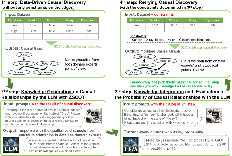
Figure 1: Overall framework of the statistical causal prompting in a large language model (LLM) and statistical causal discovery (SCD) with LLM-based background knowledge.

In addition, with respect to efficiency and precision in SCD, the importance of incorporating the constraints on trivial causal relationships into the SCD algorithms has been highlighted (Inazumi et al., 2010; Chowdhury et al., 2023). Causal learning software packages have been augmented with prior knowledge, as demonstrated in “causal-learn” , and “LiNGAM”  (Zheng et al., 2023; Ikeuchi et al., 2023).

Moreover, the systematic acquisition of the domain expert knowledge is a challenging task. Although there are several examples of constructing directed acyclic graphs (DAGs) by domain experts, as demonstrated in health services research (Rodrigues et al., 2022), practical methods for achieving the systematic construction of DAGs with domain knowledge have not been proposed.

The scenario recently has been changed with the rapid progress in the development of high-end large language models (LLMs) such as GPT-4, Gemini, and Llama. With their high performances in the applications of their domain knowledge acquired from vast amounts of data in the pre-training processes (OpenAI, 2023; Touvron et al., 2023; Gemini Team, Google, 2023), LLMs can be expected to perform objective evaluation of causal relationships. Several studies have reported the trial results of LLM knowledge-based causal inference (LLM-KBCI) (Jiang et al., 2023; Jin et al., 2023; Kıcıman et al., 2023; Zečević et al., 2023); in particular, the performance enhancement in non-parametric SCD with the guides by LLMs was confirmed (Ban et al., 2023; Vashishtha et al., 2023). However, it remains unclear whether the enhancement in SCD accuracy with background knowledge augmented by LLMs is robustly observed in inference themes involving closed data uncontained in the pre-training datasets of LLMs, and whether it leads to more statistically valid causal models.

1.2 Central Idea of Our Research

Based on the rapidly evolving prompting techniques in the context of causal inference with LLMs, a novel methodology for SCD is proposed in this paper, in which the LLM prompted with the results of SCD without background knowledge evaluates the probability of the causal relationships considering both the domain knowledge and the statistical characteristic suggested by SCD (Figure 1). In the first step, a SCD is executed on a dataset without prior knowledge, and the results of the statistical causal analysis are outputted.

In addition to the generated knowledge prompting (GKP) method, which was reported as an effective prompting technique for maximizing the usage of the expert knowledge acquired in the pre-training process of the LLM (Liu et al., 2022), the process of utilizing the LLM includes the second step (knowledge generation) and the third step (knowledge integration). In the second step, knowledge on the causal relationships between all pairs of variables is generated in detail from the domain knowledge of the LLM based on the zero-shot chain-of-thought (ZSCOT) prompting technique (Kojima et al., 2022). Here, the LLM can be prompted with the results of SCD as supplemental information for LLM inference. We define this technique as “statistical causal prompting” (SCP). Thereafter, in the third step, the LLM judges whether there are any causal relationships between all pairs of variables with “yes” or “no,” thus objectively considering the dialogs of the second step. Here, the probabilities of the responses from the LLM are evaluated, and are transformed into the prior knowledge matrix, i.e., the output of LLM-KBCI with SCP.

Finally, in the fourth step, SCD is re-applied with the PK matrix generated in the third step.

1.3 Our Contribution

The research in this paper is based on the concept proposed in Figure 1. The hypotheses are that, based on the proposed method, the output of LLM-KBCI is improved with SCP, and the final SCD result augmented with the output of LLM-KBCI is more accurate with respect to the domain expertise and statistic. Through the demonstration of the proposed method and verification of these hypotheses, the main points and contributions in this paper are as follows:

(1) Realization of the Synthesis of LLM-KBCI and SCD in a Mutually-Referential Manner

The practical method for realizing the proposed concept of Figure 1 is detailed, and the SCP method is proposed. Several experiments were demonstrated with a benchmark dataset and the disclosed data excluded from the pre-training materials of LLMs, both of which consisted of continuous variables.

(2) Mutual Performance Enhancement of the SCD and LLM-KBCI

We demonstrated that the augmentation by the LLM with SCP, improved the performance of the SCD, and the performance of LLM-KBCI was also enhanced by SCP.

(3) Enhancement of SCD Performance by SCP

In the experiments, we demonstrate the implication that the output of several SCD algorithms augmented by the LLM with SCP, can be a superior causal model t0 the pattern of prompting without SCP in terms of domain expertise and statistic, even if the dataset is biased.

2 Related Works

Augmentation of SCD Algorithms with Background Knowledge

As introduced in Section 1.1, several SCD algorithms can be systematically augmented with background knowledge. Moreover, their software packages are open. For example, as a non-parametric and constraint-based SCD method, the Peter-Clerk (PC) algorithm (Spirtes et al., 2000) is augmented with the background knowledge of the forced or forbidden directed edges in “causal-learn”. “Causal-learn” also provides the Exact Search algorithm (Silander & Myllymäki, 2006; Yuan & Malone, 2013) as a non-parametric and score-based SCD method, which can be augmented with the background knowledge of only the forbidden directed edges as a super structure matrix. Moreover, as a semi-parametric approach, DirectLiNGAM (Shimizu et al., 2011) algorithm is also augmented with prior knowledge for the causal order (Inazumi et al., 2010) in “LiNGAM” project(Ikeuchi et al., 2023).

Causal Inference in Knowledge-Driven Approach with LLMs

Since the application of LLMs is a relatively novel technology, only a few valuable trials for causal inference using LLMs have been conducted. Attempts have been made to use LLMs for causal inference among a set of variables, in addition to prompting using only the names of variables, without the SCD process with the benchmark datasets (Kıcıman et al., 2023; Zečević et al., 2023). Researches have been conducted with focus on the use of LLMs to minimize the error metrics of the score-based SCD result (Ban et al., 2023), and to improve the estimation of causal effects by the LLM decision of the causal order from triplet subgraphs, as decomposed from non-parametric SCD results (Vashishtha et al., 2023). In contrast to the studies with similar focuses on LLM-guided SCD (Ban et al., 2023; Vashishtha et al., 2023), this study focuses on the construction of the background knowledge based on the response probability of the LLM, which can reflect the credibility of the decision made by the LLM with SCP. In addition, in the case of a semi-parametric SCD method such as LiNGAM, we detail herein how to achieve both statistical validity and natural interpretation with respect to domain knowledge at a maximally high level, by prompting with the causal coefficients and bootstrap probabilities of all the patterns of directed edges.

3 Materials and Methods

3.1 Algorithms and Elements for LLM-Augmented Causal Discovery

Algorithm 1 Background knowledge construction with the LLM prompted with the results of the SCD

  Input 1: Data $X$ with variables$\{x_{1},...,x_{n}\}$

  Input 2: SCD method $S$

  Input 3: Function for bootstrap $B$

  Input 4: Response of the domain expert(GPT-4) $\epsilon_{\text{GPT4}}$

  Input 5: Log probability of the response $L(\epsilon_{\text{GPT4}})$

  Input 6: Prompt function for knowledge generation $Q_{ij}^{(1)}$

  Input 7: Prompt function for knowledge integration $Q_{ij}^{(2)}$

  Input 8: Transformation from probability matrix to prior knowledge $T$

  Input 9: Number of times to measure the probability $M$

  Output: Result of SCD with prior knowledge $\hat{G}$ on $X$

  SCD result without prior knowledge $\hat{G_{0}}=S(X)$

  bootstrap probability matrix ${\bm{P}}=B(S,X)$

  for $i=1$ to $n$ do

     for $j=1$ to $n$ do

        if $i=j$ then

           $\overline{p_{i,i}}=\text{NaN}$

        else

           prompt $q_{ij}^{(1)}=Q_{ij}^{(1)}(x_{i},x_{j},\hat{G_{0}},{\bm{P}})$

           response $a_{ij}=\epsilon_{\text{GPT4}}(q_{ij}^{(1)})$

           prompt $q_{ij}^{(2)}=Q_{ij}^{(2)}(q_{ij}^{(1)},a_{ij})$

           for $m=1$ to $M$ do

              $L_{ij}^{(m)}=L(\epsilon_{\text{GPT4}}(q_{ij}^{(2)})=\text{``yes''})$

           end for

           mean probability $\overline{p_{ij}}=\displaystyle\frac{\sum_{m=1}^{M}\exp(L_{ij}^{(m)})}{M}$

        end if

     end for

  end for

  probability matrix ${\bm{\overline{p}}}=(\overline{p_{ij}})$

  prior knowledge ${\mbox{\boldmath$PK$}}=T({\bm{\overline{p}}})$

  return $\hat{G}=S(X,{\mbox{\boldmath$PK$}})$

With respect to practicality, the method shown in Figure 1 is outlined as Algorithm 1. Following the notations in Algorithm 1, the explanation for the input elements in the demonstration is shown below, except for the Data $X$ explained in Section 3.3.

Algorithms for Statistical Causal Discovery

For the SCD method $S$, we adopted the PC algorithm (Spirtes et al., 2000), Exact Search based on the A^∗ algorithm (Yuan & Malone, 2013), and DirectLiNGAM algorithm (Shimizu et al., 2011), which can all be optionally augmented with prior knowledge and are open in “causal-learn” (Zheng et al., 2023) and “LiNGAM” (Ikeuchi et al., 2023). Furthermore, we also implement the bootstrap sampling $B$ of the SCD algorithm, to investigate the statistic properties such as the bootstrap probabilities $p_{ij}$ of the emergence of the directed edges from $x_{j}$ to $x_{i}$. In our experiments, the number of bootstrap resamplings is fixed to $1000$.

Conditions of the LLM and Prompt Engineering

For the LLM playing the role of domain expert, we adopt Chat Completion application programming interface (API) of GPT-4-1106-preview developed by OpenAI; the temperature, a hyperparameter for adjusting the probability distribution of the output from GPT-4, is fixed to $0.7$.

The template for the first prompting $q_{ij}^{(1)}$ for knowledge generation is shown in Table 1. This prompting template is composed based on the underlying principle of the ZSCOT prompting technique (Kojima et al., 2022), which was reported as a potential method to enhance the performance of the LLM generation tasks; enhancement is performed by guiding logical inference and eliciting the background knowledge acquired through the pre-training process from the LLM. Although the quality of the LLM outputs can be enhanced, e.g., by fine-tuning with several datasets containing fundamental knowledge necessary for causal inference, we adopt the idea of ZSCOT considering the necessity for establishing low-cost and simple methods, which can be universally applied independent of the targeted fields of causal inference. Furthermore, the SCD results, e.g., the causal structure and bootstrap probabilities can be included in $\langle$blank 5$\rangle$ and $\langle$blank 9$\rangle$, which are defined as “statistical causal prompting” (SCP). Since the information used in the SCP is partially dependent on the SCD algorithms, a brief description of the patterns for constructing the contents of $\langle$blank 5$\rangle$ and $\langle$blank 9$\rangle$ is presented in Section  3.2. In the experiments, we also consider the possibility that the contents in the SCP may be a critical factor that, can influence the response from GPT-4.

As shown in Table 2, generated knowledge is integrated in the second prompt, and GPT-4 is required to judge the existence of the causal effect from $x_{j}$ on $x_{i}$ from an objective point of view. Since the response from GPT-4 is required with “yes” or “no”, it is simple to quantitatively evaluate the level of GPT-4’s confidence regarding the existence of the causal relationship based on both the SCD result and domain knowledge. The probability $p_{ij}$ that GPT-4 concludes that there is a causal effect from $x_{j}$ on $x_{i}$ can be outputted by the optional function of GPT-4. Although $p_{ij}$ can be evaluated readily from the log probability of the GPT-4 response as “yes”, there is a slight fluctuation in the log probability output due to the random behavior of GPT-4. Thus, we adopt the mean probability $\overline{p_{ij}}$ of the single-shot measurement $M$ times as evidence for the background knowledge for the subsequent SCD, and we set $M=5$ in the experiments.

Table 1: Prompt template of $Q_{ij}^{(1)}(x_{i},x_{j},\hat{G_{0}},{\bm{P}})$ used for the generation of the expert knowledge of the causal effect from $x_{j}$ on $x_{i}$. The “blanks” enclosed with $\langle$ $\rangle$ are filled with description words considering the theme of the causal inference, variable names, and the algorithm name for SCD. The word for $\langle$blank 6$\rangle$ is selected from “a” or “no”, depending on the content of $\langle$blank 5$\rangle$.

Prompt Template of $q_{ij}^{(1)}=Q_{ij}^{(1)}(x_{i},x_{j},\hat{G_{0}},{\bm{P}})$
We want to carry out causal inference on $\langle$blank 1. theme$\rangle$, considering $\langle$blank 2. The description of all variables$\rangle$ as variables.
First, we have conducted the statistical causal discovery with $\langle$blank 3. The name of the SCD algorithm$\rangle$, using a fully standardized dataset on $\langle$blank 4. The description of the dataset$\rangle$.
$\langle$blank 5. Including here the information of $\hat{G_{0}}$ or ${\bm{P}}$.
The detail of the contents depends on prompting patterns.$\rangle$
According to the results shown above, it has been determined that there may be $\langle$blank 6. a/no$\rangle$ direct impact of a change in $\langle$blank 7. The name of $x_{j}$$\rangle$ on $\langle$blank 8.The name of $x_{i}$$\rangle$ $\langle$blank 9.The value of causal coefficients or bootstrap probability$\rangle$.
Then, your task is to interpret this result from a domain knowledge perspective and determine whether this statistically suggested hypothesis is plausible in the context of the domain.
Please provide an explanation that leverages your expert knowledge on the causal relationship between $\langle$blank 7. The name of $x_{j}$$\rangle$ and $\langle$blank 8. The name of $x_{i}$$\rangle$, and assess the naturalness of this causal discovery result.
Your response should consider the relevant factors and provide a reasoned explanation based on your understanding of the domain.

Table 2: Prompt template of $Q_{ij}^{(2)}(q_{ij}^{(1)},a_{ij})$ used for the quantitative evaluation of the probability of the GPT-4’s assertion that there is causal effect from $x_{j}$ on $x_{i}$.

Prompt Template of $q_{ij}^{(2)}=Q_{ij}^{(2)}(q_{ij}^{(1)},a_{ij})$
An expert was asked the question below:
$\langle$blank 10. $q_{ij}^{(1)}$$\rangle$
Then, the expert replied with its domain knowledge:
$\langle$blank 11. $a_{ij}$$\rangle$
Considering objectively this discussion above, if $\langle$blank 12. The name of $x_{j}$$\rangle$ is modified, will it have a direct or indirect impact on $\langle$blank 13. The name of $x_{i}$$\rangle$?
Please answer this question with $\langle$yes$\rangle$ or $\langle$no$\rangle$.
No answers except these two responses are needed.

Algorithm 2 Transformation from the probability matrix into the prior knowledge matrix

  Input 1: probability matrix ${\bm{p}}=(p_{ij})$

  Input 2: SCD method $S$ $S\in$ { PC, Exact Search, DirectLiNGAM }

  Output: prior knowledge matrix ${\mbox{\boldmath$PK$}}=({\mbox{$PK$}}_{ij})$

  for $i=1$ to $n$ do

     for $j=1$ to $n$ do

        if $i=j$ then

           ${\mbox{$PK$}}_{ij}=\text{Forbidden}$

        else

           if $p_{ij}<0.05$ then

              ${\mbox{$PK$}}_{ij}=\text{Forbidden}$

           else if $S=\text{Exact Search}$ then

              ${\mbox{$PK$}}_{ij}=\text{Unknown}$

           else

              if $p_{ij}\geq 0.95$ then

                 ${\mbox{$PK$}}_{ij}=\text{Forced}$

              else

                 ${\mbox{$PK$}}_{ij}=\text{Unknown}$

              end if

           end if

        end if

     end for

  end for

  if $S=\text{DirectLiNGAM}$ then

     ${\mbox{\boldmath$PK$}}=A({\mbox{\boldmath$PK$}})$ (acyclic transformation)

  end if

  return $PK$

For the subsequent SCD with prior knowledge, the probability matrix ${\bm{\overline{p}}}$ is transformed with $T$, as expressed by Algorithm 2, into the background knowledge matrix. Although we set the criteria for asserting the forced directed edge as $0.95$ and for the forbidden edge as $0.05$, the difference in the constraints which can be adopted depending on the SCD algorithms should be considered. In the Exact Search algorithm, the constraints of the forced edge cannot be applied. For the case of DirectLiNGAM, since the prior knowledge is used for the decision of the causal order in the DirectLiNGAM algorithm, the prior knowledge matrix must be an “acyclic” adjacency matrix when it is represented in the form of a network graph. Thus, when $S$ = DirectLiNGAM and $PK$ is cyclic, an additional transformation algorithm $A$ is required. In addition, there can be several acyclic transformation patterns; only one acyclic matrix with some criterion should be selected. The algorithm for the transformation and the matrix selection criterion in this study are explained in Appendix E.

3.2 Experiment Patterns of SCP

Related to the $\langle$blank 5$\rangle$ and $\langle$blank 9$\rangle$ in Table 1, we have conducted experiments in several patterns of SCP. the notations of the prompting patterns in the experiments are presented with explanations below:

Pattern 0: without SCP

This pattern corresponds to the reference for the comparison with the other patterns including SCD results in their prompts. Since the prompt template shown in Table 1 is not adequate for this pattern, we prepare a different template for Pattern 0, which is shown in Appendix B.

Pattern 1: with the list of edges that appeared in the first SCD

Directed or undirected edges between $x_{i}$ and $x_{j}$ emerged in the SCD are listed.

Pattern 2: with the list of the edges with their non-zero bootstrap probabilities

Directed or undirected edges between $x_{i}$ and $x_{j}$ that emerged once (at minimum) in the bootstrap process are listed with their bootstrap probabilities.

Pattern 3: with the list of edges that emerged in the first SCD with the calculated causal coefficients (only for DirectLiNGAM)

Based on the property of DirectLiNGAM, in that the causal coefficients are also output with the causal graph discovered in the algorithm, this pattern is also attempted in order to elucidate whether more information such as causal coefficients in addition to Pattern 1 can improve the performance of LLM-KBCI and the subsequent SCD with prior knowledge.

Pattern 4: with the list of edges with their non-zero bootstrap probabilities with the calculated causal coefficients for the full dataset (only for DirectLiNGAM)

As the pattern with the most amount of information of 1st SCD from the practical points of view, we also attempt this pattern as a mixture of Pattern 2 and 3.

3.3 Datasets for the Experiments

Although there are several widely-open benchmark datasets with well-known ground truths, particularly for Bayesian network based causal structure learning (Scutari & Denis, 2014), several of them are fully or partially composed with categorical or discrete variables. However, considering Patterns 3 and 4 for the experiments in this study, since the basic structure causal model assumes the continuous properties of all variables, it is more effective to adopt benchmark datasets fully composed with continuous variables.

Consequently, we select Deutscher Wetterdienst (DWD) climate data with six continuous variables (Mooij et al., 2016) as benchmark datasets for the experiments. Furthermore, to demonstrate that GPT-4 can aid SCD with its domain knowledge, even if the dataset used in the SCD process and analytics on the dataset are not contained in the pre-training data of GPT-4, the proposed methods are also applied on our dataset on health screening results, which has not been disclosed and therefore not learned by GPT-4. For demonstrating that the proposed methods can be applied when the dataset contains bias, which may lead to highly inaccurate SCD results, the health screening dataset for this experiment has been sampled, and we have deliberately chosen a subset where certain biases are still present. Basic information with respect to these datasets, including the first SCD results and the ground truths adopted for the evaluation, is presented in Appendix C.

4 Results and Discussions

4.1 Results in DWD Climate Data as Benchmark

For the evaluation of the experimental results, we evaluate the prior knowledge matrix $PK$ (for measuring the performance of LLM-KBCI with the prompts, including the first SCD results) and the adjacency matrix obtained in SCD with $PK$ for each pattern (for measuring the performance of SCD augmented with LLM-KBCI), with the structural hamming distance (SHD), false positive rate (FPR), false negative rate (FNR), precision, and F1 score, using the ground truth adjacency matrix $GT$ as a reference. In addition, this paper presents a discussion on the knowledge-based matching and evaluation of the comparative fit index (CFI) (Bentler, 1990), root mean square error of approximation (RMSEA) (Steiger & Lind, 1980) and Bayes information criterion (BIC) (Schwarz, 1978) of the causal structure obtained in SCD with $PK$, under the assumption of linear Gaussian data; this is done to evaluate the results with respect to the statistical validity of calculated causal models. The list of the indices for all patterns on the DWD climate dataset are summarized in Table 3, and the results on other benchmark datasets, which exhibit almost similar behaviors to those of DWD data detailed in Appendix G.

Table 3: Comparison of the SCD results (and structural familiarity of $PK$ with ground truths, for the evaluation of the performance of LLM-KBCI) in all the experiment patterns applied to DWD climate data. Lower values are superior for SHD, FPR, FNR, RMSEA and BIC, and higher values for precision, F1score and CFI. Several outputs of LLM-KBCI and those of SCD for the cases of Exact Search and DirectLiNGAM in Patterns 1–4 (with SCP) may be a superior causal model to Pattern 0.

SCD algorithm	Pattern	SHD	FPR	FNR	Precision	F1score	CFI	RMSEA	BIC
PC	wo $PK$	9	0.20	0.83	0.14	0.15	0.90	0.22	69.32
	Pattern 0	5 (8)	0.03 (0.20)	0.67 (0.33)	0.67 (0.40)	0.44 (0.50)	0.71	0.36	32.70
	Pattern 1	5 (9)	0.03 (0.23)	0.67 (0.33)	0.67 (0.36)	0.44 (0.47)	0.71	0.36	32.70
	Pattern 2	5 (8)	0.03 (0.20)	0.67 (0.33)	0.67 (0.40)	0.44 (0.50)	0.71	0.36	32.70
Exact Search	wo $PK$	6	0.20	0.17	0.45	0.59	0.91	0.28	92.87
	Pattern 0	5 (8)	0.10 (0.20)	0.33 (0.33)	0.57 (0.40)	0.62 (0.50)	0.98	0.12	58.38
	Pattern 1	5 (5)	0.10 (0.13)	0.33 (0.17)	0.57 (0.56)	0.62 (0.67)	0.91	0.19	57.73
	Pattern 2	6 (9)	0.13 (0.23)	0.33 (0.33)	0.50 (0.36)	0.57 (0.47)	0.91	0.20	63.58
DirectLiNGAM	wo $PK$	10	0.33	0.67	0.17	0.22	1.00	0.00	99.53
	Pattern 0	4 (8)	0.07 (0.20)	0.33 (0.33)	0.67 (0.40)	0.67 (0.50)	1.00	0.00	52.67
	Pattern 1	8 (8)	0.10 (0.10)	0.83 (0.83)	0.25 (0.25)	0.20 (0.20)	0.64	0.43	38.03
	Pattern 2	4 (7)	0.03 (0.17)	0.50 (0.33)	0.75 (0.44)	0.60 (0.53)	0.98	0.09	40.80
	Pattern 3	5 (6)	0.10 (0.13)	0.33 (0.33)	0.57 (0.50)	0.62 (0.57)	0.93	0.16	57.90
	Pattern 4	5 (6)	0.10 (0.17)	0.33 (0.16)	0.57 (0.50)	0.62 (0.62)	0.92	0.18	57.80

Enhancing the performance with prior knowledge augmentation by GPT-4

One of the characteristics presented in Table 3 is as follows: the result of SCD augmented with $PK$ is more similar to $GT$ than the first SCD result without prior knowledge. This behavior is interpreted as the knowledge-based improvement of the causal graph by GPT-4 as a domain expert, which is qualitatively consistent with other related works on LLM-guided causal inference (Ban et al., 2023; Vashishtha et al., 2023). Moreover, the metrics of the precision or F1 score are higher after the SCD is augmented with $PK$ than the pure $PK$, which are conclusions of LLM-KBCI using GPT-4. This comparison results suggest that even if LLM-KBCI is not optimal, the ground truth can be better approached, by conducting SCD augmented with LLM-KBCI. In addition, BIC decreases in almost all the patterns from the SCD result without $PK$. The aforementioned properties suggest that knowledge-based augmentation from GPT-4 can improve the precision of SCD in terms of the consistency with respect to the domain expert knowledge and statistical causal structure.

Prompting pattern dependence of the performance of LLM-KBCI and SCD with prior knowledge

Moreover, in multiple cases, the precision and F1 score of $PK$ generated from Pattern 0 are smaller than several of the other patterns, in which GPT-4 has undergone SCP. This supports the performance enhancement of LLM-KBCI by SCP.

On the other hand, the output of the SCD augmented with $PK$, Pattern 0 stably indicates a relatively higher performance among all the patterns in terms of domain knowledge and statistical model fitting. In particular, the results of Patterns 0 and 1 are almost the same when the PC or the Exact Search algorithm is adopted. The scenario differs when we use the DirectLiNGAM algorithm. The quality of the result from DirectLiNGAM with SCP in Pattern 2 is superior to that of Pattern 0 in terms of FPR, precision and BIC, although other parameters in Pattern 2 are comparable or inferior to those in Pattern 0. This implies that SCP for the knowledge generation process in GPT-4, can effectively improve the performance of DirectLiNGAM.

However, from the analysis of Patterns 3 and 4, in which GPT-4 is prompted with the causal coefficients of the first SCD results, it is revealed that prompting with a greater amount of statistical information does not always lead to improved SCD results. In particular, while $PK$ in Pattern 4 is closer to the ground truth matrix than that in Pattern 0, the final SCD result augmented with $PK$ in Pattern 4 is inferior to that of Pattern 0.

4.2 Results in Randomly Selected Sub-sample of Health Screening Data Excluded from GPT-4 Pre-Training Dataset

To confirm the practical use of the proposed method, including the scenario wherein the range of the available dataset for statistical causal inference is limited to observation data, which may be statistically biased, and the trivial causal relationships are not appearent in SCD without prior knowledge, we also apply the proposed methods on the sub-dataset of health screening results, which has been randomly sampled from the entire dataset, and the natural ground truth is not presented in SCD results without $PK$.

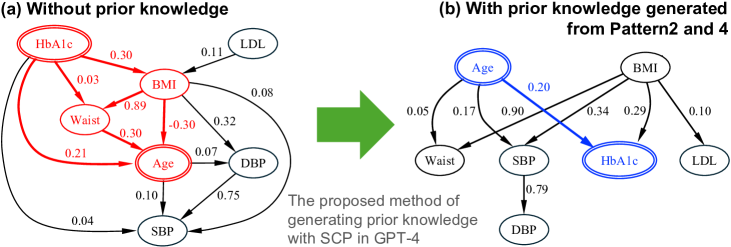
Figure 2: Results of DirectLiNGAM in the health screening data. (a) Result without prior knowledge. (b) Result with prior knowledge, which is generated from GPT-4 with SCP in Patterns 2 and 4. In this randomly selected subset, the DirectLiNGAM result without prior knowledge exhibits unnatural paths drawn in red in (a), which indicates that “Age” is influenced by “HbA1c”. However, using the proposed method, the unnatural behavior is clearly mitigated with the guide of prior knowledge generated from GPT-4 with SCP, including the value of causal coefficients in (a) or the bootstrap probabilities of causal relationships between pairs of variables.

In Figure 2(a), the result of DirectLiNGAM without $PK$ is shown, and unnatural directed edges to “Age” from other variables are suggested, although the parts of the ground truths from expert knowledge are reversed relationships from these edges, such as “Age”$\rightarrow$“HbA1c”. However, when the causal discovery is assisted with $PK$ generated from GPT-4 with SCP in Patterns 2 and 4, the causal graph becomes more natural: “Age” is not influenced by other variables, and the ground truth “Age”$\rightarrow$“HbA1c”, which cannot be detected without $PK$ in this randomly selected subset, appears in the causal graph, as shown in Figure 2(b). Since this sub-dataset and the analysis results are not disclosed and have been completely excluded from the pre-training data for GPT-4, GPT-4 cannot respond to prompts asking for the causal relationships merely by reproducing the knowledge acquired from the same data. Based on the above, it is verified that the assist of GPT-4 with SCP can cause the result of SCD to further approach the ground truths to an extent, even when the dataset is not learned by GPT-4 and contains bias.

Table 4: Characteristic results of causal discovery in the proposed methods on the subset of health screening data with certain biases.
A: The elements of $\bm{P}$ generated in each prompting pattern for all the appropriate ground truth causal relationships in these variables. The values enclosed in parentheses are the bootstrap probabilities of the directed edges in the DirectLiNGAM algorithm without $PK$. Moreover, all the probabilities of reversed, unnatural causal relationships in which “age” is influenced by other factors are extremely closed to zero. B: CFI, RMSEA and BIC evaluated on the model fitting with the structure discovered by DirectLiNGAM, under the assumption of linear-Gaussian data. The values enclosed in parentheses are the statistics of the structure calculated without $PK$. It can be inferred that SCP with the inclusion of bootstrap probabilities in such as those in Patterns 2 and 4, have enhanced the confidence in “Age”$\rightarrow$“DBP” by GPT-4, and improved the BIC of linear-Gaussian fitting with the structures in DirectLiNGAM with $PK$ when compared with Pattern 0.

		Pattern 0	Pattern 1	Pattern 2	Pattern 3	Pattern 4
A. Probability of reproducing ground truth from GPT-4	“Age”$\rightarrow$“BMI” (0.166)	0.901	0.076	0.093	0.306	0.037
	“Age”$\rightarrow$“SBP” (0.550)	0.626	0.302	0.207	0.235	0.795
	“Age”$\rightarrow$“DBP” (0.308)	0.001	0.019	0.115	0.095	0.926
	“Age”$\rightarrow$“HbA1c” (0.327)	0.986	0.170	0.723	0.046	0.176
B. Statistics of linear-Gaussian fitting with the results of DirectLiNGAM	CFI (1.002)	0.999	0.992	0.995	0.986	0.995
	RMSEA (0.000)	0.018	0.054	0.032	0.057	0.032
	BIC (124.332)	103.581	89.738	89.740	103.506	89.740

For further clarity regarding the behaviors of SCP, the mean probabilities of the positive response on the causal relationships from GPT-4 for ground truths in the health screening data, in additon to the statistics of the fitting results with the structure suggested by DirectLiNGAM with SCP are presented in Table 4. In Pattern 0 without SCP, the existence of “Age”$\rightarrow$“BMI” and “Age”$\rightarrow$“HbA1c” is supported in the probabilities over $0.90$, and the probabilities decrease in other patterns with SCP. On the other hand, the opposite behavior is also observed on “Age”$\rightarrow$“DBP”, which is strongly denied from the GPT-4 domain knowledge without SCP in Pattern 0. It is reasonable to interpret that these probability changes with SCP in GPT-4 are induced by the results of SCD and bootstrap probabilities included in the promptings.

For example, focusing on the relationship “Age”$\rightarrow$“BMI”, the lack of the direct edge in the SCD result with $PK$ shown in Figure 2(a) and the relatively low bootstrap probability $0.166$ in Table 4, may be the cause of lower probability in the SCP patterns than Pattern 0. In contrast, although the hypothesis of “Age”$\rightarrow$“DBP” is not supported by the GPT-4 domain knowledge in Pattern 0, the appearance of the edge in Figure 2(a) and the bootstrap probability $0.308$ are considered to be the cause of the increase in probability through SCP. Considering the aforementioned properties, the probability that the judgement rendered by GPT-4 regarding causal relationships can be influenced by the SCD results, particularly when the dataset with some significant biases is used in the causal discovery.

Finally, it is also confirmed that the BIC becomes smaller with the assistance by GPT-4 than without $PK$. In particular, the values in Patterns 1, 2 and 4 are lower than Pattern 0. This suggests that SCP can contribute to the discovery of the causal structure with more adequate statistical models.

5 Conclusion

In this study, a novel methodology of causal inference, in which SCD and LLM-KBCI are synthesized with SCP and prior knowledge augmentation has been developed and demonstrated.

It has been revealed that GPT-4 can cause the output of LLM-KBCI and the SCD result with prior knowledge from LLM-KBCI to approach the ground truth, and that the SCD result can be further improved, if GPT-4 undergoes SCP. Furthermore, we have demonstrated that GPT-4 with SCP can assist in SCD with respect to domain expertise and statistics, and that the proposed method is effective even if the sample size is not sufficiently large to obtain reasonable SCD results.

For the practical application of the proposed method, further basic research on the effect of causal coefficients or bootstrap probabilities on the results of LLM-KBCI is required.

6 Impact statement

This paper proposes a novel approach that integrates SCD methods with LLMs. This research has the potential to contribute to more accurate causal inference in fields where understanding causality is crucial, such as healthcare, economics, and environmental science. However, the use of LLMs such as GPT-4 necessitates the extensive consideration of data privacy and biases. This study highlights the responsible use of artificial intelligence (AI), considering ethical implications and societal impacts. With appropriate guidelines and ethical standards, the proposed methodology can advance scientific understanding and provide extensive widespread benefits to society.

7 Acknowledgements

We sincerely appreciate Dr. Hitoshi Koshiba for his invaluable assistance in shaping the overall structure of this paper and for engaging in fruitful discussions. We would like to thank Editage for English language editing. This work was supported by the Japan Science and Technology Agency (JST) under CREST Grant Number JPMJCR22D2 and PRESTO Grant Number JPMJPR2123, and by the Japan Society for the Promotion of Science (JSPS) under KAKENHI Grant Numbers JP20K03743 and JP23H04484.

Appendix A Ethics Review

Ethical Considerations in Methodology and AI Use

This paper proposes a novel approach that integrates SCD with LLMs. We have thoroughly considered the issues of data privacy and biases associated with the use of LLMs. The proposed methodology enhances the accuracy and efficiency of causal discovery; however, it does not introduce explicit ethical implications beyond those generally applicable to machine learning. We are committed to the responsible use of AI and welcome the scrutiny of the ethics review committee.

Institutional Review and Consent Compliance of Health Screening Data

The institutional review board of Kyoto University approved this study. As we only analyzed anonymized data from the database, the need for informed consent was waived.

Appendix B Detail of Contents in Each Prompting Pattern

In this section, the details of the prompting in each pattern are presented. For Pattern 0, another prompting template is detailed instead of the sentences shown in Table 1. Moreover, for Patterns 1, 2, 3 and 4, the contents filled in $\langle$blank 5$\rangle$ and $\langle$blank 9$\rangle$ of the prompt template for SCP shown in Table 1 are described.

For Pattern 0

Compared with other patterns of SCP, Pattern 0 does not include the any results of SCD without prior knowledge. As a result, the prompt template in Table 1 is not suitable for Pattern 0, as it includes the blanks filled with the description of the dataset and SCD result. Thus, we prepare another prompt template for Pattern 0, which is completely independent of the SCD result and require GPT-4 to generate the response solely from its domain knowledge. Table 5 presents the prompt template in Pattern 0, which is composed mainly from the ZSCOT concept. Since it does not include information on the SCD method and relies solely on the domain knowledge in GPT-4, the probability matrix from the process of GPT-4 in Pattern 0 is applied independently of the SCD method.

Table 5: The prompt template of $Q_{ij}^{(1)}(x_{i},x_{j})$ for Pattern 0 for the generation of the expert knowledge of the causal effect from $x_{j}$ on $x_{i}$. The “blanks” enclosed with $\langle$ $\rangle$ are filled with description words of the theme of the causal inference and variable names.

Prompt Template of $q_{ij}^{(1)}=Q_{ij}^{(1)}(x_{i},x_{j})$ in Pattern 0 (for all SCD methods)
We want to carry out causal inference on $\langle$blank 1. theme$\rangle$, considering $\langle$blank 2. The description of all variables$\rangle$ as variables.
If $\langle$blank 7. The name of $x_{j}$$\rangle$ is modified, will it have a direct impact on $\langle$blank 8.The name of $x_{i}$$\rangle$?
Please provide an explanation that leverages your expert knowledge on the causal relationship between $\langle$blank 7. The name of $x_{j}$$\rangle$ and $\langle$blank 8. The name of $x_{i}$$\rangle$.
Your response should consider the relevant factors and provide a reasoned explanation based on your understanding of the domain.

For Patterns 1–4 (in the case of Exact Search and DirectLiNGAM)

Following the concept of each SCP pattern, the contents filled in $\langle$blank 5$\rangle$ shown in Table 1 are summarized in Table 7. In this table, the names of the causes and effected variables are represented as $\langle$ cause $i$ $\rangle$ and $\langle$ effect $i$ $\rangle$ respectively, and the bootstrap probability of this causal relationship in SCD $P_{i}$ and the causal coefficient of LiNGAM $b_{i}$ can be included in Patterns 2–4. In Patterns 2 and 4, only the causal relationships with $P_{i}\neq 0$ are listed in $\langle$ blank 5 $\rangle$. In Pattern 3, the causal relationships with $b_{i}\neq 0$ are listed in $\langle$ blank 5 $\rangle$. The contents filled in $\langle$blank 6$\rangle$ and $\langle$blank 9$\rangle$ also depend on the SCP patterns, and are shown in Table 7. Here, we define the bootstrap probability of $x_{j}\rightarrow x_{i}$ as $P_{ij}$. we also define the causal coefficient of $x_{j}\rightarrow x_{i}$ in LiNGAM as $b_{ij}$, since the structural equation of LiNGAM is usually defined as:

$$x_{i}=\sum_{i\neq j}b_{ij}x_{j}+e_{i}$$ (1)

Table 6: Contents filled in $\langle$blank 5$\rangle$ shown in Table 1, when Exact Search or DirectLiNGAM is adopted for the SCD process.

SCP Pattern	Content in $\langle$blank 5$\rangle$
Pattern 1 Directed edges	All of the edges suggested by the statistical causal discovery are below: $\langle$ cause 1 $\rangle$ $\rightarrow$ $\langle$ effect 1 $\rangle$ $\langle$ cause 2 $\rangle$ $\rightarrow$ $\langle$ effect 2 $\rangle$ ⋮
Pattern 2 Bootstrap probabilities of directed edges	All of the edges with non-zero bootstrap probabilities suggested by the statistical causal discovery are below: $\langle$ cause 1 $\rangle$ $\rightarrow$ $\langle$ effect 1 $\rangle$ (bootstrap probability = $P_{1}$) $\langle$ cause 2 $\rangle$ $\rightarrow$ $\langle$ effect 2 $\rangle$ (bootstrap probability = $P_{2}$) ⋮
Pattern 3 (DirectLiNGAM Only) Non-zero causal coefficients of directed edges	All of the edges and their coefficients of the structural causal model suggested by the statistical causal discovery are below: $\langle$ cause 1 $\rangle$ $\rightarrow$ $\langle$ effect 1 $\rangle$ (coefficient = $b_{1}$) $\langle$ cause 2 $\rangle$ $\rightarrow$ $\langle$ effect 2 $\rangle$ (coefficient = $b_{2}$) ⋮
Pattern 4 (DirectLiNGAM Only) Non-zero causal coefficients and bootstrap probabilities of directed edges	All of the edges with non-zero bootstrap probabilities and their coefficients of the structural causal model suggested by the statistical causal discovery are below: $\langle$ cause 1 $\rangle$ $\rightarrow$ $\langle$ effect 1 $\rangle$ (coefficient = $b_{1}$, bootstrap probability = $P_{1}$) $\langle$ cause 2 $\rangle$ $\rightarrow$ $\langle$ effect 2 $\rangle$ (coefficient = $b_{2}$, bootstrap probability = $P_{2}$) ⋮

Table 7: Contents filled in $\langle$blank 6$\rangle$ and $\langle$blank 9$\rangle$ shown in Table 1, when Exact Search or DirectLiNGAM is adopted for the SCD process.

SCP Pattern	Case Classification	$\langle$blank 6$\rangle$	Content in $\langle$blank 9$\rangle$
Pattern 1 Directed edges	$x_{j}\rightarrow x_{i}$ emerged	a	- (No values are filled in)
	$x_{j}\rightarrow x_{i}$ not emerged	no	- (No values are filled in)
Pattern 2 Bootstrap probabilities of directed edges	$P_{ij}\neq 0$	a	with a bootstrap probability of $P_{ij}$
	$P_{ij}=0$	no	- (No values are filled in)
Pattern 3 (DirectLiNGAM Only) Non-zero causal coefficients of directed edges	$b_{ij}\neq 0$	a	with a causal coefficient of $b_{ij}$
	$b_{ij}=0$	no	- (No values are filled in)
Pattern 4 (DirectLiNGAM Only) Non-zero causal coefficients and bootstrap probabilities of directed edges	$P_{ij}\neq 0$ and $b_{ij}\neq 0$	a	with a bootstrap probability of $P_{ij}$, and the coefficient is likely to be $b_{ij}$
	$P_{ij}\neq 0$ and $b_{ij}=0$	a	with a bootstrap probability of $P_{ij}$, but the coefficient is likely to be 0
	$P_{ij}=0$	no	- (No values are filled in)

Prompt Template in case of PC algorithm

Although the causal relationships are ultimately represented only as directed edges in Exact Search and DirectLiNGAM, the situation changes slightly when we adopt the PC algorithm along with the codes in “causal-learn”. This is because the PC algorithm can also output undirected edges, when the causal direction between a pair of variables cannot be determined. Therefore, we have tenteatively decided to include not only directed edges but also undirected edges in SCP. Additionally, we have prepared another prompting template for SCP in the case of PC, as shown in Table 8. This template is slightly modified from the one in Table 1. The description for $\langle$ blank 5 $\rangle$ in each SCP pattern is augmented by Table 10, and the description for $\langle$ blank 6 $\rangle$ is similarly augmented by Table 10.

As shown in Table 10, the directed and undirected edges are separately listed and clearly distinguished by the edge symbols of “$\rightarrow$” for directed edges and “—” for undirected edges. These are then filled in $\langle$ blank 5 $\rangle$. The pairs of variables connected by undirected edges are represented as $\langle$ cause or effect $i$-1 $\rangle$ and $\langle$ cause or effect $i$-2 $\rangle$, and the bootstrap probability of the emergence of these relationships is represented as $P_{i}^{u}$. On the other hand, the bootstrap probability of $\langle$ cause $i$ $\rangle$ $\rightarrow$ $\langle$ effect $i$ $\rangle$ is represented as $P_{i}^{d}$.

The Division of the descriptions in $\langle$ blank 6 $\rangle$ is shown in Table 10. The bootstrap probabilities of the appearance of $x_{j}\rightarrow x_{i}$ and $x_{j}$—$x_{i}$ are respectively represented as $P_{ij}^{d}$ and $P_{ij}^{u}$.

Table 8: The prompt template of $Q_{ij}^{(1)}(x_{i},x_{j},\hat{G_{0}},\bm{P^{d}},\bm{P^{u}})$ in case of the PC algorithm. The “blanks” enclosed with $\langle$ $\rangle$ are filled with description words considering the theme of the causal inference, variable names, and the SCD result with the PC algorithm.

Prompt Template of $q_{ij}^{(1)}=Q_{ij}^{(1)}(x_{i},x_{j},\hat{G_{0}},\bm{P^{d}},\bm{P^{u}})$ for PC
We want to carry out causal inference on $\langle$blank 1. theme$\rangle$, considering $\langle$blank 2. The description of all variables$\rangle$ as variables.
First, we have conducted the statistical causal discovery with PC (Peter-Clerk) algorithm, using a fully standardized dataset on $\langle$blank 4. The description of the dataset$\rangle$.
$\langle$blank 5. Including here the information of $\hat{G_{0}}$ (for Pattern 1), or $\bm{P^{d}}$ and $\bm{P^{u}}$ (for Pattern 2).
The detail of the contents depends on prompting patterns, both for directed and undirected edges.$\rangle$
According to the results shown above, it has been determined that
$\langle$blank 6. detail of the interpretation on whether there is a causal relationship between $x_{j}$ and $x_{i}$ from the result shown in blank 5$\rangle$.
Then, your task is to interpret this result from a domain knowledge perspective and determine whether this statistically suggested hypothesis is plausible in the context of the domain.
Please provide an explanation that leverages your expert knowledge on the causal relationship between $\langle$blank 7. The name of $x_{j}$$\rangle$ and $\langle$blank 8. The name of $x_{i}$$\rangle$, and assess the naturalness of this causal discovery result.
Your response should consider the relevant factors and provide a reasoned explanation based on your understanding of the domain.

Table 9: Contents filled in $\langle$blank 5$\rangle$ shown in Table 8.

SCP Pattern	Content in $\langle$blank 5$\rangle$
Pattern 1 Directed and undirected edges	All of the edges suggested by the statistical causal discovery are below: $\langle$ cause 1 $\rangle$ $\rightarrow$ $\langle$ effect 1 $\rangle$ $\langle$ cause 2 $\rangle$ $\rightarrow$ $\langle$ effect 2 $\rangle$ ⋮ In addition to the directed edges above, all of the undirected edges suggested by the statistical causal discovery are below: $\langle$ cause or effect 1-1 $\rangle$ — $\langle$ cause or effect 1-2 $\rangle$ $\langle$ cause or effect 2-1 $\rangle$ — $\langle$ cause or effect 2-2 $\rangle$ ⋮
Pattern 2 Bootstrap probabilities of directed and undirected edges	All of the edges with non-zero bootstrap probabilities suggested by the statistical causal discovery are below: $\langle$ cause 1 $\rangle$ $\rightarrow$ $\langle$ effect 1 $\rangle$ (bootstrap probability = $P_{1}^{d}$) $\langle$ cause 2 $\rangle$ $\rightarrow$ $\langle$ effect 2 $\rangle$ (bootstrap probability = $P_{2}^{d}$) ⋮ In addition to the directed edges above, all of the undirected edges suggested by the statistical causal discovery are below: $\langle$ cause or effect 1-1 $\rangle$ — $\langle$ cause or effect 1-1 $\rangle$ (bootstrap probability = $P_{1}^{u}$) $\langle$ cause or effect 2-1 $\rangle$ — $\langle$ cause or effect 2-2 $\rangle$ (bootstrap probability = $P_{2}^{u}$) ⋮

Table 10: Contents filled in $\langle$blank 6$\rangle$ shown in Table 8.

SCP Pattern	Case Classification	Content in $\langle$blank 6$\rangle$
Pattern 1 Directed and undirected edges	$x_{j}\rightarrow x_{i}$	there may be a direct impact of a change in $\langle$blank 7. name of $x_{j}$$\rangle$ on $\langle$blank 8. name of $x_{i}$$\rangle$
	$x_{j}$ — $x_{i}$	there may be a direct causal relationship between $\langle$blank 7. name of $x_{j}$$\rangle$ and $\langle$blank 8. name of $x_{i}$$\rangle$, although the direction has not been determined
	no edge between $x_{i}$ and $x_{j}$	there may be no direct impact of a change in $\langle$blank 7. name of $x_{j}$$\rangle$ on $\langle$blank 8. name of $x_{i}$$\rangle$
Pattern 2 Bootstrap probabilities of directed and undirected edges	$P_{ij}^{d}\neq 0$ and $P_{ij}^{u}\neq 0$	there may be a direct impact of a change in $\langle$blank 7. name of $x_{j}$$\rangle$ on $\langle$blank 8. name of $x_{i}$$\rangle$ with a bootstrap probability of $P_{ij}^{d}$. In addition, it has also been shown above that there may be a direct causal relationship between $\langle$blank 7. name of $x_{j}$$\rangle$ and $\langle$blank 8. name of $x_{i}$$\rangle$ with a bootstrap probability of $P_{ij}^{u}$, although the direction has not been determined
	$P_{ij}^{d}\neq 0$ and $P_{ij}^{u}=0$	there may be a direct impact of a change in $\langle$blank 7. name of $x_{j}$$\rangle$ on $\langle$blank 8. name of $x_{i}$$\rangle$ with a bootstrap probability of $P_{ij}^{d}$
	$P_{ij}^{d}=0$ and $P_{ij}^{u}\neq 0$	there may be a direct causal relationship between $\langle$blank 7. name of $x_{j}$$\rangle$ and $\langle$blank 8. name of $x_{i}$$\rangle$ with a bootstrap probability of $P_{ij}^{u}$, although the direction has not been determined
	$P_{ij}^{d}=0$ and $P_{ij}^{u}=0$	there may be no direct impact of a change in $\langle$blank 7. name of $x_{j}$$\rangle$ on $\langle$blank 8. name of $x_{i}$$\rangle$

Appendix C Details of Datasets used in Demonstrations

In this section, the details of the dataset used in the main body and the appendix are clarified. The ground truths set for the evaluation of the SCD and LLM-KBCI results for each dataset are presented.

C.1 Auto MPG data

Auto MPG data was originally open in the UCI Machine Learning Repository (Quinlan, 1993), and used as a benchmark dataset for causal inference (Spirtes et al., 2010; Mooij et al., 2016). It consists of the variables around the fuel consumption of cars. We adopt five variables: “Weight”, “Displacement”, “Horsepower”, “Acceleration” and “Mpg”(miles per gallon). Moreover, the number of the points of this dataset in the experiment is $392$. The ground truth of causal relationships we adopt in this paper is shown in Figure 3; the original has been shown as the example of kPC algorithm (Spirtes et al., 2010). The differences from the original study (Spirtes et al., 2010) are presented below:

(1) Loss of “Cylinders”

Although there is also a discrete variable of “Cylinders” in the original data (Quinlan, 1993), it is omitted in the experiments to focus solely on the continuous variables.

(2) Directed edge from “Weight” to “Displacement”

The “Weight” and “Displacement” are connected with an undirected edge, which indicates that the direction cannot be determined in the kPC algorithm, although a causal relationship between these two variables is suggested. However,it is empirically acknowledge that for large and heavy vehicles to use engines with larger displacement to provide sufficient power to match their size. Thus, we temporally set the direction of the edge between these two variable as “Weight” $\rightarrow$ “Displacement”.

We also recognize that another ground truth was interpreted in the process of reconstructing the Tübingen database for causal-effect pairs (Mooij et al., 2016) , and “Mpg” and “Acceleration” were interpreted as effected variables from other elements. This ground truth seems to be reliable, if we do not significantly discriminate between direct and indirect causal effects and targeting the identification of cause and effect from a pair of variables. However, we adopt the ground truth based on the result from kPC algorithm, since our target is to approach the true causal graph, including multi-step causal relationships.

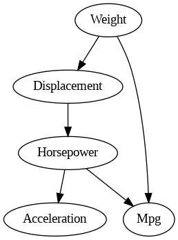
Figure 3: Causal graph of ground truth adopted for Auto MPG data in this study.

In Figure 4, the results of basic causal structure analysis by the PC, Exact Search, and DirectLiNGAM algorithms without prior knowledge are presented. Several reversed edges from ground truths such as “Mpg” $\rightarrow$ “Weight” are observed.

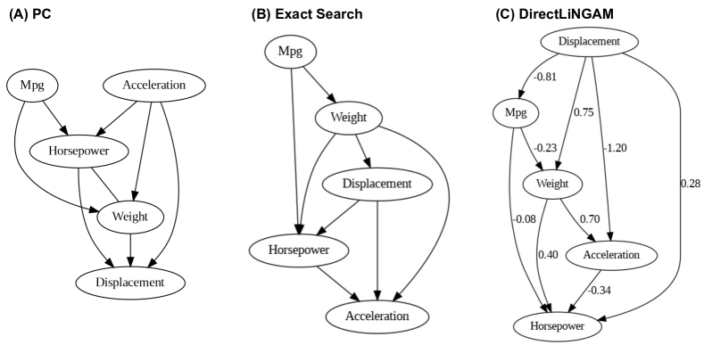
Figure 4: Results of SCD on Auto MPG data with (A) PC, (B) Exact Search, and (C) DirectLiNGAM.

C.2 DWD climate data

The DWD climate data was originally provided by the DWD , and several of the original datasets were merged and reconstructed as a component of the übingen database for causal-effect pairs (Mooij et al., 2016). It consists of six variables: “Altitude”, “Latitude”, “Longitude”, “Sunshine” (duration), “Temperature” and “Precipitation”. The number of points of this dataset is $349$, which corresponds to the number of the weather stations in Germany without missing data.

Since there is no ground truth on this dataset advocated, except for that in the übingen database for causal-effect pairs (Mooij et al., 2016), we adopt it temporally in this experiment, as shown in Figure 5.

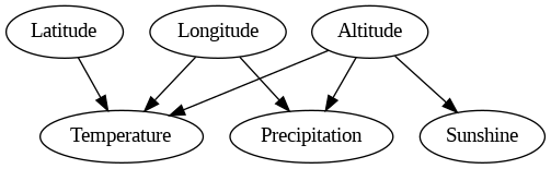
Figure 5: Causal graph of ground truth adopted for DWD climate data in this study.

In Figure 6, the results of basic causal structure analysis by the PC, Exact Search, and DirectLiNGAM algorithms without prior knowledge are presented. In all the causal graphs in Figure 6, several unnatural behaviors are observed, such as “Altitude” being effected by other climate variables, which we interpret as reversed causal relationships from the ground truths.

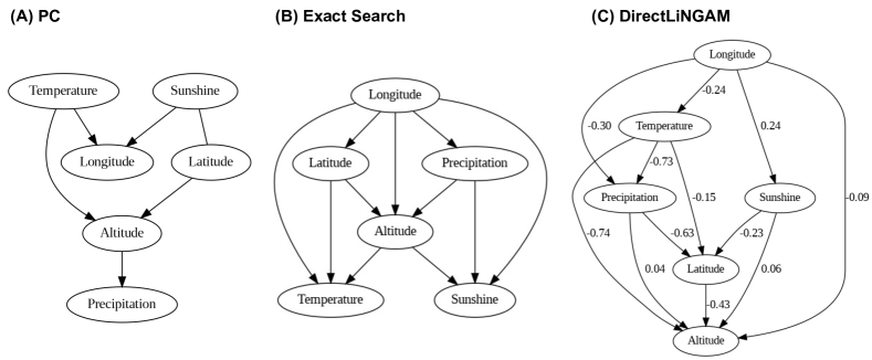
Figure 6: Results of SCD on DWD climate data with (A) PC, (B) Exact Search, and (C) DirectLiNGAM.

C.3 Sachs protein data

This dataset consists of the variables of the phosphorylation level of proteins and lipids in primary human immune cells, which were originally constructed and analyzed with the non-parametric causal structure learning algorithm by Sachs et al. (Sachs et al., 2005). It contains 11 continuous variables: “raf”, “mek”, “plc”, “pip2”, “pip3”, “erk”, “akt”, “pka”, “pkc”, “p38” and “jnk”. The number of points of this dataset is $7466$.

The ground truth adopted in this study is almost the same as the interpretation shown in the study by Sachs et al. (Sachs et al., 2005). The differences from the causal graph visually displayed in the original paper are presented below:

(1) Reversed edge between “pip3” and “plc”

Although the directed edge “plc” $\rightarrow$ “pip3” was detected in the original study, it was denoted as “reversed”, which may be the reversed direction from the expected edge. Thus, we adopt the causal relationship of “pip3” $\rightarrow$ “plc”, which Sachs et al. anticipated as true from an expert point of view.

(2) Three missed edges in the original study

In the study by Sachs et al., “pip2” $\rightarrow$ “pkc”, “plc” $\rightarrow$ “pkc” and “pip3” $\rightarrow$ “akt” did not appear in the Bayesian network inference result, although they were expected to be direct causal relationships from the domain knowledge. We adopt these three edges for the ground truth considering that they may not appear under certain SCD conditions and assumptions.

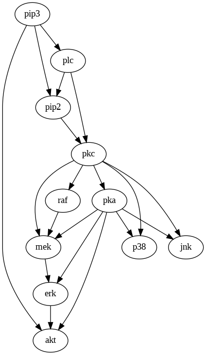
Figure 7: Causal graph of ground truth adopted for Sachs protein data in this study.

In Figure 8, the results of the basic causal structure analysis by the PC, Exact Search, and DirectLiNGAM algorithms without prior knowledge are shown.

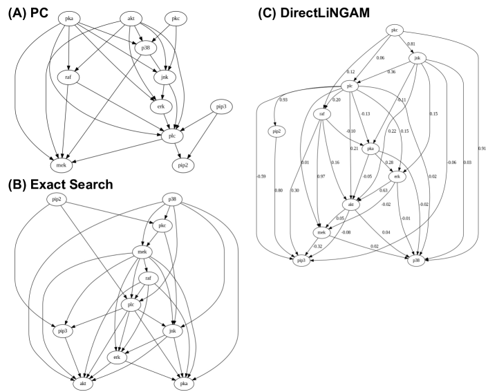
Figure 8: Results of SCD on Sachs data with (A) PC, (B) Exact Search, and (C) DirectLiNGAM.

C.4 Health screening data (closed data and not included in GPT-4’s pre-training materials)

To confirm that GPT-4 can adequately judge the existence of causal relationships with SCP, even if the dataset used in SCD is not included in the pre-training dataset of GPT-4, we have additionally prepared the health screening dataset of workers in engineering and construction contractors, which is not disclosed due to its sensitive nature from personal handling and other private aspects. It contains seven continuous variables: body mass index (“BMI”), waist circumference (“Waist”), Systolic blood pressure (“SBP”), Diastolic blood pressure (“DBP”), hemoglobin A1c (“HbA1c”), low density lipoprotein cholesterol (“LDL”), and age (“Age”). The number of total points of this dataset is $123\,151$.

Although the causal relationships between all pairs of variables are not completely determined, we set two types of ground truths.

(1) Directed edges interpreted as ground truths

We emprically set four directed edges below as ground truths.

• “Age”$\rightarrow$“BMI”(Clarke et al., 2008; Alley et al., 2008; Gordon-Larsen et al., 2010; Yang et al., 2021)

• at least one of “Age”$\rightarrow$“SBP” and “Age”$\rightarrow$“DBP”(Gurven et al., 2012)

• “Age”$\rightarrow$“HbA1c”(Pani et al., 2008; RaviKumar et al., 2011; Dubowitz et al., 2014)

(2) Variable interpreted as a parent for all other variables

“Age” is an unmodifiable background factor. Furthermore, it has been clearly demonstrated in numerous medical studies that aging affects “BMI”, “SBP, “DBP”, and “HBA1c”. Based on this specialized knowledge, we interpret “Age” is a parent for all other variables.

The ground truths introduced above also appears in the result of DirectLiNGAM without prior knowledge, as shown in Figure 9. Although “Age”$\rightarrow$“HbA1c” is confirmed in this result, the causal coefficient of this edge is relatively small. Thus, depending on the number of the data points or the bias of the dataset, it is possible that this edge does not appear in all SCD methods without prior knowledge.

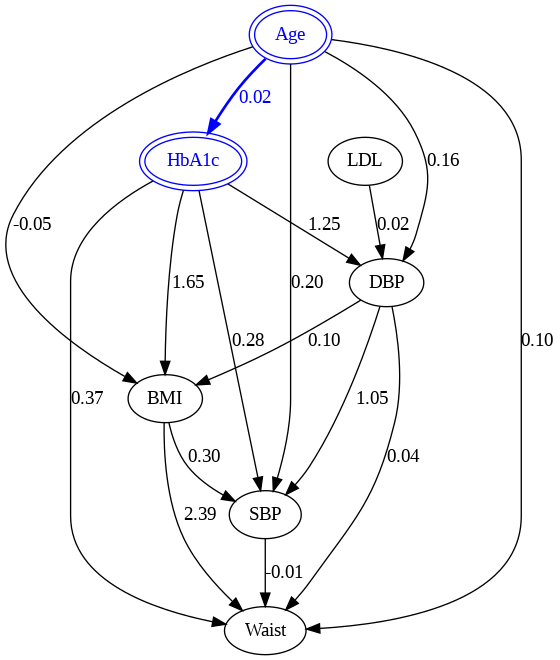
Figure 9: Causal graph suggested by DirectLiNGAM using full points of the health screening data.

For the experiment, to confirm that GPT-4 can supply SCD with adequate prior knowledge, even if a direct edge of the ground truth is not apparent, we have repeated the sampling of $1000$ points from the entire dataset, until we obtained a subset on which PC, Exact Search, and DirectLiNGAM cannot discern the causal relationship “Age”$\rightarrow$“HbA1c” without prior knowledge.

The results of the SCD on the subset are shown in Figure 10, and this subset is adopted to confirm the effectiveness of the proposed method. It is confirmed in all SCD results that “Age” $\rightarrow$ “HbA1c” does not appear, and “Age” is directly influenced by other variables, which we interpret as an unnatural behavior from the domain knowledge.

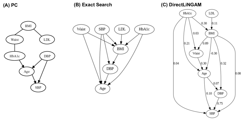
Figure 10: Results of SCD on the randomly selected subsample in the health screening dataset with (A) PC, (B) Exact Search, and (C) DirectLiNGAM.

Appendix D Composition of Adjacency Matrices Representing Causal Structure and Evaluation

D.1 Composition of Prior Knowledge Matrices

As shown in Algorithm 2, the composition rule of $PK$ depends on the type of SCD method adopted, and the decision criteria of forced and forbidden edges are tentatively set at $0.95$ and $0.05$, respectively. While PC and DirectLiNGAM can be augmented with constraints for both forced and forbidden directed edges or paths, Exact Search can only be augmented with the constraints for forbidden directed edges. In this section, the composition rule for $PK$ is described in detail for all the SCD algorithms we have adopted in this work.

For PC

As for the matrix representation of $PK$, the values of the matrix elements are determined as follows:

• Case 1. If $x_{i}\rightarrow x_{j}$ is forced (i.e., $p_{ij}\geq 0.95$), then ${\mbox{$PK$}}_{ij}$ is set to $1$.

• Case 2. If $x_{i}\rightarrow x_{j}$ is forbidden (i.e., $p_{ij}<0.05$), then ${\mbox{$PK$}}_{ij}$ is set to $0$.

• Case 3. If the existence of $x_{i}\rightarrow x_{j}$ cannot be determined immediately from the domain knowledge generated by GPT-4 (i.e., $0.05\leq p_{ij}<0.95$), then ${\mbox{$PK$}}_{ij}$ is set to $-1$.

This ternary matrix composition is based on the constraints of the prior knowledge matrix DirectLiNGAM, which will be explained later, in order to apply the generated $PK$ to DirectLiNGAM as quickly as possible. Although prior knowledge is represented as a matrix in PC algorithm widely open in “causal-learn”, both forced and forbidden edges can be set and the possibility of other unknown edges are explored. This similar properties with DirectLiNGAM means that the prior knowledge for this PC algorithm can be represented in ternary matrix, if we need to do. Therefore, the composition rule of $PK$ for PC is set to be same as that for DirectLiNGAM in this work, in order to treat it consistently as possible.

For DirectLiNGAM

Although the criteria of setting the values in $PK$ are same as those for PC, the definition of the value becomes slightly different. While the prior knowledge for PC algorithm in “causal-learn” package corresponds to the existence of directed edges between pairs of variables, the prior knowledge for DirectLiNGAM is determined with the knowledge on directed paths. The values of the matrix elements are determined as below:

• Case 1. If the directed path from $x_{i}$ to $x_{j}$ is forced (i.e., $p_{ij}\geq 0.95$), then ${\mbox{$PK$}}_{ij}$ is set to $1$.

• Case 2. If the directed path from $x_{i}$ to $x_{j}$ is forbidden (i.e., $p_{ij}<0.05$), then ${\mbox{$PK$}}_{ij}$ is set to $0$.

• Case 3. If the existence of the directed path from $x_{i}$ to $x_{j}$ cannot be determined immediately from the domain knowledge generated by GPT-4 (i.e., $0.05\leq p_{ij}<0.95$), then ${\mbox{$PK$}}_{ij}$ is set to $-1$.

This ternary matrix composition, using $1$, $0$ and $-1$ is indeed implemented in the the software package “LiNGAM”.

For Exact Search

While $PK$ in cases of PC and DirectLiNGAM is a ternary matrix, On e must be careful that $PK$ in Exact Search is a binary matrix. The values of the matrix elements are determined as below:

• Case 4. If $x_{i}\rightarrow x_{j}$ is forbidden (i.e., $p_{ij}<0.05$), then ${\mbox{$PK$}}_{ij}$ is set to $0$.

• Case 5. If $x_{i}\rightarrow x_{j}$ is forced, or the existence of this causal relationship cannot be determined immediately from the domain knowledge generated by GPT-4 (i.e., $0.05\leq p_{ij}$), then ${\mbox{$PK$}}_{ij}$ is set to $1$.

It must be carefully noted that, although the definition of ${\mbox{$PK$}}_{ij}=0$ in Case 4 for Exact Search exactly the same as that in Case 2 for PC and DirectLiNGAM, the definition of ${\mbox{$PK$}}_{ij}=1$ in Case 5 for Exact Search encompasses the both Case 1 and Case 3 for PC and DirectLiNGAM. This difference must be taken into account when evaluating $PK$ in comparison with the ground truths, in order to interpret the results in a unified manner regardless of the SCD methods used.

D.2 Composition of Ground Truth Matrix

The representation of ground truths in matrix form can be simply realized using a binary matrix, provided that it is determined whether a directed edge exists for every possible pair of variables in the system. The composition rule for the ground truth matrix $GT$ is as follows:

• If $x_{j}\rightarrow x_{j}$ exists, then ${\mbox{$GT$}}_{ij}$ is set to $1$.

• If $x_{j}\rightarrow x_{j}$ does not exist, then ${\mbox{$GT$}}_{ij}$ is set to $0$.

The matrix representations of the ground truth of the benchmark datasets of Auto MPG, DWD, and Sachs shown in Appendix C are expressed as follows:

$${\mbox{\boldmath$GT$}}_{\text{AutoMPG}}=\begin{pmatrix}0&0&0&1&0\\ 0&0&1&1&0\\ 1&0&0&0&0\\ 0&0&0&0&0\\ 0&0&1&0&0\end{pmatrix}$$ (2)

$${\mbox{\boldmath$GT$}}_{\text{DWD}}=\begin{pmatrix}0&0&0&0&0&0\\ 1&0&0&1&0&1\\ 1&0&0&1&0&0\\ 0&0&0&0&0&0\\ 1&0&0&0&0&0\\ 0&0&0&0&0&0\end{pmatrix}$$ (3)

$${\mbox{\boldmath$GT$}}_{\text{Sachs}}=\setcounter{MaxMatrixCols}{11}\begin{pmatrix}0&0&0&0&0&0&0&0&1&0&0\\ 1&0&0&0&0&0&0&1&1&0&0\\ 0&0&0&0&1&0&0&0&0&0&0\\ 0&0&1&0&1&0&0&0&0&0&0\\ 0&0&0&0&0&0&0&0&0&0&0\\ 0&1&0&0&0&0&0&1&0&0&0\\ 0&0&0&0&1&1&0&1&0&0&0\\ 0&0&0&0&0&0&0&0&1&0&0\\ 0&0&1&1&0&0&0&0&0&0&0\\ 0&0&0&0&0&0&0&1&1&0&0\\ 0&0&0&0&0&0&0&1&1&0&0\end{pmatrix}$$ (4)

D.3 Calculation of Metrics for Evaluation of Structural Consistency with Ground Truths (SHD, FPR, FNR, Precision, F1 Score)

Structural metrics such as SHD, FPR, FNR, precision and F1 score are commonly calculated for performance evaluation in various machine learning and classification contexts, and are compared with the ground truth data. In a similar context, the causal structures inferred by LLM-KBCI and SCD, especially for the benchmark datasets with known ground truths, can also be evaluated using these metrics.

For the practical evaluation of the SCD results in this study, we use the ground truth matrices defined for the benchmark datasets in Eq.(2), (3) and (4) as references, and we measure these metrics using the adjacency matrices that are calculated directly in SCD algorithms or easily transformed from the output causal graphs. Similarly, the calculation of these metrics for the evaluating LLM-KBCI outputs is carried out using $PK$.

However, it must be noted that there can be some arguments on the definition of metrics for $PK$ based on $GT$, since the definition of the matrix elements of $PK$ shown in Appendix D.1 is partially different from that of $GT$ described in Appendix D.2. In particular, while $GT_{ij}$ is a binary variable completely determined with whether $x_{j}\rightarrow x_{i}$ exists or not, ${\mbox{$PK$}}_{ij}$ can be set to $-1$ for PC and DirectLiNGAM and to $1$ for Exact Search. This indicates or includes the case where it is not impossible to definitively assert the presence or absence of $x_{j}\rightarrow x_{i}$.

Therefore, although there may be a discussion that a reasonable extension of the definitions of these metrics is required for the case above, in this study, we evaluate these metrics from $|{\mbox{\boldmath$PK$}}|$, in which both ${\mbox{$PK$}}_{ij}=1$ and ${\mbox{$PK$}}_{ij}=-1$ are interpreted as a “tentative assertion of the presence of $x_{j}\rightarrow x_{i}$” and are treated identically. This processing of $PK$ can also be interpreted as that as temporarily adopting the composition rule of $PK$ for Exact Search as is for the evaluation of SHD, FPR, FNR, precision, and F1 score, for all SCD methods. With this processing, $PK$ is handled in unified manner regardless of the SCD methods used. We believe this approach is the best way to maintain the original concept of composing $PK$, while aiming for consistent discussion across all SCD methods.

Calculation of SHD

According to the original concept of the structural hamming distance (SHD), this metric is represented as the total number of edge additions, deletions, or reversals that are needed to convert the estimated graph $G^{\prime}$ into its ground truth graph $G$ (Zheng et al., 2018; Cheng et al., 2022; Hasan et al., 2023). As in our study, if network graphs $G$ and $G^{\prime}$ are represented by binary matrices $\bm{G}$ and $\bm{G^{\prime}}$, respectively, where all elements are either $0$ or $1$, then the total number of edge additions ($A$), deletions ($D$), and reversals ($R$) can be simply calculated as follows:

$$A(\bm{G^{\prime}},\bm{G}) =\sum_{i,j}\bm{1}(G_{ij})\bm{1}(G_{ji})\bm{1}(G_{ij}^{\prime}-1)$$ (5)

$$\rule{0.0pt}{14.22636pt}D(\bm{G^{\prime}},\bm{G}) =\sum_{i,j}\bm{1}(G_{ij}^{\prime})\bm{1}(G_{ji}^{\prime})\bm{1}(G_{ij}-1)$$ (6)

$$\rule{0.0pt}{14.22636pt}R(\bm{G^{\prime}},\bm{G}) =\sum_{i,j}\bm{1}(G_{ij})\bm{1}(G_{ji}-1)\bm{1}(G_{ij}^{\prime}-1)\bm{1}(G_{ji}^{\prime})$$ (7)

Here, we introduce the indicator function $\bm{1}(x)$, expressed as:

$$\bm{1}(x)=\begin{cases}1&\text{if }x=0,\\ 0&\text{otherwise }(x\neq 0).\end{cases}$$ (8)

Since SHD is defined as $\text{{SHD}}=A+D+R$, it is easily evaluated as:

$$\text{{SHD}}(\bm{G^{\prime}},\bm{G})=\\ \sum_{i,j}\Bigl{\{}~{}~{}\bm{1}(G_{ij})\bm{1}(G_{ji})\bm{1}(G_{ij}^{\prime}-1)~{}+~{}\bm{1}(G_{ij}^{\prime})\bm{1}(G_{ji}^{\prime})\bm{1}(G_{ij}-1)~{}+~{}\bm{1}(G_{ij})\bm{1}(G_{ji}-1)\bm{1}(G_{ij}^{\prime}-1)\bm{1}(G_{ji}^{\prime})~{}~{}\Bigr{\}}$$ (9)

For the evaluation of SHD of LLM-KBCI outputs, $\text{{SHD}}(|{\mbox{\boldmath$PK$}}|,{\mbox{\boldmath$GT$}})$ is calculated with Eq. (9).

Calculation of FPR, FNR, Precision and F1score

In the similar context to SHD, for calculation of the metrics such as false positive rate (FPR) and false negative rate (FNR), we prepare the equation for evaluating the number of true positive (TP), false positive (FP), true negative (TN), and false negative (FN) edges as follows:

$$\text{{TP}}(\bm{G^{\prime}},\bm{G}) =\sum_{i,j}\bm{1}(G_{ij}-1)\bm{1}(G_{ij}^{\prime}-1)$$ (10)

$$\rule{0.0pt}{14.22636pt}\text{{FP}}(\bm{G^{\prime}},\bm{G}) =\sum_{i,j}\bm{1}(G_{ij})\bm{1}(G_{ij}^{\prime}-1)$$ (11)

$$\rule{0.0pt}{14.22636pt}\text{{TN}}(\bm{G^{\prime}},\bm{G}) =\sum_{i,j}\bm{1}(G_{ij})\bm{1}(G_{ij}^{\prime})$$ (12)

$$\rule{0.0pt}{14.22636pt}\text{{FN}}(\bm{G^{\prime}},\bm{G}) =\sum_{i,j}\bm{1}(G_{ij}-1)\bm{1}(G_{ij}^{\prime})$$ (13)

Then, using Eq. (10)– (13), the definition of FPR, FNR, precision, and F1 score can be expressed as follows:

$$\text{{FPR}}(\bm{G^{\prime}},\bm{G}) =\frac{\text{{FP}}(\bm{G^{\prime}},\bm{G})}{\text{{TN}}(\bm{G^{\prime}},\bm{G})+\text{{FP}}(\bm{G^{\prime}},\bm{G})}$$ (14)

$$\rule{0.0pt}{22.76219pt}\text{{FNR}}(\bm{G^{\prime}},\bm{G}) =\frac{\text{{FN}}(\bm{G^{\prime}},\bm{G})}{\text{{TP}}(\bm{G^{\prime}},\bm{G})+\text{{FN}}(\bm{G^{\prime}},\bm{G})}$$ (15)

$$\rule{0.0pt}{22.76219pt}\text{{Precision}}(\bm{G^{\prime}},\bm{G}) =\frac{\text{{TP}}(\bm{G^{\prime}},\bm{G})}{\text{{TP}}(\bm{G^{\prime}},\bm{G})+\text{{FP}}(\bm{G^{\prime}},\bm{G})}$$ (16)

$$\rule{0.0pt}{22.76219pt}\text{{F${}_{1}$score}}(\bm{G^{\prime}},\bm{G}) =\frac{2\,\text{{TP}}(\bm{G^{\prime}},\bm{G})}{2\,\text{{TP}}(\bm{G^{\prime}},\bm{G})+\text{{FN}}(\bm{G^{\prime}},\bm{G})+\text{{FP}}(\bm{G^{\prime}},\bm{G})}$$ (17)

For the evaluation of structural metrics such as FPR of LLM-KBCI outputs, $\text{{FPR}}(|{\mbox{\boldmath$PK$}}|,{\mbox{\boldmath$GT$}})$, $\text{{FNR}}(|{\mbox{\boldmath$PK$}}|,{\mbox{\boldmath$GT$}})$, $\text{{Precision}}(|{\mbox{\boldmath$PK$}}|,{\mbox{\boldmath$GT$}})$ and $\text{{F${}_{1}$score}}(|{\mbox{\boldmath$PK$}}|,{\mbox{\boldmath$GT$}})$ are calculated with Eq. (14)–(17).

Appendix E Algorithm $A$ for Transformation of Cyclic $PK$ into Acyclic Adjacency Matrices and Selection of the Optimal Matrix

As briefly described in Section 3.1, for the case of DirectLiNGAM, acyclicity of $PK$ is also required. Thus, if the $PK$ directly calculated from the probability matrix is cyclic, it must be transformed into an acyclic form. One possible method is to delete the minimum number of edges included in cycles to transform $PK$ into an acyclic matrix. However, it is possible that there are several solutions transformed from the same $PK$ with the minimum manipulation of deleting edges. Therefore, we have decided to carry out causal discovery with DirectLiNGAM for every possible acyclic prior knowledge matrix to select the best acyclic prior knowledge matrix ${\mbox{\boldmath$PK$}}_{A}$ in terms of statistical modeling. The dataset is again fitted with a structural equation model under the constraint of the causal structure explored with DirectLiNGAM, assuming linear-Gaussian data, and the Bayes Information Criterion (BIC) is calculated. After repeating this process, the acyclic prior knowledge matrix with which the BIC becomes the lowest is selected as ${\mbox{\boldmath$PK$}}_{A}$.

The overall transformation process is described in Algorithm 3. However, in the practical application of this method, it must be noted that completing the list of acyclic prior knowledge matrices $A$ incurs significant computational costs. Hence, as the number of variables increases, completing this calculation algorithm in a realistic time frame becomes more challenging.

For the future generalization and application of our inference method using DirectLiNGAM, the development of more efficient algorithms for transforming a cyclic matrix into an acyclic one is anticipated.

Algorithm 3 Transformation of Cyclic $PK$ into Acyclic Adjacency Matrices and Selection of the Optimal Matrix

  Input 1: Cyclic prior knowledge matrix ${\mbox{\boldmath$PK$}}\bm{{}_{C}}$

  Input 2: Data $X$ with variables$\{x_{1},...,x_{n}\}$

  Input 3: DirectLiNGAM Algorithm $L(X,{\mbox{\boldmath$PK$}})$

  Output: Optimal acyclic matrix ${\mbox{\boldmath$PK$}}\bm{{}_{A}}$

  Initialize the temporal set for matrices $\bm{T}\leftarrow\{{\mbox{\boldmath$PK$}}\bm{{}_{C}}\}$

  Initialize the temporal set for number of the cycles $\bm{N}\leftarrow\{\}$

  Initialize the temporal set for acyclic matrices $\bm{A}\leftarrow\{\}$

  repeat

     for matrix $\bm{T}_{m}\in\bm{T}$ do

        Count the number of cycles in $\bm{T}_{m}$ as $N_{m}$

        Add $N_{m}$ to $\bm{N}$

     end for

     if $\exists\bm{N}_{m}\in\bm{N}$ $N_{m}=0$ then

        Detect all $\bm{T}_{m}$, which satisfies $N_{m}=0$ and add them to $\bm{A}$

     else

        Initialize the temporal set for modified matrices $\bm{T}^{\prime}\leftarrow\{\}$

        for $\bm{T}_{m}\in\bm{T}$ do

           Initialize the set for edges included in cycles $\bm{E}_{m}\leftarrow\{\}$

           Initialize the set for edges to be removed $\bm{F}_{m}\leftarrow\{\}$

           Detect all cycles in $\bm{T}_{m}$

           For each detected cycle, identify all the edges that form the cycle

           Add these edges to a set of edges to be removed $\bm{E}_{m}$

           Detect the most frequent edges “$x_{i}\leftarrow x_{j}$” in $\bm{E}_{m}$ as $(i,j)_{f}$

           $\forall(i_{f},j_{f})$ add $(i_{f},j_{f})$ to $\bm{F}_{m}$

           for $(i_{f},j_{f})\in\bm{F}_{m}$ do

              $\bm{T^{\prime}}_{m}=\bm{T}_{m}$

              $\bm{T^{\prime}}_{m}(i_{f},j_{f})\leftarrow 0$

              Add ${\bm{T^{\prime}}_{m}}$ to $\bm{T}^{\prime}$

           end for

        end for

        Replace $\bm{T}$ with $\bm{T}^{\prime}$

     end if

  until $\bm{A}$ is not empty

  Initialize the optimal BIC value $B=\text{None}$

  Initialize the optimal acyclic matrix for prior knowledge in DirectLiNGAM $\bm{A}_{\text{optimal BIC}}=\text{None}$

  for $\bm{A}_{m}\in\bm{A}$ do

     Calculate adjacency matrix (with the components 0 or 1) of the causal discovery result ${\mbox{\boldmath$Adj$}}=L(X,{\mbox{\boldmath$PK$}}=\bm{A}_{m})$

     Fit $X$ with the structural causal equation model represented in $Adj$ assuming linear-Gaussian data

     Calculate BIC with $Adj$ and $X$ as $B_{\text{temp}}$

     if $B>B_{\text{temp}}$ or $B={\text{None}}$ then

        $B\leftarrow B_{\text{temp}}$

        $\bm{A}_{\text{optimal BIC}}=\bm{A_{m}}$

     end if

  end for

  return $\bm{A}_{\text{optimal BIC}}$ as ${\mbox{\boldmath$PK$}}\bm{{}_{A}}$

Appendix F Details of LLM-KBCI Results

It is also valuable to examine the details of the probability matrices generated by LLM-KBCI, both for the basic discussion on whether LLMs can generate a valid interpretation of causality from a domain expert’s point of view, and for understanding the characteristics of SCP. In this section, the probability matrices generated by GPT-4 for Auto MPG data and DWD climate data, which are relatively easy to interpret within common daily knowledge, are shown and briefly interpreted. For comparison among various SCP patterns (Patterns 1–4) using the same SCD method as much as possible, the probability matrices generated by GPT-4 with SCP are shown only for DirectLiNGAM. We also briefly present the probability matrices of LLM-KBCI for the sampled sub-dataset of health screening results.

F.1 LLM-KBCI for Auto MPG data

In Table 11, the probabilities of causal relationships of pairs of variables in Auto MPG data are shown. The cells highlighted in green are the ones in which the directed edges are expected to appear from the ground truths shown in Figure 3.

For all the prompting patterns, While the probability of “Weight”$\rightarrow$“Displacement”, which is interpreted as one of the ground truth directed edges, is $0$, the probability of reversed edge “Displacement”$\rightarrow$“Weight” is non-zero and over $0.95$ in Patterns 1–4. For understanding this behavior and elucidating the true causal relationship between these two variables, further discussion is required, including the possibility of the hidden common causes which are excluded from the dataset we have used.

In addition to that, although we do not believe the existence of the directed edge of “Displacement”$\rightarrow$“Acceleration”, the probability of this causal relationship is over $0.85$ for all the prompting patterns. This may be due to the property of the prompting for evaluating the probability. As shown in Table 2, GPT-4 is allowed to judge the existence of both direct and indirect causal relationships, in order to acquire positive answer even if any intervening variables are not included in the dataset. However, for example, considering that the probabilities of both “Displacement”$\rightarrow$“Horsepower” and “Horsepower”$\rightarrow$“Acceleration”, which are part of the ground truths, are relatively high, it is also possible that GPT-4 support the hypothesis of some impact from “Displacement” on “Acceleration” partially due to the confidence in the indirect causal relationship of “Displacement”$\rightarrow$“Horsepower”$\rightarrow$“Acceleration”. If one wants to distinguish the direct and indirect causal relationships in the interpretation of the probability matrix, investigation of the response from LLMs for the first prompting may lead to further understanding.

Some differences which can be related to the prompting patterns can be also observed. For example, the probability of “Horsepower”$\rightarrow$“Mpg” in Pattern 1 is much smaller than other patterns. Moreover, the probabilities of “Horsepower”$\rightarrow$“Acceleration” in Pattern 1 and 3 are smaller than other patterns, in which the probability of this edge is almost $1$. A possible explanation of these behaviors is that the decision-making of GPT-4 is unsettled with SCP, in which the causal structure inferred by DirectLiNGAM shown in Figure 4 (c) is included. Since neither “Horsepower”$\rightarrow$“Acceleration” nor “Horsepower”$\rightarrow$“Mpg” appears in Figure 4 (c), despite the confidence in the existence of these edges only from the domain knowledge, the decision-making of GPT-4 may become more careful, taking into account the result of SCD. It is desired to elucidate what kinds of decision-making of LLMs are likely to be affected by SCP in the future works.

Table 11: Probabilities of the causal relationships suggested by GPT-4 in Auto MPG data. The cells in which the directed edges are expected to appear from the ground truths as shown in Figure 3 are highlighted in green.

Pattern 0 EFFECTED\CAUSE “Displacement” “Mpg” “Horsepower” “Weight” “Aceleration” “Displacement” - 0.000 0.000 0.000 0.000 “Mpg” 0.999 - 0.997 1.000 1.000 “Horsepower” 0.999 0.000 - 0.000 0.000 “Weight” 0.635 0.000 0.000 - 0.000 “Aceleration” 0.996 0.023 0.998 0.998 - Pattern 1 EFFECTED\CAUSE “Displacement” “Mpg” “Horsepower” “Weight” “Aceleration” “Displacement” - 0.000 0.000 0.000 0.000 “Mpg” 1.000 - 0.128 0.484 0.058 “Horsepower” 1.000 0.056 - 0.001 0.000 “Weight” 0.994 0.000 0.000 - 0.000 “Aceleration” 0.859 0.000 0.828 0.998 - Pattern 2 EFFECTED\CAUSE “Displacement” “Mpg” “Horsepower” “Weight” “Aceleration” “Displacement” - 0.000 0.000 0.000 0.000 “Mpg” 1.000 - 0.999 1.000 0.984 “Horsepower” 1.000 0.000 - 0.000 0.000 “Weight” 0.997 0.000 0.000 - 0.000 “Aceleration” 0.995 0.002 0.996 0.999 - Pattern 3 EFFECTED\CAUSE “Displacement” “Mpg” “Horsepower” “Weight” “Aceleration” “Displacement” - 0.000 0.000 0.000 0.000 “Mpg” 0.977 - 0.969 0.754 0.547 “Horsepower” 1.000 0.051 - 0.696 0.010 “Weight” 0.954 0.000 0.000 - 0.000 “Aceleration” 0.981 0.000 0.435 0.809 - Pattern 4 EFFECTED\CAUSE “Displacement” “Mpg” “Horsepower” “Weight” “Aceleration” “Displacement” - 0.000 0.000 0.000 0.000 “Mpg” 0.995 - 0.994 0.997 0.940 “Horsepower” 0.999 0.314 - 0.006 0.000 “Weight” 0.999 0.000 0.012 - 0.000 “Aceleration” 0.964 0.000 0.989 0.814 -

F.2 LLM-KBCI for DWD climate data

In Table 12, the probabilities of the causal relationships of pairs of variables in DWD climate data are shown. The cells highlighted in green are the ones in which the directed edges are expected to appear from the ground truths shown in Figure 5.

For all the prompting patterns, it is confirmed that all of the probabilities of the causal effects on “Altitude”,“Longitude” and “Latitude” from other variables are $0$. Since these three variables are geographically given and fixed, the interpretation by GPT-4 that they act as parent variables that are not influenced by other factors is completely reasonable. Although “Altitude” and “Latitude” are somehow influenced according to the result of DirectLiNGAM without prior knowledge as shown in Figure 6 (c), SCP including these unnatural results has not affected on the decision-making by GPT-4. From this behavior, it is inferred that the response regarding axiomatic and self-evident matters from GPT-4 is robust and not likely to be affected by SCP, even if the SCD result exhibits obviously unnatural behaviors.

In addition, while “Longitude”$\rightarrow$“Temperature”, which are assumed to be a ground truth, is not likely to be asserted by GPT-4, “Temperature”$\rightarrow$“Precipitation”, which is not expected to be a ground truth, is likely to be asserted by GPT-4, across all the prompting patterns. For further interpretation of these unexpected behaviors from our ground truths, investigation of the response generated in the first prompting process is recommended. It is also interesting that while the probabilities of “Longitude”$\rightarrow$“Precititation” are $0$ in Patterns 0–2, they become non-zero finite values in Patterns 3 and 4, in which the causal coefficient of this directed edge calculated with DirectLiNGAM is included in SCP. This behavior may be a glimpse that SCP can assist the decision-making of GPT-4 even if it generates an incomplete response on causal relationships with its background knowledge.

Table 12: Probabilities of the causal relationships suggested by GPT-4 in DWD climate data. The cells in which the directed edges are expected to appear from the ground truths as shown in Figure 5 are highlighted in green.

Pattern 0 EFFECTED\CAUSE “Altitude” “Temperature” “Precipitation” “Longitude” “Sunshine” “Latitude” “Altitude” - 0.000 0.000 0.000 0.000 0.000 “Temperture” 1.000 - 0.891 0.000 1.000 1.000 “Precipitation” 1.000 0.999 - 0.000 0.001 0.995 “Longitude” 0.000 0.000 0.000 - 0.000 0.000 “Sunshine” 1.000 0.000 0.998 0.000 - 1.000 “Latitude” 0.000 0.000 0.000 0.000 0.000 - Pattern 1 EFFECTED\CAUSE “Altitude” “Temperature” “Precipitation” “Longitude” “Sunshine” “Latitude” “Altitude” - 0.000 0.000 0.000 0.000 0.000 “Temperture” 0.384 - 0.034 0.000 0.856 0.011 “Precipitation” 0.025 0.999 - 0.000 0.036 0.026 “Longitude” 0.000 0.000 0.000 - 0.000 0.000 “Sunshine” 0.006 0.011 0.008 0.000 - 0.596 “Latitude” 0.000 0.000 0.000 0.000 0.000 - Pattern 2 EFFECTED\CAUSE “Altitude” “Temperature” “Precipitation” “Longitude” “Sunshine” “Latitude” “Altitude” - 0.000 0.000 0.000 0.000 0.000 “Temperture” 0.997 - 0.007 0.000 0.999 0.989 “Precipitation” 0.739 0.999 - 0.000 0.000 0.384 “Longitude” 0.000 0.000 0.000 - 0.000 0.000 “Sunshine” 0.874 0.010 0.976 0.000 - 0.981 “Latitude” 0.000 0.000 0.000 0.000 0.000 - Pattern 3 EFFECTED\CAUSE “Altitude” “Temperature” “Precipitation” “Longitude” “Sunshine” “Latitude” “Altitude” - 0.000 0.000 0.000 0.000 0.000 “Temperture” 0.919 - 0.016 0.003 0.615 0.973 “Precipitation” 0.585 0.996 - 0.175 0.002 0.008 “Longitude” 0.000 0.000 0.000 - 0.000 0.000 “Sunshine” 0.039 0.000 0.001 0.875 - 0.199 “Latitude” 0.000 0.000 0.000 0.000 0.000 - Pattern 4 EFFECTED\CAUSE “Altitude” “Temperature” “Precipitation” “Longitude” “Sunshine” “Latitude” “Altitude” - 0.000 0.000 0.000 0.000 0.000 “Temperture” 0.982 - 0.023 0.029 0.990 0.958 “Precipitation” 0.826 0.987 - 0.927 0.010 0.797 “Longitude” 0.000 0.000 0.000 - 0.000 0.000 “Sunshine” 0.534 0.021 0.387 0.013 - 0.638 “Latitude” 0.000 0.000 0.000 0.000 0.000 -

F.3 LLM-KBCI for Dataset of Health Screening Results

In Table 13, the probabilities of the causal relationships of pairs of variables in our sampled sub-dataset of health screening results are shown. The cells highlighted in red are the ones in which the directed edges are expected to appear as described in Appendix C.4. In contrast, since “Age” is an unmodifiable background factor, it can be concluded that it is not a descendant of any other variables. Therefore, the probabilities in the cells highlighted in blue are expected to be $0$.

Across all the prompting patterns, it is confirmed that all of probabilities of the causal effects on “Age” from other variables are indeed $0$. From this fact, it is likely to be regarded by GPT-4 as axiomatic and self-evident that “Age” cannot be affected from other variables, and the judge of the causal relationships is not influenced by SCP, even if the SCD result exhibits obviously unnatural behaviors as shown in Figure 10.

Table 13: Probabilities of the causal relationships suggested by GPT-4 in the sampled sub-dataset of health screening results. The cells in which the directed edges are expected to appear from the ground truths are highlighted in red. In contrast, the probabilities in the cells highlighted in blue, are expected to be zero, since “Age” is expected to be a parent variable for all other variables.

Pattern 0 EFFECTED\CAUSE “BMI” “Waist” “SBP” “DBP” “HbA1c” “LDL” “Age” “BMI” - 0.994 0.000 0.000 0.000 0.000 0.901 “Waist” 1.000 - 0.000 0.000 0.000 0.000 0.353 “SBP” 0.999 0.962 - 0.998 0.987 0.000 0.626 “DBP” 0.998 0.995 0.993 - 0.000 0.000 0.001 “HbA1c” 0.998 0.998 0.000 0.000 - 0.000 0.986 “LDL” 0.988 0.967 0.000 0.000 0.000 - 0.002 “Age” 0.000 0.000 0.000 0.000 0.000 0.000 - Pattern 1 EFFECTED\CAUSE “BMI” “Waist” “SBP” “DBP” “HbA1c” “LDL” “Age” “BMI” - 0.312 0.000 0.000 0.014 0.000 0.076 “Waist” 1.000 - 0.000 0.000 0.023 0.000 0.043 “SBP” 0.999 0.912 - 0.999 0.997 0.000 0.302 “DBP” 0.998 0.421 0.050 - 0.000 0.000 0.019 “HbA1c” 0.517 0.503 0.101 0.000 - 0.000 0.170 “LDL” 0.008 0.527 0.000 0.000 0.000 - 0.517 “Age” 0.000 0.000 0.000 0.000 0.000 0.000 - Pattern 2 EFFECTED\CAUSE “BMI” “Waist” “SBP” “DBP” “HbA1c” “LDL” “Age” “BMI” - 0.998 0.001 0.001 0.996 0.000 0.093 “Waist” 0.999 - 0.000 0.003 0.959 0.007 0.099 “SBP” 0.998 0.994 - 0.983 0.994 0.040 0.207 “DBP” 0.997 0.975 0.984 - 0.983 0.002 0.115 “HbA1c” 0.982 0.608 0.002 0.000 - 0.000 0.723 “LDL” 0.994 0.946 0.000 0.000 0.452 - 0.171 “Age” 0.000 0.000 0.000 0.000 0.000 0.000 - Pattern 3 EFFECTED\CAUSE “BMI” “Waist” “SBP” “DBP” “HbA1c” “LDL” “Age” “BMI” - 0.003 0.000 0.000 0.868 0.923 0.306 “Waist” 1.000 - 0.000 0.000 0.983 0.000 0.076 “SBP” 1.000 0.855 - 0.959 0.999 0.000 0.235 “DBP” 1.000 0.032 0.140 - 0.021 0.000 0.095 “HbA1c” 0.967 0.634 0.000 0.000 - 0.000 0.046 “LDL” 0.562 0.165 0.000 0.000 0.085 - 0.013 “Age” 0.000 0.000 0.000 0.000 0.000 0.000 - Pattern 4 EFFECTED\CAUSE “BMI” “Waist” “SBP” “DBP” “HbA1c” “LDL” “Age” “BMI” - 0.993 0.000 0.000 0.024 0.006 0.037 “Waist” 1.000 - 0.000 0.000 0.957 0.000 0.395 “SBP” 0.999 0.982 - 0.001 0.998 0.000 0.795 “DBP” 0.994 0.204 0.985 - 0.408 0.000 0.926 “HbA1c” 0.824 0.391 0.000 0.000 - 0.000 0.176 “LDL” 0.485 0.403 0.000 0.000 0.000 - 0.027 “Age” 0.000 0.000 0.000 0.000 0.000 0.000 -

Appendix G Details of SCD with Prior Knowledge Augmentation from GPT-4 in All benchmark Datasets

In Table 14, the details of SCD results augmented with $PK$ generated from GPT-4 are shown for all the benchmark datasets, which are introduced in Appendix C. As shown in section 4, the results on DWD climate data have been already introduced and discussed, and it has been confirmed that our method of integrating SCD and LLM-KBCI, including SCP, indeed contributes to the enhancement of precision and statistical validity of the causal models. Although an overview of the results for the Auto MPG and Sachs datasets are almost same as that for the DWD dataset, confirming and comparison of the behaviors of all benchmark datasets can be valuable, both for confirming the universality of the benefits brought about with our method, and for deeper understanding of the benefits.

Table 14: Comparison of the SCD results (and structural familiarity of $PK$ with ground truths, for evaluation of the performance of LLM-KBCI) in all the experiment patterns we have conducted. Lower values are superior for SHD, FPR, FNR, RMSEA and BIC, and higher values for precision, F1score and CFI. It is implied that in DWD and Sachs datasets, the outputs of LLM-KBCI in Patterns 1–4 are likely to approach the ground truths more closely than those in Pattern 0. It is also suggested that several of the outputs of Exact Search and DirectLiNGAM in Pattern 1–4 (with SCP), can be superior causal models than those in Pattern 0.

SCD algorithm	Pattern	SHD	FPR	FNR	Precision	F1score	CFI	RMSEA	BIC
1. Auto MPG data with 5 continuous variables
PC	wo $PK$	8	0.40	0.80	0.11	0.14	1.00	0.00	71.65
	Pattern 0	3 (5)	0.15 (0.25)	0.20 (0.20)	0.57 (0.44)	0.67 (0.57)	1.00	0.07	65.62
	Pattern 1	4 (7)	0.15 (0.30)	0.20 (0.20)	0.57 (0.40)	0.67 (0.53)	1.00	0.00	59.71
	Pattern 2	3 (6)	0.15 (0.30)	0.20 (0.20)	0.57 (0.40)	0.67 (0.53)	1.00	0.07	65.62
Exact Search	wo $PK$	5	0.25	0.40	0.38	0.46	1.00	0.07	71.61
	Pattern 0	4 (5)	0.20 (0.25)	0.20 (0.20)	0.50 (0.44)	0.62 (0.57)	1.00	0.09	71.59
	Pattern 1	5 (5)	0.20 (0.20)	0.20 (0.20)	0.50 (0.50)	0.62 (0.62)	1.00	0.07	65.62
	Pattern 2	4 (5)	0.20 (0.25)	0.20 (0.20)	0.50 (0.44)	0.62 (0.57)	1.00	0.09	71.59
DirectLiNGAM	wo $PK$	8	0.40	0.80	0.11	0.14	1.00	0.05	77.61
	Pattern 0	3 (5)	0.15 (0.25)	0.20 (0.20)	0.57 (0.44)	0.67 (0.57)	1.00	0.07	65.62
	Pattern 1	3 (5)	0.15 (0.30)	0.20 (0.20)	0.57 (0.40)	0.67 (0.53)	1.00	0.07	65.62
	Pattern 2	3 (5)	0.15 (0.25)	0.20 (0.20)	0.57 (0.44)	0.67 (0.57)	1.00	0.07	65.62
	Pattern 3	4 (6)	0.20 (0.35)	0.20 (0.20)	0.50 (0.36)	0.62 (0.50)	1.00	0.00	71.65
	Pattern 4	3 (5)	0.15 (0.30)	0.20 (0.20)	0.57 (0.40)	0.67 (0.53)	1.00	0.07	65.62
2. DWD climate data with 6 continuous variables
PC	wo $PK$	9	0.20	0.83	0.14	0.15	0.90	0.22	69.32
	Pattern 0	5 (8)	0.03 (0.20)	0.67 (0.33)	0.67 (0.40)	0.44 (0.50)	0.71	0.36	32.70
	Pattern 1	5 (9)	0.03 (0.23)	0.67 (0.33)	0.67 (0.36)	0.44 (0.47)	0.71	0.36	32.70
	Pattern 2	5 (8)	0.03 (0.20)	0.67 (0.33)	0.67 (0.40)	0.44 (0.50)	0.71	0.36	32.70
Exact Search	wo $PK$	6	0.20	0.17	0.45	0.59	0.91	0.28	92.87
	Pattern 0	5 (8)	0.10 (0.20)	0.33 (0.33)	0.57 (0.40)	0.62 (0.50)	0.98	0.12	58.38
	Pattern 1	5 (5)	0.10 (0.13)	0.33 (0.17)	0.57 (0.56)	0.62 (0.67)	0.91	0.19	57.73
	Pattern 2	6 (9)	0.13 (0.23)	0.33 (0.33)	0.50 (0.36)	0.57 (0.47)	0.91	0.20	63.58
DirectLiNGAM	wo $PK$	10	0.33	0.67	0.17	0.22	1.00	0.00	99.53
	Pattern 0	4 (8)	0.07 (0.20)	0.33 (0.33)	0.67 (0.40)	0.67 (0.50)	1.00	0.00	52.67
	Pattern 1	8 (8)	0.10 (0.10)	0.83 (0.83)	0.25 (0.25)	0.20 (0.20)	0.64	0.43	38.03
	Pattern 2	4 (7)	0.03 (0.17)	0.50 (0.33)	0.75 (0.44)	0.60 (0.53)	0.98	0.09	40.80
	Pattern 3	5 (6)	0.10 (0.13)	0.33 (0.33)	0.57 (0.50)	0.62 (0.57)	0.93	0.16	57.90
	Pattern 4	5 (6)	0.10 (0.17)	0.33 (0.16)	0.57 (0.50)	0.62 (0.62)	0.92	0.18	57.80
3. Sachs’ protein data with 11 continuous variables
PC	wo $PK$	24	0.16	0.47	0.38	0.44	0.99	0.05	294.15
	Pattern 0	15 (19)	0.04 (0.11)	0.58 (0.47)	0.67 (0.48)	0.52 (0.50)	0.89	0.16	166.91
	Pattern 1	25 (43)	0.17 (0.53)	0.68 (0.16)	0.26 (0.23)	0.29 (0.36)	0.97	0.11	284.58
	Pattern 2	23 (23)	0.13 (0.24)	0.74 (0.32)	0.28 (0.35)	0.27 (0.46)	0.97	0.09	231.27
Exact Search	wo $PK$	31	0.26	0.68	0.18	0.23	0.99	0.07	374.35
	Pattern 0	17 (19)	0.07 (0.11)	0.58 (0.47)	0.53 (0.48)	0.47 (0.50)	0.91	0.16	202.97
	Pattern 1	17 (15)	0.05 (0.06)	0.68 (0.58)	0.55 (0.57)	0.40 (0.48)	0.87	0.20	158.26
	Pattern 2	16 (14)	0.11 (0.14)	0.53 (0.32)	0.45 (0.48)	0.46 (0.57)	0.95	0.12	257.53
DirectLiNGAM	wo $PK$	29	0.25	0.47	0.28	0.36	1.00	0.01	410.23
	Pattern 0	17 (19)	0.07 (0.11)	0.53 (0.47)	0.56 (0.48)	0.51 (0.50)	0.91	0.16	203.02
	Pattern 1	15 (13)	0.07 (0.08)	0.47 (0.37)	0.59 (0.60)	0.56 (0.62)	0.88	0.18	220.32
	Pattern 2	22 (21)	0.14 (0.18)	0.63 (0.47)	0.33 (0.36)	0.35 (0.43)	0.70	0.31	269.76
	Pattern 3	22 (23)	0.15 (0.18)	0.53 (0.53)	0.38 (0.33)	0.42 (0.39)	0.92	0.16	301.51
	Pattern 4	20 (16)	0.12 (0.16)	0.53 (0.26)	0.43 (0.47)	0.45 (0.57)	0.89	0.19	264.97

One of the characteristics in Table 14 is that in most of the cases, the result of SCD augmented with $PK$ is more similar to $GT$ than the first SCD result without prior knowledge. This behavior is interpreted as the knowledge-based improvement of the causal graph by GPT-4 as a domain expert, which is qualitatively consistent with other related works on LLM-guided causal inference (Ban et al., 2023; Vashishtha et al., 2023). Moreover, in many of the cases of Auto MPG and DWD data, the precision or F1 score are higher after the SCD augmented with $PK$ than the pure $PK$, which are conclusions of LLM-KBCI using GPT-4, while they are almost comparable in the cases of Sachs data. From this comparison it is implied that even if LLM-KBCI is optimal, the ground truths can be better approached, by conducting SCD augmented with LLM-KBCI. In addition, BIC decreases in almost all the patterns from the SCD result without $PK$. The aforementioned properties suggest that knowledge based augmentation from GPT-4 can improve the performance of SCD, indeed, in terms of the consistency with respect to the domain expert knowledge and statistical causal structure.

However, the amount of the improvement can be different depending on the number of variables and the methods of SCD.

Dependence on the number of variables

In the case of Auto MPG data with only 5 variables, the amount of improvement is almost constant among all the prompting patterns for each SCD method. One of the possible reasons is that within relatively small numbers of variable, the amount of information included in SCP becomes small, and the difference of inference performance of GPT-4 among the prompting patterns becomes subtle. Moreover, since the space for discovery becomes also smaller along with the network shrink, the SCD algorithm may reach a single optimal solution, even if $PK$ is different.

On the other hand, in the cases of DWD data with 6 variables and Sachs data 11 variables, the difference in the amount of the improvement becomes more clear depending on the prompting patterns. From this fact, it is implied that the threshold of the number of variables over which the quality of $PK$ and SCD results depend on the amount of information included in SCP for GPT-4, is around 5.

Moreover, in many cases of DWD and Sachs data, in particular when Exact Search or DirectLiNGAM is adopted, the precision and F1 score of $PK$ generated from Pattern 0 are usually smaller than any of other patterns, in which GPT-4 experiences SCP. This fact suggests that the performance of LLM-KBCI is indeed likely to be enhanced by SCP, although it is still unknown how the contents in SCP improves the response of GPT-4 for LLM-KBCI.

Prompting pattern dependence on SCD methods

Considering the output of the SCD augmented with $PK$, Pattern 0 stably indicates relatively higher performance among all the patterns in both terms of domain knowledge and statistical model fitting, in particular when the PC algorithm is used. Although it is difficult to explain the reason of this behavior, one of the possible reasons, if we focus only on the results on Sachs data, is that we adopted the ground truth which is partially determined by Bayesian network inference (Sachs et al., 2005). Indeed, the first SCD result in PC has been already relatively close to the ground truth, as shown in Figure 8 (a), and we interpret that in this kind of situation, the performance of SCD with the prior knowledge cannot be improved any more.

The scenario differs when we use the DirectLiNGAM algorithm. The quality of SCD output augmented with $PK$ either in Pattern 1 or 2, remains totally superior to that of Pattern 0 from both statistical and domain expert points of view. This implies that SCP can effectively improve the performance of and DirectLiNGAM.

However, from the analysis of Patterns 3 and 4, in which GPT-4 is prompted with the causal coefficients of the first SCD results, it is also revealed that prompting with a greater amount of statistical information does not always lead to improved SCD results. In particular, while $PK$ in Pattern 4 is closer to ground truth matrix than that in Pattern 0 in DWD or Sachs data , the final SCD result augmented with $PK$ in Pattern 4 is inferior to that of Pattern 0. One of the possible reasons of this may be the pruning of the candidate edges suggested from $PK$ in the SCD process. Including this problem, further researches are expected on what the kind and amount of information in SCP can really maximize the performance of SCD, for the generalization and practical application of our method.

References

- Abdullahi et al. (2020) Abdullahi, U. I., Samothrakis, S., and Fasli, M. Causal inference with correlation alignment. In Proc. 2020 IEEE International Conference on Big Data (Big Data), pp. 4971–4980, 2020. doi: 10.1109/BigData50022.2020.9378334.
- Alley et al. (2008) Alley, D. E., Ferrucci, L., Barbagallo, M., Studenski, S. A., and Harris, T. B. A Research Agenda: The Changing Relationship Between Body Weight and Health in Aging. The Journals of Gerontology: Series A, 63(11):1257–1259, 11 2008. ISSN 1079-5006. doi: 10.1093/gerona/63.11.1257. URL https://doi.org/10.1093/gerona/63.11.1257.
- Ban et al. (2023) Ban, T., Chen, L., Lyu, D., Wang, X., and Chen, H. Causal structure learning supervised by large language model. arXiv preprint, 2023. doi: 10.48550/arXiv.2311.11689.
- Bentler (1990) Bentler, P. M. Comparative fit indexes in structural models. Psychological bulletin, 107 2:238–46, 1990. doi: 10.1037/0033-2909.107.2.238.
- Cheng et al. (2022) Cheng, L., Guo, R., Moraffah, R., Sheth, P., Candan, K. S., and Liu, H. Evaluation methods and measures for causal learning algorithms. IEEE Transactions on Artificial Intelligence, 3(6):924–943, 2022. doi: 10.1109/TAI.2022.3150264.
- Chickering (2002) Chickering, D. M. Optimal structure identification with greedy search. The Journal of Machine Learning Research, 3:507–554, 2002. URL https://dl.acm.org/doi/10.1162/153244303321897717.
- Chowdhury et al. (2023) Chowdhury, J., Rashid, R., and Terejanu, G. Evaluation of induced expert knowledge in causal structure learning by NOTEARS. arXiv preprint, 2023. doi: 10.48550/arXiv.2301.01817.
- Clarke et al. (2008) Clarke, P., O’Malley, P. M., Johnston, L. D., and Schulenberg, J. E. Social disparities in BMI trajectories across adulthood by gender, race/ethnicity and lifetime socio-economic position: 1986–2004. International Journal of Epidemiology, 38(2):499–509, 10 2008. ISSN 0300-5771. doi: 10.1093/ije/dyn214. URL https://doi.org/10.1093/ije/dyn214.
- Dubowitz et al. (2014) Dubowitz, N., Xue, W., Long, Q., Ownby, J. G., Olson, D. E., Barb, D., Rhee, M. K., Mohan, A. V., Watson-Williams, P. I., Jackson, S. L., Tomolo, A. M., Johnson II, T. M., and Phillips, L. S. Aging is associated with increased hba1c levels, independently of glucose levels and insulin resistance, and also with decreased hba1c diagnostic specificity. Diabetic Medicine, 31(8):927–935, 2014. doi: https://doi.org/10.1111/dme.12459.
- Gemini Team, Google (2023) Gemini Team, Google. Gemini: A family of highly capable multimodal models. arXiv preprint, 2023. doi: 10.48550/arXiv.2312.11805.
- Gordon-Larsen et al. (2010) Gordon-Larsen, P., The, N. S., and Adair, L. S. Longitudinal trends in obesity in the united states from adolescence to the third decade of life. Obesity, 18(9):1801–1804, 2010. doi: https://doi.org/10.1038/oby.2009.451.
- Gurven et al. (2012) Gurven, M., Blackwell, A. D., Rodríguez, D. E., Stieglitz, J., and Kaplan, H. Does blood pressure inevitably rise with age? Hypertension, 60(1):25–33, 2012. doi: 10.1161/HYPERTENSIONAHA.111.189100.
- Hasan et al. (2023) Hasan, U., Hossain, E., and Gani, M. O. A survey on causal discovery methods for i.i.d. and time series data. Transactions on Machine Learning Research, 2023. ISSN 2835-8856.
- Hoyer et al. (2008) Hoyer, P., Janzing, D., Mooij, J. M., Peters, J., and Schölkopf, B. Nonlinear causal discovery with additive noise models. In Proc. NIPS 2008, volume 21 of Advances in Neural Information Processing Systems, 2008. URL https://proceedings.neurips.cc/paper_files/paper/2008/file/f7664060cc52bc6f3d620bcedc94a4b6-Paper.pdf.
- Huang et al. (2018) Huang, B., Zhang, K., Lin, Y., Schölkopf, B., and Glymour, C. Generalized score functions for causal discovery. In Proceedings of the 24th ACM SIGKDD International Conference on Knowledge Discovery & Data Mining (KDD ’18), pp. 1551–1560, 2018. doi: 10.1145/3219819.3220104.
- Ikeuchi et al. (2023) Ikeuchi, T., Ide, M., Zeng, Y., Maeda, T. N., and Shimizu, S. Python package for causal discovery based on LiNGAM. Journal of Machine Learning Research, 24(14):1–8, 2023. URL http://jmlr.org/papers/v24/21-0321.html.
- Inazumi et al. (2010) Inazumi, T., Shimizu, S., and Washio, T. Use of prior knowledge in a non-Gaussian method for learning linear structural equation models. In Proc. International Conference on Latent Variable Analysis and Signal Separation (LVA/ICA 2010), volume 6365 of LNCTS (Lecture Notes in Computer Science), pp. 221–228, 2010. doi: 10.1007/978-3-642-15995-4˙28.
- Jiang et al. (2023) Jiang, H., Ge, L., Gao, Y., Wang, J., and Song, R. Large language model for causal decision making. arXiv preprint, 2023. doi: 10.48550/arXiv.2312.17122.
- Jin et al. (2023) Jin, Z., Liu, J., Lyu, Z., Poff, S., Sachan, M., Mihalcea, R., Diab, M., and Schölkopf, B. Can large language models infer causation from correlation? arXiv preprint, 2023. doi: 10.48550/arXiv.2306.05836.
- Käding & Runge (2023) Käding, C. and Runge, J. Distinguishing cause and effect in bivariate structural causal models: A systematic investigation. Journal of Machine Learning Research, 24(278):1–144, 2023. URL http://jmlr.org/papers/v24/22-0151.html.
- Kojima et al. (2022) Kojima, T., Gu, S. S., Reid, M., Matsuo, Y., and Iwasawa, Y. Large language models are zero-shot reasoners. In Proc. NeurIPS 2022, volume 35 of Advances in Neural Information Processing Systems, pp. 22199–22213, 2022.
- Kıcıman et al. (2023) Kıcıman, E., Ness, R., Sharma, A., and Tan, C. Causal reasoning and large language models: Opening a new frontier for causality. arXiv preprint, 2023. doi: 10.48550/arXiv.2305.00050.
- Liu et al. (2022) Liu, J., Liu, A., Lu, X., Welleck, S., West, P., Le Bras, R., Choi, Y., and Hajishirzi, H. Generated knowledge prompting for commonsense reasoning. In Proceedings of the 60th Annual Meeting of the Association for Computational Linguistics (ACL 2022), volume 1 (Long Papers), pp. 3154–3169, May 2022. doi: 10.18653/v1/2022.acl-long.225.
- Mooij et al. (2016) Mooij, J. M., Peters, J., Janzing, D., Zscheischler, J., and Schölkopf, B. Distinguishing cause from effect using observational data: Methods and benchmarks. Journal of Machine Learning Research, 17(32):1–102, 2016. URL http://jmlr.org/papers/v17/14-518.html.
- OpenAI (2023) OpenAI. GPT-4 technical report. arXiv preprint, 2023. doi: 10.48550/arXiv.2303.08774.
- Pani et al. (2008) Pani, L. N., Korenda, L., Meigs, J. B., Driver, C., Chamany, S., Fox, C. S., Sullivan, L., D’Agostino, R. B., and Nathan, D. M. Effect of Aging on A1C Levels in Individuals Without Diabetes: Evidence from the Framingham Offspring Study and the National Health and Nutrition Examination Survey 2001–2004. Diabetes Care, 31(10):1991–1996, 10 2008. ISSN 0149-5992. doi: 10.2337/dc08-0577. URL https://doi.org/10.2337/dc08-0577.
- Quinlan (1993) Quinlan, R. Auto MPG. UCI Machine Learning Repository, 1993. doi: 10.24432/C5859H.
- RaviKumar et al. (2011) RaviKumar, P., Bhansali, A., Walia, R., Shanmugasundar, G., and Ravikiran, M. Alterations in hba1c with advancing age in subjects with normal glucose tolerance: Chandigarh urban diabetes study (cuds). Diabetic Medicine, 28(5):590–594, 2011. doi: https://doi.org/10.1111/j.1464-5491.2011.03242.x.
- Reisach et al. (2021) Reisach, A. G., Seiler, C., and Weichwald, S. Beware of the simulated DAG! causal discovery benchmarks may be easy to game. In Proc. NeurIPS 2021, volume 34 of Advances in Neural Information Processing Systems, 2021.
- Rodrigues et al. (2022) Rodrigues, D., Kreif, N., Lawrence-Jones, A., Barahona, M., and Mayer, E. Reflection on modern methods: constructing directed acyclic graphs (DAGs) with domain experts for health services research. International Journal of Epidemiology, 51(4):1339–1348, 06 2022. ISSN 0300-5771. doi: 10.1093/ije/dyac135.
- Rohrer (2017) Rohrer, J. Thinking clearly about correlations and causation: Graphical causal models for observational data. Advances in Methods and Practices in Psychological Science, 1:27 – 42, 2017. doi: 10.1177/2515245917745629.
- Rolland et al. (2022) Rolland, P., Cevher, V., Kleindessner, M., Russell, C., Janzing, D., Schölkopf, B., and Locatello, F. Score matching enables causal discovery of nonlinear additive noise models. In Proceedings of the 39th International Conference on Machine Learning, volume 162 of PMLR (Proceedings of Machine Learning Research), pp. 18741–18753. PMLR, 17–23 Jul 2022. URL https://proceedings.mlr.press/v162/rolland22a.html.
- Sachs et al. (2005) Sachs, K., Perez, O., Pe’er, D., Lauffenburger, D. A., and Nolan, G. P. Causal protein-signaling networks derived from multiparameter single-cell data. Science, 308(5721):523–529, 2005. doi: 10.1126/science.1105809.
- Schwarz (1978) Schwarz, G. Estimating the Dimension of a Model. The Annals of Statistics, 6(2):461 – 464, 1978. doi: 10.1214/aos/1176344136.
- Scutari & Denis (2014) Scutari, M. and Denis, J.-B. Bayesian Networks with Examples in R. Chapman and Hall, Boca Raton, 2014.
- Shimizu et al. (2006) Shimizu, S., Hoyer, P. O., Hyvärinen, A., and Kerminen, A. A linear non-Gaussian acyclic model for causal discovery. Journal of Machine Learning Research, 7(72):2003–2030, 2006. URL https://dl.acm.org/doi/10.5555/1248547.1248619.
- Shimizu et al. (2011) Shimizu, S., Inazumi, T., Sogawa, Y., Hyvärinen, A., Kawahara, Y., Washio, T., Hoyer, P. O., and Bollen, K. DirectLiNGAM: A direct method for learning a linear non-gaussian structural equation model. Journal of Machine Learning Research, 12(33):1225–1248, 2011. URL https://dl.acm.org/doi/10.5555/1953048.2021040.
- Silander & Myllymäki (2006) Silander, T. and Myllymäki, P. A simple approach for finding the globally optimal Bayesian network structure. In Proceedings of the Twenty-Second Conference on Uncertainty in Artificial Intelligence (UAI ’06), pp. 445–452, 2006.
- Spirtes et al. (2000) Spirtes, P., Glymour, C., and Scheines, R. Causation, Prediction, and Search. MIT press, 2nd edition, 2000.
- Spirtes et al. (2010) Spirtes, P., Glymour, C., Scheines, R., and Tillman, R. Automated Search for Causal Relations: Theory and Practice. In Dechter, R., Geffner, H., and Halpern, J. Y. (eds.), Heuristics, Probability and Causality: A Tribute to Judea Pearl, chapter 28, pp. 467–506. College Publications, 2010.
- Steiger & Lind (1980) Steiger, J. H. and Lind, J. C. Statistically based tests for the number of common factors. In The Annual Meeting of the Psychometric Society, 1980.
- Touvron et al. (2023) Touvron, H., Martin, L., Stone, K., Albert, P., Almahairi, A., Babaei, Y., Bashlykov, N., Batra, S., Bhargava, P., Bhosale, S., Bikel, D., Blecher, L., Ferrer, C. C., Chen, M., Cucurull, G., Esiobu, D., Fernandes, J., Fu, J., Fu, W., Fuller, B., Gao, C., Goswami, V., Goyal, N., Hartshorn, A., Hosseini, S., Hou, R., Inan, H., Kardas, M., Kerkez, V., Khabsa, M., Kloumann, I., Korenev, A., Koura, P. S., Lachaux, M.-A., Lavril, T., Lee, J., Liskovich, D., Lu, Y., Mao, Y., Martinet, X., Mihaylov, T., Mishra, P., Molybog, I., Nie, Y., Poulton, A., Reizenstein, J., Rungta, R., Saladi, K., Schelten, A., Silva, R., Smith, E. M., Subramanian, R., Tan, X. E., Tang, B., Taylor, R., Williams, A., Kuan, J. X., Xu, P., Yan, Z., Zarov, I., Zhang, Y., Fan, A., Kambadur, M., Narang, S., Rodriguez, A., Stojnic, R., Edunov, S., and Scialom, T. Llama 2: Open foundation and fine-tuned chat models. arXiv preprint, 2023. doi: 10.48550/arXiv.2307.09288.
- Tu et al. (2022) Tu, R., Zhang, K., Kjellstrom, H., and Zhang, C. Optimal transport for causal discovery. In International Conference on Learning Representations, 2022. URL https://openreview.net/forum?id=qwBK94cP1y.
- Vashishtha et al. (2023) Vashishtha, A., Reddy, A. G., Kumar, A., Bachu, S., Balasubramanian, V. N., and Sharma, A. Causal inference using LLM-guided discovery. arXiv preprint, 2023. doi: 10.48550/arXiv.2310.15117.
- Xie et al. (2020) Xie, F., Cai, R., Huang, B., Glymour, C., Hao, Z., and Zhang, K. Generalized independent noise condition for estimating latent variable causal graphs. In Proc. NeurIPS 2020, volume 33 of Advances in Neural Information Processing Systems, 2020.
- Yang et al. (2021) Yang, Y. C., Walsh, C. E., Johnson, M. P., Belsky, D. W., Reason, M., Curran, P., Aiello, A. E., Chanti-Ketterl, M., and Harris, K. M. Life-course trajectories of body mass index from adolescence to old age: Racial and educational disparities. Proceedings of the National Academy of Sciences, 118(17):e2020167118, 2021. doi: 10.1073/pnas.2020167118. URL https://www.pnas.org/doi/abs/10.1073/pnas.2020167118.
- Yuan & Malone (2013) Yuan, C. and Malone, B. Learning optimal Bayesian networks: A shortest path perspective. Journal of Artificial Intelligence Research, 48:23–65, 10 2013. doi: 10.1613/jair.4039.
- Zečević et al. (2023) Zečević, M., Willig, M., Dhami, D. S., and Kersting, K. Causal parrots: Large language models may talk causality but are not causal. arXiv preprint, 2023. doi: 10.48550/arXiv.2308.13067.
- Zheng et al. (2018) Zheng, X., Aragam, B., Ravikumar, P. K., and Xing, E. P. Dags with no tears: Continuous optimization for structure learning. In Advances in Neural Information Processing Systems, volume 31. Curran Associates, Inc., 2018. URL https://proceedings.neurips.cc/paper_files/paper/2018/file/e347c51419ffb23ca3fd5050202f9c3d-Paper.pdf.
- Zheng et al. (2023) Zheng, Y., Huang, B., Chen, W., Ramsey, J., Gong, M., Cai, R., Shimizu, S., Spirtes, P., and Zhang, K. Causal-learn: Causal discovery in python. arXiv preprint, 2023. doi: 10.48550/arXiv.2307.16405.