Divergence conforming finite element methods for flow-transport coupling with osmotic effects

Abstract

We propose a model for the coupling of flow and transport equations with porous membrane-type conditions on part of the boundary. The governing equations consist of the incompressible Navier–Stokes equations coupled with an advection-diffusion equation, and we employ a Lagrange multiplier to enforce the coupling between penetration velocity and transport on the membrane, while mixed boundary conditions are considered in the remainder of the boundary. We show existence and uniqueness of the continuous problem using a fixed-point argument. Next, an H(div)-conforming finite element formulation is proposed, and we address its a priori error analysis. The method uses an upwind approach that provides stability in the convection-dominated regime. We showcase a set of numerical examples validating the theory and illustrating the use of the new methods in the simulation of reverse osmosis processes.

65N30, 76D07, 76D05.

1 Introduction

1.1 Scope

The coupling of Navier–Stokes equations and advection-diffusion equations is central in many applications in industry and engineering. One of such instances is the simulation of filtration processes that occur in water purification where high velocity flow of water with relatively high concentration of salt goes through a unit under reverse osmosis. Even without considering the mechanisms of ion transport and molecule interactions through the membrane, the sole fluid dynamics process already poses interesting open questions. In that context, we can consider a simplified model where water and salt transport are coupled through advection and through a boundary condition at the membrane stating that the filtration velocity is proportional to a linear function of the salt concentration. This model has been recently studied numerically in [10], where the coupling mechanisms on the membrane are incorporated through a Nitsche approach. Here we rewrite that model using a membrane Lagrange multiplier and provide a complete well-posedness analysis as well as the analysis of a pressure-robust discretisation.

In analysing the coupled system and separating for a moment the salt transport from the incompressible flow equations, we end up with a generalisation of the Navier–Stokes equations with slip boundary conditions which have been studied extensively starting from the conforming finite element methods proposed in [41, 42]. The off-diagonal bilinear form is different from the usual one in that it also includes a pairing between the normal trace of velocity and the Lagrange multiplier taking into account the membrane coupling. Another difficulty in the model considered herein is that a non-homogeneous boundary condition is needed at the inlet. Often the analysis is simply restricted to the case of homogeneous essential boundary conditions, but here the non-homogeneity is important as it permits that the coupling occurs (otherwise the membrane coupling vanishes, and the only solution is the trivial one). We note that for smooth domains it is expected that discretisations are prone to see the so-called Babuška paradox – a variational crime associated with the approximation of the boundary, and where a sub-optimal convergence is expected (see more details in, e.g., [26, 40]). Similar works focusing on slip boundary conditions imposed with Lagrange multipliers or with penalty can be found in [32, 30, 43]. However in our case we focus the analysis to the case of polygonal boundaries, which are typically encountered in the driving application of water desalination.

We also stress that the coupling with salt transport adds complexity to the model. The unique solvability of the coupled problem is analysed by casting it as a fixed-point equation and using Banach’s fixed-point theorem. The fixed-point operator consists of the solution operator associated with the Navier–Stokes equations with membrane (or mixed slip-type) boundary conditions, composed with the solution operator associated with an advection-diffusion equation. The unique solvability of the first sub-problem is established using a Stokes linearisation combined with the fixed-point theory in the case of non-homogeneous boundary conditions. The unique solvability of the outer fixed-point problem results as a consequence of an assumption of smallness of data, which in our context reduces to impose a condition on the inlet velocity and on the constitutive equation for the membrane interaction term.

We mention that related works where non-homogeneous mixed boundary conditions are of importance include, for instance, the solvability analysis of Navier–Stokes equations with free boundary [31], Boussinesq-type of equations with leaking boundary conditions and Tresca slip [28], the fixed-point analysis for Navier–Stokes equations with mixed boundary conditions [35], the work [24] addressing the analysis on viscous flows around obstacles with non-homogeneous boundary data, the solvability of Boussinesq equations with mixed (and non-homogeneous) boundary data [2, 11], and the regularity of split between normal and tangential parts of the velocity as boundary conditions for the Navier–Stokes equations in [14]. However it is important to mention that, up to our knowledge, the set of equations we face here has not been analysed in the existing literature.

The divergence-conforming discontinuous Galerkin (DG) method (introduced in [12]) represents a very useful numerical approach for solving partial differential equations, particularly in the context of fluid dynamics and electromagnetism. In contrast with the conforming formulation for incompressible flows and standard DG methods, the divergence-conforming variant ensures that the discrete velocity is divergence-free, a critical feature in view of conservative discretisations. Additionally, velocity error estimates could be determined in a manner that is resilient to variations in pressure. Moreover, locally, conservation guarantees a divergence-form representation for the coupled systems at the discrete level. Studies on this regard can be found in, for instance, [3, 37, 9, 38, 25]. In [37] the authors propose an div-free conforming scheme for a double diffusive flow on porous media, where the divergence-conforming Brezzi-Douglas-Marini (BDM) elements of order $k\geq 1$ are used for velocity approximation, discontinuous elements of order $k-1$ are used for the pressure, and continuous elements of order $k$ for the temperature. To enforce $\mathrm{H}^{1}$-continuity of velocities, they resort to an interior penalty DG technique. We also have the work of [9], in which the authors study a divergence-conforming finite element method for the doubly-diffusive problem. It considers temperature-dependent viscosity and potential cross-diffusion terms while maintaining the coercivity of the diffusion operator. The numerical scheme is based on H(div)-conforming BDM elements for velocity of order $k$, discontinuous elements for pressure of order $k-1$, and Lagrangian finite elements for temperature and solute concentration of order $k$. This formulation ensures divergence-free velocity approximations.

1.2 Plan

The rest of the paper is organised as follows. The remainder of this section lists useful notation to be used throughout the paper. Section 2 is devoted to the governing equations and the specific boundary conditions needed in a typical operation of a desalination unit. There we also derive a weak formulation and provide preliminary properties of the weak forms. In Section 3 we conduct the analysis of existence and uniqueness of weak solution to the coupled system. We state an abstract result and show that the Navier–Stokes equations with membrane boundary conditions adhere to that setting. This section also describes the fixed-point analysis. Section 4 contains the definition of a conforming discretisation, a stabilisation technique proposed in [42], and then we define a new H(div)-conforming method and state main properties of the modified discrete variational forms. The unique solvability of the discrete problem is studied in Section 5, while the derivation of a priori error estimates is presented in Section 6. Qualitative properties of the proposed formulations are explored in Section 7, and we also confirm numerically the convergence rates predicted by the theory.

1.3 Preliminaries and notation

Let us introduce some notations that will be used throughout the paper. Let $\Omega$ be a polygonal bounded domain of $\mathbb{R}^{2}$ with Lipschitz boundary $\partial\Omega$.

We employ standard simplified notation for Lebesgue spaces, Sobolev spaces and their respective norms. Given $s\geq 0$ and $p\in[1,\infty]$, we denote by $\mathrm{L}^{p}(\Omega)$ Lebesgue space endowed with the norm $\|\cdot\|_{\mathrm{L}^{p}(\Omega)}$, while $\mathrm{H}^{s}(\Omega)$ denotes a Hilbert space. Vectors spaces and vector-valued functions will be written in bold letters. For instance, for $s\geq 0$, we simply write $\boldsymbol{\mathrm{H}}^{s}(\Omega)$ instead of $[\mathrm{H}^{s}(\Omega)]^{2}$. If $s=0$, we use the convention $\mathrm{H}^{0}:=\mathrm{L}^{2}(\Omega)$ and $\boldsymbol{\mathrm{H}}^{0}:=\mathbf{L}^{2}(\Omega)$. For the sake of simplicity, the seminorms and norms in Hilbert spaces are denoted by $|\cdot|_{s,\Omega}$ and $\|\cdot\|_{s,\Omega}$, respectively. The unit outward normal at $\partial\Omega$ is denoted by $\boldsymbol{n}:=(n_{1},n_{2})$, whereas $\boldsymbol{t}$ will denote the corresponding unit tangential vector perpendicular to $\boldsymbol{n}$ on $\partial\Omega$. Also, $\mathbf{0}$ denotes a generic null vector. Let us also define for $s\geq 0$ the Hilbert space $\mathrm{H}(\mathop{\mathrm{div}}\nolimits,\Omega):=\{\boldsymbol{v}\in\boldsymbol{\mathrm{H}}(\Omega):\mathop{\mathrm{div}}\nolimits\boldsymbol{v}\in\mathrm{H}(\Omega)\}$ whose norm is given by $\|\boldsymbol{v}\|_{\mathop{\mathrm{div}}\nolimits,\Omega}^{2}:=\|\boldsymbol{v}\|_{0,\Omega}^{2}+\|\mathop{\mathrm{div}}\nolimits\boldsymbol{v}\|_{0,\Omega}^{2}$. We also recall that for a Hilbert space $H$ with inner product $(\cdot,\cdot)_{H}$, $\mathcal{R}_{H}$ denotes the Riesz operator $H\rightarrow H^{\prime}$ that to each $z$ associates the functional $f_{z}=\mathcal{R}_{H}z\in H^{\prime}$ defined as

$$\langle f_{z},v\rangle_{H^{\prime}\times H}=(z,v)_{H}\qquad\forall v\in H,$$

with $\langle\cdot,\cdot\rangle_{H^{\prime}\times H}$ denoting the duality pairing between $H^{\prime}$ and $H$. $R_{H}$ is one-to-one, and $\|\mathcal{R}_{H}\|_{\mathcal{L}(H,H^{\prime})}=\|\mathcal{R}_{H}^{-1}\|_{\mathcal{L}(H^{\prime},H)}=1$. Moreover, if $H$ is identified with $(H^{\prime})^{\prime}$, then $\mathcal{R}_{H}^{-1}=\mathcal{R}_{H^{\prime}}$. Throughout the rest of the paper we abridge into $X\lesssim Y$ the inequality $X\leq CY$ with positive constant $C>0$ independent of $h$. Similarly for $X\gtrsim Y$.

2 Model problem

Let us consider that the boundary of $\Omega$ is decomposed as $\partial\Omega=\Gamma_{\mathrm{in}}\cup\Gamma_{\mathrm{out}}\cup\Gamma_{\mathrm{wall}}\cup\Gamma_{\mathrm{m}}$. The sub-boundary $\Gamma_{\mathrm{in}}$ corresponds to the inflow, $\Gamma_{\mathrm{out}}$ is the outflow boundary, $\Gamma_{\mathrm{wall}}$ is a no-slip no penetration boundary, and $\Gamma_{\mathrm{m}}$ is the porous membrane boundary, see Figure 2.1 for the particular case when $\Omega=[0,L]\times[0,d]$.

The fluid inside the channel is assumed to be Newtonian, incompressible, and composed only by water and salt. The density is taken to be $\rho_{0}$, whereas the viscosity is given as $\mu_{0}$. The solute diffusivity through the solvent is given by $D_{0}$. It is also assumed that the effect of pressure drop inside the channel due to viscous effects on the permeate flux (solution-diffusion equation) is negligible.

Figure 2.1: Cross-flow membrane filtration model.

The resulting model is a coupling between Navier–Stokes and convection–diffusion equations:

$$-\mu_{0}\Delta\boldsymbol{u}+\rho_{0}\boldsymbol{u}\cdot\nabla\boldsymbol{u}+\nabla p =\boldsymbol{0}\quad\text{ in }\Omega,$$

(1) $$\nabla\cdot\boldsymbol{u} =0\quad\text{ in }\Omega,$$

$$-D_{0}\Delta\theta+\boldsymbol{u}\cdot\nabla\theta =0\quad\text{ in }\Omega.$$

Here, $\boldsymbol{u}(\boldsymbol{x})$, $p(\boldsymbol{x})$, and $\theta(\boldsymbol{x})$ represent the fluid velocity, pressure and concentration profile, respectively. Along with (2) we have the following set of boundary conditions:

(2a) $$\boldsymbol{u} =\boldsymbol{u}_{\mathrm{in}},\;\theta=\theta_{\mathrm{in}} \text{ on }\Gamma_{\mathrm{in}},$$

(2b) $$-D_{0}\nabla\theta\cdot\boldsymbol{n} =0 \text{ on }\Gamma_{\mathrm{out}},$$

(2c) $$\mu_{0}(\nabla\boldsymbol{u})\boldsymbol{n}-p\boldsymbol{n} =\boldsymbol{0} \text{ on }\Gamma_{\mathrm{out}},$$

(2d) $$\boldsymbol{u} =\boldsymbol{0} \text{ on }\Gamma_{\mathrm{wall}},$$

(2e) $$\left(\theta\boldsymbol{u}-D_{0}\nabla\theta\right)\cdot\boldsymbol{n} =0 \text{ on }\Gamma_{\mathrm{m}}\cup\Gamma_{\mathrm{wall}},$$

(2f) $$\boldsymbol{u}\cdot\boldsymbol{t} =0 \text{ on }\Gamma_{\mathrm{m}},$$

(2g) $$\boldsymbol{u}\cdot\boldsymbol{n} =g(\theta) \text{ on }\Gamma_{\mathrm{m}}.$$

In (2a), a parabolic inflow is considered with a fixed salt concentration representing a fully developed sea water flow trough the channel. In (2b)–(2c) we have a zero salt flux and do nothing boundary conditions. A zero Dirichlet boundary condition is imposed for the velocity across the impermeable wall. A full salt rejection is considered in the walls and the membrane, which is represented by (2e). In (2g) we have the permeability condition, where the quantity $g(\theta)$ denotes the flow velocity at the membrane as a function of the concentration and it can be represented using the Darcy–Starling law. As usual in membrane filtration processes, there are several orders of magnitude difference between the inlet and permeate flow velocities. More precisely, relating (2a) and (2g) we have the following inequality:

(3) $$0\leq g(\theta)\ll|\boldsymbol{u}_{\mathrm{in}}|.$$

Furthermore, and motivated by mass conservation properties of the flow, it is well-known that the inflow velocity (2a), the membrane filtration with assumption (3), the wall conditions (2d), and the outflow boundary condition (2c) are related by the mass flow rate through inlet and outlets

(4) $$-\int_{\Gamma_{\mathrm{in}}}\rho_{0}\boldsymbol{u}_{\mathrm{in}}\cdot\boldsymbol{n}=\int_{\Gamma_{\mathrm{m}}\cup\Gamma_{\mathrm{out}}}\rho_{0}\boldsymbol{u}\cdot\boldsymbol{n}\qquad\text{and}\qquad 0\leq\int_{\Gamma_{\mathrm{m}}}g(\theta)\leq\int_{\Gamma_{\mathrm{out}}}\boldsymbol{u}\cdot\boldsymbol{n},$$

where we are also assuming that the fluid density is a positive constant.

2.1 Weak formulation and preliminary properties

For the forthcoming analysis, instead of (3) we can simply assume that there exist positive constants $0<g_{1}\leq g_{2}$ such that

(5) $$g_{1}\leq g(s)\leq g_{2}\qquad\forall s\in\mathbb{R}^{+},$$

and note that, in practical applications, $g$ is a linear function of concentration.

Note that the Cauchy pseudostress associated with the fluid is defined as

$$\boldsymbol{\sigma}:=\mu_{0}\nabla\boldsymbol{u}-p\boldsymbol{\mathrm{I}},$$

where $\boldsymbol{\mathrm{I}}$ is the identity tensor in $\mathbb{R}^{2\times 2}$. Note also that the traction vector along the boundary, $\boldsymbol{\sigma}\boldsymbol{n}$ can be decomposed into its normal and tangential parts as follows

$$\boldsymbol{\sigma}\boldsymbol{n}=(\boldsymbol{\sigma}\boldsymbol{n}\cdot\boldsymbol{n})\boldsymbol{n}+(\boldsymbol{\sigma}\boldsymbol{n}\cdot\boldsymbol{t})\boldsymbol{t}.$$

On the permeable sub-boundary $\Gamma_{\mathrm{m}}$ we will define the following quantity

(6) $$\lambda:=-(\boldsymbol{\sigma}\boldsymbol{n})\cdot\boldsymbol{n},$$

which will be treated as a Lagrange multiplier. We then proceed to define the following functional spaces for fluid velocity, pressure, the Lagrange multiplier, and concentration, respectively

$$\boldsymbol{\mathrm{H}}:=\{\boldsymbol{v}\in\boldsymbol{\mathrm{H}}^{1}(\Omega)\;:\;\boldsymbol{v}\cdot\boldsymbol{t}=0\text{ on }\Gamma_{\mathrm{m}},\,\boldsymbol{v}=\boldsymbol{u}_{\mathrm{in}}\text{ on }\Gamma_{\mathrm{in}},\,\boldsymbol{v}=\boldsymbol{0}\text{ on }\Gamma_{\mathrm{wall}}\},$$

$$\boldsymbol{\mathrm{H}}_{0}:=\{\boldsymbol{v}\in\boldsymbol{\mathrm{H}}^{1}(\Omega)\;:\;\boldsymbol{v}\cdot\boldsymbol{t}=0\text{ on }\Gamma_{\mathrm{m}},\,\boldsymbol{v}=\boldsymbol{0}\text{ on }\Gamma_{\mathrm{in}}\cup\Gamma_{\mathrm{wall}}\},\qquad Q:=L^{2}(\Omega),\qquad W:=\mathrm{H}^{-1/2}(\Gamma_{\mathrm{m}}),$$

$$Z:=\{\tau\in\mathrm{H}^{1}(\Omega)\;:\;\tau=\theta_{\mathrm{in}}\text{ on }\Gamma_{\mathrm{in}}\},\qquad Z_{0}:=\{\tau\in\mathrm{H}^{1}(\Omega)\;:\;\tau=0\text{ on }\Gamma_{\mathrm{in}}\},$$

where the boundary specifications in the spaces $\boldsymbol{\mathrm{H}},\,\boldsymbol{\mathrm{H}}_{0},\,Z,\,Z_{0}$ are understood in the sense of traces.

By testing the first equation of (2) against $\boldsymbol{v}\in\boldsymbol{\mathrm{H}}_{0}$, integrating by parts, using boundary conditions (2c)–(2d) and (6) we obtain

(7) $$\int_{\Omega}\mu_{0}\nabla\boldsymbol{u}:\nabla\boldsymbol{v}-\int_{\Omega}p\nabla\cdot\boldsymbol{v}+\int_{\Omega}\rho_{0}\left(\boldsymbol{u}\cdot\nabla\boldsymbol{u}\right)\cdot\boldsymbol{v}+\langle\lambda,\boldsymbol{v}\cdot\boldsymbol{n}\rangle_{\Gamma_{\mathrm{m}}}=0.$$

Here $\langle\cdot,\cdot\rangle_{\Gamma_{\mathrm{m}}}$ denotes the duality pairing between $\mathrm{H}^{-1/2}(\Gamma_{\mathrm{m}})$ and its dual $\mathrm{H}^{1/2}(\Gamma_{\mathrm{m}})$, with respect to the $L^{2}(\partial\Omega)$-norm. As usual, the incompressibility constraint is written weakly as

$$\int_{\Omega}q\nabla\cdot\boldsymbol{u}=0\quad\forall q\in L^{2}(\Omega).$$

On the other hand, using the incompressibility condition we can rewrite (2) as

(8) $$\nabla\cdot\left(\theta\boldsymbol{u}-D_{0}\nabla\theta\right)=0\quad\text{in}\;\Omega.$$

Then, testing (8) against $\tau\in Z_{0}$, integrating by parts and using the boundary conditions (2b) and (2e) we obtain

$$D_{0}\int_{\Omega}\nabla\theta\cdot\nabla\tau-\int_{\Omega}\theta(\boldsymbol{u}\cdot\nabla\tau)+(\theta(\boldsymbol{u}\cdot\boldsymbol{n}),\tau)_{\Gamma_{\mathrm{out}}}=0\quad\forall\tau\in Z_{0}.$$

We remark that the permeability condition (2g) is imposed weakly as follows

(9) $$\langle\xi,\boldsymbol{u}\cdot\boldsymbol{n}\rangle_{\Gamma_{\mathrm{m}}}=\langle\xi,g(\theta)\rangle_{\Gamma_{\mathrm{m}}}\quad\forall\xi\in W,$$

whereas the zero tangential velocity condition (2f) is imposed strongly on the velocity space.

Let us remark that for $\boldsymbol{v}\in\boldsymbol{\mathrm{H}}^{1}(\Omega)$, we have that $\boldsymbol{v}\cdot\boldsymbol{n}\in\mathrm{H}^{1/2}(\Gamma_{j})$, for $\Gamma_{j}\subset\partial\Omega$. But if $\boldsymbol{v}\cdot\boldsymbol{n}$ vanishes on $O(\Gamma_{j})$ (an open subset of $\partial\Omega$ containing $\overline{\Gamma_{i}}$), then $\boldsymbol{v}\cdot\boldsymbol{n}\in\mathrm{H}^{1/2}_{00}(\Gamma_{j})$ (see, e.g., [21, Sect. 1.5]). This means that if the boundary configuration is such that $\Gamma_{\mathrm{m}}$ is surrounded by $\Gamma_{\mathrm{in}}\cup\Gamma_{\mathrm{wall}}$ (which is not the case of Figure 2.1 since $\Gamma_{\mathrm{m}}$ is adjacent with $\Gamma_{\mathrm{out}}$), then we would have $\boldsymbol{v}\cdot\boldsymbol{n}\in\mathrm{H}^{1/2}_{00}(\Gamma_{\mathrm{m}})$ and we would need $\lambda\in\mathrm{H}^{-1/2}_{00}(\Gamma_{\mathrm{m}})$.

Furthermore, we introduce the following bilinear and trilinear forms

$$a(\boldsymbol{u},\boldsymbol{v}):=\mu_{0}\int_{\Omega}\nabla\boldsymbol{u}:\nabla\boldsymbol{v},\qquad\widetilde{a}(\boldsymbol{w};\boldsymbol{u},\boldsymbol{v}):=\rho_{0}\int_{\Omega}(\boldsymbol{w}\cdot\nabla\boldsymbol{u})\cdot\boldsymbol{v},$$

$$b(\boldsymbol{v},(q,\xi)):=-\int_{\Omega}q\nabla\cdot\boldsymbol{v}+\langle\xi,\boldsymbol{v}\cdot\boldsymbol{n}\rangle_{\Gamma_{\mathrm{m}}},$$

$$c(\theta,\tau):=D_{0}\int_{\Omega}\nabla\theta\cdot\nabla\tau,\qquad\widetilde{c}(\boldsymbol{w};\theta,\tau):=-\int_{\Omega}\theta(\boldsymbol{w}\cdot\nabla\tau)+(\theta(\boldsymbol{w}\cdot\boldsymbol{n}),\tau)_{\Gamma_{\mathrm{out}}}.$$

Thanks to the assumed regularity of the inflow velocity and concentration, it is possible to prove that the velocity and concentration extension functions (liftings) $\boldsymbol{U}\in\boldsymbol{\mathrm{H}}^{1}(\Omega)$ and $\Theta\in\mathrm{H}^{1}(\Omega)$, respectively, exist and are well defined (see, e.g. [2, 33]), where they satisfy (in the sense of traces)

(10) $$\boldsymbol{U}=\boldsymbol{u}_{\mathrm{in}}\quad\text{on $\Gamma_{\mathrm{in}}$},\qquad\boldsymbol{U}=\boldsymbol{0}\quad\text{on $\Gamma_{\mathrm{wall}}$},\qquad\mathop{\mathrm{div}}\nolimits\,\boldsymbol{U}=0\quad\text{in $\Omega$},\qquad\Theta=\theta_{\mathrm{in}}\quad\text{on $\Gamma_{\mathrm{in}}$}.$$

With them, we have that a weak solution for the coupled model is defined as $(\boldsymbol{u},(p,\lambda),\theta)\in\boldsymbol{\mathrm{H}}\times(Q\times W)\times Z$ with

$$\boldsymbol{u}=\boldsymbol{U}+\boldsymbol{u}_{0},\qquad\theta=\Theta+\theta_{0},$$

and where $(\boldsymbol{u}_{0},(p,\lambda),\theta_{0})\in\boldsymbol{\mathrm{H}}_{0}\times(Q\times W)\times Z_{0}$ solves

(11) $$a(\boldsymbol{U}+\boldsymbol{u}_{0},\boldsymbol{v})+\widetilde{a}(\boldsymbol{U}+\boldsymbol{u}_{0};\boldsymbol{U}+\boldsymbol{u}_{0},\boldsymbol{v})+b(\boldsymbol{v},(p,\lambda)) =0 \forall\boldsymbol{v}\in\boldsymbol{\mathrm{H}}_{0},$$

$$b(\boldsymbol{U}+\boldsymbol{u}_{0},(q,\xi)) =\langle\xi,g(\Theta+\theta_{0})\rangle_{\Gamma_{\mathrm{m}}} \forall(q,\xi)\in Q\times W,$$

$$c(\Theta+\theta_{0},\tau)+\widetilde{c}(\boldsymbol{U}+\boldsymbol{u}_{0};\Theta+\theta_{0},\tau) =0 \forall\tau\in Z_{0}.$$

Note that if prescribed boundary conditions for both $\boldsymbol{u}$ and $\theta$ are considered in $\Gamma_{\mathrm{m}}$ (that is, without a coupling effect), then we fall into a typical formulation of Boussinesq equations. On the other hand, note that the nonlinearity inherited by the boundary condition (2e) is present in the trilinear form $\widetilde{c}$ trough a contribution in $\Gamma_{\mathrm{out}}$.

Next we stress that the bilinear and trilinear forms considered in the above weak formulation are uniformly bounded. It suffices to apply Hölder’s inequality, Sobolev embeddings and trace inequalities (see, for instance, [39, Section 1.1] or [6, Section 9.2]):

(12a) $$|a(\boldsymbol{u},\boldsymbol{v})| \lesssim\|\boldsymbol{u}\|_{1,\Omega}\|\boldsymbol{v}\|_{1,\Omega} \boldsymbol{u},\boldsymbol{v}\in\boldsymbol{\mathrm{H}}^{1}(\Omega),$$

(12b) $$|b(\boldsymbol{v},(q,\xi))| \lesssim\|\boldsymbol{v}\|_{1,\Omega}(\|q\|_{0,\Omega}+\|\xi\|_{-1/2,\Gamma_{\mathrm{m}}}) \boldsymbol{v}\in\boldsymbol{\mathrm{H}}^{1}(\Omega),q\in L^{2}(\Omega),\xi\in\mathrm{H}^{-1/2}(\Gamma_{\mathrm{m}}),$$

(12c) $$|c(\psi,\tau)| \lesssim\|\psi\|_{1,\Omega}\|\tau\|_{1,\Omega} \psi,\tau\in\mathrm{H}^{1}(\Omega),$$

(12d) $$|\widetilde{a}(\boldsymbol{w};\boldsymbol{u},\boldsymbol{v})| \lesssim\|\boldsymbol{w}\|_{1,\Omega}\,\|\boldsymbol{u}\|_{1,\Omega}\,\|\boldsymbol{v}\|_{1,\Omega}, \boldsymbol{w},\boldsymbol{u},\boldsymbol{v}\in\boldsymbol{\mathrm{H}}^{1}(\Omega)$$

(12e) $$|\widetilde{c}(\boldsymbol{w};\theta,\tau)| \lesssim\|\boldsymbol{w}\|_{1,\Omega}\,\|\tau\|_{1,\Omega}\,\,\|\theta\|_{1,\Omega}, \boldsymbol{w}\in\boldsymbol{\mathrm{H}}^{1}(\Omega),\theta,\tau\in\mathrm{H}^{1}(\Omega).$$

In particular, for (12e) we have used that

$$\left|\int_{\Gamma_{\mathrm{out}}}\theta(\boldsymbol{w}\cdot\boldsymbol{n})\tau\right| \leq\|\tau\|_{L^{4}(\Gamma_{\mathrm{out}})}\,\|\boldsymbol{w}\|_{0,\Gamma_{\mathrm{out}}}\,\|\theta\|_{L^{4}(\Gamma_{\mathrm{out}})}$$

$$\leq\|\tau\|_{L^{4}(\partial\Omega)}\,\|\boldsymbol{w}\|_{0,\partial\Omega}\,\|\theta\|_{L^{4}(\partial\Omega)}.$$

We also note that thanks to the vector and scalar forms of Poincaré inequality, we have the ellipticity for the bilinear forms $a(\cdot,\cdot)$ and $c(\cdot,\cdot)$:

(13a) $$|a(\boldsymbol{v},\boldsymbol{v})| \gtrsim\|\boldsymbol{v}\|_{1,\Omega}^{2} \forall\boldsymbol{v}\in\boldsymbol{\mathrm{H}}^{1}(\Omega),$$

(13b) $$|c(\tau,\tau)| \gtrsim\|\tau\|_{1,\Omega}^{2} \forall\tau\in\mathrm{H}^{1}(\Omega),$$

respectively.

Consider a fixed $\zeta\in Z$ and denote by $\boldsymbol{\mathrm{X}}^{g}$ the following subspace of $\boldsymbol{\mathrm{H}}$ associated with the bilinear form $b(\cdot,(\cdot,\cdot))$

$$\boldsymbol{\mathrm{X}}^{g} :=\left\{\boldsymbol{v}\in\boldsymbol{\mathrm{H}}:b(\boldsymbol{v},(q,\xi))=\langle\xi,g(\zeta)\rangle_{\Gamma_{\mathrm{m}}}\ \forall(q,\xi)\in Q\times W\right\}$$

(14) $$=\left\{\boldsymbol{v}\in\boldsymbol{\mathrm{H}}:\nabla\cdot\boldsymbol{v}=0\text{ in }\Omega,\quad\boldsymbol{v}\cdot\boldsymbol{n}=g(\zeta)\text{ on }\Gamma_{\mathrm{m}}\right\},$$

$$=\left\{\boldsymbol{v}\in\boldsymbol{\mathrm{H}}^{1}(\Omega):\nabla\cdot\boldsymbol{v}=0\text{ in }\Omega,\quad\boldsymbol{v}=\boldsymbol{u}_{\mathrm{in}}\text{ on }\Gamma_{\mathrm{in}},\quad\boldsymbol{v}\cdot\boldsymbol{n}=g(\zeta)\text{ on }\Gamma_{\mathrm{m}},\quad\boldsymbol{v}=\boldsymbol{0}\text{ on }\Gamma_{\mathrm{wall}}\right\}.$$

For the advection term we use the well-known identity

$$\int_{\Omega}(\boldsymbol{w}\cdot\nabla\theta)\tau+\int_{\Omega}(\boldsymbol{w}\cdot\nabla\tau)\theta=-\int_{\Omega}(\nabla\cdot\boldsymbol{w})\theta\tau+\int_{\partial\Omega}(\boldsymbol{w}\cdot\boldsymbol{n})\theta\tau,$$

to readily obtain

(15) $$\widetilde{c}(\boldsymbol{w};\tau,\tau)=\frac{1}{2}[(\boldsymbol{w}\cdot\boldsymbol{n},\tau^{2})_{\Gamma_{\mathrm{out}}}-(\boldsymbol{w}\cdot\boldsymbol{n},\tau^{2})_{\Gamma_{\mathrm{m}}}]\qquad\forall\boldsymbol{w}\in\boldsymbol{\mathrm{X}}^{g},\;\forall\tau\in Z_{0},$$

and thanks to the inlet boundary condition, the property (3), and a simple conservation argument following (4), it follows that $\int_{\Gamma_{\mathrm{out}}}\boldsymbol{w}\cdot\boldsymbol{n}\geq\int_{\Gamma_{\mathrm{m}}}\boldsymbol{w}\cdot\boldsymbol{n}$. Hence,

(16) $$\widetilde{c}(\boldsymbol{w};\tau,\tau)\geq 0,\qquad\boldsymbol{w}\in\boldsymbol{\mathrm{X}}^{g},\tau\in Z_{0}.$$

3 Well-posedness of the continuous problem

For the analysis of existence and uniqueness of solution we will use a fixed-point argument separating the solution between two uncoupled problems. First consider the Navier–Stokes equations, which consist in finding, for a given $\zeta=\zeta_{0}+\Theta$ (with $\zeta_{0}\in Z_{0}$), the tuple $(\boldsymbol{u}_{0}+\boldsymbol{U},p,\lambda)\in\boldsymbol{\mathrm{H}}\times Q\times W$ such that

(17a) $$a(\boldsymbol{u},\boldsymbol{v})+\widetilde{a}(\boldsymbol{u};\boldsymbol{u},\boldsymbol{v})+b(\boldsymbol{v},(p,\lambda)) =0\quad\forall\boldsymbol{v}\in\boldsymbol{\mathrm{H}}_{0},$$

(17b) $$b(\boldsymbol{u},(q,\xi)) =\langle\xi,g(\zeta)\rangle_{\Gamma_{\mathrm{m}}}\quad\forall(q,\xi)\in Q\times W.$$

Note also that if $(\boldsymbol{w},p,\lambda)\in\boldsymbol{\mathrm{H}}\times Q\times W$ is a solution to (17a)-(17b) then $\boldsymbol{w}$ is in the space $\boldsymbol{\mathrm{X}}^{g}$.

Secondly, consider the uncoupled advection–diffusion equation in weak form: For a given advecting velocity $\boldsymbol{w}=\boldsymbol{w}_{0}+\boldsymbol{U}\in\boldsymbol{\mathrm{X}}^{g}$ (with $\boldsymbol{w}_{0}\in\boldsymbol{\mathrm{H}}_{0}$), find $\theta_{0}\in Z_{0}$ such that

(18) $$c(\theta_{0},\tau)+\widetilde{c}(\boldsymbol{w};\theta_{0},\tau)=-c(\Theta,\tau)-\widetilde{c}(\boldsymbol{w};\Theta,\tau)\quad\forall\tau\in Z_{0}.$$

3.1 Well-posedness of the Navier–Stokes equations with membrane boundary conditions

In order to address the unique solvability of (17a)-(17b), we use a linear Stokes problem with membrane boundary conditions, the Banach fixed-point theorem, and the Babuška–Brezzi theory for saddle-point problems [18]. For this we follow the analysis from [13]. Let us consider the problem of finding, for a given $\zeta\in Z$ and a given $\boldsymbol{w}\in\boldsymbol{\mathrm{H}}_{0}$, the tuple $(\boldsymbol{u}_{0},p,\lambda)\in\boldsymbol{\mathrm{H}}_{0}\times Q\times W$ such that

(19a) $$a(\boldsymbol{u}_{0},\boldsymbol{v})+b(\boldsymbol{v},(p,\lambda)) =-a(\boldsymbol{U},\boldsymbol{v})-\widetilde{a}(\boldsymbol{w}+\boldsymbol{U};\boldsymbol{w}+\boldsymbol{U},\boldsymbol{v})\quad\forall\boldsymbol{v}\in\boldsymbol{\mathrm{H}}_{0},$$

(19b) $$b(\boldsymbol{u}_{0},(q,\xi)) =\langle\xi,g(\zeta)\rangle_{\Gamma_{\mathrm{m}}}\quad\forall(q,\xi)\in Q\times W.$$

In order to show that this linear Stokes system is well-posed we follow arguments similar to [41, Lemma 3.1], [15, 30], and [17, Section 2.4.3]. We start with the following result (the proof is carried out in a standard way, but we present it for sake of completeness).

Lemma 3.1.

The following inf-sup condition holds

$$\sup_{\boldsymbol{v}\in\boldsymbol{\mathrm{H}}_{0},\boldsymbol{v}\neq\boldsymbol{0}}\frac{b(\boldsymbol{v},(q,\xi))}{\|\boldsymbol{v}\|_{1,\Omega}}\gtrsim\|q\|_{0,\Omega}+\|\xi\|_{-1/2,\Gamma_{\mathrm{m}}}\quad\forall(q,\xi)\in Q\times W.$$

Proof 3.2.

Thanks to the Riesz representation theorem, for a given $\xi\in W$ there exists $\tilde{\xi}\in\mathrm{H}^{1/2}(\Gamma_{\mathrm{m}})$ such that $\|\tilde{\xi}\|_{1/2,\Gamma_{\mathrm{m}}}=\|\xi\|_{-1/2,\Gamma_{\mathrm{m}}}$. For a given pair $(q,\xi)\in Q\times W$, let us consider the following auxiliary Stokes problem with mixed boundary conditions

$$-\boldsymbol{\Delta}\hat{\boldsymbol{v}}+\nabla\zeta=\boldsymbol{0}\quad\text{and}\quad\nabla\cdot\hat{\boldsymbol{v}} =q\quad\text{in }\Omega,$$

(20) $$(\boldsymbol{\nabla}\hat{\boldsymbol{v}}-\zeta\boldsymbol{\mathrm{I}})\boldsymbol{n} =\boldsymbol{0}\quad\text{on }\Gamma_{\mathrm{out}},$$

$$\hat{\boldsymbol{v}} =\boldsymbol{0}\quad\text{on }\Gamma_{\mathrm{in}}\cup\Gamma_{\mathrm{wall}},$$

$$\hat{\boldsymbol{v}} =\tilde{\xi}\boldsymbol{n}\quad\text{on }\Gamma_{\mathrm{m}}.$$

Thanks to [19], we can assert that there exists a unique velocity solution to (20), for which there holds

(21a) $$\nabla\cdot\hat{\boldsymbol{v}}=q,\quad(\hat{\boldsymbol{v}}\cdot\boldsymbol{n})|_{\Gamma_{\mathrm{m}}}=\tilde{\xi},\quad(\hat{\boldsymbol{v}}\cdot\boldsymbol{t})|_{\Gamma_{\mathrm{m}}}=0,$$

(21b) $$\|\hat{\boldsymbol{v}}\|_{1,\Omega}\lesssim\|q\|_{0,\Omega}+\|\xi\|_{-1/2,\Gamma_{\mathrm{m}}},$$

and so $\hat{\boldsymbol{v}}\in\boldsymbol{\mathrm{H}}_{0}\setminus\{\boldsymbol{0}\}$. In this way we can write

$$\sup_{\boldsymbol{v}\in\boldsymbol{\mathrm{H}}_{0},\boldsymbol{v}\neq\boldsymbol{0}}\frac{b(\boldsymbol{v},(q,\xi))}{\|\boldsymbol{v}\|_{1,\Omega}}\geq\frac{b(\hat{\boldsymbol{v}},(q,\xi))}{\|\hat{\boldsymbol{v}}\|_{1,\Omega}}=\frac{\|q\|^{2}_{0,\Omega}+\|\xi\|^{2}_{-1/2,\Gamma_{\mathrm{m}}}}{\|\hat{\boldsymbol{v}}\|_{1,\Omega}}\gtrsim\|q\|_{0,\Omega}+\|\xi\|_{-1/2,\Gamma_{\mathrm{m}}},$$

where we have used (21a) and (21b).

In the context of the fixed point analysis of (17a)-(17b), for a given $\zeta=\zeta_{0}+\Theta\in Z$ we define the linear functional $G_{\zeta}\in(Q\times W)^{\prime}$ as follows

$$\langle G_{\zeta},(q,\xi)\rangle:=\langle\xi,g(\zeta)\rangle_{\Gamma_{\mathrm{m}}}\quad\forall(q,\xi)\in Q\times W,$$

(which, thanks to (5) satisfies $\|G_{\zeta}\|_{(Q\times W)^{\prime}}=g_{2}$). Similarly, for a given $\boldsymbol{w}_{0}\in\boldsymbol{\mathrm{H}}_{0}$ we define the linear functional $F_{\boldsymbol{w}_{0},\boldsymbol{U}}\in\boldsymbol{\mathrm{H}}_{0}^{\prime}$:

$$\boldsymbol{v}\mapsto\langle F_{\boldsymbol{w}_{0},\boldsymbol{U}},\boldsymbol{v}\rangle:=-\tilde{a}(\boldsymbol{w}_{0}+\boldsymbol{U},\boldsymbol{w}_{0}+\boldsymbol{U},\boldsymbol{v})-a(\boldsymbol{U},\boldsymbol{v}),$$

where $\boldsymbol{U}\in\boldsymbol{\mathrm{H}}^{1}(\Omega)$ is the divergence-free lifting defined in (10). Then, there holds (see [13, Lemma 16])

(22) $$\|\boldsymbol{U}\|_{1,\Omega}\lesssim\|\boldsymbol{u}_{\mathrm{in}}\|_{1/2,\Gamma_{\mathrm{in}}}.$$

Lemma 3.3.

For known liftings $\boldsymbol{U},\Theta$ and given $\boldsymbol{w}_{0}\in\boldsymbol{\mathrm{H}}_{0}$ and $\zeta_{0}\in Z_{0}$, there exists a unique $(\boldsymbol{u}_{0},p,\lambda)\in\boldsymbol{\mathrm{H}}_{0}\times Q\times W$ such that

(23a) $$a(\boldsymbol{u}_{0},\boldsymbol{v})+b(\boldsymbol{v},(p,\lambda)) =F_{\boldsymbol{w}_{0},\boldsymbol{U}}(\boldsymbol{v})\quad\forall\boldsymbol{v}\in\boldsymbol{\mathrm{H}}_{0},$$

(23b) $$b(\boldsymbol{u}_{0},(q,\xi)) =G_{\zeta}(q,\xi)\quad\forall(q,\xi)\in Q\times W.$$

Moreover, the following estimates hold

(24a) $$\|\boldsymbol{u}_{0}\|_{1,\Omega} \leq\frac{1}{\underline{\alpha}}\left[\|F_{\boldsymbol{w}_{0},\boldsymbol{U}}\|_{\boldsymbol{\mathrm{H}}_{0}^{\prime}}+\frac{\underline{\alpha}+\|a\|}{\beta}g_{2}\right],$$

(24b) $$\|(p,\lambda)\|_{Q\times W} \leq\frac{1}{\beta}\left[\left(1+\frac{\|a\|}{\underline{\alpha}}\right)\|F_{\boldsymbol{w}_{0},\boldsymbol{U}}\|_{\boldsymbol{\mathrm{H}}_{0}^{\prime}}+\frac{\|a\|(\underline{\alpha}+\|a\|)}{\underline{\alpha}\beta}g_{2}\right].$$

Proof 3.4.

Note that the linear functionals are bounded. Indeed, we have

$$|G_{\zeta}(\xi)|\leq\|\xi\|_{-1/2,\Gamma_{\mathrm{m}}}\|g(\zeta_{0}+\Theta)\|_{1/2,\Gamma_{\mathrm{m}}}\leq g_{2}\|\xi\|_{-1/2,\Gamma_{\mathrm{m}}}\qquad\forall(q,\xi)\in Q\times W,$$

which, owing to (5), implies that

(25) $$\|G_{\zeta}\|_{(Q\times W)^{\prime}}=g_{2}.$$

Also, after using triangle inequality together with the boundedness properties in (12a) and (12d), we obtain

$$|F_{\boldsymbol{w}_{0},\boldsymbol{U}}(\boldsymbol{v})| =|-\tilde{a}(\boldsymbol{w}_{0}+\boldsymbol{U},\boldsymbol{w}_{0}+\boldsymbol{U},\boldsymbol{v})-a(\boldsymbol{U},\boldsymbol{v})|,$$

$$\leq C_{i}\rho_{0}\|\boldsymbol{w}_{0}+\boldsymbol{U}\|_{1,\Omega}^{2}\|\boldsymbol{v}\|_{1}+\mu_{0}\|\boldsymbol{U}\|_{1,\Omega}\|\boldsymbol{v}\|_{1,\Omega},$$

$$\leq\left[C_{i}\rho_{0}\left(\|\boldsymbol{w}_{0}\|_{1,\Omega}^{2}+\|\boldsymbol{U}\|_{1,\Omega}^{2}\right)+\mu_{0}\|\boldsymbol{U}\|_{1,\Omega}\right]\|\boldsymbol{v}\|_{1,\Omega},$$

and due to (22), there holds

$$\|F_{\boldsymbol{w}_{0},\boldsymbol{U}}\|_{\boldsymbol{\mathrm{H}}_{0}^{\prime}}=C_{i}\rho_{0}\left(\|\boldsymbol{w}_{0}\|_{1,\Omega}^{2}+\|\boldsymbol{u}_{\mathrm{in}}\|_{1/2,\Gamma_{\mathrm{in}}}^{2}\right)+\mu_{0}\|\boldsymbol{u}_{\mathrm{in}}\|_{1/2,\Gamma_{\mathrm{in}}},$$

where $C_{i}>0$ is the continuity constant of the Sobolev embedding used in (12d).

Using Lemma 3.1 with inf-sup constant $\beta$ depending on the trace inequality constant, embedding theorems and elliptic regularity, the coercivity of the bilinear form $a(\cdot,\cdot)$ (13a) with constant $\underline{\alpha}=\frac{\mu_{0}}{2}\min\{\frac{1}{C_{P}^{2}},1\}$ (where $C_{P}$ denotes the Poincaré constant), the continuity of $a(\cdot,\cdot)$ (12a) with constant $\|a\|\leq\max\{1,\mu_{0}\}$, and the continuity of the bilinear form $b(\cdot,(\cdot,\cdot))$ with constant $\|b\|\leq 1$ in (12b), the Babuška–Brezzi theory (see, e.g., [15, Theorem 2.34]) guarantees that there exists a unique tuple $(\boldsymbol{u}_{0},p,\lambda)$ solution of (23a)–(23b), which also satisfies the continuous dependence on data.

Let us remark that the unique Stokes velocity from Lemma 3.3 will be in the space $\boldsymbol{\mathrm{X}}^{g}$. We now derive a fixed-point strategy for (17a)–(17b). Let us define the map

$$\mathcal{J}:\boldsymbol{\mathrm{H}}\to\boldsymbol{\mathrm{H}}\times Q\times W,\quad\boldsymbol{w}\mapsto\mathcal{J}(\boldsymbol{w})=(\mathcal{J}_{1}(\boldsymbol{w}),\mathcal{J}_{2}(\boldsymbol{w}),\mathcal{J}_{3}(\boldsymbol{w}))=:(\boldsymbol{u}_{0}+\boldsymbol{U},p,\lambda),$$

where $(\boldsymbol{u}_{0},p,\lambda)$ is the unique solution to (23a)–(23b) and $(\boldsymbol{u}_{0}+\boldsymbol{U},p,\lambda)$ includes the non-homogeneous boundary condition. We focus our attention on the first component of the mapping, i.e. $\mathcal{J}_{1}:\boldsymbol{\mathrm{H}}\rightarrow\boldsymbol{\mathrm{H}}$. The following results collect the required properties for the application of the Banach fixed-point theorem on $\mathcal{J}_{1}$, and hence the existence and uniqueness of a solution to (17a)–(17b).

Lemma 3.5.

Consider the following closed ball of $\boldsymbol{\mathrm{H}}$

$$\mathbf{M}_{R_{0}}=\{\boldsymbol{v}\in\boldsymbol{\mathrm{X}}^{g}:\|\boldsymbol{v}\|_{1,\Omega}\leq R_{0}\}.$$

Assume that the data (in particular, $\|\boldsymbol{u}_{\mathrm{in}}\|_{1/2,\Gamma_{\mathrm{in}}}$) are sufficiently small so that

(26) $$0<4R_{0}<1-\sqrt{1-4(\|\boldsymbol{u}_{\mathrm{in}}\|_{1/2,\Gamma_{\mathrm{in}}}^{2}+g_{2}+2\|\boldsymbol{u}_{\mathrm{in}}\|_{1/2,\Gamma_{\mathrm{in}}})}.$$

Then $\mathcal{J}_{1}(\mathbf{M}_{R_{0}})\subseteq\mathbf{M}_{R_{0}}$.

Proof 3.6.

Let us fix $R_{0}>0$ and consider $\boldsymbol{w}\in\mathbf{M}_{R_{0}}$. We have, thanks to the definition of $\mathcal{J}_{1}$, triangle inequality, and (24a), that

$$\|\mathcal{J}_{1}(\boldsymbol{w})\|_{1,\Omega} =\|\boldsymbol{u}_{0}+\boldsymbol{U}\|_{1,\Omega}$$

$$\leq\frac{1}{\underline{\alpha}}\left[C_{i}\rho_{0}\left(\|\boldsymbol{w}_{0}\|_{1,\Omega}^{2}+\|\boldsymbol{u}_{\mathrm{in}}\|_{1/2,\Gamma_{\mathrm{in}}}^{2}\right)+\mu_{0}\|\boldsymbol{u}_{\mathrm{in}}\|_{1/2,\Gamma_{\mathrm{in}}}\right]+\frac{\|a\|(\underline{\alpha}+\|a\|)}{\underline{\alpha}\beta}g_{2}+\|\boldsymbol{u}_{\mathrm{in}}\|_{1/2,\Gamma_{\mathrm{in}}}$$

$$\lesssim\|\boldsymbol{w}\|_{1,\Omega}^{2}+\|\boldsymbol{u}_{\mathrm{in}}\|_{1/2,\Gamma_{\mathrm{in}}}^{2}+g_{2}+2\|\boldsymbol{u}_{\mathrm{in}}\|_{1/2,\Gamma_{\mathrm{in}}}$$

$$\lesssim R_{0}^{2}+\|\boldsymbol{u}_{\mathrm{in}}\|_{1/2,\Gamma_{\mathrm{in}}}^{2}+g_{2}+2\|\boldsymbol{u}_{\mathrm{in}}\|_{1/2,\Gamma_{\mathrm{in}}},$$

where the hidden constant depends on $\underline{\alpha},\|a\|,\beta,C_{i}$, and $\rho_{0}$. After elementary algebraic manipulations we can assert that the right-hand side above is smaller or equal than $\frac{R_{0}}{2}$ if (26) holds.

Lemma 3.7.

There exists a positive constant $L_{\mathcal{J}_{1}}$, depending only on data (in particular, on the inlet velocity $\|\boldsymbol{u}_{\mathrm{in}}\|_{1/2,\Gamma_{\mathrm{in}}}$), such that

$$\|\mathcal{J}_{1}(\boldsymbol{w}_{1})-\mathcal{J}_{1}(\boldsymbol{w}_{2})\|_{1,\Omega}\leq L_{\mathcal{J}_{1}}\|\boldsymbol{w}_{1}-\boldsymbol{w}_{2}\|_{1,\Omega}\qquad\forall\boldsymbol{w}_{1},\boldsymbol{w}_{2}\in\mathbf{M}_{R_{0}}.$$

Proof 3.8.

Given $\boldsymbol{w}_{1},\boldsymbol{w}_{2}\in\mathbf{M}_{R_{0}}$, let us consider the two well-posed Stokes problems (19a)-(19b) for each fixed velocity and giving the unique solutions

$$(\boldsymbol{u}_{01}+\boldsymbol{U},p_{1},\lambda_{1})=\mathcal{J}(\boldsymbol{w}_{1}),\quad(\boldsymbol{u}_{02}+\boldsymbol{U},p_{2},\lambda_{2})=\mathcal{J}(\boldsymbol{w}_{2}),$$

respectively. Subtracting the corresponding first and second equations in these problems and noticing that $G$ does not depend on $\boldsymbol{w}_{1},\boldsymbol{w}_{2}$, we arrive at

(27a) $$a(\boldsymbol{u}_{01}-\boldsymbol{u}_{02},\boldsymbol{v})+b(\boldsymbol{v},(p_{1}-p_{2},\lambda_{1}-\lambda_{2})) =F_{\boldsymbol{w}_{1},\boldsymbol{U}}(\boldsymbol{v})-F_{\boldsymbol{w}_{2},\boldsymbol{U}}(\boldsymbol{v})\quad\forall\boldsymbol{v}\in\boldsymbol{\mathrm{H}}_{0},$$

(27b) $$b(\boldsymbol{u}_{01}-\boldsymbol{u}_{02},(q,\xi)) =0\quad\forall(q,\xi)\in Q\times W.$$

Regarding the right-hand side of (27a), note now that

$$|F_{\boldsymbol{w}_{1},\boldsymbol{U}}(\boldsymbol{v})-F_{\boldsymbol{w}_{2},\boldsymbol{U}}(\boldsymbol{v})| =\biggl{|}\int_{\Omega}[(\boldsymbol{w}_{2}+\boldsymbol{U})\cdot\nabla(\boldsymbol{w}_{2}+\boldsymbol{U})-(\boldsymbol{w}_{1}+\boldsymbol{U})\cdot\nabla(\boldsymbol{w}_{1}+\boldsymbol{U})]\cdot\boldsymbol{v}\biggr{|}$$

$$\leq\int_{\Omega}|(\boldsymbol{w}_{2}-\boldsymbol{w}_{1})\cdot\nabla(\boldsymbol{w}_{2}+\boldsymbol{U})\cdot\boldsymbol{v}|+\int_{\Omega}|(\boldsymbol{w}_{1}+\boldsymbol{U})\cdot\nabla(\boldsymbol{w}_{2}-\boldsymbol{w}_{1})\cdot\boldsymbol{v}|,$$

$$\lesssim(\|\boldsymbol{w}_{1}\|_{1,\Omega}+\|\boldsymbol{w}_{2}\|_{1,\Omega}+\|\boldsymbol{u}_{\mathrm{in}}\|_{1/2,\Gamma_{\mathrm{in}}})\|\boldsymbol{w}_{1}-\boldsymbol{w}_{2}\|_{1,\Omega}\|\boldsymbol{v}\|_{1,\Omega}.$$

On the other hand, in (27) we can use as test functions $\boldsymbol{v}=\boldsymbol{u}_{01}-\boldsymbol{u}_{02}$, $q=p_{1}-p_{2}$, $\xi=\lambda_{1}-\lambda_{2}$ and subtract the two equations to obtain

$$a(\boldsymbol{u}_{01}-\boldsymbol{u}_{02},\boldsymbol{u}_{01}-\boldsymbol{u}_{02})=F_{\boldsymbol{w}_{1},\boldsymbol{U}}(\boldsymbol{u}_{01}-\boldsymbol{u}_{02})-F_{\boldsymbol{w}_{2},\boldsymbol{U}}(\boldsymbol{u}_{01}-\boldsymbol{u}_{02}).$$

Finally, we use the definition of $\mathcal{J}$, the two previous results, and the coercivity of $a(\cdot,\cdot)$ to get

$$\|\mathcal{J}_{1}(\boldsymbol{w}_{1})-\mathcal{J}_{1}(\boldsymbol{w}_{2})\|^{2}_{1,\Omega} =\|\boldsymbol{u}_{01}+\boldsymbol{U}-\boldsymbol{u}_{02}-\boldsymbol{U}\|^{2}_{1,\Omega}$$

$$\leq\frac{1}{\underline{\alpha}^{2}}a(\boldsymbol{u}_{01}-\boldsymbol{u}_{02},\boldsymbol{u}_{01}-\boldsymbol{u}_{02})$$

$$\leq\frac{1}{\underline{\alpha}^{2}}|F_{\boldsymbol{w}_{1},\boldsymbol{U}}(\boldsymbol{u}_{01}-\boldsymbol{u}_{02})-F_{\boldsymbol{w}_{2},\boldsymbol{U}}(\boldsymbol{u}_{01}-\boldsymbol{u}_{02})|$$

$$\lesssim(\|\boldsymbol{w}_{1}\|_{1,\Omega}+\|\boldsymbol{w}_{2}\|_{1,\Omega}+\|\boldsymbol{u}_{\mathrm{in}}\|_{1/2,\Gamma_{\mathrm{in}}})\|\boldsymbol{w}_{1}-\boldsymbol{w}_{2}\|_{1,\Omega}\|\boldsymbol{u}_{01}-\boldsymbol{u}_{02}\|_{1,\Omega}$$

$$=(\|\boldsymbol{w}_{1}\|_{1,\Omega}+\|\boldsymbol{w}_{2}\|_{1,\Omega}+\|\boldsymbol{u}_{\mathrm{in}}\|_{1/2,\Gamma_{\mathrm{in}}})\|\boldsymbol{w}_{1}-\boldsymbol{w}_{2}\|_{1,\Omega}\|\mathcal{J}_{1}(\boldsymbol{w}_{1})-\mathcal{J}_{1}(\boldsymbol{w}_{2})\|_{1,\Omega}.$$

Then the desired result follows by dividing through $\|\mathcal{J}_{1}(\boldsymbol{w}_{1})-\mathcal{J}_{1}(\boldsymbol{w}_{2})\|_{1,\Omega}$, recalling that $\boldsymbol{w}_{1},\boldsymbol{w}_{2}\in\mathbf{M}_{R_{0}}$, and choosing

(28) $$L_{\mathcal{J}_{1}}=\frac{1}{\underline{\alpha}^{2}}(2R_{0}+\|\boldsymbol{u}_{\mathrm{in}}\|_{1/2,\Gamma_{\mathrm{in}}}).$$

Theorem 3.9.

Given $\zeta_{0}\in Z_{0}$, assume that the data is sufficiently small as in (26), and in light of (28), further assume that $R_{0}$ is taken such as

(29) $$L_{\mathcal{J}_{1}}=2R_{0}+\|\boldsymbol{u}_{\mathrm{in}}\|_{1/2,\Gamma_{\mathrm{in}}}<\underline{\alpha}^{2}.$$

Then there exists a unique solution $(\boldsymbol{u}_{0}+\boldsymbol{U},p,\lambda)\in\boldsymbol{\mathrm{H}}\times Q\times W$ to (17a)–(17b).

Proof 3.10.

The result is a direct consequence of the well-definedness of $\mathcal{J}$ together with Lemmas 3.5 and 3.7, and the fact that (29) gives that $\mathcal{J}$ is a contraction mapping.

Note that the proof of Theorem 3.9 is also valid if in Lemmas 3.5-3.7 we take any $\boldsymbol{w}\in\boldsymbol{\mathrm{H}}$ with $\|\boldsymbol{w}\|_{1,\Omega}\leq R_{0}$, that is, we have not used that $\boldsymbol{w}\in\boldsymbol{\mathrm{X}}^{g}$. This additional condition is required in the analysis of unique solvability of the decoupled advection–diffusion, as stated next.

3.2 Well-posedness of the advection–diffusion equation

The unique solvability of problem (18) follows after using (12c), (13b), (16) together with the Lax–Milgram lemma, which also gives

$$\|\theta_{0}\|_{1,\Omega} \lesssim\|\boldsymbol{w}\|_{1,\Omega}(1+\|\Theta\|_{1,\Omega})+\|\Theta\|_{1,\Omega}$$

(30) $$\leq\frac{1}{\underline{\alpha}}\left[\|F_{\boldsymbol{w}_{0},\boldsymbol{U}}\|_{\boldsymbol{\mathrm{H}}_{0}^{\prime}}+\frac{\underline{\alpha}+\|a\|}{\beta}g_{2}\right](1+\|\theta_{\mathrm{in}}\|_{1/2,\Gamma_{\mathrm{in}}})+\|\theta_{\mathrm{in}}\|_{1/2,\Gamma_{\mathrm{in}}},$$

where we have used trace inequality and continuous dependence on data of both uncoupled problems.

3.3 Fixed-point analysis for the coupled flow–transport problem

With the development above, we are now able to properly define the following solution operators

$$\tilde{S}:\boldsymbol{\mathrm{H}}\to Z,\quad\boldsymbol{w}\mapsto\tilde{S}(\boldsymbol{w}):=\theta_{0}+\Theta,$$

where $\theta_{0}$ is the unique solution of (18) (confirmed in Section 3.2), and

$$S:Z\to\boldsymbol{\mathrm{H}},\quad\zeta\mapsto S(\zeta)=(S_{I}(\zeta),S_{I\!I}(\zeta),S_{I\!I\!I}(\zeta)):=(\boldsymbol{u}_{0}+\boldsymbol{U},p,\lambda),$$

where $(\boldsymbol{u}_{0}+\boldsymbol{U},p,\lambda)$ is the unique solution of (17a)-(17b) (established in Section 3.1). The nonlinear problem in weak form (11) is therefore equivalent to the following fixed-point equation

(31) $$\text{find $\boldsymbol{u}=\boldsymbol{u}_{0}+\boldsymbol{U}\in\boldsymbol{\mathrm{H}}$ such that}\ \boldsymbol{u}=T(\boldsymbol{u}),$$

where $T:\boldsymbol{\mathrm{H}}\to\boldsymbol{\mathrm{H}}$ is defined as $\boldsymbol{u}\mapsto T(\boldsymbol{u})=({S}_{I}\circ\tilde{S})(\boldsymbol{u}_{0}+\boldsymbol{U})$.

We proceed then to define the closed ball in $\boldsymbol{\mathrm{H}}$

$$\mathbf{M}_{R_{1}}=\{\boldsymbol{w}\in\boldsymbol{\mathrm{X}}^{g}:\|\boldsymbol{w}\|_{1,\Omega}\leq R_{1}\},$$

and assume that $R_{1}<1$, which (owing to Lemma 3.5 and (3.2)) amounts to consider the assumption on the model data

(32) $$\max\{R_{0}^{2}+\|\boldsymbol{u}_{\mathrm{in}}\|_{1/2,\Gamma_{\mathrm{in}}}^{2}+g_{2}+2\|\boldsymbol{u}_{\mathrm{in}}\|_{1/2,\Gamma_{\mathrm{in}}},$$

$$\qquad\frac{1}{\underline{\alpha}}\left[C_{i}\rho_{0}(R_{0}^{2}+\|\boldsymbol{u}_{\mathrm{in}}\|_{1/2,\Gamma_{\mathrm{in}}}^{2})+\mu_{0}\|\boldsymbol{u}_{\mathrm{in}}\|_{1/2,\Gamma_{\mathrm{in}}}+\frac{\underline{\alpha}+\|a\|}{\beta}g_{2}\right](1+\|\theta_{\mathrm{in}}\|_{1/2,\Gamma_{\mathrm{in}}})+\|\theta_{\mathrm{in}}\|_{1/2,\Gamma_{\mathrm{in}}}\}<1.$$

Then we have that $T(\mathbf{M}_{R_{1}})\subseteq\mathbf{M}_{R_{1}}$ ($T$ maps the ball above into itself).

We can also assert that $T$ is Lipschitz continuous. By definition, it suffices to verify the Lipschitz continuity of both $S$ (actually, we only require the component $S_{I}$) and $\tilde{S}$.

Lemma 3.11.

Assume that (32) holds. Then there exists $L_{S}>0$ such that

$$\|S_{I}(\zeta_{1})-S_{I}(\zeta_{2})\|_{\boldsymbol{\mathrm{H}}}\leq L_{S}\|\zeta_{1}-\zeta_{2}\|_{Z}\qquad\text{ for all $\zeta_{1},\zeta_{2}\in Z$}.$$

Proof 3.12.

For given $\zeta_{1},\zeta_{2}\in Z$, let $(\boldsymbol{u}_{1},p_{1},\lambda_{1}),(\boldsymbol{u}_{2},p_{2},\lambda_{2})\in\boldsymbol{\mathrm{H}}\times Q\times W$ be the unique solutions to the decoupled Navier–Stokes equations (17a)-(17b), with $S_{I}(\zeta_{1})=\boldsymbol{u}_{1}$, $S_{I}(\zeta_{2})=\boldsymbol{u}_{2}$, respectively. Precisely from (17b), and using the linearity of $g$, we obtain

(33) $$b(\boldsymbol{u}_{1}-\boldsymbol{u}_{2},(q,\xi))=\langle\xi,g(\zeta_{1}-\zeta_{2})\rangle_{\Gamma_{\mathrm{m}}}\quad\forall(q,\xi)\in Q\times W.$$

Then, for a given $(q,\xi)\in Q\times W$ and with $\xi\neq 0$, we arrive at

$$\|\boldsymbol{u}_{1}-\boldsymbol{u}_{2}\|_{1,\Omega}\|\xi\|_{-1/2,\Gamma_{\mathrm{m}}} \leq\|\boldsymbol{u}_{1}-\boldsymbol{u}_{2}\|_{1,\Omega}(\|q\|_{0,\Omega}+\|\xi\|_{-1/2,\Gamma_{\mathrm{m}}})$$

$$\lesssim b(\boldsymbol{u}_{1}-\boldsymbol{u}_{2},(q,\xi))$$

$$=\langle\xi,g(\zeta_{1}-\zeta_{2})\rangle_{\Gamma_{\mathrm{m}}}$$

$$\leq C\|\xi\|_{-1/2,\Gamma_{\mathrm{m}}}\|\zeta_{1}-\zeta_{2}\|_{1,\Omega},$$

where we have used the inf-sup condition from Lemma 3.1, the relation (33), and the Cauchy–Schwarz inequality. Then the result follows after dividing by $\|\xi\|_{-1/2,\Gamma_{\mathrm{m}}}$ on both sides of the inequality. The Lipschitz constant $L_{S}$ depends on the slope of the function $g$ and on the inf-sup constant for $B$.

Lemma 3.13.

Assume that (32) holds. Then there exists $L_{\tilde{S}}>0$ such that

$$\|\tilde{S}(\boldsymbol{w}_{1})-\tilde{S}(\boldsymbol{w}_{2})\|_{Z}\leq L_{\tilde{S}}\|\boldsymbol{w}_{1}-\boldsymbol{w}_{2}\|_{\boldsymbol{\mathrm{H}}}\qquad\text{for all $\boldsymbol{w}_{1},\boldsymbol{w}_{2}\in\boldsymbol{\mathrm{X}}^{g}$}.$$

Proof 3.14.

Consider $\boldsymbol{w}_{1},\boldsymbol{w}_{2}\in\boldsymbol{\mathrm{X}}^{g}$ and the unique solutions $\theta_{1},\theta_{2}\in Z$ of (18) associated with $\boldsymbol{w}_{1}$ and $\boldsymbol{w}_{2}$, respectively. Since $\boldsymbol{w}_{2}\in\boldsymbol{\mathrm{X}}^{g}$, we have that $\widetilde{c}(\boldsymbol{w}_{2};\tau,\tau)\geq 0$ (see (16)). Let us now subtract the resulting problems defined by $\tilde{S}$. This gives

$$c(\theta_{1}-\theta_{2},\tau)+\widetilde{c}(\boldsymbol{w}_{1};\theta_{1},\tau)-\widetilde{c}(\boldsymbol{w}_{2};\theta_{2},\tau)=0\quad\forall\tau\in Z_{0}.$$

Then, adding and subtracting $\widetilde{c}(\boldsymbol{w}_{2};\theta_{1},\tau)$ and taking $\tau=\theta_{1}-\theta_{2}$ (which is in $Z_{0}$ since both $\theta_{1},\theta_{2}$ are in $Z$), we obtain

$$\|\tilde{S}(\boldsymbol{w}_{1})-\tilde{S}(\boldsymbol{w}_{2})\|^{2}_{1,\Omega} =\|\theta_{1}-\theta_{2}\|^{2}_{1,\Omega}\lesssim c(\theta_{1}-\theta_{2},\theta_{1}-\theta_{2})$$

$$=-\widetilde{c}(\boldsymbol{w}_{1}-\boldsymbol{w}_{2};\theta_{1},\theta_{1}-\theta_{2})-\widetilde{c}(\boldsymbol{w}_{2};\theta_{1}-\theta_{2},\theta_{1}-\theta_{2})$$

$$\leq|\widetilde{c}(\boldsymbol{w}_{1}-\boldsymbol{w}_{2};\theta_{1},\theta_{1}-\theta_{2})|-\widetilde{c}(\boldsymbol{w}_{2};\theta_{1}-\theta_{2},\theta_{1}-\theta_{2})$$

$$\leq\|\boldsymbol{w}_{1}-\boldsymbol{w}_{2}\|_{1,\Omega}\|\theta_{1}\|_{1,\Omega}\|\theta_{1}-\theta_{2}\|_{1,\Omega}$$

$$\lesssim\|\boldsymbol{w}_{1}-\boldsymbol{w}_{2}\|_{1,\Omega}\|\theta_{1}-\theta_{2}\|_{1,\Omega},$$

where we have used (13b), then (12e), and in the last step we invoked (3.2) applied to the unique solution $\theta_{1}$ of (18), together with assumption (32). The Lipschitz constant $L_{\tilde{S}}$ depends on the Sobolev embedding constant and on $R_{1}$.

In summary, from Lemmas 3.11-3.13, we can assert that, for $\boldsymbol{w}_{1},\boldsymbol{w}_{2},\boldsymbol{u}_{1},\boldsymbol{u}_{2}\in\boldsymbol{\mathrm{H}}$ such that $\boldsymbol{u}_{1}=T(\boldsymbol{w}_{1})$ and $\boldsymbol{u}_{2}=T(\boldsymbol{w}_{2})$, there holds

$$\|T(\boldsymbol{w}_{1})-T(\boldsymbol{w}_{2})\|_{1,\Omega}=\|S_{I}(\tilde{S}(\boldsymbol{w}_{1}))-S_{I}(\tilde{S}((\boldsymbol{w}_{2}))\|_{1,\Omega}\leq L_{T}\|\boldsymbol{w}_{1}-\boldsymbol{w}_{2}\|_{1,\Omega},$$

where $L_{T}=\max\{L_{S},L_{\tilde{S}}\}>0$. Finally, assuming sufficiently small data such that $L_{T}<1$, the Banach fixed-point theorem gives the existence and uniqueness of solution to (31) and, equivalently, to (11).

4 Finite element formulation

In this section we propose a divergence-free finite element scheme to approximate problem (11). The divergence-free requirement is required since we have used the flow incompressibility to write (8). In the following we discuss all properties and stability of the method.

Let us consider a shape-regular family of partitions of $\Omega$, denoted by ${\mathcal{T}}_{h}$. We assume that the approximations $\Omega_{h}$ of the domain $\Omega$ is partitioned in simplices such that for $n=2$ we have triangles, whereas tetrahedrons are considered if $n=3$. We denote by $\Gamma_{m,h}$ to the approximation of the membrane boundary $\Gamma_{\mathrm{m}}$. Let $h_{K}$ be the diameter of the element $K\in{\mathcal{T}}_{h}$, and let us define $h:=\max\{h_{K}\,:\,K\in{\mathcal{T}}_{h}\}$.

4.1 Divergence-conforming approximation

For each $K$, we denote by $\boldsymbol{n}_{K}$ a the unit normal vector on its boundary, which we denote by $\partial K$. We define $\mathcal{E}_{h}:=\mathcal{E}_{I}\cup\mathcal{E}_{\partial}$ as the set of all facets in ${\mathcal{T}}_{h}$, where $\mathcal{E}_{I}$ is the set of all the interior facets, and $\mathcal{E}_{\partial}$ corresponds to the set of all boundary facets in ${\mathcal{T}}_{h}$. We define $\mathcal{E}_{D}:=\mathcal{E}_{\mathrm{in}}\cup\mathcal{E}_{\mathrm{wall}}$, where $\mathcal{E}_{\mathrm{in}}$ denotes the set of facets on the inlet $\Gamma_{\mathrm{in}}$, and $\mathcal{E}_{\mathrm{wall}}$ the set of facets on the wall $\Gamma_{\mathrm{wall}}$. The set that contains the facets along $\Gamma_{\mathrm{m}}$ is denoted by $\mathcal{E}_{\mathrm{m}}$, and $\mathcal{E}_{\mathrm{out}}$ denotes the set of facets along $\Gamma_{\mathrm{out}}$. Then, we have $\mathcal{E}_{\partial}=\mathcal{E}_{D}\cup\mathcal{E}_{\mathrm{m}}\cup\mathcal{E}_{\mathrm{out}}$. Finally, the diameter of a given facet $e$ is denoted by $h_{e}$. Let $K^{+}$ and $K^{-}$ be two adjacent elements on ${\mathcal{T}}_{h}$, and $e:=\partial K^{+}\cap\partial K^{-}\in\mathcal{E}_{I}$. Given a piece-wise smooth vector-valued function $\boldsymbol{v}$ and a matrix-valued function $\boldsymbol{\tau}$, we denote by $\boldsymbol{v}^{\pm}$ and $\boldsymbol{\tau}^{\pm}$ the traces of $\boldsymbol{v}$ and $\boldsymbol{\tau}$ on the facet $e$ taken from the interior of $K^{\pm}$. Then, the jump and average for $\boldsymbol{v}$ and $\boldsymbol{\tau}$ on the facet $e$, respectively, are defined by

$$\llbracket\boldsymbol{v}\otimes\boldsymbol{n}_{e}\rrbracket:=\boldsymbol{v}^{+}\otimes\boldsymbol{n}_{e}^{+}+\boldsymbol{v}^{-}\otimes\boldsymbol{n}_{e}^{-},\qquad\{\!\!\{\boldsymbol{\tau}\}\!\!\}:=\frac{1}{2}\left(\boldsymbol{\tau}^{+}+\boldsymbol{\tau}^{-}\right),$$

where the operator $\otimes$ denotes the vector product tensor $[\boldsymbol{u}\otimes\boldsymbol{n}]_{ij}=u_{i}\,n_{j},\;1\leq i,j\leq n$. If $e\in\mathcal{E}_{B}$, then we set $\llbracket\boldsymbol{v}\otimes\boldsymbol{n}\rrbracket=\boldsymbol{v}\otimes\boldsymbol{n}$ and $\{\!\!\{\boldsymbol{\tau}\}\!\!\}=\boldsymbol{\tau}$, where $\boldsymbol{n}$ is the unit outward normal vector to $\partial\Omega$.

Given $k\geq 0$, we define the finite element spaces $\boldsymbol{\mathrm{H}}_{h}$, $Q_{h}$, $W_{h}$ and $Z_{h}$ for the velocity, pressure, Lagrange multiplier, and concentration, respectively, by

$$\boldsymbol{\mathrm{H}}_{h} :=\left\{\boldsymbol{v}_{h}\in\mathrm{H}(\mathop{\mathrm{div}}\nolimits,\Omega)\;:\;\boldsymbol{v}|_{K}\in[\mathbb{P}_{k+1}(K)]^{n},\,K\in{\mathcal{T}}_{h},{\ (\boldsymbol{v}_{h}\cdot\boldsymbol{n})|_{e\in\mathcal{E}_{\mathrm{in}}}=\widehat{u},\ (\boldsymbol{v}_{h}\cdot\boldsymbol{n})|_{e\in\mathcal{E}_{\mathrm{wall}}}=0}\right\},$$

$$\boldsymbol{\mathrm{H}}_{h,0} :=\left\{\boldsymbol{v}_{h}\in\mathrm{H}(\mathop{\mathrm{div}}\nolimits,\Omega)\;:\;\boldsymbol{v}|_{K}\in[\mathbb{P}_{k+1}(K)]^{n},\,K\in{\mathcal{T}}_{h},{\ (\boldsymbol{v}_{h}\cdot\boldsymbol{n})|_{e\in\mathcal{E}_{\mathrm{D}}}=0}\right\},$$

$$\boldsymbol{\mathrm{H}}_{h,0}^{0} :=\left\{\boldsymbol{v}_{h}\in\mathrm{H}(\mathop{\mathrm{div}}\nolimits,\Omega)\;:\;\boldsymbol{v}|_{K}\in[\mathbb{P}_{k+1}(K)]^{n},\,K\in{\mathcal{T}}_{h},\;\mathop{\mathrm{div}}\nolimits(\boldsymbol{v}_{h})=0\;\mbox{in}\,\Omega,{\ (\boldsymbol{v}_{h}\cdot\boldsymbol{n})|_{e\in\mathcal{E}_{\mathrm{D}}}=0}\right\},$$

$$Q_{h} :=\left\{q_{h}\in L^{2}(\Omega)\;:\;q|_{K}\in\mathbb{P}_{k}(K),\,K\in{\mathcal{T}}_{h}\right\},$$

$$W_{h} :=\left\{\xi_{h}\in{\mathrm{H}^{-1/2}(\Gamma_{\mathrm{m}})}\;:\;\xi|_{\overline{\Gamma_{j}}}\in\mathbb{P}_{k}(\overline{\Gamma_{j}}),\,j=1,...,n_{\mathcal{E}_{m}}\right\},$$

$$Z_{h} :=\left\{\tau_{h}\in Z\cap C(\overline{\Omega})\;:\;\tau|_{K}\in\mathbb{P}_{k+1}(K),\,K\in{\mathcal{T}}_{h}\right\}.$$

Here, $\mathbb{P}_{r}(\mathcal{O})$, for $r\geq 0$, denotes the space of piecewise polynomials of degree less than or equal to $r$ defined on the entity $\mathcal{O}$, and $\widehat{u}\in\mathbb{P}_{r+1}(\Gamma_{\mathrm{in}})$ is an interpolation of $\boldsymbol{u}_{\mathrm{in}}\cdot\boldsymbol{n}$. For the discrete space of the Lagrange multiplier, we consider a triangulation of $\Gamma_{\mathrm{m}}$ given by $\{\Gamma_{j}\}_{j=1}^{n_{\mathcal{E}_{m}}}$, where $n_{\mathcal{E}_{m}}$ corresponds to the number of facets in $\Gamma_{\mathrm{m}}$.

Note that the discrete space for the velocity is nonconforming in $\boldsymbol{\mathrm{H}}$, and correspond to well-known divergence-conforming BDM elements family (denoted by $\mathbb{BDM}_{k+1}$) (see [7]). As the discrete velocity now lives in $\mathrm{H}(\mathop{\mathrm{div}}\nolimits,\Omega)$ and its normal trace is in $\mathrm{H}^{-1/2}(\partial\Omega)$, the pairings on $\Gamma_{\mathrm{m}}$ from (7),(9) suggest a discrete Lagrange multiplier space conforming with $\mathrm{H}^{1/2}(\Gamma_{\mathrm{m}})$ instead of $\mathrm{H}^{-1/2}(\Gamma_{\mathrm{m}})$. In that case, in (9) one should use $\mathcal{R}^{-1}_{1/2}(g(\theta))$ instead of $g(\theta)$ (where $\mathcal{R}_{1/2}$ denotes the Riesz map between $\mathrm{H}^{-1/2}(\Gamma_{\mathrm{m}})$ and its dual). However, we maintain $W_{h}$ defined as conforming with $\mathrm{H}^{-1/2}(\Gamma_{\mathrm{m}})$ as in the previous section. We bear in mind that the off-diagonal bilinear form (to be denoted $b_{h}(\cdot,\cdot)$ in (35) below) will be therefore slightly different, needing the Riesz representative of the Lagrange multiplier.

The remaining spaces $Q_{h}$ and $Z_{h}$ are conforming in $Q$ and $Z$, respectively. With this choice of spaces, we introduce discontinuous versions of the bilinear forms $a(\cdot,\cdot),b(\cdot,\cdot)$ and the trilinear form $\widetilde{a}(\cdot;\cdot,\cdot)$. For the first, we follow the symmetric interior penalty form given by

(34) $$a_{h}(\boldsymbol{u},\boldsymbol{v}):= \,\mu_{0}\int_{\Omega}\nabla_{h}\boldsymbol{u}:\nabla_{h}\boldsymbol{v}-\sum_{e\in\mathcal{E}_{I}\cup\mathcal{E}_{D}}\mu_{0}\int_{e}\{\!\!\{\nabla_{h}\boldsymbol{u}\}\!\!\}:\llbracket\boldsymbol{v}\otimes\boldsymbol{n}_{e}\rrbracket$$

$$-\sum_{e\in\mathcal{E}_{I}\cup\mathcal{E}_{D}}\mu_{0}\int_{e}\{\!\!\{\nabla_{h}\boldsymbol{v}\}\!\!\}:\llbracket\boldsymbol{u}\otimes\boldsymbol{n}_{e}\rrbracket+\sum_{e\in\mathcal{E}_{I}\cup\mathcal{E}_{D}}\frac{\alpha_{0}}{h_{e}}\mu_{0}\int_{e}\llbracket\boldsymbol{u}\otimes\boldsymbol{n}_{e}\rrbracket:\llbracket\boldsymbol{v}\otimes\boldsymbol{n}_{e}\rrbracket,$$

where $\alpha_{0}>0$ is the stabilisation parameter. The broken gradient operator $\nabla_{h}$ is defined by $\nabla_{h}\boldsymbol{u}=\nabla(\boldsymbol{u}|_{K})$ for all $K\in{\mathcal{T}}_{h}$.

For the off-diagonal bilinear form we use the same functional form as $b(\cdot,\cdot)$ but the spaces are different due to the different pairings discussed above

(35) $$b_{h}(\boldsymbol{v},(q,\xi)):=-\int_{\Omega}q\nabla\cdot\boldsymbol{v}+{\langle\boldsymbol{v}\cdot\boldsymbol{n},\mathcal{R}_{1/2}\xi\rangle}_{\Gamma_{m}}\qquad\forall\boldsymbol{v}\in\boldsymbol{\mathrm{H}}_{h},(q,\xi)\in Q_{h}\times W_{h}.$$

For the convection term, we follow an upwind scheme (see for example [20]) defined by

(36) $$\widetilde{a}_{h}(\boldsymbol{w};\boldsymbol{u},\boldsymbol{v})=\rho_{0}\int_{\Omega}(\boldsymbol{w}\cdot\nabla\boldsymbol{u})\cdot\boldsymbol{v}+\frac{\rho_{0}}{2}\sum_{e\in\mathcal{E}_{I}}\int_{e}(\boldsymbol{w}\cdot\boldsymbol{n}_{e}-|\boldsymbol{w}\cdot\boldsymbol{n}_{e}|)(\boldsymbol{u}^{+}-\boldsymbol{u})\cdot\boldsymbol{v},$$

where $\boldsymbol{u}^{+}$ is the trace of $\boldsymbol{u}$ pointing in the upwind direction. If $\boldsymbol{w}\in\boldsymbol{\mathrm{H}}_{h,0}^{0}$, then the following property holds:

$$\widetilde{a}_{h}(\boldsymbol{w};\boldsymbol{u},\boldsymbol{u})=\frac{\rho_{0}}{2}\sum_{e\in\mathcal{E}_{I}}\int_{e}|\boldsymbol{w}\cdot\boldsymbol{n}_{e}|[\![\boldsymbol{u}]\!]^{2}\geq 0,\quad\forall\boldsymbol{u}\in\boldsymbol{\mathrm{H}}_{h,0}.$$

The remaining discrete bilinear forms are the same as in Section 2.1. Then, the resulting discrete formulation consists in finding $(\boldsymbol{u}_{h},p_{h},\lambda_{h},\theta_{h})\in\boldsymbol{\mathrm{H}}_{h}\times Q_{h}\times W_{h}\times Z_{h}$ such that

(37) $$a_{h}(\boldsymbol{u}_{h},\boldsymbol{v}_{h})+\widetilde{a}_{h}(\boldsymbol{u}_{h};\boldsymbol{u}_{h},\boldsymbol{v}_{h})+b_{h}(\boldsymbol{v}_{h},(p_{h},\lambda_{h})) =F(\boldsymbol{v}_{h}),$$

$$b_{h}(\boldsymbol{u}_{h},(q_{h},\xi_{h})) ={\langle\xi_{h},g(\theta_{h})\rangle_{\Gamma_{\mathrm{m}}}},$$

$$c(\theta_{h},\tau_{h})+\widetilde{c}(\boldsymbol{u}_{h};\theta_{h},\tau_{h}) =0,$$

for all $(\boldsymbol{v}_{h},q_{h},\xi_{h},\tau_{h})\in{\boldsymbol{\mathrm{H}}_{h,0}}\times Q_{h}\times W_{h}\times Z_{h}$, where $F(\boldsymbol{v}_{h})$ is given by

$${F(\boldsymbol{v}_{h}):=-\sum_{e\in\mathcal{E}_{\mathrm{in}}}\mu_{0}\int_{e}\{\!\!\{\nabla_{h}\boldsymbol{v}\}\!\!\}:\llbracket\boldsymbol{u}_{\mathrm{in}}\otimes\boldsymbol{n}_{e}\rrbracket+\sum_{e\in\mathcal{E}_{\mathrm{in}}}\frac{\alpha_{0}}{h_{e}}\mu_{0}\int_{e}\llbracket\boldsymbol{u}_{\mathrm{in}}\otimes\boldsymbol{n}_{e}\rrbracket:\llbracket\boldsymbol{v}\otimes\boldsymbol{n}_{e}\rrbracket.}$$

We recall that for a straight membrane such as the one depicted in Figure 2.1, the lifting

$$\boldsymbol{\mathrm{H}}^{1}(\Omega)\rightarrow\mathrm{H}^{1/2}(\Gamma_{\mathrm{m}});\quad\boldsymbol{v}\mapsto\boldsymbol{v}|_{\Gamma_{\mathrm{m}}}\cdot\boldsymbol{n},$$

holds (in the sense of the continuity of right inverse of the trace operator). Similarly, the corresponding discrete lifting over a mesh of $\Omega$ and $\Gamma_{\mathrm{m}}$ also holds.

Given $\boldsymbol{v}\in\boldsymbol{\mathrm{H}}$, we define the broken $\boldsymbol{\mathrm{H}}_{h}$-norm as

(38) $$\|\boldsymbol{v}\|_{1,h}^{2}:=\|\boldsymbol{v}\|_{0,\Omega}^{2}+\|\nabla_{h}\boldsymbol{v}\|_{0,\Omega}^{2}+\sum_{e\in\mathcal{E}_{I}\cup\mathcal{E}_{D}}h_{e}^{-1}\|\llbracket\boldsymbol{v}\otimes\boldsymbol{n}_{e}\rrbracket\|^{2}_{0,e}.$$

Lemma 4.1.

The following bounds hold true

(39a) $$|\widetilde{a}(\boldsymbol{w};\boldsymbol{u},\boldsymbol{v})| \lesssim\|\boldsymbol{w}\|_{1,h}\,\|\boldsymbol{u}\|_{1,h}\,\|\boldsymbol{v}\|_{1,h}, \boldsymbol{w},\boldsymbol{u}\in\boldsymbol{\mathrm{H}}^{1}(\mathcal{T}_{h}),\boldsymbol{v}\in\boldsymbol{\mathrm{H}}_{h},$$

(39b) $$|\widetilde{c}(\boldsymbol{w};\theta,\tau)| \lesssim\|\boldsymbol{w}\|_{1,h}\,\|\tau\|_{1,\Omega}\,\,\|\theta\|_{1,\Omega}, \boldsymbol{w}\in\boldsymbol{\mathrm{H}}^{1}(\mathcal{T}_{h}),\theta,\tau\in Z_{h},$$

where

$$\boldsymbol{\mathrm{H}}^{1}(\mathcal{T}_{h}):=\{\boldsymbol{v}\,|\,\forall K\in\mathcal{T}_{h},\;\boldsymbol{v}\in\boldsymbol{\mathrm{H}}^{1}(K)\}.$$

Proof 4.2.

Using Hölder’s inequality and the embedding result discussed in [8] gives

$$|\widetilde{a}(\boldsymbol{w};\boldsymbol{u},\boldsymbol{v})| \lesssim\|\boldsymbol{w}\|_{\mathbf{L}^{4}(\Omega)}\,\|\boldsymbol{u}\|_{1,h}\,\|\boldsymbol{v}\|_{\mathbf{L}^{4}(\Omega)}$$

$$\leq\|\boldsymbol{w}\|_{1,h}\,\|\boldsymbol{u}\|_{1,h}\,\|\boldsymbol{v}\|_{1,h}.$$

Similarly, the second result follows.

5 Well-posedness of the divergence-conforming discrete problem

In this section we discuss the uniqueness and stability of the discrete solution to (37). The proof of the existence of a solution to (37) follows exactly as in the continuous case addressed in Section 3.

We begin by showing the ellipticity of the discrete bilinear forms $a_{h}(\cdot,\cdot)$ and $c(\cdot,\cdot)$.

Lemma 5.1.

There holds:

$$a_{h}(\boldsymbol{v},\boldsymbol{v})\gtrsim\|\boldsymbol{v}\|_{1,h}\quad\forall\boldsymbol{v}\in{\boldsymbol{\mathrm{H}}_{h,0}}\quad\mbox{and}\quad c(\tau,\tau)\gtrsim\|\tau\|_{1}\quad\forall\tau\in Z_{h}.$$

Proof 5.2.

The first bound directly follows from [22, Prop. 10]. Using (13b) gives the second estimate.

Lemma 5.3.

There holds:

$$\sup_{\boldsymbol{v}\in{\boldsymbol{\mathrm{H}}_{h,0}},\boldsymbol{v}\neq\boldsymbol{0}}\frac{b_{h,1}(\boldsymbol{v},q)}{\|\boldsymbol{v}\|_{1,h}}\gtrsim\|q\|_{0,\Omega}\quad\forall q\in Q_{h}\quad\mbox{and}\quad\sup_{\boldsymbol{v}\in{\boldsymbol{\mathrm{H}}_{h,0}},\boldsymbol{v}\neq\boldsymbol{0}}\frac{b_{h,2}(\boldsymbol{v},\xi)}{\|\boldsymbol{v}\|_{1,h}}\gtrsim\|\xi\|_{-1/2,\Gamma_{m,h}}\quad\forall\xi\in W_{h},$$

where

$$b_{h,1}(\boldsymbol{v},q):=-\int_{\Omega}q\nabla\cdot\boldsymbol{v},\qquad b_{h,2}(\boldsymbol{v},\xi):={\langle\boldsymbol{v}\cdot\boldsymbol{n},\mathcal{R}_{1/2}\xi\rangle}_{\Gamma_{m}}.$$

Proof 5.4.

The first bound directly follows from [22, Prop. 10]. The proof of the second inf-sup condition can be done similarly to [27, Corollary 3.5].

As a consequence of the above lemma, we have the following result, which proves an inf-sup condition by the bilinear form $b_{h}(\cdot,(\cdot,\cdot))$.

Lemma 5.5.

The following discrete inf-sup condition holds

$$\sup_{\boldsymbol{v}\in{\boldsymbol{\mathrm{H}}_{h,0}},\boldsymbol{v}\neq\boldsymbol{0}}\frac{b_{h}(\boldsymbol{v},(q,\xi))}{\|\boldsymbol{v}\|_{1,h}}\gtrsim\|q\|_{0,\Omega}+\|\xi\|_{-1/2,{\Gamma_{m,h}}}\quad\forall(q,\xi)\in Q_{h}\times W_{h}.$$

where

$$\|\xi\|_{-1/2,\Gamma_{m,h}}=(\sum_{e\in\Gamma_{m,h}}h_{e}\|\xi\|_{0,e}^{2})^{1/2}.$$

Proof 5.6.

Combining the discrete inf-sup conditions discussed in Lemma 5.3 implies the stated result.

In the following result we prove an inf-sup condition of the linear part of (37) that will be useful to ensure the uniqueness and convergence of the discrete solution.

Lemma 5.7.

For each $(\boldsymbol{u}_{h},p_{h},\theta_{h},\lambda_{h})\in{\boldsymbol{\mathrm{H}}_{h,0}}\times Q_{h}\times Z_{h}\times W_{h}$, there exists $(\boldsymbol{v},q,\tau,\xi)\in{\boldsymbol{\mathrm{H}}_{h,0}}\times Q_{h}\times Z_{h}\times W_{h}$ with

$$|||(\boldsymbol{v},q,\tau,\xi)|||\lesssim|||(\boldsymbol{u}_{h},p_{h},\theta_{h},\lambda_{h})|||,$$

such that

(40) $$|||(\boldsymbol{u}_{h},p_{h},\theta_{h},\lambda_{h})|||^{2}\lesssim B((\boldsymbol{u}_{h},p_{h},\theta_{h},\lambda_{h}),(\boldsymbol{v},q,\tau,\xi)),$$

where

$${B(\boldsymbol{u}_{h},p_{h},\theta_{h},\lambda_{h};\boldsymbol{v},q,\tau,\xi)=a_{h}(\boldsymbol{u}_{h},\boldsymbol{v})+b_{h}(\boldsymbol{v},(p_{h},\lambda_{h}))+b_{h}(\boldsymbol{u}_{h},(q,\xi))+c(\theta_{h},\tau),}$$

and

$$|||(\boldsymbol{v},q,\tau,\xi)|||^{2}:=\|\boldsymbol{v}\|_{1,h}^{2}+||q||_{0,\Omega}^{2}+\|\xi\|_{-1/2,\Gamma_{m,h}}^{2}+||\tau||_{1,\Omega}^{2}.$$

Proof 5.8.

Combining Lemma 5.1 with Lemma 5.5 leads to the stated result.

Now we are in position to prove that the solution to (37) is unique. This is stated in the next result.

Theorem 5.9.

Let $(\boldsymbol{u}_{h},p_{h},\theta_{h},\lambda_{h})$ be a solution of (37). If $\|\boldsymbol{u}_{h}\|_{1,h}\leq M$, for sufficiently small positive $M<1$, then $(\boldsymbol{u}_{h},p_{h},\theta_{h},\lambda_{h})$ is the unique solution of (37). Moreover, the following estimate holds:

$$|||(\boldsymbol{u}_{h},p_{h},\lambda_{h},\theta_{h})|||\lesssim g_{2}.$$

Proof 5.10.

Let $(\boldsymbol{u}_{1},p_{1},\theta_{1},\lambda_{1})$ and $(u_{2},p_{2},\theta_{2},\lambda_{2})$ be two discrete weak solutions of 37. Using Lemma 5.7, for each $({\boldsymbol{u}}_{1}-\boldsymbol{u}_{2},{p}_{1}-p_{2},{\theta}_{1}-\theta_{2},{\lambda}_{1}-\lambda_{2})\in{\boldsymbol{\mathrm{H}}_{h,0}}\times Q_{h}\times Z_{h}\times W_{h}$, we find $(\boldsymbol{v},q,\tau,\xi)\in$ with

$$|||(\boldsymbol{v},q,\tau,\xi)|||\lesssim|||({\boldsymbol{u}}_{1}-\boldsymbol{u}_{2},{p}_{1}-p_{2},{\theta}_{1}-\theta_{2},{\lambda}_{1}-\lambda_{2})|||,$$

such that

$$|||({\boldsymbol{u}}_{1}-\boldsymbol{u}_{2},{p}_{1}-p_{2},{\theta}_{1}-\theta_{2},{\lambda}_{1}-\lambda_{2})|||^{2}\lesssim B({\boldsymbol{u}}_{1}-\boldsymbol{u}_{2},{p}_{1}-p_{2},{\theta}_{1}-\theta_{2},{\lambda}_{1}-\lambda_{2};\boldsymbol{v},q,\tau,\xi),$$

where

$${B(\boldsymbol{u}_{h},p_{h},\theta_{h},\lambda_{h};\boldsymbol{v},q,\tau,\xi)=a_{h}(\boldsymbol{u}_{h},\boldsymbol{v})+b_{h}(\boldsymbol{v},(p_{h},\lambda_{h}))+b_{h}(\boldsymbol{u}_{h},(q,\xi))+c(\theta_{h},\tau)}.$$

By (37), it follows:

$$|||({\boldsymbol{u}}_{1}-\boldsymbol{u}_{2},{p}_{1}-p_{2},{\theta}_{1}-\theta_{2},{\lambda}_{1}-\lambda_{2}) |||^{2}\lesssim B({\boldsymbol{u}}_{1},{p}_{1},{\theta}_{1},{\lambda}_{1};\boldsymbol{v},q,\tau,\xi)-B(\boldsymbol{u}_{2},p_{2},\theta_{2},\lambda_{2};\boldsymbol{v},q,\tau,\xi)$$

$$\lesssim|\widetilde{a}_{h}(\boldsymbol{u}_{1},\boldsymbol{u}_{1},\boldsymbol{v})-\widetilde{a}_{h}(\boldsymbol{u}_{2},\boldsymbol{u}_{2},\boldsymbol{v})|+|\widetilde{c}_{h}(\boldsymbol{u}_{1},\theta_{1},\tau)-\widetilde{c}_{h}(\boldsymbol{u}_{2},\theta_{2},\tau)|$$

(41) $$\quad+|\langle\xi,g(\theta_{1})-g(\theta_{2})\rangle_{\Gamma_{m}}|.$$

Using the continuity bounds implies that

(42a) $$|\widetilde{a}_{h}(\boldsymbol{u}_{1},\boldsymbol{u}_{1},\boldsymbol{v})-\widetilde{a}_{h}(\boldsymbol{u}_{2},\boldsymbol{u}_{2},\boldsymbol{v})| \leq M\|(\boldsymbol{u}_{1}-{\boldsymbol{u}}_{2})\|_{1,h}\;\|\boldsymbol{v}\|_{1,h},$$

(42b) $$|\widetilde{c}(\boldsymbol{u},\theta,\tau)-\widetilde{c}(\boldsymbol{u},\theta,\tau)| \leq M\big{(}||\theta_{1}-{\theta}_{2}||_{1,\Omega}+\|(\boldsymbol{u}_{1}-{\boldsymbol{u}}_{2})\|_{1,h}\big{)}||\tau||_{1,\Omega},$$

(42c) $$|\langle\xi,g(\theta_{1})-g(\theta_{2})\rangle_{\Gamma_{m}}| \leq L||\xi||_{-1/2,\Gamma_{m,h}}||(\theta_{1}-{\theta}_{2})||_{1,\Omega},$$

where $M$ and $L$ are sufficiently small. Combining (5.10) and (42) implies that

$$|||({\boldsymbol{u}}_{1}-\boldsymbol{u}_{2},{p}_{1}-p_{2},{\theta}_{1}-\theta_{2},{\lambda}_{1}-\lambda_{2})|||^{2} \lesssim 0.$$

This completes the proof of the first part. The second part follows from Lemma 37 with the continuity bounds of the bilinear forms and the lifting arguments.

6 Convergence of the divergence-conforming discretisation

Now we turn to the derivation of a priori error bounds for the finite element formulation proposed in Section 4.1.

Theorem 6.1.

Let $(\boldsymbol{u},p,\theta,\lambda)$ and $(u_{h},p_{h},\theta_{h},\lambda_{h})$ be the continuous and discrete weak solutions of (11) and (37), respectively. If

$$\|\boldsymbol{u}\|_{1,h}\leq M,\quad\mbox{and}\quad\|\boldsymbol{u}_{h}\|_{1,h}\leq M,$$

for sufficiently small positive $M<1$, then

$$|||(\boldsymbol{u}-\boldsymbol{u}_{h},p-p_{h},\theta-\theta_{h},\lambda-\lambda_{h})|||^{2}\lesssim|||(\boldsymbol{u}-\tilde{\boldsymbol{u}},p-\tilde{p},\theta-\tilde{\theta},\lambda-\tilde{\lambda})|||^{2}+\sum_{K\in{\mathcal{T}}_{h}}h_{K}^{2}|\boldsymbol{u}-\tilde{\boldsymbol{u}}|_{2,K}^{2}.$$

Moreover, if $(\boldsymbol{u},p,\theta,\lambda)\in\boldsymbol{\mathrm{H}}^{k+2}(\Omega)\cap\boldsymbol{\mathrm{H}}\times H^{k+1}(\Omega)\cap Q\times H^{k+2}(\Omega)\cap W\times H^{k+1/2}(\Gamma_{m})\cap Z$, then

$$|||(\boldsymbol{u}-\boldsymbol{u}_{h},p-p_{h},\theta-\theta_{h},\lambda-\lambda_{h})|||^{2}\lesssim h^{k+1}.$$

Proof 6.2.

To prove the above stated result, we first split the the error into two parts as

$$|||(\boldsymbol{u}-\boldsymbol{u}_{h},p-p_{h},\theta-\theta_{h},\lambda-\lambda_{h})||| \leq|||(\boldsymbol{u}-\tilde{\boldsymbol{u}},p-\tilde{p},\theta-\tilde{\theta},\lambda-\tilde{\lambda})|||$$

(43) $$\qquad+|||(\tilde{\boldsymbol{u}}-\boldsymbol{u}_{h},\tilde{p}-p_{h},\tilde{\theta}-\theta_{h},\tilde{\lambda}-\lambda_{h})|||.$$

Next we derive the bound of $|||(\tilde{\boldsymbol{u}}-\boldsymbol{u}_{h},\tilde{p}-p_{h},\tilde{\theta}-\theta_{h},\tilde{\lambda}-\lambda_{h})|||$. Using Lemma 5.7, for each $(\tilde{\boldsymbol{u}}-\boldsymbol{u}_{h},\tilde{p}-p_{h},\tilde{\theta}-\theta_{h},\tilde{\lambda}-\lambda_{h})\in{\boldsymbol{\mathrm{H}}_{h,0}}\times Q_{h}\times Z_{h}\times W_{h}$, we find $(\boldsymbol{v},q,\tau,\xi)\in{\boldsymbol{\mathrm{H}}_{h,0}}\times Q_{h}\times Z_{h}\times W_{h}$ with

$$|||(\boldsymbol{v},q,\tau,\xi)|||\lesssim|||(\tilde{\boldsymbol{u}}-\boldsymbol{u}_{h},\tilde{p}-p_{h},\tilde{\theta}-\theta_{h},\tilde{\lambda}-\lambda_{h})|||,$$

such that

$$|||(\tilde{\boldsymbol{u}}-\boldsymbol{u}_{h},\tilde{p}-p_{h},\tilde{\theta}-\theta_{h},\tilde{\lambda}-\lambda_{h})|||^{2}\lesssim B(\tilde{\boldsymbol{u}}-\boldsymbol{u}_{h},\tilde{p}-p_{h},\tilde{\theta}-\theta_{h},\tilde{\lambda}-\lambda_{h};\boldsymbol{v},q,\tau,\xi),$$

where

$$B(\boldsymbol{u}_{h},p_{h},\theta_{h},\lambda_{h};\boldsymbol{v},q,\tau,\xi)=a_{h}(\boldsymbol{u}_{h},\boldsymbol{v})+b_{h}(\boldsymbol{v},(p_{h},\lambda_{h}))+b_{h}(\boldsymbol{u}_{h},(q,\xi))+c(\theta_{h},\tau).$$

By (37), it follows that

$$|||(\tilde{\boldsymbol{u}}-\boldsymbol{u}_{h},\tilde{p}-p_{h},\tilde{\theta}-\theta_{h},\tilde{\lambda}-\lambda_{h})|||^{2} \lesssim B(\tilde{\boldsymbol{u}},\tilde{p},\tilde{\theta},\tilde{\lambda};\boldsymbol{v},q,\tau,\xi)-B(\boldsymbol{u}_{h},p_{h},\theta_{h},\lambda_{h};\boldsymbol{v},q,\tau,\xi)$$

$$\lesssim B(\tilde{\boldsymbol{u}},\tilde{p},\tilde{\theta},\tilde{\lambda};\boldsymbol{v},q,\tau,\xi)-B(\boldsymbol{u},p,\theta,\lambda;\boldsymbol{v},q,\tau,\xi)+\mathcal{R}_{em}$$

(44) $$\lesssim B(\tilde{\boldsymbol{u}}-\boldsymbol{u},\tilde{p}-p,\tilde{\theta}-\theta,\tilde{\lambda}-\lambda;\boldsymbol{v},q,\tau,\xi)+\mathcal{R}_{em},$$

where

$$\mathcal{R}_{em}:=\widetilde{a}_{h}(\boldsymbol{u},\boldsymbol{u},\boldsymbol{v})-\widetilde{a}_{h}(\boldsymbol{u}_{h},\boldsymbol{u}_{h},\boldsymbol{v})+\widetilde{c}_{h}(\boldsymbol{u},\theta,\tau)-\widetilde{c}_{h}(\boldsymbol{u}_{h},\theta_{h},\tau)+\langle\xi,g(\theta)-g(\theta_{h})\rangle_{\Gamma_{m}}.$$

Using the continuity bounds implies that

(45a) $$|\widetilde{a}_{h}(\boldsymbol{u},\boldsymbol{u},\boldsymbol{v})-\widetilde{a}_{h}(\boldsymbol{u}_{h},\boldsymbol{u}_{h},\boldsymbol{v})| \leq M\big{(}\|(\boldsymbol{u}-\tilde{\boldsymbol{u}})\|_{1,h}+\|(\boldsymbol{u}_{h}-\tilde{\boldsymbol{u}})\|_{1,h}\big{)}\|\boldsymbol{v}\|_{1,h},$$

(45b) $$|\widetilde{c}(\boldsymbol{u},\theta,\tau)-\widetilde{c}(\boldsymbol{u},\theta,\tau)| \leq M\big{(}||\theta-\tilde{\theta}||_{1,\Omega}+||\theta_{h}-\tilde{\theta}||_{1,\Omega}+\|(\boldsymbol{u}-\tilde{\boldsymbol{u}})\|_{1,h}+\|(\boldsymbol{u}_{h}-\tilde{\boldsymbol{u}})\|_{1,h}\big{)}||\tau||_{1,\Omega},$$

(45c) $$|\langle\xi,g(\theta)-g(\theta_{h})\rangle_{\Gamma_{m}}| \leq L||\xi||_{-1/2,\Gamma_{m,h}}(||(\theta-\tilde{\theta})||_{1,\Omega}+||(\theta_{h}-\tilde{\theta})||_{1,\Omega}),$$

where $M$ and $L$ are sufficiently small. Combining (6.2) and (45) yields that

$$|||(\tilde{\boldsymbol{u}}-\boldsymbol{u}_{h},\tilde{p}-p_{h},\tilde{\theta}-\theta_{h},\tilde{\lambda}-\lambda_{h})|||^{2} \lesssim|||(\boldsymbol{u}-\tilde{\boldsymbol{u}},p-\tilde{p},\theta-\tilde{\theta},\lambda-\tilde{\lambda})|||^{2}+\sum_{K\in{\mathcal{T}}_{h}}h_{K}^{2}|\boldsymbol{u}-\tilde{\boldsymbol{u}}|_{2,K}^{2}.$$

Substituting the above bound in (6.2) leads to the stated estimate. Using the approximation results given in [9, 37, 38, 25, 27] leads to the second stated result.

7 Numerical experiments

We perform a series of computational tests using the finite element library FEniCS [1] together with the special module FeniCS_ii [29] for the treatment of bulk-surface coupling mechanisms. We perform an experimental error analysis through manufactured solutions. We monitor the errors of each individual unknown, the local convergence rate, and the number of necessary Newton–Raphson iterations to achieve convergence up to a prescribed tolerance of $10^{-7}$ on the residuals. By $e(\cdot)$ we denote the error associated with the quantity $\cdot$ in its natural norm, and will denote by $h_{i}$ the mesh size corresponding to a refinement level $i$. The experimental convergence order is computed as

$$r(\cdot)=\frac{\log(e_{i}(\cdot))-\log(e_{i+1}(\cdot))}{\log(h_{i})-\log(h_{i+1})}.$$

To compute $\|\lambda-\lambda_{h}\|_{s,}$ (with $s\in\{-\frac{1}{2},\frac{1}{2}\}$ because we will use Lagrange multipliers in these two spaces) we use the characterisation of $\mathrm{H}^{s}(\Gamma_{\mathrm{m}})$ in terms of the spectral decomposition of the Laplacian operator (see, e.g., [29]). For this, let $R:\mathrm{H}^{1}(\Gamma_{\mathrm{m}})\rightarrow\mathrm{H}^{1}(\Gamma_{\mathrm{m}})$ be the bounded linear operator defined by

$$(Ru,v)_{1,\Gamma_{\mathrm{m}}}=(u,v)_{0,\Gamma_{\mathrm{m}}}\quad\forall u,v\in\mathrm{H}^{1}(\Gamma_{\mathrm{m}}).$$

This operator has eigenfunctions $\{r_{i}\}_{i=1}^{\infty}$ forming a basis, associated with a non-increasing sequence of positive eigenvalues $\eta_{i}$. Then for any $u=\sum_{i=1}^{\infty}c_{i}r_{i}$ there holds

$$\|u\|_{s,\Gamma_{\mathrm{m}}}^{2}=\sum_{i=1}^{\infty}c_{i}^{2}\eta_{i}^{s}\,,$$

and so $\mathrm{H}^{s}(\Gamma_{\mathrm{m}})$ is the closure of the span of $\{r_{i}\}_{i=1}^{\infty}$ in this norm. During the experiments, different values for the stabilisation parameters will be considered in order to capture the convergence of the method.

7.1 Divergence-conforming test

First we study the experimental convergence with respect to smooth solutions in two an three dimensions. We consider first $\Omega:=(0,1)^{2}$ with given data. Let us consider right-hand sides and appropriate boundary conditions such that the exact solution is given by

$$\boldsymbol{u}(x,y)=\left(\begin{aligned} &\cos(\pi x)\,\sin(\pi y)\\ &-\cos(\pi y)\,\sin(\pi x)\end{aligned}\right),\qquad p(x,y)=\sin(x^{2}+y^{2}),\qquad\theta(x,y)=e^{-xy}.$$

This solution satisfies $\nabla\cdot\boldsymbol{u}=0$ in $\Omega$, and the physical parameters $\mu_{0},\rho_{0}$ and $D_{0}$ are set to one. Table 7.1 presents the error history (errors with respect to mesh refinement and Newton iteration count) for different values of $k$ and a stabilisation parameter $\alpha_{0}=10$. It is noted that the optimal order of convergence $O(h^{k+1})$ is attained for velocity, pressure and concentration in their respective norms, and for the Lagrange multiplier in the $\mathrm{H}^{-1/2}(\Gamma_{\mathrm{m}})-$norm. This confirms the analysis in Section 6. The error for the velocity was computed using (38).

DoF	$h$	$\mathrm{e}(\boldsymbol{u})$	$r(\boldsymbol{u})$	$\mathrm{e}(p)$	$r(p)$	$\mathrm{e}(\lambda)$	$r(\lambda)$	$\mathrm{e}(\theta)$	$r(\theta)$	it
$k=0$
971	0.141	4.69e-01	$\star$	8.97e-01	$\star$	2.23e-01	$\star$	3.60e-02	$\star$	7
3741	0.071	2.34e-01	1.01	4.58e-01	0.97	7.08e-02	1.66	1.81e-02	1.00	7
8311	0.047	1.56e-01	1.00	3.08e-01	0.98	3.84e-02	1.51	1.21e-02	1.00	7
14681	0.035	1.17e-01	1.00	2.32e-01	0.99	2.57e-02	1.39	9.04e-03	1.00	7
22851	0.028	9.33e-02	1.00	1.86e-01	0.99	1.92e-02	1.31	7.23e-03	1.00	7
32821	0.024	7.77e-02	1.00	1.55e-01	0.99	1.53e-02	1.25	6.03e-03	1.00	7
$k=1$
2621	0.141	2.87e-02	$\star$	9.43e-02	$\star$	1.29e-02	$\star$	9.17e-04	$\star$	7
10241	0.071	7.04e-03	2.03	2.46e-02	1.94	1.97e-03	2.71	2.30e-04	1.99	7
22861	0.047	3.11e-03	2.01	1.11e-02	1.97	6.74e-04	2.65	1.03e-04	1.99	7
40481	0.035	1.75e-03	2.01	6.25e-03	1.98	3.22e-04	2.57	5.78e-05	2.00	7
63101	0.028	1.12e-03	2.01	4.01e-03	1.99	1.85e-04	2.49	3.70e-05	2.00	7
90721	0.024	7.75e-04	2.00	2.79e-03	1.99	1.19e-04	2.41	2.57e-05	2.00	7

Table 7.1: Example 7.1. Error history and Newton iteration count for a finite element family of $\mathbb{BDM}_{k+1}-\mathbb{P}_{k}-\mathbb{P}_{k}-\mathbb{P}_{k+1}$, with $k=0,1,$ for $\boldsymbol{u}_{h},p_{h},\lambda_{h}$ and $\theta_{h}$, respectively, on the unit square domain $\Omega=(0,1)^{2}$. For this case the Lagrange multiplier errors are measured in the $\mathrm{H}^{-1/2}(\Gamma_{\mathrm{m}})-$norm, and $\alpha_{0}=10(k+2)$.

Next we consider the unit cube $\Omega:=(0,1)^{3}$. Although the analysis has been performed for two dimensions, we study the performance of the method in three dimensions, where the respective tangential components are now considered in the decomposition of the stress tensor. The right-hand side and boundary conditions are chosen such that the exact solution is given by

$$\boldsymbol{u}(x,y,z)=\left(\begin{aligned} &\sin(\pi z)\,\cos(\pi y)\\ &-\cos(\pi x)\,\sin(\pi z)\\ &\sin(\pi x)\,\cos(\pi y)\end{aligned}\right),\qquad p(x,y,z)=\sin(x^{2}+y^{2}+z^{2}),\qquad\theta(x,y)=e^{-xyz}.$$

Here we observe that $\boldsymbol{u}$ is solenoidal, and again we consider $D_{0}=\rho_{0}=\mu_{0}=1$. We choose $k\in\{0,1\}$ in order to study the convergence rates on different polynomial orders. Table 7.2 present the error history, mesh sizes and number of iterations for the stabilisation parameter $\alpha=10(k+2)$. Here, an optimal $\mathcal{O}(h^{k+1})$ convergence order is observed for $k=0,\,1$.

DoF	$h$	$\mathrm{e}(\boldsymbol{u})$	$r(\boldsymbol{u})$	$\mathrm{e}(p)$	$r(p)$	$\mathrm{e}(\lambda)$	$r(\lambda)$	$\mathrm{e}(\theta)$	$r(\theta)$	it
$k=0$
222	1.000	2.32e+00	$\star$	1.73e+00	$\star$	2.81e+00	$\star$	1.80e-01	$\star$	4
4478	0.554	1.11e+00	1.26	1.04e+00	0.87	9.22e-01	1.89	8.82e-02	1.21	4
22466	0.273	5.96e-01	0.87	5.62e-01	0.87	4.83e-01	0.91	4.70e-02	0.89	4
139391	0.137	3.04e-01	0.97	2.78e-01	1.01	1.88e-01	1.36	2.44e-02	0.95	4
256159	0.112	2.44e-01	1.11	2.19e-01	1.20	1.47e-01	1.25	1.96e-02	1.10	4
$k=1$
675	1.000	6.87e-01	$\star$	5.61e-01	$\star$	3.84e-01	$\star$	2.52e-02	$\star$	4
14106	0.554	1.72e-01	2.35	1.31e-01	2.46	9.73e-02	2.33	5.20e-03	2.67	4
71416	0.273	4.54e-02	1.88	3.37e-02	1.92	3.14e-02	1.60	1.51e-03	1.75	4
447347	0.137	1.16e-02	1.97	8.78e-03	1.94	7.77e-03	2.02	3.98e-04	1.92	4
824005	0.112	7.53e-03	2.17	5.72e-03	2.17	4.90e-03	2.34	2.58e-04	2.19	4

Table 7.2: Example 7.1. Error history and Newton iteration count for a finite element family of $\mathbb{BDM}_{k+1}-\mathbb{P}_{k}-\mathbb{P}_{k}-\mathbb{P}_{k+1}$, with $k=0,1,$ for $\boldsymbol{u}_{h},p_{h},\lambda_{h}$ and $\theta_{h}$, respectively, on the unit cube domain $\Omega=(0,1)^{3}$. For this case the Lagrange multiplier errors are measured in the $\mathrm{H}^{-1/2}(\Gamma_{\mathrm{m}})-$norm, and $\alpha_{0}=10(k+2)$.

7.2 Filtration with osmotic effects

Let us consider a membrane channel unit whose length is defined by a subsection of the channel that allows a fully developed flow [34]. The channel length of the channel is given by $L=1.5\cdot 10^{-2}$ m, whereas the physical parameters are given below [5, 36]:

$$\kappa=4955.144\,J/\mathrm{mol},\quad A_{0}=1.189\cdot 10^{-11}\mathrm{m}\,\mathrm{Pa}^{-1}\mathrm{s}^{-1},\quad\mu_{0}=8.9\cdot 10^{-4}\mathrm{Kg}\,\mathrm{m}^{-1}\mathrm{s}^{-1},$$

$$\rho_{0}=1027.2\,\mathrm{Kg\,m}^{-3},\quad D_{0}=1.5\cdot 10^{-9}\mathrm{m}^{2}\,\mathrm{s}^{-1},\quad\Delta P=4053000\,\mathrm{Pa}.$$

With respect to the boundary conditions on the inlet, we will consider the following:

$$u_{0}=1.29\times\cdot 10^{-1}\mathrm{m\,s}^{-1},\quad\theta_{\mathrm{in}}=600\text{ mol\,m}^{-3},\quad\boldsymbol{u}\cdot\boldsymbol{n}=g(\theta)=A_{0}(\Delta P-\kappa\theta)\qquad\text{on }\Gamma_{\mathrm{m}}.$$

The runs in this example are done with a second-order H(div)-conforming discretisation (taking $k=1$) and we consider two scenarios: First a channel with a membrane at $\Gamma_{\mathrm{m}}$, while the wall conditions are kept at $\Gamma_{\mathrm{in}}$. The inlet velocity field is given by

$$\boldsymbol{u}\cdot\boldsymbol{n}=6u_{0}(y+\widetilde{d})(\widetilde{d}-y)/\widetilde{d}^{2},$$

where $\widetilde{d}=d/2.$ The second scenario consists of a channel with membranes, where $\Gamma_{\mathrm{wall}}=\Gamma_{\mathrm{m}}$ is assumed. In this case, we study the behaviour of the salt profile at the boundary and compare the results at $\Gamma_{\mathrm{in}}$ with a Berman flow. To this end, we take the inlet condition as

$$\boldsymbol{u}\cdot\boldsymbol{n}=\left(u_{0}-v_{w}\frac{2x}{d}\right)\left(\frac{3}{2}(1-\lambda^{2})\right)\left[1-\frac{\mathrm{Re}}{420}\left(2-7\lambda^{2}-7\lambda^{4}\right)\right],$$

where $Re=\frac{v_{w}(d/2)}{\mu_{0}/\rho_{0}}$, $v_{w}=A_{0}(\Delta P-\kappa\theta_{\mathrm{in}})$, $\lambda=2y/d$.

$\boldsymbol{u}_{2,h}$

$\theta_{h}$  

Figure 7.1: Example 7.2. Scenario 1 (first and third panels) and Scenario 2 (second and bottom panels). Scaled representation of the computed velocity component $\boldsymbol{u}_{h,1}$ and concentration profile in a channel with membrane at $\Gamma_{\mathrm{m}}$ (scenario 1) and $\Gamma_{\mathrm{wall}}=\Gamma_{\mathrm{m}}$ (scenario 2).

To capture the velocity behaviour at the inlet, as well as the maximum permeate velocity, a free tangential stress $(\boldsymbol{\sigma}\boldsymbol{n})\cdot\boldsymbol{t}=0$ is imposed at $\Gamma_{\mathrm{in}}$. Similar results for the dual membrane channel are obtained if we consider $\boldsymbol{u}_{2}$ as the corresponding velocity component on a Berman flow.

The results for the first and second scenarios are depicted in Figure 7.1. For the first case we can see that the velocity near the membrane is affected by the porosity and the transmembrane pressure. In addition, we notice, at the inlet (due to the minimal amount of salt compared to the rest of the membrane), a high flux in the normal direction of the velocity with respect to the membrane. In Figure 7.2 we compare the performance of both channels. It can be seen that the concentration profile and permeate velocity are highly dominated by the transmembrane pressure, irrespective of the choice of inlet profiles. On the other hand, we observe that the concentration profile at the membrane increases as we approach the end of the channel, consequently decreasing the permeate velocity. This is accompanied by a linear pressure drop, which behaves similarly for both scenarios.

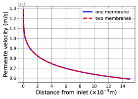
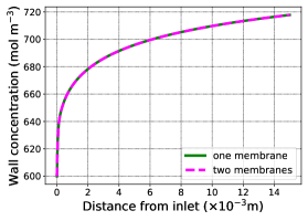
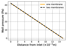
Figure 7.2: Example 7.2. Comparison along $\Gamma_{\mathrm{m}}$ between permeate velocities, concentration profiles and pressures between the two channel scenarios.

7.3 A channel with a spacer

In this test we study the behaviour of the proposed method when an obstacle, serving a a spacer, is considered. More precisely, we consider a channel with the same dimensions as the previous experiment, but with the addition of a spacer in the middle of the channel in a cavity-type configuration. The spacer corresponds to the cross section of a cylinder, i.e., a circle, with diameter $3.6\cdot 10^{-4}$m and tangent to the membrane. The boundary conditions for the spacer are the same as $\Gamma_{\mathrm{wall}}$. To study the behaviour of the method, the velocities to be tested in this experiment are $u_{0}=5\cdot 10^{-2}$m$/$s and $u_{0}=1.29\cdot 10^{-1}$m$/$s, and the effect of the salt concentration boundary layer along the membrane is studied.

In Figure 7.3 we observe velocity and concentration profiles when different inlet velocities are considered. The flow exhibits recirculating zones caused by the spacer, inducing an accumulation of salt near the spacer. Moreover, near the tangent point we observe the maximum salt concentration. This is described in Figure 7.4, where we observe that the high velocity profile yields a lower concentration of salt along the membrane despite the higher recirculating zone. Also, the gauge pressure drop observed for the high velocity profile is more pronounced around the spacer boundary point, as expected.

$|\boldsymbol{u}_{h}|$

$\theta_{h}$  

Figure 7.3: Velocity streamlines (top panels) and concentration profiles (bottom panels) around the spacer in a cavity-type configuration and inlet velocities $u_{0}=5.0\cdot 10^{-2}$m$/$s (left) and $u_{0}=1.29\cdot 10^{-1}$m$/$s. The bottom numbers indicate distance from inlet (in $\times 10^{-3}$m).

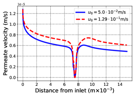
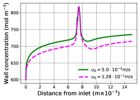
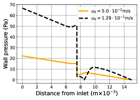
Figure 7.4: Example 7.3. Comparison along $\Gamma_{\mathrm{m}}$ between permeate velocities, concentration profiles and pressures between the two velocities scenarios in the channel with cavity-type spacer configurations.

Appendix A Lagrange multiplier stabilisation for a conforming approximation

We report on experiments performed using the $\boldsymbol{\mathrm{H}}$-conforming stabilised scheme with Lagrange multipliers proposed in [41]. We test different stabilised schemes based on $\mathbb{P}_{0}$ and discontinuous $\mathbb{P}_{1}$ for the Lagrange multiplier.

DoF	$h$	$\mathrm{e}(\boldsymbol{u})$	$r(\boldsymbol{u})$	$\mathrm{e}(p)$	$r(p)$	$\mathrm{e}(\lambda)$	$r(\lambda)$	$\mathrm{e}(\theta)$	$r(\theta)$	it
No stabilisation
86	0.707	6.67e-01	$\star$	1.86e-01	$\star$	9.15e-02	$\star$	2.78e-02	$\star$	7
166	0.471	3.14e-01	1.86	5.24e-02	3.13	2.73e-02	2.99	1.12e-02	2.25	7
404	0.283	1.18e-01	1.92	1.07e-02	3.11	8.38e-03	2.31	3.81e-03	2.11	7
1192	0.157	3.71e-02	1.96	2.15e-03	2.74	2.93e-03	1.79	1.15e-03	2.04	7
4016	0.083	1.05e-02	1.99	5.09e-04	2.26	1.07e-03	1.59	3.20e-04	2.01	7
14656	0.043	2.80e-03	1.99	1.32e-04	2.04	3.82e-04	1.55	8.50e-05	2.00	7
Stabilisation with $\alpha_{0}=0.1,\,\delta=-1$
86	0.707	6.91e-01	$\star$	3.66e-01	$\star$	3.26e-01	$\star$	3.18e-02	$\star$	6
166	0.471	3.18e-01	1.91	1.06e-01	3.06	9.40e-02	3.07	1.19e-02	2.43	7
404	0.283	1.18e-01	1.94	2.13e-02	3.14	2.03e-02	3.00	3.85e-03	2.20	7
1192	0.157	3.72e-02	1.97	3.59e-03	3.04	4.26e-03	2.65	1.15e-03	2.05	7
4016	0.083	1.05e-02	1.99	6.36e-04	2.72	1.07e-03	2.17	3.20e-04	2.01	7
14656	0.043	2.80e-03	1.99	1.39e-04	2.30	3.29e-04	1.79	8.51e-05	2.00	7
Stabilisation with $\alpha_{0}=0.1,\,\delta=0$
86	0.707	6.68e-01	$\star$	2.06e-01	$\star$	1.45e-01	$\star$	2.76e-02	$\star$	7
166	0.471	3.14e-01	1.86	5.65e-02	3.20	3.56e-02	3.47	1.12e-02	2.23	7
404	0.283	1.18e-01	1.92	1.14e-02	3.13	8.86e-03	2.72	3.81e-03	2.10	7
1192	0.157	3.71e-02	1.96	2.23e-03	2.78	2.67e-03	2.04	1.15e-03	2.04	7
4016	0.083	1.05e-02	1.99	5.21e-04	2.29	9.06e-04	1.70	3.20e-04	2.01	7
14656	0.043	2.80e-03	1.99	1.34e-04	2.04	3.13e-04	1.60	8.50e-05	2.00	7
Stabilisation with $\alpha_{0}=0.1,\,\delta=1$
86	0.707	6.63e-01	$\star$	1.66e-01	$\star$	8.23e-02	$\star$	2.72e-02	$\star$	7
166	0.471	3.13e-01	1.85	4.55e-02	3.19	2.23e-02	3.22	1.11e-02	2.21	7
404	0.283	1.18e-01	1.92	9.64e-03	3.04	7.08e-03	2.25	3.81e-03	2.10	7
1192	0.157	3.71e-02	1.96	2.07e-03	2.61	2.44e-03	1.81	1.15e-03	2.04	7
4016	0.083	1.05e-02	1.98	5.20e-04	2.17	8.75e-04	1.61	3.20e-04	2.01	7
14656	0.043	2.80e-03	1.99	1.36e-04	2.02	3.09e-04	1.57	8.50e-05	2.00	7

Table A.1: Example A. Error history for a finite element family with $\mathbb{P}^{2}_{2}-\mathbb{P}_{1}-\mathbb{P}_{0}-\mathbb{P}_{2}$ for $\boldsymbol{u}_{h},p_{h},\lambda_{h}$ and $\theta_{h}$, respectively. For this case the Lagrange multiplier errors are measured in the $\mathrm{H}^{-1/2}(\Gamma_{\mathrm{m}})-$norm.

In the conforming case, the discrete inf-sup condition to be satisfied is given by

$$\sup_{\boldsymbol{v}_{h}\in\boldsymbol{\mathrm{H}}_{h},\boldsymbol{v}_{h}\neq\boldsymbol{0}}\frac{b_{h}(\boldsymbol{v}_{h},(q_{h},\xi_{h}))}{\|\boldsymbol{v}_{h}\|_{1,\Omega}}\gtrsim\|q_{h}\|_{0,\Omega}+\|\xi_{h}\|_{-1/2,\Gamma_{\mathrm{m}}}\quad\forall(q_{h},\xi_{h})\in Q_{h}\times W_{h}.$$

However, in [41] it is shown that despite choosing stable inf-sup elements such as Taylor–Hood, Mini-element, $\mathbb{P}_{2}-\mathbb{P}_{0}$, etc, together with a typical choice for the Lagrange multiplier space as above, this condition may not be satisfied. To circumvent this difficulty, one can either enrich the velocity space with bubbles having compact support along $\Gamma_{\mathrm{m}}$ (see [41] for details), or add suitable residual stabilisation in the discrete problem (see, for example [42, 40]). We adopt the latter option. We define generic finite element spaces $\boldsymbol{\mathrm{H}}_{h}\subset\boldsymbol{\mathrm{H}}$, $Q_{h}\subset Q$, $W_{h}\subset W$ and $Z_{h}\subset Z$ for the velocity, pressure, Lagrange multiplier, and concentration, respectively. Following [40], we first define the following mesh-dependent bilinear form $d_{h}:W_{h}\times W_{h}\to\mathbb{R}$:

(46) $$d_{h}(\lambda_{h},\xi_{h}):=\sum_{e\in\mathcal{E}_{\mathrm{m}}}h_{e}\int_{e}\lambda_{h}\,\xi_{h}\,\mathrm{d}s,\qquad\forall\lambda_{h},\xi_{h}\in W_{h}.$$

The resulting stabilised formulation consists in finding $(\boldsymbol{u}_{h},p_{h},\lambda_{h},\theta_{h})\in\boldsymbol{\mathrm{H}}_{h}\times Q_{h}\times W_{h}\times Z_{h}$ such that

(47) $$a(\boldsymbol{u}_{h},\boldsymbol{v}_{h})+\widetilde{a}(\boldsymbol{u}_{h};\boldsymbol{u}_{h},\boldsymbol{v}_{h})+b(\boldsymbol{v}_{h},(p_{h},\lambda_{h}))+s_{1}((\boldsymbol{u}_{h},p_{h},\lambda_{h}),\boldsymbol{v}_{h}) =0,$$

$$b(\boldsymbol{u}_{h},(q_{h},\xi_{h}))+s_{2}((\boldsymbol{u}_{h},p_{h},\lambda_{h}),(q_{h},\xi_{h})) =\langle\xi_{h},g(\theta_{h})\rangle_{\Gamma_{\mathrm{m}}},$$

$$c(\theta_{h},\tau_{h})+\widetilde{c}(\boldsymbol{u}_{h};\theta_{h},\tau_{h}) =0,$$

for all $(\boldsymbol{v}_{h},q_{h},\xi_{h},\tau_{h})\in\boldsymbol{\mathrm{H}}_{h}\times Q_{h}\times W_{h}\times Z_{h}$, where the stabilising bilinear forms are

$$s_{1}((\boldsymbol{u}_{h},p_{h},\xi_{h}),\boldsymbol{v}_{h}) =-\alpha_{0}d_{h}\bigl{(}\xi_{h}+(\boldsymbol{\sigma}_{h}\boldsymbol{n})\cdot\boldsymbol{n},\delta\mu_{0}(\nabla\boldsymbol{v}_{h}\boldsymbol{n})\cdot\boldsymbol{n}\bigr{)},$$

$$s_{2}((\boldsymbol{u}_{h},p_{h},\xi_{h}),(q_{h},\chi_{h})) =-\alpha_{0}d_{h}\bigl{(}\xi_{h}+(\boldsymbol{\sigma}_{h}\boldsymbol{n})\cdot\boldsymbol{n},\chi_{h}-\delta(q_{h}\mathbb{I}\boldsymbol{n})\cdot\boldsymbol{n}\bigr{)}.$$

Note that for the conforming method, the discrete quantities $\xi_{h},\,\boldsymbol{\sigma}_{h}\boldsymbol{n}\cdot\boldsymbol{n},\,\nabla\boldsymbol{v}_{h}\boldsymbol{n}\cdot\boldsymbol{n},\,q_{h}\mathbb{I}\boldsymbol{n}\cdot\boldsymbol{n}$ all belong to $W_{h}$. Note also that, for a Navier–Stokes model with slip boundary condition, [42] proved that choosing $\delta=0$ and $\alpha_{0}$ lower than a threshold yields a stable method. As in [23], for $\delta=1$ we have symmetry, however a smallness condition on $\alpha_{0}$ is needed for sake of stability. For $\delta=-1$ we have the anti-symmetric variation of the method [16, 4], whose main advantage is the unconditional stability with respect to $\alpha_{0}$.

First let us consider the same domain and exact solution as in Test 7.1 and study the convergence of the conforming scheme using Taylor–Hood elements together with piecewise linear or constant discontinuous elements for the Lagrange multiplier. We also consider stabilised and non-stabilised formulations in order to test the robustness of the scheme.

DoF	$h$	$\mathrm{e}(\boldsymbol{u})$	$r(\boldsymbol{u})$	$\mathrm{e}(p)$	$r(p)$	$\mathrm{e}(\lambda)$	$r(\lambda)$	$\mathrm{e}(\theta)$	$r(\theta)$	it
No stabilisation
88	0.707	6.72e-01	$\star$	2.57e-01	$\star$	1.98e-01	$\star$	2.71e-02	$\star$	7
169	0.471	3.16e-01	1.86	7.16e-02	3.15	1.20e-01	1.24	1.11e-02	2.21	7
409	0.283	1.19e-01	1.91	1.39e-02	3.20	1.30e-01	-0.16	3.80e-03	2.09	7
1201	0.157	3.80e-02	1.94	2.58e-03	2.87	9.67e-02	0.50	1.15e-03	2.04	7
4033	0.083	1.10e-02	1.95	5.42e-04	2.45	6.38e-02	0.65	3.20e-04	2.01	7
14689	0.043	3.05e-03	1.93	1.29e-04	2.16	4.13e-02	0.66	8.51e-05	2.00	7
Stabilisation with $\alpha_{0}=0.1,\,\delta=-1$
88	0.707	7.06e-01	$\star$	3.87e-01	$\star$	2.71e-01	$\star$	9.54e-02	$\star$	6
169	0.471	3.30e-01	1.88	1.23e-01	2.84	2.17e-01	0.55	3.71e-02	2.33	7
409	0.283	1.25e-01	1.89	6.04e-02	1.39	1.06e-01	1.41	1.31e-02	2.04	7
1201	0.157	3.99e-02	1.95	2.20e-02	1.72	3.69e-02	1.79	4.02e-03	2.01	7
4033	0.083	1.13e-02	1.98	6.53e-03	1.91	1.09e-02	1.92	1.12e-03	2.00	7
14689	0.043	3.01e-03	1.99	1.77e-03	1.97	2.94e-03	1.97	2.98e-04	2.00	7
Stabilisation with $\alpha_{0}=0.1,\,\delta=0$
88	0.707	6.99e-01	$\star$	3.16e-01	$\star$	6.85e-01	$\star$	8.45e-02	$\star$	6
169	0.471	3.32e-01	1.83	1.53e-01	1.78	3.66e-01	1.55	3.64e-02	2.08	7
409	0.283	1.26e-01	1.90	6.70e-02	1.62	1.39e-01	1.89	1.31e-02	2.00	7
1201	0.157	3.99e-02	1.95	2.29e-02	1.83	4.27e-02	2.01	4.02e-03	2.01	7
4033	0.083	1.13e-02	1.98	6.63e-03	1.95	1.17e-02	2.03	1.12e-03	2.00	7
14689	0.043	3.02e-03	1.99	1.78e-03	1.98	3.06e-03	2.03	2.98e-04	2.00	7
Stabilisation with $\alpha_{0}=0.1,\,\delta=1$
88	0.707	7.29e-01	$\star$	5.21e-01	$\star$	1.00e+00	$\star$	8.25e-02	$\star$	6
169	0.471	3.40e-01	1.88	2.14e-01	2.19	4.70e-01	1.87	3.64e-02	2.02	7
409	0.283	1.27e-01	1.92	7.78e-02	1.98	1.66e-01	2.04	1.31e-02	2.00	7
1201	0.157	4.01e-02	1.97	2.41e-02	1.99	4.74e-02	2.13	4.02e-03	2.01	7
4033	0.083	1.13e-02	1.99	6.75e-03	2.00	1.24e-02	2.11	1.13e-03	2.00	7
14689	0.043	3.02e-03	1.99	1.79e-03	2.00	3.15e-03	2.07	2.99e-04	2.00	7

Table A.2: Example A. Error history for a finite element family with $\mathbb{P}^{2}_{2}-\mathbb{P}_{1}-\mathbb{P}_{1}-\mathbb{P}_{2}$ for $\boldsymbol{u}_{h},p_{h},\lambda_{h}$ and $\theta_{h}$, respectively. For this case the Lagrange multiplier errors are measured in the $\mathrm{H}^{-1/2}(\Gamma_{\mathrm{m}})-$norm.

The numerical results portrayed in Tables A.1–A.2 clearly confirm the theoretical $O(h^{k+1})$-convergence in the energy norm similarly to the observed/predicted in [42, 40]. The blocks in Table A.1 show the error history displaying number of degrees of freedom, individual absolute errors, rates of convergence, and Newton iteration counts for the conforming discretisation using Taylor–Hood approximation of velocity-pressure, together with piecewise discontinuous elements for the Lagrange multiplier (on a submesh conforming with the bulk mesh), and piecewise quadratic and continuous functions for the concentration. However, the choice of $\mathbb{P}_{0}$ for the Lagrange multiplier shows an experimental rate of $\mathcal{O}(h^{1.5})$ for all the cases.

On the other hand, the results of using linear discontinuous elements, presented in Table A.2 show a noticeable deterioration of the convergence for the Lagrange multiplier when the stabilisation is removed. In turn, an optimal rate of convergence $O(h^{k+1})$ is achieved with stabilisation.

Appendix B Divergence-free non-conforming test

Finally, we use the lowest-order Crouzeix–Raviart elements ($\mathbb{CR}_{1}-\mathbb{P}_{0}$ for velocity-pressure pairs), characterised by velocities being nonconforming with $\boldsymbol{\mathrm{H}}^{1}(\Omega)$ instead of the div-free pair $\mathbb{BDM}_{1}-\mathbb{P}_{0}$. In addition, we use piecewise constants to approximate the Lagrange multiplier. Table B.1 describes the behaviour of the scheme with a stabilisation parameter $\alpha_{0}=20$, indicating a similar accuracy as in the $\boldsymbol{\mathrm{H}}^{1}(\Omega)$-conforming scheme presented in Table 7.1.

DoF	$h$	$\mathrm{e}(\boldsymbol{u})$	$r(\boldsymbol{u})$	$\mathrm{e}(p)$	$r(p)$	$\mathrm{e}(\lambda)$	$r(\lambda)$	$\mathrm{e}(\theta)$	$r(\theta)$	it
Stabilisation using $\mathbb{CR}_{1}-\mathbb{P}_{0},\,\alpha_{0}=20$
971	0.141	4.14e-01	$\star$	2.24e+00	$\star$	1.35e+00	$\star$	3.64e-02	$\star$	7
3741	0.071	1.99e-01	1.06	1.19e+00	0.91	7.24e-01	0.90	1.82e-02	1.00	7
8311	0.047	1.31e-01	1.04	8.05e-01	0.96	4.91e-01	0.96	1.21e-02	1.00	7
14681	0.035	9.73e-02	1.02	6.08e-01	0.97	3.70e-01	0.98	9.06e-03	1.00	7
22851	0.028	7.76e-02	1.01	4.89e-01	0.98	2.96e-01	0.99	7.24e-03	1.00	7
32821	0.024	6.45e-02	1.01	4.08e-01	0.99	2.47e-01	1.00	6.03e-03	1.00	7

Table B.1: Example B. Error history for a finite element family with $\mathbb{CR}_{1}-\mathbb{P}_{0}-\mathbb{P}_{0}-\mathbb{P}_{1}$ for $\boldsymbol{u}_{h},p_{h},\lambda_{h}$ and $\theta_{h}$, respectively. For this case the Lagrange multiplier errors are measured in the $\mathrm{H}^{-1/2}(\Gamma_{\mathrm{m}})-$norm..

References

• [1] M. Alnæs, J. Blechta, J. Hake, A. Johansson, B. Kehlet, A. Logg, C. Richardson, J. Ring, M. E. Rognes, and G. N. Wells, The FEniCS project version 1.5, Archive of Numerical Software, 3 (2015).
• [2] R. Arndt, A. N. Ceretani, and C. N. Rautenberg, On existence and uniqueness of solutions to a Boussinesq system with nonlinear and mixed boundary conditions, Journal of Mathematical Analysis and Applications, 490 (2020), p. 124201.
• [3] S. Badia, M. Hornkjol, A. Khan, K.-A. Mardal, A. F. Martín, and R. Ruiz-Baier, Efficient and reliable divergence-conforming methods for an elasticity-poroelasticity interface problem, Computers & Mathematics with Applications, 157 (2024), pp. 173–194.
• [4] H. J. Barbosa and T. J. Hughes, Boundary Lagrange multipliers in finite element methods: error analysis in natural norms, Numerische Mathematik, 62 (1992), pp. 1–15.
• [5] B. Bernales, P. Haldenwang, P. Guichardon, and N. Ibaseta, Prandtl model for concentration polarization and osmotic counter-effects in a 2-d membrane channel, Desalination, 404 (2017), pp. 341–359.
• [6] H. Brezis, Functional analysis, Sobolev spaces and partial differential equations, vol. 2, Springer, 2011.
• [7] F. Brezzi and M. Fortin, Variational formulations and finite element methods, Mixed and hybrid finite element methods, (1991), pp. 1–35.
• [8] A. Buffa and C. Ortner, Compact embeddings of broken sobolev spaces and applications, IMA journal of numerical analysis, 29 (2009), pp. 827–855.
• [9] R. Bürger, P. E. Méndez, and R. Ruiz-Baier, On H(div)-conforming methods for double-diffusion equations in porous media, SIAM Journal on Numerical Analysis, 57 (2019), pp. 1318–1343.
• [10] N. Carro, D. Mora, and J. Vellojin, A finite element model for concentration polarization and osmotic effects in a membrane channel, To appear in International Journal for Numerical Methods in Fluids, (2024).
• [11] A. N. Ceretani and C. N. Rautenberg, The Boussinesq system with mixed non-smooth boundary conditions and do-nothing boundary flow, Zeitschrift für angewandte Mathematik und Physik, 70 (2019), p. 14.
• [12] B. Cockburn, G. Kanschat, and D. Schötzau, A note on discontinuous galerkin divergence-free solutions of the navier–stokes equations, Journal of Scientific Computing, 31 (2007), pp. 61–73.
• [13] P.-H. Cocquet, M. Rakotobe, D. Ramalingom, and A. Bastide, Error analysis for the finite element approximation of the darcy–brinkman–forchheimer model for porous media with mixed boundary conditions, Journal of Computational and Applied Mathematics, 381 (2021), p. 113008.
• [14] C. Ebmeyer and J. Frehse, Steady Navier-Stokes equations with mixed boundary value conditions in three-dimensional Lipschitzian domains, Mathematische Annalen, 319 (2001), pp. 349–381.
• [15] A. Ern and J.-L. Guermond, Applied mathematical sciences, Theory and Practice of Finite Elements, 159 (2004).
• [16] L. P. Franca and R. Stenberg, Error analysis of galerkin least squares methods for the elasticity equations, SIAM Journal on Numerical Analysis, 28 (1991), pp. 1680–1697.
• [17] G. N. Gatica, A simple introduction to the mixed finite element method, Theory and Applications. Springer Briefs in Mathematics. Springer, London, (2014).
• [18] G. N. Gatica, G. C. Hsiao, and S. Meddahi, Further developments on boundary-field equation methods for nonlinear transmission problems, Journal of Mathematical Analysis and Applications, 502 (2021), p. 125262.
• [19] V. Girault and P.-A. Raviart, Finite Element Approximation of the Navier-Stokes equations, vol. 749, Springer Berlin, 1979.
• [20] C. Greif, D. Li, D. Schötzau, and X. Wei, A mixed finite element method with exactly divergence-free velocities for incompressible magnetohydrodynamics, Computer Methods in Applied Mechanics and Engineering, 199 (2010), pp. 2840–2855.
• [21] P. Grisvard, Elliptic problems in nonsmooth domains, SIAM, 2011.
• [22] P. Hansbo and M. G. Larson, Discontinuous galerkin methods for incompressible and nearly incompressible elasticity by nitsche’s method, Computer Methods in Applied Mechanics and Engineering, 191 (2002), pp. 1895–1908.
• [23] T. J. Hughes, L. P. Franca, and G. M. Hulbert, A new finite element formulation for computational fluid dynamics: Viii. the galerkin/least-squares method for advective-diffusive equations, Computer methods in applied mechanics and engineering, 73 (1989), pp. 173–189.
• [24] R. Ingram, Finite Element Approximation of nonsolenoidal, viscous flows around porous and solid obstacles, SIAM Journal on Numerical Analysis, 49 (2011), pp. 491–520.
• [25] V. John, A. Linke, C. Merdon, M. Neilan, and L. G. Rebholz, On the divergence constraint in mixed finite element methods for incompressible flows, SIAM review, 59 (2017), pp. 492–544.
• [26] T. Kashiwabara, I. Oikawa, and G. Zhou, Penalty method with P1/P1 finite element approximation for the Stokes equations under the slip boundary condition, Numerische Mathematik, 134 (2016), pp. 705–740.
• [27]  , Penalty method with crouzeix–raviart approximation for the stokes equations under slip boundary condition, ESAIM: Mathematical Modelling and Numerical Analysis, 53 (2019), pp. 869–891.
• [28] T. Kim, Steady Boussinesq system with mixed boundary conditions including friction conditions, Applications of Mathematics, 67 (2022), pp. 593–613.
• [29] M. Kuchta, Assembly of multiscale linear PDE operators, in Numerical Mathematics and Advanced Applications ENUMATH 2019: European Conference, Egmond aan Zee, The Netherlands, September 30-October 4, Springer, 2020, pp. 641–650.
• [30] W. Layton, Weak imposition of “no-slip” conditions in finite element methods, Computers & Mathematics with Applications, 38 (1999), pp. 129–142.
• [31] C. Le Roux and B. Reddy, The steady Navier-Stokes equations with mixed boundary conditions: application to free boundary flows, Nonlinear Analysis: Theory, Methods & Applications, 20 (1993), pp. 1043–1068.
• [32] A. Liakos, Discretization of the Navier–Stokes equations with slip boundary condition, Numerical Methods for Partial Differential Equations: An International Journal, 17 (2001), pp. 26–42.
• [33] S. A. Lorca and J. L. Boldrini, The initial value problem for a generalized Boussinesq model, Nonlinear Analysis, 36 (1999), pp. 457–480.
• [34] J. Luo, M. Li, and Y. Heng, A hybrid modeling approach for optimal design of non-woven membrane channels in brackish water reverse osmosis process with high-throughput computation, Desalination, 489 (2020), p. 114463.
• [35] A. Manzoni, A. Quarteroni, and S. Salsa, A saddle point approach to an optimal boundary control problem for steady Navier-Stokes equations, Mathematics in Engineering, 1 (2019), pp. 252–280.
• [36] K. G. Nayar, M. H. Sharqawy, L. D. Banchik, et al., Thermophysical properties of seawater: A review and new correlations that include pressure dependence, Desalination, 390 (2016), pp. 1–24.
• [37] R. Oyarzúa, T. Qin, and D. Schötzau, An exactly divergence-free finite element method for a generalized Boussinesq problem, IMA Journal of Numerical Analysis, 34 (2014), pp. 1104–1135.
• [38] P. W. Schroeder and G. Lube, Stabilised dG-FEM for incompressible natural convection flows with boundary and moving interior layers on non-adapted meshes, Journal of Computational Physics, 335 (2017), pp. 760–779.
• [39] R. Temam, Navier-Stokes equations: theory and numerical analysis, vol. 343, American Mathematical Soc., 2001.
• [40] J. M. Urquiza, A. Garon, and M.-I. Farinas, Weak imposition of the slip boundary condition on curved boundaries for Stokes flow, Journal of Computational Physics, 256 (2014), pp. 748–767.
• [41] R. Verfürth, Finite Element Approximation on incompressible Navier-Stokes equations with slip boundary condition, Numerische Mathematik, 50 (1986), pp. 697–721.
• [42] R. Verfürth, Finite Element Approximation of incompressible Navier-Stokes equations with slip boundary condition II, Numerische Mathematik, 59 (1991), pp. 615–636.
• [43] G. Zhou, T. Kashiwabara, and I. Oikawa, Penalty method for the stationary Navier–Stokes problems under the slip boundary condition, Journal of Scientific Computing, 68 (2016), pp. 339–374.