Guidance Graph Optimization for Lifelong Multi-Agent Path Finding

Abstract

We study how to use guidance to improve the throughput of lifelong Multi-Agent Path Finding (MAPF). Previous studies have demonstrated that while incorporating guidance, such as highways, can accelerate MAPF algorithms, this often results in a trade-off with solution quality. In addition, how to generate good guidance automatically remains largely unexplored, with current methods falling short of surpassing manually designed ones. In this work, we introduce the directed guidance graph as a versatile representation of guidance for lifelong MAPF, framing Guidance Graph Optimization (GGO) as the task of optimizing its edge weights. We present two GGO algorithms to automatically generate guidance for arbitrary lifelong MAPF algorithms and maps. The first method directly solves GGO by employing CMA-ES, a black-box optimization algorithm. The second method, PIU, optimizes an update model capable of generating guidance, demonstrating the ability to transfer optimized guidance graphs to larger maps with similar layouts. Empirically, we show that (1) our guidance graphs improve the throughput of three representative lifelong MAPF algorithms in four benchmark maps, and (2) our update model can generate guidance graphs for as large as $93\times 91$ maps and as many as 3000 agents.

1 Introduction

We study the problem of leveraging a guidance graph with optimized edge weights to guide agent movement, thereby improving the throughput of lifelong Multi-Agent Path Finding (MAPF). MAPF (Stern et al., 2019) involves planning collision-free paths for a set of agents from their start to goal locations on a given graph $G$. Lifelong MAPF (Li et al., 2021) extends MAPF by assigning new goals to agents as soon as they reach their current ones. Example applications include character control in video games (Ma et al., 2017b; Jansen and Sturtevant, 2008) and automated warehouses in which hundreds of robots are continually assigned new tasks to transport inventory pods (Varambally et al., 2022). Driven by these real-world demands, numerous studies have focused on improving the throughput, namely the average number of reached goals per timestep, by developing better lifelong MAPF algorithms (Ma et al., 2017a; Li et al., 2020; Kou et al., 2020; Damani et al., 2021) or optimizing map layouts (i.e., map structures) (Zhang et al., 2023a, b).

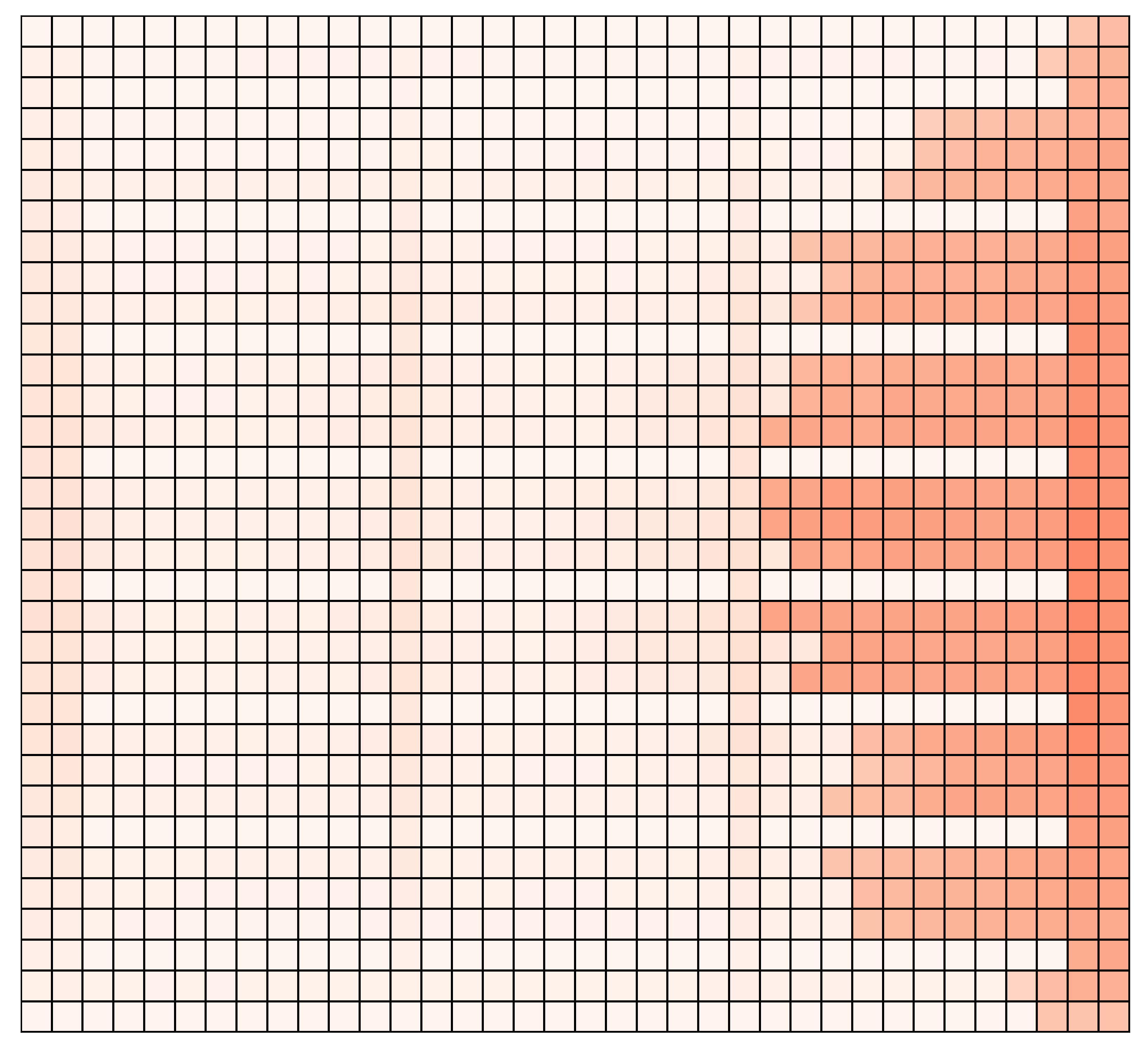
(a) No guidance

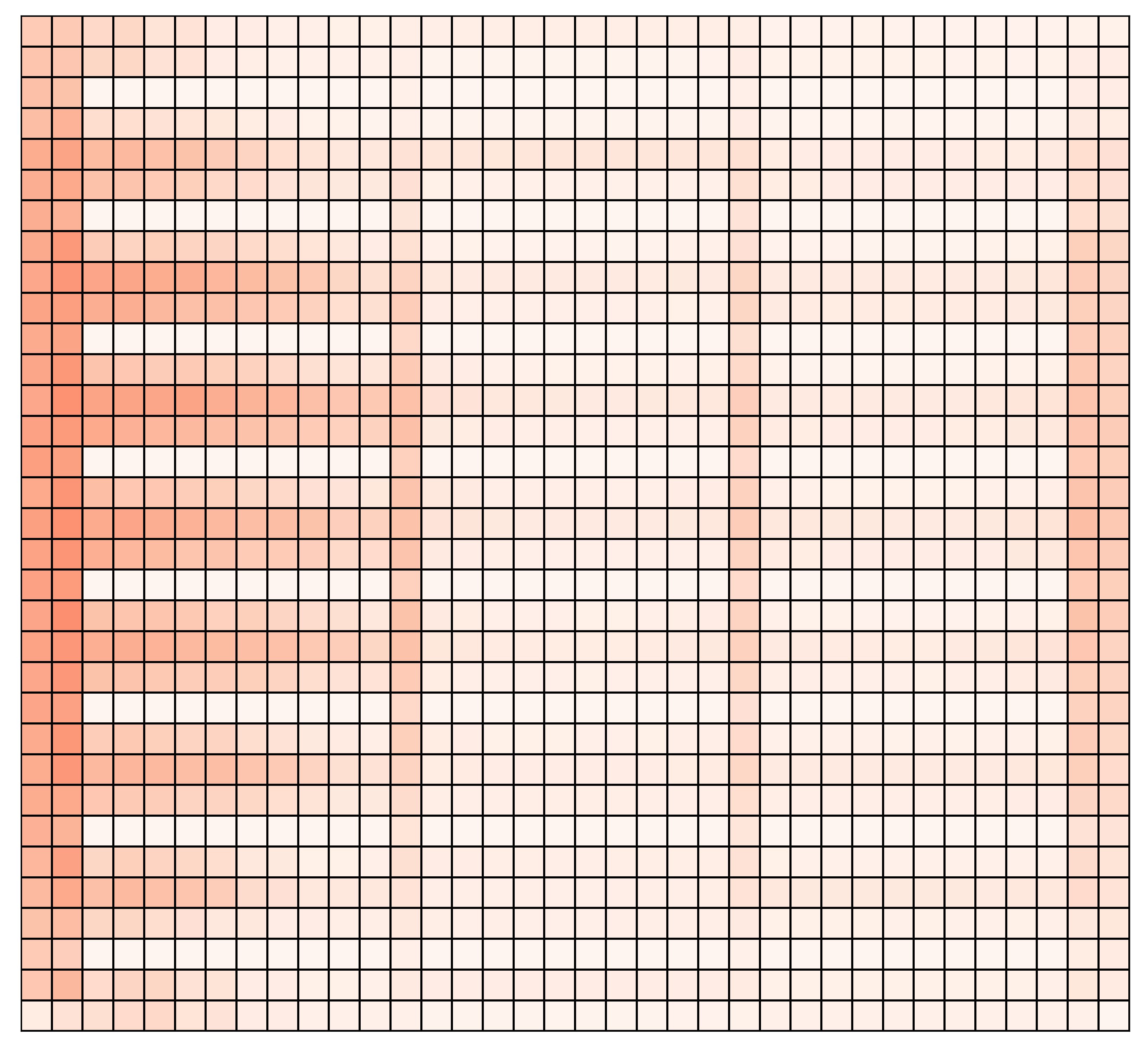
(b) Crisscross

(c) Our guidance

Figure 1: Comparison of no guidance, human-designed crisscross guidance, and our guidance with a simulation of 240 agents in a 33 $\times$ 36 warehouse map, shown in Figure 8(b) in Appendix B. The heatmaps show the tile-usage (the frequency that each tile is occupied). Our guidance results in the most balanced traffic with the highest throughput.

Given that lifelong MAPF requires online computation of new paths as agents are continuously assigned to new goal locations, lifelong MAPF algorithms always decompose the problem into a series of (one-shot) MAPF instances and solve them sequentially. However, such methods are myopic because each MAPF instance involves only the current goal locations. Achieving (near-)optimal solutions for individual MAPF instances does not necessarily result in the best throughput. In this work, we propose to foster implicit cooperation among agents over the long term by introducing global guidance for agent movement. Our guidance takes the form of a directed weighted graph that alters the costs of agents moving along each edge and waiting at each vertex of graph $G$. Intuitively, such a guidance graph serves two purposes. First, by amplifying the cost difference of traveling through an edge in opposite directions, we encourage agents to move in the same direction, reducing the number of head-on collisions, which happen when two agents try to traverse through the same edge in opposite directions. Second, by increasing the cost of moving in areas prone to congestion, we motivate agents to navigate through less congested areas, ultimately reducing traffic congestion. Figure 1 shows the tile-usage resulting from different guidance strategies.

One closely related work to our guidance graph is highways (Cohen et al., 2015; Li and Sun, 2023), which are a subset of edges selected from graph $G$ with assigned directions and a lower traversal cost. This strategy incentivizes agents to move along the highways, reducing the number of collisions to be resolved by MAPF algorithms. However, the question of how to select these edges and determine their directions and costs remains largely unexplored. The crisscross approach (Cohen, 2020), where edge directions alternate in even and odd rows and columns, is common but not optimal; Li and Sun (2023) show that, while crisscross highways speed up lifelong MAPF algorithms, they do not always improve throughput. Additionally, Cohen et al. (2016a) proposed two methods to select edges and directions for highways, but neither of them outperforms crisscross highways.

Therefore, we introduce the Guidance Graph Optimization (GGO) problem to improve throughput by optimizing the edge weights of a directed guidance graph. We present two automatic GGO methods. The first applies Covariance Matrix Adaptation Evolutionary Strategy (CMA-ES) (Hansen, 2016), a state-of-the-art black-box optimizer, to solve GGO, but its solution is map-specific. Therefore, we propose the second method, Parameterized Iterative Update (PIU), which uses CMA-ES to optimize an update model. This update model, represented by a neural network, starts with an unweighted guidance graph and iteratively updates it with traffic information obtained from a lifelong MAPF simulator. It is capable of optimizing guidance graphs for different maps with similar layouts.

We make the following contributions: (1) introducing the guidance graph, a versatile representation of guidance for lifelong MAPF, and guidance graph optimization (GGO) to improve its throughput, (2) conducting an in-depth study of various existing guidance works in MAPF, and (3) proposing two automatic GGO methods, CMA-ES and PIU, showcasing their superior performance over unweighted graphs and previous guidance methods, along with the transferability of PIU to larger maps with similar layouts.

2 Problem Definition and Preliminaries

2.1 Lifelong Multi-Agent Path Finding

Definition 1 ((One-Shot) MAPF).

The (one-shot) MAPF problem takes as inputs a graph $G(V,E)$ and $k$ agents $A=\{a_{1},..,a_{k}\}$ with their start and goal locations. At each timestep, an agent can move to an adjacent vertex or stay at its current vertex. Two agents collide when they arrive at the same vertex or swap locations at the same timestep. The (one-shot) MAPF problem searches for collision-free paths that move each agent $a_{i}$ from their start to goal locations with minimal sum-of-cost, defined as the total number of actions the agents need to take.

Definition 2 (Lifelong MAPF).

Lifelong MAPF extends one-shot MAPF by constantly assigning new goals to agents when they reach their current ones. Lifelong MAPF searches for collision-free paths that maximize throughput, namely the average number of reached goals per timestep.

2.1.1 Lifelong MAPF Algorithms

Solving MAPF optimally is known to be NP-hard (Yu and LaValle, 2013). Lifelong MAPF poses an even greater challenge as agents consistently receive new goal locations, requiring the continuous computation of new paths. Consequently, state-of-the-art algorithms approach lifelong MAPF by decomposing it into a series of (modified) one-shot MAPF instances, usually one at each timestep, assuming that minimizing their sum-of-costs enhances lifelong MAPF throughput. They can be divided into three categories. To show the generality of our GGO algorithms, we select a leading algorithm from each category to conduct our experiments.

Replan all. We replan all agents at every timestep (or every few timesteps) (Wan et al., 2018; Li et al., 2021). In each replanning cycle, we solve a MAPF instance with the start locations being the current locations of all agents and the goal locations being their current goal locations. We select RHCR (Li et al., 2021) as a representative algorithm from this category.

Replan new. This category is similar to the previous one except that we replan only agents that have just reached their current goal locations and have been assigned new goal locations at every timestep (Cáp et al., 2015; Ma et al., 2017a; Grenouilleau et al., 2019; Liu et al., 2019). Since agents being replanned must avoid collisions with agents not being replanned, methods in this category need to impose constraints on the map structure and goal locations, often denoted as well-formed maps, to ensure the existence of collision-free paths. We select DPP (Liu et al., 2019; Li et al., 2021) as a representative algorithm from this category.

Reactive. In contrast to the previous two categories, reactive methods plan paths for each agent without considering collisions with other agents (resulting in paths with no wait actions) and then resolve collisions reactively through pre-defined rules (Wang and Botea, 2008; Okumura et al., 2019; Yu and Wolf, 2023), such as inserting wait actions or taking short detours. We select PIBT Okumura et al. (2019) as a representative algorithm from this category. It is complete on biconnected graphs and runs significantly faster than algorithms in other categories.

		Representation			Generation			Usage
		Edge direction	Move cost	Wait cost	Design	MAPF	Online Update	Method
1	Jansen and Sturtevant (2008)	soft	$\mathbb{R^{+}}$	N/A	handcrafted procedure	lifelong	Yes	reactive
2	Wang and Botea (2008)	strict	1	N/A	crisscross	one-shot	No	reactive
3	Cohen et al. (2015)	soft	$\{1,c\}$	1	crisscross	one-shot	No	ECBS
4	Cohen et al. (2016b)	soft	$\{1,c\}$	1	handcrafted procedure	one-shot	No	ECBS
5	Li and Sun (2023)	soft	$\{1,c\}$	1	crisscross	lifelong	No	RHCR
6	Yu and Wolf (2023)	soft	$\mathbb{R^{+}}$	N/A	handcrafted procedure	lifelong	Yes	reactive
7	Chen et al. (2024)	soft	$\mathbb{R^{+}}$	N/A	handcrafted procedure	both	Yes	PIBT
8	GGO (ours)	soft	$\mathbb{R^{+}}$	$\mathbb{R^{+}}$	automatic	lifelong	No	many

Table 1: Overview of previous works on representation, generation, and usage of guidance in MAPF. For edge direction, strict means movement is unidirectional along each edge, and soft means bidirectional. Move cost refers to the cost of moving to an adjacent vertex and wait cost refers to the cost of waiting at the current vertex. For move cost, $\{1,c\}$ means that the value considers 1 and a scaler $c>1$ only. For design, handcrafted procedure refers to using a manually designed procedure to generate guidance, while crisscross refers to the popular human-designed guidance (Cohen, 2020).

2.2 Guidance Graph Optimization

To maintain generality, we consider graph $G(V,E)$ to be either directed, undirected, or mixed. We use $(u,v)$ and $(u\rightarrow v)$ to denote an undirected edge and a directed edge, respectively. We use $E_{und}$ and $E_{dir}$ to denote the subsets of edges in $E$ that are undirected and directed, respectively.

Definition 3 (Guidance Graph).

Given a graph $G(V,E)$ of a lifelong MAPF problem, we define a guidance graph as a directed weighted graph $G_{g}(V_{g},E_{g},\boldsymbol{\omega})$ with the same vertex set $V_{g}=V$. Each edge in $E_{g}$ corresponds to an action that an agent can take at each vertex, with the action cost represented by the edge weight. Formally, we define $E_{g}=E_{wait}\cup E_{move}$ such that

$$E_{wait} =\bigcup_{v\in V}\{(v\rightarrow v)\}$$ (1)

$$E_{move} =\{\bigcup_{(u,v)\in E_{und}}\{(u\rightarrow v),(v\rightarrow u)\}\}\cup E_{dir}.$$ (2)

All edges weights are collectively represented as a vector $\boldsymbol{\omega}\in\mathbb{R}^{|E_{g}|}_{>0}$.

Planinng with guidance graphs. To utilize guidance graphs in lifelong MAPF, we redefine the sum-of-costs of the underlying (one-shot) MAPF instances as the sum of the action costs across all paths for all agents (instead of the total number of actions). This leads to a minor modification to existing lifelong MAPF algorithms. Specifically, when planning paths for each agent, instead of seeking the shortest path on $G$, we aim to find a cost-minimal path on $G_{g}$. This modification alters the MAPF objective without compromising feasibility.

Definition 4 (Guidance Graph Optimization (GGO)).

Given an unweighted graph $G(V,E)$ of a lifelong MAPF problem, an objective function $f:\mathbb{R}^{|E_{g}|}\rightarrow\mathbb{R}$, as well as predefined lower and upper bounds $\boldsymbol{\omega_{lb}}$ and $\boldsymbol{\omega_{ub}}$ ($0<\boldsymbol{\omega_{lb}}\leq\boldsymbol{\omega_{ub}}$) for edge weights, the guidance graph optimization problem searches for the optimal guidance graph $G_{g}^{*}(V_{g},E_{g},\boldsymbol{\omega^{*}})$ with

$$\boldsymbol{\omega^{*}}=\operatorname*{arg\,max}_{\boldsymbol{\omega_{lb}}\leq\boldsymbol{\omega^{*}}\leq\boldsymbol{\omega_{ub}}}f(\boldsymbol{\omega}).$$ (3)

In this paper, our objective function $f$ is a simulator that runs a given lifelong MAPF algorithm on a given guidance graph and returns the throughput.

3 Guidance in MAPF

While the term “guidance” has not been explicitly proposed in the literature, the concept of enforcing global guidance and rules to enhance MAPF has been employed by numerous works in various ways. In this section, we present, for the first time, a summary of these works and provide a comprehensive review of how they represent, generate, and utilize guidance. Table 1 shows the comparison between them and our GGO. We will refer to them by their indices throughout the remainder of this section.

Representing Guidance. Previous works primarily represent guidance through modified edge directions or movement costs. They are all particular cases within the definition of the guidance graph, and none of them can represent varying wait costs. We roughly divide them into 4 categories. (1) Inspired by potential-field and flow-field methods used in swarm robotics, work 1 represents guidance through a direction map. This map assigns a direction vector to every vertex of $G$ and sets the movement cost along an edge to be inversely related to the dot product of its direction vector and the vector of the edge, encouraging agents to move along the direction vectors. Consequently, a direction map can be transformed into a guidance graph with edge weights defined as dot products mentioned above. (2) Work 2 turns some undirected edges into unidirectional, strictly prohibiting agents from moving against the assigned edge directions. This can be seen as a special guidance graph with infinite weights for constrained edges and 1 for others. (3) Works 3 to 5 use the highway idea that converts undirected edges into directed edges in both directions and then selects a subset of directed edges to be highways. They assign a weight of 1 for all highway edges and a weight of a predefined constant $c>1$ for other edges, encouraging agents to move along the highway edges. Highways are special guidance graphs with restrictions on the values of movement and wait costs. (4) Works 6 and 7 represent guidance similarly to our guidance graphs, with the distinction that they do not allow self-edges and thus cannot represent wait costs.

Generating Guidance. An important distinction between our work and previous works is that we are the first to propose an automated method for generating guidance. All previous works either use handcrafted guidance, such as crisscross highways (Works 2, 3, and 5), or use handcrafted procedures to generate guidance from a heatmap or a similar data structure that predicts traffic flows (Works 1, 4, 6, and 7). More specifically, Work 1 computes direction vectors (of the direction map) directly from past traffic flows and then uses a handcrafted equation to convert them into movement costs. Work 4 introduces two methods, GM and HM, for generating highways. GM uses a graphic model (Koller and Friedman, 2009) with a number of handcrafted features obtained from the estimated traffic flow. HM converts the estimated traffic flow into a score for each edge using a handcrafted score function and selects edges based on a predefined score threshold. Work 6 uses a data-driven model to predict traffic flow, or more specifically, the delays that the agents will encounter (due to collision avoidance etc.) and directly uses the predicted delays as movement costs. Last, Work 7 collects the planned paths of all agents and converts them into movement costs through a handcrafted equation.

Therefore, we select 4 baseline methods to generate guidance graphs in our experiments: (1) Unweighted, where no guidance is used, (2) Crisscross, (3) HM Cost, adapted from HM in Work 4, and (4) Traffic Flow, adapted from Work 7. We did not compare Work 1, as HM from Work 4 is inspired by it. We did not compare GM from Work 4, as its performance is similar to HM. We did not compare Work 6, because, while it obtains predicted traffic flow differently from Work 4, the procedure of converting predicted traffic flow to guidance is similar.

Please note that the HM Cost and Traffic Flow used in our experiments do not use the original traffic flow models in their papers. This is because Work 4 tackles one-shot MAPF and predicts traffic flows by planning shortest paths between the start and goal locations of the agents, which is not realistic in lifelong MAPF as goal locations are unknown in advance. Work 7 tackles lifelong MAPF but assumes the guidance graph can be updated on the fly using real-time traffic information, while we assume that our guidance graph is optimized offline, and thus we do not have access to real-time traffic information. Therefore, we use the same traffic flow model, namely the tile-usage map obtained from simulation, for both methods. More details can be found in Appendix A.

Using Guidance. All previous works study their guidance methods with a specific MAPF algorithm, so it remains unclear whether and how well their methods can generalize to other MAPF algorithms. For example, an evident limitation of methods designed for reactive (lifelong) MAPF algorithms (namely Works 1, 2, 6, and 7) is that, since paths planned by reactive methods do not include wait actions, these guidance methods, by design, do not define wait costs, making it non-trivial to extend them to (lifelong) MAPF algorithms in other categories. In contrast, we assess our GGO methods with three leading lifelong MAPF algorithms from different categories, thereby demonstrating their generality.

4 Approach

We first introduce CMA-ES to solve GGO directly. Then we introduce Parameterized Iterative Update (PIU), which uses CMA-ES to optimize an update model that iteratively generates a guidance graph based on simulated traffic information.

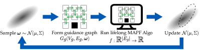
Figure 2: CMA-ES for GGO. The edge weights are iteratively sampled from a Gaussian distribution and then evaluated in a lifelong MAPF simulator. The simulated results are used to update the Gaussian distribution towards high-throughput regions.

4.1 CMA-ES

CMA-ES (Hansen, 2016) is a derivative-free, black-box, single-objective optimization algorithm based on covariance matrix adaptation. Figure 2 gives an overview of using CMA-ES to solve GGO. Specifically, we model the edge weights $\boldsymbol{\omega}$ as a multi-variate Gaussian distribution. We then iteratively sample from the distribution for new batches of edge weights, forming guidance graphs. We normalize the edge weights to be within a given bound $[\boldsymbol{\omega_{lb}},\boldsymbol{\omega_{ub}}]$. We then evaluate each guidance graph by running $N_{e\_cma}$ simulations in a given lifelong MAPF simulator and computing the average throughput. The evaluated guidance graphs are ranked based on the throughput and the top $N_{best}$ of them are used to update the Gaussian distribution towards the high-objective region of the search space. We run CMA-ES for $I$ iterations with batch size $b$. We return the guidance graph with the highest throughput as the solution.

Handling Bounds through Normalization. While optimizing the edge weights $\boldsymbol{\omega}$ directly, we need to handle the bound constraint. Yet, CMA-ES does not handle such bounds because the solutions are sampled from a Gaussian distribution.

We use min-max normalization to enforce the constraint because it does not affect path-planning solutions. To prove it, consider two guidance graphs with edge weights $\boldsymbol{\omega_{1}}$ and $\boldsymbol{\omega_{2}}=C\cdot\boldsymbol{\omega_{1}}$, where $C\in\mathbb{R^{+}}$. Since the weight of every edge is scaled by the same scaler $C$, the paths returned by the lifelong MAPF algorithms with low-level single agent solvers minimizing the sum of edge weights do not change. We show additional experiments in Appendix C that min-max normalization yields better solutions than representative bounds handling methods introduced by Biedrzycki (2020), which provides a comprehensive comparison of handle bounds methods for CMA-ES.

4.2 Parameterized Iterative Update

1

2

Input: $\mu_{0},\Sigma_{0}$: initial mean and covariance matrix of the multivariate Gaussian distribution.
$Np$: number of iterations to run in PIU. $update\_gaussian$: function to update $\mu$ and $\Sigma$ according to evaluated solutions.
$simulate$: function to run lifelong MAPF simulation and returns edge usage $U_{E_{g}}$ and wait action usage $U_{W}$.

3

4 Initialize $\mu\leftarrow\mu_{0},\Sigma\leftarrow\Sigma_{0},\boldsymbol{\theta^{*}}\leftarrow$ NULL $,g^{*}\leftarrow-\infty$

5 for $i\leftarrow 1$ to $I$ do

6       Sample $b$ solutions $\boldsymbol{\theta}_{1},...,\boldsymbol{\theta}_{b}\sim\mathcal{N}(\mu,\Sigma)$

7       for $k\leftarrow 1$ to $b$ do

8             $g_{k},\boldsymbol{\omega_{k}}\leftarrow$ PIU ($\boldsymbol{\theta}_{k},N_{p})$

9             if $g_{k}>g^{*}$ then

10                   $g^{*}\leftarrow g_{k},\boldsymbol{\theta^{*}}\leftarrow\boldsymbol{\theta_{k}}$

11                  

12            

13      $\mu,\Sigma\leftarrow update\_gaussian(g_{1\sim b},\boldsymbol{\theta_{1\sim b}})$

14      

15Return $g^{*},\boldsymbol{\theta^{*}}$

16 Function PIU ($\boldsymbol{\theta}$,$Np$):

17       Construct update model $\pi_{\boldsymbol{\theta}}$

18       Initialize $\boldsymbol{\omega}=\mathbf{1}$

19       for $j\leftarrow 1$ to $N_{p}$ do

20             Construct guidance graph $G_{g}(V_{g},E_{g},\boldsymbol{\omega})$

21             for $q\leftarrow 1$ to $N_{e\_piu}$ do

22                   $U_{E_{g}}^{(q)},f_{j}^{(q)}\leftarrow simulate(G_{g})$

23                  

24             $U_{E_{g}}\leftarrow\frac{1}{N_{e\_piu}}\sum_{q=1}^{N_{e\_piu}}U_{E_{g}}^{(q)}$

25             $f_{j}\leftarrow\frac{1}{N_{e\_piu}}\sum_{q=1}^{N_{e\_piu}}f_{j}^{(q)}$

26             $\boldsymbol{\omega}\leftarrow\pi_{\boldsymbol{\theta}}(\boldsymbol{\omega},U_{E_{g}})$

27            

28      Return $f_{N_{p}},\boldsymbol{\omega}$

29

Algorithm 1 Update model optimization

CMA-ES is known to scale poorly to high dimensional search spaces, make it challenging to optimize guidance graph for large maps. Therefore, we propose Parameterized Iterative Update (PIU). Figure 3 gives an overview the algorithm and Algorithm 1 provides the pseudocode. On a high level, PIU leverages a parameterized update model to iteratively update the edge weights of the guidance graph using traffic information obtained from lifelong MAPF simulations. PIU can work with a wide variety of optimization methods. In this work, we choose to use CMA-ES to optimize the update model.

Update Model. We define the update model as follows:

Definition 5 (Update model).

Given a guidance graph $G_{g}(V_{g},E_{g},\boldsymbol{\omega})$, an update model is a function $\pi_{\boldsymbol{\theta}}:\mathbb{R}^{|E_{g}|}\times\mathbb{R}^{|E_{g}|}\rightarrow\mathbb{R}^{|E_{g}|}$ that computes the updated edge weights $\boldsymbol{\omega^{\prime}}\in\mathbb{R}^{|E_{g}|}_{>0}$ given the current edge weights $\boldsymbol{\omega}\in\mathbb{R}^{|E_{g}|}_{>0}$ and edge usage $U_{E_{g}}\in\mathbb{R}^{|E_{g}|}_{\geq 0}$. The edge usage is the number of times each edge is used in the guidance graph. The model is parameterized by a vector $\boldsymbol{\theta}\in\boldsymbol{\Theta}$, where $\boldsymbol{\Theta}$ is the space of all parameters.

PIU. The red loop in Figure 2 gives an overview of PIU, and Algorithms 1, 1, 1, 1, 1, 1, 1, 1, 1, 1 and 1 of Algorithm 1 provides the pseudocode. We first form an update model $\pi_{\boldsymbol{\theta}}$ parameterized by a given parameter vector $\boldsymbol{\theta}$ (Algorithm 1). We then initialize edge weights $\boldsymbol{\omega}$ to $\mathbf{1}$ (Algorithm 1) and start an iterative update procedure (Algorithms 1, 1, 1, 1, 1, 1 and 1). In each iteration, we construct the current guidance graph using $\boldsymbol{\omega}$ (Algorithm 1). We then run $N_{e\_piu}$ lifelong MAPF simulations (Algorithms 1 and 1), computing the average throughput $f$ and edge usage $U_{E_{g}}$ (Algorithms 1 and 1). Then we use the update model $\pi_{\boldsymbol{\theta}}$ to update the edge weights, starting a new iteration (Algorithm 1). We run PIU for $N_{p}$ iterations. Finally, we return the throughput $f_{N_{p}}$ and edge weights $\boldsymbol{\omega}$ of the last iteration (Algorithm 1).

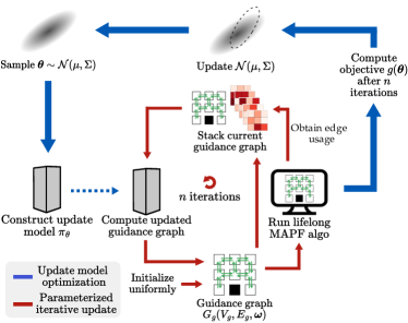
Figure 3: Parameterized Iterative Update (PIU): starting with initial edge weights uniformly, we iteratively run lifelong MAPF simulations to get the edge usage and wait action usage. We then use an update model $\pi_{\boldsymbol{\theta}}$ to update the edge weights. The update model $\pi_{\boldsymbol{\theta}}$ is optimized using CMA-ES.

Update Model Optimization. To train the update model, we define an objective function $g:\boldsymbol{\Theta}\rightarrow\mathbb{R}$ that runs the PIU algorithm for $N_{p}$ iterations with a given update model parameterized by vector $\boldsymbol{\theta}$. The throughput in the last iteration $f_{N_{p}}$ is returned as the output of $g$. We then search for optimal parameters $\boldsymbol{\theta^{*}}=\operatorname*{arg\,max}_{\boldsymbol{\theta}}g(\boldsymbol{\theta})$ using CMA-ES.

Algorithms 1, 1, 1, 1, 1, 1, 1, 1 and 1 of Algorithm 1 shows the pseudocode of update model optimization using CMA-ES. Starting with a given initial multi-variate Gaussian distribution (Algorithm 1), the algorithm iteratively samples $b$ parameter vectors (Algorithm 1) and runs PIU with them (Algorithms 1 and 1). Based on the returned throughput values, it keeps track of the best guidance graph (Algorithms 1 and 1) and updates the Gaussian distribution (Algorithm 1). Finally, the algorithm returns the best update model and the corresponding throughput (Algorithm 1).

Guidance Graph Generation with Update Model. To generate the guidance graph, we simply use the optimized update model to run PIU with a large $N_{e\_piu}=10$, meaning that the update model leverages traffic information from more lifelong MAPF simulations in each run to update the guidance graph. We further show the effect of the $N_{e\_piu}$ on the throughput of generated guidance graphs in Appendix C.

On the Advantage of PIU. Compared to directly using CMA-ES, the advantage of optimizing the update model and using PIU to generate guidance graph is two-folds. First, optimizing the update model reduces the dimension of search space. Although CMA-ES is versatile and applicable to various lifelong MAPF algorithms and maps, its effectiveness diminishes in high-dimensional search spaces, making it challenging to use CMA-ES to search for edge weights directly for large maps. Specifically, CMA-ES employs a full-rank $n\times n$ covariance matrix to model its Gaussian distribution in an $n$-dimensional space, leading to quadratic increases in both time and space complexity (Varelas et al., 2018). In the case of GGO, the number of edge weights of a guidance graph increases quadratically with the number of vertices, while our update model maintains a consistent number of parameters regardless of the size of the guidance graph, offering a more scalable solution than directly applying CMA-ES. Second, the optimized update model is not specific to the map it is optimized on. Different maps with similar layouts could potentially have similar high-throughput guidance graph that can be generated by the same update model. The guidance graph optimized by CMA-ES, on the other hand, consists of edge weights for a specific map.

5 Experimental Evaluation

In this section, we compare guidance graphs optimized by CMA-ES and PIU with various baselines and assess the capability of PIU to generate high-throughput guidance graphs for maps of larger sizes with similar layouts.

5.1 Experiment Setup

Setup	MAPF	Map	$N_{a}$	$N_{e\_cma}$	$N_{e\_piu}$	$N_{p}$	GGO
1	PIBT	random 32 $\times$ 32	400	5	1	5	CMA-ES & PIU
2		warehouse 33 $\times$ 36
3		room 64 $\times$ 64	1500
4	RHCR	warehouse 33 $\times$ 36	220	5	N/A	N/A	CMA-ES
5	DPP	warehouse 20 $\times$ 17	88	5	N/A	N/A	CMA-ES

Table 2: Summary of the experiment setup. $N_{a}$ is the number of agents, $N_{e\_cma}$ and $N_{e\_piu}$ are the number of lifelong MAPF simulations to run while evaluating each guidance graph in CMA-ES and PIU, respectively. $N_{p}$ is the number of iterations to run in PIU.

Setup	MAPF + GGO	SR	Throughput	CPU Runtime (s)
1	PIBT + CMA-ES	100%	$\textbf{7.78}\pm\textbf{0.02}$	$1.31\pm 0.01$
	PIBT + PIU	100%	$7.46\pm 0.02$	$1.29\pm 0.02$
	PIBT + Crisscross	100%	$6.84\pm 0.02$	$1.24\pm 0.02$
	PIBT + HM Cost	100%	$5.98\pm 0.02$	$1.17\pm 0.02$
	PIBT + Traffic Flow	100%	$7.43\pm 0.02$	$\textbf{1.19}\pm\textbf{0.02}$
	PIBT + Unweighted	100%	$5.52\pm 0.01$	$1.20\pm 0.02$
2	PIBT + CMA-ES	100%	$\textbf{7.64}\pm\textbf{0.01}$	$1.27\pm 0.01$
	PIBT + PIU	100%	$7.28\pm 0.01$	$1.22\pm 0.01$
	PIBT + Crisscross	100%	$6.65\pm 0.01$	$\textbf{1.21}\pm\textbf{0.01}$
	PIBT + HM Cost	100%	$5.63\pm 0.01$	$1.24\pm 0.01$
	PIBT + Traffic Flow	100%	$5.84\pm 0.01$	$1.23\pm 0.01$
	PIBT + Unweighted	100%	$5.22\pm 0.01$	$1.25\pm 0.01$
3	PIBT + CMA-ES	100%	$3.12\pm 0.01$	$4.91\pm 0.06$
	PIBT + PIU	100%	$\textbf{3.13}\pm\textbf{0.01}$	$4.59\pm 0.05$
	PIBT + Crisscross	100%	$2.75\pm 0.01$	$4.67\pm 0.07$
	PIBT + HM Cost	100%	$2.41\pm 0.01$	$4.71\pm 0.05$
	PIBT + Traffic Flow	100%	$2.87\pm 0.01$	$\textbf{4.55}\pm\textbf{0.05}$
	PIBT + Unweighted	100%	$2.51\pm 0.01$	$4.95\pm 0.06$
4	RHCR + CMA-ES	100%	$\textbf{6.58}\pm\textbf{0.04}$	$\textbf{91.24}\pm\textbf{15.66}$
	RHCR + Crisscross	100%	$5.59\pm 0.20$	$3771.71\pm 659.20$
	RHCR + HM Cost	$0\%$	N/A	N/A
	RHCR + Traffic Flow	$32\%$	$3.57\pm 0.20$	$324.12\pm 63.91$
	RHCR + Unweighted	$0\%$	N/A	N/A
5	DPP + CMA-ES	100%	$\textbf{5.17}\pm\textbf{0.00}$	$28.75\pm 0.53$
	DPP + Crisscross	100%	$4.76\pm 0.01$	$\textbf{17.36}\pm\textbf{0.31}$
	DPP + HM Cost	100%	$4.32\pm 0.01$	$29.94\pm 1.39$
	DPP + Traffic Flow	100%	$4.07\pm 0.00$	$578.43\pm 53.61$
	DPP + Unweighted	100%	$4.34\pm 0.01$	$20.30\pm 0.49$

Table 3: Success rates, throughput, and CPU runtimes of the guidance graphs. SR refers to the success rate. For RHCR and DPP, the success rate is the percentage of simulations that end without congestion. For PIBT, it is the percentage of simulations that end without timeout. CPU runtime refers to the runtime of the simulation in seconds. We only measure the throughput and CPU runtime of successful simulations.

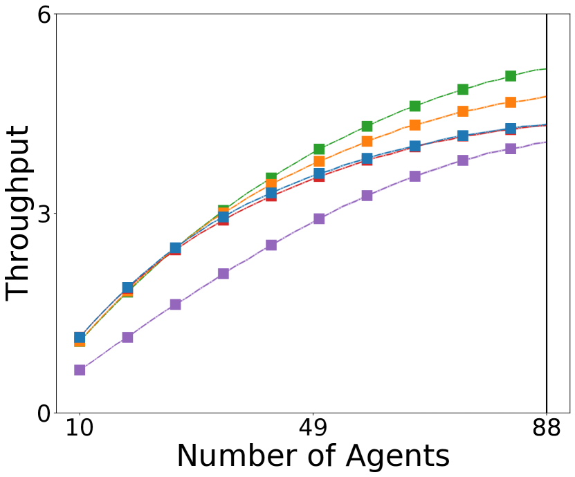
(a) warehouse 20 $\times$ 17

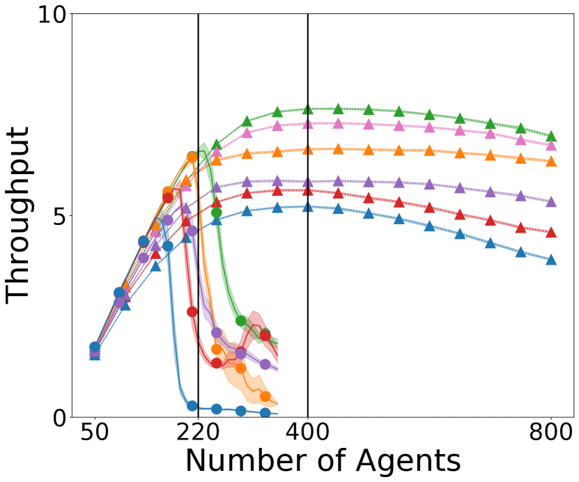
(b) warehouse 33 $\times$ 36

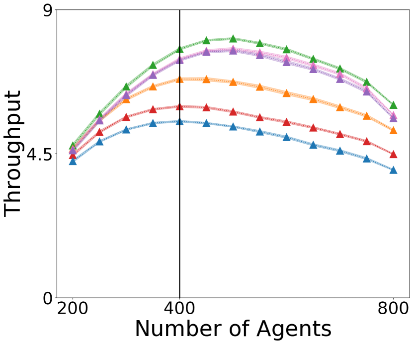
(c) random 32 $\times$ 32

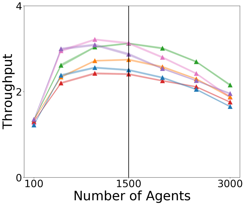
(d) room 64 $\times$ 64

Figure 4: Throughput with different numbers of agents. The guidance graphs are optimized with $N_{a}$ agents, which is indicated by the black vertical lines. In (b), the black vertical lines at 220 and 400 agents indicate $N_{a}$ for setups 4 and 2, respectively.

General Setups. Table 2 outlines our experimental setup. Column 2 shows the lifelong MAPF algorithms. Following the recommendations of previous works (Li et al., 2021; Zhang et al., 2023b), we use PBS (Ma et al., 2019) and SIPP (Phillips and Likhachev, 2011) as the MAPF solver and the single-agent solver, respectively, in both RHCR and DPP and use $h=5$ and $w=10$ in RHCR. Column 3 outlines the maps, all being 4-neighbor girds, including two warehouse maps (warehouse 33 $\times$ 36 and warehouse 20 $\times$ 17) from previous works (Li et al., 2021; Zhang et al., 2023b) and two additional maps (random 32 $\times$ 32 and room 64 $\times$ 64) from the MAPF benchmark (Stern et al., 2019); see Figure 8 in Appendix B for illustration. We choose multiple maps for PIBT to demonstrate that both CMA-ES and PIU work for different maps. Column 4 is the number of agents used in lifelong MAPF simulations, with a larger $N_{a}$ for PIBT compared to RHCR and DPP to demonstrate that both CMA-ES and PIU work for congested scenarios.

Columns 5 to 7 show the hyerparameters of CMA-ES and PIU. To ensure a fair comparison, we choose the hyperparameters such that CMA-ES and PIU run the same number of lifelong MAPF simulations. In particular, we set batch size $b=100$ and the number of iterations $I=100$ for both CMA-ES and PIU, resulting in a total of $b\times I=10$k objective function evaluations for both algorithms. In each iteration, we select the top $N_{best}=50$ solutions to update the Gaussian distribution. For CMA-ES, each evaluation runs $N_{e\_cma}=5$ lifelong MAPF simulations, resulting in $50$k simulations. For PIU, each evaluation runs the PIU algorithm for $N_{p}$ iterations and each iteration runs $N_{e\_piu}=1$ simulation, resulting in $50$k simulations, identical to CMA-ES. We run each simulation for 1,000 timesteps. For RHCR and DPP, we stop the simulation early in case of congestion, which happens if more than half of the agents wait at their current location.

Column 8 shows the GGO algorithms we run for each setup. We apply CMA-ES across all setups to demonstrate its versatility. However, due to computational constraints, we focus on using PIU primarily with PIBT. While both PIU and CMA-ES conduct the same number of lifelong MAPF simulations, there is a notable difference in their execution. In CMA-ES, all $N_{e\_cma}$ simulations in each guidance graph evaluation can be parallelized. In contrast, PIU runs the simulations sequentially, resulting in slower runtime.

Update Model. To enable the update model to generate guidance graphs for arbitrary maps, we use a Convolutional Neural Network (CNN) as our update model. We can use CNN because we choose grid-based maps in the experiments. The CNN has 3 convolutional layers of kernel size 3 $\times$ 3, each followed by a ReLU activation. The update model has 4,231 parameters. For a map of dimension $h\times w$, we represent the edge weights $\boldsymbol{\omega}$ of the guidance graph as a tensor of size $h\times w\times 5$, where the first four channels are the movement costs and the last channel is the wait costs.

Baseline Guidance. As mentioned in Section 3, we have 4 baseline guidance graphs, namely (1) Unweighted, (2) Crisscross (Cohen, 2020), (3) HM Cost (Cohen et al., 2016b), and (4) Traffic Flow (Chen et al., 2024).

Transfer Optimized Updated Model. We attempt to transfer the update model optimized with setup 2 to larger warehouse maps with similar layouts. Specifically, we mimic the layout of warehouse 33 $\times$ 36 in setup 2 and design larger warehouse maps with sizes up to 93 $\times$ 91. We show the larger maps and other experiment setups including implementation and computation resources in Appendix B.

5.2 Results

5.2.1 Comparing GGO with Baseline Guidance

We first compare our optimized guidance graph with the baseline guidance graphs. For each guidance graph, we run 50 simulations and report the numerical results in Table 3 in the format of $x\pm y$, where $x$ is the average and $y$ is the standard error. Both CMA-ES and PIU outperform all baseline guidance graphs in all setups in terms of throughput. Specifically, CMA-ES outperforms all baseline guidance graphs in all setups, showing the versatility of the algorithm. For the baseline methods, the human-designed crisscross guidance performs quite well in setups 2, 4, and 5 in warehouse 33 $\times$ 36 and warehouse 20 $\times$ 17 while Traffic Flow is more competitive in setups 1 and 3 with random 32 $\times$ 32 and room 64 $\times$ 64.

When comparing CMA-ES and PIU, CMA-ES outperforms PIU in setups with smaller maps (warehouse 20 $\times$ 17, warehouse 33 $\times$ 36, and random 32 $\times$ 32), but matches PIU in the larger room 64 $\times$ 64 map because CMA-ES scales poorly to high-dimensional search space. The guidance graph of room 64 $\times$ 64 has 14,340 parameters, making the optimization very challenging. Optimizing the update model with PIU, on the other hand, has a lower-dimensional search space of 4,231 parameters regardless of map size, making PIU advantageous in large maps.

(a) random 32 $\times$ 32

(b) warehouse 33 $\times$ 36

Figure 5: Edge weights of the outgoing edges of Traffic Flow guidance graphs at every vertex in warehouse 33 $\times$ 36 and random 32 $\times$ 32 maps.

To further understand the performance of the optimized guidance graphs, we run lifelong MAPF simulation with various numbers of agents and plot the throughput in Figure 4. The trends are similar in all maps, with CMA-ES and PIU generally outperforming all baselines, except that Traffic Flow matches PIU with fewer agents In random 32 $\times$ 32 and room 64 $\times$ 64. However, Traffic Flow is less competitive in warehouse 33 $\times$ 36 and warehouse 20 $\times$ 17, indicating that the performance of Traffic Flow depends on the map structure. To illustrate such dependency, we show the edge weights of the guidance graph as heatmaps in Figure 5. It is notable that the edge weights in the center of the random 32 $\times$ 32 map are higher, promoting the agents to traverse the edges on the peripheral area. In the warehouse 33 $\times$ 36 map, however, the vertical lanes of empty spaces (white tiles shown in Figure 8(b)) are heavily congested, inflating the edge weights in those vertices almost equally. Therefore, the guidance given by the graph in Figure 5(b) is less informative than that in Figure 5(a), causing Traffic Flow to have inferior performance in the warehouse 33 $\times$ 36 map.

5.2.2 PIBT and RHCR with GGO

Setup	MAPF	Map	$N_{a}$	$N_{e\_cma}$	$N_{e\_piu}$	$N_{p}$	GGO
6	PIBT	warehouse 33 $\times$ 36	150	5	1	5	CMA-ES/PIU

Table 4: An additional the experiment setup to compare PIBT with RHCR when there are fewer agents.

Setup	MAPF + GGO	SR	Throughput	CPU Runtime (s)
6	PIBT + CMA-ES	100%	$4.74\pm 0.01$	$0.58\pm 0.00$
	PIBT + PIU	100%	$4.77\pm 0.01$	$0.58\pm 0.01$
	PIBT + Unweighted	100%	$3.75\pm 0.00$	$\textbf{0.50}\pm\textbf{0.00}$
	RHCR + Unweighted	100%	$\textbf{4.95}\pm\textbf{0.00}$	$87.37\pm 0.72$

Table 5: Success rates, throughput, and CPU runtimes of the guidance graphs comparing RHCR and PIBT with the same number of agents in setup 6.

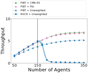
Figure 6: A well-optimized guidance graph enables PIBT to have competitive throughput with RHCR despite the advantage of RHCR with fewer agents.

In Figure 4, we additionally observe improved throughput for PIBT in warehouse 33 $\times$ 36 with fewer agents. To illustrate how a well-optimized guidance graph can narrow the throughput gap between RHCR and PIBT, we conduct additional experiments as detailed in Table 4. We choose $N_{a}=150$ because it is the largest number with which RHCR can maintain 100% success rate using an unweighted guidance graph.

Table 5 shows the numerical results comparing RHCR with an unweighted guidance graph and PIBT with optimized guidance graphs. We run 50 simulations, each with 1000 timesteps, and report the average and standard errors. We find that, while RHCR still has the highest throughput, both GGO methods significantly reduce the throughput gap between PIBT and RHCR, from 24.2% to less than 4.2%, This indicates that, with the help of our optimized guidance graph, we can enable a greedy, distributed, yet extremely fast rule-based MAPF algorithm (PIBT) to achieve performance comparable to a centralized, computationally heavy, search-based MAPF algorithm (RHCR). Figure 6 further compares PIBT and RHCR with various numbers of agents. We observe that the throughput of RHCR quickly drops after 150 agents, while PIBT can maintain an increasing trend with more agents.

5.2.3 Transfer Optimized Update Model

Figure 7: Max throughput and the number of agents at this maximum. PIU Transfer refers to using the update model optimized in setup 2 to generate guidance graphs.

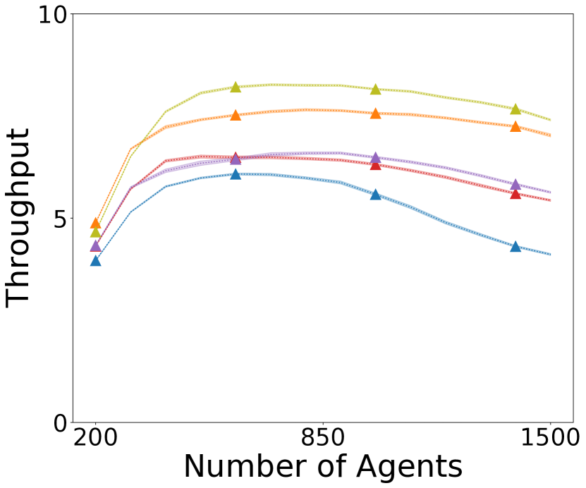
(a) 45 $\times$ 47

(b) 57 $\times$ 58

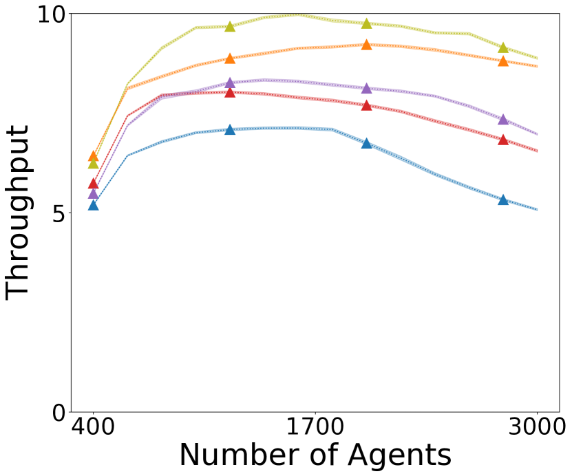
(c) 69 $\times$ 69

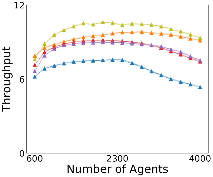
(d) 81 $\times$ 80

(e) 93 $\times$ 91

Figure 10: Throughput with different numbers of agents in larger warehouse maps.

We use the update model optimized in setup 2 to test transferability. We first use the optimized update model to generate guidance graphs for maps with different sizes but similar layouts (specified in Figure 9 of Appendix B) with an increasing number of agents, ranging from around 10% to 90% of the non-obstacles in the maps. We then run 50 lifelong MAPF simulations in each of the generated guidance graphs with PIBT. We plot the maximum throughput achieved in each map and the corresponding number of agents in Figure 7, comparing PIU Transfer with baseline guidance graphs. We observe that PIU Transfer dominates all baselines with all sizes. We further show the throughput with different numbers of agents in each map in Figure 10 of Appendix C.

6 Conclusion

We define guidance graph and GGO to maximize the throughput of lifelong MAPF, reviewing previous works on guidance in MAPF and highlighting the generality of our guidance graph. We propose two GGO approaches, CMA-ES and PIU, that optimize guidance graph across different algorithms and maps. We also show the ability of update model to generate guidance graph for larger maps with similar patterns.

Our work is limited in many ways, yielding numerous future directions. First, both CMA-ES and PIU are computationally expensive, requiring a large number of lifelong MAPF simulations. Future works can focus on reducing the computational requirements of both methods. Second, although our guidance graph can be used with online update mechanisms introduced in previous works (Chen et al., 2024; Yu and Wolf, 2023), we limit our experiment settings without such mechanisms. Integrating these mechanisms with our GGO approach could further enhance MAPF guidance utility.

Appendix A Baseline Guidance Graphs

In this section, we discuss the baseline guidance graphs that we compare with in Section 5. As mentioned in Section 3, we have 4 baseline guidance graphs, namely (1) Unweighted, (2) Crisscross [Cohen, 2020], (3) HM Cost [Cohen et al., 2016a], and (4) Traffic Flow [Chen et al., 2024].

1

Input: $G_{g}(V_{g},E_{g},\boldsymbol{\omega})$, where $\boldsymbol{\omega}=1$
$N_{base}$: number of iterations
$S,T\subset V_{g}$: potential start and goal locations of the agents
$plan\_path$: function to find single agent path given start, goal, and guidance graph.

2

3Initialize vertex usage $U_{V_{g}}(v)\leftarrow 0,\forall v\in V_{g}$

4 Initialize edge usage $U_{E_{g}}(u,v)\leftarrow 0,\forall(u\rightarrow v)\in E_{g}$

5 for $i\leftarrow 1$ to $N_{base}$ do

6       Sample $s_{i}\in_{R}S,g_{i}\in_{R}T$ s.t. $s_{i}\neq g_{i}$

7       $P_{i}\leftarrow plan\_path(s_{i},g_{i},G_{g})$

8       for Vertex $v\in P_{i}$ do

9             $U_{V_{g}}(v)\leftarrow U_{V_{g}}(v)+1$

10            

11      for Edge $(u\rightarrow v)\in P_{i}$ do

12             $U_{E_{g}}(u,v)\leftarrow U_{E_{g}}(u,v)+1$

13            

14      for Edge $(u\rightarrow v)\in E_{g}$ do

15             $p(v)\leftarrow\lceil\frac{U_{V_{g}}(v)-1}{2}\rceil$

16             $c(u,v)\leftarrow U_{V_{g}}(u,v)\times U_{V_{g}}(v,u)$

17             $\boldsymbol{\omega}(u,v)\leftarrow 1+c(u,v)+p(v)$

18            

19      

20$\boldsymbol{\omega}_{TF}\leftarrow\boldsymbol{\omega}$

21 Return $G_{TF}(V_{g},E_{g},\boldsymbol{\omega}_{TF})$

Algorithm 2 Traffic Flow Guidance Graph Generation

A.1 Unweighted and Crisscross

Both unweighted and crisscross guidance graphs are human-designed. We define unweighted guidance graph as follows:

Definition 6 (Unweighted Guidance Graph).

We define a guidance graph $G(V_{g},E_{g},\boldsymbol{\omega})$ where $\boldsymbol{\omega}=1$ as an unweighted guidance graph.

Our crisscross guidance graph follows the definition of crisscross highways [Cohen, 2020]. In particular:

Definition 7 (Crisscross Guidance Graph).

Given an unweighted guidance graph $G(V_{g},E_{g},\boldsymbol{\omega})$ for a 4-neighbor grid-based map in which agents can move up, down, left, or right at each vertex, we select a subset of edges $E_{c}\subset E_{g}$ such that:

1. in the even rows, all edges pointing right are chosen,

2. in the odd rows, all edges pointing left are chosen,

3. in the even columns, all edges pointing up are chosen,

4. in the odd columns, all edges pointing down are chosen.

We let the edge weights of edges in $E_{c}$ be 0.5 and all other edges $E_{g}\setminus E_{c}$ be 1, promoting the agents to use edges in $E_{c}$.

A.2 Traffic Flow and HM Cost

1

Input: $G_{g}(V_{g},E_{g},\boldsymbol{\omega})$, where $\boldsymbol{\omega}=1$
$N_{base}$: number of iterations
$S,T\subset V_{g}$: potential start and goal locations of the agents
$plan\_path$: function to find single agent path given start, goal, and guidance graph.
$\alpha,\beta,\gamma\in\mathbb{R}$: hyperparameters of computing follow preference $p$, interference cost $t$, and saturation cost $t$, respectively.

2

3Initialize vertex usage $U_{V_{g}}(v)\leftarrow 0,\forall v\in V_{g}$

4 Initialize edge usage $U_{E_{g}}(u,v)\leftarrow 0,\forall(u\rightarrow v)\in E_{g}$

5 for $i\leftarrow 1$ to $N_{base}$ do

6       Sample $s_{i}\in_{R}S,g_{i}\in_{R}T$ s.t. $s_{i}\neq g_{i}$

7       $P_{i}\leftarrow plan\_path(s_{i},g_{i},G_{g})$

8       for Vertex $v\in P_{i}$ do

9             $U_{V_{g}}(v)\leftarrow U_{V_{g}}(v)+1$

10            

11      for Edge $(u\rightarrow v)\in P_{i}$ do

12             $U_{E_{g}}(u,v)\leftarrow U_{E_{g}}(u,v)+1$

13            

14      for Edge $(u\rightarrow v)\in E_{g}$ do

15             $p(u,v)\leftarrow\alpha\times\frac{U_{E_{g}}(u,v)}{N_{base}}$

16             $t(u,v)\leftarrow\beta\times\frac{U_{E_{g}}(v,u)}{N_{base}}$

17             $s(u,v)\leftarrow\gamma^{\frac{U_{E_{g}}(u,v)+U_{E_{g}}(v,u)}{2N_{base}}}$

18             $c(u,v)\leftarrow 1-p(u,v)+t(u,v)+s(u,v)$

19             $\boldsymbol{\omega}(u,v)\leftarrow c(u,v)$

20            

21      

22

23Set $E_{HM}\subset E_{g}$ with lowest $c(u,v)$ s.t. $|E_{HM}|=\frac{1}{7}|E_{g}|$ and $u\neq v$

24 Set $E_{HM}^{\prime}\leftarrow$ randomly sample $\frac{1}{5}$ of edges from $E_{HM}$

25 Initialize edge weights $\boldsymbol{\omega}_{HM}$

26 for Edge $(u\rightarrow v)\in E_{g}$ do

27       if $(u\rightarrow v)\in E_{HM}^{\prime}$ then

28             $\boldsymbol{\omega}_{HM}(u,v)\leftarrow 0.5$

29            

30      else

31             $\boldsymbol{\omega}_{HM}(u,v)\leftarrow 1$

32            

33      

34Return $G_{HM}(V_{g},E_{g},\boldsymbol{\omega}_{HM})$

Algorithm 3 HM Cost Guidance Graph Generation

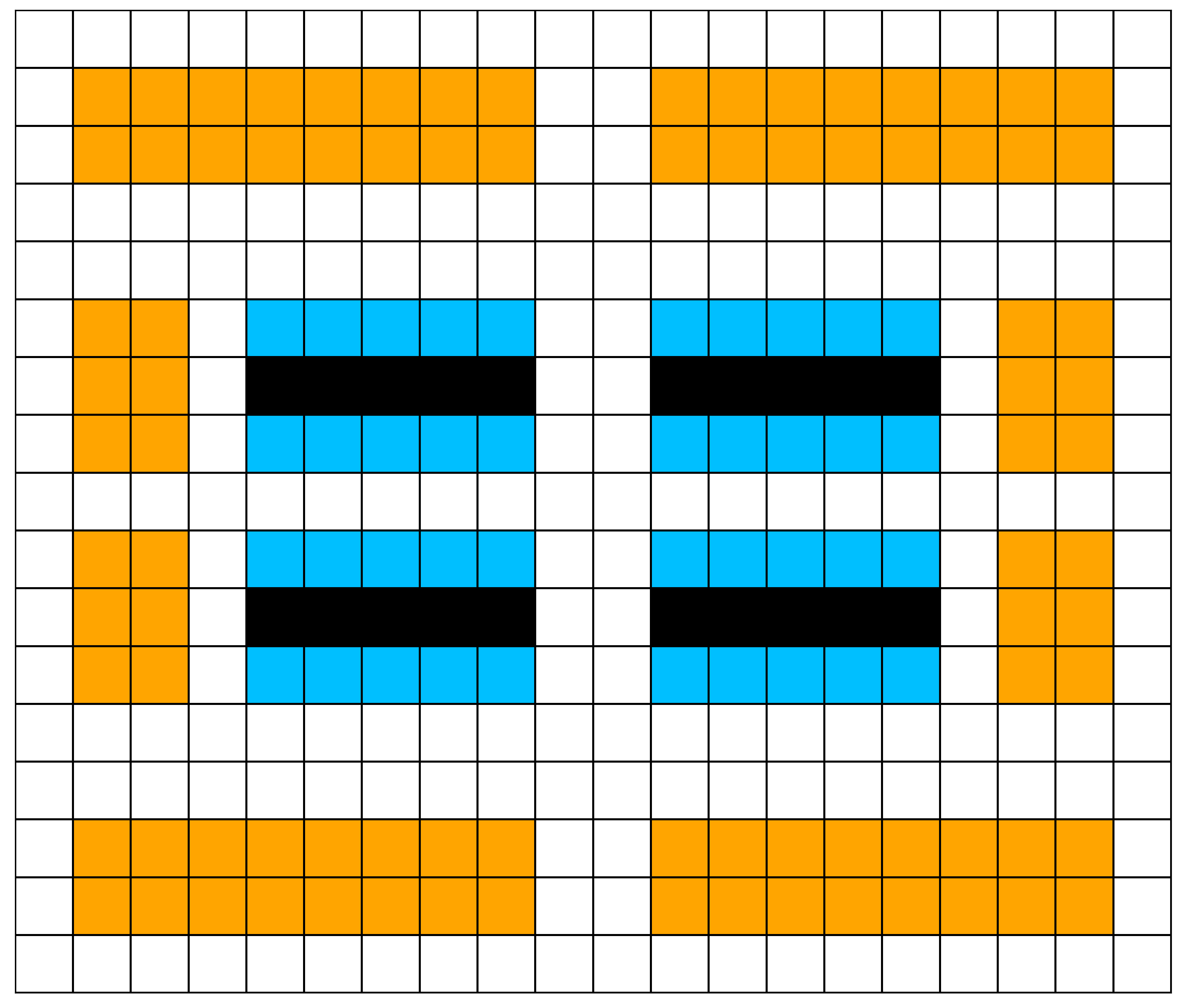
(a) warehouse 20 $\times$ 17

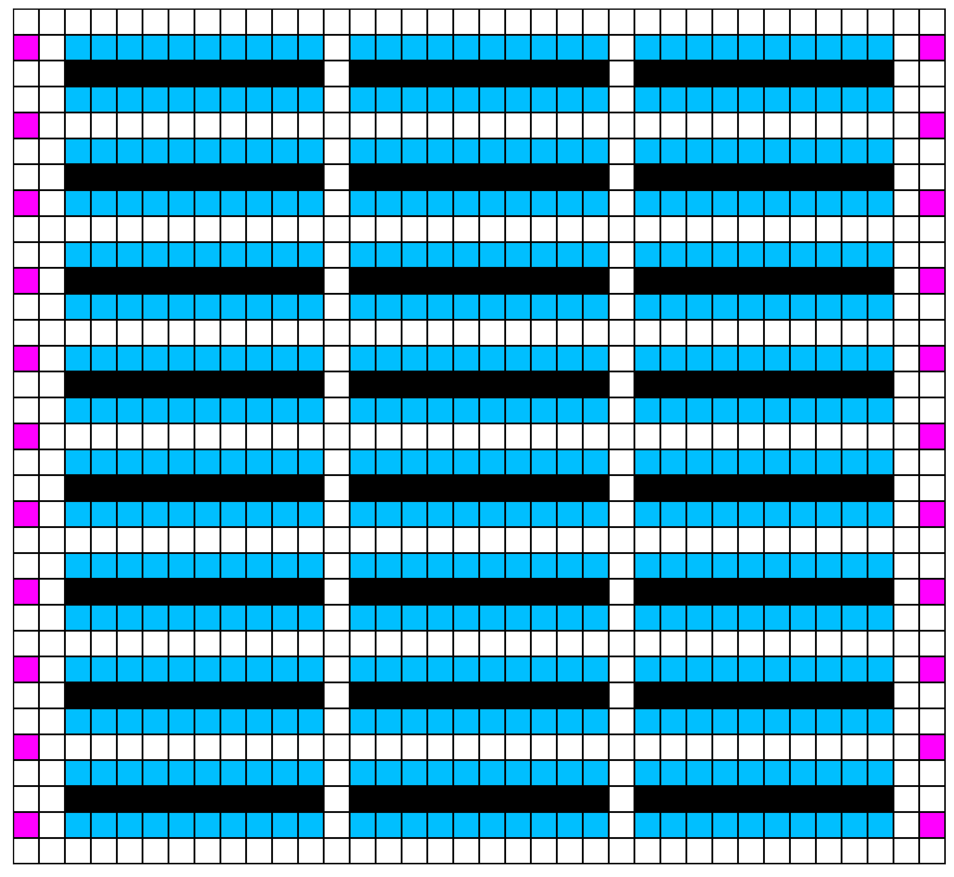
(b) warehouse 33 $\times$ 36

(c) random 32 $\times$ 32

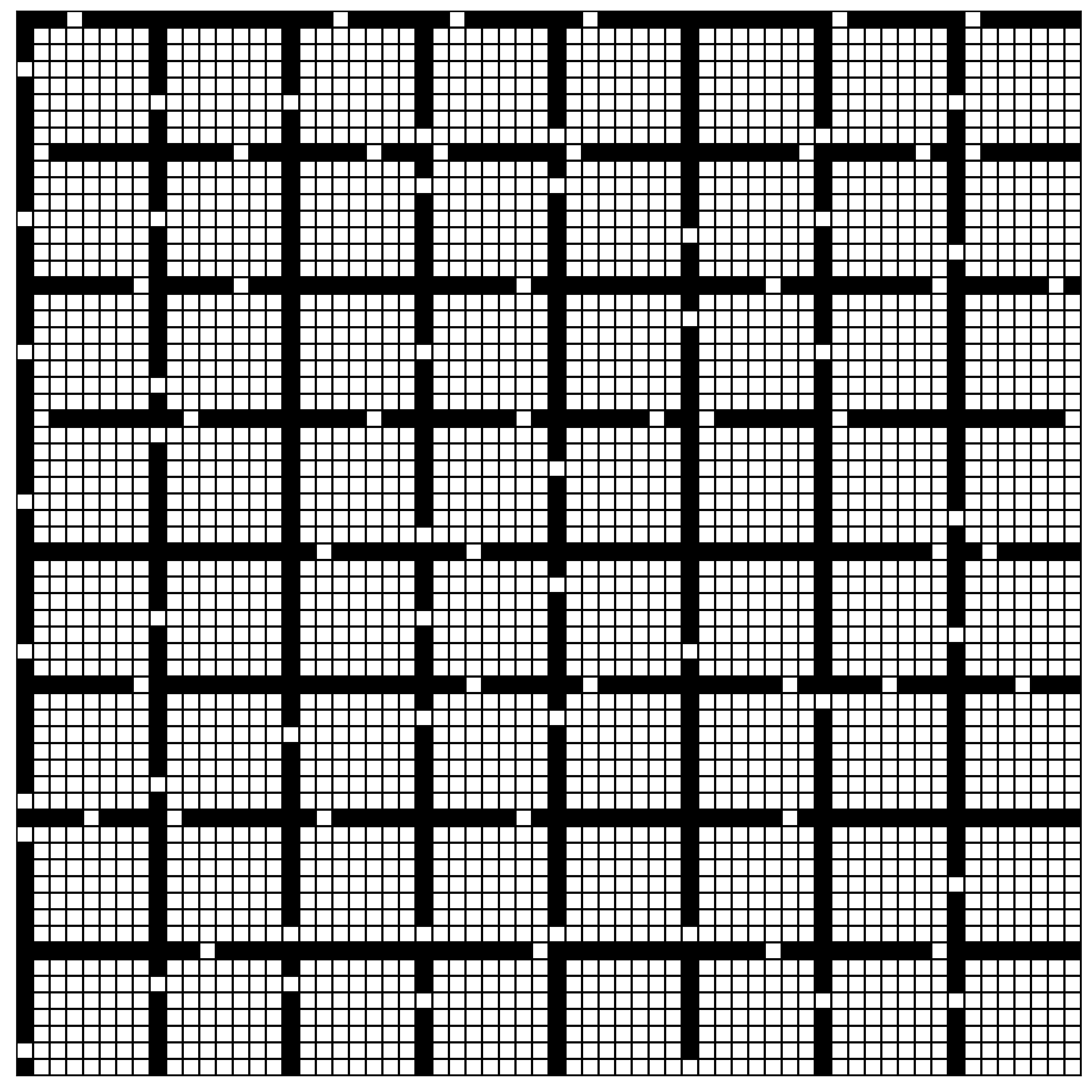
(d) room 64 $\times$ 64

Figure 8: Maps used for experiments.

The previous work on traffic flow guidance [Chen et al., 2024] is developed for lifelong MAPF with an online update mechanism. The work on HM Cost guidance [Cohen et al., 2016b] is developed for one-shot MAPF. Therefore, we adapt both methods to construct guidance graphs for lifelong MAPF.

Traffic Flow. Algorithm 2 describes the adapted Traffic Flow guidance graph generation procedure. On a high level, we iteratively plan single-agent paths based on the current guidance graph and update the graph based on the congestion of these paths. Starting with an unweighted guidance graph, we sample a pair of start and goal locations (Algorithm 2) and search for a path $P_{i}$ that minimizes the sum of its edge weights on the current guidance graph (Algorithm 2). Then, we increment the usages of vertices and edges on $P_{i}$ by 1 (Algorithms 2, 2, 2 and 2). Afterward, we follow the previous work [Chen et al., 2024] to compute the vertex congestion averaged over vertex usage for each vertex (Algorithm 2) and the contraflow congestion for each edge (Algorithm 2) and then update the edge weights of the guidance graph by summing the vertex congestion, the contraflow congestion, and 1 (Algorithm 2), where the 1 indicates the zero congestion cost. The updated edge weights inflate the cost of frequently used edges so that the following single-agent paths are encouraged to avoid these edges. Traffic Flow repeats the procedure for $N_{base}$ iterations and returns the edge weights from the last iteration as the guidance graph (Algorithms 2 and 2). Since the Traffic Flow algorithm does not consider wait costs, we set wait costs of all vertices to be 1.

HM Cost. Algorithm 3 describes the adapted HM Cost guidance graph generation procedure. Similar to Traffic Flow, we first sample start and goal locations (Algorithm 3) and run single-agent path planning on the current guidance graph (Algorithm 3), updating vertex and edge usage (Algorithms 3, 3, 3 and 3). Then we follow the previous work [Cohen et al., 2016b] to compute (1) the follow preference $p$ (Algorithm 3), which encourages the agents to traverse through previously used edges, (2) the interference cost $t$, which discourages the agents to traverse through edges in the opposite directions of previously used edges, and (3) the saturation cost $s$. The HM cost $c$ is a linear combination of the above three variables (Algorithm 3), with smaller HM costs indicating edges that are used more frequently. We then set the HM cost as the edge weights of the guidance graph and repeat the iteration for $N_{base}$ times (Algorithm 3).

Nevertheless, after running $N_{base}$ single agent path planning, HM Cost includes additional procedures to generate the final guidance graph from the computed HM cost. Following previous work [Cohen et al., 2016b], we select the top $\frac{1}{7}$ of the edges with the smallest HM cost and then randomly sample $\frac{1}{5}$ of them as the set of highway edges (Algorithms 3 and 3). We then set the weights of the highway edges as 0.5 and non-highway edges as 1, forming a guidance graph (Algorithms 3, 3, 3, 3, 3 and 3). In HM Cost, all selected edges are not self-edges. Therefore, the wait costs of all vertices are 1, same as the non-highway edges.

Appendix B Additional Experiment Setups

B.1 Maps

Figure 8 summarizes the maps used for experiments in Section 5. In all maps, black tiles are obstacles and non-black tiles are traversable. In warehouse maps, orange tiles are home-locations, blue tiles are endpoints, and purple tiles are workstations. In warehouse 20 $\times$ 17, agents start from orange tiles (home-locations) and move constantly between randomly chosen blue tiles. In warehouse 33 $\times$ 36, agents start from any non-black tiles and move between randomly chosen blue and purple tiles. In random 32 $\times$ 32 and room 64 $\times$ 64, agents start from and move between randomly chosen white tiles.

Figure 9 summarizes the warehouse maps used to test transferability of the optimized update model in Section 5. To create these maps, we mimic the pattern of Figure 8(b), repeating block of 10 shelves (black) and endpoints (blue) and placing workstations (purple) on the left and right borders.

B.2 Hyperparameters for Baseline Methods

In both Traffic Flow and HM Cost, we use $N_{base}=10,000$ to generate the guidance graphs for all maps. In HM Cost, we follow the previous work [Cohen et al., 2016b] to use $\alpha=0.5$, $\beta=1.2$, and $\gamma=1.3$.

B.3 Implementation.

We implement CMA-ES in Pyribs [Tjanaka et al., 2023] and the update model in PyTorch [Paszke et al., 2019]. We have included the source in the supplementary material. We implement Traffic Flow and HM Cost guidance graph generation in Python. We implement the lifelong MAPF algorithms in C++ based on openly available implementation from the previous works [Li et al., 2021; Okumura et al., 2019].

B.4 Compute Resource

We run our experiments on two machines: (1) a local machine with a 64-core AMD Ryzen Threadripper 3990X CPU, 192 GB of RAM, and an Nvidia RTX 3090Ti GPU, and (2) a high-performing cluster with numerous 64-core AMD EPYC 7742 CPUs, each with 256 GB of RAM. We measure all CPU runtime on machine (1).

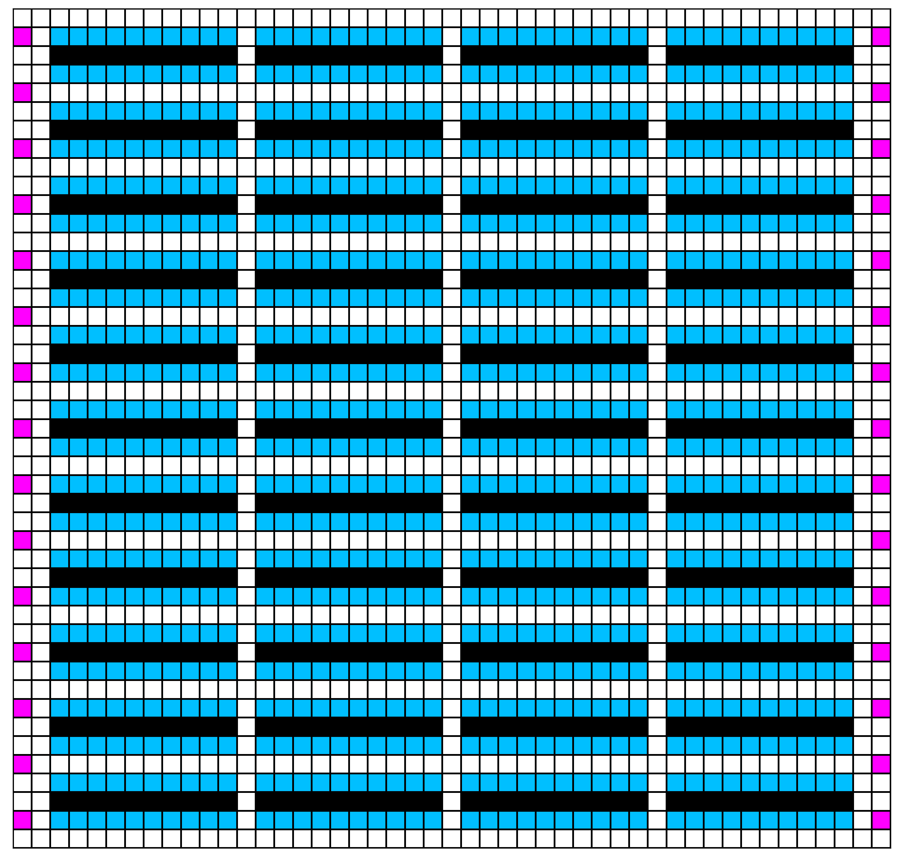
(a) 45 $\times$ 47

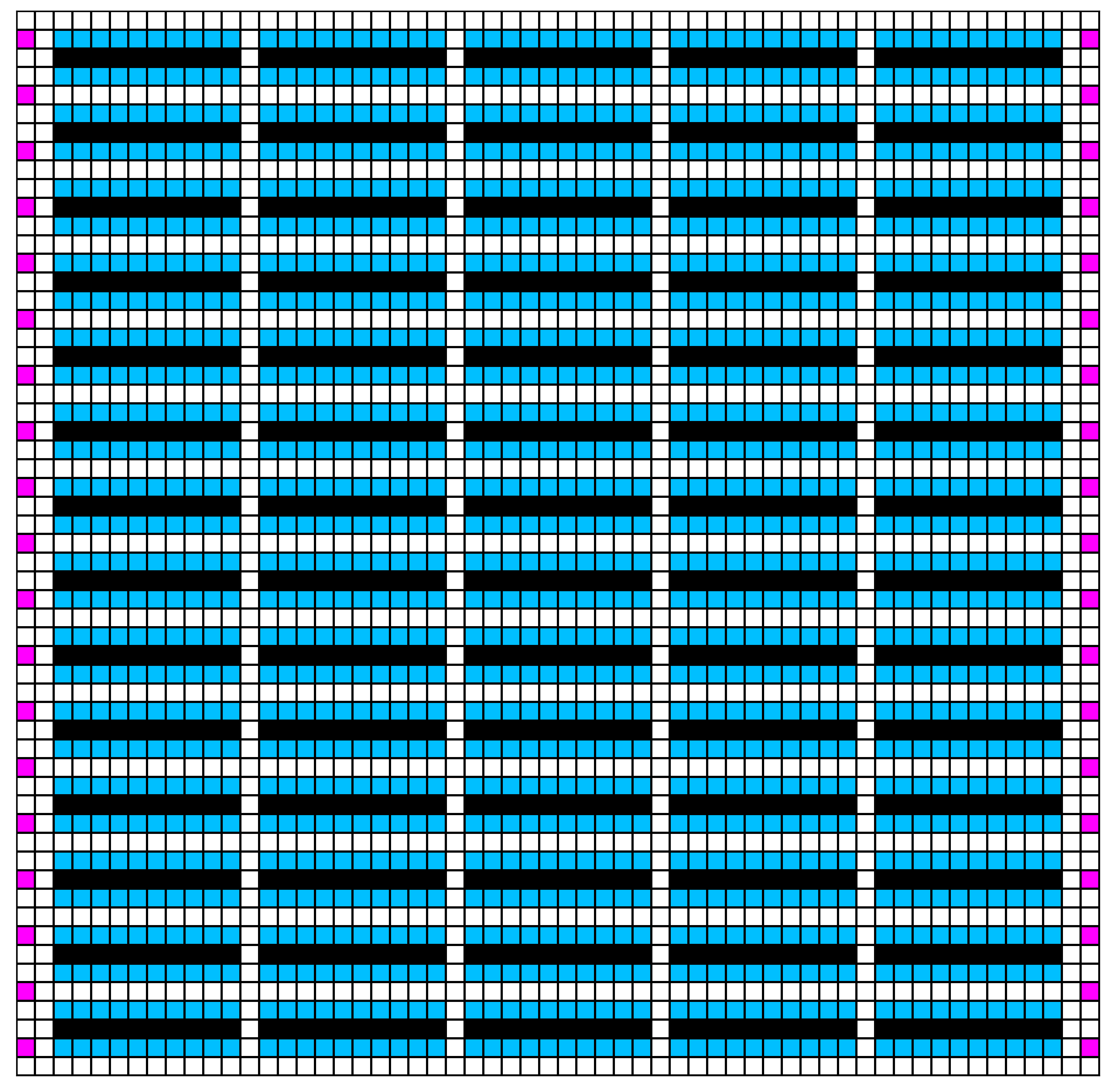
(b) 57 $\times$ 58

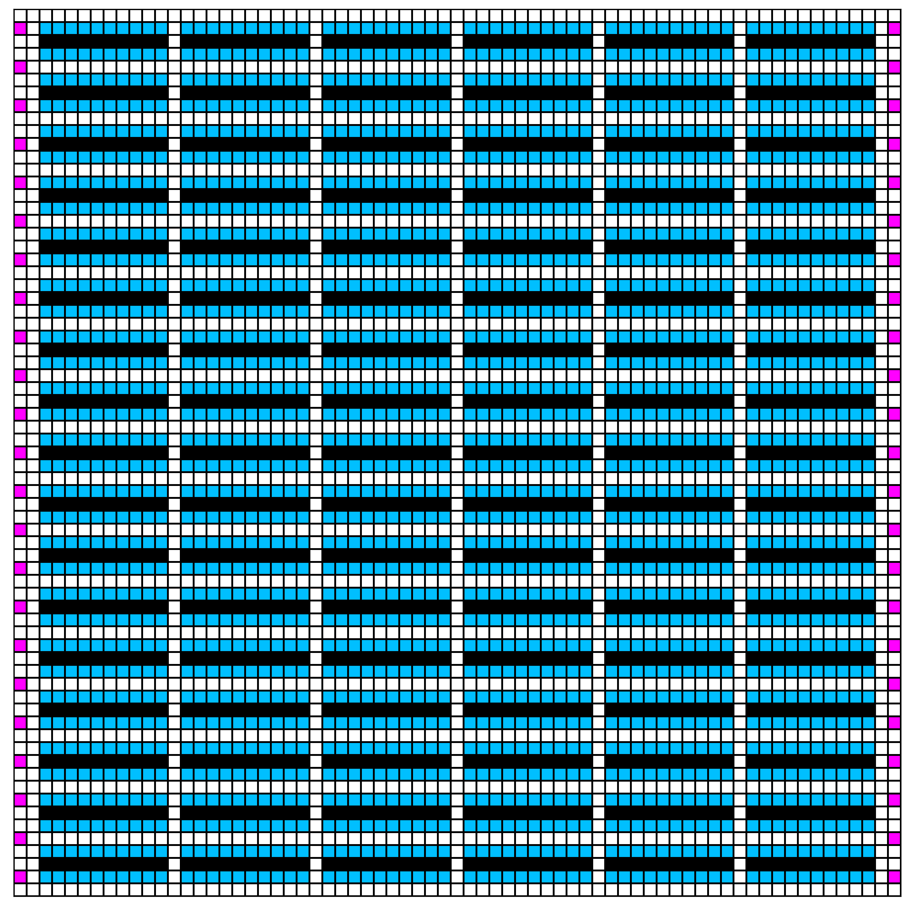
(c) 69 $\times$ 69

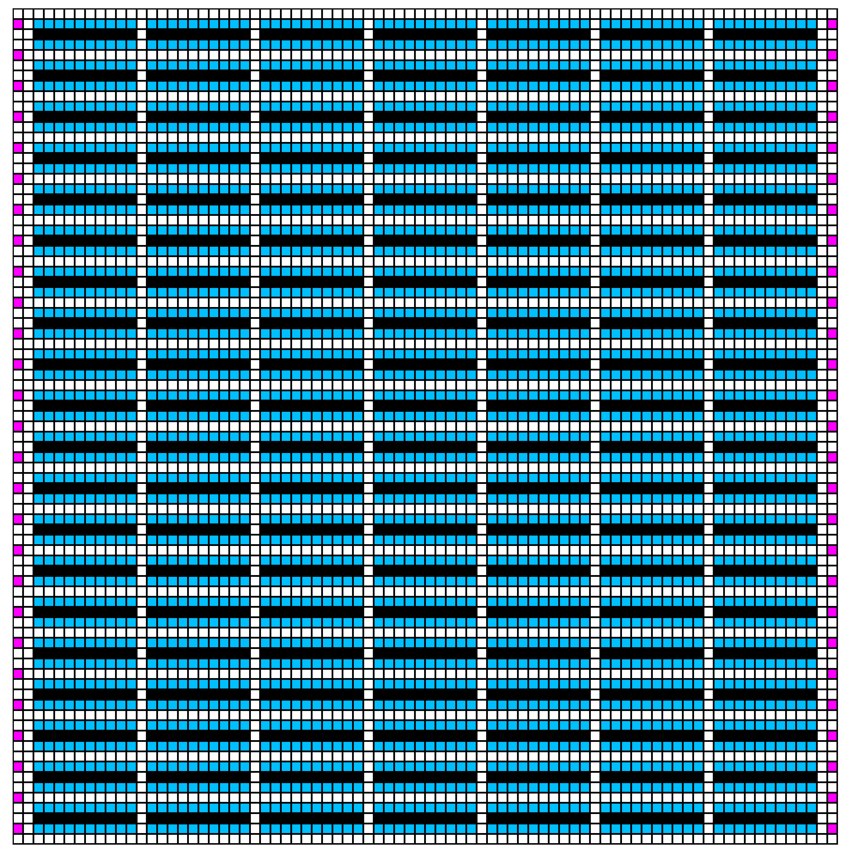
(d) 81 $\times$ 80

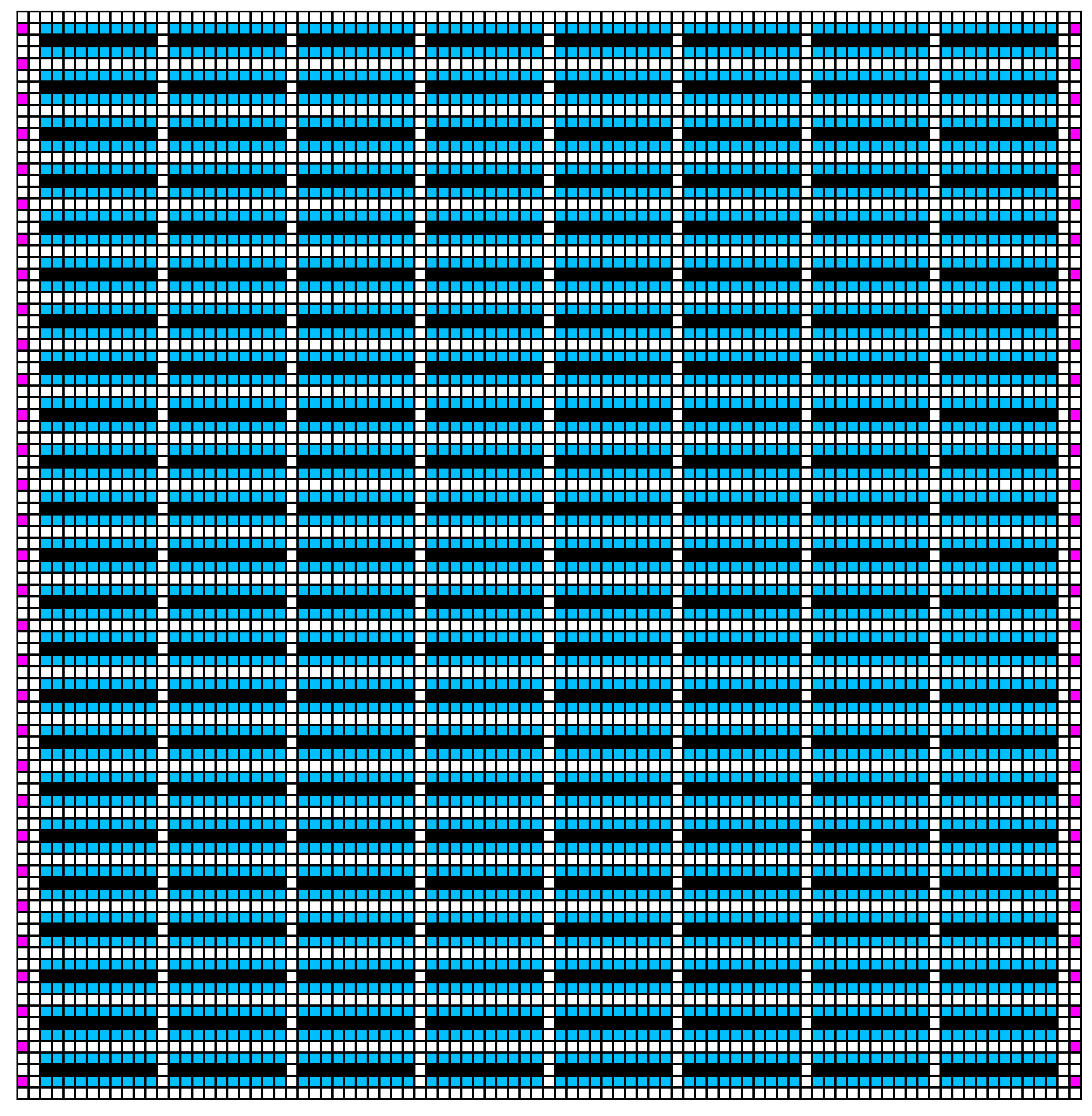
(e) 93 $\times$ 91

Figure 9: Warehouse maps used for testing the transferability of the update model optimized with setup 2 in Section 5.

Appendix C Additional Experiments

We include the following additional experiments: (1) for PIU, we test guidance graph generation with different values of $N_{e\_piu}$ to test if running more simulations in PIU can improve the generated guidance graph, and (2) for bounds handling of CMA-ES, we show ablation experiments on normalization comparing with other representative bounds handling methods presented in [Biedrzycki, 2020].

C.1 On the Value of $N_{e\_piu}$

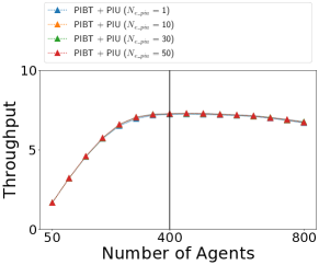
Figure 11: Effect of different values of $N_{e\_piu}$. The black vertical line indicates the number of agents used to optimize the update model.

We use the update model optimized with setup 2 to generate guidance graphs with $N_{e\_piu}\in\{1,10,30,50\}$. We then evaluate the guidance graphs by running lifelong MAPF simulations with various number of agents, each with 50 simulations. We show the result in Figure 11. We find no significant difference in throughput with different values of $N_{e\_piu}$.

C.2 Bounds Handling in CMA-ES

(a) Setup 1: random 32 $\times$ 32

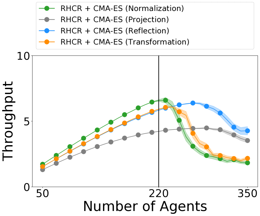
(b) Setup 4: warehouse 33 $\times$ 36

Figure 12: Comparison of different bounds handling methods in CMA-ES in setup 1 and 4. The black vertical lines indicates the number of agents $N_{a}$ used to optimize the guidance graph.

A previous work [Biedrzycki, 2020] compares a number of bounds handling approaches for CMA-ES. Their comparison demonstrates that resampling, reflection, projection, and transformation are among the most popular and empirically best choices of bounds handling methods. Therefore, we first briefly present these methods and compare them with our proposed bounds handling, namely min-max normalization. For simplicity, we use normalization to refer to min-max normalization in the following texts.

C.2.1 Bounds-Handling Methods

Assume that we optimize for $\boldsymbol{\omega^{\prime}}\in\mathbb{R}^{n}$ such that $\boldsymbol{l}\leq\boldsymbol{\omega^{\prime}}\leq\boldsymbol{u}$ with $\boldsymbol{l},\boldsymbol{u}\in\mathbb{R}^{n}$. Then, given a randomly sampled solution $\boldsymbol{\omega}\in\mathbb{R}^{n}$, the bounds handling methods seek to generate a valid solution $\boldsymbol{\omega^{\prime}}$ from $\boldsymbol{\omega}$.

Resampling: The resampling method keeps resampling from the Gaussian distribution until all variables $\boldsymbol{\omega_{i}}\in\boldsymbol{\omega}$ are within the given bounds.

Notably, the resampling method does not stop until all variables are within the bounds. The probability of sampling a solution from a Gaussian distribution such that all variables are within a given bound depends heavily on the parameters of the distribution and the dimensionality of the search space. Our experiment setups specified in Table 2 and Table 4 have at least 1159 parameters, making resampling inapplicable.

Projection: The projection method projects out-of-bounds solutions to the lower or upper bounds.

$$\boldsymbol{\omega^{\prime}}_{i}=\begin{cases}\boldsymbol{\omega_{i}}&\boldsymbol{l_{i}}\leq\boldsymbol{\omega_{i}}\leq\boldsymbol{u_{i}}\\ \boldsymbol{l_{i}}&\boldsymbol{\omega_{i}}<\boldsymbol{l_{i}}\\ \boldsymbol{u_{i}}&\boldsymbol{\omega_{i}}>\boldsymbol{u_{i}}\\ \end{cases}$$ (4)

Reflection: The reflection method reflects the out-of-bounds solutions to within the bounds such that:

$$\boldsymbol{\omega^{\prime}}_{i}=\begin{cases}\boldsymbol{\omega_{i}}&\boldsymbol{l_{i}}\leq\boldsymbol{\omega_{i}}\leq\boldsymbol{u_{i}}\\ 2\boldsymbol{l_{i}}-\boldsymbol{\omega}_{i}&\boldsymbol{\omega_{i}}<\boldsymbol{l_{i}}\\ 2\boldsymbol{u_{i}}-\boldsymbol{\omega}_{i}&\boldsymbol{\omega_{i}}>\boldsymbol{u_{i}}\\ \end{cases}$$ (5)

Transformation: The transformation method maps out-of-bounds solutions to within the bounds such that:

$$a^{l}_{i}=min(\frac{u_{i}-l_{i}}{2},\frac{1+|l_{i}|}{20})$$ (6)

$$a^{u}_{i}=min(\frac{u_{i}-l_{i}}{2},\frac{1+|u_{i}|}{20})$$ (7)

$$\boldsymbol{\omega^{\prime}}_{i}=\begin{cases}\boldsymbol{\omega_{i}}&\boldsymbol{l_{i}}+a^{l}_{i}\leq\boldsymbol{\omega_{i}}\leq\boldsymbol{u_{i}}-a^{u}_{i}\\ \boldsymbol{l_{i}}+\frac{(\boldsymbol{\omega}_{i}-(\boldsymbol{l_{i}}-a^{l}_{i}))^{2}}{4a^{l}_{i}}&\boldsymbol{l_{i}}-a^{l}_{i}\leq\boldsymbol{\omega_{i}}<\boldsymbol{l_{i}}+a^{l}_{i}\\ \boldsymbol{u_{i}}-\frac{(\boldsymbol{\omega}_{i}-(\boldsymbol{u_{i}}+a^{u}_{i}))^{2}}{4a^{u}_{i}}&\boldsymbol{u_{i}}-a^{u}_{i}<\boldsymbol{\omega_{i}}\leq\boldsymbol{u_{i}}+a^{u}_{i}\\ \end{cases}$$ (8)

Intuitively, the transformation does not change the sampled solution if it is within the bound $[\boldsymbol{l_{i}}+a^{l}_{i},\boldsymbol{u_{i}}-a^{u}_{i}]$. If the solution falls into $[\boldsymbol{l_{i}}-a^{l}_{i},\boldsymbol{l_{i}}+a^{l}_{i})$ or $(\boldsymbol{u_{i}}-a^{u}_{i},\boldsymbol{u_{i}}+a^{u}_{i}]$, quadratic transformations are applied to map the solution to within the bounds. If the solution is smaller than $\boldsymbol{l_{i}}-a^{l}_{i}$ or larger than $\boldsymbol{u_{i}}+a^{u}_{i}$, the transformation method first uses Equation 5 to reflect the solution using $\boldsymbol{l_{i}}-a^{l}_{i}$ or $\boldsymbol{u_{i}}+a^{u}_{i}$ as the bounds. Then Equation 8 is applied to further transform the value if necessary. We use the transformation method implemented in Pycma [Hansen et al., 2023] to run the experiments.

C.2.2 Empirical Comparison

We compare normalization with projection, reflection, and transformation on setup 1 and setup 4. Similar to Section 5, we run lifelong MAPF simulations with varying numbers of agents, each with 50 simulations. Figure 12 shows the throughput. For both setups, normalization empirically achieves the highest throughput with $N_{a}$ agents. While scaling to more agents, normalization consistently has better throughput than other bounds handling methods in setup 1 with PIBT. While the throughput of RHCR drops more rapidly with normalization after $N_{a}$ agents, this can be compensated by increasing $N_{a}$ during the optimization of the guidance graph.

The advantage of normalization comes from the utilization of the guidance graph in lifelong MAPF. As discussed in Section 4, the absolute magnitude of the edge weights has less or no impact on the MAPF solutions compared to the relative magnitude. Therefore, normalizing these edge weights simplifies the optimization problem, shifting the focus to the shape of the Gaussian distribution modeling the edge weights, rather than their precise numerical values. This simplification enables normalization to outperform other bounds-handling methods for CMA-ES.

References

- Biedrzycki [2020] Rafał Biedrzycki. Handling bound constraints in cma-es: An experimental study. Swarm and Evolutionary Computation, 52:100627, 2020.
- Cáp et al. [2015] Michal Cáp, Jirí Vokrínek, and Alexander Kleiner. Complete decentralized method for on-line multi-robot trajectory planning in well-formed infrastructures. In Proceedings of the International Conference on Automated Planning and Scheduling (ICAPS), pages 324–332, 2015.
- Chen et al. [2024] Zhe Chen, Daniel Harabor, Jiaoyang Li, and Peter Stuckey. Traffic flow optimisation for lifelong multi-agent path finding. In Proceedings of the AAAI Conference on Artificial Intelligence (AAAI), 2024.
- Cohen et al. [2015] Liron Cohen, Tansel Uras, and Sven Koenig. Feasibility study: Using highways for bounded-suboptimal multi-agent path finding. In Proceedings of the International Symposium on Combinatorial Search (SoCS), pages 2–8, 2015.
- Cohen et al. [2016a] Liron Cohen, Tansel Uras, T. K. Satish Kumar, Hong Xu, Nora Ayanian, and Sven Koenig. Improved solvers for bounded-suboptimal multi-agent path finding. In Proceedings of the International Joint Conference on Artificial Intelligence (IJCAI), pages 3067–3074, 2016.
- Cohen et al. [2016b] Liron Cohen, Tansel Uras, T. K. Satish Kumar, Hong Xu, Nora Ayanian, and Sven Koenig. Improved solvers for bounded-suboptimal multi-agent path finding. In Proceedings of the International Joint Conference on Artificial Intelligence (IJCAI), pages 3067–3074, 2016.
- Cohen [2020] Liron Cohen. Efficient Bounded-Suboptimal Multi-Agent Path Finding and Motion Planning via Improvements to Focal Search. PhD thesis, University of Southern California, 2020.
- Damani et al. [2021] Mehul Damani, Zhiyao Luo, Emerson Wenzel, and Guillaume Sartoretti. PRIMAL2: Pathfinding via reinforcement and imitation multi-agent learning - lifelong. IEEE Robotics and Automation Letters, 6(2):2666–2673, 2021.
- Grenouilleau et al. [2019] Florian Grenouilleau, Willem-Jan van Hoeve, and John N. Hooker. A multi-label A* algorithm for multi-agent pathfinding. In Proceedings of the International Conference on Automated Planning and Scheduling (ICAPS), pages 181–185, 2019.
- Hansen et al. [2023] Nikolaus Hansen, yoshihikoueno, ARF1, Gabriela Kadlecová, Kento Nozawa, Luca Rolshoven, Matthew Chan, Youhei Akimoto, brieglhostis, and Dimo Brockhoff. Cma-es/pycma: r3.3.0, January 2023.
- Hansen [2016] Nikolaus Hansen. The CMA evolution strategy: A tutorial. ArXiv, abs/1604.00772, 2016.
- Jansen and Sturtevant [2008] M. Renee Jansen and Nathan R Sturtevant. Direction maps for cooperative pathfinding. In Proceedings of the AAAI Conference on Artificial Intelligence and Interactive Digital Entertainment (AIIDE), pages 185–190, 2008.
- Koller and Friedman [2009] Daphne Koller and Nir Friedman. Probabilistic Graphical Models: Principles and Techniques - Adaptive Computation and Machine Learning. The MIT Press, 2009.
- Kou et al. [2020] Ngai Meng Kou, Cheng Peng, Hang Ma, T. K. Satish Kumar, and Sven Koenig. Idle time optimization for target assignment and path finding in sortation centers. In Proceedings of the AAAI Conference on Artificial Intelligence (AAAI), pages 9925–9932, 2020.
- Li and Sun [2023] Ming-Feng Li and Min Sun. The study of highway for lifelong multi-agent path finding. ArXiv, 2304.04217, 2023.
- Li et al. [2020] Jiaoyang Li, Kexuan Sun, Hang Ma, Ariel Felner, T. K. Satish Kumar, and Sven Koenig. Moving agents in formation in congested environments. In Proceedings of the International Joint Conference on Autonomous Agents and Multiagent Systems (AAMAS), pages 726–734, 2020.
- Li et al. [2021] Jiaoyang Li, Andrew Tinka, Scott Kiesel, Joseph W. Durham, T. K. Satish Kumar, and Sven Koenig. Lifelong multi-agent path finding in large-scale warehouses. In Proceedings of the AAAI Conference on Artificial Intelligence (AAAI), pages 11272–11281, 2021.
- Liu et al. [2019] Minghua Liu, Hang Ma, Jiaoyang Li, and Sven Koenig. Task and path planning for multi-agent pickup and delivery. In Proceedings of the International Conference on Autonomous Agents and Multi-Agent Systems (AAMAS), pages 1152–1160, 2019.
- Ma et al. [2017a] Hang Ma, Jiaoyang Li, T. K. Satish Kumar, and Sven Koenig. Lifelong multi-agent path finding for online pickup and delivery tasks. In Proceedings of the International Conference on Autonomous Agents and Multiagent Systems (AAMAS), pages 837–845, 2017.
- Ma et al. [2017b] Hang Ma, Jingxing Yang, Liron Cohen, T. K. Satish Kumar, and Sven Koenig. Feasibility study: Moving non-homogeneous teams in congested video game environments. In Proceedings of the AAAI Conference on Artificial Intelligence and Interactive Digital Entertainment (AIIDE), pages 270–272, 2017.
- Ma et al. [2019] Hang Ma, Daniel Harabor, Peter J. Stuckey, Jiaoyang Li, and Sven Koenig. Searching with consistent prioritization for multi-agent path finding. In Proceedings of the AAAI Conference on Artificial Intelligence (AAAI), pages 7643–7650, 2019.
- Okumura et al. [2019] Keisuke Okumura, Manao Machida, Xavier Défago, and Yasumasa Tamura. Priority inheritance with backtracking for iterative multi-agent path finding. In Proceedings of the International Joint Conference on Artificial Intelligence (IJCAI), pages 535–542, 2019.
- Paszke et al. [2019] Adam Paszke, Sam Gross, Francisco Massa, Adam Lerer, James Bradbury, Gregory Chanan, Trevor Killeen, Zeming Lin, Natalia Gimelshein, Luca Antiga, Alban Desmaison, Andreas Kopf, Edward Yang, Zachary DeVito, Martin Raison, Alykhan Tejani, Sasank Chilamkurthy, Benoit Steiner, Lu Fang, Junjie Bai, and Soumith Chintala. PyTorch: An imperative style, high-performance deep learning library. In Proceedings of the Advances in Neural Information Processing Systems (NeurIPS), pages 8024–8035, 2019.
- Phillips and Likhachev [2011] Mike Phillips and Maxim Likhachev. SIPP: safe interval path planning for dynamic environments. In Proceedings of the IEEE International Conference on Robotics and Automation (ICRA), pages 5628–5635, 2011.
- Stern et al. [2019] Roni Stern, Nathan R. Sturtevant, Ariel Felner, Sven Koenig, Hang Ma, Thayne T. Walker, Jiaoyang Li, Dor Atzmon, Liron Cohen, T. K. Satish Kumar, Roman Barták, and Eli Boyarski. Multi-agent pathfinding: Definitions, variants, and benchmarks. In Proceedings of the International Symposium on Combinatorial Search (SoCS), pages 151–159, 2019.
- Tjanaka et al. [2023] Bryon Tjanaka, Matthew C. Fontaine, David H. Lee, Yulun Zhang, Nivedit Reddy Balam, Nathaniel Dennler, Sujay S. Garlanka, Nikitas Dimitri Klapsis, and Stefanos Nikolaidis. pyribs: A bare-bones python library for quality diversity optimization. In Proceedings of the Genetic and Evolutionary Computation Conference (GECCO), pages 220–229, 2023.
- Varambally et al. [2022] Sumanth Varambally, Jiaoyang Li, and Sven Koenig. Which MAPF model works best for automated warehousing? In Proceedings of the Symposium on Combinatorial Search (SoCS), pages 190–198, 2022.
- Varelas et al. [2018] Konstantinos Varelas, Anne Auger, Dimo Brockhoff, Nikolaus Hansen, Ouassim Ait ElHara, Yann Semet, Rami Kassab, and Frédéric Barbaresco. A comparative study of large-scale variants of cma-es. In Parallel Problem Solving from Nature – PPSN XV, pages 3–15, 2018.
- Wan et al. [2018] Qian Wan, Chonglin Gu, Sankui Sun, Mengxia Chen, Hejiao Huang, and Xiaohua Jia. Lifelong multi-agent path finding in a dynamic environment. In Proceedings of the International Conference on Control, Automation, Robotics and Vision (ICARCV), pages 875–882, 2018.
- Wang and Botea [2008] Ko-Hsin Cindy Wang and Adi Botea. Fast and memory-efficient multi-agent pathfinding. In Proceedings of the International Conference on Automated Planning and Scheduling (ICAPS), pages 380–387, 2008.
- Yu and LaValle [2013] Jingjin Yu and Steven M. LaValle. Structure and intractability of optimal multi-robot path planning on graphs. In Proceedings of the AAAI Conference on Artificial Intelligence (AAAI), pages 1444–1449, 2013.
- Yu and Wolf [2023] Ge Yu and Michael Wolf. Congestion prediction for large fleets of mobile robots. In Proceedings of the International Conference on Robotics and Automation (ICRA), pages 7642–7649, 2023.
- Zhang et al. [2023a] Yulun Zhang, Matthew C. Fontaine, Varun Bhatt, Stefanos Nikolaidis, and Jiaoyang Li. Arbitrarily scalable environment generators via neural cellular automata. In Proceedings of the Advances in Neural Information Processing Systems (NeurIPS), 2023.
- Zhang et al. [2023b] Yulun Zhang, Matthew C. Fontaine, Varun Bhatt, Stefanos Nikolaidis, and Jiaoyang Li. Multi-robot coordination and layout design for automated warehousing. In Proceedings of the International Joint Conference on Artificial Intelligence (IJCAI), pages 5503–5511, 2023.