pFedMoE: Data-Level Personalization with Mixture of Experts for Model-Heterogeneous Personalized Federated Learning

Abstract.

Federated learning (FL) has been widely adopted for collaborative training on decentralized data. However, it faces the challenges of data, system, and model heterogeneity. This has inspired the emergence of model-heterogeneous personalized federated learning (MHPFL). Nevertheless, the problem of ensuring data and model privacy, while achieving good model performance and keeping communication and computation costs low remains open in MHPFL. To address this problem, we propose a model-heterogeneous personalized Federated learning with Mixture of Experts (pFedMoE) method. It assigns a shared homogeneous small feature extractor and a local gating network for each client’s local heterogeneous large model. Firstly, during local training, the local heterogeneous model’s feature extractor acts as a local expert for personalized feature (representation) extraction, while the shared homogeneous small feature extractor serves as a global expert for generalized feature extraction. The local gating network produces personalized weights for extracted representations from both experts on each data sample. The three models form a local heterogeneous MoE. The weighted mixed representation fuses generalized and personalized features and is processed by the local heterogeneous large model’s header with personalized prediction information. The MoE and prediction header are updated simultaneously. Secondly, the trained local homogeneous small feature extractors are sent to the server for cross-client information fusion via aggregation. Overall, pFedMoE enhances local model personalization at a fine-grained data level, while supporting model heterogeneity. We theoretically prove its convergence over time. Extensive experiments over $2$ benchmark datasets and $7$ existing methods demonstrate its superiority with up to $2.80\%$ and $22.16\%$ accuracy improvement over the state-of-the-art and the same-category best baselines, while incurring lower computation and satisfactory communication costs.

1. Introduction

Federated learning (FL) (McMahan et al., 2017; Kairouz et al., 2021) is a distributed machine learning paradigm supporting collaborative model building in a privacy-preserving manner. In a typical FL algorithm - FedAvg (McMahan et al., 2017), an FL server selects a subset of FL clients (i.e., data owners), and sends them the global model. Each selected client initializes its local model with the received global model, and trains it on its local data. The trained local models are then uploaded to the server for aggregation to generate a new global model by weighted averaging. Throughout this process, only model parameters are exchanged between the server and clients, thereby avoiding exposure to potentially sensitive local data. This paradigm requires clients and the server to maintain the same model structure (i.e., model homogeneity).

In practice, FL faces challenges related to various types of heterogeneity. Firstly, decentralized data from clients are often non-independent and identically distributed (non-IID), i.e., data or statistical heterogeneity. A single shared global model trained on non-IID data might not adapt well to each client’s local data distribution. Secondly, in cross-device FL, clients are often mobile edge devices with diverse system configurations (e.g., bandwidth, computing power), i.e., system heterogeneity. If all clients share the same model structure, the model size must be compatible with the lowest-end device, causing performance bottlenecks and resource wastage on high-end devices. Thirdly, in cross-silo FL, clients are institutions or enterprises concerned with protecting model intellectual property and maintaining different private model repositories, i.e., model heterogeneity. Their goal is often to further train existing proprietary models through FL without revealing them. Therefore, the field of Model-Heterogeneous Personalized Federated learning (MHPFL) has emerged, aiming to train personalized and heterogeneous local models for each FL client.

Existing MHPFL methods supporting completely heterogeneous models can be divided into three categories: (1) knowledge distillation-based MHPFL (Tan et al., 2022), which either relies on extra public data with similar distributions as local data or incurs additional computational and communication burdens on clients to perform knowledge distillation; (2) model mixup-based MHPFL (Liang et al., 2020), which splits client models into shared homogeneous and private heterogeneous parts, but sharing only the homogeneous part bottlenecks model performances, revealing model structures in the process; and (3) mutual learning-based MHPFL (Wu et al., 2022), which alternately trains private heterogeneous large models and shared homogeneous small models for each client in a mutual learning manner, incurring additional computation costs for clients.

Figure 1. Workflow of MoE.

With the rapid development of large language models (LLMs), incorporating multiple data modalities like images and text to train such models increases training and inference costs. Besides increasing LLMs scales or fine-tuning, the Mixture of Experts (MoE) approach has shown promise to address this issue. An MoE (Figure 1) consists of a gating network and multiple expert models. During training, a data sample passes through the gating network to produce weights for all experts. The top-$p$ weighted experts process this sample. Their predictions, weighted by their corresponding weights, form the final output. The loss between the mixed output and the label is used to update the $p$ experts and the gating network simultaneously. The key idea of MoE is to partition data into subtasks using the gating network and assign specific experts to handle different subtasks based on their expertise. This allows MoE to address both general and specialized problems. Existing FL MoE methods only address data heterogeneity in typical model-homogeneous FL settings by allowing a client to use the gating network either for selecting specific local models from other clients or for balancing the global and local models.

Previous study (Zhang et al., 2023a) highlights that each data sample contains both generalized and personalized information, with proportions varying across samples. Inspired by this insight, we propose the model-heterogeneous personalized Federated learning with Mixture of Experts (pFedMoE) method, to enhance personalization at the data level to address data heterogeneity and support model heterogeneity. Under pFedMoE, each FL client’s model consists of a local gating network, a local heterogeneous large model’s feature extractor (i.e., the local expert) for personalized information extraction, and a globally shareable homogeneous small feature extractor (i.e., the global expert) for extracting generalized information, thereby forming a local MoE. During local training, for each local data sample, the gating network adaptively produces personalized weights for the representations extracted by the two experts. The weighted mixed representation, incorporating both generalized and personalized feature information, is then processed by the local heterogeneous model’s prediction header infused with personalized predictions. The hard loss between predictions and labels simultaneously updates MoE and the header. After local training, the homogeneous small feature extractors are sent to the FL server to facilitate knowledge sharing among heterogeneous local models.

Theoretical analysis proves that pFedMoE can converge over time. Extensive experiments on $2$ benchmark datasets and $7$ existing methods demonstrate that pFedMoE achieves state-of-the-art model accuracy, while incurring lower computational and acceptable communication costs. Specifically, it achieves up to $2.80\%$ and $22.16\%$ higher test accuracy over the state-of-the-art and the same-category best baselines, respectively.

2. Related Work

2.1. Model-Heterogeneous Personalized FL

Existing MHPFL has two families: (1) Clients train heterogeneous local subnets of the global model by model pruning, and the server aggregates them by parameter ordinate, e.g., FedRolex (Alam et al., 2022), FLASH (Babakniya et al., 2023), HeteroFL (Diao, 2021), FjORD (Horváth, 2021), HFL (Lu et al., 2022), Fed2 (Yu et al., 2021), FedResCuE (Zhu et al., 2022); (2) Clients hold completely heterogeneous local models and exchange knowledge with others by knowledge distillation, model mixture, and mutual learning. We focus on the second category, which supports high model heterogeneity and is more common in practice.

MHPFL with Knowledge Distillation. Some methods utilize knowledge distillation on an additional (labeled or unlabeled) public dataset with a similar distribution as local data at the server or clients to fuse across-client information, such as Cronus (Chang et al., 2021), FedGEMS (Cheng et al., 2021), Fed-ET (Cho et al., 2022), FSFL (Huang et al., 2022a), FCCL (Huang et al., 2022b), DS-FL (Itahara et al., 2023), FedMD (Li and Wang, 2019), FedKT (Li et al., 2021), FedDF (Lin et al., 2020), FedHeNN (Makhija et al., 2022), FedKEM (Nguyen et al., 2023), KRR-KD (Park et al., 2023), FedAUX (Sattler et al., 2021), CFD (Sattler et al., 2022), pFedHR (Wang et al., 2023), FedKEMF (Yu et al., 2022) and KT-pFL (Zhang et al., 2021)) However, obtaining such a public dataset is difficult due to data privacy. Distillation on clients burdens computation, while communicating logits or representation of each public data sample between the server and clients burdens communication. To avoid using public data, FedGD (Zhang et al., 2023b), FedZKT (Zhang et al., 2022) and FedGen (Zhu et al., 2021) train a global generator to produce synthetic data for replacing public data, but generator training is time-consuming and reduces FL efficiency. HFD (Ahn et al., 2019, 2020), FedGKT (He et al., 2020), FD (Jeong et al., 2018), FedProto (Tan et al., 2022), and FedGH (Yi et al., 2023) do not rely on public or synthetic data. Instead, clients share seen classes and corresponding class-average logits or representations with the server, which are then distilled with global logits or representations of each class. However, they incur high computation costs on clients, and might be restricted in privacy-sensitive scenarios due to class uploading.

MHPFL with Model Mixture. A local model is split into a feature extractor and a classifier. FedMatch (Chen et al., 2021), FedRep (Collins et al., 2021), FedBABU (Oh et al., 2022) and FedAlt/FedSim (Pillutla et al., 2022) share homogeneous feature extractors, while holding heterogeneous classifiers. FedClassAvg (Jang et al., 2022), LG-FedAvg (Liang et al., 2020) and CHFL (Liu et al., 2022) behave oppositely. They inherently only offer models with partial heterogeneity, potentially leading to performance bottlenecks and partial model structure exposure.

MHPFL with Mutual Learning. Each client in FML (Shen et al., 2020) and FedKD (Wu et al., 2022) has a local heterogeneous large model and a shareable homogeneous small model, which are trained alternately via mutual learning. The trained homogeneous small models are aggregated at the server to fuse information from different clients. However, alternative training increases computational burdens. Recent FedAPEN (Qin et al., 2023) improves FML by enabling each client to first learn a trainable weight $\lambda$ for local heterogeneous model outputs, with ($1-\lambda$) is assigned to the shared homogeneous model outputs; then fixing this pair of weights and training two models with the ensemble loss between the weighted ensemble outputs and labels. Due to diverse data distributions among clients, the learnable weights are diverse, i.e., achieving client-level personalization. Whereas, it fails to explore both generalized and personalized knowledge at the data level due to fixing weights during training.

Insight. In contrast, our proposed pFedMoE treats the shareable homogeneous small feature extractor and the local heterogeneous large model’s feature extractor as global and local experts of an MoE. It deploys a lightweight linear gating network to produce personalized weights for the representations of both experts for each data sample, enabling the extraction of both global generalized and local personalized knowledge at a more fine-grained data-level personalization that adapts to in-time data distribution. Besides, pFedMoE simultaneously updates three models in MoE, saving training time compared to first training the learnable weights and then alternately training models as in FedAPEN. Clients and the server in pFedMoE only exchange homogeneous small feature extractors, thereby reducing communication costs and preserving local data and model privacy.

2.2. MoE in Federated Learning

To address the data heterogeneity issue in typical FL, FedMix (Reisser et al., 2021) and FedJETs (Dun et al., 2023) allow each client to construct an MoE with a shared gating network and a homogeneous local model. The gating network selects specific other local models more adaptive to this client’s local data for ensembling. These methods incur significant communication costs as they send the entire model to each client. There is also a PFL method (Li et al., 2020) using MoE for domain adaption across non-IID datasets. Zec et al. (2020) and PFL-MoE (Guo et al., 2021) incorporated MoE into personalized FL to mitigate data heterogeneity in model-homogeneous scenarios. In each round, each client receives the global model from the server as a global expert and fine-tunes it on partial local data as a local expert, the two experts and a gating network form a MoE. During MoE training, each client utilizes a personalized gating network with only one linear layer to produce weights of the outputs of two experts. Then the weighted output is used for updating the local model and the gating network on the remaining local data. Although alleviating data heterogeneity through data-level personalization, they face two constraints: (1) training MoE on partial local data may compromise model performances, and (2) the one-linear-layer gating network with fewer parameters extracts only limited knowledge from local data.

In contrast, pFedMoE enhances data-level personalization in the more challenging model-heterogeneous FL scenarios. The gating network in pFedMoE produces weights for the two experts’ representations, thereby carrying more information than outputs and facilitating the fusion of global generalized and local personalized features. The weighted mixed representations are processed by the prediction header of the local personalized heterogeneous models to enhance prediction personalization. We devise a more efficient gating network to learn local data distributions. We train the three models of MoE simultaneously on all local data, boosting model performances and saving training time. Only the small shared homogeneous feature extractors are transmitted, thereby incurring low communication costs.

3. Preliminaries

Consider a typical model-homogeneous FL algorithm (e.g., FedAvg (McMahan et al., 2017)) for an FL system comprising a server and $N$ clients. In each communication round: 1) the server selects $K=C\cdot N$ clients $\bm{\mathcal{S}}$ ($C$ is sampling ratio, $K$ is the number of selected clients, $\bm{\mathcal{S}}$ is the selected client set, and $|\bm{\mathcal{S}}|=K$) and broadcasts the global model $\mathcal{F}(\omega)$ (where $\mathcal{F}$ is the model structure, and $\omega$ are the model parameters) to the selected clients. 2) A client $k$ initializes its local model $\mathcal{F}(\omega_{k})$ with the received global model $\mathcal{F}(\omega)$, and trains it on its local data $D_{k}$ (where $D_{k}\sim P_{k}$ indicates that the data from different clients follow non-IID distributions) by $\omega_{k}\leftarrow\omega_{k}-\eta_{\omega}\nabla\ell(\mathcal{F}({\bm{x}_{i};\omega}_{k}),y_{i})$, $(\bm{x}_{i},y_{i})\in D_{k}$. Then, the updated local model ${\mathcal{F}(\omega}_{k})$ is uploaded to the server. 3) The server aggregates the received local models to produce a global model by $\omega=\sum_{k\in\bm{\mathcal{S}}}\frac{n_{k}}{n}\omega_{k}$ ($n_{k}=|D_{k}|$, the sample size of client-$k$’s local data $D_{k}$; $n$ is sample size across all clients). The above steps are repeated until the global model converges. Typical FL aims to minimize the average loss of the global model on local data across all clients:

(1) $$\min_{\omega}\sum_{k=0}^{N-1}\frac{n_{k}}{n}\ell(\mathcal{F}(D_{k};\omega)).$$

This definition requires that all clients and the server must possess models with identical structures $\mathcal{F}(\cdot)$, i.e., model-homogeneous.

pFedMoE is designed for model-heterogeneous PFL for supervised learning tasks. We define client $k$’s local heterogeneous model as $\mathcal{F}_{k}(\omega_{k})$ ($\mathcal{F}_{k}(\cdot)$ is the heterogeneous model structure; $\omega_{k}$ are the personalized model parameters). The objective is to minimize the sum of the loss of local heterogeneous models on local data:

(2) $$\min_{\omega_{0,\ldots,N-1}}\sum_{k=0}^{N-1}\ell(\mathcal{F}_{k}(D_{k};\omega_{k})).$$

4. The Proposed Approach

Motivation. In FL, the global model has ample generalized knowledge, while local models have personalized knowledge. Participating clients, with limited local data, hope to enhance the generalization of their local models to improve model performances. For a client $k$, its local heterogeneous model $\mathcal{F}_{k}(\omega_{k})$ comprises a feature extractor $\mathcal{F}_{k}^{ex}(\omega_{k}^{ex})$ and a prediction header $\mathcal{F}_{k}^{hd}(\omega_{k}^{hd})$, $\mathcal{F}_{k}(\omega_{k})=\mathcal{F}_{k}^{ex}(\omega_{k}^{ex})\circ\mathcal{F}_{k}^{hd}(\omega_{k}^{hd})$. The feature extractor captures low-level personalized feature information, while the prediction header incorporates high-level personalized prediction information. Hence, (1) we enhance the generalization of the local heterogeneous feature extractor to extract more generalized features through FL, while retaining the prediction header of the local heterogeneous model to enhance personalized prediction capabilities. Furthermore, Zhang et al. (2023a) highlighted that various local data samples of a client contain differing proportions of global generalized information and local personalized information. This motivates us to (2) dynamically balance the generalization and personalization of local heterogeneous models, adapting to non-IID data across different clients at the data level.

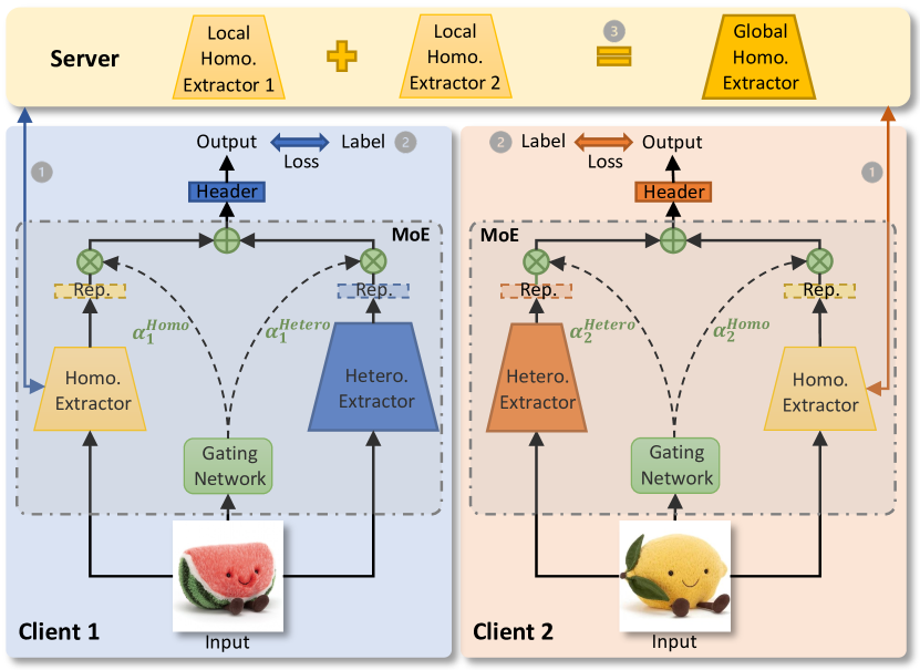
Figure 2. Workflow of pFedMoE.

Overview. To realize the above insights, pFedMoE incorporates a shareable small homogeneous feature extractor $\mathcal{G}(\theta)$ far smaller than the local heterogeneous feature extractor $\mathcal{F}_{k}^{ex}(\omega_{k}^{ex})$. As shown in Figure. 2, in the $t$-th communication round, the workflow of pFedMoE involves the following steps:

1. The server samples $K$ clients $\bm{\mathcal{S}^{t}}$ and sends the global homogeneous small feature extractor $\mathcal{G}(\theta^{{t}-{1}})$ aggregated in the $(t-1)$-th round to them.

2. Client $k\in\bm{\mathcal{S}^{t}}$ regards the received global homogeneous small feature extractor $\mathcal{G}(\theta^{{t}-{1}})$ as the global expert for extracting generalized feature across all classes, and treats the local heterogeneous large feature extractor $\mathcal{F}_{k}^{ex}(\omega_{k}^{ex,t-1})$ as the local expert for extracting personalized feature of local seen classes. A homogeneous or heterogeneous lightweight personalized local gating network $\mathcal{H}(\varphi_{k}^{t-1})$ is introduced to balance generalization and personalization by dynamically producing weights for each sample’s representations from two experts. The three models form an MoE architecture. The weighted mixed representation from MoE is then processed by the local heterogeneous large model’s prediction header $\mathcal{F}_{k}^{hd}(\omega_{k}^{hd,t-1})$ to extract personalized prediction information. The three models in MoE and the header are trained simultaneously in an end-to-end manner. The updated homogeneous $\mathcal{G}(\theta_{k}^{t})$ is uploaded to the server, while $\mathcal{F}_{k}(\omega_{k}^{t})$, $\mathcal{H}(\varphi_{k}^{t})$ are retained by the clients.

3. The server aggregates the received local homogeneous feature extractors $\mathcal{G}(\theta_{k}^{t})$ ($k\in\bm{\mathcal{S}^{t}}$) by weighted averaging to produce a new global homogeneous feature extractor $\mathcal{G}(\theta^{t})$.

The above process iterates until all local heterogeneous complete models (MoE and prediction header) converge. At the end of FL, local heterogeneous complete models are used for inference. The details of pFedMoE are illustrated in Algorithm 1 (Appendix A).

4.1. MoE Training

In the MoE, each local data sample $(\bm{x}_{i},y_{i})\in D_{k}$ is fed into the global expert $\mathcal{G}(\theta^{{t}-\mathbf{1}})$ to produce the generalized representation, and simultaneously into the local expert $\mathcal{F}_{k}^{ex}(\omega_{k}^{ex,t-1})$ to generate the personalized representation,

(3) $$\bm{\mathcal{R}}_{k,i}^{\mathcal{G},t}=\mathcal{G}(\bm{x}_{i};\theta^{t-1}),\bm{\mathcal{R}}_{k,i}^{\mathcal{F}_{k},t}=\mathcal{F}_{k}^{ex}(\bm{x}_{i};\omega_{k}^{ex,t-1}).$$

Each local data sample $(\bm{x}_{i},y_{i})\in D_{k}$ is also fed into the local gating network $\mathcal{H}(\varphi_{k}^{t-1})$ to produce weights for the two experts,

(4) $$[\alpha_{k,i}^{\mathcal{G},t},\alpha_{k,i}^{\mathcal{F}_{k},t}]=\mathcal{H}(\bm{x}_{i};\varphi_{k}^{t-1}),s.t.\ \alpha_{k,i}^{\mathcal{G},t}+\alpha_{k,i}^{\mathcal{F}_{k},t}=1.$$

Notice that different clients can hold heterogeneous gating networks $\mathcal{H}_{k}(\varphi_{k})$, with the same input dimension $d$ as the local data sample $\bm{x}$ and the same output dimension $h=2$. For simplicity of discussion, we use the same gating network $\mathcal{H}(\varphi_{k})$ for all clients.

Then, we mix the representations of two experts with the weights produced by the gating network,

(5) $$\bm{\mathcal{R}}_{k,i}^{t}=\alpha_{k,i}^{\mathcal{G},t}\cdot\bm{\mathcal{R}}_{k,i}^{\mathcal{G},t}+\alpha_{k,i}^{\mathcal{F}_{k},t}\cdot\bm{\mathcal{R}}_{k,i}^{\mathcal{F}_{k},t}.$$

To enable the above representation mixture, we require that the last layer dimensions of the homogeneous small feature extractor and the heterogeneous large feature extractor are identical. The mixed representation $\bm{\mathcal{R}}_{k,i}^{t}$ is then processed by the local personalized perdition header $\mathcal{F}_{k}^{hd}(\omega_{k}^{hd,t-1})$ (both homogeneous and heterogeneous headers are allowed, we use homogeneous headers in this work) to produce the prediction,

(6) $$\hat{y}_{i}=\mathcal{F}_{k}^{hd}(\bm{\mathcal{R}}_{k,i}^{t};\omega_{k}^{hd,t-1}).$$

We compute the hard loss (e.g. Cross-Entropy loss (Zhang and Sabuncu, 2018)) between the prediction and the label as:

(7) $$\ell_{i}=CE(\hat{y}_{i},y_{i}).$$

Then, we update all models simultaneously via gradient descent (e.g., SGD optimizer (Ruder, 2016)) in an end-to-end manner,

(8) $$\theta_{k}^{t} \leftarrow\theta^{t-1}-\eta_{\theta}\nabla\ell_{i},$$

$$\omega_{k}^{t} \leftarrow\omega_{k}^{t-1}-\eta_{\omega}\nabla\ell_{i},$$

$$\varphi_{k}^{t} \leftarrow\varphi_{k}^{t-1}-\eta_{\varphi}\nabla\ell_{i},$$

where $\eta_{\theta},\eta_{\omega},\eta_{\varphi}$ are the learning rates of the homogeneous small feature extractor, the heterogeneous large model, and the gating network. To enable stable convergence, we set $\eta_{\theta}=\eta_{\omega}$.

4.2. Homogeneous Extractor Aggregation

After local training, $k$ uploads its local homogeneous small feature extractor $\theta_{k}^{t}$ to the server. The server then aggregates them by weighted averaging to produce a new global feature extractor:

(9) $$\theta^{t}=\sum_{k\in\bm{\mathcal{S}^{t}}}\frac{n_{k}}{n}\theta_{k}^{t}.$$

Problem Re-formulation. The local personalized gating networks of different clients dynamically produce weights for the representations of two experts on each sample of local non-IID data, balancing generalization and personalization based on local data distributions. Thus, pFedMoE enhances personalization of model-heterogeneous personalized FL at the fine-grained data level. Therefore, the objective defined in Eq. (2) can be specified as:

(10) $$\footnotesize\min_{\omega_{0,\ldots,N-1}}\sum_{k=0}^{N-1}\ell(\mathcal{F}_{k}^{hd}((\mathcal{G}(D_{k};\theta),\mathcal{F}_{k}^{ex}(D_{k};\omega_{k}^{ex}))\cdot\bm{\mathcal{H}({D}_{k};{\varphi}_{k})};\omega_{k}^{hd})).$$

$\bm{\mathcal{H}({D}_{k};{\varphi}_{k})}$ denotes the weights $[\alpha^{\mathcal{G}},\alpha^{\mathcal{F}_{k}}]$ of two experts. $\cdot$ is dot product (i.e., summing after element-wise multiplication).

4.3. Gating Network Design

The local gating network $\mathcal{H}(\varphi_{k})$ takes each data sample $\bm{x}_{i}\in D_{k}$ as the input, and outputs two weights ${[\alpha}_{k,i}^{\mathcal{G}},\alpha_{k,i}^{\mathcal{F}_{k}}]$ (summing to $1$) for the representations of the two experts, as defined in Eq. (4). A linear network is the simplest model to fulfill these functions. Therefore, we customize a dedicated lightweight linear gating network for pFedMoE, depicted in Figure 3.

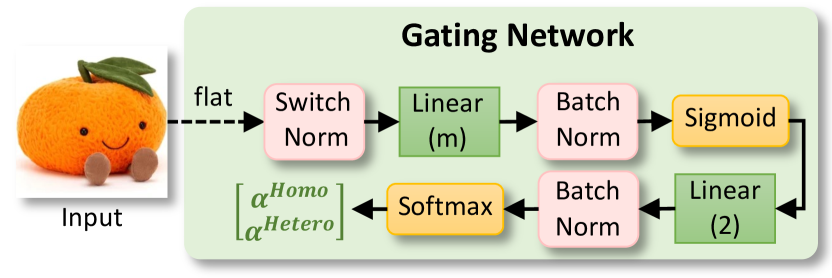
Figure 3. Gating network structure.

Linear Layer. pFedMoE trains models in batches. When processing a batch of color image samples, the input dimension is $[length,width,$ $channel=3,batchsize]$. Before feeding it into the gating network, we flatten it to a vector with $[(length\cdot width\cdot 3,batchsize])$ pixels. Given the large input vector, a gating network with only one linear layer containing $2$ neurons might not efficiently capture local data knowledge and could be prone to overfitting due to limited parameter capacity. Hence, we employ $2$ linear layers for the gating network: the first layer with $m$ neurons ($length\cdot width\cdot 3\cdot m$ parameters), and the second layer with $2$ neurons ($m\cdot 2$ parameters).

Normalization. Normalization techniques are commonly employed in deep neuron networks for regularization to improve model generalization and accelerate training. Common approaches include batch, instance, and layer normalization. Recently, switch normalization (Luo et al., 2019) integrates the advantages of these typical methods and efficiently handles batch data with diverse characteristics (Chen et al., 2023). After flattening the input, we apply a switch normalization layer before feeding it into the first linear layer. To leverage the benefits of widely adopted batch normalization, we include batch normalization layers after two linear layers.

Activation Function. Activation functions increase non-linearity to improve deep network expression, mitigating gradient vanishing or explosion. Commonly used activation functions include Sigmoid, ReLU, and Softmax, each with its range of values. Since the gating network’s output weights range between $0$ and $1$, we add a Sigmoid activation layer after the first linear layer to confine its output within $(0,1)$. We add a Softmax activation layer after the second linear layer to ensure that the produced two weights sum to $1$.

4.4. Discussion

Here, we further discuss the following aspects of pFedMoE.

Privacy. Clients share the homogeneous small feature extractors for knowledge exchange. Local heterogeneous large models and local data remain with the clients, thereby preserving their privacy.

Communication. Only homogeneous small feature extractors are transmitted between the server and clients, incurring lower communication costs than transmitting complete models as in FedAvg.

Computation. Apart from training local heterogeneous large models, clients also train a small homogeneous feature extractor and a lightweight linear gating network. However, due to their smaller sizes than the heterogeneous large feature extractor, the computation costs are acceptable. Moreover, simultaneous training of MoE and the prediction header reduces training time.

5. Analysis

We first clarify additional notations used for analysis in Table 1.

Table 1. Description of Additional Notations.

Notation	Description
$t\in\{0,\ldots,T-1\}$	communication round
$e\in\{0,1,\ldots,E\}$	local iteration
$tE+0$	before the $(t+1)$-th round’s local training, client $k$ receives the global homogeneous small feature extractor $\mathcal{G}(\theta^{t})$ aggregated in the $t$-th round
$tE+e$	the $e$-th local iteration in the $(t+1)$-th round
$tE+E$	the last local iteration, after that, client $k$ uploads the local homogeneous small feature extractor to the server
$W_{k}$	client $k$’s local complete model involving the MoE $\{\mathcal{G}(\theta),\mathcal{F}_{k}^{ex}(\omega_{k}^{ex}),\mathcal{H}(\varphi_{k})\}$ and the perdition header $\mathcal{F}_{k}^{hd}(\omega_{k}^{hd})$
$\eta$	the learning rate of the client $k$’s local complete model $W_{k}$, involving $\{\eta_{\theta},\eta_{\omega},\eta_{\varphi}\}$

Assumption 1.

Lipschitz Smoothness. Gradients of client $k$’s local complete heterogeneous model $W_{k}$ are $L1$–Lipschitz smooth (Tan et al., 2022),

(11) $$\footnotesize\begin{gathered}\|\nabla\mathcal{L}_{k}^{t_{1}}(W_{k}^{t_{1}};\bm{x},y)-\nabla\mathcal{L}_{k}^{t_{2}}(W_{k}^{t_{2}};\bm{x},y)\|\leqslant L_{1}\|W_{k}^{t_{1}}-W_{k}^{t_{2}}\|,\\ \forall t_{1},t_{2}>0,k\in\{0,1,\ldots,N-1\},(\bm{x},y)\in D_{k}.\end{gathered}$$

The above formulation can be further derived as:

(12) $$\footnotesize\mathcal{L}_{k}^{t_{1}}-\mathcal{L}_{k}^{t_{2}}\leqslant\langle\nabla\mathcal{L}_{k}^{t_{2}},(W_{k}^{t_{1}}-W_{k}^{t_{2}})\rangle+\frac{L_{1}}{2}\|W_{k}^{t_{1}}-W_{k}^{t_{2}}\|_{2}^{2}.$$

Assumption 2.

Unbiased Gradient and Bounded Variance. Client $k$’s random gradient $g_{W,k}^{t}=\nabla\mathcal{L}_{k}^{t}(W_{k}^{t};\mathcal{B}_{k}^{t})$ ($\mathcal{B}$ is a batch of local data) is unbiased,

(13) $$\footnotesize\mathbb{E}_{\mathcal{B}_{k}^{t}\subseteq D_{k}}[g_{W,k}^{t}]=\nabla\mathcal{L}_{k}^{t}(W_{k}^{t}),$$

and the variance of random gradient $g_{W,k}^{t}$ is bounded by:

(14) $$\footnotesize\begin{split}\mathbb{E}_{\mathcal{B}_{k}^{t}\subseteq D_{k}}[\|\nabla\mathcal{L}_{k}^{t}(W_{k}^{t};\mathcal{B}_{k}^{t})-\nabla\mathcal{L}_{k}^{t}(W_{k}^{t})\|_{2}^{2}]\leqslant\sigma^{2}.\end{split}$$

Assumption 3.

Bounded Parameter Variation. The parameter variations of the homogeneous small feature extractor $\theta_{k}^{t}$ and $\theta^{t}$ before and after aggregation is bounded as

(15) $$\footnotesize{\|\theta^{t}-\theta_{k}^{t}\|}_{2}^{2}\leq\delta^{2}.$$

Based on the above assumptions, we can derive the following Lemma and Theorem. Detailed proofs are given in Appendix B.

Lemma 0.

Local Training. Given Assumptions 1 and 2, the loss of an arbitrary client’s local model $W$ in the $(t+1)$-th local training round is bounded by

(16) $$\footnotesize\mathbb{E}[\mathcal{L}_{(t+1)E}]\leq\mathcal{L}_{tE+0}+(\frac{L_{1}\eta^{2}}{2}-\eta)\sum_{e=0}^{E}\|\nabla\mathcal{L}_{tE+e}\|_{2}^{2}+\frac{L_{1}E\eta^{2}\sigma^{2}}{2}.$$

Lemma 0.

Model Aggregation. Given Assumptions 2 and 3, after the $(t+1)$-th local training round, the loss of any client before and after aggregating local homogeneous small feature extractors at the server is bounded by

(17) $$\footnotesize\mathbb{E}\left[\mathcal{L}_{(t+1)E+0}\right]\leq\mathbb{E}\left[\mathcal{L}_{tE+1}\right]+{\eta\delta}^{2}.$$

Theorem 3.

One Complete Round of FL. Based on Lemma 1 and Lemma 2, for any client, after local training, model aggregation, and receiving the new global homogeneous feature extractor, we get

(18) $$\footnotesize\mathbb{E}[\mathcal{L}_{(t+1)E+0}]\leq\mathcal{L}_{tE+0}+(\frac{L_{1}\eta^{2}}{2}-\eta)\sum_{e=0}^{E}\|\nabla\mathcal{L}_{tE+e}\|_{2}^{2}+\frac{L_{1}E\eta^{2}\sigma^{2}}{2}+\eta\delta^{2}.$$

Theorem 4.

Non-convex Convergence Rate of pFedMoE. Based on Theorem 3, for any client and an arbitrary constant $\epsilon>0$, the following holds true:

(19) $$\frac{1}{T}\sum_{t=0}^{T-1}\sum_{e=0}^{E-1}\|\nabla\mathcal{L}_{tE+e}\|_{2}^{2} \leq\frac{\frac{1}{T}\sum_{t=0}^{T-1}[\mathcal{L}_{tE+0}-\mathbb{E}[\mathcal{L}_{(t+1)E+0}]]+\frac{L_{1}E\eta^{2}\sigma^{2}}{2}+\eta\delta^{2}}{\eta-\frac{L_{1}\eta^{2}}{2}}<\epsilon,$$

$$s.t. \eta<\frac{2(\epsilon-\delta^{2})}{L_{1}(\epsilon+E\sigma^{2})}.$$

Therefore, we conclude that any client’s local model can converge at a non-convex rate $\epsilon\sim\mathcal{O}(\frac{1}{T})$ under pFedMoE.

6. Experimental Evaluation

To evaluate the effectiveness of pFedMoE, we implement it and $7$ state-of-the-art baselines by Pytorch and compare them over 2 benchmark datasets on $4$ NVIDIA GeForce RTX 3090 GPUs.

6.1. Experiment Setup

Datasets. We evaluate pFedMoE and baselines on CIFAR-10 and CIFAR-100 (Krizhevsky et al., 2009) image classification benchmark datasets. CIFAR-10 comprises $6,000$ $32\times 32$ color images across $10$ classes, with $5,000$ images in the training set and $1,000$ images in the testing set. CIFAR-100 contains $100$ classes of color images, each with $500$ training images and $100$ testing images. To construct non-IID datasets, we adopt two data partitioning strategies: (1) Pathological: Following (Shamsian et al., 2021), we allocate $2$ classes to each client on CIFAR-10 and use Dirichlet distribution to generate varying counts of the same class for different clients, denoted as (non-IID: 2/10). We assign $10$ classes to each client on CIFAR-100, marked as (non-IID: 10/100). (2) Practical: Following Qin et al. (2023), we allocate all classes to each client and utilize Dirichlet distribution($\gamma$) to control the proportions of each class across clients. After non-IID division, each client’s local dataset is divided into training and testing sets in an $8:2$ ratio, ensuring both sets follow the same distribution.

Base Models. We assess pFedMoE and baselines in both model-homogeneous and model-heterogeneous FL scenarios. For model-homogeneous settings, all clients hold the same CNN-1 shown in Table 4 (Appendix C). In model-heterogeneous settings, $5$ heterogeneous CNN models are evenly allocated to different clients, with assignment IDs determined by client ID modulo $5$.

Comparison Baselines. We compare pFedMoE against state-of-the-art MHPFL algorithms from the three most relevant categories of public data-independent MHPFL algorithms outlined in Section 2.

• Standalone. Clients only utilize their local data to train models without FL process.

• MHPFL by Knowledge Distillation: FD (Jeong et al., 2018), FedProto (Tan et al., 2022).

• MHPFL by Model Mixture: LG-FedAvg (Liang et al., 2020).

• MHPFL by Mutual Learning: FML (Shen et al., 2020), FedKD (Wu et al., 2022), and the latest FedAPEN (Qin et al., 2023). pFedMoE belongs to this category.

Evaluation Metrics. We measure the model performance, communication cost, and computational overhead of all algorithms.

• Model Performance. We evaluate each client’s local model’s individual test accuracy (%) on the local testing set and calculate their mean test accuracy.

• Communication Cost. We monitor the communication rounds required to reach target mean accuracy and quantify communication costs by multiplying rounds with the mean parameter capacity transmitted in one round.

• Computation Overhead. We calculate computation overhead by multiplying the communication rounds required to achieve target mean accuracy with the local mean computational FLOPs in one round.

Training Strategy. We conduct a grid search to identify the optimal FL settings and specific hyperparameters for all algorithms. In FL settings, we evaluate all algorithms over $T=\{100,500\}$ communication rounds, $\{1,10\}$ local epochs, $\{64,128,256,512\}$ batch sizes, and the SGD optimizer with learning rate $\{0.001,0.01,0.1,1\}$. For pFedMoE, the homogeneous small feature extractor and the heterogeneous large model have the same learning rate (i.e., $\eta_{\theta}=\eta_{\omega}$). We report the highest accuracy achieved by all algorithms.

6.2. Results and Discussion

To test algorithms in different FL scenarios with diverse number of clients $N$ and client participation rates $C$, we design three settings: $\{(N=10,C=100\%),(N=50,C=20\%),(N=100,C=10\%)\}$.

6.2.1. Model Homogeneity

Table 2 shows that pFedMoE consistently achieves the highest accuracy, surpassing each setting’s state-of-the-art baseline (LG-FedAvg, Standalone, Standalone, FedProto, Standalone, Standalone) by up to $1.74\%$, and improving the accuracy by up to $5.47\%$ compared with the same-category best baseline (FedAPEN, FedAPEN, FedAPEN, FedAPEN, FedKD, FedKD). The results indicate that pFedMoE efficiently boosts model accuracy through adaptive data-level personalization.

6.2.2. Model Heterogeneity

In this scenario, pFedMoE and other mutual learning-based MHPFL baselines utilize the smallest CNN-5 (Table 4, Appendix C) as homogeneous feature extractors or models.

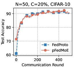
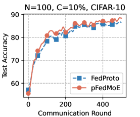
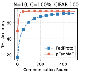
Figure 11. Average accuracy vs. communication rounds.

Mean Accuracy. Table 3 shows that pFedMoE consistently outperforms other baselines, improving test accuracy by up to $2.80\%$ compared to the state-of-the-art baseline under each setting (Standalone, FedProto, FedProto, Standalone, FedProto, FedProto). It improves test accuracy by up to $22.16\%$ compared to the same-category best baseline (FedKD). Figure 11 (Appendix C) shows that pFedMoE achieves faster convergence and higher model accuracy across most FL settings, particularly noticeable on CIFAR-100.

Individual Accuracy. Figure 4 shows the performance variance of pFedMoE and the state-of-the-art baseline - FedProto in terms of the individual accuracy of each client under ($N=100,C=10\%$). Most clients (CIFAR-10: $76\%$, CIFAR-100: $60\%$) with pFedMoE achieve higher accuracy than FedProto. This demonstrates that pFedMoE with data-level personalization dynamically adapts to local data distribution and learns more generalized and personalized knowledge from local data.

Table 2. Mean accuracy in model-homogeneous FL scenarios.

FL Setting	N=10, C=100%		N=50, C=20%		N=100, C=10%
Method	CIFAR-10	CIFAR-100	CIFAR-10	CIFAR-100	CIFAR-10	CIFAR-100
Standalone	96.35	74.32	95.25	62.38	92.58	54.93
LG-FedAvg (Liang et al., 2020)	96.47	73.43	94.20	61.77	90.25	46.64
FD (Jeong et al., 2018)	96.30	-	-	-	-	-
FedProto (Tan et al., 2022)	95.83	72.79	95.10	62.55	91.19	54.01
FML (Shen et al., 2020)	94.83	70.02	93.18	57.56	87.93	46.20
FedKD (Wu et al., 2022)	94.77	70.04	92.93	57.56	90.23	50.99
FedAPEN (Qin et al., 2023)	95.38	71.48	93.31	57.62	87.97	46.85
pFedMoE	96.80	76.06	95.80	63.06	93.55	56.46
pFedMoE-Best B.	0.33	1.74	0.55	0.51	0.97	1.53
pFedMoE-Best S.C.B.	1.42	4.58	2.49	5.44	3.32	5.47

Note: “-” denotes failure to converge. “Best B.” indicates the best baseline. “Best S.C.B.” means the best same-category baseline.

Table 3. Mean accuracy in model-heterogeneous FL scenarios.

FL Setting	N=10, C=100%		N=50, C=20%		N=100, C=10%
Method	CIFAR-10	CIFAR-100	CIFAR-10	CIFAR-100	CIFAR-10	CIFAR-100
Standalone	96.53	72.53	95.14	62.71	91.97	53.04
LG-FedAvg (Liang et al., 2020)	96.30	72.20	94.83	60.95	91.27	45.83
FD (Jeong et al., 2018)	96.21	-	-	-	-	-
FedProto (Tan et al., 2022)	96.51	72.59	95.48	62.69	92.49	53.67
FML (Shen et al., 2020)	30.48	16.84	-	21.96	-	15.21
FedKD (Wu et al., 2022)	80.20	53.23	77.37	44.27	73.21	37.21
FedAPEN (Qin et al., 2023)	-	-	-	-	-	-
pFedMoE	96.58	75.39	95.84	63.30	93.07	54.78
pFedMoE-Best B.	0.05	2.80	0.36	0.59	0.58	1.11
pFedMoE-Best S.C.B.	16.38	22.16	18.47	19.03	19.86	17.57

Note: “-” denotes failure to converge. “Best B.” indicates the best baseline. “Best S.C.B.” means the best same-category baseline.

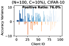
Figure 4. Accuracy distribution for individual clients.

Personalization Analysis. To explore the personalization level of pFedMoE and FedProto, we extract the representation of each local data sample from each client produced by pFedMoE’s local heterogeneous MoE and FedProto’s local heterogeneous feature extractor on CIFAR-10 (non-IID: 2/10) under ($N=100,C=10\%$). We adopt T-SNE (van der Maaten and Hinton, 2008) to compress extracted representations to $2$-dimension vectors and visualize them in Figure 5. Limited by plotting spaces, more clients $N=\{50,100\}$ and CIFAR-100 with $100$ classes cannot be clearly depicted. Figure 5 shows that representations from one client’s $2$ seen classes are close together, while representations from different clients are further apart, indicating that two algorithms indeed yield personalized local heterogeneous models. Regarding representations of one client’s $2$ classes, they present “intra-class compactness, inter-class separation”, signifying a strong classification capability. Notably, representations of one client’s $2$ classes under pFedMoE exhibit clearer decision boundaries (i.e., representations within the same cluster are more compact), suggesting high classification performance and personalization .

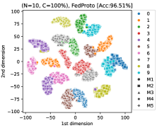
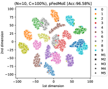
Figure 5. T-SNE representation visualization results for FedProto and pFedMoE on CIFAR-10 (non-IID: 2/10).

Overhead Analysis. Figure 6 shows the required number of rounds, communication, and computation costs for pFedMoE and FedProto to reach $90\%$ and $50\%$ test accuracy under the most complex ($N=100,C=10\%$) setting. For fair comparisons, we normalize communication and computation costs, considering only their different dimensions (i.e., number of parameters, FLOPs).

Computation. pFedMoE incurs lower computational costs than FedProto. This is because FedProto requires extracting representations for all local data samples after training local heterogeneous models, while pFedMoE trains an MoE and the prediction header simultaneously. One round of computation in pFedMoE is less than FedProto. Since pFedMoE also requires fewer rounds to reach the target accuracy, it incurs lower total computation costs.

Communication. pFedMoE incurs higher communication costs than FedProto. This is because in one round, clients with FedProto transmit seen-class representations to the server, while clients with pFedMoE transmit homogeneous small feature extractors. This, the former consumes lower communication costs per round. Despite requiring fewer rounds to reach the target accuracy, pFedMoE still consumes higher total communication costs. However, compared with transmitting complete local models in FedAvg, pFedMoE still incurs lower communication overheads. Therefore, pFedMoE achieves highly efficient computation with acceptable communication costs, while delivering superior model accuracy.

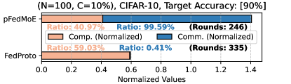
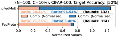
Figure 6. Computation (Comp.), communication (Comm.), and rounds required for reaching target mean accuracy.

6.3. Case Studies

6.3.1. Robustness to Pathological Non-IIDness

In model heterogeneous FL with ($N=100,C=10\%$), the number of seen classes assigned to one client varies as $\{2,4,6,8,10\}$ on CIFAR-10 and $\{10,30,50,70,90,100\}$ on CIFAR-100. Figure 7 shows that model accuracy drops as non-IIDness reduces (number of seen classes rises), as clients with more classes exhibit degraded classification ability for each class (i.e., model generalization improves, but personalization drops). Besides, pFedMoE consistently achieves higher test accuracy than FedProto across various non-IIDnesses settings, indicating its robustness to pathological non-IIDness. Moreover, pFedMoE achieves higher accuracy improvements compared to FedProto under IID settings than under non-IID settings, e.g., $+13.10\%$ on CIFAR-10 (non-IID: 8/10) and $+3.04\%$ on CIFAR-100 (non-IID: 30/100). This suggests that FedProto is more effective under non-IID settings than under IID settings, consistent with the behavior of most personalized FL algorithms (Qin et al., 2023). In contrast, pFedMoE adapts to both IID and non-IID settings by the personalized gating network to dynamically balance global generalization and local personalization.

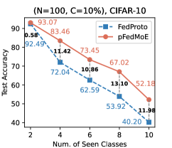
Figure 7. Robustness to pathological non-IIDness.

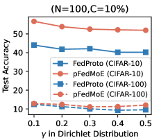
Figure 8. Left: robustness to practical non-IIDness. Right: sensitivity to the gating network learning rate.

6.3.2. Robustness to Practical Non-IIDness

In model heterogeneous FL with ($N=100,C=10\%$), $\gamma$ of the Dirichlet distribution varies as $\{0.1,0.2,0.3,0.4,0.5\}$. Figure 8(left) shows that pFedMoE consistently achieves higher accuracy than FedProto, indicating its robustness to practical non-IIDness. Similar to Figure 7, model accuracy drops as non-IIDness reduces ($\gamma$ rises). pFedMoE improves test accuracy more under IID settings than under non-IID settings.

6.3.3. Sensitivity Analysis

Only one extra hyperparameter, the learning rate $\eta_{\varphi}$ of the gating network, is introduced by pFedMoE. In model heterogeneous FL with ($N=100,C=10\%$), we evaluate pFedMoE with $\eta_{\varphi}=\{0.001,0.01,0.1,1\}$ on CIFAR-10 (non-IID: 2/10) and CIFAR-100 (non-IID: 10/100). We select three random seeds to execute $3$ trails for each test. Figure 8 (right) shows the accuracy mean (dots) and variation (shadow). pFedMoE achieves stable accuracy across various gating network learning rates, indicating that it is not sensitive to $\eta_{\varphi}$.

6.3.4. Weight Analysis

We analyze pFedMoE’s gating network output weights in a model heterogeneous FL with ($N=100,C=10\%$) on CIFAR-10 (non-IID: 2/10) and CIFAR-100 (non-IID: 10/100).

Client Perspective. We randomly select $5$ clients and visualize the probability distribution of the weights produced by the final local gating network for the local personalized heterogeneous large feature extractor on all local testing data. Figure 9 shows that different clients with non-IID data exhibit diverse weight distributions, indicating that the weights produced by the local personalized gating network for different clients are indeed personalized to local data distributions. Besides, most weights are concentrated around $50\%$, with some exceeding $50\%$, suggesting that the generalized features extracted by the small homogeneous feature extractor and the personalized features extracted by the large heterogeneous feature extractor contribute comparably to model performance. The personalized output weights dynamically balance generalization and personalization.

Class Perspective. Upon identifying client sets with the same seen classes, we find $4$ clients sharing classes $[1,2]$, and $3$ clients sharing classes $[3,8]$ on CIFAR-10. However, no pair of clients have overlapping seen classes on CIFAR-100 as $100$ classes are assigned to $100$ clients. Figure 10 shows that one class across different clients performs various weight distributions and different classes within one client also exhibit diverse weight distributions, highlighting that pFedMoE indeed achieves data-level personalization.

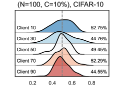
Figure 9. Produced weight distributions vary as clients.

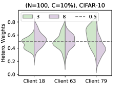
Figure 10. Produced weight distributions vary as classes.

7. Conclusions and Future Work

In this paper, we proposed a novel model-heterogeneous personalized federated learning algorithm, pFedMoE, to achieve data-level personalization by leveraging a mixture of experts (MoE). Each client’s local complete model consists of a heterogeneous MoE (a share homogeneous small feature extractor (global expert), a local heterogeneous large model’s feature extractor (local expert), a local personalized gating network) and a local heterogeneous large model’s personalized prediction header. pFedMoE exchanges knowledge from local heterogeneous models across different clients by sharing homogeneous small feature extractors, and it achieves data-level personalization adaptive to local non-IID data distribution by MoE to balance generalization and personalization. Theoretical analysis proves its $\mathcal{O}(1/T)$ non-convex convergence rate. Extensive experiments demonstrate that pFedMoE obtains the state-of-the-art model accuracy with lower computation overheads and acceptable communication costs.

In subsequent research, we will explore how pFedMoE performs in federated continuous learning (FCL) scenarios involving steaming data with distribution drift.

Appendix A Pseudo codes of pFedMoE

Input: $N$, total number of clients; $K$, number of sampled clients in one round; $T$, number of rounds; $\eta_{\theta}$, learning rate of homogeneous feature extractor; $\eta_{\omega}$, learning rate of local heterogeneous models; $\eta_{\varphi}$, learning rate of local homogeneous gating network.

Randomly initialize the global homogeneous feature extractor $\mathcal{G}(\theta^{\mathbf{0}})$, local personalized heterogeneous models $[\mathcal{F}_{0}(\omega_{0}^{0}),\mathcal{F}_{1}(\omega_{1}^{0}),\ldots,\mathcal{F}_{k}(\omega_{k}^{0}),\ldots,\mathcal{F}_{N-1}(\omega_{N-1}^{0})]$ and local homogeneous gating networks $\mathcal{H}(\varphi^{\mathbf{0}})$.

for $t=1$ to $T-1$ do

       // Server Side:

       $\bm{\mathcal{S}}^{t}\leftarrow$ Randomly sample $K\leqslant N$ clients to join FL;

       Broadcast the global homogeneous feature extractor $\theta^{t-1}$ to sampled $K$ clients;

       $\theta_{k}^{t}\leftarrow$ Client Update$(\theta^{t-1})$;

      

      

       // Client Update:

       Receive the global homogeneous feature extractor $\theta^{t-1}$ from the server;

       for $k\in\bm{\mathcal{S}}^{t}$ do

             for $(\bm{x}_{i},y_{i})\in D_{k}$ do

                  

                  

                  

             end for

            Upload trained local homogeneous feature extractor $\theta_{k}^{t}$ to the server.

       end for

      

end for

Return personalized heterogeneous local complete models

Algorithm 1 pFedMoE

Appendix B Theoretical Proofs

B.1. Proof for Lemma 1

An arbitrary client $k$’s local model $W$ can be updated by $W_{t+1}=W_{t}-\eta g_{W,t}$ in the (t+1)-th round, and following Assumption 1, we can obtain

(20) $$\mathcal{L}_{tE+1} \leq\mathcal{L}_{tE+0}+\langle\nabla\mathcal{L}_{tE+0},(W_{tE+1}-W_{tE+0})\rangle+\frac{L_{1}}{2}\|W_{tE+1}-W_{tE+0}\|_{2}^{2}$$

$$=\mathcal{L}_{tE+0}-\eta\langle\nabla\mathcal{L}_{tE+0},g_{W,tE+0}\rangle+\frac{L_{1}\eta^{2}}{2}\|g_{W,tE+0}\|_{2}^{2}.$$

Taking the expectation of both sides of the inequality concerning the random variable $\xi_{tE+0}$, we obtain

(21) $$\mathbb{E}[\mathcal{L}_{tE+1}] \leq\mathcal{L}_{tE+0}-\eta\mathbb{E}[\langle\nabla\mathcal{L}_{tE+0},g_{W,tE+0}\rangle]+\frac{L_{1}\eta^{2}}{2}\mathbb{E}[\|g_{W,tE+0}\|_{2}^{2}]$$

$$\stackrel{{\scriptstyle(a)}}{{=}}\mathcal{L}_{tE+0}-\eta\|\nabla\mathcal{L}_{tE+0}\|_{2}^{2}+\frac{L_{1}\eta^{2}}{2}\mathbb{E}[\|g_{W,tE+0}\|_{2}^{2}]$$

$$\stackrel{{\scriptstyle(b)}}{{\leq}}\mathcal{L}_{tE+0}-\eta\|\nabla\mathcal{L}_{tE+0}\|_{2}^{2}+\frac{L_{1}\eta^{2}}{2}(\mathbb{E}[\|g_{W,tE+0}\|]_{2}^{2}+\operatorname{Var}(g_{W,tE+0}))$$

$$\stackrel{{\scriptstyle(c)}}{{=}}\mathcal{L}_{tE+0}-\eta\|\nabla\mathcal{L}_{tE+0}\|_{2}^{2}+\frac{L_{1}\eta^{2}}{2}(\|\nabla\mathcal{L}_{tE+0}\|_{2}^{2}+\operatorname{Var}(g_{W,tE+0}))$$

$$\stackrel{{\scriptstyle(d)}}{{\leq}}\mathcal{L}_{tE+0}-\eta\|\nabla\mathcal{L}_{tE+0}\|_{2}^{2}+\frac{L_{1}\eta^{2}}{2}(\|\nabla\mathcal{L}_{tE+0}\|_{2}^{2}+\sigma^{2})$$

$$=\mathcal{L}_{tE+0}+(\frac{L_{1}\eta^{2}}{2}-\eta)\|\nabla\mathcal{L}_{tE+0}\|_{2}^{2}+\frac{L_{1}\eta^{2}\sigma^{2}}{2}.$$

(a), (c), (d) follow Assumption 2. (b) follows $Var(x)=\mathbb{E}[x^{2}]-(\mathbb{E}[x]^{2})$.

Taking the expectation of both sides of the inequality for the model $W$ over $E$ iterations, we obtain

(22) $$\mathbb{E}[\mathcal{L}_{tE+1}]\leq\mathcal{L}_{tE+0}+(\frac{L_{1}\eta^{2}}{2}-\eta)\sum_{e=1}^{E}\|\nabla\mathcal{L}_{tE+e}\|_{2}^{2}+\frac{L_{1}E\eta^{2}\sigma^{2}}{2}.$$

B.2. Proof for Lemma 2

(23) $$\mathcal{L}_{(t+1)E+0} =\mathcal{L}_{(t+1)E}+\mathcal{L}_{(t+1)E+0}-\mathcal{L}_{(t+1)E}$$

$$\stackrel{{\scriptstyle(a)}}{{\approx}}\mathcal{L}_{(t+1)E}+\eta\|\theta_{(t+1)E+0}-\theta_{(t+1)E}\|_{2}^{2}$$

$$\stackrel{{\scriptstyle(b)}}{{\leq}}\mathcal{L}_{(t+1)E}+\eta\delta^{2}.$$

(a): we can use the gradient of parameter variations to approximate the loss variations, i.e., $\Delta\mathcal{L}\approx\eta\cdot\|\Delta\theta\|_{2}^{2}$. (b) follows Assumption 3.

Taking the expectation of both sides of the inequality to the random variable $\xi$, we obtain

(24) $$\mathbb{E}\left[\mathcal{L}_{(t+1)E+0}\right]\leq\mathbb{E}\left[\mathcal{L}_{tE+1}\right]+{\eta\delta}^{2}.$$

B.3. Proof for Theorem 3

Substituting Lemma 1 into the right side of Lemma 2’s inequality, we obtain

(25) $$\mathbb{E}[\mathcal{L}_{(t+1)E+0}]\leq\mathcal{L}_{tE+0}+(\frac{L_{1}\eta^{2}}{2}-\eta)\sum_{e=0}^{E}\|\nabla\mathcal{L}_{tE+e}\|_{2}^{2}+\frac{L_{1}E\eta^{2}\sigma^{2}}{2}+\eta\delta^{2}.$$

B.4. Proof for Theorem 4

Interchanging the left and right sides of Eq. (25), we obtain

(26) $$\sum_{e=0}^{E}\|\nabla\mathcal{L}_{tE+e}\|_{2}^{2}\leq\frac{\mathcal{L}_{tE+0}-\mathbb{E}[\mathcal{L}_{(t+1)E+0}]+\frac{L_{1}E\eta^{2}\sigma^{2}}{2}+\eta\delta^{2}}{\eta-\frac{L_{1}\eta^{2}}{2}}.$$

Taking the expectation of both sides of the inequality over rounds $t=[0,T-1]$ to $W$, we obtain

(27) $$\frac{1}{T}\sum_{t=0}^{T-1}\sum_{e=0}^{E-1}\|\nabla\mathcal{L}_{tE+e}\|_{2}^{2}\leq\frac{\frac{1}{T}\sum_{t=0}^{T-1}[\mathcal{L}_{tE+0}-\mathbb{E}[\mathcal{L}_{(t+1)E+0}]]+\frac{L_{1}E\eta^{2}\sigma^{2}}{2}+\eta\delta^{2}}{\eta-\frac{L_{1}\eta^{2}}{2}}.$$

Let $\Delta=\mathcal{L}_{t=0}-\mathcal{L}^{*}>0$, then $\sum_{t=0}^{T-1}[\mathcal{L}_{tE+0}-\mathbb{E}[\mathcal{L}_{(t+1)E+0}]]\leq\Delta$, we can get

(28) $$\frac{1}{T}\sum_{t=0}^{T-1}\sum_{e=0}^{E-1}\|\nabla\mathcal{L}_{tE+e}\|_{2}^{2}\leq\frac{\frac{\Delta}{T}+\frac{L_{1}E\eta^{2}\sigma^{2}}{2}+\eta\delta^{2}}{\eta-\frac{L_{1}\eta^{2}}{2}}.$$

If the above equation converges to a constant $\epsilon$, i.e.,

(29) $$\frac{\frac{\Delta}{T}+\frac{L_{1}E\eta^{2}\sigma^{2}}{2}+\eta\delta^{2}}{\eta-\frac{L_{1}\eta^{2}}{2}}<\epsilon,$$

then

(30) $$T>\frac{\Delta}{\epsilon(\eta-\frac{L_{1}\eta^{2}}{2})-\frac{L_{1}E\eta^{2}\sigma^{2}}{2}-\eta\delta^{2}}.$$

Since $T>0,\Delta>0$, we can get

(31) $$\epsilon(\eta-\frac{L_{1}\eta^{2}}{2})-\frac{L_{1}E\eta^{2}\sigma^{2}}{2}-\eta\delta^{2}>0.$$

Solving the above inequality yields

(32) $$\eta<\frac{2(\epsilon-\delta^{2})}{L_{1}(\epsilon+E\sigma^{2})}.$$

Since $\epsilon,\ L_{1},\ \sigma^{2},\ \delta^{2}$ are all constants greater than 0, $\eta$ has solutions. Therefore, when the learning rate $\eta$ satisfies the above condition, any client’s local complete heterogeneous model can converge. Notice that the learning rate of the local complete heterogeneous model involves $\{\eta_{\theta},\eta_{\omega},\eta_{\varphi}\}$, so it’s crucial to set reasonable them to ensure model convergence. Since all terms on the right side of Eq. (28) except for $\Delta/T$ are constants, $\Delta$ is also a constant, pFedMoE’s non-convex convergence rate is $\epsilon\sim\mathcal{O}(\frac{1}{T})$.

Appendix C More Experimental Details and Results

Table 4. Structures of $5$ heterogeneous CNN models with $5\times 5$ kernel size and $16$ or $32$ filters in convolutional layers.

Layer Name	CNN-1	CNN-2	CNN-3	CNN-4	CNN-5
Conv1	5$\times$5, 16	5$\times$5, 16	5$\times$5, 16	5$\times$5, 16	5$\times$5, 16
Maxpool1	2$\times$2	2$\times$2	2$\times$2	2$\times$2	2$\times$2
Conv2	5$\times$5, 32	5$\times$5, 16	5$\times$5, 32	5$\times$5, 32	5$\times$5, 32
Maxpool2	2$\times$2	2$\times$2	2$\times$2	2$\times$2	2$\times$2
FC1	2000	2000	1000	800	500
FC2	500	500	500	500	500
FC3	10/100	10/100	10/100	10/100	10/100
model size	10.00 MB	6.92 MB	5.04 MB	3.81 MB	2.55 MB

References

- (1)
- Ahn et al. (2019) Jin-Hyun Ahn et al. 2019. Wireless Federated Distillation for Distributed Edge Learning with Heterogeneous Data. In Proc. PIMRC. IEEE, Istanbul, Turkey, 1–6.
- Ahn et al. (2020) Jin-Hyun Ahn et al. 2020. Cooperative Learning VIA Federated Distillation OVER Fading Channels. In Proc. ICASSP. IEEE, Barcelona, Spain, 8856–8860.
- Alam et al. (2022) Samiul Alam et al. 2022. FedRolex: Model-Heterogeneous Federated Learning with Rolling Sub-Model Extraction. In Proc. NeurIPS. , virtual.
- Babakniya et al. (2023) Sara Babakniya et al. 2023. Revisiting Sparsity Hunting in Federated Learning: Why does Sparsity Consensus Matter? Transactions on Machine Learning Research (2023). https://openreview.net/forum?id=iHyhdpsnyi
- Chang et al. (2021) Hongyan Chang et al. 2021. Cronus: Robust and Heterogeneous Collaborative Learning with Black-Box Knowledge Transfer. In Proc. NeurIPS Workshop. , virtual.
- Chen et al. (2023) Daoyuan Chen et al. 2023. Efficient Personalized Federated Learning via Sparse Model-Adaptation. In Proc. ICML, Vol. 202. PMLR, Honolulu, Hawaii, USA, 5234–5256.
- Chen et al. (2021) Jiangui Chen et al. 2021. FedMatch: Federated Learning Over Heterogeneous Question Answering Data. In Proc. CIKM. ACM, virtual, 181–190.
- Cheng et al. (2021) Sijie Cheng et al. 2021. FedGEMS: Federated Learning of Larger Server Models via Selective Knowledge Fusion. CoRR abs/2110.11027 (2021).
- Cho et al. (2022) Yae Jee Cho et al. 2022. Heterogeneous Ensemble Knowledge Transfer for Training Large Models in Federated Learning. In Proc. IJCAI. ijcai.org, virtual, 2881–2887.
- Collins et al. (2021) Liam Collins et al. 2021. Exploiting Shared Representations for Personalized Federated Learning. In Proc. ICML, Vol. 139. PMLR, virtual, 2089–2099.
- Diao (2021) Enmao Diao. 2021. HeteroFL: Computation and Communication Efficient Federated Learning for Heterogeneous Clients. In Proc. ICLR. OpenReview.net, Virtual Event, Austria, 1.
- Dun et al. (2023) Chen Dun et al. 2023. FedJETs: Efficient Just-In-Time Personalization with Federated Mixture of Experts. arXiv:2306.08586 [cs.LG]
- Guo et al. (2021) Binbin Guo et al. 2021. PFL-MoE: Personalized Federated Learning Based on Mixture of Experts. In Proc. APWeb-WAIM, Vol. 12858. Springer, Guangzhou, China, 480–486.
- He et al. (2020) Chaoyang He et al. 2020. Group Knowledge Transfer: Federated Learning of Large CNNs at the Edge. In Proc. NeurIPS. , virtual.
- Horváth (2021) S. Horváth. 2021. FjORD: Fair and Accurate Federated Learning under heterogeneous targets with Ordered Dropout. In Proc. NIPS. OpenReview.net, Virtual, 12876–12889.
- Huang et al. (2022a) Wenke Huang et al. 2022a. Few-Shot Model Agnostic Federated Learning. In Proc. MM. ACM, Lisboa, Portugal, 7309–7316.
- Huang et al. (2022b) Wenke Huang et al. 2022b. Learn from Others and Be Yourself in Heterogeneous Federated Learning. In Proc. CVPR. IEEE, virtual, 10133–10143.
- Itahara et al. (2023) Sohei Itahara et al. 2023. Distillation-Based Semi-Supervised Federated Learning for Communication-Efficient Collaborative Training With Non-IID Private Data. IEEE Trans. Mob. Comput. 22, 1 (2023), 191–205.
- Jang et al. (2022) Jaehee Jang et al. 2022. FedClassAvg: Local Representation Learning for Personalized Federated Learning on Heterogeneous Neural Networks. In Proc. ICPP. ACM, virtual, 76:1–76:10.
- Jeong et al. (2018) Eunjeong Jeong et al. 2018. Communication-Efficient On-Device Machine Learning: Federated Distillation and Augmentation under Non-IID Private Data. In Proc. NeurIPS Workshop on Machine Learning on the Phone and other Consumer Devices. , virtual.
- Kairouz et al. (2021) Peter Kairouz et al. 2021. Advances and Open Problems in Federated Learning. Foundations and Trends in Machine Learning 14, 1–2 (2021), 1–210.
- Krizhevsky et al. (2009) Alex Krizhevsky et al. 2009. Learning multiple layers of features from tiny images. Toronto, ON, Canada, .
- Li and Wang (2019) Daliang Li and Junpu Wang. 2019. FedMD: Heterogenous Federated Learning via Model Distillation. In Proc. NeurIPS Workshop. , virtual.
- Li et al. (2021) Qinbin Li et al. 2021. Practical One-Shot Federated Learning for Cross-Silo Setting. In Proc. IJCAI. ijcai.org, virtual, 1484–1490.
- Li et al. (2020) Xiaoxiao Li et al. 2020. Multi-site fMRI analysis using privacy-preserving federated learning and domain adaptation: ABIDE results. Medical Image Anal. 65 (2020), 101765.
- Liang et al. (2020) Paul Pu Liang et al. 2020. Think locally, act globally: Federated learning with local and global representations. arXiv preprint arXiv:2001.01523 1, 1 (2020).
- Lin et al. (2020) Tao Lin et al. 2020. Ensemble Distillation for Robust Model Fusion in Federated Learning. In Proc. NeurIPS. , virtual.
- Liu et al. (2022) Chang Liu et al. 2022. Completely Heterogeneous Federated Learning. CoRR abs/2210.15865 (2022).
- Lu et al. (2022) Xiaofeng Lu et al. 2022. Heterogeneous Model Fusion Federated Learning Mechanism Based on Model Mapping. IEEE Internet Things J. 9, 8 (2022), 6058–6068.
- Luo et al. (2019) Ping Luo et al. 2019. Differentiable Learning-to-Normalize via Switchable Normalization. In Proc. ICLR. OpenReview.net, New Orleans, LA, USA, 1.
- Makhija et al. (2022) Disha Makhija et al. 2022. Architecture Agnostic Federated Learning for Neural Networks. In Proc. ICML, Vol. 162. PMLR, virtual, 14860–14870.
- McMahan et al. (2017) Brendan McMahan et al. 2017. Communication-Efficient Learning of Deep Networks from Decentralized Data. In Proc. AISTATS, Vol. 54. PMLR, Fort Lauderdale, FL, USA, 1273–1282.
- Nguyen et al. (2023) Duy Phuong Nguyen et al. 2023. Enhancing Heterogeneous Federated Learning with Knowledge Extraction and Multi-Model Fusion. In Proc. SC Workshop. ACM, Denver, CO, USA, 36–43.
- Oh et al. (2022) Jaehoon Oh et al. 2022. FedBABU: Toward Enhanced Representation for Federated Image Classification. In Proc. ICLR. OpenReview.net, virtual.
- Park et al. (2023) Sejun Park et al. 2023. Towards Understanding Ensemble Distillation in Federated Learning. In Proc. ICML, Vol. 202. PMLR, Honolulu, Hawaii, USA, 27132–27187.
- Pillutla et al. (2022) Krishna Pillutla et al. 2022. Federated Learning with Partial Model Personalization. In Proc. ICML, Vol. 162. PMLR, virtual, 17716–17758.
- Qin et al. (2023) Zhen Qin et al. 2023. FedAPEN: Personalized Cross-silo Federated Learning with Adaptability to Statistical Heterogeneity. In Proc. KDD. ACM, Long Beach, CA, USA, 1954–1964.
- Reisser et al. (2021) Matthias Reisser et al. 2021. Federated Mixture of Experts. CoRR abs/2107.06724 (2021), 1.
- Ruder (2016) Sebastian Ruder. 2016. An overview of gradient descent optimization algorithms. CoRR abs/1609.04747 (2016), 1.
- Sattler et al. (2021) Felix Sattler et al. 2021. FEDAUX: Leveraging Unlabeled Auxiliary Data in Federated Learning. IEEE Trans. Neural Networks Learn. Syst. 1, 1 (2021), 1–13.
- Sattler et al. (2022) Felix Sattler et al. 2022. CFD: Communication-Efficient Federated Distillation via Soft-Label Quantization and Delta Coding. IEEE Trans. Netw. Sci. Eng. 9, 4 (2022), 2025–2038.
- Shamsian et al. (2021) Aviv Shamsian et al. 2021. Personalized Federated Learning using Hypernetworks. In Proc. ICML, Vol. 139. PMLR, virtual, 9489–9502.
- Shen et al. (2020) Tao Shen et al. 2020. Federated Mutual Learning. CoRR abs/2006.16765 (2020).
- Tan et al. (2022) Yue Tan et al. 2022. FedProto: Federated Prototype Learning across Heterogeneous Clients. In Proc. AAAI. AAAI Press, virtual, 8432–8440.
- van der Maaten and Hinton (2008) Laurens van der Maaten and Geoffrey Hinton. 2008. Visualizing Data using t-SNE. Journal of Machine Learning Research 9, 86 (2008), 2579–2605.
- Wang et al. (2023) Jiaqi Wang et al. 2023. Towards Personalized Federated Learning via Heterogeneous Model Reassembly. In Proc. NeurIPS. OpenReview.net, New Orleans, Louisiana, USA, 13.
- Wu et al. (2022) Chuhan Wu et al. 2022. Communication-efficient federated learning via knowledge distillation. Nature Communications 13, 1 (2022), 2032.
- Yi et al. (2023) Liping Yi, Gang Wang, Xiaoguang Liu, Zhuan Shi, and Han Yu. 2023. FedGH: Heterogeneous Federated Learning with Generalized Global Header. In Proceedings of the 31st ACM International Conference on Multimedia (ACM MM’23). ACM, Canada, 11.
- Yu et al. (2021) Fuxun Yu et al. 2021. Fed2: Feature-Aligned Federated Learning. In Proc. KDD. ACM, virtual, 2066–2074.
- Yu et al. (2022) Sixing Yu et al. 2022. Resource-aware Federated Learning using Knowledge Extraction and Multi-model Fusion. CoRR abs/2208.07978 (2022).
- Zec et al. (2020) Edvin Listo Zec et al. 2020. Federated learning using a mixture of experts. CoRR abs/2010.02056 (2020), 1.
- Zhang et al. (2021) Jie Zhang et al. 2021. Parameterized Knowledge Transfer for Personalized Federated Learning. In Proc. NeurIPS. OpenReview.net, virtual, 10092–10104.
- Zhang et al. (2023a) Jianqing Zhang et al. 2023a. FedCP: Separating Feature Information for Personalized Federated Learning via Conditional Policy. In Proc. KDD. ACM, Long Beach, CA, USA, 1.
- Zhang et al. (2023b) Jie Zhang et al. 2023b. Towards Data-Independent Knowledge Transfer in Model-Heterogeneous Federated Learning. IEEE Trans. Computers 72, 10 (2023), 2888–2901.
- Zhang et al. (2022) Lan Zhang et al. 2022. FedZKT: Zero-Shot Knowledge Transfer towards Resource-Constrained Federated Learning with Heterogeneous On-Device Models. In Proc. ICDCS. IEEE, virtual, 928–938.
- Zhang and Sabuncu (2018) Zhilu Zhang and Mert R. Sabuncu. 2018. Generalized Cross Entropy Loss for Training Deep Neural Networks with Noisy Labels. In Proc. NeurIPS. Curran Associates Inc., Montréal, Canada, 8792–8802.
- Zhu et al. (2021) Zhuangdi Zhu et al. 2021. Data-Free Knowledge Distillation for Heterogeneous Federated Learning. In Proc. ICML, Vol. 139. PMLR, virtual, 12878–12889.
- Zhu et al. (2022) Zhuangdi Zhu et al. 2022. Resilient and Communication Efficient Learning for Heterogeneous Federated Systems. In Proc. ICML, Vol. 162. PMLR, virtual, 27504–27526.