A Beginner’s Guide to Black Hole Imaging and Associated Tests of General Relativity

Abstract

Following the 2019 release by the Event Horizon Telescope Collaboration of the first pictures of a supermassive black hole, there has been an explosion of interest in black hole images, their theoretical interpretation, and their potential use in tests of general relativity. The literature on the subject has now become so vast that an introductory guide for newcomers would appear welcome. Here, we aim to provide an accessible entry point to this growing field, with a particular focus on the black hole “photon ring”: the bright, narrow ring of light that dominates images of a black hole and belongs to the black hole itself, rather than to its surrounding plasma. Far from an exhaustive review, this beginner’s guide offers a pedagogical review of the key basic concepts and a brief summary of some results at the research frontier.

0.1 Introduction

Despite their ubiquity, black holes are very mysterious. As the strongest sources of gravity, they have long represented the ultimate frontier of gravitational physics—an arena where Einstein’s theory of General Relativity (GR) is pushed to its limit, and most likely beyond. According to GR and its celebrated “no-hair” theorems, the spacetime geometry of a stationary black hole is completely described by the Kerr metric, which—remarkably—is entirely specified by only two parameters: the black hole mass and its spin. Hence, from this classical perspective, black holes are the simplest macroscopic objects. In principle, this striking simplicity, coupled with their extreme gravitational fields, makes black holes a prime target for tests of GR. For a long time, however, most electromagnetic observations of black holes have been limited—by necessity—to resolving only the light emitted relatively far away from the black hole environment. As a result, it has proved difficult, if not impossible, to use electromagnetism to probe this gravitational frontier with very much precision.

The Event Horizon Telescope (EHT) collaboration has dramatically shifted this paradigm with its first observations via Very-Long-Baseline Interferometry (VLBI) of the supermassive black holes at the centers of the galaxy M87 EHT2019I and of our galaxy (Sgr A^∗) EHT2022I . For the first time, EHT observations achieved the frequency (230 GHz) required to resolve the horizon-scale emission from the vicinity of these sources. Excitingly, this observed light likely includes photons whose near-horizon trajectories deviated from their Newtonian paths (straight lines) in the most dramatic way, describing nearly bound spherical orbits around the black hole.

Naturally, the advent of high-frequency VLBI has been met with a resurgence of interest into how such electromagnetic observations could be used to carry out precision tests of GR. This question is becoming all the more pressing as improved observations are expected to be delivered in the near future, from both the ground—with the next-generation EHT (ngEHT) Johnson2023 ; Ayzenberg2023 —and from space Gurvits2022 . However, to the best of our knowledge, the current literature seems to lack a basic introductory text on this topic—one that explains the basic theory behind black hole imaging and provides a first look at the most promising ideas for testing GR with VLBI observations, while remaining mindful of their inherent (and often-overlooked) potential pitfalls. Our goal in this Chapter is precisely to provide such a pedagogical tool. As a result, this text is aimed primarily at students (or to novices in the area), and does not purport to give a comprehensive review of the field. Rather, this Chapter is our personal tour through the subject—one necessarily biased by our own experiences, interests, and expertise.

Tests of GR via electromagnetic observations of black holes pose a number of challenges. Perhaps the greatest difficulty arises from the need to disentangle the effects produced by the black hole’s gravity from those caused by specific features of the particular source emitting the photons that we eventually detect. At first glance, one would expect that significant uncertainties in the detailed properties of the astrophysical source would always be present and dwarf any observable deviation from GR, rendering the very idea of a test of Einstein’s theory in this context moot.

Fortunately, even when the source of emission is imperfectly known (as discussed in Section 0.2.4), there exist clever ways to nevertheless extract robust geometrical data from black hole imaging observations. In our opinion, the most promising idea is to measure the photon ring: the bright ring in a black hole image that surrounds the central dark depression (or “shadow”) caused by the event horizon. This photon ring actually consists of an infinite sequence of subrings, with the $n^{\text{th}}$ subring formed by photons that executed $\sim n$ half-orbits around the black hole before escaping its gravitational pull. Observable features of the photon ring have been argued to be robust across many different astrophysical models of the emission, establishing the photon ring as the part of a black hole image that belongs to (and is determined by) the black hole geometry itself, rather than the surrounding plasma. For this reason, a large part of our discussion will be centered around properties of the photon ring, which we regard as the most promising avenue for extracting geometrical data from black hole imaging—and thus testing GR.

An analogy can help to illustrate how the photon ring disentangles the geometric, gravitational effects from the emission source details. Consider a clothing store with a changing room that is completely covered in mirrors. When staring at the mirror directly in front, the direct image one sees will merely show the clothes that one is wearing; and conversely, one needs to know the details of one’s outfit to be able to predict that image. On the other hand, the same mirror will also display a sequence of higher-order mirrored images arising from multiply reflected light. These carry information about the structure of the room itself: by comparing the relative sizes and positions of successive images, one can in principle reconstruct the geometry of the room and the arrangements of the mirrored walls completely.

It is in precisely the same way that the direct ($n=0$) image reveals the astrophysics of the source emitting around a black hole (corresponding in the previous analogy to the “clothes” that one is wearing), while the structure of the photon ring—composed of the higher-order ($n\geq 1$) lensed images—reveals information about the underlying black hole spacetime geometry (the “structure of the room”).

It is useful to reflect on the exact goal that one may have in mind when extracting geometrical data from an observation in order to “test GR”. Standard reasoning in Effective Field Theory (EFT) a priori predicts that corrections to GR should only become important at curvature scales that are many orders of magnitude larger than those that can be achieved outside of a supermassive black hole’s event horizon (see Section 0.4.1). As a result, our theoretical prior for GR ought to be extremely strong. Thus, from an EFT perspective, it is very difficult to conceive how any black hole imaging observation could lead to conclusive evidence that GR is “wrong”.

This does not imply that it is useless to carefully analyze observations of the geometry around imaged black holes. Indeed, we have very few other observations of the “strong gravity” produced by such large gravitational potentials and curvatures; GR has not yet been confirmed in this regime, which remains largely unexplored. Even if we do not a priori expect any deviations from GR, it is imperative to confirm our best theory of gravity in the most extreme regimes that we can probe. However, it does (very likely) mean that we will only be able to perform meaningful null tests, or consistency tests, in which we can show GR to be consistent with the observed data up to a certain precision level; it is less clear if or how black hole imaging can lead to discriminatory tests, where a (physically viable) alternative to GR is shown to be preferred over GR by the observed data. We discuss this further in Section 0.4 (especially in Sections 0.4.2 and 0.4.3).

Nevertheless, even a mostly qualitative confirmation of the presence of orbiting light would constitute a new observation and a valuable consistency test of GR. Of course, it should be mentioned that a mission to resolve this orbiting light would also provide other measurements of great astrophysical interest—such as a more accurate estimate of the black hole spin—as well as insights into phenomena such as black hole electromagnetic energy extraction or jet launching.

Finally, in thinking about the detailed theoretical properties of the photon ring, and by following the long narrow thread connecting them to actual observables, we can hope to learn new ways of thinking about black holes. This seems inherently valuable and will undoubtedly shed new light on old problems in black hole physics.

As mentioned above, this Chapter does not aim to provide an exhaustive review of all the possible topics related to tests of GR with black hole imaging. Instead, it is intended to guide “beginners” in this field towards understanding the most salient features of black hole imaging. We especially want to emphasize the difficulties in extracting geometrical data from black hole images and the associated potential pitfalls; we feel that these are often overlooked, but are nevertheless key to understanding the GR tests that black hole imaging can deliver. Finally, we sketch a tour through some interesting ideas and results that we find particularly promising in this context. Another review of GR tests with black hole imaging is Psaltis2019 ; it can be regarded as complementary to ours since we focus on different aspects of this topic.

The rest of this Chapter is structured as follows. In Section 0.2, we review some of the basic physics underlying black hole imaging. We devote special attention to the theory of null geodesics orbiting black holes (Section 0.2.1), and explain how their existence is responsible for the emergence of the photon ring (Section 0.2.2). We also cover the basic mechanics behind VLBI observations (Section 0.2.3), and emphasize the uncertainties in the astrophysical source of emission (Section 0.2.4).

Then, in Section 0.3, we provide an overview of some recent, state-of-the-art proposals for interferometric observations of certain image features (mostly connected to the photon ring) that could in principle be used to test GR. Lastly, in Section 0.4, we discuss how these features could actually lead to tests of GR, dwelling further on the difference (introduced above) between consistency versus discriminatory tests. Finally, we conclude with a brief outlook on the future of black hole imaging with VLBI observations. Throughout the text, we use units in which $c=G=1$.

0.2 Pedagogical review of key concepts

This Section is devoted to a pedagogical introduction to the basic principles of black hole imaging. We start with the theory of null geodesics reaching an observer screen (Section 0.2.1), and describe how nearly bound geodesics give rise to photon rings and their properties (Section 0.2.2). We then review the observational technique that is used to form black hole images (Section 0.2.3) and describe the unknowns in these images due to the inherent uncertainties about the emitting plasma (Section 0.2.4).

0.2.1 Black hole images and the Kerr critical curve

The “image” of a black hole is created from light emitted by radiating matter in its vicinity, which is strongly influenced by its gravitational pull. In this Section, we review a general framework in which to describe such an image and its key features.

The observer screen and null geodesics in the Kerr geometry

A general stationary and axisymmetric metric in vacuum general relativity has a line element of the form

$$ds^{2}=-e^{2\nu}\mathop{}\!\mathrm{d}t^{2}+e^{2\psi}\left(\mathop{}\!\mathrm{d}\phi-\omega\mathop{}\!\mathrm{d}t\right)^{2}+e^{2\lambda}\mathop{}\!\mathrm{d}r^{2}+e^{2\mu}\mathop{}\!\mathrm{d}\theta^{2}\,,$$ (0.2.1)

where the functions $\nu$, $\psi$, $\omega$, $\lambda$, and $\mu$ depend only on the poloidal coordinates $r$ and $\theta$, and not on the toroidal coordinates $t$ and $\phi$. A test particle with four-momentum $p_{\mu}=g_{\mu\nu}\dot{x}^{\nu}$ (dots denote derivatives with respect to an affine parameter) following a geodesic path will have associated conserved quantities $E\equiv-p_{t}$ and $L\equiv p_{\phi}$, which respectively correspond to the particle’s energy and azimuthal angular momentum about the spin axis of the black hole. Additionally, a third constant of motion is provided by the normalization condition $p_{\mu}p^{\mu}=-\mu^{2}$ for a test particle of mass $\mu$.

Figure 1: An observer screen with impact parameters $(\alpha,\beta)$ located far away from the black hole, at spatial coordinates $(r_{\rm o},\theta_{\rm o},\phi_{\rm o})$. The $\beta$ axis is defined to be the black hole spin axis projected onto the plane perpendicular to the line of sight to the center of the black hole, and the $\alpha$ axis is defined to be perpendicular to it. A test particle that follows a geodesic (red) originating from the distant point $D$ strikes the observer screen after being deflected by the black hole. The coordinates $(R,\phi_{R})$ are polar coordinates on the observer screen.

In this spacetime, let us imagine an observer with a screen whose center points towards the center of symmetry of the asymptotic gravitational field; see Figure 1. This observer sets up a frame of reference represented by the orthonormal tetrad

$$e_{(t)} =e^{-\nu}\left[\frac{\partial}{\partial t}+\omega\frac{\partial}{\partial\phi}\right]\,, e_{(\phi)} =e^{-\psi}\frac{\partial}{\partial\phi}\,,$$

$$e_{(r)} =e^{-\lambda}\frac{\partial}{\partial r}\,, e_{(\theta)} =e^{-\mu}\frac{\partial}{\partial\theta}\,.$$

In this frame, the locally measured energy of the test particle is equal to

$$p^{(t)}\equiv-e_{(t)}^{\mu}p_{\mu}=e^{-\nu}\left(E-\omega L\right),$$ (0.2.2)

while the observed momentum in the directions tangent to the observer screen is

$$p^{(\phi)}=e^{-\psi}L\,,\qquad p^{(\theta)}=e^{-\mu}p_{\theta}\,.$$ (0.2.3)

On the observer screen, we can use Cartesian coordinates $\alpha$ and $\beta$ to represent the impact parameters in the directions perpendicular and parallel to the projected axis of symmetry of the spacetime, respectively. For an observer who is located at large radius $r_{\rm o}$ and inclination $\theta_{\rm o}$ relative to the symmetry axis of the spacetime, the impact parameters of the test particle are given by the asymptotic formulae Bardeen1973 ; Gralla2018

$$\alpha=\lim_{r_{\rm o}\to\infty}-r_{\rm o}\left.\frac{p^{(\phi)}}{p^{(t)}}\right|_{\theta=\theta_{\rm o}}\,,\qquad\beta=\lim_{r_{\rm o}\to\infty}r_{\rm o}\left.\frac{p^{(\theta)}}{p^{(t)}}\right|_{\theta=\theta_{\rm o}}\,.$$ (0.2.4)

Alternatively, one could also opt for dimensionless polar coordinates $(R,\cos{\phi_{R}})$ on the observer screen, defined using the (dimensionless) angles $\alpha/r_{\rm o}$ and $\beta/r_{\rm o}$:

$$R=\frac{\sqrt{\alpha^{2}+\beta^{2}}}{r_{\rm o}}\,,\qquad\cos{\phi_{R}}=\frac{\alpha}{Rr_{\rm o}}\,.$$ (0.2.5)

Spacetimes in which geodesics admit a fourth (independent) conserved quantity—besides $E$, $L$, and $\mu$ –allow for their geodesic motion to be completely integrated. We focus on the Kerr geometry, for which Carter Carter1968 was the first to demonstrate this property. In Boyer-Lindquist coordinates $(t,r,\theta,\phi)$, the Kerr line element is

$$ds^{2}=-\frac{\Delta}{\Sigma}\left(\mathop{}\!\mathrm{d}t-a\sin^{2}{\theta}\mathop{}\!\mathrm{d}\phi\right)^{2}+\frac{\Sigma}{\Delta}\mathop{}\!\mathrm{d}r^{2}+\Sigma\mathop{}\!\mathrm{d}\theta^{2}+\frac{\sin^{2}{\theta}}{\Sigma}\left[\left(r^{2}+a^{2}\right)\mathop{}\!\mathrm{d}\phi-a\mathop{}\!\mathrm{d}t\right]^{2}\,,$$

where $M$ is the mass parameter, $a\in[-1,1]$ is the dimensionless spin parameter and

$$\Delta=r^{2}-2Mr+a^{2},\qquad\Sigma=r^{2}+a^{2}\cos^{2}{\theta}.$$ (0.2.6)

The fourth independent constant of geodesic motion in Kerr—known as the Carter constant—is given by Carter1968

$$k =-\Delta p_{r}^{2}-r^{2}\mu^{2}+\frac{1}{\Delta}\left[-\left(r^{2}+a^{2}\right)E+aL\right]^{2}$$ (0.2.7)

$$=p_{\theta}^{2}+a^{2}\mu^{2}\cos^{2}{\theta}+\frac{1}{\sin^{2}{\theta}}\left[L-aE\sin^{2}{\theta}\right]^{2}\,.$$ (0.2.8)

These two expressions are equivalent when using $p_{\mu}p^{\mu}=-\mu^{2}$. It is often more convenient to use the constant $Q\equiv k-(L-aE)^{2}$ instead.

The existence of this fourth independent constant of the motion can be traced back to the existence in the Kerr geometry of an irreducible, rank-two, symmetric Killing tensor Walker1970 . Many other (black hole) spacetimes possess such a higher-rank Killing symmetry, and thus a fourth constant of geodesic motion. If instead the metric only admits a conformal Killing tensor, then the fourth constant of geodesic motion exists only for null geodesics; two examples of this are the Rasheed-Larsen black hole Rasheed1995 ; Larsen2000 ; Keeler2012 , or the related so-called almost-BPS black hole Bah2021 ; Staelens2022 .

We now focus on Kerr light rays, that is, Kerr null geodesics with $\mu=0$. One can directly solve for the components of the geodesic four-momentum $p^{\mu}=\dot{x}^{\mu}$ by imposing conservation of the four quantities $E$, $L$, $Q$, and $\mu$: in terms of specific (energy-rescaled) conserved quantities $\lambda\equiv L/E$ and $\eta\equiv Q/E^{2}$, this yields Carter1968 ; GrallaLupsasca2020b

$$\frac{\Sigma}{E}\frac{dr}{d\sigma} =\pm_{r}\sqrt{\mathcal{R}(r)}\,,$$ (0.2.9)

$$\frac{\Sigma}{E}\frac{d\theta}{d\sigma} =\pm_{\theta}\sqrt{\Theta(\theta)}\,,$$ (0.2.10)

$$\frac{\Sigma}{E}\frac{d\phi}{d\sigma} =\frac{a}{\Delta}\left(r^{2}+a^{2}-a\lambda\right)+\frac{\lambda}{\sin^{2}{\theta}}-a\,,$$ (0.2.11)

$$\frac{\Sigma}{E}\frac{dt}{d\sigma} =\frac{r^{2}+a^{2}}{\Delta}\left(r^{2}+a^{2}-a\lambda\right)+a\left(\lambda-a\sin^{2}{\theta}\right)\,,$$ (0.2.12)

where we have introduced the angular potential

$$\Theta(\theta)\equiv\frac{p_{\theta}^{2}}{E^{2}}=\eta+a^{2}\cos^{2}{\theta}-\lambda^{2}\cot^{2}{\theta}\,,$$ (0.2.13)

as well as the radial potential

$$\mathcal{R}(r)\equiv\Delta^{2}\frac{p_{r}^{2}}{E^{2}}=\left(r^{2}+a^{2}-a\lambda\right)^{2}-\Delta\left[\eta+\left(\lambda-a\right)^{2}\right]\,,$$ (0.2.14)

while $\pm_{r}$ and $\pm_{\theta}$ denote the signs of $p^{r}$ and $p^{\theta}$, respectively. From Eqs. (0.2.10) and (0.2.13), we see that when a geodesic passes through the equatorial plane, its (squared) instantaneous momentum perpendicular to the equatorial plane $p_{\theta}^{2}$ equals $\Theta(\pi/2)=\eta$. Therefore, all geodesics that cross the equator must have $\eta\geq 0$.

Using Eqs. (0.2.9)–(0.2.12), the expressions (0.2.4) for the impact parameters on the screen of a Kerr observer become Bardeen1973 ; Chandrasekhar1992

$$\alpha =-\frac{\lambda}{\sin{\theta_{\rm o}}}\,,$$ (0.2.15)

$$\beta =\operatorname{sign}\left(p_{\rm o}^{\theta}\right)\sqrt{\eta+a^{2}\cos^{2}{\theta_{\rm o}}-\lambda^{2}\cot^{2}{\theta_{\rm o}}}\,,$$ (0.2.16)

where $p_{\rm o}^{\theta}$ denotes the photon polar momentum at the observer, or equivalently,

$$R =r_{\rm o}^{-1}\sqrt{a^{2}\cos^{2}{\theta_{\rm o}}+\eta+\lambda^{2}}\,,$$ (0.2.17)

$$\phi_{R} =\operatorname{sign}\left(p_{\rm o}^{\theta}\right)\arccos\left(-\frac{\lambda}{Rr_{\rm o}\sin{\theta_{\rm o}}}\right)\,.$$ (0.2.18)

For Kerr—as for any spacetime with separable null geodesics—there is therefore a one-to-one correspondence between the conserved quantities $(\lambda,\eta)$ of a photon and its impact parameters $(\alpha,\beta)$ on the observer screen.

Parallel transport of linear polarization

The linear polarization of a photon (relevant for Section 0.3.3) is described by a four-vector $f^{\mu}$ perpendicular to the direction of light propagation (so $f\cdot p=0$) that is parallel-transported along the null geodesic (so $p^{\mu}\nabla_{\mu}f^{\nu}=0$). The direction of linear polarization can be conveniently packaged in the complex Penrose–Walker constant $\kappa$, which is also a conserved quantity along null geodesics Connors1977 ; Connors1980 :

$$\kappa =\kappa_{1}+i\kappa_{2}=\left(\mathcal{A}-i\mathcal{B}\right)\left(r-ia\cos{\theta}\right),$$ (0.2.19)

$$\mathcal{A} =\left(p^{t}f^{r}-p^{r}f^{t}\right)+a\sin^{2}{\theta}\left(p^{r}f^{\phi}-p^{\phi}f^{r}\right),$$ (0.2.20)

$$\mathcal{B} =\left[\left(r^{2}+a^{2}\right)\left(p^{\phi}f^{\theta}-p^{\theta}f^{\phi}\right)-a\left(p^{t}f^{\theta}-p^{\theta}f^{t}\right)\right]\sin{\theta}.$$ (0.2.21)

The conservation of $\kappa$ follows from the existence of a conformal rank-two antisymmetric Killing-Yano tensor in Kerr, so that this construction can in principle also be generalized to any spacetime admitting such a symmetry Chandrasekhar1992 . Applications of this technology to the parallel transport of linear polarization in Kerr include, e.g., Li2009 ; Dexter2016 ; Lupsasca2018 ; Himwich2020 ; Narayan2021 ; Gelles2021 .

Polar geodesic motion

The polar behavior of null geodesics can be completely determined from the form of the angular potential (0.2.13), which by (0.2.10) must always be positive along a trajectory: $\Theta(\theta)\geq 0$. This implies that no geodesic can reach the poles at $\theta=0$ and $\theta=\pi$ unless $\lambda=0$.

For $\lambda\neq 0$, the polar motion is restricted to lie between turning points $\theta_{\pm}$ where $\Theta(\theta_{\pm})=0$. In terms of $u=\cos^{2}{\theta}$, we can rewrite the angular potential (0.2.13) as

$$\Theta(u)=\frac{a^{2}}{1-u}\left(u_{+}-u\right)\left(u-u_{-}\right),$$ (0.2.22)

where we defined the roots

$$u_{\pm}=\triangle_{\theta}\pm\sqrt{\triangle_{\theta}^{2}+\frac{\eta}{a^{2}}}\,,\qquad\triangle_{\theta}=\frac{1}{2}\left(1-\frac{\eta+\lambda^{2}}{a^{2}}\right)\,.$$ (0.2.23)

There are two possible types of polar trajectories Kapec2020 ; GrallaLupsasca2020b :

• Ordinary geodesics with $\eta>0$. These have two physical roots

  $$\theta_{1}=\arccos\left(\sqrt{u_{+}}\right)\,,\qquad\theta_{4}=\arccos\left(-\sqrt{u_{+}}\right)\,,$$ (0.2.24)

  with $0<\theta_{1}<\pi/2<\theta_{4}<\pi$ and the potential positive between them. Hence the photon oscillates between $\theta_{1}$ and $\theta_{4}$, crossing the equatorial plane each time.

• Vortical geodesics with $\eta<0$. These have two additional roots

  $$\theta_{2}=\arccos\left(\sqrt{u_{-}}\right)\,,\qquad\theta_{3}=\arccos\left(-\sqrt{u_{-}}\right)\,,$$ (0.2.25)

  with $0<\theta_{1}<\theta_{2}<\pi/2<\theta_{3}<\theta_{4}<\pi$ and the potential positive over the ranges $(\theta_{1},\theta_{2})$ and $(\theta_{3},\theta_{4})$, which allows for motion that lies purely within the northern and southern hemisphere, respectively.

Bound photon orbits and the Kerr critical curve

Light rays that are traced backwards into the geometry from the observer screen can fall into the black hole or be deflected by its gravitational pull but eventually escape to infinity. The boundary delineating these two regions consists of null geodesics that asymptote to bound photon orbits that circumnavigate the black hole forever; their apparent position on the observer screen forms a closed curve known as the critical curve, whose interior (resp. exterior) corresponds to the region of photon capture (resp. photon escape). Bardeen Bardeen1973 completely characterized the bound photon orbits in the Kerr spacetime and analytically described the critical curve on the observer screen $(\alpha,\beta)$. We now briefly review its derivation.

Bound photon orbits are null geodesics that remain at a constant radius $r$. This corresponds to the twin conditions

$$\mathcal{R}(r)=\mathcal{R}^{\prime}(r)=0\,,$$ (0.2.26)

which respectively ensure that $\dot{r}=0$ and $\ddot{r}=0$. These two conditions fix the specific conserved quantities $\lambda$ and $\eta$ in terms of the orbital radius $r$:

$$\lambda=\frac{M\left(r^{2}-a^{2}\right)-r\Delta}{a(r-M)}\,,\qquad\eta=\frac{4r^{2}\Delta}{(r-M)^{2}}-\left(\lambda-a\right)^{2}\,.$$ (0.2.27)

Inserting these expressions into Eq. (0.2.23) yields the roots

$$u_{\pm}(r)=\frac{r}{a^{2}(r-M)^{2}}\left[-r^{3}+3M^{2}r-2a^{2}M\pm 2\sqrt{M\Delta\left(2r^{3}-3Mr^{2}+a^{2}M\right)}\right]\,.$$

Bound orbits cannot be vortical because $u_{-}(r)<0$ everywhere outside the horizon, resulting in unphysical angles $\theta_{2,3}\notin\left[0,\pi\right]$. Therefore, bound orbits are necessarily ordinary and oscillate in the range $\left[\theta_{1},\theta_{4}\right]$, which is bounded by the turning points (0.2.24) and always includes the equatorial plane. As mentioned above, crossing the equator requires $\eta\geq 0$, so this is a necessary condition for these orbits to be allowed. As a result, the radii of the innermost and outermost bound orbits can be found by solving (0.2.27) for $\eta=0$. Defining $r^{\prime}\equiv r-2M$, this amounts to solving

$$r^{\prime 3}-3M^{2}r^{\prime}+2M^{3}-4a^{2}M=0\,.$$ (0.2.28)

This is a depressed cubic equation with three distinct solutions

$$r_{k}=2M\left(1+\cos\left[\frac{2}{3}\arccos\left(\pm\frac{a}{M}\right)-\frac{2\pi k}{3}\right]\right)\,,\qquad k\in\{0,1,2\}\,.$$ (0.2.29)

The two solutions outside of the event horizon are

$$r_{\pm}^{\gamma}=2M\left(1+\cos\left[\frac{2}{3}\arccos\left(\pm\frac{a}{M}\right)\right]\right)\,,$$ (0.2.30)

with $r_{-}^{\gamma}$ corresponding to the innermost orbital radius, and $r_{+}^{\gamma}$ to the outermost one.

Bound photon orbits therefore exist in the range $r_{-}^{\gamma}\leq r\leq r_{+}^{\gamma}$, and they orbit between polar angles $\theta_{-}\leq\theta\leq\theta_{+}$ with

$$\theta_{\pm}(r)=\arccos\left(\mp\sqrt{u_{+}(r)}\right)\in[0,\pi],$$ (0.2.31)

and sweep out every azimuthal angle $\phi\in[0,2\pi)$. These bounds define the region of spacetime containing bound null geodesics, which is referred to as the photon shell; see Figure 2 for a visualization.

An analytic formula for the critical curve on the observer screen can be obtained in parametric form (with the orbital radius $r$ as parameter) by inserting the critical impact parameters (0.2.27) into the expressions (0.2.15)–(0.2.16) for the screen coordinates $(\alpha,\beta)$. For an observer in the equatorial plane ($\theta_{\rm o}=\pi/2$), the full range $r_{-}^{\gamma}\leq r\leq r_{+}^{\gamma}$ of bound orbits contributes to the critical curve; at lower inclinations, the critical curve is parameterized by the subset of this interval over which (0.2.16) remains real. This discussion implies (rather counter-intuitively) that different angles around the critical curve on the observer screen correspond not to different angles $\phi$ in the spacetime geometry, but rather to different orbital radii in the photon shell: this is a striking manifestation of the warped nature of the Kerr spacetime!

The Kerr critical curves corresponding to different black hole spins and observer inclinations are illustrated in Figure 3. The critical curve becomes a circle either when the observer lies on the spin axis (due to axisymmetry), or when the black hole is not rotating (due to spherical symmetry). The observability of the critical curve (or its lack thereof) will be discussed in Section 0.3.1 below.

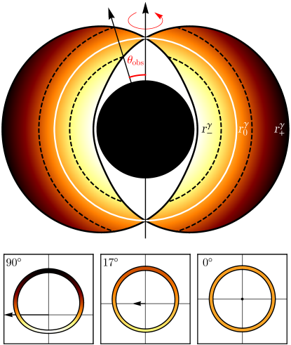
Figure 2: Top: The photon shell of a Kerr black hole with spin $a/M=0.94$. The boundaries $r_{\pm}^{\gamma}$ are shown, as well as the zero-angular-momentum orbit at $r_{0}^{\gamma}=r_{3}$. An observer at $\theta_{\rm o}=17^{\circ}$ only observes the part of the photon ring that corresponds to the intersection of his/her line of sight with the photon sphere. Bottom: The photon ring as viewed by observers at different inclinations. The color matches that of the radii that contribute to the image. Only an observer in the equatorial plane observes the photon ring associated with the entire photon shell. The face-on observer at $\theta_{\rm o}=0^{\circ}$ only observes photons associated with the bound orbit at $r_{\rm o}$. The arrow denotes the projection of the spin axis on the plane perpendicular to the line of sight. This is Figure 2 from JohnsonLupsasca2020 , reproduced under the terms of the Creative Commons Attribution 4.0 International License.

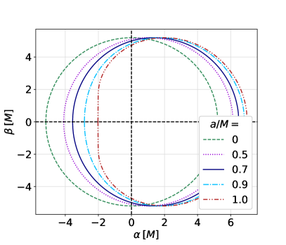
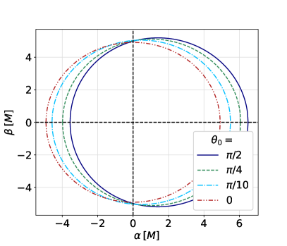
Figure 3: Left: The Kerr critical curve for different values of the black hole spin parameter at an observer inclination $\theta_{\rm o}=90^{\circ}$. Right: The Kerr critical curve for different observer inclinations $\theta_{\rm o}$ in the case of a black hole with spin $a/M=0.7$. The solid curves in both panels correspond to the same critical curve.

0.2.2 Nearly bound orbits, photon rings and critical exponents

The poloidal components (0.2.9)–(0.2.10) of the geodesic equation imply that

$$\pm_{r}\frac{1}{\sqrt{\mathcal{R}(r)}}\frac{dr}{d\sigma}=\frac{E}{\Sigma}=\pm_{\theta}\frac{1}{\sqrt{\Theta(\theta)}}\frac{d\theta}{d\sigma}\,.$$ (0.2.32)

Integrating this equation along a geodesic from affine parameter $\sigma=\sigma_{i}$ to $\sigma=\sigma_{f}$ –corresponding to coordinates $(t_{i},r_{i},\theta_{i},\phi_{i})$ and $(t_{f},r_{f},\theta_{f},\phi_{f})$, respectively—yields

$$\fint_{r_{i}}^{r_{f}}\frac{\mathop{}\!\mathrm{d}r}{\pm_{r}\sqrt{\mathcal{R}(r)}}=\fint_{\theta_{i}}^{\theta_{f}}\frac{\mathop{}\!\mathrm{d}\theta}{\pm_{\theta}\sqrt{\Theta(\theta)}}\,,$$ (0.2.33)

where the slash through each integral indicates that it is to be evaluated along the photon trajectory, with the signs $\pm_{r}$ and $\pm_{\theta}$ chosen to ensure that each integral grows monotonically along the path. These integrals can be reduced to Legendre normal form, that is, they are expressible in terms of three standard elliptic integrals GrallaLupsasca2020b (see also, e.g., Rauch1994 ; Vazquez2004 ; Li2005 ).

We now focus on bound photon orbits with polar turning points (0.2.31) and let $G_{\theta}$ denote the polar integral over one oscillation from $\theta_{-}$ to $\theta_{+}$ (a half period),

$$G_{\theta}\equiv\int_{\theta_{+}}^{\theta_{+}}\frac{\mathop{}\!\mathrm{d}\theta}{\sqrt{\Theta(\theta)}}=2\int_{\pi/2}^{\theta_{+}}\frac{\mathop{}\!\mathrm{d}\theta}{\sqrt{\Theta(\theta)}}\,,$$ (0.2.34)

where the last line follows from the fact that $\theta_{+}=\pi-\theta_{-}$, with the polar oscillation symmetric about the equatorial plane. Using Eq. (0.2.22), we can rewrite this as

$$G_{\theta}=\frac{1}{\sqrt{a^{2}}}\int_{0}^{u_{+}}\frac{\mathop{}\!\mathrm{d}u}{\sqrt{u\left(u_{+}-u\right)\left(u-u_{-}\right)}}=\frac{2}{\sqrt{-a^{2}u_{-}}}K\!\left(\frac{u_{+}}{u_{-}}\right)\,,$$ (0.2.35)

where we introduced the complete elliptic integral of the first kind,

$$K(m)\equiv\int_{0}^{1}\frac{\mathop{}\!\mathrm{d}t}{\sqrt{\left(1-t^{2}\right)\left(1-m\,t^{2}\right)}}\,.$$ (0.2.36)

By construction, $G_{\theta}>0$ represents the polar integral along a complete half-orbit from $\theta_{\pm}$ to $\theta_{\mp}$.

Nearly bound photons

Consider now a photon that is bound at orbital radius $r=\tilde{r}$ within the photon shell $r^{\gamma}_{-}\leq\tilde{r}\leq r^{\gamma}_{+}$, with conserved quantities (0.2.27). If we give it a slight displacement $\delta r_{0}$, such that its initial radius is

$$r_{i}=\tilde{r}+\delta r_{0}\,,\qquad 0<\delta r_{0}\ll\tilde{r}\,,$$ (0.2.37)

then the photon becomes unbound. As long as the photon remains near its orbital shell, its radial potential can be approximated as

$$\mathcal{R}(r)\approx\frac{1}{2}\mathcal{R}^{\prime\prime}(\tilde{r})\left(\delta r_{0}\right)^{2}\,,$$ (0.2.38)

since $\mathcal{R}(\tilde{r})=\mathcal{R}^{\prime}(\tilde{r})=0$ by Eq. (0.2.26) applied to the bound orbit at radius $\tilde{r}$. For simplicity, we suppose that the photon starts in the equatorial plane at $\theta_{i}=\pi/2$. After completing $n$ polar half-orbits between $\theta_{\pm}$ and $\theta_{\mp}$, the photon has moved to a radius $r_{f}=\tilde{r}+\delta r_{n}$ that is determined by the poloidal geodesic equation (0.2.33),

$$\int_{\tilde{r}+\delta r_{0}}^{\tilde{r}+\delta r_{n}}\frac{\mathop{}\!\mathrm{d}r}{\sqrt{\mathcal{R}(r)}}=nG_{\theta}(\tilde{r})\,.$$ (0.2.39)

Using (0.2.38), the radial integral can be approximated as

$$\int_{\tilde{r}+\delta r_{0}}^{\tilde{r}+\delta r_{n}}\frac{\mathop{}\!\mathrm{d}r}{\sqrt{\mathcal{R}(r)}} \approx\int_{\tilde{r}+\delta r_{0}}^{\tilde{r}+\delta r_{n}}\frac{\mathop{}\!\mathrm{d}r}{\sqrt{\frac{1}{2}\mathcal{R}^{\prime\prime}(\tilde{r})(r-\tilde{r})^{2}}}=\sqrt{\frac{2}{\mathcal{R}^{\prime\prime}(\tilde{r})}}\ln\left(\frac{\delta r_{n}}{\delta r_{0}}\right)\,.$$ (0.2.40)

Hence, the radial deviation $\delta r=r-\tilde{r}$ of the photon from its nearby bound orbit grows exponentially (as long as $\delta r$ is small). This exponential instability, which is characteristic of unstable fixed points, may be quantified by the Lyapunov exponent

$$\gamma\equiv\sqrt{\frac{\mathcal{R}^{\prime\prime}(\tilde{r})}{2}}G_{\theta}(\tilde{r})\,,$$ (0.2.41)

which controls the exponential rate of radial deviation,

$$\delta r_{n}=e^{\gamma n}\delta r_{0}\,.$$ (0.2.42)

Using the expressions (0.2.14), (0.2.27), and (0.2.35), we obtain an explicit expression for the Lyapunov exponent of Kerr photon orbits,

$$\boxed{\gamma(r)=\frac{4}{\sqrt{-a^{2}u_{-}}}\sqrt{r^{2}-\frac{Mr\Delta}{(r-M)^{2}}}K\!\left(\frac{u_{+}}{u_{-}}\right)\,.}$$ (0.2.43)

This Lyapunov exponent is a function of the black hole mass $M$, its spin $a$, and the photon orbital radius $r$. At every such radius, we can invert $\phi_{R}(r)$ from Eq. (0.2.18) to obtain the orbital radius $r(\phi_{R})$ corresponding to polar angle $\phi_{R}$ around the critical curve. Thus, we may also regard the Lyapunov exponent as a function $\gamma(\phi_{R})$ of the polar angle around the observer screen. This is illustrated in Figure 4.

As described in our earlier discussion, off-equatorial observers only probe a subset of the bound orbits in the photon shell $r_{-}^{\gamma}\leq r\leq r_{+}^{\gamma}$. As a result, it follows that the function $\gamma(\phi_{R})$ computed for an equatorial observer contains all the information encoded in $\gamma(\phi_{R})$ computed for off-equatorial observers (but the converse is not true). The angles $\phi_{R}^{\pm}$ between which an equatorial observer probes the radii observable from inclination $\theta_{\rm o}$ obey the approximate relation Staelens2023

$$\phi_{R}^{\pm}\approx\left(\frac{\pi}{2}\pm\theta_{\rm o}\right)\mod\pi\,.$$ (0.2.44)

Figure 4 illustrates this for an observer at inclination $\theta_{\rm o}=17^{\circ}$, for whom $\phi_{R}^{-}\approx 73^{\circ}$ and $\phi_{R}^{+}\approx 107^{\circ}$.

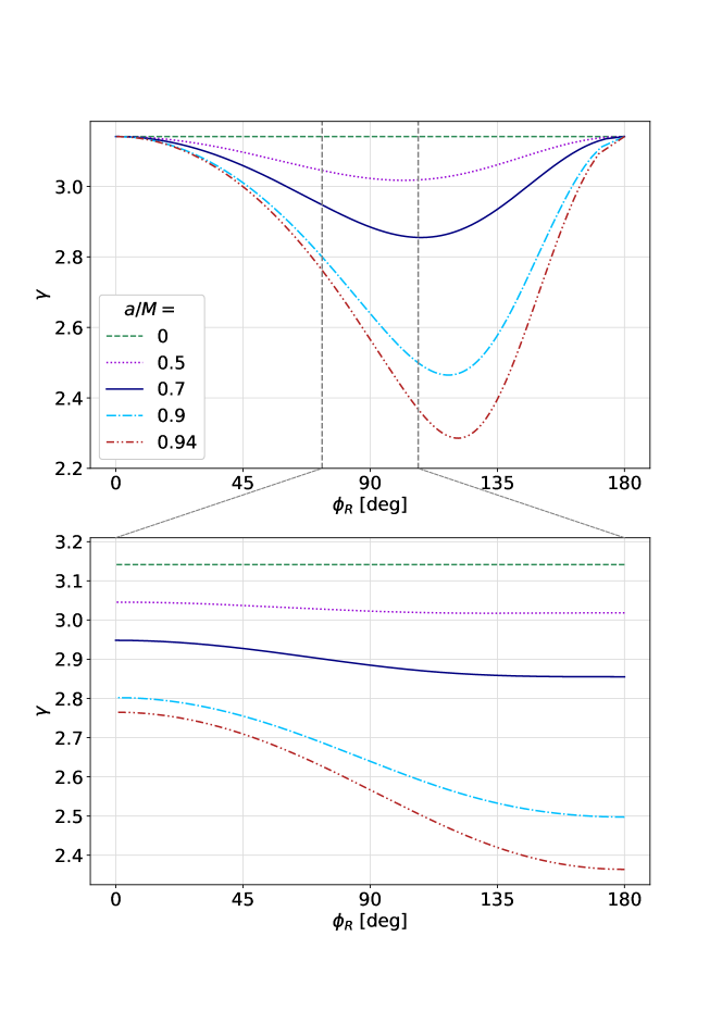
Figure 4: The Lyapunov exponent $\gamma$ as function of the polar angle $\phi_{R}$ around the observer screen, for different values of the spin parameter $a/M$ in the Kerr metric. The function $\gamma(\phi_{R})$ accessible to an observer at inclination $\theta_{\rm o}=17^{\circ}$ (bottom) is a subset of the full range accessible to an equatorial observer (top).

.

The photon ring

The existence of nearly bound photon orbits is responsible for the appearance of a striking and universal feature in black hole images: the photon ring Beckwith2005 ; Gralla2019 ; JohnsonLupsasca2020 . This bright, narrow ring arises from light rays that are strongly bent by the gravitational pull of the black hole and orbit through its surrounding emission multiple times—collecting additional photons in each pass through the emission—before reaching the observer and producing a brightness enhancement close to the critical curve.

Consider a point with coordinates $(R_{c},\phi_{R})$ on the critical curve. A light ray that is aimed outside the critical curve at a small perpendicular distance $\delta R_{n}>0$ from this point will typically cross the equatorial plane a number of times of order JohnsonLupsasca2020

$$n\approx-\frac{1}{\gamma(\phi_{R})}\ln\left(\frac{\delta R_{n}}{R_{c}}\right)\,.$$ (0.2.45)

It follows that for this light ray to complete an additional half-orbit around the black hole, it must be aimed exponentially closer to the critical curve, at a distance

$$\delta R_{n+1}\approx e^{-\gamma(\phi_{R})n}\delta R_{n}\,.$$ (0.2.46)

The photon ring then consists of an infinite series of subrings, such that the $n^{\text{th}}$ subring contains photons that completed a fixed number $n$ of equatorial crossings on their way from source to observer. As described by Eq. (0.2.46), the Lyapunov exponent governs how each successive subring grows exponentially closer to the critical curve and moreover decreases exponentially in width. For a Schwarzschild black hole, this phenomenon was first understood by Darwin Darwin1959 and numerically investigated by Luminet Luminet1979 .

The photon ring is an important and ubiquitous feature in black hole images. The photon subrings’ precise locations on the observer screen depend on the emission responsible for them, although the $n^{\text{th}}$ subring will always lie in a well-defined $n^{\text{th}}$ “lensing band”: a region of the observer screen consisting of all the possible light rays that could achieve at least $n$ half-orbits around the black hole on their trajectory Paugnat2022 ; CardenasAvendano2023 . If the black hole is surrounded by an optically thin equatorial disk emitting photons isotropically, then a geodesic that crosses the equatorial plane (and therefore also the accretion disk) $n$ times will contain $\sim n$ times more photons compared to a geodesic that only crosses the disk once. Therefore, the intensity of rays lying in high-$n$ photon subrings is expected to be larger by a factor $\sim n$ as well Gralla2019 ; JohnsonLupsasca2020 . We will discuss the interferometric signatures of the photon ring in Section 0.3.2 and some more of its observable features in Sections 0.3.3, 0.3.4, and 0.3.5.

Critical exponents of the photon shell and ring

We complete the discussion of (nearly) bound geodesics and the photon ring by describing the two critical exponents $\delta$ and $\tau$ that characterize the toroidal motion of bound photons.

Following GrallaLupsasca2020a (see also Teo2003 ), we can integrate the geodesic equations (0.2.11) and (0.2.12) for $\phi$ and $t$ along a geodesic bound at a fixed orbital radius $r$ to obtain:

$$\Delta\phi=a\left(\frac{r+M}{r-M}\right)\int\frac{\mathop{}\!\mathrm{d}\theta}{\pm_{\theta}\sqrt{\Theta(\theta)}}+\lambda\int\frac{\csc^{2}{\theta}}{\pm_{\theta}\sqrt{\Theta(\theta)}}\mathop{}\!\mathrm{d}\theta\,.$$ (0.2.47)

Over a complete half-orbit ($\theta_{\pm}$ to $\theta_{\mp}$), this change in $\phi$ can be denoted by $\hat{\delta}$. However, $\hat{\delta}$ is not a smooth function of the bound orbit radius $r$, as it has a $2\pi$ jump discontinuity at the pole-crossing bound orbit $r_{\rm o}$ for which $\lambda=0$ Teo2003 ; GrallaLupsasca2020a . It is therefore more natural to define a smooth function $\delta=\hat{\delta}+2\pi H(r-r_{\rm o})$, or more explicitly,

$$\delta=2a\left(\frac{r+M}{r-M}\right)G_{\theta}+\lambda\int_{\theta_{-}}^{\theta_{+}}\frac{\csc^{2}{\theta}}{\sqrt{\Theta(\theta)}}\mathop{}\!\mathrm{d}\theta+2\pi H(r-r_{\rm o})\,,$$ (0.2.48)

where we used the Heaviside step function $H(x)$, and $G_{\theta}$ defined in (0.2.35). This expression defines the critical exponent $\delta$ for Kerr; by definition, it determines the $\phi$ motion of the bound orbit at radius $r$ (and nearly bound geodesics at radii $r+\delta r$).

In an entirely similar way (although without the complication involving the pole-crossing orbit $r_{\rm o}$), we can convert the $t$ integral coming from (0.2.12) to an angular integral over $\theta$; the resulting integral over one complete half-orbit defines the critical exponent $\tau$:

$$\tau=2r^{2}\left(\frac{r+3M}{r-M}\right)G_{\theta}+a^{2}\int_{\theta_{-}}^{\theta_{+}}\frac{\cos^{2}{\theta}}{\sqrt{\Theta(\theta)}}\mathop{}\!\mathrm{d}\theta\,.$$ (0.2.49)

These expressions for $\delta$ and $\tau$ can be written in terms of elliptic integrals GrallaLupsasca2020a . The critical exponents $\gamma$, $\delta$, and $\tau$ control black hole lensing GrallaLupsasca2020a and play a crucial role in the description of photon ring brightness autocorrelations Hadar2021 ; see Section 0.3.5.

Extension to other spacetimes

In this Section (and in Section 0.2.1), we have focused on the calculation of bound null orbits, the critical curve, and the critical exponents $\gamma$, $\delta$, and $\tau$ governing the (nearly) bound geodesics that make up the photon rings of Kerr black holes. All of these calculations can be extended to other black hole metrics, as long as they admit a separable null geodesic equation (and thus a fourth, Carter-like conserved quantity); see Staelens2022 ; Staelens2023 ; Wielgus2021 ; Ayzenberg2022 ; Omwoyo2023 ; Olmo2023 for some examples.

In spacetimes where the null geodesic equation is not separable, bound photon orbits will generically still exist, although it is perhaps not clear how a critical curve can be defined unambiguously (see Staelens2023 for an example). Recently, a formalism for calculating Lyapunov exponents in spacetimes with non-separable geodesics was developed in Deich2023 , which exploits the definition of the Lyapunov exponent as the measure of instability along the trajectory of a bound orbit in geodesic phase space.

0.2.3 Interferometric black hole imaging

The Event Horizon Telescope (EHT) images black holes using a technique known as Very-Long-Baseline Interferometry (VLBI). That is, it is a radio interferometer composed of antennas located at the different telescope sites in the array. Each of these antennas measures a local electric field as a function of time $t$, frequency $\nu$, and polarization $P$; we can then consider the complex cross-correlation between the measured electric field for each pair of antennas $(i,j)$, a quantity known as the interferometric visibility:

$$V_{ij}(t,\nu,P_{1},P_{2})=\left\langle E_{i}(t,\nu,P_{1})E_{j}^{*}(t,\nu,P_{2})\right\rangle\,.$$ (0.2.50)

There are four possible such cross-correlations, corresponding to the four different combinations of polarization $(P_{1},P_{2})$. We will focus here on the total (brightness) intensity of the image, which corresponds to one particular combination of these correlations Roberts1994 (see Section 0.3.3 for a discussion of the observed polarization, which corresponds to a different cross-correlation).

Every pair of antennas in the array thus samples the complex visibility $V$, which is related by the van Cittert-Zernike theorem vanCittert1934 ; Zernike1938 to the Fourier transform of the image brightness $I$ in the plane of the sky: if $\mathbf{x}=(x,y)$ are dimensionless Cartesian coordinates in the image plane (measured, for instance, in radians), then

$$V(\mathbf{u})=\int I(\mathbf{x})e^{-2\pi i\mathbf{u}\cdot\mathbf{x}}\mathop{}\!\mathrm{d}^{2}\mathbf{x}\,,$$ (0.2.51)

where the dimensionless “baseline” $\mathbf{u}$ can be viewed as a vector projected onto the plane perpendicular to the line of sight to the source, and measured in units of the observation wavelength $\lambda=c/\nu$. Each baseline $\mathbf{u}$ joining two antennas in the interferometric array samples a complex visibility $V(\mathbf{u})$, which corresponds to a single Fourier component of the sky image $I(\mathbf{x})$. Technical and environmental limitations make the phase of the visibility difficult to measure; on the other hand, it is comparably easier to access the visibility amplitude $|V|$ (sometimes also called the “visamp”). More details on interferometry can be found in Roberts1994 ; EHT2019IV , for instance.

Each pair of antennas only measures the visibility $V$ at a given baseline $\mathbf{u}$ (which changes somewhat over time due to the rotation of the Earth); see Figure 5. We clearly never have access to the entire visibility function $V(\mathbf{u})$: this means that, even in principle, we do not have enough information to completely reconstruct the image brightness $I(\mathbf{x})$ from its sparsely sampled Fourier transform. Therefore, any “image” produced from EHT observations necessarily relies on assumptions and modeling. This point is well-illustrated by the first four “images” produced independently by the four imaging teams within the EHT collaboration from the first observations of M87 (see Figure 6): the same sparse interferometric data is consistent with a wide range of reconstructed images EHT2019IV . Only the features that are consistent across all images (reconstructed via different algorithms) should be treated as robust; other features are likely artifacts of a particular reconstruction method.

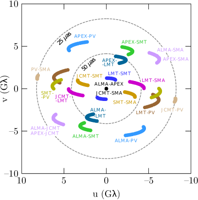
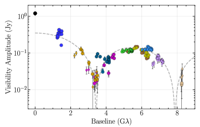
Figure 5: Left: Plot of the visibility points in the baseline plane $\mathbf{u}=(u,v)$ sampled by the different pairs of telescopes in the EHT array in its 2017 observations of M87. The tracks are produced by the Earth’s rotation, which helps fill out the baseline plane (this is known as “Earth rotation aperture synthesis”). Right: The corresponding measured visibility amplitudes (overlaid with a Fourier transform of a symmetric thin ring model, display as a dashed line). This is Figure 2 of EHT2019I .

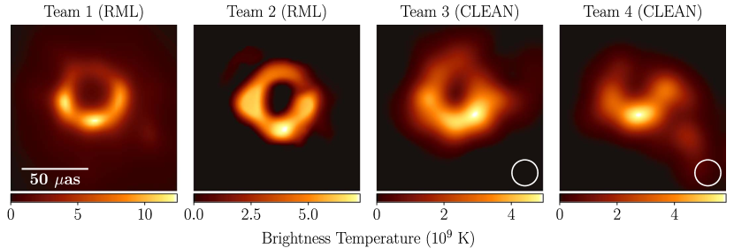
Figure 6: Four different images reconstructed by independent EHT imaging teams from the sparsely sampled interferometric data collected in the 2017 EHT observations of M87. Each image was produced by a different image reconstruction algorithm (named above its panel). This is Figure 4 of EHT2019IV , where these different algorithms are described.

In addition to the image uncertainty due to sparse interferometric sampling, there is an additional uncertainty in the physics of the emitting plasma in the accretion flow EHT2019V ; EHT2022V : Figure 7 shows images obtained from simulated EHT observations of three very different emission models for the plasma in the accretion disk. We further discuss this physical uncertainty in Section 0.2.4 below.

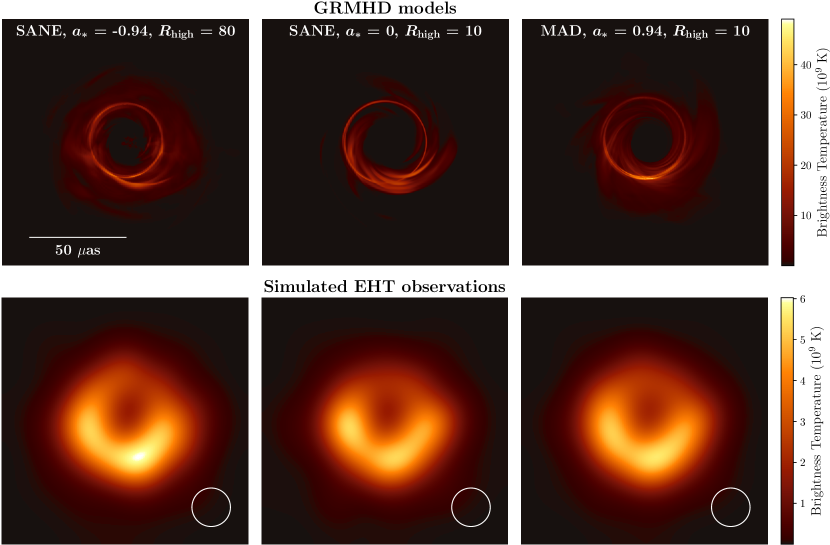
Figure 7: Three snapshots (top) and their corresponding simulated EHT observations (bottom) raytraced from GRMHD simulations with different prescriptions for the electron heating (which is modeled in post-processing and not from first principles). This is Figure 4 of EHT2019I .

It is also important to mention the timescales involved in these observations. In particular, the EHT images of M87^∗ shown in Figures 6 and 7 can be understood as time-averaged images. The EHT observations range over a number of days; since the plasma around the black holes evolves in time, its emission changes during the observation period. The timescale of the plasma dynamics is likely correlated with the black hole’s mass and set by its light-crossing time; for M87^∗, this is roughly $GM/c^{3}\approx 9$ hours, so the effect is still rather mild in the EHT’s multi-day observations of M87^∗ EHT2019I . On the other hand, the black hole at the center of our galaxy, Sgr A^∗, is about 1,500 times lighter than M87^∗; its dynamical timescale is on the order of $GM/c^{3}\approx 21$ seconds. Accordingly, the EHT observations of Sgr A^∗ do indeed show significant variability in the image over its measurement period EHT2022I ; EHT2022IV . This variability makes it more challenging to time-average observational data and leads to larger uncertainties in the reconstructed image compared to M87^∗. At the same time, it could also be an asset for GR tests, as it produces autocorrelations (between fluctuations in the direct image and their light echoes) whose measurement would provide a sharp probe of the underlying geometry—see discussion in Section 0.3.5.

There are clearly many uncertainties in the interferometrically sampled image and the underlying plasma physics. To extract information about the underlying geometry—that is, to access information that can potentially test GR—the relevant question is then: What features of a black hole “image” are universal, i.e., shared by all (or at least, most) interferometric image reconstruction methods as well as physical emission models? Only such universal features can reliably be used to extract robust geometrical data about the black hole geometry and thus lead to potential tests of gravitational physics.

Perhaps the most obvious universal feature of the produced black hole images (see Figures 6 and 7) is the existence of a bright ring-like structure surrounding a dark brightness depression (often called the “shadow”, but see further below in Section 0.3.1). Such a bright ring reveals itself in the actual interferometric signal as a Bessel-function-like behavior of the visibility amplitude (see Figure 5). The presence of a bright ring surrounding a central brightness depression is itself a nontrivial prediction of GR, which certainly indicates the existence of an ultracompact object at the center of the source EHT2019I , and allows for an estimate of this object’s mass EHT2019VI . The asymmetry of the image is also fairly robust and can be attributed to a nonzero spin of the object, although it is harder to make a quantitative estimate of this angular momentum from the image EHT2019V .

Of course, the mass and angular momentum of the central object are only its most basic properties. To really test GR, we need to be able to extract more detailed properties and features of the underlying geometry We will discuss this prospect further in Section 0.3; in particular, we will argue that the most promising method for extracting such geometric properties is from precise interferometric features of the bright ring in the image, that is, from the photon ring.

0.2.4 Plasma physics uncertainties in simulations of the emission

In the Section above, we discussed the interferometric observations that eventually lead to a black hole “image”, and the uncertainties inherent in these observations themselves. Here, we focus on the physics of the source of the measured light: the plasma surrounding the black hole. Clearly, any test of GR using black hole images must be able to disentangle the physics of the emitting plasma from the effects of the underlying geometry, so it is important to highlight the difficulties and unknowns associated with the plasma physics. We also briefly mention a few image simulation techniques and provide some possible starting points for the reader interested in exploring them further.

The photons observed by the EHT are assumed to be mainly emitted via synchrotron radiation by relativistic electrons in the accretion disk (or potentially from the jet region) EHT2019V ; EHT2022V ; Davelaar2023 . The heating mechanism of the electrons in the accretion disk, and hence their temperature (which is essential for modeling their emission), is currently unknown. It is unlikely that a single mechanism is at play everywhere in the accretion disk, and understanding the interplay between the most often conjectured heating mechanisms (such as turbulence, magnetic reconnection, and shocks) requires high-accuracy numerical simulations resolving all key physical processes.

To calculate the temperature and dynamics of radiating electrons, a fully kinetic solution is required; that is, one would have to numerically solve the Vlasov equation in the curved spacetime of the black hole. However, a crucial difficulty in solving the Vlasov equation for the emitting electrons in the accretion disk plasma is that there is a large separation of scales between the size of the black hole and the typical plasma length scales, which are the Larmor radius (the radius of an electron’s gyrating motion in a magnetic field) and the skin depth (the depth to which electromagnetic radiation can penetrate the plasma). For example, for Sgr A^∗ (resp. M87^∗), the gravitational radius is $r_{\rm g}=GM/c^{2}\simeq 6.1\times 10^{11}\,\rm{cm}$ (resp. $r_{\rm g}\simeq 9.1\times 10^{14}\,\rm{cm}$); whereas the nominal Larmor radius $r_{\rm L}\sim m_{e}c^{2}/\left(|e|B_{0}\right)\sim\mathcal{O}(100\,\rm{cm})$, and the skin depth $d_{\rm e}=cm_{\rm e}^{1/2}/\left(4\pi n_{\rm e}e^{2}\right)^{1/2}$ is of similar order as the Larmor radius $\mathcal{O}(500\,\rm{cm})$ for an electron number density $n_{\rm e}\simeq 10^{6}\,\rm{cm}^{-3}$ for Sgr A^∗ EHT2022V , and $\mathcal{O}(3000\,\rm{cm})$ with $n_{\rm e}\simeq 3\times 10^{4}\,\rm{cm}^{-3}$ for M87^∗ EHT2019V . Kinetic simulations cannot resolve the (realistic) separation between these microscopic plasma scales and macroscopic scales at currently feasible numerical resolutions. However, they can achieve the right hierarchy of scales ($r_{\rm g}\gg d_{\rm e}\gg r_{\rm L}$) for magnetized plasmas Levinson2018 ; Parfrey2019 ; Crinquand2020 ; Chen2020 ; Crinquand2022 ; Galishnikova2023a .

The most commonly used alternative to solving the Vlasov equation is to avoid having to resolve the microscopic plasma scales altogether by averaging over the particle distribution function. This approach leads to a set of fluid equations enforcing the conservation of mass, momentum and energy of the plasma. Coupled to the Maxwell equations in curved spacetime, the resulting set of evolution equations is called general-relativistic magnetohydrodynamics (GRMHD).

For typical EHT sources (i.e., low-luminosity active galactic nuclei), the plasma in the accretion disk and the black hole jet is collisionless, meaning that the mean free path to Coulomb collisions between charged particles is larger than the system size (set by the size of the accretion disk); see EHT2019V for M87^∗ and EHT2022V Sgr A^∗. The collisionless nature of the plasma also typically allows particles to accelerate and form a non-thermal energy tail, so that a Maxwell-Boltzmann distribution function does not accurately capture the plasma temperature. Therefore, electrons and ions in the plasma are not typically in thermal equilibrium and one cannot a priori infer the electron temperature directly from the ion temperature. However, the standard (ideal) form of the GRMHD equations assumes collisional plasma in thermal equilibrium; this describes the temperature and dynamics of the (heavier) ions, but results in the main uncertainty in calculating the essential electron temperature to describe the synchrotron radiation.

Despite their inability to capture the kinetic and collisionless plasma effects, GRMHD simulations do capture the global dynamics of the accretion flow and jet launching reasonably well (see, e.g., Porth2019 for a comparison of the most frequently used GRMHD codes). Even in ideal GRMHD, it is computationally challenging to resolve the scales on which energy dissipates and the plasma is heated, which is needed to probe sites where the observed radiation could be powered. Typical GRMHD simulations employ numerical resolutions at which the magnetorotational instability (MRI) is at least minimally resolved Porth2019 —this is assumed to be one of the main drivers of the turbulence in the accretion disk in the standard turbulent accretion scenario, often called “SANE” (for Standard and Normal Evolution). In GRMHD simulations with 1,000 times higher resolution (10 times per direction) than typical EHT simulations, Ripperda2022 showed that features like magnetic reconnection and specific mechanisms driving the turbulence in the accretion disk can be resolved and result in observable radiation Hakobyan2023 ; Zhdankin2023 , while the overall dynamics remains similar to standard lower-resolution simulations.

The source of the plasma in the jet near its launching point just outside the event horizon is also not well understood. GRMHD simulations have produced such jets and can predict their electromagnetic power Porth2019 . Above a certain radius, in the open-field region of the jet, matter can escape the gravitational pull of the black hole and move outwards, whereas below that surface (the “stagnation surface”), the plasma moves towards the event horizon. This creates a vacuum region around the black hole. In low-luminosity sources like M87, electron-positron pair production cascades will maintain a certain density (see, e.g., Levinson2018 ; Crinquand2020 ; Chen2020 ). However, in GRMHD the jet is magnetically insulated from the accretion flow, and as a result matter has to be artificially injected to maintain numerical stability. Therefore, in the vicinity of the event horizon, GRMHD fails completely and a kinetic description is required to model the electron density, temperature, and emission.

Recently, Galishnikova2023a was for the first time able to conduct a general-relativistic kinetic simulation of a simplified (yet relevant for Sgr A^∗; see, e.g., Ressler2020 ) two-dimensional spherically infalling (accreting) plasma, and to compare it to a GRMHD simulation; it was found that there are many similarities in the global flow dynamics despite the differences caused by significant departures from thermal equilibrium (e.g., pressure anisotropies and heat fluxes not captured in GRMHD).

Some kinetic effects can be captured in GRMHD simulations by introducing macroscopic quantities (such as resistivity, viscosity, heat conduction, pressure anisotropies, etc.) or by evolving an additional equation for the electron temperature Bugli2014 ; Ressler2015 ; Chandra2015 ; Foucart2016 ; Chael2017 ; Chandra2017 ; Foucart2017 ; Qian2018 ; Ripperda2019 ; Vourellis2019 ; Ripperda2020 ; Most2021 ; Nathanail2022 ; Most2022 ; Vos2023 . However, such subgrid models require careful benchmarking with kinetic simulations to test their validity (e.g., Bransgrove2021 ). These models typically require additional terms in the GRMHD equations describing the dissipation of energy and magnetic flux occurring on small scales, once again requiring high numerical resolutions to simulate these effects.

In addition to major uncertainties due to collisionless and (underresolved) non-ideal plasma effects, the large-scale plasma flow geometry itself could also vastly differ from what is typically assumed and simulated—it is still unclear what the driver of the accretion is in the centers of galaxies. In the Magnetically Arrested Disk models (“MAD” Igumenshchev2003 ; Narayan2003 , as opposed to the SANE models mentioned above) favored by the EHT observations for both M87^∗ and Sgr A^∗, a large ordered magnetic field forms near the event horizon. In this MAD regime, the accretion flow goes through a relatively lengthy turbulent phase, increasing magnetic flux on the event horizon until the flux gets expelled quickly in a large eruption, after which the magnetic field forms a barrier that transiently halts the accretion BisnovatyiKogan1974 ; BisnovatyiKogan1976 ; Narayan2003 . These flux eruptions are thought to play an essential role in the dynamics and geometry of the accretion flow Chatterjee2022 . The flux eruptions may also have distinctive signatures in the EHT image Jia2023 ; NajafiZiyazi2023 and the photon ring Gelles2022 ; counter-intuitively, they may even dim the image if the inner region emits predominantly at higher energies during an eruption.

All of the simulations mentioned above are initialized using artificial initial conditions, assuming a torus of weakly magnetized matter that becomes unstable and accretes onto the black hole. In particular, the poloidal ($r,\theta$) magnetic field geometry and strength is tuned to obtain either the MAD or SANE scenario described above, whereas more realistic initial conditions are unknown and under-explored.

It is for example unclear whether the strong field that is required to reach the MAD regime and launch a jet grows through a dynamo Liska2020 ; JacqueminIde2023 or is provided by the larger-scale environment. For example, the accretion flow onto Sgr A^∗ is thought to be fed by stellar winds from the galactic center. Depending on the properties of the winds, the inner accretion region may become MAD Ressler2020 , but the flow dynamics would differ significantly from the standard MAD simulations, which can have a distinguishable effect on the EHT image and variability Jia2022 ; Murchikova2022 . For supermassive black holes in elliptical galaxies, like M87^∗, pioneering work by Guo2023 showed that the inner accretion flow can significantly differ from the typically assumed MAD and SANE scenarios. One interesting outcome from wind-fed accretion is the possibility of a tilted accretion disk with respect to the black hole spin axis Ressler2023 . The effects of tilted accretion disks on the dynamics of the accretion flow have been explored extensively Chatterjee2020 ; White2020 ; White2022 ; Chatterjee2023 and can also result in distinguishable features in the images of M87^∗ and Sgr A^∗. Recently, another model was proposed by Blandford2022 exploring the possibility that the observed radiation would be produced in dissipative current sheets in an ergomagnetosphere, contrary to the standard MAD or SANE picture. It is clear that the initial conditions used in standard simulations are artificial, and more astrophysically motivated accretion disk models have to be explored with GRMHD simulations to study the dynamics of the flow that leads to the observed emission.

To produce an image, the photon emission from the plasma must be simulated. Typically, the distribution function of the emitting electrons (and hence their temperature) is put in by hand in a post-processing procedure. Based on density, pressure, velocity and magnetic fields from a GRMHD simulation, emission and absorption properties are assigned to the radiating electrons, and a resulting Boltzmann equation for the emitted photons can then be solved. A total intensity image is then produced by numerically ray tracing the photon trajectories in curved spacetime, solving along each ray the radiative transport equations that describe how the photons are emitted, absorbed, and scattered within the plasma. The numerical methods for solving these equations are well-established and well-tested and can in principle be integrated to arbitrary accuracy (see Bacchini2018 ; Gold2020 ; Prather2023 for comprehensive comparisons between ray tracing methods and radiative transfer codes). The main uncertainty in the simulated radiation and resulting image lies in the assumptions used for the electron temperature and its dependence on the GRMHD variables.

GRMHD simulations are computationally expensive, typically requiring on the order of 1 million CPU hours per simulation (depending on resolution and integration time). To find clear effects of the underlying geometry, one would in principle need to simulate many different GRMHD scenarios and identify universal features of the resulting images that are signatures of the geometry and not dependent upon the details of the plasma; see also Gralla2021 ; Lara2021 ; Ozel2022 ; Bauer2022 for more discussion of how to separate plasma effects from geometry. For this reason, it can make sense to shortcut the GRMHD simulation step and instead use emission models that mimic to some extent the effects of GRMHD models, but instead are orders of magnitude less computationally expensive. This can enable the quick simulation of many different emission scenarios and help identify such universal signatures of the underlying geometry.

One example of an emission-mimicking model is that of an equatorial and optically thin emission disk introduced in GLM2020 (see also CardenasAvendano2022 for a detailed description). Geodesics that pass through the equator “pick up” extra intensity (representing the emission from the disk), resulting in a total brightness $I$ of a geodesic given by:

$$I_{\rm o}=\sum_{n=0}^{N}\xi_{n}\,g^{3}\!\left(r^{(n)}\right)\,I_{\rm s}\!\left(r^{(n)},\phi^{(n)},t^{(n)}\right)\,,$$ (0.2.52)

where $I_{\rm s}$ is the local source intensity at the position where the light ray crosses the equatorial disk, $(r^{(n)},\phi^{(n)})$ is the location of the $(n+1)^{\text{th}}$ equatorial crossing, which occurs at time $t^{(n)}$, $g$ is the observed redshift (i.e., the relative redshift between the observer and the emitting plasma), $N+1$ is the total amount of times the geodesic crosses the equatorial plane, and $0<\xi_{n}$ is a “geometric fudge factor” that can be adjusted to mimic the effects of absorption or geometrical thickness of the emitting disk GLM2020 ; Chael2021 ; Paugnat2022 ; CardenasAvendano2022 .

A good choice for the local intensity function $I_{s}$ is such that its image (0.2.52) reproduces the main features seen in time-averaged GRMHD images. Such a function, derived from Johnson’s SU distribution, was introduced in GLM2020 ; CardenasAvendano2022 :

$$I_{\rm s}=\frac{e^{-\frac{1}{2}\left[\gamma+\sinh^{-1}\left(\frac{r-\mu}{\sigma}\right)\right]^{2}}}{\sqrt{(r-\mu)^{2}+\sigma^{2}}}\,.$$ (0.2.53)

The tuneable parameters $\gamma$, $\mu$, and $\sigma$ can be used to simulate different types of emission Paugnat2022 . The redshift factor $g$ is determined by a model for the fluid flow in the equatorial disk, which contains further tuneable parameters; see, e.g., CardenasAvendano2022 (especially Appendix B therein) for further details.

Finally, keeping all of the above uncertainties and caveats in mind, we mention a few pedagogical starting points for the reader interested in simulating EHT images.

A commonly employed open-source GRMHD code that the authors are familiar with is the BlackHoleAccretionCode (BHAC) Porth2017 ; Olivares2019 (see Porth2019 for a comprehensive overview of GRMHD codes). BHAC solves the GRMHD equations in arbitrary spacetimes and coordinates, and has been extended to incorporate a non-ideal resistive GRMHD module Ripperda2019 . BHAC has the ability to employ adaptive mesh refinement techniques with an oct-tree block-based approach, to increase the grid resolution in particular regions. The code uses a second-order finite volume method and a constrained transport algorithm to maintain a divergence-free magnetic field Olivares2019 . Typical simulations employ spherical Kerr-Schild coordinates (with $r$, $\theta$, and $\phi$ the radial, poloidal and toroidal angular coordinates, respectively) and use a torus in hydrodynamic equilibrium Fishbone1976 as initial condition. A public release version, including documentation and example setups of MAD and SANE accretion disk scenarios, can be obtained from https://bhac.science.

We also mention two ray tracing codes that the authors are particularly familiar with and which are completely open-source. First of all, the Adaptive Analytic Ray Tracing code AART CardenasAvendano2022 analytically integrates null geodesics in the Kerr geometry and can simulate both the stationary emission model described above around (0.2.52), as well as time-dependent images. The analytic integration method, as well as a nonuniform adaptive grid tailored to the lensing bands of Kerr, make it a very fast and efficient code for simulating properties of photon rings in Kerr (for lensing bands beyond Kerr, see CardenasAvendano2024 ). Another ray tracer that simulates stationary emission (but currently does not support time-dependent emission) is the Flexible Object-Oriented Ray Tracer FOORT FOORT , which numerically integrates null rays in arbitrary geometries. FOORT is especially developed with maximal flexibility in mind, so as to be able to accommodate the study of other metrics, and allows for an easy simulation of images of beyond-GR objects. Both AART and FOORT can further process images to produce simulated visibility amplitudes. They are available at https://github.com/iAART/aart and https://github.com/drmayerson/FOORT.

0.3 Brief overview of possible observables

In this Section, we will review a number of features of black hole images. We will especially emphasize the extent to which these features have been argued to be universal and robust in the sense we discussed above; that is, to what extent each feature is controlled by the underlying geometry and whether or not it critically depends on the (unknown) details of the plasma emission.

0.3.1 Black hole shadow and critical curve

In the literature on black hole imaging (especially that which is focused on extracting geometrical data from such observations, or testing GR), the term “shadow” is used both ubiquitously and ambiguously. Here, we attempt to give an overview of the possible definitions of the shadow, and its possible observable properties. A pioneering work in the emission-dependence of the “shadow” is by Gralla, Holz, and Wald Gralla2019 (although we deviate somewhat from their original terminology here).

As discussed in Section 0.2.1, geodesics traced backwards from the observer screen towards the black hole can be divided into two categories: those that eventually fall into the black hole and those that escape to infinity in the far past. The boundary separating those regions (which itself is strictly not part of either region) is the critical curve and corresponds to asymptotically bound photon orbits around the black hole. As we reviewed, the critical curve is well-known for Kerr Gralla2020 ; GrallaLupsasca2020c .

A “mathematical shadow” could then be defined as the collection of points on the observer screen that lie inside the critical curve, i.e., those that correspond to geodesics that eventually fall into the black hole when traced backwards far enough. Note that, by definition, the critical curve is an infinitely thin mathematical curve, and is not in itself directly observable: depending on the astrophysical scenario, the emission may or may not produce a brightness deficit that coincides with it.

By contrast, a more physical notion of “image shadow” can be defined as the (generically present) central brightness depression in a black hole image. More precisely, one could specify the “outer shadow” as the region interior to the bright ring appearing in black hole images (a separate feature known as the “inner shadow” Chael2021 will be discussed below). This remains a rather ambiguous definition—for example: where do we consider the bright ring to “end” precisely? In other words, how do we specify the boundary of the outer shadow? This ambiguity only worsens when considering observations with less-than-perfect resolution (as in realistic situations) in which the surrounding (photon) ring is rather blurred.

Clearly, the mathematical shadow (as defined above) is a precise notion, whereas the image shadow is not. It is important to note that the relation between these two notions of shadow depends on the details of the emission. For example, emission coming from “in front” of the black hole will spoil the central brightness depression. Only for very fine-tuned emission models will these two notions of shadow coincide: this can occur, for example, if the accretion flow around the black hole is spherically symmetric and optically thin Falcke2000 ; Narayan2019 . However, in most cases, including those favored by EHT observations, these two notions of shadow will differ. In principle, the discrepancy can be quite large Gralla2019 , though it has been argued that a large class of realistic emission models give (only) a small—yet still measurable—amount of deviation Bronzwaer2021 . In any case, a measurement of the image (outer) shadow does not necessarily imply a measurement of the mathematical shadow or of the critical curve.

There is thus a tension between the notions of critical curve, which defines the mathematical shadow but is a non-observable theoretical construct, and the image feature of the (outer) shadow, which is observable but ambiguous (depends on the details of the emission) and does not necessarily correspond to the critical curve. The outer shadow—and its implicit approximate equivalence with the mathematical shadow—is used in many observational contexts, but one should be careful not to mix the two concepts. For example, the EHT uses the diameter of this central brightness depression as a measure for the mass of the observed black hole EHT2019VI . The analysis of Bronzwaer2021 investigated the image shadow and its (approximate) robustness over many different emission models, providing a partial justification for such measurements using the image shadow for Kerr.

Nevertheless, the critical curve does still play a central role in black hole images. The curve itself is not observable, but the $n^{\text{th}}$ photon subring will converge (exponentially fast in $n$) to the critical curve, which may be viewed as the $n\to\infty$ photon subring (see Section 0.2.2). This means that resolving the diameter of a sufficiently high-$n$ photon subring will give an accurate estimate for the diameter of the critical curve. It seems that in general, the $n=2$ photon subring is already close enough to the critical curve to be virtually indistinguishable from it (at least by eye, though high-resolution space-VLBI observations may still see the difference Paugnat2022 ). In fact, even though the $n\geq 2$ photon rings and the critical curve (the limiting $n\to\infty$ ring) may not exactly coincide, they must follow the same shape GLM2020 ; CardenasAvendano2023 . More precisely, their projected diameter—a notion defined in the Appendix—must follow a specific functional form known as a circlipse (see further discussion in Section 0.3.4). This suggests an alternative pathway (as opposed to the measurement of the image shadow) for using the critical curve to characterize deformations of Kerr: one may quantify deviations from the Kerr prediction for the photon ring shape.

Finally, more recently the notion of (image) “inner shadow” was introduced Chael2021 . It has a precise definition as the direct (weakly lensed) image on the observer screen of the equatorial event horizon. This region, which is illustrated in Figure 8, is markedly smaller than the critical curve or outer shadow. As was argued in Chael2021 , the inner shadow seems to represent a region in the image that is consistently dark across emission models, and thus does represent a universal signature in black hole images that can be measured and compared to the Kerr prediction. However, the dynamic range (i.e., the observable range of brightness intensities) and resolution of the EHT is currently insufficient to resolve this inner shadow brightness depression; the necessary dynamic range could be achieved in the upcoming ngEHT Chael2021 .

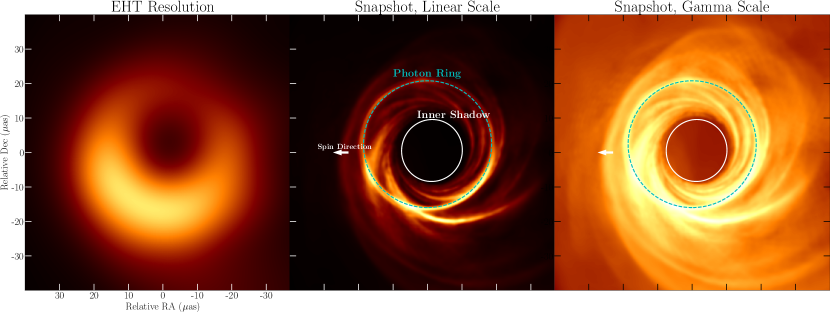
Figure 8: A simulated black hole image. Left: Time-averaged image at EHT resolutions. Middle: A GRMHD snapshot with the photon ring and inner shadow labeled. Right: Same image in a gamma color scale that highlights the central brightness depression. This is Figure 1 of Chael2021 ; further details about the image to be found therein.

0.3.2 Photon ring interferometry

As discussed above, the asymptotically bound photon orbits of Kerr trace out the critical curve on the viewer screen; this is a mathematical construct that is in principle unobservable. By contrast, light rays that follow nearly bound photon orbits can appear on the observer screen very close to the critical curve. Their existence gives rise to an infinite sequence of photon subrings, with each successive ring produced by photons that executed an additional orbit around the black hole on their way from source to observer. Assuming equatorial emission from an optically thin disk, the $n^{\text{th}}$ subring is formed by photons that crossed the equatorial plane $n$ times and thus collected $\sim n$ photons from the emission region (see also Section 0.2.2 above).

The photon rings are not only sharp features in the black hole image; they also produce distinctive interferometric signatures, which were first described in JohnsonLupsasca2020 . Therein, it was argued that for “large enough” $n$, GR predicts that the subring flux ratio of successive subrings must be

$$\frac{F^{n+1}_{\text{ring}}}{F^{n}_{\text{ring}}}\approx e^{-\gamma}\,,$$ (0.3.1)

where $\gamma$ is the Lyapunov exponent (see Section 0.2.2). This statement essentially follows from the fact that successive images are demagnified by $e^{-\gamma}$, and it holds independently of the details of the actual emission. Figure 9 illustrates how the photon ring decomposes into its characteristic subring structure, composed of a sequence of increasingly narrow and tall peaks (the successive photon rings).

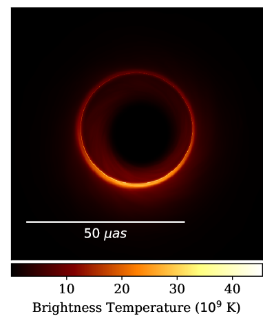
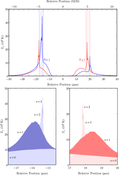
Figure 9: A simulated black hole image (left), and a cross-section of its intensity profile in which individual photon subring intensity peaks are clearly visible for $n=0,1,2,3$ (right). These are Figures 1 and 3 of JohnsonLupsasca2020 , reproduced under the terms of the CC Attribution 4.0 International License.

An important insight of JohnsonLupsasca2020 is that this photon ring brightness profile gives rise to a universal behavior of the complex visibility $V(\mathbf{u})$ on long baselines. In general, a ring with diameter $d$ and thickness $w\ll d$ contributes differently in two (asymptotic) regimes in the visibility JohnsonLupsasca2020 :

$$\textbf{(I):}\quad\frac{1}{d}\ll u\ll\frac{1}{w}\,,\qquad\textbf{(II):}\quad\frac{1}{d}\ll\frac{1}{w}\ll u\,.$$ (0.3.2)

Baselines in regime (I) resolve the diameter of the ring but not its thickness, so that the visibility in this regime behaves as if the ring is a (perfectly) thin ring, displaying damped periodic oscillations with weakly decaying envelope $|V(u)|\sim u^{-1/2}$ (see Section 0.3.4 below for the precise expected form of $V(\mathbf{u})$ in this regime). On the (much) longer baselines of regime (II), both diameter and thickness are resolved, and the visibility is sensitive to the radial profile of the ring; in general, the visibility of a smooth ring in this regime (II) will decay exponentially, as the ring is “resolved out” JohnsonLupsasca2020 . The width-to-diameter ratio for the $n=1$ subring is typically $w/d\lesssim 10\%$, and becomes exponentially smaller by $e^{-\gamma}\approx 5-10\%$ for higher-order subrings.

The $n^{\text{th}}$ photon subring will then dominate the visibility signal in the regime:

$$\frac{1}{w_{n-1}}\ll u\ll\frac{1}{w_{n}}.$$ (0.3.3)

Taken together, the subrings produce in the visibility a cascade of damped oscillations on progressively longer baselines, with each step in the cascade growing exponentially according to the Lyapunov exponent (since the widths of the subrings decrease as $w_{n+1}\approx e^{-\gamma n}w_{1}$). Within each regime (0.3.3), the visibility is dominated by a single subring and carries precise information about its diameter and thickness. This is illustrated in Figure 10, which displays a sample visibility amplitude along with its different subring-dominated baseline regimes.

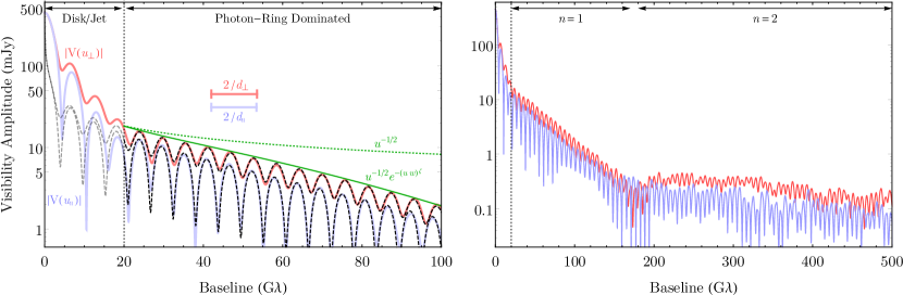
Figure 10: The visibility amplitude corresponding to the image in Figure 9, for baselines perpendicular (red) and parallel (blue) to the black hole spin axis. Left: The universal photon-ring signature begins to dominate the visibility on long baselines. Right: On even longer baselines, the signal from the $n=1$ is taken over by that of the $n=2$ subring. This is Figure 4 of JohnsonLupsasca2020 , reproduced under the terms of the CC Attribution 4.0 International License.

Of course, the universal signatures of the photon subrings were stated above to hold for “large enough” $n$. How big $n$ must precisely be to give a robust, emission-independent observable is unfortunately not entirely clear, and may depend somewhat on the precise photon ring feature being studied. For example, for the photon ring shape discussed below in Section 0.3.4, it has been comprehensively argued over a large range of emission models that $n=2$ is certainly “large enough” to extract universal data GLM2020 ; even the $n=1$ subring seems to be relatively robust over different models CardenasAvendano2023 .

For a given photon ring observable, a careful analysis over many different emission models should be performed before concluding that a given $n^{\text{th}}$ subring gives “universal” results. Existing analyses seem to suggest that $n\gtrsim 2$ and possibly even $n\sim 1$ should be high enough to extract interesting features from the photon ring. This is at least promising from an observational perspective, since only the $n=1$ (and possibly $n=2$) subrings will potentially be resolved with near-future VLBI observations.

0.3.3 Photon ring polarization

The preceding discussion in Section 0.3.2 focused on the observed intensity $I$, which constitutes only one of the electric field correlators that an interferometer measures (see Section 0.2.3). The other cross-correlation functions of the electric field turn out to sample the Fourier transforms of the polarization Stokes parameters Roberts1994 , usually denoted $Q$, $U$ (the linear polarization components), and $V$ (the circular polarization). Similarly to the intensity $I$, these polarimetric quantities display certain universal properties within the photon ring, which were first derived in Himwich2020 .

The linear polarization of light, which was introduced around (0.2.19), is encoded in the Stokes parameters $Q$ and $U$ as follows. Define a two-dimensional vector $\vec{\mathcal{E}}$ on the screen with coordinates $(\alpha,\beta)$ of an observer at inclination $\theta_{\rm o}$ as:

$$\vec{\mathcal{E}}=\left(\mathcal{E}_{\alpha},\mathcal{E}_{\beta}\right)=\frac{\left(\beta\kappa_{2}-\nu\kappa_{1},\beta\kappa_{1}+\nu\kappa_{2}\right)}{\sqrt{\left(\kappa_{1}^{2}+\kappa_{2}^{2}\right)\left(\beta^{2}+\nu^{2}\right)}}\,,\qquad\nu=-\left(\alpha+a\sin\theta_{\rm o}\right)\,,$$ (0.3.4)

where we used the complex Penrose-Walker constant $\kappa$ of (0.2.19). Then the observed parameters $Q$ and $U$ combine into the complex polarization $P$ as

$$P=Q+iU=mIe^{2i\chi}\,,\qquad\chi=\tan^{-1}\left(-\frac{\mathcal{E}_{\alpha}}{\mathcal{E}_{\beta}}\right)\,,$$ (0.3.5)

with $I$ the (Stokes parameter) intensity and $m$ the degree of polarization Himwich2020 . The electric field vector $\vec{\mathcal{E}}$ encodes the direction of polarization of light; its sign is clearly unobservable and thus unphysical. The polarization naturally decomposes into Himwich2020

$$P=(\beta+i\nu)^{2}\mathcal{P}\,,\qquad\mathcal{P}=\left(\frac{mI}{\beta^{2}+\nu^{2}}\right)\frac{\overline{\kappa}}{\kappa}\,,$$ (0.3.6)

which leads to a remarkably simple universal pattern of the polarization within the photon ring. The even subrings (resp. odd subrings) have equal linear polarization $\vec{\mathcal{E}}_{n+2}=\vec{\mathcal{E}}_{n}$, which implies that

$$\mathcal{P}_{n+2}(d_{n+2},\varphi)=\mathcal{P}_{n}(d_{n},\varphi)\,,$$ (0.3.7)

where we expressed $\mathcal{P}=\mathcal{P}(\rho,\varphi)$ as a function of the polar coordinates $(\rho,\varphi)$ on the observer screen, and $d_{n}$ is the radius of the $n^{\text{th}}$ subring (at angle $\varphi$). Moreover, the polarization gets complex-conjugated between odd and even subrings:

$$\mathcal{P}_{n+1}(d_{n+1},\varphi)=\overline{\mathcal{P}}_{n}(d_{n},\varphi).$$ (0.3.8)

The striking universal polarization pattern of the photon ring is a stringent prediction of GR that can in principle be tested. However, as in the discussion of Section 0.3.2, to accurately measure the $n^{\text{th}}$ subring’s polarization, it is necessary to observe the source on very long baselines (0.3.3) dominated by the interferometric signature of the $n^{\text{th}}$ subring. This implies that near-future observations will most likely only be able to measure the polarization of the $n=1$ (and possibly $n=2$) subrings, leaving tests of (0.3.7) beyond reach but perhaps opening the door to tests of (0.3.8). Encouragingly, recent simulations Palumbo2022 suggest that (0.3.8), which was derived in the regime of “large” $n$, may even hold for the direct $n=0$ image and $n=1$ ring. If so, then measuring this characteristic flip in the complex polarization could even lead to the first photon ring detection, before reaching the baselines needed to resolve it Palumbo2023 .

0.3.4 Photon ring shape

In Section 0.3.2, we described how the $n^{\text{th}}$ subring dominates the interferometric visibility within the baseline window (0.3.3), namely over baseline lengths $u$ in the regime

$$\frac{1}{w_{n-1}}\ll u\ll\frac{1}{w_{n}}\,.$$ (0.3.9)

On such baselines, the $n^{\text{th}}$ ring can be approximated by a bright thin curve. Using this insight, Gralla Gralla2020 showed that the visibility amplitude on long baselines (0.3.9) takes the universal form

$$\left|V(u,\varphi)\right|\approx\sqrt{\frac{\left(\alpha_{\varphi}^{\rm L}\right)^{2}+\left(\alpha_{\varphi}^{\rm R}\right)^{2}+2\alpha_{\varphi}^{\rm L}\alpha_{\varphi}^{\rm R}\sin\left(2\pi d_{\varphi}u\right)}{u}},$$ (0.3.10)

where $d_{\varphi}$ is the projected diameter of the curve, illustrated in Figure 11 and precisely defined in the Appendix, while the coefficients $\alpha_{\varphi}^{\rm L,R}$ depend on the intensity profile around the curve.

Measuring the visibility amplitude on sufficiently large baselines and at different angles $\varphi$ in the baseline plane will enable the extraction of the projected diameter $d_{\varphi}$ as a function of polar angle $\phi_{R}=\varphi$ in the image—in other words, a measurement of the shape of the $n^{\text{th}}$ photon ring.

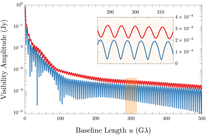
Figure 11: A simulation of the visibility amplitude at $\varphi=0^{\circ}$ (red) and $\varphi=90^{\circ}$ (blue) on long baselines corresponding to the black hole image in Figure 12. The inset displays the clear periodic ringing of (0.3.10) in the long-baseline regime (0.3.9) where the $n=2$ subring dominates. This is part of Figure 4 from GLM2020 .

The shape of the critical curve for the Kerr geometry was investigated in detail in GrallaLupsasca2020c , where it was found that the projected diameter as a function of $\varphi$ is very well approximated by

$$\frac{d_{\varphi}^{\rm circlipse}}{2}=R_{\rm o}+\sqrt{R_{1}^{2}\cos^{2}{\varphi}+R_{2}^{2}\sin^{2}{\varphi}},$$ (0.3.11)

This is called the “circlipse” function as it is the sum of the diameter of a circle, $2R_{\rm o}$, with the diameter of an ellipse with axes $R_{1}$ and $R_{2}$.

Since the photon subrings approach the critical curve at large $n$, it is reasonable to assume that for $n$ “sufficiently” large, the shape of the photon subrings will also be well-described by the circlipse. This was the main argument of Gralla, Lupsasca, and Marrone GLM2020 , who showed that the $n=2$ subring shape (as extracted from mock interferometric data simulated from a wide range of models) can be expected to conform to the circlipse shape to a precision of $\lesssim 0.04\%$ (see Figure 12). This was confirmed by subsequent studies Paugnat2022 ; CardenasAvendano2022 . More recently, it was shown that even a measurement of the $n=1$ subring shape would result in a circlipse, up to errors of order of a percent CardenasAvendano2023 .

In practice, it is technically challenging to extract the ring diameter $d_{\varphi}$ at different angles from (mock) interferometric data and find the best-fit circlipse function. Such a fitting procedure was first developed in GLM2020 and later refined in Paugnat2022 , which provides a comprehensive and detailed explanation of an improved procedure and its complications. To measure the $n=2$ ring and extract its projected diameter, it may be necessary to observe on baselines so large that a distant-Earth orbit mission would be required GLM2020 . By contrast, the $n=1$ subring is already observable on relatively shorter baselines, and so is more likely to be observed in the near-future Gurvits2022 ; Kurczynski2022 ; CardenasAvendano2023 .

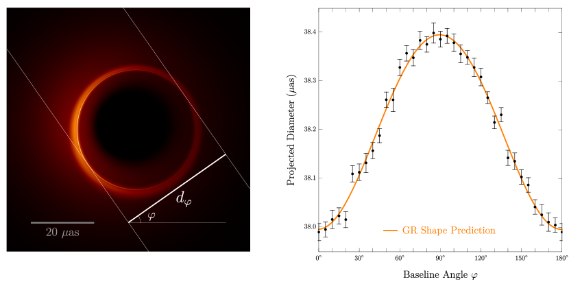
Figure 12: A simulated image of an equatorial disk around a Kerr black hole with spin $a/M=94\%$ viewed at inclination $\theta_{\rm o}=17^{\circ}$ (left), and the projected diameter extracted from the interferometric signature of $n=2$ photon ring at various values $\varphi$ around the baseline plane (right), with the best-fit circlipse shape (0.3.11) shown in orange. This is Figure 1 from GLM2020 .

0.3.5 Photon ring autocorrelations

The light-emitting plasma around the black hole is expected to be a complex, turbulent medium, far from equilibrium. As such, the emission that sources the photon rings will be subject to (brightness) fluctuations. Different photons produced by the same fluctuation can travel along different paths around the black hole, circumnavigating it a different number of times, until they eventually end up in different photon subrings on the observer screen. In other words, brightness fluctuations in the emission will produce correlated fluctuations across different subrings within the photon ring, reaching the observer at different times and appearing at different positions around the image Hadar2021 ; Wong2021 .

Given intensity fluctuations $\Delta I=I(t,\rho,\varphi)-\left\langle I(t,\rho,\varphi)\right\rangle$, where $t$ is the observation time and $\rho,\varphi$ are polar coordinates on the observer screen, we can define the (integrated) two-point correlation function (2PF) of intensity fluctuations as Hadar2021 :

$$\mathcal{C}(T,\varphi,\varphi^{\prime})=\int\rho\mathop{}\!\mathrm{d}\rho\int\rho^{\prime}\mathop{}\!\mathrm{d}\rho^{\prime}\left\langle\Delta I(t,\rho,\varphi)\Delta I(t+T,\rho^{\prime},\varphi^{\prime})\right\rangle\,,$$ (0.3.12)

where we assume that the fluctuations are statistically stationary, so that the correlator only depends on the temporal difference $T=t^{\prime}-t$. One can further integrate over angles to obtain the autocorrelation in time only (also known as the light curve autocorrelation), $\mathcal{C}_{\text{1D}}(T)=\int\mathop{}\!\mathrm{d}\varphi\int\mathop{}\!\mathrm{d}\varphi^{\prime}\mathcal{C}(T,\varphi,\varphi^{\prime})$.

The autocorrelation function $\mathcal{C}$ encodes the correlations between fluctuations on the ring that arise from photons emitted from approximately the same place (and time) but travelling on slightly different paths around the black hole before escaping to the observer. As such, its behaviour is determined by the behaviour of the (nearly) bound photon orbits in the geometry and thus to a very good approximation by the critical exponents $\gamma$, $\delta$, and $\tau$ described in Section 0.2.2 Hadar2021 . Indeed, the lensing behavior of a Kerr black hole produces a universal pattern of autocorrelation governed by these exponents, which is illustrated in Figure 13. These photon ring autocorrelations were first analyzed in Hadar2021 for certain emission models.

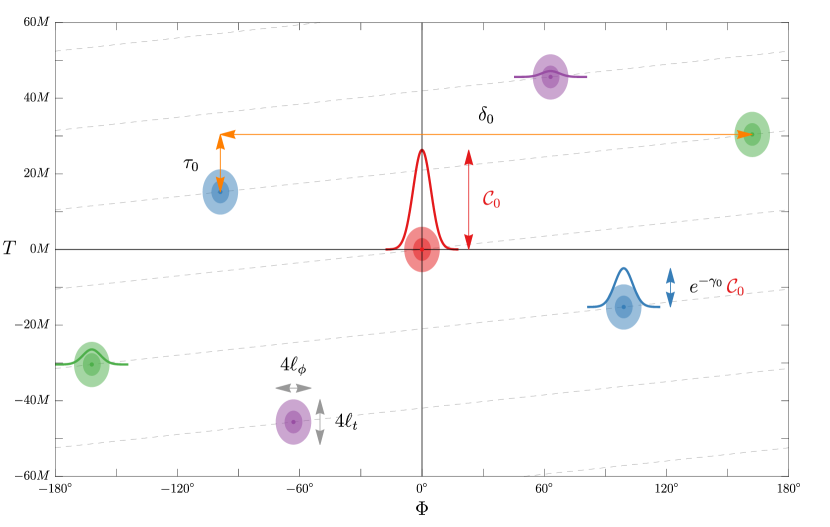
Figure 13: The characteristic structure of the photon ring autocorrelation function $\mathcal{C}(T,\varphi_{0},\varphi_{0}+\Phi$) for a fiducial value $\varphi_{0}$. The relations between correlation peaks are determined by the critical exponents $\gamma$, $\delta$, and $\tau$ (shown here with a $0$ subscript denoting a polar observer) and therefore universal; on the other hand, the details $\mathcal{C}_{0}$, $l_{t}$, $l_{\phi}$ of the fluctuations are not universal as they are emission-dependent. This is Figure 1 from Hadar2021 ; see the caption therein for additional details.

At least in principle, since the autocorrelation function is determined by the critical exponents, measuring these correlations effectively measures these exponents. Since these exponents are extremely sensitive to changes of the underlying metric (see, e.g. ,JohnsonLupsasca2020 ; Staelens2023 ), the autocorrelation function represents an exciting avenue for performing a precision test of the underlying black hole geometry. It was estimated in Hadar2021 that, for M87^∗ observations, detecting a strong signal in $\mathcal{C}$ may require many months or years of observations; with some optimism, a first estimate of $\mathcal{C}$ could be possible with EHT observations of M87^∗ every few days over a span of a few months or years Hadar2021 . The situation may be (orders of magnitude) more optimistic for first estimates of $\mathcal{C}$ (i.e., the red and blue peaks in Figure 13) for Sgr A^∗, although even there years of continuous observation would be necessary to resolve the second and higher-order correlation peaks (the purple and green peaks in Figure 13) Hadar2021 .

0.4 Testing general relativity in practice

The previous Section focused on identifying possible observables in black hole images that could, in principle, give unambiguous information on the underlying black hole geometry. Now, we turn to the question of how these observables could be leveraged into actual tests of GR.

To set the scene, we will first give a lightning overview of how and why GR can be expected to be corrected, and how possible deviations are modelled in practice. Then, we will highlight the important difference between consistency and discriminatory tests of GR. Finally, we give a few examples of both types of tests, and discuss the present and (near-)future prospects for such tests via VLBI observations.

0.4.1 What could lie beyond general relativity?

The idea of testing GR naturally raises the question: what else could there be? How could (or will) GR be corrected or changed? Here, we review the main possibilities that are typically considered in beyond-GR phenomenology and especially in black hole imaging.

Black holes truly open a new window into the “strong-field” regime of gravity. First of all, the Newtonian potential $GM/(Rc^{2})$ becomes of order unity near the horizon. Additionally, at least for relatively small (stellar-mass) black holes, the curvature scales involved near the horizon are much larger than any other curvatures that affect any measurements of gravitational observables. See, e.g., Psaltis2019 for further discussion.

GR predicts its own downfall by requiring the existence of intrinsic curvature singularities inside of black holes, past which geodesics become nonextendable. A slightly more subtle issue with black holes in GR is the information paradox Mathur2009 , which arises from considering fluctuating quantum fields around a black hole horizon (instead of at the singularity).

A natural assumption would be that a full, ultraviolet-complete theory of quantum gravity should somehow regularize the infinities at the black hole curvature singularities and resolve the information paradox satisfactorily. Of course, it is notoriously difficult to quantize gravity, and the resolution of the various apparent paradoxes posed by black holes is certainly not a settled theoretical problem within GR—in particular, it is unclear what (observable) changes to make to classical GR.

Therefore, it is natural to instead characterize possible corrections to GR in an agnostic way. An EFT approach—the gold standard in particle physics—would proceed by enumerating possible corrections to GR; in pure gravity, these are higher-derivative corrections in the action Endlich2017 :

$$S_{EFT} =\frac{1}{16\pi G}\int\mathop{}\!\mathrm{d}^{4}x\sqrt{-g}\left(R\right.$$

$$\left.+\lambda_{\rm ev}R\indices{{}_{\mu\nu}^{\rho\sigma}}R\indices{{}_{\rho\sigma}^{\delta\gamma}}R\indices{{}_{\delta\gamma}^{\mu\nu}}+\lambda_{\rm odd}R\indices{{}_{\mu\nu}^{\rho\sigma}}R\indices{{}_{\rho\sigma}^{\delta\gamma}}\epsilon_{\delta\gamma\alpha\beta}R\indices{{}^{\alpha\beta}{}^{\mu\nu}}\right)$$

where we have included the most general correction to GR involving at most six derivatives acting on the metric Endlich2017 ; Cano2019 . Four-derivative curvature corrections are total derivatives in four dimensions; however, if other matter fields such as a scalar are included as well, the four-derivative corrections can couple to these fields and become dynamical as well. The most prominent examples of such four-derivative gravity theories coupled to scalars are Einstein-dilaton-Gauss-Bonnet (EdGB) theory and dynamical Chern-Simons (dCS) theory Cano2019 ; Alexander2009 . By simulating what the observable effects of these higher-derivative couplings would be, bounds can then be put on the size of the couplings with current (and future) detections. See, e.g., Okounkova2019 for a derivation of the critical curve in dCS theory, and Deich2023 for a recent study of the dCS deviations in the Lyapunov exponent.

The coupling constants $\lambda_{\text{odd,ev}}$ in (0.4.1) have dimension $[\text{length}]^{4}$ and so are naturally suppressed by powers of the Planck scale ($\sim 10^{-35}\,m$). Higher corrections would come with even higher powers of the curvature and so would be even further suppressed. The curvatures involved in observable properties of black holes are very far from the Planck scale: for a solar-mass black hole, the curvature scale at the (Schwarzschild) horizon is of the order of a kilometer; a supermassive black hole (such as M87^∗ or Sgr A^∗) has curvatures at the horizon that are six or more orders of magnitude smaller. The natural size of the coupling constants is then many orders of magnitude smaller than any reasonable bound that could ever be placed on them from any observations. From an EFT perspective, therefore, the natural expectation is that observations will effectively never reveal deviations from GR due to these higher-derivative corrections.

However, this “standard” EFT reasoning may fail in a number of ways. Of course, the “natural” scale for the higher-derivative corrections may not be the correct scale. (Recall, for example, that the “natural” scale for the cosmological constant is about $10^{120}$ orders of magnitude larger than the actual observed value!) We will mention three other important caveats to this EFT “naturalness” argument. First of all, quantum effects may become important even at curvature scales well below where EFT predicts they should become appreciable. In string theory, the fuzzball paradigm Mathur2005 ; Mayerson2020 ; Mayerson2023 precisely hinges on arguments that the classical description of gravity breaks down at horizon scales—despite the absence of large curvatures. Instead, at the horizon scale, quantum, stringy effects take over to render the black hole radically different than its classical GR description; instead of a featureless horizon, spacetime is replaced at these scales by stringy “fuzz”; hence the “fuzzball” name.

A second caveat is that there may exist other dark matter fields that have so far been unobserved but nevertheless couple to gravity. Effects of such dark matter would be especially relevant for the physics of (e.g.) black hole mergers Barausse2020 , where various interactions between the black holes and the dark matter can give rise to interesting signatures in the observed gravitational-wave signal. In imaging phenomenology, the effects of (e.g.) dark matter halos around the observed supermassive black hole have been considered Hou2018 , as have the effects of ultralight bosons on the autocorrelation pattern of the photon ring Chen2023 .

A third caveat is that there may exist other, hitherto-unknown ultracompact exotic compact objects (ECOs). Such ECOs could be more compact than a neutron star but still less compact than a black hole, and have evaded detection up until now due to their compactness and lack of emission. This is also related to the first and second point above: a fuzzball is an example of a possible ECO, and ECOs often rely on the existence of additional (dark) matter fields to support their compact structure. For an overview of possible ECOs and their phenomenology, see Cardoso2019 .

In practice, there are a number of ways to analyze and parametrize possible strong-gravity phenomena beyond GR. A well-traveled path in black hole imaging is to parametrize deviations from the Kerr metric itself, without worrying about how such metric deviations represent a solution to any underlying theory. By construction, such parametrizations are then model-agnostic. An example of this is the Johannsen metric Johannsen2013 ; Johannsen2011 , which parametrizes the most general deviation from Kerr that still allows for separable geodesic equations.

Alternatively, one can consider solutions to alternative or corrected theories of gravity. For example, one can consider all possible pure gravitational corrections to GR arising from (0.4.1). It is also possible to take a theory of GR coupled to (dark) matter and consider solutions of such theories that are similar but different to Kerr. Perhaps the simplest example is the Kerr-Newman black hole, which is a solution to Einstein-Maxwell theory. Another example is the theory obtained by minimally coupling a scalar field to GR, which leads to the existence of “hairy” black holes Herdeiro2014 ; Herdeiro2015 as well as horizonless ECOs called boson stars. The fuzzballs mentioned above are also a type of ultracompact ECO Mathur2005 ; Mayerson2020 ; these are complex solutions to certain supergravity theories (i.e., theories of gravity coupled to various scalar and gauge fields) and are posited in string theory to be the individual microstates of a black hole—meaning that counting these microstates should reproduce the black hole’s entropy. Images of boson stars and hairy black holes have been studied in, e.g., Cunha2015 ; Cunha2016 ; Vincent2016 ; Olivares2020 ; rudimentary fuzzball imaging has been analyzed in Bacchini2021 .

The above approaches all involve classical gravity theories or geometries, and are essentially devoid of true quantum corrections to gravity. Investigating (measurable) quantum effects in imaging is also more or less unexplored territory, with perhaps a few notable exceptions such as Giddings2018 , although even there the quantum effects are posited to lead to observable coherent (classical) fluctuations of the metric.

0.4.2 Consistency tests versus discriminatory tests

Testing GR in observations goes hand-in-hand with looking for beyond-GR effects, either in the form of corrections to black hole metrics or new ECOs as discussed in the previous Section. One can make a distinction between two different types of tests of GR:

• Consistency tests, or null tests, in which GR is shown to be consistent (or not) with the observed data up to a certain precision level; and

• Discriminatory tests, in which GR is tested against another, different theory, and it is shown that the observed data prefers either GR or the alternative theory.

In statistical terms, consistency tests correspond to a hypothesis test where the null hypothesis is GR and the alternative hypothesis is not-GR, whereas a discriminatory test could be a Bayesian model selection between GR and the alternative theory.

For example, GR predicts that the shape of the photon ring is a circlipse (see Section 0.3.4). Testing if and how well a measured photon ring shape fits the circlipse functional shape is then a consistency test of GR. However, the circlipse shape of the photon ring is fairly universal across many models of corrections to black hole physics (see Staelens2023 for examples and universality for an explanation why this is the case): in other words, Kerr and many other black holes beyond GR will all have photon rings that have circlipse shapes. This implies that fitting an observed photon ring shape to the circlipse functional form is not necessarily a good discriminatory test, since it has little distinguishing power between different theories.

Existing EHT observations are consistent with the theoretical modelling and expectations based on GRMHD-simulated accretion flows (see Section 0.2.4) onto a Kerr black hole EHT2019I ; EHT2019VI . In this sense, the EHT measurements are certainly a consistency test of GR. There has been vigorous debate as to the level of precision of this test Gralla2021 and how this level should even be defined. We take the view that the test is both obviously valuable, and also obviously rather imprecise (see, e.g.. Sections 0.2.3, 0.2.4 and 0.3.1). We are nearing a new era of precision black hole imaging (see below Section 0.4.4) in which much greater precision will be achieved in observations and thus in the level of precision in the (consistency) testing of GR.

It is important to stress that the level of precision that is achievable with a given test (whether a consistency or discriminatory test) depends on both the measurement precision, as well as the inherent uncertainties associated with the test. For example, we discussed the (image) shadow above (Section 0.3.1). The existence of such a shadow may be relatively robust over different plasma emission models Bronzwaer2021 , but the precise details—such as its size, for instance—do depend (however slightly) on the emission details. As long as that is true, there will be an inherent uncertainty associated with any test based on the details of the image shadow. Moreover, this uncertainty does not improve when better observations are made, except as a secondary effect of being able to better constrain the possible emission models.

0.4.3 What is (not) a test, with examples

In this Section, we give some examples of proposed tests, both of consistency and discriminatory. We also emphasize the most common pitfalls associated with such proposals. Our aim is not to be comprehensive in giving an overview of all proposed imaging-based tests of GR, but rather to sketch of the current status of the field.

Given a black hole that admits separable null geodesics, an simple analysis to carry out is to study how its critical curve deviates from Kerr; see, e.g.,Johannsen2010 ; Bambi2010 ; Abdujabbarov2013 ; Amarilla2013 ; Vincent2016 ; Giddings2018 ; Mureika2017 ; Chen2020 ; Uniyal2023b ; Uniyal2023b for a non-exhaustive list of examples. However, as in the above discussion in Section 0.3.1, we want to stress that this is only a first indication of how such deformations of Kerr might be observable, since the critical curve is not directly observable. For example, the critical curve will typically be close to, but not precisely at, the boundary of the image shadow for Kerr—but this is not obviously still the case in a deviating black hole metric. To provide further evidence of observable consequences of a change in critical curve, a next step could be an analysis generalizing the Kerr study of Bronzwaer2021 , i.e., analyzing the image shadow across different emission models on the alternative black hole metric in question.

The photon ring should also closely approximate the critical curve (although this should, once again, be verified for the alternative black hole). However, as discussed in Section 0.3.4, only the projected diameter is really relevant for the measurement of the photon ring (and thus critical curve) shape, so even seemingly quite different critical curves may give rise to the same interferometrically observed shape. In other words, to (only) look at the critical curve of a beyond-Kerr metric is certainly a good starting point to understand deviations of beyond-Kerr metrics in black hole imaging, but this analysis does not yet result in a good understanding of what interesting signals could arise from such a beyond-Kerr metric in interferometric observations.

The above example also illustrates a subtle pitfall in black hole imaging observations: a good test of GR should not revolve around a property of the image itself—rather, it should follow from a property of the visibility (i.e., the Fourier transform of the image), or even the visibility amplitude, since that is what is actually observed (see Section 0.2.3). Our intuition is not always well-suited to understanding how image features translate to features in the Fourier-transformed visibility (or vice versa), and features that seem distinctive in an image may not be so easily distinguished in the visibility.

With these subtle pitfalls in mind, we can discuss a few examples of proposed consistency and discriminatory tests. As aforementioned, the EHT observations provide a prime example of consistency tests. In particular, the observed mass and spin parameters of both M87^∗ and Sgr A^∗ are well within the expected range from other observations EHT2019I ; EHT2022I . Measuring the inner shadow (see Section 0.3.1) is a proposed consistency test that would be possible with the ngEHT Chael2021 .

Various consistency tests involving the photon rings have been proposed and studied in detail, including an estimate on (near-)future obtainable precision of these tests. Examples include GLM2020 for the shape of the $n=2$ ring (see Section 0.3.4), Paugnat2022 for further analysis of the $n=2$ ring shape over a range of simulated emission models, CardenasAvendano2023 for the observed shape of the $n=1$ ring. The photon ring autocorrelations (see Section 0.3.5) were discussed as a consistency test in Hadar2021 .

Currently developed discriminatory tests are fewer in number. There was a strong claim that measurements of the (image) shadow can be used to constrain post-Newtonian (PN) deviations to the metric Psaltis2020 , although it is not obvious how well-suited such a PN-expansion is for describing geodesics near bound orbits, as the PN expansion precisely breaks down near the horizon Volkel2021 ; see also Gralla2019 ; Gralla2021 . Other analyses show that constraints on beyond-Kerr parameters in the metric would only be rather weak Ayzenberg2022 , and that specifically the only type of models that could realistically be constrained are those with dimensionless parameters (and so certainly not corrections such as in (0.4.1)) Glampedakis2021 .

GRMHD simulations are quite computationally expensive. It is therefore perhaps remarkable that GRMHD plasma simulations have already been performed in a few models of beyond-GR compact objects, with the aim of investigating possible deviations in imaging observations. The difference in images of a Kerr versus a dilatonic black hole was analyzed in Mizuno2018 ; Fromm2021 ; Roder2023 ; a conclusion from these works is that it is again very difficult with current observation capabilities to distinguish Kerr black holes from other objects. In Olivares2020 , accretion flows onto horizonless boson stars were considered, leading to certain possible discriminatory signatures in imaging observations. Spherical accretion in certain alternative gravity theories was analyzed in Bauer2022 . Relatedly, GRMHD simulations in a large class of non-vacuum spacetimes was considered in Kocherlakota2023 . Finally, the EHT collaboration has tested some basic image properties of a number of analytic metrics in the context of the first Sgr A^∗ observations EHT2022VI .

It is perhaps somewhat surprising how few attempts have been made at discriminatory tests involving the photon rings, given our focus on observables involving them in Section 0.3. The theoretical derivation of the photon rings in Kerr is crucially linked to the critical curve corresponding to bound photon orbits (see Section 0.2.2). For geometries beyond Kerr, the separability of the geodesic equations (generically) should not hold, rendering the entire reasoning that led to the derivation of the critical curve moot—does a single, connected critical curve exist for generic beyond-Kerr black holes (or other ultracompact objects)? Probably not Staelens2023 . What are the effects on the various properties of the photon rings? And even for metrics allowing for separable geodesic equations, how are the properties of the photon ring altered, such as its shape and critical exponents? A first attempt to answer such questions was made in Staelens2023 in the context of the Lyapunov exponent and photon ring shape for simple black hole metrics admitting separable geodesic equations. As mentioned above, it was found that the photon ring circlipse shape, while a good consistency test of GR, is too generic to be able to distinguish between different models; the underlying reason for this universality was further exposed in universality . Another recent advance was the development of a formalism to define and calculate the Lyapunov critical exponent for generic metrics without geodesic separability Deich2023 . Finally, very recently a discriminatory test was proposed based on the lensing band structure of a beyond-Kerr spacetime: in essence, the idea is that if a photon ring is observed, its position can be used to rule out models where the observed photon ring does not fit in the model’s lensing band CardenasAvendano2024 . Evidently, there are still many photon ring properties that have not been considered yet in any discriminatory tests, leaving numerous interesting features of beyond-GR photon ring physics as yet to be explored.

0.4.4 Where we are now and what the future holds

Current EHT observations show a bright ring of diameter around $\sim 40-50\,\mu$as (for both M87^∗ and Sgr A^∗) surrounding a dark brightness depression. As we have discussed, this is already a type of consistency test of GR (see Sections 0.4.2 and 0.4.3).

The ngEHT will upgrade and expand the existing EHT telescope array with additional telescopes, improved observation methods, and greatly expanded observation durations Johnson2023 . Key science goals for the ngEHT include measuring properties of the photon ring as well as measuring the inner shadow (as a signature of the existence of the event horizon; see Sections 0.3.1) Ayzenberg2023 .

The current observations resolve the $n=0$ image, using photon ring terminology. However, the actual photon ring comprised of light that orbited around the black hole (i.e., the $n\geq 1$ images) has not yet been resolved, and requires longer baselines than can be accessed with a solely Earth-based telescope array. Future space-based VLBI missions Gurvits2022 ; Kurczynski2022 aim to extend the EHT to space via an orbiting satellite, so as to sample longer baselines and enable a measurement of the photon ring and some of the associated observables discussed in Sections 0.3.2, 0.3.3, 0.3.4, and 0.3.5. Such missions will open the door to more precise tests of GR in the strong-field regime. As we have discussed, the strong tests that are and will be possible are mostly consistency tests of GR and the Kerr metric, although there is also some potential for discriminatory tests using beyond-GR models.

The EHT has given us a first unprecedentedly close view of the horizon-scale emission from the close environment of two supermassive black holes. It is clear that observing light originating from and affected by the strong-field gravitational pull of a black hole is a compelling and necessary experiment to carry out and improve. Besides providing a way to qualitatively confirm predictions of strong-field GR, such experiments may also uncover crucial information about black hole spin, jet-launching, electromagnetic energy extraction, and other astrophysical phenomena of great interest. The future of black hole imaging is bright.

Appendix: Projected diameter

Here, following GrallaLupsasca2020c , we give the appropriate definition of projected diameter that is used in Section 0.3.4.

Given a closed curve in a plane, parametrized as $(x(\sigma),y(\sigma))$, one can define the normal angle to the curve by:

$$\tan{\varphi(\sigma)}=-\frac{x^{\prime}(\sigma)}{y^{\prime}(\sigma)}.$$ (0.4.1)

For convex curves, this can be inverted to obtain $\sigma(\varphi)$ and obtain a normal-angle parametrization $(x(\varphi),y(\varphi))$ (see GrallaLupsasca2020c for a prescription for non-convex curves). The projected position of the curve is then defined as:

$$f(\varphi)=x(\varphi)\cos{\varphi}+y(\varphi)\sin{\varphi},\qquad\varphi\in[0,2\pi).$$ (0.4.2)

Interestingly, this function fully encodes the curve, which may be reconstructed via

$$x(\varphi)=f(\varphi)\cos{\varphi}-f^{\prime}(\varphi)\sin{\varphi},\qquad y(\varphi)=f(\varphi)\sin{\varphi}+f^{\prime}(\varphi)\cos{\varphi}.$$ (0.4.3)

We can further decompose the projected position into its parity-even and parity-odd components:

$$d_{\varphi}=\frac{f(\varphi)+f(\varphi+\pi)}{2},\qquad C_{\varphi}=f(\varphi)-f(\varphi+\pi),\qquad\varphi\in[0,\pi),$$ (0.4.4)

where $d_{\varphi}$ is called the projected diameter and $C_{\varphi}$ is the projected centroid of the curve (see, e.g., Figure 3 in GrallaLupsasca2020c for further illustration).

In an elegant exercise in Fourier analysis, Gralla Gralla2020 showed that a bright and narrow curve with projected diameter and centroid $(d_{\varphi},C_{\varphi})$ produces an interferometric response along the polar angle $\varphi$ on the observer screen given by:

$$V(u,\varphi)\approx\frac{e^{-2\pi iC_{\varphi}}}{\sqrt{u}}\left(\alpha_{\varphi}^{\rm L}e^{-\frac{i\pi}{4}}e^{i\pi d_{\varphi}u}+\alpha_{\varphi}^{\rm R}e^{\frac{i\pi}{4}}e^{-i\pi d_{\varphi}u}\right),$$ (0.4.5)

The resulting visibility amplitude $|V(u,\varphi)|$, which is more robust to noise than the phase, is then given by (0.3.10), which only depends on the projected diameter $d_{\varphi}$.

References

- (1) Event Horizon Telescope Collaboration, “First M87 Event Horizon Telescope Results. I. The Shadow of the Supermassive Black Hole,” ApJ 875 no. 1, (Apr., 2019) L1, arXiv:1906.11238 [astro-ph.GA].
- (2) Event Horizon Telescope Collaboration, “First Sagittarius A* Event Horizon Telescope Results. I. The Shadow of the Supermassive Black Hole in the Center of the Milky Way,” arXiv e-prints (Nov., 2023) arXiv:2311.08680, arXiv:2311.08680 [astro-ph.HE].
- (3) M. D. Johnson, K. Akiyama, L. Blackburn, et al., “Key Science Goals for the Next-Generation Event Horizon Telescope,” Galaxies 11 no. 3, (Apr., 2023) 61, arXiv:2304.11188 [astro-ph.HE].
- (4) D. Ayzenberg, L. Blackburn, R. Brito, et al., “Fundamental Physics Opportunities with the Next-Generation Event Horizon Telescope,” arXiv e-prints (Dec., 2023) arXiv:2312.02130, arXiv:2312.02130 [astro-ph.HE].
- (5) L. I. Gurvits, Z. Paragi, R. I. Amils, et al., “The science case and challenges of space-borne sub-millimeter interferometry,” Acta Astronautica 196 (July, 2022) 314–333, arXiv:2204.09144 [astro-ph.IM].
- (6) A. Strominger and S. Carroll, “Sean Carroll’s Mindscape Podcast,” Jan., 2023. https://www.preposterousuniverse.com/podcast/2023/01/09/222-andrew-strominger-on-quantum-gravity-and-the-real-world/.
- (7) D. Psaltis, “Testing general relativity with the Event Horizon Telescope,” General Relativity and Gravitation 51 no. 10, (Oct., 2019) 137, arXiv:1806.09740 [astro-ph.HE].
- (8) J. M. Bardeen, “Timelike and null geodesics in the Kerr metric.,” in Black Holes (Les Astres Occlus), C. Dewitt and B. S. Dewitt, eds., pp. 215–239. Jan., 1973.
- (9) S. E. Gralla, A. Lupsasca, and A. Strominger, “Observational signature of high spin at the Event Horizon Telescope,” MNRAS 475 no. 3, (Apr., 2018) 3829–3853, arXiv:1710.11112 [astro-ph.HE].
- (10) B. Carter, “Global Structure of the Kerr Family of Gravitational Fields,” Physical Review 174 no. 5, (Oct., 1968) 1559–1571.
- (11) M. Walker and R. Penrose, “On quadratic first integrals of the geodesic equations for type { 22} spacetimes,” Communications in Mathematical Physics 18 no. 4, (Dec., 1970) 265–274.
- (12) D. Rasheed, “The rotating dyonic black holes of Kaluza-Klein theory,” Nuclear Physics B 454 (Feb., 1995) 379–401, arXiv:hep-th/9505038 [gr-qc].
- (13) F. Larsen, “Rotating Kaluza-Klein black holes,” Nuclear Physics B 575 no. 1-2, (May, 2000) 211–230, arXiv:hep-th/9909102 [hep-th].
- (14) C. Keeler and F. Larsen, “Separability of black holes in string theory,” Journal of High Energy Physics 2012 (Oct., 2012) 152, arXiv:1207.5928 [hep-th].
- (15) I. Bah, I. Bena, P. Heidmann, Y. Li, and D. R. Mayerson, “Gravitational footprints of black holes and their microstate geometries,” Journal of High Energy Physics 2021 no. 10, (Oct., 2021) 138, arXiv:2104.10686 [hep-th].
- (16) S. Staelens, “Black Hole Photon Rings Beyond General Relativity,” 2022. https://www.scriptiebank.be/sites/default/files/thesis/2022-09/Master_Thesis_Seppe_Staelens.pdf. Master’s thesis.
- (17) S. E. Gralla and A. Lupsasca, “Null geodesics of the Kerr exterior,” Phys. Rev. D 101 no. 4, (Feb., 2020) 044032, arXiv:1910.12881 [gr-qc].
- (18) S. Chandrasekhar, The mathematical theory of black holes. Oxford University Press, 1992.
- (19) P. A. Connors and R. F. Stark, “Observable gravitational effects on polarised radiation coming from near a black hole,” Nature 269 no. 5624, (Sept., 1977) 128–129.
- (20) P. A. Connors, T. Piran, and R. F. Stark, “Polarization features of X-ray radiation emitted near black holes.,” ApJ 235 (Jan, 1980) 224–244.
- (21) L.-X. Li, R. Narayan, and J. E. McClintock, “Inferring the Inclination of a Black Hole Accretion Disk from Observations of its Polarized Continuum Radiation,” ApJ 691 no. 1, (Jan., 2009) 847–865, arXiv:0809.0866 [astro-ph].
- (22) J. Dexter, “A public code for general relativistic, polarised radiative transfer around spinning black holes,” MNRAS 462 no. 1, (Oct., 2016) 115–136, arXiv:1602.03184 [astro-ph.HE].
- (23) D. Gates, D. Kapec, A. Lupsasca, Y. Shi, and A. Strominger, “Polarization Whorls from M87* at the Event Horizon Telescope,” arXiv e-prints (Sept., 2018) arXiv:1809.09092, arXiv:1809.09092 [hep-th].
- (24) E. Himwich, M. D. Johnson, A. Lupsasca, and A. Strominger, “Universal polarimetric signatures of the black hole photon ring,” Phys. Rev. D 101 no. 8, (Apr., 2020) 084020, arXiv:2001.08750 [gr-qc].
- (25) R. Narayan, D. C. M. Palumbo, M. D. Johnson, et al., “The Polarized Image of a Synchrotron-emitting Ring of Gas Orbiting a Black Hole,” ApJ 912 no. 1, (May, 2021) 35, arXiv:2105.01804 [astro-ph.HE].
- (26) Z. Gelles, E. Himwich, M. D. Johnson, and D. C. M. Palumbo, “Polarized image of equatorial emission in the Kerr geometry,” Phys. Rev. D 104 no. 4, (Aug., 2021) 044060, arXiv:2105.09440 [gr-qc].
- (27) D. Kapec and A. Lupsasca, “Particle motion near high-spin black holes,” Classical and Quantum Gravity 37 no. 1, (Jan., 2020) 015006, arXiv:1905.11406 [hep-th].
- (28) D. Hilbert, “Die Grundlagen der Physik. (Zweite Mitteilung),” Nachrichten von der Gesellschaft der Wissenschaften zu Göttingen, Mathematisch-Physikalische Klasse 1917 (1917) 53–76. http://eudml.org/doc/58973.
- (29) C. Darwin, “The Gravity Field of a Particle,” Proceedings of the Royal Society of London Series A 249 no. 1257, (Jan, 1959) 180–194.
- (30) M. D. Johnson, A. Lupsasca, A. Strominger, et al., “Universal interferometric signatures of a black hole’s photon ring,” Science Advances 6 no. 12, (Mar., 2020) eaaz1310, arXiv:1907.04329 [astro-ph.IM].
- (31) K. P. Rauch and R. D. Blandford, “Optical Caustics in a Kerr Spacetime and the Origin of Rapid X-Ray Variability in Active Galactic Nuclei,” ApJ 421 (Jan, 1994) 46.
- (32) S. E. Vázquez and E. P. Esteban, “Strong-field gravitational lensing by a Kerr black hole,” Nuovo Cimento B Serie 119 no. 5, (May, 2004) 489, arXiv:gr-qc/0308023 [gr-qc].
- (33) L.-X. Li, E. R. Zimmerman, R. Narayan, and J. E. McClintock, “Multitemperature Blackbody Spectrum of a Thin Accretion Disk around a Kerr Black Hole: Model Computations and Comparison with Observations,” ApJS 157 no. 2, (Apr., 2005) 335–370, arXiv:astro-ph/0411583 [astro-ph].
- (34) S. Staelens, D. R. Mayerson, F. Bacchini, B. Ripperda, and L. Küchler, “Black hole photon rings beyond general relativity,” Phys. Rev. D 107 no. 12, (June, 2023) 124026, arXiv:2303.02111 [gr-qc].
- (35) K. Beckwith and C. Done, “Extreme gravitational lensing near rotating black holes,” MNRAS 359 no. 4, (Jun, 2005) 1217–1228, arXiv:astro-ph/0411339 [astro-ph].
- (36) S. E. Gralla, D. E. Holz, and R. M. Wald, “Black hole shadows, photon rings, and lensing rings,” Phys. Rev. D 100 no. 2, (July, 2019) 024018, arXiv:1906.00873 [astro-ph.HE].
- (37) J. P. Luminet, “Image of a spherical black hole with thin accretion disk.,” A&A 75 (May, 1979) 228–235.
- (38) H. Paugnat, A. Lupsasca, F. H. Vincent, and M. Wielgus, “Photon ring test of the Kerr hypothesis: Variation in the ring shape,” A&A 668 (Dec., 2022) A11, arXiv:2206.02781 [astro-ph.HE].
- (39) A. Cárdenas-Avendaño and A. Lupsasca, “Prediction for the interferometric shape of the first black hole photon ring,” Phys. Rev. D 108 no. 6, (Sept., 2023) 064043, arXiv:2305.12956 [gr-qc].
- (40) S. E. Gralla and A. Lupsasca, “Lensing by Kerr black holes,” Phys. Rev. D 101 no. 4, (Feb., 2020) 044031, arXiv:1910.12873 [gr-qc].
- (41) E. Teo, “Spherical Photon Orbits Around a Kerr Black Hole,” General Relativity and Gravitation 35 no. 11, (Nov., 2003) 1909–1926.
- (42) S. Hadar, M. D. Johnson, A. Lupsasca, and G. N. Wong, “Photon ring autocorrelations,” Phys. Rev. D 103 no. 10, (May, 2021) 104038, arXiv:2010.03683 [gr-qc].
- (43) M. Wielgus, “Photon rings of spherically symmetric black holes and robust tests of non-Kerr metrics,” Phys. Rev. D 104 no. 12, (Dec., 2021) 124058, arXiv:2109.10840 [gr-qc].
- (44) D. Ayzenberg, “Testing gravity with black hole shadow subrings,” Classical and Quantum Gravity 39 no. 10, (May, 2022) 105009, arXiv:2202.02355 [gr-qc].
- (45) E. Omwoyo, H. Belich, J. C. Fabris, and H. Velten, “Black hole lensing in Kerr-de Sitter spacetimes,” European Physical Journal Plus 138 no. 11, (Nov., 2023) 1043, arXiv:2212.10492 [gr-qc].
- (46) G. J. Olmo, J. L. Rosa, D. Rubiera-Garcia, and D. Sáez-Chillón Gómez, “Shadows and photon rings of regular black holes and geonic horizonless compact objects,” Classical and Quantum Gravity 40 no. 17, (Sept., 2023) 174002, arXiv:2302.12064 [gr-qc].
- (47) A. Deich, N. Yunes, and C. Gammie, “Lyapunov Exponents to Test General Relativity,” arXiv e-prints (Aug., 2023) arXiv:2308.07232, arXiv:2308.07232 [gr-qc].
- (48) D. H. Roberts, J. F. C. Wardle, and L. F. Brown, “Linear Polarization Radio Imaging at Milliarcsecond Resolution,” ApJ 427 (June, 1994) 718.
- (49) P. H. van Cittert, “Die Wahrscheinliche Schwingungsverteilung in Einer von Einer Lichtquelle Direkt Oder Mittels Einer Linse Beleuchteten Ebene,” Physica 1 no. 1, (Jan., 1934) 201–210.
- (50) F. Zernike, “The concept of degree of coherence and its application to optical problems,” Physica 5 no. 8, (Aug., 1938) 785–795.
- (51) Event Horizon Telescope Collaboration, “First M87 Event Horizon Telescope Results. IV. Imaging the Central Supermassive Black Hole,” ApJ 875 no. 1, (Apr., 2019) L4, arXiv:1906.11241 [astro-ph.GA].
- (52) Event Horizon Telescope Collaboration, “First M87 Event Horizon Telescope Results. V. Physical Origin of the Asymmetric Ring,” ApJ 875 no. 1, (Apr., 2019) L5, arXiv:1906.11242 [astro-ph.GA].
- (53) Event Horizon Telescope Collaboration, “First Sagittarius A* Event Horizon Telescope Results. V. Testing Astrophysical Models of the Galactic Center Black Hole,” ApJ 930 no. 2, (May, 2022) L16.
- (54) Event Horizon Telescope Collaboration, “First Sagittarius A* Event Horizon Telescope Results. IV. Variability, Morphology, and Black Hole Mass,” ApJ 930 no. 2, (May, 2022) L15.
- (55) Event Horizon Telescope Collaboration, “First M87 Event Horizon Telescope Results. VI. The Shadow and Mass of the Central Black Hole,” ApJ 875 no. 1, (Apr., 2019) L6, arXiv:1906.11243 [astro-ph.GA].
- (56) J. Davelaar, B. Ripperda, L. Sironi, et al., “Synchrotron Polarization Signatures of Surface Waves in Supermassive Black Hole Jets,” ApJ 959 no. 1, (Dec., 2023) L3, arXiv:2309.07963 [astro-ph.HE].
- (57) K. Parfrey, A. Philippov, and B. Cerutti, “First-Principles Plasma Simulations of Black-Hole Jet Launching,” Phys. Rev. Lett. 122 no. 3, (Jan., 2019) 035101, arXiv:1810.03613 [astro-ph.HE].
- (58) B. Crinquand, B. Cerutti, G. Dubus, K. Parfrey, and A. Philippov, “Synthetic Images of Magnetospheric Reconnection-Powered Radiation around Supermassive Black Holes,” Phys. Rev. Lett. 129 no. 20, (Nov., 2022) 205101, arXiv:2202.04472 [astro-ph.HE].
- (59) A. Galishnikova, A. Philippov, E. Quataert, et al., “Collisionless Accretion onto Black Holes: Dynamics and Flares,” Phys. Rev. Lett. 130 no. 11, (Mar., 2023) 115201, arXiv:2212.02583 [astro-ph.HE].
- (60) F. Bacchini, B. Ripperda, O. Porth, and L. Sironi, “Generalized, Energy-conserving Numerical Simulations of Particles in General Relativity. II. Test Particles in Electromagnetic Fields and GRMHD,” ApJS 240 no. 2, (Feb., 2019) 40, arXiv:1810.00842 [astro-ph.HE].
- (61) F. Bacchini, B. Ripperda, A. A. Philippov, and K. Parfrey, “A Coupled Guiding Center-Boris Particle Pusher for Magnetized Plasmas in Compact-object Magnetospheres,” ApJS 251 no. 1, (Nov., 2020) 10, arXiv:2007.14401 [astro-ph.HE].
- (62) A. Levinson and B. Cerutti, “Particle-in-cell simulations of pair discharges in a starved magnetosphere of a Kerr black hole,” A&A 616 (Aug., 2018) A184, arXiv:1803.04427 [astro-ph.HE].
- (63) B. Crinquand, B. Cerutti, A. Philippov, K. Parfrey, and G. Dubus, “Multidimensional Simulations of Ergospheric Pair Discharges around Black Holes,” Phys. Rev. Lett. 124 no. 14, (Apr., 2020) 145101, arXiv:2003.03548 [astro-ph.HE].
- (64) A. Y. Chen and Y. Yuan, “Physics of Pair Producing Gaps in Black Hole Magnetospheres. II. General Relativity,” ApJ 895 no. 2, (June, 2020) 121, arXiv:1908.06919 [astro-ph.HE].
- (65) M. D. Duez, Y. T. Liu, S. L. Shapiro, and B. C. Stephens, “Relativistic magnetohydrodynamics in dynamical spacetimes: Numerical methods and tests,” Phys. Rev. D 72 no. 2, (July, 2005) 024028, arXiv:astro-ph/0503420 [astro-ph].
- (66) M. Shibata and Y.-I. Sekiguchi, “Magnetohydrodynamics in full general relativity: Formulation and tests,” Phys. Rev. D 72 no. 4, (Aug., 2005) 044014, arXiv:astro-ph/0507383 [astro-ph].
- (67) M. Anderson, E. W. Hirschmann, L. Lehner, et al., “Magnetized Neutron-Star Mergers and Gravitational-Wave Signals,” Phys. Rev. Lett. 100 no. 19, (May, 2008) 191101, arXiv:0801.4387 [gr-qc].
- (68) P. Mösta, B. C. Mundim, J. A. Faber, et al., “GRHydro: a new open-source general-relativistic magnetohydrodynamics code for the Einstein toolkit,” Classical and Quantum Gravity 31 no. 1, (Jan., 2014) 015005, arXiv:1304.5544 [gr-qc].
- (69) E. R. Most, L. J. Papenfort, and L. Rezzolla, “Beyond second-order convergence in simulations of magnetized binary neutron stars with realistic microphysics,” MNRAS 490 no. 3, (Dec., 2019) 3588–3600, arXiv:1907.10328 [astro-ph.HE].
- (70) P. C.-K. Cheong, L.-M. Lin, and T. G. F. Li, “Gmunu: toward multigrid based Einstein field equations solver for general-relativistic hydrodynamics simulations,” Classical and Quantum Gravity 37 no. 14, (July, 2020) 145015, arXiv:2001.05723 [gr-qc].
- (71) L. Combi and D. M. Siegel, “GRMHD Simulations of Neutron-star Mergers with Weak Interactions: r-process Nucleosynthesis and Electromagnetic Signatures of Dynamical Ejecta,” ApJ 944 no. 1, (Feb., 2023) 28, arXiv:2206.03618 [astro-ph.HE].
- (72) W. Cook, B. Daszuta, J. Fields, et al., “GR-Athena++: General-relativistic magnetohydrodynamics simulations of neutron star spacetimes,” arXiv e-prints (Nov., 2023) arXiv:2311.04989, arXiv:2311.04989 [gr-qc].
- (73) O. Porth, K. Chatterjee, R. Narayan, et al., “The Event Horizon General Relativistic Magnetohydrodynamic Code Comparison Project,” ApJS 243 no. 2, (Aug., 2019) 26, arXiv:1904.04923 [astro-ph.HE].
- (74) B. Ripperda, M. Liska, K. Chatterjee, et al., “Black Hole Flares: Ejection of Accreted Magnetic Flux through 3D Plasmoid-mediated Reconnection,” ApJ 924 no. 2, (Jan., 2022) L32, arXiv:2109.15115 [astro-ph.HE].
- (75) H. Hakobyan, B. Ripperda, and A. A. Philippov, “Radiative Reconnection-powered TeV Flares from the Black Hole Magnetosphere in M87,” ApJ 943 no. 2, (Feb., 2023) L29, arXiv:2209.02105 [astro-ph.HE].
- (76) V. Zhdankin, B. Ripperda, and A. A. Philippov, “Particle acceleration by magnetic Rayleigh-Taylor instability: Mechanism for flares in black hole accretion flows,” Physical Review Research 5 no. 4, (Oct., 2023) 043023, arXiv:2302.05276 [astro-ph.HE].
- (77) S. M. Ressler, C. J. White, E. Quataert, and J. M. Stone, “Ab Initio Horizon-scale Simulations of Magnetically Arrested Accretion in Sagittarius A* Fed by Stellar Winds,” ApJ 896 no. 1, (June, 2020) L6, arXiv:2006.00005 [astro-ph.HE].
- (78) M. Bugli, L. Del Zanna, and N. Bucciantini, “Dynamo action in thick discs around Kerr black holes: high-order resistive GRMHD simulations.,” MNRAS 440 (May, 2014) L41–L45.
- (79) S. M. Ressler, A. Tchekhovskoy, E. Quataert, M. Chandra, and C. F. Gammie, “Electron thermodynamics in GRMHD simulations of low-luminosity black hole accretion,” MNRAS 454 no. 2, (Dec., 2015) 1848–1870, arXiv:1509.04717 [astro-ph.HE].
- (80) M. Chandra, C. F. Gammie, F. Foucart, and E. Quataert, “An Extended Magnetohydrodynamics Model for Relativistic Weakly Collisional Plasmas,” ApJ 810 no. 2, (Sept., 2015) 162, arXiv:1508.00878 [astro-ph.HE].
- (81) F. Foucart, M. Chandra, C. F. Gammie, and E. Quataert, “Evolution of accretion discs around a kerr black hole using extended magnetohydrodynamics,” MNRAS 456 no. 2, (Feb., 2016) 1332–1345, arXiv:1511.04445 [astro-ph.HE].
- (82) A. A. Chael, R. Narayan, and A. Sadowski, “Evolving non-thermal electrons in simulations of black hole accretion,” MNRAS 470 no. 2, (Sept., 2017) 2367–2386, arXiv:1704.05092 [astro-ph.HE].
- (83) M. Chandra, F. Foucart, and C. F. Gammie, “grim: A Flexible, Conservative Scheme for Relativistic Fluid Theories,” ApJ 837 no. 1, (Mar., 2017) 92, arXiv:1702.01106 [astro-ph.IM].
- (84) F. Foucart, M. Chandra, C. F. Gammie, E. Quataert, and A. Tchekhovskoy, “How important is non-ideal physics in simulations of sub-Eddington accretion on to spinning black holes?,” MNRAS 470 no. 2, (Sept., 2017) 2240–2252, arXiv:1706.01533 [astro-ph.HE].
- (85) Q. Qian, C. Fendt, and C. Vourellis, “Jet Launching in Resistive GR-MHD Black Hole-Accretion Disk Systems,” ApJ 859 no. 1, (May, 2018) 28, arXiv:1804.09652 [astro-ph.HE].
- (86) B. Ripperda, F. Bacchini, O. Porth, et al., “General-relativistic Resistive Magnetohydrodynamics with Robust Primitive-variable Recovery for Accretion Disk Simulations,” ApJS 244 no. 1, (Sept., 2019) 10, arXiv:1907.07197 [physics.comp-ph].
- (87) C. Vourellis, C. Fendt, Q. Qian, and S. C. Noble, “GR-MHD Disk Winds and Jets from Black Holes and Resistive Accretion Disks,” ApJ 882 no. 1, (Sept., 2019) 2, arXiv:1907.10622 [astro-ph.HE].
- (88) B. Ripperda, F. Bacchini, and A. A. Philippov, “Magnetic Reconnection and Hot Spot Formation in Black Hole Accretion Disks,” ApJ 900 no. 2, (Sept., 2020) 100, arXiv:2003.04330 [astro-ph.HE].
- (89) E. R. Most and J. Noronha, “Dissipative magnetohydrodynamics for nonresistive relativistic plasmas: An implicit second-order flux-conservative formulation with stiff relaxation,” Phys. Rev. D 104 no. 10, (Nov., 2021) 103028, arXiv:2109.02796 [astro-ph.HE].
- (90) A. Nathanail, V. Mpisketzis, O. Porth, C. M. Fromm, and L. Rezzolla, “Magnetic reconnection and plasmoid formation in three-dimensional accretion flows around black holes,” MNRAS 513 no. 3, (July, 2022) 4267–4277, arXiv:2111.03689 [astro-ph.HE].
- (91) E. R. Most, J. Noronha, and A. A. Philippov, “Modelling general-relativistic plasmas with collisionless moments and dissipative two-fluid magnetohydrodynamics,” MNRAS 514 no. 4, (Aug., 2022) 4989–5003, arXiv:2111.05752 [astro-ph.HE].
- (92) J. Vos, H. Olivares, B. Cerutti, and M. Moscibrodzka, “Plasmoid identification and statistics in two-dimensional Harris sheet and GRMHD simulations,” arXiv e-prints (Sept., 2023) arXiv:2309.03267, arXiv:2309.03267 [astro-ph.HE].
- (93) A. Bransgrove, B. Ripperda, and A. Philippov, “Magnetic Hair and Reconnection in Black Hole Magnetospheres,” Phys. Rev. Lett. 127 no. 5, (July, 2021) 055101, arXiv:2109.14620 [astro-ph.HE].
- (94) I. V. Igumenshchev, R. Narayan, and M. A. Abramowicz, “Three-dimensional Magnetohydrodynamic Simulations of Radiatively Inefficient Accretion Flows,” ApJ 592 no. 2, (Aug., 2003) 1042–1059, arXiv:astro-ph/0301402 [astro-ph].
- (95) R. Narayan, I. V. Igumenshchev, and M. A. Abramowicz, “Magnetically Arrested Disk: an Energetically Efficient Accretion Flow,” PASJ 55 (Dec., 2003) L69–L72, arXiv:astro-ph/0305029 [astro-ph].
- (96) G. S. Bisnovatyi-Kogan and A. A. Ruzmaikin, “The Accretion of Matter by a Collapsing Star in the Presence of a Magnetic Field,” Ap&SS 28 no. 1, (May, 1974) 45–59.
- (97) G. S. Bisnovatyi-Kogan and A. A. Ruzmaikin, “The Accretion of Matter by a Collapsing Star in the Presence of a Magnetic Field. II: Self-consistent Stationary Picture,” Ap&SS 42 no. 2, (July, 1976) 401–424.
- (98) K. Chatterjee and R. Narayan, “Flux Eruption Events Drive Angular Momentum Transport in Magnetically Arrested Accretion Flows,” ApJ 941 no. 1, (Dec., 2022) 30, arXiv:2210.08045 [astro-ph.HE].
- (99) H. Jia, B. Ripperda, E. Quataert, et al., “Millimeter observational signatures of flares in magnetically arrested black hole accretion models,” MNRAS 526 no. 2, (Dec., 2023) 2924–2941, arXiv:2301.09014 [astro-ph.HE].
- (100) M. Najafi-Ziyazi, J. Davelaar, Y. Mizuno, and O. Porth, “Flares in the Galactic Centre II: polarisation signatures of flares at mm-wavelengths,” arXiv e-prints (Aug., 2023) arXiv:2308.16740, arXiv:2308.16740 [astro-ph.HE].
- (101) Z. Gelles, K. Chatterjee, M. Johnson, B. Ripperda, and M. Liska, “Relativistic Signatures of Flux Eruption Events near Black Holes,” Galaxies 10 no. 6, (Nov., 2022) 107, arXiv:2210.07273 [astro-ph.HE].
- (102) M. Liska, A. Tchekhovskoy, and E. Quataert, “Large-scale poloidal magnetic field dynamo leads to powerful jets in GRMHD simulations of black hole accretion with toroidal field,” MNRAS 494 no. 3, (May, 2020) 3656–3662, arXiv:1809.04608 [astro-ph.HE].
- (103) J. Jacquemin-Ide, F. Rincon, A. Tchekhovskoy, and M. Liska, “Magnetorotational dynamo can generate large-scale vertical magnetic fields in 3D GRMHD simulations of accreting black holes,” arXiv e-prints (Oct., 2023) arXiv:2311.00034, arXiv:2311.00034 [astro-ph.HE].
- (104) H. Jia, C. J. White, E. Quataert, and S. M. Ressler, “Observational signatures of black hole accretion: rotating versus spherical flows with tilted magnetic fields,” MNRAS 515 no. 1, (Sept., 2022) 1392–1403, arXiv:2201.08431 [astro-ph.HE].
- (105) L. Murchikova, C. J. White, and S. M. Ressler, “Remarkable Correspondence of the Sagittarius A* Submillimeter Variability with a Stellar-wind-fed Accretion Flow Model,” ApJ 932 no. 2, (June, 2022) L21, arXiv:2204.06170 [astro-ph.HE].
- (106) M. Guo, J. M. Stone, C.-G. Kim, and E. Quataert, “Toward Horizon-scale Accretion onto Supermassive Black Holes in Elliptical Galaxies,” ApJ 946 no. 1, (Mar., 2023) 26, arXiv:2211.05131 [astro-ph.HE].
- (107) S. M. Ressler, C. J. White, and E. Quataert, “Wind-Fed GRMHD Simulations of Sagittarius A*: Tilt and Alignment of Jets and Accretion Discs, Electron Thermodynamics, and Multi-Scale Modeling of the Rotation Measure,” arXiv e-prints (Mar., 2023) arXiv:2303.15503, arXiv:2303.15503 [astro-ph.HE].
- (108) K. Chatterjee, Z. Younsi, M. Liska, et al., “Observational signatures of disc and jet misalignment in images of accreting black holes,” MNRAS 499 no. 1, (Nov., 2020) 362–378, arXiv:2002.08386 [astro-ph.GA].
- (109) C. J. White, J. Dexter, O. Blaes, and E. Quataert, “The Effects of Tilt on the Images of Black Hole Accretion Flows,” ApJ 894 no. 1, (May, 2020) 14, arXiv:2001.02361 [astro-ph.HE].
- (110) C. J. White and E. Quataert, “The Effects of Tilt on the Time Variability of Millimeter and Infrared Emission from Sagittarius A*,” ApJ 926 no. 2, (Feb., 2022) 136, arXiv:2104.12896 [astro-ph.HE].
- (111) K. Chatterjee, M. Liska, A. Tchekhovskoy, and S. Markoff, “Misaligned magnetized accretion flows onto spinning black holes: magneto-spin alignment, outflow power and intermittent jets,” arXiv e-prints (Nov., 2023) arXiv:2311.00432, arXiv:2311.00432 [astro-ph.HE].
- (112) R. Blandford and N. Globus, “Ergomagnetosphere, ejection disc, magnetopause in M87 - I. Global flow of mass, angular momentum, energy, and current,” MNRAS 514 no. 4, (Aug., 2022) 5141–5158, arXiv:2204.11995 [astro-ph.HE].
- (113) F. Bacchini, B. Ripperda, A. Y. Chen, and L. Sironi, “Generalized, Energy-conserving Numerical Simulations of Particles in General Relativity. I. Time-like and Null Geodesics,” ApJS 237 no. 1, (July, 2018) 6, arXiv:1801.02378 [astro-ph.HE].
- (114) R. Gold, A. E. Broderick, Z. Younsi, et al., “Verification of Radiative Transfer Schemes for the EHT,” ApJ 897 no. 2, (July, 2020) 148.
- (115) B. S. Prather, J. Dexter, M. Moscibrodzka, et al., “Comparison of Polarized Radiative Transfer Codes Used by the EHT Collaboration,” ApJ 950 no. 1, (June, 2023) 35, arXiv:2303.12004 [astro-ph.HE].
- (116) G. N. Wong and L. Arzamasskiy, “Balanced Turbulence and the Helicity Barrier in Black Hole Accretion,” arXiv e-prints (Dec., 2023) arXiv:2312.16172, arXiv:2312.16172 [astro-ph.HE].
- (117) A. Galishnikova, A. Philippov, and E. Quataert, “Polarized Anisotropic Synchrotron Emission and Absorption and Its Application to Black Hole Imaging,” ApJ 957 no. 2, (Nov., 2023) 103, arXiv:2309.10029 [astro-ph.HE].
- (118) S. E. Gralla, “Can the EHT M87 results be used to test general relativity?,” Phys. Rev. D 103 no. 2, (Jan., 2021) 024023, arXiv:2010.08557 [astro-ph.HE].
- (119) G. Lara, S. H. Völkel, and E. Barausse, “Separating astrophysics and geometry in black hole images,” Phys. Rev. D 104 no. 12, (Dec., 2021) 124041, arXiv:2110.00026 [gr-qc].
- (120) F. Özel, D. Psaltis, and Z. Younsi, “Black Hole Images as Tests of General Relativity: Effects of Plasma Physics,” ApJ 941 no. 1, (Dec., 2022) 88, arXiv:2111.01123 [astro-ph.HE].
- (121) A. M. Bauer, A. Cárdenas-Avendaño, C. F. Gammie, and N. Yunes, “Spherical Accretion in Alternative Theories of Gravity,” ApJ 925 no. 2, (Feb., 2022) 119, arXiv:2111.02178 [gr-qc].
- (122) S. E. Gralla, A. Lupsasca, and D. P. Marrone, “The shape of the black hole photon ring: A precise test of strong-field general relativity,” Phys. Rev. D 102 no. 12, (Dec., 2020) 124004, arXiv:2008.03879 [gr-qc].
- (123) A. Cárdenas-Avendaño, A. Lupsasca, and H. Zhu, “Adaptive analytical ray tracing of black hole photon rings,” Phys. Rev. D 107 no. 4, (Feb., 2023) 043030, arXiv:2211.07469 [gr-qc].
- (124) A. Chael, M. D. Johnson, and A. Lupsasca, “Observing the Inner Shadow of a Black Hole: A Direct View of the Event Horizon,” ApJ 918 no. 1, (Sept., 2021) 6, arXiv:2106.00683 [astro-ph.HE].
- (125) D. Lee and C. F. Gammie, “Disks as Inhomogeneous, Anisotropic Gaussian Random Fields,” ApJ 906 no. 1, (Jan., 2021) 39, arXiv:2011.07151 [astro-ph.IM].
- (126) O. Porth, H. Olivares, Y. Mizuno, et al., “The black hole accretion code,” Computational Astrophysics and Cosmology 4 no. 1, (May, 2017) 1, arXiv:1611.09720 [gr-qc].
- (127) H. Olivares, O. Porth, J. Davelaar, et al., “Constrained transport and adaptive mesh refinement in the Black Hole Accretion Code,” A&A 629 (Sept., 2019) A61, arXiv:1906.10795 [astro-ph.HE].
- (128) L. G. Fishbone and V. Moncrief, “Relativistic fluid disks in orbit around Kerr black holes.,” ApJ 207 (Aug., 1976) 962–976.
- (129) A. Cárdenas-Avendaño and A. Held, “A Lensing-Band Approach to Spacetime Constraints,” arXiv e-prints (Dec., 2023) arXiv:2312.06590, arXiv:2312.06590 [gr-qc].
- (130) D. R. Mayerson and F. Bacchini, “FOORT: Flexible Object-Oriented Ray Tracer.” In preparation. Current version available at https://github.com/drmayerson/FOORT.
- (131) S. E. Gralla, “Measuring the shape of a black hole photon ring,” Phys. Rev. D 102 no. 4, (Aug., 2020) 044017, arXiv:2005.03856 [astro-ph.HE].
- (132) S. E. Gralla and A. Lupsasca, “Observable shape of black hole photon rings,” Phys. Rev. D 102 no. 12, (Dec., 2020) 124003, arXiv:2007.10336 [gr-qc].
- (133) H. Falcke, F. Melia, and E. Agol, “Viewing the Shadow of the Black Hole at the Galactic Center,” ApJ 528 no. 1, (Jan., 2000) L13–L16, arXiv:astro-ph/9912263 [astro-ph].
- (134) R. Narayan, M. D. Johnson, and C. F. Gammie, “The Shadow of a Spherically Accreting Black Hole,” ApJ 885 no. 2, (Nov., 2019) L33, arXiv:1910.02957 [astro-ph.HE].
- (135) T. Bronzwaer and H. Falcke, “The Nature of Black Hole Shadows,” ApJ 920 no. 2, (Oct., 2021) 155, arXiv:2108.03966 [astro-ph.HE].
- (136) D. C. M. Palumbo and G. N. Wong, “Photon Ring Symmetries in Simulated Linear Polarization Images of Messier 87*,” ApJ 929 no. 1, (Apr., 2022) 49, arXiv:2203.00844 [astro-ph.HE].
- (137) D. C. M. Palumbo, G. N. Wong, A. Chael, and M. D. Johnson, “Demonstrating Photon Ring Existence with Single-baseline Polarimetry,” ApJ 952 no. 2, (Aug., 2023) L31, arXiv:2307.05293 [astro-ph.HE].
- (138) P. Kurczynski, M. D. Johnson, S. S. Doeleman, et al., “The Event Horizon Explorer mission concept,” in Space Telescopes and Instrumentation 2022: Optical, Infrared, and Millimeter Wave, L. E. Coyle, S. Matsuura, and M. D. Perrin, eds., vol. 12180 of Society of Photo-Optical Instrumentation Engineers (SPIE) Conference Series, p. 121800M. Aug., 2022.
- (139) G. N. Wong, “Black Hole Glimmer Signatures of Mass, Spin, and Inclination,” ApJ 909 no. 2, (Mar., 2021) 217, arXiv:2009.06641 [astro-ph.HE].
- (140) S. Hadar, S. Harikesh, and D. Chelouche, “Extreme lensing induces spectrotemporal correlations in black-hole signals,” Phys. Rev. D 107 no. 12, (June, 2023) 124057, arXiv:2305.11247 [gr-qc].
- (141) Y. Chen, X. Xue, R. Brito, and V. Cardoso, “Photon Ring Astrometry for Superradiant Clouds,” Phys. Rev. Lett. 130 no. 11, (Mar., 2023) 111401, arXiv:2211.03794 [gr-qc].
- (142) S. D. Mathur, “The information paradox: a pedagogical introduction,” Classical and Quantum Gravity 26 no. 22, (Nov., 2009) 224001, arXiv:0909.1038 [hep-th].
- (143) S. Endlich, V. Gorbenko, J. Huang, and L. Senatore, “An effective formalism for testing extensions to General Relativity with gravitational waves,” Journal of High Energy Physics 2017 no. 9, (Sept., 2017) 122, arXiv:1704.01590 [gr-qc].
- (144) P. A. Cano and A. Ruipérez, “Leading higher-derivative corrections to Kerr geometry,” Journal of High Energy Physics 2019 no. 5, (May, 2019) 189, arXiv:1901.01315 [gr-qc].
- (145) S. Alexander and N. Yunes, “Chern-Simons modified general relativity,” Phys. Rep. 480 no. 1-2, (Aug., 2009) 1–55, arXiv:0907.2562 [hep-th].
- (146) M. Okounkova, M. A. Scheel, and S. A. Teukolsky, “Numerical black hole initial data and shadows in dynamical Chern-Simons gravity,” Classical and Quantum Gravity 36 no. 5, (Mar., 2019) 054001, arXiv:1810.05306 [gr-qc].
- (147) E. Palti, “The Swampland: Introduction and Review,” Fortschritte der Physik 67 no. 6, (June, 2019) 1900037, arXiv:1903.06239 [hep-th].
- (148) S. D. Mathur, “The fuzzball proposal for black holes: an elementary review,” Fortschritte der Physik 53 no. 7-8, (July, 2005) 793–827, arXiv:hep-th/0502050 [hep-th].
- (149) D. R. Mayerson, “Fuzzballs and observations,” General Relativity and Gravitation 52 no. 12, (Dec., 2020) 115, arXiv:2010.09736 [hep-th].
- (150) D. R. Mayerson and B. Vercnocke, “Observational Opportunities for the Fuzzball Program,” arXiv e-prints (June, 2023) arXiv:2306.01565, arXiv:2306.01565 [hep-th].
- (151) E. Barausse, E. Berti, T. Hertog, et al., “Prospects for fundamental physics with LISA,” General Relativity and Gravitation 52 no. 8, (Aug., 2020) 81, arXiv:2001.09793 [gr-qc].
- (152) X. Hou, Z. Xu, M. Zhou, and J. Wang, “Black hole shadow of Sgr A∗ in dark matter halo,” J. Cosmology Astropart. Phys 2018 no. 7, (July, 2018) 015, arXiv:1804.08110 [gr-qc].
- (153) V. Cardoso and P. Pani, “Testing the nature of dark compact objects: a status report,” Living Reviews in Relativity 22 no. 1, (July, 2019) 4, arXiv:1904.05363 [gr-qc].
- (154) T. Johannsen, “Regular black hole metric with three constants of motion,” Phys. Rev. D 88 no. 4, (Aug., 2013) 044002, arXiv:1501.02809 [gr-qc].
- (155) T. Johannsen and D. Psaltis, “Metric for rapidly spinning black holes suitable for strong-field tests of the no-hair theorem,” Phys. Rev. D 83 no. 12, (June, 2011) 124015, arXiv:1105.3191 [gr-qc].
- (156) C. A. R. Herdeiro and E. Radu, “Kerr Black Holes with Scalar Hair,” Phys. Rev. Lett. 112 no. 22, (June, 2014) 221101, arXiv:1403.2757 [gr-qc].
- (157) C. Herdeiro and E. Radu, “Construction and physical properties of Kerr black holes with scalar hair,” Classical and Quantum Gravity 32 no. 14, (July, 2015) 144001, arXiv:1501.04319 [gr-qc].
- (158) I. Bena and N. P. Warner, “Resolving the Structure of Black Holes: Philosophizing with a Hammer,” arXiv e-prints (Nov., 2013) arXiv:1311.4538, arXiv:1311.4538 [hep-th].
- (159) P. V. P. Cunha, C. A. R. Herdeiro, E. Radu, and H. F. Rúnarsson, “Shadows of Kerr Black Holes with Scalar Hair,” Phys. Rev. Lett. 115 no. 21, (Nov., 2015) 211102, arXiv:1509.00021 [gr-qc].
- (160) P. V. P. Cunha, J. Grover, C. Herdeiro, et al., “Chaotic lensing around boson stars and Kerr black holes with scalar hair,” Phys. Rev. D 94 no. 10, (Nov., 2016) 104023, arXiv:1609.01340 [gr-qc].
- (161) F. H. Vincent, E. Gourgoulhon, C. Herdeiro, and E. Radu, “Astrophysical imaging of Kerr black holes with scalar hair,” Phys. Rev. D 94 no. 8, (Oct., 2016) 084045, arXiv:1606.04246 [gr-qc].
- (162) H. Olivares, Z. Younsi, C. M. Fromm, et al., “How to tell an accreting boson star from a black hole,” MNRAS 497 no. 1, (Sept., 2020) 521–535, arXiv:1809.08682 [gr-qc].
- (163) F. Bacchini, D. R. Mayerson, B. Ripperda, et al., “Fuzzball Shadows: Emergent Horizons from Microstructure,” Phys. Rev. Lett. 127 no. 17, (Oct., 2021) 171601, arXiv:2103.12075 [hep-th].
- (164) S. B. Giddings and D. Psaltis, “Event Horizon Telescope observations as probes for quantum structure of astrophysical black holes,” Phys. Rev. D 97 no. 8, (Apr., 2018) 084035, arXiv:1606.07814 [astro-ph.HE].
- (165) A. Lupsasca and D. R. Mayerson, “Universality of the Kerr Photon Ring Shape: On the Unreasonable Effectiveness of the Circlipse.” In preparation.
- (166) T. Johannsen and D. Psaltis, “Testing the No-hair Theorem with Observations in the Electromagnetic Spectrum. II. Black Hole Images,” ApJ 718 no. 1, (July, 2010) 446–454, arXiv:1005.1931 [astro-ph.HE].
- (167) C. Bambi and N. Yoshida, “Shape and position of the shadow in the = 2 Tomimatsu-Sato spacetime,” Classical and Quantum Gravity 27 no. 20, (Oct., 2010) 205006, arXiv:1004.3149 [gr-qc].
- (168) A. Abdujabbarov, F. Atamurotov, Y. Kucukakca, B. Ahmedov, and U. Camci, “Shadow of Kerr-Taub-NUT black hole,” Ap&SS 344 no. 2, (Apr., 2013) 429–435, arXiv:1212.4949 [physics.gen-ph].
- (169) L. Amarilla and E. F. Eiroa, “Shadow of a Kaluza-Klein rotating dilaton black hole,” Phys. Rev. D 87 no. 4, (Feb., 2013) 044057, arXiv:1301.0532 [gr-qc].
- (170) J. R. Mureika and G. U. Varieschi, “Black hole shadows in fourth-order conformal Weyl gravity,” Canadian Journal of Physics 95 no. 12, (Dec., 2017) 1299–1306, arXiv:1611.00399 [gr-qc].
- (171) A. Uniyal, S. Chakrabarti, M. Fathi, and A. Övgün, “Observational Signatures: Shadow cast by the effective metric of photons for black holes with rational non-linear electrodynamics,” arXiv e-prints (Sept., 2023) arXiv:2309.13680, arXiv:2309.13680 [gr-qc].
- (172) D. Psaltis, L. Medeiros, P. Christian, F. Özel, and Event Horizon Telescope Collaboration, “Gravitational Test beyond the First Post-Newtonian Order with the Shadow of the M87 Black Hole,” Phys. Rev. Lett. 125 no. 14, (Oct., 2020) 141104, arXiv:2010.01055 [gr-qc].
- (173) S. H. Völkel, E. Barausse, N. Franchini, and A. E. Broderick, “EHT tests of the strong-field regime of general relativity,” Classical and Quantum Gravity 38 no. 21, (Nov., 2021) 21LT01, arXiv:2011.06812 [gr-qc].
- (174) K. Glampedakis and G. Pappas, “Can supermassive black hole shadows test the Kerr metric?,” Phys. Rev. D 104 no. 8, (Oct., 2021) L081503, arXiv:2102.13573 [gr-qc].
- (175) Y. Mizuno, Z. Younsi, C. M. Fromm, et al., “The current ability to test theories of gravity with black hole shadows,” Nature Astronomy 2 (Apr., 2018) 585–590, arXiv:1804.05812 [astro-ph.GA].
- (176) C. M. Fromm, Y. Mizuno, Z. Younsi, et al., “Using space-VLBI to probe gravity around Sgr A∗,” A&A 649 (May, 2021) A116, arXiv:2101.08618 [astro-ph.HE].
- (177) J. Röder, A. Cruz-Osorio, C. M. Fromm, et al., “Probing the spacetime and accretion model for the Galactic Center: Comparison of Kerr and dilaton black hole shadows,” A&A 671 (Mar., 2023) A143, arXiv:2301.09549 [astro-ph.HE].
- (178) P. Kocherlakota, R. Narayan, K. Chatterjee, A. Cruz-Osorio, and Y. Mizuno, “Toward General Relativistic Magnetohydrodynamics Simulations in Stationary Nonvacuum Spacetimes,” ApJ 956 no. 1, (Oct., 2023) L11, arXiv:2307.15140 [astro-ph.HE].
- (179) Event Horizon Telescope Collaboration, “First Sagittarius A* Event Horizon Telescope Results. VI. Testing the Black Hole Metric,” ApJ 930 no. 2, (May, 2022) L17.
- (180) A. E. Broderick, D. W. Pesce, R. Gold, et al., “The Photon Ring in M87*,” ApJ 935 no. 1, (Aug., 2022) 61, arXiv:2208.09004 [astro-ph.HE].
- (181) W. Lockhart and S. E. Gralla, “How narrow is the M87* ring? I. The choice of closure likelihood function,” MNRAS 509 no. 3, (Jan., 2022) 3643–3659, arXiv:2107.06948 [astro-ph.HE].
- (182) W. Lockhart and S. E. Gralla, “How narrow is the M87* ring - II. A new geometric model,” MNRAS 517 no. 2, (Dec., 2022) 2462–2470, arXiv:2208.09989 [astro-ph.HE].
- (183) P. Tiede, M. D. Johnson, D. W. Pesce, et al., “Measuring Photon Rings with the ngEHT,” Galaxies 10 no. 6, (Dec., 2022) 111, arXiv:2210.13498 [astro-ph.HE].