Induced Norm Analysis of Linear Systems for
Nonnegative Input Signals

Abstract

This paper is concerned with the analysis of the $\displaystyle L_{p}\ (p\in[1,\infty),p=\infty)$ induced norms of continuous-time linear systems where input signals are restricted to be nonnegative. This norm is referred to as the $\displaystyle L_{p+}$ induced norm in this paper. It has been shown recently that the $\displaystyle L_{2+}$ induced norm is effective for the stability analysis of nonlinear feedback systems where the nonlinearity returns only nonnegative signals. However, the exact computation of the $\displaystyle L_{2+}$ induced norm is essentially difficult. To get around this difficulty, in the first part of this paper, we provide a copositive-programming-based method for the upper bound computation by capturing the nonnegativity of the input signals by copositive multipliers. Then, in the second part of the paper, we derive uniform lower bounds of the $\displaystyle L_{p+}\ (p\in[1,\infty),p=\infty)$ induced norms with respect to the standard $\displaystyle L_{p}$ induced norms that are valid for all linear systems including infinite-dimensional ones. For each linear system, we finally derive a computation method of the lower bounds of the $\displaystyle L_{2+}$ induced norm that are larger than (or equal to) the uniform one. The effectiveness of the upper/lower bound computation methods are fully illustrated by numerical examples.

1 Introduction

The $\displaystyle L_{p}\ (p\in[0,\infty),p=\infty)$ induced norm plays an important role in dynamical system analysis [6, 19]. The induced norm is the core in assessing the input-output stability ($\displaystyle L_{p}$ stability) of dynamical systems, and also serves as a reasonable measure for disturbance attenuation. The induced norm is also particularly useful in investigating the stability of interconnected systems via the small-gain theorem [19]. In this study, we introduce the $\displaystyle L_{p}\ (p\in[1,\infty),p=\infty)$ induced norms for continuous-time linear systems where input signals are restricted to be nonnegative. This norm is referred to as the $\displaystyle L_{p+}$ induced norm in this paper.

Recently, there has been a growing attention on control theoretic approaches for the analysis and synthesis of optimization algorithms [20], static feedforward neural networks (NNs) [25, 24, 15, 14, 5], dynamical NNs such as recurrent NNs (RNNs) [30, 31], and dynamical systems driven by NN controllers [35]. By capturing the input-output behavior of nonlinearities in the algorithms or NNs via quadratic constraints, we can cast the analysis and synthesis problems into numerically tractable semidefinite programming problems (SDPs). Along this stream, in [11, 12, 23], we dealt with the stability analysis of RNNs with activation functions being rectified linear units (ReLUs). In particular, by focusing on the fact that the ReLUs return only nonnegative signals, we derived an $\displaystyle L_{2+}$-induced-norm-based small-gain theorem [12, 23]. Still, exact (or smaller upper bound) computation of the $\displaystyle L_{2+}$ induced norm of linear systems remained to be an outstanding issue.

This study is also motivated by recent advancement on the study of positive systems ([2, 4, 34, 3, 26, 27, 28, 9, 18]). The system positivity allows us to employ Lyapunov functions that are linear or quadratic and diagonal with respect to the state, and this enables us to derive analysis and synthesis conditions that scale linearly to the system size [4, 34, 26, 27, 9]. On the other hand, in [18], we recognized the usefulness of the copositive multipliers and the copositive programming problems (COPs) [7] in capturing the signal nonnegativity in standard quadratic fashion. We thus had a prospect that the COPs can be used even for nonpositive (general) linear system analysis in handling nonnegative signals.

On the basis of the preceding studies, in this paper, we investigate the $\displaystyle L_{p+}\ (p\in[0,\infty),p=\infty)$ induced norms of continuous-time linear systems from a broad perspective. Since the $\displaystyle L_{2+}$ induced norm is especially important in dynamical system analysis, we first consider its upper bound computation problem (Problem 1). By introducing positive filters of increased degree and employing copositive multipliers of increased size (freedom), we derive a sequence of COPs that generates a monotonically non-increasing sequence of upper bounds. Furthermore, by applying an inner approximation to the copositive cone, we derive a numerically tractable sequence of SDPs. Then, we second tackle the $\displaystyle L_{p+}$ uniform lower bound analysis problem (Problem 2). By definition, $\displaystyle L_{p+}$ induced norm is smaller than (or equal to) the standard $\displaystyle L_{p}$ induced norm. To clarify how far the $\displaystyle L_{p+}$ induced norm can be smaller than the $\displaystyle L_{p}$ induced norm, we derive uniform lower bounds of $\displaystyle L_{p+}$ induced norm with respect to the standard $\displaystyle L_{p}$ induced norm that are valid for all linear systems including infinite-dimensional ones. Here we deal with $\displaystyle L_{p+}$ induced norms for $\displaystyle p\in[1,\infty)$ and $\displaystyle p=\infty$ in a unified fashion, since the underlying methodology is independent of $\displaystyle p$. In Problem 2, we deal with the uniform lower bound that is valid for any linear system. However, for a given linear system, it is expected that we can obtain better (larger) lower bounds than the uniform one. Such a lower bound for the $\displaystyle L_{2+}$ induced norm is desirable to evaluate the accuracy of the upper bounds obtained for Problem 1. We therefore finally deal with the lower bound analysis problem of the $\displaystyle L_{2+}$ induced norm for a given linear system (Problem 3). By reducing the lower bound analysis problem into a semi-infinite programming problem [32], we derive a computation method that enables us to obtain lower bounds that are larger than (or equal to) the uniform one.

A preliminary version of this paper is published in [8, 10], where the above three problems have been investigated. The novel aspects of the present paper over [8, 10] are thoroughly summarized in Subsection 2.4, after more accurate problem statements in Subsection 2.3.

Notation: We use the following notation in this paper. The set of natural numbers is denoted by $\displaystyle{\mathbb{N}}$. The set of $\displaystyle n$-dimensional real vectors (with nonnegative entries) is denoted by $\displaystyle{\mathbb{R}}^{n}\ ({\mathbb{R}}_{+}^{n})$, and the set of $\displaystyle n\times m$ real matrices (with nonnegative entries) is denoted by $\displaystyle{\mathbb{R}}^{n\times m}\ ({\mathbb{R}}_{+}^{n\times m})$. The set of $\displaystyle n\times n$ real symmetric (positive definite) matrices is denoted by $\displaystyle{\mathbb{S}}^{n}\ ({\mathbb{S}}_{++}^{n})$. The set of $\displaystyle n\times n$ Hurwitz and Metzler matrices are denoted by $\displaystyle{\mathbb{H}}^{n}$ and $\displaystyle{\mathbb{M}}^{n}$, respectively. For $\displaystyle S\in{\mathbb{S}}^{n}$, we write $\displaystyle S\succeq 0\ (S\preceq 0)$ to denote that $\displaystyle S$ is positive (negative) semidefinite. For $\displaystyle w_{1},w_{2}\in{\mathbb{R}}^{n}$, we define $\displaystyle{w_{\mathrm{max}}}=\max(w_{1},w_{2})\in{\mathbb{R}}^{n}$ by $\displaystyle w_{\mathrm{max},i}=\max(w_{1,i},w_{2,i})\ (i=1,\cdots,n)$.

2 Preliminaries, Motivations, and Problem Settings

2.1 Preliminaries on Signals, Norms, and Cones

For a vector $\displaystyle v\in{\mathbb{C}}^{n_{v}}$, we define its $\displaystyle l_{p}\ (p\in[1,\infty),\ p=\infty)$ norm by

$$|v|_{p}:=\left(\sum_{i=1}^{{n_{v}}}|v_{i}|^{p}\right)^{1/p}\!\!\!(p\in[1,\infty)),\ |v|_{\infty}:=\!\!\!\max_{i=1,\cdots,{n_{v}}}|v_{i}|.$$

For a matrix $\displaystyle M\in{\mathbb{C}}^{n\times m}$, we define its $\displaystyle l_{p}\ (p\in[1,\infty),\ p=\infty)$ induced norm by

$$\|M\|_{p}=\max_{v\in{\mathbb{C}}^{m},\ |v|_{p}=1}|Mv|_{p}\ (p\in[1,\infty),\ p=\infty).$$

For a continuous-time signal $\displaystyle w:\ [0,\infty)\to{\mathbb{R}}^{{n_{w}}}$, we define its $\displaystyle L_{p}\ (p\in[1,\infty),\ p=\infty)$ norm by

$$\|w\|_{p}:=\left(\int_{0}^{\infty}|w(t)|_{p}^{p}dt\right)^{1/p}\ (p\in[1,\infty)),$$

$$\|w\|_{\infty}:=\operatorname{ess\sup}\displaylimits_{0\leq t<\infty}|w(t)|_{\infty}.$$

For $\displaystyle p\in[1,\infty)$ and $\displaystyle p=\infty$, we also define the (standard) $\displaystyle L_{p}$ space and the set of the nonnegative $\displaystyle L_{p}$ signals by

$$\begin{array}[]{@{}l}L_{p}:=\left\{w:\ \|w\|_{p}<\infty\right\},\\ L_{p+}:=\left\{w:\ w\in L_{p},\ w(t)\geq 0\ \mbox{\rm{a.e. in}}\ t\in[0,\infty)\right\}.\end{array}$$

For a linear operator

$$G:\ L_{p}\ni w\mapsto z\in L_{p}\ (p\in[1,\infty),\ p=\infty),$$ (1)

we define its (standard) $\displaystyle L_{p}$ induced norm by

$$\|G\|_{p}:=\sup_{w\in L_{p},\ \|w\|_{p}=1}\ \|z\|_{p}.$$

On the other hand, we newly introduce

$$\|G\|_{p+}:=\sup_{w\in L_{p+},\ \|w\|_{p}=1}\ \|z\|_{p}.$$

This obviously satisfies the axioms of a norm and is referred to as the $\displaystyle L_{p+}$ induced norm in this paper. Due to the restriction to nonnegative input signals, we can readily see that the very basic property $\displaystyle\|G\|_{p+}\leq\|G\|_{p}\ (p\in[1,\infty),\ p=\infty)$ holds.

We define the positive semidefinite cone $\displaystyle{\mathcal{PSD}}^{n}\subset{\mathbb{S}}^{n}$, the copositive cone $\displaystyle{\mathcal{COP}}^{n}\subset{\mathbb{S}}^{n}$, and the nonnegative cone $\displaystyle{\mathcal{NN}}^{n}\subset{\mathbb{S}}^{n}$ as follows:

$$\begin{array}[]{@{}l}{\mathcal{PSD}}^{n}:=\{P\in{\mathbb{S}}^{n}:\ x^{T}Px\geq 0\ \forall x\in{\mathbb{R}}^{n}\},\\ {\mathcal{COP}}^{n}:=\{P\in{\mathbb{S}}^{n}:\ x^{T}Px\geq 0\ \forall x\in{\mathbb{R}}_{+}^{n}\},\\ {\mathcal{NN}}^{n}:=\{P\in{\mathbb{S}}^{n}:\ P\geq 0\}.\end{array}$$

The semidefinite programming problem (SDP) and the copositive programming problem (COP) are convex optimization problems in which we minimize a linear objective function over the linear matrix inequality (LMI) constraints on $\displaystyle{\mathcal{PSD}}$ and $\displaystyle{\mathcal{COP}}$, respectively. As mentioned in [7], the COP is a co-NP complete problem and hence numerically intractable in general. However, the convex optimization problems on $\displaystyle{\mathcal{PSD}}+{\mathcal{NN}}$ with “$\displaystyle+$” being the Minkowski sum is essentially an SDP and hence numerically tractable. Since $\displaystyle{\mathcal{PSD}}\subset{\mathcal{PSD}}+{\mathcal{NN}}\subset{\mathcal{COP}}$ obviously holds, we can therefore apply an inner approximation to $\displaystyle{\mathcal{COP}}$ with $\displaystyle{\mathcal{PSD}}+{\mathcal{NN}}$ and solve a COP in a sufficient fashion.

2.2 Motivations: Relevance of $\displaystyle L_{p+}$ Induced Norm to Dynamical System Analysis and Synthesis

This subsection provides two typical examples that motivate us to focus on $\displaystyle L_{p+}$ induced norms of dynamical systems.

2.2.1 Evaluation of Difference of Positive Systems

We first recall the definition of positive systems and related results.

Definition 1 ([13, 17]).

Let us consider the continuous-time finite-dimensional LTI system $\displaystyle G$ given by

$$G:\ \left\{\begin{array}[]{cccccccc}\dot{x}(t)&=&Ax(t)&+&Bw(t),\\ z(t)&=&Cx(t)&+&Dw(t)\\ \end{array}\right.$$ (2)

where $\displaystyle A\in{\mathbb{R}}^{n\times n}$, $\displaystyle B\in{\mathbb{R}}^{n\times{n_{w}}}$, $\displaystyle C\in{\mathbb{R}}^{{n_{z}}\times n}$, and $\displaystyle D\in{\mathbb{R}}^{{n_{z}}\times{n_{w}}}$. Then, the system $\displaystyle G$ given by (2) is said to be externally positive if its output is nonnegative for any nonnegative input under zero initial state. In addition, it is said to be internally positive if its state and output is nonnegative for any nonnegative input and nonnegative initial state.

Proposition 1 ([13, 17]).

The system $\displaystyle G$ given by (2) is externally positive if and only if its impulse response is nonnegative. In addition, it is internally positive if and only if $\displaystyle A\in{\mathbb{M}}^{n}$, $\displaystyle B\in{\mathbb{R}}_{+}^{n\times{n_{w}}}$, $\displaystyle C\in{\mathbb{R}}_{+}^{{n_{z}}\times{n_{w}}}$, and $\displaystyle D\in{\mathbb{R}}_{+}^{{n_{z}}\times{n_{w}}}$.

By definition, it is true that if $\displaystyle G$ is internally positive then it is externally positive. It is also well known that if $\displaystyle G$ is externally positive then $\displaystyle\|G\|_{p}=\|G\|_{p+}\ (p\in[1,\infty),p=\infty)$ holds, see, e.g., [34, 27].

On the basis of the above preliminaries, let us now consider two externally positive systems $\displaystyle G_{1}$ and $\displaystyle G_{2}$ of the same input-output size. Here we want to evaluate the “difference” (or say, error) between them. This issue typically arises in positivity-preserving model reduction for positive systems [29, 21, 33]. A common and easy-to-compute measure is the $\displaystyle L_{2}$ induced norm ($\displaystyle H_{\infty}$ norm) of the error system, i.e., $\displaystyle\|G_{1}-G_{2}\|_{2}$. However, since the input of positive systems are often naturally nonnegative, it is more suitable to evaluate the difference under nonnegative inputs. This leads to the requirement to evaluate $\displaystyle\|G_{1}-G_{2}\|_{2+}$ (or $\displaystyle\|G_{1}-G_{2}\|_{p+}$ for broader treatments). It should be noted that the error system $\displaystyle G_{1}-G_{2}$ is no longer externally positive in general even if $\displaystyle G_{1}$ and $\displaystyle G_{2}$ are. Therefore the computation of $\displaystyle\|G_{1}-G_{2}\|_{2+}$ is not trivial and becomes a challenging issue.

2.2.2 Stability Analysis of Dynamical Systems Driven by Neural Network Controllers

Recently, control theoretic approaches have attracted great attention for the analysis of static feedforward neural networks (NNs) [25, 24, 15, 14, 5], dynamical NNs such as recurrent NNs [31, 30, 11, 12, 23], and dynamical systems driven by NN controllers [35] as shown in Fig. 1 (left). Such dynamical NNs and linear dynamical systems driven by NNs can be modeled as a nonlinear feedback system shown in Fig. 1 (right), where $\displaystyle G$ is typically a stable LTI system and $\displaystyle\Phi:\ {\mathbb{R}}^{m}\mapsto{\mathbb{R}}^{m}$ is a static nonlinear operator representing nonlinear activation functions in the NNs. In particular, in the case where all the activation functions employed are rectified linear units (ReLUs), we see that $\displaystyle\Phi:\ {\mathbb{R}}^{m}\mapsto{\mathbb{R}}^{m}$ satisfies $\displaystyle\|\Phi\|_{2}=1$ and $\displaystyle\Phi:\ {\mathbb{R}}^{m}\mapsto{\mathbb{R}}_{+}^{m}$, i.e., $\displaystyle\Phi$ returns only nonnegative signals. In such a typical case, the $\displaystyle L_{2+}$ induced norm becomes quite relevant for the stability analysis of the nonlinear feedback system as briefly explicated below.

   

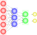
Figure 1: Dynamical Systems Driven by NN Controllers (left) and Nonlinear Feedback System Representation (right).

From the standard $\displaystyle L_{2}$-induced-norm-based small-gain theorem [19], we see that the feedback system shown in Fig. 1 is (well-posed and) globally stable if $\displaystyle\|G\|_{2}<1$. On the other hand, by actively using the nonnegative nature of $\displaystyle\Phi$, it has been shown recently in [23] that the feedback system is (well-posed and) globally stable if $\displaystyle\|G\|_{2+}<1$. As illustrated by this concrete example, the $\displaystyle L_{2+}$-induced-norm-based small-gain theorem has potential abilities for the stability analysis of feedback systems with nonnegative nonlinearities. However, exact computation of the $\displaystyle L_{2+}$ induced norm is inherently difficult and this strongly motivates the current study on its upper and lower bounds computation. The signal-nonnegativity-based analysis of NNs can also be found at [16].

2.3 Problem Settings

This subsection poses three problems to be investigated in this paper. Since the (upper bound of) $\displaystyle L_{2+}$ induced norm is of premier importance as illustrated in Subsection 2.2, we naturally consider the next problem.

Problem 1 ($\displaystyle L_{2+}$ Upper Bound Analysis).

For a given stable LTI system $\displaystyle G$ of the form (1), find an upper bound of $\displaystyle\|G\|_{2+}$ that is as small as possible.

On the other hand, $\displaystyle\|G\|_{p+}\leq\|G\|_{p}$ does hold for $\displaystyle p\in[1,\infty)$ and $\displaystyle p=\infty$. On this relationship, we are interested in how far $\displaystyle\|G\|_{p+}$ can be smaller than $\displaystyle\|G\|_{p}$. To clarify this point, we investigate the next problem.

Problem 2 (Uniform Lower Bound Analysis).

For each $\displaystyle p\in[1,\infty)$ and $\displaystyle p=\infty$, find the uniform lower bound $\displaystyle\nu_{p}^{\star}$ defined by

$$\nu_{p}^{\star}:=\sup\left\{\nu_{p}\in{\mathbb{R}}:\ \|G\|_{p+}\geq\nu_{p}\|G\|_{p}\ \forall G\in{{\mathcal{G}}_{\mathrm{LTI}}}\right\}.$$ (3)

Here, $\displaystyle{{\mathcal{G}}_{\mathrm{LTI}}}$ stands for the set of stable and causal LTI systems including infinite dimensional ones.

Remark 1.

We can also characterize $\displaystyle\nu_{p}^{\star}$ by $\displaystyle\nu_{p}^{\star}=\inf_{G\in{{\mathcal{G}}_{\mathrm{LTI}}}}\dfrac{\|G\|_{p+}}{\|G\|_{p}}$. In our main result (Theorem 13), we concretely construct LTI systems that attain this infimum.

Problem 2 deals with a uniform lower bound that is valid for any $\displaystyle G\in{{\mathcal{G}}_{\mathrm{LTI}}}$. However, for each $\displaystyle G\in{{\mathcal{G}}_{\mathrm{LTI}}}$, it is expected that we can obtain better (larger) lower bounds than the uniform one. Such a lower bound for the $\displaystyle L_{2+}$ induced norm is desirable to evaluate the accuracy of the upper bound obtained for Problem 1. Therefore we consider the next problem.

Problem 3 ($\displaystyle L_{2+}$ Lower Bound Analysis).

For a given stable LTI system $\displaystyle G$ of the form (1), find a lower bound of $\displaystyle\|G\|_{2+}$ that is as large as possible.

2.4 Novel Aspects Over [8, 10]

The novel aspects of the present paper over our preceding studies in [8, 10] are summarized as follows:

• Problem 1 is dealt with in [8]. However, one of the key results in [8], i.e., the construction of the monotonically non-increasing sequence of the upper bounds (Theorem 2 in this paper), is given without any proof. The explicit proof is now given in Section 3, thereby the proposed upper bound computation method is completed for the first time in this paper.

• Problem 3 is investigated in [10]. It is nonetheless true that the results there are restricted to be single-input systems due to technical difficulties. In the present paper we succeed in extending the results to multi-input systems (Theorem 6). As a byproduct of the careful treatments of multi-input systems, we are able to derive an intriguing result that could be regarded as an extension of Perron-Frobenius theorem [1] for nonnegative matrices to general (sign-indefinite) matrices (Theorem 40). See Section 6.

• The effectiveness of the upper bound computation method for Problem 1 and the lower bound computation method for Problem 3 is illustrated for multi-input systems in Subsection 6.5. In particular, we provide an interesting numerical example on the evaluation of the difference of positive systems.

On the other hand, explicit results to Problem 2, together with complete proofs for them, are given in [10]. Still, those results are of great importance and also indispensable to streamline the discussion in this paper. We therefore recall the results of [10] in Theorem 13 of Section 4, with minimum remarks on how the main results to Problem 2 have been obtained.

3 Main Results for $\displaystyle L_{2+}$ Upper Bound Analysis Problem

3.1 Upper Bound Computation of $\displaystyle L_{2+}$ Induced Norm by Positive Filters

Let us focus on the case where $\displaystyle G$ in (1) is a finite-dimensional LTI system given by (2) where $\displaystyle x(0)=0$. We assume that the system $\displaystyle G$ is stable, i.e., $\displaystyle A\in{\mathbb{H}}^{n}$. As noted previously, it is very clear that $\displaystyle\|G\|_{2+}\leq\|G\|_{2}$, i.e., $\displaystyle\|G\|_{2}$ is a trivial upper bound of $\displaystyle\|G\|_{2+}$.

For better upper bound computation of $\displaystyle\|G\|_{2+}$, it is promising to actively use the fact that the input signal $\displaystyle w$ is restricted to be nonnegative. To this end, let us introduce the positive filter given by

$$G_{p}:\begin{cases}\dot{x}_{p}(t)=A_{p}x_{p}(t)+B_{p}w(t),\ x_{p}(0)=0,\\ z_{p}(t)=\left[\begin{array}[]{c}I_{{n_{p}}}\\ 0_{{n_{w}},{n_{p}}}\end{array}\right]x_{p}(t)+\left[\begin{array}[]{c}0_{{n_{p}},{n_{w}}}\\ I_{{n_{w}}}\\ \end{array}\right]w(t)\end{cases}$$ (4)

where $\displaystyle A_{p}\in{\mathbb{H}}^{{n_{p}}}\cap{\mathbb{M}}^{{n_{p}}}$, $\displaystyle B_{p}\in{\mathbb{R}}_{+}^{{n_{p}}\times{n_{w}}}$. It is clear that the filter $\displaystyle G_{p}$ is internally positive from Proposition 1.

We next connect the filter $\displaystyle G_{p}$ with $\displaystyle G$ and construct the augmented system $\displaystyle G_{a}$ given by

In the above augmented system $\displaystyle G_{a}$, it is very important to note that the output $\displaystyle z_{p}$ is nonnegative for any nonnegative input $\displaystyle w$. By focusing on this nonnegative property, the next result has been obtained in [8].

Theorem 1 ([8]).

For the LTI system $\displaystyle G$ given by (1) and a given $\displaystyle\gamma>0$, we have $\displaystyle\|G\|_{2+}\leq\gamma$ if there exist $\displaystyle P_{a}\in{\mathbb{S}}^{n+{n_{p}}}$ and $\displaystyle Q_{a}\in{\mathcal{COP}}^{{n_{p}}+{n_{w}}}$ such that

$$\begin{array}[]{@{}l}\begin{bmatrix}P_{a}A_{a}+A_{a}^{T}P_{a}+C_{a}^{T}C_{a}&P_{a}B_{a}+C_{a}^{T}D_{a}\\ B_{a}^{T}P_{a}+D_{a}^{T}C_{a}&D_{a}^{T}D_{a}-\gamma^{2}I_{{n_{w}}}\end{bmatrix}\\ +\begin{bmatrix}0_{n,{n_{p}}+{n_{w}}}\\ I_{{n_{p}}+{n_{w}}}\end{bmatrix}Q_{a}\begin{bmatrix}0_{n,{n_{p}}+{n_{w}}}\\ I_{{n_{p}}+{n_{w}}}\end{bmatrix}^{T}\preceq 0.\end{array}$$ (6)

On the basis of Theorem 6, let us consider the following COP and SDP:

Then, we readily obtain $\displaystyle\|G\|_{2+}\leq\overline{\gamma}_{a}\leq\overline{\overline{\gamma}}_{a}$. Moreover, it is shown in [8] that, for any positive filter $\displaystyle G_{p}$, the corresponding upper bound $\displaystyle\overline{\gamma}_{a}$ satisfies $\displaystyle\overline{\gamma}_{a}\leq\overline{\gamma}\leq\|G\|_{2}$ where $\displaystyle\overline{\gamma}$ is the COP-based filter-free upper bound that is easily deduced from (7) and given explicitly in [8]. Similarly for $\displaystyle\overline{\overline{\gamma}}_{a}$, i.e., $\displaystyle\overline{\overline{\gamma}}_{a}\leq\overline{\overline{\gamma}}\leq\|G\|_{2}$ holds. The matrix $\displaystyle Q_{a}$ captures the nonnegativity of the input and filtered signals and is referred to as the copositive multiplier.

3.2 Concrete Construction of Positive Filters

As for the positive filter $\displaystyle G_{p}$ given by (4), we propose to use the specific form given by

where $\displaystyle\alpha<0$. By increasing the degree $\displaystyle N$ of the positive filter $\displaystyle G_{p}$ given by (4) and (9), we can construct a sequence of COPs in the form of (7) and SDPs in the form of (8). In the following, we denote by $\displaystyle\overline{\gamma}_{a,\alpha,N}$ and $\displaystyle\overline{\overline{\gamma}}_{a,\alpha,N}$ the optimal values of these COPs and SDPs, respectively. In addition, we denote by $\displaystyle A_{a,\alpha,N}$, $\displaystyle B_{a,N}$, $\displaystyle C_{a,N}$, and $\displaystyle D_{a,N}(=D)$ the coefficient matrices of the augmented system $\displaystyle G_{a}$ given by (5) corresponding to the filter of degree $\displaystyle N$. Then, regarding the effectiveness of employing higher-degree positive filters in improving upper bounds, we can obtain the next result.

Theorem 2.

Let us consider the upper bounds of $\displaystyle\|G\|_{2+}$ given by $\displaystyle\overline{\gamma}_{a,\alpha,N}$ and $\displaystyle\overline{\overline{\gamma}}_{a,\alpha,N}$ that are characterized respectively by (7) and (8) with the positive filter $\displaystyle G_{p}$ of the form (4) and (9) of degree $\displaystyle N$. Then, for $\displaystyle N_{1}\leq N_{2}$, we have $\displaystyle\overline{\gamma}_{a,\alpha,N_{2}}\leq\overline{\gamma}_{a,\alpha,N_{1}}$ and $\displaystyle\overline{\overline{\gamma}}_{a,\alpha,N_{2}}\leq\overline{\overline{\gamma}}_{a,\alpha,N_{1}}$.

Proof of Theorem 2: In the following, we prove $\displaystyle\overline{\gamma}_{a,\alpha,N_{2}}\leq\overline{\gamma}_{a,\alpha,N_{1}}$. The proof for $\displaystyle\overline{\overline{\gamma}}_{a,\alpha,N_{2}}\leq\overline{\overline{\gamma}}_{a,\alpha,N_{1}}$ follows similarly. To prove $\displaystyle\overline{\gamma}_{a,\alpha,N_{2}}\leq\overline{\gamma}_{a,\alpha,N_{1}}$, it suffices to show that $\displaystyle\overline{\gamma}_{a,\alpha,N+1}\leq\overline{\gamma}_{a,\alpha,N}$ holds for any $\displaystyle N$. Furthermore, this can be verified by proving that (6) corresponding to the filter of degree $\displaystyle N+1$ holds with $\displaystyle\gamma=\overline{\gamma}_{a,\alpha,N}+\varepsilon$ for any $\displaystyle\varepsilon>0$.

To this end, we first note from the definition of $\displaystyle\overline{\gamma}_{a,\alpha,N}$ that for any $\displaystyle\varepsilon>0$ there exist $\displaystyle P_{a}=P_{a,\alpha,N}\in{\mathbb{S}}^{n+N{n_{w}}}$ and $\displaystyle Q_{a}=Q_{a,\alpha,N}\in{\mathcal{COP}}^{(N+1){n_{w}}}$ such that

To proceed, define $\displaystyle F_{N}:=\begin{bmatrix}I_{{n_{w}}}&0_{{n_{w}},(N-1){n_{w}}}\end{bmatrix}\in{\mathbb{R}}^{{n_{w}}\times N{n_{w}}}$. Then, there exist $\displaystyle\varepsilon_{1},\varepsilon_{2}>0$ such that

where $\displaystyle P_{p}\in{\mathbb{S}}_{++}^{{n_{p}}}$ is the unique solution of the Lyapunov equation $\displaystyle P_{p}A_{p}+A_{p}^{T}P_{p}+I_{Nnw}=0$. By summing up the above inequality with (10) and applying the Schur complement argument, we obtain

Here,

Then, (11) shows that (6) corresponding to the filter of degree $\displaystyle N+1$ holds with $\displaystyle\gamma=\overline{\gamma}_{a,\alpha,N}+\varepsilon$ and

This completes the proof.   

Remark 2.

From Theorem 2, we see that we can construct a monotonically non-increasing sequence of upper bounds $\displaystyle\{\overline{\overline{\gamma}}_{a,\alpha,N}\}$ of $\displaystyle\|G\|_{2+}$ by increasing the degree $\displaystyle N$ and solving the corresponding SDP (8). Of course this is done at the expense of increased computational burden.

Numerical examples on the illustration of the $\displaystyle L_{2+}$ upper bound computation method are given in Subsection 6.5, together with the illustration of the $\displaystyle L_{2+}$ lower bound computation method developed in Section 6.

4 Main Results for Uniform Lower Bound Analysis Problem

The next theorem provides our main results for Problem 2: the uniform lower bound analysis problem.

Theorem 3 ([10]).

For $\displaystyle p\in[1,\infty)$ and $\displaystyle p=\infty$, the uniform lower bounds $\displaystyle\nu_{p}^{\star}$ defined by (3) are given by

$$\nu_{p}^{\star}=2^{\frac{1-p}{p}}\ (p\in[1,\infty)),\quad\nu_{\infty}^{\star}=\frac{1}{2}.$$ (12)

Moreover, the stable LTI system $\displaystyle G^{\star}(s)=1-e^{-Ls}\ (L>0)$ attains

$$\|G^{\star}\|_{p+}=\nu_{p}^{\star}\|G^{\star}\|_{p}\ (p\in[1,\infty),\ p=\infty).$$ (13)

A detailed proof of Theorem 13 is given in [10]. Still the core of the proof can be grasped by simply relying on the linearity of the system $\displaystyle G$ and a convex property of the $\displaystyle L_{p}$ norms of signals as summarized in the following.

For $\displaystyle w\in L_{p}\ (p\in[1,\infty),p=\infty)$ with $\displaystyle\|w\|_{p}=1$, let us define $\displaystyle w_{+},w_{-}\in L_{p+}$ such that $\displaystyle w=w_{+}-w_{-}$ by $\displaystyle w_{+}(t)=\max(w(t),0_{{n_{w}}})$, $\displaystyle w_{-}(t)=\max(-w(t),0_{{n_{w}}})\ (t\in[0,\infty))$. Then, for $\displaystyle p\in[1,\infty)$ and $\displaystyle p=\infty$, we have

$$\begin{array}[]{@{}lcl}\|Gw\|_{p}&=&\|Gw_{+}-Gw_{-}\|_{p}\\ &\leq&\|Gw_{+}\|_{p}+\|Gw_{-}\|_{p}\\ &\leq&\|G\|_{p+}\|w_{+}\|_{p}+\|G\|_{p+}\|w_{-}\|_{p}\\ &=&\|G\|_{p+}(\|w_{+}\|_{p}+\|w_{-}\|_{p})\end{array}$$ (14)

where we used the linearity of the system $\displaystyle G$ in ensuring the first equality. Then, since the function $\displaystyle f(x)=x^{p}\ (p\in[1,\infty))$ is convex for $\displaystyle x\in{\mathbb{R}}_{+}$, and since $\displaystyle\|w_{+}\|_{p}^{p}+\|w_{-}\|_{p}^{p}=1$ by construction, we see that

$$\left(\frac{\|w_{+}\|_{p}+\|w_{-}\|_{p}}{2}\right)^{p}\leq\frac{\|w_{+}\|_{p}^{p}+\|w_{-}\|_{p}^{p}}{2}=\frac{1}{2}$$

and hence

$$\|w_{+}\|_{p}+\|w_{-}\|_{p}\leq 2^{\frac{p-1}{p}}\ (p=[1,\infty)).$$ (15)

On the other hand, it is obvious that

$$\|w_{+}\|_{\infty}+\|w_{-}\|_{\infty}\leq 2.$$ (16)

From (14), (15), and (16), we see that

$$\|G\|_{p+}\geq\nu_{p}^{\star}\|G\|_{p}\ \forall G\in{{\mathcal{G}}_{\mathrm{LTI}}}\ (p=[1,\infty),p=\infty)$$ (17)

where $\displaystyle\nu_{p}^{\star}\ (p=[1,\infty),p=\infty)$ is given in (12). Then, the proof of Theorem 13 can be completed by showing (13), and this has been done in [10]. We emphasize that, since we only rely on the linearity of underlying systems and the properties of $\displaystyle L_{p}$ norms of signals in showing (17), Theorem 13 is valid even if we extend the set $\displaystyle{{\mathcal{G}}_{\mathrm{LTI}}}$ in Problem 2 to the set of linear, stable, time-varying, and noncausal systems including infinite dimensional ones.

5 Main Results for $\displaystyle L_{2+}$ Lower Bound Analysis Problem: Single-Input Case

From Theorem 13, we see that $\displaystyle\|G\|_{2+}\geq\frac{1}{\sqrt{2}}\|G\|_{2}\ \forall G\in{{\mathcal{G}}_{\mathrm{LTI}}}$. However, for each system $\displaystyle G\in{{\mathcal{G}}_{\mathrm{LTI}}}$, it is expected that $\displaystyle\|G\|_{2+}$ can be strictly larger than $\displaystyle\frac{1}{\sqrt{2}}\|G\|_{2}$. In fact, the main contributions of this section are as follows:

• For any stable finite-dimensional single-input LTI system $\displaystyle G$, we prove $\displaystyle\|G\|_{2+}>\frac{1}{\sqrt{2}}\|G\|_{2}$.

• For a given stable finite-dimensional single-input LTI system $\displaystyle G$, we provide a method to compute a lower bound that is strictly larger than $\displaystyle\frac{1}{\sqrt{2}}\|G\|_{2}$.

We derive these results by using basics about frequency responses of LTI systems, and reducing the lower bound analysis problem into a semi-infinite programming problem [32]. The treatment of multi-input systems is deferred to the next section. In the following, we denote by $\displaystyle{{\mathcal{G}}_{\mathrm{LTI,SI}}}$ the set of stable and single-input LTI systems including infinite dimensional ones.

5.1 Reduction to Semi-Infinite Programming Problem

We first recall the next very basic result.

Lemma 1.

For given $\displaystyle a_{m}\in{\mathbb{R}}\ (m=0,\cdots,N)$, $\displaystyle\phi_{m}\in{\mathbb{R}}\ (m=1,\cdots,N)$, $\displaystyle\omega>0$, $\displaystyle T=2\pi/\omega$, and $\displaystyle{\mathcal{I}}=[-T/2,T/2]$, we have

For a given $\displaystyle G\in{{\mathcal{G}}_{\mathrm{LTI,SI}}}$, let us inject the nonnegative input signal

$$w_{\omega}^{[N]}(t):=a_{0}+\cos(\omega t)+\sum_{m=2}^{N}a_{m}\cos(m\omega t)\ (t\geq 0)$$ (18)

where we assume that $\displaystyle a_{0},a_{m}\ (m=2,\cdots,N)$ are chosen such that $\displaystyle w_{\omega}^{[N]}(t)\geq 0\ (t\geq 0)$. If we denote by $\displaystyle z_{\omega}^{[N]}$ the corresponding steady-state output, we see from the steady-state analysis of the frequency response and Lemma 1 that

It follows that

This result motivates us to consider the following semi-infinite programming problem:

For each $\displaystyle\gamma_{N}^{\star}$, we see $\displaystyle\|G\|_{2+}\geq\dfrac{1}{\sqrt{\gamma_{N}^{\star}}}\|G\|_{2}\ (\forall G\in{{\mathcal{G}}_{\mathrm{LTI,SI}}})$. In addition, since $\displaystyle\gamma_{N}^{\star}$ is monotonically non-increasing with respect to $\displaystyle N\in{\mathbb{N}}$, and since $\displaystyle\gamma_{N}^{\star}\geq 1\ (\forall N\in{\mathbb{N}})$ holds, the sequence $\displaystyle\{\gamma_{N}^{\star}\}$ converges. If we define $\displaystyle\gamma^{\star}:=\lim_{N\to\infty}\gamma_{N}^{\star}$, we readily obtain

$$\|G\|_{2+}\geq\dfrac{1}{\sqrt{\gamma^{\star}}}\|G\|_{2}\ \forall G\in{{\mathcal{G}}_{\mathrm{LTI,SI}}}.$$ (22)

5.2 Effective Lower Bound Computation Methods

From Theorem 13, we know that $\displaystyle\|G^{\star}\|_{2+}=\frac{1}{\sqrt{2}}\|G^{\star}\|_{2}$ and hence $\displaystyle\gamma^{\star}\geq 2$ should hold in (22). Therefore, if we are able to construct $\displaystyle w(t)$ such that

then this is an optimal solution for the semi-infinite programming problem (21) in the limit case $\displaystyle N\to\infty$. With this fact in mind, let us consider the nonnegative signal

$$\begin{array}[]{@{}l}w^{\star}(t):=\max(2\cos(t),0)\ (t\geq 0)\end{array}$$ (24)

whose Fourier series expansion is given by

In (21), this corresponds to the case where

From Parseval’s identity, we readily see that

It follows that the signal $\displaystyle w^{\star}$ given by (24) satisfies the optimality condition (23) and hence is an optimal solution for the semi-infinite programming problem (21) in the limit case $\displaystyle N\to\infty$. From these results, we see that the next result holds for any $\displaystyle G\in{{\mathcal{G}}_{\mathrm{LTI,SI}}}$:

This expression leads us to the next results.

Theorem 4.

Suppose $\displaystyle G\in{{\mathcal{G}}_{\mathrm{LTI,SI}}}$ is finite-dimensional. Then, we have $\displaystyle\|G\|_{2+}>\frac{1}{\sqrt{2}}\|G\|_{2}$. In particular, if $\displaystyle\|G\|_{2}=\|G(0)\|_{2}$ holds, then $\displaystyle\|G\|_{2+}=\|G\|_{2}$ holds.

Proof of Theorem 4: We consider the following three cases: (i) $\displaystyle\|G\|_{2}$ is attained at the angular frequency $\displaystyle\omega=0$, i.e., $\displaystyle\|G\|_{2}=|G(0)|_{2}$; (ii) $\displaystyle\|G\|_{2}$ is given as $\displaystyle\|G\|_{2}=|G(j\infty)|_{2}$ where $\displaystyle G(j\infty):=\lim_{\omega\to\infty}G(j\omega)$; (iii) $\displaystyle\|G\|_{2}$ is attained at $\displaystyle\omega=\omega^{\star}\in(0,\infty)$, i.e., $\displaystyle\|G\|_{2}=|G(j\omega^{\star})|_{2}$.

(i) Suppose $\displaystyle\|G\|_{2}=|G(0)|_{2}$. Then, by letting $\displaystyle\omega\to 0$ in (28), we see from (27) that $\displaystyle\|G\|_{2+}\geq|G(0)|_{2}=\|G\|_{2}$. Namely, $\displaystyle\|G\|_{2+}=\|G\|_{2}$ holds.

(ii) Suppose $\displaystyle\|G\|_{2}=|G(j\infty)|_{2}$. Then, we see from (28) and (27) that

(iii) Suppose $\displaystyle\|G\|_{2}=|G(j\omega^{\star})|_{2}\ (\omega^{\star}\in(0,\infty))$. Then, for $\displaystyle\|G\|_{2+}=\frac{1}{\sqrt{2}}\|G\|_{2}$ to hold, we see from (26) and (28) that the system $\displaystyle G$ should satisfy the infinitely many interpolation constraints:

$$G(0)=0,\ G(j2p\omega^{\star})=0\ (p\in{\mathbb{N}}).$$ (30)

This is impossible for the finite-dimensional system $\displaystyle G$ and hence $\displaystyle\|G\|_{2+}>\frac{1}{\sqrt{2}}\|G\|_{2}$.   

Remark 3.

In Theorem 13, we have shown that the infinite-dimensional system $\displaystyle G^{\star}(s)=1-e^{-Ls}\ (L>0)$ satisfies $\displaystyle\|G^{\star}\|_{2+}=\frac{1}{\sqrt{2}}\|G^{\star}\|_{2}$. Therefore, from the proof of Theorem 4, the system $\displaystyle G^{\star}$ should satisfy the infinitely many interpolation constraints (30). Indeed, we see that $\displaystyle\omega^{\star}=\frac{1}{L}\pi$ for $\displaystyle G^{\star}$, and $\displaystyle G^{\star}$ does satisfy the interpolation constraints (30) since $\displaystyle G^{\star}(0)=0$, and $\displaystyle G^{\star}(j2p\omega^{\star})=0\ (p\in{\mathbb{N}})$.

For a given system $\displaystyle G\in{{\mathcal{G}}_{\mathrm{LTI,SI}}}$, we finally make active use of (28) for the lower bound computation of $\displaystyle\|G\|_{2+}$. By truncation of the infinite series, let us define

Then, it is straightforward from Theorem 4 that the next results hold.

Theorem 5.

Suppose $\displaystyle G\in{{\mathcal{G}}_{\mathrm{LTI,SI}}}$ is finite-dimensional and define $\displaystyle\upsilon_{N}(G)\ (N\in{\mathbb{N}})$ by (31). Then, we have

$$\|G\|_{2+}\geq\upsilon_{N}(G)\geq\frac{1}{\sqrt{2}}\|G\|_{2}\ (\forall N\in{\mathbb{N}}).$$

In particular, $\displaystyle\upsilon_{N}(G)$ is monotonically non-decreasing with respect to $\displaystyle N\in{\mathbb{N}}$, and for sufficiently large $\displaystyle N$ we have $\displaystyle\upsilon_{N}(G)>\frac{1}{\sqrt{2}}\|G\|_{2}$.

We finally note that $\displaystyle\upsilon_{N}(G)$ can readily be computed by using (26) in the way that

6 Main Results for $\displaystyle L_{2+}$ Lower Bound Analysis Problem: Multi-Input Case

To see the difference between single-input and multi-input cases, let us consider the “static” multi-input system $\displaystyle G:=[\ 1\ -1\ ]$. Then, we can readily see that $\displaystyle\|G\|_{2}=\sqrt{2}$ and $\displaystyle\|G\|_{2+}=1$. Namely, $\displaystyle\|G\|_{2+}=\frac{1}{\sqrt{2}}\|G\|_{2}$ holds. This example clearly shows that whole assertions in Theorems 4 and 5 do not hold for multi-input systems in general. With this fact in mind, the goal of this section is as follows:

1. For any $\displaystyle G\in{{\mathcal{G}}_{\mathrm{LTI}}}$, we provide a method to compute a lower bound that is larger than or equal to $\displaystyle\frac{1}{\sqrt{2}}\|G\|_{2}$.

2. By numerical examples on a multi-input system $\displaystyle G\in{{\mathcal{G}}_{\mathrm{LTI}}}$, we show that the method can yield lower bounds that are strictly larger than $\displaystyle\frac{1}{\sqrt{2}}\|G\|_{2}$.

On the size of the input and output signals in (1), we remind $\displaystyle w(t)\in{\mathbb{R}}^{{n_{w}}}$ and $\displaystyle z(t)\in{\mathbb{R}}^{{n_{z}}}$.

6.1 The Case $\displaystyle\|G\|_{2}=\|G(j\omega^{\star})\|_{2}\ (\omega^{\star}\in(0,\infty))$

We first consider the case where $\displaystyle\|G\|_{2}=\|G(j\omega^{\star})\|_{2}\ (\omega^{\star}\in(0,\infty))$ holds, i.e., $\displaystyle\|G\|_{2}$ is attained at the angular frequency $\displaystyle\omega=\omega^{\star}\ (\omega^{\star}\in(0,\infty))$. Suppose $\displaystyle v\in{\mathbb{C}}^{{n_{w}}}$ is the unit right singular vector corresponding to the maximum singular value of $\displaystyle G(j\omega^{\star})$. In the following, we represent the $\displaystyle i$-th element of $\displaystyle v$ by $\displaystyle v_{i}=|v_{i}|e^{j\theta_{i}}\ (i=1,\cdots,{n_{w}})$.

Under these notations, let us consider the nonnegative input signal $\displaystyle w^{\star}(t)\in{\mathbb{R}}^{{n_{w}}}$ defined by

$$w_{i}^{\star}(t):=|v_{i}|\times\max(2\cos(\omega^{\star}t+\theta_{i}),0)\ (i=1,\cdots,{n_{w}}).$$ (33)

If we define $\displaystyle v^{[m]}\in{\mathbb{C}}^{{n_{w}}}\ (m=0,1,2\cdots)$ by

$$v_{i}^{[m]}=|v_{i}|e^{jm\theta_{i}}\ (i=1,\cdots,{n_{w}}),$$ (34)

we see from (24), (25), (26) that

$$w^{\star}(t)=\mathrm{Re}(\widehat{w}^{\star}(t)),$$ (35)

$$\widehat{w}^{\star}(t)=a_{0}^{\star}v^{[0]}+v^{[1]}e^{j\omega^{\star}t}+\sum_{m=2}^{\infty}a_{m}^{\star}v^{[m]}e^{jm\omega^{\star}t}.$$

Then, if we define single-input transfer functions by

$$G^{[m]}(s):=G(s)v^{[m]}\ (m=0,1,2\cdots),$$ (36)

we see from the basic property of frequency response of LTI systems that the steady state output $\displaystyle z^{\star}(t)\in{\mathbb{R}}^{{n_{z}}}$, corresponding to the input $\displaystyle w^{\star}(t)\in{\mathbb{R}}^{{n_{w}}}$, is given by

We also note that $\displaystyle\|G\|_{2}=\|G(j\omega^{\star})\|_{2}=|G^{[1]}(j\omega^{\star})|_{2}$. Then, for $\displaystyle T=2\pi/\omega^{\star}$ and $\displaystyle{\mathcal{I}}=[-T/2,T/2]$, we have

Motivated by this fact, let us define

Then, it is straightforward from (37) that the next results hold.

Theorem 6.

Suppose $\displaystyle G\in{{\mathcal{G}}_{\mathrm{LTI}}}$ and define $\displaystyle\upsilon_{N}(G)\ (N\in{\mathbb{N}})$ by (38). Then, we have

$$\|G\|_{2+}\geq\upsilon_{N}(G)\geq\frac{1}{\sqrt{2}}\|G\|_{2}\ (\forall N\in{\mathbb{N}}).$$

In particular, $\displaystyle\upsilon_{N}(G)$ is monotonically non-decreasing with respect to $\displaystyle N\in{\mathbb{N}}$.

Remark 4.

In the single-input case (i.e., if $\displaystyle{n_{w}}=1$), it is clear that Theorem 6 reduces to Theorem 5. This is because if $\displaystyle{n_{w}}=1$ then we have $\displaystyle v^{[m]}=1\ (m=0,1,2\cdots)$ and hence $\displaystyle G^{[m]}(s)=G(s)\ (m=0,1,2\cdots)$ hold in (36).

6.2 The Case $\displaystyle\|G\|_{2}=\|G(0)\|_{2}$

We next consider the case where $\displaystyle\|G\|_{2}=\|G(0)\|_{2}$ holds, i.e., $\displaystyle\|G\|_{2}$ is attained at the angular frequency $\displaystyle\omega=0$. We cannot simply apply the method in the preceding subsection to $\displaystyle\omega^{\star}=0$, since our underlying result, Lemma 1, never holds for $\displaystyle\omega=0$. Similarly to the single-input case, such a discussion to take the limit $\displaystyle\omega^{\star}\to 0$ might be plausible, but we encounter a difficulty since, as shown in (34), the method in the preceding subsection requires an explicit representation of the unit right singular vector corresponding to the maximum singular value of $\displaystyle G(j\omega^{\star})$ (this is not the case for single-input case). On the basis of these observations, here we first blindly follow the discussion in the preceding subsection applied to $\displaystyle\omega^{\star}=0$, and validate the obtained results directly later on.

Suppose $\displaystyle v\in{\mathbb{R}}^{{n_{w}}}$ is the unit right singular vector corresponding to the maximum singular value of the matrix $\displaystyle G(0)\in{\mathbb{R}}^{{n_{z}}\times{n_{w}}}$. We define $\displaystyle v_{+}=\max(v,0)$ and $\displaystyle v_{-}=-\max(-v,0)$. Then, we see that $\displaystyle w^{\star}$ defined by (33), corresponding to $\displaystyle\omega^{\star}=0$, becomes $\displaystyle w^{\star}(t)=2v_{+}$ where $\displaystyle\theta_{i}\ (i=1,\cdots,{n_{w}})$ in (33) are $\displaystyle 0$ or $\displaystyle\pi$. We also note that $\displaystyle w^{\star}$ given above can be rewritten as $\displaystyle w^{\star}(t)=v+{v_{\mathrm{abs}}}$ where $\displaystyle v_{\mathrm{abs},i}=|v_{i}|\ (i=1,\cdots,{n_{w}})$. On the other hand, we see that $\displaystyle v^{[m]}\ (m=0,1,2,\cdots)$ defined by (34) become

$$v^{[m]}=\left\{\begin{array}[]{ll}v&m\ \mbox{is odd},\\ {v_{\mathrm{abs}}}&m\ \mbox{is even}.\\ \end{array}\right.$$ (39)

Then, the inequality (37) reduces to

where we used (26), (27), and (39). Since $\displaystyle\|G\|_{2+}\geq\|G(0)\|_{2+}$ obviously holds, it follows that if we are able to directly validate

$$\|G(0)\|_{2+}\geq\dfrac{1}{\sqrt{2}}\sqrt{\|G(0)\|_{2}^{2}+|G(0){v_{\mathrm{abs}}}|_{2}^{2}}$$

for $\displaystyle G(0)\in{\mathbb{R}}^{{n_{z}}\times{n_{w}}}$, then we arrive at the conclusion that all of the results in the preceding subsection are valid even for $\displaystyle\omega^{\star}=0$. This validation is indeed possible as we see in the next theorem.

Theorem 7.

For a given $\displaystyle M\in{\mathbb{R}}^{n\times m}$, suppose $\displaystyle v\in{\mathbb{R}}^{m}$ is the unit right singular vector corresponding to the maximal singular value of $\displaystyle M$. Let us define $\displaystyle{v_{\mathrm{abs}}}\in{\mathbb{R}}^{m}_{+}$ by $\displaystyle v_{\mathrm{abs},i}=|v_{i}|\ (i=1,\cdots,m)$. Then, we have

$$\|M\|_{2+}\geq\frac{1}{\sqrt{2}}\sqrt{\|M\|_{2}^{2}+|M{v_{\mathrm{abs}}}|_{2}^{2}}.$$ (40)

Proof of Theorem 40: Without loss of generality, we choose (the sign of) $\displaystyle v$ such that $\displaystyle|v_{+}|_{2}\geq|v_{-}|_{2}$ where $\displaystyle v_{+}=\max(v,0)$ and $\displaystyle v_{-}=-\max(-v,0)$. To prove (40), it suffices to show that

$$\dfrac{|Mv_{+}|_{2}}{|v_{+}|_{2}}=\dfrac{|M(v+{v_{\mathrm{abs}}})|_{2}}{|v+{v_{\mathrm{abs}}}|_{2}}\geq\frac{1}{\sqrt{2}}\sqrt{\|M\|_{2}^{2}+|M{v_{\mathrm{abs}}}|_{2}^{2}}$$

or equivalently,

$$|M(v+{v_{\mathrm{abs}}})|_{2}\geq\frac{1}{\sqrt{2}}|v+{v_{\mathrm{abs}}}|_{2}\sqrt{\|M\|_{2}^{2}+|M{v_{\mathrm{abs}}}|_{2}^{2}}.$$

Since $\displaystyle v^{T}{v_{\mathrm{abs}}}=|v_{+}|_{2}^{2}-|v_{-}|_{2}^{2}(\geq 0)$ holds, we obtain

$$|M(v+{v_{\mathrm{abs}}})|_{2}^{2}=\|M\|_{2}^{2}(1+2(|v_{+}|^{2}-|v_{-}|^{2}))+|M{v_{\mathrm{abs}}}|_{2}^{2}.$$

On the other hand, we have

$$\left(\frac{1}{\sqrt{2}}|v+{v_{\mathrm{abs}}}|_{2}\sqrt{\|M\|_{2}^{2}+|M{v_{\mathrm{abs}}}|_{2}^{2}}\right)^{2}$$

$$=\frac{1}{2}|v+{v_{\mathrm{abs}}}|_{2}^{2}(\|M\|_{2}^{2}+|M{v_{\mathrm{abs}}}|_{2}^{2})$$

$$=(1+|v_{+}|^{2}-|v_{-}|^{2})(\|M\|_{2}^{2}+|M{v_{\mathrm{abs}}}|_{2}^{2}).$$

Therefore we see that

$$|M(v+{v_{\mathrm{abs}}})|_{2}^{2}-\left(\frac{1}{\sqrt{2}}|v+{v_{\mathrm{abs}}}|_{2}\sqrt{\|M\|_{2}^{2}+|M{v_{\mathrm{abs}}}|_{2}^{2}}\right)^{2}$$

$$=(|v_{+}|^{2}-|v_{-}|^{2})\|M\|_{2}^{2}-(|v_{+}|^{2}-|v_{-}|^{2})|M{v_{\mathrm{abs}}}|_{2}^{2}$$

$$=(|v_{+}|^{2}-|v_{-}|^{2})(\|M\|_{2}^{2}-|M{v_{\mathrm{abs}}}|_{2}^{2})\geq 0.$$

This completes the proof.   

Remark 5.

Perron-Frobenius theorem [1] tells us that, for a given nonnegative matrix $\displaystyle M\in{\mathbb{R}}_{+}^{n\times m}$, the unit right singular vector $\displaystyle v\in{\mathbb{R}}^{m}$ corresponding to the maximal singular value is nonnegative, and hence $\displaystyle\|M\|_{2}=\|M\|_{2+}$ holds. The result in Theorem 40 is perfectly consistent with this fact, since if $\displaystyle M\in{\mathbb{R}}_{+}^{n\times m}$ then $\displaystyle{v_{\mathrm{abs}}}=v$ and hence (40) reduces to

$$\|M\|_{2}\geq\|M\|_{2+}\geq \frac{1}{\sqrt{2}}\sqrt{\|M\|_{2}^{2}+|M{v_{\mathrm{abs}}}|_{2}^{2}}$$

$$= \frac{1}{\sqrt{2}}\sqrt{\|M\|_{2}^{2}+\|M\|_{2}^{2}}=\|M\|_{2}.$$

In this sense, we could say that Theorem 40 is a natural extension of the singular value result for nonnegative matrices to general (sign indefinite) matrices.

Remark 6.

From the proof of Theorem 40, we see that

$$\|M\|_{2+}\geq\frac{|Mv_{+}|_{2}}{|v_{+}|_{2}}\geq\frac{1}{\sqrt{2}}\|M\|_{2}.$$

Therefore, we can obtain a lower bound of $\displaystyle\|M\|_{2+}$ that is larger (no smaller) than $\displaystyle\frac{1}{\sqrt{2}}\|M\|_{2}$ by computing $\displaystyle|Mv_{+}|_{2}/|v_{+}|_{2}$.

6.3 The Case $\displaystyle\|G\|_{2}=\|G(\infty)\|_{2}$

We finally consider the case $\displaystyle\|G\|_{2}=\|G(j\infty)\|_{2}$ where $\displaystyle G(j\infty):=\lim_{\omega\to\infty}G(j\omega)$. We assume that $\displaystyle G(j\infty)\in{\mathbb{R}}^{{n_{z}}\times{n_{w}}}$ is well-defined; this is typically the case where $\displaystyle G$ is a finite-dimensional LTI system of the form (2) and in this case we have $\displaystyle G(j\infty)=D\in{\mathbb{R}}^{{n_{z}}\times{n_{w}}}$.

Suppose $\displaystyle v\in{\mathbb{R}}^{{n_{w}}}$ is the unit right singular vector corresponding to the maximum singular value of $\displaystyle G(j\infty)\in{\mathbb{R}}^{{n_{z}}\times{n_{w}}}$. We define $\displaystyle v^{[m]}=v\ (m=0,1,2,\cdots)$ and define $\displaystyle G^{[m]}(s)\ (m=0,1,2,\cdots)$ by (36). Then, it is not hard to see that all the results in Theorem 6 hold. In particular, similarly to (29), we have

6.4 Summary of the Lower Bound Computation

For a given $\displaystyle G\in{{\mathcal{G}}_{\mathrm{LTI}}}$, we now summarize the procedure for the lower bound computation of $\displaystyle\|G\|_{2+}$.

• If $\displaystyle\|G\|_{2}=\|G(j\omega^{\star})\|\ (\omega^{\star}\in[0,\infty))$, denote by $\displaystyle v\in{\mathbb{C}}^{{n_{w}}}$ ($\displaystyle v\in{\mathbb{R}}^{{n_{w}}}$ if $\displaystyle\omega^{\star}=0$) the unit right singular vector corresponding to the maximal singular value of $\displaystyle G(j\omega^{\star})$. Define $\displaystyle v^{[m]}\ (m=0,1,2\cdots)$ by (34). If $\displaystyle\|G\|_{2}=\|G(j\infty)\|$, denote by $\displaystyle v\in{\mathbb{R}}^{{n_{w}}}$ the unit right singular vector corresponding to the maximal singular value of $\displaystyle G(j\infty)\in{\mathbb{R}}^{{n_{z}}\times{n_{w}}}$. Define $\displaystyle v^{[m]}=v\ (m=0,1,2\cdots)$.

• Define $\displaystyle G^{[m]}(s)\ (m=0,1,2\cdots)$ by (36) and compute $\displaystyle\upsilon_{N}(G)$ defined by (38).

Then, as stated in Theorem 6 , we have

$$\|G\|_{2+}\geq\upsilon_{N}(G)\geq\frac{1}{\sqrt{2}}\|G\|_{2}\ (\forall N\in{\mathbb{N}}).$$

In particular, $\displaystyle\upsilon_{N}(G)$ is monotonically non-decreasing with respect to $\displaystyle N\in{\mathbb{N}}$.

Remark 7.

Since $\displaystyle v\in{\mathbb{C}}^{{n_{w}}}$ in general, the transfer functions $\displaystyle G^{[m]}(s)\ (m=0,1,2\cdots)$ in (36) have complex coefficients. Still, the computation of $\displaystyle\upsilon_{N}(G)$ in (38) can be done similarly to (32).

6.5 Numerical Examples

6.5.1 $\displaystyle L_{2+}$ Upper and Lower Bounds Computation

Let us consider the case where the system $\displaystyle G$ in (1) is given by (2) with

In this case, it turned out that $\displaystyle\|G\|_{2}=\|G(j\omega^{\star})\|_{2}=7.0667$ where $\displaystyle\omega^{\star}=0.1654$. We first computed upper bounds of $\displaystyle\|G\|_{2+}$ by following the method in Section 3. The filter-free upper bound turned out to be $\displaystyle 5.3950$. Then, for the poles of the positive filters, we tested the three cases: $\displaystyle\alpha\in\{-0.8,-1.0,-1.2\}$. The results are shown in Fig. 3. The best (least) upper bound with positive filters was $\displaystyle 5.1802\ (\alpha=-0.8,\ N=15)$. With these facts in mind, we next computed $\displaystyle\upsilon_{N}(G)$, the lower bounds of $\displaystyle\|G\|_{2+}$, by following the procedure summarized in the preceding subsection. The results are shown in Fig. 3. The best (largest) lower bound is $\displaystyle 5.1080$. This is indeed larger than $\displaystyle\frac{1}{\sqrt{2}}\|G\|_{2}\approx 4.9967$ obtained from the uniform lower bound shown in Theorem 13. From these upper/lower bounds together with $\displaystyle(5.1802-5.1080)/5.1802\approx 0.0139$, we can conclude that the relative error between the upper bound $\displaystyle 5.1802$ and the true value of $\displaystyle\|G\|_{2+}$ is less than $\displaystyle 1.4\%$.

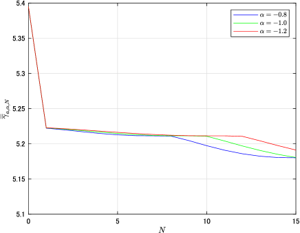
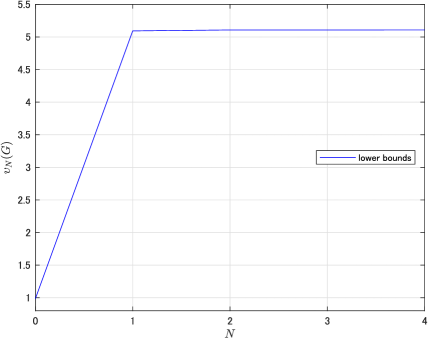
Figure 2: Computed Upper Bounds $\displaystyle\overline{\overline{\gamma}}_{a,\alpha,N}$.

Figure 3: Computed Lower Bounds $\displaystyle\upsilon_{N}(G)$.

6.5.2 Difference of Positive Systems

Let us consider stable and internally (and hence externally) positive systems $\displaystyle G_{1}$, $\displaystyle G_{2}$, $\displaystyle G_{3}$ of the form (2) whose coefficient matrices are

Here, we regard $\displaystyle G_{2}$ and $\displaystyle G_{3}$ of dimension four as reduced order models of $\displaystyle G_{1}$ of dimension six. It turned out that $\displaystyle\|G_{1}-G_{2}\|_{2}=12.43$ and $\displaystyle\|G_{1}-G_{3}\|_{2}=15.69$ and hence we could say that $\displaystyle G_{2}$ is better than $\displaystyle G_{3}$ as a reduced order model in the standard $\displaystyle L_{2}$ induced norm sense. However, since $\displaystyle G_{1}$, $\displaystyle G_{2}$, and $\displaystyle G_{3}$ are all positive, it is more appropriate to compare the closeness in terms of $\displaystyle L_{2+}$ induced norm as stated in Subsection 2.2.1. By the upper bound computation method in Section 3 and the lower bound computation method in Subsection 6.4, we obtained $\displaystyle 12.31\leq\|G_{1}-G_{2}\|_{2+}\leq 12.37$ and $\displaystyle 11.23\leq\|G_{1}-G_{3}\|_{2+}\leq 11.89$. Therefore we are led to the definite conclusion that $\displaystyle G_{3}$ is better than $\displaystyle G_{2}$ as a reduced order model since $\displaystyle\|G_{1}-G_{3}\|_{2+}<\|G_{1}-G_{2}\|_{2+}$. This definite conclusion cannot be obtained unless the proposed upper and lower bounds computation methods.

7 Conclusion

In this paper, we introduced $\displaystyle L_{p+}\ (p\in[1,\infty),p=\infty)$ induced norms for continuous time LTI systems. We first developed an $\displaystyle L_{2+}$ upper bound computation method, we then derived explicit uniform lower bounds of the $\displaystyle L_{p+}$ induced norms with respect to the standard $\displaystyle L_{p}$ induced norms, and finally derived an effective method to compute lower bounds of the $\displaystyle L_{2+}$ induced norm that are better (no smaller) than the uniform one.

From the general integral quadratic constraint framework [22, 31], the COP for the upper bound computation of the $\displaystyle L_{2+}$ induced norm can be regarded as a result that employs copositive multipliers capturing the nonnegativity of the assumed nonlinearities. It is our future topic to clarify the effectiveness of the copositive multipliers in static and dynamical nonlinear system analysis from a broad perspective.

References

- [1] A. Berman and R. J. Plemmons. Nonnegative Matrices in the Mathematical Sciences. SIAM, Philadelphia, New York, San Diego, 1994.
- [2] F. Blanchini, P. Colaneri, and M. E. Valcher. Co-positive Lyapunov functions for the stabilization of positive switched systems. IEEE Transactions on Automatic Control, 57(12):3038–3050, 2012.
- [3] F. Blanchini, P. Colaneri, and M. E. Valcher. Switched positive linear systems. Foundations and Trends® in Systems and Control, 2(2):101–273, 2015.
- [4] C. Briat. Robust stability and stabilization of uncertain linear positive systems via integral linear constraints: -gain and -gain characterization. International Journal of Robust and Nonlinear Control, 23(17):1932–1954, 2013.
- [5] T. Chen, J. B. Lasserre, V. Magron, and E. Pauwels. Semialgebraic optimization for Lipschitz constants of ReLU networks. Advances in Neural Information Processing Systems, 33:19189–19200, 2020.
- [6] C. A. Desoer and M. Vidyasagar. Feedback Systems: Input-Output Properties. Academic Press, New York, 1975.
- [7] M. Dür. Copositive programming - a survey. In M. Diehl, F. Glineur, E. Jarlebring, and W. Michiels, editors, Recent Advances in Optimization and Its Applications in Engineering, pages 3–20. Springer, 2010.
- [8] Y. Ebihara, H. Motooka, H. Waki, N. Sebe, V. Magron, D. Peaucelle, and S. Tarbouriech. induced norm analysis of continuous-time LTI systems using positive filters and copositive programming. In Proc. of the 20th European Control Conference, 2022.
- [9] Y. Ebihara, D. Peaucelle, and D. Arzelier. Analysis and synthesis of interconnected positive systems. IEEE Transactions on Automatic Control, 62(2):652–667, 2017.
- [10] Y. Ebihara, Noboru Sebe, Hayato Waki, and Tomomichi Hagiwara. Lower bound analysis of induced norm for LTI systems. In Proc. the 22th IFAC World Congress, pages 2736–2741, 2023.
- [11] Y. Ebihara, H. Waki, V. Magron, N. H. A. Mai, D. Peaucelle, and S. Tarbouriech. induced norm analysis of discrete-time LTI systems for nonnegative input signals and its application to stability analysis of recurrent neural networks. The 2021 ECC Special Issue of the European Journal of Control, 62:99–104, 2021.
- [12] Y. Ebihara, H. Waki, V. Magron, N. H. A. Mai, D. Peaucelle, and S. Tarbouriech. Stability analysis of recurrent neural networks by IQC with copositive mutipliers. In Proc. of the 60th Conference on Decision and Control, 2021.
- [13] L. Farina and S. Rinaldi. Positive Linear Systems: Theory and Applications. John Wiley and Sons, Inc., 2000.
- [14] M. Fazlyab, M. Morari, and G. J. Pappas. Safety verification and robustness analysis of neural networks via quadratic constraints and semidefinite programming. IEEE Transactions on Automatic Control, 67(1):1–15, 2022.
- [15] M. Fazlyab, A. Robey, H. Hassani, M. Morari, and G. J. Pappas. Efficient and accurate estimation of Lipschitz constants for deep neural networks. In arxiv:1906.04893v2 [cs.LG].
- [16] J. Grönqvist and A. Rantzer. Dissipativity in analysis of neural networks. In Proc. the 25th International Symposium on Mathematical Theory of Networks and Systems, pages 1221–1224, 2022.
- [17] T. Kaczorek. Positive 1D and 2D Systems. Springer, London, 2001.
- [18] T. Kato, Y. Ebihara, and T. Hagiwara. Analysis of positive systems using copositive programming. IEEE Control Systems Letters, 4(2):444–449, 2020.
- [19] H. Khalil. Nonlinear Systems. Prentice Hall, 2002.
- [20] L. Lessard, B. Recht, and A. Packard. Analysis and design of optimization algorithms via integral quadratic constraints. SIAM Journal on Optimization, 26(1):57–95, 2016.
- [21] P. Li, J. Lam, Z. Wang, and P. Date. Positivity-preserving model reduction for positive systems. Automatica, 47(7):1504–1511, 2011.
- [22] A. Megretski and A. Rantzer. System analysis via integral quadratic constraints. IEEE Transactions on Automatic Control, 42(6):819–830, 1997.
- [23] H. Motooka and Y. Ebihara. induced norm analysis for nonnegative input signals and its application to stability analysis of recurrent neural networks (in Japanese). Transactions of the Institute of Systems, Control and Information Engineers, 35(2):29–37, 2022.
- [24] A. Raghunathan, J. Steinhardt, and P. Liang. Certified defenses against adversarial examples. In Proc. the International Conference on Learning Representations, 2018.
- [25] A. Raghunathan, J. Steinhardt, and P. Liang. Semidefinite relaxations for certifying robustness to adversarial examples. Advances in Neural Information Processing Systems, pages 10900–10910, 2018.
- [26] A. Rantzer. Scalable control of positive systems. European Journal of Control, 24(1):72–80, 2015.
- [27] A. Rantzer. On the Kalman-Yakubovich-Popov lemma for positive systems. IEEE Transactions on Automatic Control, 61(5):1346–1349, 2016.
- [28] A. Rantzer and M. E. Valcher. Scalable control of positive systems with applications. Annual Review of Control, Robotics, and Autonomous Systems, 4:319–341, 2021.
- [29] T. Reis and E. Virnik. Positivity preserving model reduction. In Lecture Notes in Control and Information Sciences, pages 131–139. Springer-Verlag, Berlin,Heidelberg, 2009.
- [30] M. Revay, R. Wang, and I. R. Manchester. A convex parameterization of robust recurrent neural networks. IEEE Control Systems Letters, 5(4):1363–1368, 2021.
- [31] C. W. Scherer. Dissipativity and integral quadratic constraints: Tailored computational robustness tests for complex interconnections. IEEE Control Systems Magazine, 42(3):115–139, 2022.
- [32] A. Shapiro. Semi-infinite programming, duality, discretization and optimality conditions. Optimization, 58(2):133–161, 2009.
- [33] A. Sootla and A. Rantzer. Scalable positivity preserving model reduction using linear energy functions. In Proc. Conference on Decision and Control, pages 4285–4290, 2012.
- [34] T. Tanaka and C. Langbort. The bounded real lemma for internally positive systems and structured static state feedback. IEEE Transactions on Automatic Control, 56(9):2218–2223, 2011.
- [35] H. Yin, P. Seiler, and M. Arcak. Stability analysis using quadratic constraints for systems with neural network controllers. IEEE Transactions on Automatic Control, 67(4):1980–1987, 2022.