Federated Unlearning: a Perspective of
Stability and Fairness

Abstract

This paper explores the multifaceted consequences of federated unlearning (FU) with data heterogeneity. We introduce key metrics for FU assessment, concentrating on verification, global stability, and local fairness, and investigate the inherent trade-offs. Furthermore, we formulate the unlearning process with data heterogeneity through an optimization framework. Our key contribution lies in a comprehensive theoretical analysis of the trade-offs in FU and provides insights into data heterogeneity’s impacts on FU. Leveraging these insights, we propose FU mechanisms to manage the trade-offs, guiding further development for FU mechanisms. We empirically validate that our FU mechanisms effectively balance trade-offs, confirming insights derived from our theoretical analysis.

1 Introduction

With the advancement of user data regulations, such as GDPR (Regulation, 2018) and CCPA (Goldman, 2020), the concept of “the right to be forgotten” has gained prominence. It necessitates models’ capability to forget or remove specific training data upon users’ request, which is non-trivial since the models potentially memorize training data. Intuitively, the most straightforward approach is to exactly retrain the model from scratch without the data to be forgotten. However, this method is computationally expensive, especially for large-scale models prevalent in modern applications. As a result, the machine unlearning (MU) paradigm is proposed to efficiently remove data influences from models (Cao & Yang, 2015). The effectiveness of unlearning, measured by verification approaches, requires the unlearning mechanism to closely replicate the results of exact retraining without heavy computational burden.

Federated learning (FL) has gained attention in academia and industry with increased data privacy concerns by allowing distributed clients to collaboratively train a model while keeping the data local (Kairouz et al., 2021). While MU offers strategies for traditional centralized machine learning context, federated unlearning (FU) introduces new challenges due to inherent data heterogeneity and privacy concerns in the federated context (Wang et al., 2023). Recent research of FU, such as Gao et al. (2022); Pan et al. (2023a); Che et al. (2023), mainly focused on verification and efficiency in FU, aligning with the main objectives of MU. However, the inherent data heterogeneity in federated systems introduces new challenges: (i) due to clients’ diverse preferences for the global model, unlearning certain clients could result in une impacts on individuals; (ii) different clients contribute differently to the global model, thus unlearning specific clients can lead to diverse impacts on model performance.

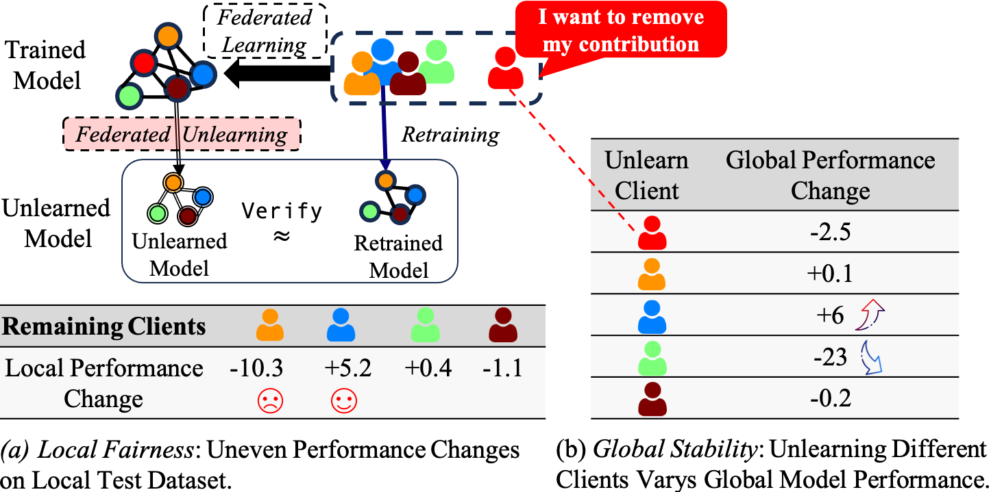
Figure 1: Federated Unlearning and Its Consequences. (a) We consider an FL system of $5$ clients with non-IID training data. One client requests to be unlearned. (b) We conduct $5$ experiments, each featuring the unlearning of one specific client.

On the challenges of FU under heterogeneous data.

Figure 1 elaborates two key insights into the challenges posed by data heterogeneity in FU. (1) Local Fairness: As shown in Figure 1(a), FU can unequally impact remaining clients, where some clients benefit from unlearning, but others experience disadvantages. It illustrates a “local fairness” concern, pertaining to the uniform distribution of utility changes among remaining clients after unlearning. (2) Global Stability: Unlearning different clients leads to different impacts on the global model’s performance, as depicted in Figure 1(b). This highlights the “global stability” concern in FU, emphasizing the need to maintain consistent system performance. These empirical findings identify two trade-offs inherent in FU: the FU verification vs. global stability trade-off, and the FU verification vs. local fairness trade-off. These insights motivate us to ask:

How can we assess the consequences of FU, and what are the theoretical and practical approaches to balancing the inherent trade-offs?

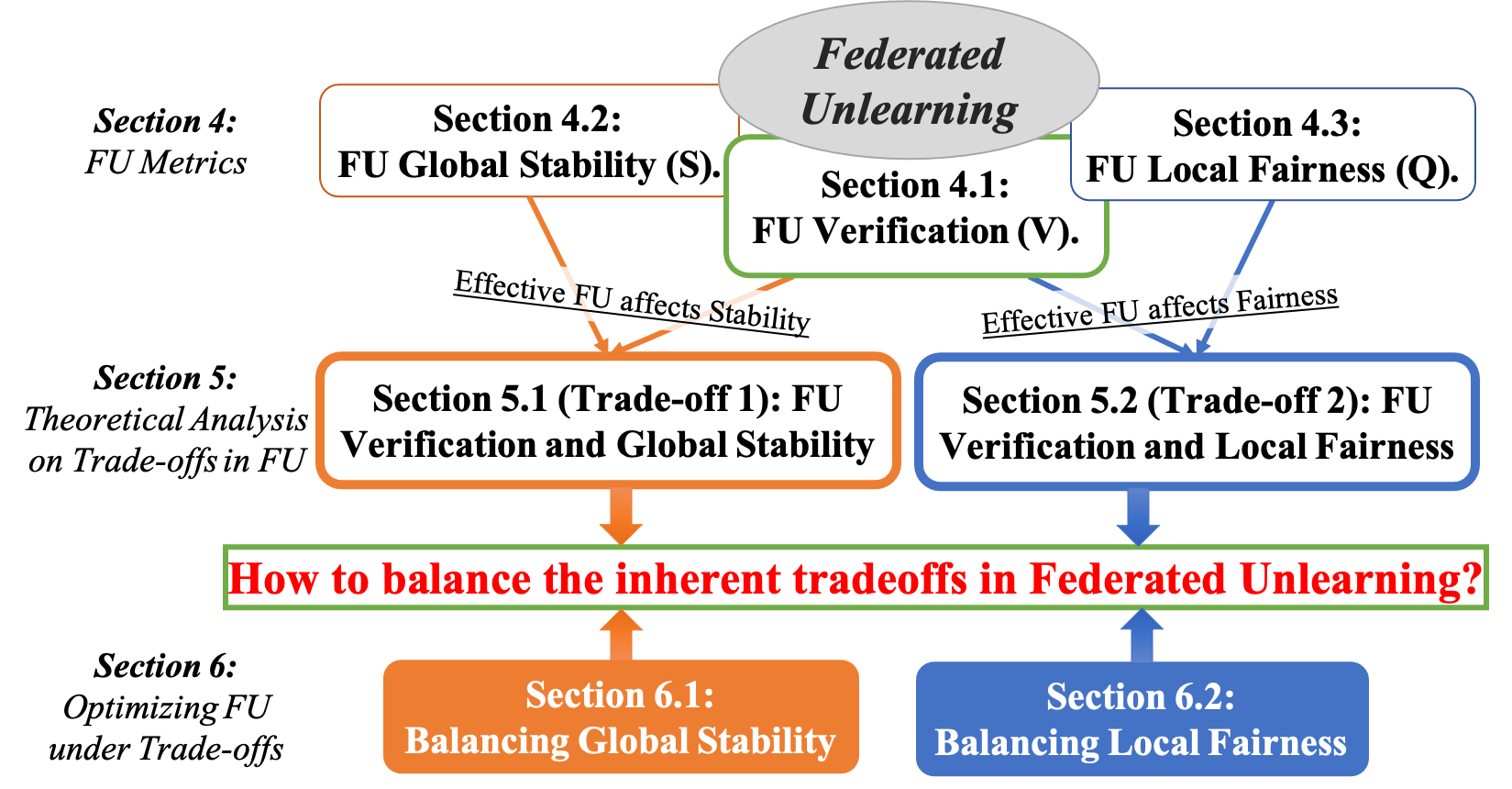
Figure 2: Outline of this paper.

To address the above question, we will construct a comprehensive theoretical framework for FU’s consequences, which should offer a rigorous understanding of how data heterogeneity affects FU while balancing the trade-offs.

Contributions. We outline the structure of our paper in Figure 2 and summarize our key contributions as follows:

1. Quantitative Understanding of FU Metrics: We introduce robust quantitative metrics for FU assessment, including FU verification metric, global stability metric and local fairness metric (detailed in Section 4). These metrics provide a foundation for comprehensive trade-off evaluations in FU.

2. Theoretical Analysis of FU Trade-offs: We present a theoretical analysis of the trade-offs in FU (Section 5). Under data heterogeneity, our results demonstrate challenges in balancing between FU verification and global stability, as well as between FU verification and local fairness.

3. FU Mechanism and Theoretical Framework: We propose a novel FU mechanism based on the theoretical framework, encompassing optimization strategies and penalty methods. We provide the theoretical analysis and practical insights into balancing the tradeoffs within a verifiable FU context, as detailed in Section 6.

4. Empirical Validation: In Section 7, we empirically validate our FU mechanisms in non-convex settings, confirming theoretical insights by effectively balancing trade-offs.

2 Related Work

Mechine Unlearning & Federated Unlearning. Machine unlearning (MU) aims to remove specific data from a machine learning model, addressing the challenges in both effectiveness and efficiency of the unlearning process (Guo et al., 2020; Wu et al., 2020; Bourtoule et al., 2021b; a; Tarun et al., 2023a; b; Jia et al., 2023). In FL, federated unlearning (FU) is proposed to address clients’ right to be forgotten, including methods like rapid retraining (Liu et al., 2022b), subtracting historical updates from the trained model (Wu et al., 2022), subtracting calibrated gradients of the unlearn clients to remove their influence (Liu et al., 2020; 2021), and adding calibrated noises to the trained model by differential privcacy (Zhang et al., 2023). However, none of them involves any rigorous consideration for data heterogeneity, the main challenge in FL. In this work, we account for data heterogeneity in FU through a comprehensive optimization framework, and theoretically analyze how data heterogeneity impacts unlearning in Section 5.

Moreover, existing FU methods has focused on methods ensuring verifiable and efficient unlearning (Liu et al., 2021; 2022b; Fraboni et al., 2022; Gao et al., 2022; Jin et al., 2023; Che et al., 2023). The verification of unlearning typically involves comparing the unlearned model, obtained through an unlearning mechanism, with a reference model using performance metrics such as accuracy and model similarity metrics (Gao et al., 2022). Additionally, attack-based verification methods, such as membership inference attacks (MIA) and backdoor attacks (BA), are often employed in MU (Nguyen et al., 2022) but are not applicable in federated systems due to privacy concerns. Besides verification, data heterogeneity in FU introduces consequences on global stability and local fairness, necessitating consideration of trade-offs in FU, as previously discussed in Section 1. In this work, we conduct a rigorous analysis of inherent trade-offs in FU under data heterogeneity .

Stability in FL and FU. In FL, performance stability revolves around maintaining consistent and robust model performance despite alterations in the training dataset. This aspect of stability, highlighted in studies such as Yin et al. (2018); Fang et al. (2020); Li et al. (2021), often involves defending against external threats. Unlike FL, FU is concerned with managing internal changes within the system for users’ rights to be forgotten (Liu et al., 2022a). Considering unlearning in the federated system, the inherent data heterogeneity can lead to significant shifts in data distribution, thereby altering the model’s performance. In this work, we delve into the theoretical analysis of FU, focusing on examining data heterogeneity’s impacts on stability in FU.

Fairness in FL and FU. In FL, there are several works that have proposed different notions of fairness. The proportional fairness ensures whoever contributes more to the model can gain greater benefits (Wang et al., 2020; Yu et al., 2020). Additionally, the model fairness focuses on protecting specific characteristics, like race and gender (Gu et al., 2022). Furthermore, the performance fairness (Li et al., 2019; Mohri et al., 2019; Hao et al., 2021; Li et al., 2021; Shi et al., 2023; Pan et al., 2023b) aims to reduce the variance of local test performance or utility across all clients.

In FU, we observe that unlearning certain clients can lead to unequal impacts on remaining clients due to data heterogeneity, as discussed in Section 1. In this work, we extend performance fairness to FU by the variance of utility changes among remaining clients and further analyze how data heterogeneity impacts fairness in FU.

3 Preliminaries

3.1 Federated Learning (FL)

Suppose there is a client set $\mathcal{N}$ ($|\mathcal{N}|=N$), contributing to FL training. Each client $i\in\mathcal{N}$ has a local training dataset with size $n_{i}$, and the data is non-IID across different clients. The optimal FL model is defined below:

Definition 3.1 (Optimal FL Model).

The optimal solution of the FL global model, denoted as $\boldsymbol{w}^{*}$, can be expressed by the following optimization problem:

$$\textstyle\boldsymbol{w}^{*}=\arg\min_{\boldsymbol{w}}[F(\boldsymbol{w}):=\sum_{i\in\mathcal{N}}p_{i}f_{i}(\boldsymbol{w})]$$

Here, $f_{i}$ denotes the local objective function of client $i$ with the aggregation weight $p_{i}=\frac{n_{i}}{\sum_{k\in\mathcal{N}}n_{k}}$.

The empirically trained model $\boldsymbol{\boldsymbol{w}}^{o}$ is obtained by training all clients $i\in\mathcal{N}$, serving as the empirical approximation of the theoretical optimum $\boldsymbol{w}^{*}$ (summarized in Figure 3).

3.2 Federated Unlearning (FU)

FU mechanisms aim to obtain an unlearned model $\boldsymbol{{w}}^{u}$ that removes the influence of client set $\mathcal{J}$ who requests to be forgotten from the original trained model $\boldsymbol{\boldsymbol{w}}^{o}$. This paper focuses on the FU mechanism that begins with $\boldsymbol{\boldsymbol{w}}^{o}$ and iteratively updates it through the participation of the remaining clients ($i\notin\mathcal{J}$). The model is refined over $T$ rounds akin to FL, converging to the unlearned model $\boldsymbol{{w}}^{u}$. The optimal unlearned model could be defined as:

Definition 3.2 (Optimal FU Model).

In the context of FU, the optimal unlearned model is defined as the minimizer for the global objective $F_{-\mathcal{J}}$ of all remaining clients $i\notin\mathcal{J}$. Formally, it is expressed as:

$$\textstyle\boldsymbol{w}^{r*}=\arg\min_{\boldsymbol{w}}[F_{-\mathcal{J}}(\boldsymbol{w}):=\sum_{i\notin\mathcal{J}}p_{i}^{\prime}f_{i}(\boldsymbol{w})],$$

Here, $p_{i}^{\prime}$ is the normalized aggregation weight during unlearning, i.e., $p_{i}^{\prime}=\frac{p_{i}}{1-P_{\mathcal{J}}}$ with $P_{\mathcal{J}}=\sum_{j\in\mathcal{J}}p_{j}$.

The exact retrained model $\boldsymbol{w}^{r}$ is obtained after retraining all remaining clients, serving as the empirical approximation of the theoretical optimum $\boldsymbol{w}^{r*}$ (summarized in Figure 3).

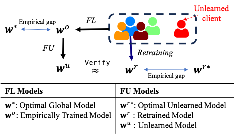
Figure 3: Key Model Notations ($\boldsymbol{{w}}^{u}$ represents the unlearned model from the FU mechanism; $\boldsymbol{w}^{r}$ is from retraining with remaining clients, the special case of $\boldsymbol{{w}}^{u}$).

4 FU Metrics

This section introduces quantitative metrics for evaluating FU mechanisms. In Section 4.1, we elaborate on the verification metric to verify the effectiveness of the FU process. Section 4.2 assesses FU’s impact on the system’s global stability, quantifying how FU alters the global performance of the model. Additionally, Section 4.3 evaluates FU’s impact on local fairness, capturing how FU unequally impacts individuals in remaining clients. These metrics lay the foundation for our comprehensive framework that captures the inherent trade-offs in FU, such as balancing between FU verification and global stability, as well as FU verification and local fairness.

4.1 FU Verification

Verification is critical to evaluate how much the unlearning mechanism effectively removes the data (Yang & Zhao, 2023). Previous studies on unlearning verification often utilize a weak reference like $\boldsymbol{w}^{r}$ from retraining for comparison (Halimi et al., 2022; Che et al., 2023), but this reference is often inconsistent for variability and randomness in the retraining process. Thus, we employ the optimal unlearned model $\boldsymbol{w}^{r*}$ as a theoretical benchmark for verification, allowing for consistent and replicable evaluations in FU. We define a verification metric by the performance gap between the unlearned model and $\boldsymbol{w}^{r*}$:

Definition 4.1 (FU Verification Metric, $V$).

Consider an FU mechanism $\mathcal{M}$ designed to remove specific clients’ influence, resulting in the unlearned model $\boldsymbol{{w}}^{u}$. The unlearning verification metric $V(\boldsymbol{{w}}^{u})$ quantifies the effectiveness of $\mathcal{M}$ and is defined as:

$$V(\boldsymbol{{w}}^{u})=\mathbb{E}\left[F_{-\mathcal{J}}(\boldsymbol{{w}}^{u})\right]-F_{-\mathcal{J}}(\boldsymbol{w}^{r*}),$$ (1)

where $F_{-\mathcal{J}}(\cdot)$ measures performance over the remaining clients after unlearning certain clients set $\mathcal{J}$.

4.2 Global Stability

Effective unlearning often requires modification to the trained model, which can lead to performance variations of the global model. In FL, maintaining stable performance is particularly challenging under data heterogeneity, as unlearning critical clients can significantly compromise model performance. To measure the extent of performance stability in FU, we propose the global stability metric as follows:

Definition 4.2 (Global Stability Metric, $S$).

Given an FU mechanism $\mathcal{M}$ and its resulting unlearned model $\boldsymbol{{w}}^{u}$. The metric $S(\boldsymbol{{w}}^{u})$ evaluates the global stability of $\mathcal{M}$, measuring the performance gap between the unlearned model $\boldsymbol{{w}}^{u}$ and the optimal original FL model $\boldsymbol{w}^{*}$:

$$S(\boldsymbol{{w}}^{u})=\mathbb{E}\left[F(\boldsymbol{{w}}^{u})\right]-F(\boldsymbol{w}^{*}).$$ (2)

This metric $S$ evaluates the stability of the FU process, facilitating understanding of theoretical analysis in Section 5.1.

4.3 Local Fairness

In FL, fairness can be associated with the consistency of model performance across different clients. Specifically, a model is considered fairer if its performance has a smaller variance across clients (Li et al., 2020a).

For FU, effectively unlearning certain clients can unequally impact remaining clients because they have diverse preferences for the global model (data heterogeneity). As demonstrated in Section 1, some clients experience significant utility degradation after unlearning, potentially prompting their departure and further degrading system performance. To measure this FU impact, we propose the local fairness metric as follows:

Definition 4.3 (Local Fairness Metric, $Q$).

Given an FU mechanism $\mathcal{M}$ and its resulting unlearned model $\boldsymbol{{w}}^{u}$. The metric $Q(\boldsymbol{{w}}^{u})$ evaluates local fairness of $\mathcal{M}$, assessing the unequal impact of FU on remaining clients:

$$\textstyle Q(\boldsymbol{{w}}^{u})=\sum_{i\notin\mathcal{J}}p_{i}^{\prime}\left|\Delta f_{i}(\boldsymbol{{w}}^{u})-\overline{\Delta f}\right|,$$ (3)

where $\Delta f_{i}(\boldsymbol{{w}}^{u})=\mathbb{E}\left[f_{i}(\boldsymbol{{w}}^{u})\right]-f_{i}(\boldsymbol{w}^{*})$ represents the utility change for remaining client $i\notin\mathcal{J}$ due to FU. Moreover, $\overline{\Delta f}=\sum_{i\notin\mathcal{J}}p_{i}^{\prime}\Delta f_{i}(\boldsymbol{{w}}^{u})$ is the weighted average of local utility changes among remaining clients, serving as a benchmark for assessing deviation in the impacts of unlearning.

The metric $Q$ is inspired by the mean absolute deviation (MAD) in measuring fairness of FL (Ezzeldin et al., 2023). The metric $Q$ captures FU’s impact on utility changes experienced by remaining clients and further facilitates theoretical analysis of fairness implication in Section 5.2.

5 Theoretical Analysis on Trade-offs in FU

This section provides a theoretical analysis of the trade-offs in FU, particularly focusing on the balance between FU verification and stability, as well as FU verification and fairness, as outlined in Section 5.1 and 5.2, respectively. Our analysis critically examines the challenges posed by data heterogeneity in FU. To begin, we formally state the assumptions required for the theoretical analysis.

Assumption 5.1 (Data Heterogeneity in FL).

Given a subset of remaining clients $\mathcal{S}$, the data heterogeneity among remaining clients can be quantified as follows:

$$\mathbb{E}_{i\in S}\left\|\nabla f_{i}(\boldsymbol{w})-\nabla F_{-\mathcal{J}}(\boldsymbol{w})\right\|^{2}\leq\zeta_{\mathcal{S}}^{2}+\beta_{\mathcal{S}}^{2}\|\nabla F_{-\mathcal{J}}(\boldsymbol{w})\|^{2},$$ (4)

where $\zeta_{\mathcal{S}}^{2}$ and $\beta_{\mathcal{S}}^{2}$ are parameters quantifying the heterogeneity. Here, $f_{i}$ represents the objective function of client $i$ in subset $\mathcal{S}$, and $F_{-\mathcal{J}}$ is the global objective function of the remaining clients.

Assumption 5.2 ($\mu$-strong Convexity).

Let the objective function $f:\mathbb{R}^{d}\rightarrow\mathbb{R}$ be $\mu$-strong convex. For any vectors $\mathbf{u},\mathbf{v}\in\mathbb{R}^{d}$, the function $f$ satisfies the following inequality: $f(\mathbf{u})\geq f(\mathbf{v})+\langle\nabla f(\mathbf{v}),\mathbf{u}-\mathbf{v}\rangle+\frac{\mu}{2}\|\mathbf{u}-\mathbf{v}\|^{2}$, where $\mu>0$ is the convexity constant.

Assumption 5.3 ($L$-smoothness).

Assume that the objective function $f:\mathbb{R}^{d}\rightarrow\mathbb{R}$ is $L$-smooth. For any vectors $\mathbf{u},\mathbf{v}\in\mathbb{R}^{d}$, the function $f$ satisfies the following inequality: $f(\mathbf{u})\leq f(\mathbf{v})+\langle\nabla f(\mathbf{v}),\mathbf{u}-\mathbf{v}\rangle+\frac{L}{2}\|\mathbf{u}-\mathbf{v}\|^{2}$, where $L>0$ is the Lipschitz constant of the gradient of $f$.

Assumption 5.4 (Bounded Variance).

Given a subset of remaining clients $\mathcal{S}$, the aggregation of their stochastic gradients $\boldsymbol{g}_{\mathcal{S}}(\boldsymbol{w})=\sum_{i\in\mathcal{S}}\alpha_{i}\boldsymbol{g}_{i}(\boldsymbol{w})$ is unbiased estimator of $\nabla F_{-\mathcal{J}}(\boldsymbol{w})$ with bounded variance: $\mathbb{E}\left[\left\|\boldsymbol{g}_{\mathcal{S}}(\boldsymbol{w})-\nabla F_{-\mathcal{J}}(\boldsymbol{w})\right\|^{2}\right]\leq\sigma^{2}$.

Assumption 5.5 (Unlearning Clients’ Influence).

Let $P_{\mathcal{J}}$ denote the total aggregation weights of the clients in set $\mathcal{J}$ within FL, defined as $P_{\mathcal{J}}=\sum_{j\in\mathcal{J}}p_{j}$. For a client set $\mathcal{J}$ required for unlearning, we assume that $P_{\mathcal{J}}\leq\frac{1}{2}$.

5.1-5.4 are commonly used for the FL convergence analysis (Li et al., 2020b; Wang et al., 2021). 5.5 assumes unlearned clients’ aggregate weights do not exceed those of the remaining clients. This is crucial to prevent catastrophic consequences, which could undermine the objectives of fairness and stability in FU.

5.1 Trade-off between FU Verification and Stability

This section explores the trade-off between FU verification and global stability via the lower bound derived for verification (Lemma 5.6) and stability (Lemma 5.8). Then, we formalize the trade-off characterized via the lower bounds in Theorem 5.10. We provide all proofs for lemmas and theorems in the Appendix.

Lemma 5.6.

Under Assumptions 5.1-5.4 and given the number of unlearning rounds $T$ and the learning rate $\eta=\frac{1}{T\sqrt{\mu}}\sqrt{\frac{\beta_{\mathcal{S}}-1}{\min\left\{\mu(\beta_{\mathcal{S}}-1),L(\beta_{\mathcal{S}}-1)\right\}}}$, the verification metric $V(\boldsymbol{{w}}^{u})=F_{-\mathcal{J}}(\boldsymbol{{w}}^{u})-F_{-\mathcal{J}}(\boldsymbol{w}^{r*})$ is lower bounded by:

$$C_{1}= \left(1+2\frac{\beta_{\mathcal{S}}^{2}-1}{T}\right)\left(\Delta F_{-\mathcal{J}}\left(\boldsymbol{w}^{*},\boldsymbol{w}^{r*}\right)\right.$$ (5)

$$\left.+\Delta F_{-\mathcal{J}}\left(\boldsymbol{\boldsymbol{w}}^{o},\boldsymbol{w}^{*}\right)\right)+\frac{1}{2LT}\left(\bar{\sigma^{2}}+\bar{\zeta^{2}}\right),$$

where $\Delta F_{-\mathcal{J}}\left(\circ,\bullet\right)=F_{-\mathcal{J}}(\circ)-F_{-\mathcal{J}}(\bullet)$, $\bar{\sigma^{2}}=\frac{1}{T}\sum_{t=1}^{T}\sigma_{t}^{2}$, and $\bar{\zeta^{2}}=\frac{1}{T}\sum_{t=1}^{T}\zeta_{t}^{2}$. Parameters $\beta_{\mathcal{S}}$ and $\bar{\zeta^{2}}$ characterize the data heterogeneity of remaining clients.

Remark 5.7.

The effectiveness of FU, as measured by $V(\boldsymbol{{w}}^{u})$, is hindered by its lower bound $C_{1}$ in Equation 5 with several factors:

• Computational Complexity: More unlearning rounds $T$ typically indicate convergence towards the optimal unlearned model $\boldsymbol{w}^{r*}$, characterized by a tighter lower bound $C_{1}$. However, the computational complexity grows as the number of unlearning rounds $T$ increases.

• Data Heterogeneity among Remaining Clients: A high data heterogeneity ($\beta_{\mathcal{S}}^{2},\bar{\zeta^{2}}^{2}$) among remaining clients can amplify $C_{1}$. Therefore, under unlearning rounds $T$, the more heterogeneous among remaining clients, the more challenging it is to achieve effective unlearning by the increased lower bound $C_{1}$ of $V$.

• Data Heterogeneity Between Remaining and Unlearned Clients: The discrepancy $\Delta F_{-\mathcal{J}}\left(\boldsymbol{w}^{*},\boldsymbol{w}^{r*}\right)$ implies data heterogeneity between remaining and unlearned clients. A high heterogeneity enlarges $C_{1}$, thereby potentially compromising FU verification $V$. Conversely, suppose the data is homogeneous between these two groups, $C_{1}$ can be diminished, as removing homogeneous data does not significantly alter the overall data distribution ($\Delta F_{-\mathcal{J}}\left(\boldsymbol{w}^{*},\boldsymbol{w}^{r*}\right)\approx 0$).

Lemma 5.8.

Under Assumptions 5.2, 5.5 and consider $T\geq\frac{\mu}{\eta^{2}}$ unlearning rounds. The global stability metric $S(\boldsymbol{{w}}^{u})=\mathbb{E}\left[F(\boldsymbol{{w}}^{u})\right]-F(\boldsymbol{w}^{*})$ is bounded below by $C_{2}$:

$$C_{2}=\frac{P_{\mathcal{J}}\eta T}{2}\|\nabla F_{-\mathcal{J}}(\boldsymbol{\boldsymbol{w}}^{o})-\nabla F_{\mathcal{J}}(\boldsymbol{\boldsymbol{w}}^{o})\|^{2}+\delta,$$ (6)

where $\delta=F(\boldsymbol{\boldsymbol{w}}^{o})-F(\boldsymbol{w}^{*})$ represents the empirical risk minimization (ERM) gap in the original FL training.

Remark 5.9.

Maintaining global stability $S(\boldsymbol{{w}}^{u})$ poses challenges due to the lower bound $C_{2}$ established in Equation 6, which is influenced by the following factors:

• Unlearned Clients’ Influence: The higher aggregation weight of unlearned clients $P_{\mathcal{J}}$ implies their substantial influence on the original model. Consequently, their removal has a greater impact on the model’s performance, as reflected by increasing $C_{2}$.

• Data Heterogeneity Between Remaining and Unlearned Clients: $\|\nabla F_{-\mathcal{J}}(\boldsymbol{\boldsymbol{w}}^{o})-\nabla F_{\mathcal{J}}(\boldsymbol{\boldsymbol{w}}^{o})\|^{2}$ measures the objectives divergence between remaining and unlearned clients. A larger value of this term indicates higher heterogeneity between the two groups, contributing to increased $C_{2}$ and thereby increasing instability.

• Unlearning Rounds: Increasing unlearning rounds $T$ can enhance unlearning effectiveness as discussed in Lemma 5.6. However, the growth of $T$, particularly with divergent objectives $\|\nabla F_{-\mathcal{J}}(\boldsymbol{\boldsymbol{w}}^{o})-\nabla F_{\mathcal{J}}(\boldsymbol{\boldsymbol{w}}^{o})\|^{2}$, intensifies instability by increasing $C_{2}$.

Theorem 5.10.

Let Assumptions 5.1-5.5 hold, and given an original trained model $\boldsymbol{\boldsymbol{w}}^{o}$ undergoing unlearning. Consider the learning rate $\eta=\frac{1}{T\sqrt{\mu}}\sqrt{\frac{\beta_{\mathcal{S}}-1}{\min\left\{\mu(\beta_{\mathcal{S}}-1),L(\beta_{\mathcal{S}}-1)\right\}}}$, the sum of the unlearning verification metric and the global stability metric $V(\boldsymbol{{w}}^{u})+S(\boldsymbol{{w}}^{u})$ is bounded below by a constant $C_{s}$, i.e.,

$$C_{s}=\frac{P_{\mathcal{J}}}{\sqrt{2}\mu}\|\nabla F_{-\mathcal{J}}(\boldsymbol{\boldsymbol{w}}^{o})-\nabla F_{\mathcal{J}}(\boldsymbol{\boldsymbol{w}}^{o})\|^{2}+\delta+C_{1},$$ (7)

where $C_{1}$ is defined in Lemma 5.8.

Theorem 5.10 illustrates a fundamental trade-off in FU: effectively unlearning clients ($V$) while maintaining the stability of the global model’s performance ($S$). This trade-off is determined by the divergence between the optimal model $\boldsymbol{w}^{*}$ and the optimal unlearned model $\boldsymbol{w}^{r*}$. Specifically, achieving effective FU and stability is not feasible under the substantial divergence between $\boldsymbol{w}^{*}$ and $\boldsymbol{w}^{r*}$.

5.2 Trade-off between FU Verification and Fairness

This section delves into the trade-off between FU verification and local fairness among the remaining clients. We introduce the following Theorem 5.11, which quantifies this trade-off by a lower bound for the cumulative effect of verification and fairness. The lower bound is determined by the optimality gap, which is defined as the disparity between the performance of the optimal unlearned model $\boldsymbol{w}^{r*}$ and the local optimal models for each remaining client $\boldsymbol{w_{i}}^{*}$.

Theorem 5.11 (Trade-off between Local Fairness and Effective Unlearning).

Within FU, the sum of the unlearning verification metric and the local fairness metric $2V(\boldsymbol{{w}}^{u})+Q(\boldsymbol{{w}}^{u})$ is bounded below by a constant $C_{q}$:

$$\textstyle 2V(\boldsymbol{{w}}^{u})+Q(\boldsymbol{{w}}^{u})\geq C_{q}=F_{-\mathcal{J}}^{*}-\sum_{i\notin\mathcal{J}}p_{i}^{\prime}f_{i}(\boldsymbol{w_{i}}^{*}),$$ (8)

where $\boldsymbol{w_{i}}^{*}$ denotes the local optimal model for client $i$.

Remark 5.12.

The lower bound $C_{q}$ underscores another fundamental trade-off in FU: the balance between effectively unlearning ($V$) and maintaining fairness among the remaining clients ($Q$). If $C_{q}$ is large, optimizing either metric could compromise the other. The challenges of balancing this trade-off primarily arise from data heterogeneity:

• Data Heterogeneity among Remaining Clients: When data distribution is homogeneous among remaining clients, each client’s optimal model ($\boldsymbol{w}_{i}^{*}$ for $\forall i\notin J$) is identical with the optimal unlearned model ($\boldsymbol{w}_{i}^{*}=\boldsymbol{w}^{r*}$). Thus, data homogeneity reduces $C_{q}$ to $0$, indicating FU verification and fairness can be achieved simultaneously. In contrast, higher heterogeneity means divergent optimal models for different clients, thus increasing $C_{q}$ and posing greater challenges in balancing this trade-off.

• Data Heterogeneity Between Remaining and Unlearned Clients: As discussed in Lemma 5.6, a high heterogeneity between remaining and unlearned clients increases lower bound $C_{1}$ for the unlearning verification metric $V$. With a constant $C_{q}$, a larger $V$ typically leads to a reduced fairness metric $Q$. It indicates that under higher heterogeneity, fairness is enhanced for the remaining clients after unlearning. The enhanced fairness is because unlearning divergent clients $\mathcal{J}$ aligns the FU optimal model $\boldsymbol{w}^{r*}$ more closely to remaining clients than the original FL optimal model $\boldsymbol{w}^{*}$. Conversely, under homogeneity between two groups, unlearning reduces $V$ (in Lemma 5.6 $\Delta F_{-\mathcal{J}}\left(\boldsymbol{w}^{*},\boldsymbol{w}^{r*}\right)=0$), and thereby, the fairness metric $Q$ primarily depends on data heterogeneity among remaining clients.

5.3 Trade-off in Verification, Fairness and Stability

As demonstrated in Remark 5.12, given high heterogeneity between remaining and unlearned clients, unlearning can improve fairness for the remaining clients because the FU optimal model more closely aligns with the remaining clients. However, under this heterogeneity, the stability of the federated system is compromised in FU, as discussed in Remark 5.9. This underscores a fundamental trade-off that enhancing fairness compromises the system’s stability. For future work, we will delve into the complex interplay in FU for balancing FU verification, stability, and fairness.

6 Optimizing FU under Trade-offs

In the previous section, we examine the inherent trade-offs involving FU verification and their challenges. To balance these trade-offs, this section introduces our FU mechanisms developed within an optimization framework.

6.1 FU for Balancing Global Stability

In FU, maintaining global stability is crucial for ensuring the overall performance and reliability of the federated system throughout the unlearning process. However, as explored in Section 5.1, a trade-off exists between FU verification and global stability. To manage this trade-off, we propose an FU mechanism utilizing a penalty-based approach and gradient correction techniques. We also theoretically demonstrate the convergence of our method.

FU Mechanism Design: To balance stability during FU, we formulate the optimization problem for unlearning as:

$$\textbf{P1: }\min_{\boldsymbol{w}}V(\boldsymbol{w})+\lambda S(\boldsymbol{w}).$$ (9)

By adjusting $\lambda$, we can manage the trade-off between these two objectives, allowing for a flexible approach to specific requirements of the federated system.

By the definition of stability metric $S(\boldsymbol{w})$, we have: $S(\boldsymbol{w})=\mathbb{E}\left[F(\boldsymbol{w})\right]-F(\boldsymbol{w}^{*})=\mathbb{E}\left[F(\boldsymbol{{w}}^{u})\right]-F(\boldsymbol{\boldsymbol{w}}^{o})+\delta,$ where $\delta=F(\boldsymbol{\boldsymbol{w}}^{o})-F(\boldsymbol{w}^{*})$. Consequently, solving P2: $\min_{\boldsymbol{w}}F_{-\mathcal{J}}(\boldsymbol{w})+\lambda\left(F(\boldsymbol{w})-F(\boldsymbol{\boldsymbol{w}}^{o})\right)$ optimizes P1. However, in P2, optimizing the global objective $F(\boldsymbol{w})$ among all clients is untraceable in FU as it cannot involve unlearned client $j\in\mathcal{J}$ in unlearning process. To address this, we consider the approximate problem P3 to P2:

$$\textstyle\textbf{P3: }\min_{\boldsymbol{w}}H(\boldsymbol{w}):=[F_{-\mathcal{J}}(\boldsymbol{w})+\tilde{h}(\boldsymbol{w})],$$ (10)

where $\tilde{h}(\boldsymbol{w})=(1-P_{\mathcal{J}})F_{1}+P_{\mathcal{J}}F_{2}$, $F_{1}:=\lambda F_{-\mathcal{J}}(\boldsymbol{w})$, and $F_{2}:=\lambda\left(\langle\nabla F_{\mathcal{J}}(\boldsymbol{\boldsymbol{w}}^{o}),\boldsymbol{w}-\boldsymbol{\boldsymbol{w}}^{o}\rangle+\frac{L}{2}\left\|\boldsymbol{w}-\boldsymbol{\boldsymbol{w}}^{o}\right\|^{2}\right)$.

To address P3, we propose an FU mechanism that operates two steps during each unlearning round $t$:

1. Federated Aggregation: The remaining client $i\in\mathcal{S}$ performs local training over $E$ epochs with learning rate $\eta_{l}$ to obtain $\boldsymbol{w}^{(t,E)}_{i}$. Then, the server aggregates $\{\boldsymbol{w}^{(t,E)}_{i}\}_{i\in\mathcal{S}}$ for the global model ${\boldsymbol{\bar{w}}}^{(t,E)}=\sum_{i\in\mathcal{S}}\alpha_{i}\cdot\boldsymbol{w}^{(t,E)}_{i}$, where $\alpha_{i}$ is the weight for client $i$.

2. Global Correction: Following the aggregation, the server applies a gradient correction to ${\boldsymbol{\bar{w}}}^{(t,E)}$. Specially, the server compute $\boldsymbol{h}^{t}=\lambda(1-P_{\mathcal{J}})\boldsymbol{g}_{\mathcal{S}}^{t}+\lambda P_{\mathcal{J}}\boldsymbol{\hat{g}}_{\mathcal{J}}^{t}$, where $\boldsymbol{\hat{g}}_{\mathcal{J}}^{t}(\boldsymbol{w})=\nabla F_{-\mathcal{J}}(\boldsymbol{\boldsymbol{w}}^{o})+L(\boldsymbol{w}-\boldsymbol{\boldsymbol{w}}^{o})$. The correction term $\boldsymbol{g}_{c}^{t}$ is then obtained by projecting $\boldsymbol{h}^{t}$ onto the tangent space of the aggregated gradient $\boldsymbol{g}_{\mathcal{S}}$: $\boldsymbol{g}_{c}^{t}=\boldsymbol{h}^{t}-\text{Proj}_{\boldsymbol{g}_{\mathcal{S}}}\boldsymbol{h}^{t}.$ The global model is updated for the next round: ${\boldsymbol{\bar{w}}}^{(t+1,0)}={\boldsymbol{\bar{w}}}^{(t,E)}-\eta_{g}\boldsymbol{g}_{c}^{t},$ where $\eta_{g}$ is the learning rate for the gradient correction.

The FU mechanism thus iteratively updates the global model by ${\boldsymbol{\bar{w}}}^{(t+1,0)}=\boldsymbol{w}^{(t,0)}-\eta_{l}\boldsymbol{g}_{\mathcal{S}}^{t}-\eta_{g}\boldsymbol{g}_{c}^{t}$.

Theoretical Analysis: Now, we delve into the convergence of the proposed FU mechanism, ensuring its reliability in FU. We also conduct theoretical analysis to determine the upper bound for the verification metric $V$, which is essential for verifying the effectiveness of unlearning. To begin, we formally state the assumptions required for our main results.

Assumption 6.1.

The gradients of local objectives are bounded, i.e., $\|\nabla f_{i}(\boldsymbol{w})\|\leq G$ for all $i$. This implies the gradient of global objective $F_{-\mathcal{J}}$ for remaining clients is also bounded: $\|\nabla F_{-\mathcal{J}}(\boldsymbol{w})\|\leq G$.

Assumption 6.2.

The heterogeneity between the unlearned clients $\mathcal{J}$ and the remaining clients is quantified as:

$${\left\|\mathbb{E}\left[\boldsymbol{\hat{g}}_{\mathcal{J}}^{t}(\boldsymbol{w})\right]-\nabla F_{-\mathcal{J}}(\boldsymbol{w})\right\|^{2}}\leq\zeta^{\prime 2}+\beta^{\prime 2}\left\|\nabla F_{-\mathcal{J}}(\boldsymbol{w})\right\|^{2},$$

where $\boldsymbol{\hat{g}}_{\mathcal{J}}^{t}(\boldsymbol{w})=\nabla F_{-\mathcal{J}}(\boldsymbol{\boldsymbol{w}}^{o})+L(\boldsymbol{w}-\boldsymbol{\boldsymbol{w}}^{o})$, $\zeta^{{}^{\prime}2}$ and $\beta^{{}^{\prime}2}$ indicate heterogeneity between unlearned and remaining clients.

The following lemma derives the upper bound on the expected norm of gradient correction, and then we establish the convergence theorem of our proposed FU mechanism.

Lemma 6.3.

Under 6.2, the expected norm of the gradient correction at unlearning round $t$ is bounded:

$$\mathbb{E}\left[\left\|\boldsymbol{g_{c}}({\boldsymbol{\bar{w}}}^{(t,E)})\right\|^{2}\right]\leq\phi\left(\zeta^{\prime 2}+(\beta^{\prime 2}+1)\left\|\nabla F_{-\mathcal{J}}({\boldsymbol{\bar{w}}}^{t,E})\right\|^{2}\right),$$

where $\phi=\lambda^{2}P_{\mathcal{J}}^{2}(1+\cos^{2}\theta)$, $\cos^{2}\theta$ represents the similarity in objectives between remaining and unlearned clients.

Theorem 6.4 (Convergence).

Let Assumptions 5.1-5.4, 6.1 and 6.2 hold, we consider an FU mechanism with diminishing step size $\eta_{l}=\frac{\beta}{2(t+\gamma)}$ for some $\beta>\frac{1}{\mu}$ and $\gamma>0$, such that $\eta_{l}\leq\frac{1}{4L}$. The convergence result after $t$ rounds is:

$$\mathbb{E}\left[H\left(\bar{\mathbf{w}}^{(t+1,0)}\right)\right]-H\left(\mathbf{w}^{*}\right)\leq\frac{L}{2}\left(\frac{v}{\gamma+t}+\left\|\boldsymbol{w}^{r*}-\boldsymbol{w}^{*}\right\|^{2}\right),$$

where $v=\max\left\{\frac{\beta^{2}B}{\beta\mu-4},(\gamma+1)\left\|\boldsymbol{\boldsymbol{w}}^{o}-\boldsymbol{w}^{r*}\right\|^{2}\right\}$.

Our approach introduces additional complexity in the convergence analysis compared to that of Li et al. (2020b, Theorem 1) due to incorporating a gradient correction in FU, as detailed in Section E.1 This complexity is reflected in $B$ with additional components: $2\phi\left(\frac{\eta_{g}}{\eta_{l}}\right)^{2}((\beta^{\prime 2}+1)G^{2}+\zeta^{\prime 2})$. It highlights two insights:

1. A high data heterogeneity between remaining and unlearned clients, indicated by $\beta^{\prime 2}$ and $\zeta^{\prime 2}$, increases unlearning rounds $T$ for FU convergence;

2. The term $\phi=\lambda^{2}P_{\mathcal{J}}^{2}(1+\cos^{2}\theta)$ in the convergence bound indicates that larger influence of unlearned clients (characterized by $P_{\mathcal{J}}$) and larger stability penalties ($\lambda$) increase rounds $T$ needed for FU convergence.

In the special case of homogeneity between remaining and unlearned clients, where the original model and the optimal unlearned model are ideally aligned ( $\left\|\boldsymbol{w}^{r*}-\boldsymbol{w}^{*}\right\|^{2}=0$, $\beta^{\prime 2}=\zeta^{\prime 2}=0$, $\cos\theta=1$, and $P_{\mathcal{J}}=0.5$), the additional term in $B$ reduces to $\lambda^{2}\left(\frac{\eta_{l}}{\eta_{g}}\right)^{2}G^{2}$. In this scenario, handling stability in FU is straightforward for the tight bound. Conversely, our mechanism reduces the convergence bound in heterogeneous settings, characterized by orthogonal gradient correction to remaining clients’ gradients ($\cos\theta=0$). This indicates we effectively adapt to this heterogeneity.

Next, we verify unlearning in our FU mechanism by a theoretical upper bound on $V$. The additional assumptions and lemmas are stated as follows:

Assumption 6.5.

For each round $t$, the norm of the gradient after $E$ epochs is bounded by the gradient at the start of the round $t$, ${\left\|\nabla F_{-\mathcal{J}}({\boldsymbol{\bar{w}}}^{(t,E)})\right\|^{2}\leq\epsilon\left\|\nabla F_{-\mathcal{J}}({\boldsymbol{\bar{w}}}^{(t,0)})\right\|^{2}}$.

Lemma 6.6.

Under Lemma 6.3 and 6.5, the expected norm of the gradient correction at unlearning round $t$ is bounded: $\mathbb{E}\left[\left\|\boldsymbol{g_{c}}({\boldsymbol{\bar{w}}}^{(t,E)})-\nabla F_{-\mathcal{J}}({\boldsymbol{\bar{w}}}^{(t,0)})\right\|^{2}\right]\leq\zeta^{{}^{\prime\prime}2}+\beta^{{}^{\prime\prime}2}\left\|\nabla F_{-\mathcal{J}}({\boldsymbol{\bar{w}}}^{(t,0)})\right\|^{2}$ , where $\zeta^{{}^{\prime\prime}2}=\phi\zeta^{\prime 2},\beta^{{}^{\prime\prime}2}=\phi\epsilon\beta^{\prime 2}+\phi\epsilon+1$.

Theorem 6.7 (Verifiable Unlearning).

Under Assumptions 5.1-5.4, and Assumptinos 6.1-6.5, taking $\eta_{l}=\eta_{g}=\frac{2}{LT}$, and $T\geq\max\left\{2\beta_{\mathcal{S}}^{2}+2,\frac{1+\Delta}{4L},\frac{1}{2}(\beta^{\prime\prime 2}+1),\frac{1+\Delta^{\prime}}{L}\right\}$, where $\Delta=\sqrt{\max\left\{0,1-16L(\beta_{\mathcal{S}}^{2}+1)\right\}}$ and $\Delta^{\prime}=\sqrt{\max\left\{0,1-L(\beta^{\prime\prime 2}+1)\right\}}$. Then, the verification metric $V$ is bounded as follows:
$V=\mathbb{E}\left[F_{-\mathcal{J}}(\boldsymbol{{w}}^{u})-F_{-\mathcal{J}}(\boldsymbol{w}^{*})\right]\leq\chi_{1}+\chi_{2}$, where

$$\chi_{1} =\frac{1}{2}\left(1-\frac{1}{2LT}+\frac{\beta_{\mathcal{S}}^{2}+1}{LT^{2}}\right)^{T}D+\frac{(\sigma^{2}+\zeta_{\mathcal{S}}^{2})}{2LT},$$

$$\chi_{2} =\frac{1}{2}\left(1-\frac{1}{LT}+\frac{\beta^{{}^{\prime\prime}2}+1}{LT^{2}}\right)^{T}D+\frac{\zeta^{\prime\prime 2}}{2LT}.$$

Here, $D=F_{-\mathcal{J}}(\boldsymbol{\boldsymbol{w}}^{o})-F_{-\mathcal{J}}(\boldsymbol{w}^{r*}).$

From Theorem 6.7, the FU verification metric $V$ is primarily determined by two factors:

1. Data Heterogeneity among Remaining Clients ($\beta_{\mathcal{S}}^{2}$): Within $\chi_{1}$, a higher data heterogeneity necessitates more unlearning rounds $T$ to lower $V$ for effective unlearning;

2. Impact of Global Gradient Correction: Within $\chi_{2}$, $\beta^{\prime\prime 2}$ encapsulates stability penalty ($\lambda$), unlearned clients’ influence (captured by $P_{\mathcal{J}}$), and the data heterogeneity between remaining and unlearned clients. Increasing either of them requires more rounds $T$ to lower $V$.

Additionally, Theorem 6.7 highlights future adaptive strategies with client sampling or reweighting to reduce heterogeneity and variance of sampled remaining clients $\mathcal{S}$ in FU.

6.2 FU for Balancing Local Fairness

As discussed in Section 5.2, FU can lead to uneven impacts across different clients due to data heterogeneity. To address this, we propose an optimization framework to minimize the unlearning objective with fairness constraints, ensuring that unlearning does not unequally harm any remaining clients. We highlight our contribution to a theoretical and practical groundwork for balancing fairness and verification in FU, and providing insights for future adaptive strategies.

P4: $$\min_{\boldsymbol{w}}F_{-\mathcal{J}}(\boldsymbol{w})$$

$$\text{s.t. }\Delta f_{i}=f_{i}(\boldsymbol{w})-f_{i}(\boldsymbol{\boldsymbol{w}}^{o})\leq\epsilon,\forall i\notin\mathcal{J}$$

To solve this problem, we adapt the saddle point optimizations as in (Agarwal et al., 2018; Hu et al., 2022), using a Lagrangian multiplier $\lambda_{i}$ for each constraint:

$$\textbf{P5: }\min_{\boldsymbol{w}}\max_{\boldsymbol{\lambda}\in\mathcal{R}^{Z},\|\boldsymbol{\lambda}\|\leq\Lambda}F_{-\mathcal{J}}(\boldsymbol{w})+\boldsymbol{\lambda}^{\top}\boldsymbol{r}(\boldsymbol{w}),$$

where $\boldsymbol{r}(\boldsymbol{\boldsymbol{w}}^{o})=\left[\Delta f_{i}-\epsilon\right]_{i\notin\mathcal{J}}$. The detailed algorithm for solving this problem is provided in the Appendix F.

Lemma 6.8.

Assume $\|\mathbf{r}\|_{\infty}\leq\rho$, and suppose $\nu=2\rho^{2}\Lambda$, achieving a $\nu$-approximate saddle point of P5 requires $T\geq\frac{1}{\nu(\gamma+1)-2\kappa\mathcal{C}}\left(\frac{M}{\nu}+2\kappa\mathcal{C}(\gamma-1)\right)$, where $M$ is a constant and $\mathcal{C}=\frac{2C}{(1+\Lambda)\mu}+\frac{(1+\Lambda)\mu\gamma}{2}\mathbb{E}\left[\left\|\boldsymbol{\boldsymbol{w}}^{o}-\boldsymbol{w}^{r*}\right\|^{2}\right]$, with $C$ specified in Lemma E.1.

Remark 6.9.

This lemma can be derived from Hu et al. (2022, Theorem 1). It indicates the required unlearning rounds to reach a $\nu$-approximate saddle point of P5. It highlights that increased data heterogeneity among remaining clients and stringent fairness constraints require more unlearning rounds $T$ to balance the trade-off.

Theorem 6.10.

Given $\epsilon=\frac{1}{\Lambda}(F_{-\mathcal{J}}(\boldsymbol{\boldsymbol{w}}^{o})-F_{-\mathcal{J}}^{*})$ and assuming the existence of $\nu$-approximate saddle points of the trade-off fairness problem, then the unlearning verification metric $V\leq 2\nu$ and $\max_{i\notin\mathcal{J}}\Delta f_{i}\leq\epsilon$.

Theorem 6.10 emphasizes the feasibility of $\nu$-approximate suboptimal solution that balances FU verification with fairness constraint $\epsilon$, providing two insights:

1. Data Hetegeneity: When the original FL model and optimal FU model are homogeneous, then $\epsilon=F_{-\mathcal{J}}(\boldsymbol{\boldsymbol{w}}^{o})-F_{-\mathcal{J}}(\boldsymbol{w}^{*})$, there is no fairness loss from unlearning but from data heterogeneity among remaining clients (as discussed in Theorem 5.11). However, with higher heterogeneity and lacking a focus on balancing fairness (characterized by a negligible $\Lambda$ and a small $\nu$), FU compromises fairness $\epsilon$ to reduce $V$.

2. $\nu$ Selection: Choosing a smaller $\nu$ potentially reduces $V$ but aggressively minimizing $\nu$ risks infeasibility and increased resources for growing $T$ (stated in Lemma 6.8).

For future work, these insights suggest advanced strategies adjusting to data heterogeneity and system constraints.

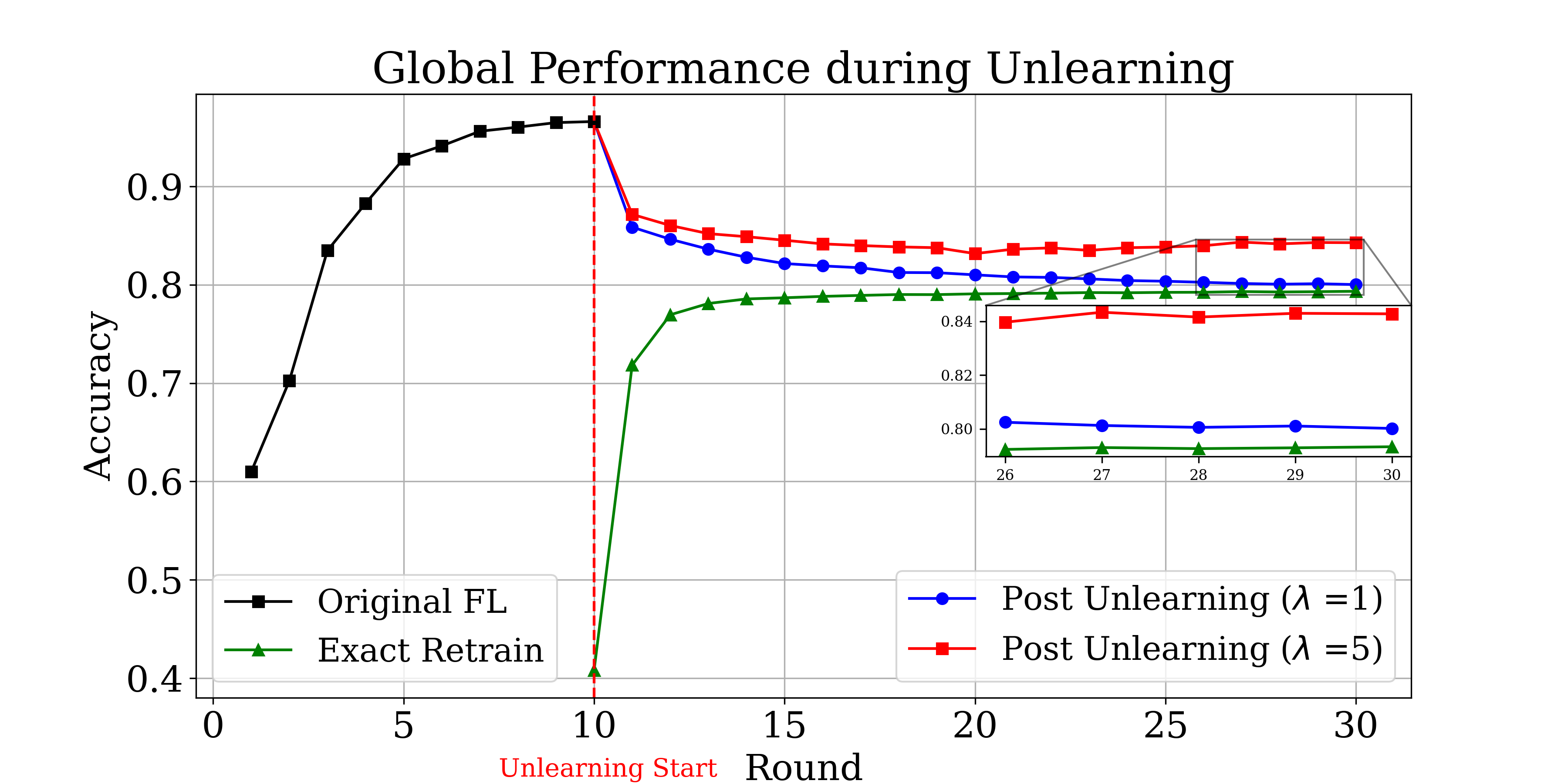
Figure 4: Unlearning Convergence and Handling Stability: Increasing stability penalty $\lambda$ enhances global performance of FU.

7 Experiments

7.1 Experiment Settings

In our experiment, we utilize the MNIST dataset (LeCun et al., ) non-IID distributed across ten clients, each holding four distinct classes (the data distribution is detailed in Appendix G). We employ LeNet-5 architecture (LeCun et al., 1998), a classic non-convex neural network model, to evaluate FU’s consequences. To straightforwardly assess the FU evaluations metrics ($V,S,Q$), we focus on accuracy, e.g., $V=-Acc_{-\mathcal{J}}(\boldsymbol{{w}}^{u})+Acc_{-\mathcal{J}}(\boldsymbol{w}^{r*})$ (in percentage). A smaller value of these metrics indicates better effectiveness, stability, or fairness achieved by our FU mechanism. We further conduct additional experiments focusing on data heterogeneity and employ different datasets, as detailed in Appendix G. The overall experimental evaluation confirms our FU mechanisms in balancing the trade-offs, aligning with the theoretical insights in Section 5.

7.2 FU for Balancing Stability

We examine the stability penalty $\lambda$ in our FU mechanism in Section 6.1 and unlearning clients $[3,4,8]$ starts at round $10$ where the FL model has converged.

Unlearning Convergence and Handling Stability. The heterogeneity between remaining and unlearned clients leads to instability after unlearning (discussed in Lemma 5.8), as indicated by the reduced global performance after retraining in Figure 4. Additionally, Figure 4 showcases the convergence of our FU mechanism with different stability penalties $\lambda$ in the context of global performance. Specifically, with a stability penalty $\lambda=1$, unlearning shows better stability than exact retraining. Increasing $\lambda$ to 5 further improves the stability of FU.

Balancing Verification and Stability: As shown in Figure 5, increasing $\lambda$ lowers $V+S$, improving the balance between verification and stability in FU. Although a higher $\lambda$ reduces FU effectiveness (increasing $V$), our FU mechanism allows a better trade-off within a certain tolerance level for $V$. Additionally, it demonstrates time efficiency compared to retraining in Table 1, making it practical in real-world FU scenarios.

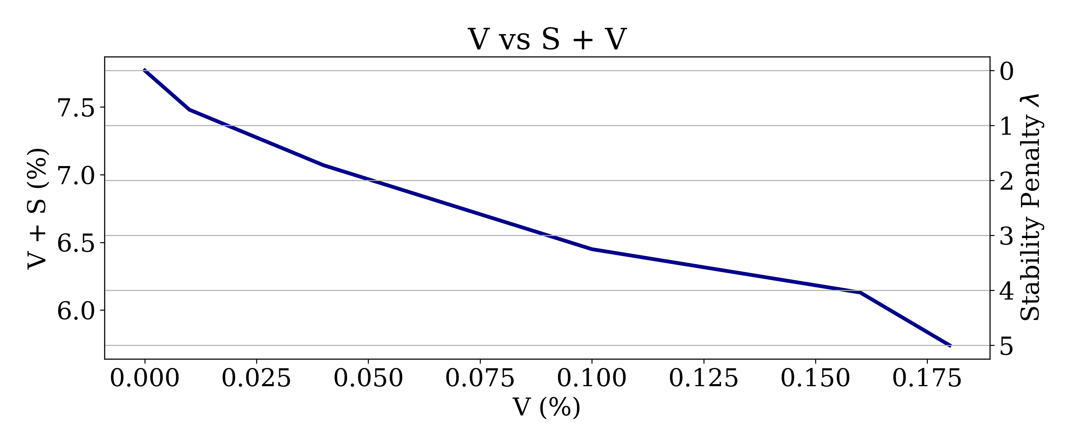
Figure 5: Trade-offs with Stability Penalty $\lambda$: Increasing $\lambda$ improves the balance between FU verification and stability, reflected by reduced $V+S$.

Table 1: Unlearning Efficiency Compared to Retraining.
(Computing Resources: 2 Intel Xeon Gold 5217 CPUs, 384GB RAM, and 8 Nvidia GeForce RTX-2080Ti GPUs)

	Faster than Retrain ($\times$)
$\lambda=1$	1.425$\pm$0.057
$\lambda=3$	2.103$\pm$0.149
$\lambda=5$	3.211 $\pm$0.315

7.3 FU for Balancing Fairness

Considering a higher data heterogeneity between unlearned and remaining clients, unlearning clients [2, 10] leads to a maximum performance drop of 1.5% ($\epsilon=1.5$) for client 6. We employ the FU mechanism in Section 6.2 with a fairness constraint $\epsilon=1$ and $\Lambda=1.3$ ensuring no client’s performance deviates beyond $\epsilon$. This setting yields the FU verification metric $V=0.57$. We further tighten $\epsilon$ to $1$, and observe $V$ reduces to $0.11$. This enhancing FU effectiveness and fairness is consistent with insights on data heterogeneity in Lemma 6.8 and Theorem 5.11.

8 Conclusion

In this study, we investigated the trade-offs in FU under data heterogeneity, focusing on balancing unlearning verification with global stability and local fairness. We proposed a novel FU mechanism grounded in a comprehensive theoretical framework with optimization strategies and penalty controls. Our findings highlight the impacts of data heterogeneity in FU, paving the way for future research to explore adaptive FU mechanisms.

Appendix A Proof of Lemma 5.6

Proof.

Given the FU verification metric $V(\boldsymbol{{w}}^{u})=\mathbb{E}\left[F_{-\mathcal{J}}(\boldsymbol{{w}}^{u})\right]-F_{-\mathcal{J}}(\boldsymbol{w}^{r*})$, we analyze the metric using iterative updates in the FU process.

For each iteration $t+1$:

$$F_{-\mathcal{J}}(\boldsymbol{w}^{t+1})-F_{-\mathcal{J}}(\boldsymbol{w}^{t}) \geq\left\langle\nabla F_{-\mathcal{J}}(\boldsymbol{w}^{t}),\boldsymbol{w}^{t+1}-\boldsymbol{w}^{t}\right\rangle+\frac{\mu}{2}\|\boldsymbol{w}^{t+1}-\boldsymbol{w}^{t}\|^{2}$$

$$=\left\langle-\eta\boldsymbol{g}_{\mathcal{S}}^{t},\nabla F_{-\mathcal{J}}(\boldsymbol{w}^{t})\right\rangle+\frac{\mu\eta^{2}}{2}\|\boldsymbol{g}_{\mathcal{S}}^{t}\|^{2}$$

where $\boldsymbol{g}_{\mathcal{S}}^{t}=\sum_{i\in\mathcal{S}}\alpha_{i}\boldsymbol{g}_{i}^{t}$, and $\alpha_{i}$ is the aggregation weight of client $i$.

Taking expectations on both sides, we derive:

$$\mathbb{E}\left[F_{-\mathcal{J}}(\boldsymbol{w}^{t+1})\right]-F_{-\mathcal{J}}(\boldsymbol{w}^{t})\geq\frac{\eta}{2}\underbrace{\left\|\boldsymbol{G}_{\mathcal{S}}^{t}-\nabla F_{-\mathcal{J}}(\boldsymbol{w}^{t})\right\|^{2}}_{A_{1}}\underbrace{-\frac{\eta}{2}\|\nabla F_{-\mathcal{J}}(\boldsymbol{w}^{t})\|^{2}-\frac{\eta}{2}\left\|\boldsymbol{G}_{\mathcal{S}}^{t}\right\|^{2}+\frac{\mu\eta^{2}}{2}\mathbb{E}\|\boldsymbol{g}_{\mathcal{S}}^{t}\|^{2}}_{A_{2}}$$ (11)

where $\boldsymbol{G}_{\mathcal{S}}^{t}=\sum_{i\in\mathcal{S}}\alpha_{i}\boldsymbol{G}_{i}^{t}$, with $\boldsymbol{G}_{i}^{t}=\mathbb{E}\left[\boldsymbol{g}_{i}^{t}\right]$ representing the gradient for client $i$ at iteration $t$, while $\boldsymbol{g}_{i}^{t}$ denotes the stochastic gradient.

Firstly, for $A_{1}$:

$$\left\|\boldsymbol{G}_{\mathcal{S}}^{t}-\nabla F_{-\mathcal{J}}(\boldsymbol{w^{t}})\right\|^{2}\leq\mathbb{E}_{i}\left\|\boldsymbol{G}_{i}^{t}-\nabla F_{-\mathcal{J}}(\boldsymbol{w^{t}})\right\|^{2}\underset{\lx@cref{creftype~refnum}{ass:data-heterogeneity}}{\leq}\zeta_{\mathcal{S}}^{2}+\beta_{\mathcal{S}}^{2}\|\nabla F_{-\mathcal{J}}(\boldsymbol{w^{t}})\|^{2}$$ (12)

Let $\left\|\boldsymbol{G}_{\mathcal{S}}^{t}-\nabla F_{-\mathcal{J}}(\boldsymbol{w^{t}})\right\|^{2}=\zeta_{t}^{2}+\beta_{\mathcal{S}}^{2}\|\nabla F_{-\mathcal{J}}(\boldsymbol{w^{t}})\|$, where $\zeta_{t}^{2}$ is specific for each round $t$ ($\zeta_{t}^{2}\leq\zeta_{\mathcal{S}}^{2}$).

Applying the triangle inequality, we derive the following relation for $A_{1}$: $\|\boldsymbol{G}_{\mathcal{S}}^{t}\|^{2}\geq\zeta_{t}^{2}+(\beta_{\mathcal{S}}^{2}-1)\|\nabla F_{-\mathcal{J}}(\boldsymbol{w^{t}})\|^{2}$.

Then, for $A_{2}$, we expand it as follows:

$$A_{2}=\frac{\mu\eta^{2}}{2}\underbrace{\mathbb{E}\left\|\boldsymbol{G}_{\mathcal{S}}^{t}-\boldsymbol{g}_{\mathcal{S}}^{t}\right\|^{2}}_{=\sigma_{t}^{2}\leq\sigma^{2}(\lx@cref{creftype~refnum}{ass:unbiased_gradient})}+\frac{\eta}{2}\left(\eta\mu-1\right)\left\|\boldsymbol{G}_{\mathcal{S}}^{t}\right\|^{2}-\frac{\eta}{2}\left\|\nabla F_{-\mathcal{J}}(\boldsymbol{w}^{t})\right\|^{2}$$ (13)

Now, by Equation 12 and Equation 13, taking expectation on both sides of Appendix A:

$$\mathbb{E}\left[F_{-\mathcal{J}}(\boldsymbol{w}^{t+1})\right]-F_{-\mathcal{J}}(\boldsymbol{w}^{t}) \geq\frac{\eta}{2}\underbrace{\left(\zeta_{t}^{2}+\beta_{\mathcal{S}}^{2}\|\nabla F_{-\mathcal{J}}(\boldsymbol{w}^{t})\|^{2}\right)}_{=A_{1}}$$ (14)

$$\quad+\underbrace{\frac{\mu\eta^{2}}{2}\sigma_{t}^{2}+\frac{\eta}{2}\left(\eta\mu\beta_{\mathcal{S}}^{2}-\eta\mu-\beta_{\mathcal{S}}^{2}\right)\|\nabla F_{-\mathcal{J}}(\boldsymbol{w}^{t})\|^{2}+\frac{\eta}{2}\left(\eta\mu-1\right)\zeta_{t}^{2}}_{\leq A_{2}}$$

$$=\frac{\mu\eta^{2}}{2}\left(\beta_{\mathcal{S}}^{2}-1\right)\|\nabla F_{-\mathcal{J}}(\boldsymbol{w}^{t})\|^{2}+\frac{\eta^{2}\mu}{2}\left(\sigma_{t}^{2}+\zeta_{t}^{2}\right)$$

$$\geq\underbrace{\frac{\mu\eta^{2}}{2}M\left(\beta_{\mathcal{S}}^{2}-1\right)}_{B_{1}}\left(F_{-\mathcal{J}}(\boldsymbol{w}^{t})-F_{-\mathcal{J}}(\boldsymbol{w}^{r*})\right)+\frac{\eta^{2}\mu}{2}\left(\sigma_{t}^{2}+\zeta_{t}^{2}\right),$$ (15)

where $M=2\mu$ if $\beta_{\mathcal{S}}\geq 1$, else $M=2L$.

Let $\bar{\sigma^{2}}=\frac{1}{T}\sum_{t=1}^{T}\sigma_{t}^{2}$ and $\bar{\zeta^{2}}=\frac{1}{T}\sum_{t=1}^{T}\zeta_{t}^{2}$. Thus, by iterative updates, we have:

$$\mathbb{E}\left[F_{-\mathcal{J}}(\boldsymbol{w}^{T})\right]-F_{-\mathcal{J}}(\boldsymbol{w}^{r*})\geq\left(B_{1}+1\right)^{T}\left(F_{-\mathcal{J}}(\boldsymbol{\boldsymbol{w}}^{o})-F_{-\mathcal{J}}(\boldsymbol{w}^{r*})\right)+\frac{\eta^{2}\mu}{2}(\bar{\sigma^{2}}+\bar{\zeta^{2}})\sum_{r=1}^{T}\left(B_{1}+1\right)^{T-r}$$ (16)

Taking $\eta^{2}=\frac{2}{\mu MT^{2}}$, we have $B_{1}=\frac{2(\beta_{\mathcal{S}}^{2}-1)}{T^{2}}$.

Now, considering two cases for $B_{1}$:

Case 1: If $B_{1}\leq-1$ (since $T^{2}\geq 1$, Case 1 only holds when $T=1$ and $\beta_{\mathcal{S}}^{2}\leq\frac{1}{2}$), we get:

$$\mathbb{E}\left[F_{-\mathcal{J}}(\boldsymbol{w}^{T})\right]-F_{-\mathcal{J}}(\boldsymbol{w}^{r*})\geq\left(1+2(\beta_{\mathcal{S}}^{2}-1)\right)\left(F_{-\mathcal{J}}(\boldsymbol{\boldsymbol{w}}^{o})-F_{-\mathcal{J}}(\boldsymbol{w}^{r*})\right)+\frac{1}{M}\left(\bar{\sigma^{2}}+\bar{\zeta^{2}}\right),$$ (17)

Case 2: If $B_{1}\geq-1$, then $(B_{1}+1)^{T}\geq 1+TB_{1}$, which leads to the inequality:

$$\mathbb{E}\left[F_{-\mathcal{J}}(\boldsymbol{w}^{T})\right]-F_{-\mathcal{J}}(\boldsymbol{w}^{r*})\geq\left(1+2\frac{\beta_{\mathcal{S}}^{2}-1}{T}\right)\left(F_{-\mathcal{J}}(\boldsymbol{\boldsymbol{w}}^{o})-F_{-\mathcal{J}}(\boldsymbol{w}^{r*})\right)+\rho\left(\bar{\sigma^{2}}+\bar{\zeta^{2}}\right),$$ (18)

where $\rho=\frac{\eta^{2}\mu}{2B_{1}}\left(\left(B_{1}+1\right)^{T}-1\right)\geq 0$ for $\forall B_{1}\geq-1$. Therefore, we can derive $\rho\geq\frac{\eta^{2}\mu T}{2}=\frac{1}{MT}$

Combining two cases and ${M}\leq{2L}$, we conclude

$$~{}\mathbb{E}\left[F_{-\mathcal{J}}(\boldsymbol{w}^{T})\right]-F_{-\mathcal{J}}(\boldsymbol{w}^{r*}) \geq\left(1+2\frac{\beta_{\mathcal{S}}^{2}-1}{T}\right)\left(F_{-\mathcal{J}}(\boldsymbol{\boldsymbol{w}}^{o})-F_{-\mathcal{J}}(\boldsymbol{w}^{r*})\right)+\frac{1}{2LT}\left(\bar{\sigma^{2}}+\bar{\zeta^{2}}\right),$$ (19)

∎

Appendix B Proof of Lemma 5.8

Proof.

Given the stability metric $S(\boldsymbol{{w}}^{u})$, we express it as

$$S(\boldsymbol{{w}}^{u})=\mathbb{E}\left[F(\boldsymbol{{w}}^{u})\right]-F(\boldsymbol{w}^{*})=A_{1}+A_{2},$$ (20)

where $A_{1}=\mathbb{E}\left[F(\boldsymbol{{w}}^{u})\right]-F(\boldsymbol{\boldsymbol{w}}^{o})$ and $A_{2}=F(\boldsymbol{\boldsymbol{w}}^{o})-F(\boldsymbol{w}^{*})=\delta$. $A_{2}$ represents the empirical risk minimization (ERM) gap.

Firstly, to bound $A_{1}$, we utilize the convexity of $F$: $A_{1}\geq\left\langle\nabla F(\boldsymbol{\boldsymbol{w}}^{o}),\mathbb{E}\left[\boldsymbol{{w}}^{u}-\boldsymbol{\boldsymbol{w}}^{o}\right]\right\rangle+\frac{\mu}{2}\mathbb{E}\left[\|\boldsymbol{{w}}^{u}-\boldsymbol{\boldsymbol{w}}^{o}\|^{2}\right]$.

With $\boldsymbol{{w}}^{u}-\boldsymbol{\boldsymbol{w}}^{o}=-\eta\sum_{r=1}^{T}\mathbf{g}_{r}^{(\mathcal{S})}$, and $\mathbf{g}_{r}^{(\mathcal{S})}$ being the aggregated stochastic gradient from the subset of remaining clients $\mathcal{S}\subseteq\mathcal{N}\setminus\mathcal{J}$, let $\bar{\mathbf{g}}^{(\mathcal{S})}=\frac{1}{T}\sum_{r=1}^{T}\mathbf{g}_{r}^{(\mathcal{S})}$, we have $\boldsymbol{{w}}^{u}-\boldsymbol{\boldsymbol{w}}^{o}=-\eta T\bar{\mathbf{g}}^{(\mathcal{S})}$.

Considering FL with remaining clients, the global objective is $F_{-\mathcal{J}}=\sum_{i\notin\mathcal{J}}p_{i}^{\prime}f_{i}$, where $p_{i}^{\prime}=\frac{p_{i}}{1-P_{\mathcal{J}}}$.

For FL with unlearned clients, the global objective is $F_{\mathcal{J}}=\sum_{j\in\mathcal{J}}p_{j}^{\prime}f_{j}$, where $p_{j}^{\prime}=\frac{p_{j}}{P_{\mathcal{J}}}$. Then, $\nabla F(\boldsymbol{\cdot})=(1-P_{\mathcal{J}})\nabla F_{-\mathcal{J}}(\cdot)+P_{\mathcal{J}}\nabla F_{\mathcal{J}}(\cdot)$.

Expanding $A_{1}$, we get:

$$=\frac{(1-P_{\mathcal{J}})\eta T}{2}\mathbb{E}\left[\|\nabla F_{-\mathcal{J}}(\boldsymbol{\boldsymbol{w}}^{o})-\bar{\mathbf{g}}^{(\mathcal{S})}\|^{2}\right]+\frac{P_{\mathcal{J}}\eta T}{2}\mathbb{E}\left[\|\nabla F_{\mathcal{J}}(\boldsymbol{\boldsymbol{w}}^{o})-\bar{\mathbf{g}}^{(\mathcal{S})}\|^{2}\right]$$

$$\quad-\frac{(1-P_{\mathcal{J}})\eta T}{2}\|\nabla F_{-\mathcal{J}}(\boldsymbol{\boldsymbol{w}}^{o})\|^{2}-\frac{P_{\mathcal{J}}\eta T}{2}\|\nabla F_{\mathcal{J}}(\boldsymbol{\boldsymbol{w}}^{o})\|^{2}$$

$$\quad-\frac{\eta T}{2}\mathbb{E}\left[\|\bar{\mathbf{g}}^{(\mathcal{S})}\|^{2}\right]+\frac{\mu\eta^{2}T^{2}}{2}\mathbb{E}\left[\|\bar{\mathbf{g}}^{(\mathcal{S})}\|^{2}\right],$$ (21)

Under 5.5 where $1-P_{\mathcal{J}}\geq P_{\mathcal{J}}$, and 6.1 where gradient norm is bounded ($\|\nabla F\|^{2}\leq G^{2}$), taking $T\geq\frac{\mu}{\eta^{2}}$, we can derive the lower bound for $A_{1}$:

$$A_{1} \geq\frac{P_{\mathcal{J}}\eta T}{2}\|\nabla F_{-\mathcal{J}}(\boldsymbol{\boldsymbol{w}}^{o})-\nabla F_{\mathcal{J}}(\boldsymbol{\boldsymbol{w}}^{o})\|^{2}+\frac{\eta^{2}T^{2}-\mu T}{2}(\|\bar{\mathbf{G}}^{(\mathcal{S})}\|^{2}+\sigma^{2})+\frac{\eta T}{2}G^{2}$$

$$\underset{T\geq\frac{\mu}{\eta^{2}}}{\geq}\frac{P_{\mathcal{J}}\eta T}{2}\|\nabla F_{-\mathcal{J}}(\boldsymbol{\boldsymbol{w}}^{o})-\nabla F_{\mathcal{J}}(\boldsymbol{\boldsymbol{w}}^{o})\|^{2}$$ (22)

Therefore, we obtain the lower bound for $S$ in FU:

$$~{}S(\boldsymbol{{w}}^{u})\geq\frac{P_{\mathcal{J}}\eta T}{2}\|\nabla F_{-\mathcal{J}}(\boldsymbol{\boldsymbol{w}}^{o})-\nabla F_{\mathcal{J}}(\boldsymbol{\boldsymbol{w}}^{o})\|^{2}+\delta$$ (23)

∎

Appendix C Proof of Theorem 5.10

Proof.

By setting $\eta=\frac{1}{T}\sqrt{\frac{2}{\mu M}}$, we ensure the inequality in Equation 19 is satisfied. Given the fact that $\frac{1}{M}\leq\frac{1}{2\mu}$, it follows that $\eta\leq\frac{1}{\mu T}$. Therefore, the inequality in Equation 23 also holds, completing the proof. ∎

Appendix D Proof of Theorem 5.11

Proof.

Starting with the local fairness metric $Q(\boldsymbol{{w}}^{u})$, we have:

$$Q(\boldsymbol{{w}}^{u}) =\sum_{i\notin\mathcal{J}}p_{i}^{\prime}\left|\Delta f_{i}-\sum_{i\notin\mathcal{J}}p_{i}^{\prime}\Delta f_{i}\right|$$

$$=\sum_{i\notin\mathcal{J}}p_{i}^{\prime}\left|\Delta f_{i}-V+F_{\mathcal{J}}(\boldsymbol{w}^{*})-F_{-\mathcal{J}}^{*}\right|$$

$$\geq\sum_{i\notin\mathcal{J}}p_{i}^{\prime}\left|\Delta f_{i}\right|-V-\left(F_{\mathcal{J}}(\boldsymbol{w}^{*})-F_{-\mathcal{J}}^{*}\right)$$

$$\geq-2V+F_{-\mathcal{J}}^{*}-\sum_{i\notin\mathcal{J}}p_{i}^{\prime}f_{i}(\boldsymbol{w_{i}}^{*}).$$ (24)

The last inequality arises from:

$$\sum_{i\notin\mathcal{J}}p_{i}^{\prime}\left|\Delta f_{i}\right| =\sum_{i\notin\mathcal{J}}p_{i}^{\prime}\left|\mathbb{E}\left[f_{i}(\boldsymbol{{w}}^{u})\right]-f_{i}(\boldsymbol{w}^{*})\right|$$

$$=\sum_{i\notin\mathcal{J}}p_{i}^{\prime}\left|\left(f_{i}(\boldsymbol{w}^{*})-f_{i}(\boldsymbol{w_{i}}^{*})\right)-\left(\mathbb{E}\left[f_{i}(\boldsymbol{{w}}^{u})\right]-f_{i}(\boldsymbol{w_{i}}^{*})\right)\right|$$

$$\geq\sum_{i\notin\mathcal{J}}p_{i}^{\prime}\left(f_{i}(\boldsymbol{w}^{*})-f_{i}(\boldsymbol{w_{i}}^{*})\right)-\sum_{i\notin\mathcal{J}}p_{i}^{\prime}\left(\mathbb{E}\left[f_{i}(\boldsymbol{{w}}^{u})\right]-f_{i}(\boldsymbol{w_{i}}^{*})\right)$$

$$\underset{(1)}{\geq}F_{-\mathcal{J}}(\boldsymbol{w}^{*})-\sum_{i\notin\mathcal{J}}p_{i}^{\prime}f_{i}(\boldsymbol{w_{i}}^{*})-\left(\mathbb{E}\left[F_{-\mathcal{J}}(\boldsymbol{{w}}^{u})\right]-F_{\mathcal{J}}^{*}\right)$$

$$=F_{-\mathcal{J}}(\boldsymbol{w}^{*})-\sum_{i\notin\mathcal{J}}p_{i}^{\prime}f_{i}(\boldsymbol{w_{i}}^{*})-V.$$ (25)

The inequality (1) is justified because $\sum_{i\notin\mathcal{J}}p_{i}^{\prime}f_{i}(\boldsymbol{w_{i}}^{*})\leq F_{-\mathcal{J}}^{*}$, as $\min_{\boldsymbol{w}}F_{-\mathcal{J}}(\boldsymbol{w})\geq\sum_{i\notin\mathcal{J}}p_{i}^{\prime}\min_{\boldsymbol{w}}f_{i}(\boldsymbol{w})$.

Therefore,

$$Q(\boldsymbol{{w}}^{u})+2V(\boldsymbol{{w}}^{u})\leq F_{-\mathcal{J}}^{*}-\sum_{i\notin\mathcal{J}}p_{i}^{\prime}f_{i}(\boldsymbol{w_{i}}^{*}).$$

∎

Appendix E Balancing Stability Unlearning Algorithm Analysis

E.1 Proof for Theorem 6.4

Lemma E.1.

Lemma 1 of (Li et al., 2020b) Let 5.1 holds and $\eta_{l}\leq\frac{1}{4L}$, the remaining clients’ contribution to unlearning for every round $t$ gives:

$${\mathbb{E}\left[\left\|{\boldsymbol{\bar{w}}}^{(t,E)}-\boldsymbol{w}^{r*}\right\|^{2}\right]}\leq(1-\eta_{l}\mu)\mathbb{E}\left[\left\|{\boldsymbol{\bar{w}}}^{(t,0)}-\boldsymbol{w}^{r*}\right\|^{2}\right]+\eta_{l}^{2}C$$ (26)

where $C=\sigma^{2}+6L\Gamma+8(E-1)^{2}\left(\zeta_{\mathcal{S}}^{2}+(\beta_{\mathcal{S}}^{2}+1)G^{2}\right)$, $\Gamma=F_{-\mathcal{J}}^{*}-\sum_{i\in\mathcal{S}}\alpha_{i}F_{i}^{*}$ and $\boldsymbol{w}^{r*}=argmin_{\boldsymbol{w}}F_{-\mathcal{J}}(\boldsymbol{w})$ is the optimal unlearned model.

Proof.

Suppose the FU process involves a total of $T$ unlearning rounds, and within each round $t$, each participating client $i$ engages in $E$ local iterations. During local iterations, client $i$’s model at iteration $\tau$ ($\tau\leq E$) of round $t$ is denoted as $\boldsymbol{w}^{(t,\tau)}_{i}$. At the end of round $t$, the server aggregates to obtain the global model ${\boldsymbol{\bar{w}}}^{(t,E)}$ and updates the global model by gradient correction as ${\boldsymbol{\bar{w}}}^{(t+1,0)}={\boldsymbol{\bar{w}}}^{(t,E)}-\eta_{g}\boldsymbol{g}_{c}^{t}$.

Then, we can express ${\boldsymbol{\bar{w}}}^{(t+1,0)}={\boldsymbol{\bar{w}}}^{(t,0)}-\eta_{l}\boldsymbol{g}_{\mathcal{S}}^{t}-\eta_{g}\boldsymbol{g}_{c}^{t}$, and we have:

$$\mathbb{E}\left[\left\|{\boldsymbol{\bar{w}}}^{(t+1,0)}-\boldsymbol{w}^{r*}\right\|^{2}\right] =\mathbb{E}\left[\left\|{\boldsymbol{\bar{w}}}^{(t,0)}-\eta_{l}\boldsymbol{g}_{\mathcal{S}}^{t}-\eta_{g}\boldsymbol{g}_{c}^{t}-\boldsymbol{w}^{r*}\right\|^{2}\right]$$

$$=\underbrace{\mathbb{E}\left[\left\|{\boldsymbol{\bar{w}}}^{(t,0)}-\eta_{l}\boldsymbol{g}_{\mathcal{S}}^{t}-\boldsymbol{w}^{r*}\right\|^{2}\right]}_{R^{t}}+\underbrace{\eta_{g}^{2}\mathbb{E}\left[\left\|\boldsymbol{g}_{c}^{t}\right\|^{2}\right]-2\eta_{g}\mathbb{E}\left[\left\langle{\boldsymbol{\bar{w}}}^{(t,0)}-\boldsymbol{w}^{r*},\boldsymbol{g}_{c}^{t}\right\rangle\right]}_{\Phi^{t}}$$ (27)

where $R^{t}$ can be bounded by Lemma E.1.

Then, we will bound the second term $\Phi^{t}$ in Section E.1. By Cauchy-Schwarz inequality and AM-GM inequality, we have $-2\left\langle\boldsymbol{g}_{c}^{t},{\boldsymbol{\bar{w}}}^{(t,0)}-\boldsymbol{w}^{r*}\right\rangle\leq{\eta_{g}}\left\|\boldsymbol{g}_{c}^{t}\right\|^{2}+\frac{1}{\eta_{g}}\left\|{\boldsymbol{\bar{w}}}^{(t,0)}-\boldsymbol{w}^{r*}\right\|^{2}$

Thus,

$$\Phi^{t} \leq\mathbb{E}\left[\left\|{\boldsymbol{\bar{w}}}^{(t,0)}-\boldsymbol{w}^{r*}\right\|^{2}\right]+2\eta_{g}^{2}\mathbb{E}\left[\left\|\boldsymbol{g}_{c}^{t}\right\|^{2}\right]$$

$$\underset{\text{\lx@cref{creftype~refnum}{lemma:bounded_gradient_correction}}}{\leq}\mathbb{E}\left[\left\|{\boldsymbol{\bar{w}}}^{(t,0)}-\boldsymbol{w}^{r*}\right\|^{2}\right]+2\eta_{g}^{2}\zeta^{\prime 2}\phi+2\eta_{g}^{2}(\beta^{\prime 2}+1)\phi\left\|\nabla F_{-\mathcal{J}}({\boldsymbol{\bar{w}}}^{t,0})\right\|^{2}$$

$$\underset{\text{\lx@cref{creftype~refnum}{ass:bounded-gradient}}}{\leq}\mathbb{E}\left[\left\|{\boldsymbol{\bar{w}}}^{(t,0)}-\boldsymbol{w}^{r*}\right\|^{2}\right]+2\eta_{g}^{2}\zeta^{\prime 2}\phi+2\eta_{g}^{2}\phi\Omega G^{2}$$ (28)

where $\Omega=(\beta^{\prime 2}+1)$, $\beta^{\prime 2}$ indicates the data heterogeneity between remaining and unlearned clients.

Under Lemma E.1, taking Section E.1 into Section E.1 and letting $\Delta_{t}=\mathbb{E}\left[\left\|{\boldsymbol{\bar{w}}}^{(t,0)}-\boldsymbol{w}^{r*}\right\|^{2}\right]$, we have:

$$\Delta_{t+1}\leq\left(2-\eta_{l}\mu\right)\Delta_{t}+\eta_{l}^{2}B$$ (29)

where $B=\sigma^{2}+6L\Gamma+8\left(\zeta_{\mathcal{S}}^{2}+(\beta_{\mathcal{S}}^{2}+1)G^{2}\right)(E-1)^{2}+2\phi(\frac{\eta_{g}}{\eta_{l}})^{2}(\Omega\phi G^{2}+\zeta^{\prime 2})$

Next, we will prove $\Delta_{t}\leq\frac{v}{\gamma+t}$ where $v=\max\left\{\frac{\beta^{2}B}{\beta\mu-4},(\gamma+1)\Delta_{1}\right\}$. For a diminishing stepsize, $\eta_{l}=\frac{\beta}{2(t+\gamma)}$ for some $\beta>\frac{1}{\mu}$ and $\gamma>0$ such that $\eta_{l}\leq\frac{1}{4L}$. We prove $\Delta_{t}\leq\frac{v}{\gamma+t}$ by induction.

Firstly, the definition of $v$ ensures that it holds for $t=1$. Assume the conclusion holds for some $t$, it follows that

$$\Delta_{t+1} \leq\left(2-\eta_{t}\mu\right)\Delta_{t}+\eta_{t}^{2}B$$

$$\leq\left(2-\frac{\beta\mu}{2(t+\gamma)}\right)\frac{v}{2(t+\gamma)}+\frac{\beta^{2}B}{4(t+\gamma)^{2}}$$

$$=\frac{4(t+\gamma)-4}{4(t+\gamma)^{2}}v+\left[\frac{\beta^{2}B}{4(t+\gamma)^{2}}-\frac{\beta\mu-4}{4(t+\gamma)^{2}}v\right]$$

$$\leq\frac{v}{t+\gamma+1}$$

By the $L$-smoothness of $H(\cdot)$,

$$\mathbb{E}\left[H\left({\boldsymbol{\bar{w}}}^{(t,0)}\right)\right] -H^{*}$$

$$=\mathbb{E}\left[H\left({\boldsymbol{\bar{w}}}^{(t,0)}\right)\right]-H(\boldsymbol{w}^{r*})+H(\boldsymbol{w}^{r*})-H^{*}$$

$$\leq\frac{L}{2}\Delta_{t}+\frac{L}{2}\left\|\boldsymbol{w}^{r*}-\boldsymbol{w}^{*}\right\|^{2}$$

$$\leq\frac{L}{2}\left(\frac{v}{\gamma+t}+\left\|\boldsymbol{w}^{r*}-\boldsymbol{w}^{*}\right\|^{2}\right)$$

∎

E.2 Proof for Theorem 6.7

Additional Lemmas

Lemma E.2.

Under 6.2 and 6.5, the expected norm of the gradient correction term at round $t$ is bounded as follows:

$$\mathbb{E}\left[\left\|\boldsymbol{g_{c}}({\boldsymbol{\bar{w}}}^{(t,E)})\right\|^{2}\right]\leq\phi\left(\zeta^{\prime 2}+(\beta^{\prime 2}+1)\epsilon\left\|\nabla F_{-\mathcal{J}}({\boldsymbol{\bar{w}}}^{t,0})\right\|^{2}\right)$$

, where $\phi=\lambda^{2}P_{\mathcal{J}}^{2}(1+\cos^{2}\theta)$. $\cos^{2}\theta$ represents $\cos^{2}\theta$ represents the similarity between the objectives of the remaining and unlearned clients.

Lemma E.3 (Per Round Unlearning).

For each iteration $t$ in the unlearning process:

$$\mathbb{E}\left[F_{-\mathcal{J}}(\boldsymbol{w}^{t+1})-F_{-\mathcal{J}}(\boldsymbol{w}^{t})\right]$$

$$\leq\underbrace{\mathbb{E}\left[\left\langle-\eta_{l}\boldsymbol{g}_{\mathcal{S}}^{t},\nabla F_{-\mathcal{J}}(\boldsymbol{w}^{t})\right\rangle\right]+\frac{L\eta_{l}^{2}}{2}\mathbb{E}\left[\left\|\boldsymbol{g}_{\mathcal{S}}^{t}\right\|^{2}\right]}_{A_{1}:\text{remaining clients training}}$$

$$\quad+\underbrace{\mathbb{E}\left[\left\langle-\eta_{g}\boldsymbol{g_{c}}^{t},\nabla F_{-\mathcal{J}}(\boldsymbol{w}^{t})\right\rangle\right]+\frac{L\eta_{g}^{2}}{2}\mathbb{E}\left[\left\|\boldsymbol{g_{c}}^{t}\right\|^{2}\right]}_{A_{2}:\text{global correction}}$$

Proof.

Based on Lemma E.3, we can decomposed the convergence of unlearning verficiation $V=\mathbb{E}[F_{-\mathcal{J}}(\boldsymbol{w}^{t+1})-F_{-\mathcal{J}}(\boldsymbol{w}^{t})]$ into two primary components $A_{1}$ and $A_{2}$:

$$\frac{1}{2}\mathbb{E}\left[F_{-\mathcal{J}}(\boldsymbol{w}^{t+1})-F_{-\mathcal{J}}(\boldsymbol{w}^{t})\right]\leq A_{1},\qquad\frac{1}{2}\mathbb{E}\left[F_{-\mathcal{J}}(\boldsymbol{w}^{t+1})-F_{-\mathcal{J}}(\boldsymbol{w}^{t})\right]\leq A_{2}$$

These components $A_{1}$ represent the impact of training with the remaining clients, and $A_{2}$ represents the global correction.

Derivation for component $A_{1}$:

For $A_{1}$, it is related to unlearning with the remaining clients. By iterative derivation, we have

$$\frac{1}{2}\mathbb{E}\left[F_{-\mathcal{J}}(\boldsymbol{w}^{t+1})\right]-F_{-\mathcal{J}}(\boldsymbol{w}^{t}) \leq A_{1}=\frac{\eta_{l}}{2}\mathbb{E}\left[\left\|\boldsymbol{g}_{\mathcal{S}}^{t}-\nabla F_{-\mathcal{J}}(\boldsymbol{w}^{t})\right\|^{2}\right]-\frac{\eta_{l}}{2}{\left\|\boldsymbol{G}_{\mathcal{S}}^{t}\right\|^{2}}-\frac{\eta_{l}}{2}\left\|\nabla F_{-\mathcal{J}}(\boldsymbol{w}^{t})\right\|^{2}+\frac{L\eta_{l}^{2}}{2}\left\|\boldsymbol{g}_{\mathcal{S}}^{t}\right\|^{2}$$

$$=\frac{\eta_{l}}{2}\mathbb{E}\left[\left\|\boldsymbol{g}_{\mathcal{S}}^{t}-\nabla F_{-\mathcal{J}}(\boldsymbol{w}^{t})\right\|^{2}\right]+\frac{L\eta_{l}^{2}}{2}\mathbb{E}\left[\left\|\boldsymbol{G}_{\mathcal{S}}^{t}-\boldsymbol{g}_{\mathcal{S}}^{t}\right\|^{2}\right]$$

$$\qquad+\frac{\eta_{l}}{2}(\eta_{l}L-1)\left\|\boldsymbol{G}_{\mathcal{S}}^{t}\right\|^{2}-\frac{\eta_{l}}{2}\left\|\nabla F_{-\mathcal{J}}(\boldsymbol{w}^{t})\right\|^{2}$$

$$\leq_{\text{(\lx@cref{creftype~refnum}{ass:data-heterogeneity} \& \lx@cref{creftype~refnum}{ass:unbiased_gradient})}}\frac{\eta_{l}}{2}\left(\zeta_{\mathcal{S}}^{2}+\beta_{\mathcal{S}}^{2}\left\|\nabla F_{-\mathcal{J}}(\boldsymbol{w}^{t})\right\|^{2}\right)+\frac{L\eta_{l}^{2}}{2}\sigma^{2}$$

$$\qquad+\frac{\eta_{l}}{2}(\eta_{l}L-1)(\beta_{\mathcal{S}}^{2}+1)\left\|\nabla F_{-\mathcal{J}}(\boldsymbol{w}^{t})\right\|^{2}+\frac{\eta_{l}}{2}(\eta_{l}L-1)\zeta_{\mathcal{S}}^{2}$$

Thus,

$$\mathbb{E}\left[F_{-\mathcal{J}}(\boldsymbol{w}^{t+1})\right]-F_{-\mathcal{J}}(\boldsymbol{w}^{t})\leq\left({\eta_{l}^{2}L}(\beta_{\mathcal{S}}^{2}+1)-\frac{\eta_{l}}{2}\right)\left\|\nabla F_{-\mathcal{J}}(\boldsymbol{w}^{t})\right\|^{2}+{\eta_{l}^{2}L}\left(\sigma^{2}+\zeta_{\mathcal{S}}^{2}\right)$$

Taking $\eta_{l}=\frac{1}{LT}$ and $T\geq 2\beta_{\mathcal{S}}^{2}+2$ , we have:

$$\mathbb{E}\left[F_{-\mathcal{J}}(\boldsymbol{w}^{T})\right]-F_{-\mathcal{J}}(\boldsymbol{w}^{r*}) \leq\underbrace{\left(1-\frac{1}{2LT}+\frac{\beta_{\mathcal{S}}^{2}+1}{LT^{2}}\right)^{T}\left(F_{-\mathcal{J}}(\boldsymbol{\boldsymbol{w}}^{o})-F_{-\mathcal{J}}(\boldsymbol{w}^{r*})\right)}_{D_{1}}$$

$$\qquad+\underbrace{2\frac{\sigma^{2}+\zeta_{\mathcal{S}}^{2}}{(T-2\beta_{\mathcal{S}}^{2}-2)}\left(1-\left(1-\frac{T-2\beta_{\mathcal{S}}^{2}-2}{2LT^{2}}\right)^{T}\right)}_{D_{2}}$$

Bounding $D_{2}$: We will employ the inequality $(1-a)^{T}\leq 1-aT$ for $a\leq 1$. Here, $a=\frac{T-2\beta_{\mathcal{S}}^{2}-2}{2LT^{2}}$. Then, we verify that $a\leq 1$ by considering $2LT^{2}-T+2\beta_{\mathcal{S}}^{2}+2\geq 0$.

If $L(\beta_{\mathcal{S}}^{2}+1)\geq\frac{1}{16}$, then, $a\leq 1$ holds for $T\geq 1$. If $L(\beta_{\mathcal{S}}^{2}+1)<\frac{1}{16}$, then, considering $T\geq\frac{1+\Delta}{4L}$, where $\Delta=\sqrt{1-16L(\beta_{\mathcal{S}}^{2}+1)}$, we have $a\leq 1$.

Considering $T\geq\frac{1+\Delta}{4L}$ and we obtain $\left(1-\frac{T-2\beta_{\mathcal{S}}^{2}-2}{2LT^{2}}\right)^{T}\geq 1-\frac{T-2\beta_{\mathcal{S}}^{2}-2}{2LT}$, and

$$\frac{1}{(T-2\beta_{\mathcal{S}}^{2}-2)}\left(1-\left(1-\frac{T-2\beta_{\mathcal{S}}^{2}-2}{2LT^{2}}\right)^{T}\right)\leq\frac{1}{2LT}$$ (31)

By taking $T\geq\max\{2\beta_{\mathcal{S}}^{2}+2,\frac{1+\Delta}{4L}\}$ with $\Delta=\sqrt{\max\{0,1-16L(\beta_{\mathcal{S}}^{2}+1)\}}$, and integrating the bounds derived in Equation 31 into Section E.2, we have:

$$\mathbb{E}\left[F_{-\mathcal{J}}(\boldsymbol{w}^{T})\right]-F_{-\mathcal{J}}(\boldsymbol{w}^{r*}) \leq\left(1-\frac{1}{2LT}+\frac{\beta_{\mathcal{S}}^{2}+1}{LT^{2}}\right)^{T}\left(F_{-\mathcal{J}}(\boldsymbol{\boldsymbol{w}}^{o})-F_{-\mathcal{J}}(\boldsymbol{w}^{r*})\right)$$

$$\qquad+\frac{\sigma^{2}+\zeta_{\mathcal{S}}^{2}}{LT}$$

$$=2\chi_{1}.$$ (32)

Here, $\chi_{1}$ is defined as

$$\frac{1}{2}\left(1-\frac{1}{2LT}+\frac{\beta_{\mathcal{S}}^{2}+1}{LT^{2}}\right)^{T}\left(F_{-\mathcal{J}}(\boldsymbol{\boldsymbol{w}}^{o})-F_{-\mathcal{J}}(\boldsymbol{w}^{r*})\right)+\frac{(\sigma^{2}+\zeta_{\mathcal{S}}^{2})}{2LT}$$

.

Derivation for component $A_{2}$:

By Lemma E.3:

$$\frac{1}{2}\mathbb{E}\left[F_{-\mathcal{J}}(\boldsymbol{w}^{t+1})-F_{-\mathcal{J}}(\boldsymbol{w}^{t})\right]\leq A_{2}=\frac{L\eta_{g}^{2}}{2}\mathbb{E}\left[\left\|\boldsymbol{g_{c}}({\boldsymbol{\bar{w}}}^{(t,E)})\right\|^{2}\right]-\eta_{g}\mathbb{E}\left[\left\langle\boldsymbol{g_{c}}({\boldsymbol{\bar{w}}}^{(t,E)}),\nabla F_{-\mathcal{J}}({\boldsymbol{\bar{w}}}^{(t,0)})\right\rangle\right]$$

$$\quad={\frac{1}{2}({L\eta_{g}^{2}}-\eta_{g})}\mathbb{E}\left[\left\|\boldsymbol{g_{c}}({\boldsymbol{\bar{w}}}^{(t,E)})\right\|^{2}\right]+\frac{\eta_{g}}{2}\mathbb{E}\left[\left\|\boldsymbol{g_{c}}({\boldsymbol{\bar{w}}}^{(t,E)})-\nabla F_{-\mathcal{J}}({\boldsymbol{\bar{w}}}^{(t,0)})\right\|^{2}\right]-\frac{\eta_{g}}{2}\left\|\nabla F_{-\mathcal{J}}({\boldsymbol{\bar{w}}}^{(t,0)})\right\|^{2}$$

$$\quad\leq_{(1)}\frac{1}{2}{L\eta_{g}^{2}}\zeta^{{}^{\prime\prime}2}+\frac{1}{2}\left({L\eta_{g}^{2}}(\beta^{\prime\prime 2}+1)-2\eta_{g}\right)\left\|\nabla F_{-\mathcal{J}}({\boldsymbol{\bar{w}}}^{(t,0)})\right\|^{2}$$

where $\zeta^{{}^{\prime\prime}2}=\phi\zeta^{\prime 2},\beta^{{}^{\prime\prime}2}=\phi\epsilon\beta^{\prime 2}+\phi\epsilon+1$.

The last inequality holds for:

$$\mathbb{E}\left[\left\|\boldsymbol{g_{c}}({\boldsymbol{\bar{w}}}^{(t,E)})-\nabla F_{-\mathcal{J}}({\boldsymbol{\bar{w}}}^{(t,0)})\right\|^{2}\right] \leq\mathbb{E}\left[\left\|\boldsymbol{g_{c}}({\boldsymbol{\bar{w}}}^{(t,E)})\right\|^{2}\right]+\left\|\nabla F_{-\mathcal{J}}({\boldsymbol{\bar{w}}}^{(t,0)})\right\|^{2}$$

$$\underset{\text{\lx@cref{creftype~refnum}{lemma:bounded_gradient_correction2}}}{\leq}\phi\left(\zeta^{\prime 2}+(\beta^{\prime 2}+1)\epsilon\left\|\nabla F_{-\mathcal{J}}({\boldsymbol{\bar{w}}}^{t,0})\right\|^{2}\right)+\left\|\nabla F_{-\mathcal{J}}({\boldsymbol{\bar{w}}}^{(t,0)})\right\|^{2}$$

$$\leq\phi\zeta^{\prime 2}+\left(\phi\epsilon\beta^{\prime 2}+\phi\epsilon+1\right)\left\|\nabla F_{-\mathcal{J}}({\boldsymbol{\bar{w}}}^{t,0})\right\|^{2}$$

$$\leq\zeta^{{}^{\prime\prime}2}+\beta^{{}^{\prime\prime}2}\left\|\nabla F_{-\mathcal{J}}({\boldsymbol{\bar{w}}}^{(t,0)})\right\|^{2}$$

where $\zeta^{{}^{\prime\prime}2}=\phi\zeta^{\prime 2},\beta^{{}^{\prime\prime}2}=\phi\epsilon\beta^{\prime 2}+\phi\epsilon+1$.

Choosing $\eta_{g}=\frac{1}{LT}$, similar to previous derivation for component $A_{1}$, we have:

$$\mathbb{E}\left[F_{-\mathcal{J}}(\boldsymbol{w}^{T})\right]-F_{-\mathcal{J}}(\boldsymbol{w}^{r*}) \leq\underbrace{\left(1-\frac{2}{LT}+\frac{\beta^{{}^{\prime\prime}2}+1}{LT^{2}}\right)^{T}\left(F_{-\mathcal{J}}(\boldsymbol{\boldsymbol{w}}^{o})-F_{-\mathcal{J}}(\boldsymbol{w}^{r*})\right)}_{B_{1}}$$

$$\qquad+\underbrace{\frac{\zeta^{\prime\prime 2}\left(1-\left(1-\frac{(2T-\beta^{{}^{\prime\prime}2}-1)}{LT^{2}}\right)^{T}\right)}{2T-\beta^{\prime\prime 2}-1}}_{B_{2}}$$ (33)

Bounding $B_{2}$: We will employ the inequality $(1-a)^{T}\leq 1-aT$ for $a\leq 1$. Here, $a=\frac{2T-\beta^{{}^{\prime\prime}2}-1}{LT^{2}}$. Then, we verify that $a\leq 1$ by considering $LT^{2}-2T+\beta^{{}^{\prime\prime}2}+1\geq 0$.

If $L(\beta^{\prime\prime 2}+1)\geq 1$, then, $a\leq 1$ holds for $T\geq 1$. If $L(\beta^{\prime\prime 2}+1)<1$, then, considering $T\geq\frac{1+\Delta^{\prime}}{L}$, where $\Delta^{\prime}=\sqrt{1-L(\beta^{{}^{\prime\prime}2}+1)}$, we have $a\leq 1$.

Considering $T\geq\frac{1+\Delta^{\prime}}{L}$ and we obtain $\left(1-\frac{2T-\beta^{{}^{\prime\prime}2}-1}{LT^{2}}\right)^{T}\geq 1-\frac{2T-\beta^{{}^{\prime\prime}2}-1}{LT}$, and

$${\frac{1-\left(1-\frac{2T-\beta^{{}^{\prime\prime}2}-1}{LT^{2}}\right)^{T}}{2T-\beta^{\prime\prime 2}-1}}\leq\frac{1}{LT}$$ (34)

By taking $T\geq\max\{\frac{1}{2}(\beta^{\prime\prime 2}+1),\frac{1+\Delta^{\prime}}{L}\}$, where $\Delta^{\prime}=\sqrt{\max\{0,1-L(\beta^{{}^{\prime\prime}2}+1)\}}$,

and integrating the bounds derived in Equation 34 into Section E.2, we have:

$$\mathbb{E}\left[F_{-\mathcal{J}}(\boldsymbol{w}^{T})\right]-F_{-\mathcal{J}}(\boldsymbol{w}^{r*}) \leq\left(1-\frac{2}{LT}+\frac{\beta^{{}^{\prime\prime}2}+1}{LT^{2}}\right)^{T}\left(F_{-\mathcal{J}}(\boldsymbol{\boldsymbol{w}}^{o})-F_{-\mathcal{J}}(\boldsymbol{w}^{r*})\right)$$

$$\qquad+\frac{\zeta^{\prime\prime 2}}{LT}$$

$$=2\chi_{2}.$$ (35)

Here, $\chi_{2}$ is defined as

$$\frac{1}{2}\left(1-\frac{2}{LT}+\frac{\beta^{{}^{\prime\prime}2}+1}{LT^{2}}\right)^{T}\left(F_{-\mathcal{J}}(\boldsymbol{\boldsymbol{w}}^{o})-F_{-\mathcal{J}}(\boldsymbol{w}^{r*})\right)+\frac{\zeta^{\prime\prime 2}}{2LT}$$

.

∎

E.3 Proof for Lemma 6.3

Proof.

Recall that the gradient correction $\boldsymbol{g}_{c}^{t}=\boldsymbol{g}_{c}({\boldsymbol{\bar{w}}}^{(t,E)})$ at each round $t$ after local $E$ epochs as: $\boldsymbol{g}_{c}^{t}=\boldsymbol{h}^{t}-\text{Proj}_{\boldsymbol{g}_{-\mathcal{J}}}\boldsymbol{h}^{t}$, where $\boldsymbol{h}^{t}=\lambda(1-P_{\mathcal{J}})\boldsymbol{g}_{-\mathcal{J}}^{t}+\lambda P_{\mathcal{J}}\boldsymbol{\hat{g}}_{\mathcal{J}}^{t}$

Thus, under stochastic gradient descent $\boldsymbol{g}_{\mathcal{S}}^{t}$ from the subset of remaining client $\mathcal{S}$:

$$\boldsymbol{g_{c}}^{t}=\lambda P_{\mathcal{J}}\left(\boldsymbol{\hat{g}}_{\mathcal{J}}^{t}-\cos\theta\frac{\|\boldsymbol{\hat{g}}_{\mathcal{J}}^{t}\|}{\|\boldsymbol{g}_{\mathcal{S}}^{t}\|}\boldsymbol{g}_{\mathcal{S}}^{t}\right)$$

The expected norm of $\boldsymbol{g_{c}}^{t}$ can be bounded as:

$$\mathbb{E}\left[\left\|\boldsymbol{g_{c}}^{t}\right\|^{2}\right]\leq\underbrace{\lambda^{2}P_{\mathcal{J}}^{2}(1+\cos^{2}\theta)}_{\phi}\mathbb{E}\left[\left\|\boldsymbol{\hat{g}}_{\mathcal{J}}^{t}\right\|^{2}\right],$$ (36)

Therefore, by Equation 36 and 6.2, we obtain:

$$\mathbb{E}\left[\left\|\boldsymbol{g_{c}}^{t}\right\|^{2}\right] \leq{\phi}\left(\zeta^{\prime 2}+(\beta^{\prime 2}+1){\left\|\nabla F_{-\mathcal{J}}({\boldsymbol{\bar{w}}}^{t,E})\right\|^{2}}\right)$$

∎

Appendix F Balancing fairness Unlearning Algorithm Analysis

Algorithm 1 Balancing Fairness Federated Unlearning

0:  $T,\eta,\epsilon,\Lambda$

1:  Initialize $\boldsymbol{\lambda}=\boldsymbol{0}$.

2:  for $t=0,\cdots,T-1$ do

3:     Server broadcasts $\boldsymbol{w}^{t},{\lambda_{i}}$ to each client $i\notin\mathcal{J}$.

4:     for each client $i$ do

4:         # Local Training Start.

5:        $r_{i}=f_{i}(\boldsymbol{w}^{t})-f_{i}(\boldsymbol{\boldsymbol{w}}^{o})$

6:        Update weight $\boldsymbol{w}_{i}$ for $E$ local epochs with $f^{\prime}(\boldsymbol{w})=f_{i}\left(\boldsymbol{w}\right)+{\lambda_{i}}\left(f_{i}\left(\boldsymbol{w}\right)-f_{i}(\boldsymbol{\boldsymbol{w}}^{o})\right)$

7:        $\boldsymbol{w}_{i}^{(t,\tau+1)}=\boldsymbol{w}_{i}^{(t,\tau)}-\eta\nabla f^{\prime}_{i}(\boldsymbol{w}_{i}^{(t,\tau)})$

8:        Send $\boldsymbol{w}^{(t,E)}$ and $r_{i}$ back to the server

8:         # Local Training End.

9:     end for

10:     Server aggregates the weight $\boldsymbol{w}^{t+1}=\sum_{i\notin\mathcal{J}}p_{i}^{\prime}\boldsymbol{w}_{i}^{(t,E)}.$

11:     If $\max_{i}{r}_{i}\leq\epsilon$: Return $\boldsymbol{w}^{t+1}$

12:     Update $\lambda_{i}=\Lambda\frac{\exp\left(r_{i}\right)}{1+\sum_{i\notin\mathcal{J}}\exp\left(r_{i}\right)}$ for $\forall i\notin\mathcal{J}$.

13:  end for

14:  Return $\boldsymbol{w}^{T}$

F.1 Proof for Theorem 6.10

Let $G=F_{-\mathcal{J}}(\boldsymbol{w})+\boldsymbol{\lambda}^{\top}\boldsymbol{r}(\boldsymbol{w})$, and $(\bar{\boldsymbol{w}}$ and $\bar{\boldsymbol{\lambda}})$ is a $\nu$-approximate saddle point of $G$.

$$F_{-\mathcal{J}}(\bar{\boldsymbol{w}})+\Lambda\max_{z\in Z}\mathbf{r}_{z}(\bar{\boldsymbol{w}})_{+}-\nu \leq F_{-\mathcal{J}}(\bar{w})+\overline{\boldsymbol{\lambda}}^{T}\mathbf{r}(\bar{w})$$

$$=G(\bar{w},\overline{\boldsymbol{\lambda}})$$

$$\leq\min_{w}G(w,\overline{\boldsymbol{\lambda}})+\nu$$

$$\leq G\left(\boldsymbol{\boldsymbol{w}}^{o},\overline{\boldsymbol{\lambda}}\right)+\nu$$

$$=F_{-\mathcal{J}}\left(\boldsymbol{\boldsymbol{w}}^{o}\right)+\nu$$

$$\leq F_{-\mathcal{J}}(\boldsymbol{\boldsymbol{w}}^{o})+\nu$$

Hence,

$$\max_{z\in Z}\mathbf{r}_{z}(\bar{w})_{+} \leq\frac{1}{\Lambda}\left(F_{-\mathcal{J}}(\boldsymbol{\boldsymbol{w}}^{o})-F_{-\mathcal{J}}(\bar{\boldsymbol{w}})+2\nu\right)$$

$$=\epsilon$$

We can present $\nu$ as $\nu=\frac{\Lambda\epsilon+F_{-\mathcal{J}}(\bar{\boldsymbol{w}})-F_{-\mathcal{J}}(\boldsymbol{\boldsymbol{w}}^{o})}{2}$.

Similarily, we can obtain $F_{-\mathcal{J}}(\bar{\boldsymbol{w}})-F_{-\mathcal{J}}(\boldsymbol{w}^{r*})\leq 2\nu$. By definition of unlearning verification, $V(\bar{\boldsymbol{w}})\leq 2\nu$.

That requires $\nu\leq\epsilon\Lambda+F_{-\mathcal{J}}(\bar{\boldsymbol{w}})-F_{-\mathcal{J}}(\boldsymbol{\boldsymbol{w}}^{o})$, which is equivalent to $\epsilon\geq\frac{F_{-\mathcal{J}}(\boldsymbol{\boldsymbol{w}}^{o})-F_{-\mathcal{J}}(\boldsymbol{w}^{r*})}{\Lambda}$.

Appendix G Experiemnts

In this section, we present experiments to validate the proposed FU mechanisms. We examine various scenarios and settings to demonstrate the effectiveness and robustness of our approaches. Our implementation utilizes the open-source FL framework Plato (Li et al., 2023) for reproducibility.

This appendix provides additional information complementing the experiments discussed in Section 7. It includes a detailed data distribution in these experiments and elaborates on the different data heterogeneities.

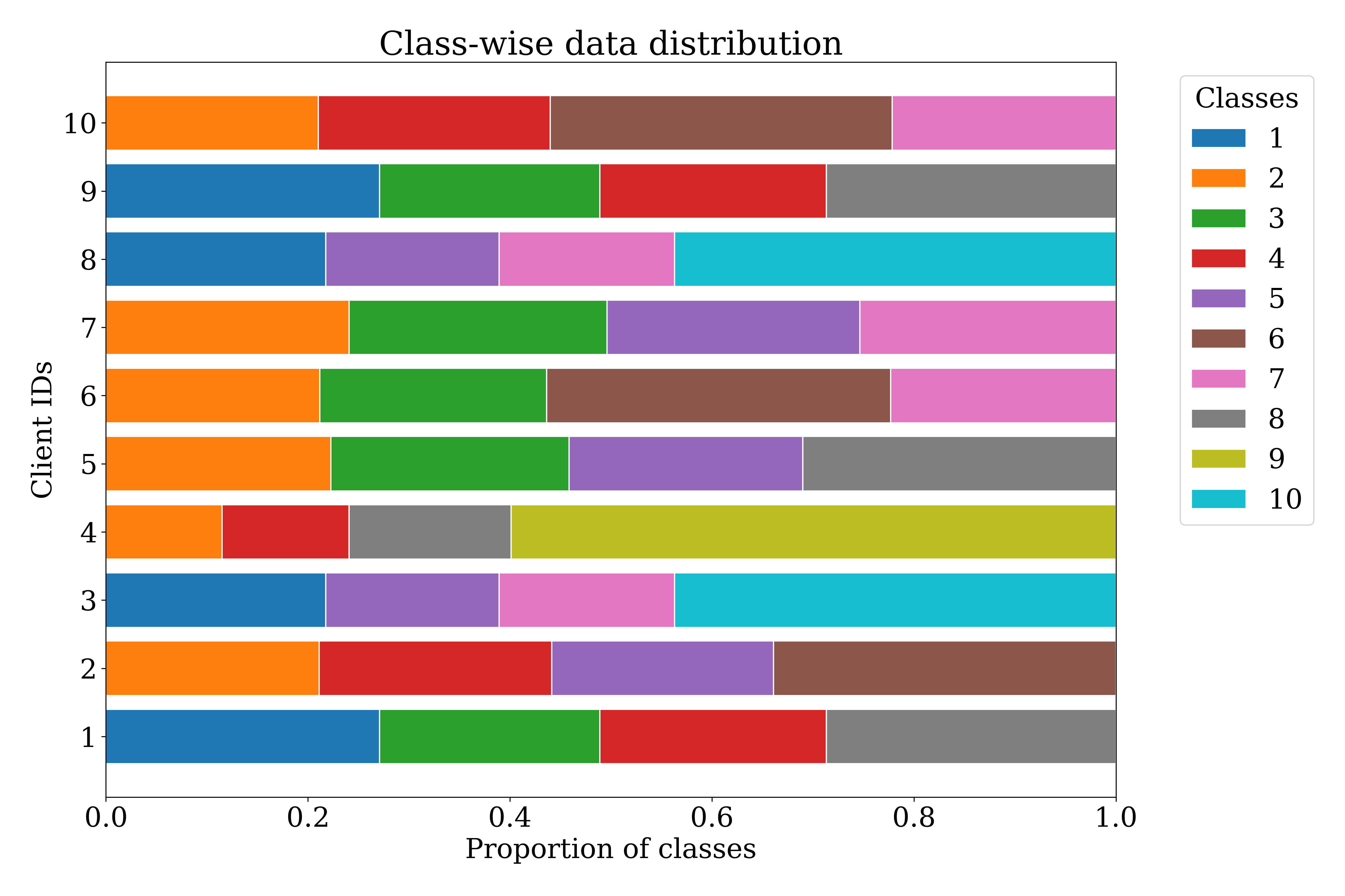
Figure 6: Non-IID Class Distribution for MNIST (Section 7) and CIFAR-10: Each client has four classes.

G.1 Heterogeneity between remaining and unlearned clients

This section investigates the stability in FU under varying levels of heterogeneity between these two groups, and data within both remaining and unlearned clients is homogeneous. According to Lemma 6.8, this setting should facilitate fairness in the unlearning process. Specifically, the number of classes in clients’ datasets follows a Dirichlet distribution with parameter $\alpha$, where a lower $\alpha$ value indicates higher data heterogeneity. We explore scenarios with $\alpha$ values corresponding to label distributions of 0.1, 0.4, and 0.7.

Table 2: Data Heterogeneity Between Groups ($P_{J}=0.38$): A lower label distribution indicates higher heterogeneity. Greater heterogeneity leads to increased instability after FU (evidenced by larger $S_{\text{retrain}}$ values). Employing a stability trade-off FU approach with $\lambda=1$ enhances stability (reduced $S_{\lambda=1}$) while maintaining negligible compromise in FU verification ($V_{\lambda=1}$).

Label Distribution	$S_{\text{retrain}}$	$S_{\lambda=1}$	$V_{\lambda=1}$
0.1	8.24	7.69 (-0.55)	0.0
0.4	3.45	2.05 (-1.4)	0.0
0.7	0.26	0.23 (-0.03)	0.06

Table 2 demonstrates a correlation between the data heterogeneity level and the system’s stability after unlearning.

A higher data heterogeneity leads to increased instability after unlearning, as indicated by the higher $S_{\text{retrain}}$ values. Notably, applying our FU mechanism with a stability trade-off parameter ($\lambda=1$) results in improved stability, as shown by the reduced $S_{\lambda=1}$ values, while the difference in FU verification remains negligible. This underscores our proposed approach could balance the trade-off between unlearning verification and global stability under varying degrees of data heterogeneity.

To further verify the unlearning, we examine the accuracy for class 4, which is unique to the unlearned clients. In the original trained model $\boldsymbol{\boldsymbol{w}}^{o}$, we observe a 77.09% accuracy for class 4. However, in the retrained model $\boldsymbol{w}^{r}$, the accuracy for class 4 drops to 0%, indicating successful unlearning. In our FU mechanism with stability penalty $\lambda=1$, the accuracy for class 4 is 0.3%, further validating the effectiveness of our approach in unlearning the influence of unlearned clients while maintaining stability.

G.2 Heterogeneity among remaining clients.

This section explores the fairness in FU under varying levels of heterogeneity among remaining clients, and data between remaining and unlearned clients is also heterogeneous.

To extend our analysis, we consider the CIFAR-10 dataset (Krizhevsky, 2009) with class distribution in Figure 6 and utilize the ResNet18 architecture (He et al., 2016). CIFAR-10 exhibits greater complexity compared to MNIST. Figure 7 illustrates the impact of unlearning on fairness among remaining clients, with a fairness parameter $\Lambda=1,\epsilon=20$. In this scenario, clients [1, 3] experienced significant utility loss due to their similar data distribution with unlearned clients [8, 9] (as shown in Figure 6). However, our FU mechanism achieves a lower fairness metric ($Q_{\text{our}}=6.91$) compared to the retraining approach ($Q_{\text{retrain}}=10.23$), indicating more equitable utility changes among remaining clients. The verification metric in this case is $V=0.42$, demonstrating that our mechanism enhances fairness even in more complex and heterogeneous environments.

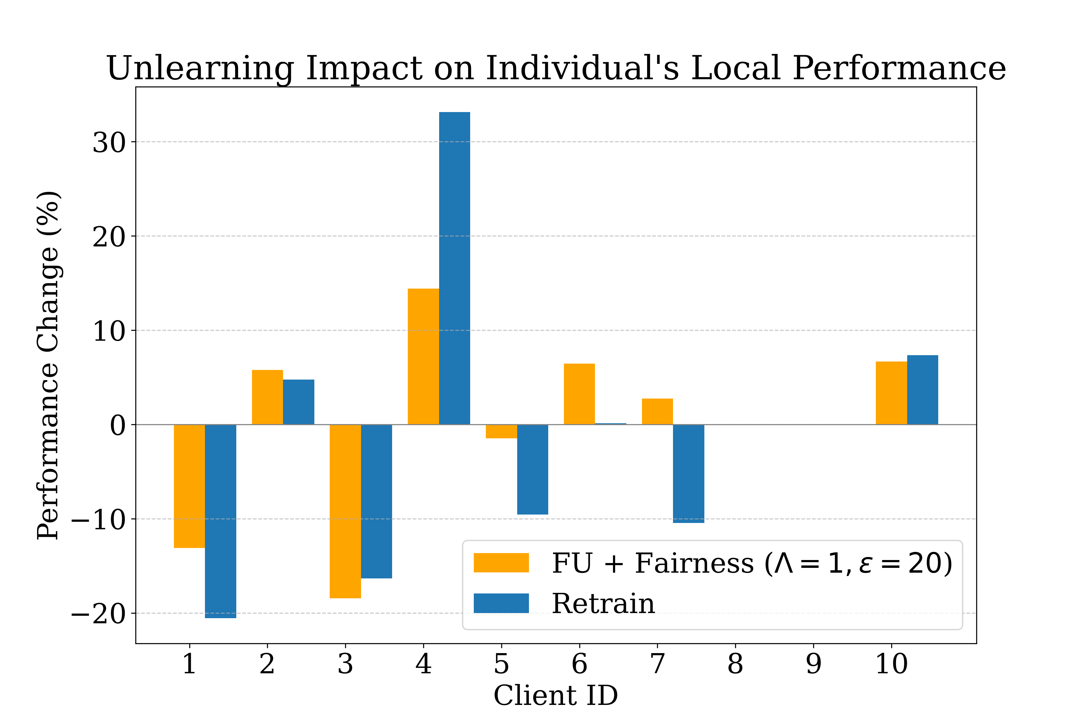
Figure 7: Unlearning Impact on Fairness: ensuring no client’s performance deviates beyond $20\%$; fairness metric ($Q$) of our FU mechanism ($Q_{\text{our}}=6.91$) is lower than that of retrain $Q_{\text{retrain}}=10.23$

References

- Agarwal et al. (2018) Alekh Agarwal, Alina Beygelzimer, Miroslav Dudík, John Langford, and Hanna Wallach. A reductions approach to fair classification. In International conference on machine learning, pp. 60–69. PMLR, 2018.
- Bourtoule et al. (2021a) Lucas Bourtoule, Varun Chandrasekaran, Christopher A. Choquette-Choo, Hengrui Jia, Adelin Travers, Baiwu Zhang, David Lie, and Nicolas Papernot. Machine unlearning. In 2021 IEEE Symposium on Security and Privacy (SP), pp. 141–159, 2021a. doi: 10.1109/SP40001.2021.00019.
- Bourtoule et al. (2021b) Lucas Bourtoule, Varun Chandrasekaran, Christopher A Choquette-Choo, Hengrui Jia, Adelin Travers, Baiwu Zhang, David Lie, and Nicolas Papernot. Machine unlearning. In 2021 IEEE Symposium on Security and Privacy (SP), pp. 141–159. IEEE, 2021b.
- Cao & Yang (2015) Yinzhi Cao and Junfeng Yang. Towards making systems forget with machine unlearning. In 2015 IEEE symposium on security and privacy, pp. 463–480. IEEE, 2015.
- Che et al. (2023) Tianshi Che, Yang Zhou, Zijie Zhang, Lingjuan Lyu, Ji Liu, Da Yan, Dejing Dou, and Jun Huan. Fast federated machine unlearning with nonlinear functional theory. In International conference on machine learning, pp. 4241–4268. PMLR, 2023.
- Ezzeldin et al. (2023) Yahya H. Ezzeldin, Shen Yan, Chaoyang He, Emilio Ferrara, and A. Salman Avestimehr. Fairfed: Enabling group fairness in federated learning. Proceedings of the AAAI Conference on Artificial Intelligence, 37(6):7494–7502, Jun. 2023. doi: 10.1609/aaai.v37i6.25911. URL https://ojs.aaai.org/index.php/AAAI/article/view/25911.
- Fang et al. (2020) Minghong Fang, Xiaoyu Cao, Jinyuan Jia, and Neil Gong. Local model poisoning attacks to Byzantine-Robust federated learning. In 29th USENIX security symposium (USENIX Security 20), pp. 1605–1622, 2020.
- Fraboni et al. (2022) Yann Fraboni, Martin Van Waerebeke, Kevin Scaman, Richard Vidal, Laetitia Kameni, and Marco Lorenzi. Sequential informed federated unlearning: Efficient and provable client unlearning in federated optimization. arXiv preprint arXiv:2211.11656, 2022.
- Gao et al. (2022) Xiangshan Gao, Xingjun Ma, Jingyi Wang, Youcheng Sun, Bo Li, Shouling Ji, Peng Cheng, and Jiming Chen. VeriFi: Towards Verifiable Federated Unlearning, May 2022. URL http://arxiv.org/abs/2205.12709. arXiv:2205.12709 [cs].
- Goldman (2020) Eric Goldman. An introduction to the california consumer privacy act (ccpa). Santa Clara Univ. Legal Studies Research Paper, 2020.
- Gu et al. (2022) Xiuting Gu, Zhu Tianqing, Jie Li, Tao Zhang, Wei Ren, and Kim-Kwang Raymond Choo. Privacy, accuracy, and model fairness trade-offs in federated learning. Comput. Secur., 122(C), nov 2022. ISSN 0167-4048. doi: 10.1016/j.cose.2022.102907. URL https://doi.org/10.1016/j.cose.2022.102907.
- Guo et al. (2020) Chuan Guo, Tom Goldstein, Awni Hannun, and Laurens Van Der Maaten. Certified data removal from machine learning models. In International Conference on Machine Learning, pp. 3832–3842. PMLR, 2020.
- Halimi et al. (2022) Anisa Halimi, Swanand Kadhe, Ambrish Rawat, and Nathalie Baracaldo. Federated unlearning: How to efficiently erase a client in fl? arXiv preprint arXiv:2207.05521, 2022.
- Hao et al. (2021) Weituo Hao, Mostafa El-Khamy, Jungwon Lee, Jianyi Zhang, Kevin J Liang, Changyou Chen, and Lawrence Carin Duke. Towards fair federated learning with zero-shot data augmentation. In Proceedings of the IEEE/CVF Conference on Computer Vision and Pattern Recognition, pp. 3310–3319, 2021.
- He et al. (2016) Kaiming He, Xiangyu Zhang, Shaoqing Ren, and Jian Sun. Deep residual learning for image recognition. In Proceedings of the IEEE conference on computer vision and pattern recognition, pp. 770–778, 2016.
- Hu et al. (2022) Shengyuan Hu, Zhiwei Steven Wu, and Virginia Smith. Fair federated learning via bounded group loss. arXiv preprint arXiv:2203.10190, 2022.
- Jia et al. (2023) Jinghan Jia, Jiancheng Liu, Parikshit Ram, Yuguang Yao, Gaowen Liu, Yang Liu, Pranay Sharma, and Sijia Liu. Model sparsification can simplify machine unlearning. arXiv preprint arXiv:2304.04934, 2023.
- Jin et al. (2023) Ruinan Jin, Minghui Chen, Qiong Zhang, and Xiaoxiao Li. Forgettable federated linear learning with certified data removal, 2023.
- Kairouz et al. (2021) Peter Kairouz, H Brendan McMahan, Brendan Avent, Aurélien Bellet, Mehdi Bennis, Arjun Nitin Bhagoji, Kallista Bonawitz, Zachary Charles, Graham Cormode, Rachel Cummings, et al. Advances and open problems in federated learning. Foundations and Trends® in Machine Learning, 14(1–2):1–210, 2021.
- Krizhevsky (2009) Alex Krizhevsky. Learning multiple layers of features from tiny images. Technical report, 2009.
- (21) Yann LeCun, Corinna Cortes, and CJ Burges. Mnist handwritten digit database.
- LeCun et al. (1998) Yann LeCun, Léon Bottou, Yoshua Bengio, and Patrick Haffner. Gradient-based learning applied to document recognition. Proceedings of the IEEE, 86(11):2278–2324, 1998.
- Li et al. (2023) Baochun Li, Ningxin Su, Chen Ying, and Fei Wang. Plato: An open-source research framework for production federated learning. In Proceedings of the ACM Turing Award Celebration Conference-China 2023, pp. 1–2, 2023.
- Li et al. (2019) Tian Li, Maziar Sanjabi, Ahmad Beirami, and Virginia Smith. Fair resource allocation in federated learning. arXiv preprint arXiv:1905.10497, 2019.
- Li et al. (2020a) Tian Li, Maziar Sanjabi, Ahmad Beirami, and Virginia Smith. Fair resource allocation in federated learning. In 8th International Conference on Learning Representations, ICLR 2020, Addis Ababa, Ethiopia, April 26-30, 2020. OpenReview.net, 2020a. URL https://openreview.net/forum?id=ByexElSYDr.
- Li et al. (2021) Tian Li, Shengyuan Hu, Ahmad Beirami, and Virginia Smith. Ditto: Fair and robust federated learning through personalization. In International Conference on Machine Learning, pp. 6357–6368. PMLR, 2021.
- Li et al. (2020b) Xiang Li, Kaixuan Huang, Wenhao Yang, Shusen Wang, and Zhihua Zhang. On the convergence of fedavg on non-iid data. In 8th International Conference on Learning Representations, ICLR 2020, Addis Ababa, Ethiopia, April 26-30, 2020. OpenReview.net, 2020b. URL https://openreview.net/forum?id=HJxNAnVtDS.
- Liu et al. (2022a) Bo Liu, Qiang Liu, and Peter Stone. Continual learning and private unlearning. In Sarath Chandar, Razvan Pascanu, and Doina Precup (eds.), Proceedings of The 1st Conference on Lifelong Learning Agents, volume 199 of Proceedings of Machine Learning Research, pp. 243–254. PMLR, 22–24 Aug 2022a. URL https://proceedings.mlr.press/v199/liu22a.html.
- Liu et al. (2020) Gaoyang Liu, Xiaoqiang Ma, Yang Yang, Chen Wang, and Jiangchuan Liu. Federated unlearning. arXiv preprint arXiv:2012.13891, 2020.
- Liu et al. (2021) Gaoyang Liu, Xiaoqiang Ma, Yang Yang, Chen Wang, and Jiangchuan Liu. FedEraser: Enabling Efficient Client-Level Data Removal from Federated Learning Models. In 2021 IEEE/ACM 29th International Symposium on Quality of Service (IWQOS), pp. 1–10, June 2021. doi: 10.1109/IWQOS52092.2021.9521274. ISSN: 1548-615X.
- Liu et al. (2022b) Yi Liu, Lei Xu, Xingliang Yuan, Cong Wang, and Bo Li. The right to be forgotten in federated learning: An efficient realization with rapid retraining. In IEEE INFOCOM 2022-IEEE Conference on Computer Communications, pp. 1749–1758. IEEE, 2022b.
- McMahan et al. (2017) Brendan McMahan, Eider Moore, Daniel Ramage, Seth Hampson, and Blaise Aguera y Arcas. Communication-Efficient Learning of Deep Networks from Decentralized Data. In Aarti Singh and Jerry Zhu (eds.), Proceedings of the 20th International Conference on Artificial Intelligence and Statistics, volume 54 of Proceedings of Machine Learning Research, pp. 1273–1282. PMLR, 20–22 Apr 2017. URL https://proceedings.mlr.press/v54/mcmahan17a.html.
- Mohri et al. (2019) Mehryar Mohri, Gary Sivek, and Ananda Theertha Suresh. Agnostic Federated Learning. In Proceedings of the 36th International Conference on Machine Learning, pp. 4615–4625. PMLR, May 2019. URL https://proceedings.mlr.press/v97/mohri19a.html. ISSN: 2640-3498.
- Nguyen et al. (2022) Thanh Tam Nguyen, Thanh Trung Huynh, Phi Le Nguyen, Alan Wee-Chung Liew, Hongzhi Yin, and Quoc Viet Hung Nguyen. A Survey of Machine Unlearning, October 2022. URL http://arxiv.org/abs/2209.02299. arXiv:2209.02299 [cs].
- Pan et al. (2023a) Chao Pan, Jin Sima, Saurav Prakash, Vishal Rana, and Olgica Milenkovic. Machine unlearning of federated clusters. In The Eleventh International Conference on Learning Representations, ICLR 2023, Kigali, Rwanda, May 1-5, 2023. OpenReview.net, 2023a. URL https://openreview.net/pdf?id=VzwfoFyYDga.
- Pan et al. (2023b) Zibin Pan, Shuyi Wang, Chi Li, Haijin Wang, Xiaoying Tang, and Junhua Zhao. Fedmdfg: Federated learning with multi-gradient descent and fair guidance. In Proceedings of the AAAI Conference on Artificial Intelligence, volume 37, pp. 9364–9371, 2023b.
- Regulation (2018) General Data Protection Regulation. General data protection regulation (gdpr). Intersoft Consulting, Accessed in October, 24(1), 2018.
- Shi et al. (2023) Yuxin Shi, Han Yu, and Cyril Leung. Towards fairness-aware federated learning. IEEE Transactions on Neural Networks and Learning Systems, 2023.
- Tarun et al. (2023a) Ayush K. Tarun, Vikram S. Chundawat, Murari Mandal, and Mohan Kankanhalli. Fast yet effective machine unlearning. IEEE Transactions on Neural Networks and Learning Systems, pp. 1–10, 2023a. doi: 10.1109/tnnls.2023.3266233. URL https://doi.org/10.1109%2Ftnnls.2023.3266233.
- Tarun et al. (2023b) Ayush Kumar Tarun, Vikram Singh Chundawat, Murari Mandal, and Mohan S. Kankanhalli. Deep regression unlearning. In Andreas Krause, Emma Brunskill, Kyunghyun Cho, Barbara Engelhardt, Sivan Sabato, and Jonathan Scarlett (eds.), International Conference on Machine Learning, ICML 2023, 23-29 July 2023, Honolulu, Hawaii, USA, volume 202 of Proceedings of Machine Learning Research, pp. 33921–33939. PMLR, 2023b. URL https://proceedings.mlr.press/v202/tarun23a.html.
- Wang et al. (2023) Fei Wang, Baochun Li, and Bo Li. Federated unlearning and its privacy threats. IEEE Network, 2023.
- Wang et al. (2021) Jianyu Wang, Zachary Charles, Zheng Xu, Gauri Joshi, H Brendan McMahan, Maruan Al-Shedivat, Galen Andrew, Salman Avestimehr, Katharine Daly, Deepesh Data, et al. A field guide to federated optimization. arXiv preprint arXiv:2107.06917, 2021.
- Wang et al. (2020) Tianhao Wang, Johannes Rausch, Ce Zhang, Ruoxi Jia, and Dawn Song. A principled approach to data valuation for federated learning. Federated Learning: Privacy and Incentive, pp. 153–167, 2020.
- Wu et al. (2022) Chen Wu, Sencun Zhu, and Prasenjit Mitra. Federated unlearning with knowledge distillation. arXiv preprint arXiv:2201.09441, 2022.
- Wu et al. (2020) Yinjun Wu, Edgar Dobriban, and Susan B. Davidson. Deltagrad: Rapid retraining of machine learning models. In Proceedings of the 37th International Conference on Machine Learning, ICML 2020, 13-18 July 2020, Virtual Event, volume 119 of Proceedings of Machine Learning Research, pp. 10355–10366. PMLR, 2020. URL http://proceedings.mlr.press/v119/wu20b.html.
- Yang & Zhao (2023) Jiaxi Yang and Yang Zhao. A survey of federated unlearning: A taxonomy, challenges and future directions, 2023.
- Yin et al. (2018) Dong Yin, Yudong Chen, Ramchandran Kannan, and Peter Bartlett. Byzantine-robust distributed learning: Towards optimal statistical rates. In International Conference on Machine Learning, pp. 5650–5659. PMLR, 2018.
- Yu et al. (2020) Han Yu, Zelei Liu, Yang Liu, Tianjian Chen, Mingshu Cong, Xi Weng, Dusit Niyato, and Qiang Yang. A fairness-aware incentive scheme for federated learning. In Proceedings of the AAAI/ACM Conference on AI, Ethics, and Society, pp. 393–399, 2020.
- Zhang et al. (2023) Lefeng Zhang, Tianqing Zhu, Haibin Zhang, Ping Xiong, and Wanlei Zhou. Fedrecovery: Differentially private machine unlearning for federated learning frameworks. IEEE Transactions on Information Forensics and Security, 2023.