Characteristics of the Alfvénic activity during the current quench in ASDEX Upgrade

Abstract

ASDEX Upgrade has developed multiple massive gas injection (MGI) scenarios to investigate runaway electron (RE) dynamics. During the current quench of the MGI induced disruptions, Alfvénic activity is observed in the 300–800 kHz range. With the help of a mode tracing algorithm based on Fourier spectrograms, mode behaviour was classified for 180 discharges. The modes have been identified as global Alfvén eigenmodes using linear gyrokinetic MHD simulations. Changes in the Alfvén continuum during the quench are proposed as explanation for the strong frequency sweep observed. A systematic statistical analysis shows no significant connection of the mode characteristics to the dynamics of the subsequent runaway electron beams. In our studies, the appearance and amplitude of the modes does not seem to affect the potential subsequent runaway beam. Beyond the scope of the 180 investigated dedicated RE experiments, the Alfvénic activity is also observed in natural disruptions with no RE beam forming.

1 Introduction

Widely used techniques for disruption mitigation in tokamaks include massive gas injection (MGI) [1, 2, 3] and shattered pellet injection (SPI) [4, 5]. Hereby, a large amount of material is injected into the plasma as gas puff or as frozen pellet fragments, respectively. Even though there has been significant progress on the physics basis and design of the ITER disruption mitigation system (DMS) [6, 4, 5, 7, 8], effective disruption mitigation for the next generation of fusion devices such as ITER or DEMO remains a challenging task [9, 10, 11]. In particular, developing a robust runaway electron (RE) mitigation technique for an activated wall phase with nuclear primary runaway electron sources has been proven difficult [12, 13]. A beam of runaway electrons with multi-MeV energies rises due to high toroidal electric fields induced during a disruption [14]. Even a small seed of REs can self-amplify due to collisions between the fast seed electrons and the bulk, leading to an avalanche effect [15, 16]. Ideally, disruption mitigation scenarios aim to avoid the formation of high-current RE beams, which can cause severe damage to the machine [17].

The benign termination of the RE beam [18, 19, 20] is a promising candidate for a mitigation technique. Plasma waves might contribute to the avoidance of the formation of strong RE beams, as the level of magnetic perturbations [21] and Alfvénic activity in post-disruption plasmas [22, 23] can have a strong influence on a subsequent runaway current formation. In the contributions by Lvovskiy et al. [24, 25], they present instabilities observed during disruptions in the tokamak DIII-D, which could deconfine the initial seed electrons, hence suppressing the formation of a strong RE beam.

In this paper we present a detailed investigation on post-disruption modes observed in the tokamak ASDEX Upgrade (AUG). We discuss mode characteristics, different statistical analysis techniques as well as simulation results. The modes described in this paper were identified as global Alfvén eigenmodes (GAEs). The paper is organised as follows. In section 2 the setup and discharge parameters of the experiments are described. The tracing algorithm used for the analysis is detailed in section 3. The observations and results of the mode tracing are discussed in section 4. Section 5 presents the mode classification results. Section 6 covers the statistical analysis of the modes. Simulation analysis of the mode characteristics is presented in section 7.

2 Experimental dataset

The database analysed in this paper consists of 180 ASDEX Upgrade discharges conducted with the primary goal of runaway electron generation. It ranges from shot number #31318 (July 2014) to #38088 (July 2020). The discharges are all inner wall limited, circular plasmas (elongation $\kappa\approx 1.1$) [3]. A summary of global parameters for these discharges is shown in table 1.

Table 1: Global parameter ranges for the discharges in the database. The numbers inside the parentheses represent the number of discharges within this parameter range, with a total of 180.

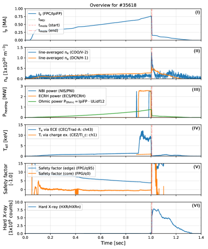
(a) Typical RE scenario with trigger of the MGI valve at t = 1.0 s.

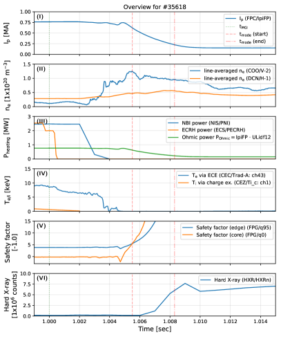
(b) Zoom of (a) with mode activity time window highlighted.

Figure 1: Reference discharge #35618 as a representative shot for the discharges within the database. The plasma current in (I), line-averaged electron density from interferometry (II), heating powers (III), electron (core Electron Cyclotron Emission – ECE) and ion temperatures (CXRS) (IV), edge/core safety factors (V), and hard X-ray count (VI) are given. In the zoomed-in version in (b), the time window of the mode for this discharge is also highlighted.

In figure 1 the temporal evolution of the reference discharge of this paper (#35618) is indicated. We divide the discharges into three phases. The first phase is the current ramp-up, leading to the pre-timed massive gas injection. During the first second of the discharge the plasma current ($I_{\textnormal{p}}$) is ramped up to values typically around 800 kA and the target density (pre-disruption plasma density $n_{\textnormal{pre}}$ or electron density $n_{\textnormal{e}}$) is around $3\cdot 10^{19}\ \textrm{m}^{-3}$. At around $t=1.00\ \textrm{s}$, an in-vessel massive gas injection [1, 2, 3] is triggered, which leads to the intended disruption. Most of the cases feature argon injection at different gas pressures, with a minority of the shots testing neon or krypton injection. The discharges typically do not reach flat-top and are disrupted during the ramp-up phase. This is motivated by two reasons: to increase the chance of runaway generation via the presence of the ramp-up loop voltage, and to preempt the potential formation of locked modes due to the relatively low density operation. The exact injection timing slightly varied for 20 of the 180 discharges inside the database. The reason for this variation is a scan of pre-disruption plasma current. Disrupting the ramp-up at different times leads to runaway formation from different starting currents, while keeping the same loop voltage during the ramp-up and at the time of the injection. Core Electron Cyclotron Resonance Heating (ECRH) heating is applied in some cases 100 ms before the timed MGI to facilitate RE generation and to provide a core temperature scan. Additionally, a Neutral Beam Injection (NBI) blip was applied to enable the measurements of beam diagnostics like Charge Exchange Recombination Spectroscopy (CXRS) (see ion temperature $T_{\textnormal{i}}$ measurement in figure 1).

To achieve reliable runaway beam formation, most of the time argon is used as MGI gas – in this database 166 out of 180 discharges (see table 1). Argon quantities injected vary between $3\cdot 10^{20}$ and $4.8\cdot 10^{21}$ atoms. In the second phase, the injected gas penetrates the plasma and starts to radiate away the previously confined energy [26]. Within a few milliseconds the plasma cools down from around 10 keV of core temperature to a few eV, followed by the current quench, discussed in more detail in section 4.

As the experiments were designed to investigate runaway electron generation [2, 3], the last phase of the discharges is mostly characterised by the presence of a RE plateau. Around 77% of the discharges in the set show a runaway current above 50 kA. For plasma currents below this value plasma position control is difficult and the shot typically ends in a VDE. A more detailed description of the scenario and these experiments is given in the papers by Pautasso et al. [2, 3].

Of the 180 discharges in this dataset, virtually all of them have shown signatures of Alfvénic frequency modes in the current quench. The magnetic pick-up coils (Mirnov- and Ballooning coils) of ASDEX Upgrade [27, 28, 29] are well suited to measure the frequency evolution of the post-disruption modes. The pick-up coils have a sampling frequency of 2 MHz, setting the maximum measurable mode frequency at 1 MHz. While the data acquisition system allows for setting the sampling frequency to 10 MHz for short time intervals, this was not routinely applied.

3 Mode tracing

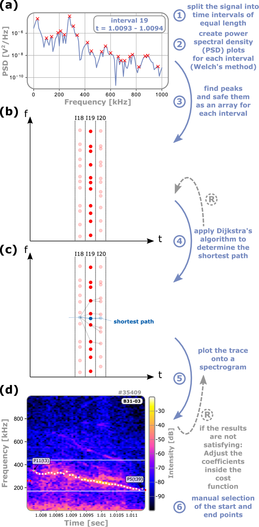
Figure 2: Concept of the mode tracing algorithm.

In order to automatically characterise the amplitude and frequency evolution of the modes observed during the current quench, we developed a mode tracing algorithm [30]. The main idea of this algorithm is shown in figure 2 and briefly summarised in the following.

1. The signal is divided into time intervals of equal length. We used 40 time intervals, which results in a sampling into 40 time-frequency points. This “downsampling” is used to reduce computational time.

2. For each interval, the power spectral density (PSD) is calculated via Welch’s method shown in figure 2(a).

3. A local peak finding algorithm is applied to create an array of frequencies representing the time evolution of the mode frequency.

4. The grid necessary to apply Dijkstra’s algorithm is initialised. Thereby, each frequency point (node) from interval $i$ is connected to each other node from interval $i+1$ if the change in frequency $\Delta f<\Delta f_{\textnormal{max}}$ is less than a predefined maximum jump frequency. For this values between 0.4 and 6 kHz $\cdot$ 1s/($\Delta t_{i\rightarrow i+1}$ in s) were used where 1 kHz was the default setting used in 75 cases. The first and the last interval are connected to only a single “artificial” node, which act as the start and end points, respectively. To every connection between nodes (vertex) a value is assigned via the cost function

   $$\textnormal{cost}(i\rightarrow i+1)=c_{f}\cdot\Delta f+\frac{c_{A}}{A_{i+1}},$$ (1)

   with user defined weighting coefficients $c_{f}$ and $c_{A}$ as well as the absolute amplitude $A_{i+1}$ measured for the second node in the node-vertex-node connection as suggested by Magyarkuti [31]. Ratios for $c_{f}$:$c_{A}$ between 10:125 and 500:10 were applied, however, a 1:1 ratio was used in 104 cases. Now Dijkstra’s algorithm can be applied on this map, which yields the path with the global lowest cost from the start to the end node with one node per interval.

5. The result is plotted on top of a high-resolution spectrogram (white points in 2(d)). If the result is not satisfactory, new values for $c_{f}$, $c_{A}$ and $\Delta f_{\textnormal{max}}$ may be selected and the steps – are repeated.

6. When the results are satisfactory, the user can select the start and end points manually in the graphical user interface.

4 General mode characteristics

In this section we are going to discuss general characteristics of the observed modes, such as time-frequency evolution, mode structure, and the time interval in which these appear.

As illustration, the plasma current ($I_{\textnormal{p}}$) evolution around the quench phase for discharge #35618 is displayed in figure 3(a). The MGI was triggered at 1.000 seconds, and within a few milliseconds the thermal quench (TQ) occurs. After the $\textnormal{I}_{\textnormal{p}}$ spike [32] the plasma current collapses during the current quench (CQ) phase, followed by the RE plateau with initial runaway current around 156 kA.

fig1.4

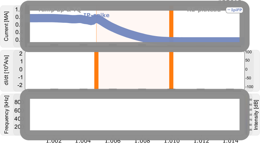
Figure 3: Definition of the CQ time window for the scope of this work. In (a) the evolution of the plasma current is given, with its temporal derivative depicted in (b). In (c) a spectrogram for the magnetic coil B31-03 is provided, which shows the presence of a sweeping mode.

The d$I_{\textnormal{p}}$/dt temporal derivative of the plasma current is shown in figure 3(b). For our definition, the initial $\textnormal{I}_{\textnormal{p}}$ spike marks the start of the CQ, located at the zero-crossing of the temporal derivative. It lasts until the change in plasma current approaches zero again. For the scale on the right in figure 3(b), the temporal derivative of the current is normalised to its maximum value. As the consecutive RE plateaus also show a slight decay over time, a threshold at -0.25% normalised d$I_{\textnormal{p}}$/d$t$ was applied to all discharges to determine a quantitatively reproducible end point of the current quenches.

In figure 3(c) the spectrogram for the radial magnetic field perturbation coil B31-03 is shown. It is located at the low field side midplane and was used as a reference coil for most of the discharges. The spectrogram shows the presence of a mode sweeping from around 800 to 400 kHz between 1.006 to 1.008 seconds, during the current quench.

Figure 4 is a summary plot of mode evolution in all investigated discharges. The figure shows the frequency evolution – obtained by the mode tracing algorithm discussed in section 3 – of all modes against time normalised to the current quench time window. Colours indicate the different sweeping behaviours which will be detailed in section 5. Discharge #35618 is highlighted as a reference.

While the individual mode evolutions can differ between the discharges, they nevertheless display similar general behaviour. As shown in figure 4, the time traces of the modes are located exclusively during the current quench phase. For this reason, the modes will be referred to as current quench modes (CQ mode) within this paper.

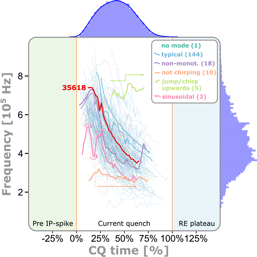
Figure 4: Time window of CQ mode evolution. The mode frequency traces are plotted as function of time normalised to current quench duration. The modes are located exclusively inside the CQ. The temporal evolution for the reference discharge #35618 as well as examples for each category are highlighted.

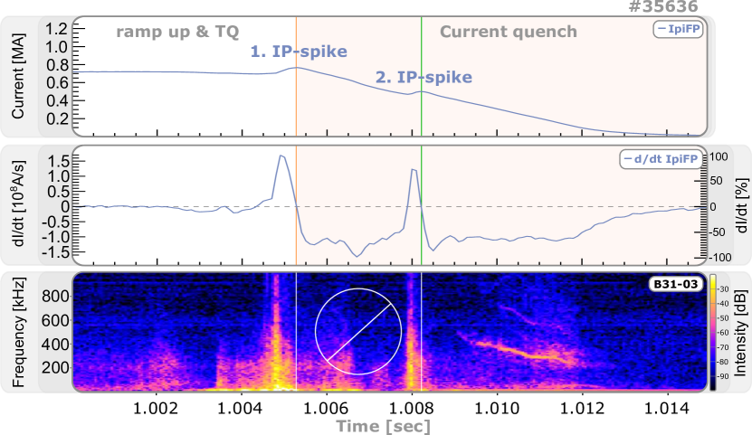
Figure 5: Behaviour of the modes in multi-stage disruptions. The mode always appears after the last $\textnormal{I}_{\textnormal{p}}$ spike has occurred.

Our database includes five discharges, which show incomplete disruptions, i.e. multiple $\textnormal{I}_{\textnormal{p}}$ spikes appear. In figure 5(a) we observe a second $\textnormal{I}_{\textnormal{p}}$ spike about 3 ms after the first. As shown in the spectrogram, the mode is only present after the last $\textnormal{I}_{\textnormal{p}}$ spike has occurred. A similar trend is observed for the other “multi-stage” disruptions in the database. This indicates that the modes are not triggered by a drop of plasma current alone.

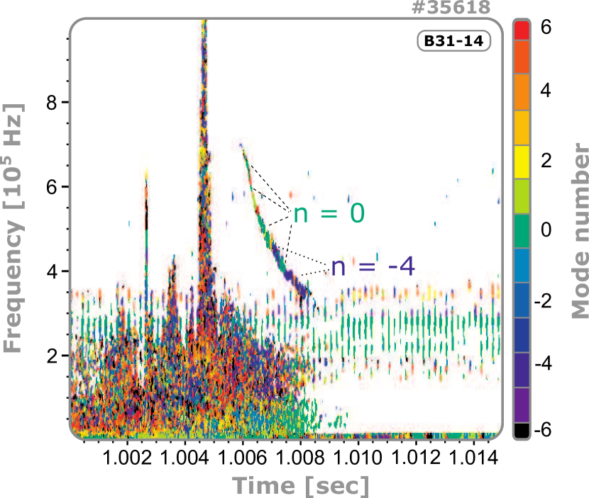
Figure 6: Analysis of the toroidal mode number n. The mode appears to be a mixture of many different mode numbers. The most prominent are $n=0$ and $n=-4$.

First investigations of the mode location – details provided in the thesis of P. Heinrich [30] – point towards strong mode amplitudes in the Soft X-ray channels closer to the separatrix. However, proper normalisation of the signals is highly complex. Therefore, this can only be interpreted as a first hint of the radial location of these modes. As ASDEX Upgrade is equipped with a large set of magnetic pick-up coils, distributed over the torus in poloidal and toroidal directions, one can calculate the poloidal (m) and toroidal (n) mode numbers [33, 29]. Figure 6 shows the toroidal mode number calculation for our reference discharge #35618. Even though the mode is globally coherent, it does not show a unique mode number (neither toroidal nor poloidal) for any of the investigated discharges, but rather a mix of many different ones as shown in the example. Based on the plots, the most prominent toroidal mode numbers are $n=0$ and $n=-4$. A negative $n$ value represents the propagation of the mode in the ion diamagnetic drift direction.

5 Classification of the CQ modes

During the investigations of the CQ modes, each of the 179 modes has been characterised and five different categories are identified. In the following a short description of the five characteristics is given.

5.1 Frequency sweeping

The most prominent characteristic of these modes is their frequency sweeping behaviour. As a mode evolves in time, its amplitude and frequency changes. This typically results in a frequency evolution, where the mode starts at higher frequencies – typically around 800 kHz – and sweeps towards lower frequencies (see figure 7(a)). The change in frequency is typically strongest at the beginning and reduces towards the end of the mode. This evolution is the most common type of sweeping behaviour as shown in the distribution in figure 8(a), thus is referred to as typical throughout this paper. Discharge #35618, representing this kind of sweeping behaviour, is used as a reference and was analysed in more detail, also with the help of simulations (see section 7).

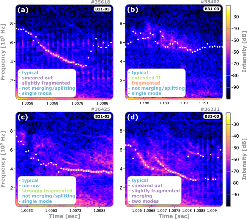
Figure 7: Comparison of different mode characteristics for the magnetic pick-up coil B31-03. The mode characteristics from figure 8 are given in the boxes for each example.

5.2 Mode contour

The spectral width of a mode is qualitatively classified as the sharpness of the mode contour. Cases exist – referred to as narrow – which depict a sharp contour, thus have a well defined frequency. The more the modes lose their sharp contour as the spectral width broadens, the harder it is to determine their main frequency. If the main frequency is hard to determine, as the mode does not show a distinct contour, the mode is referred to as extended (compare figure 7(b)). If at least a short fragment of the mode shows this behaviour but the rest is well traceable, it is labeled as extended I. In case the mode contour does not show the distinct contour but shows a trend that is visible (compare figure 7(b)) it is referred as extended II and in case this trend is not visible anymore as extended III.

5.3 Degree of fragmentation

Modes can also show fragmentation effects which are classified by the degree of fragmentation. It indicates, how continuously a mode evolves in time and how many intersections appear. The higher the degree of fragmentation, the harder it is to trace the amplitude and frequency evolution of the modes. This parameter also depends on the position of the magnetic coil. The distribution given in figure 8(c) shows the degree of fragmentation mainly for the reference coil B31-03. In a few cases better tracking precision can be achieved by using other pick-up coils or soft X-ray.

5.4 Merging & splitting of modes

In some discharges modes are present, which seem to split into two mode branches or emerge from them. Separate mode branches are only counted as a second mode if they are clearly separated. If two modes appear within a discharge, they mostly merge at a certain point in time (see figure 7(d)). For most discharges we observe no merging or splitting behaviour as shown in figure 8(d).

5.5 Number of modes

As shown in figure 8(e), in most discharges we observe single modes and often their upper harmonics. For this classification the number of harmonics is not taken into consideration, thus only the number of distinct modes was investigated. For 16 discharges in our database we observe two modes. Nearly all of them merge at a certain point in time – between approximately 30 – 55% of the total duration of merging modes. The only discharge, which seems not to contain any modes is #38074. Neither in the magnetics nor in the soft X-ray lines of sight (LOSs) any activity was observed. However, the global parameters do not show any prominent differences to the other discharges from the same session.

(a) Distribution of different sweeping behaviours.

(b) Distribution of different mode contours.

(c) Distribution of different degrees of fragmentation.

(d) Distribution of merging and splitting of modes.

(e) Distribution of number of modes which appear inside each discharge.

Figure 8: Distributions of the five mode characteristics with the total number inside the parentheses.

6 Statistical analysis

With the help of the mode time traces and characteristics, multiple statistical analysis methods had been applied and hypotheses tested. It was investigated whether different mode parameters (e.g. the above mentioned characteristics, the mode amplitude or duration) show an effect on the subsequent RE formation. In subsection 6.1, the results of a histogram based analysis to determine the modes’ most likely frequencies is given. A correlation matrix for 38 different observables was analysed in detail and the results are summarised in subsection 6.2. In subsection 6.3, the results from the factor analysis are presented, which aims to connect the observables of a system with underlying (hidden) factors. The results from hypothesis testing with the help of regressions are given in subsection 6.4.

6.1 Most likely frequency

In case the CQ modes have a significant effect on the formation of RE plateaus, a future external mode drive might become desirable. For the excitation of these waves, their resonance frequency has to be known in advance. Based on our database the so-called most likely frequency (MLF) for each discharge was determined. It represents the mode frequency, which is maintained for the longest duration. Introduced by the mode tracing algorithm, a time sampling of 40 time points is applied and the frequencies within 10 kHz-bins are counted. As these modes often sweep strongest at the start, the MLFs are not necessarily given by the arithmetic mean. Therefore, the individual MLF for each discharge was determined via histograms with a bin size of 10 kHz. For every discharge, the individual probability density function of the mode frequency was calculated. The MLF is determined by the global maximum of this distribution, thus the most probable frequency. The distribution of the 179 MLFs for each mode is shown in figure 9. The maxima are located at 340 and 370 kHz. Therefore, the most probable resonance frequency for externally driven modes is slightly below 400 kHz.

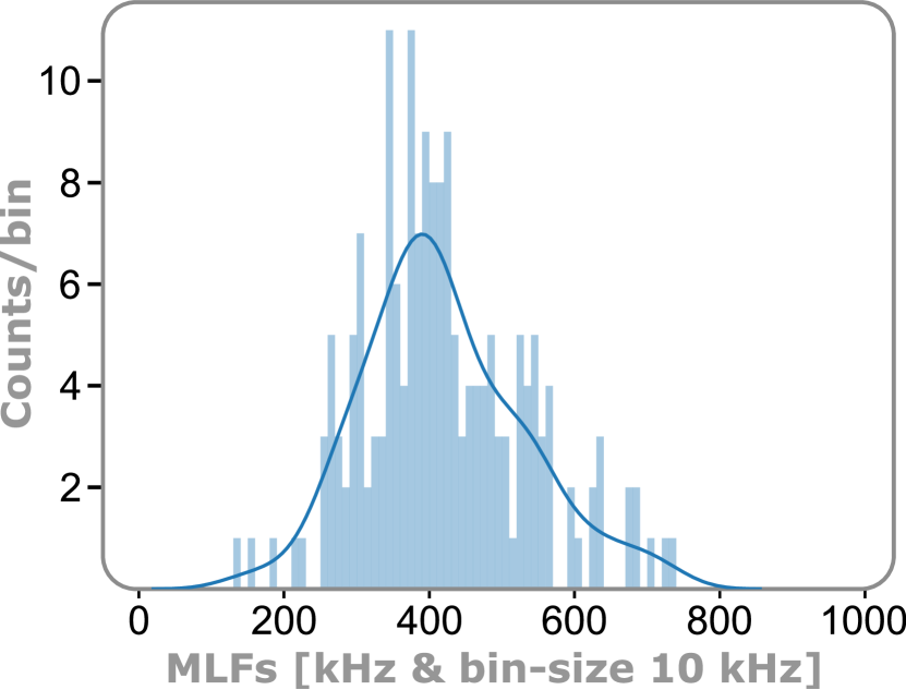
Figure 9: The distribution of the most likely frequencies (MLFs) of the modes is shown with maxima at 340 and 370 kHz.

6.2 Summary of the correlation matrix analysis

A correlation matrix for 38 observables was calculated and analyzed in detail. This includes for example the plasma and subsequent RE current, toroidal magnetic field strength, plasma temperature, the plasma safety factor at $\rho_{\textnormal{pol}}=0.95$ (q95) or density measurements. A detailed list and description for each observable as well as the correlation matrix itself is given in A.1 and 2. In the following the results of the analysis are presented. Most of the higher correlations between the plasma parameters can be explained by well known interactions (e.g. the connection of the plasma current with the plasma safety factor). In addition to those correlations two regions of special interest can be observed in the matrix. The relevant excerpt of this correlation matrix discussed in the following is provided in table 2.

Table 2: Excerpt of regions of interest in the correlation matrix given in A.1 and 2. The description for all quantities are available in the table in A.1. In bold, correlation values with an absolute value above 0.3 are presented. No strong correlation between mode characteristics defined in section 5 and global plasma/disruption parameters are observed.

6.2.1 Correlation between CQ- and mode-times with global plasma parameters (region 2)

In this first region of interest, the timing and length of the CQ and CQ modes are connected to global plasma parameters such as the (runaway) current, toroidal magnetic field strength, q95 and MGI gas quantity (compare row $\textnormal{dt}_{\textnormal{mode}}$ in table 2). The modes appear exclusively during the CQ as shown in section 4. For longer current quench and mode duration, a lower subsequent current is held by runaway electrons ($I_{\textnormal{RE}}$) and a higher change in current (d$I$) will be achieved as the current change rates (d$I_{\textnormal{p}}$/dt) are very similar between each shot. This results in high correlation values – positive (correlated) for the change in current, negative (anti-correlated) for the runaway current. Another observation of this region is the anti-correlation between the amount of gas injected to trigger the disruption ($\textnormal{N}_{\textnormal{Z}}$) with the CQ and mode times ($\textnormal{dt}_{\textnormal{CQ}}$ and $\textnormal{dt}_{\textnormal{mode}}$) as well as the start ($t_{\textnormal{IP}}-t_{\textnormal{trigger}}$) and end ($t_{\textnormal{end CQ}}-t_{\textnormal{trigger}}$) times of the current quench. More gas causes hereby shorter CQ time windows in which the mode can exist. The values for the safety factor $q_{95}$ are typically adjusted by varying the plasma current and toroidal magnetic field. As the pre-disruption plasma current is determined by the timing of the MGI, the trigger time shows strong correlations with the toroidal magnetic field component ($B_{\textnormal{tor}}$) and $q_{95}$. Thereby, earlier injections lead to lower initial plasma currents, hence higher safety factors by design.

6.2.2 Mode characteristics and global plasma parameters (region 4)

The region in the correlation matrix which connects the mode characteristics from section 5 with the global plasma parameters was the main focus of this investigation (excerpt given in table 2). A high correlation would point towards a connection between the mode behaviour and global parameters. However, we do not observe any significant correlations in this region. The subtle correlations within this regions can be explained due to the nature of the characterisation system used within the mode tracing algorithm [30]. Consequently, the mode characteristics and amplitudes do not seem to affect the – or being affected by – global plasma parameters.

6.3 Results from factor analysis

In this concept multiple observables of the system are reduced to a few underlying factors [34]. These factors are also often referred to as hidden variables as they are not directly measured, but their effect can be visible throughout the observables. A scree plot is used to determine how many factors are necessary to describe the underlying connections of the system. It visualizes the separation of high impact factors for the system, from the rest (”scree”). It typically shows a so-called elbow or inflection point depicted in figure 10(a), which acts as the desired separation between factors.

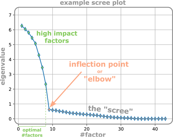
(a) Example scree plot showing an inflection point

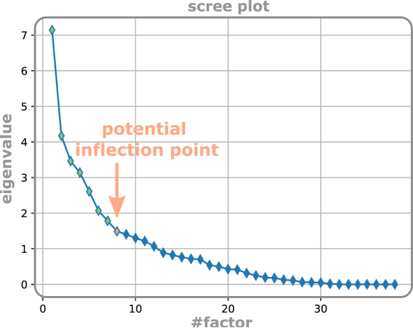
(b) Scree plot of the FA for the database.

Figure 10: In (a) an example for a typical scree plot is given. The inflection point separates the high impact factors from the ”scree”. In (b) the scree plot of the EFA for our database is depicted. It does not show a clear inflection point, being the usual, strong separation between factors. Factor 8 is highlighted as a potential inflection point.

In our case we used exploratory factor analysis (EFA) to find factors, which describe a possible interaction between global parameters and mode characteristics. The results presented in figures 10(b) and 11 were created with the python module FactorAnalyzer [35] with the rotation-mode varimax (more details in the documentation [35]). The scree plot in figure 10(b) does not show a distinct inflection point. This indicates, that the results could not be reduced to a few underlying factors. This could be due to the system being highly complex or the observables not being suited to describe the system well enough with only a few factors. The first 9 factors and their loadings (values indicating the effect of that variable on the factor) are shown in figure 11. Hereby, the factors are sorted by eigenvalues, thus their impact on the system. The factor analysis code can not provide a description or name for each factor. Consequently, we will refer to each factor by it’s number displayed at the top. A detailed analysis and interpretation for the loadings of each factor given in figure 11, is available in the A.3.

As a result of the analysis process, custom names for each factor are given in table 3. Our main focus was to analyse connections between mode characteristics and other observables via hidden variables of the system. However, also with this analysis technique, no significant connections have been observed. Most of the loadings were already expected due to prior knowledge of the physical dependencies or experimental setup, as indicated in the table 3. Again, higher loadings for the mode characteristics can be connected to the tracing and characterisation methods instead of physical phenomena.

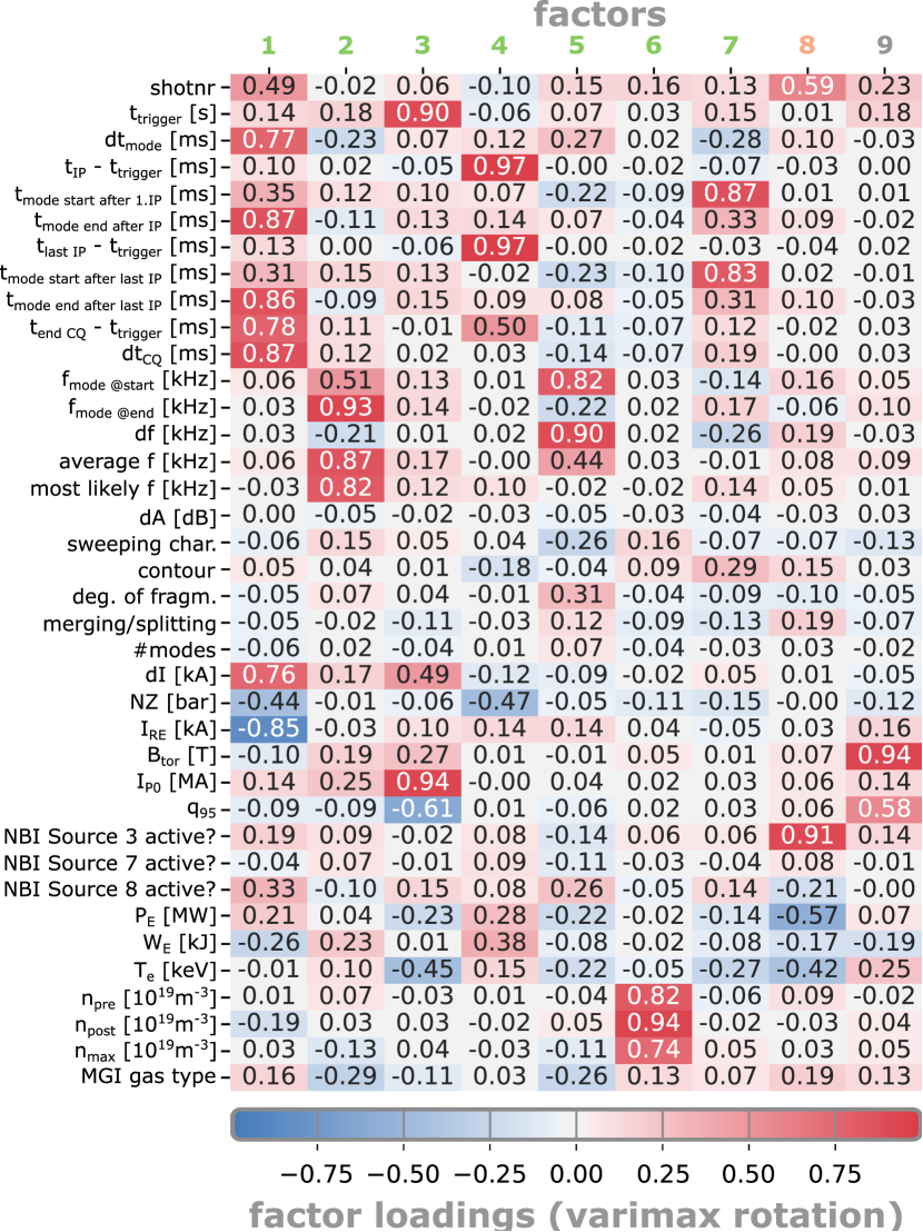
Figure 11: The loadings for the first 9 factors resulting from the factor analysis. A summarizing description for each factor is provided in table 3. The orange color of factor 8 is used to mark it as the potential weak inflection point.

Table 3: Potential custom names and description of the factors based on their loading.

6.4 Regressions

In the contribution by Lvovskiy et al. [24, 25], the duration of MHD activity and the loss of the initial RE seed are connected, thus the consequent runaway current $I_{\textnormal{RE}}$ is affected. To analyse this connection for ASDEX Upgrade, linear regressions are created. In figure 12(a) the RE current is shown against the duration of the current quench modes. The trend shows a decreasing runaway current with increasing mode activity time, supporting the hypothesis. Interestingly, we do not observe modes, which last longer than ${\sim}4\ \textrm{ms}$, even though the current quench lasts up to about 10 ms as shown in figure 12. On the other hand, in figure 12(b) the runaway current is plotted against the duration of the current quench, which seems to set the boundary conditions for the appearance of these modes. (The minimum current required to maintain position control sets the lower limit on RE beam current.) In direct comparison of these two plots, the data in (b) seems to be less scattered. However, the correlation in figure 12 might be also induced by a different causal link, explained in the following. The longer the duration of the current quench the larger the time window of potential mode activity and also more time for the plasma current to drop to lower values during the current quench. In other words, lower runaway currents are typically preceded by longer current quenches, which leaves more time for the modes to exist. A causal relation in either way is difficult to show just from the correlation.

Consequently, how the CQ modes affect the effective d$I_{\textnormal{p}}$/dt during the CQ might be the more important parameter in this case. However, d$I_{\textnormal{p}}$/dt is very similar for the discharges within the data set. In addition, we only observed one discharge, where we could not observe a mode, while the global plasma parameters do not significantly differ from the other discharges.

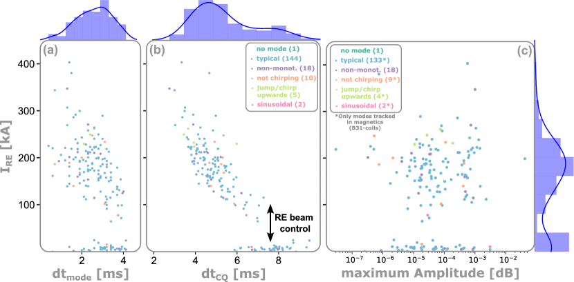
Figure 12: Runaway current $I_{\textnormal{RE}}$ plotted against the mode duration in (a), current quench duration in (b) and mode amplitude in (c). No effect of the mode amplitude on the RE beam current is observed in (c).

Most importantly, as shown in figure 12(c), we do not observe a decreased runaway current for increased mode amplitudes. The points seem to be more scattered, and there is no clear trend that one could identify between mode amplitude and runaway beam current. This shows that there appears to be little causal relation between the two in either direction. The REs are not expected to undergo resonant wave-particle interaction with MHD modes at the observed frequencies of a few hundred kHz. It also appears that the modes don’t have sufficient amplitude to perturb the field enough for transport to overcome RE generation.

7 Simulation analysis

While compressional Alfvén eigenmodes (CAEs) are used as a possible explanation for the observations at DIII-D [24, 25, 36, 37] the modes observed on ASDEX Upgrade appear in different frequency ranges. We therefore propose a different potential driving mechanism for the post-disruption modes, which are identified as global Alfvén eigenmodes (GAEs).

We performed ASTRA simulations [26] for the reference discharge #35618. These simulations provide local plasma parameters such as the $q$- or the electron and ion temperature profiles. Together with the equilibrium reconstruction [38, 39], the data was fed into LIGKA [40, 41] simulations. In figure 13 the temperature and density profiles for electrons and ions is provided as well as the safety factor (q) profile.

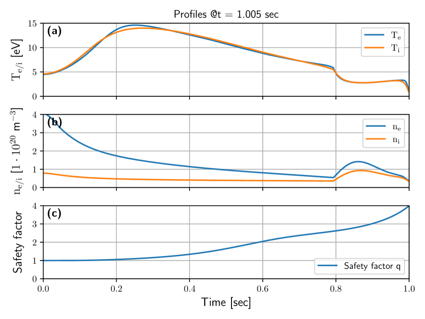
Figure 13: Excerpt of the plasma profiles used as input for the LIGKA simulations. The temperature (a) and density (b) profiles for electrons and ions as well as the q-profile (c) is provided.

LIGKA (LInear GyroKinetic shear Alfvén physics) is an eigenmode solver, which was used to calculate the post-disruption Alfvén continuum, shown in figure 14.

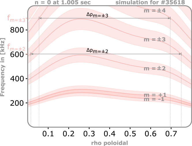
(a) LIGKA results for $t=1.005\ \textrm{s}$. The gray arrows show the potential radial extent of the $m=2$ and $m=3$ mode.

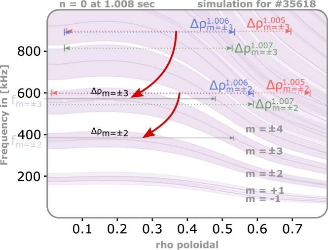
(b) LIGKA results for $t=1.008\ \textrm{s}$. The dashed lines ($\textnormal{f}_{m=\pm 2/3}^{time}$) represent the $m=2$ and $m=3$ maxima for $t=1.005,1.006\ \textnormal{and }1.007\ \textrm{s}$, respectively.

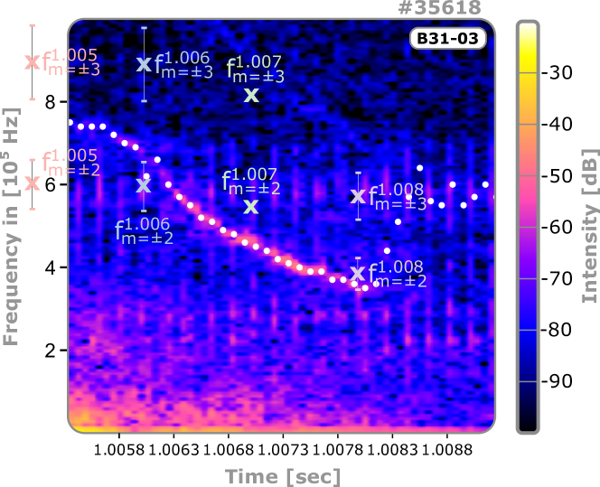
(c) Spectrogram for magnetic pick-up coil B31-03 with the frequency evolution from plots (a) – (e).

Figure 14: Results from LIGKA simulations for discharge #35618. The plots in (a) and (b) show the Alfvén continuum. GAEs can be exited above the maxima, thus their frequency (f) and potential radial extent ($\Delta\rho$) can be estimated. The expected frequency evolutions are compared to the experimental result in (c).

In (a) and (b) the results from LIGKA for a fixed toroidal mode number of $n=0$ are presented for different time points. This mode number was chosen based on the results of the mode number analysis (section 4). The plots show the coupled Alfvén continuum as solid lines. The shaded areas around the central lines show the results for a 20% in-/decrease in ion density. In addition, the first four poloidal mode numbers are labeled in the plot. The ASTRA simulations yield, that the electron temperature and $q$ profiles are highly peaked due to pre-injection application of strong central ECRH. Consequently, extrema are visible in the Alfvén continuum.

For typical experimental setups, this extremum is most likely a minimum in the Alfvén continuum [42, 43]. This is due to higher peaked plasma current profiles compared to density profiles for present day tokamaks [43]. Therefore, GAEs are expected just below the minima in the Alfvén continuum for typical scenarios [42, 43]. However, during disruptions – especially during ones mitigated via impurity injection – the plasma profiles vary significantly. This also affects the $q$-profile, the Alfvén velocity and continuum. Higher plasma densities towards the edge region can also lead to the formation of a maximum in the continuum, which is visible in the plots in figure 14(a) and (b). GAEs are expected to be present slightly above this maximum for these cases.

For this reason, we performed plasma response scans at these maxima (at the position of the gray arrows in figure 14(a)) in the LIGKA simulations. Hereby, excitations by an artificial test-antenna are mimicked and the plasma response to these waves is monitored. Strong reactions of the plasma to these waves hint towards potential modes excited by these waves. The results of the scans above the $m=2$ or $m=3$ maximum, are given in figure 15. Here the value of the eigenfunctions are plotted against the radial position and the lines represent the different mode numbers of the plasma response. The response is strongest for the mode number affiliated with the maxima of the Alfvén continuum scanned. Therefore, the strongest response is measured for $m=2$ and $m=3$ above the $m=2$ and $m=3$ maximum, respectively.

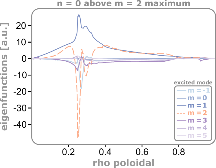
(a) LIGKA scans above $m=2$ maximum.

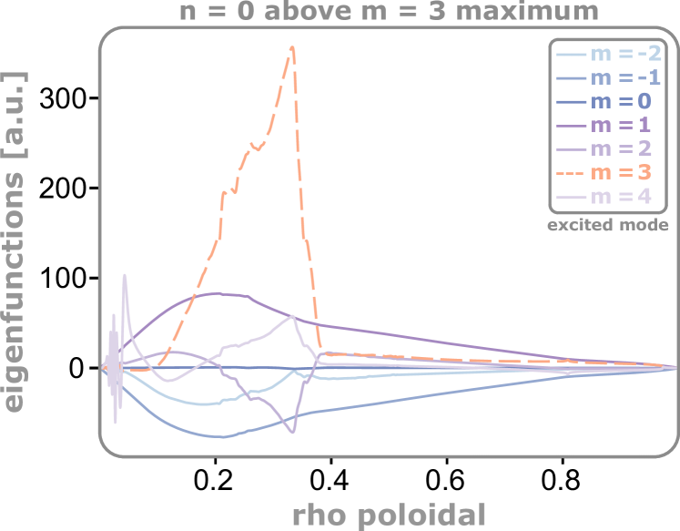
(b) LIGKA scans above $m=3$ maximum.

Figure 15: Plasma response scans in the LIGKA simulations. An artificial test-antenna is mimicked, launching waves into the plasma and monitoring the plasma response. The respective $m=2,3$ contributions are highlighted by the dashed lines.

As shown in figure 15, we are likely to excite modes (namely GAEs) above these maxima. We can now use this information and track the mode behaviour for different time points shown in figure 14. For $t=1.005\ \sec$ (figure 14(a)), we highlighted the modes with $m=2$ and $m=3$, which are in a similar frequency range as the mode observed for this discharge. The gray horizontal lines show the potential radial extent of excited modes. At the intersection with the continuum lines, continuum damping will occur, thus is very likely to set a limit to the radial extent. As the mode frequency will be close to the maxima of the peaked profiles, it is also possible to extract the frequency evolution from the plot. The frequencies, including the error bars from the 20% change in ion density, are plotted on top of the spectrogram for the magnetic pick-up coil B31-03 in figure 14(c). With time, the profiles evolve and the frequencies of the excited waves change, as indicated by the red arrows in figure 14(b). Following the maxima of the profiles, the mode frequency decreases as observed also in the experiment. At $t=1.008\ \sec$ (figure 14(b)) the peaked profiles flatten and the maxima vanish. With this, we also expect the mode to cease, matching the experimental observations displayed in the spectrogram 14(c). However, the frequency evolutions predicted by the simulation results do not quite match the experimental results. While the $m=2$ mode would match the observations well for later times, the starting frequency is slightly underestimated. However, matching the experiment with the ASTRA simulations for discharge #35618 had been challenging, thus future simulations might increase the precision of the frequency predictions. This first analysis of the CQ modes does not include investigations for possible mode driving mechanisms. Based on the also prominent $n=-4$ contribution of the mode number investigations, the mode might rotate in the ion diamagnetic direction with a mode frequency below the ion cyclotron resonances. Therefore, the modes might be driven by drift reversed trapped electrons or by non-linear excitation mechanisms, such as wave-wave coupling processes.

8 Summary

For safe operation of next step fusion reactors, the suppression of runaway electron beams is an essential task. Making use of intrinsically or externally driven Alfvénic activity during the current quench phase could be an actuator for runaway electron mitigation. In this paper, we show the results from a detailed study on the behaviour and statistics of modes in post-disruption plasmas in ASDEX Upgrade and explain their frequency change by gaps in the GAE continuum.

The modes appear exclusively during the current quench and typically sweep from higher to lower frequencies in a range around 800 kHz to 300 kHz for the first harmonic with their most likely frequency around 400 kHz. The modes are globally coherent, however, are composed of many different mode numbers, thus do not show a unique mode number. The most prominent toroidal mode numbers are $n=0$ and $n=-4$, where the negative sign indicates a propagation in the ion diamagnetic drift direction. The statistical analysis was performed on a database consisting of 180 disruptions aiming for runaway electron generation, which shows the presence of a mode in 179 cases.

The mode behaviour does not show strong correlations with global parameters, such as plasma current or magnetic field properties. Even though the mode length correlates with the subsequent runaway current, the mode amplitude does not. Moreover, the cause of this correlation might be the connection to the current quench duration, which sets the boundary conditions for the appearance of these modes. Modes were also observed in natural disruptions with no subsequent RE beam. The analysis of “multi-stage” disruptions revealed, that the modes appear exclusively after the last $\textnormal{I}_{\textnormal{p}}$ spike occurred, indicating that the conditions of the mode appearance is more complex as simple critical thresholds in the plasma current.

We performed dedicated ASTRA and LIGKA simulations to investigate the mode origin. We were able to reproduce a similar frequency evolution to our reference discharge #35618. First, an ASTRA simulation was performed to access local plasma parameters such as the safety factor and temperature profile. LIGKA simulations for a fixed toroidal mode number of $n=0$ revealed gaps in the GAE-continuum, where mode activity can be excited. Following the changes in the local plasma parameters over time, those gaps shift towards lower frequency, which can explain the sweeping behaviour of these modes. Moreover, the flattening of the Alfvén continuum profiles at $t=1.008$ sec will cause the mode to vanish, matching our experimental observations. Within the error bars, the absolute frequency is reasonably matched for a mode with an poloidal mode number of $m=\pm 2$. The mode driving mechanisms were not investigated during these studies, however, potential candidates could be drift reversed trapped electrons or non-linear excitation mechanisms, like wave-wave coupling.

We conclude, that the modes observed at ASDEX Upgrade and reported on in this paper do not have sufficient amplitude to have a significant impact on runaway electron dynamics in these ASDEX Upgrade scenarios. It remains to be seen, if modes in a different frequency range, and / or higher amplitudes can be achieved in ASDEX Upgrade runaway electron scenarios.

Appendix A Appendix

A.1 Correlation Matrix including 4 regions of interest

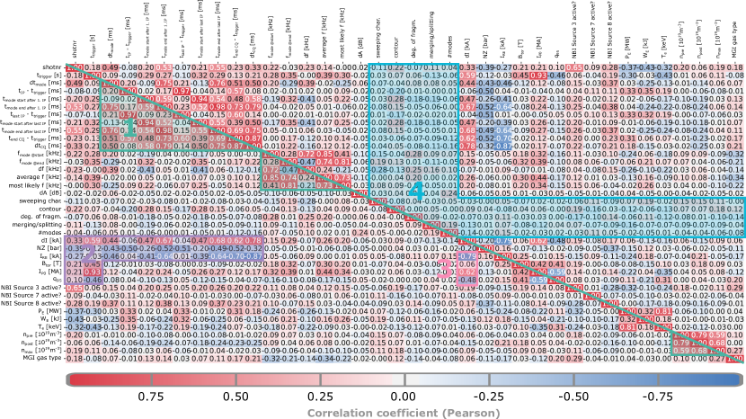
Figure 16: The correlation matrix with Pearson correlation coefficients.

Table 4: Excerpt of parameters inside the database.

PARAMETER DESCRIPTIONS
parameter [unit]	description
shotnr	ID of the discharge. The routine/setup might change between discharges.
$t_{\textnormal{trigger}}$ [s]	Time when the MGI valve was triggered. $t_{\textnormal{trigger}}=1.0$ s for 160/180 discharges.
$\textnormal{d}t_{\textnormal{mode}}$ [ms]	Duration of the mode given by the mode tracing tool (user selection of start and end points by hand).
$t_{\textnormal{IP}}-t_{\textnormal{trigger}}$ [ms]	Time point of the initial $\textnormal{I}_{\textnormal{p}}$ spike.
$t_{\textnormal{mode start after 1. IP}}$ [ms], $t_{\textnormal{mode end after 1. IP}}$ [ms]	Start & end time of the mode with respect to the initial $\textnormal{I}_{\textnormal{p}}$ spike
$t_{\textnormal{last IP}}-t_{\textnormal{trigger}}$ [ms]	Time point of the last $\textnormal{I}_{\textnormal{p}}$ spike for multi-stage disruptions.
$t_{\textnormal{mode start after last IP}}$ [ms], $t_{\textnormal{mode end after last IP}}$ [ms]	Start & end time of the mode with respect to the last $\textnormal{I}_{\textnormal{p}}$ spike
$t_{\textnormal{end CQ}}-t_{\textnormal{trigger}}$ [ms]	End time with respect to the trigger time.
$\textnormal{d}t_{\textnormal{CQ}}$ [ms]	Length of the CQ. Defined by the initial $\textnormal{I}_{\textnormal{p}}$ spike and when the temporal derivative approaches 0 again.
$f_{\textnormal{mode \@start}}$ [kHz]	Starting frequency of the mode.
$f_{\textnormal{mode \@end}}$ [kHz]	Frequency at the end of the mode.
d$f$ [kHz]	Change in frequency $f_{\textnormal{mode \@end}}-f_{\textnormal{mode \@start}}$
average $f$ [kHz]	Average mode frequency derived by the arithmetic mean.
most likely $f$ [kHz]	Most likely frequency of the mode (see section 6.1).
$A_{\textnormal{min}}$ [dB], $A_{\textnormal{max}}$ [dB]	Minimum/Maximum mode amplitude.
d$A$ [kHz]	Difference in mode amplitude $A_{\textnormal{max}}-A_{\textnormal{min}}$.
sweeping char.	Rating of the sweeping characteristic from typical (1) – sinusoidal (5) and no mode (0).
contour	Rating of the mode contour from narrow (1) – very cloud like (5) and no mode (0).
deg. of fragm.	Rating of the degree of fragmentation from not fragmented (1) – strongly fragmented (5) and no mode (0).
merging/splitting	Rating of the mode merging & splitting behaviour from not merging nor splitting (1) – splitting and merging (5) and no mode (0).
#modes	Number of prominent modes inside the CQ.
$I_{\textnormal{P0}}$ [MA]	Pre-disruption plasma current.
$I_{\textnormal{RE}}$ [kA]	Runaway current after the CQ.
d$I$ [kA]	Difference between the pre-disruption and runaway current.
NZ [bar]	Amount of MGI gas injected.
$B_{\textnormal{tor}}$ [T]	Toroidal magnetic field strength.
$q_{\textnormal{95}}$	Value of the safety factor at $\rho_{\textnormal{pol}}=0.95$.
NBI-source 3/7/8 active?	States whether the respective NBI source 3, 7 and 8 is active (0 = not active, 1 = active).
$P_{\textnormal{E}}$ [MW]	Average heating power by ECRH before the valve is triggered.
$W_{\textnormal{E}}$ [kJ]	Plasma stored energy.
$T_{\textnormal{e}}$ [keV]	Electron temperature measured by ECE-measurements.
$n_{\textnormal{pre}}$ [$10^{19}\leavevmode\nobreak\ \textnormal{m}^{-3}$]	Pre-disruption plasma density measured by $\textnormal{CO}_{2}$ interferometry (LOS: V-1).
$n_{\textnormal{post}}$ [$10^{19}\leavevmode\nobreak\ \textnormal{m}^{-3}$]	Post-disruption plasma density measured by $\textnormal{CO}_{2}$ interferometry (LOS: V-1).
$n_{\textnormal{max}}$ [$10^{19}\leavevmode\nobreak\ \textnormal{m}^{-3}$]	Maximum plasma density measured by $\textnormal{CO}_{2}$ interferometry (LOS: V-1).
MGI gas type	One of the following four gas types are used for the MGI: Ar, Ne, Kr or Xe with numbers 1–4 assigned.

A.2 Highlighted regions in the correlation matrix

Region 1 shows high (positive) correlation values, thus is one of the first regions drawing the attention onto it. It is attached to the principal diagonal, therefore it shows the correlation results for factors close to each other in the factor list. It depicts the three blocks of time-, frequency- and density-components. Let us pick the frequency block as an example. If we have a high starting frequency ($f_{\textnormal{mode @start}}$ [kHz]), the difference in frequency (d$f$ [kHz]) and also the average frequency (average $f$ [kHz]) is more likely to be high. As a result, their correlation value is close to +1. Similar internal connections also apply to the other blocks of region 1.

For region 2 this is not the case anymore. It is located far from the principal diagonal and connects the time block with global parameters such as the (runaway) current, toroidal magnetic field strength and $q_{95}$. Let us focus on the current measurements first. The mode lives inside the CQ as indicated in figure 4. For longer current quench and mode duration, lower subsequent currents are held by runaway electrons ($I_{\textnormal{RE}}$ [kA]) and a higher change in current (d$I$ [kA]) will be achieved (see figure 12). This results in high correlation values – positive for the change in current, negative for the runaway current. Another observation of this block is the anti-correlation between the amount of gas injected to trigger the disruption ($\textnormal{N}_{\textnormal{Z}}$ [bar]) and the start ($t_{\textnormal{IP}}-t_{\textnormal{trigger}}$ [ms]) and end ($t_{\textnormal{end CQ}}-t_{\textnormal{trigger}}$ [ms]) times of the current quench, respectively. The values for the safety factor $q_{95}$ are typically adjusted by varying the plasma current and toroidal magnetic field. As the pre-disruption plasma current is determined by the timing of the MGI, the trigger time shows correlations with $B_{\textnormal{tor}}$ and $q_{95}$. Thereby, earlier injections lead to lower plasma currents, hence higher safety factors.

In region 3 the correlation between the change in current (d$I$ [kA]) and respective runaway current ($I_{\textnormal{RE}}$ [kA]), pre-disruption current ($I_{\textnormal{P0}}$ [MA]) and q95, are shown. It is expected for d$I$ and $I_{\textnormal{RE}}$ to anti-correlate, as well as d$I$ and $I_{\textnormal{P0}}$ to correlate, as already indicated in the explanations for region 2. The correlation between $q_{95}$ and d$I$, can be linked to two different factors. First again $q_{95}$ and $I_{\textnormal{P0}}$ are connected as the plasma current is one of the factors determining $q$. Hence, lower plasma currents often result in higher safety factors and at the same time only allow reduced changes in plasma current. Additionally, it is observed for ASDEX Upgrade, that if $q_{95}<3$ no RE plateau is forming [44]. As no RE plateau is present for safety factors below three, the potential change in current is higher.

Region 4 shows the correlation values of the mode characteristics introduced in section 5. This region is of special interest, as high correlation results would point towards a connection between the mode behaviour and global parameters. However, we do not observe any significant correlations in this region! The higher values within this region, e.g. for the correlation of the change in frequency (d$f$ [kHz]) with the sweeping characteristic, can be explained due to the rating system. For this example the sweeping characteristic is granted a number between 1 (typical) to 5 (sinusoidal) (and 0 for no mode). Number 3 is assigned to the behaviour not chirping. The anti-correlation is caused by the typical sweeping behaviour having a larger change in frequency compared to the not chirping one. So by increasing the rating-number from 1 to 3 the change in frequency decreases. Similar effects of the rating system are observed for other characteristics.

A.3 Potential explanations for the loadings of each principal component in figure 11

1. The first underlying factor 1 groups mainly the end times of the modes with the current evolution, which was discussed for region 2 in section 6.2.1.

2. Here, the frequency properties of the modes are addressed. In section 6.1 a comparison between the average and most likely frequency is provided. Hereby, the end frequency of the mode has the most influence on the average and most likely frequency, respectively. Therefore, the loading for the start frequency is lower compared to the other loadings.

3. This factor illustrates the current ramp-up phase. When the MGI valve is triggered at later times, higher pre-disruption plasma currents and lower safety factors are present. This also affects the possible change in current d$I$.

4. Higher amounts of gas injected into the chamber will lead to earlier $\textnormal{I}_{\textnormal{p}}$ spike times and ultimately also the end time of the current quench reduces.

5. In this principal component, the frequency properties of the mode are addressed. The start frequency and change in frequency show the highest loadings. The change in frequency is calculated via both – start and end frequency – however, the variation of the start frequency is typically larger compared to the range of end frequencies. Smaller loadings for the sweeping behavior and degree of fragmentation and are also visible. A possible explanation for this is presented in the following, with discharge #35624 in figure 7(c) as an example. As the beginning of the mode does not show a continuous mode evolution, it was rated as ”strongly fragmented”. The starting frequency of the mode is around 680 kHz and the other part of the mode between 400 – 370 kHz. In case of reduced visibility of the mode in the spectrogram – due to a bad SNR or any physical reason – the traced mode would start at later times with a lower frequency. Accordingly, a decreased change in frequency and mode duration would be measured. In addition, without the first fragments of the mode being visible, this mode would not be considered as ”fragmented” anymore, hence, the degree of fragmentation would decrease, which could explain the loadings in this principal component. In-/excluding the first part of the mode for the discharge #36425 would not affected the MLF, as it is mainly determined by the end frequency of the mode at the flat tail. This matches the MLFs-loading close to zero.

6. The plasma density measurements at different times are connected via factor 6. For higher pre-disruption densities also a higher post-disruption and maximum density is expected.

7. Here, mainly the start times of the modes after the first and last $\textnormal{I}_{\textnormal{p}}$ spike are connected. As only five discharges within the database contain multiple $\textnormal{I}_{\textnormal{p}}$ spikes during incomplete disruptions (see figure 5), mostly the first $\textnormal{I}_{\textnormal{p}}$ spike is also the last $\textnormal{I}_{\textnormal{p}}$ spike at the same time. Therefore, the values match most of the time. Additionally, smaller loadings for the change in frequency and mode contour characteristic are contained. For this, two effects could explain these loadings: Firstly, the accuracy of the correct start time of the mode. For larger mode contour rating numbers – especially the ”extended” modes, it is increasingly difficult to pin down an exact start and end time of the mode. Therefore, the actual start of the mode might be sometimes earlier than determined by hand. A more detailed illustration of this is given in the thesis by P. Heinrich [30]. As the modes often chirp strongest at their start, the change in frequency is affected by this as well. On the other hand, extended modes were observed have a lower chirping rate on average compared to modes with a smaller spectral width.

8. Illustration of changes in the heating schemes over the course of the experimental campaign. In later discharges, the NBI source 3 with different heating schemes were used compared to the older discharges.

9. The safety factor is directly proportional to the strength of the toroidal magnetic field component, which is illustrated by the loadings for factor 9.

References

- [1] G. Pautasso et al. Nuclear Fusion, \hrefhttps://dx.doi.org/10.1088/0029-5515/55/3/03301555 (3):033015 (2015).
- [2] G. Pautasso et al. Plasma Physics and Controlled Fusion, \hrefhttps://doi.org/10.1088/0741-3335/59/1/01404659 (1):014046 (2016).
- [3] G. Pautasso et al. Nuclear Fusion, \hrefhttps://doi.org/10.1088/1741-4326/ab956360 (8):086011 (2020).
- [4] S. Jachmich et al. Nuclear Fusion, 62 (026012) (2022).
- [5] U. Sheikh et al. Nuclear Fusion, 61 (12):126043 (2021).
- [6] M. Lehnen et al. IAEA, London, United Kingdom (2023).
- [7] T. E. Gebhart et al. Nuclear Fusion (2021).
- [8] S. Jachmich et al. 2nd IAEA TM on Plasma Disruptions and their Mitigation, ITER Headquarters (2022).
- [9] E. Nardon et al. Nuclear Fusion (2021).
- [10] O. Vallhagen et al. Journal of Plasma Physics, \hrefhttps://doi.org/10.1017/S002237782300046689 (3):905890306 (2023).
- [11] I. Pusztai et al. Journal of Plasma Physics, \hrefhttps://doi.org/10.1017/S002237782300019389 (2):905890204 (2023).
- [12] A. H. Boozer. Nuclear Fusion, \hrefhttps://doi.org/10.1088/1741-4326/aa635557 (5):056018 (2017).
- [13] O. Vallhagen et al. Nuclear Fusion, \hrefhttps://dx.doi.org/10.1088/1741-4326/ac667e62 (11):112004 (2022).
- [14] B. N. Breizman et al. Nuclear Fusion, \hrefhttps://doi.org/10.1088/1741-4326/ab182259 (8):083001 (2019).
- [15] M. Rosenbluth et al. Nuclear Fusion, \hrefhttps://doi.org/10.1088/0029-5515/37/10/i0337 (10):1355 (1997).
- [16] L. Hesslow et al. Nuclear Fusion, \hrefhttps://dx.doi.org/10.1088/1741-4326/ab26c259 (8):084004 (2019).
- [17] G. F. Matthews et al. Physica Scripta, \hrefhttps://doi.org/10.1088/0031-8949/t167/1/014070T167:014070 (2016).
- [18] C. Paz-Soldan et al. Nuclear Fusion, \hrefhttps://dx.doi.org/10.1088/1741-4326/ac2a6961 (11):116058 (2021).
- [19] C. Reux et al. Plasma Physics and Controlled Fusion, \hrefhttps://dx.doi.org/10.1088/1361-6587/ac48bc64 (3):034002 (2022).
- [20] U. A. Sheikh et al. Plasma Physics and Controlled Fusion (2024).
- [21] P. Svensson et al. Journal of Plasma Physics, 87 (2):905870207 (2021).
- [22] A. Lier et al. Nuclear Fusion, 61 (086003) (2021).
- [23] A. Lier et al. Nuclear Fusion, \hrefhttps://dx.doi.org/10.1088/1741-4326/acc4de63 (5):056018 (2023).
- [24] A. Lvovskiy et al. Plasma Physics and Controlled Fusion, \hrefhttps://doi.org/10.1088/1361-6587/aae95a60 (12):124003 (2018).
- [25] A. Lvovskiy et al. Nuclear Fusion, 63 (046011) (2023).
- [26] O. Linder et al. Nuclear Fusion, \hrefhttps://doi.org/10.1088/1741-4326/ab9dcf60 (9):096031 (2020).
- [27] M. Schittenhelm et al. Nuclear Fusion, \hrefhttps://dx.doi.org/10.1088/0029-5515/37/9/I0637 (9):1255 (1997).
- [28] F. Mink et al. Plasma Physics and Controlled Fusion, \hrefhttps://dx.doi.org/10.1088/0741-3335/58/12/12501358 (12):125013 (2016).
- [29] L. Horváth et al. Nuclear Fusion, \hrefhttps://dx.doi.org/10.1088/0029-5515/56/11/11200356 (11):112003 (2016).
- [30] P. Heinrich. Investigations of Alfvénic activity during the current quench in ASDEX-Upgrade. Master’s thesis, Max-Planck-Institut für Plasma Physik, Garching (2021). http://hdl.handle.net/21.11116/0000-0008-ED5A-9.
- [31] A. Magyarkuti. Budapest University of Technology and Economics, Scientific Student Conference (TDK), Budapest University of Technology and Economics, Budapest, Hungary (2009).
- [32] T. Hender et al. Nuclear Fusion, \hrefhttps://doi.org/10.1088/0029-5515/47/6/S0347 (6):S128 (2007).
- [33] L. Horváth et al. Plasma Physics and Controlled Fusion, \hrefhttps://dx.doi.org/10.1088/0741-3335/57/12/12500557 (12):125005 (2015).
- [34] A. G. Yong et al. Tutorials in quantitative methods for psychology, 9 (2):79 (2013).
- [35] Factoranalyzer documentation. https://factor-analyzer.readthedocs.io/en/latest/index.html. Accessed: 2020-12-15.
- [36] C. Liu et al. Nuclear Fusion, \hrefhttps://doi.org/10.1088/1741-4326/abcfcf61 (3):036011 (2021).
- [37] C. Liu et al. Phys. Rev. Lett., 131 (8):085102 (2023).
- [38] P. J. Mc Carthy. Physics of Plasmas, \hrefhttps://doi.org/10.1063/1.8736306 (9):3554 (1999).
- [39] M. Dunne et al. Nuclear Fusion, \hrefhttps://doi.org/10.1088/0029-5515/52/12/12301452 (12):123014 (2012).
- [40] P. W. Lauber. Linear Gyrokinetic Description of Fast Particle Effects on the MHD Stability in Tokamaks. Dissertation, Technische Universität München, München (2003).
- [41] P. W. Lauber et al. Journal of Computational Physics, \hrefhttp://www.sciencedirect.com/science/article/pii/S0021999107001660226 (1):447 (2007).
- [42] W. W. Heidbrink. Physics of Plasmas, \hrefhttps://doi.org/10.1063/1.283823915 (5):055501 (2008).
- [43] K. Appert et al. Plasma Physics, 24 (9):1147 (1982).
- [44] G. Papp et al. 46th EPS Conference on Plasma Physics, Milan, Italy (2019).