Cascaded Scaling Classifier: class incremental learning with probability scaling

Abstract

Humans are capable of acquiring new knowledge and transferring learned knowledge into different domains, incurring a small forgetting. The same ability, called Continual Learning, is challenging to achieve when operating with neural networks due to the forgetting affecting past learned tasks when learning new ones. This forgetting can be mitigated by replaying stored samples from past tasks, but a large memory size may be needed for long sequences of tasks; moreover, this could lead to overfitting on saved samples. In this paper, we propose a novel regularisation approach and a novel incremental classifier called, respectively, Margin Dampening and Cascaded Scaling Classifier. The first combines a soft constraint and a knowledge distillation approach to preserve past learned knowledge while allowing the model to learn new patterns effectively. The latter is a gated incremental classifier, helping the model modify past predictions without directly interfering with them. This is achieved by modifying the output of the model with auxiliary scaling functions. We empirically show that our approach performs well on multiple benchmarks against well-established baselines, and we also study each component of our proposal and how the combinations of such components affect the final results.

1 Introduction

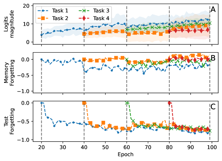
Figure 1: We train a ResNet-20 model with a simple rehearsal approach and a memory size of 500, on CIFAR10 divided into 5 tasks. A) Magnitude of ground truth logits on the replay samples; B) Forgetting on the replay samples; C) Forgetting on test scores for each past task.

Building an agent capable of continuously learning over time from a stream of tasks remains a fundamental challenge. This ability is called Continual Learning (CL), a key property enabling autonomous real-world agents. Traditional machine learning models often struggle when faced with sequential and non-stationary data due to Catastrophic Forgetting (CF), which often leads to a drastic performance decrease due to the overwriting of past learned knowledge while learning new one (Parisi et al., 2019). The desired balance between remembering past learned patterns and correctly acquiring new knowledge is often called stability-plasticity trade-off (Wang et al., 2023).

The most straightforward way to mitigate CF is by using rehearsal-based approaches, which store and replay a small subset of previous task samples, but how such samples must be saved and retrieved is an open question. It is challenging to keep generally discriminative past samples because of overfitting that arises from replaying them (Verwimp et al., 2021; Prabhu et al., 2020; Buzzega et al., 2020; Bonicelli et al., 2022). In such scenarios, additional complexity comes from the intrinsically unbalanced nature of the training procedure, in which newer patterns have more samples than the ones in the memory. Consider the example shown in Fig. 1. Overfitting on rehearsal samples leads to a growth of their ground truth logits during the whole training procedure. At the same time, the forgetting on the test samples is higher than the one achieved on rehearsal samples. Intuitively, these two quantities should be similar, showing that this approach is not fighting the CF but only overfitting patterns present in the external memory. This is evident by looking at scores achieved for tasks 3 and 4, in which forgetting on replay samples is nearly zero across all the training, and often becomes positive, while the accuracy on the corresponding test sets rapidly decreases. Despite such limitations, using past samples as training ones is one of the most used approaches to fight the CF.

Usually, a rehearsal approach is coupled with a regularisation strategy, in which past samples are used to calculate a regularisation term added to the training loss to alleviate CF further. In such scenarios, the true nature of the forgetting still needs to be understood. Some works claim it could arise from the classifier (Ahn et al., 2021; Wu et al., 2019; Zhao et al., 2020; Li & Hoiem, 2017), and most of the time the output of the model is directly regularised to mitigate this. The regularisation is usually carried out by forcing the classifier to produce the same output distribution as in the past only for rehearsal samples. This combination creates two losses that are in contrast, because training on past samples leads to overfitting while regularising on them forces the model to produce the same output as in the past. Such approaches usually require a careful selection of the hyperparameters to balance these two aspects. This behaviour is shown in Appendix A.

Motivated by these observations, we propose a novel CL approach composed of a regularisation term and a novel incremental classifier head. The former modifies the probabilities of previous classes up to a certain margin which satisfies a given constraint while, at the same time, regularising all the classes using a Knowledge Distillation (KD) approach calculated over the whole output of the model. The latter is a hybrid classifier composed of smaller task-wise classifiers, which are scaled and combined to produce the final output distribution. The combination of such components is capable of correctly regularising past learned knowledge without training on past samples, avoiding overfitting of such samples. At the same time, current patterns are correctly learned without interfering with past learned ones. To demonstrate the effectiveness of our proposals, we conduct comprehensive experiments on multiple CL benchmarks, as well as in-depth exploratory experiments to analyse the effectiveness of core design choices of both the regularisation approach, called Margin Dampening (MD), as well as the classification head, which we call Cascaded Scaling Classifier (CSC). For space reasons, an analysis of related works can be found in Appendix B.

2 Continual Learning definition

In a Class Incremental Learning (CIL) scenario, a generic model $f(\cdot)$ is trained on a sequence of classification tasks $\mathbf{T}=\{\mathcal{T}_{i}\}$, with $i=1,\dots,T$, having complete access only to the current training task $t$, with the additional possibility of storing a subset of past tasks’ samples. A generic task consists of a tuple $\mathcal{T}_{i}=(\mathcal{D}^{i},\mathrm{Y}^{t})$, where $\mathcal{D}^{i}=\{(x_{i},y_{i})\}$ is the dataset containing the samples and $y_{i}\in\mathrm{Y}^{t}$ is the label space of the task $t$, such that $\bigcap_{t=1,\dots,\text{T}}\mathrm{Y}^{t}=\varnothing$; no other assumptions are made on the labels’ space except that $\lvert\mathrm{Y}^{t}\rvert\geq 2$ for each task $t$. Moreover, by definition, in a CIL scenario task identities are present only during training but not in the inference phase. This key difference makes CIL harder than another CL scenario called Task Incremental Learning (TIL), because having access to the task identities during inference allows for better separation between tasks, drastically reducing CF effects. For this reason, TIL can be easily solved using an architectural approach (Golkar et al., 2019; Wortsman et al., 2020) or even employing a regularisation approach without additional external memory (Pomponi et al., 2022).

Formally, we aim to fit a model $f:\mathcal{X}\rightarrow\mathcal{Y}^{\text{T}}$, where $\mathcal{Y}^{\text{T}}=\bigcup_{t=1,\dots,\text{T}}\mathrm{Y}^{t}$, which minimises the expected risk:

$$f^{*}=\operatornamewithlimits{argmin}\limits_{f}\underset{(x,y)\sim\bigcup_{i=1}^{\text{T}}\mathcal{D}^{i}}{\mathbb{E}}\,\mathcal{L}(f(x),y)$$ (1)

where $\mathcal{L}$ stands for the loss (e.g. cross-entropy loss) of correctly classifying sample $x$ having label $y$ using the model $f$. A generic model $f$ used in a CL scenario can be further decomposed into a backbone $b(\cdot)$ and a classification head $h^{t}(\cdot)$, which can be conditioned to the task $t$, such that $f^{t}(x)=h^{t}(b(x))$. No assumptions are made about the model, but usually, in a CIL scenario the backbone is given and its structure is fixed, while the output of the model is adapted each time a new task is retrieved. This is done by modifying the output of the classifier such that its output size is expanded to match the total number of classes, including the new ones; we also operate in this setting.

The goal of the minimisation process is to find the optimal model capable of minimising the loss over all the tasks. However, when training on a given task $t$ we cannot access the whole past tasks $t^{\prime}<t$, making this minimisation infeasible. To overcome this constraint while training on a task $t>1$ we can use a regularisation function $\mathcal{R}$, an external memory $\mathcal{M}$ containing a small portion of past samples, or combine these two approaches, as such:

$$f^{*}=\operatornamewithlimits{argmin}\limits_{f}\underset{(x,y)\sim\mathcal{D}^{t}\cup\mathcal{M}}{\mathbb{E}}\,\mathcal{L}(f(x),y)+\mathcal{R}(x,y)$$ (2)

A well-crafted CL approach term prevents the model from forgetting past learned knowledge while leaving room for learning new patterns from the current task. This is an important trade-off which must be considered when operating in a CL scenario, and it is called stability-plasticity trade-off (Wang et al., 2023).

3 Proposed training schema

Our proposal is composed of a custom head classifier $h^{t}(\cdot)$ called Cascaded Scaling Classifier (CSC), and a rehearsal regularisation approach, named Margin Dampening (MD). Combining these two components produces a method capable of achieving a better stability-plasticity trade-off, leading to better results.

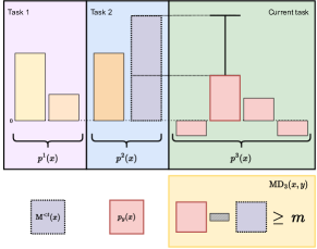
(a) Margin Dampening

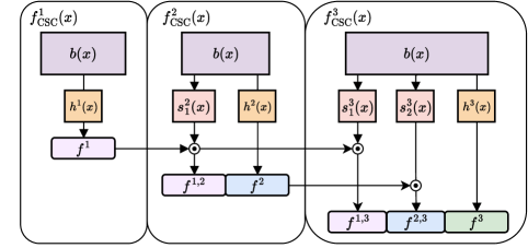
(b) Cascaded Scaling Classifier

Figure 2: On the left we show the probability dampening schema (MD, Section 3.1), in which past probabilities are decreased up to a certain margin, resulting in a regularisation approach based on a soft constraint. On the right, we visualise the cascaded procedure (CSC, Section 3.2), which combines task-wise outputs to build the final prediction. Better viewed in colours.

3.1 Margin Dampening (MD) regularisation

For a given tuple $(x,y)\in\mathcal{T}_{t}$, with $t>1$, the core idea of our regularisation schema is to decrease past probabilities while training only the output logits related to the current task, by forcing the maximum probability from past tasks to be lower than the ground truth probability, plus a safety margin. Denoting by $p(x)\in\mathbb{R}^{\lvert\mathcal{Y}^{t}\rvert}$ the vector containing the global probabilities for all classes seen up to the current task $t$, we calculate the maximum past probability as $\text{M}^{<t}(x)=\max_{c\in\mathcal{Y}^{t-1}}{p_{c}(x)}$. Using such value along with the ground truth probability $p_{y}(x)$, we want the minimization procedure to satisfy the following inequality:

$$p_{y}(x)-\text{M}^{<t}(x)\geq m$$ (3)

where $m$ is the margin value which controls the safe distance between the two quantities. The constraint translates into the Margin Dampening (MD) loss, defined as:

$$\text{MD}_{t}(x,y)=\max\left(0,\,\text{M}^{<t}(x)-p_{y}(x)+m\right)\\$$ (4)

which is summed to the cross-entropy loss calculated only over the classes belonging to the current task $t$, $p^{t}(x)\in\mathbb{R}^{\lvert\mathrm{Y}^{t}\rvert}$. The final loss while training on a task $t>1$ is:

$$\mathcal{L}_{t}(x,y)=\lambda\text{MD}_{t}(x,y)-\log\,p^{t}_{y}(x)$$ (5)

with $\lambda$ being a scaling value to balance the two terms, controlling the stability-plasticity trade-off. This loss works in a bidirectional manner: at the same time, the correct probability grows due to the minimisation of the cross-entropy loss calculated only over current classes, without interfering with past classes, while past probabilities are pushed down up to a certain point which is defined by the margin. Past this point, the regularisation loss becomes zero, creating a smoother and easier-to-optimise loss function. The proposed regularisation approach can be visually inspected in Figure 2a.

In addition to the training loss just exposed, which is calculated only over samples from the current task, we use past samples to calculate a KD regularisation term which enforces the stability of the model. In literature, the KD is divided, usually, into General KD (Zhao et al., 2020), which aggregates together logits belonging to the classes from all the previous tasks, and Task-wise approaches (Ahn et al., 2021), which treat classes within each task separately. Based on the intuition that newly added classes are randomly produced since the corresponding classifiers are randomly initialised, resulting in logits which are lower than the already trained ones, we propose a third way. Our regularisation term regularises the output of the model as a whole, without taking into account task boundaries. By doing so, we remove the necessity of training on past samples along with the ones from the current task, preventing the rise of overfitting of such samples.

To do that, we store a subset of past samples in an external memory $\mathcal{M}$ containing a fixed number of samples during the whole training, which is adapted by removing random portions of past samples when new ones must be stored. The samples are drawn in a class-balanced way and are used to regularise the output of the model as $\mathcal{R}(x)=\text{KL}(p(x)\,||\,\overline{p}(x))$, where $x\sim\mathcal{M}$, $\overline{p}(x)\in\mathbb{R}^{\lvert\mathcal{Y}^{t}\rvert}$, and KL is the Kullback-Leibler divergence. The latter can be seen as a teacher model, which has the same output as the model at the beginning of task $t$ before starting the training process, but after adapting the classification layer to match the total number of classes.

Selection of the margin: regarding the choice of the margin, we rely on the observation that a CIL scenario is defined in such a way that the number of classes grows with the number of tasks, which implies that the maximum probability obtainable decreases after each task. Following this intuition, the margin $m$ in Eq (4) must be scaled accordingly. To do that, we use a margin value which is based on how many classes have been encountered up to the current task $t$: $m^{t}=\frac{1}{\lvert\mathcal{Y}^{t}\rvert-1}$. By doing so, we avoid manually selecting the margin, which could result in either a disruptive or a negligible MD loss when not properly done. Not only does the margin value adapt while training, but it also allows the model to self-adapt based on the complexity of the training, removing the necessity to tune an additional hyperparameter.

Final loss: for a given tuple $(x,y)\in\mathcal{D}^{t}$ coming from the current task $t$, the final loss we propose is the following:

$$\mathcal{L}^{\text{MD}}_{t}(x,y,x_{m})=\left\{\begin{aligned} \quad&\begin{aligned} &\displaystyle\mathcal{L}_{t}(x,y)+\mathcal{R}(x_{m})\end{aligned}&\text{if }t>1\\ &-\log\,p_{y}(x)\quad&t=1\end{aligned}\right.$$

in which $x_{m}\sim\mathcal{M}$ and $\lvert x_{r}\rvert=\lvert x\rvert$, drawn in a class-balanced way.

3.2 Cascaded Scaling Classifier (CSC)

As opposed to standard heads used in literature, our approach is an ensemble of small task-wise heads, which are scaled and combined to produce the final output of the model. In this sense, our approach is a hybrid between a multi-head approach usually employed in TIL scenarios, and the single incremental one, which is the standard one used in the literature when dealing with CIL scenarios.

When a new task $t>1$ is retrieved, we not only add the corresponding task-wise head $h^{t}(b(x))\in\mathbb{R}^{\lvert\mathrm{Y}^{t}\rvert}$ into the classifier module, but also a set of scaling functions as $S^{t}(x)=\{s^{t}_{i}(x)\in\mathbb{R}^{\lvert\mathrm{Y}^{i}\rvert}\}$ for $i=1,\dots,t-1$. These additional modules are composed of a linear layer $g(\cdot)$, followed by a scaled Sigmoid such that $s^{t}_{i}(x)=\text{Sigmoid}(\gamma\cdot g(b(x))+\beta)$, in which we set $\gamma=1$ and $\beta=10$. Scaling the logits simplifies the regularisation of past classes without interfering directly with past heads. Mathematically, given the training task $t$ and a past task $i<t$, the output associated to $i$ is calculated as:

$$f^{i,t}(x)=f^{i}(x)\cdot\prod_{j=i+1}^{t}s^{j}_{i}(x)$$ (6)

with $f^{t,t}(x)=f^{t}(x)$. The final output of the model is produced by concatenating all such vectors:

$$f^{t}_{\text{CSC}}(x)=[f^{1,t}(x),f^{2,t}(x),\dots,f^{t}(x)]\in\mathbb{R}^{\rvert\mathcal{Y}^{t}\lvert}$$ (7)

where $t$ is the last task seen during the training procedure, which is fixed during the inference. Our final proposal is the combination of the just proposed head classifier, which can be visually inspected in Figure 2b, and the Margin Dampening regularisation proposed in Section 3.1.

4 Experimental Analysis

C10-5

C100-10

TyM-10

Naive

${18.62}_{\scaleto{\pm 0.1}{3pt}}{\scaleto{|\raisebox{0.8pt}{-}96.25_{\scaleto{\pm 1.0}{3pt}}}{8pt}}$

${8.0}_{\scaleto{\pm 0.3}{3pt}}{\scaleto{|\raisebox{0.8pt}{-}82.4_{\scaleto{\pm 0.1}{3pt}}}{8pt}}$

${6.2}_{\scaleto{\pm 0.5}{3pt}}{\scaleto{|\raisebox{0.8pt}{-}59.3_{\scaleto{\pm 1.5}{3pt}}}{8pt}}$

Cumulative

${86.8}_{\scaleto{\pm 0.5}{3pt}}{\scaleto{|\raisebox{0.8pt}{-}2.7_{\scaleto{\pm 1.1}{3pt}}}{8pt}}$

${61.4}_{\scaleto{\pm 0.4}{3pt}}{\scaleto{|\raisebox{0.8pt}{-}3.4_{\scaleto{\pm 0.4}{3pt}}}{8pt}}$

${30.0}_{\scaleto{\pm 0.7}{3pt}}{\scaleto{|\raisebox{0.8pt}{-}4.6_{\scaleto{\pm 0.5}{3pt}}}{8pt}}$

Memory Size

200

500

1K

2K

200

500

1K

2K

200

500

1K

2K

5K

Replay

${38.8}_{\scaleto{\pm 3.3}{3pt}}{\scaleto{|\raisebox{0.8pt}{-}69.4_{\scaleto{\pm 5.0}{3pt}}}{8pt}}$

${50.2}_{\scaleto{\pm 3.6}{3pt}}{\scaleto{|\raisebox{0.8pt}{-}53.6_{\scaleto{\pm 5.1}{3pt}}}{8pt}}$

${61.1}_{\scaleto{\pm 2.3}{3pt}}{\scaleto{|\raisebox{0.8pt}{-}38.8_{\scaleto{\pm 4.3}{3pt}}}{8pt}}$

${61.1}_{\scaleto{\pm 2.3}{3pt}}{\scaleto{|\raisebox{0.8pt}{-}31.0_{\scaleto{\pm 4.0}{3pt}}}{8pt}}$

${12.6}_{\scaleto{\pm 0.5}{3pt}}{\scaleto{|\raisebox{0.8pt}{-}74.0_{\scaleto{\pm 1.2}{3pt}}}{8pt}}$

${17.6}_{\scaleto{\pm 0.4}{3pt}}{\scaleto{|\raisebox{0.8pt}{-}66.6_{\scaleto{\pm 1.8}{3pt}}}{8pt}}$

${25.8}_{\scaleto{\pm 0.7}{3pt}}{\scaleto{|\raisebox{0.8pt}{-}56.1_{\scaleto{\pm 1.6}{3pt}}}{8pt}}$

${32.6}_{\scaleto{\pm 1.2}{3pt}}{\scaleto{|\raisebox{0.8pt}{-}46.1_{\scaleto{\pm 0.5}{3pt}}}{8pt}}$

${6.2}_{\scaleto{\pm 0.3}{3pt}}{\scaleto{|\raisebox{0.8pt}{-}55.5_{\scaleto{\pm 0.8}{3pt}}}{8pt}}$

${6.4}_{\scaleto{\pm 0.0}{3pt}}{\scaleto{|\raisebox{0.8pt}{-}51.9_{\scaleto{\pm 0.9}{3pt}}}{8pt}}$

${7.0}_{\scaleto{\pm 0.2}{3pt}}{\scaleto{|\raisebox{0.8pt}{-}50.4_{\scaleto{\pm 1.1}{3pt}}}{8pt}}$

${8.2}_{\scaleto{\pm 0.4}{3pt}}{\scaleto{|\raisebox{0.8pt}{-}46.8_{\scaleto{\pm 0.4}{3pt}}}{8pt}}$

${12.2}_{\scaleto{\pm 0.2}{3pt}}{\scaleto{|\raisebox{0.8pt}{-}38.2_{\scaleto{\pm 1.2}{3pt}}}{8pt}}$

GEM (Lopez-Paz & Ranzato, 2017)

${18.8}_{\scaleto{\pm 0.1}{3pt}}{\scaleto{|\raisebox{0.8pt}{-}88.9_{\scaleto{\pm 5.2}{3pt}}}{8pt}}$

${20.8}_{\scaleto{\pm 0.2}{3pt}}{\scaleto{|\raisebox{0.8pt}{-}89.7_{\scaleto{\pm 2.7}{3pt}}}{8pt}}$

${21.8}_{\scaleto{\pm 2.7}{3pt}}{\scaleto{|\raisebox{0.8pt}{-}82.2_{\scaleto{\pm 7.0}{3pt}}}{8pt}}$

${22.3}_{\scaleto{\pm 1.9}{3pt}}{\scaleto{|\raisebox{0.8pt}{-}82.9_{\scaleto{\pm 7.1}{3pt}}}{8pt}}$

${17.6}_{\scaleto{\pm 1.1}{3pt}}{\scaleto{|\raisebox{0.8pt}{-}68.1_{\scaleto{\pm 1.6}{3pt}}}{8pt}}$

${18.4}_{\scaleto{\pm 2.4}{3pt}}{\scaleto{|\raisebox{0.8pt}{-}59.1_{\scaleto{\pm 5.6}{3pt}}}{8pt}}$

${19.1}_{\scaleto{\pm 1.7}{3pt}}{\scaleto{|\raisebox{0.8pt}{-}54.3_{\scaleto{\pm 3.9}{3pt}}}{8pt}}$

–

${6.6}_{\scaleto{\pm 0.4}{3pt}}{\scaleto{|\raisebox{0.8pt}{-}53.4_{\scaleto{\pm 0.4}{3pt}}}{8pt}}$

${8.1}_{\scaleto{\pm 0.9}{3pt}}{\scaleto{|\raisebox{0.8pt}{-}46.7_{\scaleto{\pm 0.6}{3pt}}}{8pt}}$

${11.2}_{\scaleto{\pm 0.4}{3pt}}{\scaleto{|\raisebox{0.8pt}{-}41.1_{\scaleto{\pm 1.9}{3pt}}}{8pt}}$

–

–

DER (Buzzega et al., 2020)

${43.1}_{\scaleto{\pm 4.2}{3pt}}{\scaleto{|\raisebox{0.8pt}{-}64.4_{\scaleto{\pm 6.3}{3pt}}}{8pt}}$

${55.1}_{\scaleto{\pm 3.5}{3pt}}{\scaleto{|\raisebox{0.8pt}{-}48.4_{\scaleto{\pm 5.3}{3pt}}}{8pt}}$

${63.7}_{\scaleto{\pm 3.5}{3pt}}{\scaleto{|\raisebox{0.8pt}{-}36.4_{\scaleto{\pm 5.7}{3pt}}}{8pt}}$

${70.4}_{\scaleto{\pm 1.6}{3pt}}{\scaleto{|\raisebox{0.8pt}{-}26.1_{\scaleto{\pm 3.2}{3pt}}}{8pt}}$

${12.7}_{\scaleto{\pm 0.7}{3pt}}{\scaleto{|\raisebox{0.8pt}{-}74.7_{\scaleto{\pm 1.1}{3pt}}}{8pt}}$

${19.8}_{\scaleto{\pm 0.6}{3pt}}{\scaleto{|\raisebox{0.8pt}{-}64.7_{\scaleto{\pm 0.8}{3pt}}}{8pt}}$

${27.4}_{\scaleto{\pm 0.6}{3pt}}{\scaleto{|\raisebox{0.8pt}{-}54.9_{\scaleto{\pm 1.1}{3pt}}}{8pt}}$

${36.4}_{\scaleto{\pm 0.3}{3pt}}{\scaleto{|\raisebox{0.8pt}{-}43.2_{\scaleto{\pm 0.8}{3pt}}}{8pt}}$

${5.7}_{\scaleto{\pm 0.1}{3pt}}{\scaleto{|\raisebox{0.8pt}{-}55.7_{\scaleto{\pm 0.4}{3pt}}}{8pt}}$

${5.8}_{\scaleto{\pm 0.2}{3pt}}{\scaleto{|\raisebox{0.8pt}{-}54.4_{\scaleto{\pm 0.3}{3pt}}}{8pt}}$

${6.6}_{\scaleto{\pm 0.1}{3pt}}{\scaleto{|\raisebox{0.8pt}{-}51.7_{\scaleto{\pm 0.8}{3pt}}}{8pt}}$

${8.9}_{\scaleto{\pm 0.9}{3pt}}{\scaleto{|\raisebox{0.8pt}{-}51.5_{\scaleto{\pm 2.0}{3pt}}}{8pt}}$

${11.2}_{\scaleto{\pm 0.9}{3pt}}{\scaleto{|\raisebox{0.8pt}{-}49.2_{\scaleto{\pm 1.5}{3pt}}}{8pt}}$

GDUMB (Prabhu et al., 2020)

${24.5}_{\scaleto{\pm 1.0}{3pt}}{\scaleto{|\raisebox{0.8pt}{-}24.2_{\scaleto{\pm 5.2}{3pt}}}{8pt}}$

${31.1}_{\scaleto{\pm 1.6}{3pt}}{\scaleto{|\raisebox{0.8pt}{-}23.5_{\scaleto{\pm 7.3}{3pt}}}{8pt}}$

${36.8}_{\scaleto{\pm 1.9}{3pt}}{\scaleto{|\raisebox{0.8pt}{-}26.2_{\scaleto{\pm 8.2}{3pt}}}{8pt}}$

${45.2}_{\scaleto{\pm 1.6}{3pt}}{\scaleto{|\raisebox{0.8pt}{-}25.0_{\scaleto{\pm 3.1}{3pt}}}{8pt}}$

${3.6}_{\scaleto{\pm 0.4}{3pt}}{\scaleto{|\raisebox{0.8pt}{-}47.8_{\scaleto{\pm 6.4}{3pt}}}{8pt}}$

${6.7}_{\scaleto{\pm 0.2}{3pt}}{\scaleto{|\raisebox{0.8pt}{-}28.6_{\scaleto{\pm 2.0}{3pt}}}{8pt}}$

${9.5}_{\scaleto{\pm 0.4}{3pt}}{\scaleto{|\raisebox{0.8pt}{-}14.7_{\scaleto{\pm 0.7}{3pt}}}{8pt}}$

${14.1}_{\scaleto{\pm 0.4}{3pt}}{\scaleto{|\raisebox{0.8pt}{-}17.4_{\scaleto{\pm 2.0}{3pt}}}{8pt}}$

${0.9}_{\scaleto{\pm 0.1}{3pt}}{\scaleto{|\raisebox{0.8pt}{-}2.9_{\scaleto{\pm 0.3}{3pt}}}{8pt}}$

${2.0}_{\scaleto{\pm 0.1}{3pt}}{\scaleto{|\raisebox{0.8pt}{-}4.7_{\scaleto{\pm 1.9}{3pt}}}{8pt}}$

${3.2}_{\scaleto{\pm 0.2}{3pt}}{\scaleto{|\raisebox{0.8pt}{-}6.8_{\scaleto{\pm 1.1}{3pt}}}{8pt}}$

${5.1}_{\scaleto{\pm 0.3}{3pt}}{\scaleto{|\raisebox{0.8pt}{-}9.0_{\scaleto{\pm 0.8}{3pt}}}{8pt}}$

${9.8}_{\scaleto{\pm 1.0}{3pt}}{\scaleto{|\raisebox{0.8pt}{-}10.3_{\scaleto{\pm 0.9}{3pt}}}{8pt}}$

RPC (Pernici et al., 2021)

${38.0}_{\scaleto{\pm 2.8}{3pt}}{\scaleto{|\raisebox{0.8pt}{-}70.2_{\scaleto{\pm 4.6}{3pt}}}{8pt}}$

${50.4}_{\scaleto{\pm 5.4}{3pt}}{\scaleto{|\raisebox{0.8pt}{-}53.1_{\scaleto{\pm 7.7}{3pt}}}{8pt}}$

${58.4}_{\scaleto{\pm 1.9}{3pt}}{\scaleto{|\raisebox{0.8pt}{-}42.2_{\scaleto{\pm 2.25}{3pt}}}{8pt}}$

${69.6}_{\scaleto{\pm 2.5}{3pt}}{\scaleto{|\raisebox{0.8pt}{-}24.9_{\scaleto{\pm 4.1}{3pt}}}{8pt}}$

${12.6}_{\scaleto{\pm 0.6}{3pt}}{\scaleto{|\raisebox{0.8pt}{-}73.8_{\scaleto{\pm 1.4}{3pt}}}{8pt}}$

${18.5}_{\scaleto{\pm 0.8}{3pt}}{\scaleto{|\raisebox{0.8pt}{-}65.8_{\scaleto{\pm 1.3}{3pt}}}{8pt}}$

${25.2}_{\scaleto{\pm 1.0}{3pt}}{\scaleto{|\raisebox{0.8pt}{-}56.7_{\scaleto{\pm 0.9}{3pt}}}{8pt}}$

${32.2}_{\scaleto{\pm 1.5}{3pt}}{\scaleto{|\raisebox{0.8pt}{-}46.6_{\scaleto{\pm 0.8}{3pt}}}{8pt}}$

${6.2}_{\scaleto{\pm 0.3}{3pt}}{\scaleto{|\raisebox{0.8pt}{-}55.5_{\scaleto{\pm 1.1}{3pt}}}{8pt}}$

${6.4}_{\scaleto{\pm 0.3}{3pt}}{\scaleto{|\raisebox{0.8pt}{-}52.9_{\scaleto{\pm 0.8}{3pt}}}{8pt}}$

${7.0}_{\scaleto{\pm 0.3}{3pt}}{\scaleto{|\raisebox{0.8pt}{-}50.7_{\scaleto{\pm 0.5}{3pt}}}{8pt}}$

${8.6}_{\scaleto{\pm 0.5}{3pt}}{\scaleto{|\raisebox{0.8pt}{-}46.6_{\scaleto{\pm 0.9}{3pt}}}{8pt}}$

${11.8}_{\scaleto{\pm 0.5}{3pt}}{\scaleto{|\raisebox{0.8pt}{-}39.3_{\scaleto{\pm 0.6}{3pt}}}{8pt}}$

SS-IL (Ahn et al., 2021)

${41.2}_{\scaleto{\pm 1.2}{3pt}}{\scaleto{|\raisebox{0.8pt}{-}25.4_{\scaleto{\pm 2.0}{3pt}}}{8pt}}$

${45.6}_{\scaleto{\pm 1.1}{3pt}}{\scaleto{|\raisebox{0.8pt}{-}21.4_{\scaleto{\pm 3.3}{3pt}}}{8pt}}$

${47.3}_{\scaleto{\pm 0.9}{3pt}}{\scaleto{|\raisebox{0.8pt}{-}21.2_{\scaleto{\pm 2.0}{3pt}}}{8pt}}$

${52.1}_{\scaleto{\pm 2.0}{3pt}}{\scaleto{|\raisebox{0.8pt}{-}14.8_{\scaleto{\pm 1.8}{3pt}}}{8pt}}$

${19.3}_{\scaleto{\pm 1.0}{3pt}}{\scaleto{|\raisebox{0.8pt}{-}34.1_{\scaleto{\pm 4.5}{3pt}}}{8pt}}$

${24.2}_{\scaleto{\pm 0.6}{3pt}}{\scaleto{|\raisebox{0.8pt}{-}27.3_{\scaleto{\pm 2.7}{3pt}}}{8pt}}$

${27.5}_{\scaleto{\pm 0.8}{3pt}}{\scaleto{|\raisebox{0.8pt}{-}20.7_{\scaleto{\pm 1.8}{3pt}}}{8pt}}$

${28.8}_{\scaleto{\pm 0.9}{3pt}}{\scaleto{|\raisebox{0.8pt}{-}16.6_{\scaleto{\pm 1.1}{3pt}}}{8pt}}$

${9.3}_{\scaleto{\pm 0.5}{3pt}}{\scaleto{|\raisebox{0.8pt}{-}3.7_{\scaleto{\pm 0.6}{3pt}}}{8pt}}$

${8.1}_{\scaleto{\pm 0.6}{3pt}}{\scaleto{|\raisebox{0.8pt}{-}5.0_{\scaleto{\pm 1.2}{3pt}}}{8pt}}$

${8.2}_{\scaleto{\pm 0.2}{3pt}}{\scaleto{|\raisebox{0.8pt}{-}3.7_{\scaleto{\pm 1.3}{3pt}}}{8pt}}$

${8.6}_{\scaleto{\pm 0.4}{3pt}}{\scaleto{|\raisebox{0.8pt}{-}3.7_{\scaleto{\pm 0.6}{3pt}}}{8pt}}$

${8.5}_{\scaleto{\pm 0.2}{3pt}}{\scaleto{|\raisebox{0.8pt}{-}3.4_{\scaleto{\pm 0.6}{3pt}}}{8pt}}$

ER-ACE (Caccia et al., 2022)

${51.5}_{\scaleto{\pm 1.1}{3pt}}{\scaleto{|\raisebox{0.8pt}{-}22.1_{\scaleto{\pm 1.8}{3pt}}}{8pt}}$

${57.5}_{\scaleto{\pm 1.6}{3pt}}{\scaleto{|\raisebox{0.8pt}{-}17.5_{\scaleto{\pm 3.2}{3pt}}}{8pt}}$

${63.4}_{\scaleto{\pm 0.8}{3pt}}{\scaleto{|\raisebox{0.8pt}{-}11.2_{\scaleto{\pm 1.7}{3pt}}}{8pt}}$

${67.5}_{\scaleto{\pm 1.3}{3pt}}{\scaleto{|\raisebox{0.8pt}{-}6.7_{\scaleto{\pm 1.4}{3pt}}}{8pt}}$

${19.4}_{\scaleto{\pm 0.3}{3pt}}{\scaleto{|\raisebox{0.8pt}{-}45.0_{\scaleto{\pm 0.9}{3pt}}}{8pt}}$

${26.1}_{\scaleto{\pm 0.6}{3pt}}{\scaleto{|\raisebox{0.8pt}{-}37.3_{\scaleto{\pm 1.4}{3pt}}}{8pt}}$

${31.2}_{\scaleto{\pm 0.2}{3pt}}{\scaleto{|\raisebox{0.8pt}{-}30.9_{\scaleto{\pm 1.2}{3pt}}}{8pt}}$

${36.3}_{\scaleto{\pm 0.7}{3pt}}{\scaleto{|\raisebox{0.8pt}{-}24.1_{\scaleto{\pm 1.6}{3pt}}}{8pt}}$

${9.0}_{\scaleto{\pm 0.6}{3pt}}{\scaleto{|\raisebox{0.8pt}{-}32.9_{\scaleto{\pm 0.9}{3pt}}}{8pt}}$

${10.2}_{\scaleto{\pm 0.3}{3pt}}{\scaleto{|\raisebox{0.8pt}{-}27.8_{\scaleto{\pm 0.8}{3pt}}}{8pt}}$

${11.7}_{\scaleto{\pm 0.6}{3pt}}{\scaleto{|\raisebox{0.8pt}{-}24.9_{\scaleto{\pm 0.9}{3pt}}}{8pt}}$

${12.6}_{\scaleto{\pm 0.2}{3pt}}{\scaleto{|\raisebox{0.8pt}{-}21.8_{\scaleto{\pm 0.7}{3pt}}}{8pt}}$

${15.5}_{\scaleto{\pm 0.8}{3pt}}{\scaleto{|\raisebox{0.8pt}{-}18.7_{\scaleto{\pm 0.7}{3pt}}}{8pt}}$

ER-LODE (Liang & Li, 2023)

${49.3}_{\scaleto{\pm 5.6}{3pt}}{\scaleto{|\raisebox{0.8pt}{-}14.4_{\scaleto{\pm 3.2}{3pt}}}{8pt}}$

${56.9}_{\scaleto{\pm 1.5}{3pt}}{\scaleto{|\raisebox{0.8pt}{+}4.4_{\scaleto{\pm 3.7}{3pt}}}{8pt}}$

${58.5}_{\scaleto{\pm 1.2}{3pt}}{\scaleto{|\raisebox{0.8pt}{+}13.1_{\scaleto{\pm 5.3}{3pt}}}{8pt}}$

${60.4}_{\scaleto{\pm 2.4}{3pt}}{\scaleto{|\raisebox{0.8pt}{+}17.0_{\scaleto{\pm 4.7}{3pt}}}{8pt}}$

${19.4}_{\scaleto{\pm 1.0}{3pt}}{\scaleto{|\raisebox{0.8pt}{-}40.6_{\scaleto{\pm 2.2}{3pt}}}{8pt}}$

${28.5}_{\scaleto{\pm 0.5}{3pt}}{\scaleto{|\raisebox{0.8pt}{-}33.7_{\scaleto{\pm 2.2}{3pt}}}{8pt}}$

${33.3}_{\scaleto{\pm 0.5}{3pt}}{\scaleto{|\raisebox{0.8pt}{-}20.4_{\scaleto{\pm 2.4}{3pt}}}{8pt}}$

${38.2}_{\scaleto{\pm 0.9}{3pt}}{\scaleto{|\raisebox{0.8pt}{-}19.0_{\scaleto{\pm 1.4}{3pt}}}{8pt}}$

${8.7}_{\scaleto{\pm 0.5}{3pt}}{\scaleto{|\raisebox{0.8pt}{-}45.4_{\scaleto{\pm 0.4}{3pt}}}{8pt}}$

${10.1}_{\scaleto{\pm 0.4}{3pt}}{\scaleto{|\raisebox{0.8pt}{-}34.4_{\scaleto{\pm 0.9}{3pt}}}{8pt}}$

${11.1}_{\scaleto{\pm 0.6}{3pt}}{\scaleto{|\raisebox{0.8pt}{-}25.4_{\scaleto{\pm 0.7}{3pt}}}{8pt}}$

${12.4}_{\scaleto{\pm 0.8}{3pt}}{\scaleto{|\raisebox{0.8pt}{-}23.7_{\scaleto{\pm 0.8}{3pt}}}{8pt}}$

${15.6}_{\scaleto{\pm 0.8}{3pt}}{\scaleto{|\raisebox{0.8pt}{-}20.7_{\scaleto{\pm 0.3}{3pt}}}{8pt}}$

LD

${55.9}_{\scaleto{\pm 3.7}{3pt}}{\scaleto{|\raisebox{0.8pt}{-}36.8_{\scaleto{\pm 9.1}{3pt}}}{8pt}}$

${58.9}_{\scaleto{\pm 1.7}{3pt}}{\scaleto{|\raisebox{0.8pt}{-}32.4_{\scaleto{\pm 4.3}{3pt}}}{8pt}}$

${57.9}_{\scaleto{\pm 3.7}{3pt}}{\scaleto{|\raisebox{0.8pt}{-}33.4_{\scaleto{\pm 5.4}{3pt}}}{8pt}}$

${55.9}_{\scaleto{\pm 3.7}{3pt}}{\scaleto{|\raisebox{0.8pt}{-}32.5_{\scaleto{\pm 5.9}{3pt}}}{8pt}}$

${19.6}_{\scaleto{\pm 3.1}{3pt}}{\scaleto{|\raisebox{0.8pt}{-}50.6_{\scaleto{\pm 11.2}{3pt}}}{8pt}}$

${29.6}_{\scaleto{\pm 2.8}{3pt}}{\scaleto{|\raisebox{0.8pt}{-}30.7_{\scaleto{\pm 13.25}{3pt}}}{8pt}}$

${30.1}_{\scaleto{\pm 2.5}{3pt}}{\scaleto{|\raisebox{0.8pt}{-}27.0_{\scaleto{\pm 12.7}{3pt}}}{8pt}}$

${35.1}_{\scaleto{\pm 1.1}{3pt}}{\scaleto{|\raisebox{0.8pt}{-}19.3_{\scaleto{\pm 1.6}{3pt}}}{8pt}}$

${5.3}_{\scaleto{\pm 1.3}{3pt}}{\scaleto{|\raisebox{0.8pt}{-}33.4_{\scaleto{\pm 16.9}{3pt}}}{8pt}}$

${6.9}_{\scaleto{\pm 0.5}{3pt}}{\scaleto{|\raisebox{0.8pt}{-}38.0_{\scaleto{\pm 11.5}{3pt}}}{8pt}}$

${7.8}_{\scaleto{\pm 0.9}{3pt}}{\scaleto{|\raisebox{0.8pt}{-}14.4_{\scaleto{\pm 5.6}{3pt}}}{8pt}}$

${10.1}_{\scaleto{\pm 1.7}{3pt}}{\scaleto{|\raisebox{0.8pt}{-}14.1_{\scaleto{\pm 6.3}{3pt}}}{8pt}}$

${11.4}_{\scaleto{\pm 0.5}{3pt}}{\scaleto{|\raisebox{0.8pt}{-}17.1_{\scaleto{\pm 8.9}{3pt}}}{8pt}}$

MD-CSC (ours)

${61.4}_{\scaleto{\pm 1.9}{3pt}}{\scaleto{|\raisebox{0.8pt}{-}27.9_{\scaleto{\pm 2.3}{3pt}}}{8pt}}$

${65.5}_{\scaleto{\pm 3.2}{3pt}}{\scaleto{|\raisebox{0.8pt}{-}35.7_{\scaleto{\pm 5.7}{3pt}}}{8pt}}$

${69.4}_{\scaleto{\pm 1.2}{3pt}}{\scaleto{|\raisebox{0.8pt}{-}28.3_{\scaleto{\pm 2.3}{3pt}}}{8pt}}$

${75.68}_{\scaleto{\pm 0.7}{3pt}}{\scaleto{|\raisebox{0.8pt}{-}17.2_{\scaleto{\pm 2.3}{3pt}}}{8pt}}$

${21.8}_{\scaleto{\pm 0.8}{3pt}}{\scaleto{|\raisebox{0.8pt}{-}53.9_{\scaleto{\pm 1.7}{3pt}}}{8pt}}$

${30.3}_{\scaleto{\pm 0.7}{3pt}}{\scaleto{|\raisebox{0.8pt}{-}41.1_{\scaleto{\pm 1.6}{3pt}}}{8pt}}$

${35.6}_{\scaleto{\pm 0.5}{3pt}}{\scaleto{|\raisebox{0.8pt}{-}21.3_{\scaleto{\pm 1.1}{3pt}}}{8pt}}$

${41.3}_{\scaleto{\pm 1.1}{3pt}}{\scaleto{|\raisebox{0.8pt}{-}25.7_{\scaleto{\pm 0.7}{3pt}}}{8pt}}$

${10.1}_{\scaleto{\pm 0.2}{3pt}}{\scaleto{|\raisebox{0.8pt}{-}38.8_{\scaleto{\pm 1.8}{3pt}}}{8pt}}$

${11.4}_{\scaleto{\pm 0.2}{3pt}}{\scaleto{|\raisebox{0.8pt}{-}29.1_{\scaleto{\pm 1.8}{3pt}}}{8pt}}$

${13.8}_{\scaleto{\pm 0.3}{3pt}}{\scaleto{|\raisebox{0.8pt}{-}19.4_{\scaleto{\pm 1.6}{3pt}}}{8pt}}$

${15.8}_{\scaleto{\pm 0.5}{3pt}}{\scaleto{|\raisebox{0.8pt}{-}23.7_{\scaleto{\pm 0.2}{3pt}}}{8pt}}$

${18.8}_{\scaleto{\pm 0.6}{3pt}}{\scaleto{|\raisebox{0.8pt}{-}12.3_{\scaleto{\pm 0.5}{3pt}}}{8pt}}$

Table 1: The results obtained for each scenario, formatted as $\text{ACC}(\uparrow)|\text{BWT}(\downarrow)$ averaged over 5 runs; the standard deviations are also shown. The best results for each combination of scenario and memory are highlighted. For a better comparison, the second best results are also highlighted. Better viewed in colors.

In this section, we define the experimental setup and show the results against well-established baselines. Then, we proceed with an in-depth analysis of our proposal and its components. The overall code is based on the Avalanche library (Lomonaco et al., 2021) and it is available on the official repository.

4.1 Experimental settings

Benchmarks: To evaluate our proposal, we use a variety of established CL benchmarks. Each one is built from a vision classification dataset, which is split into T disjoint sets, each one containing $\frac{C}{\text{T}}$ classes, where $C$ is the number of classes in the original dataset. Usually, in literature, the classes are grouped incrementally. However, how the classes are divided is crucial and can radically change the obtained results. To cover a wider spectrum of possible scenarios, as well as study the stability of each CL approach, we group the classes randomly each time a scenario is built, resulting in a different scenario with its complexity. We evaluate our proposal on three different datasets, used to create scenarios having growing difficulty, which are:

CIFAR10 (C10): it contains 10000 $32\times 32$ sized images, divided into 10 classes. Using this dataset we build the benchmark C10-5, in which we have 5 tasks, each one having 2 classes.

CIFAR100 (C100): the number and size of the images are the same as in CIFAR10, but we have 100 classes, resulting in fewer samples per class. Following the same approach used to create C10-5, we define C100-10.

TinyImageNet (TyM): it is a subset of 200 classes from ImageNet (Deng et al., 2009) which contains $64\times 64$ sized images. Each class has 500 training and 50 testing images, and we used this dataset to build scenarios in which each task contains 20 classes, named TyM-10.

Architectures and training details: we use a ResNet-20 model (He et al., 2016) trained from scratch for all the experiments. To have easy-to-read comparisons, we trained all the models using the same number of epochs, batch size, and optimizer, which is SGD with a learning rate of $0.01$ and a momentum of $0.8$. For C10-5 we train each task for 20 epochs, using a batch size of 32. We train for the same number of epochs also for C100-10, but with a batch size of 16. Regarding TyM-10, we train the model for 30 epochs with a batch size of 32. Moreover, we use the same augmentation schema for each dataset (a random cropping, followed by a horizontal flipping with a probability of $0.5$ and the normalization step), and no scheduling schemes or further regularisation methods are used.

For each combination of scenario and memory size, we run 5 experiments, each time incrementally setting the random seed (from 0 to 4), resulting, for each approach, in the same starting model and the same scenario, built up by randomly grouping the classes.

Hyperparameters: for each CL approach, we select the best set of hyperparameters through a grid search. The approaches are evaluated over a portion of the training data split (10%) which is used for evaluation purposes. The hyperparameters giving the best results on this split are the ones used in the final experimental evaluation. We do not rely on the hyperparameters selected in each paper to have better comparable results, all obtained under the same unified experimental environment. Each combination of approach, memory size, and scenario is evaluated once. The evaluated hyperparameters for each approach, as well as the best ones, can be found in Appendix D.

Metrics: to evaluate the efficiency of a CL method, we use two widely-used metrics (Díaz-Rodríguez et al., 2018). The first one, called Accuracy (ACC), measures the final accuracy obtained across all the tasks’ test splits, while the second one, called Backward Transfer (BWT), tells us how much of that past accuracy is lost during the training on upcoming tasks; both metrics are averaged over all tasks once the training on all of them is over. The first one tells us the final accuracy obtained on each task, while the latter how much of such information is lost after the training on a task is completed. Both metrics are important, and a trade-off must be achieved to balance plasticity (high accuracy on current task) and stability (low forgetting). Appendix E contains the details on how such metrics are calculated.

Baselines: for a fair comparison we select only CL algorithms for which we can explicitly control the size of the external memory. The selected ones are: Experience Replay (Chaudhry et al., 2019; Buzzega et al., 2021), Greedy Sampler and Dumb learner (GDumb) (Prabhu et al., 2020), Experience Replay with Asymmetric Cross-Entropy (ER-ACE) (Caccia et al., 2022), Separated Softmax for Incremental Learning (SS-IL) (Ahn et al., 2021), Gradient Episodic Memory (GEM) (Lopez-Paz & Ranzato, 2017), Dark experience replay (DER) (Buzzega et al., 2020), in its DER++ version, Regular Polytope Classifier (RPC) (Pernici et al., 2021), and Rehearsal Loss Decoupling (ER-LODE) (Liang & Li, 2023). In addition to such methods, we also propose a simple baseline called Logits Distillation (LD), in which an external class balanced memory contains images used to regularize the logits with the KL divergence (weighted with a constant $\alpha$), without involving any classification loss over past samples. To do so, a copy of the model, used as the teacher model, is created at the beginning of the training and used to regularise the whole output, as in our main proposal Margin Dampening (Section 3.1). This baseline is useful for studying the effect of regularising the output without involving any classification loss over past samples. A more detailed overview of each baseline approach can be found in Appendix C.

4.2 Main results

By examining Table 1 we can observe that the simple Replay approach often achieves higher scores than more elaborated ones. It is clear when comparing Replay and GEM: the first reaches, on average, higher results than the latter, even when the BWT is worst. Moreover, it scales better with the memory size, while GEM seems to saturate once a limit is reached.

This is also true if we compare Replay against methods presented as good to fight the class imbalance issue. This can be seen when comparing it with SS-IL and RPC. Such methods also saturate the results when the memory grows, and this happens because the approaches fight the CF by imposing very strong regularisation constraints leading to better BTW scores at the expense of training loss over the current tasks, which leads to lower accuracy scores. This shows that by strongly constraining the training procedure the final achieved accuracy is lower, but the past learned knowledge is well preserved. These results show that imposing strong regularisation terms prioritises stability at the expense of plasticity. Prioritising it could work when the number of tasks is limited, but its capacity to produce competitive results is negatively influenced when the number of tasks increases.

DER, which simultaneously regularises the logits and trains over past samples, achieves better results than the already-analysed approaches. It overcomes SS-IL in all the experiments and scales better with the memory and the scenario difficulty. However, DER constantly scores worse than a much simpler approach, which is ER-ACE. This approach is the second-best baseline overall, which is surprising due to the absence of a regularisation term. This tells us that a carefully studied method to reduce class unbalancing, rising from the usage of past samples as training ones, better fights the CF and that most of the regularisation approaches are just making the forgetting slightly slower by focusing on the stability, without taking into account the plasticity of the model. A similar approach, ER-LODE, which decouples the training loss into two terms, is the baseline achieving the best results when dealing with harder scenarios. By looking at the BWT scores obtained on C10-5, it is clear that it lacks plasticity, which is recovered when training on the next task when rehearsal samples are used for training. However, it performs better than ER-ACE in harder scenarios. This could be related to the proportional nature of the weights used to balance the decoupled terms.

Surprisingly, Logit Distillation (LD), overcomes many approaches when the scenario contains simple images (C-10 and C-100) but struggles otherwise. This shows that by just regularising the logits good results can be achieved, but when operating on harder scenarios a more sophisticated regularisation schema, which takes into account also the plasticity of the model, is needed.

In the end, our main proposal constantly reaches better results. When the scenario is easy, such as C-10, it overcomes AR-ACE by 10 percentage points when using a small memory (200) and, even if the gap is not preserved over all the experiments, the results are constantly better and scale better with the size of the external memory. To further understand how our proposal behaves, we proceed to an in-depth analysis of the components of the approach.

4.3 Proposal analysis

4.3.1 Stability-plasticity trade-off

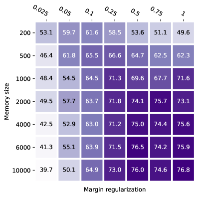
(a)

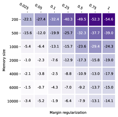
(b)

Figure 3: How the accuracy (left) and the BTW (right) scores are affected when varying the memory and the past margin regularisation. The results were obtained on ResNet-20 trained on C10-5.

Here, we analyse how our approach controls the trade-off between plasticity and stability. The only parameter of our regularisation schema is $\lambda$, which is combined with the size of the memory to achieve the desired trade-off. Figure 3 shows the results of training a ResNet-20 on the C10-5 scenario.

Even when operating with small memories, it is possible to combine these values to achieve the best stability-plasticity trade-off. For example, combining a small memory (e.g. 200) with a high regularisation term (higher than 0.1) leads to bad results, since the memory does not contain enough samples to balance the forgetting. However, better results can be achieved when the regularisation term is $0.1$ or lower, giving the best results for such a combination of memory size and the regularisation term, and showing that a good trade-off can be easily obtained. These findings suggest that increasing the size of the memory allows for a stronger regularisation term, and such a combination improves the results. These findings are confirmed by the results shown in Figure 3.

On the other hand, having a low regularisation term (e.g., 0.01) leads to a training schema focused on the stability of the model, which is incapable of properly learning current classes when using any memory size. Such combinations lead to a low BWT as well as a low accuracy, symptoms that current tasks are not learned properly due to the high focus on stability preservation.

In the end, such results show that, as opposed to other approaches, the choice of the regularisation term $\lambda$ and the memory size affect the achievable results predictably. These two quantities are easy to balance, resulting in better results overall.

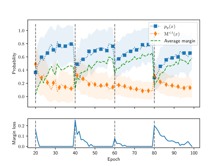
Figure 4: The figure (up) shows how the past logits, as well as the ground truth ones and the margin loss (down), vary during the training from the second task onward. Results were obtained on ResNet-20 trained on C10-5, with 500 samples saved in the memory and our proposal as the regularisation method.

4.3.2 MD regularisation effects

Figure 4 shows how the probabilities change when training the model using the proposed Margin Dampening regularisation approach. As we can see in the top image, the ground truth probabilities constantly increase while, at the same time, the maximum probabilities from past tasks decrease. The regularisation loss reaches zero after a few epochs, showing the regularisation ability of the proposed approach. Despite that, the maximum past value associated with current training samples keeps reducing even after the loss reaches zero (due to the soft constraint imposed by the Equation (4)). Such decreasing does not affect the output produced for past samples since the constraint imposed by the regularisation term is already respected, zeroing the regularisation term.

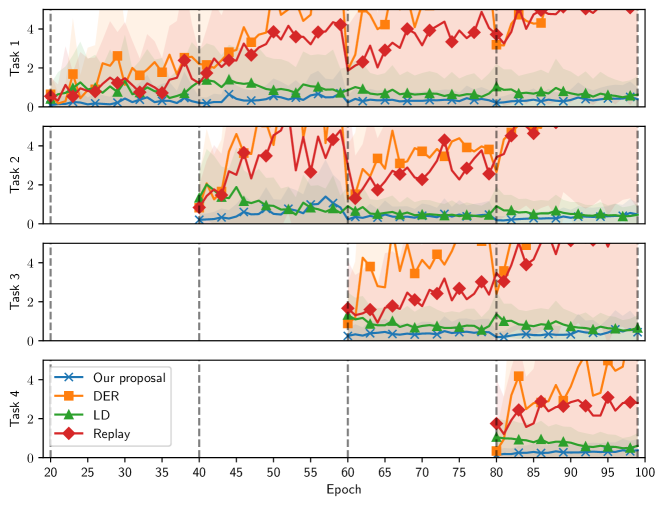
Figure 5: The images show the KL distance between the distributions predicted for past samples when a new task is collected and while training on it. The results are calculated over the whole test set of the C10-5 scenario, using the best hyperparameters and a memory size of 500.

4.3.3 Regularising future classes

Using past samples as training ones seems important to avoid learning current classes $\mathrm{Y}^{t}$ using only current task samples, called positive samples, which inevitably leads to CF. Moreover, we know that using such samples to augment the training procedure could lead to overfitting, increasing forgetting. Instead, we advocate that training on such samples is unnecessary and that future classes, concerning a past class $t^{\prime}<t$, can be easily regularised instead of trained, that improves both the plasticity and the stability. Here, we show this aspect by evaluating how the predictive ability of the model changes while training on newer tasks. Each time a new task $t$ is collected, we calculate the distribution $p^{t}_{0}(x)\in\mathbb{R}^{\lvert\mathcal{Y}^{t}\rvert}$, for all $x\in\mathcal{D}^{t^{\prime}}_{\text{test}}$ and for each $t^{\prime}<t$. Then, we evaluate how such distributions change while training on $t$ using the KL divergence between the current distributions and $p^{t}_{0}(x)$.

Figure 5 shows such results for DER, Replay, LD, and our proposal. DER, which uses a fixed number of output classes, regularised and trained simultaneously, diverges. Such behaviour is unsurprising as the approach trains all the future classes using only positive samples and then tries to keep the output of the model fixed while training it, negatively impacting the stability. Consequently, it must strike a delicate and hard-to-tune balance to work efficiently. Even then, ER-ACE and ER-LODE achieve better results. Since we observe the same divergence when using Replay, we conclude that DER regularisation has a negligible effect on future classes. On the other hand, LD can preserve the model’s predictive ability by keeping the divergence low during training. However, as seen in the main results, it lacks plasticity, resulting in low scores. Instead, our main proposal removes the overfitting by not training on past samples and by using a regularisation schema that allows for more plasticity without detriment to the stability. Ultimately, our main proposal is the only rehearsal-regularisation approach capable of preserving the model’s predictive capability while allowing for a higher degree of plasticity. These aspects combined lead to higher results overall, as already shown in the main results.

4.3.4 On scaling the Sigmoid function

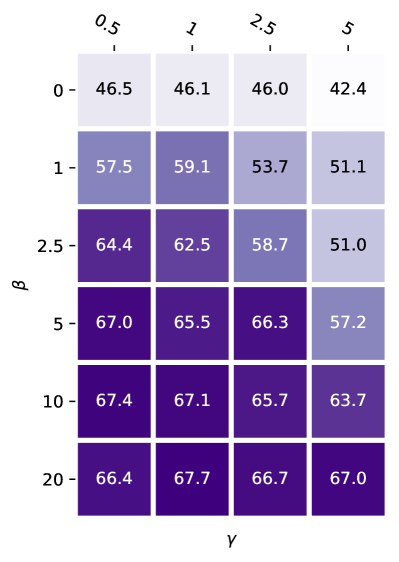
(a)

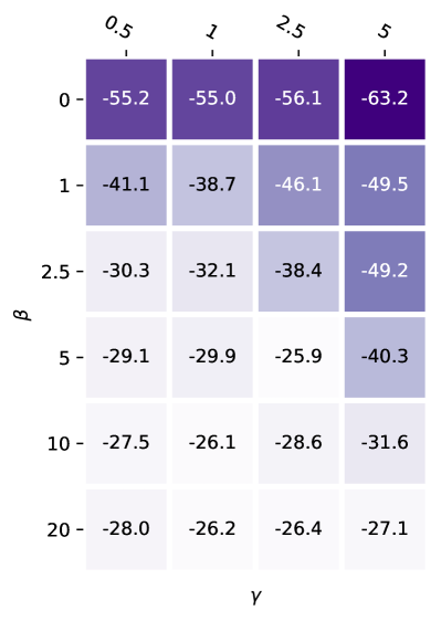
(b)

Figure 6: How the accuracy (left) and the BTW (right) scores are affected when varying the parameters of the scaler function proposed in Section 3.2. The results were obtained on ResNet-20 trained on C10-5 with a memory size set to 500.

In this section, we analyse how the scale ($\gamma$) and the offset ($\beta$) values used in the scaling function, proposed in Section 3.2, affect the results. Intuitively, a strong offset $\beta$ is necessary, since a high value will preserve past logits by not gating them at the beginning of the training, creating a model which is capable of outputting a distribution that resembles the one obtained by the model before starting the training on a new task. As shown in Fig. 6, a low offset value leads to a lower accuracy, which is partially recovered when the scaling value is lower than $1$. This is expected since a low offset does not guarantee that the model is regularised using the correct output distributions. Regarding the scaling value, which controls the smoothness of the Sigmoid curve, it behaves like a balance factor when the offset is below or equal to $2.5$, but it becomes less impacting as the offset gets higher, having a negligible impact when the latter reaches $20$. For this reason, in our experiment, we fixed the offset to 10 and the scale to 1.

4.3.5 Cascaded Scaling Classifier ablations

In this section, we analyse how much the proposed classifier CSC affects the results. To this end, we compare our proposal when the scaling functions in the set $S^{t}(x)$ are used (as in the main experiments) or not (which is, basically, an incremental classifier). Moreover, to understand if CSC could improve other approaches, we compare also the results achieved by ER-ACE when using or not the CSC classifier.

Figure 7 contains the results of both experiments. Looking at the ER-ACE results, we can see that our approach is capable of marginally improving the accuracy with respect to the counterpart that uses a standard incremental head classifier, especially when the memory size is contained; this effect is less visible when its dimension grows. Regarding our approach, the results are worse when the logits are not scaled, regardless of the memory size. However, the results are always better than ER-ACE. Intuitively, this happens because the scaling approach helps to mitigate the class unbalancing issue by giving the training procedure two ways to decrease past logits: by directly decreasing them or by decreasing the scaling value. This improves the plasticity without negatively affecting the stability, leading to better results. These aspects make our proposal competitive over all the benchmarks selected, with all possible combinations of memory size.

5 Conclusion

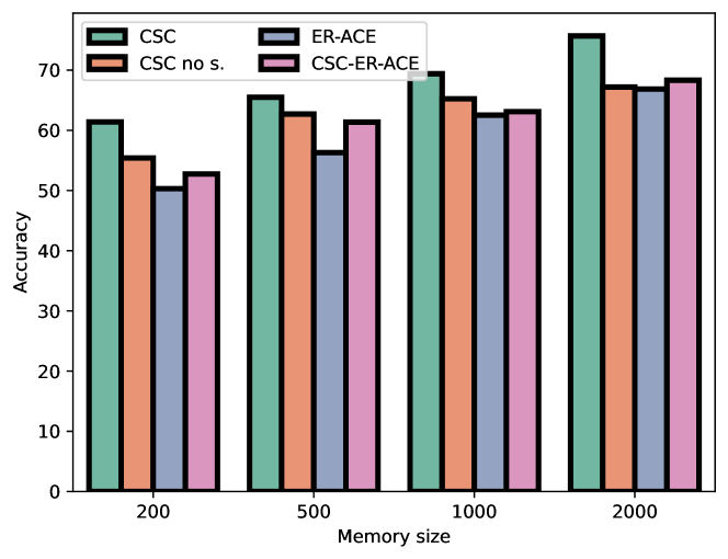
Figure 7: The results obtained on C10-5 when using (CSC) or not (CSC no s.) the scaling function $s(\cdot)$. In addition to this, the accuracy results obtained when using our proposed classifier (CSC) along ER-ACE, or not, are shown.

We proposed a novel rehearsal-regularisation approach which combines a constraint-based regularisation schema and a scaled classifier head, which builds the final prediction vector using a cascaded approach. Combining these components creates a CL method which achieves better results than the baselines. Our approach takes advantage of a soft constraint, which allows for smoother regularisation and less forgetting, even when an external memory contains few samples per class. We also extensively evaluated our proposal, to understand how and why the components affect the results. In the future, we will delve more into the theoretical analysis of class unbalancing mitigation in CL, which we empirically observed and shown in the paper. We will also extend the approach for CL scenarios in which the task boundaries are not well defined, as well as Online CL scenarios.

6 Impact Statement

This paper presents work whose goal is to advance the field of Continual Learning. Although our work could have potential societal consequences, we feel that none of these must be specifically highlighted here.

Appendix A Regularising and learning on past samples

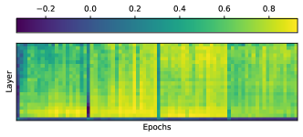
Figure 8: The cosine distance between gradients produced by the loss calculated on rehearsal samples and the ones related to the Knowledge Distillation regularisation. The last layer (last row of the heatmap) is the one which constantly has the two gradients pointing toward different directions.

We hypothesize that a hybrid approach which, at the same time, uses rehearsal samples as training samples as well as regularisation ones is sub-optimal. Figure 8 shows how the gradients diverge when using DER (Buzzega et al., 2020), when training Resnet-20 on C10-5, with a memory having a size of 500. The image shows the difference, calculated over the output channels, between the gradients obtained using the standard cross entropy and the one obtained for the knowledge distillation regularisation, both calculated over samples in the memory.

We can see that the method produces classification layer’s gradients giving negative similarity, suggesting that the two terms of the training loss try to move the model towards two different directions: in the first one the model satisfies the cross entropy (with the risk of overfitting over past samples), while the second one tries to keep the logits fixed. Even if competitive results are achievable by carefully balancing the loss terms, we advocate that the final results are highly sub-optimal.

Appendix B Related work

Existing CL approaches can be mainly categorised into three categories, even if, most of the time, an approach can belong to multiple categories at the same time. Regularisation approaches (Kirkpatrick et al., 2017; Zenke et al., 2017; Aljundi et al., 2018; Ahn et al., 2021; Chaudhry et al., 2021; Frascaroli et al., 2023; Gomez-Villa et al., 2022) introduce additional terms in the loss function to force the model to preserve knowledge that is crucial to keep solving past learned tasks while learning to solve newer ones. Architectural approaches (Rusu et al., 2016; Mallya & Lazebnik, 2018; Golkar et al., 2019; Douillard et al., 2020; Pomponi et al., 2021; Zhai et al., 2023; Wortsman et al., 2020) directly operate on the model itself, by isolating weights or dynamically expanding the model capacity. Rehearsal-based approaches implement an external memory containing examples from prior tasks and usually train the model jointly with the current task (Buzzega et al., 2020; Chaudhry et al., 2019; Prabhu et al., 2020; Pham et al., 2023; Wang et al., 2022; Xu et al., 2023; Bang et al., 2021; Pomponi et al., 2021). A subset of such methods is called Pseudo-rehearsal, in which a generative model takes the place of the memory (Van de Ven et al., 2020; Lao et al., 2020; Mundt et al., 2022; Gao & Liu, 2023; Pomponi et al., 2023). Although generative models are susceptible to issues like forgetting and mode collapse, they overcome the lack of diversity present in bounded memory buffers.

Appendix C Baselines

In this section, we list all the baselines we compared our proposal with. The selected baselines are:

Experience Replay (Chaudhry et al., 2019; Buzzega et al., 2021): it is a simple rehearsal approach, in which samples from the memory are used along with the ones from the current dataset to train the model. It has a fixed-sized memory populated with samples from the current task once it is over, discarding past samples to make room for newer ones.

Greedy Sampler and Dumb learner (GDumb) (Prabhu et al., 2020): it was proposed for questioning the advantages of CL, and it simply avoids training the model when a new task is collected, which is just used to fill up the memory. The just-filled memory is then used to train a new model from scratch when needed.

Experience Replay with Asymmetric Cross-Entropy (ER-ACE) (Caccia et al., 2022): initially proposed for contrasting CF in an Online CL scenario, it was also adapted for CIL. It uses a disjointed cross-entropy loss to leverage class unbalancing.

Separated Softmax for Incremental Learning (SS-IL) (Ahn et al., 2021): it mitigates the CF using Knowledge Distillation on a task-wise basis, in addition to a modified cross-entropy loss to learn patterns from the current task.

Gradient Episodic Memory (GEM) (Lopez-Paz & Ranzato, 2017): it uses the external memory to calculate gradients associated with past tasks and uses them to move the current one in a region of the space that satisfies both the current task as well as past ones. It does so by minimizing a quadratic problem, whose computational complexity scales exponentially with the number of samples in the memory.

Dark experience replay (DER) (Buzzega et al., 2020): the model is regularised by, at the same time, augmenting the current batch using past samples and regularizing the logits using the MSE distance loss between the logits obtained using the current model and the ones from the past model. The approach implements a classifier with a fixed number of classes, trained all at the same time.

Regular Polytope Classifier (RPC) (Pernici et al., 2021): the idea is to fight the CF by using a fixed number of equidistant and not learnable classifiers, and to learn only the backbone. To avoid setting the number of classes in advance we add a projection layer, which produces a vector containing 1000 features, between the backbone and the classifier layer, fixing the number of learnable classes to 1001.

Loss Decoupled (ER-LODE) (Liang & Li, 2023): it decouples the classification loss creating two components conditional on whether the samples are from the current task or not. It uses an external memory and combines the losses by weighting them using a scaling factor which depends on the number of seen classes.

Logits Distillation (LD): we also propose a simple baseline called Logits Distillation, in which an external class-balanced memory contains images used to regularize the logits with a KL distance (weighted by a constant $\alpha$). To do so, a copy of the model, used as the teacher model, is created at the beginning of the training. Moreover, we regularize future logits as in our proposed method (Section 3.1). This baseline is useful for studying the effect of future regularisation without involving any classification loss over past samples.

Appendix D Hyperparameters selection

Dataset	Method	Memory size
		200	500	1000	2000	5000
C10-5	DER	$\alpha=0.1,\beta=0.5$	$\alpha=0.5,\beta=0.8$	$\alpha=0.5,\beta=0.1$	$\alpha=0.2,\beta=0.8$
	LODE	$\rho=0.2$	$\rho=0.5$
	LD	$\alpha=0.1$
	MARGIN	$\lambda=0.1$	$\lambda=0.25$		$\lambda=0.5$
C100-10	DER	$\alpha=0.1,\beta=0.8$	$\alpha=0.1,\beta=1$	$\alpha=0.1,\beta=0.8$
	LODE	$\rho=0.1$	$\rho=0.2$		$\rho=0.5$
	LD	$\alpha=1$		$\alpha=0.75$
	MARGIN	$\lambda=0.1$	$\lambda=0.5$	$\lambda=0.25$	$\lambda=1$
TyN-10	DER	$\alpha=0.1,\beta=0.5$	$\alpha=0.1,\beta=0.1$	$\alpha=0.1,\beta=0.5$	$\alpha=0.1,\beta=0.2$
	LODE	$\rho=0.1$			$\rho=0.2$	$\rho=0.5$
	LD	$\alpha=1$	$\alpha=0.5$	$\alpha=1$		$\alpha=0.75$
	MARGIN	$\lambda=0.05$			$\lambda=0.25$

Table 2: The best combination of hyper-parameters for each approach.

To select the best hyperparameters, we fixed the number of epochs, the batch size, and the optimizer parameters. Then, we trained a model for each combination of hyperparameters, and we selected the best set by evaluating the results on a development split containing $10\%$ of the training samples. For each method, the hyperparameters are:

• DER (Buzzega et al., 2020): this approach has two hyperparameters. The first controls the classification loss of past samples, $\alpha:[0.1,0.2,0.5,0.8,1.0]$, while the second controls the logits distillation loss $\beta:[0.1,0.2,0.5,0.8,1.0]$.

• LODE (Liang & Li, 2023): the only parameter $\rho$ controls the weight of the proportion between the number of new classes over the number of past ones. The resulting value is used to weigh one of the losses. Based on the findings shown in the paper, the search space is $\rho:[0.1,0.2,0.5,0.8,1]$.

• LD: it has just one parameter, which controls the strength of the logit regularisation. The search space is $\alpha:[0.1,0.25,0.5,0.75,1]$

• MD: our proposal has only one hyperparameter, which controls the strength of margin regularisation, and the search space is $\lambda:[1,0.5,0.25,0.1,0.05,0.025,0.01]$.

The best parameters, for each combination of scenario and memory, are shown in Table 2.

Appendix E Metrics

To evaluate the efficiency of a CL method, we use two different metrics proposed in (Díaz-Rodríguez et al., 2018). The first one, called Accuracy, shows the final accuracy obtained across all the tasks’ test splits, while the second one, called Backward Transfer (BWT), measures how much of that past accuracy is lost during the training on upcoming tasks. To calculate the metrics, we use a matrix $\mathbf{R}\in\mathbb{R}^{\text{N}\times\text{N}}$, in which an entry $\mathbf{R}_{i,j}$ is the test accuracy obtained on the test split of the task $j$ when the training on the task $i$ is over. Using the matrix $\mathbf{R}$ we calculate the metrics as:

$$\text{ACC}=\frac{1}{\text{\text{N}}}\sum_{j=1}^{\text{\text{N}}}\mathbf{R}_{\text{\text{N}},j}$$

$$\text{BWT}=\frac{\sum_{i=2}^{\text{\text{N}}}\sum_{j=1}^{i-1}(\mathbf{R}_{i,j}-\mathbf{R}_{j,j})}{\frac{1}{2}\text{\text{N}}(\text{\text{N}}-1)}\,.$$

Both metrics are important to evaluate a CL method since a low BWT does not imply that the model performs well, especially if we also have a low Accuracy score because, in that case, it means that the approach regularizes too much during the training, leaving no space for learning new tasks. In the end, the combination of the metrics is what we need to evaluate.

References

- Ahn et al. (2021) Ahn, H., Kwak, J., Lim, S., Bang, H., Kim, H., and Moon, T. Ss-il: Separated softmax for incremental learning. In Proceedings of the IEEE/CVF International conference on computer vision, pp. 844–853, 2021.
- Aljundi et al. (2018) Aljundi, R., Babiloni, F., Elhoseiny, M., Rohrbach, M., and Tuytelaars, T. Memory Aware Synapses: Learning What (not) to Forget, pp. 144–161. Springer International Publishing, 2018.
- Bang et al. (2021) Bang, J., Kim, H., Yoo, Y., Ha, J.-W., and Choi, J. Rainbow memory: Continual learning with a memory of diverse samples. In Proceedings of the IEEE/CVF conference on computer vision and pattern recognition, pp. 8218–8227, 2021.
- Bonicelli et al. (2022) Bonicelli, L., Boschini, M., Porrello, A., Spampinato, C., and Calderara, S. On the effectiveness of lipschitz-driven rehearsal in continual learning. Advances in Neural Information Processing Systems, 35:31886–31901, 2022.
- Buzzega et al. (2020) Buzzega, P., Boschini, M., Porrello, A., Abati, D., and Calderara, S. Dark experience for general continual learning: a strong, simple baseline. Advances in neural information processing systems, 33:15920–15930, 2020.
- Buzzega et al. (2021) Buzzega, P., Boschini, M., Porrello, A., and Calderara, S. Rethinking experience replay: a bag of tricks for continual learning. In 2020 25th International Conference on Pattern Recognition (ICPR), pp. 2180–2187. IEEE, 2021.
- Caccia et al. (2022) Caccia, L., Aljundi, R., Asadi, N., Tuytelaars, T., Pineau, J., and Belilovsky, E. New insights on reducing abrupt representation change in online continual learning. In International Conference on Learning Representations, 2022.
- Chaudhry et al. (2019) Chaudhry, A., Rohrbach, M., Elhoseiny, M., Ajanthan, T., Dokania, P. K., Torr, P. H., and Ranzato, M. On tiny episodic memories in continual learning. arXiv preprint arXiv:1902.10486, 2019.
- Chaudhry et al. (2021) Chaudhry, A., Gordo, A., Dokania, P., Torr, P., and Lopez-Paz, D. Using hindsight to anchor past knowledge in continual learning. In Proceedings of the AAAI conference on artificial intelligence, volume 35, pp. 6993–7001, 2021.
- Deng et al. (2009) Deng, J., Dong, W., Socher, R., Li, L.-J., Li, K., and Fei-Fei, L. Imagenet: A large-scale hierarchical image database. In 2009 IEEE Conference on Computer Vision and Pattern Recognition, pp. 248–255, 2009.
- Díaz-Rodríguez et al. (2018) Díaz-Rodríguez, N., Lomonaco, V., Filliat, D., and Maltoni, D. Don’t forget, there is more than forgetting: new metrics for continual learning. arXiv preprint arXiv:1810.13166, 2018.
- Douillard et al. (2020) Douillard, A., Cord, M., Ollion, C., Robert, T., and Valle, E. Podnet: Pooled outputs distillation for small-tasks incremental learning. In Computer Vision–ECCV 2020: 16th European Conference, pp. 86–102. Springer, 2020.
- Frascaroli et al. (2023) Frascaroli, E., Benaglia, R., Boschini, M., Moschella, L., Fiorini, C., Rodolà, E., and Calderara, S. Casper: Latent spectral regularization for continual learning. arXiv preprint arXiv:2301.03345, 2023.
- Gao & Liu (2023) Gao, R. and Liu, W. Ddgr: Continual learning with deep diffusion-based generative replay. In Proceedings of the 40th International Conference on Machine Learning, ICML’23. JMLR.org, 2023.
- Golkar et al. (2019) Golkar, S., Kagan, M., and Cho, K. Continual learning via neural pruning. In Real Neurons & Hidden Units: Future directions at the intersection of neuroscience and artificial intelligence @ NeurIPS 2019, 2019.
- Gomez-Villa et al. (2022) Gomez-Villa, A., Twardowski, B., Yu, L., Bagdanov, A. D., and van de Weijer, J. Continually learning self-supervised representations with projected functional regularization. In Proceedings of the IEEE/CVF Conference on Computer Vision and Pattern Recognition, pp. 3867–3877, 2022.
- He et al. (2016) He, K., Zhang, X., Ren, S., and Sun, J. Deep residual learning for image recognition. In Proceedings of the IEEE conference on computer vision and pattern recognition, pp. 770–778, 2016.
- Kirkpatrick et al. (2017) Kirkpatrick, J., Pascanu, R., Rabinowitz, N., Veness, J., Desjardins, G., Rusu, A. A., Milan, K., Quan, J., Ramalho, T., Grabska-Barwinska, A., Hassabis, D., Clopath, C., Kumaran, D., and Hadsell, R. Overcoming catastrophic forgetting in neural networks. Proceedings of the National Academy of Sciences, 114(13):3521–3526, 2017. ISSN 1091-6490.
- Lao et al. (2020) Lao, Q., Jiang, X., Havaei, M., and Bengio, Y. Continuous domain adaptation with variational domain-agnostic feature replay. arXiv preprint arXiv:2003.04382, 2020.
- Li & Hoiem (2017) Li, Z. and Hoiem, D. Learning without forgetting. IEEE transactions on pattern analysis and machine intelligence, 40(12):2935–2947, 2017.
- Liang & Li (2023) Liang, Y.-S. and Li, W.-J. Loss decoupling for task-agnostic continual learning. In Thirty-seventh Conference on Neural Information Processing Systems, 2023.
- Lomonaco et al. (2021) Lomonaco, V., Pellegrini, L., Cossu, A., Carta, A., Graffieti, G., Hayes, T. L., De Lange, M., Masana, M., Pomponi, J., Van de Ven, G. M., et al. Avalanche: an end-to-end library for continual learning. In Proceedings of the IEEE/CVF Conference on Computer Vision and Pattern Recognition, pp. 3600–3610, 2021.
- Lopez-Paz & Ranzato (2017) Lopez-Paz, D. and Ranzato, M. Gradient episodic memory for continual learning. Advances in neural information processing systems, 30, 2017.
- Mallya & Lazebnik (2018) Mallya, A. and Lazebnik, S. Packnet: Adding multiple tasks to a single network by iterative pruning. In Proceedings of the IEEE conference on Computer Vision and Pattern Recognition, pp. 7765–7773, 2018.
- Mundt et al. (2022) Mundt, M., Pliushch, I., Majumder, S., Hong, Y., and Ramesh, V. Unified probabilistic deep continual learning through generative replay and open set recognition. Journal of Imaging, 8(4), 2022.
- Parisi et al. (2019) Parisi, G. I., Kemker, R., Part, J. L., Kanan, C., and Wermter, S. Continual lifelong learning with neural networks: A review. Neural Networks, 113:54–71, 2019.
- Pernici et al. (2021) Pernici, F., Bruni, M., Baecchi, C., Turchini, F., and Del Bimbo, A. Class-incremental learning with pre-allocated fixed classifiers. In 2020 25th International Conference on Pattern Recognition (ICPR), pp. 6259–6266. IEEE, 2021.
- Pham et al. (2023) Pham, Q., Liu, C., and Hoi, S. C. Continual learning, fast and slow. IEEE Transactions on Pattern Analysis and Machine Intelligence, 2023.
- Pomponi et al. (2021) Pomponi, J., Scardapane, S., and Uncini, A. Structured ensembles: An approach to reduce the memory footprint of ensemble methods. Neural Networks, 144:407–418, 2021. ISSN 0893-6080.
- Pomponi et al. (2022) Pomponi, J., Scardapane, S., and Uncini, A. Centroids matching: an efficient continual learning approach operating in the embedding space. Transactions on Machine Learning Research, 2022. ISSN 2835-8856.
- Pomponi et al. (2023) Pomponi, J., Scardapane, S., and Uncini, A. Continual learning with invertible generative models. Neural Networks, 164:606–616, 2023.
- Prabhu et al. (2020) Prabhu, A., Torr, P. H., and Dokania, P. K. Gdumb: A simple approach that questions our progress in continual learning. In Computer Vision–ECCV 2020: 16th European Conference, Glasgow, UK, August 23–28, 2020, Proceedings, Part II 16, pp. 524–540. Springer, 2020.
- Rusu et al. (2016) Rusu, A. A., Rabinowitz, N. C., Desjardins, G., Soyer, H., Kirkpatrick, J., Kavukcuoglu, K., Pascanu, R., and Hadsell, R. Progressive neural networks. arXiv preprint arXiv:1606.04671, 2016.
- Van de Ven et al. (2020) Van de Ven, G. M., Siegelmann, H. T., and Tolias, A. S. Brain-inspired replay for continual learning with artificial neural networks. Nature communications, 11(1):4069, 2020.
- Verwimp et al. (2021) Verwimp, E., De Lange, M., and Tuytelaars, T. Rehearsal revealed: The limits and merits of revisiting samples in continual learning. In 2021 IEEE/CVF International Conference on Computer Vision (ICCV). IEEE, 2021.
- Wang et al. (2023) Wang, L., Zhang, X., Su, H., and Zhu, J. A comprehensive survey of continual learning: Theory, method and application. arXiv preprint arXiv:2302.00487, 2023.
- Wang et al. (2022) Wang, Z., Zhan, Z., Gong, Y., Yuan, G., Niu, W., Jian, T., Ren, B., Ioannidis, S., Wang, Y., and Dy, J. Sparcl: Sparse continual learning on the edge. Advances in Neural Information Processing Systems, 35:20366–20380, 2022.
- Wortsman et al. (2020) Wortsman, M., Ramanujan, V., Liu, R., Kembhavi, A., Rastegari, M., Yosinski, J., and Farhadi, A. Supermasks in superposition. Advances in Neural Information Processing Systems, 33:15173–15184, 2020.
- Wu et al. (2019) Wu, Y., Chen, Y., Wang, L., Ye, Y., Liu, Z., Guo, Y., and Fu, Y. Large scale incremental learning. In Proceedings of the IEEE/CVF conference on computer vision and pattern recognition, pp. 374–382, 2019.
- Xu et al. (2023) Xu, Z., Tang, X., Shi, Y., Zhang, J., Yang, J., Chen, M., and Wei, X. Continual learning via manifold expansion replay. arXiv preprint arXiv:2310.08038, 2023.
- Zenke et al. (2017) Zenke, F., Poole, B., and Ganguli, S. Continual learning through synaptic intelligence. In International conference on machine learning, pp. 3987–3995. PMLR, 2017.
- Zhai et al. (2023) Zhai, J.-T., Liu, X., Bagdanov, A. D., Li, K., and Cheng, M.-M. Masked autoencoders are efficient class incremental learners. In Proceedings of the IEEE/CVF International Conference on Computer Vision, pp. 19104–19113, 2023.
- Zhao et al. (2020) Zhao, B., Xiao, X., Gan, G., Zhang, B., and Xia, S.-T. Maintaining discrimination and fairness in class incremental learning. In Proceedings of the IEEE/CVF conference on computer vision and pattern recognition, pp. 13208–13217, 2020.