Transformers Learn Nonlinear Features In Context:
Nonconvex Mean-field Dynamics on the Attention Landscape

Abstract

Large language models based on the Transformer architecture have demonstrated impressive capabilities to learn in context. However, existing theoretical studies on how this phenomenon arises are limited to the dynamics of a single layer of attention trained on linear regression tasks. In this paper, we study the optimization of a Transformer consisting of a fully connected layer followed by a linear attention layer. The MLP acts as a common nonlinear representation or feature map, greatly enhancing the power of in-context learning. We prove in the mean-field and two-timescale limit that the infinite-dimensional loss landscape for the distribution of parameters, while highly nonconvex, becomes quite benign. We also analyze the second-order stability of mean-field dynamics and show that Wasserstein gradient flow almost always avoids saddle points. Furthermore, we establish novel methods for obtaining concrete improvement rates both away from and near critical points. This represents the first saddle point analysis of mean-field dynamics in general and the techniques are of independent interest.

1 Introduction

Attention-based neural architectures such as Transformers have revolutionized modern machine learning, from tasks in natural language and computer vision to multi-modal learning and beyond. Recently, interest has surged in the remarkable ability of large language models to learn in context, leading to a major paradigm shift in how intelligence arises in artificial systems. In-context learning (ICL) refers to the capacity of a pretrained model to solve previously unseen tasks based on example prompts without further tuning its parameters.

A vigorous line of research initiated by Garg et al. (2022) has sought to understand the mechanism behind ICL from a theoretical perspective, where prompts are real-valued input-output pairs $(x_{i},f(x_{i}))_{i=1}^{n}$ generated from some function class $\operatorname{\mathscr{T}}$. Studies have shown that Transformers are capable of implementing various statistical learning algorithms such as gradient descent (GD) in context (von Oswald et al., 2023; Akyürek et al., 2023; Bai et al., 2023). In particular, Guo et al. (2023) consider the realistic setting of learning with representations where MLP layers act as transformations on top of which ICL is performed, and show that such models consistently achieve near-optimal performance.

While promising, these results are based on specific constructions which may not accurately reflect ICL in real models (Shen et al., 2023). Other works have analyzed how ICL emerges from the training dynamics of Transformers (Zhang et al., 2023a; Huang et al., 2023; Ahn et al., 2023a). However, they are limited to models consisting of only a single attention layer due to the challenging dynamical complexity and thus can only explain ICL of linear functions. Hence the following central question at the intersection of the two approaches remains unsolved:

How does in-context learning with nonlinear representations (features) arise in Transformers with
MLP layers, optimized via gradient descent?

In this paper, we investigate a Transformer consisting of a two-layer MLP followed by a linear attention layer pretrained on linear transformations of feature representations. Contrary to existing approaches which attempt to solve for exact dynamics of the attention matrices, we factor out the attention layer via a two-timescale argument and focus on the loss landscape faced by an overparametrized MLP. Our contributions are highlighted as follows.

• We show that the MLP layer greatly increases the flexibility of ICL by extending the class of learnable functions to the Barron space and plays an essential role by encoding task-common features during pretraining.

• Lifting to the mean-field regime, we show that this infinite-dimensional ‘attention landscape’ is benign (strictly saddle) via directional analysis: all critical points are either global minima or saddle points.

• We formally prove that mean-field dynamics (MFD) ‘almost always’ avoids saddle points, explaining how the MLP can find globally optimal representations. We analyze local stability of Wasserstein gradient flow on the space of measures using tools from Otto calculus, optimal transport and functional analysis.

• We further derive concrete improvement rates in three regions under slightly modified dynamics: away from saddle points, near global minima and near saddle points. For the last case, we discuss how perturbed dynamics may help ensure global convergence rates.

While the benignity established in Section 3 is our central insight into ICL, Sections 4 and 5 constitute the first qualitative and quantitative convergence analyses of nonconvex mean-field dynamics around saddle points and is also of significant interest from a technical standpoint. We present many novel results for general functionals and outline another application to three-layer neural networks. Finally, we conduct numerical experiments complementing our theory.

1.1 Related Works

In-context learning.

A wide literature has developed around the various aspects of ICL; we only mention those most relevant to our setup. Akyürek et al. (2023); von Oswald et al. (2023); Mahankali et al. (2023) give a construction where a single linear attention layer is equivalent to one step of GD or ridge regression. Transformers are also capable of implementing statistical (Bai et al., 2023) and reinforcement learning algorithms (Lin et al., 2023) and model averaging (Zhang et al., 2023b). The attention-over-representation viewpoint has been studied by Guo et al. (2023) and also Tsai et al. (2019); Han et al. (2023) from a kernel regression perspective. Zhang et al. (2023a) analyze the optimization of a linear attention-only Transformer and show global convergence; a relationship to preconditioned GD is established in Ahn et al. (2023a). Also, Huang et al. (2023) give a stage-wise analysis for the softmax attention-only model. Finally, a joint dynamic framework for MLP and attention has been proposed in Tian et al. (2023).

Mean-field dynamics.

Let $h_{\theta}$ denote a single neuron with parameter $\theta\in\Omega\subseteq\operatorname{\mathbb{R}}^{m}$ and $\operatorname{\mathscr{P}}(\Omega)$ the space of probability measures over $\Omega$. In the infinite-width limit, a two-layer neural network $h_{N}(\bm{x})=\frac{1}{N}\sum_{j=1}^{N}h_{\theta^{(j)}}(\bm{x})$ can be written as an expectation $h_{\mu}(\bm{x})=\mathbb{E}_{\theta\sim\mu}[h_{\theta}(\bm{x})]$ over a distribution $\mu\in\operatorname{\mathscr{P}}(\Omega)$. The corresponding mean-field limit of gradient flow (GF) w.r.t. an objective function $F:\operatorname{\mathscr{P}}(\Omega)\to\operatorname{\mathbb{R}}$, the Wasserstein gradient flow (Jordan et al., 1998), is given by the continuity equation

$$\textstyle\partial_{t}\mu_{t}=\nabla\cdot\left(\mu_{t}\nabla\frac{\delta F}{\delta\mu}(\mu_{t})\right),\quad t\geq 0.$$ (1)

Networks in this regime are capable of dynamic feature learning and convergence, compared to the NTK regime where the underlying kernel is essentially frozen. Works such as Chizat & Bach (2018); Mei et al. (2018); Nitanda et al. (2022) exploit the linearity of $h_{\mu}$ in $\mu$ and the convexity of the loss to lift to a convex optimization problem on $\operatorname{\mathscr{P}}(\Omega)$ and obtain convergence results. In contrast, the ICL loss is inherently nonconvex due to the additional attention layer.

Landscape analyses.

Certain nonconvex objectives such as matrix completion, sensing and factorization have been proved to be benign via directional analysis (Ge et al., 2016, 2017; Li et al., 2019). Recently, Gaussian $k$-index models have been shown to possess benign landscapes w.r.t. the projection matrix after factoring out the link function via a similar two-timescale limit (Bietti et al., 2023). However, our work focuses on the optimization of the infinite-dimensional variable $\mu\in\operatorname{\mathscr{P}}(\Theta)$, and the ICL objective (3) has a novel, more complex structure compared to these problems.

Theoretical preliminaries are provided in Appendix A, and proofs of all results in Sections 2-5 are given throughout Appendices B-E.

2 In-Context Feature Learning

Notation.

We denote both the $L^{2}$-norm of vectors and spectral norm of matrices by $\lVert\cdot\rVert$ and the nuclear norm by $\lVert\cdot\rVert_{*}$. The unit ball in $\operatorname{\mathbb{R}}^{k}$ is written as $\mathbb{D}^{k}=\{\bm{z}\in\operatorname{\mathbb{R}}^{k}:\lVert\bm{z}\rVert\leq 1\}$. The unit ball in $\operatorname{\mathbb{R}}^{k\times k}$ with respect to spectral norm is written as $\operatorname{\mathcal{B}}_{1}(k)=\{\mathbf{R}\in\operatorname{\mathbb{R}}^{k\times k}:\lVert\mathbf{R}\rVert\leq 1\}$. The orthogonal group in dimension $k$ is denoted by $\mathcal{O}(k)$. The $L^{2}$-norm of functions is explicitly written as $\lVert\cdot\rVert_{L^{2}}$.

2.1 Setup: In-Context Learning

The basic theoretical framework for studying ICL was first proposed by Garg et al. (2022) and has since been widely embraced (Bai et al., 2023; Zhang et al., 2023a; Ahn et al., 2023a; Huang et al., 2023; Lin et al., 2023; Wu et al., 2024). Let $\operatorname{\mathcal{D}}_{\operatorname{\mathscr{X}}}$ be a distribution over the input space $\operatorname{\mathscr{X}}\subseteq\operatorname{\mathbb{R}}^{d}$, and let $\operatorname{\mathscr{T}}$ be a class of functions $\operatorname{\mathscr{X}}\to\operatorname{\mathbb{R}}$ with a distribution $\operatorname{\mathcal{D}}_{\operatorname{\mathscr{T}}}$ over functions. For each prompt, we generate a new task $f\sim\operatorname{\mathcal{D}}_{\operatorname{\mathscr{T}}}$ and a batch of $n$ example input-output pairs $(\bm{x}_{i},y_{i})_{i=1}^{n}$ where $\bm{x}_{i}\sim\operatorname{\mathcal{D}}_{\operatorname{\mathscr{X}}}$ are i.i.d. and $y_{i}=f(\bm{x}_{i})$. We also independently generate a query token $\bm{x}_{\textup{qr}}\sim\operatorname{\mathcal{D}}_{\operatorname{\mathscr{X}}}$. The prompt is gathered into an embedding matrix

$$\mathbf{E}=\begin{bmatrix}\mathbf{E}^{\bm{x}}\\ \mathbf{E}^{y}\end{bmatrix}=\begin{bmatrix}\bm{x}_{1}&\cdots&\bm{x}_{n}&\bm{x}_{\textup{qr}}\\ y_{1}&\cdots&y_{n}&0\end{bmatrix}\in\operatorname{\mathbb{R}}^{(d+1)(n+1)}.$$

In-context learning of a pretrained model $\mathbb{M}$ refers to the ability to form predictions $\widehat{y}_{\textup{qr}}=\mathbb{M}(\mathbf{E})$ for $y_{\textup{qr}}=f(\bm{x}_{\textup{qr}})$ without knowledge of the current task $f$ and without updating its parameters.

2.2 MLP-Attention Transformer

We now formally define our Transformer model, which consists of a feedforward two-layer neural network (MLP) followed by a single linear self-attention (LSA) layer. This serves as a proxy of the original Transformer which consists of alternating feedforward and attention layers. As in Guo et al. (2023), we switch the conventional ordering of the two networks to view attention as a mechanism to exchange feature information encoded into the MLP layer (we may also consider the initial embedding as the first MLP layer).

MLP layer.

A vector-valued neuron with parameter $\theta=(\bm{a},\bm{w})^{\top}\in\Theta\subseteq\operatorname{\mathbb{R}}^{k}\times\operatorname{\mathbb{R}}^{d}$ and activation $\sigma:\operatorname{\mathbb{R}}\to\operatorname{\mathbb{R}}$ is defined as $h_{\theta}(\bm{x})=\bm{a}\sigma(\bm{w}^{\top}\bm{x})$. While the original Transformer takes $k=d$, we allow any $k\leq d$ representing the number of distinct features. The mean-field network corresponding to a measure $\mu\in\operatorname{\mathscr{P}}(\Theta)$ is defined as $\textstyle h_{\mu}(\bm{x})=\int_{\Theta}h_{\theta}(\bm{x})\mu(\mathop{}\!\mathrm{d}\theta)$. We will also denote $\bm{\Sigma}_{\mu,\nu}=\mathbb{E}_{\bm{x}\sim\operatorname{\mathcal{D}}_{\operatorname{\mathscr{X}}}}[h_{\mu}(\bm{x})h_{\nu}(\bm{x})^{\top}]\in\operatorname{\mathbb{R}}^{k\times k}$. As we wish to extract features from the input tokens, the MLP is applied to only the covariates $\bm{x}_{i}$ and $\bm{x}_{\textup{qr}}$ so that the prompt $\mathbf{E}$ is transformed into

$$\operatorname{MLP}(\mathbf{E})=\begin{bmatrix}h_{\mu}(\bm{x}_{1})&\cdots&h_{\mu}(\bm{x}_{n})&h_{\mu}(\bm{x}_{\textup{qr}})\\ y_{1}&\cdots&y_{n}&0\end{bmatrix}.$$

LSA layer.

Linear attention is widely used to accelerate the quadratic complexity of standard attention (Katharopoulos et al., 2020; Yang et al., 2023) and can capture various aspects of softmax attention (Ahn et al., 2023b) while still being theoretically amenable. For query, key and value matrices $\mathbf{W}^{Q},\mathbf{W}^{K},\mathbf{W}^{V}\in\operatorname{\mathbb{R}}^{(k+1)(k+1)}$ define

$$\textstyle\operatorname{LSA}(\mathbf{E})=\mathbf{W}^{V}\mathbf{E}\cdot\frac{1}{n}(\mathbf{W}^{K}\mathbf{E})^{\top}(\mathbf{W}^{Q}\mathbf{E}).$$

We impose a specific form, shown to achieve the global optimum in Zhang et al. (2023a); Mahankali et al. (2023), where the query and key matrices are consolidated into $\mathbf{W}\in\operatorname{\mathbb{R}}^{k\times k}$ and $\mathbf{W}^{V}$ is reduced to a scalar multiplier $v$:

$$\mathbf{W}^{V}=\begin{bmatrix}*&*\\ 0_{d}^{\top}&v\end{bmatrix},\quad(\mathbf{W}^{K})^{\top}\mathbf{W}^{Q}=\begin{bmatrix}\mathbf{W}&0_{d}\\ 0_{d}^{\top}&*\end{bmatrix}.$$

We further absorb $v$ into $\mathbf{W}$ and fix $v=1$ in order to focus on the more complex dynamics of the MLP layer. Corresponding to the position of $y_{\textup{qr}}$, the $(k+1,n+1)$th element of the output is read out as the model prediction. Multiplying out the matrices yields

$$\widehat{y}_{\textup{qr}}=\operatorname{LSA}\circ\operatorname{MLP}(\mathbf{E})=\frac{1}{n}\sum_{i=1}^{n}y_{i}h_{\mu}(\bm{x}_{i})^{\top}\mathbf{W}h_{\mu}(\bm{x}_{\textup{qr}}).$$

Hence $\widehat{y}_{\textup{qr}}$ can be interpreted as a linear smoother with the kernel $k(\bm{x},\bm{x}_{\textup{qr}})=\frac{1}{n}h_{\mu}(\bm{x})^{\top}\mathbf{W}h_{\mu}(\bm{x}_{\textup{qr}})$ encoded by the MLP layer (cf. Tsai et al. (2019) for softmax attention).

Regression over features.

In this paper, we study ICL of linear regression tasks over a common nonlinear transformation or feature map $f^{\circ}\in C(\operatorname{\mathscr{X}},\operatorname{\mathbb{R}}^{k})$, that is $\operatorname{\mathscr{T}}=\{\bm{v}^{\top}f^{\circ}|\,\bm{v}\in\operatorname{\mathbb{R}}^{k}\}$. We assume that during pretraining the tasks are suitably spread out with $\mathbb{E}_{\bm{v}}[\bm{v}\bm{v}^{\top}]=\mathbf{I}_{k}$; if some direction is not shown enough in context, there is no hope to learn all relevant features. We will also take the $n\to\infty$ (infinite prompt length) limit so that we can disregard sampling error and let $\widehat{y}_{\textup{qr}}=\mathbb{E}_{\bm{x}}[f(\bm{x})h_{\mu}(\bm{x})^{\top}]\mathbf{W}h_{\mu}(\bm{x}_{\textup{qr}})$ for any task $f\in\operatorname{\mathscr{T}}$. Hence our Transformer is pretrained with the following mean squared risk,

$$\operatorname{\mathcal{L}}_{\textup{TF}}(\mu,\mathbf{W}):=\frac{1}{2}\mathbb{E}_{\bm{x}_{\textup{qr}},\bm{v}}\left[(y_{\textup{qr}}-\widehat{y}_{\textup{qr}})^{2}\right]$$ (2)

$$=\frac{1}{2}\mathbb{E}_{\bm{x}_{\textup{qr}}}\left[\left\lVert f^{\circ}(\bm{x}_{\textup{qr}})-\mathbb{E}_{\bm{x}}[f^{\circ}(\bm{x})h_{\mu}(\bm{x})^{\top}]\mathbf{W}h_{\mu}(\bm{x}_{\textup{qr}})\right\rVert^{2}\right].$$

Our goal is to show that gradient dynamics converges to a global minimum such that $\operatorname{\mathcal{L}}_{\textup{TF}}=0$. Then the MLP layer has successfully learned the true representations $f^{\circ}$, and even for a new or ‘unseen’ task $\bm{v}_{\text{new}}\in\operatorname{\mathbb{R}}^{k}$ the Transformer is able to return the correct regression output $y_{\textup{qr}}$:

$$\widehat{y}_{\textup{qr}}=\mathbb{E}_{\bm{x}}[\bm{v}_{\textup{new}}^{\top}f^{\circ}(\bm{x})h_{\mu}(\bm{x})^{\top}]\mathbf{W}h_{\mu}(\bm{x}_{\textup{qr}})=\bm{v}_{\textup{new}}^{\top}f^{\circ}(\bm{x}_{\textup{qr}}).$$

We call this behavior in-context feature learning (ICFL).

2.3 Expressivity of Representations

Before delving into the training dynamics of our Transformer, we show by extending classical analyses of two-layer neural networks that adding even a shallow MLP results in greatly increased in-context learning capabilities, justifying our feature-based approach.

Multivariate Barron class.

Barron-type spaces have been well established as the natural function classes for analyzing approximation and generalization of shallow neural networks (Barron, 1994; Weinan et al., 2020; Weinan & Wojtowytsch, 2022). Here, we extend the theory to our vector-valued setting. We focus on the ReLU case for ease of presentation, but many results extend to more general activations (Klusowski & Barron, 2016; Li et al., 2020).

Set $\Theta=\operatorname{\mathbb{R}}^{k}\times\operatorname{\mathbb{R}}^{d}$, $\sigma(z)=\max\{0,z\}$ and suppose $M_{2}=\mathbb{E}_{\bm{x}\sim\operatorname{\mathcal{D}}_{\operatorname{\mathscr{X}}}}[\lVert\bm{x}\rVert^{2}]<\infty$. The Barron space $\operatorname{\mathscr{B}}_{p}$ of order $p\in[1,\infty]$ is defined as the set of functions $f=h_{\mu}$, $\mu\in\operatorname{\mathscr{P}}(\Theta)$ with finite Barron norm

$$\textstyle\lVert f\rVert_{\operatorname{\mathscr{B}}_{p}}:=\inf_{\mu:f=h_{\mu}}\left[\int\lVert\bm{a}\rVert^{p}\lVert\bm{w}\rVert^{p}\mu(\mathop{}\!\mathrm{d}\theta)\right]^{1/p}.$$

This turns out to not depend on $p$ (Lemma B.1), so we refer to the Barron space and norm as $(\operatorname{\mathscr{B}},\lVert\cdot\rVert_{\operatorname{\mathscr{B}}})$. This space contains a rich variety of functions. The following is an application of the classical Fourier analysis (Barron, 1993).

Proposition 2.1.

Suppose $h_{\mu}$ includes a bias term, i.e. $\operatorname{\mathscr{X}}\subseteq\operatorname{\mathscr{X}}_{0}\times\{1\}$. If $f=(f_{j})_{j=1}^{k}\in C(\operatorname{\mathscr{X}}_{0},\operatorname{\mathbb{R}}^{k})$ such that each $f_{j}$ satisfies $\textstyle\inf_{\widehat{f}_{j}}\int_{\operatorname{\mathbb{R}}^{d-1}}\lVert\omega\rVert_{1}^{2}|\widehat{f}_{j}(\omega)|<\infty$ for $\widehat{f}_{j}$ the Fourier transform of an extension of $f_{j}$ to $\operatorname{\mathbb{R}}^{d-1}$, then $f\in\operatorname{\mathscr{B}}$. In particular, the Sobolev space $H^{s}(\operatorname{\mathscr{X}}_{0})^{k}\subset\operatorname{\mathscr{B}}$ for $s>\frac{d+1}{2}$.

Furthermore, $\operatorname{\mathscr{B}}$ is exactly the class of representations that can be learned in context, demonstrating the expressive power gained by incorporating the MLP layer:

Lemma 2.2.

$\operatorname{\mathcal{L}}_{\textup{TF}}(\mu,\mathbf{W})=0$ has a solution such that $\operatorname*{ess\,sup}_{\mu}\lVert\bm{a}\rVert\lVert\bm{w}\rVert<\infty$ if and only if $f^{\circ}\in\operatorname{\mathscr{B}}$.

In contrast, Mahankali et al. (2023) show that the optimal LSA-only Transformer implements one step of GD for the linear regression problem $(\bm{x}_{i},y_{i})_{i=1}^{n}$ even when $y_{i}|\bm{x}_{i}$ is nonlinear; thus we establish a clear gap in learning ability.

Generalization to unseen tasks.

If the Transformer has successfully learned $f^{\circ}$, it will achieve perfect accuracy on any new linear task $\bm{v}_{\textup{new}}^{\top}f^{\circ}$ as discussed. On the other hand, if the test task is an arbitrary function $g\in C(\operatorname{\mathscr{X}})$, we cannot hope to do better than the projection to the linear span of learned features $f_{1}^{\circ},\cdots,f_{k}^{\circ}$ since (2) is a regression loss. We show this lower bound is optimal:

Proposition 2.3.

Suppose $\operatorname{\mathcal{L}}_{\textup{TF}}(\mu,\mathbf{W})\leq\epsilon$ for $f^{\circ}\in\operatorname{\mathscr{B}}$ and $\lVert h_{\mu}\rVert_{\operatorname{\mathscr{B}}},\lVert\mathbf{W}\rVert\lesssim 1$. Then for any new task $g\in C(\operatorname{\mathscr{X}})$ with $\lVert g\rVert_{L^{2}(\operatorname{\mathcal{D}}_{\operatorname{\mathscr{X}}})}\lesssim 1$, the test ICL error satisfies

$$\mathbb{E}_{\bm{x}_{\textup{qr}}}\left[\left\lVert g(\bm{x}_{\textup{qr}})-\mathbb{E}_{\bm{x}}[g(\bm{x})h_{\mu}(\bm{x})^{\top}]\mathbf{W}h_{\mu}(\bm{x}_{\textup{qr}})\right\rVert^{2}\right]$$

$$\lesssim\epsilon+\inf_{\bm{v}\in\operatorname{\mathbb{R}}^{k}}\lVert g-\bm{v}^{\top}f^{\circ}\rVert_{L^{2}(\operatorname{\mathcal{D}}_{\operatorname{\mathscr{X}}})}^{2}.$$

This extends the LSA-only case where the optimal output was shown to be the near-optimal linear model in Zhang et al. (2023a). This also raises an important question: if the task $g$ depends nonlinearly on $h_{\mu^{\circ}}$, is it still beneficial to have learned the relevant features $\mu^{\circ}$? Clearly this depends on both $g$ and the initialization $\mu_{0}$; however, we present experiments supporting this intuition in Section 6.

2.4 From Finite to Infinite Width

Continuing the above discussion, elements of the Barron space are effectively approximated by finite-width networks, which can be seen as an adaptive kernel method. The proof of the following is essentially due to Weinan et al. (2022).

Proposition 2.4.

For any integer $N$ and $f^{\circ}\in\operatorname{\mathscr{B}}$, there exists a width $N$ network $\widehat{h}_{N}$ given by the discrete measure $\widehat{\mu}_{N}=\frac{1}{N}\sum_{j=1}^{N}\delta_{\theta^{(j)}}$ with path norm $\lVert\widehat{h}_{N}\rVert_{\mathcal{P}}:=\frac{1}{N}\sum_{j=1}^{N}\lVert\bm{a}^{(j)}\rVert\lVert\bm{w}^{(j)}\rVert\leq 3\lVert f^{\circ}\rVert_{\operatorname{\mathscr{B}}}$ and

$$\textstyle\inf_{\mathbf{W}}\operatorname{\mathcal{L}}_{\textup{TF}}(\widehat{\mu}_{N},\mathbf{W})\leq\frac{1}{2}\lVert\widehat{h}_{N}-f^{\circ}\rVert_{L^{2}(\operatorname{\mathcal{D}}_{\operatorname{\mathscr{X}}})}^{2}\leq\frac{M_{2}\lVert f^{\circ}\rVert_{\operatorname{\mathscr{B}}}^{2}}{N}.$$

Using the low Rademacher complexity of Barron spaces, we can also simultaneously bound the generalization gap for a finite number of tasks $T$ as $\widetilde{O}(T^{-1/2})$ which is nearly minimax optimal (Weinan et al., 2019, Theorem 4.1).

Moreover from a dynamical perspective, a propagation of chaos argument (Sznitman, 1991) shows that gradient descent indeed converges to (1) in the infinite-width limit. Let $F:\operatorname{\mathscr{P}}_{2}(\Omega)\to\operatorname{\mathbb{R}}$ be any $C^{1}$ functional such that $\lVert\nabla\frac{\delta F}{\delta\mu}\rVert\leq L_{1}$, $\nabla\frac{\delta F}{\delta\mu}(\mu,\theta)$ is $L_{2}$-Lipschitz w.r.t. $\theta$ and $L_{3}$-Lipschitz w.r.t. $\mu$ in the $\operatorname{\mathcal{W}}_{1}$ metric. Denote the initial measure as $\mu_{0}\in\operatorname{\mathscr{P}}_{2}(\Omega)$, let $\theta_{0}^{(1)},\cdots,\theta_{0}^{(N)}$ be i.i.d. samples from $\mu_{0}$ and consider the empirical GF trajectories

$$\textstyle\frac{\mathop{}\!\mathrm{d}}{\mathop{}\!\mathrm{d}t}\theta_{t}^{(j)}=-\nabla\frac{\delta F}{\delta\mu}(\widehat{\mu}_{t,N},\theta_{t}^{(j)}),\quad\widehat{\mu}_{t,N}=\frac{1}{N}\sum_{j=1}^{N}\delta_{\theta_{t}^{(j)}}.$$

Proposition 2.5.

For any $T\geq 0$, the $N$-particle empirical measure $\widehat{\mu}_{t,N}$ converges to $\mu_{t}$ as $\mathbb{E}[\operatorname{\mathcal{W}}_{1}(\widehat{\mu}_{t,N},\mu_{t})]\to 0$ uniformly for all $t\in[0,T]$ as $N\to\infty$.

See Remark B.4 for the case of the ICFL objective. Hence it is natural to analyze optimization in the mean-field or extremely overparametrized regime.

3 Benign Attention Landscape

In this Section, we characterize the infinite-dimensional landscape of the ICFL objective. We will see that while highly nonconvex, $\operatorname{\mathcal{L}}_{\textup{TF}}$ possesses various desirable properties that make global optimization feasible via first-order methods. We first state our main assumptions.

Assumption 1.

The nonlinearity is $C^{2}$ and bounded as $|\sigma|\leq R_{1}$, $|\sigma^{\prime}|\leq R_{2}$, $|\sigma^{\prime\prime}|\leq R_{3}$. The parameter space is $\Theta=\mathbb{D}^{k}\times\operatorname{\mathbb{R}}^{d}$. The input distribution $\operatorname{\mathcal{D}}_{\operatorname{\mathscr{X}}}$ has finite 4th moment, $\mathbb{E}_{\bm{x}\sim\operatorname{\mathcal{D}}_{\operatorname{\mathscr{X}}}}[\lVert\bm{x}\rVert^{j}]=M_{j}<\infty$ for $j=2,4$.

The smoothness of $\sigma$ (which rules out ReLU activation) and restriction of the second layer to $\mathbb{D}^{k}$ are technicalities to easily ensure regularity bounds. Alternatively, we may take the parameter space to be $\Theta=\operatorname{\mathbb{R}}^{k}\times\operatorname{\mathbb{R}}^{d}$ without no-flux constraints and rely on the second moment bound of $\bm{a}$; see Lemma E.2 and the preceding comments. Only the assumption $|\sigma|\leq R_{1}$ is needed in this Section, which implies that $h_{\theta},h_{\mu}$ lie within the ball of radius $R_{1}$ in $\operatorname{\mathbb{R}}^{k}$.

Next, from Lemma 2.2 we are naturally led to take $f^{\circ}=h_{\mu^{\circ}}$ for some ‘teacher’ distribution $\mu^{\circ}$, which allows for a rich class of representations. These must also be suitably spread out in the feature space in order to be learned effectively. To simplify computations, we assume:

Assumption 2.

The true features $f^{\circ}=h_{\mu^{\circ}}$, $\mu^{\circ}\in\operatorname{\mathscr{P}}_{2}(\Theta)$ satisfy $\bm{\Sigma}_{\mu^{\circ},\mu^{\circ}}=r^{\circ}\mathbf{I}_{k}$ for $r^{\circ}>0$.

In particular, we do not require the inputs to be Gaussian as in von Oswald et al. (2023); Akyürek et al. (2023); Zhang et al. (2023a) or orthonormal as in Huang et al. (2023). Note $r^{\circ}\leq\frac{R_{1}^{2}}{k}$ automatically since $R_{1}^{2}\geq\operatorname{tr}\bm{\Sigma}_{\mu^{\circ},\mu^{\circ}}=kr^{\circ}$, and $\bm{\Sigma}_{\mu,\nu}\preceq R_{1}^{2}\mathbf{I}_{k}$ for all $\mu,\nu$. We will subsequently take $r^{\circ}=\Theta(\frac{1}{k})$ to obtain the dependency on $k$.

One implicit assumption is that the number of true features $\dim h_{\mu^{\circ}}$ is known and equal to $k$. When the dimensions do not match, attention can perform the regulatory function of selecting important features (Yasuda et al., 2023); we leave a dynamical characterization to future work. Experiments on a misspecified model are also conducted in Section 6.

3.1 Fast Convergence of Attention

In order to isolate the more nuanced dynamics of $\mu$, we first notice that minimizing $\operatorname{\mathcal{L}}_{\textup{TF}}$ over $\mathbf{W}$ is a least-squares regression problem. In particular, $\operatorname{\mathcal{L}}_{\textup{TF}}$ is convex with respect to $\mathbf{W}$ (strongly convex unless $\bm{\Sigma}_{\mu^{\circ},\mu}$ or $\bm{\Sigma}_{\mu,\mu}$ are singular) and thus is optimized potentially much more quickly.

A possibility is that the MLP $\bm{x}\mapsto h_{\mu}(\bm{x})$ degenerates to completely lie within a low-dimensional linear subspace of $\operatorname{\mathbb{R}}^{k}$. As the regression (2) is ill-conditioned in this case, we set $\operatorname{\mathscr{P}}_{2}^{0}(\Theta):=\{\mu\in\operatorname{\mathscr{P}}_{2}(\Theta):\operatorname{rank}\bm{\Sigma}_{\mu,\mu}<k\}$ and restrict our attention to $\operatorname{\mathscr{P}}_{2}^{+}(\Theta)=\operatorname{\mathscr{P}}_{2}(\Theta)\setminus\operatorname{\mathscr{P}}_{2}^{0}(\Theta)$. Similarly to the asymptotic convergence of $\mathbf{W}$ to $\operatorname{Var}(\bm{x})^{-1}$ for the LSA-only model (Zhang et al., 2023a), we then have:

Lemma 3.1.

For any fixed $\mu\in\operatorname{\mathscr{P}}_{2}^{+}(\Theta)$ and any initialization $\mathbf{W}_{0}\in\operatorname{\mathbb{R}}^{k\times k}$, the flow $\frac{\mathop{}\!\mathrm{d}}{\mathop{}\!\mathrm{d}t}\mathbf{W}_{t}=-\nabla_{\mathbf{W}}\operatorname{\mathcal{L}}_{\textup{TF}}(\mu,\mathbf{W}_{t})$ converges linearly to some $\mathbf{W}_{\mu}\in\operatorname*{arg\,min}_{\mathbf{W}}\operatorname{\mathcal{L}}_{\textup{TF}}(\mu,\mathbf{W})$ which satisfies $\bm{\Sigma}_{\mu^{\circ},\mu}\mathbf{W}_{\mu}=\bm{\Sigma}_{\mu^{\circ},\mu}\bm{\Sigma}_{\mu,\mu}^{-1}$.

Therefore it is reasonable to suppose that $\mathbf{W}$ is updated sufficiently quickly and has already converged to $\mathbf{W}_{\mu}$ for each $\mu$ – formally by modeling as two-timescale dynamics (Berglund & Gentz, 2006) – leading us to study the objective

$$\operatorname{\mathcal{L}}(\mu):=\inf_{\mathbf{W}}\operatorname{\mathcal{L}}_{\textup{TF}}(\mu,\mathbf{W})=\frac{1}{2}\mathbb{E}_{\bm{x}}\left[\lVert\zeta_{\mu^{\circ},\mu}(\bm{x})\rVert^{2}\right]$$ (3)

where we denote $\zeta_{\mu^{\circ},\mu}(\bm{x}):=h_{\mu^{\circ}}(\bm{x})-\bm{\Sigma}_{\mu^{\circ},\mu}\bm{\Sigma}_{\mu,\mu}^{-1}h_{\mu}(\bm{x})$. Note the constant bound $0\leq\operatorname{\mathcal{L}}(\mu)\leq\operatorname{\mathcal{L}}_{\textup{TF}}(\mu,0_{k\times k})=\frac{kr^{\circ}}{2}$.

3.2 No Spurious Local Minima

For an orthogonal matrix $\mathbf{R}\in\mathcal{O}(k)$, define $\mathbf{R}\sharp\mu$ as the pushforward of $\mu$ along the rotation map $\mathbf{R}:(\bm{a},\bm{w})\mapsto(\mathbf{R}\bm{a},\bm{w})$ so that $h_{\mathbf{R}\sharp\mu}(\bm{x})=\int_{\Theta}\mathbf{R}h_{\theta}(\bm{x})\mathop{}\!\mathrm{d}\mu(\theta)=\mathbf{R}h_{\mu}(\bm{x})$. Since the convex hull of $\mathcal{O}(k)\subset\operatorname{\mathbb{R}}^{k\times k}$ is equal to $\operatorname{\mathcal{B}}_{1}(k)$, this can be extended to any $\mathbf{R}\in\operatorname{\mathcal{B}}_{1}(k)$ by decomposing $\mathbf{R}=\sum_{j=1}^{m}\alpha_{j}\mathbf{R}_{j}$ and defining $\mathbf{R}\sharp\mu=\sum_{j=1}^{m}\alpha_{j}\mathbf{R}_{j}\sharp\mu$. See Lemma C.6 for details of the construction. Achieving zero loss implies that we have learned the true representation $h_{\mu^{\circ}}$ up to a linear transformation:

Lemma 3.2.

The pushforwards $\mathbf{R}\sharp\mu^{\circ}$ for any invertible $\mathbf{R}\in\operatorname{\mathcal{B}}_{1}(k)$ are global minima of $\operatorname{\mathcal{L}}$. Conversely, any global minimum $\mu$ of $\operatorname{\mathcal{L}}$ satisfies $h_{\mu}(\bm{x})=\mathbf{R}h_{\mu^{\circ}}(\bm{x}),\,\forall\bm{x}\in\operatorname{\mathscr{X}}$ for some invertible matrix $\mathbf{R}$.

The following theorem is the main result of this Section. It states that for any $\mu$ that is not a global minimum, it is either (1) possible to move in a direction where $\operatorname{\mathcal{L}}$ is strictly decreasing, or (2) $\operatorname{\mathcal{L}}$ possesses an unstable direction. In particular, all local minima must also be global minima. The proof, deferred to Appendix C.2, exploits the linearity of the MLP output in $\mu$ to analyze linear perturbations.

Theorem 3.3 (no spurious local minima).

For any $\mu\in\operatorname{\mathscr{P}}_{2}^{+}(\Theta)$ that is not a global minimum the following hold:

1. There exists $\mathbf{R}\in\operatorname{\mathcal{B}}_{1}(k)$ depending on $\mu$ such that along the linear homotopy $\bar{\mu}_{s}=(1-s)\mu+s\mathbf{R}\sharp\mu^{\circ}$ we have $\frac{\mathop{}\!\mathrm{d}}{\mathop{}\!\mathrm{d}s}\big{|}_{t=0}\operatorname{\mathcal{L}}(\bar{\mu}_{s})\leq 0$.

2. If $\frac{\mathop{}\!\mathrm{d}}{\mathop{}\!\mathrm{d}s}\big{|}_{s=0}\operatorname{\mathcal{L}}(\bar{\mu}_{s})=0$ for all $\mathbf{R}\in\operatorname{\mathcal{B}}_{1}(k)$ above, then $\operatorname{\mathcal{L}}(\mu)\geq\frac{r^{\circ}}{2}$ and $\frac{\mathop{}\!\mathrm{d}^{2}}{\mathop{}\!\mathrm{d}s^{2}}|_{s=0}\operatorname{\mathcal{L}}(\bar{\mu}_{s})\leq-\frac{4}{kR_{1}^{2}}\operatorname{\mathcal{L}}(\mu)^{2}$ for some $\mathbf{R}\in\operatorname{\mathcal{B}}_{1}(k)$.

As a corollary of ii, critical points cannot exist in the band $0<\operatorname{\mathcal{L}}<\frac{r^{\circ}}{2}$. The threshold $\frac{r^{\circ}}{2}$ corresponds to the minimum loss when the features $h_{\mu}$ are uninformative in the sense that the regression coefficient $\bm{\Sigma}_{\mu^{\circ},\mu}\bm{\Sigma}_{\mu,\mu}^{-1}$ against the true features is singular. This observation can be improved to the following quantitative guarantee:

Proposition 3.4 (accelerated convergence phase).

Let $\delta\in[0,\frac{r^{\circ 2}}{4R_{1}^{2}}]$. For any $\mu\in\operatorname{\mathscr{P}}_{2}^{+}(\Theta)$ such that

$$\frac{r^{\circ}-\sqrt{r^{\circ 2}-4R_{1}^{2}\delta}}{4}\leq 4\operatorname{\mathcal{L}}(\mu)\leq\frac{r^{\circ}+\sqrt{r^{\circ 2}-4R_{1}^{2}\delta}}{4},$$

there exists $\mathbf{R}\in\operatorname{\mathcal{B}}_{1}(k)$ such that along $\bar{\mu}_{s}=(1-s)\mu+s\mathbf{R}\sharp\mu^{\circ}$ we have $\frac{\mathop{}\!\mathrm{d}}{\mathop{}\!\mathrm{d}s}\big{|}_{s=0}\operatorname{\mathcal{L}}(\bar{\mu}_{s})\leq-\delta$.

See Appendix C.3 for the proof. In other words, once in the band $(0,\frac{r^{\circ}}{2})$ we are guaranteed a non-vanishing gradient which moreover becomes steeper closer to the center of the band, proportional to $\operatorname{\mathcal{L}}(\mu)(r^{\circ}-2\operatorname{\mathcal{L}}(\mu))$. We prove that for MFD this results in an acceleration-deceleration phase when converging to global minima in Theorem 5.3.

4 Mean-field Dynamics Avoids Saddle Points

4.1 Local Geometry of Wasserstein Space

Strict saddle properties such as Theorem 3.3 have powerful implications for nonconvex optimization. In finite dimensions, a central result states that GD almost always avoids saddle points and converges to global optima (Lee et al., 2019); see Appendix D.1 for a recap. We develop the analogous general result for Wasserstein gradient flows (WGF) (1) by combining results from functional analysis, optimal transport and metric geometry.

Let $F:\operatorname{\mathscr{P}}_{2}(\Omega)\to\operatorname{\mathbb{R}}$ a general $C^{2}$ functional with domain $\Omega\subseteq\operatorname{\mathbb{R}}^{m}$. We use the elegant formalism of Otto calculus (Otto, 2001) to analyze local behavior of distributional flows. The reader is referred to Appendix D as well as Ambrosio et al. (2005); Villani (2009) for expository details. There is a one-to-one equivalence between absolutely continuous curves $(\mu_{t})$ in $\operatorname{\mathscr{P}}_{2}(\Omega)$ and time-dependent gradient vector fields $(\bm{v}_{t})$ on $\Omega$ solving $\partial_{t}\mu_{t}=\nabla\cdot(\bm{v}_{t}\mu_{t})$. This motivates the formal definition of the tangent space to $\operatorname{\mathscr{P}}_{2}(\Omega)$ at $\mu$ as

$$\operatorname{Tan}_{\mu}\operatorname{\mathscr{P}}_{2}(\Omega):=\overline{\{\bm{v}=\nabla\psi:\psi\in C_{c}^{\infty}(\Omega)\}}^{L^{2}(\Omega,\mu)}$$ (4)

with the inherited inner product. We can view nearby measures as slight pushforwards of $\mu$ along the optimal transport map $\operatorname{id}_{\Omega}+\epsilon\bm{v}$, $\epsilon>0$ analogously to the exponential map.

4.2 Stability of Wasserstein Gradient Flow

With the above framework in mind, we derive a local transport characterization of MFD by lifting to the tangent space.

Lemma 4.1.

The WGF $(\mu_{t})$ in a neighborhood of a critical point $\mu^{\dagger}$ of $F$ can be written as $\mu_{t}=(\operatorname{id}_{\Omega}+\epsilon\bm{v}_{t})\sharp\mu^{\dagger}$ where the velocity field $\bm{v}_{t}$ changes as

$$\textstyle\partial_{t}\bm{v}_{t}=-\int\mathbf{H}_{\mu^{\dagger}}(\theta,\theta^{\prime})\bm{v}_{t}(\theta^{\prime})\mu^{\dagger}(\mathop{}\!\mathrm{d}\theta^{\prime})+o(1).$$ (5)

Here, $\mathbf{H}_{\mu}:(\Omega\times\Omega,\mu\otimes\mu)\to\operatorname{\mathbb{R}}^{(k+d)(k+d)}$ denotes the matrix-valued kernel $\textstyle\mathbf{H}_{\mu}(\theta,\theta^{\prime}):=\nabla_{\theta}\nabla_{\theta^{\prime}}\frac{\delta^{2}\!F}{\delta\mu^{2}}(\mu,\theta,\theta^{\prime})$.

The tangent field $\nabla\frac{\delta F}{\delta\mu}(\mu_{t})$ satisfies a similar dynamics (Lemma 5.4); we posit $\operatorname{\mathcal{H}}_{\mu}$ is the fundamental quantity governing second-order behavior of WGF. This facilitates stability analysis via the spectral theory of linear operators,

Lemma 4.2.

Suppose the kernel $\mathbf{H}_{\mu}$ is Hilbert-Schmidt for $\mu\in\operatorname{\mathscr{P}}_{2}(\Omega)$, that is $\iint\lVert\mathbf{H}_{\mu}\rVert^{2}\mathop{}\!\mathrm{d}\mu\otimes\mathop{}\!\mathrm{d}\mu<\infty$. Then the corresponding integral operator on $L^{2}(\Omega,\mu;\operatorname{\mathbb{R}}^{k+d})$,

$$\textstyle\operatorname{\mathcal{H}}_{\mu}:f\mapsto\operatorname{\mathcal{H}}_{\mu}\!f(\theta)=\int\mathbf{H}_{\mu}(\theta,\theta^{\prime})f(\theta^{\prime})\mu(\mathop{}\!\mathrm{d}\theta^{\prime})$$ (6)

is compact self-adjoint, hence there exists an orthonormal basis $\{\psi_{j}\}_{j\in\operatorname{\mathbb{Z}}}$  for $L^{2}(\Omega,\mu;\operatorname{\mathbb{R}}^{k+d})$ of eigenfunctions of $\operatorname{\mathcal{H}}_{\mu}$.

We are thus motivated to define the set of strict saddle points as $\mathscr{G}^{\dagger}:=\{\mu\in\operatorname{\mathscr{P}}_{2}(\Omega):\nabla\frac{\delta F}{\delta\mu}=0,\,\lambda_{\textup{min}}(\operatorname{\mathcal{H}}_{\mu})<0\}$. Near such points, we now apply the center-stable manifold theorem for Banach spaces (Theorem D.3). This tells us that $\operatorname{Tan}_{\mu^{\dagger}}\operatorname{\mathscr{P}}_{2}(\Omega)$ can be decomposed into a direct sum of $\operatorname{\mathcal{H}}_{\mu^{\dagger}}$-invariant subspaces $\mathscr{E}^{s}\oplus\mathscr{E}^{u}$ such that all flows (5) converging to $\mu^{\dagger}$ must be eventually contained in the graph of a $C^{1}$ map $h:\mathscr{E}^{s}\to\mathscr{E}^{u}$ defined near the origin. Denoting the reversed WGF for time $t$ as $\omega_{t}^{-}$ whenever it is defined – which forms a bi-Lipschitz inverse for the forward flow (Ambrosio et al., 2005, Theorem 11.1.4) – we conclude:

Theorem 4.3.

For any $C^{2}$ functional $F:\operatorname{\mathscr{P}}_{2}(\Omega)\to\operatorname{\mathbb{R}}$ with Hilbert-Schmidt kernel $\mathbf{H}_{\mu}$, the set $\mathscr{G}_{0}^{\dagger}=\{\mu_{0}\in\operatorname{\mathscr{P}}_{2}(\Omega):\lim_{t\to\infty}\mu_{t}\in\mathscr{G}^{\dagger}\}$ of initializations which converge to strictly saddle points is contained in the countable union $\cup_{\ell\in\operatorname{\mathbb{N}}}\cup_{j\in\operatorname{\mathbb{N}}}\omega_{\ell}^{-}(\mathscr{V}_{j})$ of images of submanifolds $\mathscr{V}_{j}$.

Remark 4.4.

We point out that Otto calculus is only formal in the sense that existence and regularity issues are ignored, so it is difficult to rigorously turn the above into a meaningful measure-theoretic statement. This is compounded by the fact that there is no well-behaved canonical measure on $\operatorname{\mathscr{P}}_{2}(\Omega)$. A possible justification is to restrict to the subspace of measures with smooth positive Lebesgue density whose geometry is well-behaved (Lott, 2008; Villani, 2009), but this is outside of the scope of our paper.

For the ICFL objective (3), Proposition E.6 together with Theorem 3.3ii will show that all critical points that are not global optima are strictly saddle in $\mathscr{G}^{\dagger}$. Hence Theorem 4.3 applies to $\operatorname{\mathcal{L}}$ with the domain of interest replaced by $\operatorname{\mathscr{P}}_{2}^{+}(\Theta)$, and thus ‘almost all’ convergent flows in $\operatorname{\mathscr{P}}_{2}^{+}(\Theta)$ must converge to global minima.

Application to three-layer networks.

The problem (3) can also be motivated by the training dynamics of a three-layer neural network. We construct the first two layers identically to our MLP layer $h_{\mu}$ and consider a linear third layer given by the transformation $\mathbf{T}\in\operatorname{\mathbb{R}}^{k\times k}$. Then the $L^{2}$ loss with respect to a teacher network $\bm{x}\mapsto\mathbf{T}^{\star}h_{\mu^{\star}}(\bm{x})$ is

$$\operatorname{\mathcal{L}}_{\textup{NN}}(\mu,\mathbf{T})=\mathbb{E}_{\bm{x}}[\lVert\mathbf{T}^{\star}h_{\mu^{\star}}(\bm{x})-\mathbf{T}h_{\mu}(\bm{x})\rVert^{2}].$$

By setting $\mu^{\circ}=\mathbf{T}^{\star}\sharp\mu^{\star}$ and taking the two-timescale limit where the last layer updates infinitely quickly, we see that $\mathbf{T}$ must converge to $\bm{\Sigma}_{\mu^{\circ},\mu}\bm{\Sigma}_{\mu,\mu}^{-1}$ and we end up with the regression objective (3), hence Sections 3-5 also directly apply to this problem. We remark that the two-timescale regime has been leveraged to show convergence of SGD for two-layer networks in Marion & Berthier (2023).

5 Convergence Rates for ICFL

Theorem 4.3 is encouraging but only qualitative. In this Section, we develop brand-new approaches to obtain quantitative improvement results for mean-field dynamics, in particular for the ICFL objective, (1) away from critical points; (2) near global minima; and (3) near saddle points.

5.1 MFD with Birth-Death

Consider the WGF (1) for $F=\operatorname{\mathcal{L}}$, where we have

$$\textstyle\frac{\delta\!\operatorname{\mathcal{L}}}{\delta\mu}(\mu,\theta)=-\mathbb{E}_{\bm{x}}\left[\zeta_{\mu^{\circ},\mu}(\bm{x})^{\top}\bm{\Sigma}_{\mu^{\circ},\mu}\bm{\Sigma}_{\mu,\mu}^{-1}h_{\theta}(\bm{x})\right].$$

To preserve the benign landscape, we do not add entropic regularization typically required in mean-field analyses. However, a different modification will be beneficial in obtaining concrete rates. For a fixed distribution $\pi\in\operatorname{\mathscr{P}}_{2}(\Theta)$, if at any time $t\geq 0$ the density ratio $\inf_{\Theta}\frac{\mathop{}\!\mathrm{d}\mu_{t}}{\mathop{}\!\mathrm{d}\pi}$ is no larger then a small threshold $\gamma$, we perform the discrete update $\mu_{t}\leftarrow(1-\gamma)\mu_{t}+\gamma\pi$. Forcing $\mu_{t}$ slightly towards $\pi$ ensures sufficient mass to decrease the objective at all times. This can be implemented by a birth-death process where a fraction $\gamma$ of all neurons are randomly deleted and replaced with samples from $\pi$ whenever $\operatorname{\mathcal{L}}$ does not sufficiently decrease; see Algorithm 1 in the Appendix. For $\pi$, we require:

Assumption 3.

$\pi$ is spherically symmetric in the $\bm{a}$ component, that is $\pi(\bm{a},\bm{w})=\pi(\bm{a}^{\prime},\bm{w})$ if $\lVert\bm{a}\rVert=\lVert\bm{a}^{\prime}\rVert$. Also, $\mu^{\circ}$ has finite density w.r.t. $\pi$ as $\lVert\frac{\mathop{}\!\mathrm{d}\mu^{\circ}}{\mathop{}\!\mathrm{d}\pi}\rVert_{\infty}\leq R_{4}$.

Remark 5.1.

The continuous-time version of birth-death is

$$\textstyle\partial_{t}\mu_{t}=\nabla\cdot\left(\mu_{t}\nabla\frac{\delta\!\operatorname{\mathcal{L}}}{\delta\mu}(\mu_{t})\right)+\mathbf{1}_{\left\{\inf_{\Theta}\frac{\mathop{}\!\mathrm{d}\mu_{t}}{\mathop{}\!\mathrm{d}\pi}\leq\gamma\right\}}\gamma(\pi-\mu_{t}),$$

which also ensures an $\Omega(\gamma)$ lower bound. A similar perturbation has been studied before for convex MFD in Wei et al. (2019). Birth-death mechanisms can also accelerate convergence of mean-field networks (Rotskoff et al., 2019).

5.2 First-order Improvement

We first give a result which translates nonzero gradients along a direction of improvement into a first-order rate of decrease for the gradient flow. Unlike convex mean-field Langevin dynamics which relies on a log-Sobolev inequality to control dissipation (Nitanda et al., 2022), our idea is to exploit the mobility of the second layer mass. The argument works for any objective built on top of the MLP layer $h_{\mu}$; see Proposition E.1 in the Appendix for the general result.

Proposition 5.2.

Suppose MFD with birth-death on $\operatorname{\mathcal{L}}$ at time $t$ satisfies Theorem 3.3i with $\frac{\mathop{}\!\mathrm{d}}{\mathop{}\!\mathrm{d}s}\big{|}_{s=0}\operatorname{\mathcal{L}}(\bar{\mu}_{s})\leq-\delta$. Then $\frac{\mathop{}\!\mathrm{d}}{\mathop{}\!\mathrm{d}t}\operatorname{\mathcal{L}}(\mu_{t})\leq-R_{4}^{-1}\gamma\delta^{2}$.

Since a steep gradient is guaranteed in the accelerated convergence phase by Proposition 3.4, we further establish the following dissipation rate.

Theorem 5.3 (accelerated convergence rate).

Once $\operatorname{\mathcal{L}}(\mu_{t})\leq 0.49r^{\circ}$ is satisfied, MFD with birth-death will converge with loss $\leq\epsilon$ in at most $O(\frac{k^{2}}{\gamma\epsilon})$ time.

The rate is quadratic in the feature dimensions $k$ and independent of $d=\dim\operatorname{\mathscr{X}}$. Hereafter, big $O$ notation hides at most polynomial dependency on constants $R_{j},M_{j}$, while dependency on $k,d,\gamma$ will be made explicit and $r^{\circ}=\Theta(\frac{1}{k})$.

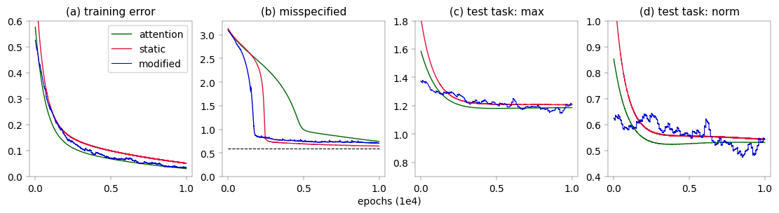
Figure 1: (a) Training error of the attention, static and modified Transformers. (b) Learning a misspecified task containing two extra features. (c) Test error for the nonlinear maximum task $\max_{1\leq j\leq k}h_{\mu^{\circ}}(\bm{x})$; (d) for the norm task $\lVert h_{\mu^{\circ}}(\bm{x})\rVert$.

5.3 Second-order Improvement

We now arrive at the main difficulty of our analysis: the behavior of mean-field dynamics near critical points. In the finite-dimensional case, local stability is determined by the Hessian matrix. We show that the mean-field analogue is

Lemma 5.4.

For a smooth functional $F:\operatorname{\mathscr{P}}_{2}(\Theta)\to\operatorname{\mathbb{R}}$, the velocity field $\nabla\frac{\delta F}{\delta\mu}$ of (1) satisfies the evolution equation

$$\textstyle\partial_{t}\left[\nabla\frac{\delta F}{\delta\mu}(\mu_{t})\right]=-\operatorname{\mathcal{H}}_{\mu_{t}}\left[\nabla\frac{\delta F}{\delta\mu}(\mu_{t})\right].$$ (7)

This is the non-perturbative or tangent curve version of Lemma 4.1. For the specific objective $\operatorname{\mathcal{L}}$, we show that $\operatorname{\mathcal{H}}_{\mu}$ is Hilbert-Schmidt and derive regularity properties in Lemma E.3 and E.5. Next, the following lemma translates second-order instability into a spectral bound for $\operatorname{\mathcal{H}}_{\mu}$.

Proposition 5.5.

Suppose MFD with birth-death at time $t$ satisfies Theorem 3.3ii with $\frac{\mathop{}\!\mathrm{d}^{2}}{\mathop{}\!\mathrm{d}s^{2}}\big{|}_{s=0}\operatorname{\mathcal{L}}(\bar{\mu}_{s})\leq-\Lambda$. Then the smallest eigenvalue $\lambda_{0}$ of $\operatorname{\mathcal{H}}_{\mu_{t}}$ satisfies $\lambda_{0}\leq-R_{4}^{-1}\gamma\Lambda$.

Therefore we expect that even if the dynamics is close to a saddle point and Proposition 5.2 is not useful, as long as the $L^{2}$-component along the eigenfunction $\psi_{0}$ corresponding to $\lambda_{0}$ is not exactly zero, it will blow up exponentially in time until $\mu_{t}$ escapes and makes progress. In detail,

Theorem 5.6.

Suppose MFD with birth-death on $\operatorname{\mathcal{L}}$ at time $t$ satisfies Theorem 3.3i with $\frac{\mathop{}\!\mathrm{d}}{\mathop{}\!\mathrm{d}s}\big{|}_{s=0}\operatorname{\mathcal{L}}(\bar{\mu}_{s})\geq-O(k^{-1}\operatorname{\mathcal{L}}(\mu_{t})^{2})$. Further suppose the eigenfunction $\psi_{0}$ satisfies $|\int\psi_{0}^{\top}\nabla\frac{\delta\!\operatorname{\mathcal{L}}}{\delta\mu}(\mu_{t})\mathop{}\!\mathrm{d}\mu_{t}|\geq\alpha$ for some $\alpha\geq 0$. Then MFD within the region $\{\mu\in\operatorname{\mathscr{P}}_{2}(\Theta):\lambda_{\textup{min}}(\bm{\Sigma}_{\mu,\mu})=\Omega(\frac{1}{k})\}$ decreases $\operatorname{\mathcal{L}}$ in time $\tau=\widetilde{O}\left(\frac{k}{\gamma\operatorname{\mathcal{L}}(\mu_{t})^{2}}\log\frac{1}{\alpha}\right)$ as

$$\textstyle\operatorname{\mathcal{L}}(\mu_{t+\tau})\leq\operatorname{\mathcal{L}}(\mu_{t})-\widetilde{\Omega}\left(\frac{\gamma^{2}\alpha\operatorname{\mathcal{L}}(\mu_{t})^{4}}{k^{5}d}\right).$$

Simply put, we make $\widetilde{O}(\alpha)$ progress in $\widetilde{O}(\log\frac{1}{\alpha})$ time. The proof idea is to find a $\operatorname{\mathcal{W}}_{2}$-ball where if $\mu_{t}$ does not escape in time $\tau$, the exponential blowup guarantees improvement of $\operatorname{\mathcal{L}}$; if $\mu_{t}$ does escape, $\operatorname{\mathcal{L}}$ must have decreased enough to warrant such movement (via the Benamou-Brenier formula). Again, we present general versions of Proposition 5.5 and Theorem 5.6 as Proposition E.6 and Theorem E.7.

Dimensional dependency.

The rate is polynomial in the number of features $k$ but only linear in $d$, mitigating the curse of dimensionality. Initially $\operatorname{\mathcal{L}}$ decreases by $\widetilde{\Omega}(k^{-5}d^{-1})$ in time $\widetilde{O}(k)$ when $\operatorname{\mathcal{L}}=\Theta(1)$. As training progresses, the rate worsens to $\widetilde{\Omega}(k^{-9}d^{-1})$ in time $\widetilde{O}(k^{3})$ when $\operatorname{\mathcal{L}}=\Theta(\frac{1}{k})$ due to the smaller curvature of $\operatorname{\mathcal{L}}$, until we enter the accelerated convergence phase and Theorem 5.3 takes over.

Since $\operatorname{\mathcal{L}}$ becomes ill-conditioned if $h_{\mu}(\bm{x})$ is nearly constrained on a subspace, we have assumed that $\lambda_{\textup{min}}(\bm{\Sigma}_{\mu,\mu})$ is locally bounded below (on the same order as the upper bound $\frac{R_{1}^{2}}{k}$) to obtain regularity estimates. We expect this to not be a problem in practice since $\mathbf{W}$ will not diverge without timescale separation. In our experiments, $\lambda_{\textup{min}}(\bm{\Sigma}_{\mu,\mu})$ never varied by over 25% during each training phase.

5.4 Escaping from Saddle Points Efficiently

Theorem 5.6 on its own cannot ensure convergence rates. The flow might be initialized at or pass near multiple saddle points with very small $\alpha$ values, taking longer to escape. This is an unavoidable problem of nonconvex gradient descent even in finite dimensions (Du et al., 2017). In contrast, it has been shown that simply adding uniform noise allows GD to escape saddle points efficiently (Ge et al., 2015; Jin et al., 2017). Here, we suggest an adaptation to WGF.

The main problem is how to apply ‘random’ perturbations in $\operatorname{\mathscr{P}}_{2}(\Omega)$. Motivated by the characterization of the tangent space (4), we propose a scheme which constructs perturbations in the velocity space using vector-valued Gaussian processes. See Definition E.8 and Algorithm 1 for details.

1. Generate a random velocity field $\bm{\xi}:\Omega\to\operatorname{\mathbb{R}}^{m}$ from a stationary Gaussian process $\operatorname{GP}(0,\mathbf{K})$ with bounded kernel $\mathbf{K}:\Omega\times\Omega\to\operatorname{\mathbb{R}}^{m\times m}$.

2. Run the pushforward dynamics $\partial_{t}\mu_{t}=\nabla\cdot(\bm{\xi}\mu_{t})$ from $\mu_{0}=\mu^{\dagger}$ for fixed time $\Delta t$.

This can bypass the dimensional dependency in Ge et al. (2015) and ensure a nonzero $\psi_{0}$-component for $\nabla\frac{\delta F}{\delta\mu}(\mu_{\Delta t})$, which is approximately normally distributed with variance $O(\Delta t)$ (Lemma E.9). Unfortunately this naive approach is not enough to ensure large $\alpha$, at least in polynomial time, since the eigenfunction $\psi_{0}$ and base measure also change along the perturbation. Jin et al. (2017) bypass this issue in finite dimensions via a geometric argument; we conjecture that our method also guarantees polynomial escape time. If this is true, we may combine Proposition 5.2 with $\delta=O(k^{-1}\operatorname{\mathcal{L}}(\mu_{t})^{2})$, yielding $O(\frac{k^{6}}{\gamma^{3}t^{3}})$ convergence away from saddle points, and Theorem 5.6 to conclude that perturbed WGF enjoys polynomial convergence to global minima.

6 Numerical Experiments

Complementing our theoretical analyses, we now explore some empirical aspects of in-context feature learning of a toy Transformer. We compare three models: the attention Transformer is constructed as in Section 2.2 and jointly optimizes the loss $\operatorname{\mathcal{L}}_{\textup{TF}}(\mu,\mathbf{W})$, while the static and modified Transformers directly minimize $\operatorname{\mathcal{L}}(\mu)$ without passing through the LSA layer. All models are pretrained using SGD on 10K prompts each containing 1K token pairs. For the MLP we set $d=20$, $k=5$ with 500 sigmoid neurons and $\operatorname{\mathcal{D}}_{\operatorname{\mathscr{X}}}\sim\mathcal{N}(0,\mathbf{I}_{d})$. The modified model additionally implements the birth-death and perturbation dynamics of Section 5 if $\operatorname{\mathcal{L}}$ has not decreased by 1% every 100 epochs.

Figure 1(a) shows that attention and static Transformers exhibit similar dynamics and successfully converge to global optima, justifying the two-timescale approach. Next, Figure 1(b) plots the training curve for a misspecified model where the true features $h_{\mu^{\circ}}$ are 7-dimensional. While zero loss is not achievable due to the increased complexity, all models still find a well-behaved minimum, and the modified dynamics escapes a potential saddle point more quickly. Finally, we compute the test loss w.r.t. two nonlinear feature-based tasks $\max_{1\leq j\leq k}h_{\mu^{\circ}}(\bm{x})_{j}$ and $\lVert h_{\mu^{\circ}}(\bm{x})\rVert$ in Figures 1(c),(d). Accuracy sharply improves when the relevant features are learned, confirming that ICFL can generalize beyond linear regression even in one-layer Transformers and further demonstrating the importance of feature learning.

7 Conclusion

In this paper, we explored the training dynamics of a Transformer with one MLP and one attention layer, enabling in-context feature learning of regression tasks on a rich class of representations. We showed that the loss landscape becomes benign in the two-timescale and mean-field limit and developed instability and improvement guarantees for the Wasserstein gradient flow. To our knowledge, this represents both the first work to theoretically study how features are learned in context, and the first analysis of nonconvex mean-field dynamics for strict saddle objectives. We hope our insights may be extended to more complex in-context learning behavior in deeper MLP-attention models.

Impact Statement

This paper aims to deepen our perception of how in-context learning ability arises in Transformer architectures, which is intimately connected to ethical issues such as AI privacy, fairness and accountability. We hope that our study will lead to a better understanding of the reasoning capabilities of large language models and facilitate the development of more responsible, transparent and socially beneficial AI systems.

Appendix A Preliminaries

We begin by providing some necessary background for mean-field dynamics. Let $\Omega\subseteq\operatorname{\mathbb{R}}^{m}$ be a Euclidean domain with smooth boundary $\partial\Omega$. For $p\geq 1$, let $\operatorname{\mathscr{P}}_{p}(\Omega)$ be the $p$-Wasserstein space of probability measures on $\Omega$ vanishing on $\partial\Omega$ with finite $p$th moment. We will mostly be concerned with the space $\operatorname{\mathscr{P}}_{2}(\Omega)$.

Definition A.1 (functional derivative).

The functional derivative $\frac{\delta F}{\delta\mu}$ of a functional $F:\operatorname{\mathscr{P}}_{p}(\Omega)\to\operatorname{\mathbb{R}}$ is defined (if one exists) as a functional $\frac{\delta F}{\delta\mu}:\operatorname{\mathscr{P}}_{p}(\Omega)\times\Omega\to\operatorname{\mathbb{R}}$ satisfying for all $\nu\in\operatorname{\mathscr{P}}_{p}(\Omega)$,

$$\frac{\mathop{}\!\mathrm{d}}{\mathop{}\!\mathrm{d}\epsilon}\bigg{|}_{\epsilon=0}F(\mu+\epsilon(\nu-\mu))=\int_{\Omega}\frac{\delta F}{\delta\mu}(\mu,\theta)(\nu-\mu)(\mathop{}\!\mathrm{d}\theta).$$

Note that the functional derivative is defined up to additive constants. We say a functional $F$ is $C^{1}$ if $\nabla\frac{\delta F}{\delta\mu}(\mu,\theta)$ is well-defined and continuous, and $C^{2}$ if $\nabla_{\theta}\nabla_{\theta^{\prime}}\frac{\delta^{2}\!F}{\delta\mu^{2}}(\mu,\theta,\theta^{\prime})$ is well-defined and continuous. Furthermore, the functional $F$ is convex if for all $\nu\in\operatorname{\mathscr{P}}_{p}(\Omega)$ it holds that

$$F(\nu)\geq F(\mu)+\int_{\Omega}\frac{\delta F}{\delta\mu}(\mu,\theta)(\nu-\mu)(\mathop{}\!\mathrm{d}\theta).$$

Definition A.2 ($p$-Wasserstein metric).

The $p$-Wasserstein distance between $\mu,\nu\in\operatorname{\mathscr{P}}_{p}(\Omega)$ is defined as

$$\operatorname{\mathcal{W}}_{p}(\mu,\nu)=\left(\inf_{\gamma\in\Pi(\mu,\nu)}\int_{\operatorname{\mathbb{R}}^{m}}\lVert x-y\rVert^{p}\mathop{}\!\mathrm{d}\gamma(x,y)\right)^{\frac{1}{p}}$$

where $\Pi(\mu,\nu)$ denotes the set of joint distributions on $\Omega\times\Omega$ whose first and second factors have marginal laws $\mu$ and $\nu$, respectively.

We consider $\operatorname{\mathscr{P}}_{p}(\Omega)$ as a metric space with respect to $\operatorname{\mathcal{W}}_{p}$, which metrizes weak convergence on $\operatorname{\mathscr{P}}_{p}(\Omega)$ (Villani, 2009, Theorem 6.9). By Hölder’s inequality it always holds that $\operatorname{\mathscr{P}}_{2}(\Omega)\subset\operatorname{\mathscr{P}}_{1}(\Omega)$ and $\operatorname{\mathcal{W}}_{1}(\mu,\nu)\leq\operatorname{\mathcal{W}}_{2}(\mu,\nu)$. The $\operatorname{\mathcal{W}}_{1}$ metric is also characterized via Kantorovich-Rubinstein duality as

$$\operatorname{\mathcal{W}}_{1}(\mu,\nu)=\sup_{\lVert f\rVert_{\operatorname{\mathrm{Lip}}}\leq 1}\int_{\Omega}f\mathop{}\!\mathrm{d}\mu-\int_{\Omega}f\mathop{}\!\mathrm{d}\nu,$$

where the supremum runs over all 1-Lipschitz functions $f:\Omega\to\operatorname{\mathbb{R}}$, which makes it well-suited for perturbation analyses.

We develop more advanced theory concerning the local metric geometry and characterization of flows on $\operatorname{\mathscr{P}}_{2}(\Omega)$ in Appendix D. As a consequence, one can show the following variational formulation of the $\operatorname{\mathcal{W}}_{2}$ metric:

Proposition A.3 (Benamou-Brenier formula).

For $\mu,\nu\in\operatorname{\mathscr{P}}_{2}(\Omega)$ it holds that

$$\operatorname{\mathcal{W}}_{2}(\mu,\nu)=\inf\left\{\int_{0}^{1}\lVert\bm{v}_{t}\rVert_{L^{2}(\Omega,\mu_{t};\operatorname{\mathbb{R}}^{m})}^{2}\mathop{}\!\mathrm{d}t:\partial_{t}\mu_{t}+\nabla\cdot(\bm{v}_{t}\mu_{t})=0,\;\mu_{0}=\mu,\,\mu_{1}=\nu\right\},$$

where the infimum runs over all unit time flows $(\mu_{t})_{t\in[0,1]}$ from $\mu$ to $\nu$.

Proof.

See e.g. Ambrosio et al. (2005), Chapter 8 or Santambrogio (2015), Section 6.1. ∎

The formula can be used to bound the movement of Wasserstein flows in relation to the magnitude of the gradient field. For convenience, we will use the following time-rescaled version which is easily checked:

$$\operatorname{\mathcal{W}}_{2}(\mu,\nu)=\inf\left\{\tau\int_{0}^{\tau}\lVert\bm{v}_{t}\rVert_{L^{2}(\Omega,\mu_{t};\operatorname{\mathbb{R}}^{m})}^{2}\mathop{}\!\mathrm{d}t:\partial_{t}\mu_{t}+\nabla\cdot(\bm{v}_{t}\mu_{t})=0,\;\mu_{0}=\mu,\,\mu_{\tau}=\nu,\,\tau>0\right\}.$$

When the velocity field $\bm{v}_{t}=-\nabla\frac{\delta F}{\delta\mu}(\mu_{t})$ is given as the functional derivative of a given functional $F$, the dynamics can be interpreted as the continuous-time limit of a discrete gradient descent process on $F$ w.r.t. the $\operatorname{\mathcal{W}}_{2}$ metric via the celebrated JKO scheme (Jordan et al., 1998). Specifically, the implicit Euler scheme

$$\mu_{\eta}^{(k+1)}=\operatorname*{arg\,min}_{\mu\in\operatorname{\mathscr{P}}_{2}(\Omega)}\frac{1}{2}\operatorname{\mathcal{W}}_{2}(\mu,\mu^{(k)})^{2}+\eta F(\mu),\quad\mu^{(0)}=\mu_{0}$$

converges weakly in the limit $\eta\to 0$ to the solution of the continuity or Fokker-Planck equation $\partial_{t}\mu_{t}=\nabla\cdot\left(\mu_{t}\nabla\frac{\delta F}{\delta\mu}(\mu_{t})\right)$ in the sense that $\mu_{\eta}^{\lfloor t/\eta\rfloor}\rightharpoonup\mu_{t}$ for all time $t\geq 0$. Hence we refer to this process as the Wasserstein gradient flow on $\operatorname{\mathscr{P}}_{2}(\Omega)$ with respect to $F$.

Implementation.

We provide a simple summary of the proposed modified mean-field dynamics in Algorithm 1. Here $\theta_{k}^{(1)},\cdots,\theta_{k}^{(N)}$ denote the values of the $N$ particles at step $k$ with empirical distribution $\widehat{\mu}_{k}=\frac{1}{N}\sum_{j=1}^{N}\delta_{\theta_{k}^{(j)}}$, $\epsilon$ is the convergence error and $\delta_{b},\delta_{p}$ are improvement thresholds for applying the birth-death and perturbation procedures, respectively. We also set learning rate $\eta$, perturbation step size $\eta_{p}$ and a waiting time $\tau$ for escaping saddle points. More generally, $\delta_{b},\delta_{p}$ could be decreased and $\tau$ could be increased depending on the current objective value as suggested in Theorem 5.6. In addition, the density ratio $\frac{\mathop{}\!\mathrm{d}\mu_{t}}{\mathop{}\!\mathrm{d}\pi}$ could be estimated at certain steps to directly check for the birth-death condition; see Sugiyama et al. (2018) for an overview of applicable methods, especially in high dimensions.

Algorithm 1 Mean-field dynamics with birth-death and perturbation

0:  i.i.d. samples $\theta_{0}^{(1)},\cdots,\theta_{0}^{(N)}\sim\mu_{0}$

  while $\operatorname{\mathcal{L}}(\widehat{\mu}_{k})>\epsilon$ do

     Update all particles as $\theta_{k+1}^{(j)}=\theta_{k}^{(j)}-\eta\nabla\frac{\delta\!\operatorname{\mathcal{L}}}{\delta\mu}(\widehat{\mu}_{k},\theta_{k}^{(j)})$, $j\in[N]$

     if $\operatorname{\mathcal{L}}(\widehat{\mu}_{k})-\operatorname{\mathcal{L}}(\widehat{\mu}_{k+1})\leq\delta_{b}$ then

        Randomly replace $\lfloor\gamma N\rfloor$ neurons with i.i.d. samples from $\pi$

     end if

     if $\operatorname{\mathcal{L}}(\widehat{\mu}_{k})-\operatorname{\mathcal{L}}(\widehat{\mu}_{k+1})\leq\delta_{p}$ and $k-k_{p}>\tau$ then

        $k_{p}\leftarrow k$

        Generate a Gaussian process $\bm{\xi}\sim\operatorname{GP}(0,\mathbf{K})$

        Update all particles as $\theta_{k+1}^{(j)}=\theta_{k}^{(j)}-\eta_{p}\nabla\bm{\xi}(\theta_{k}^{(j)})$, $j\in[N]$

     end if

     $k\leftarrow k+1$

  end while

Appendix B Proofs for Section 2

B.1 Barron Class Analysis of Representations

Lemma B.1.

For any $p>1$ it holds that $\lVert f\rVert_{\operatorname{\mathscr{B}}_{1}}=\lVert f\rVert_{\operatorname{\mathscr{B}}_{p}}=\lVert f\rVert_{\operatorname{\mathscr{B}}_{\infty}}$, where

$$\lVert f\rVert_{\operatorname{\mathscr{B}}_{\infty}}:=\inf_{\mu:f=h_{\mu}}\operatorname*{ess\,sup}_{(\bm{a},\bm{w})\sim\mu}\lVert\bm{a}\rVert\lVert\bm{w}\rVert.$$

Proof.

Note $\lVert f\rVert_{\operatorname{\mathscr{B}}_{1}}\leq\lVert f\rVert_{\operatorname{\mathscr{B}}_{p}}\leq\lVert f\rVert_{\operatorname{\mathscr{B}}_{\infty}}$ trivially by Hölder’s inequality. For $f\in\operatorname{\mathscr{B}}_{1}$, choose a measure $\mu$ such that $f=h_{\mu}$ and $\int\lVert\bm{a}\rVert\lVert\bm{w}\rVert\mu(\mathop{}\!\mathrm{d}\theta)\leq\lVert f\rVert_{\operatorname{\mathscr{B}}_{1}}+\epsilon$ and define the nonnegative measure $\underline{\mu}$ on $\mathbb{S}^{k-1}\times\mathbb{S}^{d-1}$ as

$$\underline{\mu}(A,B)=\int_{\underline{\bm{a}}\in A,\underline{\bm{w}}\in B}\lVert\bm{a}\rVert\lVert\bm{w}\rVert\mu(\mathop{}\!\mathrm{d}\bm{a},\mathop{}\!\mathrm{d}\bm{w}),\quad\underline{\bm{a}}=\frac{\bm{a}}{\lVert\bm{a}\rVert},\quad\underline{\bm{w}}=\frac{\bm{w}}{\lVert\bm{w}\rVert}$$

for Borel sets $A\subseteq\mathbb{S}^{k-1}$, $B\subseteq\mathbb{S}^{d-1}$. Then we can rewrite $f$ via the ‘projected’ measure $\underline{\mu}$ as

$$f =\int h_{\theta}(\bm{x})\mu(\mathop{}\!\mathrm{d}\theta)=\int\lVert\bm{a}\rVert\lVert\bm{w}\rVert\cdot\underline{\bm{a}}\sigma(\underline{\bm{w}}^{\top}\bm{x})\mu(\mathop{}\!\mathrm{d}\bm{a},\mathop{}\!\mathrm{d}\bm{w})=\int\underline{\bm{a}}\sigma(\underline{\bm{w}}^{\top}\bm{x})\underline{\mu}(\mathop{}\!\mathrm{d}\bm{a},\mathop{}\!\mathrm{d}\bm{w}).$$

Factoring out the total mass of $\underline{\mu}$ to form a probability distribution on $\operatorname{\mathscr{P}}(\mathbb{S}^{k-1}\times\mathbb{S}^{d-1})$, we obtain a representation of $f$ such that the $\infty$-Barron norm becomes bounded as

$$\lVert f\rVert_{\operatorname{\mathscr{B}}_{\infty}}\leq\underline{\mu}(\mathbb{S}^{k-1},\mathbb{S}^{d-1})\operatorname*{ess\,sup}_{(\bm{a},\bm{w})\sim\underline{\mu}}\lVert\bm{a}\rVert\lVert\bm{w}\rVert\leq\lVert f\rVert_{\operatorname{\mathscr{B}}_{1}}+\epsilon.$$

Taking $\epsilon\to 0$ shows the reverse inequality. ∎

Proof of Proposition 2.1.

If $f_{j}\in C(\operatorname{\mathscr{X}},\operatorname{\mathbb{R}})$ satisfies $\textstyle\inf_{\widehat{f}_{j}}\int_{\operatorname{\mathbb{R}}^{d-1}}\lVert\omega\rVert_{1}^{2}|\widehat{f}_{j}(\omega)|<\infty$ for some transform $\widehat{f}_{j}$, it admits a representation

$$f_{j}(\bm{x})=\int a_{j}\sigma(\bm{w}^{\top}\bm{x})\mu_{j}(\mathop{}\!\mathrm{d}a_{j},\mathop{}\!\mathrm{d}\bm{w})$$

for a probability distribution $\mu_{j}$ on $\operatorname{\mathbb{R}}\times\operatorname{\mathbb{R}}^{d}$ (Barron, 1993; Weinan et al., 2022). Consider the scaled inclusion map

$$\iota_{j}:\operatorname{\mathbb{R}}\times\operatorname{\mathbb{R}}^{d}\hookrightarrow\operatorname{\mathbb{R}}^{k}\times\operatorname{\mathbb{R}}^{d},\quad\iota_{j}(a_{j},\bm{w})=(ka_{j}e_{j},\bm{w}),$$

where $e_{j}$ is the unit vector with all zeros except for a single 1 at the $j$th coordinate. Then for the averaged pushforward measure $\bar{\mu}=\frac{1}{k}\sum_{j=1}^{k}\iota_{j}\sharp\mu_{j}\in\operatorname{\mathscr{P}}(\Theta)$ it holds that

$$h_{\bar{\mu}}(\bm{x})=\frac{1}{k}\sum_{j=1}^{k}\int\bm{a}_{j}\sigma(\bm{w}^{\top}\bm{x})\iota_{j}\sharp\mu_{j}(\mathop{}\!\mathrm{d}\bm{a}_{j},\mathop{}\!\mathrm{d}\bm{w})=\sum_{j=1}^{k}\int a_{j}e_{j}\sigma(\bm{w}^{\top}\bm{x})\mu_{j}(\mathop{}\!\mathrm{d}\bm{a}_{j},\mathop{}\!\mathrm{d}\bm{w})=\sum_{j=1}^{k}e_{j}f_{j}(\bm{x})=f(\bm{x}),$$

and therefore $f\in\operatorname{\mathscr{B}}$. ∎

Proof of Lemma 2.2.

Let $\mathbf{A}^{\dagger}$ denote the pseudoinverse of a matrix $\mathbf{A}$. If $f^{\circ}=h_{\mu^{\circ}}$ for some distribution $\mu^{\circ}\in\operatorname{\mathscr{P}}(\Theta)$ with $\lVert f^{\circ}\rVert_{\operatorname{\mathscr{B}}}<\infty$, then setting $\mathbf{W}^{\circ}=\bm{\Sigma}_{\mu^{\circ},\mu^{\circ}}^{\dagger}=\mathbb{E}_{\bm{x}}[f^{\circ}(\bm{x})f^{\circ}(\bm{x})^{\top}]^{\dagger}$,

$$\operatorname{\mathcal{L}}_{\textup{TF}}(\mu^{\circ},\mathbf{W}^{\circ}) =\frac{1}{2}\mathbb{E}_{\bm{x}_{\textup{qr}}}\left[\left\lVert f^{\circ}(\bm{x}_{\textup{qr}})-\bm{\Sigma}_{\mu^{\circ},\mu^{\circ}}\mathbf{W}^{\circ}f^{\circ}(\bm{x}_{\textup{qr}})\right\rVert^{2}\right]$$

$$=\frac{1}{2}\operatorname{tr}\bm{\Sigma}_{\mu^{\circ},\mu^{\circ}}-\operatorname{tr}\left(\bm{\Sigma}_{\mu^{\circ},\mu^{\circ}}\mathbf{W}^{\circ}\bm{\Sigma}_{\mu^{\circ},\mu^{\circ}}\right)+\frac{1}{2}\operatorname{tr}\left(\bm{\Sigma}_{\mu^{\circ},\mu^{\circ}}\mathbf{W}^{\circ}\bm{\Sigma}_{\mu^{\circ},\mu^{\circ}}\mathbf{W}^{\circ}\bm{\Sigma}_{\mu^{\circ},\mu^{\circ}}\right)$$

$$=0.$$

Conversely, $\operatorname{\mathcal{L}}_{\textup{TF}}(\mu,\mathbf{W})=0$ implies that $f^{\circ}(\bm{x}_{\textup{qr}})=\mathbb{E}_{\bm{x}}[f^{\circ}(\bm{x})h_{\mu}(\bm{x})^{\top}]\mathbf{W}h_{\mu}(\bm{x}_{\textup{qr}})$ or $f^{\circ}=\mathbf{A}h_{\mu}$ for some $\mathbf{A}\in\operatorname{\mathbb{R}}^{k\times k}$. Then the pushforward measure $\mathbf{A}\sharp\mu$ of $\mu$ along the map $(\bm{a},\bm{w})\mapsto(\mathbf{A}\bm{a},\bm{w})$ satisfies

$$h_{\mathbf{A}\sharp\mu}(\bm{x})=\int\mathbf{A}\bm{a}\sigma(\bm{w}^{\top}\bm{x})\mu(\mathop{}\!\mathrm{d}\theta)=\mathbf{A}h_{\mu}(\bm{x})=f^{\circ}(\bm{x}),\quad\operatorname*{ess\,sup}_{\mathbf{A}\sharp\mu}\lVert\bm{a}\rVert\lVert\bm{w}\rVert\leq\lVert\mathbf{A}\rVert\operatorname*{ess\,sup}_{\mu}\lVert\bm{a}\rVert\lVert\bm{w}\rVert<\infty,$$

thus $f^{\circ}=h_{\mathbf{A}\sharp\mu}\in\operatorname{\mathscr{B}}$. ∎

Proof of Proposition 2.3.

Since the minimization problem is standard linear regression, we can explicitly set

$$\bm{v}=\mathbb{E}_{\bm{x}}[f^{\circ}(\bm{x})f^{\circ}(\bm{x})^{\top}]^{\dagger}\mathbb{E}_{\bm{x}}[g(\bm{x})f^{\circ}(\bm{x})],\quad\lVert\bm{v}\rVert\leq\lVert\mathbb{E}_{\bm{x}}[f^{\circ}(\bm{x})f^{\circ}(\bm{x})^{\top}]^{\dagger}\rVert\cdot\lVert f^{\circ}\rVert_{L^{2}(\operatorname{\mathcal{D}}_{\operatorname{\mathscr{X}}})}\lVert g\rVert_{L^{2}(\operatorname{\mathcal{D}}_{\operatorname{\mathscr{X}}})}.$$

Writing $g_{0}=g-\bm{v}^{\top}f^{\circ}$, we can bound

$$\frac{1}{2}\mathbb{E}_{\bm{x}_{\textup{qr}}}\left[\left\lVert g(\bm{x}_{\textup{qr}})-\mathbb{E}_{\bm{x}}[g(\bm{x})h_{\mu}(\bm{x})^{\top}]\mathbf{W}h_{\mu}(\bm{x}_{\textup{qr}})\right\rVert^{2}\right]$$

$$\leq\lVert\bm{v}\rVert^{2}\mathbb{E}_{\bm{x}_{\textup{qr}}}\left[\left\lVert f^{\circ}(\bm{x}_{\textup{qr}})-\mathbb{E}_{\bm{x}}[f^{\circ}(\bm{x})h_{\mu}(\bm{x})^{\top}]\mathbf{W}h_{\mu}(\bm{x}_{\textup{qr}})\right\rVert^{2}\right]+\mathbb{E}_{\bm{x}_{\textup{qr}}}\left[\left\lVert g_{0}(\bm{x}_{\textup{qr}})-\mathbb{E}_{\bm{x}}[g_{0}(\bm{x})h_{\mu}(\bm{x})^{\top}]\mathbf{W}h_{\mu}(\bm{x}_{\textup{qr}})\right\rVert^{2}\right]$$

$$\leq 2\lVert\bm{v}\rVert^{2}\epsilon+2\lVert g_{0}\rVert_{L^{2}(\operatorname{\mathcal{D}}_{\operatorname{\mathscr{X}}})}^{2}+2\lVert g_{0}\rVert_{L^{2}(\operatorname{\mathcal{D}}_{\operatorname{\mathscr{X}}})}^{2}\lVert h_{\mu}\rVert_{L^{2}(\operatorname{\mathcal{D}}_{\operatorname{\mathscr{X}}})}^{4}\lVert\mathbf{W}\rVert^{2}.$$

The statement follows by noting that

$$\lVert h_{\mu}\rVert_{L^{2}(\operatorname{\mathcal{D}}_{\operatorname{\mathscr{X}}})}\leq\left(\int\mathbb{E}_{\bm{x}}[\lVert h_{\theta}(\bm{x})\rVert^{2}]\mu(\mathop{}\!\mathrm{d}\theta)\right)^{1/2}\leq\left(\int\lVert\bm{a}\rVert^{2}\lVert\bm{w}\rVert^{2}\mathbb{E}_{\bm{x}}[\lVert\bm{x}\rVert^{2}]\mu(\mathop{}\!\mathrm{d}\theta)\right)^{1/2}=M_{2}^{1/2}\lVert h_{\mu}\rVert_{\operatorname{\mathscr{B}}}$$

from the limiting argument in Lemma B.1. ∎

B.2 Finite-width Approximation and Optimization

Proof of Proposition 2.4.

For any network $\mu$, we may take $\mathbf{W}=\mathbb{E}_{\bm{x}}[f^{\circ}(\bm{x})h_{\mu}(\bm{x})^{\top}]^{\dagger}$ so that

$$\inf_{\mathbf{W}}\operatorname{\mathcal{L}}_{\textup{TF}}(\mu,\mathbf{W}) \leq\frac{1}{2}\mathbb{E}_{\bm{x}_{\textup{qr}}}\left[\left\lVert f^{\circ}(\bm{x}_{\textup{qr}})-\mathbb{E}_{\bm{x}}[f^{\circ}(\bm{x})h_{\mu}(\bm{x})^{\top}]\mathbf{W}h_{\mu}(\bm{x}_{\textup{qr}})\right\rVert^{2}\right]$$

$$=\frac{1}{2}\mathbb{E}_{\bm{x}}[\lVert f^{\circ}(\bm{x})\rVert^{2}]-\operatorname{tr}\left(\mathbb{E}_{\bm{x}}[f^{\circ}(\bm{x})h_{\mu}(\bm{x})^{\top}]\mathbf{W}\mathbb{E}_{\bm{x}}[h_{\mu}(\bm{x})f^{\circ}(\bm{x})^{\top}]\right)$$

$$\qquad+\frac{1}{2}\operatorname{tr}\left(\mathbf{W}^{\top}\mathbb{E}_{\bm{x}}[h_{\mu}(\bm{x})f^{\circ}(\bm{x})^{\top}]\mathbb{E}_{\bm{x}}[f^{\circ}(\bm{x})h_{\mu}(\bm{x})^{\top}]\mathbf{W}\bm{\Sigma}_{\mu,\mu}\right)$$

$$\leq\frac{1}{2}\mathbb{E}_{\bm{x}}[\lVert f^{\circ}(\bm{x})\rVert^{2}]-\operatorname{tr}\left(\mathbb{E}_{\bm{x}}[f^{\circ}(\bm{x})h_{\mu}(\bm{x})^{\top}]\right)+\frac{1}{2}\operatorname{tr}\bm{\Sigma}_{\mu,\mu}$$

$$=\frac{1}{2}\mathbb{E}_{\bm{x}}[\lVert f^{\circ}(\bm{x})-h_{\mu}(\bm{x})\rVert^{2}].$$

Now let $\mu^{\circ}\in\operatorname{\mathscr{P}}(\Theta)$ be a distribution such that $f^{\circ}=h_{\mu^{\circ}}$ and $\int\lVert\bm{a}\rVert^{2}\lVert\bm{w}\rVert^{2}\mu^{\circ}(\mathop{}\!\mathrm{d}\theta)\leq(1+\epsilon)\lVert f^{\circ}\rVert_{\operatorname{\mathscr{B}}}^{2}$. Let $\theta^{(1)},\cdots,\theta^{(N)}$ be an i.i.d. sample from $\mu^{\circ}$. Then from $\mathbb{E}_{\theta\sim\mu^{\circ}}[h_{\theta}(\bm{x})]=h_{\mu^{\circ}}(\bm{x})$, it holds on average that

$$\mathbb{E}_{\widehat{\mu}_{N}}\mathbb{E}_{\bm{x}}[\lVert\widehat{h}_{N}(\bm{x})-f^{\circ}(\bm{x})\rVert^{2}]$$

$$=\mathbb{E}_{\bm{x}}\mathbb{E}_{\widehat{\mu}_{N}}\left[\Bigg{\lVert}\frac{1}{N}\sum_{j=1}^{N}h_{\theta^{(j)}}(\bm{x})-f^{\circ}(\bm{x})\Bigg{\rVert}^{2}\right]$$

$$=\frac{1}{N^{2}}\sum_{j=1}^{N}\mathbb{E}_{\bm{x}}\mathbb{E}_{\widehat{\mu}_{N}}\left[\lVert h_{\theta^{(j)}}(\bm{x})-h_{\mu^{\circ}}(\bm{x})\rVert^{2}\right]+\frac{1}{N^{2}}\sum_{j\neq\ell}\mathbb{E}_{\bm{x}}\mathbb{E}_{\widehat{\mu}_{N}}\left[(h_{\theta^{(j)}}(\bm{x})-h_{\mu^{\circ}}(\bm{x}))^{\top}(h_{\theta^{(\ell)}}(\bm{x})-h_{\mu^{\circ}}(\bm{x}))\right]$$

$$\leq\frac{1}{N^{2}}\sum_{j=1}^{N}\mathbb{E}_{\bm{x}}\mathbb{E}_{\theta^{(j)}\sim\mu^{\circ}}[\lVert h_{\theta^{(j)}}(\bm{x})\rVert^{2}]$$

$$\leq\frac{1}{N}\int\lVert\bm{a}\rVert^{2}\mathbb{E}_{\bm{x}}[(\bm{w}^{\top}\bm{x})^{2}]\mu^{\circ}(\mathop{}\!\mathrm{d}\theta)$$

$$\leq\frac{(1+\epsilon)M_{2}}{N}\lVert f^{\circ}\rVert_{\operatorname{\mathscr{B}}}^{2}.$$

Moreover, the path norm is bounded on average as $\mathbb{E}_{\widehat{\mu}_{N}}[\lVert\widehat{h}_{N}\rVert_{\mathcal{P}}]\leq(1+\epsilon)\lVert f^{\circ}\rVert_{\operatorname{\mathscr{B}}}$. Then by Markov’s inequality, the event $\lVert\widehat{h}_{N}-f^{\circ}\rVert_{L^{2}(\operatorname{\mathcal{D}}_{\operatorname{\mathscr{X}}})}^{2}>\frac{2M_{2}\lVert f^{\circ}\rVert_{\operatorname{\mathscr{B}}}^{2}}{N}$ has probability at most $\frac{1+\epsilon}{2}$, and the event $\lVert\widehat{h}_{N}\rVert_{\mathcal{P}}>3\lVert f^{\circ}\rVert_{\operatorname{\mathscr{B}}}$ has probability at most $\frac{1+\epsilon}{3}$. Hence the stated bounds hold with positive probability as $\epsilon\to 0$, thus for some size $N$ network $\widehat{\mu}_{N}$. ∎

For the propagation of chaos result, we require the following bounds.

Lemma B.2.

The second moment $m_{2}(\mu_{t})=\int\lVert\theta\rVert^{2}\mu_{t}(\mathop{}\!\mathrm{d}\theta)$ satisfies $m_{2}(\mu_{t})\leq e^{2L_{1}^{2}}m_{2}(\mu_{0})$.

Proof.

The assertion follows immediately from

$$\frac{\mathop{}\!\mathrm{d}}{\mathop{}\!\mathrm{d}t}m_{2}(\mu_{t})=\int\lVert\theta\rVert^{2}\partial_{t}\mu_{t}(\mathop{}\!\mathrm{d}\theta)=-2\int\theta^{\top}\nabla\frac{\delta F}{\delta\mu}(\mu_{t},\theta)\mu_{t}(\mathop{}\!\mathrm{d}\theta)\leq 2L_{1}^{2}m_{2}(\mu_{t}).$$

∎

Lemma B.3.

Let $\mu\in\operatorname{\mathscr{P}}_{2}(\Omega)$ and $\theta^{(1)},\cdots,\theta^{(N)}$ be an i.i.d. sample from $\mu$ with corresponding empirical distribution $\widehat{\mu}_{N}=\frac{1}{N}\sum_{j=1}^{N}\delta_{\theta^{(j)}}$. Then for dimension $m\geq 3$ it holds that $\mathbb{E}[\operatorname{\mathcal{W}}_{1}(\mu,\widehat{\mu}_{N})]\leq C_{m}\cdot m_{2}(\mu)^{1/2}N^{-1/m}$. The rate is replaced by $N^{-1/2}\log N$ if $m=2$ and $N^{-1/2}$ if $m=1$.

Proof.

See e.g. Fournier & Guillin (2015) for the case $m\geq 2$ and Bobkov & Ledoux (2019) for $m=1$. ∎

Proof of Proposition 2.5.

Consider the coupled process

$$\frac{\mathop{}\!\mathrm{d}}{\mathop{}\!\mathrm{d}t}\tilde{\theta}_{t}^{(j)}=-\nabla\frac{\delta F}{\delta\mu}(\mu_{t},\tilde{\theta}_{t}^{(j)}),\quad\tilde{\theta}_{0}^{(j)}=\theta_{0}^{(j)},\quad j\in[N]$$

and write the corresponding empirical distribution as $\tilde{\mu}_{t,N}=\frac{1}{N}\sum_{j=1}^{N}\delta_{\tilde{\theta}_{t}^{(j)}}$. For any finite time horizon $T\geq 0$, it holds that

$$\frac{1}{N}\sum_{j=1}^{N}\lVert\theta_{T}^{(j)}-\tilde{\theta}_{T}^{(j)}\rVert =\frac{1}{N}\sum_{j=1}^{N}\left\lVert\int_{0}^{T}\nabla\frac{\delta F}{\delta\mu}(\widehat{\mu}_{t,N},\theta_{t}^{(j)})-\nabla\frac{\delta F}{\delta\mu}(\mu_{t},\tilde{\theta}_{t}^{(j)})\mathop{}\!\mathrm{d}t\right\rVert$$

$$\leq\int_{0}^{T}\frac{L_{2}}{N}\sum_{j=1}^{N}\lVert\theta_{t}^{(j)}-\tilde{\theta}_{t}^{(j)}\rVert+L_{3}\operatorname{\mathcal{W}}_{1}(\widehat{\mu}_{t,N},\mu_{t})\mathop{}\!\mathrm{d}t.$$

Then applying Gronwall’s inequality and taking the expectation over random initialization, we have for all $t\in[0,T]$

$$\mathbb{E}[\operatorname{\mathcal{W}}_{1}(\widehat{\mu}_{t,N},\tilde{\mu}_{t,N})]\leq\mathbb{E}\Bigg{[}\frac{1}{N}\sum_{j=1}^{N}\lVert\theta_{t}^{(j)}-\tilde{\theta}_{t}^{(j)}\rVert\Bigg{]}\leq L_{3}e^{L_{2}T}\int_{0}^{t}\mathbb{E}[\operatorname{\mathcal{W}}_{1}(\widehat{\mu}_{s,N},\mu_{s})]\mathop{}\!\mathrm{d}s.$$

Since each trajectory $\tilde{\theta}_{t}^{(j)}$ of the coupled process is an independent sample from the true distribution $\mu_{t}$, by Lemma B.2 and B.3 it moreover holds that

$$\mathbb{E}[\operatorname{\mathcal{W}}_{1}(\widehat{\mu}_{t,N},\mu_{t})] \leq\mathbb{E}[\operatorname{\mathcal{W}}_{1}(\widehat{\mu}_{t,N},\tilde{\mu}_{t,N})]+\mathbb{E}[\operatorname{\mathcal{W}}_{1}(\tilde{\mu}_{t,N},\mu_{t})]$$

$$\leq L_{3}e^{L_{2}T}\int_{0}^{t}\mathbb{E}[\operatorname{\mathcal{W}}_{1}(\widehat{\mu}_{s,N},\mu_{s})]\mathop{}\!\mathrm{d}s+C_{m}e^{L_{1}^{2}}m_{2}(\mu_{0})^{1/2}N^{-1/m}$$

with the appropriate modification when $m=1,2$. Hence another application of Gronwall’s inequality yields

$$\mathbb{E}[\operatorname{\mathcal{W}}_{1}(\widehat{\mu}_{t,N},\mu_{t})]\leq C_{m}m_{2}(\mu_{0})^{1/2}N^{-1/m}\exp(L_{1}^{2}+L_{3}Te^{L_{2}T})\to 0$$

as $N\to\infty$. The convergence is uniform for any finite horizon $T$. ∎

Remark B.4.

When $F=\operatorname{\mathcal{L}}$, we rely on the Lipschitz constants obtained in Lemma E.4 to obtain the same statement, with the caveat that the flow must not reach the singular set $\operatorname{\mathscr{P}}_{2}^{0}(\Theta)$ in order to ensure existence and regularity of the flow; this will be a recurring issue. The result is clearly still valid for mean-field dynamics incorporating birth-death by the ordinary law of large numbers, assuming the update happens at the same instant for $\widehat{\mu}_{t}$ and $\mu_{t}$. See also Rotskoff et al. (2019) for a more involved study of birth-death dynamics.

Remark B.5.

The above bounds are not optimized; compare for example Berthier et al. (2023). Explicit uniform-in-time propagation of chaos bounds have recently been proved for convex mean-field Langevin dynamics (Chen et al., 2022; Suzuki et al., 2023) and convex-concave descent-ascent dynamics (Kim et al., 2024). It remains an open problem to prove such results for general nonconvex mean-field dynamics, with or without the entropic regularization framework.

Appendix C Proofs for Section 3

C.1 Auxiliary Results

We will use the following elementary results from linear algebra without proof.

Lemma C.1.

The spectral norm of a block matrix $\mathbf{A}=\begin{bmatrix}\mathbf{A}_{1,1}&\mathbf{A}_{1,2}\\ \mathbf{A}_{2,1}&\mathbf{A}_{2,2}\end{bmatrix}$ is bounded as $\lVert\mathbf{A}\rVert\leq\sum_{i,j=1}^{2}\lVert\mathbf{A}_{i,j}\rVert$.

Lemma C.2.

The spectral and nuclear norms are dual: $\lVert\mathbf{A}\rVert_{*}=\max_{\lVert\mathbf{B}\rVert\leq 1}\langle\mathbf{A},\mathbf{B}\rangle$ and $\lVert\mathbf{A}\rVert=\max_{\lVert\mathbf{B}\rVert_{*}\leq 1}\langle\mathbf{A},\mathbf{B}\rangle$ for any $\mathbf{A}\in\operatorname{\mathbb{R}}^{m\times m}$, $m\geq 1$. In particular, $\operatorname{tr}(\mathbf{A}^{\top}\mathbf{B})\leq\lVert\mathbf{A}\rVert\lVert\mathbf{B}\rVert_{*}$ for any $\mathbf{A},\mathbf{B}\in\operatorname{\mathbb{R}}^{m\times m}$.

Lemma C.3.

For a positive semi-definite matrix $\mathbf{A}\in\operatorname{\mathbb{R}}^{k\times k}$ it holds that $\frac{1}{k}(\operatorname{tr}\mathbf{A})^{2}\leq\operatorname{tr}\mathbf{A}^{2}\leq(\operatorname{tr}\mathbf{A})^{2}$.

The neural network output is continuous and well-behaved in the following sense:

Lemma C.4.

The map $\theta\mapsto h_{\theta}(\bm{x})$ on $\Theta$ is $(R_{1}^{2}+R_{2}^{2}\lVert\bm{x}\rVert^{2})^{1/2}$-Lipschitz for each $\bm{x}\in\operatorname{\mathscr{X}}$. Also, the map $\mu\mapsto h_{\mu}(\bm{x})$ on $\operatorname{\mathscr{P}}_{2}(\Theta)$ is $(kR_{1}^{2}+kR_{2}^{2}\lVert\bm{x}\rVert^{2})^{1/2}$-Lipschitz w.r.t. 1-Wasserstein distance for each $\bm{x}\in\operatorname{\mathscr{X}}$.

Proof.

For $\theta_{1}=(\bm{a}_{1},\bm{w}_{1}),\theta_{2}=(\bm{a}_{2},\bm{w}_{2})$ we have

$$\lVert h_{\theta_{1}}(\bm{x})-h_{\theta_{2}}(\bm{x})\rVert =\lVert\bm{a}_{1}\sigma(\bm{w}_{1}^{\top}\bm{x})-\bm{a}_{2}\sigma(\bm{w}_{2}^{\top}\bm{x})\rVert$$

$$\leq\lVert\bm{a}_{1}-\bm{a}_{2}\rVert\cdot|\sigma(\bm{w}_{1}^{\top}\bm{x})|+\lVert\bm{a}_{2}\rVert\cdot|\sigma(\bm{w}_{1}^{\top}\bm{x})-\sigma(\bm{w}_{2}^{\top}\bm{x})|$$

$$\leq R_{1}\lVert\bm{a}_{1}-\bm{a}_{2}\rVert+R_{2}\lVert\bm{w}_{1}-\bm{w}_{2}\rVert\cdot\lVert\bm{x}\rVert$$

$$\leq(R_{1}^{2}+R_{2}^{2}\lVert\bm{x}\rVert^{2})^{1/2}\lVert\theta_{1}-\theta_{2}\rVert.$$

The difference of each coordinate $|h_{\theta_{1}}(\bm{x})_{j}-h_{\theta_{2}}(\bm{x})_{j}|$ satisfies the same bound for $1\leq j\leq k$, implying that

$$|h_{\mu}(\bm{x})_{j}-h_{\nu}(\bm{x})_{j}|=\left\lvert\int_{\Theta}h_{\theta}(\bm{x})_{j}\mu(\mathop{}\!\mathrm{d}\theta)-\int_{\Theta}h_{\theta}(\bm{x})_{j}\nu(\mathop{}\!\mathrm{d}\theta)\right\rvert\leq(R_{1}^{2}+R_{2}^{2}\lVert\bm{x}\rVert^{2})^{1/2}\operatorname{\mathcal{W}}_{1}(\mu,\nu)$$

and hence $\lVert h_{\mu}(\bm{x})-h_{\nu}(\bm{x})\rVert\leq(kR_{1}^{2}+kR_{2}^{2}\lVert\bm{x}\rVert^{2})^{1/2}\operatorname{\mathcal{W}}_{1}(\mu,\nu)$. ∎

Proof of Lemma 3.1.

The gradient flow equation for $\mathbf{W}$ is given as

$$\frac{\mathop{}\!\mathrm{d}}{\mathop{}\!\mathrm{d}t}\mathbf{W}_{t} =-\frac{1}{2}\nabla_{\mathbf{W}}\operatorname{tr}\left(-2\bm{\Sigma}_{\mu^{\circ},\mu}\mathbf{W}\bm{\Sigma}_{\mu,\mu^{\circ}}+\bm{\Sigma}_{\mu^{\circ},\mu}\mathbf{W}\bm{\Sigma}_{\mu,\mu}\mathbf{W}^{\top}\bm{\Sigma}_{\mu,\mu^{\circ}}\right)$$

$$=-\bm{\Sigma}_{\mu,\mu^{\circ}}\bm{\Sigma}_{\mu^{\circ},\mu}(\mathbf{W}_{t}\bm{\Sigma}_{\mu,\mu}-\mathbf{I}_{k}).$$

Denote the singular value decomposition of $\bm{\Sigma}_{\mu,\mu^{\circ}}$ as $\mathbf{U}_{1}\mathbf{D}_{1}\mathbf{V}_{1}^{\top}$ and the spectral decomposition of $\bm{\Sigma}_{\mu,\mu}$ as $\mathbf{U}_{2}\mathbf{D}_{2}\mathbf{U}_{2}^{\top}$ where $\mathbf{U}_{1},\mathbf{U}_{2},\mathbf{V}_{1}\in\mathcal{O}(k)$ and $\mathbf{D}_{j}=\operatorname{diag}(d_{j,1},\cdots,d_{j,k})$. Since we assume $\bm{\Sigma}_{\mu,\mu}=\mathbb{E}_{\bm{x}}[h_{\mu}(\bm{x})h_{\mu}(\bm{x})^{\top}]$ is positive definite, we also have $b_{2,i}>0$ for all $i$. Further defining the auxiliary matrix $\mathbf{Z}_{t}=\mathbf{U}_{1}^{\top}\mathbf{W}_{t}\mathbf{U}_{2}$, the dynamics for $\mathbf{Z}_{t}$ is expressed as

$$\frac{\mathop{}\!\mathrm{d}}{\mathop{}\!\mathrm{d}t}\mathbf{Z}_{t} =-\mathbf{U}_{1}^{\top}(\mathbf{U}_{1}\mathbf{D}_{1}\mathbf{V}_{1}^{\top})(\mathbf{V}_{1}\mathbf{D}_{1}\mathbf{U}_{1}^{\top})(\mathbf{U}_{1}\mathbf{Z}_{t}\mathbf{D}_{2}\mathbf{U}_{2}^{\top}-\mathbf{I}_{k})\mathbf{U}_{2}$$

$$=-\mathbf{D}_{1}^{2}\mathbf{Z}_{t}\mathbf{D}_{2}+\mathbf{D}_{1}^{2}\mathbf{U}_{1}^{\top}\mathbf{U}_{2}.$$

Writing $\mathbf{U}_{1}^{\top}\mathbf{U}_{2}=(u_{i,j})_{1\leq i,j\leq k}$, for each entry $z_{i,j}(t):=(\mathbf{Z}_{t})_{i,j}$ we obtain that $z_{i,j}^{\prime}(t)=-d_{1,i}^{2}(d_{2,j}z_{i,j}(t)-u_{i,j})$ and therefore

$$\lim_{t\to\infty}z_{i,j}(t)=\begin{rcases}\begin{dcases}d_{2,j}^{-1}u_{i,j}&d_{1,i}\neq 0\\ z_{i,j}(0)&d_{1,i}=0\end{dcases}\end{rcases}=\mathbf{1}_{\{d_{1,i}\neq 0\}}d_{2,j}^{-1}u_{i,j}+\mathbf{1}_{\{d_{1,i}=0\}}z_{i,j}(0).$$

This can be recast in matrix form as $\lim_{t\to\infty}\!\mathbf{Z}_{t}=\mathbf{D}_{1}^{\dagger}\mathbf{D}_{1}\mathbf{U}_{1}^{\top}\mathbf{U}_{2}\mathbf{D}_{2}^{-1}+(\mathbf{I}_{k}-\mathbf{D}_{1}^{\dagger}\mathbf{D}_{1})\mathbf{Z}_{0}$, and the convergence rate is exponential. We conclude for the limit $\mathbf{W}_{\mu}:=\lim_{t\to\infty}\mathbf{W}_{t}$ that

$$\bm{\Sigma}_{\mu^{\circ},\mu}\mathbf{W}_{\mu}=(\mathbf{V}_{1}\mathbf{D}_{1}\mathbf{U}_{1}^{\top})\mathbf{U}_{1}\big{(}\mathbf{D}_{1}^{\dagger}\mathbf{D}_{1}\mathbf{U}_{1}^{\top}\mathbf{U}_{2}\mathbf{D}_{2}^{-1}+(\mathbf{I}_{k}-\mathbf{D}_{1}^{\dagger}\mathbf{D}_{1})\mathbf{Z}_{0}\big{)}\mathbf{U}_{2}^{\top}=(\mathbf{V}_{1}\mathbf{D}_{1}\mathbf{U}_{1}^{\top})(\mathbf{U}_{2}\mathbf{D}_{2}^{-1}\mathbf{U}_{2}^{\top})=\bm{\Sigma}_{\mu^{\circ},\mu}\bm{\Sigma}_{\mu,\mu}^{-1}.$$

∎

Proposition C.5.

For any $\mu\in\operatorname{\mathscr{P}}_{2}(\Theta)$, $\nu\in\operatorname{\mathscr{P}}_{2}^{+}(\Theta)$, there are at most $k$ values $t\in[0,1]$ such that $(1-t)\mu+t\nu\in\operatorname{\mathscr{P}}_{2}^{0}(\Theta)$. Consequently, $\operatorname{\mathscr{P}}_{2}^{+}(\Theta)$ is dense in $\operatorname{\mathscr{P}}_{2}(\Theta)$.

Note in particular that $\mathbf{R}\sharp\mu^{\circ}\in\operatorname{\mathscr{P}}_{2}^{+}(\Theta)$ for any invertible $\mathbf{R}\in\operatorname{\mathcal{B}}_{1}(k)$ as $\bm{\Sigma}_{\mathbf{R}\sharp\mu^{\circ},\mathbf{R}\sharp\mu^{\circ}}=r^{\circ}\mathbf{R}\mathbf{R}^{\top}$. This justifies the computations which appear in the statement and proof of Theorem 3.3.

Proof.

Suppose there exist $k+1$ distinct $t_{j}\in[0,1]$, $j=0,1,\cdots,k$ such that $(1-t_{j})\mu+t_{j}\nu\in\operatorname{\mathscr{P}}_{2}^{0}(\Theta)$; note that $t_{j}\neq 1$ since $\nu\in\operatorname{\mathscr{P}}_{2}^{+}(\Theta)$. Then there exist nonzero vectors $\bm{z}_{j}$ such that $(1-t_{j})\bm{z}_{j}^{\top}h_{\mu}(\bm{x})+t_{j}\bm{z}_{j}^{\top}h_{\nu}(\bm{x})\equiv 0$, and which must be linearly dependent. Without loss of generality, let $\{\bm{z}_{j}\}_{j=0}^{\ell}$ be a minimally dependent subset of $\{\bm{z}_{j}\}_{j=0}^{k}$ so that $\sum_{j=0}^{\ell}b_{j}\bm{z}_{j}=0$ for constants $b_{j}$ not all zero. Suppose $b_{0}\neq 0$. Then the equality

$$0\equiv\sum_{j=0}^{\ell}b_{j}\bm{z}_{j}^{\top}h_{\mu}(\bm{x})+\frac{t_{j}b_{j}}{1-t_{j}}\bm{z}_{j}^{\top}h_{\nu}(\bm{x})=\bigg{(}\sum_{j=0}^{\ell}\frac{t_{j}b_{j}}{1-t_{j}}\bm{z}_{j}^{\top}\bigg{)}h_{\nu}(\bm{x})$$

implies that

$$\sum_{j=0}^{\ell-1}\bigg{(}\frac{t_{j}}{1-t_{j}}-\frac{t_{\ell}}{1-t_{\ell}}\bigg{)}b_{j}\bm{z}_{j}=\sum_{j=0}^{\ell}\frac{t_{j}b_{j}}{1-t_{j}}\bm{z}_{j}-\frac{t_{\ell}}{1-t_{\ell}}\sum_{j=0}^{\ell}b_{j}\bm{z}_{j}=0,$$

which contradicts the minimality of $\{\bm{z}_{j}\}_{j=0}^{\ell}$ since the coefficient of $\bm{z}_{0}$ is nonzero. This proves the first claim. Denseness of $\operatorname{\mathscr{P}}_{2}^{+}(\Theta)$ immediately follows: for any $\mu\in\operatorname{\mathscr{P}}_{2}(\Theta)$, all but finitely many mixture distributions $(1-t)\mu+t\mu^{\circ}$ lie in $\operatorname{\mathscr{P}}_{2}^{+}(\Theta)$, so there exists a subsequence weakly converging to $\mu$ in $\operatorname{\mathscr{P}}_{2}^{+}(\Theta)$. ∎

Lemma C.6.

Any element $\mathbf{R}\in\operatorname{\mathcal{B}}_{1}(k)$ can be expressed as a convex combination of finitely many elements $\mathbf{R}_{1},\cdots,\mathbf{R}_{m}$ of $\mathcal{O}(k)$. In particular, the pushforward can be defined for any $\mathbf{R}\in\operatorname{\mathcal{B}}_{1}(k)$.

Proof.

Denote the singular value decomposition of $\mathbf{R}$ as $\mathbf{U}\mathbf{D}\mathbf{V}^{\top}$ and denote by $\mathbf{D}_{1},\cdots,\mathbf{D}_{2^{k}}$ all diagonal matrices with every diagonal element equal to $\pm 1$. Since every diagonal element of $\mathbf{D}$ has absolute value at most $1$, $\mathbf{D}$ is contained in the convex hull of $\mathbf{D}_{1},\cdots,\mathbf{D}_{2^{k}}$ and hence $\mathbf{R}$ can be written a convex combination of $\mathbf{U}\mathbf{D}_{1}\mathbf{V}^{\top},\cdots,\mathbf{U}\mathbf{D}_{2^{k}}\mathbf{V}^{\top}\in\mathcal{O}(k)$.

Furthermore, writing $\mathbf{R}=\sum_{j=1}^{m}\alpha_{j}\mathbf{R}_{j}$ for $\alpha_{j}\in(0,1)$, $\sum_{j=1}^{m}\alpha_{j}=1$ we may define for all $\mu\in\operatorname{\mathscr{P}}_{2}(\Theta)$ the pushforward measure $\mathbf{R}\sharp\mu:=\sum_{j=1}^{m}\alpha_{j}\mathbf{R}_{j}\sharp\mu$ so that

$$h_{\mathbf{R}\sharp\mu}(\bm{x})=\int_{\Theta}h_{\theta}(\bm{x})\mathop{}\!\mathrm{d}\mathbf{R}\sharp\mu(\theta)=\sum_{j=1}^{m}\alpha_{j}\int_{\Theta}h_{\theta}(\bm{x})\mathop{}\!\mathrm{d}\mathbf{R}_{j}\sharp\mu(\theta)=\sum_{j=1}^{m}\alpha_{j}\int_{\Theta}\mathbf{R}_{j}h_{\theta}(\bm{x})\mathop{}\!\mathrm{d}\mu(\theta)=\mathbf{R}h_{\mu}(\bm{x}).$$

We remark that simply defining $\mathbf{R}\sharp\mu$ as the pushforward along the map $\mathbf{R}:(\bm{a},\bm{w})\mapsto(\mathbf{R}\bm{a},\bm{w})$ would not preserve the bounded density condition (Assumption 3) for pushforwards of $\mu^{\circ}$. ∎

Proof of Lemma 3.2.

It is straightforward to check that

$$\operatorname{\mathcal{L}}(\mathbf{R}\sharp\mu^{\circ})=\frac{1}{2}\mathbb{E}_{\bm{x}}\left[\lVert h_{\mu^{\circ}}(\bm{x})-(\bm{\Sigma}_{\mu^{\circ},\mu^{\circ}}\mathbf{R}^{\top})(\mathbf{R}\bm{\Sigma}_{\mu^{\circ},\mu^{\circ}}\mathbf{R}^{\top})^{-1}\mathbf{R}h_{\mu^{\circ}}(\bm{x})\rVert^{2}\right]=0.$$

Conversely, $\operatorname{\mathcal{L}}(\mu)=0$ implies that $h_{\mu^{\circ}}(\bm{x})=\bm{\Sigma}_{\mu^{\circ},\mu}\bm{\Sigma}_{\mu,\mu}^{-1}h_{\mu}(\bm{x})$ a.e. Since $\bm{x}\mapsto h_{\mu}(\bm{x})$ is always continuous, equality holds for all $\bm{x}\in\operatorname{\mathscr{X}}$. Finally, $\bm{\Sigma}_{\mu^{\circ},\mu}\bm{\Sigma}_{\mu,\mu}^{-1}$ cannot be singular since the image of $h_{\mu^{\circ}}$ is not constrained on a lower-dimensional subspace by Assumption 2. ∎

C.2 Proof of Theorem 3.3

We study the first- and second-order properties of the optimization landscape for the functional $\operatorname{\mathcal{L}}$. Let us denote

$$\mathbf{L}_{\mu}=\frac{1}{2}\mathbb{E}_{\bm{x}}\left[\zeta_{\mu^{\circ},\mu}(\bm{x})\zeta_{\mu^{\circ},\mu}(\bm{x})^{\top}\right]=\frac{1}{2}r^{\circ}\mathbf{I}_{k}-\frac{1}{2}\bm{\Sigma}_{\mu^{\circ},\mu}\bm{\Sigma}_{\mu,\mu}^{-1}\bm{\Sigma}_{\mu,\mu^{\circ}}$$

so that $\mathbf{L}_{\mu}$ is positive semi-definite and $\operatorname{tr}\mathbf{L}_{\mu}=\operatorname{\mathcal{L}}(\mu)$. Let $\mathbf{R}\in\operatorname{\mathcal{B}}_{1}(k)$ and $\bar{\mu}_{s}=(1-s)\mu+s\mathbf{R}\sharp\mu^{\circ}$ for $s\in[0,1]$. By linearity of the mean-field mapping $\mu\mapsto h_{\mu}$,

$$\frac{\mathop{}\!\mathrm{d}}{\mathop{}\!\mathrm{d}s}h_{\bar{\mu}_{s}}(\bm{x})=\mathbf{R}h_{\mu^{\circ}}(\bm{x})-h_{\mu}(\bm{x}),\quad\frac{\mathop{}\!\mathrm{d}}{\mathop{}\!\mathrm{d}s}\bm{\Sigma}_{\mu^{\circ},\bar{\mu}_{s}}=r^{\circ}\mathbf{R}^{\top}-\bm{\Sigma}_{\mu^{\circ},\mu},$$

$$\frac{\mathop{}\!\mathrm{d}}{\mathop{}\!\mathrm{d}s}\bm{\Sigma}_{\bar{\mu}_{s},\bar{\mu}_{s}}=2r^{\circ}s\mathbf{I}_{k}+(1-2s)(\mathbf{R}\bm{\Sigma}_{\mu^{\circ},\mu}+\bm{\Sigma}_{\mu,\mu^{\circ}}\mathbf{R}^{\top})-2(1-s)\bm{\Sigma}_{\mu,\mu}.$$

Then the time derivative of $\operatorname{\mathcal{L}}(\bar{\mu}_{s})$ for $s\in[0,1]$ is obtained as

$$\frac{\mathop{}\!\mathrm{d}}{\mathop{}\!\mathrm{d}s}\operatorname{\mathcal{L}}(\bar{\mu}_{s}) =-\mathbb{E}_{\bm{x}}\left[\zeta_{\mu^{\circ},\bar{\mu}_{s}}(\bm{x})^{\top}\frac{\mathop{}\!\mathrm{d}}{\mathop{}\!\mathrm{d}s}\left(\bm{\Sigma}_{\mu^{\circ},\bar{\mu}_{s}}\bm{\Sigma}_{\bar{\mu}_{s},\bar{\mu}_{s}}^{-1}h_{\bar{\mu}_{s}}(\bm{x})\right)\right]$$

$$=-\mathbb{E}_{\bm{x}}\left[\zeta_{\mu^{\circ},\bar{\mu}_{s}}(\bm{x})^{\top}\bm{\Sigma}_{\mu^{\circ},\bar{\mu}_{s}}\bm{\Sigma}_{\bar{\mu}_{s},\bar{\mu}_{s}}^{-1}(\mathbf{R}h_{\mu^{\circ}}(\bm{x})-h_{\mu}(\bm{x}))\right],$$

where we have used that

$$\mathbb{E}_{\bm{x}}\left[h_{\bar{\mu}_{s}}(\bm{x})\zeta_{\mu^{\circ},\bar{\mu}_{s}}(\bm{x})^{\top}\right]=\mathbb{E}_{\bm{x}}\left[h_{\bar{\mu}_{s}}(\bm{x})(h_{\mu^{\circ}}(\bm{x})^{\top}-h_{\bar{\mu}_{s}}(\bm{x})^{\top}\bm{\Sigma}_{\bar{\mu}_{s},\bar{\mu}_{s}}^{-1}\bm{\Sigma}_{\bar{\mu}_{s},\mu^{\circ}})\right]=0.$$

In particular, the derivative at $s=0$ is equal to

$$\frac{\mathop{}\!\mathrm{d}}{\mathop{}\!\mathrm{d}s}\bigg{|}_{s=0}\operatorname{\mathcal{L}}(\bar{\mu}_{s}) =-\mathbb{E}_{\bm{x}}\left[\zeta_{\mu^{\circ},\mu}(\bm{x})^{\top}\bm{\Sigma}_{\mu^{\circ},\mu}\bm{\Sigma}_{\mu,\mu}^{-1}(\mathbf{R}h_{\mu^{\circ}}(\bm{x})-h_{\mu}(\bm{x}))\right]$$

$$=-\mathbb{E}_{\bm{x}}\left[\zeta_{\mu^{\circ},\mu}(\bm{x})^{\top}\bm{\Sigma}_{\mu^{\circ},\mu}\bm{\Sigma}_{\mu,\mu}^{-1}\mathbf{R}\zeta_{\mu^{\circ},\mu}(\bm{x})\right]$$

$$=-2\operatorname{tr}\left(\mathbf{R}\mathbf{L}_{\mu}\bm{\Sigma}_{\mu^{\circ},\mu}\bm{\Sigma}_{\mu,\mu}^{-1}\right).$$

We may choose the pushforward $\mathbf{R}$ so that this quantity is minimized over $\mathbf{R}\in\operatorname{\mathcal{B}}_{1}(k)$. Via duality of the spectral and nuclear norms, this yields

$$\frac{\mathop{}\!\mathrm{d}}{\mathop{}\!\mathrm{d}s}\bigg{|}_{s=0}\operatorname{\mathcal{L}}(\bar{\mu}_{s})=\min_{\lVert\mathbf{R}\rVert\leq 1}-2\operatorname{tr}\left(\mathbf{R}\mathbf{L}_{\mu}\bm{\Sigma}_{\mu^{\circ},\mu}\bm{\Sigma}_{\mu,\mu}^{-1}\right)=-2\,\lVert\mathbf{L}_{\mu}\bm{\Sigma}_{\mu^{\circ},\mu}\bm{\Sigma}_{\mu,\mu}^{-1}\rVert_{*}\leq 0,$$ (8)

proving the first claim.

Now if the above first order analysis does not yield a direction of improvement (strict decrease) for $\operatorname{\mathcal{L}}$, it must be the case that $\mathbf{L}_{\mu}\bm{\Sigma}_{\mu^{\circ},\mu}\bm{\Sigma}_{\mu,\mu}^{-1}=0$. If $\mu$ is not a global minimum then $\mathbf{L}_{\mu}\neq 0$ and hence $\operatorname{rank}\bm{\Sigma}_{\mu^{\circ},\mu}\bm{\Sigma}_{\mu,\mu}^{-1}<k$, so that the linear regression predictions $\bm{\Sigma}_{\mu^{\circ},\mu}\bm{\Sigma}_{\mu,\mu}^{-1}h_{\mu}(\bm{x})$ are contained in a lower-dimensional subspace $\{\bm{z}\}^{\perp}$ for some $\bm{z}\in\mathbb{S}^{k-1}$. This further implies that

$$\operatorname{\mathcal{L}}(\mu)\geq\frac{1}{2}\mathbb{E}_{\bm{x}}\left[(\bm{z}^{\top}h_{\mu^{\circ}}(\bm{x}))^{2}\right]=\frac{1}{2}\bm{z}^{\top}\bm{\Sigma}_{\mu^{\circ},\mu^{\circ}}\bm{z}=\frac{r^{\circ}}{2},$$

confirming the critical point lower bound.

We proceed to analyze the second-order stability of critical points. The second derivative along any pushforward $\mathbf{R}\in\operatorname{\mathcal{B}}_{1}(k)$ is computed as

$$\frac{\mathop{}\!\mathrm{d}^{2}}{\mathop{}\!\mathrm{d}s^{2}}\bigg{|}_{s=0}\operatorname{\mathcal{L}}(\bar{\mu}_{s}) =-\frac{\mathop{}\!\mathrm{d}}{\mathop{}\!\mathrm{d}s}\bigg{|}_{s=0}\mathbb{E}_{\bm{x}}\left[\zeta_{\mu^{\circ},\bar{\mu}_{s}}(\bm{x})^{\top}\bm{\Sigma}_{\mu^{\circ},\bar{\mu}_{s}}\bm{\Sigma}_{\bar{\mu}_{s},\bar{\mu}_{s}}^{-1}(\mathbf{R}h_{\mu^{\circ}}(\bm{x})-h_{\mu}(\bm{x}))\right]$$

$$=\mathbb{E}_{\bm{x}}\left[\frac{\mathop{}\!\mathrm{d}}{\mathop{}\!\mathrm{d}s}\bigg{|}_{s=0}\left(\bm{\Sigma}_{\mu^{\circ},\bar{\mu}_{s}}\bm{\Sigma}_{\bar{\mu}_{s},\bar{\mu}_{s}}^{-1}h_{\bar{\mu}_{s}}(\bm{x})\right)^{\top}\bm{\Sigma}_{\mu^{\circ},\bar{\mu}_{s}}\bm{\Sigma}_{\bar{\mu}_{s},\bar{\mu}_{s}}^{-1}(\mathbf{R}h_{\mu^{\circ}}(\bm{x})-h_{\mu}(\bm{x}))\right]$$

$$\qquad-\mathbb{E}_{\bm{x}}\left[\zeta_{\mu^{\circ},\bar{\mu}_{s}}(\bm{x})^{\top}\frac{\mathop{}\!\mathrm{d}}{\mathop{}\!\mathrm{d}s}\bigg{|}_{s=0}\bm{\Sigma}_{\mu^{\circ},\bar{\mu}_{s}}\bm{\Sigma}_{\bar{\mu}_{s},\bar{\mu}_{s}}^{-1}(\mathbf{R}h_{\mu^{\circ}}(\bm{x})-h_{\mu}(\bm{x}))\right].$$

The first term can be expanded as

$$\mathbb{E}_{\bm{x}}\Big{[}(\mathbf{R}h_{\mu^{\circ}}(\bm{x})-h_{\mu}(\bm{x}))^{\top}\bm{\Sigma}_{\mu,\mu}^{-1}\bm{\Sigma}_{\mu,\mu^{\circ}}\bm{\Sigma}_{\mu^{\circ},\mu}\bm{\Sigma}_{\mu,\mu}^{-1}(\mathbf{R}h_{\mu^{\circ}}(\bm{x})-h_{\mu}(\bm{x}))$$

$$\qquad-h_{\mu}(\bm{x})^{\top}\bm{\Sigma}_{\mu,\mu}^{-1}(\mathbf{R}\bm{\Sigma}_{\mu^{\circ},\mu}+\bm{\Sigma}_{\mu,\mu^{\circ}}\mathbf{R}^{\top}-2\bm{\Sigma}_{\mu,\mu})\bm{\Sigma}_{\mu,\mu}^{-1}\bm{\Sigma}_{\mu,\mu^{\circ}}\bm{\Sigma}_{\mu^{\circ},\mu}\bm{\Sigma}_{\mu,\mu}^{-1}(\mathbf{R}h_{\mu^{\circ}}(\bm{x})-h_{\mu}(\bm{x}))$$

$$\qquad+h_{\mu}(\bm{x})^{\top}\bm{\Sigma}_{\mu,\mu}^{-1}(r^{\circ}\mathbf{R}-\bm{\Sigma}_{\mu,\mu^{\circ}})\bm{\Sigma}_{\mu^{\circ},\mu}\bm{\Sigma}_{\mu,\mu}^{-1}(\mathbf{R}h_{\mu^{\circ}}(\bm{x})-h_{\mu}(\bm{x}))\Big{]}$$

$$=\mathbb{E}_{\bm{x}}\Big{[}(\mathbf{R}h_{\mu^{\circ}}(\bm{x})+h_{\mu}(\bm{x}))^{\top}\bm{\Sigma}_{\mu,\mu}^{-1}\bm{\Sigma}_{\mu,\mu^{\circ}}\bm{\Sigma}_{\mu^{\circ},\mu}\bm{\Sigma}_{\mu,\mu}^{-1}(\mathbf{R}h_{\mu^{\circ}}(\bm{x})-h_{\mu}(\bm{x}))$$

$$\qquad-h_{\mu}(\bm{x})^{\top}\bm{\Sigma}_{\mu,\mu}^{-1}(\mathbf{R}\bm{\Sigma}_{\mu^{\circ},\mu}\bm{\Sigma}_{\mu,\mu}^{-1}\bm{\Sigma}_{\mu,\mu^{\circ}}+\bm{\Sigma}_{\mu,\mu^{\circ}}\mathbf{R}^{\top}\bm{\Sigma}_{\mu,\mu}^{-1}\bm{\Sigma}_{\mu,\mu^{\circ}})\bm{\Sigma}_{\mu^{\circ},\mu}\bm{\Sigma}_{\mu,\mu}^{-1}(\mathbf{R}h_{\mu^{\circ}}(\bm{x})-h_{\mu}(\bm{x}))$$

$$\qquad+h_{\mu}(\bm{x})^{\top}\bm{\Sigma}_{\mu,\mu}^{-1}(r^{\circ}\mathbf{R}-\bm{\Sigma}_{\mu,\mu^{\circ}})\bm{\Sigma}_{\mu^{\circ},\mu}\bm{\Sigma}_{\mu,\mu}^{-1}(\mathbf{R}h_{\mu^{\circ}}(\bm{x})-h_{\mu}(\bm{x}))\Big{]}$$

$$=r^{\circ}\operatorname{tr}\left(\bm{\Sigma}_{\mu,\mu}^{-1}\bm{\Sigma}_{\mu,\mu^{\circ}}\bm{\Sigma}_{\mu^{\circ},\mu}\bm{\Sigma}_{\mu,\mu}^{-1}\mathbf{R}\mathbf{R}^{\top}\right)-\operatorname{tr}\left(\bm{\Sigma}_{\mu^{\circ},\mu}\bm{\Sigma}_{\mu,\mu}^{-1}\bm{\Sigma}_{\mu,\mu^{\circ}}\right)$$

$$\qquad-\operatorname{tr}\left((r^{\circ}\mathbf{R}-\mathbf{R}\bm{\Sigma}_{\mu^{\circ},\mu}\bm{\Sigma}_{\mu,\mu}^{-1}\bm{\Sigma}_{\mu,\mu^{\circ}}-\bm{\Sigma}_{\mu,\mu^{\circ}}-\bm{\Sigma}_{\mu,\mu^{\circ}}\mathbf{R}^{\top}\bm{\Sigma}_{\mu,\mu}^{-1}\bm{\Sigma}_{\mu,\mu^{\circ}})\bm{\Sigma}_{\mu^{\circ},\mu}\bm{\Sigma}_{\mu,\mu}^{-1}(\mathbf{R}\bm{\Sigma}_{\mu^{\circ},\mu}\bm{\Sigma}_{\mu,\mu}^{-1}-\mathbf{I}_{k})\right)$$

$$=r^{\circ}\operatorname{tr}\left(\bm{\Sigma}_{\mu,\mu}^{-1}\bm{\Sigma}_{\mu,\mu^{\circ}}\bm{\Sigma}_{\mu^{\circ},\mu}\bm{\Sigma}_{\mu,\mu}^{-1}\mathbf{R}\mathbf{R}^{\top}\right)-kr^{\circ}+2\operatorname{tr}\mathbf{L}_{\mu}$$

$$\qquad+2\operatorname{tr}\left(\mathbf{R}\mathbf{L}_{\mu}\bm{\Sigma}_{\mu^{\circ},\mu}\bm{\Sigma}_{\mu,\mu}^{-1}(\mathbf{R}\bm{\Sigma}_{\mu^{\circ},\mu}\bm{\Sigma}_{\mu,\mu}^{-1}-\mathbf{I}_{k})\right)-\operatorname{tr}\left((r^{\circ}\mathbf{I}_{k}-2\mathbf{L}_{\mu})(\mathbf{R}^{\top}\bm{\Sigma}_{\mu,\mu}^{-1}\bm{\Sigma}_{\mu,\mu^{\circ}}+\mathbf{I}_{k})(\bm{\Sigma}_{\mu^{\circ},\mu}\bm{\Sigma}_{\mu,\mu}^{-1}\mathbf{R}-\mathbf{I}_{k})\right)$$

$$=2\operatorname{tr}\left(\mathbf{L}_{\mu}(\bm{\Sigma}_{\mu^{\circ},\mu}\bm{\Sigma}_{\mu,\mu}^{-1}\mathbf{R}+\mathbf{R}^{\top}\bm{\Sigma}_{\mu,\mu}^{-1}\bm{\Sigma}_{\mu,\mu^{\circ}}-\mathbf{I}_{k})\bm{\Sigma}_{\mu^{\circ},\mu}\bm{\Sigma}_{\mu,\mu}^{-1}\mathbf{R}\right),$$

where we have taken advantage of the symmetry of $\mathbf{L}_{\mu}$ to cancel out various terms. The second term can be expanded as

$$\mathbb{E}_{\bm{x}}\Big{[}-\zeta_{\mu^{\circ},\mu}(\bm{x})^{\top}(r^{\circ}\mathbf{R}^{\top}-\bm{\Sigma}_{\mu^{\circ},\mu})\bm{\Sigma}_{\mu,\mu}^{-1}(\mathbf{R}h_{\mu^{\circ}}(\bm{x})-h_{\mu}(\bm{x}))$$

$$\qquad+\zeta_{\mu^{\circ},\mu}(\bm{x})^{\top}\bm{\Sigma}_{\mu^{\circ},\mu}\bm{\Sigma}_{\mu,\mu}^{-1}(\mathbf{R}\bm{\Sigma}_{\mu^{\circ},\mu}+\bm{\Sigma}_{\mu,\mu^{\circ}}\mathbf{R}^{\top}-2\bm{\Sigma}_{\mu,\mu})\bm{\Sigma}_{\mu,\mu}^{-1}(\mathbf{R}h_{\mu^{\circ}}(\bm{x})-h_{\mu}(\bm{x}))\Big{]}$$

$$=2\operatorname{tr}\left(\mathbf{L}_{\mu}(-r^{\circ}\mathbf{R}^{\top}-\bm{\Sigma}_{\mu^{\circ},\mu}+\bm{\Sigma}_{\mu^{\circ},\mu}\bm{\Sigma}_{\mu,\mu}^{-1}\mathbf{R}\bm{\Sigma}_{\mu^{\circ},\mu}+\bm{\Sigma}_{\mu^{\circ},\mu}\bm{\Sigma}_{\mu,\mu}^{-1}\bm{\Sigma}_{\mu,\mu^{\circ}}\mathbf{R}^{\top})\bm{\Sigma}_{\mu,\mu}^{-1}\mathbf{R}\right)$$

$$=-4\operatorname{tr}\left(\mathbf{L}_{\mu}^{2}\mathbf{R}^{\top}\bm{\Sigma}_{\mu,\mu}^{-1}\mathbf{R}\right)+2\operatorname{tr}\left(\mathbf{L}_{\mu}(\bm{\Sigma}_{\mu^{\circ},\mu}\bm{\Sigma}_{\mu,\mu}^{-1}\mathbf{R}-\mathbf{I}_{k})\bm{\Sigma}_{\mu^{\circ},\mu}\bm{\Sigma}_{\mu,\mu}^{-1}\mathbf{R}\right).$$

Combining the above, we obtain

$$\frac{\mathop{}\!\mathrm{d}^{2}}{\mathop{}\!\mathrm{d}s^{2}}\bigg{|}_{s=0}\operatorname{\mathcal{L}}(\bar{\mu}_{s})=-4\operatorname{tr}\left(\mathbf{L}_{\mu}^{2}\mathbf{R}^{\top}\bm{\Sigma}_{\mu,\mu}^{-1}\mathbf{R}\right)+2\operatorname{tr}\left(\mathbf{L}_{\mu}(2\bm{\Sigma}_{\mu^{\circ},\mu}\bm{\Sigma}_{\mu,\mu}^{-1}\mathbf{R}+\mathbf{R}^{\top}\bm{\Sigma}_{\mu,\mu}^{-1}\bm{\Sigma}_{\mu,\mu^{\circ}}-2\mathbf{I}_{k})\bm{\Sigma}_{\mu^{\circ},\mu}\bm{\Sigma}_{\mu,\mu}^{-1}\mathbf{R}\right).$$ (9)

When $\mathbf{L}_{\mu}\bm{\Sigma}_{\mu^{\circ},\mu}\bm{\Sigma}_{\mu,\mu}^{-1}=0$, we may take $\mathbf{R}\in\mathcal{O}(k)$ such that $\bm{\Sigma}_{\mu^{\circ},\mu}\bm{\Sigma}_{\mu,\mu}^{-1}\mathbf{R}$ is symmetric, i.e. $\mathbf{R}=\mathbf{V}\mathbf{U}^{\top}$ where $\mathbf{U}\mathbf{D}\mathbf{V}^{\top}$ is the singular value decomposition of $\bm{\Sigma}_{\mu^{\circ},\mu}\bm{\Sigma}_{\mu,\mu}^{-1}$. Then the second trace term vanishes since $\bm{\Sigma}_{\mu^{\circ},\mu}\bm{\Sigma}_{\mu,\mu}^{-1}\mathbf{R}\mathbf{L}_{\mu}=(\mathbf{L}_{\mu}^{\top}\bm{\Sigma}_{\mu^{\circ},\mu}\bm{\Sigma}_{\mu,\mu}^{-1}\mathbf{R})^{\top}=(\mathbf{L}_{\mu}\bm{\Sigma}_{\mu^{\circ},\mu}\bm{\Sigma}_{\mu,\mu}^{-1}\mathbf{R})^{\top}=0$ and we have that

$$\frac{\mathop{}\!\mathrm{d}^{2}}{\mathop{}\!\mathrm{d}s^{2}}\bigg{|}_{s=0}\operatorname{\mathcal{L}}(\bar{\mu}_{s})=-4\operatorname{tr}\left(\mathbf{L}_{\mu}^{2}\mathbf{R}^{\top}\bm{\Sigma}_{\mu,\mu}^{-1}\mathbf{R}\right)\leq-\frac{4}{R_{1}^{2}}\operatorname{tr}\mathbf{L}_{\mu}^{2}\leq-\frac{4}{kR_{1}^{2}}\operatorname{\mathcal{L}}(\mu)^{2},$$

which moreover implies the constant bound $\frac{\mathop{}\!\mathrm{d}^{2}}{\mathop{}\!\mathrm{d}s^{2}}\big{|}_{s=0}\operatorname{\mathcal{L}}(\bar{\mu}_{s})\leq-\frac{r^{\circ 2}}{kR_{1}^{2}}$. This concludes the second claim. ∎

C.3 Proof of Proposition 3.4

Observe that the term $\mathbf{L}_{\mu}\bm{\Sigma}_{\mu^{\circ},\mu}\bm{\Sigma}_{\mu,\mu}^{-1}$ lower bounding the first order decrease of $\operatorname{\mathcal{L}}$ in the proof of Theorem 3.3 also appears in the expansion

$$\mathbf{L}_{\mu}^{2}=\frac{1}{2}r^{\circ}\mathbf{L}_{\mu}-\frac{1}{2}\mathbf{L}_{\mu}\bm{\Sigma}_{\mu^{\circ},\mu}\bm{\Sigma}_{\mu,\mu}^{-1}\bm{\Sigma}_{\mu,\mu^{\circ}}.$$

Supposing $\lVert\mathbf{L}_{\mu}\bm{\Sigma}_{\mu^{\circ},\mu}\bm{\Sigma}_{\mu,\mu}^{-1}\rVert_{*}<\frac{\delta}{2}$ then allows us to construct the following inequality,

$$\operatorname{\mathcal{L}}(\mu)^{2} =(\operatorname{tr}\mathbf{L}_{\mu})^{2}\geq\operatorname{tr}\mathbf{L}_{\mu}^{2}$$

$$=\frac{r^{\circ}}{2}\operatorname{tr}\mathbf{L}_{\mu}-\frac{1}{2}\operatorname{tr}\left(\mathbf{L}_{\mu}\bm{\Sigma}_{\mu^{\circ},\mu}\bm{\Sigma}_{\mu,\mu}^{-1}\bm{\Sigma}_{\mu,\mu^{\circ}}\right)$$

$$\geq\frac{r^{\circ}}{2}\operatorname{\mathcal{L}}(\mu)-\frac{1}{2}\lVert\mathbf{L}_{\mu}\bm{\Sigma}_{\mu^{\circ},\mu}\bm{\Sigma}_{\mu,\mu}^{-1}\rVert_{*}\lVert\bm{\Sigma}_{\mu,\mu^{\circ}}\rVert$$

$$>\frac{r^{\circ}}{2}\operatorname{\mathcal{L}}(\mu)-\frac{R_{1}^{2}\delta}{4},$$

which implies either $4\operatorname{\mathcal{L}}(\mu)<r^{\circ}-\sqrt{r^{\circ 2}-4R_{1}^{2}\delta}$ or $4\operatorname{\mathcal{L}}(\mu)>r^{\circ}+\sqrt{r^{\circ 2}-4R_{1}^{2}\delta}$. The bounds are non-vacuous only when $\delta\leq\frac{r^{\circ 2}}{4R_{1}^{2}}$ and are strictly tighter for larger $\delta$. Taking the contrapositive yields the desired statement. ∎

Appendix D Proofs for Section 4

D.1 Recap: Finite-dimensional Dynamics

To help gain intuition, we draw parallels with the ordinary GF for a $C^{2}$ nonconvex function $f:\operatorname{\mathbb{R}}^{m}\to\operatorname{\mathbb{R}}$,

$$\mathop{}\!\mathrm{d}\bm{z}_{t}=-\nabla_{\bm{z}}f(\bm{z}_{t})\mathop{}\!\mathrm{d}t.$$

A strict saddle point $\bm{z}^{\dagger}$ is defined as a critical point such that $\lambda_{\textup{min}}(\textup{Hess}_{f}(\bm{z}^{\dagger}))<0$, where $\textup{Hess}_{f}$ is the local curvature or Hessian matrix of $f$. Lee et al. (2019) show that the set of initial values $\bm{z}_{0}$ for which $\lim_{t\to\infty}\bm{z}_{t}$ converges to a strict saddle point has measure zero. If every saddle point of $f$ is strict and all local minima are also global minima, $\bm{z}_{t}$ converges to global minima for almost all initializations. The result follows easily from the center-stable manifold theorem (Shub, 2013, Theorem III.7), which states that all stable local orbits must be contained in a local embedded disk tangent to the stable eigenspace of $\textup{Hess}_{f}$ at $\bm{z}^{\dagger}$.

D.2 Local Geometry of Wasserstein Space

We present some background theory on the metric geometry of Wasserstein spaces. The following result characterizes absolutely continuous curves in $\operatorname{\mathscr{P}}_{2}(\Omega)$.

Theorem D.1 (Ambrosio et al. (2005), Theorem 8.3.1 and Proposition 8.4.5).

Let $I\subset\operatorname{\mathbb{R}}$ be an open interval and $\mu_{t}:I\to\operatorname{\mathscr{P}}_{2}(\Omega)$ an absolutely continuous curve with metric derivative $\left\lvert\mu^{\prime}\right\rvert\in L^{1}(I)$. Then among all Borel vector fields $\bm{v}_{t}\in L^{2}(\Omega,\mu_{t})$ satisfying the continuity equation $\partial_{t}\mu_{t}+\nabla\cdot(\bm{v}_{t}\mu_{t})=0$, there exists an $L^{1}(I)$-a.e. unique minimal norm velocity field $(\bm{v}_{t})$ such that

$$\lVert\bm{v}_{t}\rVert_{L^{2}(\Omega,\mu_{t})}\leq\left\lvert\mu^{\prime}\right\rvert(t).$$

The field $(\bm{v}_{t})$ is also uniquely characterized by the condition that $\bm{v}_{t}$ is $L^{1}(I)$-a.e. contained in the $L^{2}(\Omega,\mu_{t})$-closure of the subspace $\{\nabla\psi:\psi\in C_{c}^{\infty}(\Omega)\}$. Conversely, a narrowly continuous curve given by the continuity equation for some square-integrable Borel velocity field $\bm{v}_{t}$ with $\lVert\bm{v}_{t}\rVert_{L^{2}(\Omega,\mu_{t})}\in L^{1}(I)$ satisfies $\left\lvert\mu^{\prime}\right\rvert(t)\leq\lVert\bm{v}_{t}\rVert_{L^{2}(\Omega,\mu_{t})}$ a.e.

This motivates the formal definition of the tangent space (4). The space can also be retrieved by the following variational principle: a vector field $\bm{v}\in L^{2}(\Omega,\mu)$ belongs to $\operatorname{Tan}_{\mu}\operatorname{\mathscr{P}}_{2}(\Omega)$ if and only if $\lVert\bm{v}+\bm{w}\rVert_{L^{2}(\Omega,\mu)}\geq\lVert\bm{v}\rVert_{L^{2}(\Omega,\mu)}$ for all divergence-free fields $\bm{w}\in L^{2}(\Omega,\mu)$ such that $\nabla\cdot(\bm{w}\mu)=0$. Moreover, for every $\bm{v}\in L^{2}(\Omega,\mu)$ there exists a unique representative $\Pi\bm{v}\in\operatorname{Tan}_{\mu}\operatorname{\mathscr{P}}_{2}(\Omega)$ equivalent to $\bm{v}$ modulo divergence-free fields. Geometrically, this allows us to describe infinitesimal transport along curves $\mu_{t}$ via their tangent vectors.

Proposition D.2 (Ambrosio et al. (2005), Theorem 8.3.1 and Proposition 8.4.6).

Let $\mu_{t}:I\to\operatorname{\mathscr{P}}_{2}(\Omega)$ be an absolutely continuous curve with velocity field $\bm{v}_{t}\in\operatorname{Tan}_{\mu_{t}}\operatorname{\mathscr{P}}_{2}(\Omega)$ determined as in Theorem D.1. Then for a.e. $t\in I$ we have

$$\operatorname{\mathcal{W}}_{2}(\mu_{t+\epsilon},(\operatorname{id}_{\Omega}+\epsilon\bm{v}_{t})\sharp\mu_{t})=o(\epsilon).$$

In light of Proposition D.2, the tangent space can alternatively be defined using optimal transport plans. Denote by $\Gamma_{o}(\mu,\nu)\subset\operatorname{\mathscr{P}}_{2}(\Omega\times\Omega)$ the set of optimal transport plans from $\mu$ to $\nu$ with cost function the 2-norm and let

$$\operatorname{Tan}_{\mu}\operatorname{\mathscr{P}}_{2}(\Omega)=\overline{\{\lambda(\bm{r}-\operatorname{id}_{\Omega}):(\operatorname{id}_{\Omega}\times\bm{r})\sharp\mu\in\Gamma_{o}(\mu,\bm{r}\sharp\mu),\;\lambda>0\}}^{L^{2}(\Omega,\mu)};$$ (10)

this construction is equivalent to (4) (Ambrosio et al., 2005, Theorem 8.5.1).

D.3 Stability of Wasserstein Gradient Flow

We now proceed with the proofs.

Proof of Lemma 4.1.

Let $\mu^{\dagger}$ be a critical point of $F$, that is $\frac{\delta F}{\delta\mu}(\mu^{\dagger})=0$. From the description (10) for the tangent space at $\mu^{\dagger}$, we write a local WGF $(\mu_{t})$ as $\mu_{t}=(\operatorname{id}_{\Omega}+\epsilon\bm{v}_{t})\sharp\mu^{\dagger}$ for a velocity field $\bm{v}_{t}\in\operatorname{Tan}_{\mu^{\dagger}}\operatorname{\mathscr{P}}_{2}(\Omega)$. The evolution of $\bm{v}_{t}$ is derived as follows: for any smooth integrable function $g:\Omega\to\operatorname{\mathbb{R}}$, the identity $\int g\mathop{}\!\mathrm{d}\mu_{t}=\int g\circ(\operatorname{id}_{\Omega}+\epsilon\bm{v}_{t})\mathop{}\!\mathrm{d}\mu^{\dagger}$ implies that

$$\int\nabla g\cdot\nabla\frac{\delta F}{\delta\mu}(\mu_{t})\mathop{}\!\mathrm{d}\mu_{t}=-\int g\mathop{}\!\mathrm{d}(\partial_{t}\mu_{t})=-\epsilon\int\nabla g\circ(\operatorname{id}_{\Omega}+\epsilon\bm{v}_{t})\cdot\partial_{t}\bm{v}_{t}\mathop{}\!\mathrm{d}\mu^{\dagger}=-\epsilon\int\nabla g\cdot\partial_{t}\bm{v}_{t}\circ(\operatorname{id}_{\Omega}+\epsilon\bm{v}_{t})^{-1}\mathop{}\!\mathrm{d}\mu_{t},$$

and hence $\partial_{t}\bm{v}_{t}=-\epsilon^{-1}\nabla\frac{\delta F}{\delta\mu}(\mu_{t})\circ(\operatorname{id}_{\Omega}+\epsilon\bm{v}_{t})$. On the other hand, by Proposition D.2 we can locally approximate the pushforward displacement by the absolutely continuous curve defined by $\partial_{s}\tilde{\mu}_{s}+\nabla\cdot(\bm{v}_{t}\mu_{s})=0$ initialized at $\tilde{\mu}_{0}=\mu^{\dagger}$:

$$\nabla\frac{\delta F}{\delta\mu}(\tilde{\mu}_{\epsilon},\theta)-\nabla\frac{\delta F}{\delta\mu}(\mu^{\dagger},\theta) =\nabla\frac{\delta F}{\delta\mu}(\tilde{\mu}_{s},\theta)\bigg{|}_{s=0}^{\epsilon}$$

$$=\nabla_{\theta}\int_{0}^{\epsilon}\int\frac{\delta^{2}\!F}{\delta\mu^{2}}(\tilde{\mu}_{s},\theta,\theta^{\prime})\partial_{s}\tilde{\mu}_{s}(\mathop{}\!\mathrm{d}\theta^{\prime})\mathop{}\!\mathrm{d}s$$

$$=\nabla_{\theta}\int_{0}^{\epsilon}\int\nabla_{\theta^{\prime}}\frac{\delta^{2}\!F}{\delta\mu^{2}}(\tilde{\mu}_{s},\theta,\theta^{\prime})\bm{v}_{t}(\theta^{\prime})\tilde{\mu}_{s}(\mathop{}\!\mathrm{d}\theta^{\prime})\mathop{}\!\mathrm{d}s$$

$$=\int_{0}^{\epsilon}\int\mathbf{H}_{\mu^{\dagger}}(\theta,\theta^{\prime})\bm{v}_{t}(\theta^{\prime})\mu^{\dagger}(\mathop{}\!\mathrm{d}\theta^{\prime})+O(\operatorname{\mathcal{W}}_{2}(\tilde{\mu}_{s},\mu^{\dagger}))\mathop{}\!\mathrm{d}s$$

$$=\epsilon\operatorname{\mathcal{H}}_{\mu^{\dagger}}\bm{v}_{t}+o(\epsilon)$$

so that

$$\partial_{t}\bm{v}_{t} =-\frac{1}{\epsilon}\bigg{(}\underbrace{\nabla\frac{\delta F}{\delta\mu}(\mu_{t})\circ(\operatorname{id}_{\Omega}+\epsilon\bm{v}_{t})-\nabla\frac{\delta F}{\delta\mu}(\mu_{t})}_{=o(\epsilon)}+\underbrace{\nabla\frac{\delta F}{\delta\mu}(\mu_{t})-\nabla\frac{\delta F}{\delta\mu}(\tilde{\mu}_{\epsilon})}_{=o(\epsilon)}+\nabla\frac{\delta F}{\delta\mu}(\tilde{\mu}_{\epsilon})-\nabla\frac{\delta F}{\delta\mu}(\mu^{\dagger})+\underbrace{\nabla\frac{\delta F}{\delta\mu}(\mu^{\dagger})}_{=0}\bigg{)}$$

$$=-\operatorname{\mathcal{H}}_{\mu^{\dagger}}\bm{v}_{t}+o(1).$$

Here, we see that the $o(1)$ perturbation term is more precisely of order $O(\operatorname{\mathcal{W}}_{2}(\mu_{t},\mu^{\dagger}))$ and vanishes when the $L^{2}$-norm of the velocity field $\bm{v}_{t}$ goes to zero. ∎

Proof of Lemma 4.2.

It will suffice to show $\mathbf{H}_{\mu}$ is symmetric in the sense that $\mathbf{H}_{\mu}(\theta,\theta^{\prime})^{\top}=\mathbf{H}_{\mu}(\theta^{\prime},\theta)$ for all $\theta,\theta^{\prime}\in\Omega$. We appeal directly to Definition A.1: for any $\mu,\nu_{1},\nu_{2}$,

$$\frac{\mathop{}\!\mathrm{d}^{2}}{\mathop{}\!\mathrm{d}\epsilon_{1}\mathop{}\!\mathrm{d}\epsilon_{2}}\bigg{|}_{\epsilon_{1}=\epsilon_{2}=0}F(\mu+\epsilon_{1}(\nu_{1}-\mu)+\epsilon_{2}(\nu_{2}-\mu)) =\frac{\mathop{}\!\mathrm{d}}{\mathop{}\!\mathrm{d}\epsilon_{2}}\bigg{|}_{\epsilon_{2}=0}\int\frac{\delta F}{\delta\mu}(\mu+\epsilon_{2}(\nu_{2}-\mu),\theta)(\nu_{1}-\mu)(\mathop{}\!\mathrm{d}\theta)$$

$$=\iint\frac{\delta^{2}\!F}{\delta\mu^{2}}(\mu,\theta,\theta^{\prime})(\nu_{1}-\mu)(\mathop{}\!\mathrm{d}\theta)(\nu_{2}-\mu)(\mathop{}\!\mathrm{d}\theta^{\prime}),$$

and comparing with the same computation with the indices swapped yields that $\frac{\delta^{2}\!F}{\delta\mu^{2}}$ is symmetric in $\theta,\theta^{\prime}$. Therefore the Hessian matrix satisfies $\nabla_{\theta}\nabla_{\theta^{\prime}}\frac{\delta^{2}\!F}{\delta\mu^{2}}(\mu,\theta,\theta^{\prime})=\nabla_{\theta^{\prime}}\nabla_{\theta}\frac{\delta^{2}\!F}{\delta\mu^{2}}(\mu,\theta^{\prime},\theta)^{\top}$. Then for any functions $f,g\in L^{2}(\Omega,\mu;\operatorname{\mathbb{R}}^{k+d})$ it holds that

$$\left\langle f,\operatorname{\mathcal{H}}_{\mu}\!g\right\rangle_{L^{2}(\Omega,\mu;\operatorname{\mathbb{R}}^{k+d})} =\iint f(\theta)^{\top}\mathbf{H}_{\mu}(\theta,\theta^{\prime})g(\theta^{\prime})\mu(\mathop{}\!\mathrm{d}\theta)\mu(\mathop{}\!\mathrm{d}\theta^{\prime})$$

$$=\iint g(\theta)^{\top}\mathbf{H}_{\mu}(\theta,\theta^{\prime})f(\theta^{\prime})\mu(\mathop{}\!\mathrm{d}\theta)\mu(\mathop{}\!\mathrm{d}\theta^{\prime})$$

$$=\left\langle\operatorname{\mathcal{H}}_{\mu}\!f,g\right\rangle_{L^{2}(\Omega,\mu;\operatorname{\mathbb{R}}^{k+d})},$$

thus $\operatorname{\mathcal{H}}_{\mu}$ is self-adjoint. Since the kernel is Hilbert-Schmidt by assumption, $\operatorname{\mathcal{H}}_{\mu}$ is also compact, and we can invoke the spectral theorem to conclude the statement. ∎

Theorem D.3 (Gallay (1993), Theorem 1.1).

Let $\mathscr{E}$ be a Banach space, $\mathbf{A}$ a linear operator on $\mathscr{E}$, and $f:\mathscr{E}\to\mathscr{E}$ a $C^{k}$ perturbation with $f(0)=0$, $Df(0)=0$, where $k>1$. Consider the differential equation

$$\textstyle\frac{\mathop{}\!\mathrm{d}}{\mathop{}\!\mathrm{d}t}\bm{z}_{t}=\mathbf{A}\bm{z}_{t}+f(\bm{z}_{t}),\quad t\geq 0.$$ (11)

Assume that $\mathscr{E}$ is the direct sum of two closed, $\mathbf{A}$-invariant subspaces $\mathscr{E}^{s},\mathscr{E}^{u}$. The corresponding restrictions $\mathbf{A}^{s}=\mathbf{A}|_{\mathscr{E}^{s}}$, $\mathbf{A}^{u}=\mathbf{A}|_{\mathscr{E}^{u}}$ generate strongly continuous semigroups $e^{\mathbf{A}^{s}t}$, $e^{-\mathbf{A}^{u}t}$ for $t\geq 0$ which moreover satisfy for real numbers $0\leq\lambda^{s}<\lambda^{u}$,

$$\textstyle\sup_{t\geq 0}\lVert e^{\mathbf{A}^{s}t}\rVert e^{-\lambda^{s}t}<\infty,\quad\sup_{t\geq 0}\lVert e^{-\mathbf{A}^{u}t}\rVert e^{\lambda^{u}t}<\infty.$$

Further assume there exists a spectral gap of $\lambda^{u}>k\lambda^{s}$ and that $\mathscr{E}^{s}$ has the $C^{k}$ extension property. Let $\operatorname{\mathcal{B}}_{r},\operatorname{\mathcal{B}}_{r}^{s},\operatorname{\mathcal{B}}_{r}^{u}$ denote the balls of radius $r$ around the origin in $\mathscr{E},\mathscr{E}^{s},\mathscr{E}^{u}$, respectively. Then for sufficiently small $r>0$, there exists a $C^{k}$ map $h:\operatorname{\mathcal{B}}_{r}^{s}\to\operatorname{\mathcal{B}}_{r}^{u}$ with $h(0)=0$, $Dh(0)=0$ whose graph $\mathscr{V}\subset\operatorname{\mathcal{B}}_{r}$ (the local center-stable manifold) has the following properties.

1. (Invariance) For all initial values $\bm{z}_{0}\in\mathscr{V}$ there exists a $C^{1}$ curve $\bm{z}_{t}:\operatorname{\mathbb{R}}_{\geq 0}\to\mathscr{E}$ such that as long as $\bm{z}_{t}\in\operatorname{\mathcal{B}}_{r}$, then $\bm{z}_{t}\in\mathscr{V}$ and (11) holds.

2. (Uniqueness) If $\bm{z}_{t}$ is any solution of (11) such that $\bm{z}_{t}\in\operatorname{\mathcal{B}}_{r}$ for all $t\geq 0$, then $\bm{z}_{t}\in\mathscr{V}$ for all $t\geq 0$.

Proof of Theorem 4.3.

Let $\mu^{\dagger}\in\mathscr{G}^{\dagger}$ be a strict saddle point. We apply the local center-stable manifold theorem to the system (5) on $L^{2}(\Omega,\mu^{\dagger};\operatorname{\mathbb{R}}^{k+d})$. By the spectral theorem, the operator $\operatorname{\mathcal{H}}_{\mu^{\dagger}}$ has a complete set of eigenvalues $\lambda_{j}$ and corresponding eigenfunctions $\psi_{j}$ for $j\in\operatorname{\mathbb{Z}}$, ordered such that

$$\lambda_{1}\geq\lambda_{2}\geq\cdots\geq 0,\quad\lambda_{0}=\cdots=\lambda_{-(p-1)}<\lambda_{-p}\leq\cdots\leq 0.$$

Since the spectrum may possess a limit point at 0, we cannot separate $\operatorname{\mathcal{H}}_{\mu^{\dagger}}$ into absolutely convergent and divergent components. Instead, we set the cutoff at the largest negative eigenvalue $\lambda_{0}=\lambda_{\text{min}}(\operatorname{\mathcal{H}}_{\mu^{\dagger}})$, taking all possibly multiple eigenvalues, and defining the subspace $\mathscr{E}^{u}$ as the span of the corresponding $\psi_{0},\cdots,\psi_{-(p-1)}$. Then we are guaranteed a jump $\lambda_{-(p-1)}<\lambda_{-p}$ since the spectrum is discrete, and we choose $\lambda_{s}=-\lambda_{-p},\lambda^{u}=-\lambda_{0}$ and $k\in(1,|\lambda_{0}/\lambda_{-p}|)$ so that the spectral gap condition is satisfied – we only need continuity (i.e. $k\geq 0$) for our argument. Moreover, the $C^{k}$ extension property for $\mathscr{E}^{s}$ holds automatically as $L^{2}(\Omega,\mu^{\dagger};\operatorname{\mathbb{R}}^{k+d})$ is a Hilbert space. Therefore, any convergent local flow $(\bm{v}_{t})$ defined in an open neighborhood $\operatorname{\mathcal{B}}_{\mu^{\dagger}}$ must be contained in a graph $\mathscr{V}_{\mu^{\dagger}}\subset\operatorname{\mathcal{B}}_{\mu^{\dagger}}$ containing $\mu^{\dagger}$.

The rest of the proof is similar to Lee et al. (2019). Since the collection $\{\operatorname{\mathcal{B}}_{\mu^{\dagger}}:\mu^{\dagger}\in\mathscr{G}^{\dagger}\}$ forms an open cover of $\mathscr{G}^{\dagger}$ and $\operatorname{\mathscr{P}}_{2}(\Omega)$ is separable with respect to 2-Wasserstein distance (Ambrosio et al., 2005, Proposition 7.1.5), we can extract a countable subcover $\{\operatorname{\mathcal{B}}_{j}:j\in\operatorname{\mathbb{N}}\}$ containing $\mathscr{G}^{\dagger}$. If the WGF $(\mu_{t})_{t\geq 0}$ converges to a strict saddle point, there exists an index $j$ and an integer threshold $\ell$ such that $\mu_{t}\in\operatorname{\mathcal{B}}_{j}$ for $t\geq\ell$. In particular, $\mu_{t}$ must be contained in the corresponding center-stable manifold $\mathscr{V}_{j}$ for $t\geq\ell$.

Let $\omega_{t}^{-}(\nu)$ denote the result of running the reversed gradient flow $\partial\nu_{-t}=-\nabla\cdot(\nu_{-t}\nabla\frac{\delta F}{\delta\mu}(\nu_{-t}))$, $\nu_{0}=\nu$ for time $t$ whenever it exists; time inversion $t\mapsto-t$ shows that $\omega_{t}^{-}(\mu_{t})=\mu_{0}$ for the forward flow $(\mu_{t})_{t\geq 0}$. Since $\mu_{\ell}\in\mathscr{V}_{j}$ for some integer time $\ell$ and $\mathscr{V}_{j}$, it holds that

$$\mathscr{G}_{0}^{\dagger}\subseteq\bigcup_{j\in\operatorname{\mathbb{N}}}\bigcup_{\ell\in\operatorname{\mathbb{N}}}\omega_{\ell}^{-}(\mathscr{V}_{j}),$$

hence $\mathscr{G}_{0}^{\dagger}$ must be contained in the countable union of images of graphs. ∎

Appendix E Proofs for Section 5

E.1 First-order Improvement

Proposition E.1.

Let $F$ be a functional depending on $\mu$ only through the MLP layer $h_{\mu}$. Suppose MFD (1) at time $t$ admits a distribution $\bar{\mu}\in\operatorname{\mathscr{P}}_{2}(\Theta)$ with $\chi^{2}(\bar{\mu},\mu_{t})\leq\bar{\chi}^{2}$ such that along the linear homotopy $\bar{\mu}_{s}=(1-s)\mu_{t}+s\bar{\mu}$ we have $\frac{\mathop{}\!\mathrm{d}}{\mathop{}\!\mathrm{d}s}\big{|}_{s=0}F(\bar{\mu}_{s})\leq-\delta\leq 0$. Then $\frac{\mathop{}\!\mathrm{d}}{\mathop{}\!\mathrm{d}t}F(\mu_{t})\leq-\bar{\chi}^{-2}\delta^{2}$.

Proof.

We may express $F$ as $F(\mu)=J(h_{\mu})$ for an auxiliary functional $h\mapsto J(h)$ defined on $C(\operatorname{\mathscr{X}},\operatorname{\mathbb{R}}^{d})$, which implies that

$$\frac{\delta F}{\delta\mu}(\mu,\theta)=\int\frac{\delta J}{\delta h}(h_{\mu},\bm{x})^{\top}h_{\theta}(\bm{x})\mathop{}\!\mathrm{d}\bm{x}.$$

In particular, since the dependency on the second layer $\bm{a}$ is linear, it always holds that $\bm{a}^{\top}\nabla_{\bm{a}}\frac{\delta F}{\delta\mu}=\frac{\delta F}{\delta\mu}$. We can then directly lower bound the decrease rate of the objective under (1) by isolating the gradient provided by $\bm{a}$:

$$\frac{\mathop{}\!\mathrm{d}}{\mathop{}\!\mathrm{d}t}F(\mu_{t}) =\int\frac{\delta F}{\delta\mu}(\mu_{t},\theta)\partial_{t}\mu_{t}(\mathop{}\!\mathrm{d}\theta)$$

$$=-\int\left\lVert\nabla_{\theta}\frac{\delta F}{\delta\mu}(\mu_{t},\theta)\right\rVert^{2}\mu_{t}(\mathop{}\!\mathrm{d}\theta)$$

$$\leq-\int\left\lVert\nabla_{\bm{a}}\frac{\delta F}{\delta\mu}(\mu_{t},\theta)\right\rVert^{2}\mu_{t}(\mathop{}\!\mathrm{d}\theta)$$

$$\leq-\int\left(\bm{a}^{\top}\nabla_{\bm{a}}\frac{\delta F}{\delta\mu}(\mu_{t},\theta)\right)^{2}\mu_{t}(\mathop{}\!\mathrm{d}\theta)$$

$$=-\int\left(\frac{\delta F}{\delta\mu}(\mu_{t},\theta)\right)^{2}\mu_{t}(\mathop{}\!\mathrm{d}\theta).$$

Starting from the first-order condition, by the Cauchy-Schwarz inequality we can also bound

$$\left(\frac{\mathop{}\!\mathrm{d}}{\mathop{}\!\mathrm{d}s}\bigg{|}_{s=0}F(\bar{\mu}_{s})\right)^{2}=\left(\int\frac{\delta F}{\delta\mu}(\mu_{t},\theta)(\bar{\mu}-\mu_{t})(\mathop{}\!\mathrm{d}\theta)\right)^{2}\leq\chi^{2}(\bar{\mu},\mu_{t})\int\left(\frac{\delta F}{\delta\mu}(\mu_{t},\theta)\right)^{2}\mu_{t}(\mathop{}\!\mathrm{d}\theta).$$

Joining the two inequalities gives the desired bound. ∎

Proof of Proposition 5.2.

Recall that the functional derivative is computed as

$$\frac{\delta\!\operatorname{\mathcal{L}}}{\delta\mu}(\mu,\theta)=-\mathbb{E}_{\bm{x}}\left[\zeta_{\mu^{\circ},\mu}(\bm{x})^{\top}\bm{\Sigma}_{\mu^{\circ},\mu}\bm{\Sigma}_{\mu,\mu}^{-1}h_{\theta}(\bm{x})\right],$$ (12)

where the additive constant has been implicitly normalized such that the integral with respect to the current measure $\mu$ is zero, i.e. $\int\frac{\delta\!\operatorname{\mathcal{L}}}{\delta\mu}(\mu)\mathop{}\!\mathrm{d}\mu=0$ as shown in the proof of Theorem 3.3. Due to the spherical symmetry of $\pi$ in the first component, it is also immediate that

$$\int\frac{\delta\!\operatorname{\mathcal{L}}}{\delta\mu}(\mu)\mathop{}\!\mathrm{d}\pi=-\mathbb{E}_{\bm{x}}\left[\zeta_{\mu^{\circ},\mu}(\bm{x})^{\top}\bm{\Sigma}_{\mu^{\circ},\mu}\bm{\Sigma}_{\mu,\mu}^{-1}h_{\pi}(\bm{x})\right]=0.$$

The chi-square divergence between $\bar{\mu}=\mathbf{R}\sharp\mu^{\circ}$ and $\mu_{t}$ can be bounded as

$$\int\left(\frac{\mathop{}\!\mathrm{d}\bar{\mu}}{\mathop{}\!\mathrm{d}\mu_{t}}-1\right)^{2}\mathop{}\!\mathrm{d}\mu_{t}\leq\left\lVert\frac{\mathop{}\!\mathrm{d}\bar{\mu}}{\mathop{}\!\mathrm{d}\mu_{t}}\right\rVert_{\infty}-1\leq\gamma^{-1}\left\lVert\frac{\mathop{}\!\mathrm{d}\bar{\mu}}{\mathop{}\!\mathrm{d}\pi}\right\rVert_{\infty}$$

where the birth-death mechanism prevents the density ratio $\frac{\mathop{}\!\mathrm{d}\mu_{t}}{\mathop{}\!\mathrm{d}\pi}$ from falling below the threshold $\gamma$ at any point. Writing the convex decomposition of $\mathbf{R}$ in the sense of Lemma C.6 as $\sum_{j=1}^{m}\alpha_{j}\mathbf{R}_{j}$ with $\mathbf{R}_{j}\in\mathcal{O}(k)$, the density of $\bar{\mu}$ relative to $\pi$ is further bounded as

$$\left\lVert\frac{\mathop{}\!\mathrm{d}\bar{\mu}}{\mathop{}\!\mathrm{d}\pi}\right\rVert_{\infty}=\left\lVert\frac{\mathop{}\!\mathrm{d}\mathbf{R}\sharp\mu^{\circ}}{\mathop{}\!\mathrm{d}\pi}\right\rVert_{\infty}\leq\sum_{j=1}^{m}\alpha_{j}\left\lVert\frac{\mathop{}\!\mathrm{d}\mu^{\circ}}{\mathop{}\!\mathrm{d}\pi}\right\rVert_{\infty}\leq R_{4}$$

by the spherical symmetry of $\pi$. Hence we may apply Proposition E.1 with $\bar{\chi}^{2}=\gamma^{-1}R_{4}$, showing that the objective decreases along MFD by a rate of at least $\frac{\mathop{}\!\mathrm{d}}{\mathop{}\!\mathrm{d}t}\operatorname{\mathcal{L}}(\mu_{t})\leq-R_{4}^{-1}\gamma\delta^{2}$.

Moreover, whenever the discrete linear update is performed, along the homotopy $\hat{\mu}_{s}:=(1-s\gamma)\mu_{t}+s\gamma\pi$ we have

$$\frac{\mathop{}\!\mathrm{d}}{\mathop{}\!\mathrm{d}s}\operatorname{\mathcal{L}}(\hat{\mu}_{s})=\gamma\int\frac{\delta\!\operatorname{\mathcal{L}}}{\delta\mu}(\hat{\mu}_{s},\theta)(\pi-\mu_{t})(\mathop{}\!\mathrm{d}\theta)=0.$$

Hence $t\mapsto\operatorname{\mathcal{L}}(\mu_{t})$ is unaffected by the discrete updates, justifying the inequality for all time $t\geq 0$. ∎

We note that if the forcing term is applied continuously as in Remark 5.1, almost the exact same proof for Proposition E.1 applies by bounding

$$\frac{\mathop{}\!\mathrm{d}}{\mathop{}\!\mathrm{d}t}\operatorname{\mathcal{L}}(\mu_{t})=-\int\left\lVert\nabla_{\theta}\frac{\delta\!\operatorname{\mathcal{L}}}{\delta\mu}(\mu_{t},\theta)\right\rVert^{2}\mu_{t}(\mathop{}\!\mathrm{d}\theta)+\gamma\int\frac{\delta\!\operatorname{\mathcal{L}}}{\delta\mu}(\mu_{t},\theta)(\pi-\mu_{t})(\mathop{}\!\mathrm{d}\theta)\leq-\int\left(\frac{\delta\!\operatorname{\mathcal{L}}}{\delta\mu}(\mu_{t},\theta)\right)^{2}\mu_{t}(\mathop{}\!\mathrm{d}\theta).$$

As we mentioned briefly, the proof can also be easily modified to handle unbounded second layer $\bm{a}$ by invoking the Cauchy-Schwarz inequality to lower bound the gradient

$$\int\left\lVert\nabla_{\bm{a}}\frac{\delta\!\operatorname{\mathcal{L}}}{\delta\mu}(\mu_{t},\theta)\right\rVert^{2}\mu_{t}(\mathop{}\!\mathrm{d}\theta)\geq\left(\int\lVert\bm{a}\rVert^{2}\mu_{t}(\mathop{}\!\mathrm{d}\theta)\right)^{-1}\int\left(\bm{a}^{\top}\nabla_{\bm{a}}\frac{\delta\!\operatorname{\mathcal{L}}}{\delta\mu}(\mu_{t},\theta)\right)^{2}\mu_{t}(\mathop{}\!\mathrm{d}\theta)$$

and bounding the second moment uniformly in time with the following result,

Lemma E.2.

Denote the second moment of $\mu\in\operatorname{\mathscr{P}}_{2}(\Theta)$ along the $\bm{a}$ component as $m_{\bm{a}}(\mu)=\int\lVert\bm{a}\rVert^{2}\mu(\mathop{}\!\mathrm{d}\theta)$. Then the mean-field dynamics $\mu_{t}$ for all time $t\geq 0$ satisfies $m_{\bm{a}}(\mu_{t})\leq m_{\bm{a}}(\mu_{0})\vee m_{\bm{a}}(\pi)$.

Proof.

In fact, $m_{\bm{a}}(\cdot)$ remains unchanged by gradient flow:

$$\frac{\mathop{}\!\mathrm{d}}{\mathop{}\!\mathrm{d}t}m_{\bm{a}}(\mu_{t}) =\int\lVert\bm{a}\rVert^{2}\partial_{t}\mu_{t}(\mathop{}\!\mathrm{d}\theta)$$

$$=-2\int(\bm{a}\;\;0_{d})^{\top}\nabla_{\theta}\frac{\delta\!\operatorname{\mathcal{L}}}{\delta\mu}(\mu_{t},\theta)\mu_{t}(\mathop{}\!\mathrm{d}\theta)$$

$$=-2\int\bm{a}^{\top}\nabla_{\bm{a}}\frac{\delta\!\operatorname{\mathcal{L}}}{\delta\mu}(\mu_{t},\theta)\mu_{t}(\mathop{}\!\mathrm{d}\theta)$$

$$=-2\int\frac{\delta\!\operatorname{\mathcal{L}}}{\delta\mu}(\mu_{t},\theta)\mu_{t}(\mathop{}\!\mathrm{d}\theta)=0.$$

Also if the discrete update is performed, the output satisfies $m_{\bm{a}}((1-\gamma)\mu_{t}+\gamma\pi)=(1-\gamma)m_{\bm{a}}(\mu_{t})+\gamma m_{\bm{a}}(\pi)$ by linearity of the moment functional $\mu\mapsto m_{\bm{a}}(\mu)$. Hence $m_{\bm{a}}(\mu_{t})$ always interpolates between $m_{\bm{a}}(\mu_{0})$ and $m_{\bm{a}}(\pi)$. ∎

Proof of Theorem 5.3.

Suppose $\operatorname{\mathcal{L}}(\mu_{0})\leq 0.49r^{\circ}$. Then $\operatorname{\mathcal{L}}(\mu_{t})\leq 0.49r^{\circ}$ for all $t\geq 0$ and by Proposition 3.4 we are guaranteed a direction of improvement $\bar{\mu}_{s}=(1-s)\mu_{t}+s\bar{\mu}$ with $\bar{\mu}=\mathbf{R}\sharp\mu$ for some $\mathbf{R}\in\operatorname{\mathcal{B}}_{1}(k)$ such that

$$\frac{\mathop{}\!\mathrm{d}}{\mathop{}\!\mathrm{d}s}\bigg{|}_{s=0}\operatorname{\mathcal{L}}(\bar{\mu}_{s})\leq-\frac{4}{R_{1}^{2}}\operatorname{\mathcal{L}}(\mu_{t})\left(\frac{r^{\circ}}{2}-\operatorname{\mathcal{L}}(\mu_{t})\right).$$

Proposition 5.2 then ensures the objective decreases along the Wasserstein flow as

$$\frac{\mathop{}\!\mathrm{d}}{\mathop{}\!\mathrm{d}t}\operatorname{\mathcal{L}}(\mu_{t})\leq-\frac{16\gamma}{R_{1}^{4}R_{4}}\operatorname{\mathcal{L}}(\mu_{t})^{2}\left(\frac{r^{\circ}}{2}-\operatorname{\mathcal{L}}(\mu_{t})\right)^{2},\quad 0\leq\operatorname{\mathcal{L}}(\mu_{t})\leq\frac{r^{\circ}}{2}.$$

We now divide the band into two halves.

1. $\frac{r^{\circ}}{4}\leq\operatorname{\mathcal{L}}\leq\frac{r^{\circ}}{2}$ (acceleration band). By substituting $\operatorname{\mathcal{L}}(\mu_{t})^{2}\geq\frac{r^{\circ 2}}{16}$ above and solving the differential inequality, we obtain

   $$\operatorname{\mathcal{L}}(\mu_{t})\leq\frac{r^{\circ}}{2}-\left(\frac{100}{r^{\circ}}-\frac{r^{\circ 2}\gamma t}{R_{1}^{4}R_{4}}\right)^{-1}$$

   and hence $\operatorname{\mathcal{L}}(\mu_{t})$ decreases below $\frac{r^{\circ}}{4}$ after time $t_{1}\leq\frac{96R_{1}^{4}R_{4}}{r^{\circ 3}\gamma}$.

2. $0\leq\operatorname{\mathcal{L}}\leq\frac{r^{\circ}}{4}$ (deceleration band). By substituting $(\frac{r^{\circ}}{2}-\operatorname{\mathcal{L}}(\mu_{t}))^{2}\geq\frac{r^{\circ 2}}{16}$ we likewise obtain

   $$\operatorname{\mathcal{L}}(\mu_{t})\leq\left(\frac{4}{r^{\circ}}+\frac{r^{\circ 2}\gamma(t-t_{1})}{R_{1}^{4}R_{4}}\right)^{-1}$$

   and hence $\operatorname{\mathcal{L}}(\mu_{t})$ achieves loss $\leq\epsilon$ after time $t_{1}+\frac{R_{1}^{4}R_{4}}{r^{\circ 2}\gamma}\cdot\frac{1}{\epsilon}$.

Finally, note that the second term dominates the first since $\epsilon=O(r^{\circ})$. ∎

E.2 Second-order Improvement

Proof of Lemma 5.4.

It is straightforward to show that

$$\partial_{t}\left[\nabla_{\theta}\frac{\delta F}{\delta\mu}(\mu_{t},\theta)\right] =\nabla_{\theta}\int\frac{\delta^{2}\!F}{\delta\mu^{2}}(\mu_{t},\theta,\theta^{\prime})(\partial_{t}\mu_{t})(\mathop{}\!\mathrm{d}\theta^{\prime})$$

$$=-\nabla_{\theta}\int\nabla_{\theta^{\prime}}\frac{\delta^{2}\!F}{\delta\mu^{2}}(\mu_{t},\theta,\theta^{\prime})\cdot\nabla_{\theta^{\prime}}\frac{\delta F}{\delta\mu}(\mu_{t},\theta^{\prime})\mu_{t}(\mathop{}\!\mathrm{d}\theta^{\prime})$$

$$=-\int\mathbf{H}_{\mu_{t}}(\theta,\theta^{\prime})\nabla_{\theta^{\prime}}\frac{\delta F}{\delta\mu}(\mu_{t},\theta^{\prime})\mu_{t}(\mathop{}\!\mathrm{d}\theta^{\prime}).$$

Each term is well-defined as soon as the kernel is assumed to be Hilbert-Schmidt, or due to Lemma E.3 for the case $F=\operatorname{\mathcal{L}}$. ∎

Lemma E.3.

The kernel $\mathbf{H}_{\mu}$ for the functional $\operatorname{\mathcal{L}}$ is Hilbert-Schmidt for all $\mu\in\operatorname{\mathscr{P}}_{2}^{+}(\Theta)$. Moreover, the corresponding integral operator $\operatorname{\mathcal{H}}_{\mu}f(\theta)=\int\mathbf{H}_{\mu}(\theta,\theta^{\prime})f(\theta^{\prime})\mu(\mathop{}\!\mathrm{d}\theta^{\prime})$ is compact self-adjoint, hence there exists an orthonormal basis $\{\psi_{j}\}_{j\in\operatorname{\mathbb{Z}}}$  for $L^{2}(\Theta,\mu;\operatorname{\mathbb{R}}^{k+d})$ consisting of eigenfunctions of $\operatorname{\mathcal{H}}_{\mu}$.

Proof.

We extend our notation to write for example $\bm{\Sigma}_{\mu,\theta}=\mathbb{E}_{\bm{x}\sim\operatorname{\mathcal{D}}_{\operatorname{\mathscr{X}}}}[h_{\mu}(\bm{x})h_{\theta}(\bm{x})^{\top}]$. From (12) the second order functional derivative can be derived as

$$\frac{\delta^{2}\!\!\operatorname{\mathcal{L}}}{\delta\mu^{2}}(\mu,\theta,\theta^{\prime}) =-\frac{\delta}{\delta\mu}\mathbb{E}_{\bm{x}}\left[(h_{\mu^{\circ}}(\bm{x})-\bm{\Sigma}_{\mu^{\circ},\mu}\bm{\Sigma}_{\mu,\mu}^{-1}h_{\mu}(\bm{x}))^{\top}\bm{\Sigma}_{\mu^{\circ},\mu}\bm{\Sigma}_{\mu,\mu}^{-1}h_{\theta}(\bm{x})\right](\theta^{\prime})$$

$$=-\operatorname{tr}\left(\bm{\Sigma}_{\mu^{\circ},\theta^{\prime}}\bm{\Sigma}_{\mu,\mu}^{-1}\bm{\Sigma}_{\theta,\mu^{\circ}}\right)$$

$$\qquad+\operatorname{tr}\left(\bm{\Sigma}_{\mu^{\circ},\mu}\bm{\Sigma}_{\mu,\mu}^{-1}(\bm{\Sigma}_{\theta^{\prime},\mu}+\bm{\Sigma}_{\mu,\theta^{\prime}})\bm{\Sigma}_{\mu,\mu}^{-1}\bm{\Sigma}_{\theta,\mu^{\circ}}\right)$$

$$\qquad+\operatorname{tr}\left(\bm{\Sigma}_{\mu,\mu}^{-1}\bm{\Sigma}_{\mu,\mu^{\circ}}\bm{\Sigma}_{\mu^{\circ},\mu}\bm{\Sigma}_{\mu,\mu}^{-1}\bm{\Sigma}_{\theta,\theta^{\prime}}\right)$$

$$\qquad-\operatorname{tr}\left(\bm{\Sigma}_{\mu,\mu}^{-1}(\bm{\Sigma}_{\theta^{\prime},\mu}+\bm{\Sigma}_{\mu,\theta^{\prime}})\bm{\Sigma}_{\mu,\mu}^{-1}\bm{\Sigma}_{\mu,\mu^{\circ}}\bm{\Sigma}_{\mu^{\circ},\mu}\bm{\Sigma}_{\mu,\mu}^{-1}\bm{\Sigma}_{\theta,\mu}\right)$$

$$\qquad+\operatorname{tr}\left(\bm{\Sigma}_{\mu,\mu}^{-1}\bm{\Sigma}_{\theta^{\prime},\mu^{\circ}}\bm{\Sigma}_{\mu^{\circ},\mu}\bm{\Sigma}_{\mu,\mu}^{-1}\bm{\Sigma}_{\theta,\mu}\right)$$

$$\qquad+\operatorname{tr}\left(\bm{\Sigma}_{\mu,\mu}^{-1}\bm{\Sigma}_{\mu,\mu^{\circ}}\bm{\Sigma}_{\mu^{\circ},\theta^{\prime}}\bm{\Sigma}_{\mu,\mu}^{-1}\bm{\Sigma}_{\theta,\mu}\right)$$

$$\qquad-\operatorname{tr}\left(\bm{\Sigma}_{\mu,\mu}^{-1}\bm{\Sigma}_{\mu,\mu^{\circ}}\bm{\Sigma}_{\mu^{\circ},\mu}\bm{\Sigma}_{\mu,\mu}^{-1}(\bm{\Sigma}_{\theta^{\prime},\mu}+\bm{\Sigma}_{\mu,\theta^{\prime}})\bm{\Sigma}_{\mu,\mu}^{-1}\bm{\Sigma}_{\theta,\mu}\right).$$

It is tedious but straightforward to check that this expression is symmetric in $\theta,\theta^{\prime}$ (which would otherwise follow directly if we had a priori second order regularity estimates for $\operatorname{\mathcal{L}}$). We then have that

$$[\mathbf{H}_{\mu}(\theta,\theta^{\prime})]_{i,j}=\partial_{\theta_{i}}\partial_{\theta_{j}^{\prime}}\frac{\delta^{2}\!\!\operatorname{\mathcal{L}}}{\delta\mu^{2}}(\mu,\theta,\theta^{\prime})=\partial_{\theta_{j}^{\prime}}\partial_{\theta_{i}}\frac{\delta^{2}\!\!\operatorname{\mathcal{L}}}{\delta\mu^{2}}(\mu,\theta^{\prime},\theta)=[\mathbf{H}_{\mu}(\theta^{\prime},\theta)]_{j,i}$$

which implies $\operatorname{\mathcal{H}}_{\mu}$ is self-adjoint as before. For the proof of the first claim, we refer to the uniform spectral bound for $\mathbf{H}_{\mu}$ obtained in Lemma E.5; this also shows that $\operatorname{\mathcal{H}}_{\mu}$ is compact. ∎

In Lemma E.4 and E.5, we derive various regularity bounds of the ICFL objective $\operatorname{\mathcal{L}}$. The constants $C_{1},\cdots,C_{5}$, numbered as to be consistent with Theorem E.7, are explicitly defined during the proofs and have at most polynomial dependency on all problem constants.

Lemma E.4.

The gradients of the functional derivative of $\operatorname{\mathcal{L}}$ at any $\mu\in\operatorname{\mathscr{P}}_{2}^{+}(\Theta)$ such that $\lambda_{\textup{min}}(\bm{\Sigma}_{\mu,\mu})\geq\lambda$ uniformly satisfy $\lVert\nabla_{\bm{a}}\frac{\delta\!\operatorname{\mathcal{L}}}{\delta\mu}\rVert\leq C_{\bm{a}}$, $\lVert\nabla_{\bm{w}}\frac{\delta\!\operatorname{\mathcal{L}}}{\delta\mu}\rVert\leq C_{\bm{w}}$ and $\lVert\nabla\frac{\delta\!\operatorname{\mathcal{L}}}{\delta\mu}\rVert\leq C_{1}$. Moreover, $\nabla\frac{\delta\!\operatorname{\mathcal{L}}}{\delta\mu}$ is $C_{2}$-Lipschitz on $\Theta$, where $C_{\bm{a}},C_{2}=O(\frac{1}{(k\lambda)^{1/2}})$ and $C_{\bm{w}},C_{1}=O(\frac{1}{k\lambda})$.

Proof.

The gradient with respect to each component is given by

$$\nabla_{\bm{a}}\frac{\delta\!\operatorname{\mathcal{L}}}{\delta\mu}(\mu,\theta)=-\mathbb{E}_{\bm{x}}\left[\zeta_{\mu^{\circ},\mu}(\bm{x})^{\top}\bm{\Sigma}_{\mu^{\circ},\mu}\bm{\Sigma}_{\mu,\mu}^{-1}\sigma(\bm{w}^{\top}\bm{x})\right]^{\top},\quad\nabla_{\bm{w}}\frac{\delta\!\operatorname{\mathcal{L}}}{\delta\mu}(\mu,\theta)=-\mathbb{E}_{\bm{x}}\left[\zeta_{\mu^{\circ},\mu}(\bm{x})^{\top}\bm{\Sigma}_{\mu^{\circ},\mu}\bm{\Sigma}_{\mu,\mu}^{-1}\bm{a}\sigma^{\prime}(\bm{w}^{\top}\bm{x})\bm{x}\right].$$

Hence we can bound

$$\left\lVert\nabla_{\bm{a}}\frac{\delta\!\operatorname{\mathcal{L}}}{\delta\mu}(\mu,\theta)\right\rVert^{2} \leq\mathbb{E}_{\bm{x}}\left[\lVert\zeta_{\mu^{\circ},\mu}(\bm{x})^{\top}\bm{\Sigma}_{\mu^{\circ},\mu}\bm{\Sigma}_{\mu,\mu}^{-1}\sigma(\bm{w}^{\top}\bm{x})\rVert^{2}\right]$$

$$\leq R_{1}^{2}\cdot\mathbb{E}_{\bm{x}}\left[\zeta_{\mu^{\circ},\mu}(\bm{x})^{\top}\bm{\Sigma}_{\mu^{\circ},\mu}\bm{\Sigma}_{\mu,\mu}^{-2}\bm{\Sigma}_{\mu,\mu^{\circ}}\zeta_{\mu^{\circ},\mu}(\bm{x})\right]$$

$$\leq\frac{R_{1}^{2}}{\lambda}\operatorname{tr}\left(\mathbf{L}_{\mu}\bm{\Sigma}_{\mu^{\circ},\mu}\bm{\Sigma}_{\mu,\mu}^{-1}\bm{\Sigma}_{\mu,\mu^{\circ}}\right)$$

$$\leq\frac{r^{\circ}R_{1}^{2}}{\lambda}\operatorname{\mathcal{L}}(\mu)-\frac{2R_{1}^{2}}{\lambda}\operatorname{tr}\mathbf{L}_{\mu}^{2}$$

$$\leq\frac{kr^{\circ 2}R_{1}^{2}}{2\lambda}=:C_{\bm{a}}^{2},$$

and also

$$\left\lVert\nabla_{\bm{w}}\frac{\delta\!\operatorname{\mathcal{L}}}{\delta\mu}(\mu,\theta)\right\rVert^{2} \leq\mathbb{E}_{\bm{x}}\left[\lVert\zeta_{\mu^{\circ},\mu}(\bm{x})^{\top}\bm{\Sigma}_{\mu^{\circ},\mu}\bm{\Sigma}_{\mu,\mu}^{-1}\bm{a}\sigma^{\prime}(\bm{w}^{\top}\bm{x})\bm{x}\rVert^{2}\right]$$

$$\leq R_{2}^{2}\cdot\mathbb{E}_{\bm{x}}\left[\lVert\zeta_{\mu^{\circ},\mu}(\bm{x})^{\top}\bm{\Sigma}_{\mu^{\circ},\mu}\bm{\Sigma}_{\mu,\mu}^{-1}\rVert^{2}\lVert\bm{x}\rVert^{2}\right]$$

$$\leq\frac{R_{2}^{2}}{\lambda}\cdot\mathbb{E}_{\bm{x}}\left[\lVert\zeta_{\mu^{\circ},\mu}(\bm{x})^{\top}\bm{\Sigma}_{\mu^{\circ},\mu}\bm{\Sigma}_{\mu,\mu}^{-1/2}\rVert^{4}\right]^{1/2}\mathbb{E}_{\bm{x}}[\lVert\bm{x}\rVert^{4}]^{1/2}$$

$$\leq\frac{R_{2}^{2}M_{4}^{1/2}}{\lambda}\left(\operatorname{tr}\mathbb{E}_{\bm{x}}\left[\left(\bm{\Sigma}_{\mu^{\circ},\mu}\bm{\Sigma}_{\mu,\mu}^{-1}\bm{\Sigma}_{\mu,\mu^{\circ}}\zeta_{\mu^{\circ},\mu}(\bm{x})\zeta_{\mu^{\circ},\mu}(\bm{x})^{\top}\right)^{2}\right]\right)^{1/2}$$

$$\leq\frac{r^{\circ}R_{2}^{2}M_{4}^{1/2}}{\lambda}\left(\operatorname{tr}\mathbb{E}_{\bm{x}}\left[\zeta_{\mu^{\circ},\mu}(\bm{x})\zeta_{\mu^{\circ},\mu}(\bm{x})^{\top}\bm{\Sigma}_{\mu^{\circ},\mu}\bm{\Sigma}_{\mu,\mu}^{-1}\bm{\Sigma}_{\mu,\mu^{\circ}}\zeta_{\mu^{\circ},\mu}(\bm{x})\zeta_{\mu^{\circ},\mu}(\bm{x})^{\top}\right]\right)^{1/2}$$

$$\qquad-\frac{2R_{2}^{2}M_{4}^{1/2}}{\lambda}\left(\operatorname{tr}\mathbf{L}_{\mu}\mathbb{E}_{\bm{x}}\left[\zeta_{\mu^{\circ},\mu}(\bm{x})\zeta_{\mu^{\circ},\mu}(\bm{x})^{\top}\bm{\Sigma}_{\mu^{\circ},\mu}\bm{\Sigma}_{\mu,\mu}^{-1}\bm{\Sigma}_{\mu,\mu^{\circ}}\zeta_{\mu^{\circ},\mu}(\bm{x})\zeta_{\mu^{\circ},\mu}(\bm{x})^{\top}\right]\right)^{1/2}$$

$$\leq\frac{r^{\circ}R_{2}^{2}M_{4}^{1/2}}{\lambda}\left(r^{\circ}\operatorname{tr}\mathbb{E}_{\bm{x}}\left[\left(\zeta_{\mu^{\circ},\mu}(\bm{x})\zeta_{\mu^{\circ},\mu}(\bm{x})^{\top}\right)^{2}\right]-2\operatorname{tr}\mathbf{L}_{\mu}\mathbb{E}_{\bm{x}}\left[\left(\zeta_{\mu^{\circ},\mu}(\bm{x})\zeta_{\mu^{\circ},\mu}(\bm{x})^{\top}\right)^{2}\right]\right)^{1/2}$$

$$\leq\frac{r^{\circ 3/2}R_{2}^{2}M_{4}^{1/2}}{\lambda}\textstyle\sup_{\bm{x}}\lVert\zeta_{\mu^{\circ},\mu}(\bm{x})\rVert(2\operatorname{tr}\mathbf{L}_{\mu})^{1/2}$$

$$\leq\frac{2k^{1/2}r^{\circ 5/2}R_{1}^{3}R_{2}^{2}M_{4}^{1/2}}{\lambda^{2}}=:C_{\bm{w}}^{2},$$

where for the last line we have used the coarser bounds $\lVert\zeta_{\mu^{\circ},\mu}(\bm{x})\rVert\leq R_{1}+R_{1}^{3}\lambda^{-1}$ and $\lambda\leq\frac{1}{k}\operatorname{tr}\bm{\Sigma}_{\mu_{0},\mu_{0}}\leq\frac{R_{1}^{2}}{k}$. Combining the two bounds yields

$$\left\lVert\nabla\frac{\delta\!\operatorname{\mathcal{L}}}{\delta\mu}(\mu,\theta)\right\rVert\leq\left(\frac{r^{\circ 2}R_{1}^{3}}{2\lambda^{2}}(R_{1}+4k^{1/2}r^{\circ 1/2}R_{2}^{2}M_{4}^{1/2})\right)^{1/2}=:C_{1}.$$

Furthermore, for $\theta_{1}=(\bm{a}_{1},\bm{w}_{1})$, $\theta_{2}=(\bm{a}_{2},\bm{w}_{2})$ we have

$$\left\lVert\nabla_{\bm{a}}\frac{\delta\!\operatorname{\mathcal{L}}}{\delta\mu}(\mu,\theta_{1})-\nabla_{\bm{a}}\frac{\delta\!\operatorname{\mathcal{L}}}{\delta\mu}(\mu,\theta_{2})\right\rVert =\left\lVert\mathbb{E}_{\bm{x}}\left[\zeta_{\mu^{\circ},\mu}(\bm{x})^{\top}\bm{\Sigma}_{\mu^{\circ},\mu}\bm{\Sigma}_{\mu,\mu}^{-1}(\sigma(\bm{w}_{1}^{\top}\bm{x})-\sigma(\bm{w}_{2}^{\top}\bm{x}))\right]\right\rVert$$

$$\leq R_{2}\cdot\mathbb{E}_{\bm{x}}\left[\lVert\zeta_{\mu^{\circ},\mu}(\bm{x})^{\top}\bm{\Sigma}_{\mu^{\circ},\mu}\bm{\Sigma}_{\mu,\mu}^{-1}\rVert\cdot\lVert\bm{w}_{1}^{\top}\bm{x}-\bm{w}_{2}^{\top}\bm{x}\rVert\right]$$

$$\leq R_{2}M_{2}^{1/2}\left(\frac{kr^{\circ 2}}{2\lambda}\right)^{1/2}\lVert\bm{w}_{1}-\bm{w}_{2}\rVert,$$

and also

$$\left\lVert\nabla_{\bm{w}}\frac{\delta\!\operatorname{\mathcal{L}}}{\delta\mu}(\mu,\theta_{1})-\nabla_{\bm{w}}\frac{\delta\!\operatorname{\mathcal{L}}}{\delta\mu}(\mu,\theta_{2})\right\rVert =\left\lVert\mathbb{E}_{\bm{x}}\left[\zeta_{\mu^{\circ},\mu}(\bm{x})^{\top}\bm{\Sigma}_{\mu^{\circ},\mu}\bm{\Sigma}_{\mu,\mu}^{-1}(\bm{a}_{1}\sigma^{\prime}(\bm{w}_{1}^{\top}\bm{x})-\bm{a}_{2}\sigma^{\prime}(\bm{w}_{2}^{\top}\bm{x}))\bm{x}\right]\right\rVert$$

$$\leq\left\lVert\mathbb{E}_{\bm{x}}\left[\zeta_{\mu^{\circ},\mu}(\bm{x})^{\top}\bm{\Sigma}_{\mu^{\circ},\mu}\bm{\Sigma}_{\mu,\mu}^{-1}(\bm{a}_{1}-\bm{a}_{2})\sigma^{\prime}(\bm{w}_{1}^{\top}\bm{x})\bm{x}\right]\right\rVert$$

$$\qquad+\left\lVert\mathbb{E}_{\bm{x}}\left[\zeta_{\mu^{\circ},\mu}(\bm{x})^{\top}\bm{\Sigma}_{\mu^{\circ},\mu}\bm{\Sigma}_{\mu,\mu}^{-1}\bm{a}_{2}(\sigma^{\prime}(\bm{w}_{1}^{\top}\bm{x})-\sigma^{\prime}(\bm{w}_{2}^{\top}\bm{x}))\bm{x}\right]\right\rVert$$

$$\leq R_{2}M_{2}^{1/2}\left(\frac{kr^{\circ 2}}{2\lambda}\right)^{1/2}\lVert\bm{a}_{1}-\bm{a}_{2}\rVert$$

$$\qquad+R_{3}\cdot\mathbb{E}_{\bm{x}}\left[\lVert\zeta_{\mu^{\circ},\mu}(\bm{x})^{\top}\bm{\Sigma}_{\mu^{\circ},\mu}\bm{\Sigma}_{\mu,\mu}^{-1}\rVert\cdot\lVert\bm{w}_{1}-\bm{w}_{2}\rVert\lVert\bm{x}\rVert^{2}\right]$$

$$\leq R_{2}M_{2}^{1/2}\left(\frac{kr^{\circ 2}}{2\lambda}\right)^{1/2}\lVert\bm{a}_{1}-\bm{a}_{2}\rVert+R_{3}M_{4}^{1/2}\left(\frac{kr^{\circ 2}}{2\lambda}\right)^{1/2}\lVert\bm{w}_{1}-\bm{w}_{2}\rVert.$$

Combining the two yields that

$$\left\lVert\nabla\frac{\delta\!\operatorname{\mathcal{L}}}{\delta\mu}(\mu,\theta_{1})-\nabla\frac{\delta\!\operatorname{\mathcal{L}}}{\delta\mu}(\mu,\theta_{2})\right\rVert\leq\left(\frac{kr^{\circ 2}}{2\lambda}(2R_{2}^{2}M_{2}+R_{3}^{2}M_{4})\right)^{1/2}\lVert\theta_{1}-\theta_{2}\rVert=:C_{2}\,\lVert\theta_{1}-\theta_{2}\rVert.$$

∎

Lemma E.5.

For any $\mu\in\operatorname{\mathscr{P}}_{2}^{+}(\Theta)$ such that $\lambda_{\textup{min}}(\bm{\Sigma}_{\mu,\mu})\geq\lambda$ it holds that $\lVert\mathbf{H}_{\mu}(\theta,\theta^{\prime})\rVert\leq C_{3}$, $\mathbf{H}_{\mu}(\theta,\theta^{\prime})$ is uniformly $C_{4}$-Lipschitz w.r.t. $\theta$ and $\theta^{\prime}$, and $\mathbf{H}_{\mu}$ is $C_{5}$-Lipschitz w.r.t. $\mu$ in 1-Wasserstein distance, where $C_{3},C_{4}=O(\lambda^{-2})$ and $C_{5}=O(d\lambda^{-3})$.

Proof.

To derive regularity estimates of $\mathbf{H}_{\mu}$, we start from the expansion in Lemma E.3 and perform explicit computations for only the first trace term $t(\mu,\theta,\theta^{\prime})=\operatorname{tr}\left(\bm{\Sigma}_{\mu^{\circ},\theta^{\prime}}\bm{\Sigma}_{\mu,\mu}^{-1}\bm{\Sigma}_{\theta,\mu^{\circ}}\right)$. $\nabla_{\theta}\nabla_{\theta^{\prime}}t(\mu,\theta,\theta^{\prime})$ consists of block matrices

$$\nabla_{\bm{a}}\nabla_{\bm{a}^{\prime}}t(\mu,\theta,\theta^{\prime}) =\mathbb{E}_{\bm{x}}\left[\sigma(\bm{w}^{\top}\bm{x})h_{\mu^{\circ}}(\bm{x})^{\top}\right]\mathbb{E}_{\bm{x}}\left[\sigma(\bm{w}^{\prime\top}\bm{x})h_{\mu^{\circ}}(\bm{x})\right]\bm{\Sigma}_{\mu,\mu}^{-1},$$

$$\nabla_{\bm{a}}\nabla_{\bm{w}^{\prime}}t(\mu,\theta,\theta^{\prime}) =\bm{\Sigma}_{\mu,\mu}^{-1}\bm{a}^{\prime}\mathbb{E}_{\bm{x}}\left[\sigma(\bm{w}^{\top}\bm{x})h_{\mu^{\circ}}(\bm{x})^{\top}\right]\mathbb{E}_{\bm{x}}\left[\sigma^{\prime}(\bm{w}^{\prime\top}\bm{x})h_{\mu^{\circ}}(\bm{x})\bm{x}^{\top}\right],$$

$$\nabla_{\bm{w}}\nabla_{\bm{a}^{\prime}}t(\mu,\theta,\theta^{\prime}) =\mathbb{E}_{\bm{x}}\left[\sigma^{\prime}(\bm{w}^{\top}\bm{x})\bm{x}h_{\mu^{\circ}}(\bm{x})^{\top}\right]\mathbb{E}_{\bm{x}}\left[\sigma(\bm{w}^{\prime\top}\bm{x})h_{\mu^{\circ}}(\bm{x})\right]\bm{a}^{\top}\bm{\Sigma}_{\mu,\mu}^{-1},$$

$$\nabla_{\bm{w}}\nabla_{\bm{w}^{\prime}}t(\mu,\theta,\theta^{\prime}) =\mathbb{E}_{\bm{x}}\left[\sigma^{\prime}(\bm{w}^{\top}\bm{x})\bm{x}h_{\mu^{\circ}}(\bm{x})^{\top}\right]\mathbb{E}_{\bm{x}}\left[\sigma^{\prime}(\bm{w}^{\prime\top}\bm{x})h_{\mu^{\circ}}(\bm{x})\bm{x}^{\top}\right]\bm{a}^{\prime\top}\bm{\Sigma}_{\mu,\mu}^{-1}\bm{a}.$$

It follows from Lemma C.1 that $\lVert\nabla_{\theta}\nabla_{\theta^{\prime}}t(\mu,\theta,\theta^{\prime})\rVert\leq(R_{1}^{4}+2R_{1}^{2}R_{2}k^{1/2}r^{\circ 1/2}M_{2}^{1/2}+R_{2}^{2}kr^{\circ}M_{2})\lambda^{-1}=O(\lambda^{-1})$. Each term of $\mathbf{H}_{\mu}$ is likewise uniformly bounded so that $\mathbf{H}_{\mu}$ is a valid kernel.

The Lipschitz constant of $\nabla_{\theta}\nabla_{\theta^{\prime}}t(\mu,\theta,\theta^{\prime})$ w.r.t. $\theta$ can also be controlled by separately bounding

$$\lVert\nabla_{\bm{a}}\nabla_{\bm{a}^{\prime}}t(\mu,\theta_{1},\theta^{\prime})-\nabla_{\bm{a}}\nabla_{\bm{a}^{\prime}}t(\mu,\theta_{2},\theta^{\prime})\rVert$$

$$\qquad\leq\mathbb{E}_{\bm{x}}\left[|\sigma(\bm{w}_{1}^{\top}\bm{x})-\sigma(\bm{w}_{2}^{\top}\bm{x})|\cdot\lVert h_{\mu^{\circ}}(\bm{x})\rVert\right]\mathbb{E}_{\bm{x}}\left[|\sigma(\bm{w}^{\prime\top}\bm{x})|\cdot\lVert h_{\mu^{\circ}}(\bm{x})\rVert\right]\lVert\bm{\Sigma}_{\mu,\mu}^{-1}\rVert$$

$$\qquad\leq R_{1}R_{2}M_{2}^{1/2}kr^{\circ}\lambda^{-1}\lVert\bm{w}_{1}-\bm{w}_{2}\rVert,$$

$$\lVert\nabla_{\bm{a}}\nabla_{\bm{w}^{\prime}}t(\mu,\theta_{1},\theta^{\prime})-\nabla_{\bm{a}}\nabla_{\bm{w}^{\prime}}t(\mu,\theta_{2},\theta^{\prime})\rVert$$

$$\qquad\leq\lVert\bm{\Sigma}_{\mu,\mu}^{-1}\bm{a}^{\prime}\rVert\cdot\mathbb{E}_{\bm{x}}\left[|\sigma(\bm{w}_{1}^{\top}\bm{x})-\sigma(\bm{w}_{2}^{\top}\bm{x})|\cdot\lVert h_{\mu^{\circ}}(\bm{x})\rVert\right]\mathbb{E}_{\bm{x}}\left[|\sigma^{\prime}(\bm{w}^{\prime\top}\bm{x})|\cdot\lVert h_{\mu^{\circ}}(\bm{x})\bm{x}^{\top}\rVert\right]$$

$$\qquad\leq R_{2}^{2}M_{2}kr^{\circ}\lambda^{-1}\lVert\bm{w}_{1}-\bm{w}_{2}\rVert,$$

$$\lVert\nabla_{\bm{w}}\nabla_{\bm{a}^{\prime}}t(\mu,\theta_{1},\theta^{\prime})-\nabla_{\bm{w}}\nabla_{\bm{a}^{\prime}}t(\mu,\theta_{2},\theta^{\prime})\rVert$$

$$\qquad\leq\mathbb{E}_{\bm{x}}\left[|\sigma^{\prime}(\bm{w}_{1}^{\top}\bm{x})-\sigma^{\prime}(\bm{w}_{2}^{\top}\bm{x})|\cdot\lVert\bm{x}h_{\mu^{\circ}}(\bm{x})^{\top}\rVert\right]\mathbb{E}_{\bm{x}}\left[|\sigma(\bm{w}^{\prime\top}\bm{x})|\cdot\lVert h_{\mu^{\circ}}(\bm{x})\rVert\right]\lVert\bm{a}_{1}^{\top}\bm{\Sigma}_{\mu,\mu}^{-1}\rVert$$

$$\qquad\qquad+\mathbb{E}_{\bm{x}}\left[|\sigma^{\prime}(\bm{w}_{2}^{\top}\bm{x})|\cdot\lVert\bm{x}h_{\mu^{\circ}}(\bm{x})^{\top}\rVert\right]\mathbb{E}_{\bm{x}}\left[|\sigma(\bm{w}^{\prime\top}\bm{x})|\cdot\lVert h_{\mu^{\circ}}(\bm{x})\rVert\right]\lVert(\bm{a}_{1}-\bm{a}_{2})^{\top}\bm{\Sigma}_{\mu,\mu}^{-1}\rVert$$

$$\qquad\leq R_{1}R_{3}M_{4}^{1/2}kr^{\circ}\lambda^{-1}\lVert\bm{w}_{1}-\bm{w}_{2}\rVert+R_{1}R_{2}M_{2}^{1/2}kr^{\circ}\lambda^{-1}\lVert\bm{a}_{1}-\bm{a}_{2}\rVert,$$

$$\lVert\nabla_{\bm{w}}\nabla_{\bm{w}^{\prime}}t(\mu,\theta_{1},\theta^{\prime})-\nabla_{\bm{w}}\nabla_{\bm{w}^{\prime}}t(\mu,\theta_{2},\theta^{\prime})\rVert$$

$$\qquad\leq\mathbb{E}_{\bm{x}}\left[|\sigma^{\prime}(\bm{w}_{1}^{\top}\bm{x})-\sigma^{\prime}(\bm{w}_{2}^{\top}\bm{x})|\cdot\lVert\bm{x}h_{\mu^{\circ}}(\bm{x})^{\top}\rVert\right]\mathbb{E}_{\bm{x}}\left[|\sigma^{\prime}(\bm{w}^{\prime\top}\bm{x})|\cdot\lVert h_{\mu^{\circ}}(\bm{x})\bm{x}^{\top}\rVert\right]\lVert\bm{a}^{\prime\top}\bm{\Sigma}_{\mu,\mu}^{-1}\bm{a}_{1}\rVert$$

$$\qquad\qquad+\mathbb{E}_{\bm{x}}\left[|\sigma^{\prime}(\bm{w}_{2}^{\top}\bm{x})|\cdot\lVert\bm{x}h_{\mu^{\circ}}(\bm{x})^{\top}\rVert\right]\mathbb{E}_{\bm{x}}\left[|\sigma^{\prime}(\bm{w}^{\prime\top}\bm{x})|\cdot\lVert h_{\mu^{\circ}}(\bm{x})\bm{x}^{\top}\rVert\right]\lVert\bm{a}^{\prime\top}\bm{\Sigma}_{\mu,\mu}^{-1}(\bm{a}_{1}-\bm{a}_{2})\rVert$$

$$\qquad\leq R_{2}R_{3}M_{2}^{1/2}M_{4}^{1/2}kr^{\circ}\lambda^{-1}\lVert\bm{w}_{1}-\bm{w}_{2}\rVert+R_{2}^{2}M_{2}kr^{\circ}\lambda^{-1}\lVert\bm{a}_{1}-\bm{a}_{2}\rVert.$$

Therefore, $\nabla_{\theta}\nabla_{\theta^{\prime}}t(\mu,\theta,\theta^{\prime})$ is uniformly $O(\lambda^{-1})$-Lipschitz w.r.t. both $\theta$ and $\theta^{\prime}$ by symmetry. All the remaining terms can also be bounded with at most an $O(\lambda^{-2})$ Lipschitz constant; in particular, the terms including three factors of $\bm{\Sigma}_{\mu,\mu}^{-1}$ can be controlled by removing a factor of $\lambda^{-1/2}$ twice and isolating $\bm{\Sigma}_{\mu,\mu}^{-1/2}\bm{\Sigma}_{\mu,\mu^{\circ}}$ and $\bm{\Sigma}_{\mu^{\circ},\mu}\bm{\Sigma}_{\mu,\mu}^{-1/2}$ as in the proof of Lemma E.4.

Finally, the third-order functional derivative $\nabla_{\tilde{\theta}}\frac{\delta}{\delta\mu}\mathbf{H}_{\mu}(\theta,\theta^{\prime})(\tilde{\theta})$ can be bounded in a similar manner with spectral norm at most $O(\lambda^{-3})$, yielding via Kantorovich-Rubinstein duality that

$$\lVert\mathbf{H}_{\mu_{1}}(\theta,\theta^{\prime})-\mathbf{H}_{\mu_{2}}(\theta,\theta^{\prime})\rVert=\left\lVert\int\frac{\delta}{\delta\mu}\mathbf{H}_{(1-s)\mu_{1}+s\mu_{2}}(\theta,\theta^{\prime})(\tilde{\theta})(\mu_{2}-\mu_{1})(\mathop{}\!\mathrm{d}\tilde{\theta})\right\rVert\lesssim(k+d)\lambda^{-3}\cdot\operatorname{\mathcal{W}}_{1}(\mu_{1},\mu_{2}).$$

The additional $k+d$ factor arises from bounding each entry of $\mathbf{H}_{\mu_{1}}-\mathbf{H}_{\mu_{2}}$ separately. We omit the details. ∎

Proposition E.6.

Let $F$ be a functional depending on $\mu$ only through the MLP layer $h_{\mu}$. Suppose MFD (1) at time $t$ admits a distribution $\bar{\mu}\in\operatorname{\mathscr{P}}_{2}(\Theta)$ with $\chi^{2}(\bar{\mu},\mu_{t})\leq\bar{\chi}^{2}$ such that $\frac{\mathop{}\!\mathrm{d}^{2}}{\mathop{}\!\mathrm{d}s^{2}}\big{|}_{s=0}F(\bar{\mu}_{s})\leq-\Lambda$. Then the smallest eigenvalue $\lambda_{0}$ of $\operatorname{\mathcal{H}}_{\mu_{t}}$ satisfies $\lambda_{0}\leq-\bar{\chi}^{-2}\Lambda$.

Proof.

The second derivative along the linear homotopy $\bar{\mu}_{s}$ can be expanded as

$$\frac{\mathop{}\!\mathrm{d}^{2}}{\mathop{}\!\mathrm{d}s^{2}}\bigg{|}_{s=0}F(\bar{\mu}_{s}) =\frac{\mathop{}\!\mathrm{d}}{\mathop{}\!\mathrm{d}s}\bigg{|}_{s=0}\int\frac{\delta F}{\delta\mu}(\bar{\mu}_{s},\theta)(\bar{\mu}-\mu_{t})(\mathop{}\!\mathrm{d}\theta)$$

$$=\iint\frac{\delta^{2}\!F}{\delta\mu^{2}}(\mu_{t},\theta,\theta^{\prime})(\bar{\mu}-\mu_{t})(\mathop{}\!\mathrm{d}\theta)(\bar{\mu}-\mu_{t})(\mathop{}\!\mathrm{d}\theta^{\prime}).$$

Now similarly to the proof of Proposition 5.2, denoting $\theta=(\bm{a},\bm{w}),\theta^{\prime}=(\bm{a}^{\prime},\bm{w}^{\prime})$ we can exploit the fact that $\frac{\delta^{2}\!F}{\delta\mu^{2}}(\mu,\theta,\theta^{\prime})$ is bilinear in $\bm{a},\bm{a}^{\prime}$ to relate it to the kernel $\mathbf{H}_{\mu}$,

$$\frac{\delta^{2}\!F}{\delta\mu^{2}}(\mu,\theta,\theta^{\prime}) =\bm{a}^{\top}\left[\nabla_{\bm{a}}\nabla_{\bm{a}^{\prime}}\frac{\delta^{2}\!F}{\delta\mu^{2}}(\mu,\theta,\theta^{\prime})\right]\bm{a}^{\prime}=(\bm{a}\;\;0_{d})^{\top}\left[\nabla_{\theta}\nabla_{\theta^{\prime}}\frac{\delta^{2}\!F}{\delta\mu^{2}}(\mu,\theta,\theta^{\prime})\right](\bm{a}^{\prime}\;\;0_{d})$$

$$=(\bm{a}\;\;0_{d})^{\top}\mathbf{H}_{\mu}(\theta,\theta^{\prime})(\bm{a}^{\prime}\;\;0_{d}).$$

Writing the eigenfunction decomposition of $\mathbf{H}_{\mu_{t}}$ as (omitting the dependency on $t$ for brevity)

$$\mathbf{H}_{\mu_{t}}(\theta,\theta^{\prime})=\sum_{j\in\operatorname{\mathbb{Z}}}\lambda_{j}\psi_{j}(\theta)\psi_{j}(\theta^{\prime})^{\top},\quad\int\lVert\psi_{j}\rVert^{2}\mathop{}\!\mathrm{d}\mu_{t}=1\quad\forall j\in\operatorname{\mathbb{Z}},\quad\lambda_{1}\geq\lambda_{2}\geq\cdots\geq 0,\quad\lambda_{0}\leq\lambda_{-1}\leq\cdots\leq 0,$$

we may thus bound

$$-\Lambda\geq\frac{\mathop{}\!\mathrm{d}^{2}}{\mathop{}\!\mathrm{d}s^{2}}\bigg{|}_{s=0}F(\bar{\mu}_{s}) =\iint(\bm{a}\;\;0_{d})^{\top}\mathbf{H}_{\mu}(\theta,\theta^{\prime})(\bm{a}^{\prime}\;\;0_{d})(\bar{\mu}-\mu_{t})(\mathop{}\!\mathrm{d}\theta)(\bar{\mu}-\mu_{t})(\mathop{}\!\mathrm{d}\theta^{\prime})$$

$$=\sum_{j\in\operatorname{\mathbb{Z}}}\lambda_{j}\left(\int(\bm{a}\;\;0_{d})^{\top}\psi_{j}(\theta)(\bar{\mu}-\mu_{t})(\mathop{}\!\mathrm{d}\theta)\right)^{2}$$

$$\geq-\left\lvert\lambda_{0}\right\rvert\cdot\sum_{j\in\operatorname{\mathbb{Z}}}\left(\int(\bm{a}\;\;0_{d})^{\top}\psi_{j}(\theta)(\bar{\mu}-\mu_{t})(\mathop{}\!\mathrm{d}\theta)\right)^{2}$$

$$=-\left\lvert\lambda_{0}\right\rvert\cdot\sum_{j\in\operatorname{\mathbb{Z}}}\left(\int\left(\frac{\mathop{}\!\mathrm{d}\bar{\mu}}{\mathop{}\!\mathrm{d}\mu_{t}}-1\right)(\bm{a}\;\;0_{d})^{\top}\psi_{j}(\theta)\mu_{t}(\mathop{}\!\mathrm{d}\theta)\right)^{2}$$

$$=-\left\lvert\lambda_{0}\right\rvert\int\left(\frac{\mathop{}\!\mathrm{d}\bar{\mu}}{\mathop{}\!\mathrm{d}\mu_{t}}-1\right)^{2}\lVert\bm{a}\rVert^{2}\mu_{t}(\mathop{}\!\mathrm{d}\theta)$$

$$\geq-\bar{\chi}^{2}|\lambda_{0}|,$$

where we have made use of Parseval’s identity. Hence the largest negative eigenvalue is bounded as $\lambda_{0}\leq-\bar{\chi}^{-2}\Lambda$. ∎

Theorem E.7.

Assume $F:\operatorname{\mathscr{P}}_{2}(\Omega)\to\operatorname{\mathbb{R}}$, $\Omega\subseteq\operatorname{\mathbb{R}}^{m}$ satisfies $\lVert\nabla\frac{\delta F}{\delta\mu}\rVert\leq C_{1}$, $\nabla\frac{\delta F}{\delta\mu}$ is $C_{2}$-Lipschitz, $\mathbf{H}_{\mu}$ is Hilbert-Schmidt, $\lVert\mathbf{H}_{\mu}\rVert\leq C_{3}$, $\mathbf{H}_{\mu}(\theta,\theta^{\prime})$ is $C_{4}$-Lipschitz w.r.t. $\theta,\theta^{\prime}$ and $C_{5}$-Lipschitz w.r.t. $\mu$ in $\operatorname{\mathcal{W}}_{1}$. Further suppose that $\lambda_{0}:=\lambda_{\textup{min}}(\operatorname{\mathcal{H}}_{\mu^{\dagger}})<0$ and the corresponding eigenfunction $\psi_{0}$ satisfies $|\int\psi_{0}^{\top}\nabla\frac{\delta\!\operatorname{\mathcal{L}}}{\delta\mu}(\mu_{t})\mathop{}\!\mathrm{d}\mu_{t}|\geq\alpha$ for some $\alpha>0$. Then WGF initialized at $\mu_{0}=\mu^{\dagger}$ decreases $F$ by at least $F(\mu_{\tau})\leq F(\mu_{0})-\Omega\left(\frac{|\lambda_{0}|\alpha}{\sqrt{m}\tau}\right)$ in time $\tau=O\left(\frac{1}{|\lambda_{0}|}\log\frac{|\lambda_{0}|}{\sqrt{m}\alpha}\right)$.

Unlike before, $F$ can be completely general and does not need to depend on $\mu$ through an MLP layer.

Proof.

First note that the function $\theta^{\prime}\mapsto\mathbf{H}_{\mu^{\dagger}}(\theta,\theta^{\prime})\nabla\frac{\delta F}{\delta\mu}(\mu_{t},\theta^{\prime})$ is uniformly Lipschitz: for any $\theta_{1}^{\prime},\theta_{2}^{\prime}$,

$$\left\lVert\mathbf{H}_{\mu^{\dagger}}(\theta,\theta_{1}^{\prime})\nabla\frac{\delta F}{\delta\mu}(\mu_{t},\theta_{1}^{\prime})-\mathbf{H}_{\mu^{\dagger}}(\theta,\theta_{2}^{\prime})\nabla\frac{\delta F}{\delta\mu}(\mu_{t},\theta_{2}^{\prime})\right\rVert$$

$$\leq\lVert\mathbf{H}_{\mu^{\dagger}}(\theta,\theta_{1}^{\prime})-\mathbf{H}_{\mu^{\dagger}}(\theta,\theta_{2}^{\prime})\rVert\cdot\left\lVert\nabla\frac{\delta F}{\delta\mu}(\mu_{t},\theta_{1}^{\prime})\right\rVert+\lVert\mathbf{H}_{\mu^{\dagger}}(\theta,\theta_{2}^{\prime})\rVert\cdot\left\lVert\nabla\frac{\delta F}{\delta\mu}(\mu_{t},\theta_{1}^{\prime})-\nabla\frac{\delta F}{\delta\mu}(\mu_{t},\theta_{2}^{\prime})\right\rVert$$

$$\leq C_{1}C_{4}\lVert\theta_{1}^{\prime}-\theta_{2}^{\prime}\rVert+C_{2}C_{3}\lVert\theta_{1}^{\prime}-\theta_{2}^{\prime}\rVert.$$

We re-expand the evolution equation (7) for the dynamics $(\mu_{t})_{t\geq 0}$ around $\mu^{\dagger}$ as

$$\partial_{t}\left[\nabla_{\theta}\frac{\delta F}{\delta\mu}(\mu_{t},\theta)\right] =-\int\mathbf{H}_{\mu_{t}}(\theta,\theta^{\prime})\nabla_{\theta^{\prime}}\frac{\delta F}{\delta\mu}(\mu_{t},\theta^{\prime})\mu_{t}(\mathop{}\!\mathrm{d}\theta^{\prime})$$

$$=:-\int\mathbf{H}_{\mu^{\dagger}}(\theta,\theta^{\prime})\nabla_{\theta^{\prime}}\frac{\delta F}{\delta\mu}(\mu_{t},\theta^{\prime})\mu^{\dagger}(\mathop{}\!\mathrm{d}\theta^{\prime})+e(t,\theta),$$

where the difference or error function $e(t,\theta)$ can be bounded as

$$\lVert e(t,\theta)\rVert \leq\left\lVert\int(\mathbf{H}_{\mu_{t}}(\theta,\theta^{\prime})-\mathbf{H}_{\mu^{\dagger}}(\theta,\theta^{\prime}))\nabla_{\theta^{\prime}}\frac{\delta F}{\delta\mu}(\mu_{t},\theta^{\prime})\mu_{t}(\mathop{}\!\mathrm{d}\theta^{\prime})\right\rVert+\left\lVert\int\mathbf{H}_{\mu^{\dagger}}(\theta,\theta^{\prime})\nabla_{\theta^{\prime}}\frac{\delta F}{\delta\mu}(\mu_{t},\theta^{\prime})(\mu_{t}-\mu^{\dagger})(\mathop{}\!\mathrm{d}\theta^{\prime})\right\rVert$$

$$\leq\left(C_{1}C_{5}+(C_{1}C_{4}+C_{2}C_{3})m^{1/2}\right)\operatorname{\mathcal{W}}_{1}(\mu_{t},\mu^{\dagger}).$$

$$=:C_{6}\operatorname{\mathcal{W}}_{1}(\mu_{t},\mu^{\dagger}).$$

For the second term, we have used the Lipschitz constant derived above to bound each entry separately. Then the $\psi_{0}$-component $\alpha_{0}(t):=\int\psi_{0}^{\top}\nabla\frac{\delta F}{\delta\mu}(\mu_{t})\mathop{}\!\mathrm{d}\mu^{\dagger}$ of the gradient evolves according to

$$\frac{\mathop{}\!\mathrm{d}}{\mathop{}\!\mathrm{d}t}\alpha_{0}(t) =-\iint\psi_{0}(\theta)^{\top}\mathbf{H}_{\mu^{\dagger}}(\theta,\theta^{\prime})\nabla_{\theta^{\prime}}\frac{\delta F}{\delta\mu}(\mu_{t},\theta^{\prime})\mu^{\dagger}(\mathop{}\!\mathrm{d}\theta^{\prime})\mu^{\dagger}(\mathop{}\!\mathrm{d}\theta)+\int\psi_{0}(\theta)^{\top}e(t,\theta)\mu^{\dagger}(\mathop{}\!\mathrm{d}\theta)$$

$$=-\lambda_{0}\int\psi_{0}(\theta)^{\top}\nabla_{\theta}\frac{\delta F}{\delta\mu}(\mu_{t},\theta)\mu^{\dagger}(\mathop{}\!\mathrm{d}\theta)+\int\psi_{0}(\theta)^{\top}e(t,\theta)\mu^{\dagger}(\mathop{}\!\mathrm{d}\theta),$$

and hence

$$\left\lvert\frac{\mathop{}\!\mathrm{d}}{\mathop{}\!\mathrm{d}t}\alpha_{0}(t)+\lambda_{0}\alpha_{0}(t)\right\rvert\leq\left(\int\lVert\psi_{0}\rVert^{2}\mathop{}\!\mathrm{d}\mu^{\dagger}\right)^{1/2}\sup_{\theta\in\Theta}\,\lVert e(t,\theta)\rVert\leq C_{8}\operatorname{\mathcal{W}}_{1}(\mu_{t},\mu^{\dagger}).$$

Without loss of generality, assume initially $\alpha_{0}(0)$ is positive so that $\alpha_{0}(0)\geq\alpha$. We consider a 1-Wasserstein ball centered at $\mu^{\dagger}$ with radius small enough so that the error term is negligible compared to the exponential growth,

$$\operatorname{\mathcal{B}}_{\operatorname{\mathcal{W}}}(\Delta)=\left\{\mu\in\operatorname{\mathscr{P}}_{2}(\Theta):\operatorname{\mathcal{W}}_{1}(\mu,\mu^{\dagger})\leq\Delta:=\frac{|\lambda_{0}|\alpha}{2C_{6}}\right\}.$$

Then for a set time interval $\tau>0$ to be determined, either of the following must happen:

1. $(\mu_{t})_{t\in[0,\tau]}\subset\operatorname{\mathcal{B}}_{\operatorname{\mathcal{W}}}(\Delta)$. In this case, $\alpha_{0}(t)$ grows exponentially during the entire interval $t\in[0,\tau]$ as

   $$\frac{\mathop{}\!\mathrm{d}}{\mathop{}\!\mathrm{d}t}\alpha_{0}(t)\geq|\lambda_{0}|\alpha_{0}(t)-C_{6}\Delta=|\lambda_{0}|\left(\alpha_{0}(t)-\frac{\alpha}{2}\right)>0,$$

   showing that

   $$\alpha_{0}(t)\geq e^{|\lambda_{0}|t}\left(\alpha_{0}(0)-\frac{\alpha}{2}\right)+\frac{\alpha}{2}\geq\frac{\alpha(e^{|\lambda_{0}|t}+1)}{2}.$$

   Then the decrease of $F$ after time $\tau$ can be bounded below by retrieving the $\psi_{0}$-component as

   $$F(\mu_{0})-F(\mu_{\tau}) =\int_{0}^{\tau}\int\left\lVert\nabla\frac{\delta F}{\delta\mu}(\mu_{t},\theta)\right\rVert^{2}\mu_{t}(\mathop{}\!\mathrm{d}\theta)\mathop{}\!\mathrm{d}t$$

   $$\geq\int_{0}^{\tau}\bigg{(}\int\left\lVert\nabla\frac{\delta F}{\delta\mu}(\mu_{t},\theta)\right\rVert^{2}\mu^{\dagger}(\mathop{}\!\mathrm{d}\theta)\mathop{}\!\mathrm{d}t-2C_{1}C_{2}\operatorname{\mathcal{W}}_{1}(\mu_{t},\mu^{\dagger})\bigg{)}$$

   $$\geq\int_{0}^{\tau}\left(\int\psi_{0}(\theta)^{\top}\nabla\frac{\delta F}{\delta\mu}(\mu_{t},\theta)\mu^{\dagger}(\mathop{}\!\mathrm{d}\theta)\right)^{2}\mathop{}\!\mathrm{d}t-2C_{1}C_{2}\Delta\tau$$

   $$=\int_{0}^{\tau}\alpha_{0}(t)^{2}\mathop{}\!\mathrm{d}t-2C_{1}C_{2}\Delta\tau$$

   $$\geq\frac{\alpha^{2}}{4}\left(\frac{1}{2|\lambda_{0}|}(e^{2|\lambda_{0}|\tau}-1)+\frac{2}{|\lambda_{0}|}(e^{|\lambda_{0}|\tau}-1)+\tau\right)-\frac{C_{1}C_{2}}{C_{6}}|\lambda_{0}|\alpha\tau.$$

2. $\mu_{\tau_{e}}\notin\operatorname{\mathcal{B}}_{\operatorname{\mathcal{W}}}(\Delta)$ for some $\tau_{e}\leq\tau$. If the mean-field flow has managed to escape the ball $\operatorname{\mathcal{B}}_{\operatorname{\mathcal{W}}}(\Delta)$ in time $\tau_{e}$, the Benamou-Brenier formula (Proposition A.3) immediately guarantees that

   $$F(\mu_{0})-F(\mu_{\tau})\geq F(\mu_{0})-F(\mu_{\tau_{e}})=\int_{0}^{\tau_{e}}\int\left\lVert\nabla\frac{\delta F}{\delta\mu}(\mu_{t},\theta)\right\rVert^{2}\mu_{t}(\mathop{}\!\mathrm{d}\theta)\mathop{}\!\mathrm{d}t\geq\frac{\operatorname{\mathcal{W}}_{2}(\mu_{\tau_{e}},\mu^{\dagger})}{\tau_{e}}>\frac{\Delta}{\tau}.$$

Thus we have proved that:

$$F(\mu_{0})-F(\mu_{\tau})\geq\left(\frac{\alpha^{2}}{4}\left(\frac{1}{2|\lambda_{0}|}(e^{2|\lambda_{0}|\tau}-1)+\frac{2}{|\lambda_{0}|}(e^{|\lambda_{0}|\tau}-1)+\tau\right)-\frac{C_{1}C_{2}}{C_{6}}|\lambda_{0}|\alpha\tau\right)\wedge\frac{|\lambda_{0}|\alpha}{2C_{6}\tau}.$$ (13)

Due to the exponential terms, we see $\tau\approx\log\frac{1}{\alpha}$ is enough to ensure that the two terms become roughly equal so that the guarantees is close to optimal. For the remainder of the proof, we derive the exact formula. Choose

$$\tau=\frac{1}{|\lambda_{0}|}\log\frac{C_{7}}{\alpha}$$

for some $C_{7}>\alpha$. The first term in the right-hand side of (13) can be bounded as

$$\frac{\alpha^{2}}{4}\left(\frac{1}{2|\lambda_{0}|}(e^{2|\lambda_{0}|\tau}-1)+\frac{2}{|\lambda_{0}|}(e^{|\lambda_{0}|\tau}-1)+\tau\right)-\frac{C_{1}C_{2}}{C_{6}}|\lambda_{0}|\alpha\tau$$

$$=\frac{\alpha^{2}}{8|\lambda_{0}|}\left(\frac{C_{7}^{2}}{\alpha^{2}}-1\right)+\frac{\alpha^{2}}{2|\lambda_{0}|}\left(\frac{C_{7}}{\alpha}-1\right)+\frac{\alpha^{2}}{4|\lambda_{0}|}\log\frac{C_{7}}{\alpha}-\frac{C_{1}C_{2}}{C_{6}}\alpha\log\frac{C_{7}}{\alpha}$$

$$\geq\left(\frac{C_{7}^{2}}{24|\lambda_{0}|}-\frac{5\alpha^{2}}{8|\lambda_{0}|}\right)+\left(\frac{C_{7}^{2}}{24|\lambda_{0}|}-\frac{C_{1}C_{2}}{C_{6}}\alpha\log\frac{C_{7}}{\alpha}\right)+\frac{C_{7}^{2}}{24|\lambda_{0}|}+\frac{C_{7}\alpha}{2|\lambda_{0}|}+\frac{\alpha^{2}}{4|\lambda_{0}|}\log\frac{C_{7}}{\alpha}$$

$$\geq\left(\frac{C_{7}^{2}}{24|\lambda_{0}|}-\frac{5\alpha^{2}}{8|\lambda_{0}|}\right)+\left(\frac{C_{7}^{2}}{24|\lambda_{0}|}-\frac{C_{1}C_{2}C_{7}}{C_{6}e}\right)+\frac{C_{7}^{2}}{24|\lambda_{0}|},$$

where we have used the fact that the function $x\mapsto x\log\frac{c}{x}$ has maximum $\frac{c}{e}$. Then the first term of (13) will dominate the second as long as

$$\frac{C_{7}^{2}}{24|\lambda_{0}|}\geq\frac{5\alpha^{2}}{8|\lambda_{0}|}\vee\frac{C_{1}C_{2}C_{7}}{C_{6}e}\vee\frac{|\lambda_{0}|^{2}\alpha}{2C_{6}\log\frac{C_{7}}{\alpha}}.$$

Manipulating terms shows that

$$C_{7}=\sqrt{15}\alpha\vee\frac{24C_{1}C_{2}|\lambda_{0}|}{C_{6}e}\vee\left(\frac{24|\lambda_{0}|^{3}\alpha}{C_{6}\log 15}\right)^{1/2}$$

is sufficient. For the purposes of the general statement, we focus on asymptotic behavior w.r.t. $\alpha$ and hide all regularity constants $C_{1},\cdots,C_{5}$, yielding $C_{6}=O(m^{1/2})$ and $C_{7}=O(|\lambda_{0}|m^{-1/2})$. ∎

Proof of Theorem 5.6.

Let us fix the lower bound $\lambda_{\textup{min}}(\bm{\Sigma}_{\mu_{r},\mu_{r}})\geq\lambda=\Theta(\frac{1}{k})$. (The bound only needs to hold either locally for the $\operatorname{\mathcal{W}}_{2}$-ball of radius $\Delta$ in the proof of Theorem E.7, or along the dynamics $\mu_{t}$ until escape.) We first need a robust version of Theorem 3.3ii since $\mu_{t}$ cannot be exactly on a critical point. If $\frac{\mathop{}\!\mathrm{d}}{\mathop{}\!\mathrm{d}s}\big{|}_{s=0}\operatorname{\mathcal{L}}(\bar{\mu}_{s})>-\delta$ it must hold that $\lVert\mathbf{L}_{\mu}\bm{\Sigma}_{\mu^{\circ},\mu}\bm{\Sigma}_{\mu,\mu}^{-1}\rVert_{*}<\frac{\delta}{2}$ by (8). Then from (9), again choosing $\mathbf{R}\in\mathcal{O}(k)$ such that $\bm{\Sigma}_{\mu^{\circ},\mu}\bm{\Sigma}_{\mu,\mu}^{-1}\mathbf{R}$ is symmetric,

$$\frac{\mathop{}\!\mathrm{d}^{2}}{\mathop{}\!\mathrm{d}s^{2}}\bigg{|}_{s=0}\operatorname{\mathcal{L}}(\bar{\mu}_{s}) =-4\operatorname{tr}\left(\mathbf{L}_{\mu}^{2}\mathbf{R}^{\top}\bm{\Sigma}_{\mu,\mu}^{-1}\mathbf{R}\right)+2\operatorname{tr}\left(\mathbf{L}_{\mu}(2\bm{\Sigma}_{\mu^{\circ},\mu}\bm{\Sigma}_{\mu,\mu}^{-1}\mathbf{R}+\mathbf{R}^{\top}\bm{\Sigma}_{\mu,\mu}^{-1}\bm{\Sigma}_{\mu,\mu^{\circ}}-2\mathbf{I}_{k})\bm{\Sigma}_{\mu^{\circ},\mu}\bm{\Sigma}_{\mu,\mu}^{-1}\mathbf{R}\right)$$

$$=-4\operatorname{tr}\left(\mathbf{L}_{\mu}^{2}\mathbf{R}^{\top}\bm{\Sigma}_{\mu,\mu}^{-1}\mathbf{R}\right)+2\operatorname{tr}\left((2\bm{\Sigma}_{\mu^{\circ},\mu}\bm{\Sigma}_{\mu,\mu}^{-1}\mathbf{R}+\mathbf{R}^{\top}\bm{\Sigma}_{\mu,\mu}^{-1}\bm{\Sigma}_{\mu,\mu^{\circ}}-2\mathbf{I}_{k})^{\top}\mathbf{L}_{\mu}\bm{\Sigma}_{\mu^{\circ},\mu}\bm{\Sigma}_{\mu,\mu}^{-1}\mathbf{R}\right)$$

$$\leq-\frac{4}{kR_{1}^{2}}\operatorname{\mathcal{L}}(\mu_{t})^{2}+2\,\lVert\mathbf{L}_{\mu}\bm{\Sigma}_{\mu^{\circ},\mu}\bm{\Sigma}_{\mu,\mu}^{-1}\rVert_{*}\lVert 2\bm{\Sigma}_{\mu^{\circ},\mu}\bm{\Sigma}_{\mu,\mu}^{-1}\mathbf{R}+\mathbf{R}^{\top}\bm{\Sigma}_{\mu,\mu}^{-1}\bm{\Sigma}_{\mu,\mu^{\circ}}-2\mathbf{I}_{k}\rVert$$

$$\leq-\frac{4}{kR_{1}^{2}}\operatorname{\mathcal{L}}(\mu_{t})^{2}+\left(3\,\lVert\bm{\Sigma}_{\mu^{\circ},\mu}\bm{\Sigma}_{\mu,\mu}^{-1/2}\rVert\cdot\lVert\bm{\Sigma}_{\mu,\mu}^{-1/2}\mathbf{R}\rVert+2\right)\delta$$

$$\leq-\frac{4}{kR_{1}^{2}}\operatorname{\mathcal{L}}(\mu_{t})^{2}+(3r^{\circ 1/2}\lambda^{-1/2}+2)\delta.$$

Hence if $\delta\leq\frac{2}{kR_{1}^{2}(3r^{\circ 1/2}\lambda^{-1/2}+2)}\operatorname{\mathcal{L}}(\mu_{t})^{2}$ then $\frac{\mathop{}\!\mathrm{d}^{2}}{\mathop{}\!\mathrm{d}s^{2}}\big{|}_{s=0}\operatorname{\mathcal{L}}(\bar{\mu}_{s})\leq-\frac{2}{kR_{1}^{2}}\operatorname{\mathcal{L}}(\mu_{t})^{2}$, and by Proposition E.6 it holds that

$$\lambda_{0}=\lambda_{\textup{min}}(\operatorname{\mathcal{H}}_{\mu_{t}})\leq-\frac{2\gamma}{kR_{1}^{2}R_{4}}\operatorname{\mathcal{L}}(\mu_{t})^{2}.$$

Then Theorem E.7 applies to $F=\operatorname{\mathcal{L}}$ by virtue of Lemma E.3 and the regularity constants derived in Lemma E.4 and E.5. One can check that

$$C_{6}=C_{1}C_{5}+(C_{1}C_{4}+C_{2}C_{3})(k+d)^{1/2}=O\left(\frac{d}{k\lambda^{4}}\right)$$

and

$$C_{7}=O\left(\alpha\vee\frac{\lambda^{5/2}\gamma}{k^{3/2}d}\operatorname{\mathcal{L}}(\mu_{t})^{2}\vee\frac{\lambda^{2}\gamma^{3/2}\alpha^{1/2}}{kd^{1/2}}\operatorname{\mathcal{L}}(\mu_{t})^{3}\right)=O\left(\alpha+\frac{\gamma}{k^{4}d}\right);$$

the third term is dominated by the geometric mean of the first two, and $\operatorname{\mathcal{L}}(\mu_{t})=O(1)$. Hence the time interval of interest is

$$\tau=O\left(\frac{k}{\gamma\operatorname{\mathcal{L}}(\mu_{t})^{2}}\left(\log\frac{\gamma}{k^{4}d\alpha}\right)\vee 1\right),$$

and the guaranteed decrease of the objective is

$$\operatorname{\mathcal{L}}(\mu_{t})-\operatorname{\mathcal{L}}(\mu_{t+\tau})\geq\frac{|\lambda_{0}|\alpha}{2C_{6}\tau}\geq\Omega\left(\frac{\gamma^{2}\alpha\operatorname{\mathcal{L}}(\mu_{t})^{4}}{k^{5}d}\left(\log\frac{\gamma}{k^{4}d\alpha}\vee 1\right)^{-1}\right).$$

E.3 Escaping from Saddle Points

The usual theory of Gaussian processes can be readily extended to multivariable outputs.

Definition E.8 (vector-valued Gaussian process).

The random function $\bm{\xi}:\Omega\to\operatorname{\mathbb{R}}^{m}$ is said to follow a Gaussian process if any finite collection of variables $\bm{\xi}(\theta_{1}),\cdots,\bm{\xi}(\theta_{j})$ are jointly normally distributed. The process is determined by the mean function $\bm{m}:\Omega\to\operatorname{\mathbb{R}}^{m}$, $\bm{m}(\theta)=\mathbb{E}[\bm{\xi}(\theta)]$ and matrix-valued covariance function

$$\mathbf{K}:\Omega\times\Omega\to\operatorname{\mathbb{R}}^{m\times m},\quad\mathbf{K}(\theta,\theta^{\prime})=\mathbb{E}[(\bm{\xi}(\theta)-\bm{m}(\theta))(\bm{\xi}(\theta^{\prime})-\bm{m}(\theta^{\prime}))^{\top}].$$

We denote this process as $\bm{\xi}\sim\operatorname{GP}(\bm{m},\mathbf{K})$. See Álvarez et al. (2012) for further details.

Lemma E.9.

For any $\mu\in\operatorname{\mathscr{P}}_{2}(\Omega)$, square-integrable test function $\psi\in L^{2}(\Omega,\mu;\operatorname{\mathbb{R}}^{m})$ and covariance function $\mathbf{K}:\Omega\times\Omega\to\operatorname{\mathbb{R}}^{m\times m}$ satisfying $\int\lVert\mathbf{K}(\theta,\theta)\rVert\mu(\mathop{}\!\mathrm{d}\theta)<\infty$ the inner product $\langle\psi,\bm{\xi}\rangle_{L^{2}(\Omega,\mu;\operatorname{\mathbb{R}}^{m})}$ for $\bm{\xi}\sim\operatorname{GP}(0,\mathbf{K})$ is normally distributed.

Proof.

Note that the inner product is defined almost surely since

$$\mathbb{E}_{\bm{\xi}}\left[\lVert\bm{\xi}\rVert_{L^{2}(\Omega,\mu;\operatorname{\mathbb{R}}^{m})}^{2}\right]=\int\mathbb{E}_{\bm{\xi}}[\lVert\bm{\xi}(\theta)\rVert^{2}]\mu(\mathop{}\!\mathrm{d}\theta)=\int\operatorname{tr}\mathbf{K}(\theta,\theta)\mu(\mathop{}\!\mathrm{d}\theta)<\infty.$$

We denote by $\mathscr{E}$ the closed linear span of the set of square-integrable random variables $\{\psi(\theta)^{\top}\bm{\xi}(\theta):\theta\in\Omega\}$. For any $\mathbf{Z}\in\mathscr{E}^{\perp}$ it holds that $\mathbb{E}_{\bm{\xi}}[\mathbf{Z}\psi(\theta)^{\top}\bm{\xi}(\theta)]=0$, so that by Fubini’s theorem

$$\mathbb{E}_{\bm{\xi}}\left[\mathbf{Z}\langle\psi,\bm{\xi}\rangle_{L^{2}(\Omega,\mu;\operatorname{\mathbb{R}}^{m})}\right]=\mathbb{E}_{\bm{\xi}}\left[\int\mathbf{Z}\psi(\theta)^{\top}\bm{\xi}(\theta)\mu(\mathop{}\!\mathrm{d}\theta)\right]=0.$$

Hence $\langle\psi,\bm{\xi}\rangle_{L^{2}(\Omega,\mu;\operatorname{\mathbb{R}}^{m})}\in(\mathscr{E}^{\perp})^{\perp}=\mathscr{E}$, and so is normally distributed. ∎

For the proposed perturbation process, the change in the gradient field along the flow of $\bm{\xi}$ can be quantified as

$$\nabla\frac{\delta F}{\delta\mu}(\mu_{\Delta t},\theta)-\nabla\frac{\delta F}{\delta\mu}(\mu^{\dagger},\theta) =\int_{0}^{\Delta t}\partial_{t}\left[\nabla\frac{\delta F}{\delta\mu}(\mu_{t},\theta)\right]\mathop{}\!\mathrm{d}t$$

$$=-\int_{0}^{\Delta t}\int\nabla_{\theta}\nabla_{\theta^{\prime}}\frac{\delta^{2}\!F}{\delta\mu^{2}}(\mu_{t},\theta,\theta^{\prime})\bm{\xi}(\theta^{\prime})\mu_{t}(\mathop{}\!\mathrm{d}\theta^{\prime})\mathop{}\!\mathrm{d}t$$

$$=-\int_{0}^{\Delta t}\operatorname{\mathcal{H}}_{\mu_{t}}\left[\bm{\xi}\right]\mathop{}\!\mathrm{d}t.$$

The resulting $\psi_{0}$-component is

$$\alpha(\bm{\xi}) =\int\psi_{0}(\theta)^{\top}\nabla\frac{\delta F}{\delta\mu}(\mu_{\Delta t},\theta)\mu^{\dagger}(\mathop{}\!\mathrm{d}\theta)$$

$$=\int\psi_{0}(\theta)^{\top}\bigg{(}\nabla\frac{\delta F}{\delta\mu}(\mu^{\dagger},\theta)-\int_{0}^{\Delta t}\operatorname{\mathcal{H}}_{\mu^{\dagger}}\left[\bm{\xi}\right]\mathop{}\!\mathrm{d}t+\int_{0}^{\Delta t}(\operatorname{\mathcal{H}}_{\mu^{\dagger}}-\operatorname{\mathcal{H}}_{\mu_{t}})\left[\bm{\xi}\right]\mathop{}\!\mathrm{d}t\bigg{)}\mu^{\dagger}(\mathop{}\!\mathrm{d}\theta)$$

$$=-\lambda_{0}\Delta t\int\psi_{0}(\theta)^{\top}\bm{\xi}(\theta)\mu^{\dagger}(\mathop{}\!\mathrm{d}\theta)+\alpha+O(\Delta t^{2}),$$

and first term is normally distributed by Lemma E.9.

References

• Ahn et al. (2023a) Ahn, K., Cheng, X., Daneshmand, H., and Sra, S. Transformers learn to implement preconditioned gradient descent for in-context learning. arXiv preprint arXiv:2306.00297, 2023a.
• Ahn et al. (2023b) Ahn, K., Cheng, X., Song, M., Yun, C., Jadbabaie, A., and Sra, S. Linear attention is (maybe) all you need (to understand Transformer optimization). arXiv preprint arXiv:2310.01082, 2023b.
• Akyürek et al. (2023) Akyürek, E., Schuurmans, D., Andreas, J., Ma, T., and Zhou, D. What learning algorithm is in-context learning? Investigations with linear models. In International Conference on Learning Representations, 2023.
• Álvarez et al. (2012) Álvarez, M., Rosasco, L., and Lawrence, N. Kernels for vector-valued functions: a review. Foundations and Trends in Machine Learning, 4(3):195–266, 2012.
• Ambrosio et al. (2005) Ambrosio, L., Gigli, N., and Savaré, G. Gradient flows: in metric spaces and in the space of probability measures. Lectures in Mathematics, ETH Zürich. Springer, 2005.
• Bai et al. (2023) Bai, Y., Chen, F., Wang, H., Xiong, C., and Mei, S. Transformers as statisticians: provable in-context learning with in-context algorithm selection. In ICML Workshop on Efficient Systems for Foundation Models, 2023.
• Barron (1993) Barron, A. Universal approximation bounds for superpositions of a sigmoidal function. IEEE Transactions on Information Theory, 39(3):930–945, 1993.
• Barron (1994) Barron, A. Approximation and estimation bounds for artificial neural networks. Machine Learning, 14(1):115–133, 1994.
• Berglund & Gentz (2006) Berglund, N. and Gentz, B. Noise-induced phenomena in slow-fast dynamical systems: a sample-paths approach. Springer Science & Business Media, 2006.
• Berthier et al. (2023) Berthier, R., Montanari, A., and Zhou, K. Learning time-scales in two-layers neural networks. arXiv preprint arXiv:2303.00055, 2023.
• Bietti et al. (2023) Bietti, A., Bruna, J., and Pillaud-Vivien, L. On learning Gaussian multi-index models with gradient flow. arXiv preprint arXiv:2310.19793, 2023.
• Bobkov & Ledoux (2019) Bobkov, S. G. and Ledoux, M. One-dimensional empirical measures, order statistics, and Kantorovich transport distances. Memoirs of the American Mathematical Society, 261, 2019.
• Boufadène & Vialard (2024) Boufadène, S. and Vialard, F.-X. On the global convergence of Wasserstein gradient flow of the Coulomb discrepancy. arXiv preprint arXiv:2312.00800, 2024.
• Chen et al. (2022) Chen, F., Ren, Z., and Wang, S. Uniform-in-time propagation of chaos for mean field Langevin dynamics. arXiv preprint arXiv:2212.03050v2, 2022.
• Chizat & Bach (2018) Chizat, L. and Bach, F. On the global convergence of gradient descent for over-parameterized models using optimal transport. In Advances in Neural Information Processing Systems, 2018.
• Du et al. (2017) Du, S. S., Jin, C., Lee, J., Jordan, M. I., Singh, A., and Póczos, B. Gradient descent can take exponential time to escape saddle points. In Advances in Neural Information Processing Systems, 2017.
• Fournier & Guillin (2015) Fournier, N. and Guillin, A. On the rate of convergence in Wasserstein distance of the empirical measure. Probability Theory and Related Fields, 162:707–738, 2015.
• Gallay (1993) Gallay, T. A center-stable manifold theorem for differential equations in Banach spaces. Communications in Mathematical Physics, 152(2):249–268, 1993.
• Garg et al. (2022) Garg, S., Tsipras, D., Liang, P., and Valiant, G. What can Transformers learn in-context? A case study of simple function classes. In Advances in Neural Information Processing Systems, 2022.
• Ge et al. (2015) Ge, R., Huang, F., Jin, C., and Yuan, Y. Escaping from saddle points - online stochastic gradient for tensor decomposition. JMLR, 40:1–46, 2015.
• Ge et al. (2016) Ge, R., Lee, J. D., and Ma, T. Matrix completion has no spurious local minimum. In Advances in Neural Information Processing Systems, 2016.
• Ge et al. (2017) Ge, R., Jin, C., and Zheng, Y. No spurious local minima in nonconvex low rank problems: a unified geometric analysis. In International Conference on Machine Learning, 2017.
• Guo et al. (2023) Guo, T., Hu, W., Mei, S., Wang, H., Xiong, C., Savarese, S., and Bai, Y. How do Transformers learn in-context beyond simple functions? A case study on learning with representations. arXiv preprint arXiv:2310.10616, 2023.
• Han et al. (2023) Han, C., Wang, Z., Zhao, H., and Ji, H. Explaining emergent in-context learning as kernel regression. arXiv preprint arXiv:2305.12766, 2023.
• Huang et al. (2023) Huang, Y., Cheng, Y., and Liang, Y. In-context convergence of Transformers. arXiv preprint arXiv:2310.05249, 2023.
• Jiang et al. (2022) Jiang, K., Malik, D., and Li, Y. How does adaptive optimization impact local neural network geometry? arXiv preprint arXiv:2211.02254, 2022.
• Jin et al. (2017) Jin, C., Ge, R., Netrapalli, P., Kakade, S. M., and Jordan, M. I. How to escape saddle points efficiently. In International Conference on Machine Learning, 2017.
• Jordan et al. (1998) Jordan, R., Kinderlehrer, D., and Otto, F. The variational formulation of the Fokker–Planck equation. SIAM Journal on Mathematical Analysis, 29(1):1–17, 1998.
• Katharopoulos et al. (2020) Katharopoulos, A., Vyas, A., Pappas, N., and Fleuret, F. Transformers are RNNs: fast autoregressive Transformers with linear attention. In International Conference on Machine Learning, 2020.
• Kim et al. (2024) Kim, J., Yamamoto, K., Oko, K., Yang, Z., and Suzuki, T. Symmetric mean-field Langevin dynamics for distributional minimax problems. In International Conference on Learning Representations, 2024.
• Klusowski & Barron (2016) Klusowski, J. and Barron, A. Risk bounds for high-dimensional ridge function combinations including neural networks. arXiv preprint arXiv:1607.01434, 2016.
• Lee et al. (2019) Lee, J., Panageas, I., Piliouras, G., Simchowitz, M., Jordan, M., and Recht, B. First-order methods almost always avoid saddle points. Mathematical Programming, 2019.
• Li et al. (2019) Li, X., Lu, J., Arora, R., Haupt, J., Liu, H., Wang, Z., and Zhao, T. Symmetry, saddle points, and global optimization landscape of nonconvex matrix factorization. IEEE Transactions on Information Theory, 2019.
• Li et al. (2020) Li, Z., Ma, C., and Wu, L. Complexity measures for neural networks with general activation fnctions using path-based norms. arXiv preprint arXiv:2009.06132, 2020.
• Lin et al. (2023) Lin, L., Bai, Y., and Mei, S. Transformers as decision makers: provable in-context reinforcement learning via supervised pretraining. arXiv preprint arXiv:2310.08566, 2023.
• Lott (2008) Lott, J. Some geometric calculations on Wasserstein space. Communications in Mathematical Physics, 277:423–437, 2008.
• Mahankali et al. (2023) Mahankali, A., Hashimoto, T. B., and Ma, T. One step of gradient descent is provably the optimal in-context learner with one layer of linear self-attention. arXiv preprint arXiv:2307.03576, 2023.
• Marion & Berthier (2023) Marion, P. and Berthier, R. Leveraging the two-timescale regime to demonstrate convergence of neural networks. In Advances in Neural Information Processing Systems, 2023.
• Mei et al. (2018) Mei, S., Montanari, A., and Nguyen, P.-M. A mean field view of the landscape of two-layer neural networks. Proceedings of the National Academy of Sciences of the United States of America, 115:7665–7671, 2018.
• Nitanda et al. (2022) Nitanda, A., Wu, D., and Suzuki, T. Convex analysis of the mean field Langevin dynamics. In International Conference on Artificial Intelligence and Statistics. PMLR, 2022.
• Otto (2001) Otto, F. The geometry of dissipative evolution equations: the porous medium equation. Communications in Partial Differential Equations, 26:101–174, 2001.
• Rotskoff et al. (2019) Rotskoff, G., Jelassi, S., Bruna, J., and Vanden-Eijnden, E. Global convergence of neuron birth-death dynamics. In International Conference on Machine Learning, 2019.
• Santambrogio (2015) Santambrogio, F. Optimal Transport for Applied Mathematicians: Calculus of Variations, PDEs, and Modeling. Progress in Nonlinear Differential Equations and Their Applications. Springer International Publishing, 2015.
• Shen et al. (2023) Shen, L., Mishra, A., and Khashabi, D. Do pretrained Transformers really learn in-context by gradient descent? arXiv preprint arXiv:2310.08540, 2023.
• Shub (2013) Shub, M. Global Stability of Dynamical Systems. Springer New York, 2013.
• Sugiyama et al. (2018) Sugiyama, M., Suzuki, T., and Kanamori, T. Density Ratio Estimation in Machine Learning. Cambridge University Press, 2018.
• Suzuki et al. (2023) Suzuki, T., Wu, D., and Nitanda, A. Convergence of mean-field Langevin dynamics: Time and space discretization, stochastic gradient, and variance reduction. In Advances in Neural Information Processing Systems, 2023.
• Sznitman (1991) Sznitman, A.-S. Topics in propagation of chaos. École d’Été de Probabilités de Saint-Flour XIX-1989, 1464:165–251, 1991.
• Tian et al. (2023) Tian, Y., Wang, Y., Zhang, Z., Chen, B., and Du, S. JoMA: demystifying multilayer Transformers via joint dynamics of MLP and attention, 2023.
• Tsai et al. (2019) Tsai, Y.-H., Bai, S., Yamada, M., Morency, L.-P., and Salakhutdinov, R. Transformer dissection: an unified understanding for Transformer’s attention via the lens of kernel. In Conference on Empirical Methods in Natural Language Processing and International Joint Conference on Natural Language Processing. Association for Computational Linguistics, 2019.
• Villani (2009) Villani, C. Optimal Transport: Old and New. Grundlehren der mathematischen Wissenschaften. Springer Berlin, 2009.
• von Oswald et al. (2023) von Oswald, J., Niklasson, E., Randazzo, E., Sacramento, J., Mordvintsev, A., Zhmoginov, A., and Vladymyrov, M. Transformers learn in-context by gradient descent. In International Conference on Machine Learning, 2023.
• Wei et al. (2019) Wei, C., Lee, J., Liu, Q., and Ma, T. Regularization matters: generalization and optimization of neural nets v.s. their induced kernel. In Advances in Neural Information Processing Systems, 2019.
• Weinan & Wojtowytsch (2022) Weinan, E. and Wojtowytsch, S. Representation formulas and pointwise properties for Barron functions. Calculus of Variations and Partial Differential Equations, 61(2):1–37, 2022.
• Weinan et al. (2019) Weinan, E., Ma, C., and Wu, L. A priori estimates of the population risk for two-layer neural networks. Communications in Mathematical Sciences, 17(5):1407–1425, 2019.
• Weinan et al. (2020) Weinan, E., Ma, C., Wu, L., and Wojtowytsch, S. Towards a mathematical understanding of neural network-based machine learning: what we know and what we don’t. CSIAM Transactions on Applied Mathematics, 1(4):561–615, 2020.
• Weinan et al. (2022) Weinan, E., Ma, C., and We, L. The Barron space and the flow-induced function spaces for neural network models. Constructive Approximation, 55(1):369–406, 2022.
• Wu et al. (2024) Wu, J., Zou, D., Chen, Z., Braverman, V., Gu, Q., and Bartlett, P. L. How many pretraining tasks are needed for in-context learning of linear regression? In International Conference on Learning Representations, 2024.
• Yang et al. (2023) Yang, S., Wang, B., Shen, Y., Panda, R., and Kim, Y. Gated linear attention Transformers with hardware-efficient training. arXiv preprint arXiv:2312.06635, 2023.
• Yasuda et al. (2023) Yasuda, T., Bateni, M., Chen, L., Fahrbach, M., Fu, G., and Mirrokni, V. Sequential attention for feature selection. In International Conference on Learning Representations, 2023.
• Zhang et al. (2023a) Zhang, R., Frei, S., and Bartlett, P. L. Trained Transformers learn linear models in-context. arXiv preprint arXiv:2306.09927, 2023a.
• Zhang et al. (2023b) Zhang, Y., Zhang, F., Yang, Z., and Wang, Z. What and how does in-context learning learn? Bayesian model averaging, parameterization, and generalization. arXiv preprint arXiv:2305.19420, 2023b.