Streaming Sequence Transduction through Dynamic Compression

Abstract

We introduce STAR (Stream Transduction with Anchor Representations), a novel Transformer-based model designed for efficient sequence-to-sequence transduction over streams. STAR dynamically segments input streams to create compressed anchor representations, achieving nearly lossless compression (12$\times$) in Automatic Speech Recognition (ASR) and outperforming existing methods. Moreover, STAR demonstrates superior segmentation and latency-quality trade-offs in simultaneous speech-to-text tasks, optimizing latency, memory footprint, and quality.

1 Introduction

Sequence transduction, also referred to as sequence-to-sequence modeling, has shown remarkable success across various domains, including speech translation (Liu et al., 2019; Di Gangi et al., 2019; Li et al., 2020) and automatic speech recognition (Somogyi, 2021; Li, 2021; Gulati et al., 2020). Traditionally, these models operate under the assumption of fully observing input sequences before generating outputs. However, this requirement becomes impractical in applications necessitating low latency or real-time output generation such as simultaneous translation (Ma et al., 2019; Chang & Lee, 2022; Barrault et al., 2023, inter alia). The concept of streaming sequence transduction (Inaguma et al., 2020; Kameoka et al., 2021; Chen et al., 2021; Wang et al., 2022; Chen et al., 2021; Xue et al., 2022), or stream transduction, arises to address this challenge. Unlike traditional sequence transduction, stream transduction operates on partially observed input sequences while simultaneously generating outputs. This requires deciding when to initiate output generation, a task inherently tied to identifying critical triggers within the input sequence. Triggers mark moments when sufficient input information has been received to initiate output generation, thus minimizing latency. Consequently, they partition the input sequence into discrete segments, with outputs accessing only information preceding each trigger.

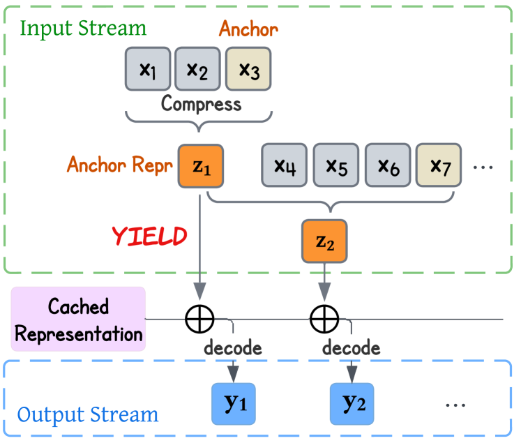
Figure 1: Visualization of our approach. When yield is triggered, the current segment’s information is compressed into an anchor representation to generate the next output.

Locating these triggers poses a significant challenge. Prior approaches have explored methods that employ fixed sliding windows to determine triggers (Ma et al., 2019, 2020b), or learning models to predict triggers (Ma et al., 2020c; Chang & Lee, 2022), yet timing remains a complex issue. Beyond reducing latency, another challenge for stream transduction is how to efficiently represent historical information while optimizing memory usage. Prior work (Rae et al., 2020; Tay et al., 2022; Bertsch et al., 2023, inter alia) has mostly focused on improving the efficiency of Transformer but does not investigate streaming scenarios. Reducing the memory footprint for stream transduction introduces additional complexity as models must determine when certain information becomes less relevant for future predictions.

In this work, we propose Stream Transduction with Anchor Representations (STAR), to maximize the benefits of stream transduction, optimizing both generation latency and memory footprint. STAR introduces the concept of anchors, which aggregate past information (multiple vector representations) into single-vector anchor representations. Once an anchor is yielded, it triggers the generation process. We present a learning strategy to train STAR end-to-end so that the model learns to dynamically select anchor positions with the following objectives: (1) anchors positions are selected such that each segment contains the right amount of information for generating the next output; (2) anchor representation effectively compress the information of its preceding segment. For example, in Figure 1, the model triggers yield at index 3 (which makes it an anchor position), compressing the information of the chunk $\bm{X}=(x_{1},x_{2},x_{3})$ into anchor representation $z_{1}$ to generate output $y_{1}$.

Our contributions are as follows: (1) we propose STAR that dynamically segments and compresses input streams, trading-off among latency, memory footprint, and performance for stream transduction; (2) we demonstrate the effectiveness of our approach on well-established speech-to-text tasks requiring simultaneous processing of long sequences (streams), outperforming existing methods.

2 Methodology

2.1 Problem Formulation

In sequence-to-sequence transduction, high-dimensional feature $\bm{X}=(\bm{x}_{1},\dots,\bm{x}_{T_{x}})$ is normally first extracted from the raw input sequence. Then the decoder can encode and use such features to generate an output sequence $\bm{Y}=(y_{1},\dots,y_{T_{y}})$. The encoder and decoder can be implemented using various models such as Recurrent Neural Networks (Hochreiter & Schmidhuber, 1997; Chung et al., 2014; Lipton, 2015), Transformers (Vaswani et al., 2017), or State-space Models (Gu et al., 2022; Gu & Dao, 2023), depending on the input and output characteristics. In the context of streaming sequence transduction, where the input (and their corresponding features $\bm{X}$) is partially observed, a causal encoder and decoder are necessary. The causal encoder processes the partially observed feature $\bm{X}_{<\tau}$ ($\tau\leq T_{x}$) to produce their encoding. Suppose first $k$ outputs $y_{k}$ are already generated, the causal decoder sample the next output $y_{k+1}$ with $\mathbb{P}(y_{k+1}|\bm{X}_{<\tau},\bm{Y}_{<k+1};\theta)$, where $\theta$ represents the parameter set.

Our approach to tackling stream transduction is outlined in Algorithm 1. It involves a learnable segmenter that scores the importance of each input feature to decide if enough information has been accumulated in the current buffer of features. When yield is triggered to generate new output, the current buffer $\bm{B}$ is compressed into an anchor representation and subsequently used for generation, along with previously cached anchor vectors $\bm{Z}$.

2.2 Segmentation with Dynamic Compression

In this section, we provide details of different components in Algorithm 1. We first present how anchor representations are obtained through our selection-based compression method and then describe how to learn the segmenter with feedback from the encoder-decoder’s cross-attention.

Algorithm 1 High-level overview of STAR

Input: Input stream $\bm{X}$, threshold $\beta$Output: Output stream $\bm{Y}$Initialize: cached repr. $\bm{Z}\leftarrow\varnothing$; buffer $\bm{B}\leftarrow\varnothing$$y\neq\textsc{eos}$$\alpha\leftarrow 0;\bm{B}\leftarrow\varnothing$clear buffer $\bm{x}\leftarrow\textsc{read}(\bm{X})$readnew inputs append($\bm{B},\bm{x}$) add to buffer $\alpha\leftarrow\alpha+F_{\rm seg}(\bm{x})$$\alpha\geq\beta$yield triggered $\bm{H}=F_{\rm enc}(\bm{B}\mid\bm{Z})$encode segment buffer $\bm{z}=\textsc{compress}(\bm{H})$append($\bm{Z},\bm{z})$embedding for segment $y\leftarrow F_{\rm dec}(\cdot|\bm{Y},\bm{Z})$yield$y$break

Compression with Anchor Representation

In this section, we illustrate how anchor representation is computed. To dynamically compress input features for stream transduction, we need a learnable segmenter to partition the input stream. To focus on the compression method, suppose we have already obtained a properly-trained segmenter that labeled several anchor positions as boundaries of partitions (e.g., index 3 & 7 in Figure 1). Every time an anchor is predicted by the segmenter, the model triggers generation with some buffer $\bm{B}\in\mathbb{R}^{b\times d}$ of b features. Subsequently, we transform such features into a high-dimensional representation $\bm{H}\in\mathbb{R}^{b\times d}$ with a causal encoder. The causality of such an encoder ensures that representations at later positions contain information only from earlier positions. Then, we only select the representation at the anchor position (the last index of the current buffer) $\bm{z}=\bm{H}[b]\in\mathbb{R}^{1\times d}$ to represent the information of the whole buffer $\bm{B}$. Selected representations are also called anchor representations/vectors. For example, in Figure 2, yield is triggered at index $3$; therefore we first transform the features into representations $\bm{H}=F_{\rm enc}(\bm{B}|\bm{Z})$, and select $\bm{H}[3]$ as the anchor vector $\bm{z}$ to decode the next output with cached representation $\bm{Z}$.

Our proposed framework, which caches compressed representations, enhances memory efficiency. With a compression rate $r$, a batch size $b$, and input features of average length $T_{x}$, and hidden dimension $d$, our system compresses the encoder representation from $bdT_{x}$ to $bdT_{x}/r$. Besides memory consumption, note that cross-attention computation (Equation 1) is quadratic w.r.t. encoder representation’s length; thus, our method reduces the cost of its computation by a factor of $r^{2}$. In § 5, we perform analysis to benchmark the actual reduction in memory usage with our method.

Learning segmenter with cross-attention

In this section, we propose a learnable segmenter trained with feedback from the encoder-decoder cross-attention. Following Algorithm 1, a segmenter is used to evaluate (score) input features as they are read into the system. Such scores $\bm{s}=F_{\rm seg}(\bm{X})$ are then used to determine if yield is triggered (i.e., whether to segment streams). Effective segmentation is crucial in streaming sequence transduction to avoid sub-optimal transformation due to premature triggering or increased latency from delayed output.

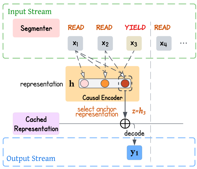
Figure 2: Visualization for the proposed “selection as compression” method. Input features are transformed by the encoder and we only select the encoding at the anchor position (where yield is triggered) as the compressed representation of the block.

Since the ideal segmentation depends on several factors (the input’s information density, the input and output’s modalities, and the task at hand, etc.,), we rely on the cross-attention between the encoder and decoder to guide the segmenter, as shown in Figure 3. Specifically, we follow cross-attention from Transformers (Vaswani et al., 2017) to use three projections $\bm{W}_{\text{Q}},\bm{W}_{\text{K}},\bm{W}_{\text{V}}$ to generate the query vector $\bm{y}\bm{W}_{\text{Q}}\in\mathbb{R}^{T_{y}\times d}$, the key vector $\bm{h}\bm{W}_{\text{K}}\in\mathbb{R}^{T_{x}\times d}$ and the value vector $\bm{h}\bm{W}_{\text{V}}\in\mathbb{R}^{T_{x}\times d}$ (where $d$ is the dimensionality of the representation):

$$\mathrm{softmax}\left(\displaystyle\frac{S(\bm{h},\bm{y})}{\sqrt{d}}\right)\cdot\bm{h}\bm{W}_{\text{V}}$$ (1)

$$S(\bm{h},\bm{y})=(\bm{h}\bm{W}_{\text{k}})(\bm{y}\bm{W}_{\text{Q}})^{T}$$ (2)

Then, as illustrated in Figure 3, we inject segmenter’s scores into it the cross attention:

$$\tilde{S}(\bm{h},\bm{y})=S(\bm{h},\bm{y})+F_{\rm seg}(\bm{x})$$ (3)

The resulting representation will be used by the decoder to compute the loss function during training. Since the segmenter’s scores are injected in Equation 1, it can be updated with end-to-end back-propagation. As the cross-attention computation signals the importance of each position in the encoder to the decoder, we leverage it to effectively train the segmenter to access the input features.

After training the segmenter, we predict scores $\bm{s}=F_{\rm seg}(\bm{x})$ for input features and use the scores to segment the input sequence. Note that the predicted scores can be used differently based on the task. In the special case where the whole sequence is fully observed (i.e., regular non-streaming tasks), we do not yield output anymore. Instead, we simply select the top $k$ scoring positions as anchors and use their representation for the decoder to generate outputs, as formalized below ($I$ is a set of indices):

$$I =\textsc{SelectTop}_{k}(\bm{s})$$ (4)

$$\bm{H} =F_{\rm enc}(\bm{x})\in\mathbb{R}^{T_{x}\times d}$$ (5)

$$\bm{Z} =\bm{H}[I]\in\mathbb{R}^{k\times d}$$ (6)

The compression rate is then $r=T_{x}/k\in[1,\infty)$ assuming $k\leq T_{x}$. In a more general case where streaming is enabled, the score is commonly accumulated (Inaguma et al., 2020; Ma et al., 2020c) until a certain threshold is reached. We use a threshold $\beta=1$ throughout experiments. Specifically, we first scale $\bm{s}$ to $[0,1]$ range values $\bm{\alpha}=\text{sigmoid}(\bm{s})$ and accumulate $\alpha$ following Algorithm 1 (line 8 and 9) to yield new output.

Figure 3: Visualization for the training of the segmenter through feedback from the encoder-decoder’s cross-attention.

2.3 Model Training

To train models for streaming sequence transduction, we primarily rely on the conventional objective – negative log-likelihood (NLL) loss:

$$\mathcal{L}_{\text{NLL}}(\bm{X},\bm{Y},\theta) =-\log\mathbb{P}(\bm{Y}|\bm{X};\theta)$$ (7)

$$=-\sum_{t=1}^{T_{y}}\log\mathbb{P}(y_{t}|\bm{Y}_{<t},\bm{Z}_{<t};\theta),$$ (8)

Note that the loss is defined over $\bm{X},\bm{Y}$ as both input and output sequences are fully observed during training. In addition, the loss defined in Equation 8 is slightly different than regular NLL in that the decoder can only use representation observed so far ($\bm{Z}_{<t}$) to generate the $t^{\text{th}}$ output. This method is also referred to as Infinite-Lookback (Arivazhagan et al., 2019a; Liu et al., 2021, IL) and is used to mitigate the train-test mismatch as future representation cannot be observed during inference.

Besides using NLL to update the encoder and decoder, we have to regularize the segmenter so that the number of yield is the same as the output length $T_{y}$. A common strategy (Chang & Lee, 2022; Dong et al., 2022, inter alia) is to re-scale the scores so that the threshold $\beta$ is reached $T_{y}$ times:

$$\alpha_{t} =\sigma(s_{t})$$ (9)

$$\tilde{\alpha}_{t} =\frac{\beta n^{*}}{\hat{n}}\alpha_{t}=\frac{\beta\cdot T_{y}}{\sum_{t=1}^{T_{x}}\alpha_{t}}\alpha_{t}$$ (10)

Here $\sigma$ is the sigmoid function and $\hat{n}$ is the normalization term (summation of un-scaled scores) and $n^{*}$ denotes the number of desired selections, i.e., $n^{*}=T_{y}$. We assume the input feature is longer than the output ($T_{x}>T_{y}$), so re-scaling scores to yield $T_{y}$ means we employ a dynamic compression rate $r=T_{x}/T_{y}$ while transducing the streams. Note that $T_{y}$ is only observed during training and we cannot re-scale $\bm{s}$ in test time. Therefore, we adopt a length penalty loss (Chang & Lee, 2022; Dong et al., 2022, inter alia) during training to regularize the segmenter to ensure proper learning of segmentations:

$$\mathcal{L}_{\text{lp}}(\bm{X},\bm{Y};\theta) =(n^{*}-\hat{n})^{2}$$

$$=\left(T_{y}-\sum_{t=1}^{T_{x}}\sigma\left(F_{\rm seg}(\bm{x}_{t})\right)\right)^{2}$$ (11)

Finally, our training objective is the combination of negative log-likelihood and length penalty loss:

$$\mathcal{L}(\bm{X},\bm{Y};\theta)=\mathcal{L}_{\text{NLL}}(\bm{X},\bm{Y};\theta)+\gamma\mathcal{L}_{\text{lp}}(\bm{X},\bm{Y};\theta)$$ (12)

In practice, the segmenter is only trained for a few thousand steps (so is the length penalty loss) and we set $\gamma=0.01$. For more details, please refer to appendix D.

3 Experiments: Non-Streaming Compression

We experiment on the non-streaming ASR task to better demonstrate the effectiveness of our selection-based compression method, as we do not need to consider the quality-latency trade-off as in the streaming scenario. We compare our method with other common baselines like Convolutional Neural Networks (Lecun & Bengio, 1995; Krizhevsky et al., 2012, CNN) and Continuous Integrate and Fire (Dong & Xu, 2020, CIF).

Datasets and Evaluation Metrics We conduct experiments on the LibriTTS (Zen et al., 2019) dataset’s “Clean-360h” section, which contains 360 hours of speech and their corresponding transcriptions. To evaluate ASR performance, we compute the word error rate (Morris et al., 2004, WER) between reference transcriptions and the generated text.

3.1 Training Setup

Compression with Anchor Representations

In § 2, we propose a general approach for streaming seq2seq transduction with dynamic compression. Now we instantiate the framework for the ASR task. For details of hyperparamters, we direct readers to Appendix D.

• Feature Extractor: we use Wav2Vec2.0 (Baevski et al., 2020) to extract features from the input speech sequence.

• Encoder: we use a 4-layer decoder-only Transformer.

• Decoder: we also use a 4-layer decoder-only Transformer, with an additional linear layer (language modeling head) to output a distribution over the vocabulary.

• Segmenter: we use a 2-layer feed-forward network.

We freeze the feature extractor (as we used the pre-trained Wav2Vec2.0 model), and train the encoder and decoder from scratch until convergence. This gives a vanilla ASR model for transforming speech input into text, but it does not compress speech representations. To support compression, we follow § 2 to train the segmenter with cross-attention feedback from the pre-trained encoder and decoder. Given the extracted feature $\bm{X}=(x_{1},x_{2},\cdots,x_{T_{x}})$ and a target compression rate $r\in[1,\infty)$, we select top $k=T_{x}/r$ scoring positions and use their encodings as anchor representations (following Equation 6). We then feed the anchor representation $\bm{Z}$ to the decoder to generate text tokens.

In practice, most input speeches from LibriTTS are less than 10 seconds, corresponding to a feature sequence of length $T_{x}=10*16000/320=500$ (with a standard sampling rate 16 kHz and Wav2Vec2.0 has a stack of CNNs that reduce input sequence by 320$\times$). Therefore, we chose some reasonable compression rates (i.e., $r=12,18,30$) to test our compression methods. We briefly describe two baselines that we compared against: CNNs and CIF.

Baseline: CNN A simple compression component is CNN. After we obtain speech feature $\bm{X}$, we apply CNNs with pre-defined strides to compress the feature, then feed the compressed feature into the encoder and decode it with a text decoder. To enhance the capacity of CNNs, we follow Zeghidour et al. (2021); Défossez et al. (2022) to add two CNNs with kernel size $(5,1)$ and stride size $(1,1)$ as residual connection. More details about CNNs and their configurations are available in Figure 14 (in Appendix D).

Baseline: CIF

Continuous Integrate and Fire (CIF, Dong & Xu (2020); Dong et al. (2022); Chang & Lee (2022)) uses a neural network to predict scores for each position and accumulates the scores until a threshold is reached, thereafter triggering the generation of a new token (called fire by the original paper). For each segment, CIF averages representations in the segment by directly weighing them with the predicted scores. For non-streaming ASR, we train the segmenter to fire $k=T_{x}/r$ times, following the re-scale method described in Equation 10.

There are two major differences between our method and CIF: firstly, STAR segmenter leverages cross-attention between encoder-decoder to interactively update representations, whereas CIF employs a weighted average of representations solely from the encoder side; secondly, STAR pushes information to condense in particular anchor at yield positions and performs explicit selections, whereas CIF’s representations are averaged across each segment. Broadly, these distinctions mirror the differences between hard and soft attention mechanisms (Xu et al., 2015; Luong et al., 2015). We refer readers to Appendix B and the original paper (Dong & Xu, 2020) for more details.

3.2 Results of Different Compression Methods

We test the compression performance on three compression rates $r\in\{12,18,30\}$. As shown in Figure 4, our compression module obtains the best performance, achieving almost lossless compression when $r=12$, and consistently outperforms the other two methods on different compression rates. By comparing the trend in detail, we find that CNNs are sub-optimal as the compressor because they operate on a small local window and change the underlying feature representation, which might be hard for the encoder and decoder to adapt to. Now comparing CIF and STAR. As the compression rate increases, the gap between STAR and CIF also increases. When $r=30$, STAR outperforms CIF by about 3 points in WER. From the results, we have verified that STAR is more effective in compressing representation compared to CNN and CIF.

Additionally, in our analysis (see § 5), we provide evidence of STAR achieving more robust compressed representations. Lastly, to exclude the influence from the text decoder, we also designed a speech similarity task in appendix C to show that STAR results in better speech representation.

4 Streaming Experiments: Simultaneous Speech Recognition and Translation

Datasets

For our simultaneous S2T experiments, we use LibriTTS (same as § 3) for ASR. Additionally, we use the English-German (EN-DE) portion of the MuST-C V1 (Di Gangi et al., 2019) dataset for speech translation (ST).

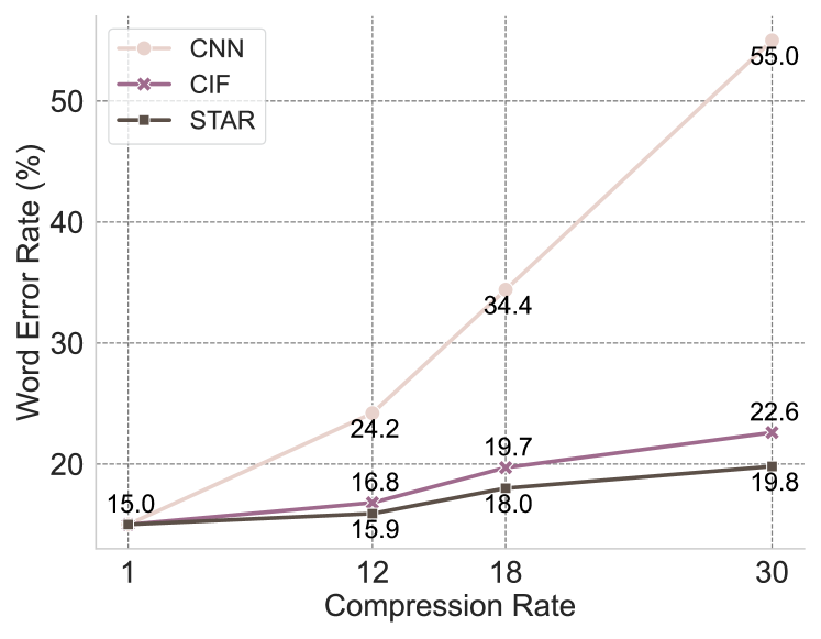
Figure 4: ASR performance (evaluated by WER) by different compression methods. From the figure, STAR outperforms other compressors and the gap enlarges as the compression rate increases.

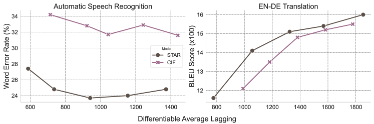
Figure 5: Lateny-Quality trade-off for CIF and STAR. The five markers on the line correspond to different wait-$k$ strategies (from left to right, wait-$k$ $\in\{1,2,3,4,5\}$). Numbers for the plots can be found in Table 8 and Table 8.

Evaluation Metric To evaluate the quality of generated output, we use WER for the ASR task and BLEU (Papineni et al., 2002) for the speech translation task. For simultaneous S2T, latency measurement is essential and we resort to the commonly used metric, Differentiable Average Lagging (Arivazhagan et al., 2019a, DAL), which was originally proposed for simultaneous text translation and later adapted to speech translation in (Ma et al., 2020a). The smaller the DAL, the better the system in terms of latency. Due to space limit, we defer readers to appendix E for details on the latency metric.

Experiment Setup Our first step is to train an speech-to-text (S2T) streaming model without compression. Note that the feature extractor Wav2Vec2.0 is non-causal and does not support streaming input features. Therefore, we add a causal mask to Wav2Vec2.0 and train it jointly with the encoder and decoder until convergence. Once the vanilla streaming S2T model is trained, we freeze the trained causal Wav2Vec2.0 model as the feature extractor and start fine-tuning the encoder and the decoder with the segmenter.

We follow § 2 to re-scale the segmenter’s predicted scores and use the length penalty loss to regularize the segmenter. Then we follow Equation 12 to combine the negative log-likelihood and length penalty loss as the final training objective. Note that, evidently, we did not find Infinite-Lookback (used to regularize NLL loss) beneficial for the quality-latency trade-off in simultaneous EN-DE translation so we only apply IL to simultaneous ASR. This could happen because translation is more complex (since speech and text are no longer monotonically aligned like ASR) and regularization from IL degrades the model’s capability.

During inference, we follow algorithm 1 to generate text tokens. Though CIF and STAR use the same approach to yield new tokens, we emphasize that their segmenters are trained differently and their encoded representations are compressed differently.

Experimental Results

We show the experiment results in Figure 5 where we plot WER/BLEU v.s. DAL to demonstrate the quality-latency trade-off for each system. In our evaluation, we adapt the wait-$k$ policy (Ma et al., 2019) for all systems. Here wait-$k$ denotes the number of speech segments we encode first before decoding text tokens. A larger wait-$k$ value generally results in higher latency but better S2T performance. In our work, we focus on low-latency scenarios as it is where flexible decision policies like CIF and STAR are most useful; thus, we set wait-$k$ value to 1 to 5, corresponding to each marker in Figure 5. Note that if the speech is fully consumed and the text decoder hasn’t reached the eos token, we keep generating text until eos or the maximum number of tokens is reached. If the text decoder predicts the eos token before speech is fully consumed, we stop the decoding process.

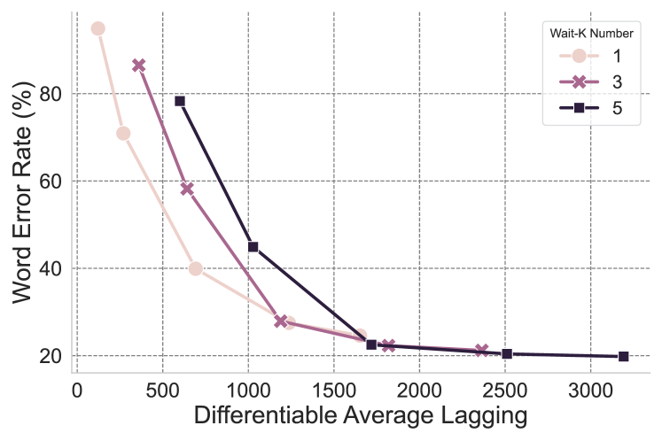
Figure 6: Word Error Rate and Differentiable Average Lagging trade-off for the vanilla S2T model. Each line corresponds to a different wait-$k$ strategy, as shown in the legend. It employs a fixed-decision policy and each marker on the line plot corresponds to a stride size of $\{120,200,280,360,440\}$ms. Numbers for the plots can be found in Table 5.

We first present the baseline system for simultaneous ASR with a fixed decision policy in Figure 6. We use the vanilla streaming S2T model (no compression) and apply a fixed stride size to slide through the speech and generate text tokens. As shown in Figure 6, using a large stride like 360ms (i.e., each chunk corresponds to a speech feature of length $0.36\times 16000/320=18$) or 440ms, simultaneous ASR achieved $<20$ WER. However, the latency is also extremely high. For smaller strides, the quality of generated output is suboptimal because not enough information is provided for the text decoder to generate each new token.

A flexible decision policy could alleviate such issues and provide better latency-quality trade-offs. From Figure 5, we see that for both CIF and STAR, their output has better quality when the latency is low. For instance, STAR achieves about 24 WER with a DAL smaller than 800 while the best-performing fixed decision policy only obtains such performance with a DAL of about 1200.

Comparing CIF with STAR, we find that STAR consistently achieves better performance, obtaining a lower WER (or higher BLEU) score with relatively lower latency across different wait-$k$ strategies. This demonstrates that STAR gives a better flexible policy to yield new tokens, and the compressed representation encodes more information for target text generation. In appendix A, we also compare qualitative examples and visualize the difference in the segmentation from CIF and STAR. Overall, we find the segmentation from STAR better corresponds to the target texts, achieving superior simultaneous S2T performance.

5 Analysis

In this section, we perform additional analysis experiments to showcase STAR’s efficiency and robustness.

Memory Efficiency Recall we calculated earlier that STAR reduces memory usage by $bdT_{x}/r$ for a compression rate $r$, a batch size $b$, and input features of average length $T_{x}$. But what does this mean in real-world application? In this section, we benchmark the actual memory usage and the percentage of usage reduction achieved by different compression rates. From Figure 7, we show that with a rate of $r=10$ (which achieves nearly lossless compression as showed in § 3), STAR reduces the memory consumption by more than 30% when transducing an input feature of length longer than 3,000. For the full details of our benchmark setup and results, we refer readers to Appendix F.

Various Compression Rates at Inference

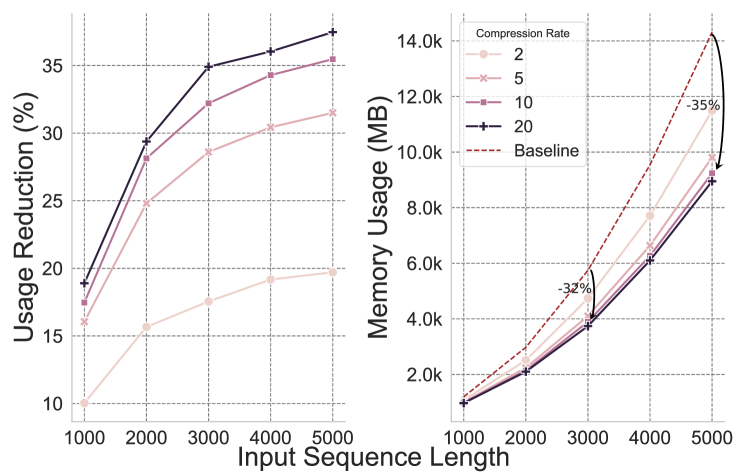
Figure 7: Memory usage and reduction from our proposed method (with compression rates $r\in\{2,5,10,20\}$). More results and detailed setup are provided in appendix F.

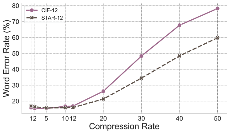
Figure 8: CIF and STAR based model trained with compression rate 12 are evaluated on various compression rates (ranges from 1 to 50). For a lower compression rate ($\leq 12$), both models preserve their quality well. For a higher compression rate ($>12$), STAR is more robust and its performance degrades slower than CIF.

.

In § 3, we trained and evaluated CIF- and STAR-  based model with the same compression rates. In this section, we use the model trained with $r=12$ (denoted as CIF-12 or STAR-12) and test the model on compression rates different from its training scheme. As shown in Figure 8, both STAR-12 and CIF-12 perform well when the compression rate is small (i.e., $r\leq 12$). This is expected because the model is trained to compress by 12$\times$ and is now allowed to have more information. On the other hand, when $r>12$, we find that STAR-12 has a much smaller degradation compared to CIF-12, indicating that STAR’s compressed representation retains more information. STAR’s resilience to higher compression is attributed to forcing the encoder to concentrate information into anchor positions. Consequently, even at high compression rates where fewer anchor representations are selected, each anchor still contains substantial information. In contrast, averaging across positions at high compression rates (CIF) can lead to increased interference between vectors of different positions.

Different Segmentations

In § 4, we train CIF and STAR based models to dynamically compress representation and trigger yield action. Now we try to force both models to use the same fixed decision policy which enforces the same segmentation (i.e., yield at the same time). We segment the speech based on its length and number of target tokens. Now each input chunk has a size $\lfloor T_{x}/T_{y}\rfloor$, which is the average length of speech if it is equally split among the text tokens. The purpose of this analysis is to test if the condensed representation is robust to decision policy (segmentation) changes. As shown in Figure 9, CIF fails when the decision policy is changed; while STAR also suffers performance degradation, it reserves legitimate performance (achieved $<30$ WER with a DAL of 800, while CIF has $>80$ WER). This shows that compressing blocks of information into an anchor representation (STAR) is more robust compared to CIF.

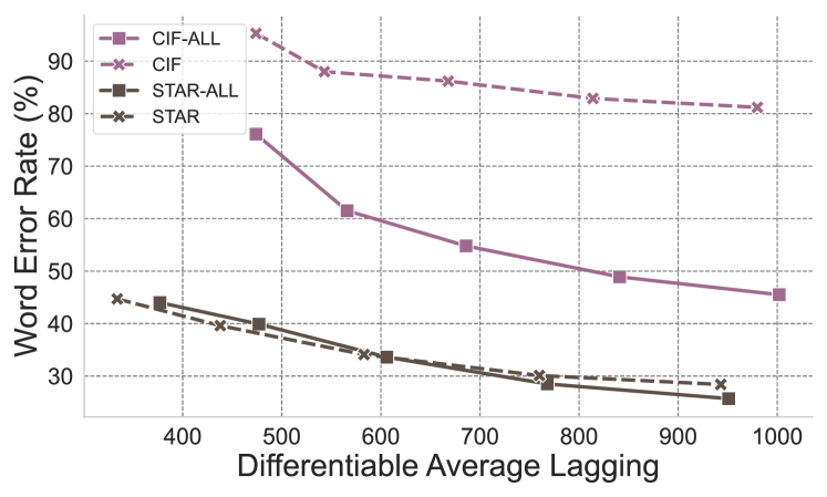
Figure 9: Latency-quality trade-off for CIF and STAR using a fixed decision policy instead of their own predicted segmentation. The five markers on the line correspond to five wait-$k$ strategies (from left to right, wait-$k$ $\in\{1,2,3,4,5\}$). CIF-ALL and STAR-ALL use all embeddings observed so far for each yield. CIF and STAR only use one compressed representation per segment.

Table 1: Word Error Rate of models given the noise injection ratio from 0% to 50%. Best numbers are bolded and better results are highlighted by the blue boxes while bad results are highlighted in yellow boxes . Compared to other compression methods, our proposed STAR is the most robust model across all noise injection ratios. When the noise ratio reaches beyond 30%, STAR even outperforms the S2T model without compression. All compression models are trained with the compression rate 12.

Model	Noise Ratio
	0%	5%	10%	15%	20%	25%	30%	35%	40%	45%	50%
Vanilla S2T	15.0	18.7	23.6	29.6	34.0	38.3	43.7	46.8	51.8	56.1	61.0
S2T + CNN	24.2	26.7	31.9	37.1	40.8	45.5	49.9	53.6	58.9	61.6	65.3
S2T + CIF	16.8	20.4	26.0	30.7	36.0	40.1	44.9	50.1	53.9	58.9	62.2
S2T + STAR	15.9	19.7	25.1	29.8	34.7	38.6	41.8	46.7	51.0	55.6	60.1

Moreover, we let the the two models use all previously computed representations (thus no compression is performed) and name such models ”*-ALL” (see CIF-ALL and STAR-ALL in Figure 9). We find that CIF-ALL still greatly lags behind the performance of STAR even when all previous representations are used. This shows that CIF is not a robust method as it only obtains good performance when aggregating representations using its learned segmentation. On the contrary, STAR is much more robust; in fact, from Figure 9, we find that STAR has a very close performance compared to its non-compressed version STAR-ALL, demonstrating another evidence that STAR  can compress all information into a few positions.

Noise Injection

Lastly, we test the robustness of compression methods when noise is injected into the original clean speech from LibriTTS. Instead of using synthetic signals such as Gaussian noise, we follow Zeghidour et al. (2021) to use natural noise (e.g., noise from the air conditioner, shutting door, etc.,) from Freesound (Fonseca et al., 2017). We vary the ratio of noise injection from 5% to 30%, as shown in Table 1. Given a ratio, we first calculate the duration of noise $L$ (e.g., if the ratio is 0.1 and speech is 10 seconds, then we inject $L=1$ second of noise) and randomly select a range of length $L$ from the clean speech to inject noise. As shown in Table 1, as the noise ratio increases, STAR has the smallest degradation and consistently outperforms CIF and CNNs. After reaching noise ratio $\geq 30\%$, STAR even outperforms the vanilla S2T model without compression. Such findings show that STAR has a more robust performance with the help of anchor representation, making it suffer less from noise injection and obtain better ASR performance.

6 Related Work

Efficient Methods for Transformers Prior work studied efficient methods to scale Transformers to long sequences (Tay et al., 2022), including sparse patterns (Beltagy et al., 2020), recurrence (Dai et al., 2019), kernelized attentions (Choromanski et al., 2021), etc. Some of them can be applied in the streaming settings, such as Streaming LLMs (Xiao et al., 2023), Compressive Transformers (Rae et al., 2020), etc. More recently, Tworkowski et al. (2023); Bertsch et al. (2023) proposed to apply $k$NN to the attention to select a subset of past tokens, akin to the segmentation process in this paper. Similar to the residual connection in our paper, Nugget (Qin & Van Durme, 2023) trains a scorer to select a subset of tokens to represent texts.

Speech Representation Traditionally, acoustic features are extracted by filter-bank features, mel-frequency cepstral coefficients, or bottleneck features (Muda et al., 2010; Davis & Mermelstein, 1980). More recent work relies on self-supervision to learn speech representations. For example, Zeghidour et al. (2021); Défossez et al. (2022) learn acoustic representation by reconstructing the original audio. Latent representation trained from such approaches mostly encodes acoustic information but lacks semantic information (Borsos et al., 2023). To learn semantic representation, masked language modeling, and contrastive learning objectives are popularized by widely used representations from Hubert (Hsu et al., 2021), w2v-BERT (Chung et al., 2021) and Wav2Vec (Schneider et al., 2019; Baevski et al., 2020). All these models use CNNs as a building block to downsample speech signals/representations.

End-to-End Simultaneous Speech Translation For Simultaneous S2T tasks, learning speech representation and policy for read and yield is crucial. Ma et al. (2019) proposed the Wait-K strategy with a fixed decision policy that read chunks of equal-length text for decoding and Ma et al. (2020b) adapts the wait-k strategy for SimulST. Instead of a fixed decision policy, SimulSpeech (Ren et al., 2020) train segmenters with Connectionist Temporal Classification (Graves et al., 2006, CTC) loss. Zeng et al. (2021) also uses CTC for guidance on word boundary learns to shrink the representation and proposes the Wait-K-Stride-N strategy that writes N tokens for each read action. Dong et al. (2022) and Chang & Lee (2022) use CIF to learn segmentation for the speech sequences and trigger the yield action whenever CIF fire a new representation. Additionally, Arivazhagan et al. (2019b); Ma et al. (2020c) supports a more adaptive strategy where dynamic read and yield are possible. However, even for such an adaptive strategy, a good decision policy still matters (Ma et al., 2020b).

7 Conclusion and Future Work

We propose STAR, a model capable of dynamically compressing and transducing streams. STAR consists of a segmenter that is learned through encoder-decoder cross-attention and a selection-based compression method. We verify the effectiveness of STAR through experiments on various speech-to-text tasks. In the future, we hope to extend the framework for streaming non-autoregressive generation.

Supplementary Material

Appendix Sections	Contents
Appendix A	Qualitative Examples of Speech Segmentation
Appendix B	More Details on Continuous Integrate and Fire
Appendix C	Similarity Test for Compressed Speech Representation
Appendix D	Model Configurations and Hyper-parameters
Appendix E	Measuring Latency: Differentiable Average Lagging
Appendix F	Benchmark Memory Usage with/without Compression
Appendix G	Experiments Results Table

Appendix A Qualitative Examples of Speech Segmentation from Compressors

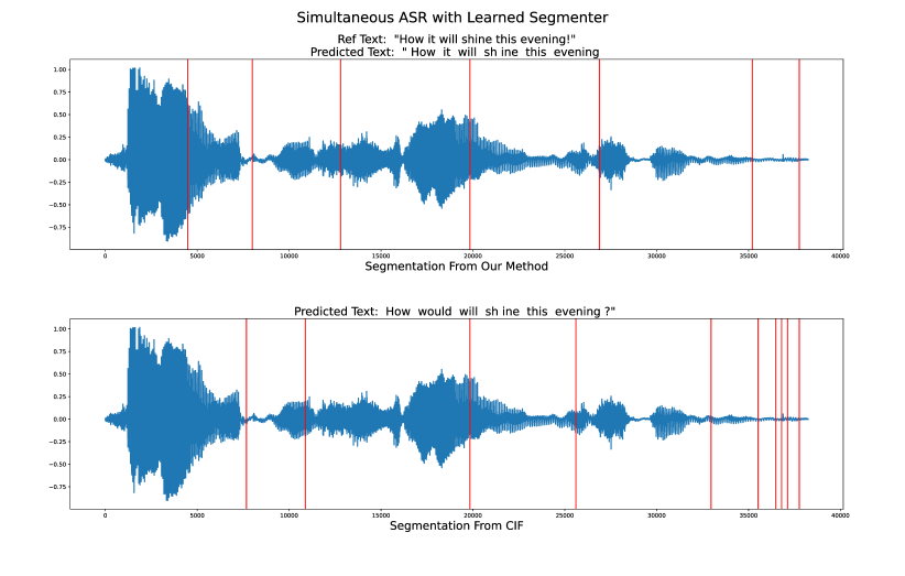
Figure 10: Qualitative Example of CIF and STAR based Segmentation for Simul ASR

.

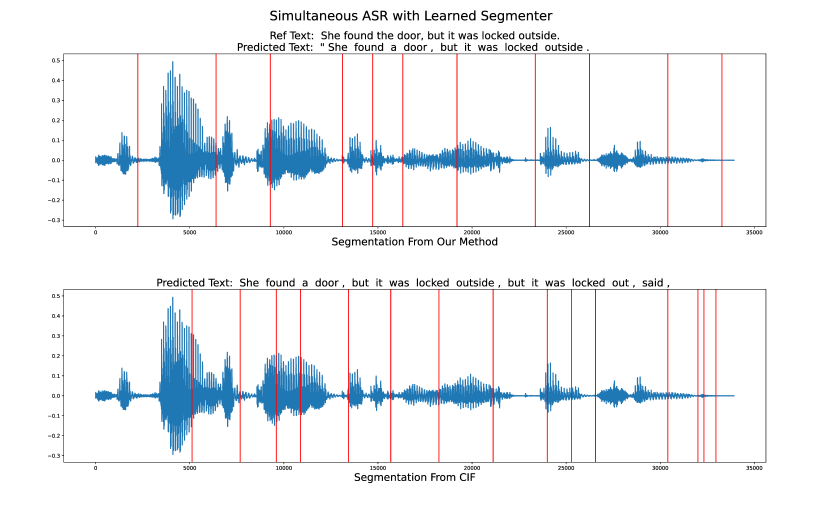
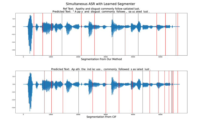
Figure 11: Additional Qualitative Examples of CIF and STAR based Segmentation for Simul ASR

.

Appendix B Continuous Integrate and Fire

Figure 12: Illustration of Continuous Integrate and Fire.

Continuous Integrate and Fire (Dong & Xu, 2020, CIF) predicts a score for each position and dynamically aggregates the semantic representation. As shown in Figure 12, CIF first computes a list of scores $\bm{\alpha}$ similar to our proposed method. Then, starting from the first position, it accumulates the scores (and representation) until reaching a pre-defined threshold $\beta$. Once reaching the threshold, it fire the accumulated representation and starts to accumulate again. As shown in Figure 12, suppose we originally have representation $\bm{z}=(z_{1},\cdots,z_{6})$ with corresponding scores $\bm{\alpha}=(\alpha_{1},\cdots,\alpha_{6})$. Suppose we reach the threshold at $t=3$, $i.e.,\alpha_{1}+\alpha_{2}+\alpha_{3}>=\beta$, then we fire the representation by taking the weighted average of score and representation $c_{1}=\alpha_{1}*\bm{z}_{1}+\alpha_{2}*\bm{z}_{2}+\alpha_{3L}*\bm{z}_{3}$. Here $c_{1}$ becomes the compressed representation for the region $t=[1,3]$. Note that since $\alpha_{1}+\alpha_{2}+\alpha_{3}>=\beta$, we have residual score $\alpha_{3R}=\alpha_{1}+\alpha_{2}+\alpha_{3}-\beta$, which is left for future accumulation, and we only use $\alpha_{3L}=\alpha_{3}-\alpha_{3R}$ when weighting representation $\bm{z}_{3}$. More generally, suppose the previous fire occurs at position $j$ and at current step $i$ the accumulated score reaches the threshold, the aggregated representation is computed as

$$h=\alpha_{jR}*\bm{z}_{j}+\sum_{t=j+1}^{i-1}\alpha_{t}*\bm{z}_{t}+\alpha_{iL}*\bm{z}_{i}$$ (13)

To enforce the compression rate $r$, we follow Dong et al. (2022); Chang & Lee (2022) to re-scale the predicted scores into $s_{t}^{\prime}$ (equation 10). After re-scale the scores, we can ensure that each sequence of representation $\bm{z}\in\mathbb{R}^{l\times d}$ is compressed into $\bm{c}\in\mathbb{R}^{l/r\times d}$.

Our method is fundamentally different because of how we treat the scorer and how we perform compression. In CIF, the compression is performed as an aggregation (weighted average) within each segmented block (decided by the scores and threshold). In STAR, we directly take out representations and we force the semantic encoder to condense information to those important positions. In other words, we did not explicitly perform aggregation like CIF but expect the semantic encoder to learn such aggregation innately through training.

Another key difference is how the scorer is learned. In CIF, the weighted average with scores and representation allows a gradient to flow through the scorer. For STAR, we inject the scores into cross-attention to update the scorer. The major advantage of our approach is that the importance of position is judged by the attention from the decoder to the encoder representation, which helps segment the speech representation in the way that the text decoder perceives it.

For more details, we direct readers to the prior work (Dong & Xu, 2020; Dong et al., 2022; Chang & Lee, 2022).

Appendix C Similarity Test with Compressed Representation

In § 3.2, we show STAR’s superior performance on ASR, demonstrating the effectiveness of condensing information to a few positions for the text decoder. In this section, we evaluate speech representation’s similarity to further probe the quality of the compressed representation, without being influenced by the decoder. More specifically, we use the test set of LibriTTS and for each English transcription, we compute its cosine similarity score against all other transcriptions, using a pre-trained sentence-transformer encoder (it computes a sentence-level representation from BERT and perform mean pooling to obtain a uni-vector representation). We regard the ranking from sentence-Transformer’s similarity as ground truth (as the transcriptions are non-complex English sentences); then we use our speech semantic encoders to compute cosine similarity for all pairs of speech representations and verify if the ranking is similar to the ground truth.

For the baseline vanilla S2T model, we perform mean pooling (MP) on its encoder representation $\bm{c}$ to obtain a uni-vector representation for each speech input and compute cosine similarities. For the other three models with compression, we first obtain the compressed representation $\bm{h}$ and we try two approaches to compute similarity. The first approach is the same as the baseline, where we apply MP on the compressed representation to obtain uni-vector representations. The second approach is inspired by the MaxSim (MS) algorithm used in ColBERT (Khattab & Zaharia, 2020). As illustrated in Figure 13, it computes the average of maximum similarity across the compressed representations.

Then we measure the quality of our trained speech semantic encoders with metrics widely used in retrieval and ranking–Normalized Discounted Cumulative Gain (nDCG) and Mean Reciprocal Rank (MRR). From the results shown in Table 2, STAR still obtains the best-performing representation, with $\text{MRR}@10=0.087,\text{nDCG}@10=0.453$. Note that the performance is not very high as we did not train the model specifically for the sentence similarity task. Rather, we used the similarity task as an intrinsic measurement for the quality of condensed representations to exclude the influence of the text decoder.

Comparing the numbers in Table 2, STAR consistently obtains better speech representation (for both MP and MS algorithms) for the similarity task. Interestingly we find that STAR-30’s representation works better in mean pooling compared to STAR-12, suggesting that more condensed information works better for mean pooling. However, the MaxSim algorithm better leverages the multi-vector representation, which enables STAR-12 to obtain the best ranking performance.

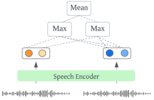
Figure 13: MaxSim algorithm (Khattab & Zaharia, 2020). For each source representation, it computes the maximum similarity by inner producing with all target representations. Then the average of all these maximum similarities is used as the final similarity score

Table 2: Performance of speech rankings by different representation. STAR achieves the best performance as evaluated by NDCG@10 and MRR@10. The best performance is achieved through the MaxSim algorithm; interestingly, STAR-30 achieves the best performance with the Mean Pooling algorithm.

	NDCG @ 10		MRR @ 10
Model	MP	MS	MP	MS
Vanilla S2T	0.407	N/A	0.053	N/A
Conv-12	0.399	0.41	0.035	0.053
CIF-12	0.418	0.444	0.056	0.078
STAR-12	0.429	0.453	0.064	0.087
STAR-18	0.429	0.446	0.055	0.078
STAR-30	0.437	0.441	0.078	0.08

Appendix D Hyper-parameters

We provide hyper-parameters used for model configuration and training in this section. For different compression rates, the CNNs’ stride configuration is shown in Figure 14. For example, a stride of (4,3) means we stack two CNN blocks, one with stride 4 and another with stride 3, achieving a compression rate of 12.

In this section, we provide the hyper-parameters and training configurations for all our experiments. We use a hidden dimension of 512 across all models. The tokenizer is developed using Byte Pair Encoding (Sennrich et al., 2016, BPE), with a vocabulary size of 10,000. The segmenter is parameterized by a 2-layer FFN with ReLU (Agarap, 2018) activation in between; the first FFN has input and output dimensions both set to 512 and the second FFN has input dimension 512 with output dimension 1. Our experiments are conducted using the Adam optimizer, configured with $\beta_{1}=0.9$ and $\beta_{2}=0.999$. These experiments are conducted with a data-parallel setting with 4 A100 GPUs.

For the audio processing, we set the sampling rate to 16,000. In the encoder configuration, we use a maximum of 1,024 positions for Automatic Speech Recognition (ASR) and 2,048 for Speech Translation (ST), with each encoder consisting of 4 layers and 8 attention heads. The decoder mirrors the encoder in its architecture, with 4 layers and 8 attention heads, but differs in its maximum positions, set at 512, and its vocabulary size, also at 10,000.

For non-streaming ASR in our pre-training setup, both the encoder and decoder are trained to converge with a learning rate of 1e-4, a batch size of 32, and a warmup of 10,000 steps. Subsequently, the compression module (CNN/CIF/STAR) is fine-tuned using a learning rate of 5e-5 alongside the pre-trained encoder and decoder. The segmenter is trained for 6,000 steps with feedback from the encoder-decoder’s cross-attention, as discussed in Section § 2, after which it is frozen. Post this, we further fine-tune the encoder and decoder until convergence.

For streaming speech-to-text tasks, the feature extractor (Wav2Vec2.0), encoder, and decoder are jointly trained with a learning rate of 5e-5, a batch size of 8, and gradient accumulation every 4 steps. A causal mask is added to Wav2Vec2.0during this process. Following convergence, the compression module undergoes fine-tuning using a learning rate of 5e-5 and a batch size of 16. Similar to the non-streaming setup, the segmenter is updated only in the first 6,000 steps.

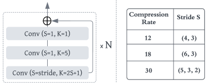
Figure 14: Left: Blocks of CNNs used to compress representation. Right: Stride sizes we used in experiments for different compression rates.

Appendix E Differentiable Average Lagging

Consider a raw speech with length $T_{x}$ which is segmented into $|X|$ chunks. We define the length of $i^{th}$ segment (chunk) as $|X_{i}|$ (so that $|X|=\sum_{j=1}^{|X|}|X_{j}|$), and we define $d_{i}=\sum_{t=1}^{i}|X_{t}|$ as the total time that has elapsed until $i^{th}$ speech segment $X_{i}$ is processed. With the aforementioned notation, DAL is defined to be:

$$\text{DAL}=\frac{1}{T_{y}}\sum_{i=1}^{T_{y}}d_{i}^{\prime}-\frac{i-1}{\gamma}$$ (14)

where $T_{y}$ is the length of text tokens and $1/\gamma$ is the minimum delay after each operation, computed as $1/\gamma=\sum_{j=1}^{|X|}|X_{j}|/T_{y}$ (i.e., the averaged elapsed time for each token is used as the minimum delay). Lastly, $d_{i}^{\prime}$ is defined as:

$$d_{i}^{\prime}=\begin{cases}d_{i}&i=0\\ \text{max}(d_{i},d_{i-1}^{\prime}+1/\gamma)&i>0\end{cases}$$ (15)

The smaller the DAL, the better the system in terms of latency. For more discussions for DAL and latency-quality trade-off in SimulST, we direct readers to prior work (Ma et al., 2020a; Arivazhagan et al., 2019a) for more details.

Appendix F Memory Usage Benchmark

In this section, we describe our setup to benchmark memory usage, which compares our proposed approach with a vanilla encoder-decoder model that does not support compression. We use Google Colab with a runtime that uses a T4 (16G memory) GPU. Then for each experiment, we run it 5 times and report the average in Table 3. Both encoder and decoders follow our setup in appendix D, except that encoder’s maximum position is increased to 8,196 to support the benchmark experiment with long sequences. Note that the sequence length reported is the length of the input feature (which we compress by $r\in\{2,5,10,20\}$). We set the output sequence’s length to be $\frac{1}{10}$ of the input, similar to the ratio in our simultaneous speech-to-text experiments.

Table 3: Memory usage (MB) of the encoder-decoder model with and without our proposed compression method. OOM: out of memory.

Stage	Batch Size	Seq Len	No Compression	With Compression
				r=2	r=5	r=10	r=20
Inference	1	1000	1196	1076	1004	987	970
	1	2000	2975	2509	2237	2138	2101
	1	3000	5744	4736	4101	3894	3739
	1	4000	9540	7711	6637	6269	6102
	1	5000	14314	11493	9805	9237	8951
	1	6000	OOM	OOM	13587	12786	12434
Training	128	100	4964	4730	4209	4160	4124
	128	200	10687	9948	9465	9302	9223

Appendix G Experiments Results Tables

Table 4: Model Performance with various compression rates. The performance is evaluated by Word Error Rate and BLEU score. The number is presented as WER (BLEU). STAR achieves the best performance across three compression methods, and is almost lossless when the compression rate is 12.

Model	Compression Rate
	1	12	18	30
Conv	15 (77.6)	24.2 (65.5)	34.4 (57.4)	55 (40.2)
CIF	15 (77.6)	16.8 (74.9)	19.7 (70.3)	23 (67.1)
STAR	15 (77.6)	15.9 (75.2)	18 (73)	20 (70.4)

Table 5: Quality-latency trade-off of the streaming S2T model without compression, tested on simultaneous ASR task using the LibriTTS dataset. It uses a fixed decision policy, based on varying wait-k and stride sizes shown above.

Wait-K	Stride Size	DAL	WER
1	120ms	122	94.9
	200ms	270	70.9
	280ms	692	39.9
	360ms	1236	27.5
	440ms	1652	24.6
3	120ms	360	86.5
	200ms	642	58.2
	280ms	1189	27.9
	360ms	1819	22.3
	440ms	2364	21.2
5	120ms	600	78.3
	200ms	1028	44.9
	280ms	1719	22.5
	360ms	2511	20.4
	440ms	3192	19.8

Table 6: Quality-latency trade-off of the streaming S2T model with compression modules, tested on LibriTTS and Must-C’s English-German datasets. Both CIF and STAR use a flexible decision policy based on their scorer predictions. We experiment with different wait-k numbers using models’ flexible decision policies.

Table 7: Latency-Quality trade-off for Simultaneous ASR

	STAR		CIF
Wait-K	DAL	WER	DAL	WER
1	588	27.4	714	34.2
2	736	24.8	923	32.8
3	941	23.7	1044	31.7
4	1155	24.0	1243	32.9
5	1373	24.8	1440	31.6

Table 8: Latency-Quality trade-off for Simultaneous English-German Translation

	STAR		CIF
Wait-K	DAL	BLEU	DAL	BLEU
1	777	11.6	990	12.1
2	1056	14.1	1181	13.5
3	1325	15.1	1381	14.8
4	1568	15.4	1581	15.2
5	1853	16.0	1778	15.5

References

- Agarap (2018) Agarap, A. F. Deep learning using rectified linear units (relu). ArXiv, abs/1803.08375, 2018. URL https://api.semanticscholar.org/CorpusID:4090379.
- Arivazhagan et al. (2019a) Arivazhagan, N., Cherry, C., Macherey, W., Chiu, C.-C., Yavuz, S., Pang, R., Li, W., and Raffel, C. Monotonic infinite lookback attention for simultaneous machine translation. pp. 1313–1323, 01 2019a. doi: 10.18653/v1/P19-1126.
- Arivazhagan et al. (2019b) Arivazhagan, N., Cherry, C., Macherey, W., Chiu, C.-C., Yavuz, S., Pang, R., Li, W., and Raffel, C. Monotonic infinite lookback attention for simultaneous machine translation. In Korhonen, A., Traum, D., and Màrquez, L. (eds.), Proceedings of the 57th Annual Meeting of the Association for Computational Linguistics, pp. 1313–1323, Florence, Italy, July 2019b. Association for Computational Linguistics. doi: 10.18653/v1/P19-1126. URL https://aclanthology.org/P19-1126.
- Baevski et al. (2020) Baevski, A., Zhou, H., Mohamed, A., and Auli, M. wav2vec 2.0: A framework for self-supervised learning of speech representations, 2020.
- Barrault et al. (2023) Barrault, L., Chung, Y.-A., Meglioli, M. C., Dale, D., Dong, N., Duppenthaler, M., Duquenne, P.-A., Ellis, B., Elsahar, H., Haaheim, J., Hoffman, J., Hwang, M.-J., Inaguma, H., Klaiber, C., Kulikov, I., Li, P., Licht, D., Maillard, J., Mavlyutov, R., Rakotoarison, A., Sadagopan, K. R., Ramakrishnan, A., Tran, T., Wenzek, G., Yang, Y., Ye, E., Evtimov, I., Fernandez, P., Gao, C., Hansanti, P., Kalbassi, E., Kallet, A., Kozhevnikov, A., Gonzalez, G. M., Roman, R. S., Touret, C., Wong, C., Wood, C., Yu, B., Andrews, P., Balioglu, C., Chen, P.-J., Costa-jussà, M. R., Elbayad, M., Gong, H., Guzmán, F., Heffernan, K., Jain, S., Kao, J., Lee, A., Ma, X., Mourachko, A., Peloquin, B., Pino, J., Popuri, S., Ropers, C., Saleem, S., Schwenk, H., Sun, A., Tomasello, P., Wang, C., Wang, J., Wang, S., and Williamson, M. Seamless: Multilingual expressive and streaming speech translation, 2023.
- Beltagy et al. (2020) Beltagy, I., Peters, M. E., and Cohan, A. Longformer: The Long-Document Transformer, 2020. URL http://arxiv.org/abs/2004.05150.
- Bertsch et al. (2023) Bertsch, A., Alon, U., Neubig, G., and Gormley, M. R. Unlimiformer: Long-Range Transformers with Unlimited Length Input, 2023. URL http://arxiv.org/abs/2305.01625.
- Borsos et al. (2023) Borsos, Z., Marinier, R., Vincent, D., Kharitonov, E., Pietquin, O., Sharifi, M., Roblek, D., Teboul, O., Grangier, D., Tagliasacchi, M., and Zeghidour, N. Audiolm: a language modeling approach to audio generation, 2023.
- Chang & Lee (2022) Chang, C.-C. and Lee, H.-y. Exploring continuous integrate-and-fire for adaptive simultaneous speech translation. In Interspeech 2022. ISCA, September 2022. doi: 10.21437/interspeech.2022-10627. URL http://dx.doi.org/10.21437/Interspeech.2022-10627.
- Chen et al. (2021) Chen, J., Ma, M., Zheng, R., and Huang, L. Direct simultaneous speech-to-text translation assisted by synchronized streaming asr. In Findings, 2021. URL https://api.semanticscholar.org/CorpusID:235422036.
- Choromanski et al. (2021) Choromanski, K., Likhosherstov, V., Dohan, D., Song, X., Gane, A., Sarlos, T., Hawkins, P., Davis, J., Mohiuddin, A., Kaiser, L., Belanger, D., Colwell, L., and Weller, A. Rethinking Attention with Performers. In International Conference on Learning Representations (ICLR), 2021. URL http://arxiv.org/abs/2009.14794.
- Chung et al. (2014) Chung, J., Gulcehre, C., Cho, K., and Bengio, Y. Empirical evaluation of gated recurrent neural networks on sequence modeling, 2014.
- Chung et al. (2021) Chung, Y.-A., Zhang, Y., Han, W., Chiu, C.-C., Qin, J., Pang, R., and Wu, Y. W2v-bert: Combining contrastive learning and masked language modeling for self-supervised speech pre-training, 2021.
- Dai et al. (2019) Dai, Z., Yang, Z., Yang, Y., Carbonell, J., Le, Q. V., and Salakhutdinov, R. Transformer-XL: Attentive Language Models Beyond a Fixed-Length Context. In Annual Meeting of the Association for Computational Linguistics (ACL), 2019. URL http://arxiv.org/abs/1901.02860.
- Davis & Mermelstein (1980) Davis, S. and Mermelstein, P. Comparison of parametric representations for monosyllabic word recognition in continuously spoken sentences. IEEE Transactions on Acoustics, Speech, and Signal Processing, 28(4):357–366, 1980. doi: 10.1109/TASSP.1980.1163420.
- Devlin et al. (2019) Devlin, J., Chang, M.-W., Lee, K., and Toutanova, K. Bert: Pre-training of deep bidirectional transformers for language understanding. In North American Chapter of the Association for Computational Linguistics, 2019. URL https://api.semanticscholar.org/CorpusID:52967399.
- Di Gangi et al. (2019) Di Gangi, M. A., Cattoni, R., Bentivogli, L., Negri, M., and Turchi, M. MuST-C: a Multilingual Speech Translation Corpus. In Burstein, J., Doran, C., and Solorio, T. (eds.), Proceedings of the 2019 Conference of the North American Chapter of the Association for Computational Linguistics: Human Language Technologies, Volume 1 (Long and Short Papers), pp. 2012–2017, Minneapolis, Minnesota, June 2019. Association for Computational Linguistics. doi: 10.18653/v1/N19-1202. URL https://aclanthology.org/N19-1202.
- Dong & Xu (2020) Dong, L. and Xu, B. Cif: Continuous integrate-and-fire for end-to-end speech recognition, 2020.
- Dong et al. (2022) Dong, Q., Zhu, Y., Wang, M., and Li, L. Learning when to translate for streaming speech. In Muresan, S., Nakov, P., and Villavicencio, A. (eds.), Proceedings of the 60th Annual Meeting of the Association for Computational Linguistics (Volume 1: Long Papers), pp. 680–694, Dublin, Ireland, May 2022. Association for Computational Linguistics. doi: 10.18653/v1/2022.acl-long.50. URL https://aclanthology.org/2022.acl-long.50.
- Défossez et al. (2022) Défossez, A., Copet, J., Synnaeve, G., and Adi, Y. High fidelity neural audio compression, 2022.
- Fonseca et al. (2017) Fonseca, E., Pons, J., Favory, X., Font, F., Bogdanov, D., Ferraro, A., Oramas, S., Porter, A., and Serra, X. Freesound datasets: A platform for the creation of open audio datasets. 10 2017.
- Graves et al. (2006) Graves, A., Fernández, S., Gomez, F., and Schmidhuber, J. Connectionist temporal classification: Labelling unsegmented sequence data with recurrent neural networks. In Proceedings of the 23rd International Conference on Machine Learning, ICML ’06, pp. 369–376, New York, NY, USA, 2006. Association for Computing Machinery. ISBN 1595933832. doi: 10.1145/1143844.1143891. URL https://doi.org/10.1145/1143844.1143891.
- Gu & Dao (2023) Gu, A. and Dao, T. Mamba: Linear-time sequence modeling with selective state spaces, 2023.
- Gu et al. (2022) Gu, A., Goel, K., and Ré, C. Efficiently modeling long sequences with structured state spaces. In The International Conference on Learning Representations (ICLR), 2022.
- Gulati et al. (2020) Gulati, A., Qin, J., Chiu, C., Parmar, N., Zhang, Y., Yu, J., Han, W., Wang, S., Zhang, Z., Wu, Y., and Pang, R. Conformer: Convolution-augmented transformer for speech recognition. CoRR, abs/2005.08100, 2020. URL https://arxiv.org/abs/2005.08100.
- Hochreiter & Schmidhuber (1997) Hochreiter, S. and Schmidhuber, J. Long short-term memory. Neural Computation, 9(8):1735–1780, 1997.
- Hsu et al. (2021) Hsu, W.-N., Bolte, B., Tsai, Y.-H. H., Lakhotia, K., Salakhutdinov, R., and Mohamed, A. Hubert: Self-supervised speech representation learning by masked prediction of hidden units, 2021.
- Inaguma et al. (2020) Inaguma, H., Gaur, Y., Lu, L., Li, J., and Gong, Y. Minimum latency training strategies for streaming sequence-to-sequence asr. ICASSP 2020 - 2020 IEEE International Conference on Acoustics, Speech and Signal Processing (ICASSP), pp. 6064–6068, 2020. URL https://api.semanticscholar.org/CorpusID:215737044.
- Kameoka et al. (2021) Kameoka, H., Tanaka, K., and Kaneko, T. Fasts2s-vc: Streaming non-autoregressive sequence-to-sequence voice conversion. ArXiv, abs/2104.06900, 2021. URL https://api.semanticscholar.org/CorpusID:233231613.
- Khattab & Zaharia (2020) Khattab, O. and Zaharia, M. A. Colbert: Efficient and effective passage search via contextualized late interaction over bert. Proceedings of the 43rd International ACM SIGIR Conference on Research and Development in Information Retrieval, 2020. URL https://api.semanticscholar.org/CorpusID:216553223.
- Krizhevsky et al. (2012) Krizhevsky, A., Sutskever, I., and Hinton, G. E. Imagenet classification with deep convolutional neural networks. In Pereira, F., Burges, C., Bottou, L., and Weinberger, K. (eds.), Advances in Neural Information Processing Systems, volume 25. Curran Associates, Inc., 2012. URL https://proceedings.neurips.cc/paper_files/paper/2012/file/c399862d3b9d6b76c8436e924a68c45b-Paper.pdf.
- Lecun & Bengio (1995) Lecun, Y. and Bengio, Y. Convolutional Networks for Images, Speech and Time Series, pp. 255–258. The MIT Press, 1995.
- Li (2021) Li, J. Recent advances in end-to-end automatic speech recognition. ArXiv, abs/2111.01690, 2021. URL https://api.semanticscholar.org/CorpusID:240419899.
- Li et al. (2020) Li, X., Wang, C., Tang, Y., Tran, C., Tang, Y., Pino, J. M., Baevski, A., Conneau, A., and Auli, M. Multilingual speech translation from efficient finetuning of pretrained models. In Annual Meeting of the Association for Computational Linguistics, 2020. URL https://api.semanticscholar.org/CorpusID:227840539.
- Lipton (2015) Lipton, Z. C. A critical review of recurrent neural networks for sequence learning. CoRR, abs/1506.00019, 2015. URL http://arxiv.org/abs/1506.00019.
- Liu et al. (2021) Liu, D., Du, M., Li, X., Li, Y., and Chen, E. Cross attention augmented transducer networks for simultaneous translation. In Moens, M.-F., Huang, X., Specia, L., and Yih, S. W.-t. (eds.), Proceedings of the 2021 Conference on Empirical Methods in Natural Language Processing, pp. 39–55, Online and Punta Cana, Dominican Republic, November 2021. Association for Computational Linguistics. doi: 10.18653/v1/2021.emnlp-main.4. URL https://aclanthology.org/2021.emnlp-main.4.
- Liu et al. (2019) Liu, Y., Xiong, H., He, Z., Zhang, J., Wu, H., Wang, H., and Zong, C. End-to-end speech translation with knowledge distillation. In Interspeech, 2019. URL https://api.semanticscholar.org/CorpusID:119309065.
- Luong et al. (2015) Luong, T., Pham, H., and Manning, C. D. Effective approaches to attention-based neural machine translation. In Màrquez, L., Callison-Burch, C., and Su, J. (eds.), Proceedings of the 2015 Conference on Empirical Methods in Natural Language Processing, pp. 1412–1421, Lisbon, Portugal, September 2015. Association for Computational Linguistics. doi: 10.18653/v1/D15-1166. URL https://aclanthology.org/D15-1166.
- Ma et al. (2019) Ma, M., Huang, L., Xiong, H., Zheng, R., Liu, K., Zheng, B., Zhang, C., He, Z., Liu, H., Li, X., Wu, H., and Wang, H. STACL: Simultaneous translation with implicit anticipation and controllable latency using prefix-to-prefix framework. In Korhonen, A., Traum, D., and Màrquez, L. (eds.), Proceedings of the 57th Annual Meeting of the Association for Computational Linguistics, pp. 3025–3036, Florence, Italy, July 2019. Association for Computational Linguistics. doi: 10.18653/v1/P19-1289. URL https://aclanthology.org/P19-1289.
- Ma et al. (2020a) Ma, X., Dousti, M. J., Wang, C., Gu, J., and Pino, J. SIMULEVAL: An evaluation toolkit for simultaneous translation. In Liu, Q. and Schlangen, D. (eds.), Proceedings of the 2020 Conference on Empirical Methods in Natural Language Processing: System Demonstrations, pp. 144–150, Online, October 2020a. Association for Computational Linguistics. doi: 10.18653/v1/2020.emnlp-demos.19. URL https://aclanthology.org/2020.emnlp-demos.19.
- Ma et al. (2020b) Ma, X., Pino, J., and Koehn, P. SimulMT to SimulST: Adapting simultaneous text translation to end-to-end simultaneous speech translation. In Wong, K.-F., Knight, K., and Wu, H. (eds.), Proceedings of the 1st Conference of the Asia-Pacific Chapter of the Association for Computational Linguistics and the 10th International Joint Conference on Natural Language Processing, pp. 582–587, Suzhou, China, December 2020b. Association for Computational Linguistics. URL https://aclanthology.org/2020.aacl-main.58.
- Ma et al. (2020c) Ma, X., Pino, J. M., Cross, J., Puzon, L., and Gu, J. Monotonic multihead attention. In International Conference on Learning Representations, 2020c. URL https://openreview.net/forum?id=Hyg96gBKPS.
- Morris et al. (2004) Morris, A. C., Maier, V., and Green, P. D. From wer and ril to mer and wil: improved evaluation measures for connected speech recognition. In Interspeech, 2004. URL https://api.semanticscholar.org/CorpusID:18880375.
- Muda et al. (2010) Muda, L., Begam, M., and Elamvazuthi, I. Voice recognition algorithms using mel frequency cepstral coefficient (mfcc) and dynamic time warping (dtw) techniques, 2010.
- Papineni et al. (2002) Papineni, K., Roukos, S., Ward, T., and Zhu, W.-J. Bleu: a method for automatic evaluation of machine translation. In Isabelle, P., Charniak, E., and Lin, D. (eds.), Proceedings of the 40th Annual Meeting of the Association for Computational Linguistics, pp. 311–318, Philadelphia, Pennsylvania, USA, July 2002. Association for Computational Linguistics. doi: 10.3115/1073083.1073135. URL https://aclanthology.org/P02-1040.
- Qin & Van Durme (2023) Qin, G. and Van Durme, B. Nugget: Neural agglomerative embeddings of text. In Krause, A., Brunskill, E., Cho, K., Engelhardt, B., Sabato, S., and Scarlett, J. (eds.), Proceedings of the 40th International Conference on Machine Learning, volume 202 of Proceedings of Machine Learning Research, pp. 28337–28350. PMLR, 23–29 Jul 2023. URL https://proceedings.mlr.press/v202/qin23a.html.
- Rae et al. (2020) Rae, J. W., Potapenko, A., Jayakumar, S. M., and Lillicrap, T. P. Compressive Transformers for Long-Range Sequence Modelling. In International Conference on Learning Representations (ICLR), 2020. URL http://arxiv.org/abs/1911.05507.
- Ren et al. (2020) Ren, Y., Liu, J., Tan, X., Zhang, C., Qin, T., Zhao, Z., and Liu, T.-Y. SimulSpeech: End-to-end simultaneous speech to text translation. In Jurafsky, D., Chai, J., Schluter, N., and Tetreault, J. (eds.), Proceedings of the 58th Annual Meeting of the Association for Computational Linguistics, pp. 3787–3796, Online, July 2020. Association for Computational Linguistics. doi: 10.18653/v1/2020.acl-main.350. URL https://aclanthology.org/2020.acl-main.350.
- Schneider et al. (2019) Schneider, S., Baevski, A., Collobert, R., and Auli, M. wav2vec: Unsupervised pre-training for speech recognition, 2019.
- Sennrich et al. (2016) Sennrich, R., Haddow, B., and Birch, A. Neural machine translation of rare words with subword units. In Erk, K. and Smith, N. A. (eds.), Proceedings of the 54th Annual Meeting of the Association for Computational Linguistics (Volume 1: Long Papers), pp. 1715–1725, Berlin, Germany, August 2016. Association for Computational Linguistics. doi: 10.18653/v1/P16-1162. URL https://aclanthology.org/P16-1162.
- Somogyi (2021) Somogyi, Z. Automatic speech recognition. The Application of Artificial Intelligence, 2021. URL https://api.semanticscholar.org/CorpusID:4660196.
- Tay et al. (2022) Tay, Y., Dehghani, M., Bahri, D., and Metzler, D. Efficient Transformers: A Survey. ACM Computing Surveys, 55(6):1–28, 2022. URL http://arxiv.org/abs/2009.06732.
- Tworkowski et al. (2023) Tworkowski, S., Staniszewski, K., Pacek, M., Wu, Y., Michalewski, H., and Miłoś, P. Focused Transformer: Contrastive Training for Context Scaling, 2023. URL http://arxiv.org/abs/2307.03170.
- Vaswani et al. (2017) Vaswani, A., Shazeer, N., Parmar, N., Uszkoreit, J., Jones, L., Gomez, A. N., Kaiser, L. u., and Polosukhin, I. Attention is all you need. In Guyon, I., Luxburg, U. V., Bengio, S., Wallach, H., Fergus, R., Vishwanathan, S., and Garnett, R. (eds.), Advances in Neural Information Processing Systems, volume 30. Curran Associates, Inc., 2017. URL https://proceedings.neurips.cc/paper_files/paper/2017/file/3f5ee243547dee91fbd053c1c4a845aa-Paper.pdf.
- Wang et al. (2022) Wang, P., Sun, E., Xue, J., Wu, Y., Zhou, L., Gaur, Y., Liu, S., and Li, J. Lamassu: A streaming language-agnostic multilingual speech recognition and translation model using neural transducers. INTERSPEECH 2023, 2022. URL https://api.semanticscholar.org/CorpusID:258968116.
- Xiao et al. (2023) Xiao, G., Tian, Y., Chen, B., Han, S., and Lewis, M. Efficient Streaming Language Models with Attention Sinks, 2023. URL http://arxiv.org/abs/2309.17453.
- Xu et al. (2015) Xu, K., Ba, J., Kiros, R., Cho, K., Courville, A., Salakhudinov, R., Zemel, R., and Bengio, Y. Show, attend and tell: Neural image caption generation with visual attention. In Bach, F. and Blei, D. (eds.), Proceedings of the 32nd International Conference on Machine Learning, volume 37 of Proceedings of Machine Learning Research, pp. 2048–2057, Lille, France, 07–09 Jul 2015. PMLR. URL https://proceedings.mlr.press/v37/xuc15.html.
- Xue et al. (2022) Xue, J., Wang, P., Li, J., Post, M., and Gaur, Y. Large-scale streaming end-to-end speech translation with neural transducers. In Interspeech, 2022. URL https://api.semanticscholar.org/CorpusID:248118691.
- Zeghidour et al. (2021) Zeghidour, N., Luebs, A., Omran, A., Skoglund, J., and Tagliasacchi, M. Soundstream: An end-to-end neural audio codec, 2021.
- Zen et al. (2019) Zen, H., Dang, V., Clark, R., Zhang, Y., Weiss, R. J., Jia, Y., Chen, Z., and Wu, Y. Libritts: A corpus derived from librispeech for text-to-speech, 2019.
- Zeng et al. (2021) Zeng, X., Li, L., and Liu, Q. RealTranS: End-to-end simultaneous speech translation with convolutional weighted-shrinking transformer. In Zong, C., Xia, F., Li, W., and Navigli, R. (eds.), Findings of the Association for Computational Linguistics: ACL-IJCNLP 2021, pp. 2461–2474, Online, August 2021. Association for Computational Linguistics. doi: 10.18653/v1/2021.findings-acl.218. URL https://aclanthology.org/2021.findings-acl.218.